Online Optimization in XOnline Optimization in X--

Armed BanditsArmed BanditsCS101.2

January 20th, 2009

Paper by S. Bubeck, R. Munos, G. Stoltz, C. Szepersvári

Slides by C. Chang

Review of BanditsReview of Bandits

� Started with k arms

◦ Integral, finite domain of arms

◦ General idea: Keep track of average and confidence for each arm

◦ Expected regret using UCB1 = O(log n)

Review of BanditsReview of Bandits

� Last week

� Bandit arms against “adversaries”

◦ Oblivious

� O(n2/3)

◦ Adaptive

� O(n3/4)

Extending the ArmsExtending the Arms

� What about infinitely many arms?

� Draw arms from X = [0, 1]D

◦ D-dimensional vector of values from 0 to 1

� Mean-payoff function, f, maps from X�

R

� No adversaries (fixed payoffs)

Extending the ArmsExtending the Arms

� What if there are no restrictions on the shape of f?

Extending the ArmsExtending the Arms

� What if there are no restrictions on the shape of f?

� Then we don’t know anything about arms we haven’t pulled

Extending the ArmsExtending the Arms

� What if there are no restrictions on the shape of f?

� Then we don’t know anything about arms we haven’t pulled

� With infinitely many arms, this means we can’t do anything!

Extending the ArmsExtending the Arms

� Okay, so no continuity at all goes too far

� Generalize the mean-payoff function function to be “pretty smooth”

� That way, we can (hopefully) get information about a neighborhood of arms from a single pull

� We will use Lipschitz continuity

Lipschitz ContinuityLipschitz Continuity

� Intuitively, the slope of the function is bounded

� That is, it never increases or decreases faster than a certain rate

� This seems like it can give us information about an area with a single pull

Lipschitz ContinuityLipschitz Continuity

� Formal definition:

� Function f(x) is Lipschitz continuous if,

� Given a dissimilarity function, d(x,y),

� f(x) – f(y) ≤ k × d(x,y)

� k is the Lipschitz constant

Lipschitz ContinuityLipschitz Continuity

� For a function f with a certain constant k, we call the function k-Lipschitz

� We’ll assume 1-Lipschitz

◦ For another k, we can just adjust the payoffs to make the function 1-Lipschitz

◦We’re really just concerned with relative performance versus other strategies on the same f

Lipschitz ContinuityLipschitz Continuity

Function will stay inside the green cone(Graphic taken with permission from Wikipedia underGNU Free Documentation License 1.2)

Lipschitz FunctionsLipschitz Functions

� Examples of functions that are Lipschitz:

Lipschitz FunctionsLipschitz Functions

� Examples of functions that are Lipschitz:

◦ f(x) = sin(x)

◦ f(x) = |x|

◦ f(x,y) = x + y

Lipschitz FunctionsLipschitz Functions

� Examples of functions that are Lipschitz:

◦ f(x) = sin(x)

◦ f(x) = |x|

◦ f(x,y) = x + y

� And functions that aren’t:

Lipschitz FunctionsLipschitz Functions

� Examples of functions that are Lipschitz:

◦ f(x) = sin(x)

◦ f(x) = |x|

◦ f(x,y) = x + y

� And functions that aren’t:

◦ f(x) = x2

◦ f(x) = x / (x – 3)

ApplicationApplication

� Why would we need a bandit arm strategy for non-linear mean-payoff functions?

ApplicationApplication

� One example: Modeling airflow over a plane wing

� A parameter vector is an arm

� Pulling an arm is costly

◦ Difficult to actually calculate (computer models, PDEs…)

� Still want to maximize some kind of result across the arms

Developing an AlgorithmDeveloping an Algorithm

� Okay, so it’s useful

� What kind of algorithm should we use?

� Random?

◦We’ve seen how well this works out

� Other obvious approaches are less applicable with infinitely many arms…

Developing an AlgorithmDeveloping an Algorithm

� We can reuse the ideas from the UCB1

algorithm

p1 p2 p3p4

Adjustments NeededAdjustments Needed

� Not discrete arms, but a continuum

◦We will have need a UCB for all arms over the arm-space

� We can get some confidence about any pulled arm’s neighbors because of Lipschitz

Stumbling AroundStumbling Around

� Not discrete arms, but a continuum…

[0] x D [1] x D

Stumbling AroundStumbling Around

� New points affect their neighbors

[0] x D [1] x D

Adjustments NeededAdjustments Needed

� We can also sharpen our estimates from nearby measurements

� Retain “optimism in the face of the unknown”

� General idea gotten…but how do we actually do it?

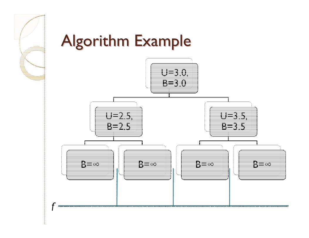
The Algorithm!The Algorithm!

� Split the arm-space into regions

� Every time you pick an arm from a region, divide into more precise regions

� Keep track of how good every region is through results of itself and its children.

Setup for the AlgorithmSetup for the Algorithm

� To remember regions, use a “Tree of Coverings”

� A node in the tree with height h and row-index i is represented as Ph,i or just (h,i)

◦ The children of Ph,i are Ph+1,2i-1 and Ph+1,2i◦ The whole arm-space X = P0,1

� The children of a node cover their parent

Setup for the AlgorithmSetup for the Algorithm

� We always choose a leaf node, then add its children to the tree.

� Each node has a “score” – we pick a new leaf by going down the tree, going to the side with the greater score.

� Score:

Bh,i(n) = min{Uh,i(n), maxchildren[Bchild]}

where Uh,i(n) is the upper confidence bound for the tree node (h,i)

Setup for the AlgorithmSetup for the Algorithm

� One more caveat – For any node (h,i), the diameter (determined by d, the dissimilarity function) of the smallest circle that bounds the node is less than ν1ρ

h for some parameters ν,ρ

� A little more formally,

Uh,i(n) = µh,i(n) + Chernoff + ν1ρh

(Chernoff = sqrt[(2 ln n) / Nh,i(n)] )

Setup for the AlgorithmSetup for the Algorithm

� Score:

Bh,i(n) = min{Uh,i(n), maxchildren[Bchild]}

� What if you have no children?

Setup for the AlgorithmSetup for the Algorithm

� Score:

Bh,i(n) = min{Uh,i(n), maxchildren[Bchild]}

� What if you haven’t been picked yet?

� Optimism in the face of uncertainty!

◦ Set B to infinity

Algorithm ExampleAlgorithm Example

f

Algorithm ExampleAlgorithm Example

f

Algorithm ExampleAlgorithm Example

fY = 0.5

Algorithm ExampleAlgorithm Example

fY = 0.5

Algorithm ExampleAlgorithm Example

f

ObservationsObservations

� Exploration comes from the pessimism of the B-score and the optimism of the unknown

� Exploitation comes from the optimism of the B-score and fast elimination of bad parts of the function

Numerical ResultsNumerical Results

� The following is taken from another talk by the author, Sébastien Bubeck

Numerical ResultsNumerical Results

Regret Analysis Regret Analysis

� Not going to go through all the math◦ If want, read the paper...

� Pretty similar to regret analysis of UCB1

◦ Number of times a bad arm is chosen is proportional to log(n) and inverse to difference to best arm

◦ Add a lot of mess from the Lipschitzness

◦ Actually, we only require “weak-Lipschitz”, which is a sort of one-sided Lipschitz near the best arms

Regret AnalysisRegret Analysis

� Main result:

� E(Rn) ≤ C(d') n(d'+1)/(d'+2)(ln n)1/(d'+2)

◦ C is some constant

◦ d' is any number greater than d, and in most cases, can be equal to d

Regret AnalysisRegret Analysis

� E(Rn) ≤ C(d') n(d'+1)/(d'+2)(ln n)1/(d'+2)

� For high d, we get closer and closer to linear...

◦ "The Curse of Dimensionality"

� This is proven to be tight! Tight!

Dissimilarity FunctionsDissimilarity Functions

� We’ve just been using straight distance

� d can be any metric

◦ d(x,y) = 0 iff x = y

◦ d must be symmetric

◦ Triangle inequality

� With creative dissimilarity functions, this is surprisingly powerful!

Powerful DissimilaritiesPowerful Dissimilarities

� Suppose we go back to the example of online ads

� Ads sell all sorts of products (not quite infinite, but still more than we’d want to try individually!

� Can’t we get information from knowing that some ads are related?

Online Product SalesOnline Product Sales

Online Product SalesOnline Product Sales

� Dissimilarity function should measure how, well, dissimilar two ads are.

� Can take the tree, weight the edges as, say, 1/h, and compute distance

� Can now use the hierarchical algorithm!

� New dissimilarity functions add a lot of mileage...