MRI Brain image segmentation using graph cuts
56
MRI Brain image segmentation using graph cuts Master of Science Thesis in Communication Engineering Mohammad Shajib Khadem Signal Processing Group Department of Signals and Systems CHALMERS UNIVERSITY OF TECHNOLOGY Göteborg, Sweden, 2010 Report No. EX072/2010
Transcript of MRI Brain image segmentation using graph cuts
MRI Brain image segmentation using
graph cuts
Master of Science Thesis in Communication Engineering
Mohammad Shajib Khadem
Signal Processing Group
Department of Signals and Systems
CHALMERS UNIVERSITY OF TECHNOLOGY
Göteborg, Sweden, 2010 Report No. EX072/2010
1
MRI Brain image segmentation using graph cuts
Thesis for the degree of Master of Science
Mohammad Shajib Khadem
Supervisor and Examiner: Professor Irene Yu-Hua Gu
Department of Signals and Systems
Signal Processing Group
CHALMERS UNIVERSITY OF TECHNOLOGY
Göteborg, Sweden, Oct., 2010
2
Abstract
Over the last few years the graph cuts method became very popular in image processing and
analysis area due to smoothness and energy minimization. Brain Magnetic Resonance Image
(MRI) segmentation is a complex problem in the field of medical imaging despite various
presented methods. MR image of human brain can be divided into several sub-regions especially
soft tissues such as gray matter, white matter and cerebrospinal fluid. The graph cuts are used in
medical image segmentation following few dynamic algorithms. The combinatorial optimized
algorithm with the minimum cut and maximum flow techniques provides solution to overcome
the associated challenges of segmented brain MRI. The min-cut/max-flow algorithm comprises
three predominant stages- growth, augmentation and adoption with two non-overlapping search
trees � ��� � and roots at the source � and the sink � respectively. This thesis paper investigates
two algorithms to segment brain tissues and to implement the competent one through simulations
by MATLAB software. Image pre-processing, edges and boundaries detection, histogram
thresholding and segmentation with graph cuts will be performed in applying the selected
method. Segmentation results comparison by the existing software tool of the normalized cut
algorithm and applied simulations of the min-cut/max flow algorithm provide quantitative brain
image analysis. Evaluation of segmented tissues by these methods is based on ground truth
labeling and time consumption and will represent the standard benchmarks for segmentation.
Further research will lead this pixel based automatic segmentation in distinguishing more brain
tissues and performance improvement.
Key words: Magnetic Resonance Imaging (MRI), segmentation, graph cuts, min-cut/max flow,
normalized cut.
3
Contents
Abstract 2
Contents 3
Acknowledgements 5
1. Introduction 6
1.1 Background 6
1.2 Problems and challenges of brain image segmentation 7
1.3 Scopes and objectives of the thesis 7
1.4 Outline 7
2. Brief review of segmentation methods 8
2.1 Mean shift 8
2.2 Histogram thresholding 8
2.3 Region growing 10
2.4 Edge based segmentation 10
2.5 Graph cuts segmentation 11
2.6 Fuzzy connectivity 12
2.7 Optimal single and multiple surface segmentation 13
3. Graph Cuts: Theory 14
3.1 Graph partitioning for image segmentation 14
3.2 Min-cut/max-flow algorithm for graph cuts 18
3.3 Normalized graph cut 19
3.4 Brain image segmentation using a combination of softwares 20
3.4.1 The MRIcroN software 20
3.4.2 FMRIB Software Library (FSL) 20
4. Test systems for brain image segmentation 21
4.1 Pre-processing (block-1) 21
4.2 Segmentation (block-2) 24

4
5. Experimental Results 38
5.1 Brain image segmentation using the normalized cut algorithm 39
5.2 Brain image segmentation using the min-cut/max-flow algorithm 42
6. Discussions and Conclusions 49
6.1 Discussions 49
6.2 Conclusions 49
Appendix 51
Bibliography 53
List of Figures 54
List of Tables 55

5
Acknowledgements
This thesis work wouldn’t have been successfully completed without the constant support of a
number of people and I would like to express my sincere gratitude to them for their spontaneous
help and encouragement.
First of all, I would like to thank my supervisor and examiner Prof. Irene Yu-Hua Gu for
providing me the opportunity to work on the brain MR image segmentation. Throughout the
entire project period her depth of knowledge on the topic, suggestions for continuous
improvement, encouragement and supervision helped me to conduct this research work
productively. Besides, she has been very concerned on the project progress, which has made this
project as a successful one.
I would also like to thank Mr. Fhang and Dr. Imad for assisting me out during the entire project
period with various resources, constructive suggestions and ideas which helped me in a number
of ways.
I am deeply thankful and want to express my honest appreciations to my dear friends Kallol,
Tilak, Johan, Shuvo, Asif, Rupok who helped me time to time with problem solving, idea
generation, and providing required project related information. I appreciate their precious time,
assistance and moral support.
Finally, my heartfelt thanks go to my wife, Rifat Sharmelly, my parents and all my family
members for believing in me and inspiring me during the project duration.
6
1. Introduction
Segmentation subdivides an image into its regions of components or objects and an important
tool in medical image processing [1]. As an initial step segmentation can be used for
visualization and compression. Through identifying all pixels (for two dimensional image) or
voxels (for three dimensional image) belonging to an object, segmentation of that particular
object is achieved [2]. In medical imaging, segmentation is vital for feature extraction, image
measurements and image display [2, 3]. Segmentation of the brain structure from magnetic
resonance imaging (MRI) has received paramount importance as MRI distinguishes itself from
other modalities and MRI can be applied in the volumetric analysis of brain tissues such as
multiple sclerosis, schizophrenia, epilepsy, Parkinson’s disease, Alzheimer’s disease, cerebral
atrophy, etc [4]. Graph cuts is one the image segmentation techniques which is initiated by
interactive or automated identification of one or more points representing the 'object'. In this
technique one or more points representing the 'background' are called seeds and serve as
segmentation hard constraints where as the soft constraints reflect boundary and/or region
information. An important feature of this technique is its ability to interactively improve a
previously obtained segmentation in an efficient way.
1.1 Background
In image segmentation the level to which the subdivision of an image into its constituent regions
or objects is carried depends on the problem being solved. In other words, when the object of
focus is separated, image segmentation should stop [1]. The main goal of segmentation is to
divide an image into parts having strong correlation with areas of interest in the image.
Segmentation can be primarily classified as complete and partial. Complete segmentation results
in a set of disjoint regions corresponding solely with input image objects. While in partial
segmentation resultant regions do not correspond directly with input image [5]. Image
segmentation is often treated as a pattern recognition problem since segmentation requires
classification of pixels [2].
In medical imaging for analyzing anatomical structures such as bones, muscles blood vessels,
tissue types, pathological regions such as cancer, multiple sclerosis lesions and for dividing an
entire image into sub regions such as the white matter (WM), gray matter (GM) and
cerebrospinal fluid (CSF) spaces of the brain automated delineation of different image
components are used [2, 3]. In the field of medical image processing segmentation of MR brain
image is significant as MRI is particularly suitable for brain studies because of its excellent
contrast of soft issues, non invasive characteristic and a high spatial resolution.
Graph-cuts are one of the emerging image segmentation techniques for brain tissue
identification. It has been introduced for image analysis since 2001 through global energy
minimization [6]. It is used with various algorithms for quantitative analysis, content based
image search. The efficient graph cuts algorithm performs optimal and accurate segmentation
with minimum cut and maximum flow.
Image segmentation is an essential tool in medical image processing and is used in various
applications. For example, in medical imaging filed is used to detect multiple sclerosis lesion
7
quantification, surgical planning, conduct surgery simulations, locate tumors and other
pathologies, measure tissue volumes, brain MRI segmentation, study of anatomical structure etc
[3]. Other practical applications of image segmentation are machine vision, traffic control
system, face and finger print recognition and locate objects in satellite images. Image
segmentation with graph cuts technique has potential usefulness for everyday applications like
image cropping and colorization along with the multi-view image stitching, video texture
synthesis, image reconstruction, n-dimensional image segmentation etc [5].
1.2 Problems and challenges of brain image segmentation
There are a number of techniques to segment an image into regions that are homogeneous. Not
all the techniques are suitable for medical image analysis because of complexity and inaccuracy.
There is no standard image segmentation technique that can produce satisfactory results for all
imaging applications like brain MRI, brain cancer diagnosis etc. Optimal selection of features,
tissues, brain and non–brain elements are considered as main obstacles for brain image
segmentation. Accurate segmentation over full field of view is another hindrance. Operator
supervision and manual thresholding are other barriers to segment brain image. During the
segmentation procedure verification of results is another source of difficulty.
1.3 Scopes and objectives of the thesis
Various medical imaging techniques such as magnetic resonance imaging (MRI), computed
tomography (CT) provide different perspectives on the human brain. Many segmentation
techniques such as mean shift, region growing, water shed, graph cuts, fuzzy connectivity etc.
are available for medical imaging especially for brain MRI. Graph-cuts are one of the leading
segmentation techniques to efficiently solve a wide variety of brain tissue identification. Energy
minimization along with image smoothing is performed with the graph cuts method. Different
types of algorithms such as new minimum-cut/maximum flow (min-cut/max-flow), push-relabel,
augmenting paths etc. are used in graph cuts method as well as the normalized cut.
The aim of this thesis is to perform brain MR image segmentation applying the min-cut/max-
flow algorithm of graph cuts technique. In this regard, MATLAB simulations with the mentioned
algorithm will be conducted to implement in graph cuts technique. Results comparison of the
min-cut/max-flow algorithm with the normalized cut will be accomplished to evaluate
segmentation quality.
1.4 Outline
The thesis is organized as follows. Chapter 1 provides the introductory part and background
information of the thesis topic as well as research scopes and goals identification. Literature
review of various segmentation techniques and different kinds of algorithms are discussed in
Chapter 2. Theoretical analysis of graph-cuts technique, problem formulation and
methodological approach of the new minimum cut/maximum flow algorithm is depicted in
Chapter 3 which is the foundation of this thesis work. Simulation results with MATLAB
software applying the algorithm are presented in Chapter 4. Detailed discussions and quantitative
evaluation of the results are explored and analyzed in Chapter 5. Finally conclusions have been
made in Chapter 6 along with recommendations for future research work.

8
2. Brief review of segmentation methods
This chapter provides a brief literature study of the segmentation techniques used in medical
image analysis. Segmentation of an object in an image is performed either by locating all pixels
or voxels that form its boundary or by identifying them that belong to the object. In medical
imaging, segmentation is an important analysis function for which lots of algorithms and
methods have been built up. Variability of data is quite high in medical image processing
especially for analyzing anatomical structure and tissue types [2]; hence segmentation techniques
that provide flexibility, accuracy and convenient automation are of paramount importance.
2.1 Mean shift
Mean shift method is a non-parametric technique to examine a complex multi-modal feature
space and to classify feature clusters. Size and shape of the region of interest are the only free
parameters in this method. In mean shift segmentation in order to estimate the density gradient,
the density estimation is changed. A two step sequence of discontinuity preserving filtering and
mean shift clustering is utilized in this segmentation technique [5]. In mean shift process for each
point in data space first, the region of interest is obtained like a spherical window [hs hr]. Next,
the mean shift is calculated as below.
,� �� � ∑ ��� ��� � ��� �������∑ � ��� � ��� �������
� �
Here, �� is the initial estimate of this iterative method, � ������ �� can be considered as the
kernel function which determines the weight of nearby points for re-estimation of the mean.
Lastly, the center is shifted to the new one unless the mode is found. This algorithm places � ,� ��and repeating is occurred until ,� �� is converged to �.
2.2 Histogram thresholding
The most uncomplicated image segmentation process is histogram thresholding since
thresholding is fast and economical in computation. For segmenting background and objects, a
threshold which is defined as brightness constant is used. Band thresholding, local thresholding,
multi thresholding and semi- thresholding are some of the modifications of this technique. Single
thresholds that can differ in image elements are known as local threshold whereas Single
thresholds that can be applied to the complete image are known as global threshold. In order to
determine the threshold automatically, threshold recognition approaches are exploited. Threshold
recognition approaches can employ optimal thresholding, p-tile thresholding and histogram
shape analysis. Optimal thresholding results in minimum error segmentation as the threshold as
the closest gray-level corresponding to the minimum probability between the maxima of two or
more normal distributions is established through this approach. For color or multi band images
multi-spectral thresholding is suitable. As a minimum between the two highest local maxima, in
bi-modal histograms the threshold is verified [5].

9
In the approach where based on the image histogram only one threshold is chosen for the
complete image, then it is called global thresholding. It is assumed that the object in interest can
be extracted from the background comparing image values having threshold value T (32,132)
and the image has a bimodal histogram. In Figure 1, the bimodal histogram of an image f(x, y)
with selected threshold T has been illustrated.
Figure 1. Bimodal histogram of an image f(x, y) with selected threshold T [2].
The threshold image g(x,y) can be represented as below:
� �, !� � "1 $% �, !� & �0 $% �, !� ( � )
The resultant image is a binary image from global thresholding where pixels that correspond to
objects and background have value 1 and 0 respectively. Simple and rapid calculation is the main
advantages of global thresholding [2]. When thresholding relies on local properties of some
image regions, then it is called local thresholding. It can be established in either of the two ways.
In the first way through dividing an image into sub images and calculating threshold for each sub
image thresholding can be obtained. In the other way image intensities in the region of each pixel
is studied and thresholding is obtained.
Image histogram can be made better through applying image preprocessing techniques. Image
smoothing is one this preprocessing technique. Gaussian filter is one of the smoothing filters
where based on a Gaussian function convolution mask coefficients are g [i, j] for each pixel [i,
j].
�*$, +, � -�.� $� / +��21�
Here σ refers to the spread parameter. Better image smoothing is implied through larger σ.
10
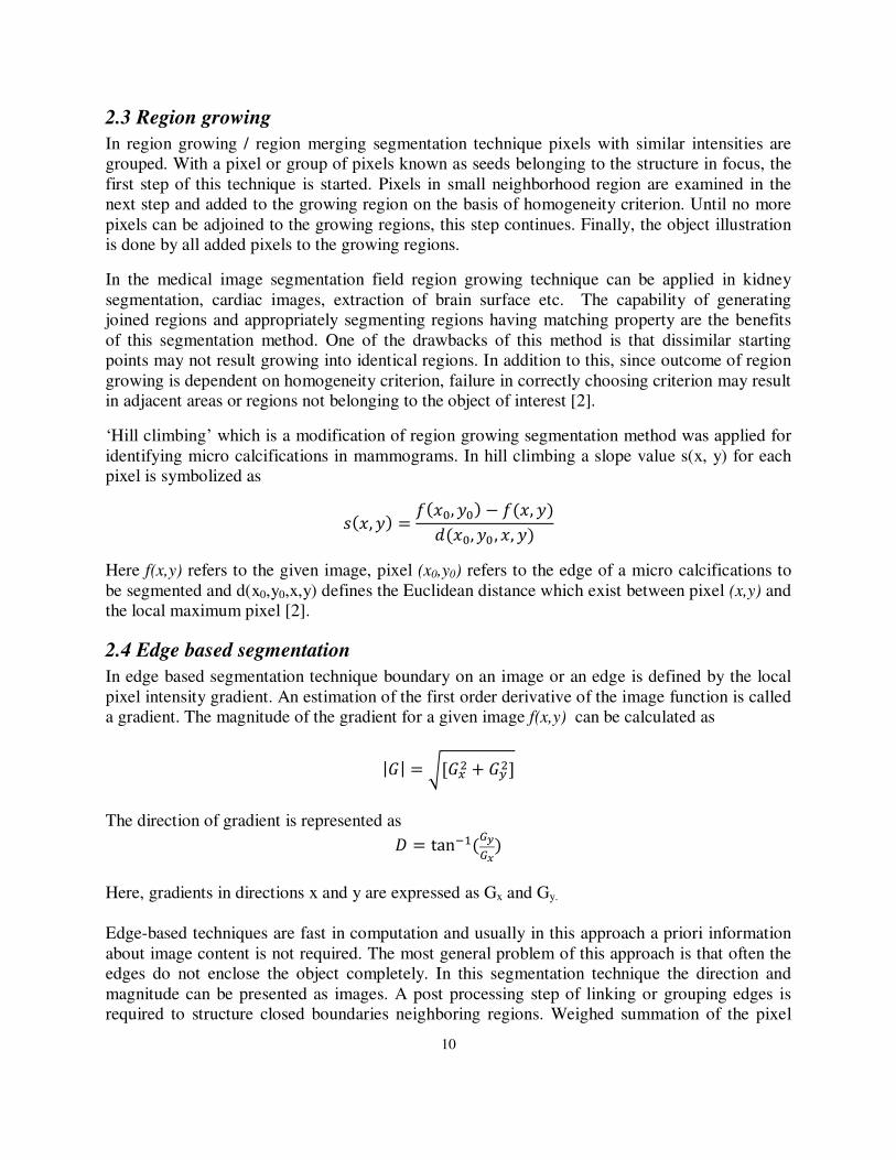
2.3 Region growing
In region growing / region merging segmentation technique pixels with similar intensities are
grouped. With a pixel or group of pixels known as seeds belonging to the structure in focus, the
first step of this technique is started. Pixels in small neighborhood region are examined in the
next step and added to the growing region on the basis of homogeneity criterion. Until no more
pixels can be adjoined to the growing regions, this step continues. Finally, the object illustration
is done by all added pixels to the growing regions.
In the medical image segmentation field region growing technique can be applied in kidney
segmentation, cardiac images, extraction of brain surface etc. The capability of generating
joined regions and appropriately segmenting regions having matching property are the benefits
of this segmentation method. One of the drawbacks of this method is that dissimilar starting
points may not result growing into identical regions. In addition to this, since outcome of region
growing is dependent on homogeneity criterion, failure in correctly choosing criterion may result
in adjacent areas or regions not belonging to the object of interest [2].
‘Hill climbing’ which is a modification of region growing segmentation method was applied for
identifying micro calcifications in mammograms. In hill climbing a slope value s(x, y) for each
pixel is symbolized as
� �, !� � % �2, !2� � % �, !�� �2, !2 , �, !�
Here f(x,y) refers to the given image, pixel (x0,y0) refers to the edge of a micro calcifications to
be segmented and d(x0,y0,x,y) defines the Euclidean distance which exist between pixel (x,y) and
the local maximum pixel [2].
2.4 Edge based segmentation
In edge based segmentation technique boundary on an image or an edge is defined by the local
pixel intensity gradient. An estimation of the first order derivative of the image function is called
a gradient. The magnitude of the gradient for a given image f(x,y) can be calculated as
|4| � 5*4�� / 46�,
The direction of gradient is represented as 7 � tan�� �;�<�
Here, gradients in directions x and y are expressed as Gx and Gy.
Edge-based techniques are fast in computation and usually in this approach a priori information
about image content is not required. The most general problem of this approach is that often the
edges do not enclose the object completely. In this segmentation technique the direction and
magnitude can be presented as images. A post processing step of linking or grouping edges is
required to structure closed boundaries neighboring regions. Weighed summation of the pixel
11
intensities in a small neighborhood can be represented as a numerical array in this method which
is called as kernel/ window/mask. In a two 3X3 mask the following matrices are used.
=�1 �2 �10 0 01 2 1 > =�1 0 1�2 0 2�1 0 1>
To compute Gx and Gy, first and second mask are used respectively. Finally, joining Gx and Gy
using the mentioned equation, gradient magnitude image is obtained [2].
2.5 Graph cuts segmentation
Solving the pixel labeling problem is one of the most frequent applications of energy
minimization in Computer Vision. Through pixel labeling problems image restoration,
segmentation, problems as stereo and motion are generalized. In general energy functions like E
are non convex functions in large dimension spaces and hence very difficult to minimize.
However, when these energy functions have special characteristics, it is possible to find their
exact minimum using dynamic programming. Nonetheless, it is usually necessary to rely on
general minimization techniques, in the general case, like Simulated Annealing [7], which can be
very slow in practice. A property of a graph cut C is that it can be related to a labeling f, mapping
the set of vertices V−{s, t} of a graph G to the set {0, 1}, where f(v) = 0, if v ∈S, and f(v) = 1, if
v ∈ T. A binary partitioning of the vertices of the graph is defined through this labeling.
Graph cut optimization has become well accepted in the area of early vision since it was
proposed as an efficient way to minimize a larger class of energy functions. Various problems as
image segmentation [8], [9], image restoration [10], [11], [12], image synthesis [13], stereo and
motion [10], [11], [14], [15], [16] can be solved by graph cuts. The optimality of graph cut
minimization methods depends on the number of labels and the exact form of the smoothness
term V. In [12] is proved that when the problem is a binary labeling problem, the method yields
global minimum solutions, while in [14] proved that, it is possible to compute global minimal, if
the smoothness term is restricted to a convex function. Creation of a specific graph for every
specific problem was required in the early proposals utilizing graph cut optimization as a
technique for energy minimization. A common scheme for graph cut minimization of energy
functions has been introduced in [17].
Numerous graph techniques are existed which are exploited in image segmentation such as
minimum spanning trees, shortest path, graph-cuts etc. Among all these typical graph
partitioning methods graph-cuts are comparatively new and the most powerful one for image
segmentation [5]. Flexible and accurate global optimization and computation efficiency are
achieved with graph cuts segmentation. Graph-cut segmentation was first initiated as binary
image reconstruction approach in Greig et al. 1969. The graph optimization algorithm such as the
combination of min-cut and max-flow was presented in Boykov and Jolly, 2001 as a powerful
method of optimal boundary and region segmentation in n-D image data. The method was
initiated by them for automated identification of ‘object’ and ‘background’ with the terms seeds,
segmentation hard constraints and soft constraints for region information.
12
Image segmentation relates basically background and object which can be employed as binary
labeling problem. Boykov and Jolly [9] mentioned the segmentation of a monochrome image
that solves a two labels problem in the graph cut method. Considering a set of labels L and a set
of sites S, the labeling problem can be assigned as a label %?@A and each of the site .@�. The
label set A � B0,1C where 0 indicates background and 1 indicates object. For a labeling problem
if % � D%?E%?@AF for all pixels, the energy minimization Markov Random Field (MRF) equation
[5] can be written as:
G %� �H7?I%?J / K H L?M . � %? O %M�B?,MCPQ?PR
In the energy minimization equation, the first term called as data term consists of constraints
from the observed data and measures how the labels are assigned. Label fp fits with site p and is
measured by Dp. The second term which is the smoothness term measures to what extent f is not
piecewise smooth. N represents the neighborhood system like 4 or 8-connected system. If %? � %M , � %? O %M� becomes 0 and 1 otherwise. In image segmentation it is expected the
boundary to be positioned on the edges. Hence the typical selection of ωpq is:
L?M � -� ST�SU�V
�WV . 1�$�� ., X� Color values of Sites p and q are represented by Ip and Iq along with distance between p and q is
presented by dist (p,q). Level of variation between neighboring sites is expressed by the
parameter δ. The relative importance of the data term versus smoothness term is revealed by the
parameter λ.
Most of the existing graph-cuts algorithm can be categorized in two predominant groups viz.
augmenting path method of Ford and Fulkerson , 1969 and push-relabel method of Goldberg and
Tarjan , 1988 [5]. The augmenting path algorithm shows that the flow is pushed through the
graph from source, s to sink, t until the maximum flow is reached. If no flow is present between s
and t, the process is initialized with zero flow status. In the push-relabel algorithm, the excess
flow is pushed towards the nodes with shorter estimated distances to the sink. A labeling of
nodes is maintained with lower bound estimate of its distance is maintained to the sink node.
Beside these two categories, min-cut/fax flow algorithm is initiated by Boykov and Jolly with
minimization of the energy function. Normalized cuts algorithm by Jianbo and Jitendra [18] is
another new dimension for graph-cuts segmentation in the field of image analysis.
2.6 Fuzzy connectivity
In this method the hanging-togetherness is utilized for recognizing image essentials that from the
same object. The hanging-togetherness is explained applying the fuzzy logic. The local fuzzy
relationships are explicated using fuzzy affinity. In this segmentation technique one global fuzzy
relationship is fuzzy connectedness where every pair of image components are assigned with a
value base on the affinity values along all possible paths between these two image elements [5].

13
2.7 Optimal single and multiple surface segmentation
In this medical image segmentation technique in a transformed graph through optimal graph
searching single and multiple interactive surfaces are categorized. In this technique transforming
the problems into calculating combinatorial explosion in calculation is evaded. Minimum s-t
cuts, this technique is dissimilar to the direct graph cut method. Through integrating mutual
surface-to-surface interrelationships as inter-surfaces arcs in n + I-dimensional graphs, multiple
interrelating surfaces can be recognized in this method [5].
14
3. Graph Cuts: Theory
Since this work will be focused on graph cut based segmentation, the basic theory of graph cuts
is reviewed in more details in this chapter. Further two algorithms that implement graph cuts are
described, one is normalized cut from [18] and the other is min-cut/max-flow algorithm from [6].
Segmentation of brain image comprises mainly two types of classification viz. tissue segment
and brain, non-brain element segment. Tissue segmentation like WM, GM and CSF divides brain
matter into three labeled classes. This type of segmentation is done with various algorithm and
techniques for direct analysis e.g. to measure brain atrophy and for correlation with functional
metrics from other modalities e.g. positron emission tomography (PET) [19]. Graph cuts are
quite a new technique to segment the brain tissues accordingly.
3.1 Graph partitioning for image segmentation
Image segmentation relates graph theory very closely especially in medical image analysis.
Graph partitioning in imaging basically follows general version of the Gibbs model [5] with cost
or capacity function C and image segmentation f as the solution is globally optimal for an
objective function. The equation of the Gibbs model is narrated as follows.
Y %� � YZ[\[ %� / Y]^__\ %� The first term of the above equation is the data term YZ[\[ %� and the second one is called
smoothness term Y]^__\ %�. A special class of arc-weighted graphs, 4]\ � ` a B�, �C, G� is
used to minimize Y %�. The set of nodes (vertices) V correspond to the pixels or voxels of the
image. The terminal nodes such as source, s and sink, t represent segmentation labels object (O),
background (B) as well as are hard linked with the seed points of segmentation. The arcs or
edges E are categorized in two parts viz. n-links and t-links. The n-links connect neighboring
pixels deriving from Y]^__\ %� and the t-links join pixels and terminals deriving from YZ[\[ %�. Based on order of V and direction of E, the graph construction 4]\ � `, G� can be
classified as undirected and directed graph.
Assuming all nodes are linked to source � b �, all nodes are linked to sink � b � and no directed
path is established from s to t, an s-t cut can be defined as a set of edges Y c G such that it is
partitioning the terminal nodes into two disjoint subsets S and T on the induced graph, 4]\′ � `, G\Y�. The minimum s-t cut represents a cut whose cost is in the minimal state over all cuts
of 4]\. According to graph theorem [20], the maximum source to sink flow is possible if it equals
to the capacity of the minimum cut in graph G. The graph cuts are determined in way that the
object seed terminal is connected with all object pixels and background seed terminal is joined
with all background pixels along with general considerations: e c `, f c ` ��� egf � h. An
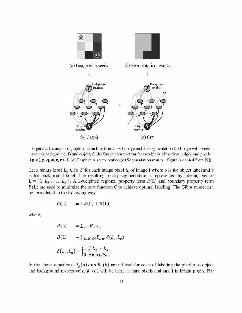
example is illustrated in Figure 2 to demonstrate the use of graph cuts segmentation.
15
Figure 2. Example of graph construction from a 3x3 image and 2D segmentation (a) Image with seeds
such as background, B and object, O (b) Graph construction for two kinds of vertices, edges and pixels i, j�, i, j,k, l, m b n (c) Graph cuts segmentation (d) Segmentation results. (figure is copied from [9]).
Let a binary label Ao b Bp, qCfor each image pixel $o of image I where o is for object label and b
is for background label. The resulting binary segmentation is represented by labeling vector r � A�,A�, …… , A|S|�. A λ-weighted regional property term t r� and boundary property term f r� are used to minimize the cost function C to achieve optimal labeling. The Gibbs model can
be formulated in the following way.
Y r� � K t r� / f r�
where,
t r� � ∑ t?. A??PS
f r� � ∑ f?,M. u A?, AM� ?,M�PΝ
uIA?, AMJ � "1 $% A? O AM0 p��-vw$�-)
In the above equations, t? p� ��� t? q� are utilized for costs of labeling the pixel p as object
and background respectively. t? p� will be large in dark pixels and small in bright pixels. For

16
neighboring pixels p,q the term f ?,M� acts as cost associated local labeling function. f ?,M� will
be large if both p and q are included either in object or background i.e. similar ; it will be small
across the object or background boundary and will be close to 0 if p and q are fully different. The
entire graph construction comprises both the n-links such as B., XC and t-links viz. B., �C , B., �C. Weights of each graph edges are employed to the graph according to Table 1. After finding a
maximum flow from s to t the minimum s-t cut problem can be solved.
Table 1. Cost terms for graph cuts segmentation [5]
Graph edge Cost Condition
n-link {p, q} B{p, q} {p, q}bN
t-link {s, p} λ · Rp (b) . b x, . y ezf� K p bO
0 p bB
t-link {p, t} λ · Rp (o) . b x, . y ezf� 0 p bO
K p bB
If an edge has non-negative capacity, a flow network can be identified. The maximum required
flow capacity of the edge from source s to . b e or from . b f to sink t is represented by the
below mentioned equation [5],
{ � 1/ ��?bS ∑ f ?,M�M: ?,M�b}
The graph cuts method is aimed to minimize the objective function i.e. energy of the image
corresponding all required labeling for the object and background seeds. The summarization of
steps used in graph cuts method can be depicted as below.
i. An edge directed graph representing size and dimension of the target segmenting
image has to be created.
ii. Object and background seeds have to be distinguished properly with formation of two
graph nodes-source s and sink t. Based on the object or the background labels, all
seeds have to be connected with either source or sinks node.
iii. According to table 1 each link of the formed graph is to be associated with suitable
edge cost.
iv. Any minimum s-t cut method is to be used which indicates the graph nodes
representing image boundaries for object and background.
v. A suitable maximum flow solution for graph optimization is to be determined for
graph cuts segmentation.
17
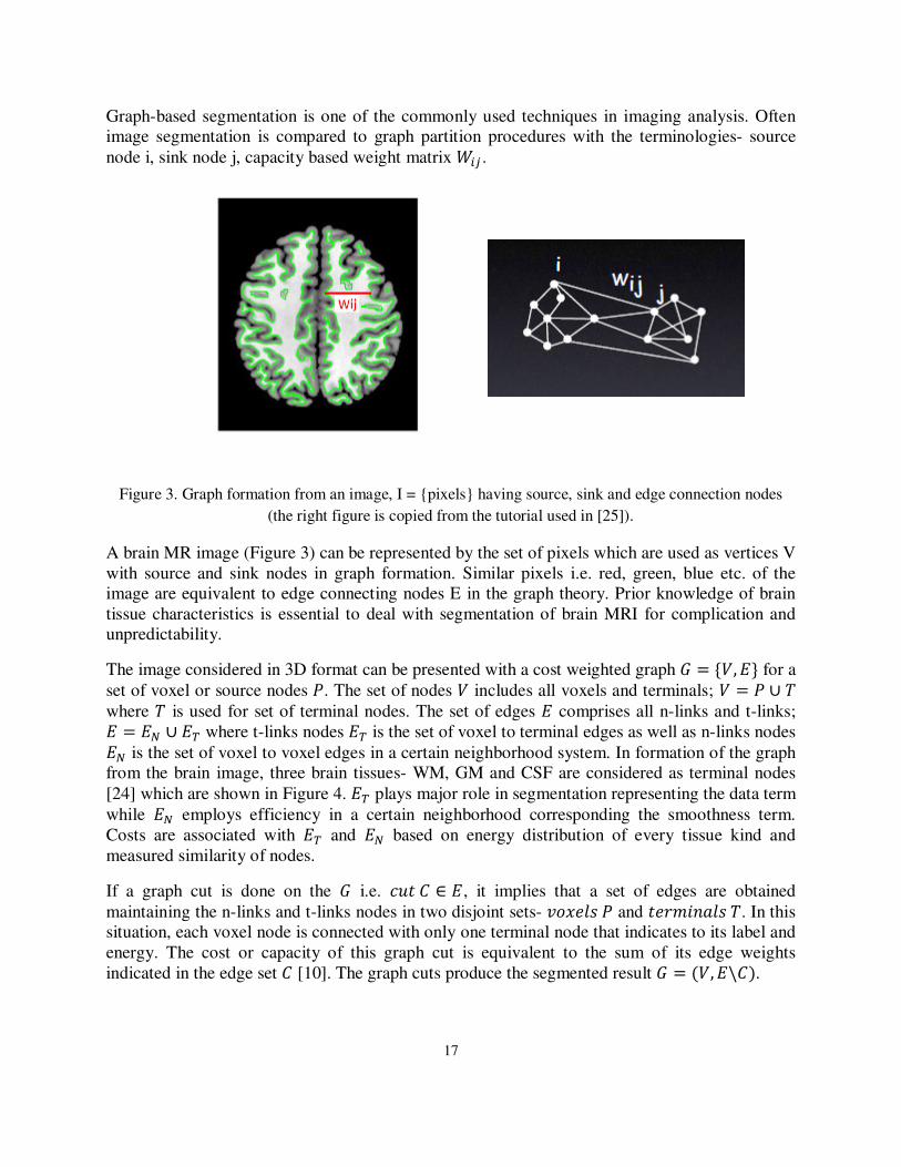
Graph-based segmentation is one of the commonly used techniques in imaging analysis. Often
image segmentation is compared to graph partition procedures with the terminologies- source
node i, sink node j, capacity based weight matrix ~�� .
Figure 3. Graph formation from an image, I = {pixels} having source, sink and edge connection nodes
(the right figure is copied from the tutorial used in [25]).
A brain MR image (Figure 3) can be represented by the set of pixels which are used as vertices V
with source and sink nodes in graph formation. Similar pixels i.e. red, green, blue etc. of the
image are equivalent to edge connecting nodes E in the graph theory. Prior knowledge of brain
tissue characteristics is essential to deal with segmentation of brain MRI for complication and
unpredictability.
The image considered in 3D format can be presented with a cost weighted graph 4 � B`, GC for a
set of voxel or source nodes �. The set of nodes ` includes all voxels and terminals; ` � � a �
where � is used for set of terminal nodes. The set of edges G comprises all n-links and t-links; G � G} a G� where t-links nodes G� is the set of voxel to terminal edges as well as n-links nodes G} is the set of voxel to voxel edges in a certain neighborhood system. In formation of the graph
from the brain image, three brain tissues- WM, GM and CSF are considered as terminal nodes
[24] which are shown in Figure 4. G� plays major role in segmentation representing the data term
while G} employs efficiency in a certain neighborhood corresponding the smoothness term.
Costs are associated with G� and G} based on energy distribution of every tissue kind and
measured similarity of nodes.
If a graph cut is done on the 4 i.e. ��� Y b G, it implies that a set of edges are obtained
maintaining the n-links and t-links nodes in two disjoint sets- �p�-�� � and �-v$���� �. In this
situation, each voxel node is connected with only one terminal node that indicates to its label and
energy. The cost or capacity of this graph cut is equivalent to the sum of its edge weights
indicated in the edge set Y [10]. The graph cuts produce the segmented result 4 � `, G\Y�.

18
Figure 4. Graph formation, � � B�, �C with three tissues-GM, WM and CSF for brain MRI segmentation
(the figure is copied from [24]).
3.2 Min-cut/max-flow algorithm for graph cuts
The energy minimization procedures for machine vision and automated image segmentation are
explored by Boykov and Kolmogorov in [6]. Based on augmenting paths, the min-cut/max flow
algorithm is presented with two reusable and non-overlapping search trees- S: from source s and
T: from sink t. Tree S has the direction of non-saturation from parent node to children and tree T
has non-saturation from children to parent node. There can be active or passive node in S or T
based on outer border and internal border respectively. Free nodes are those who are not in S or
T considering the conditions: � c `, � b �, � c `, � b � ��� �g� � �. The graphical
illustration of this new algorithm is shown in figure 4.
Figure 5. Example of the min-cut/max-flow algorithm in graph cuts segmentation (the figure is copied
from [6]).
Red nodes indicate search tree S, blue nodes represent search tree T and yellow line is for the
path from the source s to sink t. Free nodes are represented as black circle while active node is by
A and passive node is by P in Figure 5. The combination of minimum s-t cut and maximum flow
optimizations is accomplished with three steps-growth, augmentation and adoption in the
segmentation procedure.
19
3.3 Normalized graph cut
The normalized cut is a global criterion for segmenting graph used in image data rather than
focusing on local features and consistencies [18]. This algorithm is used as a criterion to measure
total dissimilarity between various groups and total similarity within the groups. This technique
can be applied on static general and medical imaging. The normalized cut, ���� ., X� described
as balanced cut is presented with the equation mentioned below.
���� ., X� � ��� ., X�. ��_� ?� / �
�_� M�� where
��� ., X� � ∑ ��,��b?,�bM
�p��- p% �-�: �p� .� �H�� , . � `�b?
�p��- p% �-�: �p� X� �H��, X � `�bM
7-�v-- p% �p�-: �� � H����
�$$��v$�! ��v$�: � � *���,
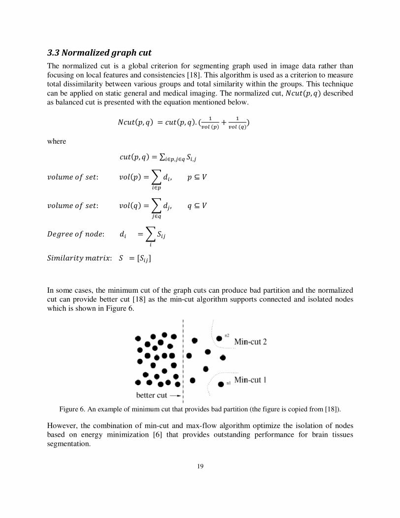
In some cases, the minimum cut of the graph cuts can produce bad partition and the normalized
cut can provide better cut [18] as the min-cut algorithm supports connected and isolated nodes
which is shown in Figure 6.
Figure 6. An example of minimum cut that provides bad partition (the figure is copied from [18]).
However, the combination of min-cut and max-flow algorithm optimize the isolation of nodes
based on energy minimization [6] that provides outstanding performance for brain tissues
segmentation.

20
3.4 Brain image segmentation using a combination of softwares
3.4.1 The MRIcroN software [21]
MRIcroN is widely used public software to view image of the neuroimaging informatics
technology initiative (NIfTI) format. To convert the digital imaging and communications in
medicine (DICOM) standard images into NIfTI and non-parametric statistical mapping (NPM)
formats, MRIcroN software is applied with dcm2nii parameter. Multiple layers of images can be
loaded easily in this software along with drawing volumes of interests and generating volume
renderings. Several color schemes can be chosen for every layer. A series of slices of the
currently open image in the 3D format can be seen with multi-slice windows option. This
software can be downloaded from the link provided in [21] and installation instruction is
provided.
3.4.2 FMRIB Software Library (FSL) [22]
Different kinds of analysis tools for brain imaging data such as MRI, functional MRI (fMRI),
diffusion tensor imaging (DTI) etc. can be investigated by publicly available FMRIB software
library (FSL). In structural MRI, FSL is used with several tools viz. brain extraction tool (BET),
FMRIB’s automated segmentation tool (FAST), FMRIB’s linear image registration tool
(FLIRT), FMRIB’s nonlinear image registration tool (FNIRT) etc. BET and FAST are the
predominant ones to analyze brain image segmentation especially brain and non-brain
components are segmented by BET. The FSL software can be downloaded from the link
provided in [22] and is easy to install in the personal computer.
21
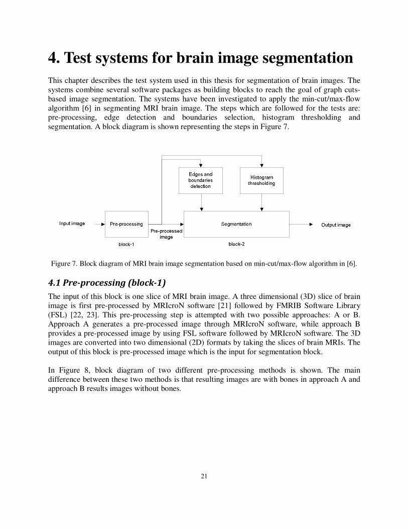
4. Test systems for brain image segmentation
This chapter describes the test system used in this thesis for segmentation of brain images. The
systems combine several software packages as building blocks to reach the goal of graph cuts-
based image segmentation. The systems have been investigated to apply the min-cut/max-flow
algorithm [6] in segmenting MRI brain image. The steps which are followed for the tests are:
pre-processing, edge detection and boundaries selection, histogram thresholding and
segmentation. A block diagram is shown representing the steps in Figure 7.
Figure 7. Block diagram of MRI brain image segmentation based on min-cut/max-flow algorithm in [6].
4.1 Pre-processing (block-1)
The input of this block is one slice of MRI brain image. A three dimensional (3D) slice of brain
image is first pre-processed by MRIcroN software [21] followed by FMRIB Software Library
(FSL) [22, 23]. This pre-processing step is attempted with two possible approaches: A or B.
Approach A generates a pre-processed image through MRIcroN software, while approach B
provides a pre-processed image by using FSL software followed by MRIcroN software. The 3D
images are converted into two dimensional (2D) formats by taking the slices of brain MRIs. The
output of this block is pre-processed image which is the input for segmentation block.
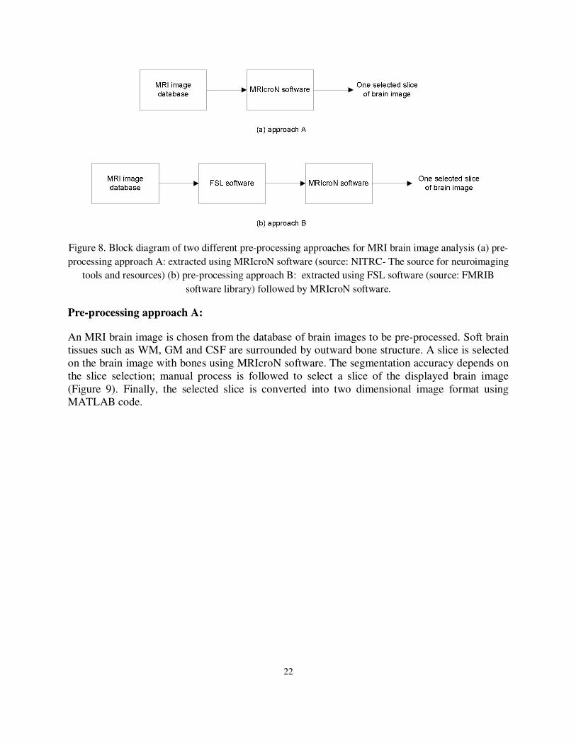
In Figure 8, block diagram of two different pre-processing methods is shown. The main
difference between these two methods is that resulting images are with bones in approach A and
approach B results images without bones.
22
Figure 8. Block diagram of two different pre-processing approaches for MRI brain image analysis (a) pre-
processing approach A: extracted using MRIcroN software (source: NITRC- The source for neuroimaging
tools and resources) (b) pre-processing approach B: extracted using FSL software (source: FMRIB
software library) followed by MRIcroN software.
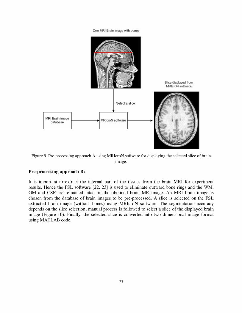
Pre-processing approach A:
An MRI brain image is chosen from the database of brain images to be pre-processed. Soft brain
tissues such as WM, GM and CSF are surrounded by outward bone structure. A slice is selected
on the brain image with bones using MRIcroN software. The segmentation accuracy depends on
the slice selection; manual process is followed to select a slice of the displayed brain image
(Figure 9). Finally, the selected slice is converted into two dimensional image format using
MATLAB code.
23
Figure 9. Pre-processing approach A using MRIcroN software for displaying the selected slice of brain
image.
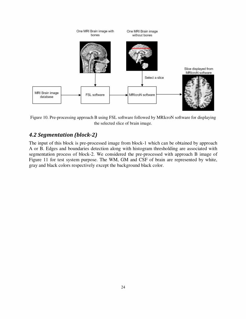
Pre-processing approach B:
It is important to extract the internal part of the tissues from the brain MRI for experiment
results. Hence the FSL software [22, 23] is used to eliminate outward bone rings and the WM,
GM and CSF are remained intact in the obtained brain MR image. An MRI brain image is
chosen from the database of brain images to be pre-processed. A slice is selected on the FSL
extracted brain image (without bones) using MRIcroN software. The segmentation accuracy
depends on the slice selection; manual process is followed to select a slice of the displayed brain
image (Figure 10). Finally, the selected slice is converted into two dimensional image format
using MATLAB code.
24
Figure 10. Pre-processing approach B using FSL software followed by MRIcroN software for displaying
the selected slice of brain image.
4.2 Segmentation (block-2)
The input of this block is pre-processed image from block-1 which can be obtained by approach
A or B. Edges and boundaries detection along with histogram thresholding are associated with
segmentation process of block-2. We considered the pre-processed with approach B image of
Figure 11 for test system purpose. The WM, GM and CSF of brain are represented by white,
gray and black colors respectively except the background black color.

25
Figure 11. Pre-processed (using approach B) MRI image: Gray matter (GM), white matter (WM) and
Cerebrospinal Fluid (CSF).
In the edge detection step, a two-dimensional (3x3) median filter is chosen to minimize the cost
function of the image data and to reduce noise and preserve edges simultaneously. Every output
pixel includes the median value in the 3 by 3 neighborhood around the corresponding pixel in the
input brain image. To find the accurate edges, ‘canny’ detection method is used to construct the
graph Gst on the filtered image as it finds edges by looking for local maxima of the gradient
calculating the derivative (Figure 12). This method uses two main thresholds: detecting strong
and weak edges along with the output of weak edges if they are connected to strong edges. The
edge detected image has to be much smooth and intensity oriented for both connected and non-
connected components. Hence, we used full two dimensional convolution of the edge detected
image to make it smooth for both connected and non-connected components of different
intensity and energy levels. Convolution is done for finding the connected (active or passive
nodes) components and non-connected (free nodes) components in the search trees S and T, and
costs are assigned on the edges of Gst. The boundaries of the brain tissues are detected also based
on the different pixel intensity levels to apply in further segmentation process. Both the
connected and non-connected components of the image like WM, GM or CSF are important to
analyze for segmentation. The image is converted into red-green-blue (RGB) matrix format for
viewing distinctly all connected and non- connected nodes.
26
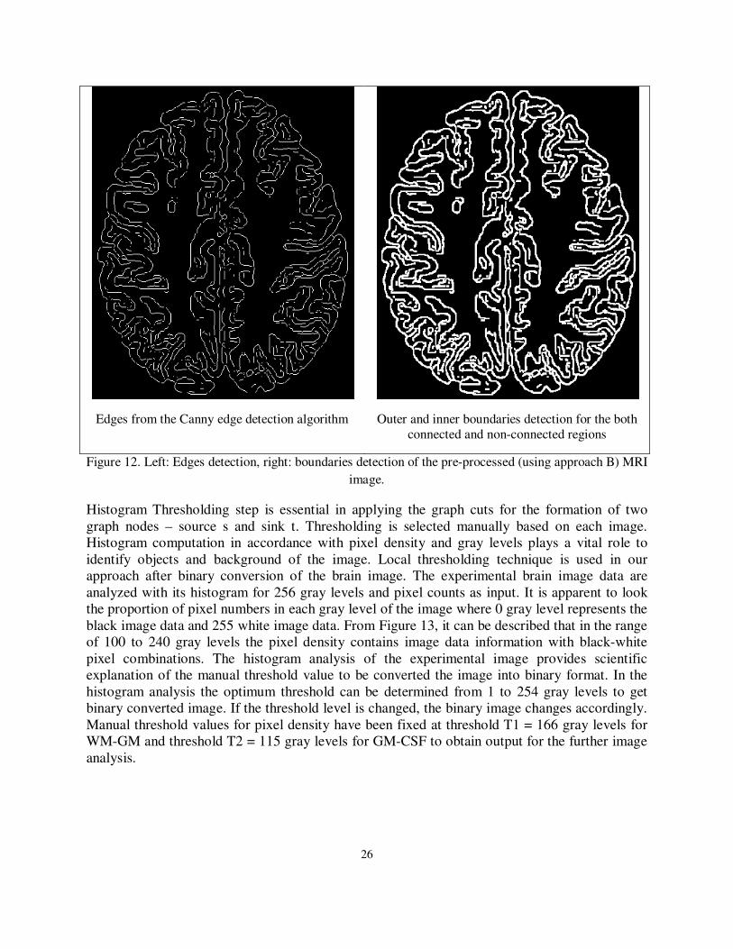
Edges from the Canny edge detection algorithm
Outer and inner boundaries detection for the both
connected and non-connected regions
Figure 12. Left: Edges detection, right: boundaries detection of the pre-processed (using approach B) MRI
image.
Histogram Thresholding step is essential in applying the graph cuts for the formation of two
graph nodes – source s and sink t. Thresholding is selected manually based on each image.
Histogram computation in accordance with pixel density and gray levels plays a vital role to
identify objects and background of the image. Local thresholding technique is used in our
approach after binary conversion of the brain image. The experimental brain image data are
analyzed with its histogram for 256 gray levels and pixel counts as input. It is apparent to look
the proportion of pixel numbers in each gray level of the image where 0 gray level represents the
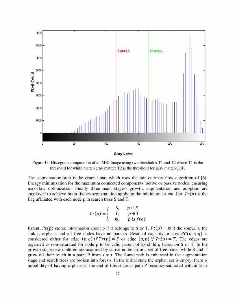
black image data and 255 white image data. From Figure 13, it can be described that in the range
of 100 to 240 gray levels the pixel density contains image data information with black-white
pixel combinations. The histogram analysis of the experimental image provides scientific
explanation of the manual threshold value to be converted the image into binary format. In the
histogram analysis the optimum threshold can be determined from 1 to 254 gray levels to get
binary converted image. If the threshold level is changed, the binary image changes accordingly.
Manual threshold values for pixel density have been fixed at threshold T1 = 166 gray levels for
WM-GM and threshold T2 = 115 gray levels for GM-CSF to obtain output for the further image
analysis.
27
Figure 13. Histogram computation of an MRI image using two thresholds T1 and T2 where T1 is the
threshold for white matter-gray matter; T2 is the threshold for gray matter-CSF.
The segmentation step is the crucial part which uses the min-cut/max flow algorithm of [6].
Energy minimization for the maximum connected components (active or passive nodes) ensuring
max-flow optimization. Finally three main stages- growth, augmentation and adoption are
employed to achieve brain tissues segmentation applying the minimum s-t cut. Let, �v .� is the
flag affiliated with each node p in search trees S and T,
�v .� � � �, . b � �, . b � h, . $� %v--) Parent, �� .� stores information about p if it belongs to S or T. �� .� � h if the source s, the
sink t, orphans and all free nodes have no parents. Residual capacity or cost tY . � X� is
considered either for edge ., X� $% �v .� � � or edge X, .� $% �v .� � �. The edges are
regarded as non-saturated for node p to be valid parent of its child q based on S or T. In the
growth stage new children are acquired by active nodes from a set of free nodes while S and T
grow till their touch in a path, P from s to t. The found path is enhanced in the augmentation
stage and search trees are broken into forests. In the initial state the orphan set is empty; there is
possibility of having orphans in the end of this stage as path P becomes saturated with at least
28
one edge. In the adoption stage, S and T are restored by processing all orphan nodes, O. In the
same search tree, each node p tries to identify new and valid parent; p becomes children of a new
parent or becomes free node.
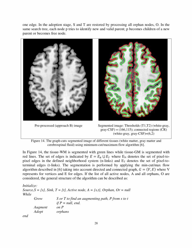
Pre-processed (approach B) image
Segmented image: Thresholds (T1,T2) (white-gray,
gray-CSF) = (166,115); connected regions (CR)
(white-gray, gray-CSF)=(6,2)
Figure 14. The graph-cuts segmented image of different tissues (white matter, gray matter and
cerebrospinal fluid) using minimum-cut/maximum flow algorithm [6].
In Figure 14, the tissue-WM is segmented with green lines while tissue-GM is segmented with
red lines. The set of edges is indicated by G � G} zG� where EN denotes the set of pixel-to-
pixel edges in the defined neighborhood system (n-links) and ET denotes the set of pixel-to-
terminal edges (t-links). The segmentation is performed by applying the min-cut/max flow
algorithm described in [6] taking into account directed and connected graph, 4 � `, G� where V
represents for vertices and E for edges. If the list of all active nodes, A and all orphans, O are
considered, the general structure of the algorithm can be described as:
Initialize:
Source,S = {s}, Sink, T = {t}, Active node, A = {s,t}, Orphan, Or = null
While
Grow S or T to find an augmenting path, P from s to t
if P = null, end.
Augment on P
Adopt orphans
end
29
Active node helps the tree to grow by searching adjacent non-saturated nodes and acquiring new
children from a set of free nodes while the passive node cannot grow as blocked by other nodes
of the same tree. In this growth stage, newly acquired node becomes active member of the
corresponding search tree. The certain active node becomes passive after finishing exploration of
all the neighbors. The growth stage will be ceased if an active node finds a neighbor comprised
of opposite search tree.
The path found in the growth stage is followed by the active nodes and is augmented through the
excavated route which represents the augmentation stage. The input of this stage is a path P from
s to t. The augmentation phase can split the search trees into forest. In the forest, s and t are the
roots of the mentioned search trees while other orphans constitute roots of all other trees.
Adoption stage is used in our graph-cuts algorithm to restore the single tree structure of sets S
and T with specific roots in source s and sink t. Each orphan is helped to find valid parent who
will be in the same set S or T and connected through non-saturated edges. The orphan will be
free node if there is no valid & qualifying parent found. In this way, if no orphans are left to be
explored, the adoption stage is terminated and search tree S and T are formed.
In the brain tissues segmentation by the graph cuts method, three of the mentioned stages are
iteratively performed and image data can be segmented based on minimum cut and maximum
flow process. Let, � x|e�is the probability of a particular gray level corresponding to the image
object and � x|f� is the probability of a particular gray level corresponding to the image
background. The regional cost, Rp and the boundary cost B(p,q) are determined with the
following equations [5].
t? pq+-��, p� � � ln�Ix?|eJ t? q����vp���, q� � � ln�Ix?|fJ
f ., X� � exp �� IST�SUJV��V � . ��?,M�
Here, the distance between pixels p,q is denoted by �., X�. σ is represented as expected intensity
variation for the object and background of the brain image. If the image values within small
differences (Ex? � xME � 1) for object or background, the boundary cost is high. In boundary
locations positioned at Ex? � xME & 1, cost B(p,q) is low.
Discussion: variable thresholding in histogram based on local statistics:
Image thresholding enjoys a central position in application of image segmentation for its
intuitive properties and simplicity of implementation. Global thresholding, optimum global
thresholding with Otsu’s method, image smoothing, image edges, variable thresholding based on
local statistics and thresholding with moving averages are commonly used for image
thresholding process [1].
30
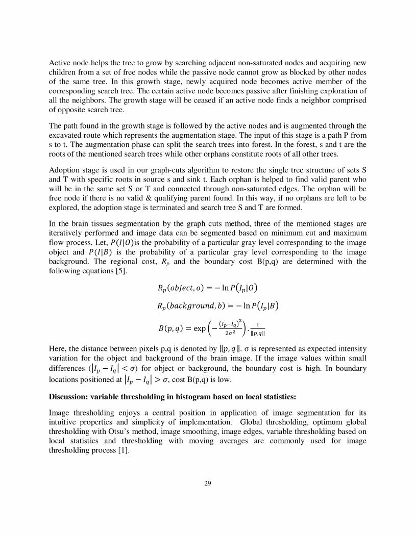
In applying the min-cut/max-flow algorithm of graph cuts image segmentation, variable
thresholding based on local statistics is used. If the background illumination of the image is non-
uniformed, global thresholding methods typically fail. In that case variable thresholding is used
to compensate for irregularities in illumination or in cases where there is more than one
dominant object intensity. A threshold value at every point (x, y) in the image is computed for
local statistics technique based on one or more specified properties of the pixels in a
neighborhood of (x, y). We determined the basic approach to local thresholding using the
standard deviation and mean of the pixels in a neighborhood of every point in the brain MR
image because they are descriptors of local contrast and average intensity. The images below
(Figure 15) illustrate some Matlab simulation results for different thresholdings in applying the
graph cuts segmentation.
Pre-processed (approach B) image
Segmented image: Thresholds (T1,T2) (white-
gray, gray-CSF) = (115, 64); connected regions
(CR) (white-gray, gray-CSF)=(2,1)

31
(T1,T2)=(166,115), CR=(6,2)
(T1,T2)=(191,140); CR=(10,6)
(T1,T2)=(217,166); CR=(22,6)
(T1,T2)=(230,179); CR=(58,11)
Figure 15. Segmented results from a pre-processed image (approach B) using different thresholds.
32
In 50 and 100 gray levels of variable thresholding, local statistics provide WM, GM
segmentation to a little extent because of poor contrast and intensity. If the local threshold value
exceeds 240 gray levels, the brain tissue segmentation level is decreased. Hence, the threshold
values can be chosen in the range of 150-200 gray levels to obtain acceptable segmentation
results with the min-cut/max-flow algorithm of graph cuts. Binary threshold varies the maximum
connected energy levels which also reflect on augmentation and adoption stages of graph cuts.
Threshold values are selected manually for the image slice especially for WM, GM and CSF
tissues segmentation. Threshold T1 provides the number of connected regions between WM and
GM in certain gray level and threshold T2 remarks the number of connected regions between
GM and CSF in a gray level.
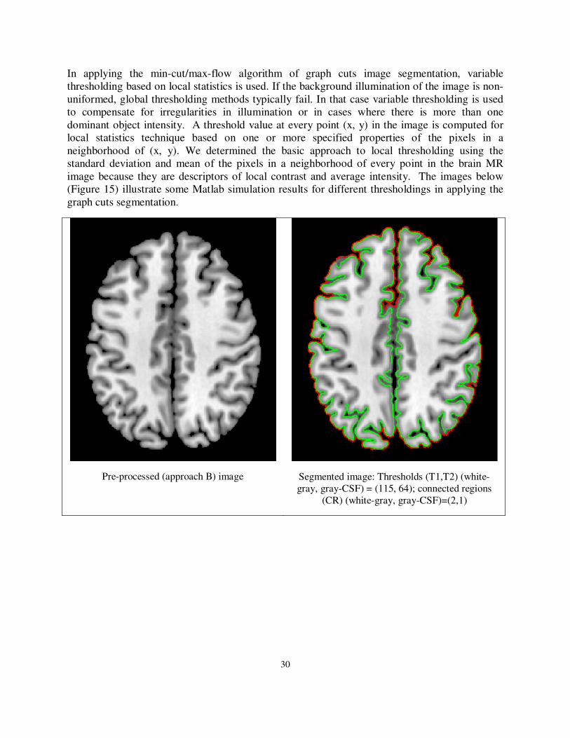
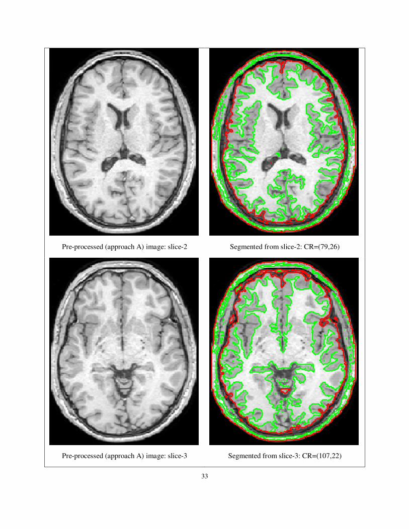
Discussion: pre-processing A (MRIcroN software) approach in segmentation
The pre-processing stage of brain MR image is important to perform analysis and segmentation
appropriately. The brain MR images can be captured with human head’s bone structure with
MRIcroN software. Randomly five slices of one brain MR image have been chosen through the
MRIcroN software to conduct test of our Matlab simulated program for the graph cuts. Brain
tissues are segmented along with the bone structure which is not expected in the further analysis.
Effects of pre-processed (approach A) brain MR images are illustrated in Figure 16 using five
different image slices (slices 1-5).
Pre-processed (approach A) image: slice-1
Segmented from slice-1: connected regions (CR)
(white-gray, gray-CSF)=(86,25)
33
Pre-processed (approach A) image: slice-2
Segmented from slice-2: CR=(79,26)
Pre-processed (approach A) image: slice-3
Segmented from slice-3: CR=(107,22)

34
Pre-processed (approach A) image: slice-4
Segmented from slice-4: CR=(123,22)
Pre-processed (approach A) image: slice-5
Segmented from slice-5: CR=(89,27)
Figure 14. Segmentation results using pre-processed (approach A) MRI image with MRIcroN software.
Same thresholds are used for these 5 images: (T1,T2)=(191,115) ,where T1 is the threshold for white
matter-gray matter; T2 is the threshold for gray matter-CSF.
35
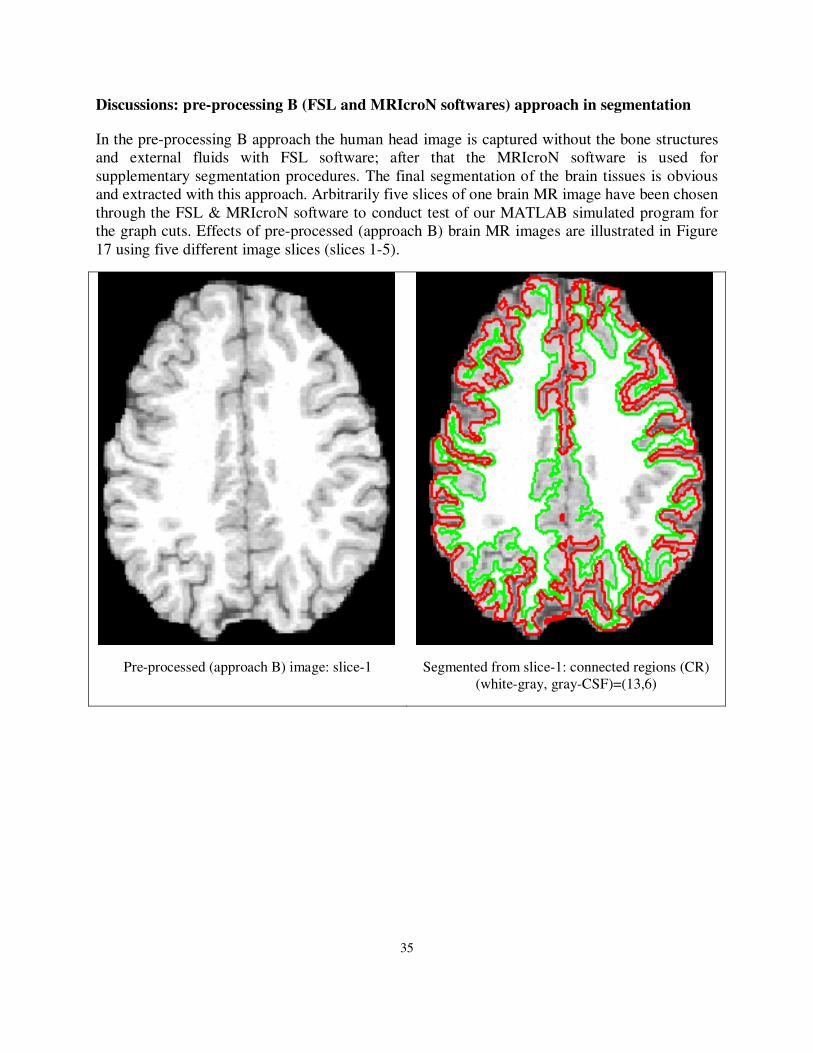
Discussions: pre-processing B (FSL and MRIcroN softwares) approach in segmentation
In the pre-processing B approach the human head image is captured without the bone structures
and external fluids with FSL software; after that the MRIcroN software is used for
supplementary segmentation procedures. The final segmentation of the brain tissues is obvious
and extracted with this approach. Arbitrarily five slices of one brain MR image have been chosen
through the FSL & MRIcroN software to conduct test of our MATLAB simulated program for
the graph cuts. Effects of pre-processed (approach B) brain MR images are illustrated in Figure
17 using five different image slices (slices 1-5).
Pre-processed (approach B) image: slice-1
Segmented from slice-1: connected regions (CR)
(white-gray, gray-CSF)=(13,6)
36
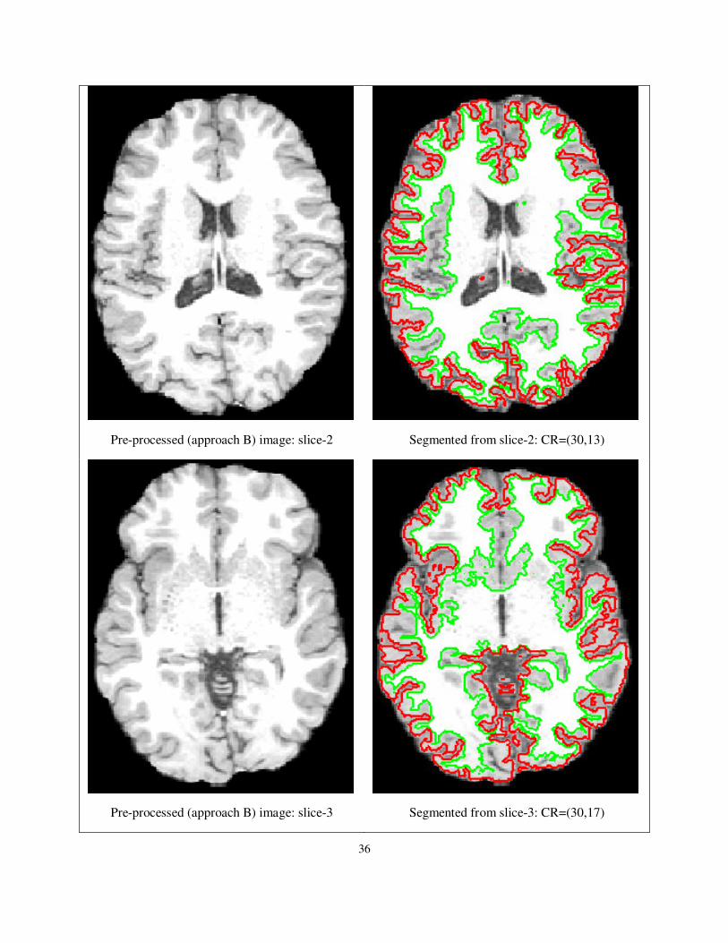
Pre-processed (approach B) image: slice-2
Segmented from slice-2: CR=(30,13)
Pre-processed (approach B) image: slice-3
Segmented from slice-3: CR=(30,17)
37
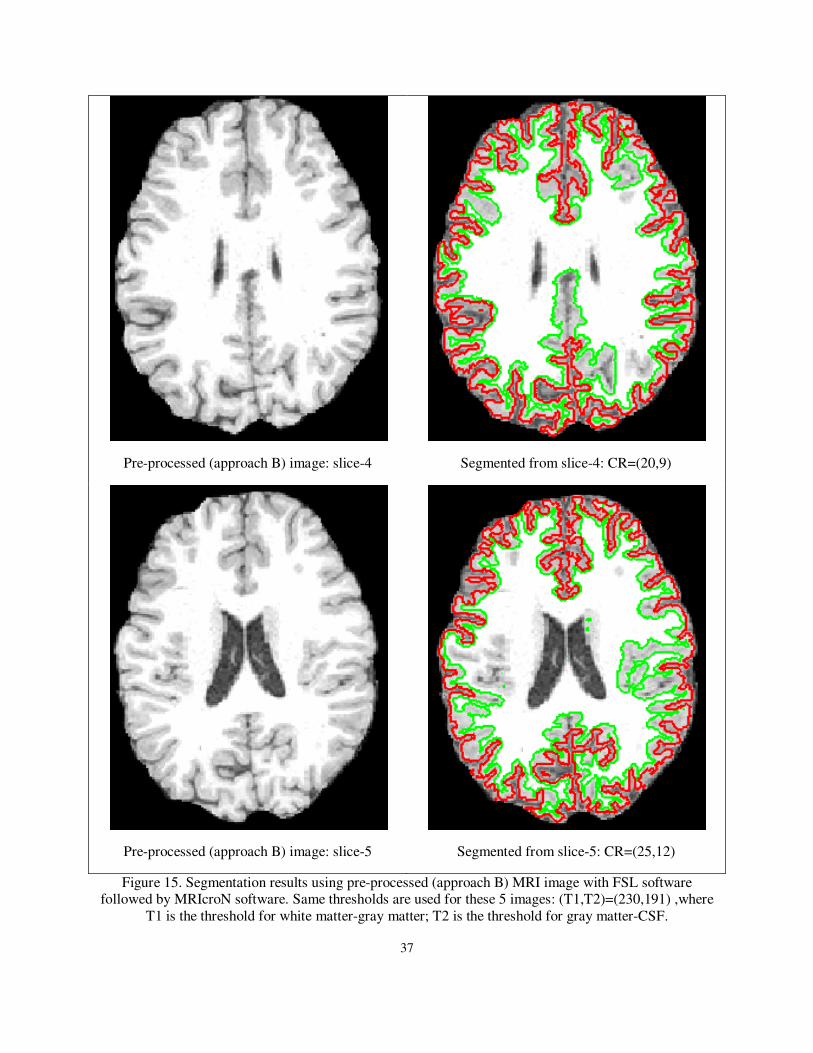
Pre-processed (approach B) image: slice-4
Segmented from slice-4: CR=(20,9)
Pre-processed (approach B) image: slice-5
Segmented from slice-5: CR=(25,12)
Figure 15. Segmentation results using pre-processed (approach B) MRI image with FSL software followed by MRIcroN software. Same thresholds are used for these 5 images: (T1,T2)=(230,191) ,where
T1 is the threshold for white matter-gray matter; T2 is the threshold for gray matter-CSF.
38
5. Experimental Results
Medical image segmentation for brain MRI is an emerging field with upcoming new techniques
and algorithms. We performed experiments with some existing algorithms used in the graph cuts
method on the synthetic brain MR images. MATLAB simulation results with the min-cut/max-
flow algorithm provide better segmentation outputs comparing with the normalized cut methods.
This chapter is organized for the simulated results with existing MATLAB tools by the
normalized cut and then our approach to implement the min-cut/max-flow algorithm and
comparison of our implementation with the normalized cut with two techniques. We initially
segmented the brain MR image applying the normalized cut algorithm with available simulation
tools; finally the segmentation is done applying the min-cut/max-flow algorithm with our own
MATLAB programming codes.
The synthetic images used in our experiments were collected from the MRI scans of adult brains
with general intrinsic tissue variation. T2-weighted MRI has better contrast than T1-weighted
one [24] because of long echo time (TE) and long repetition time (TR); but T1-weighted BRI
brain image is prudent to analyze in fundamental research. Hence, axial T1-weighted images
scanned with spin-echo pulse sequence were used in the simulation having long partial volume
effect and low contrast to noise ratio. The voxel of the image was selected in 0.30 � 0.30 � 2.5 for MRIcroN software which was sliced and converted into 2D form by
MATLAB. Segmentation of GM and WM were considered; the skull and other brain tissues
were not included in applying the min-cut/max flow algorithm for simplicity. 10 different slices
of human brain images have been tested where 5 slices were pre-processed using approach A
and another 5 slices by approach B. Thresholding change impacts the segmentation result which
is described in earlier section.
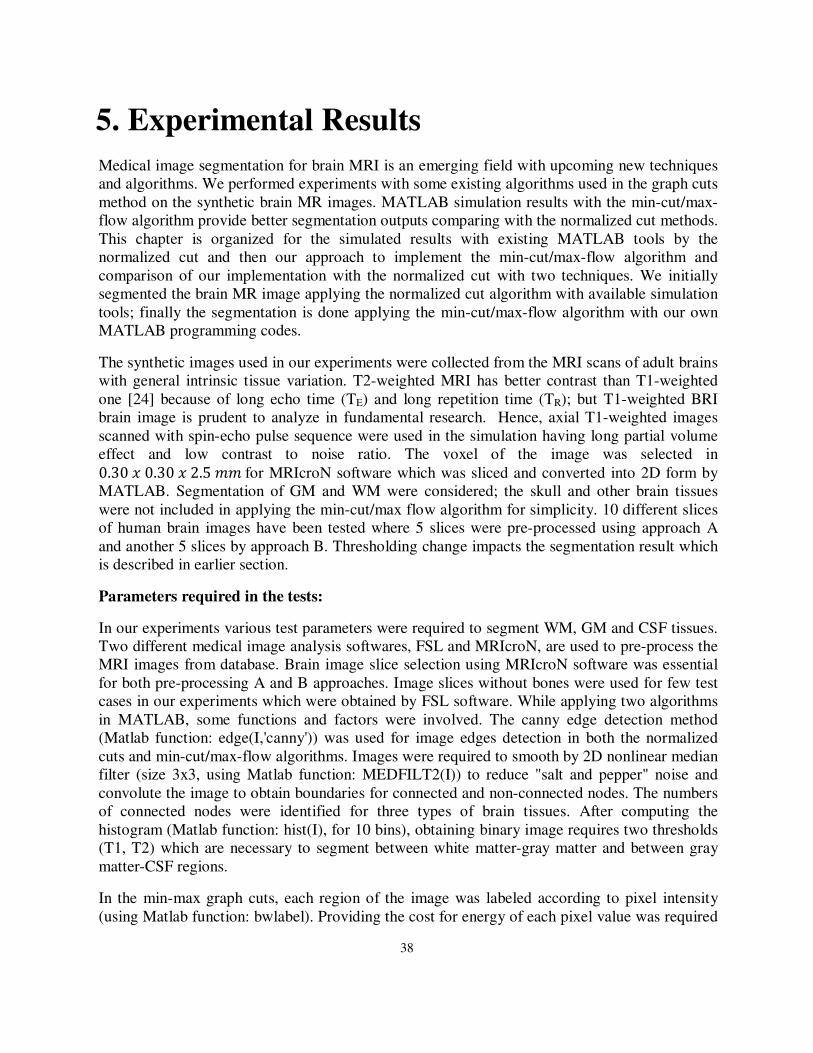
Parameters required in the tests:
In our experiments various test parameters were required to segment WM, GM and CSF tissues.
Two different medical image analysis softwares, FSL and MRIcroN, are used to pre-process the
MRI images from database. Brain image slice selection using MRIcroN software was essential
for both pre-processing A and B approaches. Image slices without bones were used for few test
cases in our experiments which were obtained by FSL software. While applying two algorithms
in MATLAB, some functions and factors were involved. The canny edge detection method
(Matlab function: edge(I,'canny')) was used for image edges detection in both the normalized
cuts and min-cut/max-flow algorithms. Images were required to smooth by 2D nonlinear median
filter (size 3x3, using Matlab function: MEDFILT2(I)) to reduce "salt and pepper" noise and
convolute the image to obtain boundaries for connected and non-connected nodes. The numbers
of connected nodes were identified for three types of brain tissues. After computing the
histogram (Matlab function: hist(I), for 10 bins), obtaining binary image requires two thresholds
(T1, T2) which are necessary to segment between white matter-gray matter and between gray
matter-CSF regions.
In the min-max graph cuts, each region of the image was labeled according to pixel intensity
(using Matlab function: bwlabel). Providing the cost for energy of each pixel value was required
39
to find maximum flow of the connected regions. Minimum cut was achieved after finding the
maximum flow using pixels’ growth, augmentation and adoption in search trees S and T.
Properties of image regions were investigated to attain min-cut and applying graph cuts
segmentation. Computational time in second was checked for segmentation of each image slice
in two algorithms. The number of segments was selected manually in the normalized cut
algorithm whereas threshold values were selected manually for the min-cut/max-flow algorithm.
5.1 Brain image segmentation using the normalized cut algorithm in [18]
The normalized cut with prior application to graph cuts approach [18] has been used initially for
our brain MR image segmentation experiment with the existing MATLAB simulation tools [25].
The normalized cuts approach aimed at extracting global impression of an image rather than
focusing on local features and consistencies.
Based on the grouping algorithm in [25], brain MR image segmentation has been done with two
main criteria viz. marked segment boundaries and segmentation numbers. The normalized cuts
with marked segment boundaries technique has much complexity, computational time and the
output segmentation visual quality is in the acceptable range. But the segmentation number for
normalized cuts provide inacceptable visual quality image for brain MRI. If number of
segmentation is increased, the quality becomes worse rather performing efficient segmentation.
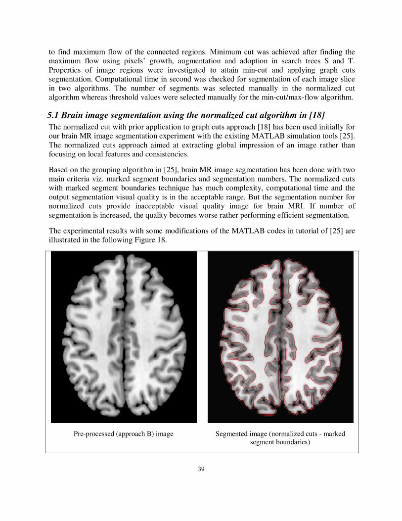
The experimental results with some modifications of the MATLAB codes in tutorial of [25] are
illustrated in the following Figure 18.
Pre-processed (approach B) image
Segmented image (normalized cuts - marked segment boundaries)
40
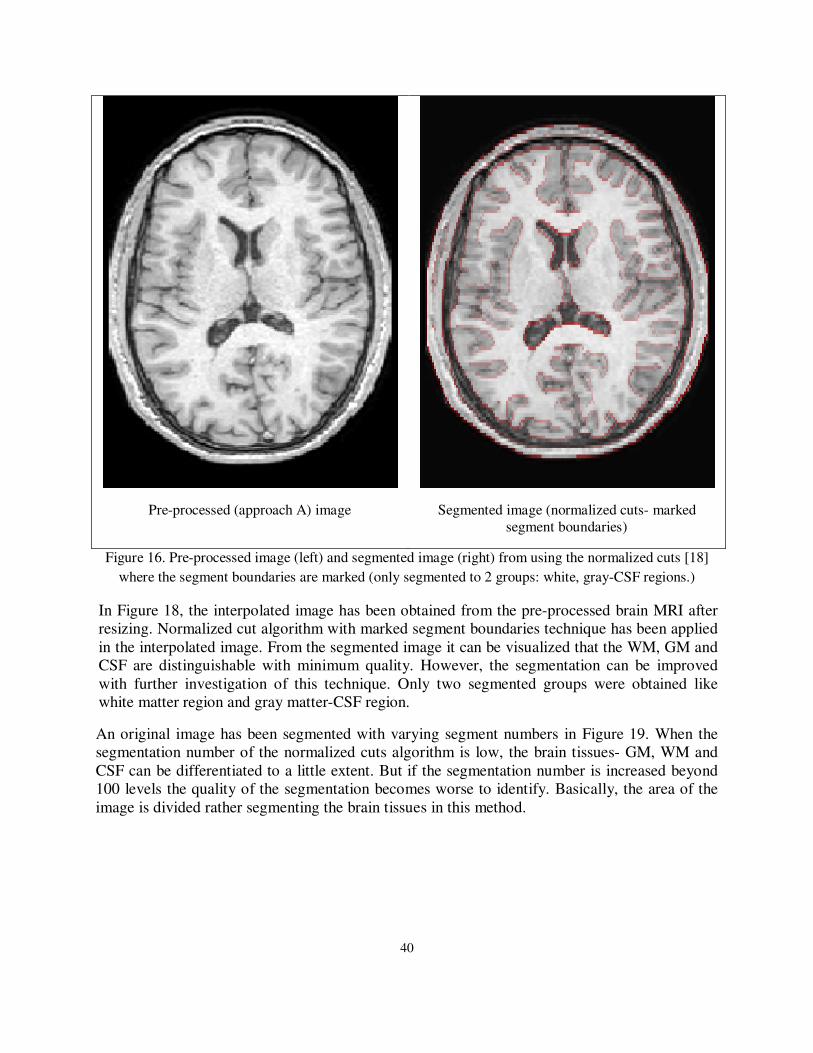
Pre-processed (approach A) image
Segmented image (normalized cuts- marked
segment boundaries)
Figure 16. Pre-processed image (left) and segmented image (right) from using the normalized cuts [18]
where the segment boundaries are marked (only segmented to 2 groups: white, gray-CSF regions.)
In Figure 18, the interpolated image has been obtained from the pre-processed brain MRI after
resizing. Normalized cut algorithm with marked segment boundaries technique has been applied
in the interpolated image. From the segmented image it can be visualized that the WM, GM and
CSF are distinguishable with minimum quality. However, the segmentation can be improved
with further investigation of this technique. Only two segmented groups were obtained like
white matter region and gray matter-CSF region.
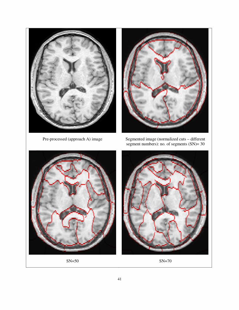
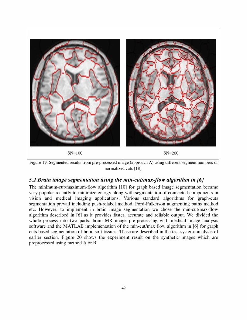
An original image has been segmented with varying segment numbers in Figure 19. When the
segmentation number of the normalized cuts algorithm is low, the brain tissues- GM, WM and
CSF can be differentiated to a little extent. But if the segmentation number is increased beyond
100 levels the quality of the segmentation becomes worse to identify. Basically, the area of the
image is divided rather segmenting the brain tissues in this method.
41
Pre-processed (approach A) image
Segmented image (normalized cuts – different segment numbers): no. of segments (SN)= 30
SN=50
SN=70
42
SN=100
SN=200
Figure 19. Segmented results from pre-processed image (approach A) using different segment numbers of
normalized cuts [18].
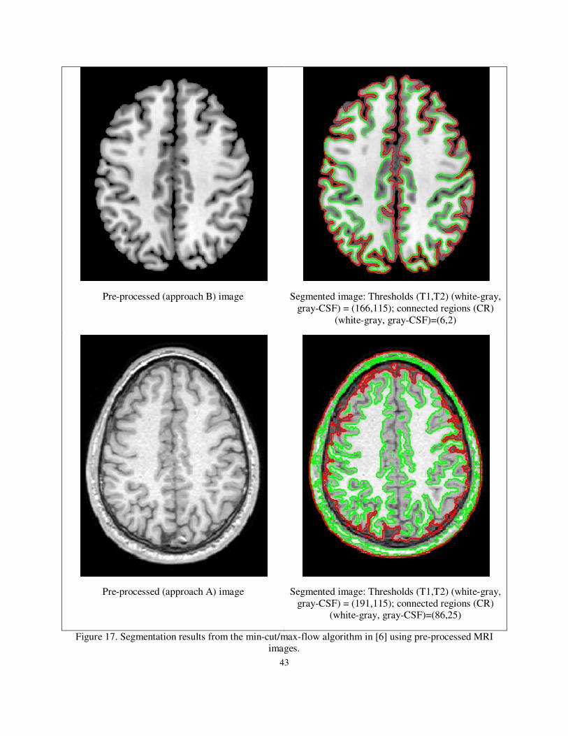
5.2 Brain image segmentation using the min-cut/max-flow algorithm in [6]
The minimum-cut/maximum-flow algorithm [10] for graph based image segmentation became
very popular recently to minimize energy along with segmentation of connected components in
vision and medical imaging applications. Various standard algorithms for graph-cuts
segmentation prevail including push-relabel method, Ford-Fulkerson augmenting paths method
etc. However, to implement in brain image segmentation we chose the min-cut/max-flow
algorithm described in [6] as it provides faster, accurate and reliable output. We divided the
whole process into two parts: brain MR image pre-processing with medical image analysis
software and the MATLAB implementation of the min-cut/max flow algorithm in [6] for graph
cuts based segmentation of brain soft tissues. These are described in the test systems analysis of
earlier section. Figure 20 shows the experiment result on the synthetic images which are
preprocessed using method A or B.
43
Pre-processed (approach B) image
Segmented image: Thresholds (T1,T2) (white-gray,
gray-CSF) = (166,115); connected regions (CR)
(white-gray, gray-CSF)=(6,2)
Pre-processed (approach A) image
Segmented image: Thresholds (T1,T2) (white-gray,
gray-CSF) = (191,115); connected regions (CR) (white-gray, gray-CSF)=(86,25)
Figure 17. Segmentation results from the min-cut/max-flow algorithm in [6] using pre-processed MRI images.

44
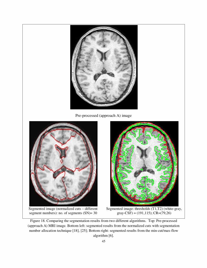
The normalized cut is performed after image interpolation and brightness minimization. It
produced poor segmentation results for brain tissues (considering only GM) where much
flexibility and accuracy are required. The graph cuts method applying the min-cut/max-flow
algorithm produced significant outputs. The segmentation results found with the normalized cut
algorithm using segmentation number 30 is compared with the min-cut/max-flow algorithm with
threshold values (T1,T2)=(191,115) for pre-processing approach A in Figure 21 and
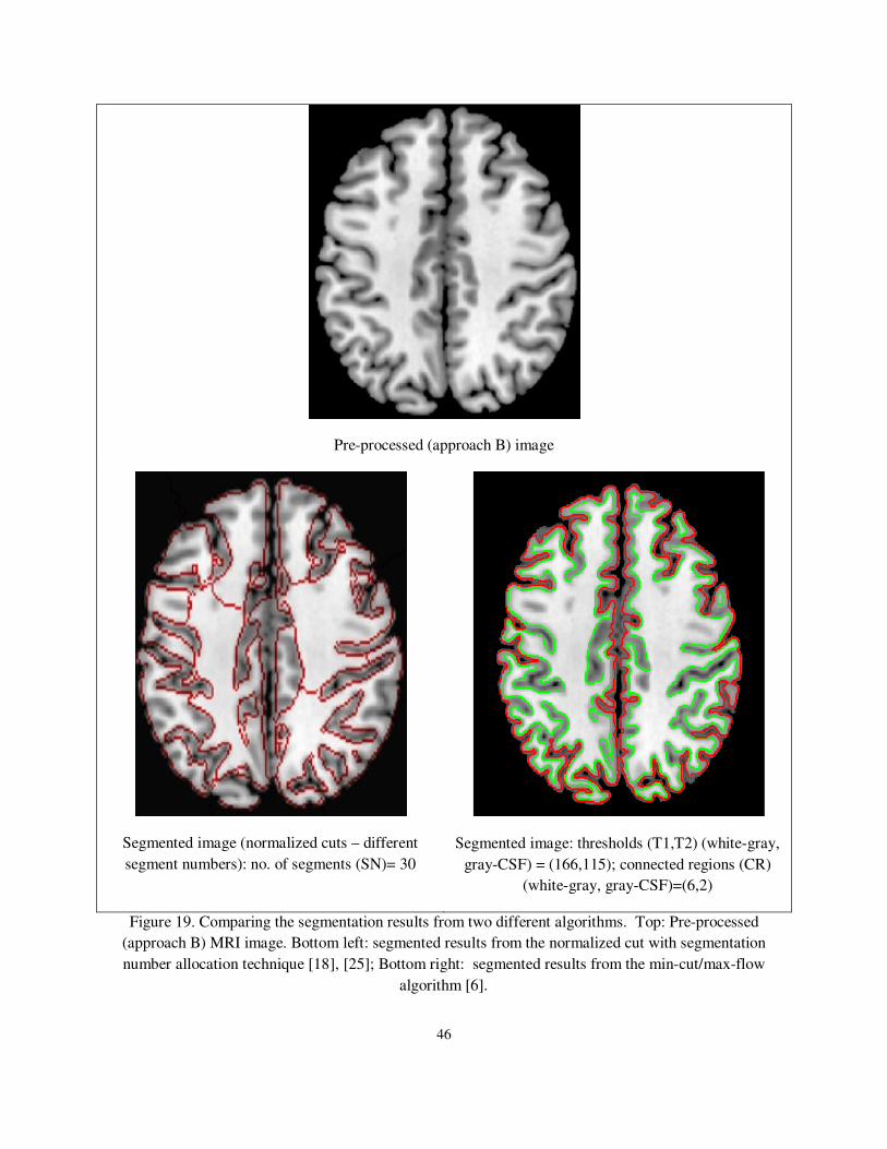
(T1,T2)=(166,115) for pre-processing approach B in Figure 22.
45
Pre-processed (approach A) image
Segmented image (normalized cuts – different
segment numbers): no. of segments (SN)= 30 Segmented image: thresholds (T1,T2) (white-gray,
gray-CSF) = (191,115); CR=(79,26)
Figure 18. Comparing the segmentation results from two different algorithms. Top: Pre-processed
(approach A) MRI image. Bottom left: segmented results from the normalized cuts with segmentation
number allocation technique [18], [25]; Bottom right: segmented results from the min-cut/max-flow
algorithm [6].
46
Pre-processed (approach B) image
Segmented image (normalized cuts – different
segment numbers): no. of segments (SN)= 30
Segmented image: thresholds (T1,T2) (white-gray,
gray-CSF) = (166,115); connected regions (CR)
(white-gray, gray-CSF)=(6,2)
Figure 19. Comparing the segmentation results from two different algorithms. Top: Pre-processed
(approach B) MRI image. Bottom left: segmented results from the normalized cut with segmentation
number allocation technique [18], [25]; Bottom right: segmented results from the min-cut/max-flow
algorithm [6].
47
In segmentation process, right partition for cost function, efficient optimization algorithm and
time consumption are essential to achieve significant results. Minimum cut generally favors
isolated nodes or connected components [18]; but the min-cut/max flow algorithm considers both
the connected and non-connected nodes with the two search trees and finally the maximum
connected nodes are segmented based on energy minimization of the pixels.
Computational time:
It took less time to segment the brain MR image into WM and GM by the min-cut/max-flow
algorithm in MATLAB than the normalized cut with segmentation numbers technique, and the
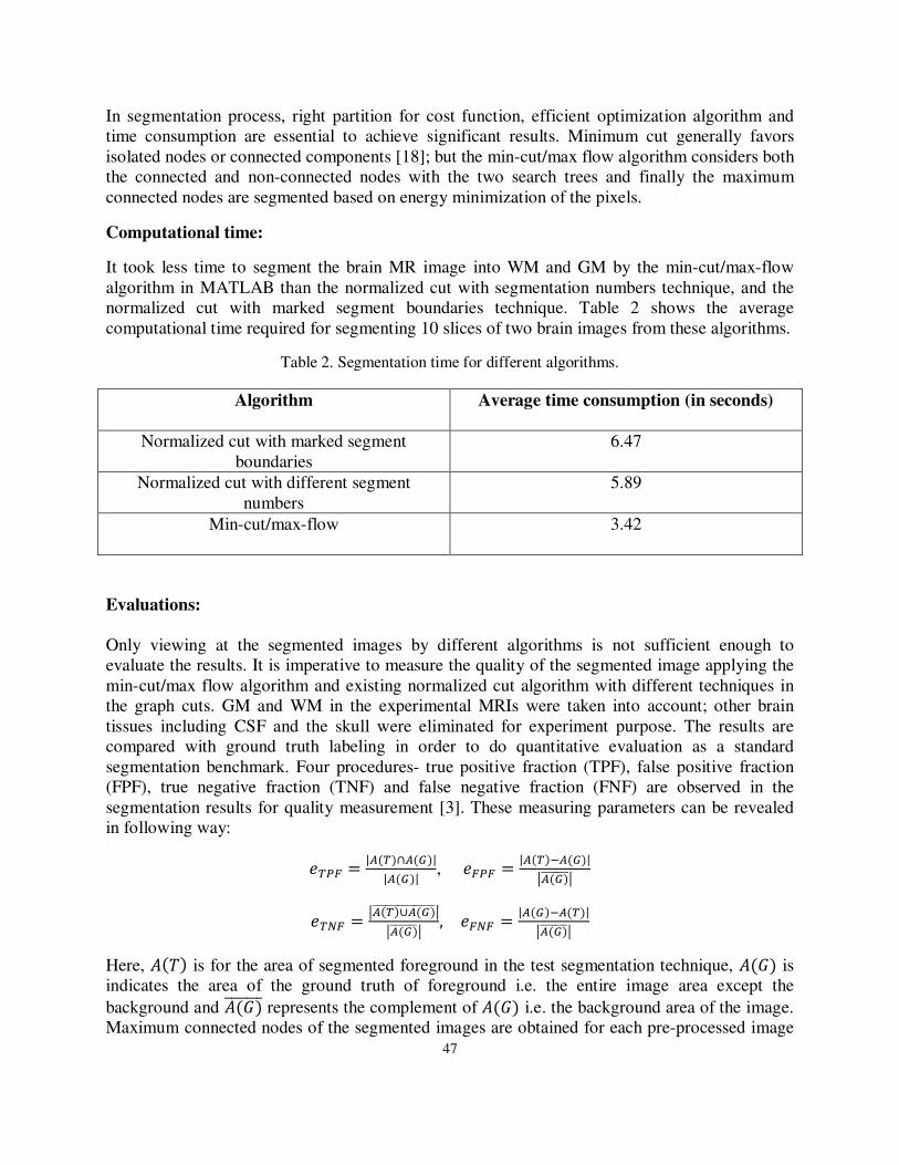
normalized cut with marked segment boundaries technique. Table 2 shows the average
computational time required for segmenting 10 slices of two brain images from these algorithms.
Table 2. Segmentation time for different algorithms.
Algorithm Average time consumption (in seconds)
Normalized cut with marked segment
boundaries
6.47
Normalized cut with different segment
numbers
5.89
Min-cut/max-flow 3.42
Evaluations:
Only viewing at the segmented images by different algorithms is not sufficient enough to
evaluate the results. It is imperative to measure the quality of the segmented image applying the
min-cut/max flow algorithm and existing normalized cut algorithm with different techniques in
the graph cuts. GM and WM in the experimental MRIs were taken into account; other brain
tissues including CSF and the skull were eliminated for experiment purpose. The results are
compared with ground truth labeling in order to do quantitative evaluation as a standard
segmentation benchmark. Four procedures- true positive fraction (TPF), false positive fraction
(FPF), true negative fraction (TNF) and false negative fraction (FNF) are observed in the
segmentation results for quality measurement [3]. These measuring parameters can be revealed
in following way:
-��� � |� ���� ��||� ��| , -��� � |� ���� ��|
E� �� E
-�}� � E� ��a� �� EE� �� E , -�}� � |� ���� ��|
E� �� E
Here, ¡ �� is for the area of segmented foreground in the test segmentation technique, ¡ 4� is
indicates the area of the ground truth of foreground i.e. the entire image area except the
background and ¡ 4� represents the complement of ¡ 4� i.e. the background area of the image.
Maximum connected nodes of the segmented images are obtained for each pre-processed image
48
for different threshold values. These values represent ¡ �� and ¡ 4� which are obtained by
MATLAB code and manual thresholding of T1 and T2. Three algorithms were tested over 10
slices of two brain MR images; the results are enlisted in Table 3.
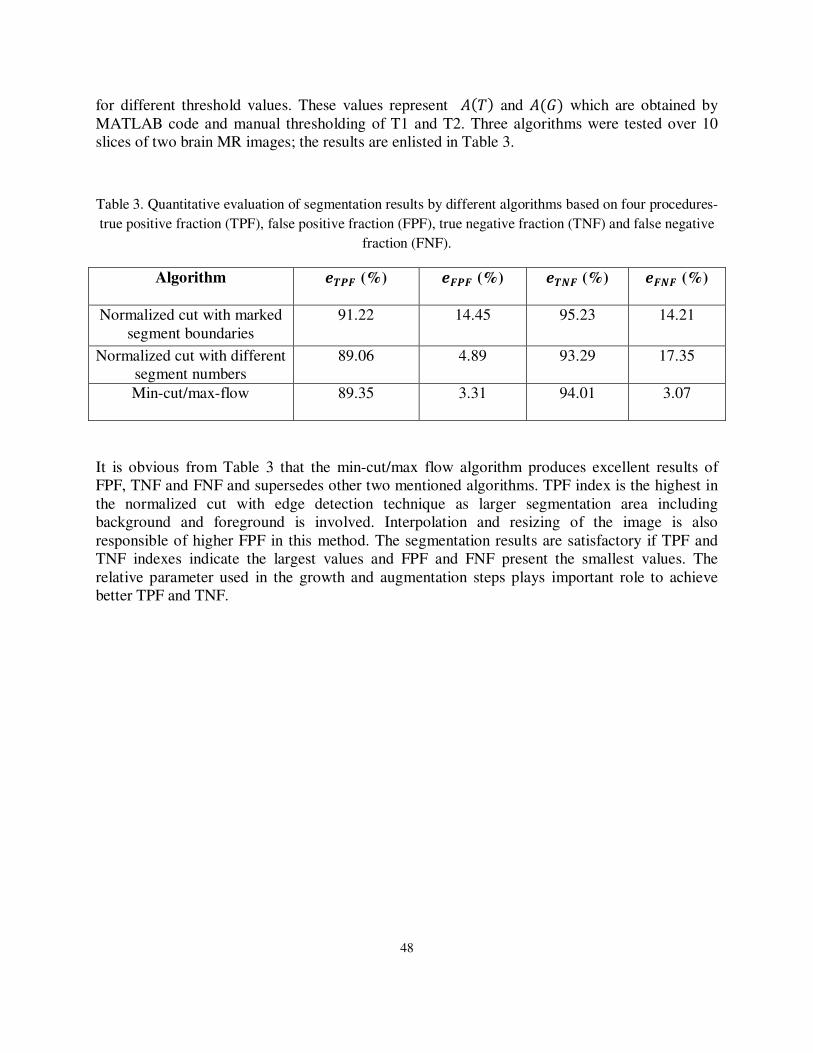
Table 3. Quantitative evaluation of segmentation results by different algorithms based on four procedures-
true positive fraction (TPF), false positive fraction (FPF), true negative fraction (TNF) and false negative
fraction (FNF).
Algorithm ¢£¤¥ (%) ¢¥¤¥ (%) ¢£¦¥ (%) ¢¥¦¥ (%)
Normalized cut with marked
segment boundaries
91.22 14.45 95.23 14.21
Normalized cut with different
segment numbers
89.06 4.89 93.29 17.35
Min-cut/max-flow 89.35 3.31 94.01 3.07
It is obvious from Table 3 that the min-cut/max flow algorithm produces excellent results of
FPF, TNF and FNF and supersedes other two mentioned algorithms. TPF index is the highest in
the normalized cut with edge detection technique as larger segmentation area including
background and foreground is involved. Interpolation and resizing of the image is also
responsible of higher FPF in this method. The segmentation results are satisfactory if TPF and
TNF indexes indicate the largest values and FPF and FNF present the smallest values. The
relative parameter used in the growth and augmentation steps plays important role to achieve
better TPF and TNF.
49
6. Discussions and Conclusions
6.1 Discussions
Three brain tissues- gray matter (GM), white matter (WM) and cerebrospinal fluid (CSF) are of
interest to be segmented by different algorithms. It has been found from the literature study that
the min-cut/max flow algorithm used in graph cuts is quite a new and potential method beside
the normalized cut and other algorithms. Image smoothness and energy minimization are basis of
this method. The purpose of this thesis was to conduct MRI brain image segmentation using two
algorithms namely the min-cut/max-flow algorithm and the normalized cuts for graph cuts.
The thesis research work comprises the detail study of this method to implement using an MRI
brain image. Pre-processing of the synthetic image, edges and boundaries detection after
convolution, histogram thresholding and finally segmentation of GM, WM and CSF are the
major steps in applying the min-cut/max flow algorithm. The segmentation of GM, WM and
CSF are also done by the normalized cut using marked segmentation boundaries and
segmentation number techniques. Existing simulations were used to apply these techniques in
brain MRI. Quantitative evaluation of these algorithms provides a comparison view in a standard
benchmark. 10 different slices of two brain images were pre-processed using approach A and B.
In approach A, pre-processing was conducted through MRIcroN software and the output was a
pre-processed image. A pre-processed image was generated using FSL software followed by
MRIcroN software in approach B. The brain image slices are without bones and the tissues are
segmented with less error in the pre-processing method B and therefore approach B was chosen
for test systems.
In the normalized cut algorithm the slices of brain image are interpolated and resized by 160x160
grey levels for both the marked segment boundaries and different segment numbers techniques.
Only WM tissue is segmented in the normalized cut with marked segment boundaries technique
while the regions are separated by the normalized pixel values of image data in the different
segment numbers technique. Therefore, it can be described that the marked segment boundaries
provide slightly better output than the different segment numbers technique.
The min-cut/max flow algorithm provided result that was slightly faster and with less error. WM,
GM and CSF are attempted to segment according to growth, augmentation and adaptation stages
to obtain minimum cut and maximum flow of images data. Two threshold values have been set
manually for each image that segregates the image pixel values in different regions based on
energy. The pre-processed and experimental images are not reshaped.
6.2 Conclusions
Analysis of the processed image data is one of the hot topics in imaging field where
segmentation plays vital role. Segmentation of medical images can be divided into two
classifications: a) manual, semi-automatic and automatic, b) pixel based local method and region
based global method [2]. Brain MR Image is a complex system to be segmented with efficient
method for having variable kind of tissues. Graph based approaches like graph cuts produce
50
significant output in the automatic and pixel based segmentation of brain MRI. Finding the
maximum flow from the source to the sink provides the solution of minimum cut in the graph
cuts method which is proved in the min-cut/max flow algorithm. Growth, augmentation and
adoption stages in this method with two search trees option for the connected nodes reveal the
segmentation performance to a new direction [6].
For brain MR image segmentation 10 different slices of two brain images have been tested in our
research for project simplicity and time constraints. The MR image segmentation experiments
were performed using both the normalized cut algorithm and min-cut/max-flow algorithm. The
preliminary test gives an impression that computational time and complexity are much less to
segment the brain MR image into WM, GM and CSF by the min-cut/max-flow algorithm
compared to the normalized cut algorithm. Furthermore, significant outputs for the segmentation
of WM, GM and CSF were produced by min-cut/max-flow algorithm. On the other hand
applying the normalized cut algorithm resulted in poor segmentation of WM, GM and CSF with
minimum quality. FSL and MRIcroN softwares were used for the pre-processing of brain MR
images. Extensive tests of various brain slices such as twenty brain images need to be conducted
along with other image analysis softwares in order to verify and improve the present results.
51
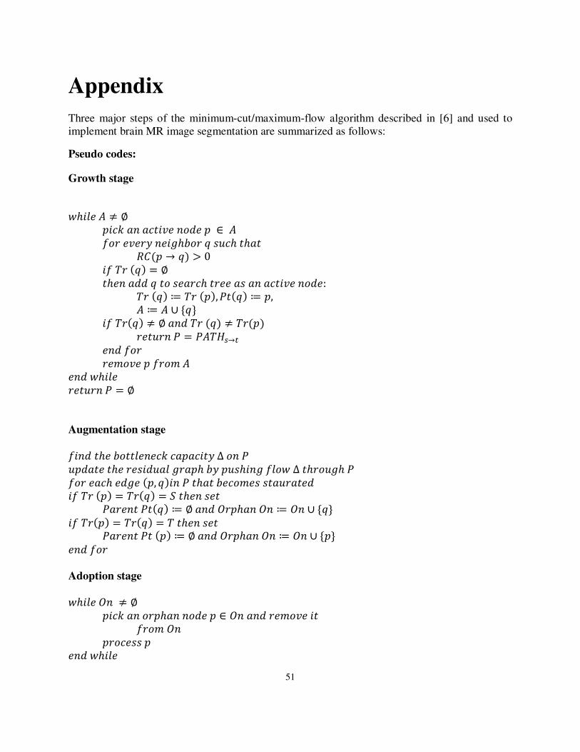
Appendix
Three major steps of the minimum-cut/maximum-flow algorithm described in [6] and used to
implement brain MR image segmentation are summarized as follows:
Pseudo codes:
Growth stage
w�$�- ¡ O h
.$�� �� ���$�- �p�- . b ¡ %pv -�-v! �-$��qpv X ���� ���� tY . � X� & 0
$% �v X� � h ��-� ��� X �p �-�v�� �v-- �� �� ���$�- �p�-: �v X� § �v .�,�� X� § ., ¡ § ¡ a BXC $% �v X� O h ��� �v X� O �v .�
v-��v� � � �¡� ]̈�\ -�� %pv v-p�- . %vp ¡ -�� w�$�- v-��v� � � h
Augmentation stage
%$�� ��- qp���-�-�� ��.��$�! ∆ p� � �.���- ��- v-�$���� �v�.� q! .���$�� %�pw ∆ ��vp��� � %pv -��� -��- ., X�$� � ���� q-�p-� ����v��-� $% �v .� � �v X� � � ��-� �-�
��v-�� �� X� § h ��� ev.��� e� § e� a BXC $% �v .� � �v X� � � ��-� �-� ��v-�� �� .� § h ��� ev.��� e� § e� a B.C -�� %pv
Adoption stage
w�$�- e� O h
.$�� �� pv.��� �p�- . b e� ��� v-p�- $� %vp e�
.vp�-�� . -�� w�$�-

52
The operation “.vp�-�� .” consists of the following steps: First, a new valid parent for . among
its neighbors is to be found. A valid parent X should satisfy �v X� � �v .�,tY X � .� & 0 and
the origin of X should be either source or sink. Note that the last condition is necessary because,
during the adoption stage, some of the nodes in the search trees � pv � may originate from
orphans.
If node . finds a new valid parent X then, we set �� .� � X. In this case . remains in its search
tree and the active (or passive) status of . remains unchanged. If . does not find a valid parent,
then . becomes a free node and the following operations are performed:
���� ��� �-$��qpv� X p% . �� �v X� � �v .�: $% tY X � .� & 0, ��� X �p ��- ���$�- �-� ¡ $% �� X� � ., ��� X �p ��- �-� p% pv.���� e� ��� �-� �� X� § h �v .� § h, ¡ § ¡ � B.C.
53
Bibliography
[1] R.C. Gonzalez, R.E. Woods and S.L.Eddins, “Digital image processing using MATLAB”,
Second edition, Gatesmark publishing, USA, 2009.
[2]Issac N. Bankman, “Handbook of medical image processing and analysis”, Second edition,
Academic press, USA, 2008.
[3] B. Peng, L. Zheng and J. Yang, “Iterated Graph Cuts for Image Segmentation”, Asian
Conference on Computer Vision (ACCV’09), Xi'an, China, September 23-27, 2009.
[4] Niessen et al. “Multiscale Segmentation of Volumetric MR Brain Images” published in
Signal processing for magnetic resonance imaging and spectroscopy by Marcel Dekker, Inc.
2002.
[5] M. Sonka, V. Hlavac and R. Boyle, “Image processing, analysis, and machine vision”, Third
edition, Thomson, USA, 2008.
[6] Boykov, Y., Kolmogorov, V.,” An experimental comparison of min-cut/max-flow algorithms
for energy minimization in vision”, IEEE Trans, Pattern Anal. Machine Intell., 26, 1124–1137,
2004.
[7] Geman, S., Geman, D., “Stochastic relaxation, gibbs distributions, and the Bayesian
restoration of images”, IEEE Trans, Pattern Anal. Machine Intell., 6, 721–741 classic, 1984.
[8] H. Ishikawa and D. Geiger, “ Segmentation by grouping junctions”, IEEE Conf. Computer
Vision and Pattern Recognition, pages 125–131, 1998.
[9] Y. Boykov and M. Jolly, “Interactive graph cuts for optimal boundary and region
segmentation of objects in n-d images”, Proceedings of ICCV, 2001.
[10] Boykov, Y., Veksler, O., Zabih, R., “Fast approximate energy minimization via graph cuts”,
IEEE Trans. Pattern Anal. Machine Intell., 23(11), 1222–1239, 2001.
[11] Y. Boykov, O. Veksler, and R. Zabih, “ Markov random fields with efficient
approximation”, IEEE Conference on Computer Vision and Pattern Recognition, pages 648–655,
1998.
[12] Greig, D., Porteous, B.T., Seheult, A.H., “ Exact maximum a posteriori estimation for
binary images”, J. R. Stat. Soc., B 2, 271–279, 1989.
[13] V. Kwatra, A. Schdl, I. Essa, G. Turk, and A. Bobick, “Graphcut textures: Image and video
syntesis using graph cuts”, ACM Transactions Graphics, Proc. SIGGRAPH, July 2003.
[14] H. Ishikawa and D. Geiger, ”Oclusions, discontinuities, and epipolar lines in stereo”, Fifth
European Conference on Computer Vision, (ECCV’98), Freiburg, Germany, 2-6 June 1998.
[15] S. Roy and I. Cox, ”A maximum-flow formulation of the n-camera stereo correspondence
problem”, Int. Conf. On Computer Vision, ICCV’98, Bombay, India, 1998.
[16] S. Roy and M.-A. Drouin, “Non-uniform pyramid stereo for large images”, IEEE Workshop
on Stereo and Multi-Baseline Vision, Kauai, Hawaii, 2001.
[17] Kolmogorov, V., Zabih, R., “What energy functions can be minimized via graph cuts?”,
IEEE Trans. Pattern Anal. Machine Intell. 26(2), 147–159, 2004.
[18] J. Shi and J. Malik, “Normalized cuts and image segmentation”, IEEE Conference on
Computer Vision and Pattern Recognition, pages 731–737, 1997.
[19] L.P. Clarke et al. “MRI Segmentation – Methods and Applications”, Review, Elsevier
Science Ltd, Magnetic Resonance Imaging, Vol. 13, No. 3, pp. 343-368, 1995.

54
[20] L. R. Foulds, “Graph Theory Applications”, Springer-Verlag New York Inc., 247-248,
1992.
[21] Chris Rorden, “MRIcroN free software”, Version 15, October 2008, webpage:
www.cabiatl.com/mricro, www.nitrc.org/projects/mricron, accessed on 25 SEPT 2010.
[22] “FMRIB Software Library (FSL)”, Version 4.1, August 2008, webpage:
www.fmrib.ox.ac.uk/fsl, http://www.fmrib.ox.ac.uk/fsl/fsl/downloading.html, accessed on 25
SEPT 2010.
[23] S.M. Smith et al., “Advances in functional and structural MR image analysis and
implementation as FSL”, NeuroImage, 23(S1):208-219, 2004.
[24] Zhuang Song, Nicholas Tustison, Brian Avants, and James C. Gee, “Integrated Graph Cuts
for Brain MRI Segmentation”, MICCAI 2006, LNCS 4191, pp. 831–838, 2006.
[25] J. Shi and J. Malik, “Ncut and image segmentation”, IEEE Trans. PAMI, 22(8):888–905,
August 2000.
List of Figures
Figure 1. Bimodal histogram of an image f(x, y) with selected threshold T. .................................9
Figure 2. Example of graph construction from a 3x3 image and 2D segmentation (a) Image with
seeds such as background, B and object, O (b) Graph construction for two kinds of vertices,
edges and pixels i, j, i, j,k, l, m b n (c) Graph cuts segmentation (d) Segmentation results.. .. 15
Figure 3. Graph formation from an image, I = {pixels} having source, sink and edge connection
nodes......................................................................................................................................... 17
Figure 4. Graph formation, � � B�, �C with three tissues-GM, WM and CSF for brain MRI
segmentation. ............................................................................................................................ 18
Figure 5. Example of the min-cut/max-flow algorithm in graph cuts segmentation .................... 18
Figure 6. An example of minimum cut that provides bad partition ............................................. 19
Figure 7. Block diagram of MRI brain image segmentation based on min-cut/max-flow
algorithm................................................................................................................................... 21
Figure 8. Block diagram of two different pre-processing approaches for MRI brain image
analysis (a) pre-processing approach A: extracted using MRIcroN software (source: NITRC- The
source for neuroimaging tools and resources) (b) pre-processing approach B: extracted using
FSL software (source: FMRIB software library) followed by MRIcroN software. ..................... 22
Figure 9. Pre-processing approach A using MRIcroN software for displaying the selected slice of
brain image. .............................................................................................................................. 23
Figure 10. Pre-processing approach B using FSL software followed by MRIcroN software for
displaying the selected slice of brain image. .............................................................................. 24
Figure 11. Pre-processed (using approach B) MRI image: Gray matter (GM), white matter (WM)
and Cerebrospinal Fluid (CSF). ................................................................................................. 25
Figure 12. Left: Edges detection, right: boundaries detection of the pre-processed (using
approach B) MRI image. ........................................................................................................... 26
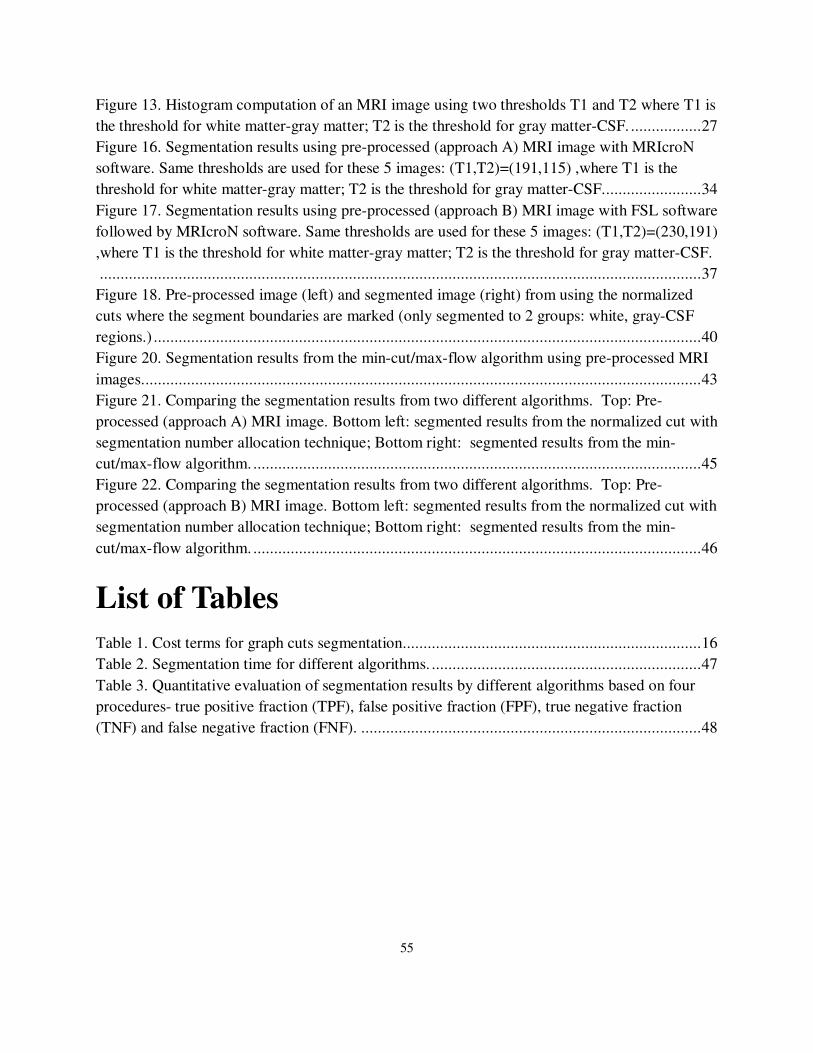
55
Figure 13. Histogram computation of an MRI image using two thresholds T1 and T2 where T1 is
the threshold for white matter-gray matter; T2 is the threshold for gray matter-CSF. ................. 27
Figure 16. Segmentation results using pre-processed (approach A) MRI image with MRIcroN
software. Same thresholds are used for these 5 images: (T1,T2)=(191,115) ,where T1 is the
threshold for white matter-gray matter; T2 is the threshold for gray matter-CSF. ....................... 34
Figure 17. Segmentation results using pre-processed (approach B) MRI image with FSL software
followed by MRIcroN software. Same thresholds are used for these 5 images: (T1,T2)=(230,191)
,where T1 is the threshold for white matter-gray matter; T2 is the threshold for gray matter-CSF.
................................................................................................................................................. 37
Figure 18. Pre-processed image (left) and segmented image (right) from using the normalized
cuts where the segment boundaries are marked (only segmented to 2 groups: white, gray-CSF
regions.) .................................................................................................................................... 40
Figure 20. Segmentation results from the min-cut/max-flow algorithm using pre-processed MRI
images. ...................................................................................................................................... 43
Figure 21. Comparing the segmentation results from two different algorithms. Top: Pre-
processed (approach A) MRI image. Bottom left: segmented results from the normalized cut with
segmentation number allocation technique; Bottom right: segmented results from the min-
cut/max-flow algorithm. ............................................................................................................ 45
Figure 22. Comparing the segmentation results from two different algorithms. Top: Pre-
processed (approach B) MRI image. Bottom left: segmented results from the normalized cut with
segmentation number allocation technique; Bottom right: segmented results from the min-
cut/max-flow algorithm. ............................................................................................................ 46
List of Tables
Table 1. Cost terms for graph cuts segmentation........................................................................ 16
Table 2. Segmentation time for different algorithms. ................................................................. 47
Table 3. Quantitative evaluation of segmentation results by different algorithms based on four
procedures- true positive fraction (TPF), false positive fraction (FPF), true negative fraction
(TNF) and false negative fraction (FNF). .................................................................................. 48