Monetary Reference Points of Managers

March 2012

VERY PRELIMINARY VERSION

PLEASE DO NOT QUOTE

Authors:

Christian GRUND, University of Duisburg-Essen, Mercator School of Management, Lothar-

strasse 65, 47057 Duisburg, Germany, E-Mail: christian.grund@uni-due.de, Tel: ++49 203

379 4369

Johannes MARTIN, University of Duisburg-Essen, Mercator School of Management, Lothar-

strasse 65, 47057 Duisburg, Germany, E-Mail: johannes.martin@uni-due.de, Tel: ++49 203

379 4312

Monetary Reference Points of Managers

Abstract

We assemble two reference point based concepts of utility in our empirical study: the own

status quo and social comparisons. We explore the relative relevance of these concepts for

total compensation as well as for different parts of the compensation package of managers.

Making use of a unique panel data set of managers of the German chemical sector, we find

that social comparisons of compensation indeed affect reported job satisfaction. Managers

compare their total compensation (and fixed salary) with others in the chemical sector and

report lower satisfaction scores when they earn less than similar managers. There is less evi-

dence for the relevance of status quo preferences.

JEL-Codes: M5, D03, J30, J28

Keywords: Compensation, Job satisfaction, Reference points, Social comparisons, Status quo

preferences

1

1 Introduction

It is now more and more established in (behavioral) personnel economics that in many situa-

tions individuals do not care exclusively for their own outcome, but also take certain refer-

ence points into account. These possible reference points include the own hitherto status quo

or social comparisons with peers.

Income comparisons among employees played for a long time a minor role in the economic

literature (see Drakopoulos (2011) for an overview over the history of earnings comparisons

in economics). However, first theoretical foundations of the own hitherto status quo as refer-

ence point trace back to the contributions of Duesenberry (1949) and Markowitz (1952). They

focused especially on consumption decisions. Prospect Theory (Kahneman & Tversky 1979,

Tversky & Kahneman 1991) enhanced these approaches: Individuals evaluate a specific

amount of money or other goods not only with respect to its absolute value, but also relative

to a certain reference point. In this context, it is often assumed that negative deviations from

this reference point lead to a higher increment of disutility than positive deviations in the

same size lead to an increment of utility (loss aversion). Easterlin (1995, 2001) explains these

status quo preferences with increased aspiration levels over time.

In the context of social comparisons, first theoretical considerations are the Social Compari-

son Theory of Festinger (1954) and the Equity Theory of Adams (1963). It is argued that in-

dividuals compare themselves with similar persons (neighbours or colleagues, for instance).

These comparisons may then affect perceived utility and behaviour. Akerlof (1984) and Aker-

lof & Yellen (1990) apply these arguments to considerations in the economics literature and

argue that effort choice in employment relationships depend on fairness considerations. Based

on experimental evidence, Fehr & Schmidt (1999) as well as Bolton & Ockenfels (2000) offer

specific utility functions, which take individuals’ inequality aversion into account. In contrast,

2

Frank (1985) argues that individuals have certain status preferences perceiving a benefit from

a higher status (with respect to wages, for instance) than comparable persons. Besides,

Hirschman & Rothschild (1973) describes a tunnel effect, i.e. higher wages of reference per-

sons could reflect a signal for future own wages.

If the two types of reference points matter, individuals acting in a role as an employee may

then take their own wage of the previous period or the wage of other employees into consid-

eration in order to evaluate their own current income.

Previous empirical contributions either focus on the status quo or social comparisons of indi-

viduals. Some papers examine the impact on human behaviour in terms of effort, performance

or labour supply (e.g. Camerer et al. 1997, Farber 2005 and 2008, Mas 2006, Mas & Moretti

2009, Ockenfels et al. 2010). Other papers analyse more directly, whether monetary reference

points affect subjective well-being or job satisfaction. Hereby, one strand of the literature

gears to the previous status quo as possible reference point. Clark (1999) analyses employee

data of two waves of the British Household Panel Survey (BHPS). In his cross-sectional in-

vestigation, he finds a strong positive correlation between the change in hourly pay and job

satisfaction. Grund & Sliwka (2007) confirm this finding with panel data of 19 waves of the

German Socio-Economic Panel (GSOEP). The results hold true for highly skilled white-collar

workers in particular.

Other contributions analyse the relevance of social comparisons, i.e. the comparison with

peers. The empirical strategy varies across studies. The seminal paper of Clark & Oswald

(1996) makes use of the 1991 wave of the BHPS. In order to calculate the reference wage,

they estimate a Mincer-type wage regression with a bunch of wage determinants and predict

the expected wage for all individuals. Hence, the reference point indicates the wage an em-

ployee with given individual and firm characteristics can expect in the labor market on aver-

3

age. They find a significantly negative correlation between job satisfaction and this reference

point, given a certain own wage level. Ferrer-i-Carbonell (2005) defines the reference point as

the average income of individuals living in the same region with the same education and the

same age. She uses panel data of the German Socio Economic Panel (GSOEP) shows that the

more individuals earn in comparison to their reference groups, the more satisfied they are. In

addition, this effect is asymmetric, which means that individuals with an income below the

reference point are more dissatisfied than individuals with an income above the reference

point in the same amount are satisfied. Clark et al. (2009a) stick to income comparisons with

the nearby neighbourhood. Using administrative data matched with eight waves of the Danish

European Community Household Panel (ECHP), they find a positive effect of the richness of

the neighbourhood on the economic satisfaction of individuals. However, the relative position

within the neighbourhood is important too: The higher individuals are located in the income

distribution, the more satisfied they are. FritzRoy et al. (2011) compare the relevance of social

comparisons in Germany and in Great Britain using panel data of the GSOEP and the BHPS.

They define the reference group as individuals with same age, education, gender and living in

the same region. Interestingly, they find an age-dependent impact of the reference income for

Germany: Whereas life satisfaction is negatively correlated with the average income of the

comparison group for those over 45, this correlation is positive for those under 45. They in-

terpret this finding as a confirmation of Hirschman´s tunnel effect that individuals interpret

higher wages of peers as signals for possible own wages in the future. For Great Britain, the

satisfaction effect of the reference income is negative for all age groups.

Some few studies analyse social comparisons on the level of firms. Brown et al. (2008) use

data of the British Workplace Employee Relations Survey of 1998 and focus on employees.

They operationalize monetary reference points by computing the individual wage rank within

the firm. They find a highly significant and positive correlation of the wage rank with differ-

4

ent measures of satisfaction. Moreover, the effect of the relative income position seems to be

stronger as of the absolute pay itself. Clark et al. (2009b) match (as in Clark et. al (2009a),

too) waves of the Danish ECHP with administrative data. The results show that own earnings

matter for job satisfaction, but also average earnings within the establishment do: the higher

the mean pay in their firm is, the more satisfied workers are. The authors argue in this context

that the definition of the reference group is very important for the direction of the effect.

When the wages of other could be my own future earnings (as with respect to wages of co-

workers), than the effect is rather positive – wages exert a signal. However, when comparison

earnings are not reachable for me, I interpret those as an indication of a higher social status of

others and hence the effect should be negative. Card et al. (2010) conduct a field experiment

with about 6,000 employees at the University of California. Within this experiment, a treat-

ment group of employees gets information about a new website where wages of University

employees are listed. Other employees in the control group are not informed. They find a

clear result: The information of the treatment group exerts a negative effect on the satisfaction

of individuals who are paid the median wage of their unit and occupation, i.e. workers with

comparable tasks. There is no effect, however, for people who are paid over the median. One

conclusion by the authors is that it could be better for employers to keep secrecy regarding the

payments of their employees. The possibly closest contribution with respect to our data is

Ockenfels et al. (2010). They compare executives of one multinational firm in two plants in

Germany and the U.S. As they have information about the achievement of individual targets

of the managers, they define the reference point as a bonus percentage of 100 percent. The

bonus payment depends on how good managers have fulfilled their targets. Thereby, a value

of 100 percent means that the manager fully meets the expectations of the supervisor. Fur-

thermore, the bonus budget of supervisors is restricted which implies that they have to cut the

payment of one or more managers if they want to pay other managers a higher bonus. In con-

5

sequence, bonus percentages under the reference point could be understood as negative refer-

ence point violations. In the German plant, job satisfaction of managers is significantly re-

duced if they fall below the reference point, but there is no effect on satisfaction of managers

with bonus percentages over 100 percent. In the U.S., there is no significant effect. The au-

thors explain this finding with the communication policy of the firm. American managers get

no information about their bonus percentages, whereas German managers are fully informed.

Hence, the results of this study suggest too that firms could be better off when keeping secre-

cy about earnings.

In conclusion, the results imply that individuals perceive a lower utility in most cases when

their wage is below a certain social reference wage. But the effects of reference points depend

on the selection of the reference person or group. However, all of these studies analyse one

possible reference point (either the previous status quo or social comparisons) and one meas-

ure of monetary outcome (fixed salaries, bonus, total compensation) only. It is therefore not

possible to evaluate the relative relevance of the two concepts up to now. In contrast to pre-

vious work that focused on one possible reference point, we assemble both concepts and ex-

plore their relative relevance. We address the following questions in particular:

(1) To what extent is job satisfaction affected by deviations from the hitherto compensation

(status quo) and by differences from others´ compensation (social comparison)?

(2) Are there differences between wage components?

(3) Are there differences between comparisons on the firm level and on the industry level?

We make use of a unique panel dataset with rich information on income components, work

situation and socio-demographics of managers of the German chemical sector. We measure

the perceived utility from a job with the reported job satisfaction. In contrast to previous

6

work, we examine not only one but both of the two types of reference points. First, we have

longitudinal information about the manager´s income so that we are able to investigate the

relevance of possible deviations of the hitherto status quo. Second, the data includes infor-

mation about the firm and the hierarchical level of the managers and, thus, allows us to define

certain reference groups that managers could compare their income with. We hereby distin-

guish between the market and the firm level. Ex ante it is not clear, whether employees com-

pare themselves with colleagues of the same firm or also with employees in similar jobs of

other firms. Evidence may differ across wage components, too. We offer a separate examina-

tion for total compensation as well as for fixed salaries and bonus payments..

The remainder of the paper is structured as follows: In chapter 2, we describe our data and our

variables. Afterwards, we present our empirical strategy and our results in chapter 3. Finally,

chapter 4 discusses the results and concludes.

2 Data and Variables

We can make use of a unique panel data set of highly qualified professionals and executives

of the German chemical industry. We conduct a corresponding annual salary survey in col-

laboration with the German association of executive staff of the chemical industry (Verband

angestellter Akademiker und leitender Angestellter der Chemischen Industrie e.V. (VAA)).

According to VAA, our sample is representative for the respective employees of the chemical

sector. Individuals are asked about their current job next to some demographics and their pre-

vious occupational career. In particular, we have detailed information on all components of

their compensation such as fixed salaries and bonus payments as well as other integral parts

7

such as exercised stock options, inventors’ gratuities or jubilee payments. Grund & Kräkel

(forthcoming) provide some more information of the data.

We can make use of the first three waves of this survey of the years 2009 to 2011. Compensa-

tion data are collected in retrospect so that the data cover the period from 2008 to 2010. We

restrict our sample to fulltime employees in West German plants who have a university de-

gree in natural science or engineering. The VAA negotiates an annual collective agreement

with the employers concerning minimum wage levels and working conditions. This contract

is only valid for such managers with a university degree in natural sciences and engineering,

who account for 0.88 of our sample. Since we also want to address the role of certain wage

components, fixed salary and bonus payments in particular, only employees with a bonus con-

tract are considered. Due to these restrictions, we have got a sample size of 11.077 observa-

tions over the three year period. Each year we have information of about 3.700 managers. We

can follow individuals over time and have got an unbalanced panel.

We explore the role of compensation for the perceived utility from work. We therefore use

reported job satisfaction of managers as its proxy (see already Freeman (1978) for reasoning

that job satisfaction is an economically highly relevant variable). General job satisfaction is

surveyed with the question “How satisfied are you with your job?” on an 11-digit scale from 0

(totally unhappy) to 10 (totally happy). The average reported job satisfaction is 6.85 with the

median and mode at 8 (Table 1 and Figure 1 in the Appendix). The distribution does not differ

very much to the whole group of employees in Germany (see Grund & Sliwka 2007) for cor-

responding evidence).

We have detailed information on individuals’ compensation. Bonus payments are prevalent

for managers in the sector. Some employees also report other additional monetary parts of

compensation such as exercised stock (options) or gratuities for inventions next to their fixed

8

salary. The average annual total compensation of the managers in our sample amounts to al-

most € 120.000. The main part (80 %) of compensation is assigned to fixed salaries and 15 %

account for bonus payments (see Table 1). The observation period covers an economically

successful year of the German chemical sector (2008) and the subsequent economic crisis.

The fraction of bonus payments on total compensation in our sample decreases only slightly

from 0.17 in the year 2008 to 0.14 in 2010, though.

We explore the role of monetary reference points next to the own compensation of the current

period. We use reported compensation of the previous year as our measure for the hitherto

status quo. Doing this, we lose a considerable number of observations (in particular those of

the first wave of our panel). Additionally we compute social comparison wages by estimating

Mincer type wage regressions and using the results for calculating predicted wages for indi-

viduals. A manager with certain characteristics – we control for the level of the hierarchy,

work experience and firm size – earns on average the predicted wage. We compute these

comparison wages at two levels of the analysis. First, we refer to the market level and use all

observations of our sample. Second, we run the wage regressions on the firm level arguing

that colleagues may be the relevant reference group. Doing this, we can only make use of

firms with a considerable number of observations. We restrict our analysis to ten large firms.

Some more detailed information on these reference wages are given at the corresponding sub-

sections of the empirical investigation below.

We make use of a bunch of control variables in our regression analysis on job satisfaction of

the following section. These control variables include socio-demographic characteristics such

as sex, being in a relationship, having children and experience as well as job and firm level

factors, which include the distance from home to the workplace (in km), tenure (in years),

9

firm size (8 dummies) and level of the hierarchy (4 dummies, with level 1 representing top

management positions).

Table 1 about here

3 Empirical Strategy and Results

3.1 Status Quo Preferences

We argued above that the salary or certain wage components of the previous year may act as

reference points in the sense of a hitherto status quo. We will explore the role of fixed salary

and bonus payments next to total monetary compensation. Then the actual salary and also

deviations from the previous year may have an effect on job satisfaction (see Clark & Oswald

1996 as well as Grund & Sliwka 2007 for previous evidence).

Individual reported job satisfaction in the actual year acts as the dependent variable. Because

of its ordinale scale, ordinal probit estimates would be one possibility. We stick to linear re-

gressions so that the effect size of the results can be interpreted more easily. Job satisfaction is

measured on an 11-digit scale so that there are not to few different values. We apply random

effects models since we have only three years and an overlap of individuals from year to year

of about 0.6. The qualitative results do not differ between linear and ordered probit model

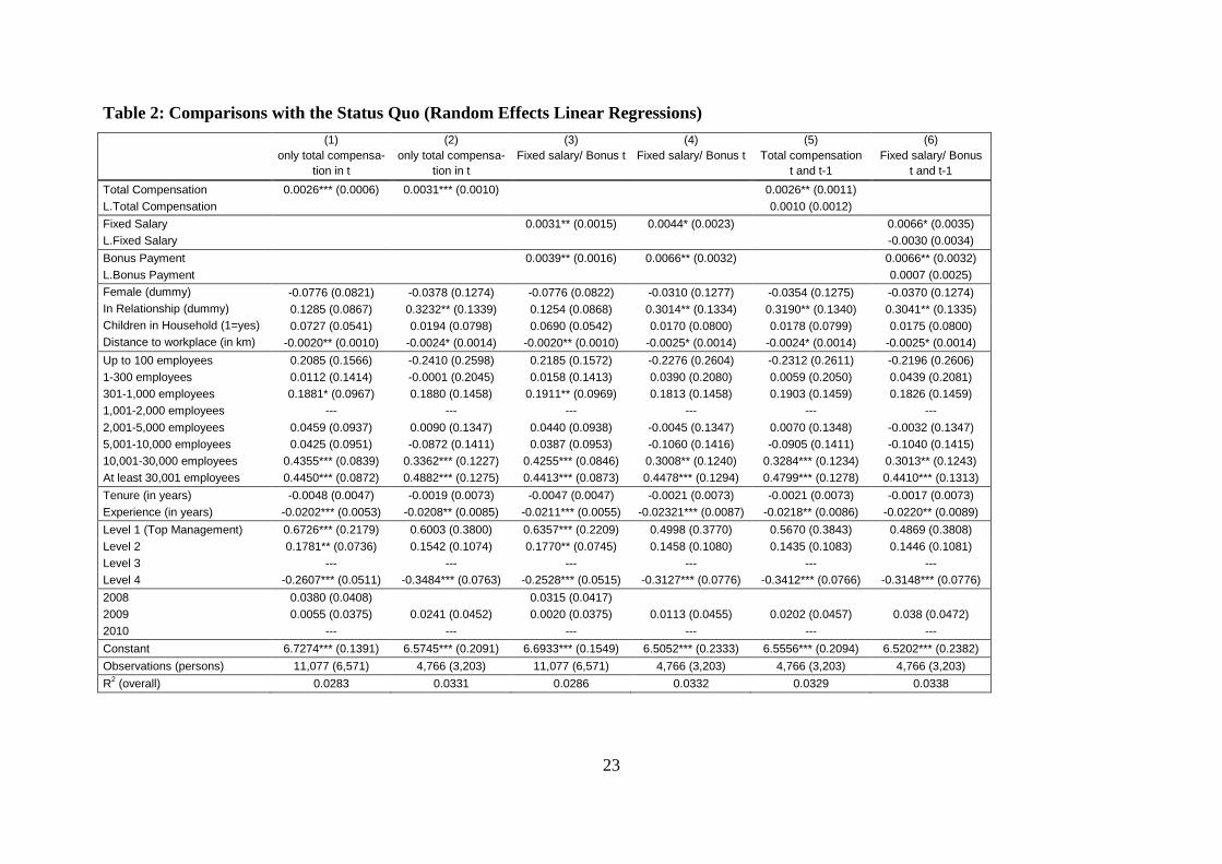
estimates. The wage of the current year (t) and the previous year (t-1) act as the decisive inde-

pendent variables. In a first step, we only insert the wage of the current period (model (1) of

Table 2). Indeed, we find a significant relation between the wage and job satisfaction. Be-

cause of the structure of our data, we lose a considerable number of observations by including

10

the wage of the previous period. All observations of the first wave are dropped in particular.

Model (2) of Table 2 is just a re-estimate of model (1) with the observations for which we

have information for the wage of previous period. The sample size drops from about 11.000

to about 5.000. The results are robust with respect to this restriction. Models (3) and (4) show

corresponding specifications with the fixed salary and the bonus payment instead of total

compensation. Both are positively associated with job satisfaction. The size of the coefficients

does not differ dramatically.

The results for the other independent (control) variables show that job satisfaction is positive-

ly related to firm size, being in a relationship and the level of the hierarchy, while it is nega-

tively associated to the distance of the home to the workplace and experience.

Including the wage of the previous year, the following estimation applies:

Job satisfactiont = α + β · waget + γ · waget−1 + δ'X + ε. (1)

The vector of the other independent variables is characterized by X. A simple transformation

shows that the effect of wage increases is directly captured with this approach:

JSt = α + (β + γ) · waget – γ · (waget – waget−1) + δ'X + ε. (2)

Hence, evidence for status quo preferences would be revealed by a negative and significant

estimate of γ. The results of estimations of equation (1) and (2) are equivalent in terms of the

estimated coefficients α, β, γ, and δ. Model (5) shows that we do not find support status quo

preferences concerning total compensation. The coefficient of the compensation of the previ-

ous year is not significant and its sign is positive instead of negative as expected. We do not

find evidence with respect to changes in fixed salaries or bonus payments, either (model 6).

11

Table 2 about here

This approach is based on the assumption that the satisfaction effect of the previous status quo

is equal for all managers, no matter whether they earn more or less than before. However,

under the assumption of loss aversion, managers are supposed to evaluate wage decreases

stronger than wage increases. Figure 2 illustrates this idea with two different curves. The

dashed line represents the effect on job satisfaction in the absence of loss aversion which is

the result of an estimation of equation (2). In contrast, the continuous curve with the kink in

the origin stands for the situation under the assumption of loss aversion.

Figure 2 about here

To test this approach econometrically, we extend equation (2):

JSt = α + β · waget + γ · (waget – waget−1) + δ · (waget – waget−1) · Decrease + η'X + ε. (3)

Decrease represents a dummy which adopts the value 1 if the manager earns less than the

year before. The evidence of loss aversion would be revealed by positive and significant coef-

ficient δ, which would indicate the steeper slope of the curve below the origin in Figure 2.

Note that, due to the interaction term, the coefficients of this equation are no more identical to

the coefficients of equations (1) and (2). Table 3 shows the results for total compensation

12

(model 1) and fixed salaries and bonus payments (model 2). However, we do not find evi-

dence for loss aversion, too.1

Table 3 about here

In the following subsection, we explore whether there is more evidence of the role of social

comparisons for utility of work reported by job satisfaction.

3.2 Social Comparisons and Job Satisfaction

As mentioned above, we investigate the relevance of social comparisons on two different lev-

els. On the one hand, managers may compare themselves with the whole labor market of the

chemical industry. Wages within the sector are transparent to a certain extent, as the VAA

publish an annual brochure including a bunch of analyses regarding the earnings of their

members (based on the same dataset used in this paper). We think that managers have some

possibilities to compare their wages with those of others. We operationalize the reference

wage by the predicted wage managers would earn on average with their characteristics on the

market. We estimate Mincer-type wage regressions for total compensation, fixed salary and

bonus payments. As wages within the chemical industry differ considerably between the three

years, we estimate separate cross-sectional OLS regressions by year. Within the estimation

equation, we control for firm size, work experience and hierarchical level, as these are the

1 However, there is a slightly significant and negative effect of the interaction term with respect to fixed salaries.

In our data, only 7.5 percent of all managers suffer decreases in their fixed salaries from one year to another.

These are mostly due to job or firm changes. Hence, the positive effect on job satisfaction is not supposed to be

due to wage cuts, but rather because of positive developments in the work environment.

13

most important determinants of wages within the chemical industry.2 In consequence, the pre-

dicted wage reflects the wages executives would earn on average with their individual firm

size, work experience and hierarchical level in a given year.

Besides these social comparisons with other managers in the market, managers may compare

their income with the income of their intra-firm colleagues. Our operationalization of the cor-

responding reference wage is similar as we also predict wages by running Mincer-type wage

regressions. However, we thereby include only observations of the particular firm. Analo-

gously, we run separate cross-sectional regressions for each of the three years. We control for

work experience and hierarchical level. Hence, the predicted wage in this case reflects the

income managers earn on average with their given work experience on their given level in

their firm. Doing so, we can only focus on some bigger firms with sufficient observations in

the single years so that we focus on the ten biggest firms.

We then include the predict wage in our estimation equation:

JSt = α + β · waget + γ · wageref, t + δ'X + ε. (4)

A simple transformation leads to a similar equation as in the case of status quo preferences:

JSt = α + (β + γ) · waget – γ · (waget – wageref, t) + δ'X + ε. (5)

Hence, γ indicates the relevance of social comparisons. Given a significant influence, a nega-

tive sign would indicate preferences for an own wage that is higher than that of the peers. Es-

timations of the models (4) and (5) would lead to equivalent results with respect to the esti-

mated coefficients.

2 The Adjusted R

2 of these OLS estimations reaches over 60 percent.

14

In all other respects, the estimations are identical to those presented in section 3.1 for status

quo preferences. The results are shown in Table 4. In model (1) we include total compensa-

tion and the total reference compensation on the market level. The highly significant and neg-

ative sign indicates that the more managers earn relative to managers on the market, the high-

er is their job satisfaction. The effect of the own total compensation is highly significant too,

but much smaller than that of the reference wage. Model (2) reveals the results for both fixed

salary and bonus payments. The picture for fixed salary is similar to total compensation with a

positive influence of the own wage and a negative effect of the reference wage. Regarding

bonus payments, however, we get a positive and highly significant effect of the own bonus,

but no significant influence of the reference bonus. The sign is even positive.

In model (3) and (4), we focus on intra-firm social comparisons. As mentioned above, we

thereby concentrate on the ten biggest firms. However, we don´t get many significant results.

Only the own fixed salary exert a significant influence on job satisfaction.

Table 4 about here

Similar to the situation of status quo preferences and loss aversion, there are also some hints

that managers who earn less than their peer group are more influenced by the reference in-

come than managers with an income above the reference wage are. One explanation could be

the higher relevance of negative than positive inequality aversion (Fehr & Schmidt 1999). We

define this case as social loss aversion. To test whether there is evidence for this assumption,

we extend model 5:

JSt = α + β · waget + γ · (waget – wageref,t) + δ · (waget – wageref, t) · Below + η'X + ε. (6)

15

Below is a dummy adopting the value 1 when the manager earns less than the respective ref-

erence income. Hence, a positive and significant coefficient δ would prove that the effect of

the reference income is especially strong for managers with wage < wageref. Table 5 shows

our results. There is evidence of social loss aversion regarding total compensation on both

market and firm level as well as regarding bonus payments on the market level.

Table 5 about here

4 Conclusion

In the traditional view of economics, individuals are egoistic and exclusively care of their

own income. However, several approaches in the field of behavioral economics suggest that

workers also take certain monetary reference points into account when evaluating their in-

come situation. Using a unique dataset of executives in the German chemical sector, we ex-

plore the relevance of two different possible reference points: the own wage from one year

before (status quo preferences) and the wages of comparable managers (social comparisons).

Job satisfaction (as a proxy for utility from work) is significantly correlated with the absolute

value of total compensation, fixed salaries, and bonus payments. Though, we find no evidence

for status quo preferences, i.e. wage payments from previous years seem to be not relevant for

managers. However, we find highly significant effects with respect to social comparisons with

other managers in the labor market, at least for total compensation and fixed salaries. The

partial effects are even higher than those of the own wages. This effect is even stronger when

executives earn less than the reference income. When we investigate social comparisons with

co-workers in the same firm, however, we find less evidence associations to job satisfaction.

16

The analysis of subgroups with respect to sex is left for future research. Furthermore, instead

of absolute wage differences, one may assess the impact of relative wage differences. Instead

of estimated reference wages, ranks and percentiles may also be useful measures for reference

incomes (see Brown et al. 2008). Finally, the synthesis of both reference point concepts is an

exciting task for future research: It may well the case that managers compare their own wage

increases to the wage increases of their co-workers in particular.

17

References

Adams, J. S. (1963): Toward an Understanding of Inequity. In: Journal of Abnormal and

Social Psychology (67), 422-436.

Akerlof, G. A. (1984): Gift Exchange and Efficiency-Wage Theory: Four Views. In:

American Economic Review (74), 79-83.

Akerlof, G. A.; Yellen, J. L. (1990): The Fair Wage-Effort Hypothesis and Unemployment.

In: Quarterly Journal of Economics (105), 255-283.

Bolton G.E.; Ockenfels A. (2000): A Theory of Equity, Reciprocity, and Competition. In.

American Economic Review 100:166-193.

Brown, G. D. A.; Gardner, J.; Oswald, A. J.; Qian, J. (2008): Does wage Rank Affect

Employees Well-being? In: Industrial Relations 47, 355-389.

Camerer, C. F., Babcock, L., Loewenstein, G., Thaler, R. (1997): Labor Supply of New

York City Cab Drivers: One Day at a Time. In: Quarterly Journal of Economics, 111,

408-41.

Card, D., Mas, A., Moretti, E., Saez, E. (2010): Inequality at Work: The Effect of Peer

Salaries on Job Satisfaction. NBER Working Paper 16396.

Clark, A. E. (1999): Are Wages Habit-Forming? Evidence from Micro Data. In: Journal of

Economic Behavior & Organization, 39, 179–200.

Clark, A. E., Kristensen, N., Westergård-Nielsen, N. (2009a): Economic Satisfaction and

Income Rank in Small Neighbourhoods. In: Journal of European Economic

Association, 7(2-3), 519-527.

18

Clark, A. E., Kristensen, N., Westergård-Nielsen, N. (2009b): Job Satisfaction and Co-

Workers Wages: Status or Signal? In: Economic Journal 119, 430-447.

Clark, A. E.; Oswald, A. J. (1996): Satisfaction and Comparison Income. In: Journal of

Public Economics, 61, 359–381.

Drakopoulos, S. A. (2011): The Neglect of Comparison Income: An Historical Perspective.

In: The European Journal of the History of Economic Thought 18, 441-464.

Duesenberry, J. S. (1949): Income, Saving and the Theory of Consumer Behavior. Harvard

University Press: Cambridge, MA.

Easterlin, R. A (1995): Will Raising the Incomes of All Increase the Happiness of All? In:

Journal of Economic Behavior and Organization 27, 35-48.

Easterlin, R. A. (2001): Income and Happiness: Towards a Unified Theory. In: The

Economic Journal 111, 465–484.

Farber, H. (2005): Is Tomorrow Another Day? The Labor Supply of New York City Cab

Drivers. In: Journal of Political Economy 113 (February 2005), 46-82.

Farber, H. (2008): Reference-Dependent Preferences and Labor Supply: The Case of New

York City Taxi Drivers. In: American Economic Review 98, 1069-1082.

Fehr, E., Schmidt, K. M. (1999): A Theory of Fairness, Competition and Cooperation. In:

Quarterly Journal of Economics (114), 817-868.

Ferrer-i-Carbonell, A. (2005): Income and Well-Being: An Empirical Analysis of the

Comparison Income Effect. In: Journal of Public Economics 89, 997-1019.

19

Festinger, L. (1954): A Theory of Social Comparison Processes. In: Human Relations 7,

117-40.

Frank, R.H. (1985): Choosing the Right Pond: Human Behavior and the Quest for Status.

New York: Oxford University Press.

Freeman, R. B. (1978): Job Satisfaction as an Economic Variable. In: American Economic

Review 68, 135-141.

FritzRoy, F. R., Nolan, M., Steinhardt, M. F. (2011): Age, Life Satisfaction, and Relative

Income: Insights from the UK and Germany. IZA Discussion Paper No. 6045.

Grund, C., Kräkel, M. (2012): Bonus Payments, Hierarchy Levels and Tenure: Theoretical

Considerations and Empirical Evidence. Forthcoming in: Schmalenbach Business

Review (sbr, April 2012).

Grund, C., Sliwka, D. (2007): Reference Dependent Preferences and the Impact of Wage

Increases on Job Satisfaction: Theory and Evidence. In: Journal of Institutional and

Theoretical Economics 163, 313-335.

Hirschman, A. O., Rothschild, M. (1973): The Changing Tolerance for Income Inequality in

the Course of Economic Development. In: Quarterly Journal of Economics 87(4), 544-

566.

Kahneman, D., Tversky, A. (1979): Prospect Theory: An Analysis of Decision under Risk.

In: Econometrica, 47, 263–291.

Markowitz, H. (1952): The Utility of Wealth. In: Journal of Political Economy 60, 151–158.

20

Mas, A. (2006): Pay, Reference Points, and Police Performance. In: Quarterly Journal of

Economics, 121, 783-821.

Mas, A., Moretti, E. (2009): Peers at Work. In: American Economic Review, 99, 112-145.

Ockenfels, A.; Sliwka, D.; Werner, P. (2010): Bonus Payments and Reference Point

Violations. IZA Discussion Paper No. 4795.

Tversky, A, Kahneman, D (1991): Loss Aversion in Riskless Choice: A Reference-

Dependent Model. In: Quarterly Journal of Economics 106, 1039–1061.

21

Tables and figures

Figure 1: Histogram of Job Satisfaction

0

5

10

15

20

25

30

35

0 1 2 3 4 5 6 7 8 9 10

Perc

en

t o

f M

an

ag

ers

22

Table 1: Descriptive statistics

Variable n Mean Standard

deviation

Job satisfaction 11,077 6.85 2.13

Total Compensation in t (in 1,000 €) 11,077 118.81 47.79

Total Compensation in t-1 (in 1,000 €) 4,766 118.30 42.49

Fixed Salaries in t (in 1,000 €) 11,077 95.10 26.01

Fixed Salaries in t-1 (in 1,000 €) 4,766 90.30 24.82

Bonus Payments in t (in 1,000 €) 11,077 18.04 17.85

Bonus Payments in t-1 (in 1,000 €) 4,766 18.71 16.76

Female (dummy, 1=yes) 11,077 0.094

Being in Relationship (dummy, 1=yes) 11,077 0.921

Children in household (dummy, 1=yes) 11,077 0.664

Distance to workplace (in km) 11,077 23.51 23.94

Tenure (in years) 11,077 15.54 8.53

Experience (in years) 11,077 21.81 7.51

Firm size (number of employees)

≤100

101-300

301-1,000

1,001-2,000

2,001-5,000

5,001-10,000

10,001-30,000

>30,000

408

475

1,136

1,136

1,420

1,391

2,898

2,213

0.037

0.043

0.103

0.103

0.128

0.126

0.262

0.200

Hierarchical Level

Level 1 (top management)

Level 2

Level 3

Level 4

197

1,596

5,818

3,466

0.018

0.144

0.525

0.313

Year

2008

2009

2010

3,618

3,763

3,696

0.327

0.340

0.334

23

Table 2: Comparisons with the Status Quo (Random Effects Linear Regressions)

(1)

only total compensa-

tion in t

(2)

only total compensa-

tion in t

(3)

Fixed salary/ Bonus t

(4)

Fixed salary/ Bonus t

(5)

Total compensation

t and t-1

(6)

Fixed salary/ Bonus

t and t-1

Total Compensation 0.0026*** (0.0006) 0.0031*** (0.0010)

0.0026** (0.0011)

L.Total Compensation

0.0010 (0.0012)

Fixed Salary

0.0031** (0.0015) 0.0044* (0.0023) 0.0066* (0.0035)

L.Fixed Salary

-0.0030 (0.0034)

Bonus Payment

0.0039** (0.0016) 0.0066** (0.0032) 0.0066** (0.0032)

L.Bonus Payment

0.0007 (0.0025)

Female (dummy) -0.0776 (0.0821) -0.0378 (0.1274) -0.0776 (0.0822) -0.0310 (0.1277) -0.0354 (0.1275) -0.0370 (0.1274)

In Relationship (dummy) 0.1285 (0.0867) 0.3232** (0.1339) 0.1254 (0.0868) 0.3014** (0.1334) 0.3190** (0.1340) 0.3041** (0.1335)

Children in Household (1=yes) 0.0727 (0.0541) 0.0194 (0.0798) 0.0690 (0.0542) 0.0170 (0.0800) 0.0178 (0.0799) 0.0175 (0.0800)

Distance to workplace (in km) -0.0020** (0.0010) -0.0024* (0.0014) -0.0020** (0.0010) -0.0025* (0.0014) -0.0024* (0.0014) -0.0025* (0.0014)

Up to 100 employees 0.2085 (0.1566) -0.2410 (0.2598) 0.2185 (0.1572) -0.2276 (0.2604) -0.2312 (0.2611) -0.2196 (0.2606)

1-300 employees 0.0112 (0.1414) -0.0001 (0.2045) 0.0158 (0.1413) 0.0390 (0.2080) 0.0059 (0.2050) 0.0439 (0.2081)

301-1,000 employees 0.1881* (0.0967) 0.1880 (0.1458) 0.1911** (0.0969) 0.1813 (0.1458) 0.1903 (0.1459) 0.1826 (0.1459)

1,001-2,000 employees --- --- --- --- --- ---

2,001-5,000 employees 0.0459 (0.0937) 0.0090 (0.1347) 0.0440 (0.0938) -0.0045 (0.1347) 0.0070 (0.1348) -0.0032 (0.1347)

5,001-10,000 employees 0.0425 (0.0951) -0.0872 (0.1411) 0.0387 (0.0953) -0.1060 (0.1416) -0.0905 (0.1411) -0.1040 (0.1415)

10,001-30,000 employees 0.4355*** (0.0839) 0.3362*** (0.1227) 0.4255*** (0.0846) 0.3008** (0.1240) 0.3284*** (0.1234) 0.3013** (0.1243)

At least 30,001 employees 0.4450*** (0.0872) 0.4882*** (0.1275) 0.4413*** (0.0873) 0.4478*** (0.1294) 0.4799*** (0.1278) 0.4410*** (0.1313)

Tenure (in years) -0.0048 (0.0047) -0.0019 (0.0073) -0.0047 (0.0047) -0.0021 (0.0073) -0.0021 (0.0073) -0.0017 (0.0073)

Experience (in years) -0.0202*** (0.0053) -0.0208** (0.0085) -0.0211*** (0.0055) -0.02321*** (0.0087) -0.0218** (0.0086) -0.0220** (0.0089)

Level 1 (Top Management) 0.6726*** (0.2179) 0.6003 (0.3800) 0.6357*** (0.2209) 0.4998 (0.3770) 0.5670 (0.3843) 0.4869 (0.3808)

Level 2 0.1781** (0.0736) 0.1542 (0.1074) 0.1770** (0.0745) 0.1458 (0.1080) 0.1435 (0.1083) 0.1446 (0.1081)

Level 3 --- --- --- --- --- ---

Level 4 -0.2607*** (0.0511) -0.3484*** (0.0763) -0.2528*** (0.0515) -0.3127*** (0.0776) -0.3412*** (0.0766) -0.3148*** (0.0776)

2008 0.0380 (0.0408) 0.0315 (0.0417)

2009 0.0055 (0.0375) 0.0241 (0.0452) 0.0020 (0.0375) 0.0113 (0.0455) 0.0202 (0.0457) 0.038 (0.0472)

2010 --- --- --- --- --- ---

Constant 6.7274*** (0.1391) 6.5745*** (0.2091) 6.6933*** (0.1549) 6.5052*** (0.2333) 6.5556*** (0.2094) 6.5202*** (0.2382)

Observations (persons) 11,077 (6,571) 4,766 (3,203) 11,077 (6,571) 4,766 (3,203) 4,766 (3,203) 4,766 (3,203)

R2 (overall) 0.0283 0.0331 0.0286 0.0332 0.0329 0.0338

24

Figure 2: Status Quo Preferences and Loss Aversion

Job Satisfaction

waget – waget-1

without loss aversion

with loss aversion

waget < waget-1 waget > waget-1

25

Table 3: Status Quo Preferences and Loss Aversion (Random Effects Linear Regres-

sions)

(1)

Total compensation

(2)

Fixed salary/ Bonus

Total Compensation 0.0043*** (0.0013)

(Total Compt – Total Compt-1) -0.0027 (0.0020)

(Total Comp – L.Total Comp)*Decrease 0.0037 (0.0033)

Fixed Salary 0.0037 (0.0025)

(Fixed Salary – L.Fixed Salary 0.0058 (0.0040)

(Fixed Salary – L.Fixed Salary)*Decrease -0.0154* (0.0080)

Bonus Payment 0.0075* (0.0039)

(Bonus – L.Bonus) -0.0031 (0.0051)

(Bonus – L.Bonus)*Decrease 0.0039 (0.0070)

Female (dummy) -0.0321 (0.1275) -0.0313 (0.1264)

In Relationship (dummy) 0.3151** (0.1340) 0.2903** (0.1314)

Children in Household (1=yes) 0.0171 (0.0799) 0.0225 (0.0326)

Distance to workplace (in km) -0.0024* (0.0014) -0.0025* (0.0014)

Up to 100 employees -0.2246 (0.2618) -0.2178 (0.2611)

1-300 employees 0.0099 (0.2048) 0.0398 (0.2085)

301-1,000 employees 0.1903 (0.1459) 0.1901 (0.1459)

1,001-2,000 employees --- ---

2,001-5,000 employees 0.0045 (0.1348) 0.0026 (0.1343)

5,001-10,000 employees -0.0960 (0.1413) -0.1044 (0.1413)

10,001-30,000 employees 0.3159** (0.1239) 0.2942** (0.1240)

At least 30,001 employees 0.4708*** (0.1280) 0.4361*** (0.1310)

Tenure (in years) -0.0024 (0.0073) -0.0012 (0.0073)

Experience (in years) -0.0226*** (0.0086) -0.0226** (0.0089)

Level 1 (Top Management) 0.5432 (0.3845) 0.4654 (0.3834)

Level 2 0.1411 (0.1081) 0.1430 (0.1091)

Level 3 --- ---

Level 4 -0.3320*** (0.0769) -0.3103*** (0.0776)

2009 0.0210 (0.0457) 0.0003 (0.0472)

Constant 6.5217*** (0.2115) 6.4926*** (0.2405)

Observations (persons) 4,766 (3,203) 4,766 (3,203)

R2 (overall) 0.0333 0.0342

26

Table 4: Social Comparisons (Random Effects Linear Regressions)

(1)

Market level

Total Compensation

(2)

Market level

Fixed salary / Bonus

(3)

Firm level

Total Compensation

(4)

Firm level

Fixed salary / Bonus

Total Compensation 0.0032*** (0.0006)

0.0018 (0.0015)

Reference Total Compensation -0.0146*** (0.0034)

0.0012 (0.0026)

Fixed Salary

0.0043*** (0.0015) 0.0072* (0.0041)

Reference Fixed Salary

-0.0432*** (0.0082) -0.0060 (0.0086)

Bonus Payment

0.0044*** (0.0016) 0.0051 (0.0047)

Reference Bonus Payment

0.0074 (0.0081) -0.0114 (0.0080)

Female (dummy) -0.0672 (0.0820) -0.0654 (0.0820) 0.0913 (0.1586) 0.0989 (0.1579)

In Relationship (dummy) 0.1290 (0.0867) 0.1237 (0.0867) -0.1282 (0.1595) -0.1559 (0.1588)

Children in Household (1=yes) 0.0921* (0.0542) 0.1139** (0.0546) 0.1357 (0.1092) 0.1356 (0.1088)

Distance to workplace (in km) -0.0021** (0.0010) -0.0020** (0.0010) -0.0038 (0.0024) -0.0037 (0.0037)

Up to 100 employees -0.2653 (0.1916) -0.6070*** (0.2083)

1-300 employees -0.2325 (0.1526) -0.3689** (0.1550)

301-1,000 employees 0.0752 (0.1006) 0.0453 (0.1001)

1,001-2,000 employees --- ---

2,001-5,000 employees 0.0894 (0.0937) 0.1379 (0.0955)

5,001-10,000 employees 0.1923* (0.1003) 0.2409** (0.1004)

10,001-30,000 employees 0.6921*** (0.1020) 0.8529*** (0.1099)

At least 30,001 employees 0.7136*** (0.1053) 0.6387*** (0.1022)

Firm dummies No No Yes Yes

Tenure (in years) -0.0045 (0.0047) -0.0044 (0.0047) -0.0115 (0.0108) -0.0128 (0.0108)

Experience (in years) 0.0084 (0.0086) 0.0372*** (0.0117) -0.0128 (0.0122) -0.0057 (0.0155)

Level 1 (Top management) 1.7914*** (0.3317) 2.4097*** (0.3556) 0.3297 (0.4475) 0.7182 (0.5080)

Level 2 0.6935*** (0.1428) 0.9354*** (0.1482) 0.1793 (0.2537) 0.5818* (0.3001)

Level 3 --- --- --- ---

Level 4 -0.5203*** (0.0787) -0.7328*** (0.0961) -0.4344*** (0.1135) -0.5277*** (0.1422)

2008 0.0557 (0.0411) -0.0740 (0.0543) 0.0757 (0.0780) 0.1228 (0.0901)

2009 -0.0180 (0.0375) -0.0482 (0.0390) 0.0440 (0.0702) 0.0671 (0.0707)

2010 --- --- --- ---

Constant 7.5838*** (0.2384) 9.1232*** (0.4767) 7.4265*** (0.2800) 7.7205*** (0.5222)

Observations (persons) 11,077 (6,571) 11,077 (6,571) 2,939 (1,707) 2,939 (1,707)

R2 (overall) 0.0304 0.03245 0.0582 0.0622

27

Table 5: Social Comparisons and Social Loss Aversion (Random Effects Linear Regressions)

(1)

Market level

Total Compensation

(2)

Market level

Fixed salary / Bonus

(3)

Firm level

Total Compensation

(4)

Firm level

Fixed salary / Bonus

Total Compensation -0.1063*** (0.0033) 0.0053*** (0.0021)

(Total Comp – Total Compref

) 0.0127*** (0.0034) -0.0061* (0.0034)

(Total Comp – Total Compref

)*Below 0.0052** (0.0022) 0.0095* (0.0050)

Fixed Salary -0.0390*** (0.0082) 0.0020 (0.0081)

(Fixed Salary – Fixed Salaryref

) 0.0430*** (0.0083) 0.0026 (0.0100)

(Fixed Salary – Fixed Salaryref

)*Below 0.0006 (0.0040) 0.0052 (0.0109)

Bonus Payment 0.0137* (0.0080) -0.0044 (0.0073)

(Bonus – Bonusref

) -0.0111 (0.0082) 0.0064 (0.0099)

(Bonus – Bonusref

)*Below 0.0094* (0.0056) 0.0164 (0.0131)

Female (dummy) -0.0597 (0.0821) -0.0644 (0.0820) 0.1004 (0.1580) 0.1023 (0.1576)

In Relationship (dummy) 0.1259 (0.0867) 0.1234 (0.0866) -0.1351 (0.1590) -0.1534 (0.1588)

Children in Household (1=yes) 0.0877 (0.0541) 0.1127** (0.0546) 0.1343 (0.1092) 0.1355 (0.1089)

Distance to workplace (in km) -0.0021** (0.0010) -0.0021** (0.0010) -0.0038 (0.0024) -0.0037 (0.0024)

Up to 100 employees -0.2559 (0.1917) -0.6104*** (0.2084)

1-300 employees -0.2256 (0.1526) -0.3700*** (0.1552)

301-1,000 employees 0.0781 (0.1005) 0.0476 (0.1000)

1,001-2,000 employees --- ---

2,001-5,000 employees 0.0901 (0.0937) 0.1350 (0.0956)

5,001-10,000 employees 0.1871* (0.1003) 0.2324** (0.1007)

10,001-30,000 employees 0.6836*** (0.1020) 0.8426*** (0.1100)

At least 30,001 employees 0.7127*** (0.1052) 0.6263*** (0.1023)

Firm dummies No No Yes Yes

Tenure (in years) -0.0054 (0.0047) -0.0050 (0.0047) -0.0125 (0.0108) -0.0138 (0.0108)

Experience (in years) 0.0087 (0.0086) 0.0378*** (0.0117) -0.0141 (0.0122) -0.0054 (0.0155)

Level 1 (Top management) 1.8222*** (0.3331) 2.4577*** (0.3585) 0.0890 (0.5983) 0.5479 (0.5443)

Level 2 0.7047*** (0.1434) 0.9496*** (0.1490) 0.1367 (0.2565) 0.5882 (0.2995)

Level 3 --- --- --- ---

Level 4 -0.5185*** (0.0786) -0.7337*** (0.0962) -0.4037*** (0.1130) -0.5168** (0.1425)

2008 0.0582 (0.0412) -0.0734 (0.0543) 0.0730 (0.0778) 0.1253 (0.0902)

2009 -0.0171 (0.0375) -0.0469 (0.0390) 0.0410 (0.0702) 0.0650 (0.0708)

2010 --- --- --- ---

Constant 7.5478*** (0.2375) 9.1433*** (0.4771) 7.2759*** (0.2834) 7.6584*** (0.5243)

Observations (persons) 11,077 (6,571) 11,077 (6,571) 2,939 (1,707) 2,939 (1,707)

R2 (overall) 0.0309 0.0332 0.0601 0.0634

28

Appendix 1: Variable definitions and operationalizations

Job satisfaction Overall satisfaction with the job, measured on a 11-digit scale

from 0 (totally unhappy) to 10 (totally happy)

Total Compensation Gross annual total monetary compensation in 1,000 Euro.

Computed as the sum of fixed salaries, bonus payments and

other income components (such as exercises stock options,

inventors´ gratuities or jubilee payments)

Fixed Salaries Gross annual fixed salaries in 1,000 Euro, guaranteed by the

work contract

Bonus Payments Gross annual bonus payments in 1,000 Euro

Reference Total Compensa-

tion (Fixed Salaries, Bonus

Payments)

Average gross annual total monetary compensation (fixed sala-

ries, bonus payments) in 1,000 Euro of a reference group. Re-

garding social comparisons on the market level: managers with

the same work experience in the same firm size on the same

hierarchical level in the same year. Regarding social compari-

sons on the firm level: managers with the same work experi-

ence on the same hierarchical level in the same firm in the

same year

Female Dummy for females (1=yes)

In Relationship Dummy for being in a relationship (1=yes)

Children in household Dummy for minor child(ren) in household

Distance to workplace One-way distance to the workplace in kilometers

Tenure Tenure with the firm in years

Experience Work experience, measured by the years since graduation

Firm size Dummies for the size of the actual firm in which the manager is

occupied. As a proxy, the number of employees of the firm is

used. There are eight different categories: (1) Up to 100 em-

ployees, (2) 101-300 employees, (3) 301-1,000 employees, (4)

1,001-2,000 employees, (5) 2,001-5,000 employees, (6) 5,001-

10,000 employees, (7) 10,001-30,000 employee and (8) at least

30,001 employees

Hierarchical Level Dummies for the hierarchical level on which the managers

works. Within the questionnaire, respondents are asked to allo-

cate them to one of four management levels, whereas level 1

represents the top-management level

Year Dummies for the observation year