MODIS Algorithm Technical Background Document …Distribution Function (BRDF) and atmosphere...

1

MODIS

Algorithm Technical Background Document

ATMOSPHERIC CORRECTION ALGORITHM: SPECTRALREFLECTANCES (MOD09)

Version 4.0, April 1999

NASA contract NAS5-96062

E. F. Vermote and A. VermeulenUniversity of Maryland, Dept of Geography

2

ABSTRACT

The following document is a description of the atmospheric correction algorithmfrom which the surface reflectances will be calculated for MODIS channels 1 to 7Ê:0.648 µm, 0.858 µm, 0.470 µm, 0.555 µm, 1.240 µm, 1.640 µm, and 2.13 µm. Thealgorithm corrects for the effects of gaseous and aerosol scattering and absorption aswell as adjacency effects caused by variation of land cover, Bidirectional ReflectanceDistribution Function (BRDF) and atmosphere coupling effects, and contaminationby thin cirrus. At launch, the correction of aerosol scattering will be based on aerosolclimatology. Climatology will be superseded by MODIS-derived measurements ofaerosol optical thickness soon after launch when the MODIS aerosol product hasbeen succesfully evaluated. The correction is achieved by means of a look-up tablewhich provides the transmittances and path radiances for a variety of sun-sensorgeometry's and aerosol loadings. This document presents the algorithm theoreticalbackground and an outline of the pre-launch research agenda. This is a workingdocument that will evolve as the research and the product are developed.

3

TABLE OF CONTENTS

1. INTRODUCTION . . . . . . . . . . . . . . . . . . . . . . . . . . . . . . . . . . . . . . . . . . . . . . . . . . . . . . . . . . . . . . . . . . . . . . . . . . . . . . . . . . . . . . . . . . 5

2.0 OVERVIEW AND BACKGROUND INFORMATION . . . . . . . . . . . . . . . . . . . . . . . . . . . . . . . . . . . . . . . . . . . 1 1

2.1 EXPERIMENTAL OBJECTIVE............................................................................................................ 11

2.2 HISTORICAL PERSPECTIVE............................................................................................................ 11

2.3 INSTRUMENT CHARACTERISTICS.................................................................................................... 14

3. ALGORITHM DESCRIPTION . . . . . . . . . . . . . . . . . . . . . . . . . . . . . . . . . . . . . . . . . . . . . . . . . . . . . . . . . . . . . . . . . . . . . . . . . 1 9

3.1 THEORETICAL BACKGROUND.......................................................................................................... 19

3.1.1 Physics of the Problem............................................................................................................ 21

3.1.2 Implementation of the Algorithm............................................................................................... 24

LUT approach.............................................................................................................................. 24

Rayleigh Scattering...................................................................................................................... 25

Tropospheric Aerosol.................................................................................................................... 25

Stratospheric Aerosol.................................................................................................................... 28

Gaseous Absorption..................................................................................................................... 29

Cirrus Correction.......................................................................................................................... 31

Surface Adjacency Effect................................................................................................................. 32

Spatial Grid................................................................................................................................. 35

Correction for Non-Lambertianeity................................................................................................... 36

Algorithm Summary...................................................................................................................... 37

3.1.3 Uncertainty Estimates.............................................................................................................. 38

Radiative Transfer......................................................................................................................... 39

Absolute Calibration..................................................................................................................... 41

Input Parameter: τa........................................................................................................................ 42

Aerosol Modell............................................................................................................................ 44

Lambertian Approximation Error...................................................................................................... 46

Gaseous Absorption, Polarization, Vertical Distribution........................................................................ 48

Adjacency Effect........................................................................................................................... 48

Cirrus Effect................................................................................................................................ 48

Look-Up Table Interpolation........................................................................................................... 49

3.2 PRACTICAL CONSIDERATIONS........................................................................................................ 49

3.2.1 Numerical Computation Considerations....................................................................................... 49

3.2.2 Programming/Procedural Considerations...................................................................................... 49

4

3.2.3 Data dependencies.................................................................................................................... 50

3.2.4 Output product........................................................................................................................ 50

3.2.3 Validation.............................................................................................................................. 51

3.2.4 Quality Control and Diagnostics................................................................................................ 57

3.2.5 Exception Handling................................................................................................................. 58

4. CONSTRAINTS, LIMITATIONS AND ASSUMPTIONS . . . . . . . . . . . . . . . . . . . . . . . . . . . . . . . . . . . . . . . . . 5 9

5.0 RESEARCH AGENDA. . . . . . . . . . . . . . . . . . . . . . . . . . . . . . . . . . . . . . . . . . . . . . . . . . . . . . . . . . . . . . . . . . . . . . . . . . . . . . . . 6 0

REFERENCES. . . . . . . . . . . . . . . . . . . . . . . . . . . . . . . . . . . . . . . . . . . . . . . . . . . . . . . . . . . . . . . . . . . . . . . . . . . . . . . . . . . . . . . . . . . . . . . 6 1

APPENDIX A: RAYLEIGH SCATTERING . . . . . . . . . . . . . . . . . . . . . . . . . . . . . . . . . . . . . . . . . . . . . . . . . . . . . . . . . . . 6 8

APPENDIX B: ERROR SENSITIVITY STUDY . . . . . . . . . . . . . . . . . . . . . . . . . . . . . . . . . . . . . . . . . . . . . . . . . . . . . . . 7 0

APPENDIX B1) TOP OF THE ATMOSPHERE SIGNAL (AT 3 OPTICAL DEPTHS AT

550NM: 0.1,0.3,0.5) AND SENSITIVITY TO ERROR ON OPTICAL DEPTHS (ERROR

BARS) FOR EACH COVER TYPE. . . . . . . . . . . . . . . . . . . . . . . . . . . . . . . . . . . . . . . . . . . . . . . . . . . . . . . . . . . . . . . . . . . . . . 7 0

APPENDIX B2) ERRORS DUE TO CALIBRATION UNCERTAINTIES (±2%) AT OPTICAL

DEPTH AT 550NM OF 0.3. . . . . . . . . . . . . . . . . . . . . . . . . . . . . . . . . . . . . . . . . . . . . . . . . . . . . . . . . . . . . . . . . . . . . . . . . . . . . . . 9 0

APPENDIX B3) ERRORS DUE TO AEROSOL MODEL CHOICE (AT OPTICAL DEPTH OF

0.3 AT 550NM). . . . . . . . . . . . . . . . . . . . . . . . . . . . . . . . . . . . . . . . . . . . . . . . . . . . . . . . . . . . . . . . . . . . . . . . . . . . . . . . . . . . . . . . . . . . . 9 4

APPENDIX B4) ERROR DUE TO BRDF ATMOSPHERE COUPLING (AT OPTICAL OF 0.3

AT 550NM). . . . . . . . . . . . . . . . . . . . . . . . . . . . . . . . . . . . . . . . . . . . . . . . . . . . . . . . . . . . . . . . . . . . . . . . . . . . . . . . . . . . . . . . . . . . . . . . . 1 0 1

APPENDIX C ANSWERS TO THE SWAMP 96 LAND PRODUCT REVIEW. . . . . . . . . . . . . . . . . . 1 0 5

5

1. Introduction

The use of Moderate Resolution Imaging Spectroradiometer (MODIS) data forland products algorithms such as BRDF/albedo, vegetation indices or LAI/FPAR(Leaf Area Index/Fraction of Photosynthetically Active Radiation) requires that thetop of the atmosphere signal be converted to surface reflectance. The processnecessary for that conversion is called atmospheric correction. By applying theproposed algorithms and associated processing code, MODIS level 1B radiances arecorrected for atmospheric effects to generate the surface reflectance product.Atmospheric correction requires inputs that describe the variable constituents thatinfluence the signal at the top of the atmosphere (see Figure 1) and a correctmodeling of the atmospheric scattering and absorption (ie. band absorption modeland multiple scattering vector code). In addition an accurate correction requires acorrection for atmospheric point spread function (PSF) (for high spatial resolutionbands) and the radiation coupling of the surface BRDF and atmosphere (see Tables1a and 1b for relative effects on existing environmental sensors).

6

Table 1a: Order of magnitude of atmospheric effects for Advanced Very High

Resolution Radiometer (AVHRR) channel 1 and 2 and NDVI=Channel Channel

Channel Channel

2 1

2 1

−+

.

The proportional effect (transmission) is given as percentage (%) of increase ( ) or

decrease ( ) of the signal. All the other effects as well as effect on NDVI test casesare given in absolute units.

Ozone

0.247-0.480

[cm/atm]

Water Vapor

0.5-4.1

[g/cm2]

Rayleigh

1013mb

Aerosol

V: 60km-10km

Continental

ρ1

620 ± 120nm 4.2% to 12% 0.7% to 4.4% 0.02 to 0.06 0.005 to 0.12

ρ2

885 ± 195nm

_

7.7% to 25% 0.006 to 0.02 0.003 to 0.083

NDVI

(bare soil)

ρ1=0.19,

ρ2=0.22

0.02 to 0.06 0.011 to 0.12 0.036 to 0.094 0.006 to 0.085

NDVI

(deciduous

forest)

ρ1=0.03

ρ2=0.36

0.006 to 0.017 0.036 to 0.038 0.086 to 0.23 0.022 to 0.35

7

Table 1b: Order of magnitude of atmospheric effects for Landsat Thematic Mapper

(TM) channel 1 to 5 and 7 and NDVI=Channel Channel

Channel Channel

4 3

4 3

−+

. The proportional effect

(transmission) is given as percentage (%) of increase or decrease of the signal. All theother effects as well as effect on NDVI test cases are given in absolute units.

Ozone

0.247-0.480

[cm/atm]

Water Vapor

0.5-4.1

[g/cm2]

Rayleigh

1013mb

Aerosol

V: 60km-10km

Continental

ρ1

490 ± 60nm 1.5% to 2.9%

_

0.064 to 0.08 0.007 to 0.048

ρ2

575 ± 75nm 5.2% to 13.4% 0.5% to 3%

0.032 to 0.04 0.006 to 0.04

ρ3

670 ± 70nm 3.1% to 7.9% 0.5% to 3%

0.018 to 0.02 0.005 to 0.034

ρ4

837 ± 107nm

_

3.5% to 14%

0.007 to 0.009 0.003 to 0.023

ρ5

1692±178nm

_

5% to 16%

0.000 to 0.001 0.001 to 0.007

ρ7

2190±215nm

_

2.5% to 13%

_

0.001 to 0.004

NDVI

(bare soil)

ρ3=0.19,

ρ4=0.22

0.015 to 0.041 0.015 to 0.06 0.03 0.006 to 0.032

NDVI

(deciduous

forest)

ρ3=0.03

ρ4=0.36

0.004 to 0.011 0.005 to 0.018 0.08 to 0.085 0.022 to 0.13

8

20 km

Ground Surface

H2O, tropospheric aerosol

O2, CO2TraceGases

Molecules (Rayleigh Scattering)

Ozone, Stratospheric aerosols

8 km

2-3 km

Figure 1: Description of the components affecting the remote sensing signal in the0.4-2.5µm range.

i) inputs: Our plan is to use MODIS atmospheric products (MOD04Ê: aerosols,MOD05Ê: water vapor, MOD07 : ozone, MOD35 : cloud mask) and ancillary data sets(Digital Elevation Model, Atmospheric Pressure) as an input to the atmosphericcorrection. Collaboration in the area of aerosol retrieval has been active for severalyears with the MODIS aerosol group (Holben et al. 1992, Holben et al. 1998, Kaufmanet al, 1997). Specifics of the proposed improvements to the current MODIS algorithmare provided in section 3.

ii) modeling: Over the past few years, we have been actively involved in themodeling of atmospheric effects at the Laboratoire dÕOptique Atmospherique ofLille. The 6S radiative code was released in 1997 (Vermote et al., 1997), and is wellsuited for various remote sensing applications. The code is fully documented and anew version adapted for ocean remote sensing in a vector form is on test. It includessimulation of the effects of the atmospheric point spread function and surfacedirectionality. We intend to use the 6S code as the reference to enable inter-comparison of algorithms and to verify the correct implementation of the MODISatmospheric correction algorithm.

iii) PSF: As part of a NASA funded collaboration with the NSF Long TermEcological Research (LTER) site network on atmospheric correction validation, a

9

technique for correction of the atmospheric Point Spread Function was developed((Ouaidrari and Vermote,1999). This technique was applied to the Landsat ThematicMapper (TM) at 30 meters resolution up to a distance of 20 pixels around the viewedpixel in a reasonable processing time. For MODIS the surface adjacency effectcorrection will be made up to a distance of 10 pixels using the same techniquedeveloped for the TM.

iv) coupling: The earth surface scatters anisotropically. This, combined with theanisotropic diffuse irradiance incident upon earth, means a simple Lambertianrepresentation of earth scattering would result in significant errors in radiancecalculations. A correction for atmosphere/BRDF coupling can be achieved if wehave a-priori estimate of the surface BRDF. In this case, we can use the ratiobetween the BRDF coupled with the atmosphere and the surface BRDF to correct themeasured values (corrected with the Lambertian assumption). By doing so, only theshape of the BRDF influences the correction process and not the actual ÒmagnitudeÓof the estimated BRDF. This approach gives more weight to the actual observationthan to the estimated BRDF. Both the BRDF and atmosphere coupled BRDF can bepre-computed and stored in tables. We are investigating two alternative approachesfor obtaining BRDF inputs. One approach relies on the BRDF associated with landcover categories used in the MODIS FPAR/LAI product look-up tables and uses amultispectral approach to determine the element to be chosen. The other approachis to use the linear kernel weights derived from previous 16 days period, generatedas part of the MODLAND BRDF product. In this latter case the look-up tablecontains coupled atmospheric kernels. The advantage of using the first approach isthat the coupling correction can be investigated in real time, in the second case theadvantage is that the BRDF shape is more variable.

One of the most important aspects of this document is the product validation.There are two tasks that need to be addressed when generating/validating a globalÒproductÓ. The first task is to validate how the algorithm is performing prior tolaunch. In general, it is difficult to validate any remote sensing product with groundtruth data due to difference in scale. Still, we propose to prototype and validate theatmospheric correction algorithm for selected test sites. This will continue andexpand upon the LTER atmospheric correction project. The LTER project wasparticularly relevant as the TM data used in this study includes several of the landbands planned for MODIS. The LTER sites also provided a prototype for the

10

MODLAND validation sites proposed by Running et al. (1994). Sun photometer datawere collected at these sites contemporaneously with the satellite data. Using thesedata, we can test the atmospheric correction over the sites as well as the aerosolproduct which will be used as input to the atmospheric correction (MODIS LandAerosol ATBD). A further approach to pre-launch validation was to use highaltitude airborne data from the MODIS Airborne Simulator (MAS) collected duringspecific validation campaigns such as the Sulfate Cloud Aerosol Reflectance-Atlantic(SCAR -A) regional experiment (Roger et al, 1994).

The second task concerns validating the global applicability and robustness ofthe algorithm. We can test the flow of data into the algorithm processing thread byusing MODIS synthetic data, but the science cannot be thoroughly tested using thesedata because we are comparing one model output with another. The globalprocessing issue has to be addressed with real ÒdataÓ. We have prototyped the globalapplicability of the MODIS algorithm using the Advanced Very High ResolutionRadiometer (AVHRR) time series data. Collaboration has been developed with theNASA EOS AVHRR Pathfinder 2 project (Co-I: E. Vermote), whose goal was todesign and test global processing of AVHRR 1km and 4km land data as a pathfinderfor MODIS. This MODIS prototyping using AVHRR included operational correctionfor Rayleigh, ozone, water vapor and stratospheric aerosol and investigated thepossibility of correcting for tropospheric aerosols. These corrections were conductedat the global scale over a range of actual atmospheric and surface conditions. Theprevious AVHRR Land Pathfinder project did not address either troposphericaerosols or water vapor.

The atmospheric correction also requires accurate absolute calibration of eachspectral band. This ATBD proposes to assist in the validation of MODIS calibration.We propose to augment the MODIS team calibration activities with a vicariouscalibration method developed for AVHRR that enables a check on the absolutecalibration values (Vermote and Kaufman, 1995). The method validates the on-board calibration, our understanding of the aerosol and molecular signal andtherefore gives us confidence in our correction procedure. This is presented in thevalidation section.

11

2. Overview and Background Information

2.1 Experimental Objective

The purpose of this algorithm is to provide atmospherically corrected landsurface reflectances to the global change community. The surface reflectanceswhich are the product of applying atmospheric correction algorithms to theradiances measured by MODIS, are the seminal input parameter for all of the landproducts which rely on the reflectance portion of the spectrum. These productsinclude surface albedo, snow cover, land cover, land cover change, vegetationindices and biophysical variables. The quality of these products depends directly onthe quality of the atmospheric correction algorithm and the accuracy of the surfacereflectance (Running et al., 1994). Our purpose is to provide an automated, globaldata set applicable to studies at scales exceeding 250 m. It is not intended to replacethe need for localized atmospheric correction for individualized field studies.

2.2 Historical Perspective

Large field of view sensors aboard sun synchronous satellite platforms allowfor a global survey of the planet earth. There has been much interest in such a dataset for the study of the geosphere/biosphere system as demonstrated by Tucker(1986), Justice et al. (1985), Rasool (1987), and Townshend (1992) among many others.Inherent in any study of the earthÕs surface or vegetation from space is the need toextract the surface contribution from the combined surface/atmosphere reflectancereceived at the satellite (Deschamps et al., 1983; Gordon et al., 1988; Justice et al.,1991; Tanr� et al., 1992 ). Failure to do so correctly creates the largest source of errorin the use of time series data for surface parameterization with satellites.

Decoupling the atmosphere and the surface is a challenging problem andhistorically the research community attempted to bypass atmospheric correction bydeveloping vegetation indices such as the Normalized Difference Vegetation Index(NDVI) (Tucker, 1979) which significantly reduced the atmospheric effect due to thenormalization involved in its definition (Kaufman and Tanr�, 1992). Further

12

reductions of atmospheric effects including the effect of subpixel clouds are achievedby means of compositing techniques in which several consecutive images areexamined and the value corresponding to the maximum vegetation index for eachpixel is chosen to represent the ÒcorrectÓ value for the time period (Holben, 1986;Tanr� et al, 1992; Kaufman, 1987; Kaufman and Tanr�, 1992).

Besides trying to minimize atmospheric effects with the above bypassprocedures, there have also been attempts to perform explicit atmosphericcorrection by using radiative transfer codes (Moran et al., 1992). If these codes areused in conjunction with field measurements of atmospheric optical depth theresults are quite accurate (Holm et al., 1989; Moran et al., 1990). However, therequirement of aerosol optical depth data at every location, found with ground-based sunphotometers, is a global impossibility. Simplified methods rely onassumptions of atmospheric conditions, but have varying degrees of accuracy(Otterman and Fraser, 1976; Singh, 1988; Dozier and Frew, 1981). Optimally, theinformation about the atmospheric optical properties needed by the radiativetransfer code to perform atmospheric correction should be acquired from thesatellite scene itself. Such methods are described by Ahern et al. (1977), Kaufmanand Sendra (1988), Holben et al. (1992) and Kaufman and Tanr� (1996). A noperational atmospheric correction procedure applicable to a global data set, butlimited to Rayleigh and ozone effects is described by James et al. (1993). A newprocessing system was also developed, Pathfinder II (El Saleous et al.,1999) and willserve as a prototype for the MODIS surface reflectance products. The correction so farcorrects for Rayleigh, ozone, stratospheric aerosols, water vapor effects and uses DataAssimilation Office (DAO) ancillary data set, tropospheric aerosol correction isunder developement. An example of the surface reflectances obtained globallyusing that processing is shown figure 2a,b.

13

Figure 2a: RGB composite (Red=3.75µm , Green=0.87 µm, Blue=0.67 µm) January 89

Figure 2b: RGB composite (Red=3.75µm , Green=0.87 µm, Blue=0.67 µm) July 89

Figure 2a,b: These images were generated from AVHRR reflectances in channels 1 (0.67 µm), 2

(0.87 µm) and 3 (3.75 µm); channels 1 and 2 were corrected for atmospheric effects from rayleigh

scattering, ozone (using TOMS gridded ozone product) and water vapor (using DAO total

precipitable water). They reflect the state of land cover for January and July 89 : the green color

produced by low values in AVHRR channels 1 and 3 and high values in channel 2 represents

vegetated areas. Blue color in the January composite is produced for snow and residual clouds. The

blue color over the desert in the July composite is due to the saturation of AVHRR channel 3 which

leads to erroneous values of reflectance at 3.75 µm

The experience gained with AVHRR and TM has suggested a way to solve the

14

MODIS atmospheric contamination problem. Based on this experience, we presenthere the algorithm intended to be applied to the MODerate ImagingSpectroradiometer to be launched on EOS platforms.

2.3 Instrument Characteristics

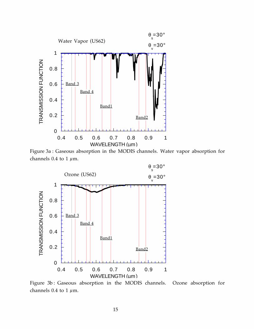
The MODIS instrument contains several features which will help make theatmospheric correction algorithm more accurate than in the past. Most important isthe availability of seven channels in the spectral interval 0.41-2.1 µm that enable thederivation of aerosol loading or aerosol optical thickness. (See Kaufman and Tanr�,1996). Therefore, we can attempt an accurate atmospheric correction for aerosolscattering and absorption at every geographic location. This is an improvement towhat was possible in the past and a direct result from increasing the number ofreflectance channels from two in the AVHRR to seven in MODIS (Salomonson etal., 1989).

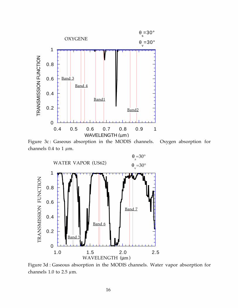
Another important innovation is the smaller bandwidths in the reflectancechannels which avoid overlap with the water vapor absorption bands in all but the0.659 µm and 2.1 µm channels. Therefore, the error introduced by water vaporabsorption is substantially reduced and the need to correct for it is minimized.Figure 3 shows the spectral absorption by water vapor, ozone, oxygen, carbon dioxideand the position of the reflectance channels of MODIS and their respectivebandwidths. Figure 4 shows for MODIS band 2,

Likewise, reducing pixel size from 1 km in the AVHRR to 250 m in MODIS(Salomonson et al., 1989) increases our ability to detect cloudy pixels and reduces thecontamination by subpixel clouds.

Besides the seven reflectance channels, two other MODIS channels areimportant to the atmospheric correction algorithm. The 3.75 µm channel will aid i nthe algorithms for determining aerosol optical thickness. Details are described i nKaufman and Tanr� (1996) . The 1.38 µm channel is vital to detecting thin cirrus andstratospheric aerosols thereby making it possible to correct for these phenomena forthe first time.

15

0

0.2

0.4

0.6

0.8

1

0.4 0.5 0.6 0.7 0.8 0.9 1

Water Vapor (US62)T

RA

NS

MIS

SIO

N F

UN

CT

ION

Band1

Band2

Band 3

Band 4

WAVELENGTH (µm)

θs=30°

θv=30°

Figure 3aÊ: Gaseous absorption in the MODIS channels. Water vapor absorption forchannels 0.4 to 1 µm.

0

0.2

0.4

0.6

0.8

1

0.4 0.5 0.6 0.7 0.8 0.9 1

Ozone (US62)

TR

AN

SM

ISS

ION

FU

NC

TIO

N

Band1

Band2

Band 3

Band 4

WAVELENGTH (µm)

θs=30°

θv=30°

Figure 3bÊ: Gaseous absorption in the MODIS channels. Ozone absorption forchannels 0.4 to 1 µm.

16

0

0.2

0.4

0.6

0.8

1

0.4 0.5 0.6 0.7 0.8 0.9 1

OXYGENET

RA

NS

MIS

SIO

N F

UN

CT

ION

Band1

Band2

Band 3

Band 4

WAVELENGTH (µm)

θs=30°

θv=30°

Figure 3cÊ: Gaseous absorption in the MODIS channels. Oxygen absorption forchannels 0.4 to 1 µm.

0

0.2

0.4

0.6

0.8

1

1.0 1.5 2.0 2.5

WATER VAPOR (US62)

TR

AN

SMIS

SIO

N F

UN

CT

ION

Band 5

Band 6

Band 7

θs=30¡

θv=30¡

WAVELENGTH (µm)Figure 3dÊ: Gaseous absorption in the MODIS channels. Water vapor absorption forchannels 1.0 to 2.5 µm.

17

0

0.2

0.4

0.6

0.8

1

1.0 1.5 2.0 2.5

CARBON DIOXYDET

RA

NSM

ISSI

ON

FU

NC

TIO

N

Band 5

Band 6

Band 7

θs=30¡

θv=30¡

WAVELENGTH (µm)Figure 3eÊ: Gaseous absorption in the MODIS channels. Carbon dioxide absorptionfor channels 1.0 to 2.5 µm.

0.93

0.94

0.95

0.96

0.97

0.98

0.99

1.00

0 1 2 3 4 5 6

tH2O

- MODIS- Band 1

m=3m=5.8m=2

Tran

smis

sion

Water Content (g/cm2)

Figure 4aÊ: Transmission of water vapor in MODIS band 1 vs water vapor contentfor a set of air mass

18

0.93

0.94

0.95

0.96

0.97

0.98

0.99

1.00

0 1 2 3 4 5 6

tH2O

- MODIS- Band 2

m=2m=3m=5.8

Tran

smis

sion

Water content (g/cm2)

Figure 4bÊ: Transmission of water vapor in MODIS band 2 vs water vapor contentfor a set of air mass

0.80

0.85

0.90

0.95

1.00

0 1 2 3 4 5 6

tH2O

- MODIS- Band 7

m=2m=3m=5.8

Tran

smis

sion

Water content (g/cm2)

Figure 4cÊ: Transmission of water vapor in MODIS band 7 versus water vaporcontent for a set of air mass

3. Algorithm Description

3.1 Theoretical background

In this section we describe the algorithms which will make the atmospheric

19

corrections for gaseous scattering and absorption, aerosol scattering and absorption,cirrus contamination, BRDF coupling and the adjacency effect. Figure 5 gives anoverview of the processing chain. Because the atmosphereÕs gaseous compositionwill be relatively known, we propose that the correction for gaseous scattering andabsorption be implemented at launch. However, the correction for aerosol effectsdepends on other MODIS products as input which should be evaluated beforeemployment in the atmospheric correction scheme. Thus we would, at launch,implement an aerosol correction based on the regionally dependent climatologicalaerosol loading ÒclearÓ days. Further details are given in Section 3.1.2 undertropospheric aerosol . A simple, first-order cirrus correction scheme will beimplemented at launch, with more sophisticated techniques replacing it post-launch. Both correction for BRDF coupling and correction for surface adjacencyeffects, which are part of the at-launch algorithm, will only be activated when theother part of the algorithms and the interface with the aerosol product are fullytested and quality controlled.

20

Figure 5Ê: Version 1 atmospheric correction processing thread flow chart. Times aregiven for running on a 195 Mflops processors.

Atmosph er eLU T

,

MODISaerosol

MODIS L1B 1 granule5 minutes of observation

atmospheric correctionfor Lambertian and uniform surface

5 minutes CPU

493 Mb

MODIS water vapor

MODISOzone

Ancillarypressure

10 Mb

Cloud Mask Product

Geolocation product

45 Mb

58 Mb

398 Mb

Aerosol,Water VaporOzone, pressure Climatology

MODIS BRDFproduct

9 Mb

9 Mb

566 Kb

Ancillary Water vapor

Ancillary Ozone

9 Mb

28 Mb

BRDF coupling correctionBoston Coupling LUT

Montana Coupling LUT

26 Mb

311 Mb

26 Mb

adjacency effect correction

Surface Reflectance

Surface Reflectance

Surface Reflectance

21

3.1.1 Physics of the Problem

The radiance in the solar spectrum which reaches the MODIS instrument atthe top of the atmosphere valid for lambertian surface reflectance, can be describedas

L LT T F

STOAs

s

µ µ φ µ µ φµ µ µ ρ µ µ φ

π ρ µ µ φs v s vs v s s v

s v

, , , ,( ) ( ) , ,

, ,( ) = ( ) + ( )

− ( )[ ]00

1(1)

where LTOA is the radiance received by the satellite at the top of the atmosphere, Lois the path radiance, T(µs) is the total transmittance from the top of the atmosphereto the ground along the path of the incoming solar beam, T(µv) is the total

transmittance from the ground to the top of the atmosphere in the view direction ofthe satellite, Fo is the solar radiance at the top of the atmosphere, ρs(µs,µv,φ) is the

surface reflectance with no atmosphere above it, S is the reflectance of theatmosphere for isotropic light entering the base of the atmosphere, µs is the cosine

of the solar zenith angle, µv is the cosine of the view angle and φ is the azimuthal

difference between the two zenith angles. The radiances in Eq. (1) can be normalizedby the incident solar radiance, Foµs/π, which results in the following equation:

ρTOA µs,µv,φ( ) = ρ0 µs,µv,φ( ) +T(µs )T(µv )ρs µs,µv,φ( )

1 − ρs µs,µv,φ( )S[ ] (2)

where ρTOA is the reflectance at the top of the atmosphere and ρo is path radiance

in reflectance units. When T is divided into a direct and diffusive part such that

T(µ) = e-τ /µ + td (µ) (3)

and likewise for T(µs), where τ is the total optical thickness and td the diffuse

transmittance. If the surface is non-Lambertian, the result of the correction using (1)is inexact, due to the coupling between the surface BRDF and atmosphere BRDF notbeing taken into account (Lee and Kaufman, 1986). An approach to model this effectthat stems from the work of Tanre et al (1983) has been implemented in the 6S codeas:

22

ρΤΟΑ θs,θv,φs − φv( ) = ρR+A + e−τ /µv e−τ /µsρs θs,θv,φs − φv( )

+e−τ /µv td µs( )ρ + e−τ /µs td µv( )ρ' + td (µs )td (µv )ρ +TR+A

↓ (µs )TR+A↑ (µv )S ρ( )2

1 − Sρ

(4)

with:

ρ µs,µv,φ( ) =µLR+A

↓

0

1∫

0

2π∫ τΑ ,τR,µs,µ,φ'( )ρs µ,µv,φ' −φ( )dµdφ

µLR+A↓

0

1∫

0

2π∫ τΑ ,τR,µs,µ,φ'( )dµdφ

(5a)

ρ '- (µs,µv,φ) = ρ

- (µv,µs,φ) (5b)

ρ= = Êρ'_ Ê(µs,µv,φ)

_________Ê (5c)

ρ ≅ρs(µ,µ' ,φ)µµ' dµ' dµdφ

0

1∫

0

2π∫

0

1∫

µµ' dµ' dµdφ0

1∫

0

2π∫

0

1∫

(5d)

An important aspect is the validation of the parametrization of the signal which ispresented in Figure 6 where the parametrization of equation (4) is compared versusthe complete computation of the successive order of scattering that include a non-lambertian boundary conditions (Deuze et al, 1989).

23

0.00

0.02

0.04

0.06

0.08

0.10

-60 -40 -20 0 2 0 4 0 6 0

molecules (τr=0.0957)

molecules and aerosols (τr=0.0957,τ

a=0.26)

molecules and aerosols (τr=0.0957,τ

a=0.52)

SOS computations

Figure 6Ê: Comparison of the sum of the atmosphere-BRDF coupling termscomputed using 6S and the same quantity computed by the Successive Order ofScattering code for different atmospheric conditions (clear, average, turbid). Theground BRDF is from Kimes measurements over a plowed field fitted with HapkeBRDF model. The x axis is the view zenith angle in the principal plane, the valuesare negative for back-scattering and positive for forward scattering.

To account for BRDF function provided, quantities in (5a-d) can be computed andthe surface reflectance by solving a second degree equation, the details are given i nthe implementation section.

In case of heteregeneous landscape, at the resolution of the finest MODIS band(250m) we have to consider adjacency effects. Adjacency effects occur when adifferent but adjacent land cover influences the satellite measured radiance of agiven land cover due to atmospheric scattering. The case of inhomogeneous groundboundary conditions has been addressed by several researchers ( Tanr� et al, 1979;Kaufman, 1982; Mekler and Kaufman, 1980; Vermote, 1990). The approach is toassume that the signal received by the satellite is a combination of the reflectance ofthe target pixel and reflectances from surrounding pixels, each weighted by theirdistance from the target

24

The correction procedure stems from the modeling work by Tanr� et al (1981) and issimplified in this code for operational application. When taking into account theadjacency effect, the signal at the top at the atmosphere can be rewritten by

decoupling the photons coming directly from the target ( e− τ

µv ) from those comingfrom areas adjacent to the target and then scattered to the sensor (td(µv)) :

ρTOA = ρR+A +ρsTR+A(µs )e

− τµv + ρs TR+A(µs )td (µv )

1- ρs SR+A(6)

where ρs is the pixel reflectance and <ρs> is the contribution of the pixel background

to the top of the atmosphere signal that is computed as:

ρs = f(r(x,y))ρ(x,y)dxdy−∞

+∞∫

−∞

+∞∫ (7)

where x,y denote the coordinate to a local reference centered on the target, and f(r) isthe atmospheric point spread function.

3.1.2 Implementation of the Algorithm

LUT approach

The quantities ρo(µs,µv,φ), td µ( ) and S are functions of the optical thickness

(τ), single scattering albedo (ω), and phase function (P(θ)) of the scatterers andabsorbers in the atmosphere. The calculation of ρo(µs,µv,φ), td µ( ) and S is achieved

with the aid of an atmospheric radiative transfer program such as the Dave andGazdag (1970) model. However, it is computationally prohibitive to run a radiativetransfer model for every pixel in a daily global data set. Thus, we create a look-uptable with the 6S code (Vermote et al., 1997) which will supply the neededρo(µs,µv,φ), td µ( ), S for a variety of sun-view geometries and aerosol loadings.

ρo(µs,µv,φ) are precomputed 73 relative azimuth angles, 22 solar zenith angles, 22

view zenith angles and 10 aerosol optical depth. td µ( ) is precomputed for 16 zenith

angles and 10 aerosol optical thickness. S is precomputed for 10 aerosol opticalthickness.

25

The radiative transfer computations are dependent on the model inputs.These are discussed below.

Rayleigh Scattering

Scattering by the gaseous constituents of the air is a well-defined problemdepending only on the wavelength of the radiation, air pressure and temperatureprofiles. In the radiative transfer code pressure and temperature profiles are givenby McClatchey (1971) where different profiles are described for various climaticregions and seasons. Surface altitude information for each pixel will be availablethrough a digital elevation model at the resolution of 5 minutes (ETOPO5). This isroughly 8 km by 8 km. The mathematical procedure for Rayleigh scattering is givenin Appendix A. The algorithm will assume a surface elevation of 0 km for use bythe radiative transfer code and adjust the Rayleigh outputs in the look-up table forvariations in elevation and Global Assimilation Model output if available (Fraser etal, 1989; Fraser et al., 1992).

Tropospheric Aerosol

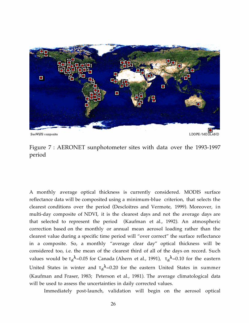
Quality of the surface reflectance estimates is strongly driven by theknowledge of the aerosol optical thickness. The algorithm will use the MODISaerosol product (Kaufman and Tanr�, 1998). At launch, we will use an aerosoloptical thickness data set that we are developing. The data set will consist ofmonthly values interpolated to a 5¡ by 5¡ grid. It will be based on tabulations ofdÕAlmeida (1991) modified with additional data from ground-based sunphotometermeasurements, in particular the Aerosol Robotic Network (Holben et al., 1998) andfrom the literature. Figure 7 shows the AERONET sites (about 130) where data werecollected between 1993 and 1998.The aerosol optical thickness will also be derived from remote sensingmeasurementsÊ: the Advanced Very High Resolution Radiometer (AVHRR) andSea-viewing Wide Field-of-view Sensor (SeaWiFS) data. Such a database isparticularly useful to determine geographic and temporal aerosol patterns. It will beprofitable also for the quality assurance (QA) analyses (see section 3.2.4).

26

Figure 7 : AERONET sunphotometer sites with data over the 1993-1997period

A monthly average optical thickness is currently considered. MODIS surfacereflectance data will be composited using a minimum-blue criterion, that selects theclearest conditions over the period (Descloitres and Vermote, 1999). Moreover, i nmulti-day composite of NDVI, it is the clearest days and not the average days arethat selected to represent the period (Kaufman et al., 1992). An atmosphericcorrection based on the monthly or annual mean aerosol loading rather than theclearest value during a specific time period will Òover correctÓ the surface reflectancein a composite. So, a monthly Òaverage clear dayÓ optical thickness will beconsidered too, i.e. the mean of the clearest third of all of the days on record. Such

values would be τaλ=0.05 for Canada (Ahern et al., 1991), τaλ=0.10 for the eastern

United States in winter and τaλ=0.20 for the eastern United States in summer

(Kaufman and Fraser, 1983; Peterson et al., 1981). The average climatological datawill be used to assess the uncertainties in daily corrected values.

Immediately post-launch, validation will begin on the aerosol optical

27

thickness derived from other MODIS algorithms (Kaufman and Tanr�, 1996). Assoon as it is determined where and when accurate aerosol optical thicknesses areproduced, these new data will be used as input into the atmospheric correctionalgorithm. The MODIS-derived data will enable us to correct for the aerosol loadingdirectly for the specific day and location, and will be a significant improvement tousing the aerosol loading of climatological data. The correction will be applied toregions and periods of time where and when τa is available which is expected to be

areas near dark, dense vegetation. This improvement will be implemented post-launch after the aerosol algorithms are evaluated. Climatological data will continueto be used where there are spatial and temporal gaps in the τa.

The remaining aerosol characteristics needed for the radiative transfer

program are the single scattering albedo, ωoaλ and the phase function, Paλ(θ,z).

These will come from aerosol models appropriate for season and location (Shettleand Fenn, 1979).

Figure 8: composite aerosol optical thickness at 550nm during the week 09/03/93-09/09/93, derived from NOAA AVHRR Global Area Coverage (GAC) data.

28

Stratospheric Aerosol

The stratosphere may at times have a significant optical thickness due tovolcanic eruptions. These aerosol layers may cover a large portion of the globe andpersist on the time scales of months to years. This phenomena can seriouslycompromise vegetation monitoring. An example is the Pinatubo eruption of 1991(Vermote et al, 1994). The stratospheric aerosol optical thickness may be determinedfrom MODIS algorithms using the 1.38 µm channel (Kaufman and Tanr�, 1996) or itmay be provided from other sources e.g. Stratospheric Aerosol and Gas Experiment(SAGE) instrument (McCormick and Vega, 1992). The stratospheric phase functionwill be obtained from King et al. (1984) who used El Chichon data to determine the

properties of volcanic aerosol in the stratosphere. The single scattering albedo, ωosλ,

for the stratospheric aerosol will be computed from the refractive indices tabulatedby Lenoble (1993).

Not only must τa be determined for the column, but it must be decoupled

into stratospheric and tropospheric components. During an important volcaniceruption (e.g. Mt Pinatubo, figure 14) interpreting the aerosol as being locatedentirely in the troposphere will result in errors on the order of up to severalhundredths in reflectance units.

29

50° North

50° South

1981

1993

El Chichon

Pinatubo

Figure 9: Monthly average of the stratospheric aerosol optical depth deduced from

AVHRR data showing major eruptions of El Chichon and Pinatubo.

Gaseous Absorption

To account for gaseous absorption, the reflectance at the top of the atmosphere,ρTOA(µs,µv,φ) is modified as:

ρ θ θ φ φρ ρ ρ

θ θρ

ρ

TOA s v v

R RH O H O

s vs

s

H OH O

Tg O O CO m

Tg MU

T TS

Tg M U

, , , , ,

,

,s −( ) = ( )

+ −( )

+ ( ) ( )− ( )

↓ ↑

3 2 2

02 2

2

2

2

1

(8)

with ρR the molecular intrinsic reflectance, M is the air mass, given byÊ:

Ms v

= +1 1µ µ

30

Tg(O3,O2,CO2,M) is the gazeous transmission of O3, O2 and CO2 , TgH2O

is the water

vapor transmission.The 6S radiative transfer model is used to calculate the gazeous transmission foreach gas in each land bands for a range of total amount of gas and a range of viewangles.

Tg O3,M exp aMUO3( ) = −( ) (9a)

where UO3 is the total amount ozone in units of cm/atm.a is a coefficient which depend on the response of the given spectral band. Detailscan be found in Tanr� et al. (1990).

The formula adopted for oxygen and carbon dioxide is :

Tg Mp

paMb

cp

pd

pp

,0

11

10 0

2 1

= +

+ +

−

p is the pressure at the altitude z and p0 is the pressure at sea level. Oxygen andcarbon dioxide are taken to be constant and are given in units of parts per billion,their amount is directly provided by the altitude. The parameters a,b,c,d are adjustedfor the MODIS spectral responses.

The total precipitable water UH2O [g/cm2] is a MODIS product (Gao andKaufman,1993). It is assumed that the path radiance, ρo, is generated above the

middle of the boundary layer. Thus the additional attenuation is made by half theprecipitable water. The formula adopted for the water vapor transmission is:

Tg H O,M exp e2( ) = − + ( ) + ( )[ ]

xp a b MU c MUH O H Oln ln2 2

2 (9b)

with a,b,c adjusted for the MODIS spectral responses.

Fig. 3 shows that correction for gaseous absorption is only important to bands1 and 4 for ozone and bands 1, 2 and 7 for water vapor. MODIS-derived values oftotal column O3 and H20 will be used as inputs.

31

Cirrus Correction

Correcting for cirrus effects may take several layers of implementation. Alllevels of cirrus correction rely on the MODIS 1.38 µm channel to detect cirrusclouds. This channel is nearly completely absorbed by water vapor in the lowest 6km of the atmosphere. Thus, reflectances measured by this channel are almostexclusively high level clouds (Gao et al., 1993). The zero-order cirrus correction issimply a cloud mask in which all pixels identified as contaminated by cirrus usingthe 1.38 µm channel will be flagged as such. Such procedures are part of the cloudmask products and beyond the scope of this document. However, because thincirrus transmits most of the radiance to and from the surface, it acts in a similarmanner to other atmospheric constituents such as aerosols and should be addressedby atmospheric correction algorithms.

Rather than throwing out all cirrus-contaminated pixels, we intend toeliminate only those pixels where the reflectance in 1.38 µm exceedes apredetermined threshold. Contaminated pixels below that threshold wouldundergo a correction and be used to determine surface reflectance. The simplestcorrection would be to assume that the cirrus reflectance has no spectral dependenceand is spatially homogeneous in a range of 20 km. Therefore, we could correct allchannels with a simple subtraction:

ρλ (µs,µv,φ) = ρλ (µs,µv,φ) − ρ1.38(µs,µv,φ)T1.38

(10)

where ρλ(µs,µv,φ) is the reflectance at wavelength λ and ρ1.38(µs,µv,φ) is the

reflectance measured at 1.38 µm and T1.38 the transmission of water vapor on the

height of the cirrus cloud 0.6±0.2. The subtraction has the added advantage oftransforming a systematic bias to random error.

An even more sophisticated technique would be to correct for cirrusadjacency effect and inhomogeneity. Ice clouds have strong forward scatteringthereby affect path radiance of adjoining pixels which are otherwise cloud-free.Cirrus inhomogeneity is even more important. Pixels viewed by the satellite ascloud free may be illuminated by radiance which transversed cirrus. Thus thesurface reflectance would be in the cirrus ÒshadowÓ although the ÒshadowÓ of thin

32

cirrus may escape cloud shadow masking techniques. This would produceerroneous values for the surface reflectance. The correction of cirrus adjacency andinhomogeneity effects presents an interesting problem that will be left to futureresearch and development.

Surface Adjacency Effect

In the previous processing step, we obtained a corrected reflectance assuminguniform target that is, ρs

ae , which is computed from:

ρ ρ ρ µ µρTOA R+A

s v

1-= + + +

+

sae

R A R A

sae

R A

T T

S

( ) ( )

(11)

We can see that if we consider that: 1

1- ρs SR+A≅ 1

1- ρsSR+A , then ρs and ρs

ae are

related through the following equation:

ρsae = ρs

e− τ

µv

T(µv )+ ρs

td (µv )T(µv )

(12)

therefore, we can correct the reflectance obtained in the previous step, ρsae for the

adjacency effect using:

ρs =ρs

aeT(µv ) − ρs td (µv )

e− τ

µv

(13)

with td (µv ) = TR+A(µv ) − e− τ

µv , with τ=τA+τR

In practice, <ρs> is computed from a sub-zone of 21x21 pixels of the original image

centered on the pixel to be corrected usingi:

iwe here used ρs

ae (i, j) instead of ρs(i,j) since the latter is not available, the error introduced can be reduced by using

33

ρ ρs i, j)==−=−∑∑ f r i j s

ae

ij

( ( , )) (10

10

10

10

(14)

with r(i,j) representing the distance between the pixels (i,j) and the center of thezone.

In practice, the computation as denoted in equation (14), may involve up to 441floating point multiplications, even if tabulated values of f(r(i,j)) are used. This willincrease the amount of megaflops needed for atmospheric correction by a factor of400. We have therefore developed and tested a practical approach to the problemapplied to TM images for a moving window of 41x41 pixels. Two optimizationswere necessary to arrive at an acceptable processing time (about twice the amount oftime of a simple correction). First, we generated over the range of expected values atable of the product f(r(i,j)) ρs

ae(i, j) . By using that table we donÕt perform any

multiplication to compute (14) and reduce the processing time significantly.Secondly the computation for pixel ρs k l,( ) was computed from ρs k l, −( )1 , the

advantage being that the atmospheric point spread function is rather smooth andthat the difference matrix between two adjacent pixels contains many zeroes. Byperforming a sort of the difference matrix and eliminating the zero elements, wewere further able to reduce the number of operations to be performed by roughly afactor of 10.

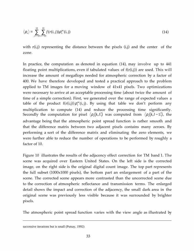
Figure 10 illustrates the results of the adjacency effect correction for TM bandÊ1. Thescene was acquired over Eastern United States. On the left side is the correctedimage, on the right side is the original digital count image. The top part representsthe full subset (1000x1000 pixels), the bottom part an enlargement of a part of thescene. The corrected scene appears more contrasted than the uncorrected scene dueto the correction of atmospheric reflectance and transmission terms. The enlargeddetail shows the impact and correction of the adjacency, the small dark area in theoriginal scene was previously less visible because it was surrounded by brighterpixels.

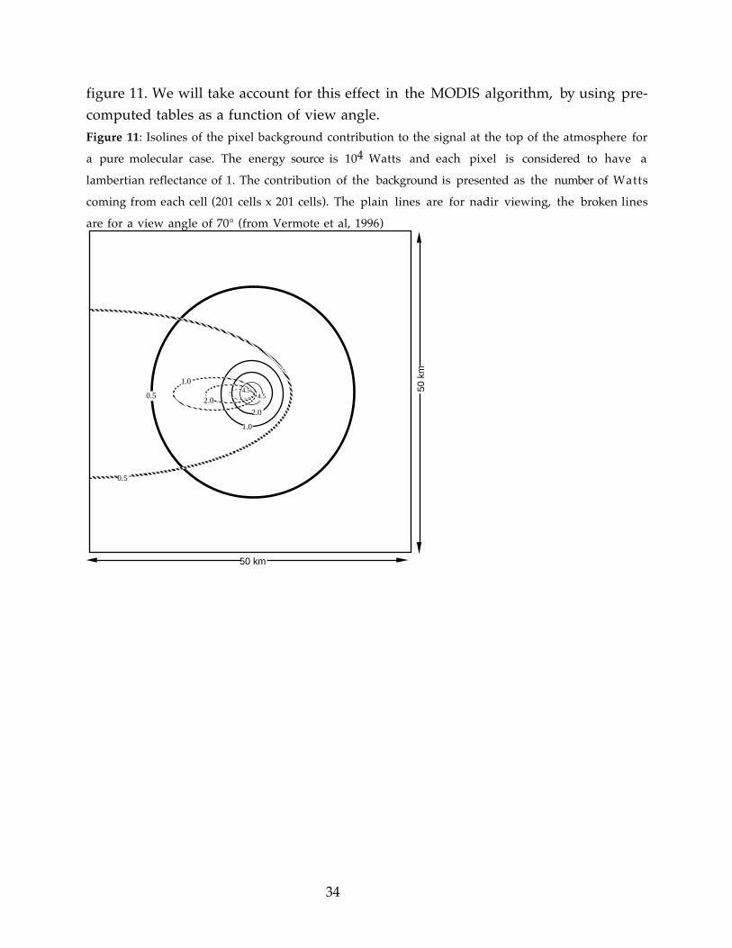
The atmospheric point spread function varies with the view angle as illustrated by

successive iterations but is small (Putsay, 1992)

34

figure 11. We will take account for this effect in the MODIS algorithm, by using pre-computed tables as a function of view angle.Figure 11: Isolines of the pixel background contribution to the signal at the top of the atmosphere for

a pure molecular case. The energy source is 104 Watts and each pixel is considered to have a

lambertian reflectance of 1. The contribution of the background is presented as the number of Watts

coming from each cell (201 cells x 201 cells). The plain lines are for nadir viewing, the broken lines

are for a view angle of 70¡ (from Vermote et al, 1996)

0.5

0.5

1.0

1.0

2.04.5

2.0

4.5

50 km

50 k

m

35

Figure 10: Comparison of TM band 1 data corrected for atmosphere (left side) touncorrected counts (right side). The correction includes adjacency effect correction.

Spatial Grid

The aerosol loading will be calculated from MODIS products on a 10 km by 10km grid over land. The digital elevation model has a resolution of 5 minutes whichis roughly 8 km by 8 km. It is unnecessary to calculate the correction parameters:ρo(µs,µv,φ), td µ( ), L↓ (µ,µ' ,φ' ) and τ, on a higher resolution than the given input

parameters. Thus the correction will be calculated for a spatial grid of 8 km by 8 k m

36

in complex terrain and perhaps as coarse a grid as 10 km by 10 km in flat terrain.

Correction for Non-Lambertianeity

We use the ratio between the estimated BRDF (ρsm ) and the actual surface BRDF (ρs)

to correct the measured values. We rewrite equation (7) as:

ρ µ µ φ ρ ρ µ µ φ

ρ µ µ φ

µ ρ µ ρ µ µ ρ

ρ µ µ φµ µ

τ

τ µ τ µ

ΤΟΑ s vM

s s v

s s v

d s d v d s d v

s s v

R A s R A v

e

e t e t t t

T T

v s

, , , ,

, ,

' ( ) ( )

, ,( ) ( )

/ * / * *

( ) = + ( )

+ ( )( ) + ( ) + +

( )

−

− −

+↓

+↑

0

SS

S

ρ

ρ

*( )−

2

1

(15)

with:

ρ* µs,µv,φ( ) =ρ µs,µv,φ( )

ρsm µs,µv,φ( ) (16a)

ρ' * µs,µv,φ( ) = ρ* µv,µs,φ( ) (16b)

ρ* µs,µv,φ( ) =ρ µs,µv,φ( )

ρsm µs,µv,φ( ) (16c)

When using (15) to retrieve, ρs we have to solve a second degree equation which

only has one positive solution

To compute the different terms (16a-c), we have to use a BRDF model. We have twoapproaches for obtaining modeled BRDF inputs implemented on the version 1 code.

The first solution is to use the bidirectional reflection function that will beprovided on a 1 km by 1 km grid, for the previous 16-day period (Strahler etal.,ATBD, 1996). Results show that the simple assumption for BRDF is sufficient andthat the results are greatly improved versus the lambertian correction. This BRDF is

expected to depend on vegetation index and thus we can fit a F(ρ*,ρ' *,ρ*, ρ) curve

through five selected points in each group of sixty-four 1 km squares defined by our

37

larger 8 km by 8 km grid. These five points will be selected to span the range ofvegetation index values found in the larger grid square eliminating the need forextrapolation. Thus, for any value of vegetation index encountered in the larger grid

square, a value of the coupling term, F(ρ*,ρ' *,ρ*, ρ), can be determined using the

derived equation for the curve fit. In this way, both the atmospheric correction andthe correction for the Lambertian assumption can be applied to each individualpixel within the correction grid square, including pixels at the 250 m resolution.

The second solution is to use a generic BRDF model look-up-table based onruns from the Mymeni et al. three-dimensional canopy model (1992). The BRDF isdepending on the land cover categories used in the MODIS LAI/FPAR product(Running et al., 1994). BRDF and coupling terms are stored in tables as a function ofzenith angles, aerosol optical thickness, biome type and LAI. The biome isdetermined by the land cover map, and the LAI is selected by minimizing thedifference between the spectral dependance of observed and modeled reflectance i nMODIS bands 1,2,3 and 4.

Algorithm Summary

1) On a scale of 5 km by 5 km, we use µs, µv, φ, τa (the aerosol optical thickness), τs(the optical thickness of the stratosphere), τr (the Rayleigh optical thickness), an

aerosol model and look up tables to generate ρR(µs,µv,φ),ρo(µs,µv,φ),), td µ( ), S. Use

elevation to adjust Rayleigh component of the look-up variables.-at launch: τa taken climatology;

τs taken from SAGE data.

-post launch: τa taken from MODIS algorithm where available and

climatology where not; τs taken from MODIS algorithm.

2) For every 5 km by 5 km grid square, compute gaseous absorption correction usingprecipitable water vapor calculated from MODIS algorithms and Eqs. (8-9).

3) For every 5 km by 5 km grid square, look up the equation for F(ρ*,ρ' *,ρ*, ρ) the

bidirectional coupling reflection function, dependent on vegetation index.-at launch: using land cover approach (To be confirmed)

38

-post launch: function determined dynamically from MODIS and MISR products. (in collaboration with Alan Strahler)

4) For every pixel, use the equation found in step 3 to calculate F(ρ*,ρ' *,ρ*, ρ), then

use Eqs (16) to correction for BRDF/ATM coupling effect (if using dynamic BRDF)

5) For every pixel, adjust for cirrus effect, using values at 1.38 µm. -at launch: Use Eq. (10 )-post launch: more sophisticated technique

6) For every pixel, solve Eq. (15) for ρ(µs,µv,φ), the surface reflectance.

7) For every pixel, adjust for adjacency effect. -at launch: no correction-post-launch: implemented when other corrections are tested.

8) Results are surface reflectances for seven wavelengths at every pixel.

3.1.3 Uncertainty Estimates

Uncertainty arises in the atmospheric correction procedure from manydifferent sources. Each of these sources of error will be discussed separately. A nerror budget is presented for 6 different land cover type, those results were obtainedusing the input parameters uncertainties estimate and running the 6S code(Vermote et al., 1997). The code is available on anonymous ftp(address:kratmos.gsfc.nasa.gov). The six different land cover type were simulatedusing a spectral directional model available in 6S (Kuusk, 1994). The parameters ofthe surface model used in the simulation are given in table 2. The complete set ofresults is given in appendix B.

39

Cropland/Grasses Shrubs BroadleafCrops

Savanna LeafForest

NeedleForest

LAI 3.0 3.0 3.0 3.0 3.0 3.0CAB 30.0 30.0 30.0 30.0 30.0 30.0Cw 0.02 0.01 0.03 0.015 0.03 0.015Sl 1.0 0.1 0.5 1.0 0.01 0.01N 1.225 1.225 1.225 1.225 1.225 1.225cn 1.0 1.0 1.0 1.0 1.0 1.0s1 0.4 0.8 0.1 0.4 0.4 0.4θm 70.0 40.0 40.0 70.0 10.0 10.0ε 0.9 0.05 0.05 0.1 0.1 0.1

Table 2: Parameters of the surface model (Kuusk, 1994) used in the error sensitivitystudy. LAI is the Leaf Area Index, CAB is the leaf pigment concentration in unit ofµg/cm2, Cw is the leaf liquid content in unit of cm, Sl is the ratio of the mean chord

lenghts of the leaves by the heigth of the canopy, N is the effective number ofelementary layers inside a leaf, cn is the ratio of refractive indices of leaf surface waxand internal material, s1 is the weight of the price function for soil albedo (s1=0.1 fordark soil, 0.8 for bright soil), θm and ε describe the angular distribution of leavesaccording to an elliptical distribution model where θm is the modal leaf inclinationand ε is the eccentricity of the elliptical distribution of the leaf normals.

Radiative Transfer

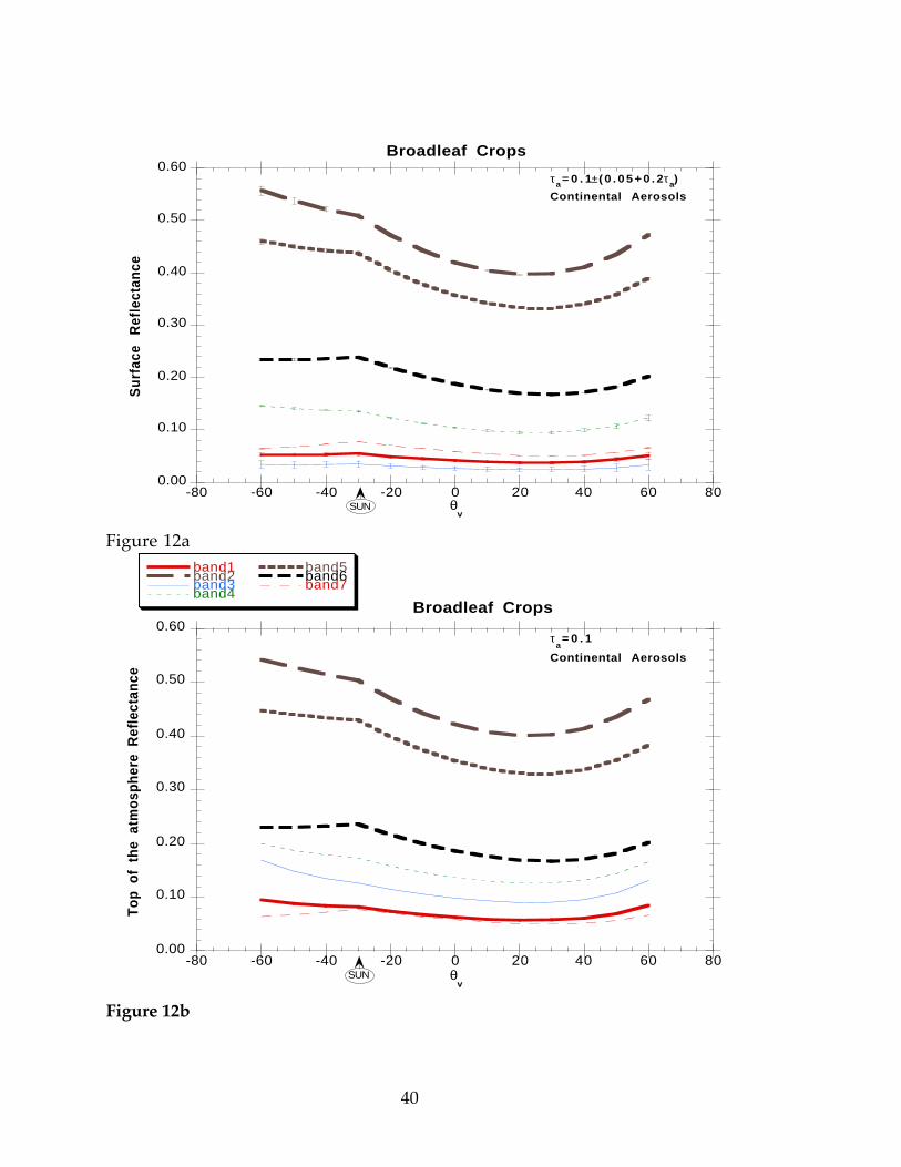
The 6S code was compared to other radiative code like Dave and Gazdag(1970) code. The 6S that does not have the errors associated with molecular-aerosolcoupling that some approximation models have (Herman et al., 1971). It isextremely accurate up to the limits of the plane parallel approximation (about 80o).Angles of this magnitude will only be encountered in the polar regions. Thecurrent version doesnÕt account for polarization that is important at shortwavelength (band 3,4), but the version we plan to use for generating the table foratmospheric will account for polarization. Figure 12a,b shows the importance of theatmospheric effects on different MODIS bands (gaseous absorption excluded), (a)shows the surface reflectance that should be compared to (b) the top of theatmosphere reflectance for a clear atmosphere.

40

0.00

0.10

0.20

0.30

0.40

0.50

0.60

-80 -60 -40 -20 0 20 40 60 80

Broadleaf CropsS

urfa

ce

Ref

lect

ance

θv

τa= 0 . 1±( 0 . 0 5 + 0 . 2τa)

Continental Aerosols

SUN

Figure 12a

0.00

0.10

0.20

0.30

0.40

0.50

0.60

-80 -60 -40 -20 0 20 40 60 80

Broadleaf Crops

band1band2band3band4

band5band6band7

Top

of

the

atm

osph

ere

Ref

lect

ance

θv

SUN

τa= 0 . 1


Figure 12b

41

Absolute Calibration

Uncertainty on absolute calibration will affect the accuracy of the reflectance at thetop of the atmosphere and therefore the corrected reflectance. We simulate an errorof ±2% on the top of the atmosphere reflectance in case ÒaverageÓ aerosol loading(optical depth of 0.3 at 550nm for a continental model) and compute the resultingerror on surface reflectance which we report as error bars. As shown on figure 13,the relative error of 2% could translate to higher error on surface reflectance forbands where atmosphere contribution is much larger than surface contribution,typically under high view zenith angle (>40¡) and in the shortest wavelenghts (band1,3,4).

0.00

0.10

0.20

0.30

0.40

0.50

0.60

0.70

-80 -60 -40 -20 0 20 40 60 80

Grasses/Cereal Crops(calibration uncertainties)

Sur

face

R

efle

ctan

ce

θv

SUN

τa= 0 . 3


Figure 13

42

For a 2% calibration uncertainty, typical relative and absolute errors are:

band rel. error % abs. error

1 4 0.003

2 2 0.015

3 14 0.004

4 3.5 0.004

5 2 0.015

6 2 0.008

7 2 0.003Impact of a calibration error

Input Parameter: τ a

The accuracy of the input parameter, τa is discussed in Kaufman and Tanr�

(1996). We expect an uncertainty of 0.05 for τa derived from MODIS products for

small optical thicknesses and 20-30% for large optical thicknesses. We present Figure14 some simulations of the impact of uncertainties in the aerosol input product.

43

0.00

0.10

0.20

0.30

0.40

0.50

0.60

0.70

-80 -60 -40 -20 0 20 40 60 80

SavannaS

urf

ace

R

efle

cta

nce

θv

τa= 0 . 3±( 0 . 0 5 + 0 . 2τ

a)


SUN

Figure 14

The impact of the uncertainty on surface reflectance retrieval will lead to typicalerrors :

band abs. error of SR

for δA(.55µm)=0.1

abs. error of SR

for δA(.55µm)=0.5

1 0.003 0.008

2 0.008 0.018

3 0.006 0.013

4 0.003 0.007

5 0.007 0.016

6 0.003 0.007

7 0.002 0.004Impact of AOT uncertainty on surface reflectance retrieval (reflectance units)

44

Aerosol Model

The choice of aerosol model which will determine the phase function, Pa(θ),

and single scattering albedo, ωoa, used by the radiative transfer code is an important

source of uncertainty. Presently we can assign aerosol models only according togeographical location, season or aerosol loading. These criteria do not necessarilyproduce accurate representations of the aerosol size distribution or aerosolabsorption. Uncertainty in the input phase function, Pa(θ), can cause uncertainty i n

the correction by as much as 0.02 in reflectance units for a surface reflection of 0.05 asdescribed by Fraser et al. (1989) and Fraser et al. (1992). Uncertainty in the input ωoacaused smaller uncertainties, less than 0.005. For the MODIS aerosol algorithms, τais obtained from path radiance estimations (Lo). In this case the accuracy of the

correction will be better than the accuracy reported above due to a self compensatingerror. We performs sensitivity study to determine the impact of an error on theaerosol model, by correcting with a continental model when the actual aerosol wasdust (background desertic model in 6S) or smoke (biomass burning model in 6S).The three models (continental,dust,smoke) have different phase functions, singlescattering albedos and spectral dependence of extinction coefficients which areexpected to cover the range of actual conditions. The compensation process wastaken into account, as it can be seen on Figure 15a,b, the error on correction ofchannel used to derive aerosols (band 1,3) is relatively small, error in other channelscan be much higher (band 2).

45

0.00

0.10

0.20

0.30

0.40

0.50

0.60

0.70

-80 -60 -40 -20 0 20 40 60 80

Leaf forestsError on aerosol model : Biomass Burning


band5band6band7

Sur

face

R

efle

ctan

ce

θv

SUN

τa= 0 . 3


Figure 15a

0.00

0.10

0.20

0.30

0.40

0.50

0.60

0.70

-80 -60 -40 -20 0 20 40 60 80

Leaf ForestsError on aerosol model : Background Desertic

Sur

face

R

efle

ctan

ce

θv

SUN

τa= 0 . 3


Figure 15b

46

The typical errors estimated are (for δA(.550Êµm)=0.3 and sun zenith angle of 30¡)Ê:

band abs. error

1 0.002

2 0.017

3 0.002

4 0.005

5 0.016

6 0.009

7 0.006Impact of aerosol model uncertainty

Lambertian Approximation Error

This error results from assuming a Lambertian surface and using an equationsimilar to Eq. (2) in place of Eqs. (15,16). The Lambertian approximation error maybe the most important error in the atmospheric correction process. Lee andKaufman (1986) quantify the error due to Lambertian approximation based onradiative transfer simulation at 0.65 and 0.85 µm using ground boundary conditionsfor pasture, forest and savanna as measured by Kriebel et al. (1978). In thebackscattering direction (hotspot) the error ranges from 0.02 to 0.06 in reflectanceunits for a clear atmosphere to 0.03-0.11 for a hazy atmosphere (τa=0.5) for a solar

zenith angle of 60o. The error is smaller outside of the backscattering direction andis expected to be larger at short wavelengths and with increasing solar zenith angle.Figure 16 shows for one case the error produced by the lambertian approximation.Figure 16 also shows the error done (error bars) if we use equations (15,16) with the afirst guess BRDF model, in that case we use a broadleaf BRDF to correct the grassescase. The error is substantially lower than the lambertian approximation.

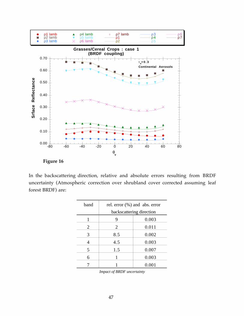
47

0.00

0.10

0.20

0.30

0.40

0.50

0.60

0.70

-80 -60 -40 -20 0 20 40 60 80

Grasses/Cereal Crops : case 1(BRDF coupling)

ρ1 lambρ2 lambρ3 lamb


ρ7 lambρ1ρ2

ρ3ρ4ρ5

ρ6ρ7

Srf

ace

Ref

lect

ance

θv

τ a= 0 . 3


Figure 16

In the backscattering direction, relative and absolute errors resulting from BRDFuncertainty (Atmospheric correction over shrubland cover corrected assuming leafforest BRDF) are:

band rel. error (%) and abs. error

backscattering direction

1 9 0.003

2 2 0.011

3 8.5 0.002

4 4.5 0.003

5 1.5 0.007

6 1 0.003

7 1 0.001Impact of BRDF uncertainty

48

Total theoretical typical accuracy :

band abs. error rel. error %

(range)

1 0.005 10-33

2 0.014 3-6

3 0.008 50-80

4 0.005 5-12

5 0.012 3-7

6 0.006 2-8

7 0.003 2-8

Gaseous Absorption, Polarization, Vertical Distribution

Errors caused by uncertainties in gaseous absorption, polarization, andvertical distribution of aerosols were all found to be less than 0.005 in reflectanceunits for a surface reflectance of 0.05 by Fraser et al. (1989) and Fraser et al. (1992).

Adjacency Effect

The adjacency effect correction gives an approximation which is an exactsolution in the case of a homogeneous background. Application of the correction toSPOT data for a target with reflectance of 0.20 surrounded by a dark backgroundreduces the error from adjacency effect at 550 nm from 0.005 to less than 0.001 i nreflectance units (Vermote, 1990). Because pixel size is larger for MODIS than forSPOT we expect errors from this effect to be even smaller and the final values aftercorrection to have even less error. A complete sensitivity study to address that erroris being done.

Cirrus Effect

We presently do not know the uncertainties involved with using Eq. (10) to

49

correct for cirrus contamination; however, this procedure will translate a systematicbias to random error in the following manner. Ignoring thin cirrus will cause auniversal brightening of surface reflectances. By subtracting the 1.38 µm reflectancefrom the apparent reflectance the surface reflectances are now sometimes too brightor too dark, but the average value is closer to their actual value without the cirruscontamination.

Look-Up Table Interpolation

As explained in section 3.1.2, we created look-up tables with the 6S code tosupply the needed ρo(µs,µv,φ), td µ( ), S for a variety of sun-view geometries and

aerosol loadings. Similar look-up tables are described in Fraser et al.(1989, 1992).Fraser et al. (1992) report that errors in the derived surface reflectance resulting frominterpolation between entries in the look-up table are large only when either sunangle or view angle are extreme (>70¡). Uncertainty caused by interpolation fromthe look-up table were found to cause errors in the corrected reflectance of less than0.005 for surface reflectance of 0.05 (Fraser et al., 1989; Fraser et al., 1992). This look-up table consisted of values for 9 solar zenith angles, 13 view angles, 19 azimuthalangles, and 4 aerosol optical thicknesses. A finer resolution table consisting of 22solar and view zenith angles, and 73 relative azimuth angles reduces theinterpolation error to 0.002 in reflectance units.

3.2 Practical Considerations

3.2.1 Numerical Computation Considerations

Nothing to report

3.2.2 Programming/Procedural Considerations

The atmospheric correction algorithm is a mid-level point in the dataprocessing. The atmospheric correction algorithm is a completely automatedprocedure. The code is written to handle exceptions and errors as they occur.

50

Estimation of the processing time are given on figure 5.

3.2.3 Data dependencies

The atmospheric correction algorithm uses MODIS products as inputs andproduces new products which are in turn used by other MODIS algorithms. TheMODIS-derived products used as inputs include: geographically registered andcalibrated radiances (MOD02, MOD03) cloud mask (MOD35), spectral aerosol opticalthickness (MOD04), precipitable water (MOD05), ozone (MOD07) and surface BRDFproduct from the 16-D prior period (MOD43). Ancillary data include a Digitallevation Model, Data Assimilation Office (DAO) for surface pressure, water vapor,and ozone, climatological data for water vapor, ozone and aerosol optical thickness.

The algorithm makes use of a look-up table which supply the neededρo(µs,µv,φ), td µ( ), BRDF coupling terms, and s for a variety of geometries and

aerosol properties. In this way we avoid the need to run the radiative transfer codefor every pixel, an impossible task in terms of CPU. We calculate ρo(µs,µv,φ), td µ( )and s on a grid of 5 km by 5 km, but will provide the corrected reflectance at everypixel. This further reduces the calculation time.3.2.4 Output product

L2 product:

The MOD09 implemented algorithm will process daily the 7 land bands at 250 m(bands 1 and 2) and 500 m (bands 3-7) (standard DAAC production). The outputproduct contains the estimates of the surface reflectance, QA bit fields and QAmetadata for each data granule. The HDF file for the L2 contains the following SDS :

1-250 m Surface Reflectance Band 1







8-250 m Reflectance Band Quality

9-500 m Reflectance Band Quality

10-1 km Reflectance Data State QA

L2G and L3 products:

51

A level 2G (daily) and a level 3 land (8-day) surface reflectance will be based uponthe Level 2 data. The level 3 is a 8-day composite. The compositing techniquesuggested is based on the minimum-blue criterion that selects the clearestconditions over the period (See prototyping activities).

The surface reflectance is the input for the production of the MODLAND groupÕssurface products: vegetation index, BRDF/surface albedo, land cover change andLAI/FPAR.

3.2.3 Validation

Validation activities can be divided into pre-launch validation of the algorithm andpost-launch validation of the product. Various approaches can be adopted forvalidation. The Surface Reflectance Product validation will use a combination ofground based measurements, airborne measurements, comparison with othersensor data and image analysis.

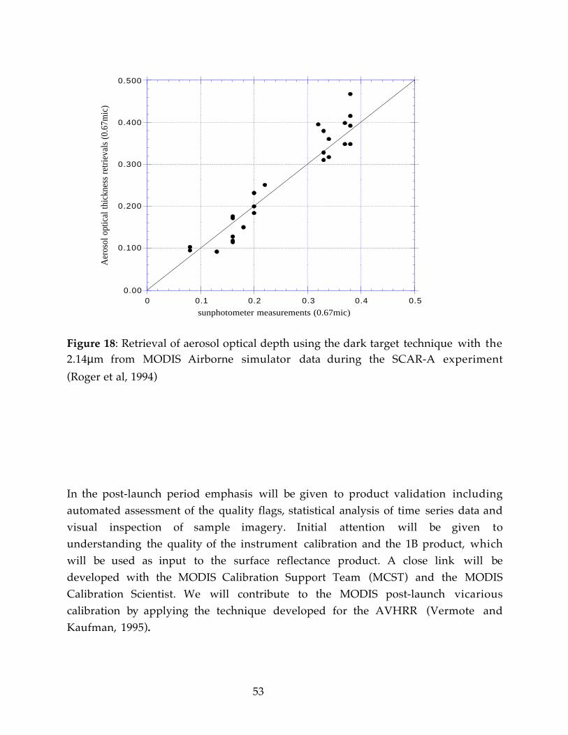
The mainstay of the pre-launch validation of the algorithm will be the use of sunphotometer data collected at a series of test sites with known land covercharacteristics in conjunction with data from existing sensor systems e.g. TM, MASand AVHRR. We will build on the experience developed using theLTER/Sunphotometer atmospheric correction validation project (figure 17). Theproposed algorithm will be prototyped using AVHRR 1km data.. An assessmentwill be made of the algorithm performance and the impact of errors in the aerosolinput product and in using the aerosol climatology. MAS data acquired by the ER2will be used to provide additional validation in bands unavailable on the AVHRR(see figure 18). Flights will be coordinated with other members of the MODIS teamand will require contemporaneous sun photometer data. The existing sunphotometer network is shown in figure 18. Ideally this network will be expanded bythe EOS Validation Program to include sufficient sites to represent the range ofatmospheric conditions and surface types. Advantage will be taken of data suitablefor the algorithm validation collected as part of the NASA intensive fieldcampaigns (e.g. BOREAS and LBA) or through EOS coordinated field validationprograms (e.g. SCAR campaigns). In the pre-launch period, we will also assist i ndefining and testing generic image validation tools suitable for use by the MODIS

52

Science Team planned for development by MODIS SDST, ECS or other instrumentteams e.g. time series video looping.

0.00

5.00

10.00

15.00

20.00

0 .0 0.050 0.10 0.15 0.20 0.25

Histogram of the reflectance observed over Hog Island

Turbid day (corrected)Clear day (Corrected)Turbid day (top of the atmosphere)Clear day (Top of the atmosphere)

Fre

qu

en

cy

TM band 1 reflectance

Figure 17: test of the result of the atmospheric correction procedure (includingaerosol retrieval and atmospheric point spread function correction) for a 1000x1000TM pixels area of the Hog Island site for the clear and hazy day for TM band 1.

53

0.00

0.100

0.200

0.300

0.400

0.500

0 0.1 0.2 0.3 0.4 0.5

Aer

osol

opt

ical

thic

knes

s re

trie

vals

(0.

67m

ic)

sunphotometer measurements (0.67mic)

Figure 18: Retrieval of aerosol optical depth using the dark target technique with the2.14µm from MODIS Airborne simulator data during the SCAR-A experiment

(Roger et al, 1994)

In the post-launch period emphasis will be given to product validation includingautomated assessment of the quality flags, statistical analysis of time series data andvisual inspection of sample imagery. Initial attention will be given tounderstanding the quality of the instrument calibration and the 1B product, whichwill be used as input to the surface reflectance product. A close link will bedeveloped with the MODIS Calibration Support Team (MCST) and the MODISCalibration Scientist. We will contribute to the MODIS post-launch vicariouscalibration by applying the technique developed for the AVHRR (Vermote andKaufman, 1995).

54

The technique relies on using using high altitude (12 km and above) bright clouds as"white" targets for intercalibration between channels in the visible, near infraredrange. Ocean glint can be used at larger wavelengths . Using intercalibration betweena shorter wavelength channel and near infrared, an absolute calibration of firstchannel can be deduced using ocean off-nadir view (40¡-70¡) in channel 1 and 2 andcorrection for the aerosol effect. In this process the second channel to correct aerosoleffect in the first channel 1. Figure 19 shows the results of intercalibration ofchannel 1 and 2 for NOAA7,9,11 using the cloud technique. Figure 20 shows for theresults of the absolute calibration derived for channel 1.

0.9

0.95

1

1.05

1.1

1.15

1.2

1.25

1.3

81 82 83 84 85 86 87 88 89 90 91 92 93

NOAA 7 NOAA 9 NOAA 11

r 12

YearFigure 19: Intercalibration between AVHRR channel 1 and 2, r12 as observed over high reflectiveclouds for NOAA7-9-11 (Vermote and Kaufman, 1995).

55

0.75

0.80

0.85

0.90

0.95

1.00

1.05

0 100 200 300 400 500 600 700 800

Ocean method NOAA 11PATHFINDER I - NOAA11Ocean method - NOAA09PATHFINDER I - NOAA09

Deg

rada

tion

in c

hann

el 1

fro

m p

re-f

light

coe

ffici

ent

Day since 1/1/89 (NOAA11)Day since 1/1/85 (NOAA09)

Figure 20: Absolute calibration of NOAA-9,11 AVHRR channel 1 using the ocean method, Theresults are normalized to the by NOAA pre-flight calibration (Vermote and Kaufman, 1995). Alsoshown is the Pathfinder recommended calibration

In a post launch phases, validation of the MODIS surface reflectance productswill be done at a field campaign level and at a more continuous level throughvalidation sites. Prototype of the validation site are being designed now. Althoughdetails of the validation plan are included in the MODIS Land Validation planavailable on the WWW from the EOS Validation Office, several key points areoutlined here. The MODIS land products will be validated at test sites groupedaccording to a five-tier system. The system is based on the instrumentation andactivities occuring at the sites, and include: 1) intensive field campaign sites (e.g.,FIFE, BOREAS, LBA), 2) fully instrumented sites (e.g., ARM/CART), 3) biome towersites (e.g., Harvard Forest LTER), 4) globally distributed test sites (e.g., NOAA CMDL),and 5) instrument calibration sites (White Sands). The number of sites increasesfrom only a few tier 1 and 2 sites to perhaps 60 tier 4 sites, while the instrumentation

56

and investment per site decreases from tiers 1 and 2 to tier 4.

Full atmosphere and surface characterization generally will be available forthe tier 1 and 2 sites as these typically involve simultaneous sun photometermeasurements, aircraft overflights, and full surface and atmosphere radiometry.Although we will extensively use data from the CIMEL sunphotometer (see below),other instrumentation such as spectrometers and shadow-band radiometersnormally are available at these sites. In addition, vegetation biosphysical variablesare typically well sampled. Although expense prevents a large number of tier 1 and2 sites from being developed or operated over long periods, these sites will presentthe best opportunties for end-to-end product validation and error analysis. Thus,we expect our most comprehensive algorithm testing will completed at these sites,and we will participate as opportunties exist.

Because the few tier 1 and 2 sites will not be able to represent the broad rangeof climate/land cover combinations encountered globally, we will rely on the moreinstrument-limited tier 3 and 4 sites for continuous global validation. Currently, weplan to collaborate existing tower sites maintained under various ÒnetworkÓ studies(e.g., EUROFLUX, LTER, AMERIFLUX, AERONET). To minimize costs, and thusincrease the number of sites, we propose that each tower site include a CIMELsunphotometer (~$20,000) mounted well above the canopy top. With the currentsoftware used in the AERONET sunphotometer network, CIMEL data allowretrieval of the aerosol optical depth and phase function. Augmented with newsurface BRDF software being developed by the CIMEL company and tested byMODLAND, the sunphotometer will measure the surface-leaving radiance over alarge range of view anglesÑincluding the MODIS-view angles. Again using theAERONET model, the data will be uplinked in real-time to a satellite and receivedat our SCF. This abundant data resource will allow continuous evaluation of theaerosol optical depth input to our algorithm, and the BRDF-atmosphere couplingterms (including the bihemispherical reflectance distribution function [BHRF] andthe hemispherical directional reflectance distribution [HDRF], which represents theconvolution of the total irradiance with the surface BRDF). Note the deconvolvedsurface reflectance product cannot be measured independently, and therefore wemust rely on ground-measured HDRF values to validate our algorithm andproduct.

57

The tier 3 and 4 tower configuration, complete with the modified CIMELsampling program, will be rigorously tested in 1997 during two MODLANDprototype validation campaigns. Although the exact sites and times are still underreview, we will set up the tower and ground instrumentation for 10 day periods atboth a tall canopy (e.g., forest) site and a short canopy (e.g., grassland) site. Inaddition, we are scheduling aircraft sensor overflights (e.g., MAS and AVIRIS) andground biophysical characterization (LAI, fAPAR) while collecting the towerinstrument data. These prototype campaigns should expose any problems in ourinstrumentation or sampling scenarios (time or space) in time to modifyprocedures, if necessary, before the actual validation sites are developed. Note thatall MODLAND science teams are participating in these prototype campaigns. Boththe ASTER and MISR teams have expressed interest in collaborating, and uponfinalizing details we expect to involve othersÑincluding the succesful proposers tothe EOS Validation Office Announcement of OpportuntityÑin these activities.

Overall, we expect to have at least 10 tier 3 and 4 sites instrumented andoperating at launch (Phase A), providing an opportunity for immediate productevaluation. Within a year post-launch, we expect to have an additional 10 sitesoperating (Phase B), and hope to complete a network of 80 total sites by the year 2000(Phase C). We are currently developing a list of prefered sites for priorityinstrumentation, and our working closely with the EOS validation office, other AMinstrument teams, and network personnel in our planning. Every effort will bemade to ensure the sites are relatively homogeneous (or Òconstantly mixedÓ), large(at least 2 km x 2 km), and representative of the most spatially extensive and/orbiogeochemically-important landcovers.

3.2.4 Quality Control and Diagnostics

The estimates of the surface reflectance is accompanied with quality assuranceinformation. QA bits contain information stored at the product resolution, whereasQA metadata contain overall statistical information of a whole granule calculatedfrom QA bits. The QA data include information on the integrity of the surfacereflectance estimate, the successful completion of the correction scheme, the cloudcover, the source of aerosol, water vapor and ozone information.QA analyses will be performed over a sample of data at different time scales andspatial resolutions. EOS validation sites will be systematically monitored.

58

A MODIS coarse spatial resolution of the level 2 and the level 3 surface reflectanceproduct have been developed by the SCF for internal QA purposes. These productsare not to be archived and should only be distributed to the GSFC Land SCF or theMODLAND Land Data Operational Product Evaluation Group (LDOPE). Apreliminary QA will be performed every day on these coarse resolution products. Itshould allow a rapid global assessment of the data quality. With the metadata storedLDOPE QA database, it will help the selection of granules or tiles to be ordered fordetailed QA.

The algorithm products will be reviewed post-launch to determine whetherthe corrected surface reflectances are dependent on other variables and in whatmanner. This may give us insights into possible improvements in the algorithm. For example, an ideal atmospheric correction should produce surface reflectancesnot dependent on τa. However, the algorithm we are proposing for bidirectional

effects may not be accurate enough to correct for the dependence between τa and

surface reflectance due to shadows. This effect is stronger in the forward scatteringdirection but almost negligible in the backscattering direction (Deering, 1989). Forthis reason we will look at data only from the backscattering direction in evaluatingthe algorithmÕs dependence on τa. Dependence of corrected surface reflectance on τain the backscattering direction points to errors in the aerosol phase function or toerrors in the single scattering albedo (Fraser and Kaufman, 1985).We developed an Òinvestigative toolÓ that can detect such data dependency. Thistool is based on the 6S radiative code and will be used as a Òflexible MOD09Ó. Itallows modifying some of the input (e.g. aerosol optical thickness, aerosol model). Itwill be very useful to verify that the processing of the L1B data is working correctly(DAAC benchmarking).

3.2.5 Exception Handling

Exception handling will be built into the code. Extreme angles and extremeinput parameters will be flagged. Cloud and cirrus contamination will be noted.Missing data will also be noted.

4. Constraints, Limitations and Assumptions

59

This algorithm is constrained to land areas and will be most accurate i nregions where the aerosol optical thickness is derived from MODIS products. Theseare areas with sufficient dense, dark vegetation. ÒClearÓ climatological values ofoptical thickness still need to be measured in most parts of the world. This factlimits the accuracy of the at-launch algorithm. Furthermore, in the case of animportant volcanic eruption (e.g. Mt Pinatubo) it appears essential that the MODISaerosol product (Kaufman and Tanre,1998) should de-couple the stratospheric andtropospheric aerosol contribution. Errors in de-coupling this product will limit theaccuracy of the derived surface reflectance during volcanic events.Extreme angles, which may be encountered in polar regions may cause large errors.

60

5. Research Agenda

61

REFERENCES

F. J. Ahern, R. P. Gauthier, P. M. Teillet, J. Sirois, G. Fedosejevs and D. Lorente, 1991:An investigation of continental aerosols with high spectral resolution solarextinction measurements. Applied Optics,30,5276-5287.

F. J. Ahern, D. G. Goodenough, S. C. Jain, V. R. Rao and G. Rochon, 1977: Use ofclear lakes as standard reflectors for atmospheric measurements. in Proc. 11th Int.

Symp. on Remote Sens. of Environ., Ann Arbor MI. 731-755.

G. A. d'Almeida, P. Koekpe and E. P. Shettle, 1991: in Atmospheric Aerosols Global

Climatology and Radiative Characteristics. Hampton. A. Deepak Publishing, 561 pp.

J. V. Dave and J. Gazdag, 1970: A modified Fourier transform method for multiplescattering calculations in a plane parallel Mie atmosphere. Applied Optics,9,1457-1466.

D. W. Deering, 1989: Field measurements of bidirectional reflectance. in Theory and

Applications of Optical Remote Sensing, ed. G. Asrar, New York. Wiley & Sons, 734 pp.

P. Y. Deschamps, M. Herman and D. Tanre, 1983: Modeling of the atmosphericeffects and its application to the remote sensing of ocean color. Applied Optics,22,3751-3758.

Descloitres and Vermote, 1999Ê: Operational retrieval of the spectral surfacereflectance and vegetation index at global scale from SeaWiFS data. Proceedings ofthe International Conference and Workshops on Ocean Color, Land Surfaces,Radiation and Clouds, Aerosols, ALPS�99 : The contribution of POLDER and newgeneration spaceborne sensors to global change studies, Land surfaces-O-02

Deuze, J. L., Herman, M. and Santer, R. (1989), Fourier series expansion of thetransfer equation in the atmosphere-ocean system, J.Q.S.R.T. 41(6):483-494.

J. Dozier and J. Frew, 1981: Atmospheric corrections to satellite radiometric data overrugged terrain. Remote Sens. Environ.,11,191-205.

62

El Saleous, N.Z., Vermote, E.F., Justice, C.O., Townshend, J.R.G., Tucker, C.J.,Goward, S.N., 1999, Improvements in the global biospheric record from theAdvanced Very High Resolution Radiometer (AVHRR), International Journal ofRemote Sensing.

R. S. Fraser and Y. J. Kaufman, 1985: The relative importance of scattering andabsorption in remote sensing. IEEE Trans. on Geoscience and Rem. Sens.,23,625-633.

R. S. Fraser, R. A. Ferrare, Y. J. Kaufman and S. Mattoo, 1989: Algorithm foratmospheric corrections of aircraft and satellite imagery. NASA Technical

Memorandum 100751,98 pp.

R. S. Fraser, R. A. Ferrare, Y. J. Kaufman and S. Mattoo, 1992: Algorithm foratmospheric corrections of aircraft and satellite imagery. Int. J. Remote Sensing, 13,

541-557.

B.-C. Gao and Y.J. Kaufman, 1993: Water vapor retrieval from MODIS.

H. R. Gordon, J. W. Brown and R. H. Evans, 1988: Exact Rayleigh scaterringcalculations for use with the Nimbus-7 Coastal Zone Color Scanner. Applied

Optics,27,862-871.

B. M. Herman, S. R. Browning and R. J. Curran, 1971: The effect of AtmosphericAerosols on Scattered Sunlight. J. Atmos. Sci.,28,419-428.

B. N. Holben, 1986: Characteristics of maximum-value composite images fortemporal AVHRR data. International Journal of Remote Sensing,7,1435-1445.

B. N. Holben, E. Vermote, Y. J. Kaufman, D. Tanr� and V. Kalb, 1992: AerosolRetrieval over Land from AVHRR data-Application for Atmospheric Correction.IEEE Trans. on Geosci. and Rem. Sens.,30,212-222.

Holben, B. N., Eck, T. F., Slutsker, I., Tanr�, D., Buis, J. P., Setzer, A., Vermote, E. F.,Reagan, J. A., Kaufman, Y. J., Nakajima, T., Lavenu, F., Jankowiak, I., & Smirnov,A. (1998). AERONET - A federated instrument network and data archive for aerosol

63

characterization. Remote Sensing of Environment, 66(1), 1-16.

R. G. Holm, M. S. Moran, R. D. Jackson, P. N. Slater, B. Yuan and S. F. Biggar, 1989:Surface reflectance factor retrieval from Thematic Mapper data. Remote Sens.

Environ.,27,47-57.

M. E. James, S. N. V. Kalluri and J. R. G. Townshend, 1993: The Pathfinder AVHRRland data set: An improved coarse resolution data set for terrestrial monitoring. Int.

J. Remote Sensing,submitted.

C. O. Justice, J. R. G. Townshend, B. N. Holben and C. J. Tucker, 1985: Analysis of thephenology of global vegetation using meteorological satellite data. Int. J. Remote

Sensing,6,1271-1318.

C. O. Justice, T. F. Eck, D. Tanr� and B. N. Holben, 1991: The effect of water vapouron the normalized difference vegetation index derived for the Sahelian region fromNOAA AVHRR data. Int. J. Remote Sensing,12,1165-1187.

Y. J. Kaufman, 1982: Solution of the equation of radiative transfer for remotesensing over two-dimensional surface reflectivity. J. Geoph. Res.,20,4137-4147.

Y. J. Kaufman, 1987: The effect of subpixel clouds on remote sensing. Int. J. Remote

Sensing,8,839-857.

Y. J. Kaufman and R. S. Fraser, 1983: Light Extinction by Aerosols During SummerAir Pollution. J. Clim. App. Meteor.,22,1694-1706.

Y. J. Kaufman, A. Gitelson, A. Karnieli, E. Ganor, R. S. Fraser, T. Nakajima, S.Mattoo and B. Holben, 1993: Size distribution and phase function of aerosol particlesretrieved from sky brightness measurements. J. Geoph. Res. - A, submitted June.,

Y. J. Kaufman and C. Sendra, 1988: Algorithm for automatic atmospheric correctionsto visible and near-IR satellite imagery. Int. J. of Remote Sens.,9,1357-1381.

Y. J. Kaufman and D. Tanr�, 1992: Atmospherically resistant vegetation index(ARVI) for EOS-MODIS. IEEE Trans. Geosci. Remote Sensing,30,261-270.

64

Kaufman, Y. J., Tanre, D., Remer, L., Vermote, E., A. Chu and Holben, B. (1997),Operational Remote Sensing of tropospheric aerosol over land from EOS moderateresolution imaging spectroradiometer, J. Geoph. Res. Vol. 102, No14, pp17051-17067

Y. J. Kaufman and D. Tanr�, 1998: Algorithm for remote sensing of aerosol fromMODIS. MODIS Algorithm Theoretical Basis Document.

Y. J. Kaufman, D. Tanr�, B. N. Holben, B. Markham and A. Gitelson, 1992:Atmospheric effects on the NDVI - Strategies for its removal. International Geoscience

and Remote Sensing Symposium (IGARSS). Houston, TX. IEEE, 1238-1241.

Kimes, D. S., Newcomb, W. W., Tucker, C. J., Zonneveld, I. S., Van Wijngaarden,W., De Leeuw, J. and Epema, G. F., 1985, Directional Reflectance Factor Distributionsfor Cover Types of Northern Africa. 17, 1-19.

M. D. King, Harshvardhan and A. Arking, 1984: A model of the radiative propertiesof the El Chichon stratospheric aerosol layer. J. Clim. Appl. Meteorol.,23,1121-1137.

K. T. Kriebel, 1978: Measured directional reflection properties of four vegetatedsurfaces. Applied Optics,17,253-259.

Kuusk A. A,1994 a multispectral canopy reflectance model., Remote Sens. Environ.,1994, 50:75-82.

T. Y. Lee and Y. J. Kaufman, 1986: Non-Lambertian effects on remote sensing ofsurface reflectance and vegetation index. IEEE Trans. Geoscience and Rem. Sens., GE-

24,699-708.

J. Lenoble, 1993: Atmospheric Radiative Transfer. Hampton, VA. A. Deepak Publishers,532 pp.

R. A. McClatchey, R. W. Fenn, J. E. A. Selby, F. E. Volz and J. S. Garing, 1971: Optical

properties of the atmosphere. AFCRL-71-0279,Air Force Cambridge Research Lab,Hanscom AFB MA.

65

M. P. McCormick and R. E. Viega, 1992: Sage II Measurements of early PinatuboAerosols. Geophysical Research Letters,19,155-158.

Y. Mekler and Y. Kaufman, 1980: The effect of earth's atmosphere on contrastreduction for a nonuniform surface albedo and two-halves field. J. Geoph.Res.,85,4067-4083.

M. S. Moran, R. D. Jackson, G. F. Hart, P. N. Slater, R. J. Bartell, S. F. Biggar, D. I.Gellman and R. P. Santer, 1990: Obtaining surface reflectance factors fromatmospheric and view angle corrected SPOT-1 HRV data. Remote Sens.

Environ.,32,203-214.

M. S. Moran, R. D. Jackson, P. N. Slater and P. M. Teillet, 1992: Evaluation ofsimplified procedures for retrieval of land surface reflectance factors form satellitesensor output. Remote Sens. Evniron.,41,169-184.

Ouaidrari H., & Vermote E. F. (1999, in press). LANDSAT TM software foratmospheric correction. Remote Sensing of Environment.

J. T. Peterson, E. C. Flowers, G. J. Berri, C. L. Reynolds and J. H. Rudisill, 1981:Atmospheric turbidity over central North Carolina. J. Appl. Meteor.,20,229-241.

Putsay, M. (1992), A simple atmospheric correction method for the short wavesatellite image, Int. J. Remote Sensing 13(8):1549-1558.

S. I. Rasool, 1987: Potential of remote sensing for the study of global change. Advances

in Space Research,7,1-90.

J.C. Roger , Eric Vermote and Nazmi El Saleous., 1994, "Atmospheric Correction ofMAS data during SCAR-A experiment", Atmospheric Sensing and Modeling,Rome, Italy, September 29-30, SPIE proceedings, Vol 2311, pp 83-89.

S. W. Running, C. Justice, V. Salomonson, D. Hall, J. Barker, Y. Kaufman, A.Strahler, A. Huete, J.-P. Muller, V. Vanderbilt, Z. M. Wan, P. Teillet and D.Carneggie, 1994: Terrestrial remote sensing science and algorithms planned forEOS/MODIS. Int. J. Rem. Sens.,submitted,

66

V. V. Salomonson, W. L. Barnes, P. W. Maymon, H. E. Montgomery and H. Ostrow,1989: MODIS: Advanced Facility Instrument for Studies of the Earth as a System.IEEE Trans. Geosci. Remote Sensing,27,145-153.

E. P. Shettle and R. W. Fenn, 1979: Models for the aerosol of the lower atmosphere and the

effect of humidity variations on their optical properties. AFGL-TR-79-0214, Air ForceGeophysics Lab., Hanscom AFB, MA.

S. M. Singh, 1988: Simulation of solar zenith angle effect on global vegetation index(GVI) data. Int. J. Remote Sens.,9, 237-248.

D. Tanr�, M. Herman and P. Y. Deschamps, 1983: Influence of the atmosphere onspace measurements of directional properties. Applied Optics,21,733-741.

D. Tanr�, M. Herman, P. Y. Deschamps and A. de Leffe, 1979: Atmospheric modelingfor space measurements of ground reflectances, including bidirectional properties.Applied Optics,18,3587-3594.

Tanre, D., Herman, M. and Deschamps, P. Y. (1981), Influence of the backgroundcontribution upon space measurements of ground reflectance, Applied Optics 20:3673-3684.

D. Tanr�, C. Deroo, P. Duhaut, M. Herman, J. J. Morcette, J. Perbos and P. Y.Deschamps, 1990: Description of a computer code to simulate the satellite signal i nthe solar spectrum: 5S code. Int. J. Remote Sensing,11,659-668.

Tanr�, D., Holben, B. N. and Kaufman, Y. J., 1992: Atmospheric Correctionalgorithm for NOAA-AVHRR Products: Theory and Application. IEEE Transaction

on Geoscience and Remote Sensing, 30, 231-248.

J. R. G. Townshend, 1992: Improved Global Data for Land Applications: A proposalfor a New High Resolution Data Set. Global Change Report, IGBP.

C. J. Tucker, 1979: Red and photographic infrared linear combinations monitoringvegetation. Remote Sensing Environment,8,127-150.

67

C. J. Tucker, 1986: Maximum normalized difference vegetation index images for sub-Saharan Africa for 1983-1985. International Journal of Remote Sensing,7,1383-1384.

E. Vermote, D. Tanr� and M. Herman, 1990: Atmospheric effects on satelliteimagery: correction algorithms for ocean color or vegetation monitoring.International Society for Photogrammetry and Remote Sensing, 28, 46-55.

Vermote, E. F., El Saleous, N. Z., Kaufman, Y. J. and Dutton, E., 1994, Stratosphericaerosol perturbing effect on the remote sensing of vegetation: Correction method forthe composite NDVI after the Pinatubo eruption. ISPRS symposium on Physical

measurements and signature in remote sensing, Val d'Is�re, France, January 1994 .

Vermote, E. and Kaufman, Y. J. (1995), Absolute calibration of AVHRR visible andnear infrared channels using ocean and cloud views, I.J.R.S. 16(13):2317-2340.

Vermote E. F., Tanre D., Deuze J. L., Herman M. and Morcrette J. J., 1997Ê: SecondSimulation of the Satellite Signal in the Solar Spectrum: an overview, IEEE

Transactions on Geoscience and Remote Sensing, 35,3.

Young, A. T., 1980, Revised Depolarization Corrections for Atmospheric Extinction.Applied Optics, 19, 3427-3428.

Young, A. T., 1981, On the Rayleigh-Scattering Optical Depth of the Atmosphere.Journal of Applied Meteorology, 20, 328-330.

Young, A. T., 1981, Rayleigh Scattering. Applied Optics, 20, 4, 533-535.

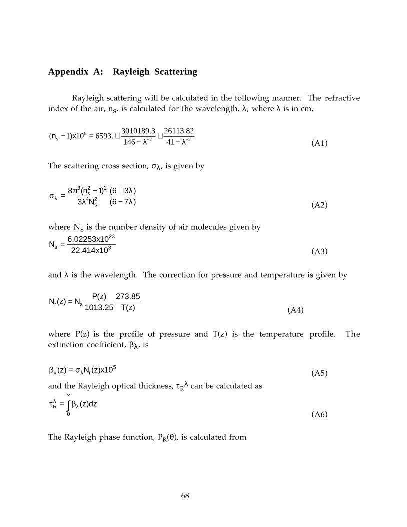
68

Appendix A: Rayleigh Scattering

Rayleigh scattering will be calculated in the following manner. The refractiveindex of the air, ns, is calculated for the wavelength, λ, where λ is in cm,

( ) .. .

n xs − = +−

+−− −1 10 6593

3010189 3146

26113 8241

82 2λ λ (A1)

The scattering cross section, σλ, is given by

σ πλ

λλλ = − +

−8 1

36 36 7

3 2 2

4 2( ) ( )

( )n

Ns

s (A2)

where Ns is the number density of air molecules given by

Nxxs = 6 02253 10

22 414 10

23

3.

. (A3)

and λ is the wavelength. The correction for pressure and temperature is given by

N z NP z

T zr s( )( )

..

( )=

1013 25273 85

(A4)

where P(z) is the profile of pressure and T(z) is the temperature profile. Theextinction coefficient, βλ , is

β σλ λ( ) ( )z N z xr= 105(A5)

and the Rayleigh optical thickness, τRλ can be calculated as

τ βλλR z dz=

∞

∫ ( )0 (A6)

The Rayleigh phase function, PR(θ), is calculated from

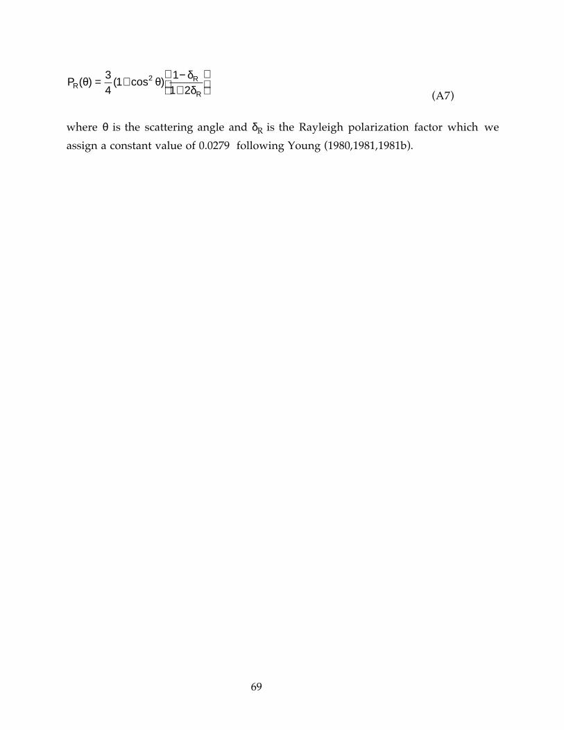
69

PRR

R

( ) ( cos )θ θ δδ

= + −+

34

11

1 22

(A7)

where θ is the scattering angle and δR is the Rayleigh polarization factor which we

assign a constant value of 0.0279 following Young (1980,1981,1981b).

70

Appendix B: Error Sensitivity study

Appendix B1) Top of the atmosphere signal (at 3 optical depths at550nm: 0.1,0.3,0.5) and sensitivity to error on optical depths (errorbars) for each cover type.

71

0.00

0.10

0.20

0.30

0.40

0.50

0.60

-80 -60 -40 -20 0 20 40 60 80

Broadleaf Crops


band5band6band7

Top

of

the

atm

osph

ere

Ref

lect

ance

θv

SUN

τa= 0 . 1


0.00

0.10

0.20

0.30

0.40

0.50

0.60

-80 -60 -40 -20 0 20 40 60 80

Broadleaf Crops

Su

rfa

ce

Re

flect

an

ce

θv

τa= 0 . 1±( 0 . 0 5 + 0 . 2τ

a)


SUN

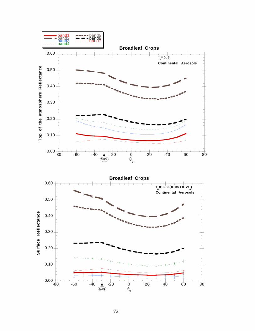
72

0.00

0.10

0.20

0.30

0.40

0.50

0.60

-80 -60 -40 -20 0 20 40 60 80

Broadleaf Crops


band5band6band7

Top

of

the

atm

osph

ere

Ref

lect

ance

θv

SUN

τa= 0 . 3


0.00

0.10

0.20

0.30

0.40

0.50

0.60

-80 -60 -40 -20 0 20 40 60 80

Broadleaf Crops

Su

rfa

ce

Re

flect

an

ce

θv

τa= 0 . 3±( 0 . 0 5 + 0 . 2τ

a)


SUN

73

0.00

0.10

0.20

0.30

0.40

0.50

-80 -60 -40 -20 0 20 40 60 80

Broadleaf Crops


band5band6band7

0.00

0.10

0.20

0.30

0.40

0.50

0.60

-80 -60 -40 -20 0 20 40 60 80

Broadleaf Crops

Sur

face

R

efle

ctan

ce

θv

τa= 0 . 5±( 0 . 0 5 + 0 . 2τ

a)


SUN

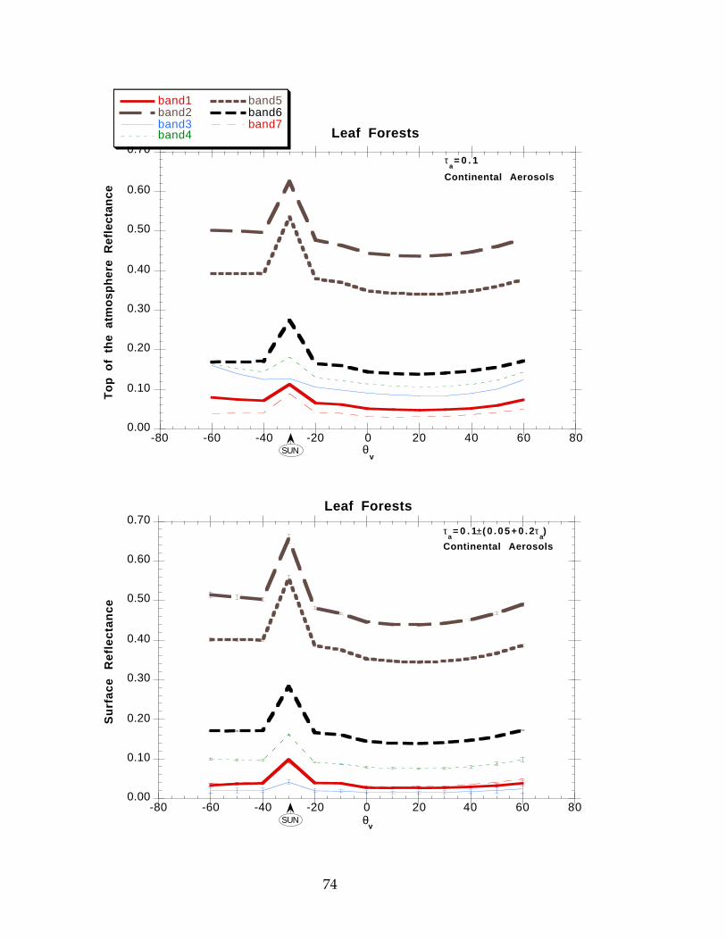
74

0.00

0.10

0.20

0.30

0.40

0.50

0.60

0.70

-80 -60 -40 -20 0 20 40 60 80

Leaf Forests


band5band6band7

Top

of

the

atm

osph

ere

Ref

lect

ance

θv

SUN

τa= 0 . 1


0.00

0.10

0.20

0.30

0.40

0.50

0.60

0.70

-80 -60 -40 -20 0 20 40 60 80

Leaf Forests

Su

rfa

ce

Re

flect

an

ce

θv

τa= 0 . 1±( 0 . 0 5 + 0 . 2τ

a)


SUN

75

0.00

0.10

0.20

0.30

0.40

0.50

0.60

-80 -60 -40 -20 0 20 40 60 80

Leaf Forests


band5band6band7

Top

of

the

atm

osph

ere

Ref

lect

ance

θv

SUN

τa= 0 . 3


0.00

0.10

0.20

0.30

0.40

0.50

0.60

0.70

-80 -60 -40 -20 0 20 40 60 80

Leaf Forests

Su

rfa

ce

Re

flect

an

ce

θv

τa= 0 . 3±( 0 . 0 5 + 0 . 2τ

a)


SUN

76

0.00

0.10

0.20

0.30

0.40

0.50

0.60

-80 -60 -40 -20 0 20 40 60 80

Leaf Forests


band5band6band7

Top

of

the

atm

osph

ere

Ref

lect

ance

θv

SUN

τa= 0 . 5


0.00

0.10

0.20

0.30

0.40

0.50

0.60

0.70

-80 -60 -40 -20 0 20 40 60 80

Leaf Forests

Su

rfa

ce

Re

flect

an

ce

θv

τa= 0 . 5±( 0 . 0 5 + 0 . 2τ

a)


SUN

77

0.00

0.10

0.20

0.30

0.40

0.50

0.60

0.70

-80 -60 -40 -20 0 20 40 60 80

Grasses/Cereal Crops


band5band6band7

Top

of

the

atm

osph

ere

Ref

lect

ance

θv

SUN

τa= 0 . 1


0.00

0.10

0.20

0.30

0.40

0.50

0.60

0.70

-80 -60 -40 -20 0 20 40 60 80


Su

rfa

ce

Re

flect

an

ce

θv

τa= 0 . 1±( 0 . 0 5 + 0 . 2τ

a)


SUN

78

0.00

0.10

0.20

0.30

0.40

0.50

0.60

0.70

-80 -60 -40 -20 0 20 40 60 80



band5band6band7

Top

of

the

atm

osph

ere

Ref

lect

ance

θv

SUN

τa= 0 . 3


0.00

0.10

0.20

0.30

0.40

0.50

0.60

0.70

-80 -60 -40 -20 0 20 40 60 80


Su

rfa

ce

Re

flect

an

ce

θv

τa= 0 . 3±( 0 . 0 5 + 0 . 2τ

a)


SUN

79

0.00

0.10

0.20

0.30

0.40

0.50

0.60

-80 -60 -40 -20 0 20 40 60 80



band5band6band7

Top

of

the

atm

osph

ere

Ref

lect

ance

θv

SUN

τa= 0 . 5


0.00

0.10

0.20

0.30

0.40

0.50

0.60

0.70

-80 -60 -40 -20 0 20 40 60 80


Sur

face

R

efle

ctan

ce

θv

τa= 0 . 5±( 0 . 0 5 + 0 . 2τ

a)


SUN

80

0.00

0.10

0.20

0.30

0.40

0.50

0.60

0.70

-80 -60 -40 -20 0 20 40 60 80

Needle Forests


band5band6band7

Top

of

the

atm

osph

ere

Ref

lect

ance

θv

SUN

τa= 0 . 1


0.00

0.10

0.20

0.30

0.40

0.50

0.60

0.70

-80 -60 -40 -20 0 20 40 60 80

Needle Forests

Su

rfa

ce

Re

flect

an

ce

θv

τa= 0 . 1±( 0 . 0 5 + 0 . 2τ

a)


SUN

81

0.00

0.10

0.20

0.30

0.40

0.50

0.60

-80 -60 -40 -20 0 20 40 60 80

Needle Forests


band5band6band7

Top

of

the

atm

osph

ere

Ref

lect

ance

θv

SUN

τa= 0 . 3


0.00

0.10

0.20

0.30

0.40

0.50

0.60

0.70

-80 -60 -40 -20 0 20 40 60 80

Needle Forests

Su

rfa

ce

Re

flect

an

ce

θv

τa= 0 . 3±( 0 . 0 5 + 0 . 2τ

a)


SUN

82

0.00

0.10

0.20

0.30

0.40

0.50

0.60

-80 -60 -40 -20 0 20 40 60 80

Needle Forests


band5band6band7

Top

of

the

atm

osph

ere

Ref

lect

ance

θv

SUN

τa= 0 . 5


0.00

0.10

0.20

0.30

0.40

0.50

0.60

0.70

-80 -60 -40 -20 0 20 40 60 80

Needle Forests

Su

rfa

ce

Re

flect

an

ce

θv

τa= 0 . 5±( 0 . 0 5 + 0 . 2τ

a)


SUN

83

0.00

0.10

0.20

0.30

0.40

0.50

0.60

0.70

-80 -60 -40 -20 0 20 40 60 80

Savanna


band5band6band7

Top

of

the

atm

osph

ere

Ref

lect

ance

θv

SUN

τa= 0 . 1


0.00

0.10

0.20

0.30

0.40

0.50

0.60

0.70

-80 -60 -40 -20 0 20 40 60 80

Savanna

Su

rfa

ce

Re

flect

an

ce

θv

τa= 0 . 1±( 0 . 0 5 + 0 . 2τ

a)


SUN

84

0.00

0.10

0.20

0.30

0.40

0.50

0.60

0.70

-80 -60 -40 -20 0 20 40 60 80

Savanna


band5band6band7

0.00

0.10

0.20

0.30

0.40

0.50

0.60

0.70

-80 -60 -40 -20 0 20 40 60 80

Savanna

Sur

face

R

efle

ctan

ce

θv

τa= 0 . 3±( 0 . 0 5 + 0 . 2τ

a)


SUN

85

0.10

0.20

0.30

0.40

0.50

0.60

-80 -60 -40 -20 0 20 40 60 80

Savanna


band5band6band7

Top

of

the

atm

osph

ere

Ref

lect

ance

θv

SUN

τa= 0 . 5


0.00

0.10

0.20

0.30

0.40

0.50

0.60

0.70

-80 -60 -40 -20 0 20 40 60 80

Savanna

Sur

face

R

efle

ctan

ce

θv

τa= 0 . 5±( 0 . 0 5 + 0 . 2τ

a)


SUN

86

0.00

0.20

0.40

0.60

0.80

1.00

-80 -60 -40 -20 0 20 40 60 80

Shrublands


band5band6band7

Top

of

the

atm

osph

ere

Ref

lect

ance

θv

SUN

τa= 0 . 1


87

0.00

0.20

0.40

0.60

0.80

1.00

-80 -60 -40 -20 0 20 40 60 80

ShrublandsS

urf

ace

R

efle

cta

nce

θv

τa= 0 . 1±( 0 . 0 5 + 0 . 2τ

a)


SUN

88

0.00

0.20

0.40

0.60

0.80

1.00

-80 -60 -40 -20 0 20 40 60 80

Shrublands


band5band6band7

Top

of

the

atm

osph

ere

Ref

lect

ance

θv

SUN

τa= 0 . 3


0.00

0.20

0.40

0.60

0.80

1.00

-80 -60 -40 -20 0 20 40 60 80

Shrublands

Su

rfa

ce

Re

flect

an

ce

θv

τa= 0 . 3±( 0 . 0 5 + 0 . 2τ

a)


SUN

89

0.00

0.20

0.40

0.60

0.80

1.00

-80 -60 -40 -20 0 20 40 60 80

Shrublands


band5band6band7

Top

of

the

atm

osph

ere

Ref

lect

ance

θv

SUN

τa= 0 . 5


0.00

0.20

0.40

0.60

0.80

1.00

-80 -60 -40 -20 0 20 40 60 80

Shrublands

Su

rfa

ce

Re

flect

an

ce

θv

τa= 0 . 5±( 0 . 0 5 + 0 . 2τ

a)


SUN

90

Appendix B2) ERRORS DUE TO CALIBRA TION UNCERTAINTIES(±2%) AT OPTICAL DEPTH AT 550nm of 0.3.

91

0.00

0.10

0.20

0.30

0.40

0.50

0.60

-80 -60 -40 -20 0 20 40 60 80

Broadleaf crops(calibration uncertainties)


band5band6band7

Su

rfa

ce

Re

flect

an

ce

θv

SUN

τa= 0 . 3


0.00

0.10

0.20

0.30

0.40

0.50

0.60

0.70

-80 -60 -40 -20 0 20 40 60 80

Grasses/Cereal Crops(calibration uncertainties)

Su

rfa

ce

Re

flect

an

ce

θv

SUN

τa= 0 . 3


92

0.00

0.10

0.20

0.30

0.40

0.50

0.60

0.70

-80 -60 -40 -20 0 20 40 60 80

Leaf Forests(calibration uncertainties)


band5band6band7

Su

rfa

ce

Re

flect

an

ce

θv

SUN

τa= 0 . 3


0.00

0.10

0.20

0.30

0.40

0.50

0.60

0.70

-80 -60 -40 -20 0 20 40 60 80

Needle Forests(calibration uncertainties)

Su

rfa

ce

Re

flect

an

ce

θv

SUN

τa= 0 . 3


93

0.00

0.10

0.20

0.30

0.40

0.50

0.60

0.70

-80 -60 -40 -20 0 20 40 60 80

Savanna(calibration uncertainties)


band5band6band7

Su

rfa

ce

Re

flect

an

ce

θv

SUN

τa= 0 . 3


0.00

0.20

0.40

0.60

0.80

1.00

-80 -60 -40 -20 0 20 40 60 80

Shrublands(calibration uncertainties)

Su

rfa

ce

Re

flect

an

ce

θv

SUN

τa= 0 . 3


94

Appendix B3) Errors due to aerosol model choice (at optical depthof 0.3 at 550nm).

The data were corrected with a continental aerosol model. The actual aerosol

model used to simulate top of the atmosphere reflectances was dust ( 6 S

background desertic model) or smoke (6S biomass burning model).

95

0.00

0.10

0.20

0.30

0.40

0.50

0.60

-80 -60 -40 -20 0 20 40 60 80

Broadleaf CropsError on aerosol model : Biomass Burning


band5band6band7

Su

rfa

ce

Re

flect

an

ce

θv

SUN

τa= 0 . 3


0.00

0.10

0.20

0.30

0.40

0.50

0.60

-80 -60 -40 -20 0 20 40 60 80

Broadleaf CropsError on aerosol model : Background Desertic

Su

rfa

ce

Re

flect

an

ce

θv

SUN

τa= 0 . 3


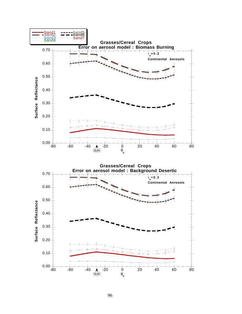
96

0.00

0.10

0.20

0.30

0.40

0.50

0.60

0.70

-80 -60 -40 -20 0 20 40 60 80

Grasses/Cereal CropsError on aerosol model : Biomass Burning


band5band6band7

Su

rfa

ce

Re

flect

an

ce

θv

SUN

τa= 0 . 3


0.00

0.10

0.20

0.30

0.40

0.50

0.60

0.70

-80 -60 -40 -20 0 20 40 60 80

Grasses/Cereal CropsError on aerosol model : Background Desertic

Su

rfa

ce

Re

flect

an

ce

θv

SUN

τa= 0 . 3


97

0.00

0.10

0.20

0.30

0.40

0.50

0.60

0.70

-80 -60 -40 -20 0 20 40 60 80

Leaf forestsError on aerosol model : Biomass Burning


band5band6band7

Su

rfa

ce

Re

flect

an

ce

θv

SUN

τa= 0 . 3


0.00

0.10

0.20

0.30

0.40

0.50

0.60

0.70

-80 -60 -40 -20 0 20 40 60 80

Leaf ForestsError on aerosol model : Background Desertic

Su

rfa

ce

Re

flect

an

ce

θv

SUN

τa= 0 . 3


98

0.00

0.10

0.20

0.30

0.40

0.50

0.60

0.70

-80 -60 -40 -20 0 20 40 60 80

Needle ForestsError on aerosol model : Biomass Burning


band5band6band7

Su

rfa

ce

Re

flect

an

ce

θv

SUN

τa= 0 . 3


0.00

0.10

0.20

0.30

0.40

0.50

0.60

0.70

-80 -60 -40 -20 0 20 40 60 80

Needle ForestsError on aerosol model : Background Desertic

Su

rfa

ce

Re

flect

an

ce

θv

SUN

τa= 0 . 3


99

0.00

0.10

0.20

0.30

0.40

0.50

0.60

0.70

-80 -60 -40 -20 0 20 40 60 80

SavannaError on aerosol model : Biomass Burning


band5band6band7

Su

rfa

ce

Re

flect

an

ce

θv

SUN

τa= 0 . 3


0.00

0.10

0.20

0.30

0.40

0.50

0.60

0.70

-80 -60 -40 -20 0 20 40 60 80

SavannaError on aerosol model : Background Desertic

Su

rfa

ce

Re

flect

an

ce

θv

SUN

τa= 0 . 3


100

0.00

0.20

0.40

0.60

0.80

1.00

-80 -60 -40 -20 0 20 40 60 80

ShrublandsError on aerosol model : Biomass Burning


band5band6band7

Su

rfa

ce

Re

flect

an

ce

θv

SUN

τa= 0 . 3


0.00

0.20

0.40

0.60

0.80

1.00

-80 -60 -40 -20 0 20 40 60 80

ShrublandsError on aerosol model : Background Desertic

Su

rfa

ce

Re

flect

an

ce

θv

SUN

τa= 0 . 3


101

Appendix B4) Error due to BRDF atmosphere coupling (at optical o f0.3 at 550nm).

The error when using the lambertian assumption is presented (symbols) .The

error bars are error estimate when using a generic BRDF and equations 15,16a-c

for correction. Broadleaf and savanna BRDF are used for correcting grassland,

leaf forest BRDF is used for correcting shrubland.

102

0.00

0.10

0.20

0.30

0.40

0.50

0.60

0.70

-80 -60 -40 -20 0 20 40 60 80

Grasses/Cereal Crops : BRDF couplinglambertian assumption



ρ7 lambρ1ρ2

ρ3ρ4ρ5

ρ6ρ7

Srf

ace

Ref

lect

ance

θv

τa= 0 . 3


0.00

0.10

0.20

0.30

0.40

0.50

0.60

0.70

-80 -60 -40 -20 0 20 40 60 80

Srf

ace

Ref

lect

ance

θv

τa= 0 . 3


Grasses/Cereal Crops Corrected using Broadleaf BRDF

103

0.00

0.10

0.20

0.30

0.40

0.50

0.60

0.70

-80 -60 -40 -20 0 20 40 60 80

Grasses/Cereal Crops corrected using savanna BRDFS

urfa

ce

Ref

lect

ance

θv

τa= 0 . 3


0.00

0.20

0.40

0.60

0.80

1.00

-80 -60 -40 -20 0 20 40 60 80

Shrublands: BRDF coupling lambertian assumption



ρ7 lambρ1ρ2

ρ3ρ4ρ5

ρ6ρ7

Sur

face

R

efle

ctan

ce

θv

τa= 0 . 3


104

0.00

0.20

0.40

0.60

0.80

1.00

-80 -60 -40 -20 0 20 40 60 80

Sur

face

R

efle

ctan

ce

θv

τa= 0 . 3


Shrubland corrected using leaf forest BRDF

105

Appendix C answers to the SWAMP 96 land product review.

Recommendation 3 Consolidate atmospheric scattering (correction) models

Several atmospheric scattering models are being used by various investigatorswithin one instrument team and across-instrument teams. The main rationalegiven in using one rather than another approach is familiarity and impliedconfidence. However, it is possible that the atmospherically-corrected data based onone model may be different than from another model, leading to different resultswhen corrected data is used. Also, cross-comparisons or joint use of similar orcomplementary products from various sensors may be thwarted. It is recommendedthat various atmospheric scattering investigators establish formal collaboration tocompare and contrast different models to come to closure on this issue. It is ourfeeling that, at a minimum all the models use similar physical assumptions andhave similar sensitivity to errors (it is realized that the technique used in solvingappropriate equations may have to be different), such that corrections are consistent.If physically different models have to be used, a conversion table (if feasible) for onemodel against another will be desirable for the users.

-> The model we are using (6S) is available to the general community and has been

compared to other scattering models. The EOS-AM1 atmospheric correction

(Martonchik,Thome,Vermote:Chair) group plans to point out differences in the

MISR/ASTER/MODIS approaches and compare the different models.

(a) technical/scientific soundness of the algorithm/approach described

(Rating: 6)The algorithm is similar in spirit to those used by ASTER and MISR teams. Themain questions are accuracy and uncertainty of the results (ATBD does not present aserious error analysis) and the size of the LUT table vs. fineness of the parametergrid (a finer grid will increase the size but ensure a more accurate retrieval). Notethat the accuracy of the approach depends on the accuracy of the input parameters.Two of these parameters -- aerosol optical thickness and BRDF are themselvesproducts of MODIS and/or MISR algorithms.

106

Since the MISR and ASTER teams are working on the same problem (althoughspatial resolutions are different), a collaboration with those team members will bebeneficial. It is recognized that various atmospheric scattering models are being usedby various investigators within one instrument team and across-instrument teams.

-> We try to improve on error analysis (appendix B of ATBD), error analysis shows that the

LUT resolution is sufficient (error <0.001 reflectance unit). We recognize the value of

working with other teams for the atmospheric correction and are going to embrace this

recommendation by working out common issues in the EOS-AM1 atmospheric correction

group.

(b) value of the data product to the Land science community (Rating: 6)The data on spectral reflectances will obviously be useful, provided it is accurate. Inthe absence of error analysis, (see comments under technical/scientific soundness),it is difficult to properly assess the value of the product.

-> We are now addressing error analysis (see appendix B of the ATBD).

(c) soundness of the validation strategy (Rating: 5)The atmospheric correction scheme will be validated using sun photometer datacollected at a series of test sites with known land cover characteristics in conjunctionwith data from existing sensor systems (AVHRR, AVIRIS, TM, MAS), includingSCAR-A data set intercomparison. The surface reflectance product will be validatedusing a combination of ground-based measurements, airborne measurements,comparison with other sensor data and image analysis.

The details of the validation approach are not given.

-> There is now more details for validation planning, both in the ATBD and in the

MODLAND validation plan.

(e) near-term recommendations for improvements to the data product

¥ It is recommended that a formal collaboration be established between MODIS,ASTER and MISR teams to compare and contrast various algorithms. This should

107

lead to cross-fertilization of ideas with respect to the accuracy and efficiency of thealgorithm(s) adopted.

-> see (a),(b)

(f) long-term recommendations for improvements or additions to the data

product

¥ Atmospheric correction formal collaborations between MODIS, ASTER and MISRteams as recommended above would be expected to determine which of themodel/algorithm (physical assumptions and mathematical approach) approachesare likely to give best surface reflectance and surface radiance.

¥ Likewise, the issues (described previously) regarding accuracy, speed, grid size,input parameters, and methodologies associated with the use of a look-up table(LUT) for model inversion could be investigated jointly.

-> see (a),(b)

==

MODIS Algorithm Technical Background Document …Distribution Function (BRDF) and atmosphere...

Documents

Transcript of MODIS Algorithm Technical Background Document …Distribution Function (BRDF) and atmosphere...