MODIS BRDF Albedo Product: Algorithm Theoretical Basis ...
252
-
Upload
truongliem -
Category
Documents
-
view
232 -
download
0
Transcript of MODIS BRDF Albedo Product: Algorithm Theoretical Basis ...

MODIS BRDF/Albedo Product:
Algorithm Theoretical Basis DocumentVersion 4.0
Principal Investigators:
A. H. Strahler, J.-P. Muller, MODIS Science Team Members
Document Prepared by
Alan H. Strahler1, Wolfgang Wanner1, Crystal Barker Schaaf1,
Xiaowen Li1;3, Baoxin Hu1;3,
Jan-Peter Muller2, Philip Lewis2, Michael J. Barnsley4
1 Boston University2 University College London
3 Institute of Remote Sensing Application, Chinese Academy of Sciences4 University of Wales, Swansea
MODIS Product ID: MOD43
Version 4.0 { November 1996
2
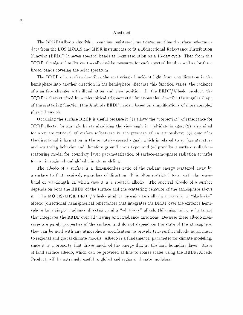
Abstract
The BRDF/Albedo algorithm combines registered, multidate, multiband surface re ectance
data from the EOS MODIS and MISR instruments to �t a Bidirectional Re ectance Distribution
Function (BRDF) in seven spectral bands at 1-km resolution on a 16-day cycle. Then from this
BRDF, the algorithm derives two albedo-like measures for each spectral band as well as for three
broad bands covering the solar spectrum.
The BRDF of a surface describes the scattering of incident light from one direction in the
hemisphere into another direction in the hemisphere. Because this function varies, the radiance
of a surface changes with illumination and view position. In the BRDF/Albedo product, the
BRDF is characterized by semiempirical trigonometric functions that describe the angular shape
of the scattering function (the Ambrals BRDF model) based on simpli�cations of more complex
physical models.
Obtaining the surface BRDF is useful because it (1) allows the \correction" of re ectance for
BRDF e�ects, for example by standardizing the view angle in multidate images; (2) is required
for accurate retrieval of surface re ectance in the presence of an atmosphere; (3) quanti�es
the directional information in the remotely- sensed signal, which is related to surface structure
and scattering behavior and therefore ground cover type; and (4) provides a surface radiation-
scattering model for boundary layer parameterization of surface-atmosphere radiation transfer
for use in regional and global climate modeling.
The albedo of a surface is a dimensionless ratio of the radiant energy scattered away by
a surface to that received, regardless of direction. It is often restricted to a particular wave-
band or wavelength, in which case it is a spectral albedo. The spectral albedo of a surface
depends on both the BRDF of the surface and the scattering behavior of the atmosphere above
it. The MODIS/MISR BRDF/Albedo product provides two albedo measures: a \black-sky"
albedo (directional{hemispherical re ectance) that integrates the BRDF over the exitance hemi-
sphere for a single irradiance direction, and a \white-sky" albedo (bihemispherical re ectance)
that integrates the BRDF over all viewing and irradiance directions. Because these albedo mea-
sures are purely properties of the surface, and do not depend on the state of the atmosphere,
they can be used with any atmospheric speci�cation to provide true surface albedo as an input
to regional and global climate models. Albedo is a fundamental parameter for climate modeling,
since it is a property that drives much of the energy ux at the land boundary layer. Maps
of land surface albedo, which can be provided at �ne to coarse scales using the BRDF/Albedo
Product, will be extremely useful to global and regional climate modelers.

CONTENTS 3
Contents
1 INTRODUCTION 6
1.1 ALGORITHM AND DATA PRODUCT IDENTIFICATION : : : : : : : : : : : : : : : : : : 6
1.2 INTRODUCTION : : : : : : : : : : : : : : : : : : : : : : : : : : : : : : : : : : : : : : : : : : 6
1.3 DATA PRODUCT DESCRIPTION : : : : : : : : : : : : : : : : : : : : : : : : : : : : : : : : 7
1.4 DOCUMENT SCOPE : : : : : : : : : : : : : : : : : : : : : : : : : : : : : : : : : : : : : : : : 8
1.5 LIST OF APPLICABLE DOCUMENTS AND PUBLICATIONS : : : : : : : : : : : : : : : : 10
2 OVERVIEW AND BACKGROUND INFORMATION 14
2.1 INTRODUCTION : : : : : : : : : : : : : : : : : : : : : : : : : : : : : : : : : : : : : : : : : : 14
2.2 MODELING OVERVIEW : : : : : : : : : : : : : : : : : : : : : : : : : : : : : : : : : : : : : : 15
2.3 EOS CONTEXT : : : : : : : : : : : : : : : : : : : : : : : : : : : : : : : : : : : : : : : : : : : 17
2.4 EXPERIMENTAL OBJECTIVE : : : : : : : : : : : : : : : : : : : : : : : : : : : : : : : : : : 18
2.5 HISTORICAL PERSPECTIVE : : : : : : : : : : : : : : : : : : : : : : : : : : : : : : : : : : : 19
2.6 INSTRUMENT CHARACTERISTICS OF MODIS AND MISR : : : : : : : : : : : : : : : : : 20
2.6.1 Spectral Characteristics : : : : : : : : : : : : : : : : : : : : : : : : : : : : : : : : : : : 20
2.6.2 Directional Sampling : : : : : : : : : : : : : : : : : : : : : : : : : : : : : : : : : : : : : 21
2.6.3 Spatial Resolution : : : : : : : : : : : : : : : : : : : : : : : : : : : : : : : : : : : : : : 24
3 ALGORITHM DESCRIPTION 25
3.1 THEORETICAL DESCRIPTION : : : : : : : : : : : : : : : : : : : : : : : : : : : : : : : : : 25
3.1.1 Kernels : : : : : : : : : : : : : : : : : : : : : : : : : : : : : : : : : : : : : : : : : : : : 25
3.1.2 Kernel-Driven Models : : : : : : : : : : : : : : : : : : : : : : : : : : : : : : : : : : : : 29
3.1.3 The Modi�ed Walthall Model : : : : : : : : : : : : : : : : : : : : : : : : : : : : : : : 29
3.1.4 Advantages of Linear Models : : : : : : : : : : : : : : : : : : : : : : : : : : : : : : : : 29
3.1.5 Validation of Semiempirical Models : : : : : : : : : : : : : : : : : : : : : : : : : : : : 30
3.1.5.1 Fit of Semiempirical Models to Ground Data : : : : : : : : : : : : : : : : : : 30
3.1.5.2 Inversion and Fitting of Semiempirical Models to ASAS Data : : : : : : : : : 32
3.1.5.3 Inversion and Fitting of Semiempirical Models to AVHRR Data : : : : : : : 33
3.2 THE MODIS BRDF/ALBEDO ALGORITHM : : : : : : : : : : : : : : : : : : : : : : : : : : 34
3.2.1 Model Inversion and Retrieval of BRDF and Albedo : : : : : : : : : : : : : : : : : : : 34
3.2.1.1 Theoretical Background: Inversion : : : : : : : : : : : : : : : : : : : : : : : : 34
3.2.1.2 Advantages of the Kernel-Based Approach : : : : : : : : : : : : : : : : : : : 36
3.2.1.3 Matrix Inversion and Error Function Used : : : : : : : : : : : : : : : : : : : 36
3.2.1.4 Model Selection : : : : : : : : : : : : : : : : : : : : : : : : : : : : : : : : : : 37
3.2.1.5 Albedo Calculation : : : : : : : : : : : : : : : : : : : : : : : : : : : : : : : : 38
3.2.1.6 Algorithm Flow and Execution : : : : : : : : : : : : : : : : : : : : : : : : : : 38

4 CONTENTS
3.2.1.7 Quarter Degree Climate Model Grid : : : : : : : : : : : : : : : : : : : : : : : 39
3.2.2 The Algorithm for BRDF Retrieval by the Product User : : : : : : : : : : : : : : : : : 41
3.2.3 Narrowband to Broadband Albedo Conversion : : : : : : : : : : : : : : : : : : : : : : 41
3.2.4 The BRDF-Atmospheric Correction Loop : : : : : : : : : : : : : : : : : : : : : : : : : 42
3.2.5 Water Surfaces and Snow-Covered Surfaces : : : : : : : : : : : : : : : : : : : : : : : : 44
3.2.6 Topographic Correction : : : : : : : : : : : : : : : : : : : : : : : : : : : : : : : : : : : 44
3.3 PRACTICAL CONSIDERATIONS : : : : : : : : : : : : : : : : : : : : : : : : : : : : : : : : : 45
3.3.1 Cloud Cover : : : : : : : : : : : : : : : : : : : : : : : : : : : : : : : : : : : : : : : : : 45
3.3.2 Errors and Sensitivity : : : : : : : : : : : : : : : : : : : : : : : : : : : : : : : : : : : : 47
3.3.2.1 Retrieval Accuracies of BRDF and Albedo from MODIS and MISR Angular
Sampling : : : : : : : : : : : : : : : : : : : : : : : : : : : : : : : : : : : : : : 50
3.3.2.2 Sensitivity of MODIS and MISR BRDF and Albedo Retrieval to Noisy Data 53
3.3.3 Numerical Computation Considerations : : : : : : : : : : : : : : : : : : : : : : : : : : 56
3.3.4 Calibration and Validation : : : : : : : : : : : : : : : : : : : : : : : : : : : : : : : : : 56
3.3.4.1 Validation of Model Fit. : : : : : : : : : : : : : : : : : : : : : : : : : : : : : : 57
3.3.4.2 Large-Area Application : : : : : : : : : : : : : : : : : : : : : : : : : : : : : : 60
3.3.4.3 Postlaunch Validation : : : : : : : : : : : : : : : : : : : : : : : : : : : : : : : 61
3.3.5 Quality Control and Diagnostics : : : : : : : : : : : : : : : : : : : : : : : : : : : : : : 62
3.3.6 Exception Handling : : : : : : : : : : : : : : : : : : : : : : : : : : : : : : : : : : : : : 63
3.3.7 Data Dependencies : : : : : : : : : : : : : : : : : : : : : : : : : : : : : : : : : : : : : 65
3.3.8 Output Products : : : : : : : : : : : : : : : : : : : : : : : : : : : : : : : : : : : : : : 65
4 CONSTRAINTS, LIMITATIONS, ASSUMPTIONS 65
4.0.9 ASSUMPTIONS AND CONSTRAINTS : : : : : : : : : : : : : : : : : : : : : : : : : : 65
4.0.10 LIMITATIONS : : : : : : : : : : : : : : : : : : : : : : : : : : : : : : : : : : : : : : : : 66
ACKNOWLEDGEMENTS 66
5 LITERATURE CITED 67
6 RESPONSE TO ATBD REVIEWS 75
6.1 1994 REVIEW: Comments and Response : : : : : : : : : : : : : : : : : : : : : : : : : : : : : 75
6.1.1 Comments from the Reviewers (June, 1994) : : : : : : : : : : : : : : : : : : : : : : : : 75
6.1.2 Algorithm Changes in Response to the 1994 Review : : : : : : : : : : : : : : : : : : : 77
6.1.3 Speci�c Responses to the Panel's Comments : : : : : : : : : : : : : : : : : : : : : : : 78
6.1.4 Speci�c Responses to the Mail Reviewers' Comments : : : : : : : : : : : : : : : : : : : 80
6.1.5 Literature Cited : : : : : : : : : : : : : : : : : : : : : : : : : : : : : : : : : : : : : : : 85
6.2 1996 EOS LAND REVIEW: Comments and Response : : : : : : : : : : : : : : : : : : : : : : 86
CONTENTS 5
6.2.1 Comments from the Reviewers (Sept, 1996) : : : : : : : : : : : : : : : : : : : : : : : : 86
6.2.2 Speci�c Responses to the Land Review Panel's Comments (Section 5.2.6a of the EOS-
AM-1 Land Data Product Review Report) : : : : : : : : : : : : : : : : : : : : : : : : 89
APPENDIXA: VALIDATION OF KERNEL-DRIVEN SEMIEMPIRICALMODELS FOR
GLOBAL MODELING OF BIDIRECTIONAL REFLECTANCE (PAPER BY HU ET
AL.) 96
APPENDIX B: RETRIEVAL ACCURACIES OF BRDF AND ALBEDO FROM EOS-
MODIS AND MISR ANGULAR SAMPLING (PAPER BY WANNER) 117
APPENDIX C: NOISE SENSITIVITY OF BRDF AND ALBEDO RETRIEVAL FROM
THE EOS-MODIS AND MISR SENSORS WITH RESPECT TO ANGULAR SAM-
PLING (PAPER BY LEWIS AND WANNER) 138
APPENDIXD: THE SENSITIVITYOF ATMOSPHERIC CORRECTION OF REFLECTANCES
TO THE SURFACE BRDF (PAPER BY HU, WANNER AND STRAHLER) 152
APPENDIX E: GLOBAL RETRIEVAL OF BIDIRECTIONAL REFLECTANCE AND
ALBEDO OVER LAND FROM EOS MODIS AND MISR DATA: THEORY AND AL-
GORITHM (PAPER BY WANNER ET AL., JGR, 1997) 173
APPENDIX F: ASAS SCALING EXPERIMENTS FOR BRDF MODEL INVERSION
(SUMMARY OF A PAPER BY MULLER AND DISNEY) 201
APPENDIX G: LANDSAT-TM SPECTRAL ALBEDO EXTRACTION (SUMMARY OF
A PAPER BY DISNEY, MULLER ET AL.) 219
APPENDIX H: MONTE CARLO-RAY TRACING SIMULATIONS OF ASAS (SUM-
MARY OF A PAPER BY MULLER, DISNEY AND LEWIS) 224
APPENDIX I: MONITORING LAND SURFACE DYNAMICS IN THE HAPEX-SAHEL
AREA USING KERNEL-DRIVEN BRDF MODELS AND AVHRR DATA (SUM-
MARY OF A PAPER BY RUIZ DE LOPE AND LEWIS) 229
APPENDIX J: ESTIMATING LAND SURFACE ALBEDO IN THE HAPEX-SAHEL
SOUTHERN SUPER-SITE: INVERSION OF TWO BRDF MODELS AGAINSTMUL-
TIPLE ANGLE ASAS IMAGES (SUMMARY OF A PAPER BY BARNSLEY ET AL.)244

6 1 INTRODUCTION
MODIS BRDF/Albedo Product:
Algorithm Theoretical Basis DocumentVersion 4.0 { MOD43
1 INTRODUCTION
1.1 ALGORITHM AND DATA PRODUCT IDENTIFICATION
At-Launch:
� MOD43, Surface Re ectance; Parameter 3669, Bidirectional Re ectance
� MOD43, Surface Re ectance; Parameter 4332, Albedo
Post-Launch:
� MOD43, Surface Re ectance, Parameter 3665, Bidirectional Re ectance, with Topographic Correction
� MOD43, Surface Re ectance, Parameter 4333, Albedo, with Topographic Correction
1.2 INTRODUCTION
The earth's surface scatters radiation anisotropically in many wavelength regimes. The Bidirectional Re-
ectance Distribution Function (BRDF) speci�es the behavior of surface scattering as a function of illumina-
tion and view angles at a particular wavelength. The albedo of a surface describes the ratio of radiant energy
scattered upward and away from the surface in all directions to the downwelling irradiance incident upon the
surface. Like the BRDF, albedo is spectrally dependent. If the BRDF is known, the albedo can be derived
given knowledge of the atmospheric state. Note that the albedo is often integrated over all wavelengths of
the downwelling solar spectrum for applications involving surface energy balance, and the general use of
the term \albedo" implies this integration. However, in this document the term will also include spectral
albedo, depending on the context.
The anisotropic re ectance behavior of earth surfaces presents an important problem for the interpreta-
tion of remotely-sensed images. Because of this behavior, a re ectance value observed from a single angular
position cannot simply be multiplied by a constant to provide an albedo. Furthermore, since radiance mea-
surements of the same surface cover will vary with viewing position, incorrect scene inference can occur
when the same cover type is viewed under di�erent geometries or at di�erent times of day or season. On
the other hand, the anisotropic re ectance provides an opportunity to infer information about the physical
parameters of the surface cover that produce the anisotropic e�ect. Such inference will obviously require a
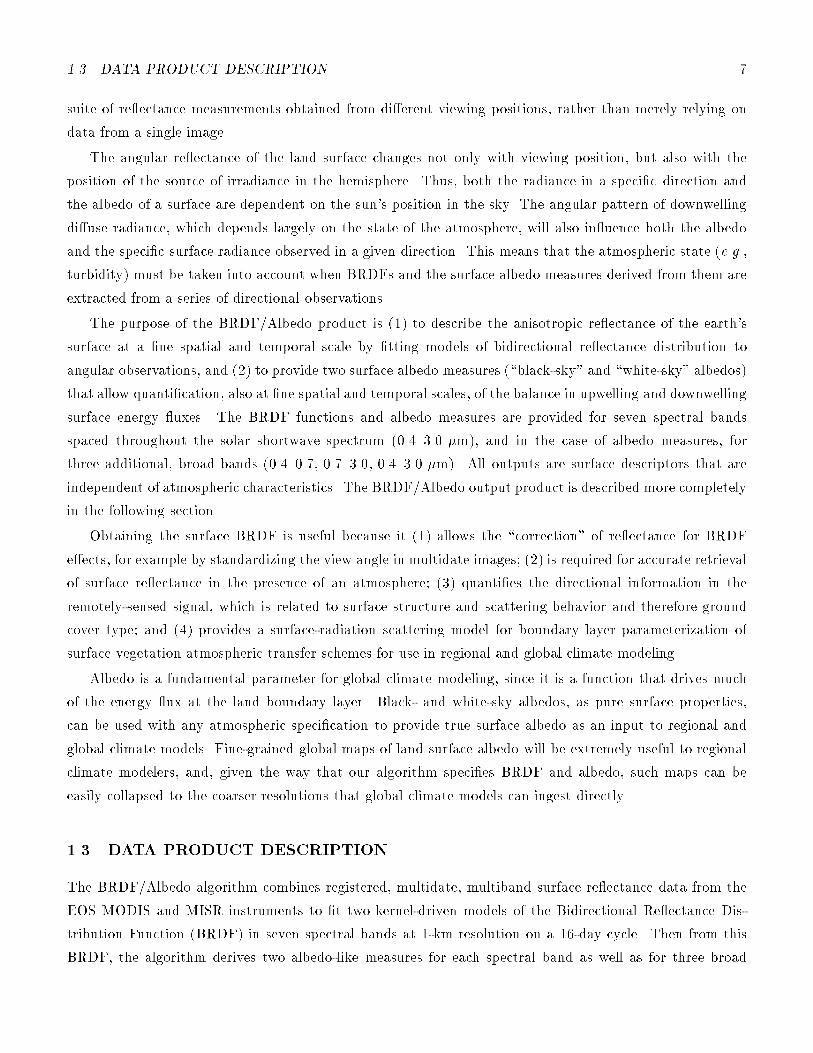
1.3 DATA PRODUCT DESCRIPTION 7
suite of re ectance measurements obtained from di�erent viewing positions, rather than merely relying on
data from a single image.
The angular re ectance of the land surface changes not only with viewing position, but also with the
position of the source of irradiance in the hemisphere. Thus, both the radiance in a speci�c direction and
the albedo of a surface are dependent on the sun's position in the sky. The angular pattern of downwelling
di�use radiance, which depends largely on the state of the atmosphere, will also in uence both the albedo
and the speci�c surface radiance observed in a given direction. This means that the atmospheric state (e.g.,
turbidity) must be taken into account when BRDFs and the surface albedo measures derived from them are
extracted from a series of directional observations.
The purpose of the BRDF/Albedo product is (1) to describe the anisotropic re ectance of the earth's
surface at a �ne spatial and temporal scale by �tting models of bidirectional re ectance distribution to
angular observations, and (2) to provide two surface albedo measures (\black-sky" and \white-sky" albedos)
that allow quanti�cation, also at �ne spatial and temporal scales, of the balance in upwelling and downwelling
surface energy uxes. The BRDF functions and albedo measures are provided for seven spectral bands
spaced throughout the solar shortwave spectrum (0.4{3.0 �m), and in the case of albedo measures, for
three additional, broad bands (0.4{0.7, 0.7{3.0, 0.4{3.0 �m). All outputs are surface descriptors that are
independent of atmospheric characteristics. The BRDF/Albedo output product is described more completely
in the following section.
Obtaining the surface BRDF is useful because it (1) allows the \correction" of re ectance for BRDF
e�ects, for example by standardizing the view angle in multidate images; (2) is required for accurate retrieval
of surface re ectance in the presence of an atmosphere; (3) quanti�es the directional information in the
remotely-sensed signal, which is related to surface structure and scattering behavior and therefore ground
cover type; and (4) provides a surface-radiation scattering model for boundary layer parameterization of
surface vegetation atmospheric transfer schemes for use in regional and global climate modeling.
Albedo is a fundamental parameter for global climate modeling, since it is a function that drives much
of the energy ux at the land boundary layer. Black- and white-sky albedos, as pure surface properties,
can be used with any atmospheric speci�cation to provide true surface albedo as an input to regional and
global climate models. Fine-grained global maps of land surface albedo will be extremely useful to regional
climate modelers, and, given the way that our algorithm speci�es BRDF and albedo, such maps can be
easily collapsed to the coarser resolutions that global climate models can ingest directly.
1.3 DATA PRODUCT DESCRIPTION
The BRDF/Albedo algorithm combines registered, multidate, multiband surface re ectance data from the
EOS MODIS and MISR instruments to �t two kernel-driven models of the Bidirectional Re ectance Dis-
tribution Function (BRDF) in seven spectral bands at 1-km resolution on a 16-day cycle. Then from this
BRDF, the algorithm derives two albedo-like measures for each spectral band as well as for three broad

8 1 INTRODUCTION
bands covering the solar spectrum. The gridded data are inverted using the kernel-driven semiempirical
Ambrals (Algorithm for MODIS bidirectional re ectance anisotropy of the land surface) BRDF model (us-
ing Ross-kernels, Li-kernels, and a specular kernel; see Wanner et al., 1995, 1997) and the empirical modi�ed
Walthall BRDF model (Walthall et al., 1995; Nilson and Kuusk, 1989), where the �rst consists of a weighted
sum of a volume-scattering (radiative transfer-based) kernel, a surface-scattering (geometric optics-based)
kernel, and a constant (isotropic contribution), the latter of a set of empirical kernels.
When su�cient and appropriate observations are available, the directional re ectance pattern of the land
surface element associated with each 1-km grid cell can be described by the kernels of the Ambrals BRDF
model used and corresponding kernel weights (parameters) that best represent the scattering involved. Thus,
the kernels producing the lowest root-mean-square (RMS) error in inversion of the observations are chosen
to describe the BRDF and derive the bihemispherical integral (\white-sky" albedo) and the directional-
hemispherical integral (\black-sky" albedo) of the BRDF. In addition, results from the empirical modi�ed
Walthall model are stored to allow global comparisons based on a single consistent model. The product will
be generated for all seven MODIS land bands; broadband albedos (0.4{0.7, 0.7{3.0, 0.4{3.0 �m) will also be
provided. The product will be derived over land only. Table 1 gives an overview of product contents.
Users of this product will be found among the global climate change community, most notably radiation
budget investigators, and among regional and mesoscale modelers. Further users include other AM-platform
teams, for example the MODIS atmospheric correction team or the CERES team, who will use surface
BRDF in cloud detection. The product will also be used in land cover classi�cation for the MODIS Land
Cover Product.
1.4 DOCUMENT SCOPE
In the remainder of this document, overview and background information will be provided �rst; this includes
the intended use of the BRDF products, and the history of the BRDF models. A detailed description of the
algorithm follows in Section 3. It is presented from both a theoretical and practical viewpoint and consists
of physical descriptions, mathematical formulations, uncertainty estimates, and discussions of various issues
arising in the actual numerical implementations. A brief discussion of the assumptions used in this algorithm
and various constraints is given in the �nal section.
Note that the development of the BRDF/Albedo algorithm is ongoing, and it will continue to be revised
and re�ned in both pre- and postlaunch phases. This document provides a snapshot of the algorithm valid
at the time of preparation of the document. Subsequent revisions will document the ongoing evolution of
the algorithm and supporting studies.

1.4 DOCUMENT SCOPE 9
Table 1: Outline of Contents of the MODIS BRDF/Albedo Product (Status: Version 1, 1996).
Param. Name Data Type Dimensions Comments
BRDF Model uint8 1: data rows Identi�es Ambrals BRDF model
Identi�er 2: data columns kernel combination and
3: number of output models (2) secondary global model used
BRDF Model int16 1: data rows BRDF model parameters will
Parameter 2: data columns allow reconstructing BRDF
3: number of output models (2) shape, white-sky albedo, and
4: number of land bands (7) black-sky albedo at any solar
5: number of model parameters (4) zenith angle
Albedo int16 1: data rows Albedo type 1 is white-sky albedo,
2: data columns albedo type 2 black-sky albedo
3: number of output models (2) at the mean sun angle of observation;
4: number of land bands + 3 (10) 3 extra bands contain broadband albedos
5: albedo type (2) for 0.4{0.7, 0.7{3.0 and 0.4{3.0 �m.
Quality Control uint8 1: data rows Flag information on overall quality
Flags 2: data columns (3 bits), data base of inversion
3: number of QC words (4) (5 bits), solar and viewing angle range
available (7 bits), extra QC data (7 bits)
Inversion uint16 1: data rows Lists: RMSE for the Ambrals model,
Information 2: data columns RMSE of the secondary uniform model,
3: number of words (6) sensitivity parameter, scattering type
indicator, BRDF type indicator, TBD;
the latter to be used for inferences.

10 1 INTRODUCTION
1.5 LIST OF APPLICABLE DOCUMENTS AND PUBLICATIONS
The following recent publications of the BRDF/Albedo team are especially relevant to the BRDF/Albedo
Product:
Abuelgasim, A. A. and A. H. Strahler, 1994, Modeling bidirectional radiance measurements collected by theAdvanced Solid-State Array Spectroradiometer (ASAS) over Oregon Transect conifer forests, RemoteSens. Environ. 47:261-275.
Abuelgasim, A.A., Gopal, S. and Strahler, A.H., 1996, Retrieval of canopy structural parameters frommultiangle observations using an arti�cial neural network, Proc. 1996 Internat. Geosci. Remote Sens.Symp., Lincoln, Neb., vol. 3, pp. 1426-1428.
Barnsley, M., Allison, D., and Lewis, P., 1995, On the Statistical Information Content of Multiple ViewAngle (MVA) Images. Proc. RSS 95, "Remote Sensing in Action", Southampton, UK, 11-14 Sept,1298-1305.
Barnsley, M., Disney, M., Lewis, P., Hesley, Z., and Muller, J-P. 1996, On the intrinsic dimensionality of theBRDF: Implications for the retrieval of land surface biophysical properties. Proc. RSS 96, Durham,UK. 69-70
Barnsley, M. J., and J.-P. Muller, 1991, Measurement, simulation and analysis of bidirectional re ectanceproperties of earth surface material, Proc. Int. Conf. Spectral Signatures in Remote Sens., Courchevel,France, January 14-18 1991, pp. 375-382.
Barnsley, M. J., A. H. Strahler, K. P. Morris, and J.-P. Muller, 1994, Sampling the surface bidirectionalre ectance distribution function (BRDF): Evaluation of current and future satellite sensors, RemoteSens. Rev. 8:271-311.
Burgess, D. W., Lewis, P., and Muller, J-P. 1995, Topographic E�ects in AVHRR NDVI Data. RemoteSens. Environ, 54, 223-232.
Boissard, P., Akkal, N., Lewis, P., 1996, 3D Plant Modelling in Agronomy. Association of Applied Biolo-gists: Modelling in Applied Biology: Spatial Aspects, 24/27 June 1996, Brunel, U.K.
Boissard, P., Akkal, N., Lewis, P., Valery, P., and Meynard, J-M., 1995, Linking a 3D Plant Model Databaseof Crop Structure to Models of Canopy Development. Int. Colloq. Photosynthesis and Remote Sensing,28-31 Aug. 1995, Montpellier, Fr.
d'Entremont, R.P., Schaaf, C.B., and Strahler, A., 1996, Cloud detection and land-surface albedos us-ing visible and near-infrared bidirectional re ectance distribution models, Proc. Amer. Met. Soc.Satellite. Met. Conf., January, 1996, Atlanta, GA, pp. 334-338.
d'Entremont, R.P., Schaaf, C.B., and Strahler, A.H., 1995, Cloud detection using visible and near-infraredbidirectional re ectance distribution models, Proc. CIDOS-95, (Cloud Impact on DOD Operationsand Systems), October 24-26, 1995, Hanscom AFB, MA, pp. 87-91.
Hesley, Z., Barnsley, M., and Lewis, P., 1996, The signi�cance of angular sampling errors of the MODISand MISR sensors on the retrieval of surface biophysical parameters from BRDF models. Proc. RSS96, Durham, UK. 537-542
1.5 LIST OF APPLICABLE DOCUMENTS AND PUBLICATIONS 11
Hesley, Z., Barnsley, M., and Lewis, P., 1995, E�ect of Angular Sampling Regimes on the Retrieval of Bio-physical Parameters from BRDF Models. Proc. RSS 95, "Remote Sensing in Action", Southampton,UK, 11-14 Sept, 342-349.
Hu, B., Li, X., and Strahler, A. H., 1996, Deriving the anisotropic point spread function of ASAS o�-nadirimages and removal of the adjacency e�ect, Proc. 1996 Internat. Geosci. Remote Sens. Symp.,Lincoln, Neb., May 27-31, vol. 3, pp. 1587-1589.
Hu, B., Wanner, W., Li, X., and Strahler, A.H., 1996, Validation of kernel-driven semiempirical models forapplication to MODIS/MISR data, Proc. 1996 Internat. Geosci. Remote Sens. Symp., Lincoln, Neb.,May 27-31, vol. 3, pp. 1669-1671.
Lewis, P., 1995, On the Implementation of Linear Kernel-Driven BRDF Models. Proc. RSS 95, "RemoteSensing in Action", Southampton, UK, 11-14 Sept, 333-340.
Lewis, P., 1995, The Utility of Linear Kernel-Driven BRDF Models in Global BRDF and Albedo Studies.Proc. 1995 Internat. Geosci. Remote Sens. Symp., Firenze, Italy, 1186{1188.
Lewis, P., and J.-P. Muller, 1992, The Advanced Radiometric Ray-Tracer: ARARAT for plant canopyre ectance simulation, Proc. 29th Cong. Int. Soc. Photogramm. Remote. Sens., Washington DC,pp. 26-34.
Lewis, P. and M. J. Barnsley, 1994, In uence of the sky radiance distribution on various formulations of theearth surface albedo, Proc. Sixth Int. Symp. on Physical Measurements and Signatures in RemoteSens., Val d'Isere, France, January 17-21 1994, pp. 707-715.
Lewis, P., Barnsley, M., Muller, J-P., and Sutherland, M., 1995, Deriving Spectral Albedo Maps forHAPEX-Sahel using Linear BRDF Models applied to ASAS and Landsat TM Data. Proc. 1995Internat. Geosci. Remote Sens. Symp., Firenze, Italy, 2221{2223.
Lewis, P., and Boissard, P., 1995, A Botanical Plant Modelling System: a Model for Deriving and DescribingPlant Form and Simulating the Canopy Shortwave Radiation Regime. Invited Paper (abstract only inproc.) RSS Meeting: "The Interaction of Vegetation Canopies with Radiation", She�eld CEOS, May24, 1995.
Li, X., and A. H. Strahler, 1986, Geometric-optical bidirectional re ectance modeling of a conifer forestcanopy, IEEE Trans. Geosci. Remote Sens. 24:906-919.
Li, X. and A. H. Strahler, 1992, Geometric-optical bidirectional re ectance modeling of the discrete-crownvegetation canopy: E�ect of crown shape and mutual shadowing, IEEE Trans. Geosci. Remote Sens.30:276-292.
Li, X., A. H. Strahler, and C. E. Woodcock, 1995, A hybrid geometric optical-radiative transfer approach formodeling albedo and directional re ectance of discontinuous canopies, IEEE Trans. Geosci. RemoteSens. 33: 466-480.
Li, X., and Strahler, A., 1996, A knowledge-based inversion of physical BRDF model and three examples,Proc. 1996 Internat. Geosci. Remote Sens. Symp., Lincoln, Neb., May 27-31, vol. 4, pp. 2173-2176.
Li, X., Ni, W., Woodcock, C.E., and Strahler, A.H., 1996, A simpli�ed hybrid model for radiation underdiscontinuous canopies, Proc. 1996 Internat. Geosci. Remote Sens. Symp., Lincoln, Neb., May 27-31,vol. 1, pp. 293-295.
12 1 INTRODUCTION
Li, X., and, Wang, J., 1995, Canopy Re ectance Models, Inversion, and Characterization of Canopy Struc-ture, Science Press, Beijing, 114 pp. (in Chinese).
Liang, S. and Lewis, P. 1996, A Parametric Radiative Transfer Model for Sky Radiance Distribution. J.Quant. Spectrosc. Radiat. Transfer, 55(2), 181-189.
Liang, S. and A. H. Strahler, 1993, An analytic BRDF model of canopy radiative transfer and its inversion,IEEE Trans. Geosci. Remote Sens. 31:1081-1092.
Liang, S. and A. H. Strahler, 1993, Calculation of the angular radiance distribution for a coupled systemof atmosphere and canopy media using an improved Gauss-Seidel algorithm, IEEE Trans. Geosci.Remote Sens. 31:491-502.
Liang, S. and A. H. Strahler, 1994, Retrieval of surface BRDF from multiangle remotely sensed data,Remote Sens. Environ. 50:18-30.
Liang, S. and A. H. Strahler, 1995, An analytic radiative transfer model for a coupled atmosphere and leafcanopy, J. Geophys. Res. 100:5085-5094.
Liang, S., and A. H. Strahler, 1993, An analytic BRDF model of canopy radiative transfer and its inversion,IEEE Trans. Geosci. Remote Sens. 31:1081-1092.
Liang, S., and A. H. Strahler, 1993, Retrieval of surface BRDF from multiangle remotely sensed data,Remote Sens. Environ. 50:18-30.
Liang, S., and A. H. Strahler, 1994, A four-stream solution for atmospheric radiance transfer over a non-Lambertian surface, Appl. Optics 33:5745-5753.
Newton, A., J.-P. Muller, and J. C. Pearson, 1991, SPOT-DEM shading and its application to automatedcorrection of topographic and atmospheric e�ects, Proc. Int. Geosci. Remote Sens. Symp., Espoo,Finland, June 3-6 1991, pp. 655- 659.
Ni, W., Li, X., Woodcock, C.E., Roujean, J.-L., Davis, R., and Strahler, A.H., 1996, Modeling solarradiation transmission in boreal conifer forests, Proc. 1996 Internat. Geosci. Remote Sens. Symp.,Lincoln, Neb., May 27-31, vol. 1, pp. 591-593.
Running, S., C. Justice, D. Hall, A. Huete, Y. Kaufman, J-P. Muller, A. Strahler, V. Vanderbilt, Z-M.Wan, P. Teillet and D. Carnegie, 1994, Terrestrial remote sensing science and algorithms planned forEOS/MODIS, Int. J. Remote Sens. 15:3587-3620.
Schaaf, C. B. and A. H. Strahler, 1993, Solar zenith angle e�ects on forest canopy hemispherical re ectancescalculated with a geometric-optical bidirectional re ectance model, IEEE Trans. Geosci. Remote Sens.31:921- 927.
Schaaf, C. B. and A. H. Strahler, 1994, Validation of bidirectional and hemispherical re ectances froma geometric-optical model using ASAS imagery and pyranometer measurements of a spruce forest,Remote Sens. Environ. 49:138-144.
Schaaf, C. B., X. Li and A. H. Strahler, 1994, Topographic e�ects of bidirectional and hemisphericalre ectances calculated with a geometric-optical canopy model, IEEE Trans. Geosci. Remote Sens.32:1186-1193.

1.5 LIST OF APPLICABLE DOCUMENTS AND PUBLICATIONS 13
So�er, R., Miller, J., Wanner, W., and Strahler, A.H., 1995, Winter boreal forest canopy BRF results:Comparisons between airborne data, laboratory simulations and geometrical-optical model data, Proc.1995 Internat. Geosci. Remote Sens. Symp., Florence, Italy, July 10-14, 1995, vol 1., pp. 800-802.
Sutherland, M., Barnsley, M., Lewis, P., and Muller, J-P., 1995, Derivation of Surface Biophysical Pa-rameters through Inversion of a BRDF Model for HAPEX-Sahel. Proc. RSS 95, "Remote Sensing inAction", Southampton, UK, 11-14 Sept, 325-332.
Strahler, A.H., Wanner, W., Zhu, Q., and Jin. X., 1995, Bidirectional re ectance modeling of data fromvegetation obtained in the Changchun solar simulation laboratory, Proc. 1995 Internat. Geosci.Remote Sens. Symp., Florence, Italy, July 10-14, 1995, vol. 3, pp. 1965-1967.
Strahler, A.H., 1996, An overview of MODIS products for land applications, Proc. 8th Australasian RemoteSens. Conf., Canberra, Australia, March 25-29, CD-ROM, 8 pp.
Strahler, A.H., 1996, AVHRR applications in support of MODIS product development, Proc. 8th Aus-tralasian Remote Sens. Conf., Canberra, Australia, March 25-29, CD-ROM, 4 pp.
Wang, J., Li, X., Strahler, A., 1995, Tree tomography-an indirect method for measuring crown structure,Proc. of GeoInfomatics'95, Hongkong, vol. 1, pp. 371-378.
Wanner, W., Li, X. Strahler, A.H., 1995, A new class of geometric-optical semiempirical kernels for globalBRDF and albedo modeling, Proc. 1995 Internat. Geosci. Remote Sens. Symp., Florence, Italy, July10-14, 1995, vol. 1, pp. 15-17.
Wanner, W., Strahler, A.H., Muller, J.P., Barnsley, M., Lewis, P., Li, X., and Schaaf, C.B., 1995, Globalmapping of bidirectional re ectance and albedo for the EOS MODIS project: The algorithm and theproduct, Proc. 1995 Internat. Geosci. Remote Sens. Symp., Florence, Italy, July 10-14, 1995, vol. 1,pp. 525-529.
Wanner, W., Strahler, A., Zhang, B., and Lewis, P., 1996, Kilometer-scale global albedo from MODIS,Proc. 1996 Internat. Geosci. Remote Sens. Symp., Lincoln, Neb., May 27-31, vol. 3, pp. 1405-1407.
Wanner, W., X. Li and Strahler, A., 1995, On the derivation of kernels for kernel-driven models of bidirec-tional re ectance, J. Geophys. Res., vol. 100, pp. 21077-21089.
Wanner, W., J.-L., Lewis, P., and Roujean, J.-L., 1996, The in uence of directional sampling on bidi-rectional re ectance and albedo retrieval using kernel-driven models, Proc. 1996 Internat. Geosci.Remote Sens. Symp., Lincoln, Neb., May 27-31, vol. 3, pp. 1408-1410.
White, H.P., Miller, J.R., So�er, R., and Wanner, W., 1996, Semiempirical modelling of bidirectionalre ectance utilizing the MODIS BRDF/Albedo models, Proc. 1996 Internat. Geosci. Remote Sens.Symp., Lincoln, Neb., May 27-31, vol. 3, pp. 1411-1413.
14 2 OVERVIEW AND BACKGROUND INFORMATION
2 OVERVIEW AND BACKGROUND INFORMATION
2.1 INTRODUCTION
The BRDF of a surface describes the scattering of incident light from one direction in the hemisphere into
another direction in the hemisphere. It will generally vary as a function of wavelength. That is,
fr(�i; �i; �v; �v; �) =dLv(�i; �i; �v; �v;Ei; �)
dE(�i; �i; �); (1)
where fr(�i; �i; �v; �v; �) in units of sr�1 is the BRDF in waveband �; �i; �i; �v; �v are zenith and azimuth
angles of the direction of irradiance and viewing, respectively; E(�i; �i; �) is the parallel-beam irradiance from
the illumination direction in waveband �; and Lv(�i; �i; �v; �v;Ei; �) is the radiance in the view direction in
waveband � under the conditions of illumination (Nicodemus et al., 1977).
In this document, we will de�ne the BRDF as � = � fr , so that the BRDF is directly comparable
with the bidirectional surface re ectance values and hemispherical-directional re ectance factors that the
BRDF/Albedo algorithm receives as inputs from other MODIS and MISR products. We will further use
the notation � to refer to true, parametric values of the BRDF; R to refer to modeled values of �; and
�0 to refer to observations of BRDF, normally obtained from top-of-atmosphere radiances as corrected for
atmospheric e�ects and surface BRDF. We will also assume the BRDF to be symmetric with respect to the
principal plane of the illumination direction, and thus expressed as a function of �i; �v; �, where � is the
relative azimuth between illumination and view directions, i.e. � = j�v � �ij,The BRDFs of land covers are known to show peaks in the function in the backward{scattering direction
of the principal plane, due to shadow hiding (e.g., Li and Strahler, 1986). This position in the viewing
hemisphere is known as the hotspot (Gerstl and Zardecki, 1985a, b), and its shape is characteristic of the
shape and density of surface projections (e.g., plant crowns) or scattering elements (e.g., leaves) of the
cover type (Jupp and Strahler, 1993). For some covers, notably water or wetlands, there will also be a
forward-scattering specular peak in the function.
The spectral albedo of a surface is a dimensionless ratio of the radiant energy scattered away from the
surface to that received by the surface at a particular waveband. That is,
�(�) =E"(�)
E#(�)=
R2�0
R �=20
L"(�v; �v; �) sin�v cos �v d�v d�vR2�0
R �=20
L#(�i; �i; �) sin�i cos �i d�i d�i; (2)
where �(�) is the spectral albedo in waveband �; E"(�) is the upwelling radiant energy ux from the surface
in waveband �; E#(�) is the downwelling radiant energy ux in waveband �; L"(�v; �v; �) is the upwelling
radiance in direction �v ; �v in waveband �; and L#(�i; �i; �) is the downwelling radiance in direction �i; �i in
waveband �. Note that the downwelling energy ux includes both the solar beam and the di�use irradiance
that is scattered downward by the atmosphere. Albedo is normally measured by paired instruments with
hemispherical �elds of view that integrate upwelling and downwelling radiance.
Because upwelling radiance depends on both the angular distribution of downwelling irradiance as well
as the surface BRDF, surface albedo is dependent on the atmospheric state. It can change within minutes
2.2 MODELING OVERVIEW 15
as clouds come and go, or within hours as an air mass with di�erent optical properties invades the region.
Albedo will further change over the course of the day with the sun's path in the sky, even for constant
atmospheric and surface conditions.
Rather than depending in this way on the state of the atmosphere, the albedo measures provided by
the MODIS/MISR BRDF/Albedo product are purely properties of the surface. Two measures are provided.
The �rst is directional{hemispherical re ectance �b, a measure that integrates the BRDF over the exitance
hemisphere for a single irradiance direction, which is normally the position of the sun in the sky at a time
of interest. That is,
�b(�i; �) =2
�
Z �
0
Z �=2
0
�(�i; �v; �; �) sin�v cos �v d�v d�; (3)
where �(�i; �v; �; �) is the BRDF in waveband �. Because the measure is not integrated over the sky
hemisphere for illumination directions, we refer to it as the \black-sky" albedo.
The second albedo measure is bihemispherical re ectance �w, which is the double integral in waveband
� of the BRDF over all viewing and irradiance positions. That is,
�w(�) = 2Z �=2
0
�b(�i; �) sin �i cos �i d�i: (4)
Since this integral weights all irradiance positions equally, it provides the albedo under conditions of perfectly
di�use illumination. Thus, we term it the \white-sky" albedo. Black-sky and white-sky albedos are provided
for each of the MODIS land bands as well as three broad bands covering the wavelength intervals 0.4{0.7 �m,
0.7{3.0 �m, and 0.4{3.0 �m. Broadband values are obtained by combining narrow-band measurements
weighted by standardized solar spectral irradiance functions.
2.2 MODELING OVERVIEW
In modeling the BRDF of a surface, two contrasting approaches are possible | physical and empirical. In
the empirical approach, a function (e.g., a set of spherical harmonics) is �tted that describes the shape of the
BRDF based on the observations at hand. That is, the BRDF is modeled as an empirical function of viewing
and illumination angles and azimuths in the hemisphere. For accurate �tting, this approach requires many
observations at numerous combinations of viewing and illumination positions. Although simple and direct,
the method is not very practical for remote-sensing applications because the number of angular observations
of a surface typically acquired by a single remote sensing instrument will usually be small. Furthermore, the
coe�cients that �t empirical models cannot be readily interpreted in terms of scene or surface properties.
Instead, relationships must be obtained by further empirical studies, such as through correlation analyses.
In the physical approach, a scattering model is constructed that explains anisotropic surface scattering
using physical principles. By inversion, re ectance observations are used to infer the physical parameters
that drive the model. Once these are known, the BRDF may be determined for any view or illumination
position without recourse to further measurements. Moreover, the parameters typically have physical inter-
pretations in their own right that are of intrinsic interest beyond simply generating the BRDF. Note that
16 2 OVERVIEW AND BACKGROUND INFORMATION
these parameters may vary among di�erent physical models. A disadvantage of the physical approach is
that a large number of parameters (perhaps 6 to 12) may be required to drive the model. Further, numerical
inversion is normally required, which is computationally very intensive and not always robust.
A third approach, which we may term \semiempirical," combines physical and empirical approaches.
Here, the BRDF is modeled as a weighted sum of a few (typically two or three) trigonometric functions of
view zenith, illumination zenith, and relative azimuth angles that describe the shape of the BRDF. However,
these functions are derived from physical approximations, and so have some physical meaning. The weight
given to each function is determined empirically by �t to the observations. Thus, it is the weights of
the physically-based functions that are retrieved, not a set of physical parameters governing the surface
scattering.
The MODIS/MISR BRDF/Albedo product utilizes this hybrid approach, �tting a suite of semiempirical
models to each set of angular observations. Each model typically consists of three components: a volume-
scattering function, a geometric surface-scattering function, and a constant ( i.e., an isotropically-scattering
function). The functions are referred to as \kernels" | hence, the corresponding semiempirical models may
be called \kernel-driven." For the current work we employ two choices of volume-scattering kernels and
two choices of geometric surface-scattering kernels developed for this project. We also exercise the modi�ed
Walthall model (Walthall et al., 1985; Nilson and Kuusk, 1989) which supplies a purely empirical �t for each
pixel on the globe. Although this model rarely provides the best �t, it is a simple and consistent expression
and has been widely applied. (Further details are provided in Section 3.1) Semiempirical models also have
the advantage of being very rapidly invertible, due to their linear nature. Furthermore, albedo calculations
are greatly simpli�ed since the kernels need to be integrated only once, before operational processing begins.
Section 2.5 summarizes the historical development of physical, empirical, and semiempirical models in the
literature.
In the �tting of surface BRDF models using top-of-atmosphere observations, a problem arises from the
interaction between the anisotropic surface scattering and atmospheric scattering. In general, the e�ect of
atmospheric scattering on surface BRDF retrieval will tend to damp the BRDF, making it appear more
isotropic. Surface re ectance, when retrieved assuming an isotropic surface, will be underestimated in the
bright parts of the BRDF and overestimated in the dark parts. Thus, surface BRDF is required to esti-
mate bidirectional surface re ectance accurately, while BRDF �tting requires accurate surface bidirectional
re ectances. In other words, some form of surface-atmosphere coupling is needed. To provide this coupling
in deriving the BRDF/Albedo Product, atmospheric parameters are archived with each surface re ectance
measurement, and a looping iteration is carried out in which (1) a surface BRDF is �tted to initial estimates
of surface re ectances; (2) surface re ectances are rederived using this BRDF and the atmospheric parame-
ters associated with each initial re ectance; and (3) a new and �nal BRDF is then �tted. More details are
provided in Section 3.2.4.

2.3 EOS CONTEXT 17
2.3 EOS CONTEXT
The algorithm we describe in this document is targeted speci�cally to the remote sensing scenario presented
by the EOS-AM and -PM platforms, which will place three instruments in polar orbits that can be used
for BRDF/Albedo retrieval. Two of these will be MODIS instruments. A MODIS will orbit on each of
the AM and PM platforms, with nominal equatorial crossing times of 10:30 and 13:30, respectively. By
virtue of its wide scan (�55�), MODIS images the earth on a two-day repeat cycle, with a one-day or
more frequent repeat at higher latitudes greater than 30� due to orbital convergence. Thus, the same point
on the ground will be potentially visible to MODIS from a number of di�erent illumination and viewing
positions in the hemisphere during the span of a few days. The third instrument, MISR (Multiangle Imaging
SpectroRadiometer), will y on the EOS-AM platform. MISR has a unique design that allows it to image the
same point on the ground from nine along-track angles (Diner et al., 1989). However, its across-track �eld
of view is more restricted than that of MODIS, providing a 9-day one-look repeat cycle for global coverage
as well as a 16-day two-look cycle. Relevant characteristics of the MODIS and MISR instruments for the
inference of BRDF and albedo measures are discussed more fully in Section 2.6.
For calibration and validation of the BRDF/Albedo product in the post-launch time frame, CERES data
will also prove useful. This instrument measures top-of-atmosphere and surface radiation ux in short- and
longwave regions. It has a much larger �eld of view than either MODIS or MISR | 21 km at nadir | so
that albedo can be validated only for broad regions. However, CERES will be very helpful in developing and
maintaining the narrow-to-broadband spectral calibration that we will use to generalize short- and longwave
albedos from MODIS and MISR sensors. Geostationary data from the GOES-NEXT and METEOSAT series
of instruments may also prove useful for validating BRDF, in that multiangle measurements of radiance from
a single point are acquired in the course of a single day. Postlaunch validation is discussed more fully in
Section 3.3.4.3.
Another satellite instrument that will prove useful is POLDER (Polarization and Directionality of the
Earth's Re ectances), a push{broom, wide{�eld, multiband imaging radiometer/polarimeter. Relying on
an area detector array and a rotating �lter wheel, POLDER is much like a framing camera that acquires
overlapping images along the satellite ground track. Data are acquired in eight bands, of which three are
designed for land imaging, centered at 443, 665, and 865 nm. The ADEOS satellite on which POLDER
is mounted was successfully launched at 10.53 a.m. (JST) / 01:53 a.m. (UT) on August 17, 1996 from
the Tanegashima Space Centre in Japan. ADEOS orbits the Earth in a height of about 800 km with an
inclination of 98.6� in 100.8 minutes; it has a 10:41 a.m. local time descending node and a recurrence cycle
of 41 days.
The initial check-out for POLDER was performed on September 16th and 26th, 1996 and indicated that
POLDER was functioning normally. As a result, POLDER began routine observation of the Earth at the
beginning of October 1996. Although the ground resolution cell size of 7km by 6km is considerably coarser
than those of MODIS and MISR, POLDER data will be invaluable in testing the BRDF/Albedo algorithm.

18 2 OVERVIEW AND BACKGROUND INFORMATION
Of our BRDF/Albedo team, two researchers are also members of the POLDER Science Team: M. J. Barnsley
and X. Li. Acquisition of POLDER data in direct support of our MODIS e�ort is an objective of both of
their work plans, and thus POLDER data will be available for the validation of the BRDF/Albedo algorithm
shortly after launch (See Section 3.3.4).
2.4 EXPERIMENTAL OBJECTIVE
There are several applications envisioned for the BRDF products. First is an internal application in the
MODIS Surface Re ectance Product. Accurate retrieval of Level 2 surface re ectance (MOD09, Parameter
2015) is dependent on knowledge of the surface BRDF. At launch, this parameter will initially assume an
isotropic lower bound in re ectance retrieval, but will utilize the most recent BRDF as soon as possible in
the postlaunch period (Vermote et al., 1997).
The error in extracting surface re ectance assuming an isotropic lower boundary is signi�cant, ranging
from 5{15 percent or beyond, depending on the waveband and atmospheric turbidity (see Section 3.2.4).
Secondly, BRDF products are useful to normalize image pixels with respect to variations in solar illumi-
nation directions and viewing direction. Pixel values from di�erent parts of a scan from wide �eld-of-view
remote sensors, such as MODIS, will vary signi�cantly depending on viewing position. For imagery obtained
on di�erent dates and/or at di�erent times, and even within di�erent parts of a single scan at high latitudes,
solar illumination angles will change. Thus, multitemporal images or even pixels in the same image are not
directly comparable without correction of angular e�ects. Detailed knowledge of surface BRDF, as well as
the state of the atmosphere, is a prerequisite for such corrections. Within the MODIS processing sequence,
the MODIS land cover product (MOD13) will utilize surface re ectance data adjusted for BRDF e�ects.
Thirdly, the BRDF/Albedo product will be directly and immediately useful for global climatic model-
ing. Land surface albedo is a key parameter for climate and ecosystem studies because of its role in the
surface energy balance. More accurate and reliable estimates of earth surface albedo can only be obtained
through algorithms that utilize the BRDF. Furthermore, future global climate modeling will need to turn
to distributed-parameter BRDF databases for accurate modeling of surface{atmosphere boundary layer en-
ergy interactions. The semiempirical models and associated parameters of the BRDF product are directly
ingestible for climate modeling work. Note that at present, global climate models are typically exercised at
much coarser resolutions than 1-km. However, the linear semiempirical models used in the BRDF/Albedo
product can be aggregated simply and easily to coarser resolutions as desired.
Fourthly, because the semiempirical models have a physical basis in their included kernels, the inference
of physical parameters may be possible from the weights they receive in �tting to a particular ground
re ectance pattern. For example, the weights of the volume scattering kernels include parameters of leaf
area index (LAI), leaf re ectance{transmittance, and ground re ectance. (See Section 3.1.2, Table 4.) With
some educated guesses about the leaf re ectance-transmittance and ground re ectance, the LAI is potentially
retrievable from the directional signal alone. Note also that a structural parameter like LAI remains constant

2.5 HISTORICAL PERSPECTIVE 19
across wavebands, providing an additional constraint that bridges the wavelength domain. Model selection
may also provide a mechanism for physical inference. For example, consistent selection of the Li-sparse
kernel for tall, prolate crowns could indicate sparse forest and provide for an inference of surface roughness.
These options will be explored in post-launch research phases.
Lastly, BRDF parameters may be displayed over large areas as a way of mapping surface attributes (see
Section 3.1.4.2 and Appendix J). Maps of kernel weights could be related to plant community composition
on the broad scale, as in shrubland-woodland-savanna-forest gradients. In this situation, the mapping of
these parameters would be analogous to the mapping of the Normalized Di�erence Vegetation Index (NDVI),
which is an empirical measure with a strong intrinsic physical meaning that has proven very useful for global
biophysical studies. Moreover, human activity is one of the primary in uences a�ecting surface albedo. In
fact, land-surface spectral albedo is one of the strongest signals of change to the land surface caused by
human activity. Global albedo maps thus could be important inputs to global studies of human impact on
the environment.
2.5 HISTORICAL PERSPECTIVE
The development of models describing bidirectional surface re ectance has been an active �eld within remote
sensing in recent years. Physically-based BRDF models include radiative-transfer models, geometric-optical
models, hybrid models and computer-simulation models (Goel, 1987, 1989; Strahler, 1994). Radiative
transfer models normally treat the terrestrial surface as a plane-parallel layer in which soil or canopy elements
are assumed to be small absorbing and scattering particles. Radiative transfer theory is then used to account
for the angular characteristics of the radiation �eld. Geometric-optical models typically assume that the
scattering surface consists of a set of geometric objects or protrusions of prescribed shapes and dimensions
(cylinders, cones, spheres, spheroids, etc.) placed on the ground in a de�ned manner. They are driven by
shadowing e�ects, which are a function of both the surface and the positions of viewing and illumination in
the hemisphere. Hybrid models combine elements of both geometric-optical and radiative transfer models.
These may range from the simple (Verstraete et al., 1990; Iaquinta and Pinty, 1994) to the complex (Li et al.,
1994). Computer-simulation models predict radiation �eld characteristics by simulating photon trajectories
and histories. Typically, these make use of Monte Carlo ray-tracing or radiosity techniques (Goel and
Rozehnal, 1992; Borel et al., 1991;. Lewis and Muller, 1992; Boissard et al., 1996). For more thorough
reviews of BRDF models, see Goel (1987) or Myneni et al. (1990). Note that the physical models developed
thus far are each speci�c to a limited range of land surface types (e.g., soil, sparse or dense vegetation,
complex terrain). There is no universal physical model for all surface types. Empirical models are less well
developed. The Walthall model (Walthall et al., 1985) as modi�ed by Nilson and Kuusk (1989) has been
applied fairly widely. It is a four-parameter, second-order polynomial of view zenith, illumination zenith
and relative azimuth. In shape, it lacks a hotspot. Barnsley and Muller (1991) �tted spherical harmonics to
directional re ectances, and noted that the most important harmonics also appear in the Walthall model.
20 2 OVERVIEW AND BACKGROUND INFORMATION
Semiempirical models are a recent development. The model of Roujean et al. (1992) provided the pattern
for the semiempirical models used in the BRDF/Albedo algorithm | weighted sum of a volume-scattering
kernel and a surface-scattering kernel, with a constant (see Section 3.1.2). It was successfully exercised in
an AVHRR application (Leroy and Roujean, 1994) as a way of removing BRDF e�ects from NDVI. Wu, Li
and Cihlar of the Canada Centre for Remote Sensing have also applied the Roujean model successfully to
describe the anisotropy of top-of-the-atmosphere radiances in an AVHRR application (1995). However, the
Roujean model does not �t all surface BRDFs well. The complex shadowing of a forest, for example, causes
di�culties (Roujean et al., 1992).
A semiempirical model of a di�erent type was recently provided by Rahman et al. (1993a,b). This
model calculates surface re ectance as a product of three functions: a modi�ed Minnaert function (1941); a
one-parameter Henyey-Greenstein function (1941); and a hotspot function based on the model of Pinty et al.
(1990). Three parameters are used to drive the functions. Although none of the functions are derived directly
from physical theory, they are known to �t directional scattering well in a number of real applications. In
a form modi�ed by Martonchik (Engelsen et al., 1996) this model is being used to generate the BRDF for
the MISR Surface Product(Diner et al., 1996; Martonchik, 1997).
The semiempirical Ambrals model that we apply here (see Section 3.1.1) overcome the limitations of these
predecessors. The Li-kernels are used for geometric surface scattering and therefore the complex shadowing
of forest canopies are �t well. The Ross-kernels are used to �t the volume scattering cases. Furthermore,
our combination of models are easily invertible by inversion of 3-by-3 or 4-by-4 matrices.
2.6 INSTRUMENT CHARACTERISTICS OF MODIS AND MISR
2.6.1 Spectral Characteristics
MODIS will provide comprehensive and frequent global earth imaging in 36 spectral wavebands and at
several di�erent spatial resolutions (nominally 250 m, 500 m and 1 km, dependent on the waveband). The
swath width of MODIS is 2300 km, subtending an angle of 110� across-track �eld-of-view (i.e. �55�, orabout �61� at the surface). Consequently, it will be capable of acquiring multiangle measurements of angularre ectance for a �xed �eld site by virtue of overlap between images obtained on separate orbital overpasses.
MISR is the only EOS instrument designed to provide multiangle, continuous coverage of the earth with
high spatial resolution. It uses nine separate charged-coupled device (CCD) pushbroom cameras to observe
the earth at nine discrete view angles in four spectral bands. Note that MISR images along-track, while
MODIS images in the cross-track direction. The approach in the BRDF/Albedo algorithm is to combine
the views of these two instruments during a �xed time period to provide the best product.
Nominal spectral characteristics of the two instruments are shown in the Table 2 below. Both instruments
utilize narrow bandwidths, ranging from 15{35 nm for MISR and 10{50 nm for MODIS. For MODIS, only
bands 1{7 (land bands) are shown. Note that MODIS bands 4 and 2 substantially overlap MISR bands 2 and
4, respectively; for the purposes of the BRDF/Albedo product, we will regard these band pairs as identical.
2.6 INSTRUMENT CHARACTERISTICS OF MODIS AND MISR 21
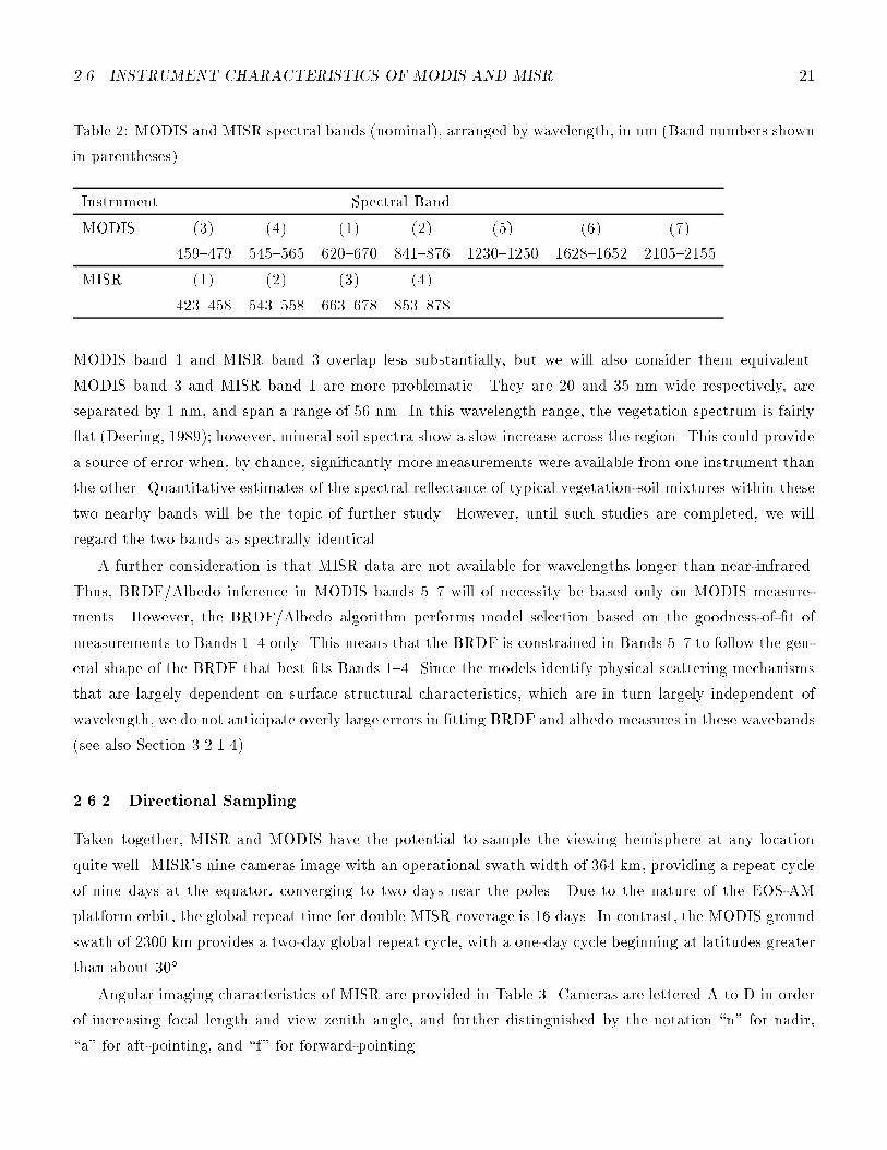
Table 2: MODIS and MISR spectral bands (nominal), arranged by wavelength, in nm (Band numbers shown
in parentheses).
Instrument Spectral Band
MODIS (3) (4) (1) (2) (5) (6) (7)
459{479 545{565 620{670 841{876 1230{1250 1628{1652 2105{2155
MISR (1) (2) (3) (4)
423{458 543{558 663{678 853{878
MODIS band 1 and MISR band 3 overlap less substantially, but we will also consider them equivalent.
MODIS band 3 and MISR band 1 are more problematic. They are 20 and 35 nm wide respectively, are
separated by 1 nm, and span a range of 56 nm. In this wavelength range, the vegetation spectrum is fairly
at (Deering, 1989); however, mineral soil spectra show a slow increase across the region. This could provide
a source of error when, by chance, signi�cantly more measurements were available from one instrument than
the other. Quantitative estimates of the spectral re ectance of typical vegetation-soil mixtures within these
two nearby bands will be the topic of further study. However, until such studies are completed, we will
regard the two bands as spectrally identical.
A further consideration is that MISR data are not available for wavelengths longer than near-infrared.
Thus, BRDF/Albedo inference in MODIS bands 5{7 will of necessity be based only on MODIS measure-
ments. However, the BRDF/Albedo algorithm performs model selection based on the goodness-of-�t of
measurements to Bands 1{4 only. This means that the BRDF is constrained in Bands 5{7 to follow the gen-
eral shape of the BRDF that best �ts Bands 1{4. Since the models identify physical scattering mechanisms
that are largely dependent on surface structural characteristics, which are in turn largely independent of
wavelength, we do not anticipate overly large errors in �tting BRDF and albedo measures in these wavebands
(see also Section 3.2.1.4).
2.6.2 Directional Sampling
Taken together, MISR and MODIS have the potential to sample the viewing hemisphere at any location
quite well. MISR's nine cameras image with an operational swath width of 364 km, providing a repeat cycle
of nine days at the equator, converging to two days near the poles. Due to the nature of the EOS-AM
platform orbit, the global repeat time for double MISR coverage is 16 days. In contrast, the MODIS ground
swath of 2300 km provides a two-day global repeat cycle, with a one-day cycle beginning at latitudes greater
than about 30�.
Angular imaging characteristics of MISR are provided in Table 3. Cameras are lettered A to D in order
of increasing focal length and view zenith angle, and further distinguished by the notation \n" for nadir,
\a" for aft-pointing, and \f" for forward-pointing.
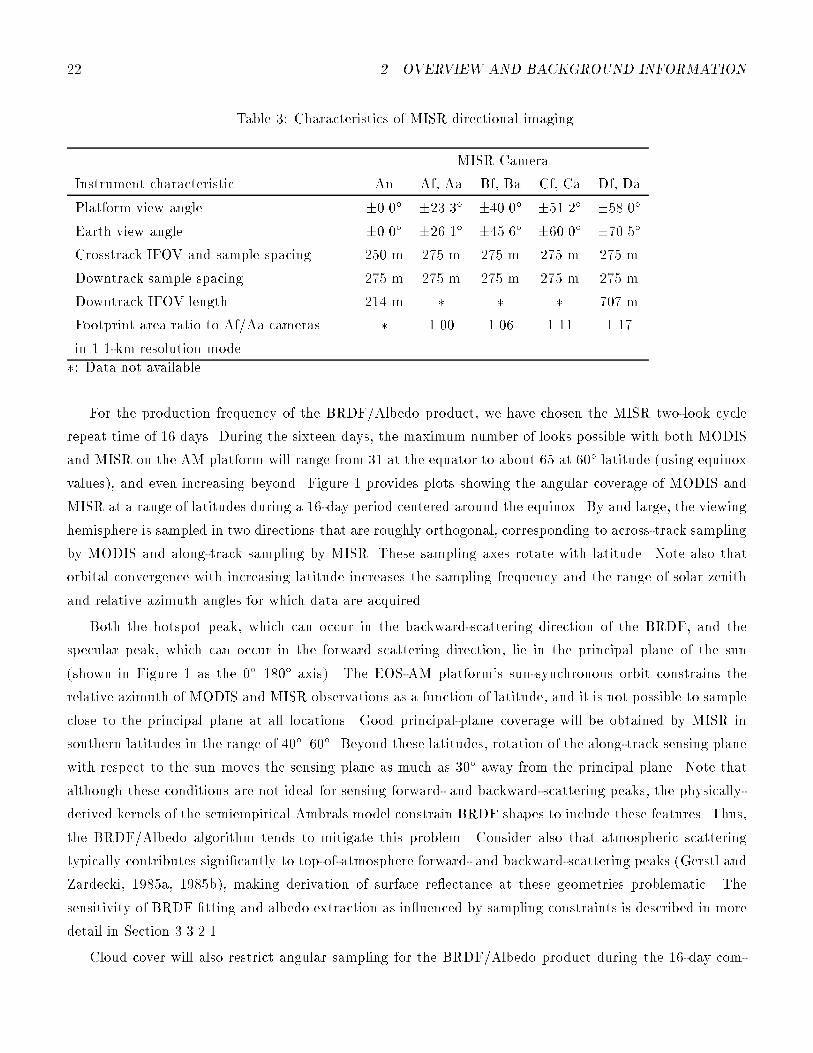
22 2 OVERVIEW AND BACKGROUND INFORMATION
Table 3: Characteristics of MISR directional imaging.
MISR Camera
Instrument characteristic An Af, Aa Bf, Ba Cf, Ca Df, Da
Platform view angle �0.0� �23.3� �40.0� �51.2� �58.0�Earth view angle �0.0� �26.1� �45.6� �60.0� �70.5�Crosstrack IFOV and sample spacing 250 m 275 m 275 m 275 m 275 m
Downtrack sample spacing 275 m 275 m 275 m 275 m 275 m
Downtrack IFOV length 214 m � � � 707 m
Footprint area ratio to Af/Aa cameras � 1.00 1.06 1.11 1.17
in 1.1-km resolution mode
�: Data not available
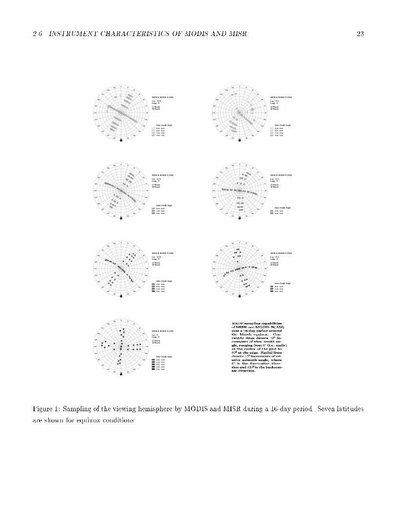
For the production frequency of the BRDF/Albedo product, we have chosen the MISR two-look cycle
repeat time of 16 days. During the sixteen days, the maximum number of looks possible with both MODIS
and MISR on the AM platform will range from 31 at the equator to about 65 at 60� latitude (using equinox
values), and even increasing beyond. Figure 1 provides plots showing the angular coverage of MODIS and
MISR at a range of latitudes during a 16-day period centered around the equinox. By and large, the viewing
hemisphere is sampled in two directions that are roughly orthogonal, corresponding to across-track sampling
by MODIS and along-track sampling by MISR. These sampling axes rotate with latitude. Note also that
orbital convergence with increasing latitude increases the sampling frequency and the range of solar zenith
and relative azimuth angles for which data are acquired.
Both the hotspot peak, which can occur in the backward-scattering direction of the BRDF, and the
specular peak, which can occur in the forward scattering direction, lie in the principal plane of the sun
(shown in Figure 1 as the 0�{180� axis). The EOS-AM platform's sun-synchronous orbit constrains the
relative azimuth of MODIS and MISR observations as a function of latitude, and it is not possible to sample
close to the principal plane at all locations. Good principal-plane coverage will be obtained by MISR in
southern latitudes in the range of 40�{60�. Beyond these latitudes, rotation of the along-track sensing plane
with respect to the sun moves the sensing plane as much as 30� away from the principal plane. Note that
although these conditions are not ideal for sensing forward- and backward-scattering peaks, the physically-
derived kernels of the semiempirical Ambrals model constrain BRDF shapes to include these features. Thus,
the BRDF/Albedo algorithm tends to mitigate this problem. Consider also that atmospheric scattering
typically contributes signi�cantly to top-of-atmosphere forward- and backward-scattering peaks (Gerstl and
Zardecki, 1985a, 1985b), making derivation of surface re ectance at these geometries problematic. The
sensitivity of BRDF �tting and albedo extraction as in uenced by sampling constraints is described in more
detail in Section 3.3.2.1.
Cloud cover will also restrict angular sampling for the BRDF/Albedo product during the 16-day com-
2.6 INSTRUMENT CHARACTERISTICS OF MODIS AND MISR 23
015
30
45
60
75
90
105
120
135
150
165180
195
210
225
240
255
270
285
300
315
330
345
70.00 - 74.99
75.00 - 79.99
80.00 - 84.99
85.00 - 89.99
Solar Zenith Angle
28 March 12 March
Long. - 0Lat. - 75 S
MISR & MODIS-N (AM)
015
30
45
60
75
90
105
120
135
150
165180
195
210
225
240
255
270
285
300
315
330
345
50.00 - 54.99
55.00 - 59.99
Solar Zenith Angle
28 March 12 March
Long. - 0Lat. - 55 S
MISR & MODIS-N (AM)
015
30
45
60
75
90
105
120
135
150
165180
195
210
225
240
255
270
285
300
315
330
345
30.00 - 34.99
35.00 - 39.99
40.00 - 44.99
Solar Zenith Angle
28 March 12 March
Long. - 0Lat. - 35 S
MISR & MODIS-N (AM)
015
30
45
60
75
90
105
120
135
150
165180
195
210
225
240
255
270
285
300
315
330
345
70.00 - 74.99
75.00 - 79.99
80.00 - 84.99
85.00 - 89.99
Solar Zenith Angle
28 March 12 March
Long. - 0Lat. - 75 N
MISR & MODIS-N (AM)
015
30
45
60
75
90
105
120
135
150
165180
195
210
225
240
255
270
285
300
315
330
345
50.00 - 54.99
55.00 - 59.99
60.00 - 64.99
Solar Zenith Angle
28 March 12 March
Long. - 0Lat. - 55 N
MISR & MODIS-N (AM)
015
30
45
60
75
90
105
120
135
150
165180
195
210
225
240
255
270
285
300
315
330
345
30.00 - 34.99
35.00 - 39.99
40.00 - 44.99
45.00 - 49.99
Solar Zenith Angle
28 March 12 March
Long. - 0Lat. - 35 N
MISR & MODIS-N (AM)
015
30
45
60
75
90
105
120
135
150
165180
195
210
225
240
255
270
285
300
315
330
345
10.00 - 14.99
15.00 - 19.99
20.00 - 24.99
25.00 - 29.99
30.00 - 34.99
Solar Zenith Angle
28 March 12 March
Long. - 0Lat. - 0
MISR & MODIS-N (AM)
Figure 1: Sampling of the viewing hemisphere by MODIS and MISR during a 16-day period. Seven latitudes
are shown for equinox conditions.
24 2 OVERVIEW AND BACKGROUND INFORMATION
positing period. Cloud cover is discussed further in Section 3.3.2.1 and Appendix B. The minimum number
of looks required for �tting a semiempirical model will depend on the exact distribution of view and azimuth
angles with respect to the principal plane, but can be taken roughly as 8. If a su�cient number of looks is
not available, information from supporting ancillary databases (previous BRDF/albedo product, land cover
type, and an ancillary global BRDF database that will be built as our knowledge grows) will be used to
limit or, if unavoidable, replace the inversion. Note that for some areas of the earth's land surface where
cloud cover is persistent, BRDF/Albedo retrieval may be infrequent.
2.6.3 Spatial Resolution
MODIS and MISR data have di�ering spatial resolutions. MISR provides a switchable resolution that
includes 275 m, 550 m, 1.1 km, and 2.2 km (250 m, 500 m, 1 km, 2 km for nadir camera), by combining
outputs of detectors in its linear arrays. However, since each of MISRs nine cameras image the ground
separately, their images must be registered after acquisition. Also, the individual bands acquired by each
camera require registration. Considering these factors, the MISR team plans to produce its global land
products at 1.1 km resolution in Space Oblique Mercator (SOM) projection. The resampling will also
include terrain relief correction for those areas with gentle slopes. Input to the BRDF/Albedo algorithm
will be Level 2 surface re ectance values produced at 1.1 km on the SOM grid.
The spatial resolution of the MODIS land bands varies by band. Red and infrared bands (1 and 2) are
sensed at 250-m resolution, while the remaining �ve bands (3{7) are acquired at 500 meters. These spatial
resolutions are nominal values at nadir. At o�-nadir angles, the ground projection of the detector's �eld
of view increases by a factor of about 2 in the along-track direction and 5 in the across-track direction to
the scan limit of �55�. From the viewpoint of BRDF retrieval, the far o�-nadir looks are most useful even
though they are imaged at a larger e�ective pixel size. A further complicating factor is that the instrument's
across-track 10-pixel scanning swath width increases with angle so that successive scans overlap (the \bow-
tie e�ect"). In fact, each ground location will be imaged twice at the far edge of the scan, appearing in two
successive scans.
The change in footprint with scan angle for MODIS will have the e�ect of smoothing the �tted BRDF
spatially, inducing an amount of spatial autocorrelation in the product. However, the MISR footprint, by
virtue of the separate focal length of each camera, the readout rate, and averaging method used for 1.1 km
resolution, increases only by 17 percent from nadir to D-camera imaging at 70� earth view zenith angle (see
Table 3). Thus, relatively few of the actual MODIS and MISR observations assembled in a 16-day period
will su�er from excessive pixel size.
Because the BRDF/Albedo is obtained from a set of measurements accumulated over a 16-day period,
Level 2 MODIS/MISR data must be gridded to Level 2G (based on the ISSCP sinusoidal grid) and binned
together before the Level 3 BRDF/Albedo product can be made.

25
3 ALGORITHM DESCRIPTION
3.1 THEORETICAL DESCRIPTION
Kernel-driven models for the bidirectional re ectance distribution function of vegetated land surfaces at-
tempt to describe the BRDF as a linear superposition of a set of kernels that describe basic BRDF shapes,
with the coe�cients or weights chosen to adapt the sum of the kernels to the given case. Typically, semiem-
pirical kernels are based either on one of several possible approximations to a radiative transfer scenario
of light scattering in a horizontally homogeneous plant canopy (e.g., a crop canopy), or on one of several
approximations feasible in a geometric-optical model of light scattering from a surface covered with vertical
projections that cast shadows (e.g., a forest canopy). Deriving a kernel of this nature requires simplifying
and manipulating a physical model for the BRDF until it reaches the form
R = c1k + c
2; (5)
in which k is a function only of view and illumination geometry, c1and c
2are constants containing physical
parameters, and R is the modeled value of the true BRDF, �.
The following discussion presents each of the kernels used in the BRDF/Albedo algorithm. The algorithm
that was developed for MODIS BRDF/Albedo Product is now known as \Ambrals" (Algorithm for MODIS
bidirectional re ectance anisotropies of the land surface), and the kernels applied jointly as the Ambrals
BRDF model. For more complete information on the theory and derivation of the kernels encompassed in
this algorithm, see Wanner et al. (1995, 1997).
3.1.1 Kernels
The Ross kernels are derived from a formula presented by Ross (1981) for the directional re ectance above
a horizontally homogeneous plant canopy calculated from radiative transfer theory in a single scattering
approximation. The Ross-thick kernel was derived and described by Roujean et al. (1992). It is based on
an approximation for large LAI values:
kthick =(�=2� �) cos � + sin �
cos �i + cos �v� �
4; (6)
c1
=4s
3�
�1� e
�LAI B�; (7)
c2
=s
3+ e
�LAI B
��s � s
3
�: (8)
In the kernel, �i and �v are zenith angles for illumination and view, respectively; � is the relative azimuth of
illumination and view directions; and � is the phase angle of scattering, cos � = cos �i cos �v+sin �i sin �v cos�.
In the constants, s is leaf re ectance (= leaf transmittance); �s is the (assumed isotropic) surface re ectance
of the soil or understory; LAI is the leaf area index; and B is the average of secants of possible view and
illumination zenith angles. For this formulation, a spherical leaf angle distribution is assumed. The Ross-thin
26 3 ALGORITHM DESCRIPTION
kernel simpli�es Ross's equation based on an approximation for small LAI values:
kthin =(�=2� �) cos � + sin �
cos �i cos �v� �
2; (9)
c1
=2sLAI
3�; (10)
c2
=sLAI
3+ �s: (11)
Although this kernel applies primarily to the case of a thin canopy of scatterers over a uniform background,
it can also be appropriate for a very dense, uniform canopy of high leaf area, since in that case the leaf layers
below the uppermost can act like a uniform background (Strahler et al., 1995).
The Li kernels are derived from the modeling approach of Li and Strahler (1986, 1992). In this approach,
the surface is taken as covered by randomly-placed projections (e.g., tree crowns) that are taken to be
spheroidal in shape and centered randomly within a layer above the surface. The BRDF is modeled as a
function of the relative areas of sunlit and shaded, crown and background that are visible from the viewing
position in the hemisphere. For the Li-sparse kernel, it is assumed that shaded crown and shaded background
are black, and that sunlit crown and background are equally bright. Under these circumstances, and with
some further approximations in the way that view and illumination shadows overlap, the Li-sparse kernel is:
ksparse = O(�i; �v; �)� sec �0i � sec �0v +1
2(1 + cos �0) sec �0v; (12)
where
O =1
�(t � sin t cos t) (sec �0i + sec �0v); (13)
cos t =h
b
qD2 + (tan �0i tan �
0v sin�)
2
sec �0i + sec �0v; (14)
D =qtan2 �0i + tan2 �0v � 2 tan �0i tan �
0v cos�; (15)
cos �0 = cos �0i cos �0v + sin �0i sin �
0v cos�; (16)
�0 = tan�1
�b
rtan �
�; (17)
In these expressions, b is the vertical radius of the spheroid; h is the horizontal radius of the spheroid; and
is the height of the center of the spheroid. For this model, and
c1
= C ��r2
; (18)
c2
= C: (19)
Here, C is the brightness of sunlit surface, and � is the count density of spheroids (number of spheroids
per unit area). The sun zenith angle dependence of C may be approximated as C= cos�i (Schaaf, Li and
Strahler, 1994).
3.1 THEORETICAL DESCRIPTION 27
The Li-dense kernel di�ers from the Li-sparse kernel in that it accommodates mutual shadowing. It
assumes a random distribution of crown heights to maximize the geometric-optical e�ect in a dense ensemble
of canopies.
kdense =(1 + cos �0) sec �0v
sec �0v + sec �0i � O(�0i; �0v)� 2; (20)
c1
=C
2(1� �); (21)
c2
= C + (G� C)�: (22)
These kernels are not yet linear in that they still contain two parameters, namely the ratios and ,
describing crown shape and relative height. For the present, we �x each parameter using a spherical shape
close to the ground for the Li-sparse kernel (b=r = 1, h=b = 2) and a higher prolate shape for the Li-dense
kernel (b=r = 2:5, h=b = 2). The �xed parameters for the Li-sparse kernel are intended for sparser vegetation
covers exhibiting geometric-optical shadowing e�ects, such as shrublands or woodlands. It also �ts some
rough surfaces, such as plowed �elds. The Li-dense kernel is intended to capture the three-dimensional
mutual shadowing e�ects that occur in conifer forests and other vegetation covers with tall plant crowns.
As do most available BRDF models, all of these kernels assume that the BRDF depends only on the
relative azimuth between the solar and the viewing direction. This symmetry may not be realized in
some natural situations, for example for row e�ects or other preferential orientation of plants for ecological
reasons. However, at this point we think that introducing another degree of freedom into the modeling is not
warranted in view of the additional retrieval uncertainties this would introduce and our lack of knowledge
concerning the relative importance of such e�ects. In a post-launch periods extensions of the modeling to
non-symmetric BRDFs are possible.
In anticipation of situations in which forward scattering by water surfaces, as for example in rice paddies
or ood zones, produce some specular re ection form water surface facets, we have provisionally added
a kernel based on the Cox-Munk model (1954) for sea-surface scattering. With some assumptions, the
Cox-Munk model can be made to �t the form R = c1k + c2 , in which the kernel kspec, is
kspec =1
cos �i
1� tan2 �n
�2
!� 1 if
tan2 �n�2
� 1;
kspec = �1 else: (23)
In this expression, �2 is the slope variance, given as �2 = 0:003 + 0:00512w, with w as the wind speed, in
m/sec. The parameter �n is de�ned by
cos2 �n =1
2
(cos �i + cos �v)2
1 + cos�
!: (24)
The constants c1and c
2for this model are
c1= c
2=
�(0; �)
4��2; (25)
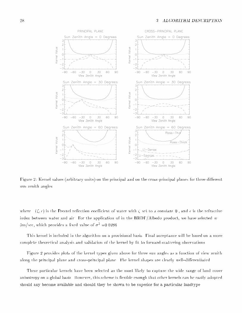
28 3 ALGORITHM DESCRIPTION
Figure 2: Kernel values (arbitrary units) on the principal and on the cross-principal planes for three di�erent
sun zenith angles.
where �(�; �) is the Fresnel re ection coe�cient of water with � set to a constant 0., and � is the refractive
index between water and air. For the application of in the BRDF/Albedo product, we have selected w =
5m/sec, which provides a �xed value of �2 =0.0286.
This kernel is included in the algorithm on a provisional basis. Final acceptance will be based on a more
complete theoretical analysis and validation of the kernel by �t to forward-scattering observations.
Figure 2 provides plots of the kernel types given above for three sun angles as a function of view zenith
along the principal plane and cross{principal plane. The kernel shapes are clearly well{di�erentiated.
These particular kernels have been selected as the most likely to capture the wide range of land cover
anisotropy on a global basis. However, this scheme is exible enough that other kernels can be easily adopted
should any become available and should they be shown to be superior for a particular landtype.
3.1 THEORETICAL DESCRIPTION 29
3.1.2 Kernel-Driven Models
A complete kernel-driven semiempirical model is formulated as a linear combination of kernels. Most suitably
it has the form
R = fiso + fgeokgeo + fvolkvol; (26)
which is derived from adding appropriate choices of geometric-optical surface-scattering and radiative-
transfer volume-scattering kernels, each multiplied by a proportion � or (1��) that weights the contributionof each model. These proportions may be regarded as the areal proportions of land cover types exhibiting
each type of scattering (neglecting multiple scattering between the two components), or as mixing propor-
tions for land cover types that display both a volume{scattering and a geometric{optical contribution to the
BRDF. The quantities and are the respective kernels; the factors fgeo and fvol are their respective weights;
and the term fiso is the isotropic contribution. The formulae for fiso, fgeo, and fvol are shown in Table 4.
In the inversion and �tting of a semiempirical model to data, estimates of the weights f are retrieved from
bidirectional re ectances and speci�cation of viewing and illumination positions. Although this objective
satis�es many of the goals of the BRDF/Albedo product, the existence of formulae for the weights f in terms
of physical parameters could provide for direct inference of physical parameters from the weight values �tted
(see Section 2.4). This possibility will be explored in the postlaunch phase as a research topic.
The kernel-driven semiempirical BRDF model using either the Ross-thin or the Ross-thick model for vol-
ume scattering and either the Li-sparse or the Li-dense kernel (using the crown height and shape parameters
given above) are known and will be referred to as the Ambrals BRDF model (Wanner et al., 1997).
3.1.3 The Modi�ed Walthall Model
Empirical models can be understood as being of the kernel-driven model type as well, where the kernels
are empirical functions. An example is the modi�ed Walthall model, derived by Walthall et al. (1985) and
improved by Nilson and Kuusk (1989). It has the form
R = p0
��2
i + �2
v
�+ p
1�2
i �2
v + p2�i�v cos�+ p
3: (27)
Note that this is the same form as the semiempirical models discussed above | it is comprised of a weighted
superposition of functions of angles, and the weights p are the parameters of the model. As a consequence,
models like the modi�ed Walthall model can be processed along with linear semiempirical models by the
same linear inversion scheme.
3.1.4 Advantages of Linear Models
Linear models have a number of advantages in the context of global data processing. Linearity in BRDF
models is comprehensively discussed by Lewis (1995) and demonstrated with the modi�ed Walthall model. A
�rst and foremost advantage is that any linear model can be inverted analytically through matrix inversion for
the system of equations obtained by setting the derivative of the error function to zero (see Section 3.2.1).

30 3 ALGORITHM DESCRIPTION
Table 4: Semiempirical weight formulas
Model Weight Formulae
Ross-thin plus Li-sparse: fiso = �C + (1� �)�sLAI3
+ �s
�,
fgeo = �C ��r2,
fvol = (1� �) 2sLAI3�
.
Ross-thick plus Li-sparse: fiso = �C + (1� �)�s3+ e�LAI B
��0� s
3
��,
fgeo = �C ��r2,
fvol = (1� �) 4s3�
�1� e�LAI B
�.
Ross-thin plus Li-dense: fiso = �C + (1� �)�sLAI3
+ �s
�,
fgeo = �C2,
fvol = (1� �) 2sLAI3�
.
Ross-thick plus Li-dense: fiso = �C + (1� �)�s3+ e�LAI B
��0� s
3
��,
fgeo = �C2,
fvol = (1� �) 4s3�
�1� e�LAI B
�.
This provides direct estimates of the parameters fiso, fgeo, fvol and while avoiding numerical inversion
problems.
Second, both the directional-hemispherical and bihemispherical integrals of the BRDF (black-sky and
white-sky albedos) may be precalculated for each kernel individually. The albedo of a model then is simply
the sum of the kernel albedos, weighted by f values. By using a look-up table, numerical integration of the
models can thus be avoided.
Third, linear BRDF models scale linearly in space if adjacency e�ects are assumed to be small. This
allows for mixed pixel cases, as indicated by the areal proportion parameter in the model factors listed above.
This feature also allows for the scaling of BRDF and albedo from one spatial resolution up to a coarser one,
e.g., to a particular resolution needed for a climate model. Finally, since some of the parameters driving the
models are dependent on wavelength while others are not (e.g., structural parameters), it may be possible
to extract all or some of them from multiband analysis, making assumptions about the others.
3.1.5 Validation of Semiempirical Models
3.1.5.1 Fit of Semiempirical Models to Ground Data
Note: A full detailed report on the validation of the kernel-driven Ambrals semiempirical BRDF model
is given in Appendix A. Please refer to this appendix for data sources, tables, �gures and an in-depth
discussion.
The ability of the Ambrals semiempirical BRDF model to describe naturally occurring BRDF shapes
was tested using 27 di�erent data sets measured on the ground or from airborne instruments. These data

3.1 THEORETICAL DESCRIPTION 31
sets include a wide variety of land cover types as will be encountered in global remote sensing. Among
these are barren types (soils of di�erent roughnesses), sparsely vegetated types (both patchy and uniformly
sparse), dense vegetation (both broadleaf crops, and grasses and cereal crops), and forests (both needleleaf
and broadleaf). When using such data sets to validate a BRDF model to be used in remote sensing at a
spatial resolution of one kilometer, a scaling problem clearly exists. However, currently no good data sets
over a variety of di�erent land cover types exists that has both coarse spatial resolution and good angular
sampling at several di�erent solar zenith angles. Therefore, �eld-measured data sets are still indispensable
for model validation. If the di�erent BRDF shapes met in the �eld are �tted well by a BRDF model,
it may be reasonably expected that the BRDFs observed for similar vegetation types at a scale of 1 km,
which will probably be smoother, will also be �t well. In case of mixed land covers, the Ambrals BRDF
model is expected to be better suited for modeling the mix than most other BRDF models (which were
derived assuming homogeneous scenes) due to its linear superpositioning approach. Scaling issues are further
discussed in Appendix F.
The 27 observed BRDF data sets were inverted for all available bands (mostly red and near-infrared)
and all solar and view angles simultaneously. None of these data sets were �tted with an RMS absolute
error of more than 0.046, the average RMSE being 0.034. Furthermore, the correlation coe�cient between
the modeled and the observed re ectances was determined for the red band and the near-infrared band. In
the red band, 12 of the 27 data sets showed a correlation coe�cient larger than 0.9; 18 of 27 one larger than
0.8; and 23 of 27 one larger than 0.75. Only one data set had a correlation coe�cient smaller than 0.7, but
this data set was found to have irregular features in the observed red band re ectances. In the near-infrared
band, 13 of 27 data sets showed correlation coe�cients larger than 0.9, 23 of 27 had ones larger than 0.8,
and 26 of 27 had ones larger than 0.75. These values indicate a reasonable agreement between modeled and
observed re ectances, validating the Ambrals BRDF model.
With respect to the kernel combinations found to best represent each land cover type, two results are
mainly of interest. First, there is some correlation between the type of land cover being modeled and the
kernel combinations producing the best �t. In shadow-casting cases like a plowed �eld or a sparse forest, the
Li-sparse kernel was dominant. In cases of a dense forest, the Li-dense kernel produced the lowest RMSE.
In the case of dense crops, kernel combinations including the Ross-thick kernel produced best �ts. The
second �nding is that even though di�erent kernel combinations may produce small values of the RMSE
for a particular case, visual inspection of �ts reveals that the model with the lowest RMSE indeed �ts the
observed data better than a model with a slightly higher RMSE, demonstrating the bene�t of allowing
multiple kernel combinations.
Validation of the Ambrals BRDF model was carried out in parallel to an evaluation of the modi�ed RPV
model (Rahman et al., 1993b; Engelsen et al., 1996). The comparison shows that the Ambrals model results
are very similar, perhaps even slightly better, than those for the modi�ed RPV model.
Please refer to Appendix A for a full report of these validation results, including tables, �gures and more
detailed analysis.
32 3 ALGORITHM DESCRIPTION
3.1.5.2 Inversion and Fitting of Semiempirical Models to ASAS Data Researchers at University
College London recently applied two semiempirical models to directional image data obtained for a semiarid
region of West Africa near Niamay, Niger (Barnsley et al., 1996; Lewis et al., 1995; see Appendix J). In
this study, NASA's Advanced Solid-state Array Spectrometer (ASAS) (Irons et al., 1991) acquired image
data from an aircraft platform over the HAPEX-Sahel west central, east central and southern super-sites
on various dates during September 3{17, 1992. The ASAS acquires images at ten sensor view angles during
a single overpass | one at nadir and nine others at 15� increments between 75� forward and 60� aft of
the aircraft platform on which it is mounted. These images are recorded in 64 continuous narrow spectral
wavebands in wavelengths ranging from the visible to the near-infrared. Spatial resolution is about 4 m.
Data processing involved manipulating the multiple{view{angle and multiple ight{line ASAS image data
in four steps: (i) geometric registration; (ii) radiometric correction; (iii) atmospheric correction; and (iv)
estimation of the surface (spectral) BRDF and albedo through BRDF model inversion.
Geometric registration of the multiple-view-angle and multiple ight-line data was perhaps the most
problematic task. Standard polynomial warping techniques are generally unable to cope with the very high
frequency, localized geometric distortions present in most airborne scanner images. Consequently, Barnsley
et al. (1996) used an automated image registration procedure based on \interest point" extraction and
area-based matching of small patches of image around each interest point (Allison et al. 1991, Allison
and Muller 1992) to de�ne an initial polynomial mapping followed by pixel patch-by-pixel patch (typically
15 x 15 pixels) matching using adaptive least-squares image correlation (Otto and Chau, 1989). These
techniques are capable of registering multiple view-angle ASAS images to subpixel accuracy (<0.4 pixels)
globally throughout the scene (Allison et al. 1994). In this case, each of the o�-nadir images was registered
to the nadir view. Radiometric correction was e�ected using gain values provided by NASA to convert
the instrument's raw DN values to spectral radiances. Atmospheric correction was applied by use of the 6S
atmospheric correction code (Vermote et al. 1994) with atmospheric parameters derived from sun photometer
data (Brown de Colstoun et al., 1996).
With registered and corrected data at hand, the Walthall and Roujean models were inverted and �tted
to the data on a pixel-by-pixel basis (Barnsley et al., 1996; see Appendix J). This allowed the construction
of images of the weights associated with each term of each model. The nadir re ectance images in the blue
and near-infrared bands have low contrast and appear noisy. In these bands, the models seem to be �tting
noise rather than signal. In contrast, the green and red bands show a coherent scene structure. The �rst
parameters from both Walthall and Roujean models are strongly related to overall brightness and thus mimic
the nadir re ectance. The second and third parameters of the Walthall model show little spatial structure,
although some bright and dark spots seem to correlate well with particular patches in the nadir image.
In contrast, the Roujean model shows strong spatial structure in both the �rst and second parameters.
The second parameter is the weight of the geometric kernel, which seems to vary inversely with the �rst
parameter. This indicates that the BRDF becomes more isotropic with increasing brightness, which is not
unexpected if multiple scattering increases with brightness. The �ne texture in the images of the third
3.1 THEORETICAL DESCRIPTION 33
parameter may be related to �ne errors in registration, rather than real changes in BRDF within the scene.
Overall, the weight of the third parameter is quite low, indicating that volume scattering is not important
for these surfaces. Since vegetation is quite sparse over most of the target area, this is not unreasonable.
These results demonstrate that a pixel-by-pixel inversion of empirical/semiempirical models is possible, and
that the model parameters vary systematically in a meaningful spatial pattern.
More recently, (Muller and Disney, 1997; Muller et al., 1997a, b) have processed all of the ASAS data
into surface directional re ectance for all three study sites. Preliminary results are presented in Appendix F
of two applications of these spectral directional re ectance �elds. In the �rst application, a study was
performed (results shown here for Southern Super Site and West Central Super Site) of the impact of spatial
resolution on the type of models which are retrieved. The results indicate that at 3m resolution, the modi�ed
Walthall model is chosen consistently over two di�erent cover types (millet and savannah) whereas at 30m,
90m and 240m the RossThick{LiDense is primarily chosen for the same regions. This indicates that we
may have di�culties using �eld spectro-radiometric data acquired at around a couple of meters to validate
MODIS/MISR derived BRDF/albedo over sparse canopies.
In the second application (Muller et al., 1997a), the ASAS modi�ed Walthall results were used to generate
training statistics for a TM supervised maximum likelihood classi�cation after registration and resampling
of the ASAS directional re ectance values. This has allowed a spectral albedo map to be produced for
the whole of the Southern Supersite area at 30m for use in simulation and testing of the MODIS/BRDF
inversion algorithm. In addition, broadband albedo data are available for validating these ASA/TM-derived
spectral albedos to assess how accurate the inverted albedos will be (see Appendix G).
In the �nal application, a Monte Carlo ray-tracing system (Lewis and Muller, 1992) was used together
with geometrical-optical models of millet plants to simulate the radiance at the ASAS sensor, and these
values were compared with those extracted from ASAS after atmospheric correction (Muller et al., 1997b).
The MCRT allows studies to be made of the signi�cance of the biophysical parameters included within
the semiempirical models as well as the impact of di�erent sampling scenarios (MODIS only, MISR only,
MODIS+MISR, cloud-cover impacts) on the accuracy of the derived BRDF parameters and spectral as well
as broadband albedo values (see Appendix H for more details).
3.1.5.3 Inversion and Fitting of Semiempirical Models to AVHRR Data As part of an Euro-
pean Union consortium investigating land cover change in the Sahel, researchers at UCL have also been
investigating the application of the Ambrals model to AVHRR data (see Appendix J). Six months (May{
October 1992) of LAC derived surface re ectance data of the HAPEX-Sahel grid square have been processed
using the model and aspects of model �t and model selection investigated (Lewis and Ruiz de Lope, 1996).
The results indicate that the Ambrals kernels are able to describe the shape of the BRDF (processed
on a 16-day window, 1-day step, moving window) well over the period of study. Relatively large errors
in model �t can, however, occur during the rainy season, due to variations in the surface re ectance on
a sub-16-day timescale. In spite of this, the trends in normalized re ectance, albedo and BRDF model
34 3 ALGORITHM DESCRIPTION
parameters are generally well-maintained. The temporal trajectory of these model parameters is currently
being investigated with a view to providing information on variations in the surface cover.
The main kernel selection criterion in Ambrals, the RMSE in model �t, is found in many cases not
to provide very consistent results (either temporally and spatially). It is understood that Ambrals will
have to make use of additional information in aiding kernel selection, and so the team at UCL have been
investigating the issues involved. Currently, an approach that considers temporal consistency in the main
selection criterion, weighted by the RMSE is being tested. Early results indicate that this is indeed promising,
and that it can be implemented e�ciently within Ambrals.
In addition to this research, work is currently underway testing the application of Ambrals to the AVHRR
Path�nder (PAL) dataset for Africa north of the Equator. Two years of data have been processed so far
(1989 and 1992) and the 1992 results compared with the LAC data over HAPEX-Sahel described above.
While many of the trends observed appear to be similar in the two datasets, the magnitude of the trends
are very di�erent, probably mainly due to the poor atmospheric correction of the data (PAL corrects for
only Rayleigh scattering and ozone absorption).
3.2 THE MODIS BRDF/ALBEDO ALGORITHM
3.2.1 Model Inversion and Retrieval of BRDF and Albedo
3.2.1.1 Theoretical Background: Inversion A kernel-driven model has the form
R(�i; �v; �;�; I1; I2) =nX
k=1
fk(I1(�)) kk(�i; �v; �;�; I2(�)); (28)
or, for a set of discrete values of the BRDF,
Rl(�) =nX
k=1
fk(I1(�))kkl(I2(�)); (29)
where R is the re ectance; �i and �v are the zeniths of view and illumination, respectively; and � is the
relative azimuth; � is the waveband; I1and I
2are lists of parameters describing light scattering in the
scene, with the kernel-internal parameters; the parameters of the BRDF model; and kk the kernels, where
the index stands for a particular viewing and illumination geometry, (�i; �v; �)l. This formula expresses that
kernel-driven BRDF models for a waveband are formulated as a superposition of basic BRDF shapes, where
the kernel shapes k are functions of viewing and illumination geometry only (provided that the parameters
I2have been �xed); and the respective contribution of each kernel value kkl to the resulting re ectance is
given by the corresponding parameter or weight fk , depending on the internal parameters as a function of
wavelength. The number of kernels to be superimposed is n. Usually three kernels are chosen | the �rst
is the constant unity, representing isotropic scattering, the second represents volume scattering, the third
surface scattering.
An observation consists of N directional measurements �0l(�) where l runs from 1 to N . The di�erence
between the modeled and the observed re ectances is measured by an error function E, which generally is
3.2 THE MODIS BRDF/ALBEDO ALGORITHM 35
de�ned in the following way:
E2(�) =
1
d
NXl=1
(�0l(�)�Rl(�))2
wl(�); (30)
where wl are the weights attributed to the respective observations. Choices for error weights include wl(�) =
1, wl(�) = �0l(�), wl(�) = Rl(�), or wl(�) = �02l (�). The quantity d is the degrees of freedom, i.e., d = N�n.E is taken as the root-mean-square error, or RMSE.
Inversion of the BRDF model aims at determining the parameters k of the model. The parameters
wanted are those for which E attains a minimum. In other words, those k for which (dropping explicit
mention of waveband dependencies)
@E2
@fj=
1
d
NXl=1
2
wl(�0l � Rl)
@�0l
@fj� @Rl
@fj
!= 0; (31)
provided that the solution to this equation is a minimum and not a maximum or a saddle point. The
derivative of the observed re ectances with respect to the parameters is zero, of course, but for modeled
re ectances @Rl=@fj we have
@Rl
@fj=
@
@fj
nX
k=1
fkkkl
!=
nXk=1
@fk
@fjkkl + fk
@kkl
@fj
!=
nXk=1
�kjkkl = kjl; (32)
where �kj = 1 if k = j, otherwise 0.
Thus,
@E2
@fj=
1
d
NXl=1
2
wl
(�0l � Rl)kjl = 0; (33)
orNXl=1
�0lkjl
wl=
NXl=1
Rlkjl
wl=
NXl=1
NXk=1
fkkklkjl
wl: (34)
Introducing the vector V and the Matrix M as
Vj =NXl=1
�0lfjl
wl; (35)
Mjk =NXl=1
kjlkkl
wl
; (36)
we can write the equation for the parameters delivering the best �t as
Vj =nX
k=1
Mjkfk (37)
and arrive at the solution
fk =nX
j=1
M�1jk Vj (38)
36 3 ALGORITHM DESCRIPTION
for the parameters. Thus, the BRDF model has been analytically inverted via an analytical solution to the
single stationary point of the error function. From physical arguments, we can show that this is the global
minimum (Lewis, 1995).
However, the values fk that are obtained by this procedure are not constrained to lie within proper
physical bounds. For example, if the kernels in a particular semiempirical model are inappropriate for the
surface type, the best �t might require a negative weight on one of the kernels, which is not physically
possible given the physical derivation of the weight functions. Although not yet implemented, it is a simple
matter to constrain the solution such that the fk lie within reasonable bounds via Lagrange multipliers
(Lewis, 1995). In the event that the model with the constrained solution actually presents the lowest error
among all semiempirical models, a ag will carry forward the information that the �t was constrained and
thus is of lower con�dence.
3.2.1.2 Advantages of the Kernel-Based Approach The algorithm that was developed for MODIS
BRDF inversion and albedo computing, (known as \Ambrals", the Algorithm for MODIS bidirectional
re ectance anisotropies of the land surface) was programmed in a kernel-oriented, rather than model-oriented,
fashion so that it would be both exible and e�cient. Values of all kernels occurring at the viewing and
illumination angles at hand are computed and tabulated so that the functions have to be processed only
once for each geometric situation and each kernel . After that, each kernel value kkl is referred to via a
look-up table. This allows rapid computing, for example, of the matrixM as a function of the model chosen,
or of the re ectances resulting from the parameters found (needed, for example, for calculating the RMSE).
Since the suite of models to be inverted share kernels, this makes the code e�cient by avoiding duplication
of computations. Trigonometric expressions that are shared by several kernels are also computed only once.
The algorithm's kernel-based approach has the additional advantage of easily allowing an increase in the
number of kernels and of formulating new models by allowing the free combination of any number of kernels.
This feature is also essential in the spatial degrading of the BRDF/albedo product (see Section 3.3.2 and
Appendix F).
3.2.1.3 Matrix Inversion and Error Function Used Inversion of the matrix Mjk =P
l kjlkkl=wl
is performed by a standard LU decomposition algorithm. In the general case, is dependent on wavelength
and the inverse needs to be calculated for each band separately. However, if the weights wi are chosen to
be independent of the wavelength, M is independent as well, assuming that if the kernels contain internal
physical variables I2these have been set to �xed values. Then for each set of observations sampling a given
BRDF, M needs to be inverted only once for all bands observed.
This is the case with the error function chosen for the current BRDF inversion problem, which was
selected to measure the mean squared absolute deviation of modeled and observed re ectances,
E2(�) =
1
d
NXl=1
(�0l � Rl)2 (39)
3.2 THE MODIS BRDF/ALBEDO ALGORITHM 37
i.e., wl was chosen to be 1. The RMSE of a given model is de�ned as the root of the average of E2 over all
bands, although for selection of the best-�tting model, only bands 1{4 are considered. The weighting function
wl was chosen in this way because it allows most accurate modeling of the commonly found upturning of
the BRDF for large zenith angles, which is of importance in deriving albedo; the cost is a reduced relative
accuracy of re ectances with a low value. Studies on penalty functions and more complex forms of will be
conducted in the near future.
3.2.1.4 Model Selection In the MODIS processing scenario, level-2 re ectances that have been cloud
cleared and atmospherically corrected are binned into the MODIS level-2G grid over a period of 16 days
and combined with all MISR observations acquired during that same time. The data from each image are
interpolated to a spatial resolution of one kilometer, where each observation is weighted by the respective
overlap between the grid cell and the observation footprint. Quality information associated with the data
is translated to quality coe�cients that are used to weight individual observations in the subsequent BRDF
inversion. This allows special consideration of data where, for example, atmospheric correction was di�cult
or aerosol information was taken from standard tables because no aerosol retrievals were available.
The directional observations thus assembled are then analyzed by inverting the �ve model variants as
decribed above to �nd the Ambrals kernel combination that �ts the observations best. The four bands
common to MODIS and MISR are inverted �rst. The model chosen as best from this analysis is then
applied to the three remaining bands, in which only MODIS data are available. The model parameters
found are written to output along with extensive quality control data and other information necessary for
an assessment of the product. Integration of the BRDF is carried out to provide black-sky and white-sky
albedos.
In general, the kernel combination which provides the �t with the smallest root band-averaged mean
squared error (RMSE) as described above is selected. The two cases where an exception is made are if the
RMSE found is large, or angular sampling coverage is bad enough to mistrust the inversion, either because
observations span only a small angle range or their number is too small. In these cases information from
the supporting ancillary databases is used to limit the inversion.
If angular sampling is good but the RMSE found is high, the kernel combination suggested by the ancillary
data (previous BRDF, the historical accumulated BRDF database, land cover type, and topography) is used
instead (if the resulting RMSE is not much worse). The model parameters are still derived from a full
inversion of the re ectances.
If angular sampling is bad or the number of re ectances available is too small, a full inversion cannot
be trusted and gaps in the product would result. In this case, the BRDF kernel combination and model
parameters suggested by the ancillary databases will be used, but the magnitude of the BRDF (the isotropic
constant of the model) will be adjusted to the observed re ectances. Through this the shape but not the
magnitude of the BRDF will be �xed. This procedure also guarantees that the re ectance information
available in cases not permitting a full BRDF inversion will not be simply lost but used to the extent

38 3 ALGORITHM DESCRIPTION
possible.
In each case, the source of the resulting BRDF information will be recorded so that users can �lter the
output according to their needs. The ancillary database accumulating BRDF knowledge over time, keyed
by season, and the relationships between land cover type and BRDF used will be established post-launch
from the data observed and updated at intervals.
The exibility of the Ambrals model means that the mathematical expressions used on adjacent pixels
may be slightly di�erent. While this is expected to provide the best BRDF and albedo information on a per-
pixel basis, it may introduce too much complexity in applications where a much simpler uniform approach
is desired. As a consequence, the MODIS BRDF/albedo product will always also provide the full inversion
results for the modi�ed Walthall BRDF model [Walthall et al., 1985; Nilson and Kuusk, 1989]. This model
is purely empirical and is expected to produce results of reduced accuracy, particularly under conditions of
sparse angular sampling. But the simplicity of the mathematical expression used and the fact that it will
be the same for all pixels make it attractive for applications where such a reduced accuracy is acceptable.
3.2.1.5 Albedo Calculation Deriving the directional-hemispherical and bihemispherical integrals from
the BRDF requires, in the general case, a numerical integration of the BRDF, which is computationally very
costly if it is to be performed routinely for a global product at the 1-kilometer scale. The linearity of
kernel-driven models with respect to their parameters allows a handy way out of this dilemma. Since the
integration is with respect to the occurring angles and only the kernels depend on these angles, and since
these are known in advance, the integral of the BRDF may be written as a weighted sum of the integrals
of the kernels, where the weights are the same as those in the BRDF model. The integrals of the kernels
may, then, be computed numerically in advance (once) and the results stored in a table. Albedo calculations
are then reduced to forming a simple linear combination of these tabulated values. This applies to both
black-sky and white-sky albedo. The black-sky albedo of the individual kernels is tabulated as a function of
solar zenith, where the zenith is incremented by a small amount (e.g., 0:25� | although the table is not large
in any case) and interpolated for intermediate values. Therefore, black-sky albedo at any solar zenith angle
and white-sky albedo for both models (the \best �t" model and the Walthall model) can be constructed
with almost no computational e�ort directly from the model parameters using these small look-up tables of
precomputed kernel integrals which will be provided to users with the product. Broadband albedos will be
given in a similarly parameterized form.
In addition, the product will provide a single set of black-sky albedo values for the median sun angle for
the suite of observations that were inverted to �t the BRDF. (Note that the black- and white-sky albedos
are provided in each of seven spectral bands, two aggregated bands and one broad band.)
3.2.1.6 Algorithm Flow and Execution Figure 3 demonstrates data ow in connection with the
BRDF/Albedo algorithm. Surface re ectances produced by the MODIS and MISR atmospheric correction
algorithms are passed into a BRDF subsetting and database compilation process along with selected infor-
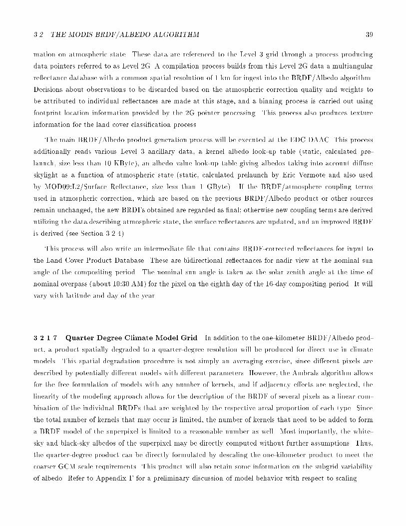
3.2 THE MODIS BRDF/ALBEDO ALGORITHM 39
mation on atmospheric state. These data are referenced to the Level 3 grid through a process producing
data pointers referred to as Level 2G. A compilation process builds from this Level 2G data a multiangular
re ectance database with a common spatial resolution of 1 km for ingest into the BRDF/Albedo algorithm.
Decisions about observations to be discarded based on the atmospheric correction quality and weights to
be attributed to individual re ectances are made at this stage, and a binning process is carried out using
footprint location information provided by the 2G pointer processing. This process also produces texture
information for the land cover classi�cation process.
The main BRDF/Albedo product generation process will be executed at the EDC DAAC. This process
additionally reads various Level 3 ancillary data, a kernel albedo look-up table (static, calculated pre-
launch, size less than 10 KByte), an albedo value look-up table giving albedos taking into account di�use
skylight as a function of atmospheric state (static, calculated prelaunch by Eric Vermote and also used
by MOD09:L2/Surface Re ectance, size less than 1 GByte). If the BRDF/atmosphere coupling terms
used in atmospheric correction, which are based on the previous BRDF/Albedo product or other sources
remain unchanged, the new BRDFs obtained are regarded as �nal; otherwise new coupling terms are derived
utilizing the data describing atmospheric state, the surface re ectances are updated, and an improved BRDF
is derived (see Section 3.2.4).
This process will also write an intermediate �le that contains BRDF-corrected re ectances for input to
the Land Cover Product Database. These are bidirectional re ectances for nadir view at the nominal sun
angle of the compositing period. The nominal sun angle is taken as the solar zenith angle at the time of
nominal overpass (about 10:30 AM) for the pixel on the eighth day of the 16-day compositing period. It will
vary with latitude and day of the year.
3.2.1.7 Quarter Degree Climate Model Grid In addition to the one-kilometer BRDF/Albedo prod-
uct, a product spatially degraded to a quarter-degree resolution will be produced for direct use in climate
models. This spatial degradation procedure is not simply an averaging exercise, since di�erent pixels are
described by potentially di�erent models with di�erent parameters. However, the Ambrals algorithm allows
for the free formulation of models with any number of kernels, and if adjacency e�ects are neglected, the
linearity of the modeling approach allows for the description of the BRDF of several pixels as a linear com-
bination of the individual BRDFs that are weighted by the respective areal proportion of each type. Since
the total number of kernels that may occur is limited, the number of kernels that need to be added to form
a BRDF model of the superpixel is limited to a reasonable number as well. Most importantly, the white-
sky and black-sky albedos of the superpixel may be directly computed without further assumptions. Thus,
the quarter-degree product can be directly formulated by descaling the one-kilometer product to meet the
coarser GCM scale requirements. This product will also retain some information on the subgrid variability
of albedo. Refer to Appendix F for a preliminary discussion of model behavior with respect to scaling.
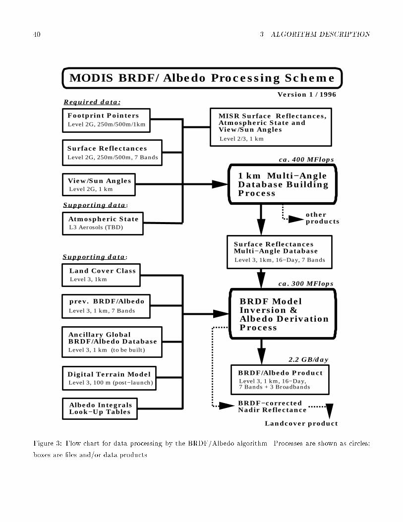
40 3 ALGORITHM DESCRIPTION
MODIS BRDF/Albedo Processing Scheme
BRDF−corrected Nadir Reflectance
ca. 400 MFlops
ca. 300 MFlops
1 km Multi−Angle Database BuildingProcess
Footprint PointersLevel 2G, 250m/500m/1km
Surface ReflectancesLevel 2G, 250m/500m, 7 Bands
View/Sun AnglesLevel 2G, 1 km
MISR Surface Reflectances, Atmospheric State and View/Sun AnglesLevel 2/3, 1 km
BRDF ModelInversion & Albedo Derivation Process
BRDF/Albedo ProductLevel 3, 1 km, 16−Day,7 Bands + 3 Broadbands
2.2 GB/day
Version 1 / 1996
other products
Surface Reflectances Multi−Angle DatabaseLevel 3, 1km, 16−Day, 7 Bands
Supporting data:
Required data:
Supporting data:
Atmospheric StateL3 Aerosols (TBD)
Land Cover ClassLevel 3, 1km
prev. BRDF/AlbedoLevel 3, 1 km, 7 Bands
Ancillary GlobalBRDF/Albedo DatabaseLevel 3, 1 km (to be built)
Digital Terrain ModelLevel 3, 100 m (post−launch)
Albedo IntegralsLook−Up Tables
Landcover product
Figure 3: Flow chart for data processing by the BRDF/Albedo algorithm. Processes are shown as circles;
boxes are �les and/or data products.

3.2 THE MODIS BRDF/ALBEDO ALGORITHM 41
3.2.2 The Algorithm for BRDF Retrieval by the Product User
The BRDF/albedo product gives an identi�er of the best-�t Ambrals model kernel combinations and the
corresponding parameters found from inversion of the observations. A user of this product who wants to
standardize given observations to common viewing and illumination geometries or wants to extrapolate
observations to angles not observed, or wishes to reconstruct the BRDF for any other purpose will require
an algorithm that contains the code for all the kernels and allows easy accomplishment of the tasks required.
For this reason, the Ambrals code used for BRDF inversion to generate the product was programmed to not
only serve inversion, but also to serve forward modeling, i.e., reconstruction of the complete BRDF from
the parameters given by the product.
The code is written with the end-user of the product in mind. It is highly adaptable to speci�c situa-
tions; an extensive user-guide has been written to guide the user in operating the algorithm (this includes
instructions on how to alter, expand and adapt the code); it provides various options concerning details
of the forward modeling process, and it allows numerical integration of the BRDF if needed. This code is
also useful for theoretical studies as it allows free combinations of kernels to be investigated and adding of
new expressions. It may be used to create arti�cial data for testing algorithms depending on the BRDF
product. The code will be archived and distributed by the appropriate DAAC. It is presently available from
the authors upon request.
3.2.3 Narrowband to Broadband Albedo Conversion
Black-sky and white-sky albedos are provided for the land bands of MODIS and MISR. To provide a more
useful albedo product for global climate models (Dickinson, 1983), we also provide these albedos in three
broad bands. Two of these, 0.4{0.7 �m and 0.7{3.0 �m, are separated at 0.7 �m. This wavelength divides
the downwelling solar spectrum into two portions | one in which vegetation dominantly absorbs radiation
and another in which vegetation dominantly scatters radiation. The two are weighted and summed in a
third broadband albedo that covers the range 0.4{3.0 �m.
This narrowband-to-broadband albedo conversion will be achieved by weighting the narrowband albedos
by the associated proportion of downwelling solar irradiance they encompass. This method has been used
with nadir Landsat measurements (Brest and Goward, 1987) and was shown to be satisfactory by Ranson
et al. (1991), although Starks et al. (1991) report a case where a signi�cant bias occurred. Since the
downwelling solar irradiance depends on the atmospheric state during observation, there is an undesirable
dependence of the broadband albedos on that state. We currently are considering resolving this situation by
using the irradiance found from applying molecular scattering alone (clean-sky case). Note that the spectral
albedos will be provided by the MODIS BRDF/albedo product as well, so individual researchers will always
be able to carry out their own conversions.
Table 5 shows sample results illustrating the potential accuracy achievable in narrowband-to-broadband
albedo conversion using the seven MODIS land bands for three di�erent land cover types. The broadband

42 3 ALGORITHM DESCRIPTION
Table 5: Spectral-to-Broadband Albedo Conversion: Accuracy of Results Based on 7-Band Splines as Com-
pared to Exact Results.
Exact Results Band-Based, Deviations
Cover total vis IR total vis IR
Type 0.4{2.2 �m 0.4{0.7 �m 0.7{2.2 �m 0.4{2.2 �m 0.4{0.7 �m 0.7{2.2 �m
grass 0.22 0.058 0.34 -0.9% +0.5% -1.2%
soil 0.18 0.10 0.24 -0.4% -3.2% +0.4%
snow 0.84 0.99 0.72 -2.1% -0.2% -4.0%
albedos derived from splines applied to the spectral values are within 1 or 2 percent of the true values.
3.2.4 The BRDF-Atmospheric Correction Loop
A problem arises in the �tting of models of surface bidirectional re ectance from satellite observations.
Because surface-leaving radiance is multiply scattered between the surface and atmosphere and within the
atmosphere, the atmosphere and surface are coupled together in a complex fashion by radiative transfer.
This means that even with perfect knowledge of atmospheric properties, it is not possible to correct a top-
of-atmosphere radiance measurement to produce surface radiance or re ectance without prior knowledge of
the surface BRDF. However, for our application, the surface BRDF is unknown and is to be retrieved from
atmospherically-corrected surface re ectances.
To overcome this problem, the MODIS BRDF/Albedo algorithm couples atmospheric correction and
BRDF inversion in a one-iteration loop procedure. In short, atmospheric correction is performed on MODIS
observations under the assumption of an isotropic surface BRDF or BRDF derived from a prior product; the
re ectances are then used to �t a new BRDF; the re ectances are then recalculated using the new BRDF;
and if they have changed signi�cantly, a �nal BRDF is then �tted to the recalculated values. At present,
we plan only a single correction loop. Simulation studies show that a second loop changes the retrieved
parameters by only a few percent, except in cases of high turbidity (e.g., t=0.5). By the third or fourth
loop, change is only a few hundredths of a percent.
We have tested the one-iteration coupled process and have been exploring the impact of assuming an
anisotropic surface rather than an isotropic one in atmospheric correction (See Appendix D) by using the
radiative transfer code 6S (Vermote et al., 1994) and an implementation of the MODIS atmospheric correc-
tion scheme (Vermote et al., 1995). In its forward mode, 6S can calculate the re ectance at the top of the
atmosphere for a given viewing and illumination geometry. In its inverse mode, 6S can perform atmospheric

3.2 THE MODIS BRDF/ALBEDO ALGORITHM 43
correction of top of atmosphere values to obtain surface re ectances.
The atmospheric correction procedure describes the top of atmosphere re ectance as
�toa(�s; �v; �) = �0+ e
��=�ve��=�s�s(�s; �v; �) + e
��=�vtd(�s)��+ e��=�std(�v)��0
+td(�s)td(�v)���+(e��=�s + td(�s))(e
��=�v + td(�v))S(���)2
1� S���(40)
where �toa is the re ectance at the top of the atmosphere; �0is the atmospheric re ectance due to path
radiance; �s is the directional surface re ectance; S is the re ectance of the atmosphere for isotropic light
entering the base of the atmosphere; �s is the cosine of the solar zenith angle, and �v is the cosine of
the view zenith angle; � is the azimuthal di�erence between the sun and view zenith angle; e��=�s and
td(�s) are the downward direct and di�use transmittance of the atmosphere along the path of the incom-
ing solar beam, respectively; e��=�v and td(�v) are the upward direct and di�use transmittance of the
atmosphere in the viewing direction, respectively; � is the atmospheric optical depth; ��, ��0, and ��� are the
surface hemispherical-directional (black-sky albedo associated with the illumination angles), the directional-
hemispherical (black-sky albedo associated with the viewing angle), and the bihemispherical re ectance
(white-sky albedo) respectively, and couple the atmospheric optical parameters and the surface re ectance
properties.
Of these parameters, �0, � , td(�s), td(�v), and S are functions only of the atmospheric state. They
are calculated by the surface re ectance product algorithm as derived from MODIS aerosol product inputs.
These parameters are stored with the Level 2 surface re ectance of each pixel in an internal product read
by the BRDF/Albedo algorithm.
Note that operationally, there will be a di�erence in the input data that are obtained from MODIS and
MISR. The MODIS surface re ectance is a bidirectional re ectance | that is, an instantaneous value of the
BRDF at the view and illumination positions associated with the observation. The MISR data, however,
are hemispherical-directional re ectance factors for nonisotropic incident radiation. They include the e�ects
of anisotropic di�use irradiance scattered into the view direction. To equate the two measures, we will
approximate the MISR measurement by using the proportion of di�use skylight to total irradiance to adjust
the value. This proportion is easily retrieved from the atmospheric correction procedure.
As demonstrated by Hu et al. (see Appendix D), the behavior of the atmospheric correction process
can vary signi�cantly depending on whether a Lambertian or anisotropic surface boundary is assumed. In
this study, the forward mode of 6S was �rst used to calculate top of atmosphere simulated MODIS and
MISR data in the red and near-infrared bands for four typical land cover types (Kimes et al., 1983, 1985,
and 1986). An angular sampling typical of MODIS and MISR for latitudes between 60�N and 60�S during
a 16-day period in March was used, while atmospheric conditions were simulated for a continental aerosol
model with a variety of aerosol optical depths.
First, an atmospheric correction using a Lambertian surface boundary was performed on the simulated
top-of-atmosphere values. The hemispherical-directional, the directional-hemispherical, and the bihemi-
spherical re ectances are all assumed to be one. The �gures (Figures 1 and 2) and the RMSE tables
44 3 ALGORITHM DESCRIPTION
(Table 3) in Appendix D demonstrate the signi�cant departure from the reality the Lambertian surface
assumption causes in the shape of the BRDF.
Next, the Ambrals BRDFmodel is used to �t a surface BRDF to the values corrected with the Lambertian
assumption and in combination with the atmospheric optical parameters, to generate new black-sky and
white-sky albedos. These in turn are used to correct the top of atmosphere values. The �gures (Figures 1
and 2) and tables (Table 4) in Appendix D show how closely the shape of the BRDFs derived from these
newly corrected values matches that of the original BRDF.
The results of this work clearly show that a coupling of the surface re ectance retrieval with the BRDF
will be required for accurate inference of both surface re ectance values and surface BRDF/albedo. The
results also point out the danger of assuming isotropic surface re ectance.
3.2.5 Water Surfaces and Snow-Covered Surfaces
In certain regions or at certain times of year, there may be standing water on the land surface that will
create a forward-scattering re ectance. Often such surfaces, such as rice paddies or ood zones, will be
partly vegetation-covered. We have provisionally added a new kernel based on the Cox-Munk model (1954)
for sea-surface scattering. (Note that we will not �t BRDF/Albedo functions where the land/water mask of
Menzel (MOD35), carried by MOD09, indicates deep water bodies.)
Preliminary research has indicated that snow-covered vegetation will be adequately handled by the Ross
kernels, although further research is need to validate these kernel models against �eld measurements and
data. Flooding and snow cover conditions can occur abruptly and only exist for a short time. Work is
currently underway to correctly accommodate such eeting signals in the 16-day processing cycle of the
product.
3.2.6 Topographic Correction
In addition to pixel shifts caused by topography, which should be corrected using level 1B navigation, there
are a number of radiometric e�ects induced by topography. Holben and Justice (1980) de�ned one of these as
the variation in radiance from an inclined surface compared with radiance from a horizontal surface, taken as
a function of the orientation of the surface relative to the light source and the sensor position. However, this
de�nition excludes any neighborhood e�ects that may be present, particularly at 1-km resolution. The most
obvious neighborhood e�ect is shadowing, including both mutual and self-shadowing of surface projections.
A less obvious topographic e�ect is the variation in path length within regions of complex terrain, which
has been studied in some detail by Teillet and Staenz (1993) for vegetation indices.
Proy et al. (1989) looked at topographic e�ects produced by di�use illumination variations that are
caused by sky hemisphere obscuration and mutual illumination in rugged terrain. Although these radiometric
e�ects are very small in sunlit areas, they can contribute up to one-third of the detected radiance in shadowed
areas. Burgess et al. (1995) used Monte Carlo ray-tracing (Lewis and Muller, 1992; Muller and Dalton,
3.3 PRACTICAL CONSIDERATIONS 45
1988) to demonstrate that at the 1 km scale, even in rugged areas, residual topographic e�ects in NDVI can
be swamped by surface (facet) BRDF e�ects, and suggest that it is typically more important to account
for the latter than the former in NDVI products. However, the impact on individual wavebands, and hence
on BRDF modelling, albedo etc., will tend to be larger. Muller and Eales (1990) performed a quantitative
assessment of topography requirements and concluded that a global 100-m Digital Elevation Model (DEM)
was needed to account for radiometric e�ects in 1-km resolution imagery.
Since the primary e�ects of topography are manifest through mutual and self-shadowing, the Li-kernels,
which are based on physical models of mutual and self-shadowing of surface projections, may be expected
to accommodate much of the e�ect of within-pixel topographic variation.
(Liang et al., 1996) has performed some initial simulation experiments using both radiosity and Monte
Carlo ray-tracing on Gaussian elevation �elds to assess the accuracy of simulated radiance �elds which showed
large di�erences between the radiosity and Monte Carlo ray-traced simulations. Simulation experiments are
planned to be performed using 100-m DEMs, particularly for the coterminous U.S., to assess whether the
semiempirical BRDFs can account for most, if not all, of the radiometric e�ects due to topography. In
addition, this study will yield information on whether topographic radiometric corrections need to be made
prior to BRDF calculations and if so, how these will be made (see, for example, Newton et al., 1991, for
an example of the applications of Monte Carlo ray-traced re ectance �elds and their application to the
georadiometric correction of Landsat-TM data).
3.3 PRACTICAL CONSIDERATIONS
3.3.1 Cloud Cover
The MODIS BRDF/Albedo product depends on the retrieval of a su�cient number of cloud-free, atmo-
spherically corrected bidirectional re ectances so that the BRDF of a surface pixel can be reconstructed
with one of a selection of semiempirical models. However, the span of time over which these re ectances
can be obtained from MODIS and MISR is constrained by the natural temporal variability of land surfaces.
In transitional seasons (e.g., spring and fall), a BRDF may remain constant for only ten days to two weeks,
while at other times (summer or snow-free periods of winter) a BRDF may be applicable for a month or
more. Therefore, the repeat schedule of the MODIS BRDF/Albedo product must balance the requirement
to capture the natural temporal variability against the very real di�culty of obtaining su�cient cloud-free
looks to reconstruct the BRDF adequately.
The MODIS cloud masks will be based on heritage algorithms from the International Satellite Cloud
Climatology Project-ISCCP (Rossow and Gardner, 1993), the CLouds from AVhRr (CLAVR) approach
(Stowe et al., 1991), the Support of Environmental Requirements for Cloud Analysis and Archive (SERCAA)
project (Gustafson et al., 1994, Neu et al., 1994), CO2slicing research underway at the University of
Wisconsin (Wylie et al., 1994) and spatial coherence techniques developed by Coakley and Bretherton (1982).
The ISCCP algorithms depend on only two bands (0.6 and 11 �m) from both AVHRR and geostationary
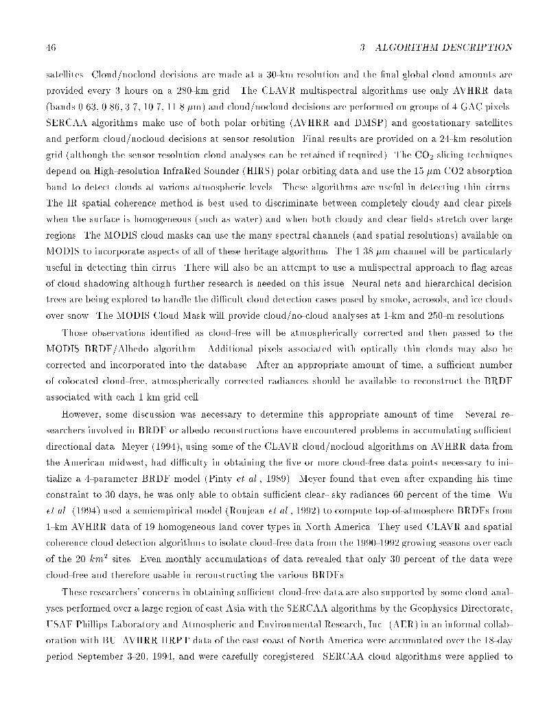
46 3 ALGORITHM DESCRIPTION
satellites. Cloud/nocloud decisions are made at a 30-km resolution and the �nal global cloud amounts are
provided every 3 hours on a 280-km grid. The CLAVR multispectral algorithms use only AVHRR data
(bands 0.63, 0.86, 3.7, 10.7, 11.8 �m) and cloud/nocloud decisions are performed on groups of 4 GAC pixels.
SERCAA algorithms make use of both polar orbiting (AVHRR and DMSP) and geostationary satellites
and perform cloud/nocloud decisions at sensor resolution. Final results are provided on a 24-km resolution
grid (although the sensor resolution cloud analyses can be retained if required). The CO2slicing techniques
depend on High-resolution InfraRed Sounder (HIRS) polar orbiting data and use the 15 �m CO2 absorption
band to detect clouds at various atmospheric levels. These algorithms are useful in detecting thin cirrus.
The IR spatial coherence method is best used to discriminate between completely cloudy and clear pixels
when the surface is homogeneous (such as water) and when both cloudy and clear �elds stretch over large
regions. The MODIS cloud masks can use the many spectral channels (and spatial resolutions) available on
MODIS to incorporate aspects of all of these heritage algorithms. The 1.38 �m channel will be particularly
useful in detecting thin cirrus. There will also be an attempt to use a mulispectral approach to ag areas
of cloud shadowing although further research is needed on this issue. Neural nets and hierarchical decision
trees are being explored to handle the di�cult cloud detection cases posed by smoke, aerosols, and ice clouds
over snow. The MODIS Cloud Mask will provide cloud/no-cloud analyses at 1-km and 250-m resolutions.
Those observations identi�ed as cloud-free will be atmospherically corrected and then passed to the
MODIS BRDF/Albedo algorithm. Additional pixels associated with optically thin clouds may also be
corrected and incorporated into the database. After an appropriate amount of time, a su�cient number
of colocated cloud-free, atmospherically corrected radiances should be available to reconstruct the BRDF
associated with each 1 km grid cell.
However, some discussion was necessary to determine this appropriate amount of time. Several re-
searchers involved in BRDF or albedo reconstructions have encountered problems in accumulating su�cient
directional data. Meyer (1994), using some of the CLAVR cloud/nocloud algorithms on AVHRR data from
the American midwest, had di�culty in obtaining the �ve or more cloud-free data points necessary to ini-
tialize a 4-parameter BRDF model (Pinty et al., 1989). Meyer found that even after expanding his time
constraint to 30 days, he was only able to obtain su�cient clear- sky radiances 60 percent of the time. Wu
et al. (1994) used a semiempirical model (Roujean et al., 1992) to compute top-of-atmosphere BRDFs from
1-km AVHRR data of 19 homogeneous land cover types in North America. They used CLAVR and spatial
coherence cloud detection algorithms to isolate cloud-free data from the 1990-1992 growing seasons over each
of the 20 km2 sites. Even monthly accumulations of data revealed that only 30 percent of the data were
cloud-free and therefore usable in reconstructing the various BRDFs.
These researchers' concerns in obtaining su�cient cloud-free data are also supported by some cloud anal-
yses performed over a large region of east Asia with the SERCAA algorithms by the Geophysics Directorate,
USAF Phillips Laboratory and Atmospheric and Environmental Research, Inc. (AER) in an informal collab-
oration with BU. AVHRR HRPT data of the east coast of North America were accumulated over the 18-day
period September 3-20, 1994, and were carefully coregistered. SERCAA cloud algorithms were applied to
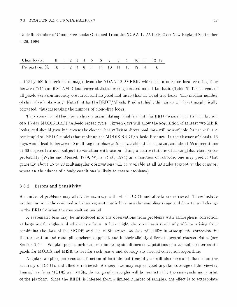
3.3 PRACTICAL CONSIDERATIONS 47
Table 6: Number of Cloud-Free Looks Obtained From the NOAA-12 AVHRR Over New England September
3{20, 1994
Clear looks: 0 1 2 3 4 5 6 7 8 9 10 11 12{18
Proportion, %: 10 1 2 4 6 11 14 10 11 15 12 4 0
a 402-by-400 km region on images from the NOAA-12 AVHRR, which has a morning local crossing time
between 7:45 and 9:30 AM. Cloud cover statistics were generated on a 1-km basis (Table 6) Ten percent of
all pixels were continuously obscured, and no pixel had more than 11 cloud-free looks. The median number
of cloud-free looks was 7. Note that for the BRDF/Albedo Product, high, thin cirrus will be atmospherically
corrected, thus increasing the number of cloud-free looks.
The experience of these researchers in accumulating cloud-free data for BRDF research led to the adoption
of a 16-day MODIS BRDF/Albedo repeat cycle. Sixteen days will allow the acquisition of at least two MISR
looks, and should greatly increase the chance that su�cient directional data will be available for use with the
semiempirical BRDF models that make up the MODIS BRDF/Albedo Product. In the absence of clouds, 16
days would lead to between 30 multiangular observations available at the equator, and about 55 observations
at 60 degrees latitude, subject to variation with season. Using a coarse statistic of mean global cloud cover
probability (Wylie and Menzel, 1989; Wylie et al., 1994) as a function of latitude, one may predict that
generally about 15 to 20 multiangular observations will be available at all latitudes (except at the equator,
where an abundance of cloudy conditions is likely to create problems).
3.3.2 Errors and Sensitivity
A number of problems may a�ect the accuracy with which BRDF and albedo are retrieved. These include
random noise in the observed re ectances; systematic bias; angular sampling range and density; and change
in the BRDF during the compositing period.
A systematic bias may be introduced into the observations from problems with atmospheric correction
at large zenith angles and adjacency e�ects. A bias might also occur as a result of problems arising from
combining the data of the MODIS and the MISR sensor, as they will di�er in atmospheric correction, in
the registration and resampling schemes applied, and in their slightly di�erent spectral characteristics (see
Section 2.6.1). We plan post-launch studies comparing simultaneous acquisitions of near-nadir center-swath
pixels for MODIS and MISR to test for such biases and develop any needed correction algorithms.
Angular sampling patterns as a function of latitude and time of year will also have an in uence on the
accuracy of BRDFs and albedos retrieved. Although we may expect good angular coverage of the viewing
hemisphere from MODIS and MISR, the range of sun angles will be restricted by the sun-synchronous orbit
of the platform. Since the BRDF is inferred from a limited number of samples, the e�ect is to extrapolate

48 3 ALGORITHM DESCRIPTION
Table 7: Estimate of Average Number of MODIS and MISR Observations Available given Cloud Cover:
Xsatview Orbital Simulation (Barnsley et al., 1994) and Cloudiness Probabilities From Wylie and Menzel
(1989) and Wylie et al. (1994).
Latitude Number of Clear-Sky Land Number of Remaining
Observations Cloud Observations
Winter Summer Prob. Winter Summer
{80 166 0 0.33 111 0
{60 54 0 0.42 31 0
{50 47 42 0.54 22 19
{40 40 36 0.63 15 13
{30 34 31 0.33 23 21
0 31 34 0.90 3 3
30 36 40 0.45 20 22
40 42 47 0.60 17 19
60 0 54 0.57 0 23
80 0 166 0.33 0 111
3.3 PRACTICAL CONSIDERATIONS 49
the BRDF to solar zenith angles where no samples were acquired. This will a�ect the accuracy of black-sky
albedo and carry over into the white-sky albedo, since the latter is the integral of black-sky albedo over all
solar zenith angles. Thus, the angular ranges sampled as well as the density of samples in that range need to
be taken into account when assessing the results of inverting the observations. The quality ags described
in Section 3.3.5 and Table 1 will give some indication of the accuracy to be expected. Note that when data
from the MODIS on the PM platform are introduced into the algorithm in the post- launch period, the
range of sun angles and azimuths will be signi�cantly expanded, thus mitigating this problem. Data from
geostationary satellites, which observe with constant view angle but changing sun angle, will be used in the
validation phase and could be incorporated into later versions of the product.
A sampling problem also arises in MODIS bands 5{7, as noted earlier in Sections 2.6.1 and 3.2.1.4. Since
MISR does not record data in these wavelengths, BRDF/Albedo inference must be based entirely on MODIS
measurements, a situation that restricts the range of available view zenith and azimuth angles. However,
model selection is based on RMS error as measured only across bands 1{4. In this way, we ensure that the
selected kernels are appropriate to the physical scattering mechanism of the cover type and are not simply
chosen by accidents of noise in bands 5{7. Since the selection of a model speci�es a type of scattering
behavior, it constrains the shape of the BRDF, and thus we expect that �tting BRDFs in these bands will
not be subject to large errors.
Yet another concern is that the BRDF and albedo of the land surface is not constant, but may be expected
to vary with time. Vegetation growth and senescence will be a major cause of BRDF/Albedo change, since
much of the scattering behavior of land surfaces is determined by the vegetation cover. Generally, vegetation
processes vary slowly and may be regarded as constant during a 16-day period. However, rapid change may
be expected at some times, as when a crop cover is harvested, or when a soil is wetted by rainfall just
prior to an observation. Another possibility is that wind e�ects on vegetation canopies will change leaf
angles su�ciently to in uence the BRDF. Rapid changes of this nature may in uence the BRDF and albedo
retrieved during a cycle, especially if one of the MISR overpasses records a surface condition di�erent from
that seen by MODIS on other days in the cycle. In such a case, we may expect that the RMSE of the
model �t will be larger, and the BRDF/Albedo value will be agged with that characteristic. It may also
be possible to detect and ag such major changes directly by such strategies as analyzing the time sequence
of near-nadir measurements from both instruments. Also, a pre-inversion outlier analysis may be used to
�lter out extreme cases.
Landscape variability, convolved with the sensor's footprint as it changes with acquisition angle, will also
add error. Although the surface cover may be quite varied at MODIS/MISR spatial resolutions of 250-m to
1.1-km, this does not present a problem for the BRDF/Albedo algorithm, since the semiempirical models are
linear BRDF combinations. That is, the BRDF of the mixed pixel will be equal to the sum of the BRDFs
of the di�erent cover types within it as weighted by their relative areas, provided that adjacency e�ects may
be ignored. This property is also important for degrading BRDF and albedo to spatial resolutions of less
than 1.1 km when required, as for example for global climate modeling at 0.5� resolution.

50 3 ALGORITHM DESCRIPTION
However, scene heterogeneity is partly a function of resolution cell size. Given the larger projected IFOV
of MODIS at extreme o�-nadir angles, the e�ect will vary in magnitude across the instrument scan line.
As a result, spatial autocorrelation will increase and we may also expect that angular samples obtained at
extreme view angles will also be more highly correlated. One possible impact of this may be to smooth the
apparent BRDF at extreme view angles by reducing the spatial variance in detected radiance (Barnsley and
Kay, 1990). However, the product will be derived from MODIS bands with 250- and 500-m spatial resolution
that are gridded 1-km; similarly, the MISR product will be derived from collapsing 275-m spatial resolution
data to 1.1 km. These data characteristics will reduce the e�ect to an important degree. Some aspects of
spatial scaling a brie y discussed in Appendix F.
A related e�ect is misregistration noise, in which the geolocation of an observation contains errors. If
the errors are random and unbiased, then the e�ect will be to enlarge the e�ective footprint of the detector
and smooth the BRDF. Note that extensive e�orts will be made by both MODIS and MISR teams to reduce
biases in geolocation using postlaunch characterization of instrument performance. Other than reducing
the spatial resolution of the product, there is little that can be done to correct for the e�ects of errors in
registration.
In order to accommodate noise, bias and sampling e�ects, we note that the inversion algorithm attributes
individual weights to each observation. This allows us to lessen the impact of problematic data points by
reducing their weight, rather than simply eliminating them. We may want to use some of the information in
problematic points, especially if they were acquired in an angular range that is otherwise not well sampled.
Another factor in uencing the quality of the product is data availability. The MISR Level 2 surface
product will be phased in during the �rst �ve quarters following launch, so that in the immediate post-
launch period, the BRDF/Albedo product will be derived only from MODIS data for many parts of the
world. As the sixth quarter approaches, successively more area will be covered by the MISR product until
land and tropical ocean coverage is complete. Quality ags will indicate when the BRDF/Albedo product
is made for a grid cell without MISR data (see Table 1).
The issues of noise, bias and sampling need to be addressed systematically as part of the development of
the product. The following two sections, as well as Appendices B and C which give greater detail, discuss
the two most important of these e�ects: the in uence of noise-like e�ects in the re ectances and the e�ect
of changing and limited angular sampling on BRDF and albedo retrievals.
3.3.2.1 Retrieval Accuracies of BRDF and Albedo from MODIS and MISR Angular Sam-
pling
Note: A full detailed report on the retrieval accuracies from MODIS and MISR angular sampling using the
kernel-driven Ambrals semiempirical BRDF model is given in Appendix B. Please refer to this appendix for
tables, �gures and an in-depth discussion.
A study was carried out to determine the e�ects of the particular angular sampling available from
MODIS and MISR on BRDF and albedo retrievals, and the e�ects of seasonal and latitudinal changes in

3.3 PRACTICAL CONSIDERATIONS 51
Table 8: Summary of Median Predicted Retrieval Accuracies at the Mean Sun Zenith Angle of Observation:
All Latitudes, Times of Year, Biome Types.
Model Albedo Nadir Re ectance
Ambrals 3.1 (0.5{9.6) 3.3 (0.7{8.1)
mod. RPV 3.2 (0.4{8.3) 2.7 (0.9{8.8)
mod. Walthall 5.0 (1.1{11.8) 14.5 (2.3{35.8)
that sampling on these parameters. Since the exact distribution of angular sampling is important for a study
as this, and observed BRDFs are not sampled in a corresponding manner nor are available in conjunction
with ground truth, the only way to conduct such a study is to use a complex numerical forward model to
simulate observations and then use a simpler inversion BRDF model to invert them and derive quantities of
interest. A comparison of this sort, model against model, clearly has its drawbacks, as problems found could
be due to either model. For example, if the inversion model has problems �tting the BRDF at large zenith
angles, the problem could be due to unrealistic behavior at large zenith angles in either model. Still, in the
absence of real MODIS and MISR data this method is the best available to reach some understanding of the
accuracy to be expected from MODIS and MISR BRDF and albedo retrievals given their speci�c angular
sampling geometries.
The study was conducted as follows. The orbital simulation tool Xsatview (Barnsley et al., 1994) was
used to generate simulated MODIS and MISR viewing and illumination geometries for geographic latitudes
of observation between 80 degrees south and 80 degrees north, and for 8 di�erent 16-day time periods
throughout days of the year. For each of the observation geometries generated, a discrete ordinates method
radiative transfer code (Myneni et al., 1992) was used to compute simulated observations of the bidirectional
surface re ectance for six distinct BRDF types resembling six di�erent land cover types in the red and the
near-infrared (NIR) wavebands. These types were grasslands, semi-arid shrublands, broadleaf crops, savanna,
broadleaf and needleleaf forests.
The resulting re ectances were then inverted using the Ambrals kernel-driven BRDF model. For com-
parison, the modi�ed RPV BRDF model (Rahman et al., 1993b; Engelsen et al., 1996) and the empirical
modi�ed Walthall model (Walthall et al., 1985; Nilson and Kuusk, 1989) were also inverted.
The accuracy and variation with which the following parameters were derived was investigated: nadir-
view re ectance and black-ksy albedo at the mean sun angle of observation ("interpolation"); nadir-view
(actually, 10 degree zenith angle to avoid the hotspot) re ectance and black-sky albedo at nadir sun angle;
and white-sky albedo.

52 3 ALGORITHM DESCRIPTION
Table 9: Summary of Predicted Retrieval Accuracies: All Latitudes, Times of Year, Biome Types and Solar
Zenith Angles, Irrespective of the Solar Zenith Angle of Observation. Median and Two-Thirds of Cases
Range, the Ranges Being With Respect to Solar Zenith Angle.
Model Albedo Nadir Re ectance
Ambrals 2.0{8.1 (0.5{16.0) 3.2{7.9 (0.7{28.7)
mod. RPV 2.5{7.9 (0.4{15.4) 2.3{10.3 (0.9{28.2)
mod. Walthall 3.5{26.5 (1.1{48.6) 8.7{19.0 (2.0{55.6)
Table 10: Summary of Predicted Retrieval Accuracies as a Function of Cloud Probability: All Latitudes,
Biome Types and Solar Zenith Angles for a 16-Day Time Period Beginning Day of Year 96. Median and
Two-Thirds of Cases Range, the Ranges Being With Respect to Solar Zenith Angle.
Prob. of Cloud Albedo Nadir Re ectance
0 % 2.0{7.8 (0.7{18.4) 3.2{9.2 (0.4{31.4)
25% 1.9{8.0 (0.8{17.9) 3.2{9.0 (0.5{30.8)
50 % 2.3{8.1 (0.7{18.6) 3.1{9.2 (0.7{31.2)
75 % 3.1{9.0 (0.7{18.7) 2.6{9.3 (0.7{29.6)

3.3 PRACTICAL CONSIDERATIONS 53
In a �rst step, accuracies possible if no observations are lost to clouds were derived. These are the
bottom-line accuracies that allow studying how additional e�ects lead to an increase of error. Table 8
summarizes error across band for retrievals at the mean sun angle of observation. The numbers given refer
to the median (typical) relative error made and the range of relative errors typically found between good
and bad retrievals. The Ambrals and the modi�ed RPV BRDF models perform similarly well, with median
accuracies of albedo and re ectance retrievals of only a few percent (less than 10 percent even in typical bad
cases); but the modi�ed Walthall model shows larger errors due to its empirical nature. This shows that
the semiempirical models retain some of their physical properties despite the severe approximations made in
deriving them. The modi�ed Walthall model is attractive only because of its great mathematical simplicity,
which is attractive to some applications where accuracy requirements are less strict.
Table 9 shows results for a more severe test. It gives median expected errors for retrievals not only at the
mean sun angle of observation but at other sun angles (0, 30 and 60 degrees) as well, testing extrapolation of
the derived parameters away from the angles of observation. The numbers given refer to the median (typical)
relative error made, the range being with respect to variations in the sun zenith angle of prediction, and the
range of relative errors typically found between good and bad retrievals. Despite the severity of the test,
one may see that both nadir-view re ectance are retrieved to within 10 percent at all sun zenith angles,
irrespective of the angle of observation. Again results for the modi�ed RPV model are very similar, but
those for the modi�ed Walthall model are clearly inferior, with median errors of up to 25 percent found at
some sun angles.
Table 10 determines whether these accuracies are expected to strongly deteriorate as observations are
lost to cloud cover. It shows that this is not the case even if 75 percent of observations are (randomly)
lost. This is true if loss is such that the angular sampling patterns gets sparser, but good angle coverage
is retained. Retrievals are expected to still be approximately accurate in line with Tables 8 and 9 in the
presence of clouds.
Please refer to Appendix B for a full report of this retrieval accuracy study, including tables, �gures and
more detailed analysis.
3.3.2.2 Sensitivity of MODIS and MISR BRDF and Albedo Retrieval to Noisy Data
Note: A full detailed report on the noise sensitivity of the kernel-driven Ambrals semiempirical BRDF model
for MODIS and MISR angular sampling is given in Appendix C. Please refer to this appendix for tables,
�gures and an in-depth discussion.
Actual measurements of surface re ectance will always include a certain amount of noise, which may
be random, systematic, or a combination of both. Such noise will result in error in retrievals of BRDF
parameters and albedo. A key criterion to assess the validity of the retrieval process is to verify that it does
not amplify the noise-like errors associated with individual measurements of surface re ectance. In order to
investigate this problem, a full noise sensitivity study was conducted for the Ambrals BRDF model.
The behavior of kernel-driven BRDF models under the conditions of varying angular sampling and noisy

54 3 ALGORITHM DESCRIPTION
data can be studied analytically due to the mathematical form of these models. It is given by the the
so-called \weights of determination", calculated using theory that originates with Gauss (Whittaker and
Robinson, 1960). Kernel-driven models give the re ectance R in form of a sum, R =Pfiki, where fi are the
model parameters and ki are mathematical functions (\kernels") giving basic BRDF shapes depending only
on sampling geometry. The expected error in a term u given by a linear combination of model parameters,
u =PfiUi (e.g., R itself at a given combination of angles, or integrals of the BRDF such as directional
and di�use albedo), is given by �u = e=pwu, where e is the estimate of standard error in the observed data
(approximated by the RMSE in model �tting), and 1=wu is the weight of determination of term u under the
sampling considered. This weight is given through 1=wu = [U ]T [M�1][U ], where U is a vector composed of
the terms Ui and M�1 is the inverse matrix providing the analytical solution to the problem of inverting a
set of re ectances Ri for model parameters fi minimizing a given error function. Note that this analysis is
independent of any speci�c BRDF function.
In our investigation, we have studied the sensitivity to random noise of all kernel combinations that
comprise the Ambrals BRDF model using sampling for a variety of combinations of the MODIS and MISR
sensors, and for di�erent periods of data accumulation. From these, we here report selected �ndings on
16-day sampling only for 3 di�erent sensor combinations. Both interpolating and extrapolating the BRDF
were tested in that nadir re ectance and directional-hemispherical (\black-sky") albedo were derived both
at the mean sun angle of the observation and for nadir sun. Additionally, bihemispherical (\white-sky")
albedo and the model parameters themselves were investigated.
Table 11 summarizes �ndings. The base case studied was 16-day sampling for combined MODIS and
MISR data, as for the MODIS BRDF/albedo product. We further investigate whether using MODIS data
alone is an option, and whether a second MODIS sensor to be launched on the EOS-PM-1 platform is a
potential substitute for MISR in view of the three additional bands that MODIS has over MISR. Table 11
lists �rst the median weights of determination found for sampling throughout the year and at all latitudes.
Given are the values found for the BRDF model with the smallest and with the largest median weight.
Second, it gives the worst-case range of values. Range here is de�ned as the central two thirds of values
occurring.
Results show that the MODIS-AM/MISR sensor combination will allow retrieval of the BRDF with
an accuracy that is smaller than the RMSE of the inversions (weights if determination smaller than one).
Retrieval of nadir re ectance and black-sky albedo at the mean prevailing sun zenith angle is very stable
and more reliable than deriving these quantities for a nadir sun. But even the latter, requiring extrapolation
of the BRDF to angles where typically no observations were made, is possible with an accuracy of less
than the value of the RMSE. The same is true for the white-sky albedo. The expected error of the model
parameters themselves is larger than that of derived quantities. Naturally, cloud cover will increase these
error estimates. Assuming that the angular distribution of samples is not a�ected by loss of observations
due to clouds, the weights of determination can be shown to increase as 1=pN , where N is the number of
observations.
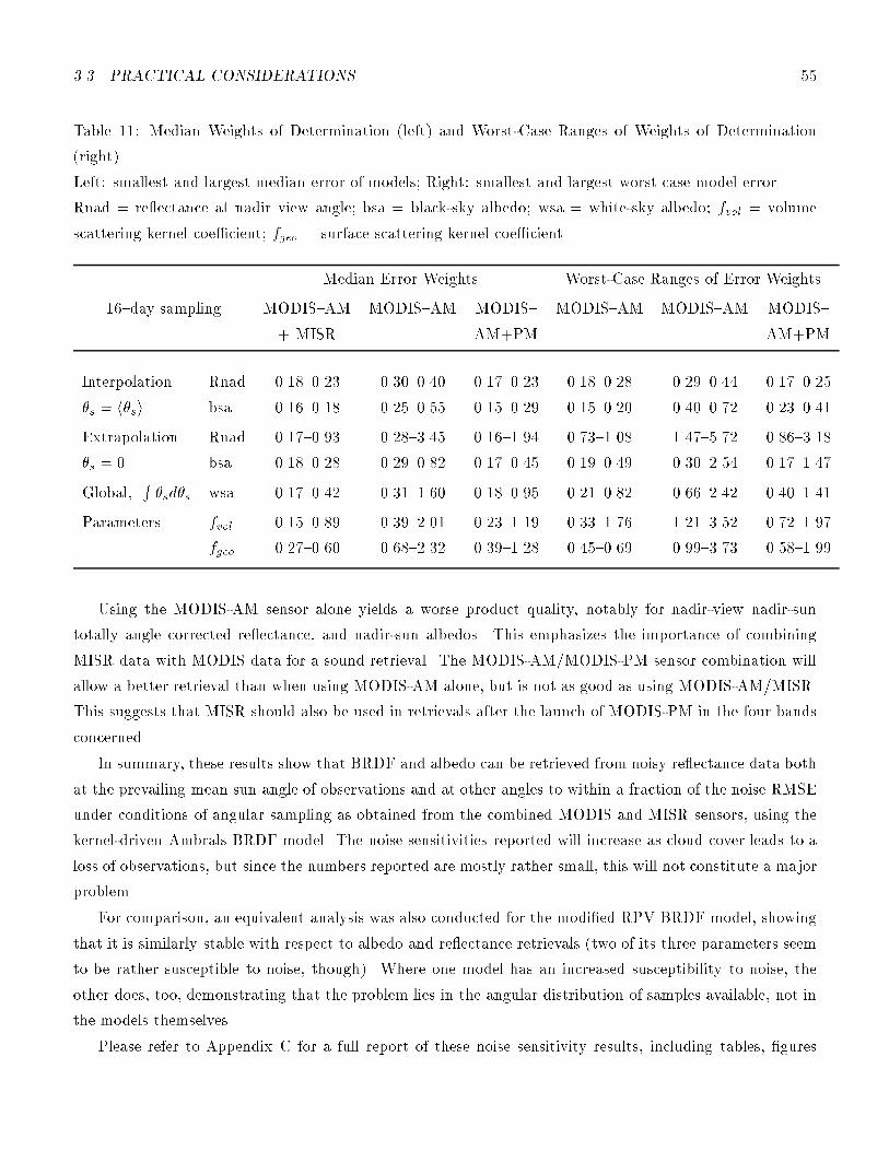
3.3 PRACTICAL CONSIDERATIONS 55
Table 11: Median Weights of Determination (left) and Worst-Case Ranges of Weights of Determination
(right).
Left: smallest and largest median error of models; Right: smallest and largest worst case model error.
Rnad = re ectance at nadir view angle; bsa = black-sky albedo; wsa = white-sky albedo; fvol = volume
scattering kernel coe�cient; fgeo = surface scattering kernel coe�cient.
Median Error Weights Worst-Case Ranges of Error Weights
16{day sampling MODIS{AM MODIS{AM MODIS{ MODIS{AM MODIS{AM MODIS{
+ MISR AM+PM AM+PM
Interpolation Rnad 0.18{0.23 0.30{0.40 0.17{0.23 0.18{0.28 0.29{0.44 0.17{0.25
�s = h�si bsa 0.16{0.18 0.25{0.55 0.15{0.29 0.15{0.20 0.40{0.72 0.23{0.41
Extrapolation Rnad 0.17{0.93 0.28{3.45 0.16{1.94 0.73{1.08 1.47{5.72 0.86{3.18
�s = 0 bsa 0.18{0.28 0.29{0.82 0.17{0.45 0.19{0.49 0.30{2.54 0.17{1.47
Global,R�sd�s wsa 0.17{0.42 0.31{1.60 0.18{0.95 0.21{0.82 0.66{2.42 0.40{1.41
Parameters fvol 0.15{0.89 0.39{2.01 0.23{1.19 0.33{1.76 1.21{3.52 0.72{1.97
fgeo 0.27{0.60 0.68{2.32 0.39{1.28 0.45{0.69 0.99{3.73 0.58{1.99
Using the MODIS-AM sensor alone yields a worse product quality, notably for nadir-view nadir-sun
totally angle corrected re ectance, and nadir-sun albedos. This emphasizes the importance of combining
MISR data with MODIS data for a sound retrieval. The MODIS-AM/MODIS-PM sensor combination will
allow a better retrieval than when using MODIS-AM alone, but is not as good as using MODIS-AM/MISR.
This suggests that MISR should also be used in retrievals after the launch of MODIS-PM in the four bands
concerned.
In summary, these results show that BRDF and albedo can be retrieved from noisy re ectance data both
at the prevailing mean sun angle of observations and at other angles to within a fraction of the noise RMSE
under conditions of angular sampling as obtained from the combined MODIS and MISR sensors, using the
kernel-driven Ambrals BRDF model. The noise sensitivities reported will increase as cloud cover leads to a
loss of observations, but since the numbers reported are mostly rather small, this will not constitute a major
problem.
For comparison, an equivalent analysis was also conducted for the modi�ed RPV BRDF model, showing
that it is similarly stable with respect to albedo and re ectance retrievals (two of its three parameters seem
to be rather susceptible to noise, though). Where one model has an increased susceptibility to noise, the
other does, too, demonstrating that the problem lies in the angular distribution of samples available, not in
the models themselves.
Please refer to Appendix C for a full report of these noise sensitivity results, including tables, �gures
56 3 ALGORITHM DESCRIPTION
and more detailed analysis.
3.3.3 Numerical Computation Considerations
On the computational side, the two issues of interest are requirements in computing power and storage size
of the output product. No special requirement is foreseen for the memory required for execution of the
algorithm.
Timing was conducted on the version 1 software delivered in the summer of 1996 at SDST. There are two
processes currently being delivered for the BRDF/Albedo product. One is the multiangular 1-km re ectances
database building process (MOD43B1) which serves several other products besides BRDF/Albedo and is
in itself not strictly related to BRDF and albedo retrieval. Running on the SDST-supplied synthetic data
set, scaled for latitudinal variations in the number of observations occurring, and including a 4/7 share of
processing for MISR data, this process is currently estimated to require 400 MFlop/s of computing power.
The actual BRDF and albedo process (MOD43B2) was timed not using the synthetic data set but a
more realistic SCF-produced data set. This set was more realistic in that it contained a BRDF (which
the SDST-provided synthetic data set does not) and it was scaled to re ect typical average numbers of
observations. The process is currently estimated to require 300 MFlops/s of computing power.
These numbers were derived using SDST-provided assumptions and following SDST's computing outline.
Increases in speed are possible for the version 2 code but hard to quantify at present.
The size of the BRDF/Albedo Product is found to be 33.1 GByte in 16 days or 2.1 GByte per day, each
subdivided into sets of 355 tiles, for land only.
3.3.4 Calibration and Validation
The prelaunch e�orts to validate the BRDF/Albedo Product emphasize: (1) a validation of the ability
of the semiempirical models to �t observed measurements of bidirectional re ectance, and by integration,
albedos; and (2) a validation of the ability of the algorithm to process data acquired over large regions in an
appropriate and e�cient fashion. In the postlaunch era, validation e�orts will focus on a comparison of the
BRDFs and albedos produced by the operating algorithm with the actual measurements acquired during
the initial period of product compilation.
All of these e�orts rely on the availability of diverse, well characterized test sites with su�cient ground
instrumentation to accumulate comprehensive validation data sets. The MODLAND products teams are
embracing the EOS test site �ve-tiered hierarchy of (1) Intensive Field Campaigns (such as Boreas and
LBA); (2) Fully Instrumented Long Term Super Sites (such as the ARM/CART sites); (3) Biome Tower
Sites (networks of long term instrumented sites such as LTER); (4) Globally Distributed Test Sites (min-
imally instrumented permanent sites widely distributed over the globe such as SURFRAD or the NOAA
CMDL Flask Network); and (5) Instrument Calibration Sites (such as White Sands). While individual team
scientists are involved in all the recent and planned Intensive Field Campaigns, and at the ARM/CART

3.3 PRACTICAL CONSIDERATIONS 57
sites, White Sands or Railroad Playa, the MODLAND team is specially focusing on the development, char-
acterization and instrumentation of the Tier 3 and 4 sites. The current plan is to have 10 Tower Sites
in place prelaunch and add 10 more soon after launch with as many as 60 operating worldwide eventu-
ally. Quantities to be observed for radiometric validation are the following: (1) atmospheric properties
(aerosol optical thickness and properties, water vapor, ozone); (2) irradiance characteristics (downwelling
irradiance total and angular distribution); (3) re ectance characteristics (land surface BRDF, directional-
hemispherical re ectance and bihemispherical re ectance); (4) land surface properties (land surface/canopy
type and major structural characteristics, current seasonal state, LAI, leaf re ectance, soil brightness and
type). The instrument package (CIMEL multi-directional sunphotometer, pyranometer, pyrgeometer, gas
ux instrumentation, and basic meteorological instrumentation) and temporal and spatial sampling plans
will be prototyped at two existing research sites (the SALSA site and the Oak Ridge site) in the summer of
1997.
In addition to ground measurements from these Tier 3 Tower Sites or from Tier 2 Intensive Field Cam-
paigns, the BRDF/ALbedo Product validation e�ort will rely extensively on laboratory measurements,
modeling exercises, and data from multidirectional aircraft and space based sensors.
3.3.4.1 Validation of Model Fit. Future validation of the ability of semiempirical models to �t ob-
served data involves laboratory, �eld, and aircraft measurements. In the laboratory, data from two ongoing
research programs are of particular interest. The �rst program involves a collaboration between Boston
University and the Chinese Academy of Science. As a part of this program, data were acquired under our
direction at a unique Chinese facility-the Solar Simulation Laboratory of the Jingyuetan Remote Sensing
Test Site, Changchun, China (Strahler and Liang, 1994). In this laboratory, we illuminated several target
plant canopies of 1 m2 extent with a parallel beam from an arc lamp providing near-solar illumination
conditions. A semicircular framework, moving in a circular target around the track, supported radiometers
acquiring measurements at 10� increments of view zenith and azimuth in Thematic Mapper Bands 1{4.
Solar zenith angle was variable between 0� and 45�. Data acquired in 1994 and 1995 included canopies
of soybean, nasturtium, and other plants as well as bare soil. Because these data were acquired without
signi�cant di�use illumination, they do not require atmospheric correction. The data are currently in the
analysis phase, and early indications are that the semiempirical models �t the observations very closely
(Strahler et al., 1996). More data acquisitions are planned for 1997.
A second set of laboratory data that is being used to test the �t of the semiempirical models to re ectance
measurements has been acquired by J. Miller at York University { multiband, multiangular measurements of
re ectance of an arti�cial conifer canopy acquired by the Compact Airborne Spectrographic Imager (CASI)
instrument (Babey and So�er, 1992). The canopy consists of model trees designed to simulate the physical
shape and structure of individual conifer crowns (So�er and Miller, 1995). They are sprayed with cellulose
material that emulates the spectral response of leaf tissue, and are arranged according to �eld measurements
of real conifer stands. This laboratory setup allows a systematic exploration of the in uence of background

58 3 ALGORITHM DESCRIPTION
brightness, tree density, and solar zenith angle on the BRDF in a way that is not possible in a �eld campaign.
In tests involving a random spatial distribution of trees and a spatial pattern resembling the BOREAS Jack
Pine site, the semiempirical models have �t the data quite well.
In addition to these direct laboratory measurements, numerical simulation studies using the Monte Carlo
ray-tracing system (Lewis and Muller, 1992) and Botanical Plant Modelling System (Lewis, 1990; Lewis et
al., 1991) will be used at UCL to simulate directional re ectance measured by instruments with an equivalent
pixel IFoV of 3m at the vegetation canopy level. (see section 3.1.4.2 for more details as well as Appendix H).
This e�ort is providing a full simulation of all the characteristics a�ecting the BRDF and albedo under
controlled conditions. In particular, the in uence of the BRDF of plant components (such as leaves) and the
soil on the canopy-level BRDF can be studied. This e�ort will also aid in understanding how semiempirical
BRDF parameters may be interpreted in a physical sense and whether any of the parameters, such as LAI,
have any physical signi�cance. Simulation of datasets for HAPEX-Sahel are the primary focus of the work
at present.
Another source of model validation data exists in ground measurements of surface radiance as a function
of view and illumination positions. Such data are usually expressed as bidirectional re ectance factors
(BRFs) and include the e�ects of di�use (sky) irradiance of the target. However, there is no barrier to �tting
these data to semiempirical models as long as it is noted that the functions describe BRF observations rather
than true BRDFs. In such cases, the presence of skylight will smooth the BRDF shape to some degree.
Thus far, we have �t semiempirical models to over 27 sets of observations with very good results (see
Section 3.1.4.1 and Appendix A). These include the classic datasets of Ranson et al. (1985), Kriebel (1978)
among others. In addition, a considerable archive of angular surface re ectance data acquired by D. Deering
with the PARABOLA instrument was been tested. There are also plans to collocate PAROBOLA with the
CIMEL directional sun photometer during the Tier 3 Tower Site prototype exercise in the summer of 1997.
It is hoped that a downward pointing scanning CIMEL photometer will adequately characterize the BRDF
in the vicinity of the tower in an automated fashion and provide a valuable source of pre and post launch
validation data.
As part of the ongoing collaboration between the Boston University Center for Remote Sensing and the
Chinese Academy of Science (CAS) Institute of Remote Sensing Application (IRSA), we will also acquire
�eld data from an agricultural experiment station located at Yucheng, Shandong Province, China. Instead
of multiangle measurements made during a short time period, we will observe crop re ectance from a �xed
position on a nearby tower as sun angle changes during the day. In this way, we will observe the day-to-day
variability of directional re ectance as environmental and crop conditions change.
Aircraft acquisitions are a further source of directional re ectance data. The principal source of such
data is the ASAS (Advanced Silicon Array Spectrometer) instrument (Irons et al., 1991), which acquires �ne
spatial resolution multispectral measurements at view zenith angles from +75� (forward) to �60� (aft) in
the ight direction. Typically, observations are made along the principal plane, across the principal plane,
and at an azimuth angle of 45� to the principal plane. Most ASAS data are of homogeneous targets and
3.3 PRACTICAL CONSIDERATIONS 59
are accompanied by measurements characterizing aerosol properties and optical depth, allowing testing of
the BRDF-atmospheric correction loop (see Section 3.2.4). Among the investigators on the BRDF/Albedo
team, we already have about a dozen ASAS datasets that may be used for validation.
ASAS data from the Hapex-Sahel has been processed at UCL to remove geometric distortions due to
aircraft motion (Allison et al., 1991; Allison and Muller, 1992; Allison et al., 1994). Unfortunately, the C-130
aerial photographs taken at the same time as the ASAS imagery were not taken with su�cient stereo overlap
to create detailed DEMs and orthoimages and no GPS-based control has been able to be acquired from HSIS
for geocoding of the aerial photographs using a 30m DEM created using ERS tandem SAR interferometry.
However, using the 6S simulation system (Vermote et al., 1994) and in situ atmospheric optical depth mea-
surements from Halthore (Brown de Coulstoun et al., 1996) , it was possible to atmospherically correct the
data (see Section 3.1.5.2). Barnsley et al. (1996) describe how multiple ight-lines of ASAS processed data
over the HAPEX- Sahel southern super-site were used to retrieve empirical (Walthall) BRDF distributions
at 3m resolution using the aforementioned methods (see Appendix J). Work has been completed at UCL to
process the entire HAPEX-Sahel dataset (18 ight-lines over 3 sites) into "at surface" re ectance". These
registered re ectance maps have been used to invert "ambrals" and for two models (modi�ed Walthall
and RossThick-LiSparse) have been used to derive spectral BRDFs and spectral albedos for a complete
LANDSAT-TM scene (see section 3.1.5.2 and Appendix G). The derived albedos, once integrated over the
shortwave region, will be compared with in situ measurements acquired by solarimeters (Allen et al., 1994).
Work is also underway at UCL to extend these studies to other ASAS ight-lines, where the other necessary
datasets (e.g., atmospheric optical depth measurements, aerial photographs, DEMs) are available.
In addition to this work, similar inversions will also be made at UCL with atmospherically-corrected
airborne POLDER data over HAPEX-SAHEL (Roujean et al., 1996) and BOREAS (Bicheron et al., 1996;
Breon et al., 1996) and results compared with those from ASAS (see Section 2.6 for more detail on the
POLDER instrument). POLDER simulator data are also available for the La Crau test site in southern and
for BOREAS (V. Vanderbilt, personal communication). At present, the La Crau data are being �tted to
semiempirical models at CAS-IRSA under the direction of X. Li, a member of the POLDER Science Team
who is also a member of the BRDF/Albedo product team.
A similar airborne instrument belonging to the Chinese Academy of Science acquired data from the
Changping region, near Beijing, in the fall of 1995. These data sets are currently being analyzed.
J. Miller of York University has also indicated interest in �tting the semiempirical models to airborne
CASI data acquired during BOREAS from stands of old jack pine, with and without a ground cover of snow
(J. Miller, personal communication).
An excellent source of future airborne measurements will be provided by the AirMISR which will be-
gin acquiring data early in 1997. Several of the sites initially scheduled for over ights will also supply
PARABOLA data thereby generating very interesting BRDF validation data sets. Coordination is under-
way between MODLAND and MISR to schedule several over ights of the intitial Tier 3 MODIS Biome
Tower sites early in 1998.

60 3 ALGORITHM DESCRIPTION
3.3.4.2 Large-Area Application In addition to validation of the ability of the semiempirical models
to describe BRDFs and infer albedos, there is a need to apply the BRDF/Albedo algorithm to MODIS-like
data from large areas to validate the operational aspects of the algorithm. The most suitable data for this
purpose are AVHRR LAC data, since the AVHRR has a view geometry and pixel size in LAC mode similar
to that of MODIS, although the orbital crossing times are somewhat di�erent.
As described in Section 3.3.1, AVHRR LAC data from the east coast of North America are currently
being accumulated by the Geophysics Directorate of the USAF Phillips Laboratory and Atmospheric and
Environmental Research, Inc., in an informal collaboration with Boston University. The primary objective
is to characterize the BRDF of the surface as an aid to cloud detection for use in cloud characterization
algorithms. In addition to providing information on the availability of cloud-free surface observations, the
study will exercise the BRDF/Albedo algorithm over a large region through time. Although there are
no supporting ground truth data for BRDF or albedo for direct validation, we can nonetheless check for
reasonable results. The study will help us both to understand better operational problems and constraints,
and to estimate processing times more accurately.
A similar AVHRR LAC dataset is also being accumulated in China for a 54,000 km2 region incorporating
the area expected to be ooded following the completion of the Three Gorges Dam on the Yangtse River.
Data acquisition, which started in early 1995, is supported by the National Science Foundation of China
and the CAS Institute of Remote Sensing Applications under a grant with X. Li as Principal Investigator.
As part of the project, ground truth measurements will be acquired that can be used to test BRDF/Albedo
retrievals directly. Dr. Li is also a member of the SPOT-VEGETATION team, with an approved proposal
to use SPOT-VEGETATION data for environmental surveillance of the Three Gorges Dam region. Thus,
we may be able to use SPOT-VEGETATION data in validation as well (see Section 3.3.4.3).
In yet another AVHRR application, D. Meyer at the EROS Data Center is applying semiempirical models
to AVHRR LAC data for a transitional region in the northern midwest that exhibits a range of vegetation
covers. The study will focus on albedo retrieval and model selection for the various cover types. Some
ground validation data will also be acquired (D. Meyer, personal communication).
GAC data from the AVHRR Path�nder dataset can also serve as a source for testing large-scale appli-
cation of the BRDF/Albedo algorithm. However, this application is limited by the subsampling pattern of
the instrument in GAC mode, as well as by problems of geometric accuracy and atmospheric correction.
Data from the ADEOS borne POLDER instrument is also very useful in validating the BRDF/Albedo
algorithm. Since it acquires successive overlapping images of the ground along the orbital path, it is closer to
MISR in its imaging characteristics than to MODIS. The instrument is discussed in more detail in Section 2.6.
It provides the opportunity to apply the BRDF/Albedo algorithm in an operational context and also allow
some measure of validation with ground truth. This e�ort is supported by X. Li and M. Barnsley, members
of the POLDER Science Team who are also a members of the MODIS BRDF/Albedo team, as well as M.
Leroy, who is heading the POLDER surface re ectance-BRDF e�ort. Test sites for acquisition of POLDER
data range from La Crau, FIFE and BOREAS sites to the previously mentioned Changping and Yucheng

3.3 PRACTICAL CONSIDERATIONS 61
sites in China.
3.3.4.3 Postlaunch Validation During the postlaunch validation phase, emphasis will be placed on
comparing the BRDF/Albedo Product with (1) ground data at the Tier 3 and 4 EOS Test Sites; (2) ground
data from Tier 2 sites-of-opportunity in connection with future multidisciplinary �eld experiments (e.g.,
FIFE, BOREAS, LBA); (3) MISR surface re ectance, BRDF and albedo products; (4) POLDER surface
re ectance, BRDF and albedo products; and (5) possible BRDF/Albedo products from AVHRR Path�nder.
The MISR instrument is colocated with MODIS on the AM platform and, although the MISR surface
re ectance data are used in the MODIS BRDF/Albedo Product, the single instrument products can also
serve as a source of validation. The MISR Surface Product depends on the Rahman{Pinty{Verstraete model
(RPV) (Rahman et al.,1993) in a form modi�ed by Martonchik (Englesen et al., 1996) to supply BRDF and
albedo parameters (Diner et al., 1996; Maronchik, 1997). As shown by Wanner (see Appendix B), either
the RPV or the Ambrals models retrieve these parameters with reasonable accuracy. Postlaunch validation
will therefore include a component of comparison to highlight the similarities and di�erences between these
products and address the e�ects of di�erence atmospheric correction schemes, temporal variation and spectral
coverage.
Other satellite-based postlaunch validation opportunities concern the SPOT{VEGETATION instrument
and the meteorological satellites. SPOT{VEGETATION, due for launch several months after the AM
platform, is a wide-�eld, three-band (blue, red, near-infrared) pushbroom instrument with a 1-km spatial
resolution. It di�ers from the AVHRR primarily in its blue band and in the fact that its spatial resolution,
by virtue of the pushbroom design, will be constant in the across-track direction. At this time, the SPOT{
VEGETATION science plan is still under development, and we are not certain which products will be most
useful for validation.
Current and future GOES US geostationary meteorological satellites have improved, onboard, visible
radiometric calibration (not available before GOES-8) and �ner 10-bit (vs. older 8-bit for pre-GOES-8)
radiometric resolution at a nominal 1-km spatial resolution. With these characteristics, spatially coincident
geostationary and polar orbiting data may be helpful in validation of the BRDF/Albedo product. In contrast
to MODIS/MISR, in which view angle and azimuth vary freely while sun position is constrained by latitude
and the platform crossing time, geostationary satellites hold view position constant through the day, while
sun position changes throughout the full diurnal cycle. Given auxiliary data on the atmospheric state
throughout the day covering the MODIS swath, it will be possible to compare the exoatmospheric radiance
directional re ectance for any given area based on the MODIS/MISR BRDF at a variety of di�erent solar
angles with the exoatmospheric radiance available from GOES. Eventually with MODIS-PM data it may be
possible to improve the accuracy of the BRDF extrapolation to other solar angles (van Leeuwen et al., 1996).
In addition, it may eventually be possible to integrate GOES-derived "at-surface" directional re ectance to
provide for diurnal cycles of albedo which are required by hydrologists.
Arino et al. (1991, 1992) and Dedieu (1992) provide an approach to validation for AVHRR with ME-
62 3 ALGORITHM DESCRIPTION
TEOSAT that may be useful for the BRDF/Albedo product in the postlaunch period. In this method,
geostationary satellite exoatmospheric radiance is predicted using the surface BRDF and the derived atmo-
spheric parameters, assuming a constant atmosphere for the time interval under study. The GOES-Next
series of satellites will be particularly relevant for this purpose, although their spectral bands are much
broader than MODIS. At-satellite radiance is predicted using atmospheric codes such as 6S (Vermote et al.,
1994). If the terrain is suitably rugged (see discussion in Section 3.2.6), the simulation may also need to take
into account mutual illumination e�ects. Monte Carlo ray-tracing (Lewis and Muller, 1992; Muller and Dal-
ton, 1988) can then be used to represent these multiple scattering events. However, the large computational
requirements of ray tracing will probably restrict its use to a few well-de�ned EOS test sites.
Polar orbiting instruments, such as SCARAB and CERES, which will be on multiple platforms, will also
provide the opportunity to validate BRDF/Albedo in the context of the global radiation budget. CERES will
provide shortwave albedo from the same platform as MODIS. However, the coarser resolution of CERES
and the greater likelihood that partial �elds-of-view will be cloud-covered pose some obstacles to direct
comparisons with the CERES albedos with the BRDF/Albedo product.
In addition to these directly sensed measurements, the BRDF/Albedo product can be validated by com-
parisons with existing coarse-resolution global albedo databases. These range from static parameterizations
based on land cover (such as the ISLSCP Initiative I and II products for albedo) to satellite-based obser-
vations in broad and narrow bands by METEOSAT and, in the past, by ERBE (Earth Radiation Budget
Experiment). Li and Garand (1994) enumerate these datasets more fully. For BRDF, the scene- dependent
top-of-atmosphere angular re ectance models of ERBE (Barkstrom and Smith, 1986; Taylor and Stowe,
1984) are an obvious point of comparison, although the footprint of ERBE radiometers is about 40 km at
nadir. A comparison with these coarse resolution databases will be facilitated by the use of linear semiempir-
ical models of BRDF/Albedo, which can be easily aggregated to coarse resolutions for quantitative overlays
to alternative datasets.
3.3.5 Quality Control and Diagnostics
MODIS standard data products are comprised of science data sets and metadata. The EOSDIS Core System
(ECS) architecture provides for the storage of QA results in both the metadata and in the science data sets.
Mandatory ECS QA ags are stored in the core metadata. These mandatory ags include QA statistics and
text that summarize the application of runtime or post run time QA procedures. Additional QA information
can be stored by the science team members in the product metadata.
Spatially explicit QA results are stored in the science data sets. MODLAND has developed a QA plan
for these spatially explicit QA results (Roy, 1996). This speci�es two QA science data sets (a mandatory and
an optional) for each distinct data product and at each spatial resolution. The mandatory QA science data
set will include information on cloud state (bits 0-2), overall quality information (bit 3) and crucial product
speci�c QA (bits 4-7). A synopsis of the QA de�nitions will be stored in a text based �eld in the product
metadata. The science team members will determine the content of the crucial QA results. Additional
3.3 PRACTICAL CONSIDERATIONS 63
product speci�c and spatially explicit QA results can be stored in the optional QA science data set (which
can have any number of bits and any structure and content).
The BRDF/Albedo product envisions a number of quality and consistency ags to allow assessment of
the reliability of the data produced (Table 12). Since di�erent applications may require di�erent levels of
accuracy, our approach is to be rather generous in supplying a result and then to indicate by a ag whether
a result is less reliable. In this way, each user can decide which data of which quality will be used and which
discarded, instead of this decision being made at the production level.
At present 4 words worth of QA are de�ned for the BRDF/Albedo product. That encompasses one
word of QA for the best BRDF model (lowest RMSE), one for the globally applied BRDF model (modi�ed
Walthall), and two for generally applicable information. Identi�cation of the 4 bits worth of QA information
deemed most crucial (and therefore stored in the mandatory QA science data set) is still being explored at
this time. The remainder of the QA results will be stored in the optional science data set.
Currently part of the �rst two words will include a general quality ag for the BRDF model with eight
possible settings summarizing the more detailed quality ags that follow. Flags from input products signaling
problematic input may lead to a deterioration of the value of this ag. Further ags in the �rst two words
indicate whether the BRDF given is newly computed from data, computed with a predetermined model,
computed with a predetermined shape or from a default (probably landcover based) source. Another ag
indicates whether the �t was equally good in all wave bands or whether a particular range of bands produced
worse �ts.
Flags in the third word indicate coverage and density of sampling in viewing and illumination hemi-
spheres, allowing the user to roughly assess the zenith angle range utilized and the density and relative
orientation of samples in azimuth. A ag indicating whether an atmospheric correction loop was performed
is also included in this word.
Finally, in the last word, information on the e�ects of topography, the compositing period, possible
reasons product might not have been produced, and availability of MISR data is stored.
In summary, the quality of the data delivered will be assessed by analyzing the input data (and its
associated quality ags if applicable), by checking the consistency of the result with respect to previous
�ndings for that pixel, and by understanding the sensitivity of particular results to various in uences.
3.3.6 Exception Handling
Pixels associated with line dropouts, detector failures and the like problem will be eliminated from the
accumulation of data to be gridded and inverted in the production of the BRDF/Albedo product. Pixels
associated with clouds, cloud shadows, cloud adjacency, and water surfaces will also be eliminated. In most
cases these pixels have been agged by the surface re ectance product (MOD09). Regions where insu�cient
values exist to invert the Ambrals models will be supplied or adjusted by a model or shape predetermined
from either the previous product or an ancillary generic BRDF. Information about these decisions will be
conveyed in the QA ags.
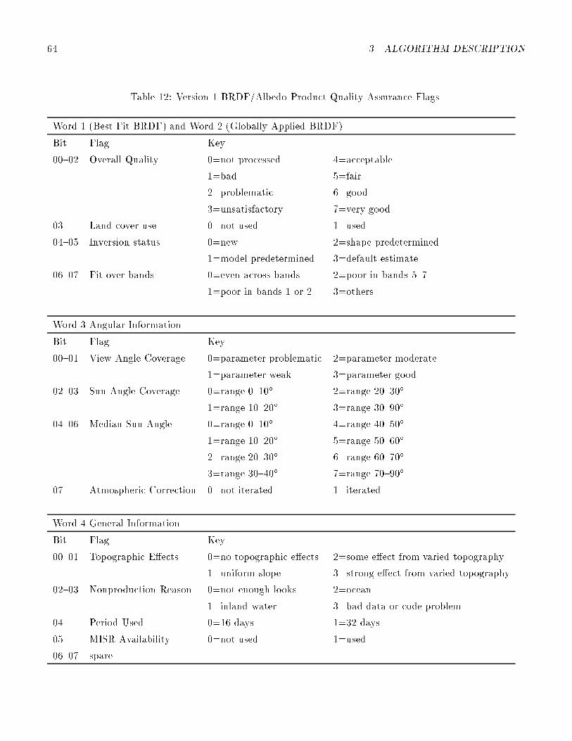
64 3 ALGORITHM DESCRIPTION
Table 12: Version 1 BRDF/Albedo Product Quality Assurance Flags.
Word 1 (Best Fit BRDF) and Word 2 (Globally Applied BRDF)
Bit Flag Key
00{02 Overall Quality 0=not processed 4=acceptable
1=bad 5=fair
2=problematic 6=good
3=unsatisfactory 7=very good
03 Land cover use 0=not used 1=used
04{05 Inversion status 0=new 2=shape predetermined
1=model predetermined 3=default estimate
06{07 Fit over bands 0=even across bands 2=poor in bands 5{7
1=poor in bands 1 or 2 3=others
Word 3 Angular Information
Bit Flag Key
00{01 View Angle Coverage 0=parameter problematic 2=parameter moderate
1=parameter weak 3=parameter good
02{03 Sun Angle Coverage 0=range 0{10� 2=range 20{30�
1=range 10{20� 3=range 30{90�
04{06 Median Sun Angle 0=range 0{10� 4=range 40{50�
1=range 10{20� 5=range 50{60�
2=range 20{30� 6=range 60{70�
3=range 30{40� 7=range 70{90�
07 Atmospheric Correction 0=not iterated 1=iterated
Word 4 General Information
Bit Flag Key
00{01 Topographic E�ects 0=no topographic e�ects 2=some e�ect from varied topography
1=uniform slope 3=strong e�ect from varied topography
02{03 Nonproduction Reason 0=not enough looks 2=ocean
1=inland water 3=bad data or code problem
04 Period Used 0=16 days 1=32 days
05 MISR Availability 0=not used 1=used
06{07 spare
65
3.3.7 Data Dependencies
The input data include:
Required data
� Gridded MODIS surface re ectance data (product MOD09) in the seven MODIS land bands (1{7), in-
cluding information on atmospheric state passed to the BRDF/Albedo algorithm as an internal product
� Gridded MISR surface re ectance and atmospheric parameters (MISR Level 2 Aerosol/Surface Product)
� Level 2G Footprint Pointers
� Angular InformationSupporting Data
� The MODIS Land Cover Product (MOD12)
� The BRDF/Albedo product from the prior time period
� An ancillary generic BRDF/Albedo database
� Topographic information on within-pixel slope facet angles and orientations from a 100-m resolution DEM
for topographic correction (postlaunch)
� Atmospheric state
3.3.8 Output Products
Table 1 provides a complete description of the BRDF/Albedo product output . The principal features are:
� Best-�tting BRDF model identi�er, with parameter values, RMS error, black-sky albedo function coe�-
cients and white-sky albedo for the model
� Parameters and RMS error for the modi�ed Walthall model
� A comprehensive set of ags describing overall quality, band-wise quality, sun and view angle coverage,
and consistency for the best- �tting model.
4 CONSTRAINTS, LIMITATIONS, ASSUMPTIONS
Constraints, limitations and assumptions are largely discussed ad seriatim in the body of this document. A
brief itemization is provided below.
4.0.9 ASSUMPTIONS AND CONSTRAINTS
� MISR/MODIS data are georegistered with su�cient accuracy that BRDF/Albedo calculations are not
signi�cantly a�ected by misregistration
. � The resampling inherent in georegistration of MISR radiances does not signi�cantly a�ect BRDF/Albedo
retrievals.
66 4 CONSTRAINTS, LIMITATIONS, ASSUMPTIONS
� The derivation of atmospheric parameters fromMISR and MODIS is su�ciently accurate that BRDF/Albedo
calculations are not signi�cantly a�ected by their errors.
� The physical parameters controlling BRDF/Albedo remain constant during the production cycle, althoughwe plan to screen for obvious changes.
� Topographic e�ects on BRDF can be described within the semiempirical model �tted to the pixel (at
launch) or separated from surface cover (postlaunch)
� The Ambrals semiempirical BRDF model kernel are su�ciently complete to describe well the range of
BRDFs and albedos encountered on the earth's land surface.
4.0.10 LIMITATIONS
The BRDF/Albedo product will be made every 16 days for every land pixel. If the set of surface re ectance
measurements within that period is insu�cient to provide new BRDF and albedo values, a value from an
earlier period or a value based on the ancillary generic data set will be output.
Acknowledgments
We would like to thank Baojin Zhang for work on model inversion accuracy under varying angular sampling,
Jordan Borak for investigating spectral-to-broadband albedo conversion, Matt Disney and Encarna Vives
Ruiz de Lope for excellent work applying the Ambrals model to data at UCL, Zoltan Hesley for work done
at the University of Wales, Robert P. d'Entremont at Atmospheric and Environmental Research for inves-
tigations into the e�ects of cloud cover, and Jim Tallent for taking the beta-version of the Ambrals code to
version 1. This work was supported by NASA under NAS5-31369; in the UK, work was supported partially
by NERC under the TIGER-SVATS programme, and by the European Union under the 3rd Famework
Human Capital and Mobility Programme.

67
5 LITERATURE CITED
Allen, S. J., J. H. C. Gash, M. V. K. Sivakumar, and J. S. Wallace, 1994, Measurements of albedo variationover natural vegetation in the Sahel.: Int. J. Climatology, v. 14, p. 625-636.
Allison, D.A., and J-P. Muller, 1992, An automated system for sub-pixel correction and geocoding ofmultispectral and multi-look aerial imagery, Proc. 17th Cong. Int. Soc. Photogramm. Remote Sens.,Washington DC, August 2-14 1992, 29(B2), pp. 275-285.
Allison, D.A., M. J. Barnsley, P. Lewis, N. Dyble, and J-P. Muller, 1994, Precise geometric registrationof ASAS airborne data for land surface BRDF studies, Proc. Int. Geosci. Remote Sens. Symp.,Pasadena, California, USA, August 8-12 1994, pp. 1655-1657.
Allison, D., M. J. Zemerly and J.-P. Muller, 1991, Automatic seed-point generation for stereo matchingand multi-image registration, Proc. Int. Geosci. Remote Sens. Symp., Espoo, Finland, 3-6 June 1991,pp. 2417-2421.
Arino, O., G. Dedieu and P. Y. Deschamps, 1991, Accuracy of satellite land surface re ectance determina-tion, J. Appl. Met. 30:960-972.
Arino, O., G. Dedieu and P. Y. Deschamps, 1992, Determination of land surface spectral re ectances usingMETEOSAT and NOAA/AVHRR shortwave channel data, Int. J. Remote Sens. 13:2263-2287.
Babey, S. K. and R. J. So�er, 1992, Radiometric calibration of the Compact Airborne SpectrographicImager, Can. J. Remote Sens. 18:233-242.
Barkstrom, B. R., and G. L. Smith, 1986, The Earth radiation budget experiment: Science and implemen-tation, Rev. Geophys. 24: 379-390.
Barnsley, M. J., P. Lewis, J.-P. Muller, and M. Sutherland, 1996, Deriving Improved Estimates of LandSurface Albedo through inversion of BRDF models using NASA-ASAS images of HAPEX- SAHELSouthern Supersite.: J. Hydrology (submitted 4/95, accepted 12/95).
Barnsley, M. J. and S. A. W. Kay, 1990, The relationship between sensor geometry, vegetation-canopygeometry and image variance, Int. J. Remote Sens. 11:1075-1084.
Barnsley, M. J., and J.-P. Muller, 1991, Measurement, simulation and analysis of bidirectional re ectanceproperties of earth surface material, Proc. Int. Conf. Spectral Signatures in Remote Sens., Courchevel,France, January 14-18 1991, pp. 375-382.
Barnsley, M. J., A. H. Strahler, K. P. Morris, and J.-P. Muller, 1994, Sampling the surface bidirectionalre ectance distribution function (BRDF): Evaluation of current and future satellite sensors, RemoteSens. Rev. 8:271-311.
Bicheron, P., M. Leroy, and O. Hautecoeur, 1996, Analysis of airborne POLDER data on boreal forestcovers.: IGARSS'96, p. 1901-1903.
Boissard, P., Akkal, N., Lewis, P., 1996, 3D Plant Modelling in Agronomy. Association of Applied Biolo-gists: Modelling in Applied Biology: Spatial Aspects, 24/27 June 1996, Brunel, U.K.
Borel, C. C., S. A. W. Gerstl and B. Powers, 1991, The radiosity method in optical remote sensing ofstructured 3- D surfaces, Remote Sens. Environ. 36:13-44.
68 5 LITERATURE CITED
Breon, F.-M., V. Vanderbilt, M. Leroy, P. Bicheron, C. L. Walthall, and J. E. Kalshoven, 1996, Evidenceof hot spot directional signature from airborne PODLER measurements: IEEE Trans. Geosci. Rem.Sens., v. in press.
Brest, C. L., and S. N. Goward, 1987, Deriving Surface Albedo Measurements from Narrow-band Satellitedata: Int. J. Remote Sensing, v. 8, p. 351-367.
Brown de Coulstoun, E. C., C. L. Walthall, A. T. Cialella, E. R. Vermote, R. N. Halthore, and J. R.Irons, 1996, Variability of BRDF with land cover type for the West Central HAPEX-Sahel Super Site.:IGARSS'96, p. 1904-1907.
Burgess, D., P. Lewis, and J.-P. Muller, 1995, On topographic e�ects in AVHRR NDVI data: RemoteSensing Environment, v. 54, p. 223- 232.
Choudhury, B. J. and A. T. C. Chang, 1981, On the angular variation of solar re ectance of snow, J.Geophys. Res. 86:465-472.
Coakley, J .A., and F. P. Bretherton, 1982, Cloud cover from high resolution scanner data: Detection andallowing for partially �lled �elds of view, J. Geophys. Res. 87:4917- 4932.
Dedieu, G.,1992, Surface radiation budget in the shortwaves using the METEOSAT ISCCP B2 data-set, Proc. 9th METEOSAT Scienti�c Users' Meeting, Locarno, Switzerland, September 14-18 1992,EUMETSAT, Darmstadt, pp. 69-76.
Deering, D. F., 1989, Field measurements of bidirectional re ectance, in Theory and Applications of OpticalRemote Sensing, G. Asrar, ed., John Wiley & Sons, New York, pp. 14-65.
Dickinson, R. E., 1983, Land surface processes and climate- surface albedos and energy, Adv. Geophys.25:305-353.
Diner, D., J. V. Martonchik, C. Borel, S. A. W. Gerstl, H. R. Gordon, R. Myneni, B. Pinty, and M.M. Verstraete, 1996 MISR LEvel 2 Surface Retrieval Algorithm Theoretical Basis, NASA EOS-MISRDocument, JPL D-22401, Rev. B, 78 pp.
Diner, J. D., C. J. Bruegge, J. V. Martonchik, T. P. Ackerman, R. Davies, S. A. W. Gerstl, K. P. Klaasen,G. W. Lilienthal, D. I. Nakamoto, R. J. Pagano, and T. H. Reilly, 1989, MISR: A Multiangle Imag-ing Spectroradiometer for Geophysical and Climatological Research for EOS, IEEE Trans. Geocsci.Remote Sens. 27:200-210.
Disney, M., J.-P. Muller, P. Lewis, and M. J. Barnsley, 1997, Production and validation of BRDF/albedomaps over HAPEX- SAHEL.: Int. Coll. on Spectral signatures of objects in Remote Sensing.
Engelsen, O., B. Pinty, M. M. Verstraete, and J. V. Martonchik, 1996,Parametric bidirectional re ectancefactor models: evaluation, improvements and applications, Report, Joint Research Centre of the Eu-ropean Commission, EU 16426,, 114 pp.
Gerstl, S. A. W. and A. A. Zardecki, 1985a, Discrete- ordinates �nite-element method for atmosphericradiative transfer and remote sensing, Appl. Optics 24:81-93.
Gerstl, S. A. W. and A. A. Zardecki, 1985b, Coupled atmosphere/canopy model for remote sensing of plantre ectance features, Appl. Optics 24:94-103.
Goel, N. S., 1987, Models of vegetation canopy re ectance and their use in estimation of biophysicalparameters from re ectance data, Remote Sens. Rev. 3:1-212.
69
Goel, N. S., 1989, Inversion of canopy re ectance models for estimation of biophysical parameters fromre ectance data, in Theory and Applications of Optical Remote Sensing, G. Asrar, ed., John Wiley &Sons, New York, pp. 205-251.
Goel, N. S. and I. Rozehnal, 1992, An architecturally realistic model for radiation regime in vegetationcanopies, Proc. Int. Geosci. and Remote Sens. Symp., Houston TX, May 26-29 1992, 1:48-50.
Gustafson, G. B., R. G. Isaacs, R. P. d'Entremont, J. M. Sparrow, T. M. Hamill, C. Grassotti, D. W.Johnson, C. P. Sarkasian, D. C. Peduzzi, B. T. Pearson, V. D. Jakabhazy, J. S. Bel�ore, A. S. Lisa,1994, Support of Environmental Requirements for Cloud Analysis and Archive (SERCAA): AlgorithmDescriptions, Technical Report PL-TR-94-2114, Phillips Lab, Hanscom AFB MA 01731, 100 pp.
Gutman, G., 1992, Anisotropy of visible and near-IR re ectances over land as observed from NOAAAVHRR, Proc. Int. Radiation Symposium, Tallinn, Estonia, pp. 436-439.
Gutman, G., 1994, Normalization of multi-annual global AVHRR re ectance data over land surfaces tocommon sun-target- sensor geometry, Adv. Space Res. 14:121-124.
Henyey, L. G. and T. L. Greenstein, 1941, Di�use radiation in the galaxy, Astrophys. J. 93:70-83.
Holben, B. N., and C. O. Justice, 1980, The topographic e�ect on spectral response from nadir-pointingsensors, Photogramm. Engr Remote Sens. 46(9):1191-1200.
Hu, B., W. Wanner, X. Li, and A. H. Strahler, The sensitivity of atmospheric correction of re ectances tothe surface BRDF, 1996, Proc. 1st Int. Workshop Multiang. Remote Sens., Beijing, China, in press.
Hu, B., W. Wanner, X. Li, and A. Strahler, Validation of kernel-driven semiempirical BRDF models forapplication to MODIS-MISR data, 1996, Proc. Int. Geosci. Rem. Sens. Symp. 96, Lincoln, Nebraska,1669{1671.
Iaquinta, J. and B. Pinty, 1994, Adaptation of a bidirectional re ectance model including the hot-spot toan optically thin canopy, Proc. Sixth Int. Symp. on Physical Measurements and Signatures in RemoteSens., Val d'Isere, France, January 17-21 1994, pp. 683-690
Irons, J. R., K. J. Ranson, D. L. Williams, R. R. Irish and F. G. Huegel, 1991, An o�-nadir pointing imagingspectroradiometer for terrestrial ecosystem studies, IEEE Trans. Geosci. Remote Sens. 29:66-74.
Jupp, D. L. B. and A. H. Strahler, 1991, A hotspot model for leaf canopies, Remote Sens. Environ.38:193-210. Kimes, D. S., 1983, Dynamics of directional re ectance factor distribution for vegetationcanopies, Appl. Optics 22:1364-1372.
Kimes, D. S., W. W. Newcomb, C. J. Tucker, I. S. Zonneveld, W. van Wijngaarden, J. de Leeuw, and G. F.Epema, 1985, Directional re ectance factor distributions for cover types of Northern Africa, RemoteSens. Environ. 18:1-19.
Kimes, D. S., W. W. Newcomb, R. F. Nelson, and J. B. Schutt, 1986, Directional re ectance distributionsof a hardwood and a pine forest canopy, IEEE Trans. Geosci. Remote Sens. GE-24:281-293.
Kimes, D. S., A. G. Kerber and P, J, Sellers, 1993, Spatial averaging errors in creating hemisphericalre ectance (albedo) maps from directional re ectance data, Remote Sens. Environ. 45:85-94.
Kriebel, K. T., 1978, Measured spectral bidirectional re ection properties of four vegetated surfaces, Int.J. Remote Sens. 17:253-259.
70 5 LITERATURE CITED
Lee, T. Y. and Y. J. Kaufman, 1986, Non-Lambertian e�ects on remote sensing of surface re ectance andvegetation index, IEEE Trans. Geosci. Remote Sens. GE-24:699-708.
Leroy, M. and J.-L. Roujean, 1994, Sun and view angle corrections on re ectances derived from NOAA/AVHRRdata, IEEE Trans. Geocsci. Remote Sens. 32:684-697.
Lewis, P., and J.-P. Muller, 1990, Botanical Plant Modelling for Remote Sensing Simulation Studies:International Geoscience and Remote Sensing, p. 1739-1742.
Lewis, P., and E. Vives Ruiz de Lope, 1996, An Application of kernel-driven BRDF Models and AVHRRdata to monitoring Land Surface Dynamics in the Sahel, First Internat. Workshop MultiangularRemote sens., Bejing, China, Sept 1995.
Lewis, P., 1995, On the Implementation of Linear Kernel-Driven BRDF Models. Proc. RSS 95, "RemoteSensing in Action", Southampton, UK, 11-14 Sept, 333-340.
Lewis, P. and M. J. Barnsley, 1994, In uence of the sky radiance distribution on various formulations of theearth surface albedo, Proc. Sixth Int. Symp. on Physical Measurements and Signatures in RemoteSens., Val d'Isere, France, January 17-21 1994, pp. 707-715.
Lewis, P., M. J. Barnsley, M. Sutherland and J.-P. Muller, 1995, Estimating land surface albedo in theHAPEX-Sahel experiment: Model-based inversions using ASAS data, Proc. Int. Geosci. RemoteSens. Symp., Florence, Italy, July 10- 14, 2221{2223.
Lewis, P., and J.-P. Muller, 1992, The Advanced Radiometric Ray-Tracer: ARARAT for plant canopyre ectance simulation, Proc. 29th Cong. Int. Soc. Photogramm. Remote. Sens., Washington DC,pp. 26-34.
Lewis, P., J.-P. Muller, and K. Morris, 1991, Quality assessment of a botanical plant modelling system forremote sensing simulation studies, Proc. Int. Geosci. Remote Sens. Symp., Espoo, Finland, June 3-61991, pp. 1917-1920
Li, X. and A. H. Strahler, 1986, Geometric-optical bidirectional re ectance modeling of a conifer forestcanopy, IEEE Trans. Geosci. Remote Sens. GE-24:906-919.
Li, X. and A. H. Strahler, 1992, Geometric-optical bidirectional re ectance modeling of the discrete-crownvegetation canopy: E�ect of crown shape and mutual shadowing: IEEE Trans. Geosci. Remote Sens.30:276-292.
Li, X., A. H. Strahler, and C. E. Woodcock, 1995, A hybrid geometric optical-radiative transfer approachfor modeling albedo and directional re ectance of the discrete crown vegetation canopy, IEEE Trans.Geosci. Remote Sens. 33:466- 480.
Li, Z., and L. Garand, 1994, Estimation of surface albedo from space: A parameterization for globalapplication, J. Geophys. Res. 99:8335-8350.
Li, Z. and H. G. Leighton, 1992, Narrowband to broadband conversion with spatially autocorrelated re- ectance measurements, J. Appl. Met. 31:421-432.
Liang, S., P. Lewis, R. Dubayah, W. Qin, and D. Shirey, 1996, Topographic e�ects on surface BidirectionalRe ectance scaling.: Int. Workshop on "Multi-angular Remote Sensing: Measurements, Models andApplications", Beijing, Sept 13-18. 17pp.
71
Liang, S. and A. H. Strahler, 1993a, Calculation of the angular radiance distribution for a coupled systemof atmosphere and canopy media using an improved Gauss-Seidel algorithm, IEEE Trans. Geosci.Remote Sens. 31:491-502.
Liang, S. and A. H. Strahler, 1993, An analytic BRDF model of canopy radiative transfer and its inversion,IEEE Trans. Geosci. Remote Sens. 31:1081-1092.
Liang, S., and A. H. Strahler, 1994a, A four-stream solution for atmospheric radiance transfer over anon-Lambertian surface, Appl. Optics 33:5745-5753.
Liang, S. and A. H. Strahler, 1994b, Retrieval of surface BRDF from multiangle remotely sensed data,Remote Sens. Environ. 50:18-30.
Martonchik, J. V., 1997, Determination of aerosol optical depth and land surface directional re ectancesusing multi-angle imagery, J. Geophys. Res., in press.
Meyer, D., 1994, The Estimation of Clear Sky Albedo over a Tallgrass Prairie using the Advanced VeryHigh Resolution Radiometer. Ph.D Dissertation, U. of Michigan, Ann Arbor, MI, 145 pp.
Minnaert, M., 1941, The reciprocity principle in lunar photometry, Astrophys. J. 93:403-410.
Muller, J.-P., and M. Disney, 1997, The impact of spatial scale on BRDF/albedo retrieval over HAPEX-SAHEL using ASAS data.: Rem. Sens. Env., v. in preparation.
Muller, J.-P., M. Disney, and P. Lewis, 1997a, Monte Carlo ray- tracing of millet plants in HAPEX-SAHEL using stereo photogrammetry for assessing BRDF/albedo algorithms.: Rem. Sens. Env. (inpreparation).
Muller, J.-P., M. Disney, P. Lewis, and M. J. Barnsley, 1997b, Spectral albedo maps of the HAPEX-SAHELarea using LANDSAT- TM and multi- ightline ASAS data.: Rem. Sens. Env., in preparation.
Muller, J.-P., and P. Eales, 1990, Global topography accuracy requirements for EOS, Proc. Int. Geosci.Remote Sens. Symp., Washington DC, May 21-24 1990, pp. 1411-1414.
Muller, J.-P., and M. Dalton, 1988, Application of ray- tracing to satellite image understanding, Proc. Int.Geosci. Remote Sens. Symp., Edinburgh, September 13-16 1988, pp. 1187-1190.
Myneni, R. B., G. Asrar and S. A. W. Gerstl, 1990, Radiative transfer in three dimensional leaf canopies,Transport Theory and Stat. Physics 19:205-250.
Myneni, R. B., G. Asrar, and F. G. Hall, 1993, A three-dimensional radiative transfer method for opticalremote sensing of vegetated land surfaces, Remote Sens. Env., 41:105{121.
Nicodemus, F. E., J. C. Richmond, J. J. Hsia, I. W. Ginsberg and T. Limperis, 1977, Geometrical Consid-erations and Nomenclature for Re ectance, Nat. Bur. Stand. Rept. NBS MN-160, 52 pp.
Nilson, T. and A. Kuusk, 1989, A re ectance model for the homogeneous plant canopy and its inversion,Remote Sens. Environ. 27:157-167.
Neu, T. J., R. G. Isaacs, G. B. Gustafson, and J. W. Snow, 1994, Improved cloud analysis for CDFSIIthrough the SERCAA research and development program, Seventh Conf. Satellite Meteorol. Oceanog.,Monterey, CA, June 6-10 1994, pp. 239- 242.
72 5 LITERATURE CITED
Newton, A., Muller, J.-P., & Pearson, J. C. (1991). SPOT-DEM shading and its application to automatedcorrection of topographic and atmospheric e�ects, Proc. Int. Geosci. Remote Sens. Symp., Espoo,Finland, June 3-6 1991, pp. 655- 659.
Otto, G. P., and T. K. W. Chau, Region-Growing Algorithm For Matching Of Terrain Images, Image AndVision Computing, 7, 83 - 94, 1989.
Pinker, R. T. and J. A. Ewing, 1986, E�ect of surface properties on the narrow to broadband spectralrelationship in satellite observations, Remote Sens. Environ. 20:267-282.
Pinty, B., M. M. Verstraete, and R. E. Dickinson, 1989, A physical model for predicting bidirectionalre ectance over bare soil, Remote Sens. Environ., 27:273-288.
Pinty, B., M. M. Verstraete and R. E. Dickinson, 1990, A physical model of the bidirectional re ectance ofvegetation canopies, 2. Inversion and validation, J. Geophys. Res. 95:11,767-11,775.
Prince, S. D., Y. H. Kerr, J.-P. Goutorbe, T. Lebel, A. Tinga, P. Bessemoulin, J. Brouwer, A. J. Dolman,E. T. Engman, J. H. C. Gash, M. Hoep�ner, P. Kabat, B. Monteny, F. Said, P. Sellers, and J.Wallace, 1995, Geographical, biological and remote sensing aspects of the Hydrologic AtmosphericPilot Experiment in the Sahel (HAPEX-SAHEL): Rem. Sens. Env., v. 51, p. 215-234.
Proy, C., D. Tanr and P. Y. Deschamps, 1989, Evaluation of topographic e�ects in remotely-sensed data,Remote Sens. Environ. 30:21-32.
Rahman, H., M. M. Verstraete and B. Pinty, 1993a, Coupled surface-atmosphere re ectance (CSAR) model,1. Model description and inversion on synthetic data, J. Geophys. Res. 98:20,779-20,789.
Rahman, H., B. Pinty and M. M. Verstraete, 1993b, Coupled surface-atmosphere re ectance (CSAR) model,2. Semiempirical surface model usable with NOAA Advanced Very High Resolution Radiometer data,J. Geophys. Res. 98:20,791-20,801.
Ranson, K. J., L. L. Biehl and M. E. Bauer, 1985, Variation in spectral response of soybeans with respectto illumination, view and canopy geometry, Int. J. Remote Sens. 6:1827-1842.
Ranson, K. J., J. R. Irons, and C. S. T. Daughtry, 1991, Surface albedo from bidirectional re ectance,Remote. Sens. Environ. 35:201-211.
Ross, J. K., 1981, The Radiation Regime and Architecture of Plant Stands, Dr W. Junk, The Hague.Rossow, W. B., and L. C. Garder, 1993, Cloud detection using satellite measurements of infrared andvisible radiances for ISCCP, J. Climate 6:2341-2369.
Roujean, J. L., D. Tanre, F. M. Breon, and J. L. Deuze, 1996, Retrieval of land surface parameters for GCMfrom POLDER bidirectional measurements during HAPEX-Sahel.: J. Geophys. Res., v. in press.
Roujean, J. L., Latoy, M., and Deschamps, P. Y., 1992, A bidirectional re ectance model of the earthssurface for the correction of remote sensing data, J. Geophys. Res. 97:20455-20468.
Roy, D. P., 1996, The MODIS Land (MODLAND) Quality Assurance Plan, available [email protected].
Sancer, M. L., 1969, Shadow-corrected electromagnetic scattering from a randomly rough surface, IEEETrans. Ant. Prop. AP-17:577-585.

73
Schaaf, C. B. and A. H. Strahler, 1993, Solar zenith angle e�ects of forest canopy albedos calculated witha geometric-optical bidirectional re ectance model, IEEE Trans. Geosci. Remote Sens. 31:921-927.
So�er, R. J. and J. R. Miller, 1995, Bidirectional re ectance factors (BRF) of an open tree canopy bylaboratory simulation, Proc. 17th Can. Remote Sens. Symp., Saskatoon, Canada, June 1995.
So�er, R., Miller, J., Wanner, W., and Strahler, A.H., 1995, Winter boreal forest canopy BRF results:Comparisons between airborne data, laboratory simulations and geometrical-optical model data, Proc.1995 Internat. Geosci. Remote Sens. Symp., Florence, Italy, July 10-14, 1995, vol 1., pp. 800-802.
Starks, P. J, J. M. Norman, B. L. Blad, E. A.Walter-Shea and C. L. Walthall, 1991, Estimation of shortwavehemispherical re ectance (albedo) from bidirectionally re ected radiance data, Remote Sens. Environ.38:123-134.
Stowe, L. L., E. P. McClain, R. Carey, P. Pellegrino, G. G. Gutman, P. Davis, C. Long and S. Hart, 1991,Global distribution of cloud cover derived from NOAA/AVHRR operational satellite data, Adv. SpaceRes. 11:51-54.
Strahler, A. H., 1994, Vegetation canopy re ectance modelingrecent developments and remote sensingperspectives, Proc. Sixth Int. Symp. Physical Measurements Spectral Signatures, Val d'Isere, France,January 17-21 1994, pp. 593-600.
Strahler, A. H. and S. Liang, 1994, Comparisons of radiative transfer models of vegetation canopies withlaboratory measurements, Proc. Int. Geosci. Remote Sens. Symp., Pasadena, California, USA,August 8-12 1994, 4:2345-2347.
Strahler, A. H., W. Wanner, Q. Zhu, and X. Jin, 1995, Bidirectional re ectance modeling of data forvegetation obtained in the Changchun Solar Simulation Laboratory, Proc. Int. Geosci. Remote Sens.Symp., Florence, Italy, July 10-14 1995, 1965{1967.
Taylor, V. R. and L. L. Stowe, 1984, Re ectance characteristics of uniform Earth and cloud surfacesderived from NIMBUS-7 ERB, J. Geophys. Res. D89:4987-4996. Teillet, P. M., and K. Staenz, 1993,Atmospheric e�ects due to topography on MODIS vegetation index data simulated from AVIRISimagery over mountainous terrain, Can. J. Remote Sens. 18:283-292.
van Leeuwen, W. J. D., A. R. Huete, S. Jia, and C. L. Walthall, 1996, Comparison of Vegetation Indexcompositing scenarios: BRDF vs. Maximum VI approaches.: IGARSS'96, p. 1423-1425.
Vermote, E., D. Tanr, J. L. Deuze, M. Herman, and J. J. Morcrette, 1994, Second Simulation of the SatelliteSignal in the Solar Spectrum (6S), User Guide, available from E. Vermote, GSFC.
Vermote, E. F., N. El Saleous, C. O. Justice, Y. J. Kaufman, J. L. Privette, L. Remer, J. C. Roger, and D.Tanre, 1997, Atmospheric correction of visible to middle infrared EOS-MODIS data over land surface:background, operational algorithm and validation, J. Geophys. Res., in press.
Verstraete, M. M., B. Pinty and R. E. Dickinson, 1990, A physical model of the bidirectional re ectance ofvegetation canopies, 1. Theory, J. Geophys. Res. 95-755- 765.
Walthall, C. L., J. M. Norman, J. M. Welles, G. Campbell and B. L. Blad, 1985, Simple equation toapproximate the bidirectional re ectance from vegetation canopies and bare soil surfaces, Appl. Optics24:383-387.
74 5 LITERATURE CITED
Wanner, W., X. Li, and A. H. Strahler, 1995, On the derivation of kernels for kernel-driven models ofbidirectional re ectance, J. Geophys. Res., 100: 21077{21090.
Wanner, W., A. Strahler, J.-P. Muller, M. Barnsley, P. Lewis, X. Li and C. Barker Schaaf, 1995, Globalmapping of bidirectional re ectance and albedo for the EOS MODIS project: The algorithm and theproduct, Proc. Int. Geosci. Remote Sens. Symp., Florence, Italy, July 10-14 1995, 525{529.
Wanner, W., A. H. Strahler, B. Hu, P. Lewis, X. Li, J.-P. Muller, and M. J. Barnsley, 1996, Global BRDFand albedo from the EOS MODIS and MISR sensors, Proc. 1st Int. Workshop Multiang. RemoteSens., Beijing, China, in press.
Wanner, W., A. H. Strahler, B. Zhang, and P. Lewis, Kilometer-scale global albedo from MODIS, 1996.Proc. Int. Geosci. Rem. Sens. Symp. 96, Lincoln, Nebraska, 1405{1407.
Wanner, W., P. Lewis, and J.-L. Roujean, The in uence of directional sampling on bidirectional re ectanceand albedo retrieval using kernel-driven models, 1996, Proc. Int. Geosci. Rem. Sens. Symp. 96, Lincoln,Nebraska, 1408{1410.
Wanner, W., A. H. Strahler, B. Hu, X. Li, C. L. Barker Schaaf, P. Lewis, J.-P. Muller, and M. J. Barnsley,1997, Global retrieval of bidirectional re ectance and albedo over land from EOS MODIS and MISRdata: theory and algorithm, J. Geophys. Res., accepted.
Whittaker, E., and G. Robinson, 1960, The Calculus of Observations, Blachie and Son, Glasgow, 397 pp.
Wu, A., Z. Li and J. Cihlar, 1995, E�ects of land cover type and greenness on advanced very high resolutionradiometer bidirectional re ectances: analysis and removal, J. Geophys. Res., 100: 9179{9192.
Wylie, D. P., W. P. Menzel, H. M. Woolf and K. I. Strabala, 1994, Four years of global cirrus cloud statisticsusing HIRS, J. Climate, vol 7, pp. 1972-1986.
Wylie, D. P., and W. P. Menzel, Two years of cloud cover statistics using VAS, J. Climate, 2, 380{392,1989.

75
6 RESPONSE TO ATBD REVIEWS
6.1 1994 REVIEW: Comments and Response
6.1.1 Comments from the Reviewers (June, 1994)
A numerical assessment was made in six categories for each of the individual ATBDs:
1. Degree to which product meets EOS priorities
2. Soundness (feasibility/practicality) of approach
3. Appropriateness of algorithm input
(a) Intermediate Products
(b) Dependence on other AM products
(c) Ancillary data (nonplatform data)
4. Completeness of sensitivity and error budget
5. Soundness of validation strategy
6. Release of useful products at launch
7. Other comments
Each category was given a numerical grade as follows:
Grade 9 | High or strongly agree
Grade 5 | Neutral
Grade 1 | Low
Grade 0 | Insu�cient Information
The BRDF/Albedo product was rated as follows:
1. (Grade 9) Two products wil result from this algorithm (i) the BRDF and (ii) surface albedo. The
latter is obtained by angular and spectral integration of the BRDF. Both products are relevant to the MTPE
programs.
2. (Grade 6) The proposed approach could be enormously complex to implement. It has never been
tried over as large a region as even a single satellite pixel, and therefore is high risk for producing reliable
global products by launch.
3. (Grade 8) (a) With dependence on the AM products as an additional complication, the developers
propose to invert a coupled atmosphere-surface model, obtaining simultaneously the atmospheric and canopy
properties. This renders the problem even more complex and spectral region dependent. Land cover maps
will also be needed. The land cover classes needed to do this will likely be more complex and �ner spatial
resolution than those required by the ecosystem process models. Who will produce these maps? The problem

76 6 RESPONSE TO ATBD REVIEWS
would be much less complex were the developers to use atmospherically corrected data. The algorithm will
also need cloud-screened data. (b) As to the appropriateness of intermediate products, it is not clear
that there will be any EOS algorithms that utilize the BRDF data directly without further synthesis into
products such as albedo. There is no question however, that BRDF data would be enormously useful for
many computations and investigations. (c) As for the need for ancillary data, topographic data will be
critical to the model inversion problem as well as meteorological data to analyze canopy status to initialize
the BRDF inversions. Other data such as soils maps, global land cover maps etc. would be needed.
4. (Grade 0) No error modeling or sensitivity analysis is presented.
5. (Grade 0) No validation strategy is presented.
6. (Grade 1{5) Given the immaturity of the this algorithm, the probability of BRDF data generated at
1km globally is very unlikely. Even with an algorithm, it is not clear how many orbits will be required to
build up the requisite cloud{free views to develop a reliable BRDF. Thus, the BRDF product will likely be
one where the holes are slowly �lled in.
7. (Comments) It is not obvious how the complete BRDF can be constructed from MISR. Much of the
variability and asymmetry occurs near the principal plane for which even the scan{plane of MODIS will
not come close in certain seasons. It is also not clear given cloud cover probabilities in most vegetated
regions, how long it will take to acquire enough data to build the BRDF. Multiple acquisitions at several
di�erent relative azimuths may be required for some vegetation types. In addition, the implementation of
the approach has not been thought out in detail and will present many practical problems when attempting
to implement it on a global scale. The largest practical problem is that no universal canopy re ectance
model exists that can handle the range of canopies to be encountered on a global scale. To circumvent
this problem, the developers propose several di�erent models, to be selected to address the complexity of
di�erent ecosystems. Thus a logic will need to be worked out, with objective criteria speci�ed, for selecting
which model to use for what pixel. This selection criteria might also need to select di�erent models for
di�erent MODIS bands since models for bands where multiple scattering is not important might not work
for bands for which multiple scattering dominates. This will require a front end to the algorithm to generate
the input parameters to the criteria.
It is not made clear how the MODIS and MISR data will be combined to produce the BRDF since
di�erent bands and spatial resolutions are involved. The developers propose to produce a BRDF for each
1 km. This will potentially present a large processing load, and in fact may be unnecessary where large
portions of an ecosystem might be rather homogeneous over several kilometers. The approach does not rely
on direct observation of BRDF, rather it infers it from inversion of re ectance models to obtain surface
parameters, but very little, if any work has been done using the extracted parameters to construct a BRDF
for the purpose of computing surface albedo.
6.1 1994 REVIEW: Comments and Response 77
6.1.2 Algorithm Changes in Response to the 1994 Review
Here is a summary of the major changes in the algorithm:
G1. Use of semiempirical models.
BRDF is now �tted using a suite of simple, linear, semiempirical models. In e�ect, these models �t the
angular pattern of observed bidirectional re ectance measurements using a mixture of simple, contrasting
BRDF shapes that are derived by simplifying more complex physical BRDF models. That is,
R = fiso + fgeokgeo + fvolkvol (41)
where R is the BRDF as a function of illumination zenith, view zenith, and relative azimuth; kgeo and kvol
are two shape functions that depend only on illumination zenith, view zenith, and relative azimuth; fgeo
and fvol are weights that mix the two BRDF shapes; and fiso is a constant, corresponding to isotropic
(Lambertian) BRDF shape.
The shape function kgeo is derived from BRDF theory for surfaces dominated by geometric-optical shad-
owing e�ects. There are currently three choices for this function, derived from the theory of (1) rectangular
projections on a plane; (2) sparse spheroidal projections on a plane; and (3) dense spheroidal projections
on a plane. The shape function kvol is derived from theory describing the volume scattering of leaves in
a homogeneous layer. Two choices are currently available for this shape function, derived from theory for
(1) thin, and (2) thick, leaf layers. A third volume-scattering shape function, derived from the theory of
volume scattering of snow, is under development. We also �t the Walthall model for BRDF, which is of a
mathematical form similar to that above, but relies on empirical functions rather than BRDF shapes derived
from physical models.
G2. Inversion speed.
The algorithm now runs very quickly. Fitting a single semiempirical model requires only inversion of
a 3 by 3 matrix. This allows us to �t multiple combinations of models and choose the one with the best
�t. Realistic timings of the algorithm in execution now fall easily within instrument and product resource
allocations.
G3. 16-day cycle instead of 9-day.
Following preliminary studies of cloud cover, we now plan to provide the product on a 16-day cycle,
instead of a 9-day cycle. (Sixteen days is the repeat cycle for double MISR coverage { that is, the 16-day
cycle provides at least two possible MISR acquisitions at all latitudes.)
G4. Atmospheric coupling.
The coupling between the atmosphere and surface is accomplished by an iterative loop in which a prior
78 6 RESPONSE TO ATBD REVIEWS
(or Lambertian) BRDF is used to extract surface bidirectional re ectances given their atmospheric state;
a provisional BRDF is �tted; surface bidirectional re ectances are reextracted; and the next BRDF is
calculated. Only one or two loops are needed in nearly all cases to convergence within a few percent. The
atmospheric correction logic is that of the MODIS surface re ectance product (Vermote), similar to that
used in the 6S program. The looping logic follows MISR=D5s approach.
G5. Spatial resolution.
The product is still produced at 1-km resolution (now 1.1 km resolution on the ISSCP Level 3 grid). This
�ne resolution is needed for input to the surface re ectance product, which produces output at (nominal)
250- and 500-m resolutions and requires the BRDF for accurate calculation. However, the linear nature of
the semiempirical models allows easy extrapolation of both BRDF and albedo measures to coarse resolutions.
In this way, the needs of both global climate modelers and regional climate-surface energy balance modelers
for albedo and BRDF data can easily be accommodated.
6.1.3 Speci�c Responses to the Panel's Comments
P1. Complexity.
The panel notes that the approach described in the old ATBD could be enormously complex to implement
and has never been tried over a region of any size. However, the revised algorithm using semiempirical
models is enormously simpler. Computational tests show that it can be applied globally at reasonable levels
of processing power. We have also applied several semiempirical models (although not the full suite yet)
to ASAS imagery on a pixel-by-pixel basis. We will shortly apply the full algorithm to a registered LAC
dataset of New England. Both of these applications are discussed in more detail in the new ATBD.
P2. Atmospheric Correction.
The panel noted that inverting a coupled atmosphere-surface model produces an added complication.
The new algorithm couples surface and atmosphere in a simple loop that requires one or two iterations. (See
G4. above.)
P3. Error modeling and sensitivity analysis.
The panel notes that no error modeling or sensitivity analysis is presented. The new ATBD provides
such analyses.
P4. Validation.
The panel observes that no validation strategy is presented. The new ATBD provides an extensive
discussion of validation.

6.1 1994 REVIEW: Comments and Response 79
P5. Scan geometry for MODIS and MISR.
The panel expressed the concern that between MODIS and MISR, insu�cient observations may be
acquired along the principal plane, where much variability and asymmetry in the BRDF occurs. The
acquisition of observations along the principal plane is a complex function of orbit, sensor geometry, latitude,
and time of the year. Because MISR acquires data in the along-track direction and MODIS in the across-
track direction, there is normally good coverage of the view hemisphere, with observations from one or the
other instrument near the principal plane. The subject is treated in more detail in our recently published
paper (Barnsley et al., 1994) and in the new ATBD. Note that the use of semiempirical models, in which
the BRDF shapes are physically-based, mitigates this problem. Since the BRDF shape is restricted by the
physics and is not allowed to vary freely, principal plane measurements are less important.
P6. Cloud cover.
The panel pointed out that, given cloud cover, it is not clear how long it will take to acquire enough
observations to �t a BRDF. We are investigating the cloud cover problem, and as a result of studies described
in the new ATBD, we have changed the product cycle from 9-day to 16-day. (See G3. above.)
P7. Model selection.
The prior algorithm relied on a selection process to choose an appropriate physical BRDF model to invert
on a pixel-by-pixel basis. The panel was concerned that this process was not su�ciently well thought- out
or speci�ed. The new algorithm eliminates this selection process.
P8. Data combination.
The panel pointed out that the issue of combining MISR and MODIS data with varying spatial and
spectral resolutions was not well speci�ed in the ATBD. This has been remedied in the new document.
P9. 1-km resolution.
The panel was concerned that the 1-km spatial resolution presented a large processing load, and that for
at least some regions, large portions of an ecosystem might be rather homogeneous over several kilometers.
With the speed of the new algorithm, the processing load is no longer a problem. Although there may
be some large, homogeneous regions with unchanging BRDF, there will certainly be other regions where
�ne-grained land surface variation will require �ne resolution of the BRDF and albedo. Note also that
for accurate results, the surface re ectance algorithm (Vermote) requires BRDF at as �ne a resolution as
practical.
P10. Albedo from BRDF.
The panel comments that little, if any, work has been done on the construction of a BRDF for the purpose
of computing a surface albedo. Actually, there is long history of this for TOA BRDFs in the asymmetry
80 6 RESPONSE TO ATBD REVIEWS
factors of Taylor and Stowe (1984) for ERB and follow-on work (e.g., Baldwin and Coakley, 1991; Green and
Smith, 1991). For surface measurement, a number of recent papers have used BRDF functions in relating
directional measurements to albedo (e.g., Ranson et al., 1991; Starks et al., 1991). So some work of this
nature has been done, and more is likely to be on the way. Combining bidirectional measurements through
the mechanism of a BRDF is really the only way to measure the albedo of a small patch of land surface
directly from space. Other approaches (e.g., Sellers et al., 1994) require even more modeling.
P11. Land cover information.
The panel notes that �ne-grained land cover information is needed for the model-selection procedure
(see 3. above) and that appropriate data might not be available. Land cover information is not used for
model selection operationally in the new algorithm, although it may be used to "prime the pump" at time
zero. Land cover information will be available at launch, probably as the IGBP 1-km Land Cover Database
derived from the global 1-km AVHRR NDVI composite now being processed at EDC (see Land Cover
Product ATBD).
P12. Use by other EOS algorithms.
The panel remarks that it is not clear that there are any EOS algorithms that utilize the BRDF data
directly. However, MODIS surface re ectance uses BRDF directly. This is because the errors induced by
assuming isotropic surface re ectance can be as large as 15 percent for turbid cases (discussed in new version
of ATBD). Calculations by Lee and Kaufman documented this back in 1986. We are presently working with
Eric Vermote to integrate the BRDF and surface re ectance algorithms together into a single processing
chain.
P13. Ancillary data.
The panel remarks that extensive ancillary data (topographic, soils, meteorological) are needed. However,
these were for the model selection procedure that is now eliminated.
6.1.4 Speci�c Responses to the Mail Reviewers' Comments
For the mail reviewers, many speci�c comments are obviated by the changes in the both the algorithm and
document. Thus, the responses below are directed to the more general concerns that they express.
Ross-Nilson-Kuusk
R1. Choice of re ectance models is problematic.
This review commented that other physical models should be explored. However, our product no longer
uses physical models{just semiempirical models. The review also expressed some concern about the vali-
dation of the Liang-Strahler model against radiative transfer calculations. Again, this model is no longer
6.1 1994 REVIEW: Comments and Response 81
used. The model selection issue, commented on in P7. above, was also raised. Use of semiempirical models
obviates the problem.
R2. Atmospheric coupling.
These reviewers suggest that atmospheric coupling is important and needed to be developed in more
detail in the document. This has been done.
R3. Albedo calculation.
The review requested better development of the procedure for calculating albedo from integrating the
BRDF, noting problems with atmospheric e�ects and pixel sizes at large view zenith angles. Both of these
issues are now addressed in the new ATBD.
R4. Multisensor, multichannel data needed.
The review noted that retrieval of physical parameters from inversion of physical models can be prob-
lemmatic and that additional multisensor, multichannel data may be required to provide good accuracy.
However, the algorithm no longer inverts physical models to infer physical parameters.
Borel-Gerstl
B1. Mixed pixels.
These reviewers point out that MODIS-sized pixels will contain mixtures of cover types, and individual
physical models may not �t them well. Further, there were cover types that were not �tted well by any of the
physical models we had selected, such as snow, standing water, etc. In the new algorithm, the semiempirical
models handle mixtures easily and should be able to accommodate these other cover types without di�culty.
B2. Inversion issues.
The reviewers express concerns about numerical inversion procedures (no longer required); the processing
power needed for global calculations (not a problem for the semiempirical models, see G2. above); e�ects of
noise on inversion (new sensitivity studies in ATBD show good results); computational costs of numerical
integration of BRDFs to give albedo measures (now trivial due to �xed kernels with variable weights and a
linear model); and that maps of BRDF parameters from multiangular data have never been produced (now
included in the new ATBD).
B3. Global use of Walthall model.
The reviewers suggest we consider use of a few simpler models, and suggest the Walthall et al. (1985)
model as a candidate. We have, in e�ect, taken their advice by using the semiempirical models.
82 6 RESPONSE TO ATBD REVIEWS
B4. MODIS-MISR data combination issues.
The reviewers note that the issues of merging MISR and MODIS data are not well addressed in the
document. The issues include not only geometry but also the fact that sun angle and atmospheric condition
will vary with each MODIS image. A new section in the revised ATBD handles the data merging issue,
and the atmospheric correction procedure accepts the fact that the atmosphere is di�erent for each MODIS
observation. See also P5. above.
B5. Research issues.
The reviewers list several issues that require more study: (1) the number of observations needed to derive
the BRDF of a pixel (10 is our cuto�, but sensitivity studies have not been done yet); (2) the sensitivity
of the retrieved parameters to errors introduced by noise and errors in atmospheric correction (some noise
studies are complete and in the new ATBD, others are planned); (3) the e�ects of registration errors on
BRDF parameter extraction for heterogeneous surfaces (studies are planned); and (4) the allowable interval
in which can we consider the BRDF of a vegetation cover to be constant (16 days, we hope, with studies
planned for spring/fall AVHRR data to see how quickly BRDF/Albedo changes).
Meyer Review
M1. Land cover dependence.
This reviewer notes that in our prior algorithm, land cover information was used in model selection,
raising issues of updating of land cover information in the face of land cover change on a three-month
time scale, while BRDF/Albedo was observed much more frequently. However, model selection is no longer
necessary, obviating the need for land cover for this purpose.
M2. Sensitivity to atmospheric in uences.
More sensitivity studies detailing the e�ect of atmospheric correction errors on model parameter retrieval
need to be done, according to the reviewer. We agree, and plan such studies.
M3. Sensitivity to geometric and radiometric errors.
Angular, geolocational and spectroradiometric errors need to be investigated systematically in the context
of merging MODIS and MISR data. We agree, and plan such studies.
Verstraete Review
Note that this review is exceedingly lengthy (14.5 pages of 10-point type), and that most of the detailed
comments related to the speci�c text by page and paragraph. Since the text has been entirely rewritten,
these no longer apply. The response here is directed toward the overall evaluation paragraphs that begin
6.1 1994 REVIEW: Comments and Response 83
the review.
V1. Algorithms are not suitable for operational products.
The reviewer is concerned that the proposed algorithms are under development and mostly suitable for
academic research. However, with the new semiempirical model approach, we believe we have now developed
algorithms suitable for operational products. (See G2 above.)
V2. Per-pixel BRDF is unrealistic and of low interest.
The reviewer expresses the concern that the computer resources needed for per-pixel determination are
large and that there is not much scienti�c interest in the results. However, the semiempirical model algorithm
now runs well within the resources available for the MODIS instrument and AM platform. (Timings are
documented in the new ATBD.) As for scienti�c interest, the panel review states, "There is no question...
that BRDF data would be enormously useful for many computations and investigations." Note also that to
deliver surface re ectance accurately from MODIS, BRDF is required.
V3. Albedo needs a clearer de�nition.
The new ATBD clearly speci�es the albedo measures we provide in de�nitions traceable from Nicodemus'
classic NBS monograph.
V4. De�ciencies in science, numerical analysis.
The reviewer o�ers the opinion that various parts of the algorithm su�er from de�ciencies in science
and numerical analysis. However, the semiempirical approach we have now selected for the product is fully
grounded in the science of BRDF modeling as it has developed over the past decade or so. Numerical
inversion is no longer necessary, thus obviating this concern.
V5. Prerequisite datasets.
The reviewer notes that the algorithm was dependent on collateral datasets for model selection that were
not well speci�ed. As noted before, the new algorithm operates independently and these datasets are no
longer required.
V6. Relative contributions of MODIS and MISR to the data pool.
The reviewer expresses the concern that since the product will only be produced when MISR data are
available, the contribution of MODIS to the data pool will be minor. (1) The new algorithm will not be
limited to pixels for which MISR data are available, and will provide a product for every pixel every 16
days. If there are insu�cient observations to update the BRDF and albedo, we will reach back to the prior
product or use a stock BRDF/Albedo based on prior experience and past history with the pixel. Flags will
inform the user in these cases. (2) For accurate BRDF retrieval, both MISR and MODIS data are needed,
84 6 RESPONSE TO ATBD REVIEWS
because the two instruments sample the viewing hemisphere from di�erent directions. The contribution of
MODIS is no less important than that of MISR. See P5. above. The exact mixture of MODIS and MISR
observations for a pixel during a time period will be a function of cloud cover during the period.
V7. More detail is needed on issues of scale, spectral bands, accuracy, coregistration, the e�ect of clouds on
data availability, and computations of albedo in SWIR bands.
We agree that these topics all need more work. Of these issues, we have concentrated on accuracy and
cloud impacts, and our results are provided in the revised document. Future studies are planned to address
all of these areas more fully.
V8. Albedo and BRDF are part of the same product, even though the user communities may be di�erent.
The reviewer observes that the user communities and requirements for albedo may be quite di�erent from
those of BRDF, and that alternative strategies for global albedo products should be considered and discussed.
Albedo is a product that is consumed on a number of scales. Needs can range from coarse resolution (e.g.,
1-degree) values that change in the spring and fall for global climate modeling to �ne- resolution data that
is directly ingestible by regional climate and surface energy balance models operating at �ner time scales.
At coarse resolution, there are a number of approaches, well summarized by Li and Garand (1994), ranging
from table lookup based on land cover to derivation of TOA albedo from such data sources as ERBE sensors
and correction of that TOA albedo to surface albedo through empirical corrections derived from radiative
transfer simulations. Whatever the approach, all satellite applications must overcome problems of clear
scene identi�cation, spectral and angular corrections, and the removal of atmospheric e�ects. MODIS and
MISR, by virtue of their �ne resolution yet global coverage, are more suited to provide �ne resolution albedo
products. At the �ne resolution, we see no viable alternative to extracting albedos through the mechanism
of the BRDF (see P10. above), given the spatial and temporal variability of the earth's surface at the 1-km,
biweekly time scale. Had the reviewer been more speci�c, we might be able to respond more speci�cally.
V9. Physical models are home-grown.
The reviewer notes that the physical BRDF models selected rely largely on the work of authors, and a
more open policy of model selection is desirable. Although the set of physical models in the prior algorithm
focused largely on those developed with MODIS support for the MODIS/MISR application, the semiempiri-
cal models draw more broadly on the work of the BRDF community. Models of Roujean (1992), Ross (1981),
and Walthall et al. (1985) as modi�ed by Nilson and Kuusk (1989) are integrated into the algorithm, and
the forward-scattering kernel of Sancer (1969) as used by Choudhury and Chang (1981) will soon be added.
The suite of semiempirical models we have developed has been requested by, and provided to, a number of
key researchers in the �eld, including Roujean, Meyer, Ross, and J. Miller, who are assessing its application.
It is also being tested by colleagues C. Zhu and Q. Zhu in China.

6.1 1994 REVIEW: Comments and Response 85
6.1.5 Literature Cited
Baldwin, D. G. and J. A. Coakley, Jr., 1991, Consistency of Earth Radiation Budget Experiment bidirectional
models and the observed anisotropy of re ected sunlight, J. Geophys. Res. 96:5195-5207.
Barnsley, M. J., A. H. Strahler, K. P. Morris, and J.-P. Muller, 1994, Sampling the surface bidirectional
re ectance distribution function (BRDF): Evaluation of current and future satellite sensors, Remote Sens.
Rev. 8:271-311.
Choudhury, B. J. and A. T. C. Chang, 1981, On the angular variation of solar re ectance of snow, J.
Geophys. Res. 86:465-472.
Green, R. N. and G. L. Smith, 1991, Shortwave shape factor inversion of Earth Radiation Budget
observations, J. Atmos. Sci. 48:390-402.
Lee, T., and Y. J. Kaufman, 1986, The e�ect of surface nonlambertianity on remote sensing, IEEE Trans.
Geosci. Remote Sens., GE24:699-708.
Li, Z., and L. Garand, 1994, Estimation of surface albedo from space: A parameterization for global
application, J. Geophys. Res. 99:8335-8350.
Nilson, T. and A. Kuusk, 1989, A re ectance model for the homogeneous plant canopy and its inversion,
Remote Sens. Environ., 27:157-167.
Ranson, K. J., J. R. Irons and C. S. T. Daughtry, 1991, Surface albedo from bidirectional re ectance,
Remote Sens. Environ. 35:201-211.
Ross, J. K., 1981, The Radiation Regime and Architecture of Plant Stands, The Hague: Dr W. Junk.
Roujean, J. L., Latoy, M., and Deschamps, P. Y., 1992, A bidirectional re ectance model of the earth's
surface for the correction of remote sensing data, J. Geophys. Res. 97:20455-20468.
Sancer, M. L., 1969, Shadow-corrected electromagnetic scattering from a randomly rough surface, IEEE
Trans. Ant. Prop. AP-17:577-585.
Sellers, P. J., C. J. Tucker, G. J. Collatz, S. O. Los, C. O. Justice, D. A. Dazlich and D. A. Randall,
1994, A global 1-degree by 1-degree NDVI data set for climate studies. Part 2: The generation of global
�elds of terrestrial biophysical parameters from the NDVI, Int. J. Remote Sens., in press.
Starks, P. J., J. M. Norman, B. L. Blad, E. A. Walter-Shea, and C. L. Walthall, 1991, Estimation
of shortwave hemispherical re ectance (albedo) from bidirectionally re ected radiance data, Remote Sens.
Environ. 38-123-134.
Taylor, V. R. and L. L. Stowe, 1984, Re ectance characteristics of uniform Earth and could surfaces
serived from NIMBUS-7 ERB, J. Geophys. Res. 89:4987-4996.
Walthall, C. L., J. M. Norman, J. M. Welles, G. Campbell and B. L. Blad, 1985, Simple equation to
approximate the bidirectional re ectance from vegetation canopies and bare soil surfaces, Appl. Optics
24:383-387.

86 6 RESPONSE TO ATBD REVIEWS
6.2 1996 EOS LAND REVIEW: Comments and Response
6.2.1 Comments from the Reviewers (Sept, 1996)
A numerical assessment was made in four categories of evaluation criteria and near{ and long{term recom-
mendations were prepared for each of the individual land products:
1. Technical/soundness of algorithm/approach
2. Value of data product to the Land science community
3. Soundness of the validation strategy
4. Extent to which the 1994 ATBD Review issues have been addressed
5. Near{term recommendations for improvements to the data product
6. Long{term recommendations for improvements or additions to the data product
In addition, the reviewers were asked to evaluate the balance of AM-1 Land Data Products and decide
whether they met the needs of the Land science community.
1. Extent to which the ATBD addressed the compatibility of this data product with other instruments data
products and the needs of the community
2. Assessment of plans for the comparison or enhancement of similar data products from other instruments.
3. Recommendations to improve the balance of land data products
Each category was given a numerical grade as follows:
Grade 9 | Excellent, strongly agree or high
Grade 5 | Average, neutral, medium
Grade 1 | Poor/needs work, disagree, or low
N/A | Not applicable
6.2 1996 EOS LAND REVIEW: Comments and Response 87
The BRDF/Albedo product was rated as follows:
Product
a. (Grade 5) The basic approach chosen by the team reduces to a sophisticated non{linear regression
analysis | �tting a non{linear function to 6-10 points. They chose this simple approach to make it only
observation{based, robust, rapid and scaleable. There are a few concerns/questions that arise based on the
ATBD documentation provided:
1. The kernels assume that BRDF depends only on the relative azimuth angle between sun and view
directions. This assumes azimuthally isotropic vegetation, an assumption not applicable to row crops
or orchards; a caveat that should be noted in the ATBD.
2. The �t and the values of weights will depend upon the data points, especially if the scene is heteroge-
neous. For example, if one deletes a few of the observations,(e. g., hot spot direction, viewing parallel
to the row direction etc.) the �t may be better. Likewise, addition of some observations may make
the �t worse. In other works, the calculated surface re ectance for a given scene/target may depend
on what data points are chosen, not a desirable situation.
3. RMS error is not the most desirable measure. For example, a calculated re ectance of 0.60 vs. measured
re ectance of 0.55 will contribute 0.0025 to RMS error, same as calculated re ectance of 0.08 and
measured re ectance of 0.03, although in the latter case the �t is extremely poor. The team should
consider using percentage (or fractional) RMS error or another alternative measure. (It is noted that
the team has been investigating the �tting stability as a function of di�erent scenarios of data sampling
with MISR or MODIS, as has been reported at the IGARSS'96 meeting. These results shold be very
helpful in addressing the above concerns and need to be documented in the ATBD).
4. If the derived BRDF is used to estimate biophysical parameters, it is likely that the estimation of
the structural parameters will be inaccurate because of the smoothing e�ect of the �tting procedure.
Consideration might be given to giving more weight to near{nadir observations in biophysical retrievals.
5. Is there a linear relationship between the weights as calculated for say 256 1km by 1km pixels and one
16km by 16km pixel: If not, the whole approach (which combines MODIS and MISR data at di�erent
resolution levels) is awed. Scaleability needs to be studied.
6. A 16 day product was chosen to ensure enough cloud{free re ectance data for �tting. For certain
cases, vegetation will signi�cantly change in such a period. Another big concern (based on some work
with AVHRR) is that there will not be enough good observations to �t a function. This will almost
certainly be true at latitudes north of 45� over land in summer. What will the algorithm do then?
With a rapid seasonal change it may not be feasible to extend the permissible period.

88 6 RESPONSE TO ATBD REVIEWS
7. The surface re ectance calculated used a particular atmospheric scattering mode. Will the calculated
BRDF represent the right boundary condition for another atmospheric scattering model?
8. MISR data are not available for wavelengths used in MODIS bands 5{7. The model selection is done
using MODIS/MISR data in Bands 1{4. Thus it is assumed that BRDF shape in Bands 5-7 follows
the general shape in Bands 1{4. Is this a justi�able assumption?
b. (Grade 5) BRDF and albedo are useful for biophysical and climate modeling, angle correction of land sur-
face re ectances, a lower boundary condition for atmospheric radiative transfer, and surface energy balance
calculations. For example, the landcover product needs equivalent nadir re ectances, and the hydrological
(climate) modeling community needs monthly albedo data at 10 (50) km spacing . Many of the atmospheric
correction models assume a Lambertian earth to get surface re ectance and radiance and knowledge of the
earth BRDF will improve corrections.
However, the quality of the product, especially BRDF, may not be good for certain purposes. See com-
ments under technical/scienti�c soundness.
c. (Grade 5) The validation approach consists of �tting the semi{empirical model to a wide range of �eld{
measured BRDF sets (from literature), aircraft{measured data (ASAS, POLDER, CASI), laboratory data
and simulated data. The team also plans to do large scalestudies.
Since the general model has many parameters, one would expect that the model will �t to the observed
data (PARABOLA or ASAS). What is important is what happens to the �tted parametres if the data poinst
are changed and some of the points have measurement erros. If the �tting approach is not \stable", the
validity of the whole approach is questionable. However, see the comments above regarding the �tting tests
being reported by the team at the recent IGARSS'96 meeting.
d. (Grade 7) Before the 1994 ATBD review, the team were planning to use physical BRDF modeling and the
reviewers raised several concerns about the physical approach, included the operational feasibility, need of
ancillary data, adequacy of the angular data. In response to the comments, the team has completely changed
the approach to the present semiemipirical approach. The physical approach has its attractive features. The
panel urges a longer{term EOS strahtegy that adopts the semi{empirical approach for an at-launch product
but is open to a new initiative for an advanced post-launch product based on physical{modeling research
program.
e. Near{term recommendations.
� Systematically evaluate the �tting process as a function of number of observations and the solar/viewingdirections of the observations. These \observations" could be generated by a canopy re ectance model or
from an instrument (e. g. PARABOLA). This study should be carried out for heterogeneous canopies.
� Determine how sensitive the product is to the choice of a di�erent atmospheric scattering model, such

6.2 1996 EOS LAND REVIEW: Comments and Response 89
as those used by the ASTER or MISR teams. A collaboration with the atmospheric scattering modeler(s)
who may use the product whould be mutually bene�cial.
� Determine the usefulness of the product in biophysical parameter estimation by carrying out the in-
versions for known vegetation canopies.
f. Long{term recommendations.
� Investigate the possibility of developing an approach which has a proper balance between physical and
empirical modeling, which uses vegetation classi�cation to minimize the complexity.
Balance
a. (Grade 5) BRDF and albedo are very useful for biophysical and climate modeling, angle correction of land
surfaces, and surface energy balance calculations. A knowledge of earth BRDF will improve the accuracy
of ASTER based atmospheric correction to get surface properties. BRDF is also the basis for higher level
biophysical products. Consequently, the quality of the BRDF product is especially important.
b. (Grade 5) On the basis of oral comments, it appears that the team will work with team members from
other instruments, especially MISR. It also appears that the team will use simulated data from MISR and
vice-versa to improve on the product and enhance the data{formate compatibility and explore the comple-
mentarity of MODIS in a synergistic way to improve the accuracy of various surface re ectance products.
c. (Recommendations for change) See comments above.
6.2.2 Speci�c Responses to the Land Review Panel's Comments (Section 5.2.6a of the EOS-
AM-1 Land Data Product Review Report)
Prepared by Alan Strahler, Wolfgang Wanner and Crystal Barker Schaaf
We would like to thank the SWAMP Review Panel for a very thorough and constructive review. The
members of the panel not only brought a great deal of their own understanding and experience to the
review, but also clearly spent a lot of time in a careful examination of our speci�c algorithm. We very much
appreciate their e�orts.
The purpose of this document is to respond speci�cally to queries and concerns called out in the review
report, keying them especially to version 4.0 of the BRDF/Albedo ATBD.

90 6 RESPONSE TO ATBD REVIEWS
Product
(a) Technical/Scienti�c Soundness
1. The panel notes that the BRDF models used depend only on relative, not absolute, azimuth. This
implies an azimuthally isotropic surface, an assumption that would not be true for row crops or
orchards. The panel requests that this caveat be noted in the ATBD.
We acknowledge that the semiempirical and empirical models that we use make this assumption.
However, our opinion is that the di�erences between a 3-angle BRDF and a 4-angle one �tted to the
same surface are probably not large for most practical cases. Clearly the regular shadowing pattern
of row canopies will show some di�erences from random ones that are implied in most models, but
the di�erences are likely to be signi�cant only for a few view and illumination angles. Some further
studies using row crop re ectance models (e.g., those of Goel et al.), might be useful to con�rm these
opinions. In any event, we have noted this caveat in the revised ATBD.
2. The panel expresses the concern that the calculated surface re ectance function for a given scene or
target may be overly dependent on the speci�c data points chosen, noting that removal of points could
lead to better �ts, and addition of points could lead to worse �ts.
A great deal of e�ort has gone in to exploring the dependencies of retrieved BRDF and albedo on noise
and variation in angular sampling with latitude and time of year. Our Appendixes B and C address
these topics in some detail; section 3.3.2 summarizes these results. In short, we have good evidence
that we will retrieve albedos with accuracies around 5 percent and bidirectional re ectances in the
5{10 percent range.
3. The panel brings up the problem of relative versus absolute error in measuring the RMSE of a particular
model �t, suggesting that relative error be considered.
This topic has been the subject of much debate within our research group and within others faced
with the same problem. (Verstraete, Pinty and Martonchik for MISR, and Roujean for POLDER, for
example.) The issue is valid at within-band and across-band levels.
Within a single spectral band, minimizing absolute error will constrain the BRDF to follow the larger
values more closely. This strategy is particularly suited to reducing the error in albedo estimation,
where integration of the BRDF is required. On the other hand, minimizing relative error will cause the
function to �t smaller observed values more closely, thereby following the BRDF shape more closely.
We use absolute error to favor the accuracy of albedo, since we believe the albedo will be used more
often and more directly, at least at �rst, by EOS investigators. Absolute error is also used in the
MISR and POLDER algorithms for the same reason. Note, however, that Appendix A, Figures 2 and
3, and Appendix B, Figure 3, show that �ts using absolute error still match data (Appendix A) and
alternative models (Appendix ) quite well.

6.2 1996 EOS LAND REVIEW: Comments and Response 91
At the across-band level, our algorithm chooses among the possible kernel models by selecting that
model that �ts best across the four VNIR bands of MODIS and MISR. That is, each band votes for
each structural model, with its vote proportional to the absolute RMSE associated with the model in
that band. The winning model is then used for all bands, with di�erent f -values calculated for each
band.
An alternative would be to weight the vote of each band by the proportion of shortwave downwelling
solar irradiance associated with the band. This would again favor albedo. However, since it is the
structural scattering mechanism that is being selected, we allow each band to be equally weighted.
That could change in the postlaunch era if albedo retrievals are to be further emphasized. Note that
all BRDF models are capable of producing a full BRDF with the usual features | e.g., bowl-shape
and hotspot | depending on the f -values associated with each kernel.
In short, the issue of relative versus absolute error is not easy to resolve. Our choice is to favor albedo,
while making sure that BRDF �ts are still reasonable.
4. We are puzzled by comment (4), which states, \If the derived BRDF is used to estimate biophysical
parameters, it is very likely that the estimation of the structural parameters will be inaccurate because
of the smoothing e�ect of the �tting procedure. Consideration might be given to giving more weight
to near-nadir observations in biophysical retrievals." We are not sure to which structural parameters
the panel is referring, but it is well-established in the literature that the primary source of structural
information is directional, and thus near-nadir observations are not any more important a priori than
o�-nadir observations. In fact, they may be less important.
If this comment applies to the idea that a real nadir-view image may have more information than a
nadir-view image reconstructed from the BRDF, perhaps this is true. However, Appendix A, Figure
6, provides a comparison of real and reconstructed nadir images, and it is obvious that they are very
similar.
5. The panel draws attention to the scalability and linear relationship of model weights with coarsening
resolution, remarking that if the relationship is not linear, then our approach is awed.
The semiempirical models we use in Ambrals stem directly from Roujean's original model, which was
developed speci�cally to address the scalability problem using a top-down approach. Theory shows
that as long as a mixed pixel is composed of a number of discrete patches of di�erent surface types,
then the BRDF of the mixed pixel will be a linear function of the individual BRDFs weighted by
their proportional areas. However, when the surface types are more intimately intermixed, they will
interact by multiple scattering. At the �nest scale of mixing, we have a surface type that is modeled
as a composite of intermixed scattering elements, such as the plant crowns of the Li kernels. Thus,
the problem would seem to be only for �ner (but not �nest) scales of mixing, on the order of patches
of changing vegetation covers on the size of perhaps 5{10 meters.
92 6 RESPONSE TO ATBD REVIEWS
Appendix F provides some preliminary results of scaling studies for HAPEX-Sahel, in which Ambrals
models are �tted to ASAS data at increasingly coarse resolutions. These results show that model
selection is variable at resolutions of 3 to 30 meters. If signi�cant nonlinearities are present, we would
expect the model choice to continue to be unstable as BRDF shape changes with aggregation. However,
the data show that beyond 30 meters, the choice of model is quite stable, indicating a linear scaling
behavior.
The problem of scaling is also an important one for validation. We will need to scale up BRDF
measurements from individual plots with �eld instruments to kilometer-sized pixels from spaceborne
instruments by bridging the gap with aircraft data, such as that acquired by AirMISR. These studies
will also validate the scalability of the semiempirical model approach. Section 3.3.4 addresses validation
issues and plans in more detail.
6. The panel notes that cloud cover may restrict the number of available observations in a 16-day period
su�ciently that a BRDF cannot be �tted and wonders what provision is made for that case.
Cloud cover is discussed in more detail in Section 3.3.1. The e�ect of loss of data due to random
clouds is simulated in Appendix B, Table 3, which shows the errors in estimation of albedo and nadir
re ectance with data points randomly removed to simulate the e�ect of cloud cover on retrievals. The
data summarize all latitudes, all biome types, and all solar zenith angles for a 16-day period at the
equinox. Even with 75 percent of the observations removed, median retrieval accuracies remain about
the same. Even the variance in accuracies holds constant.
At present, the algorithm requires 8 looks for an inversion. Section 3.2.1.4 describes the procedure
used when fewer than eight observations are available. In such cases, a model and kernel weights are
selected from a database of accumulated knowledge about the grid cell and its general land cover type.
In the �tting, the shape of the BRDF is preserved, but the overall height is adjusted to �t the available
data. (This amounts to �tting only the isotropic weight f0.) If no data at all are available, the prior
or database-indexed BRDF is supplied. In either case, ags are set to indicate the procedure and the
quality of the retrival is downgraded.
7. The panel raises the question of the interaction between the scattering model used in atmospheric
correction and the BRDF retrieval, noting that among MODIS, MISR and ASTER, three di�erent
aerosol scattering models and codes are employed. They ask if our BRDF will represent the right
boundary condition for another atmospheric scattering model.
The BRDF we retrieve is the true BRDF, �, independent of the atmosphere (see section 3.2.4 and
equation (40)). This parameter is a pure surface property and does not vary with scattering model,
so it is certainly the right boundary condition. Appendix D shows that BRDF and albedo can be
retrieved within a mean error of less than one percent by the simple iterative coupling we use in our
algorithm provided that the atmospheric properties are known.

6.2 1996 EOS LAND REVIEW: Comments and Response 93
8. The panel questions the assumption that model selection, which is based on VNIR bands 1{4, is
extensible to SWIR band 5{7.
Model selection is based on the structure of the surface rather than on its spectral characteristics. Ross-
thin and Ross-thick kernels are di�erentiated by leaf area index; Li-sparse and Li-dense kernels are
di�erentiated by the size and spacing of individual plant crowns. It is the weights on the kernels that
re ect the scattering mechanisms, which are wavelength-dependent. Thus an open forest or shrubland
may be appropriately characterized by the Ross-thick/Li-sparse model, but for the red band, where
volume scattering is small and geometric e�ects are dominant, and the Li-sparse kernel will carry the
weight. In the near-infrared, the Ross-thick kernel will dominate, since leaf scattering will reduce or
outweigh geometric e�ects. Thus, theory suggests that the model selection is, indeed, extensible to the
SWIR bands.
However, it would be nice to con�rm this with observations. Of the sources of bidirectional re ectance
data commonly available, only one instrument, PARABOLA, acquires data beyond silicon wavelengths,
and that is for the wavelength region of MODIS band 6 (TM band 5) only (1.62|1.69 �m). Data are
entirely lacking for MODIS Bands 5 and 7. Although our e�orts have focused heretofore on red and
NIR bands almost exclusively, we will reanalyze our PARABOLA datasets to examine this question.
(e) Near-term Recommendations for Improvements to the Data Product
1. The panel speci�cally requests that we evaluate the �tting process as a function of number of obser-
vations and the solar/viewing directions of the observation, and that this also be accomplished for
heterogeneous canopies.
As noted in our response to (a).1. above, evaluating the accuracy of the �tting of BRDF and retrieval
of albedo to noise, angular sampling, and data limitations has been a major thrust of our work of
late. Appendices B and C and Section 3.3.2 summarize these results. However, our work has not
examined heterogeneous canopies thus far, and we will endeavor to do so as model development and
validation proceed in the prelaunch time frame. Note that this may not be an easy task, as few
if any bidirectional re ectance models of heterogeneous canopies (beyond savannas) exist, and most
measurement campaigns are directed at homogeneous cover types! AirMISR will help considerably,
since its 10-km swath width is wide enough to acquire directional imagery from complex heterogeneous
targets.
2. The panel suggests that we systematically evaluate the linearity of the scaling for the models.
As noted in our response to (a).5. above, we will endeavor to do so.
3. We are charged with exploring how sensitive the product is to alternative atmospheric scattering
models and to help explore its use with atmospheric scattering modelers.

94 6 RESPONSE TO ATBD REVIEWS
In response to the SWAMP review panel's concerns about alternative atmospheric correction algo-
rithms, a working group of atmospheric correctors from MODIS, MISR, and ASTER has been formed
under the lead of Eric Vermote. We will work with this group on these issues.
4. The panel requests that we determine the usefulness of the product in biophysical parameter estimation
by carrying out the inversion for known vegetation canopies.
We already have some early indications that such biophysical parameters as land cover type can be
retrieved from the product. Appendix A, Figure 1 documents how patterns of RMSEs to the various
models can indicate cover type from the inference of the dominant scattering mechanisms. Appendices I
and J document the mapping of kernel weights for the modi�ed Walthall and Roujean models and
illustrate that the spatial context of the weights contains information about the land cover type.
We wish to reassure the panel that we are just as interested in retrieving biophysical parameters
from our models as they are! Originally our plan was for structured inversion of physical models,
but in response to early reviews, we have concentrated on developing a practical, data-driven, robust
algorithm for the purposes of albedo retrieval and characterizing the shape of the BRDF for view angle
correction. We view biophysical retrievals as the next important step for this algorithm and line of
research, and will pursue it vigorously in the future.

APPENDIX 95
APPENDIX TO:
MODIS BRDF/Albedo Product:
Algorithm Theoretical Basis DocumentVersion 4.0
Principal Investigators:
A. H. Strahler, J.-P. Muller, MODIS Science Team Members
Document Prepared by
Alan H. Strahler1, Wolfgang Wanner1, Crystal Barker Schaaf1,
Xiaowen Li1;3, Baoxin Hu1;3,
Jan-Peter Muller2, Philip Lewis2, Michael J. Barnsley4
1 Boston University2 University College London
3 Institute of Remote Sensing Application, Chinese Academy of Sciences4 University of Wales, Swansea
MODIS Product ID: MOD43
Version 4.0 { November 1996

96 APPENDIX
APPENDIX A:
VALIDATION OF KERNEL-DRIVEN SEMIEMPIRICAL MODELS
FOR GLOBAL MODELING OF BIDIRECTIONAL REFLECTANCE
(PAPER BY HU ET AL.)

REMOTE SENS. ENVIRON. 99:99{99 (1997) 97
Draft { November 1996 to be submitted in revised form to Remote Sens. Environ.
Validation of Kernel-Driven Semiempirical Models forGlobal Modeling of Bidirectional Re ectance
Baoxin Hu, Wolfgang Wanner, Xiaowen Li, and Alan H. Strahler
The semiempirical, kernel-driven Ambrals BRDF model
(Wanner et al., 1995) was developed for correcting
and studying view and illumination angle e�ects of a
wide variety of land covers in remote sensing applica-
tions. This model, also scheduled for use in producing
a global bidirectional re ectance distribution function
and albedo data product from EOS-MODIS and MISR
data, is validated in this paper by demonstrating its
ability to model 27 di�erent multiangular data sets
well, representing major types of land cover. The se-
lection of the kernels used in the model is shown to re-
late to land cover type, and the inversion accuracy to
be good in nearly all cases: the correlation coe�cient
between modeled and observed re ectances is larger
than 0.9 for about half of the data sets and larger
than 0.75 in all but one case where the observations
are irregular. The average root mean squared error of
the inversions is 0.034. A new kernel modeling the
sun zenith angle dependence of multiple scattering is
introduced and shown to improve �ts for dense vegeta-
tion. Operation of the Ambrals model is demonstrated
by applying it to an ASAS image on a per-pixel basis.
INTRODUCTION
With the increasing use of coarse and medium-resolutiono�-nadir viewing sensors producing re ectance datafor global monitoring, analysis of the BRDF (Bidi-rectional Re ectance Distribution Function) of eachpixel is becoming more and more important. TheBRDF can not only be used to compare observationsobtained at di�erent angles or standardize observa-
1Center for Remote Sensing and Department of Geography,
Boston University
Address correspondence to Baoxin Hu, Center for Re-
mote Sensing, Boston University, 725 Commonwealth Avenue,
Boston, MA 02215, USA.
Received 1 January 1999; revised 1 January 1999.
tions to a common geometry but also to provide sur-face physical parameters and the boundary conditionfor radiative transport in the coupled atmosphere-earth system.
At the same time, global change research intro-duces new requirements into the modeling of the bidi-rectional re ectance of vegetation. Studies of theBRDF properties of vegetation have for the most partbeen carried out over thematically homogeneous sur-faces and for a limited variety of land covers. TheBRDF models developed also usually assume homo-geneity of the land cover. However, to allow frequentglobal coverage the satellite sensors used in globalchange research typically do not possess high spatialresolution. For example, the U.S. National Oceano-graphic and Atmospheric Administration (NOAA) Ad-vanced Very High Resolution Radiometer (AVHRR),commonly used in land surface monitoring, has a spa-tial resolution of 1.1 km at nadir. The ModerateResolution Imaging Spectroradiometer (MODIS) tobe launched in mid-1998 on the EOS-AM-1 platform,which will be the primary Earth Observing System(EOS) sensor for observations of terrestrial dynam-ics (Running et al., 1994), is a 36-channel radiometercovering 0.415{14.235 �m in wavelength with a spa-tial resolution ranging from 250 m to 1 km at nadir,depending on the band. For sensors of this kind, agiven pixel will frequently contain a heterogeneousmixture of bare soil and vegetation canopies, or amixture of spatially distinct types of vegetation withdi�erent structural and optical properties. Because ofthe global coverage provided, a very large number ofdi�erent surface types will be viewed. Therefore, it isnecessary to develop BRDF models of a type that canreadily be applied to a variety of inhomogeneous landcovers, that is exible enough to respond to changingscenarios, and that is up to the demands of globaldata processing by being very rapidly invertible.
One type of BRDF model that ful�lls these re-
98 Hu, Wanner, Li and Strahler
quirements very well is the semiempirical kernel-driventype originally suggested by Roujean et al. (1992) andlater developed further by Wanner et al. (1995a) inform of the Ambrals BRDF model (Wanner et al.,1997). This model type has been successfully appliedto a variety of remotely sensed data sets includingAVHRR data (Leroy and Roujean, 1994; Li et al.,1996; Ruiz de Lope and Lewis, 1997) to correct forsurface BRDF e�ects, for example in the vegetationindex. The Ambrals model will also be used in gener-ating the global MODIS BRDF and albedo standarddata product (Strahler et al., 1996; Wanner et al.,1997).
Previously, only limited validation of the mathe-matical expressions used in the Ambrals model hasbeen published (Strahler et al., 1995; Wanner et al.,1995b; Hu et al., 1996; Wanner et al., 1997). In thispaper, we now present more extensive validation ofthe Ambrals BRDF model using various bidirectionalre ectance data collected over a wide variety of sur-face types. Since currently almost no BRDF data setsfor heterogeneously mixed land surfaces are available,validation is restricted to homogeneous cover typeseven though it is expected that the models will dis-play their strength more obviously for mixed pixels.Data for mixed scenes will be more readily availablein a few years.
MODELING BIDIRECTIONAL
REFLECTANCE WITH KERNEL-DRIVEN
MODELS
Kernel-Driven BRDF Models
In operational processing, the physical approachto BRDF modeling is problematic since it still isneither exible enough nor computationally simpleenough to allow global rapid inversions on a regularbasis. It has therefore been the strategy for the threelargest planned operational BRDF and albedo prod-ucts, those fromMODIS, the EOS Multi-Angle Imag-ing Spectroradiometer (MISR) (Diner et al., 1991),and the POlarization and Directionality of the Earth'sRadiation instrument (POLDER) (Deschamps et al.,1994; Leroy et al., 1997) to use linear or semilinearsemiempirical BRDF models. These models retainsome physical interpretation while being highly ca-pable of adapting to many BRDF shapes and being
very rapidly invertible. Their number of parame-ters is small, usually three. MISR will be using thesemiempirical RPV BRDF model developed by Rah-man et al. (1993) in a form modi�ed by Martonchik(Engelsen et al., 1996), POLDER will use the Rou-jean kernel-driven model (Roujean et al., 1992), andMODIS will rely on the kernel-driven semiempiricalAmbrals BRDF model (Wanner et al., 1995a, 1997)that will here be validated, and will also run the em-pirical modi�ed Walthall model (Walthall et al., 1985;Nilson and Kuusk, 1989) in parallel. Ambrals standsfor: Algorithm for MODIS bidirectional re ectanceanisotropy of the land surface.
In the kernel-driven semiempirical approach, theBRDF is modeled as a weighted sum of a volumescattering function and a surface scattering function(called kernels), and a constant (Roujean et al., 1992).These kernels are derived from approximations tophysical BRDFmodels, so they retain a physical mean-ing. In model inversion, the weight given to each ker-nel is determined empirically by �tting to the multi-angular observations made. Thus, it is the weights ofthe semiempirical kernels that are retrieved, charac-terizing the balance between volume and geometricscattering in the possibly mixed scene viewed.
Volume and surface scattering kernels are derivedfrom physical radiative transfer models and geometricoptical models by simplifying them to the followingformat by reasonable approximations:
R(�i; �v; �;�) = c1(�)k(�i; �v; �) + c
2(�); (1)
where c1and c
2are constants containing physical pa-
rameters, R is the modeled value of the bidirectionalre ectance of surface objects, and k is the kernel func-tion dependent only on viewing and illumination ge-ometry; �i and �v are illumination and viewing zenithangles, � the relative azimuth, and � the wavelength.If after approximations the kernel k still contains pa-rameters, they are set to a typical value that mayvary from one kernel to the next.
A complete kernel-driven semiempirical model hasthe form
R(�i; �v; �;�) = fiso(�) + fgeo(�)kgeo(�i; �v; �)
+fvol(�)kvol(�i; �v; �); (2)
where the quantities kgeo and kvol are the geometric-optical surface-scattering kernel and the radiative-transfer volume-scattering kernel, and the factors fgeo
Validation of kernel-driven BRDF models 99
and fvol are their respective weights. The term fiso
is the contribution of isotropic scattering.
The Ambrals BRDF Model
The original Roujean model used a kernel de-rived from a single-scattering radiative transfer the-ory by Ross (1981), called the Ross-thick kernel, anda geometric-optical kernel for rectangular protrusions(Roujean et al., 1992). The latter kernel was foundnot to �t some cover types well, especially dense for-est canopies (Roujean et al., 1992). The AmbralsBRDF model makes use of an improved set of ker-nels. The Ross-thick kernel, derived for large val-ues of the e�ective scattering leaf area index, is alsoused, but alternately an approximation for low e�ec-tive values of the leaf area index, called the Ross-thinkernel, is available (Wanner et al., 1995a). Which ofthe two kernels to use for a given inversion is decideda priori, is based on previous experience, or is de-cided such that the kernel chosen produces the leastroot mean squared error (RMSE) in inversion. Sim-ilarly, the Ambrals model allows for two alternatechoices for the geometric-optical kernel, derived fordi�erent types of scenes (Wanner et al., 1995a). One,called the Li-sparse kernel, is an approximation to thegeometric-optical mutual shadowing model by Li andStrahler (1992) for sparse ground objects, where theBRDF is mainly governed by shadow casting. Thesecond geometric kernel, the Li-dense kernel, is deter-mined by the bright sunlit object faces mainly visibledue to mutual shadowing e�ects in dense ensemblesof ground objects, for example dense forests.
The Ambrals model, as it is to be used for generat-ing the MODIS BRDF/albedo data product, thus oc-curs in four variants that are used to optimize the in-version. These are the Ross-thin/Li-sparse, the Ross-thick/Li-sparse, the Ross-thin/Li-dense, and the Ross-thick/Li-dense modes of the model. The Li-sparsekernel is formulated for round crowns, the Li-densekernel has prolate crowns with a diameters ratio of2.5. Both kernels model crowns where the mean dis-tance from the ground to the lower edge of the crownis half of the crown height.
Error Functions Used
Like all linear models, the Ambrals BRDF modelcan be inverted analytically through matrix inver-sion (Lewis, 1995), avoiding costly numerical inver-sion problems. In each wave band, a set of model pa-rameters is determined through minimization of anerror function,
e2 =
1
N � np
NXj=1
�R obsj � Rmodel
j
�2
Wj
: (3)
Here, N is the number of observations, np the num-ber of parameters of the model, Robs and Rmodel areobserved and modeled re ectances, respectively, andWj is a weighting factor that may be chosen to givedi�erent weights to di�erent observations if desired.In the absence of qualifying knowledge, Wj is com-monly speci�ed as unity. For a relative error measure,Wj = Rj . An absolute error measure generally en-sures best accuracy for large values of the re ectance,which dominate albedo, but does not put a strong em-phasis on small re ectances that may be of particu-lar interest for some applications. A relative measureof error does not show this latter problem, but sincelarger absolute deviations are allowed for large valuesof the re ectance, albedo derived from the BRDF islikely to possess a larger absolute error as well.
A similar problem exists when attempting to �nda function for minimizing the error in several wavebands simultaneously. The weight given to the er-ror made in each band may be determined either tobe equal, to favor bands with small albedos by in-troducing a weight in each band proportional to thesize of the albedo, or by weighting according to theproportion of radiation present in each band. In thisstudy, the RMSE determined for a speci�c data setand model is given by
RMSE =
vuut 1
nb
NbandXi=1
e2
wi; (4)
with both Wj and wi presently set to unity, the lat-ter determining the contribution of each band to theselection of the best-�tting kernel combination of theAmbrals model; nb is the number of wave bands.

100 Hu, Wanner, Li and Strahler
DATA SETS USED
As mentioned earlier, kernel-driven BRDF modelshave been developed for applications at the globalscale. They are designed to describe the bidirec-tional re ectance of mixed land cover types. But be-fore more measurements for heterogeneous scenes areavailable, it is necessary and useful to validate themodel using �eld-measured data over a single landcover type. A number of such data sets are availableas detailed below, covering a large variety of landcover types with variations, for example, in canopycoverage and di�erences in leaf area index (LAI). Allof these data sets are available for several di�erentsun zenith angles. Some studies (e.g., Engelsen et al.,1996) have also used numerical BRDF forward mod-eling to explore model properties, but due to possi-ble similarities in the mathematical expressions usedin the modeling of both the forward and the inversemodel their use for validation is limited. Table 1 sum-marizes basic properties of the data sets that wereused.
1) BRDF data sets by KimesKimes (1983) collected a series of multiangular datasets of a plowed �eld, a corn �eld, orchard grass and agrass lawn with 0, 25, 50 and 97 percent of vegetationcover, measured near Beltsville, Maryland. In situmeasurements made in Northern Africa of three landcovers with low and two land covers with high vege-tation coverage were reported by Kimes et al. (1985).They are annual grassland, hard wheat, steppe grass,irrigated wheat, and soybean. Their correspondingcoverage is 4, 11, 5, 70 and 90 percent, respectively.Helicopter measurements were performed on two kindsof high coverage forest (70 and 79 percent) dominatedby pine trees in one case and hardwood trees in theother, both situated in Virginia (Kimes et al., 1986).Data collected in the red (580{680 nm) and the near-infrared (730{1100 nm) bands were used in this work,available for either three or four sun zenith angles de-pending on the case. The view zenith angles rangefrom 0� to 75� in increments of 15�. Relative azimuthangles varied from 0� to 345� in increments of 45�.
2) Soybean data by RansonThree bidirectional re ectance data sets were col-lected by Ranson et al. (1985) over a commercial soy-bean �eld in West Lafayette, Indiana, on three datesduring the summer of 1980 with an Exotech model
100 radiometer in four spectral bands (500{600, 600{700, 700{800, and 800{1100 nm). The view zenithangles observed at were 0�, 7�, 22�, 30�, 45� and 60�.View azimuth angles ranged from 0� to 315� in stepsof 45�. On the three dates (July 18, July 25, andAugust 27), Vegetation coverage was 72, 83 and 99percent.3) Boreal forest data by DeeringDeering et al. (1995) measured the bidirectional re- ectance of Old Jack Pine, Old Black Spruce andAspen at the BOREAS forest in Canada on datesMay 31, June 7 and July 21. The instrument usedwas PARABOLA, which allows to acquire radiancedata for nearly the complete sky- and ground-lookinghemispheres. Data are post-processed and binned tointervals of 15� in zenith angle and 30� in azimuthangle. In this study, data for the red (0.650{0.670nm) and the near-infrared (810{840 nm) bands wereused.
4) Soil data by IronsThree data sets of a bare soil multiangular re ectancewere collected by Irons et al. (1992) in 1989 using theMMR instrument on the ground and for several dif-ferent sun zenith angles. The three data sets di�erin the surface roughness of the soil, which was pro-duced by working the soil with di�erent agriculturalmachines. Surface roughnesses were 1.2, 2.6, and 3.9.The view zenith angle ranged from 0� to 70� in in-tervals of 10� and the view azimuth angle from 0� to180� in intervals of 45�.5) Grassland data from FIFEThe re ectance of a grassland at the FIFE study sitelocated south of Manhattan in the Konza Prairie ofnortheastern Kansas was measured on July 11 andOctober 9, 1987 using MMR (cf. Walthall and Mid-dleton, 1992). Vegetation was primarily a mixed grassincluding several species. View zenith angles observedwere 0�, 20�, 35�, and 50�, the solar zenith angle wasaround 20� for one data set and around 55� for theother.
6) Airborne POLDER dataAn airborne version of the POLDER instrument wasused to collect multiangular re ectance data in thearea of La Crau, France, in June, 1991 (Leroy etal., 1996). The area is covered by a wide varietyof vegetation types, such as sorghum, sun ower, veg-etable, vine and grass. After registration of severalPOLDER images, data with various view and illumi-

Validation of kernel-driven BRDF models 101
nation angles were obtained for the red (630{670 nm)and near-infrared (830{870 nm) wave bands.
EVALUATIONOFMODEL PERFORMANCE
RMSEs of Inversion and Kernel Selection
To evaluate the four available kernel combinationsfor the Ambrals model, each was �tted to each of themultiangular data sets and the RMSEs and correla-tion coe�cients between the predicted and observedre ectances were computed. Inversions were carriedout simultaneously for all available bands, i.e., eachkernel combination was required to not only �t there ectances in each band well, but also to minimizethe error across bands (mostly two, red and near-infrared) according to equation (4) at the same time.The results show that nearly all data sets are �t wellby at least one of the model variants.
This may be seen in Figure 1, which shows theRMSE for each model variant for selected di�erentland cover types. As expected, di�erent kernel com-binations produce the best �t (the lowest RMSE) fordi�erent types of land cover.
Cases with bare soil or sparse vegetation, suchas the barren plowed �eld, the bare soil (Irons), theannual grass (coverage 4 percent), or the hard wheat(coverage 11 percent) are �tted better by the Ambralsvariants with the Li-sparse kernel than those with theLi-dense kernel. For these land cover types, shadow-casting of clumps of soil and vegetation mainly a�ectsthe bidirectional re ectance. Thus surface scatteringdominates the scattering of solar radiation. Due tothe smallness of the contribution due to volume scat-tering, the selection of volume scattering kernel haslittle in uence. Of the two surface scattering kernels,the Li-sparse kernel is chosen over the Li-dense ker-nel because it is the one that most strongly derivesits shape from e�ects of shadow-casting.
For horizontally uniform vegetation canopies withmany leaves, the type most di�erent from bare soiland sparse vegetation, results are appropriately dif-ferent. Examples shown in Figure 1 are the orchardgrass (LAI is 1.0) and the irrigated wheat (LAI is 4.0).Their canopies tend to be continuous and thus vol-ume scattering is dominant. Whether the Li-sparseor the Li-dense kernel is selected does not make muchdi�erence in these cases. But the model variants con-
taining the Ross-thick kernel �t the bidirectional re- ectances better than those using the Ross-thin ker-nel.
A third type of canopy is represented by densevegetation composed of individual crowns, where mu-tual shadowing in viewing and illumination directionis the dominant process. In such cases, only illumi-nated tops of crowns are visible at large view zenithangles. Shadows cast by the crowns are mostly invis-ible due to mutual overlapping in the view direction,and no background is visible, which makes this casedi�erent from the case of sparse vegetation, where theshadows remain visible. As expected, model variantsusing the the Li-dense kernel are found to providethe best �t to the dense forest canopy, such as thehardwood forest data set.
But for the sparser old black spruce stand, shownin Figure 1 in contrast to the hardwood forest, bothmutual shadowing of crowns and shadow casting playa role. Thus the model variants with the Li-sparsekernel �t this data set a little better than those withthe Li-dense kernel, although all four �t it well.
For some land cover types, all four model variants�t at almost the same level. Examples are the soy-beans (data from Kimes and Ranson), the grassland(FIFE) and the sun owers (POLDER). This may bebecause the respective canopies do not display strongbidirectional re ectance properties for the given an-gular samplings.
From this analysis it is obvious that the BRDFsof di�erent land cover types are best represented bydi�erent kernels in the Ambrals model. No data setis �tted with an RMSE of more than 0.046. Thepattern given by which kernels �t well and which donot in a particular case can indicate basic charac-teristics of the observed surface, information that ispotentially useful in land cover classi�cation since itis di�erent from the spectral information (for exam-ple the sparse/dense distinction for forests). Whatis retrieved is not merely the parameters required fora reasonable �t, but the kernel choice also revealswhether one particular approximation made or theother is more suitable for describing the BRDF. Suchinformation would not be obtained in this way from asingle BRDF model variant, especially since all Am-brals kernel combinations produce �ts RMSEs in aseemingly reasonable range.
102 Hu, Wanner, Li and Strahler
Principal Plane and Principal Cone Fits
This leads to an important question regarding theRMSEs of the four Ambrals kernel combinations plot-ted for each data set in Figure 1. Do the relativelymoderate di�erences seen in the value of the RMSEbetween the four model variants signify relevant dif-ferences in the modeled re ectances? To answer thisquestion, Figure 2 shows principal plane and princi-pal cone plots of the modeled re ectance for the best-�tting and the worst-�tting kernel combinations, andthe observed data, for a few cases and in the red andnear-infrared wave bands. These cases were selectedto have similar solar zenith angles of observation andto represent major types of vegetation, bare, sparse,dense and forest.
The bare soil and very sparse annual grass datasets were best represented by models containing theLi-sparse kernel. Figure 2 shows this �t and, for com-parison, that obtained when using the Li-dense kernelinstead. Obviously, employing the Li-sparse kernelprovides a better �t in the hotspot region. For theannual grass, the azimuthal dependence of re ectanceon the principal cone is not modeled too well by themodel variants containing the Li-dense kernel.
The plots for the dense irrigated wheat show thatthe model variant based on the Ross-thick kernel �tthe azimuthal change of re ectance on the principalcone much better than those containing the Ross-thinkernel, use of which leads to a clear underestimationof the re ectance.
Finally, the plots for the hardwood forest showthat while both the best-�tting model variant, Ross-thick/Li-dense, and the worst-�tting model, Ross-thin/Li-sparse, have some problems with this dataset, the �ts provided by the former are better thanthose of the latter, especially on the principal planein the near-infrared.
Figure 2 serves to demonstrate that not only dodi�erent types of land cover respond to di�erent ker-nel combinations used in the Ambrals model, but thecombinations producing the smaller RMSE also �tthe data better to an extent that justi�es, we believe,using di�erent kernel combinations depending on thecase. Even though the RMSEs of the bad-�tting ker-nel combinations are not much higher than those ofthe best-�tting combinations, the �ts produced arenot of similar quality. Since cases may be found where
one or the other kernel combination works best, allshould be retained in modeling.
Consequently, the best-�tting model variant interms of the RMSE is chosen for the subsequent anal-ysis. Table 1 identi�es the best kernel combinationand the band-averaged RMSE for each data set foundfrom the inversion. In two cases, the best �t was ob-tained when the observations were modeled purelyfrom volume scattering.
Correlation Between Modeled and Observed
Data
For each data set the correlation coe�cient be-tween modeled and observed re ectances is calculatedin the red and the near-infrared. The results are alsoshown in Table 1. In the red band, nearly half ofall data sets, 12 of 27, had correlation coe�cientslarger than 0.9; 18 of 27 had coe�cients larger than0.8; and 23 of 27 sets had coe�cients larger than0.75. Only one set had a correlation coe�cient lessthan 0.7, which will be explained later. In the near-infrared, the �ts are even better. Half of all sets, 13of 27, have correlation coe�cients larger than 0.9. 23of 27 have coe�cients larger than 0.8, and 26 of 27have coe�cients larger than 0.75. These values in-dicate a reasonable agreement between the modeledand observed values.
Scatter plots of modeled versus observed re ectanceare shown in Figure 3. For each of four di�erent landcover types, bare, forest, broadleaf crops, and grasses,the data with the best correlation coe�cient and thedata with the worst correlation coe�cient are shownto demonstrate the range of results obtained. Thebare soil is modeled quite well in both cases, withcorrelation coe�cients over 0.9. For the other landcover types, the good �ts are excellent while for theones with lower correlation coe�cients display somescatter of points away from the diagonal. In the caseof the pine forest, it is probable that the insu�cienthandling of multiple scattering by the kernels, whichapproximate it as being isotropic, causes the prob-lems. An isotropic approximation to multiple scat-tering may be reasonable for sparse canopy cases, butthe pine forest has a coverage of 70% and the datawere obtained at four sun zenith angles ranging from26� to 74�. The e�ect of multiple scattering may beexpected to be large. We will later show that an im-
Validation of kernel-driven BRDF models 103
provement of the multiple scattering treatment of themodel will indeed improve this �t.
In the broadleaf crop class, the corn data producesthe worst �t, with a correlation coe�cient in the redof 0.47. However, these data are extremely noisy, ei-ther due to problems during the measurement or dueto actual local peculiarities of the canopy viewed thatare probably not relevant on the larger scale of satel-lite remote sensing. Figure 4 plots a part of thesedata in the red to illustrate the point; the results forthis data cannot be taken as typical in any way, oras testing a model. The unsystematic change of re- ectances observed in the red band is not present asstrongly in the near-infrared band, which promptlyproduces a better �t, the correlation coe�cient be-ing 0.75. Roujean et al. (1992), testing their modelon this data set, also found correlation coe�cients ofthe same magnitude, 0.37 and 0.73. Consequently,instead of this data set, Figure 3 displays the next-worst �t for a broadleaf crop, that for soybean data(Kimes).
A similar situation is encountered with the worstexample of a �t to grass-like vegetation, where thegrass observed by POLDER has a correlation coe�-cient in the near-infrared that is singularly small. Itis possible that registration errors cause noisiness inthe data in this case. Here, as in the corn data case,the �t is greatly improved when in inversion di�erentweights are given to individual observations, theseweights having been chosen according to the distanceeach data point has from the local mean. The next-worst typical case, shown in Figure 3, is the lawn dataset (Kimes).
The overall conclusion is that, with the excep-tion of the two data sets mentioned that have otherproblems and should be treated with caution, all landcover types investigated may be reasonably well rep-resented by the Ambrals BRDF model. From Fig-ure 2 one may note that di�erent shapes of the BRDFare represented, such as ones with a hotspot (�eld,annual grass) or a bowl shape (irrigated wheat, hard-wood forest).
This paper is concerned only with the Ambralsmodel, but it is interesting to see how it compareswith one other semiempirical model, the three-parameterRPV BRDFmodel developed by Rahman et al. (1993)and modi�ed by Martonchik (Engelsen et al., 1996).The RMSEs and correlation coe�cients given in Ta-
ble 1 cannot be directly compared with values pub-lished for the RPV model, since the orginal publica-tion (Rahman et al., 1993) is not based on the modi-�ed version, whereas the publication using the modi-�ed version (Engelsen et al., 1996) postprocessed thedata sets used to correct for di�use skylight, a methodnot employed in this study to avoid using a standardatmosphere for data sets collected under various con-ditions. Therefore, table 2 gives RMSEs and correla-tion coe�cients for the datasets measured by Kimesand co-workers for the Ambrals and the RPV modelin direct comparison. In terms of the band-averagedRMSE, the Ambrals model has a lower RMSE in 9out of 11 cases, the other two being ties. The av-erage RMSE from the Ambrals model is 0.034, thatfrom the modi�ed RPV model 0.041, or 20 percentmore. In terms of the correlation coe�cient, in thered band, the Ambrals model produces better cor-relation between measured and observed re ectancesfor 8 of 11 data sets, with one tie. In the near-infraredband, Ambrals produces better �ts in 9 of 11 cases,also with one tie. Judged by this particular seriesof data sets, the Ambrals model seems to be some-what better. In many cases, however, the di�erencesare not large. The modi�ed RPV model clearly issimilarly capable of also generating good �ts to thedata.
IMPROVED TREATMENT OF MULTIPLE
SCATTERING
In the kernel-driven semiempirical modeling approach,multiple scattering is generally assumed to be isotropic,covered by the isotropic constant of the model. In re-ality, however, multiple scattering is dependent onthe sun zenith angle. In some applications, this de-pendence is weak enough to be ignored, but in othersit is not. When �tting the models to data coveringseveral di�erent sun zenith angles, problems may oc-cur.
We study this problem further by using a fourthkernel term in the models to describe the sun zenithangle dependence of multiple scattering more explic-itly. This kernel, the Hapke kernel, is derived fromtheory put forward by Hapke (1981). Based on thefundamental principles of radiative transfer theory,Hapke derived an analytical equation for the bidirec-tional re ectance function of a semi-in�nite medium.

104 Hu, Wanner, Li and Strahler
The single-scattered radiance is derived exactly. Atwo-stream approximation is used to calculate themultiply scattered radiance of isotropic scatterers.From the resulting expression, a kernel is derived thathas the following form:
RH =1�p
1� !
1 + 2 cos(�i)p1� !
; (5)
where ! is the single-scattering albedo.Since ! cannot be a free parameter if this term is
to be used in a kernel-driven model adhering to theform given by equation (2), it is set to �xed valuesin each wave band, here chosen to be 0.08 in the redand 0.8 in the near-infrared.
This term is dissimilar to the other kernels andmay therefore be used in a 4-parameter BRDF model.Figure 5 compares inversion results from the 3-parameterand the corresponding 4-parameter model for severaldi�erent data sets using scatter plots. For sparsevegetation, here represented by hard wheat (cover-age is only 11 percent) and steppe grass (coverage 5percent), no di�erence is observed between modelingwith and without the Hapke kernel. This is expected,since multiple scattering plays only a negligible rolefor sparse vegetation. For dense vegetation, however,the accuracy of the �ts increases. Coe�cients be-tween modeled and observed re ectances increase inboth the red and the near-infrared bands, for examplefrom 0.775 to 0.880 in the red and from 0.715 to 0.804in the near-infrared for the pine forest data set. Forthe lawn grass, the increase is from 0.724 to 0.787 inthe red, and from 0.835 to 0.955 in the near-infrared.Similar results apply to the soybean data set. Theseresults demonstrate that in cases of dense vegetation,adding one parameter related to multiple scatteringcan improve the �t quality of the model, whereas nochange is achieved for sparse vegetation.
Caution should be used when applying the Hapkekernel to re ectance data remotely sensed from space.The Hapke kernel depends on a determination of thesolar zenith angle dependence of the re ectance. How-ever, in many remote sensing applications no rangeor just a rather small range of solar zenith angles isavailable in a particular period of time, for examplefor AVHRR, MODIS or MISR. As a consequence, theweight of this kernel will be ill determined for suchapplications. A 3-parameter model will allow morestable retrievals.
POSSIBLE IMPROVEMENTS TO THE
INVERSION PROCESS
This paper has shown that all 27 data sets used were�tted well by at least one of the four kernel combina-tions that comprise the Ambrals BRDF model. Thismodel may be used reliably for correcting angulare�ects in remote sensing applications. The capabil-ity of the model to describe bidirectional re ectanceproperties of surface objects can be further used toinfer basic properties of the land covers viewed.
However, the inversions could perhaps be furtherimproved in future work by considering the follow-ing factors. Firstly, the data used are �eld-measured.Radiation reaching the earth surface includes both di-rect and di�use radiation owing to atmospheric scat-tering, which results in a partial smoothing of bidi-rectional re ectance. The data could be correctedfor this e�ect where atmospheric characterization isavailable for the respective times and locations whenthe measurements were made. Using a standard at-mospheric model could be considered in the absenceof such data (Engelsen et al., 1996).
Secondly, the error function used in model inver-sion has an important in uence on the resulting �tsand the choice of kernels used. The weights Wj (seeequation (3) qualify the contribution of every mea-surement to the error function. This may be used toimprove the inversion, for example when a data setwith nonuniform angular sampling displays a clus-ter of observations in a particular angle range. Mostof the clustered observations do not contribute to es-tablishing the shape of the BRDF but a�ect the errorfunction unless they are given a smaller weight. Sim-ilarly, if a particular observation out of a set is con-sidered to be noisy, the information it contributes tothe inversion should be lessened by giving it a smallweight. One possible way to approach this problem isto select a suitable weight for each observation basedon an initial regression analysis. That is, the modelis �rst inverted using the same weight for all observa-tions, then weights are attributed to each observationaccording to a statistical criterion that identi�es out-liers, then the inversion is repeated. A di�erent ap-proach is to use error functions that are inherentlymore stable against noise and outliers (Tarantalo,1987).
The problem of how to weigh the RMSEs achieved
Validation of kernel-driven BRDF models 105
in individual bands for deriving a band-averaged RMSEon which to base kernel selection has already beenmentioned. Whether the di�erence in the magnitudeof re ectances in the visible and in the infrared wave-length regions should enter the error function in formof a weighting term depends on whether a relativedeviation (implying larger absolute errors in the in-frared) or an absolute error (implying larger relativeerrors in the red) are preferable. Large relative er-rors are less favorable for deriving albedo from theBRDF, large absolute errors for deriving small re- ectance values. In the present study, this problemis also visible in that the kernel combination best �t-ting both bands simultaneously is the combination�tting the near-infrared band for all 11 data sets byKimes and co-workers, whereas it is also the best-�tting combination for the red band in only 7 of the11 cases (and second-best �tting in 3 other cases).Thus for at least some types of vegetation, a suit-able weight value should be added to the individualbands to avoid biasing the kernel selection towardsthe near-infrared re ectances.
Finally, the Li-kernels used contain two kernel-internal parameters describing crown shape and rel-ative height that were each set to �xed values forsparse and dense canopies based on general consider-ations. If prior structural knowledge for speci�c landcover types is available, these parameters could beset to more appropriate values than the current ones.Wanner et al. (1995a) show that the crown shape inparticular has an in uence on BRDF shape.
MODELING BRDF EFFECTS IN AN
ASAS IMAGE: A DEMONSTRATION
We demonstrate operation of the Ambrals model on aremotely sensed data set acquired by the airborne Ad-vanced Solid-State Array Spectroradiometer (ASAS)(Irons et al., 1991) over the Walnut Gulch area in Ari-zona. Multiangular observations were acquired dur-ing over ights at a sun zenith angle of 38� and inthe solar principal plane. The ASAS instrument wasset up to acquire seven discrete images of the area atzenith angles 15�, 30� and 45� both forward-lookingand aftward-looking, and at nadir. The ground spa-tial resolution at nadir was 2.01 m along the ightdirection and 4.25 m across. All images were regis-tered to the nadir image, and Ambrals model BRDF
inversions were carried out on each pixel.
Figure 6a shows a spatial mosaic composited ofthree bands with center wavelengths of 549, 661, and787 nm. The right half of the image is the dataacquired at 45� zenith angle in the backscatteringdirection, where the sun is behind the sensor. Theleft half of the image is data acquired at 45� forwardscattering zenith angle, where the sensor is facing thesun. For obvious reasons, more shadows are visible inthe image showing the forward-scattering re ectances(left half) than in the image showing the backscatter-ing re ectances (right half). A clearly visible seamruns through the image where the data from the twodi�erent viewing directions meet. This seam illus-trates the magnitude of the BRDF e�ect present in asurface such as this one if not removed. Clearly, angu-lar e�ects would have an impact on land cover classi-�cation and image interpretation if they were not cor-rected. Seams like this are known from AVHRR datain areas where data from di�erent orbits, implyingdi�erent viewing geometries, are mosaicked together(see Li et al. (1996) for an example and discussion),and will also occur for the similarly cross-track scan-ning MODIS instrument.
After �tting the Ambrals model to the string of 7bidirectional re ectances available for each pixel, themodel was used in forward mode to predict the re- ectances for the left half of the image for the backscat-tering view zenith of 45�, corresponding to the angleat which the right half of the image was acquired. Ifthe Ambrals model fails to correctly model the BRDFseen, the predicted re ectances and the resulting im-age will be noisy or the seam will be still visible. How-ever, Figure 6b shows the composite, where the lefthalf is the forward-modeled data and the right halfis the same data as shown in Figure 6a. The seamis gone. Shadows vanish where they should as themodel takes the re ectances into the hotspot. In-stead of shaded backsides, illuminated front sides ofobjects and slopes are now visible. This demonstratesonce more that the Ambrals model is indeed capableof modeling correctly the re ectances observed.
Figure 6c shows the nadir re ectance predicted foreach pixel by the Ambrals model where the inversionis carried out using the 6 bidirectional re ectancesexcluding the nadir observation. Figure 6d shows forcomparison the actually observed nadir image. Thetwo are clearly very similar, illustrating that nadir

106 Hu, Wanner, Li and Strahler
re ectance can be predicted from a string of observa-tions at di�erent angles similar to angles applicableto AVHRR and MODIS observations. Again, a fail-ure of the Ambrals model to produce a reasonable �tfor each pixel would have resulted in a noisy image.
CONCLUSIONS
In this paper, we have analyzed the capability of thekernel-driven semiempirical Ambrals BRDF model toprovide adequate mathematical descriptions of theanisotropic re ectance of a variety of natural sur-faces. Kernel-driven models combine advantages ofphysical models and empirical models in that theyare highly adaptable to a large variety of occurringBRDF shapes, especially to BRDFs of di�erent landcover types and of mixed pixels, but retain a basically-physical interpretation of the shapes produced. Theycan be inverted analytically through matrix inversion,they scale spatially and possess only three parame-ters, which is probably the maximal number that canreliably be inverted from the limited angular sam-pling available from most space-based instruments.The Ambrals model will thus be used in produc-ing the global MODIS BRDF/albedo standard dataproduct.
The mathematical expressions used in the Am-brals model introduced by Wanner et al. (1995a) arevalidated in this paper using 27 di�erent measuredBRDF data sets of a large variety of land covers.We �nd that the Ambrals model is fully capable ofmodeling these BRDFs with reasonable accuracy, theRMSEs being 0.034 on the average and correlationcoe�cients between modeled and observed data be-ing larger than 0.8 or even 0.9 in a great majorityof cases. Furthermore, the kernels selected may ten-tatively be related to vegetation structural charac-teristics, with di�erences observed between shadow-casting canopies and those where mutual obscuringof objects occurs, and between shadow-casting andstrongly volume-scattering canopies. While severalavenues for further improving the inversions have beendiscussed, the models in their current form are well-developed enough to be applied to remote sensingproblems involving the extraction of the BRDF andthe correction of multiangular imagery.
We would like to thank all investigators who allowed
us to use BRDF data they collected, especially Jim
Irons for making available the ASAS data of Walnut
Gulch. We also thank the members of the MODIS
BRDF/albedo team for their support and numerous
discussions. This work was supported by NASA un-
der NAS5-31369.
REFERENCES
Deering, D. W., S. P. Ahmad, T. F. Eck, and B.P. Banerjee, Temporal attributes of the bidirec-tional re ectance for three boreal forest canopies,Proc. Int. Geosci. Remote Sens. Symp. 95, 1239{1241, 1995.
Deschamps, P. Y., F. M. Breon, M. Leroy, A. Po-daire, A. Bricaud, J. C. Buriez, and G. Seze,The POLDER mission: Instrument characteris-tics and scienti�c objectives, IEEE Trans. Geosci.
Remote Sens., 32, 598{615, 1994.
Diner, D., C. J. Bruegge, J. V. Martonchik, G. W.Bothwell, E. D. Danielson, V. G. Ford, L. E.Hovland, K. L. Jones, and M. L. White, Amulti-angle image spectroradiometer for terres-trial remote sensing with the Earth ObservingSystem, Int. J. Imag. Sys. Tech., 3, 92{107,1991.
Engelsen, O., B. Pinty, M. M. Verstraete, and J. V.Martonchik, Parametric bidirectional re ectancefactor models: evaluation, improvements andapplications, Report, Joint Research Centre of
the European Commission, EU 16426,, 114 pp.,1996.
Hapke, B., Bidirectional Re ectance Spectroscopy,1. Theory, J. Geophys. Res., 86, 3039{3054,1981.
Hu, B., W. Wanner, X. Li, and A. Strahler, Valida-tion of kernel-driven semiempirical BRDF mod-els for application to MODIS-MISR data, Proc.Int. Geosci. Remote Sens. Symp. 96, 1669{1671,1996.
Irons, J. R., K. J. Ranson, D. L. Williams, R. R.Irish, and F. G. Huegel, An o�-nadir pointingimaging spectroradiometer for terrestrial ecosys-tem studies, IEEE Trans. Geosci. Remote Sens.,
29, 66{74, 1991.
Validation of kernel-driven BRDF models 107
Irons, J. R., G. S. Campbell, J. M. Norman, D. W.Graham, and W. M. Kovalick, Prediction andmeasurement of soil bidirectional re ectance.IEEE Trans. Geosci. Remote Sens., 30, 249{260, 1992.
Kimes, D. S., Dynamics of directional re ectancefactor distribution for vegetation canopies, Appl.Opt., 22(9), 1364{1372, 1983.
Kimes, D. S., W. W. Newcomb, C. J. Tucker, I. S.Zonneveldt, W. van Wijngaarden, J. de Leeuw,and G. F. Epema, Directional re ectance factordistributions for cover types of Northern Africa,Remote Sens. Env., 18, 1{19, 1985.
Kimes, D. S., W. W. Newcomb, R. F. Nelson, andJ. B. Schutt, Directional re ectance distribu-tions of a hardwood and a pine forest canopy,IEEE Trans. Geosci. Remote Sens., 24, 281{293, 1986.
Leroy, M., and J.-L. Roujean, Sun and view anglecorrections on re ectances derived fromNOAA/AVHRRdata, IEEE Trans. Geosci. Remote Sens., 32,684{697, 1994.
Leroy, M., Surface re ectance angular signatures fromairborne POLDER data, Remote Sens. Envi-
ron., 57, 97{107, 1996.
Leroy, M., J. L. Deuze, F. M. Breon, O. Hautecoeur,M. Herman, J. C. Buriez, D. Tanre, S. Bou�es,P. Chazette, and J.-L. Roujean, Retrieval of at-mospheric properties and surface bidirectionalre ectances over land from POLDER/ADEOS,J. Geophys. Res., this issue, 1997.
Lewis, P., The utility of kernel-driven BRDF modelsin global BRDF and albedo studies, Proc. Int.Geosci. Remote Sens. Symp. 95, 1186{1187, 1995.
Li, X., and A. H. Strahler, Geometric-optical bidi-rectional re ectance modeling of the discretecrown vegetation canopy: e�ect of crown shapeand mutual shadowing, IEEE Trans. Geosci.
Remote Sens., 30, 276{292, 1992.
Li, Z., J. Cihlar, X. Zheng, L. Moreau, and H. Ly,Detection and correction of the bidirectional ef-fects in AVHRR measurements over northern
regions, IEEE Trans. Geosci. Remote Sens., inpress, 1996.
Nilson, T., and A. Kuusk, A re ectance model forthe homogeneous plant canopy and its inver-sion, Remote Sens. Env., 27, 157{167, 1989.
Rahman, H., B. Pinty, and M. M. Verstraete, Cou-pled surface-atmosphere re ectance (CSAR) model,2, Semiempirical surface model usable with NOAAadvanced very high resolution radiometer data,J. Geophys. Res., 98, 20,791{20,801, 1993.
Ranson, K. J., L. L. Biehl, and M. E. Bauter, Vari-ation in spectral response of soybeans with re-spect to illumination, view and canopy geome-try, Int. J. Remote Sens., 6, 1827{1842, 1985.
Ross, J. K., The Radiation Regime and Architecture
of Plant Stands, 392 pp., Dr. W. Junk Publish-ers, The Hague, 1981.
Roujean, J. L., M. Leroy, and P. Y. Deschamps,A bidirectional re ectance model of the earth'ssurface for the correction of remote sensing data,J. Geophys. Res., 97, 20,455{20,468, 1992.
Ruiz de Lope, E. V., and P. Lewis, Monitoring landsurface dynamics in the HAPEX Sahel area us-ing kernel-driven BRDF models and AVHRRdata, to be submitted to Remote Sens. Envi-ron., 1997.
Running, S. W., C. O. Justice, V. Salomonson, D.Hall, J. Barker, Y. J. Kaufman, A. H. Strahler,A. R. Huete, J.-P. Muller, V. Vanderbilt, Z. M.Wan, P. Teillet, and D. Carneggie, Terrestrialremote sensing science and algorithms plannedfor EOS/MODIS, Int. J. Remote Sens., 15, 3587{3620, 1994.
Strahler, A. H., M. J. Barnsley, R. d'Entremont,B. Hu, P. Lewis, X. Li, J.-P. Muller, C. B.Schaaf, W. Wanner, and B. Zhang, MODISBRDF/albedo product: Algorithm theoreticalbasis document, NASA EOS-MODIS Doc. and
update, version 3.2, 65 pp., 1995.
Strahler, A. H., C. B. Schaaf, J.-P. Muller, W. Wan-ner, M. J. Barnsley, R. d'Entremont, B. Hu, P.Lewis, X. Li, and E. V. Ruiz de Lope, MODIS
108 Hu, Wanner, Li and Strahler
BRDF/albedo product: Algorithm theoreticalbasis document, NASA EOS-MODIS Doc., ver-sion 4.0, 1996.
Tarantola, A., Inverse problem theory : methods
for data �tting and model parameter estimation,Elsevier Science Pub. Co., 1987.
Walthall, C. L., J. M. Norman, J. M. Welles, G.Campbell, and B. L. Blad, Simple equation toapproximate the bidirectional re ectance fromvegetation canopies and bare soil surfaces,Appl.Opt., 24, 383{387, 1985.
Walthall, C. L., E. M. and Middleton, Assessing spa-tial and seasonal variations in grasslands withspectral re ectances from a helicopter platform,J. Geophys. Res., 97, 18905{18912, 1992.
Wanner, W., X. Li, and A. H. Strahler, On thederivation of kernels for kernel-driven modelsof bidirectional re ectance, J. Geophys. Res.,100, 21077{21090, 1995a.
Wanner, W., A. H. Strahler, J.-P. Muller, M. Barns-ley, P. Lewis, X. Li, and C. L. Barker Schaaf,Global mapping of bidirectional re ectance andalbedo for the EOS MODIS project: the algo-rithm and the product, Proc. Int. Geosci. Re-mote Sens. Symp. 95, 525{529, 1995b.
Wanner, W., A. H. Strahler, B. Hu, X. Li, C. L.Barker Schaaf, P. Lewis, J.-P. Muller, and M.J. Barnsley, Global retrieval of bidirectional re- ectance and albedo over land from EOSMODISand MISR data: theory and algorithm, J. Geo-phys. Res., in press, 1997.

Validation of kernel-driven BRDF models 109
Table 1: Summary of Data Sets, Kernel Selection, Inversion RMSEs and Correlation Coe�cient (r) BetweenModeled and Observed Re ectances
Data Source Cover Type Cov. % LAI �i, Range Best-Fitting Kernel RMSE r (red) r (NIR)
Kimes (1983), Plowed Field 0 0 26-45 Ross-thick/Li-sparse 0.016 0.976 0.976Kimes et al. Corn 25 0.65 26-68 Ross-thin/Li-dense 0.028 0.467 0.750(1985, 1986) Lawn Grass 97 9.9 42-70 Ross-thin/Li-dense 0.046 0.724 0.835
Soybeans 90 4.6 28-76 Ross-thick/Li-sparse 0.043 0.783 0.806Hardwheat 11 27-51 Ross-thick/Li-sparse 0.019 0.963 0.938Annual Grass 4 28-50 Ross-thick/Li-sparse 0.023 0.945 0.878Steppe Grass 5 35-63 Ross-thick/Li-sparse 0.024 0.887 0.922Irrigated Wheat 70 4.0 26-59 Ross-thick 0.037 0.911 0.917Orchard Grass 50 1.0 45-82 Ross-thick/Li-sparse 0.030 0.837 0.914Pine Forest 70 26-74 Ross-thin/Li-dense 0.041 0.775 0.715Hardwood Forest 79 25-79 Ross-thick/Li-dense 0.030 0.902 0.890
Ranson et al. Soybeans 72 3.0 20-49 Ross-thick/Li-sparse 0.017 0.753 0.892(1985) 83 3.9 21-38 Ross-thin/Li-dense 0.015 0.738 0.851
99 2.9 31-61 Ross-thick 0.011 0.914 0.927
Deering Aspen 45-59 Ross-thick/Li-sparse 0.025 0.922 0.883et al. Old Black Spruce 36-59 Ross-thick/Li-sparse 0.011 0.949 0.943(1995) Old Jack Pine 34-60 Ross-thin/Li-dense 0.010 0.899 0.947
Irons et al. Soil I 0 0 16-68 Ross-thick/Li-sparse 0.027 0.920 0.915(1992) Soil II 0 0 34-53 Ross-thick/Li-sparse 0.016 0.971 0.970
Soil III 0 0 28-54 Ross-thick/Li-sparse 0.027 0.931 0.933
FIFE (Walthall Grass I 1.3 19-25 Ross-thin/Li-sparse 0.021 0.769 0.896and Middleton, 1992) Grass II 0.9 53-61 Ross-thin/Li-sparse 0.031 0.913 0.898
POLDER Grass 37-47 Ross-thick/Li-sparse 0.042 0.706 0.560Sorghum 38-45 Ross-thin/Li-sparse 0.028 0.785 0.874Vineyard 38-45 Ross-thin/Li-sparse 0.024 0.809 0.934Vegetable 37-45 Ross-thin/Li-sparse 0.036 0.888 0.793Sun ower 38-47 Ross-thin/Li-sparse 0.023 0.869 0.910

110 Hu, Wanner, Li and Strahler
Table 2: Comparison of Inversion RMSEs and Correlation Coe�cients (r) Between Modeled and ObservedRe ectances for the Ambrals Model and the Modi�ed RPV Model
Data set Ambrals mod. RPV(Kimes) RMSE r (red) r (NIR) RMSE r (red) r (NIR)
Plowed Field 0.016 0.976 0.976 0.016 0.976 0.976Corn 0.028 0.467 0.750 0.031 0.718 0.652Lawn Grass 0.046 0.724 0.835 0.046 0.706 0.839Soybeans 0.043 0.783 0.806 0.057 0.871 0.600Hardwheat 0.019 0.963 0.938 0.025 0.941 0.897Annual Grass 0.023 0.945 0.878 0.028 0.911 0.822Steppe Grass 0.024 0.887 0.922 0.026 0.883 0.897Irrigated Wheat 0.037 0.911 0.917 0.039 0.891 0.907Orchard Grass 0.030 0.837 0.914 0.050 0.796 0.723Pine Forest 0.041 0.775 0.715 0.049 0.659 0.560Hardwood Forest 0.030 0.902 0.890 0.044 0.864 0.890

Validation of kernel-driven BRDF models 111
Figure 1: RMSEs of Ambrals model inversions for selected data sets representing di�erent types of landcovers (barren, sparsely vegetated, grass-like, forest, broadleaf crops; refer to Table 1 for coverages andLAIs). Kernel combinations are keyed as follows: NS, Ross-thin/Li-sparse; KS, Ross-thick/Li-sparse; ND,Ross-thin/Li-dense; KD, Ross-thick/Li-sparse.
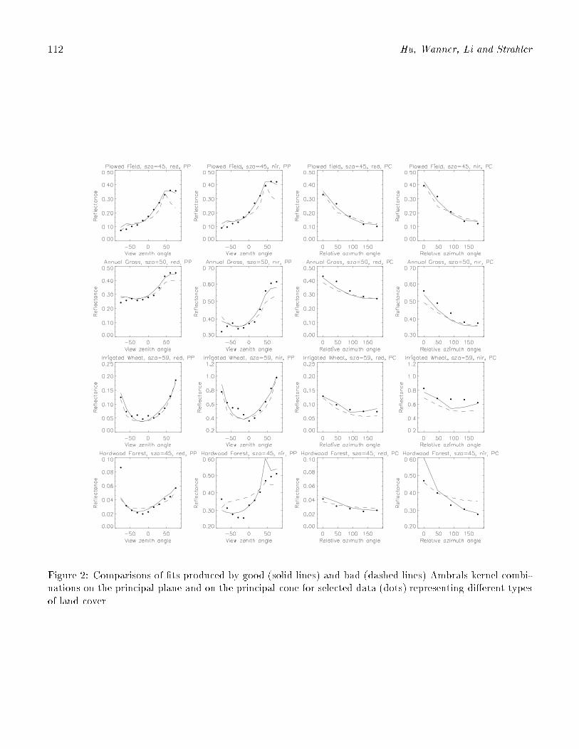
112 Hu, Wanner, Li and Strahler
Figure 2: Comparisons of �ts produced by good (solid lines) and bad (dashed lines) Ambrals kernel combi-nations on the principal plane and on the principal cone for selected data (dots) representing di�erent typesof land cover.

Validation of kernel-driven BRDF models 113
Figure 3: Modeled versus observed re ectances in the red and near-infrared for di�erent types of land cover(barren, forest, broadleaf crops, grass-like). The numbers given in each panel are the correlation coe�cientin the red and in the near-infrared bands, respectively.
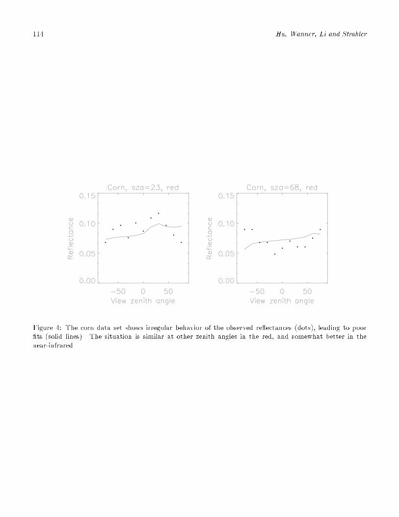
114 Hu, Wanner, Li and Strahler
Figure 4: The corn data set shows irregular behavior of the observed re ectances (dots), leading to poor�ts (solid lines). The situation is similar at other zenith angles in the red, and somewhat better in thenear-infrared.

Validation of kernel-driven BRDF models 115
Figure 5: Modeled versus observed re ectances in the red and near-infrared for di�erent types of land cover(top two rows: sparse vegetation; bottom three rows: dense vegetation) and for a 3-parameter model (left)and a 4-parameter model (right) where the Hapke-kernel for multiple scattering was added. The numbersgiven in each panel are the correlation coe�cient in the red and in the near-infrared bands, respectively.Note that �ts improve for the dense vegetation.
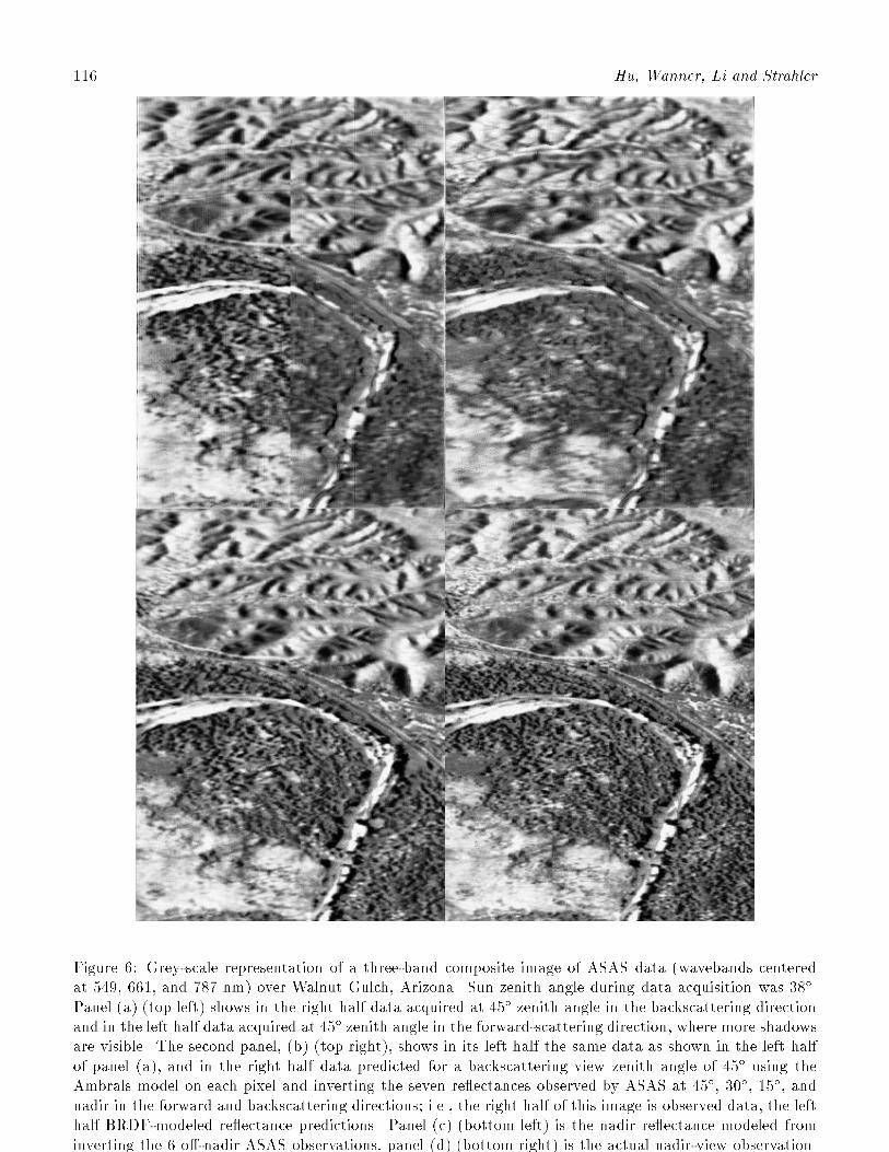
116 Hu, Wanner, Li and Strahler
Figure 6: Grey-scale representation of a three-band composite image of ASAS data (wavebands centeredat 549, 661, and 787 nm) over Walnut Gulch, Arizona. Sun zenith angle during data acquisition was 38�.Panel (a) (top left) shows in the right half data acquired at 45� zenith angle in the backscattering directionand in the left half data acquired at 45� zenith angle in the forward-scattering direction, where more shadowsare visible. The second panel, (b) (top right), shows in its left half the same data as shown in the left halfof panel (a), and in the right half data predicted for a backscattering view zenith angle of 45� using theAmbrals model on each pixel and inverting the seven re ectances observed by ASAS at 45�, 30�, 15�, andnadir in the forward and backscattering directions; i.e., the right half of this image is observed data, the lefthalf BRDF-modeled re ectance predictions. Panel (c) (bottom left) is the nadir re ectance modeled frominverting the 6 o�-nadir ASAS observations, panel (d) (bottom right) is the actual nadir-view observation.

Retrieval Accuracies of BRDF and Albedo 117
APPENDIX B:
RETRIEVAL ACCURACIES OF BRDF AND ALBEDO FROM EOS-
MODIS ANDMISR ANGULAR SAMPLING (PAPER BYWANNER)
118 Wanner
Draft Manuscript (Nov. 96): to be revised and submitted to JGR
Retrieval Accuracies of BRDF and Albedo
from EOS-MODIS and MISR Angular Sampling
Wolfgang Wanner
Center for Remote Sensing and Department of Geography, Boston University, Boston, MA, USA
Abstract. This paper reports expected accuracies of bidirectional re ectance and albedo retrievals fromthe angular sampling provided by NASA's upcoming MODIS and MISR sensors on the EOS-AM-1 satelliteplatform. A numerical discrete ordinates method radiative transfer model by Myneni is used to simulatecombined MODIS and MISR angular sampling as a function of latitude and time of year for six di�erentBRDF types (land cover types) in the red and near-infrared wavebands. These simulated observations arethen inverted using three di�erent simple BRDF models scheduled for use in the future operational MODISand MISR BRDF/Albedo Products:the reciprocal Ambrals, the modi�ed RPV, and the modi�ed WalthallBRDF models. Bidirectional re ectance and albedo retrievals are studied not only at the mean solar zenithangle of observation, but extrapolated to arbitrary other sun zenith angles as well. The in uence of lossof observations to clouds is also examined. Results show that albedo may be retrieved with 2 to 8 percentmedian accuracy using either the Ambrals or the modi�ed RPV model for any solar zenith angle for anyMODIS/MISR sampling, and that the accuracy of predicted nadir-view re ectance is also mostly within a 10percent error margin. The Ambrals model may be slightly more accurate with respect to the forward modelused. The empirical modi�ed Walthall model clearly performs worse than the two semiempirical models.These results also allow to establish error distribution histograms that may serve for assessing the overallaccuracy to be expected from the planned MODIS BRDF/Albedo Product.
1. Introduction
While the elevated standpoint of a low-Earth orbit permits systematic global remote sensing observationsof great value for monitoring continents and the Earth as a whole, it also brings with it restrictions givenby orbital and instrumental mechanics and the limitations of operating an instrument remotely in space.It is of great interest for the assessment of remote sensing missions to determine the accuracy with whichparameters of interest may be retrieved from space. This paper discusses the accuracy to be expected forbidirectional re ectance distribution function (BRDF) and albedo retrieval from the Moderate ResolutionImaging Spectroradiometer (MODIS) and the Multi-Angle Imaging Spectroradiometer (MISR), two instru-ments to be launched on the EOS-AM-1 platform in mid-1998 that are central to NASA's Earth ObservingSystem (EOS) (Running et al., 1994; Diner et al., 1991).
In focusing on BRDF and albedo, this paper studies two parameters that quantify the directional re- ectance characteristics of the Earth's surface, which is the lower boundary for atmospheric transfer ofradiation. BRDF and albedo are consequently of relevance for precise determinations of the Earth's radia-tion budget, climate simulations and atmospheric correction. Other applications are in angular normalizationof images, land cover classi�cation and cloud detection. Besides shedding some light onto the more generalquestion of how e�ectively BRDF and albedo may be derived from space-based remote sensing measurements,this study also is intended to provide much-needed accuracy predictions and error distribution histograms
Retrieval Accuracies of BRDF and Albedo 119
for BRDF and albedo retrievals from MODIS and MISR observations. Such retrievals are to be performedfor the operational BRDF/Albedo standard data product that will be produced routinely from EOS databy the MODIS project (Strahler et al., 1996; Wanner et al., 1997).
The following section 2 outlines the experimental plan and gives details on its components. Sampleresults for BRDF retrieval are presented in section 3, sample results for albedo retrieval in section 4. OverallBRDF and albedo retrieval accuracies are detailed statistically in section 5, which is followed by a discussionand conclusions in section 6.
2. The Experimental Plan
2.1. Outline of the experimental plan
The study was conducted as follows. The orbital simulation tool Xsatview (Barnsley et al., 1994) was used togenerate simulated MODIS and MISR viewing and illumination geometries for di�erent geographic latitudesof observation and days of the year. For each of the observation geometries generated, a discrete ordinatesmethod radiative transfer code (Myneni et al., 1992) was used to compute simulated observations of thebidirectional surface re ectance for six distinct BRDF types resembling six di�erent land cover types in thered and the near-infrared (NIR) wavebands. These were then inverted using three di�erent semiempiricalor empirical BRDF models that are slated for use in operational BRDF/albedo products. These are theAmbrals kernel-driven BRDF model (Wanner et al., 1995, 1997), the Rahman-Pinty-Verstraete model (RPV)(Rahman et al., 1993) in a form modi�ed by Martonchik (Engelsen et al., 1996), and the empirical modi�edWalthall model (Walthall et al., 1985; Nilson and Kuusk, 1989). The �rst and last are to be used for theMODIS BRDF/Albedo Product (which also uses MISR data) (Strahler et al., 1996, Wanner et al., 1997),the second for the MISR Surface Product that includes BRDF and albedo parameters (Diner et al., 1996,Martonchik, 1997).
The BRDF model parameters resulting from the inversions conducted allow reconstruction of the fullBRDF and calculating directional-hemispherical and bihemispherical albedo. The di�erent sampling geome-tries studied represent inversions of the six di�erent BRDF (landcover) types under changing sparse angularsampling, these changes being given by changes in the latitude and time of year of the satellite observations.Any variations in the re ectances and/or albedos found in these experiments for any of the land cover typesare consequently due alone to changes in the angular distribution of samples, everything else having beenkept constant. They re ect the capability of the di�erent models to interpolate and extrapolate the BRDFobserved, given the angular sampling available from observations from space. For example, sampling closeto the principal plane may allow a more reliable reconstruction of the BRDF observed than sampling closeto the cross-principal plane. Sampling at large solar zenith angles may lead to more problems in the infer-ence than at small solar zenith angles since the approximations made in the BRDF models mostly becomequestionable at very large zenith angles. Additionally, one BRDF model may be superior to another in itsability to correctly infer realistic BRDFs from incomplete angular sampling.
The investigation of this problem consists of two parts. First, bottom-line accuracies of BRDF and albedoretrievals need to be determined, which are given by the accuracies achievable in the absence of any otherconfounding factors such as clouds, atmosphere and noise. Consequently, BRDF model inversion is studiedin this paper assuming angular sampling from MODIS and MISR without loss of observations to cloud coverand assuming perfect atmospheric correction of observations (i.e., no atmosphere). Also, the observationsare assumed not to be noisy, although some residual noise from the discreteness of the forward-modelingscheme used is present. In this way, the errors found will represent problems with angular sampling geometryonly. Given the models used, retrievals can never be expected to be better than what is found under suchconditions.
A second part of the overall investigation, currently in progress, is required to establish how these baseline

120 Wanner
accuracies will change given uncertainties in the aerosol optical depth and atmospheric correction, loss ofobservations to cloud cover, and the presence of possibly noisy data. When judging the results of thosestudies, however, it will be essential to know what the accuracies achievable under optimal conditions are, ifindividual sources of error are to be separated. The needed baseline accuracies are reported here. However,some results on the impact of loss of observations to cloud cover are given in section 5. Indications are thatwith MODIS and MISR sampling, the accuracies remain about the same even in the presence of cloud cover,making the results derived in this study rather general.
The e�ect of noisy data on BRDF and albedo retrieval using MODIS and MISR angular sampling isbeing reported elsewhere (Wanner et al., 1996; Lewis and Wanner, 1997).
2.2. MODIS and MISR Angular Sampling
The EOS-AM-1 platform carrying MODIS and MISR will be placed into a polar orbit with a 10:30 a.m.equatorial crossing time. The orbital two-repeat cycle is 16 days, which is also the time resolution at whichthe global MODIS BRDF/Albedo Product will be routinely produced.
The viewing geometries of the two instruments used in generating this product complement each other.Whereas MISR is an along-track imager, MODIS scans across-track. In 16 days, MISR observations willhave been made that cut across the viewing hemisphere at an approximately constant azimuth relativeto the solar plane and are close to perpendicular to a similar cut provided by MODIS observations. Theazimuth angles found depend on the latitude and the time of year. This setup ensures a good coverage ofthe viewing hemisphere when data from the two instruments are used jointly. This applies even to caseswhere some observations are lost due to cloud cover. Coverage of the solar hemisphere is more problematic,as the solar zenith angle for MODIS and MISR observations will vary only slightly in each 16-day period,but vary strongly between latitudes.
MODIS BRDF and albedo will be derived in seven spectral bands ranging from 0.47 �m to 2.13 �m,with MISR data being available between 0.43 �m and 0.87 �m. The spatial resolution of the product willbe one kilometer, with good geolocation of each pixel ensured by a greater spatial resolution of the originaldata used in building a multiangular database. This slight degradation of the spatial resolution in producingthe product is essential in regions with heterogeneous land covers.
MODIS and MISR viewing and illumination geometries were simulated using orbital simulation softwarecalled Xsatview (Barnsley et al., 1994). Observation geometries are represented approximately due tosome simpli�cations made, but are su�ciently accurate for the purposes of this study. Observations weresimulated at 9 di�erent latitudes between 80 degrees northern and 80 degrees southern latitude, and forsolar positions corresponding to every third 16-day time period throughout the year (8 periods). Of the 72resulting sampling scenarios, 60 provide observations with the sun above the horizon. Observations with sunzenith angles larger than 75 degrees were discarded since this will also be the case in MODIS atmosphericcorrection processing.
2.3. BRDF Forward Modeling from DOM/RTCODE
Forward BRDF Modeling was carried out using a discrete ordinates code provided by Myneni (Myneni etal., 1992) that solves the radiative transfer equations of light scattering in structured vegetation canopiesand also takes geometrical shadowing e�ects into account. This code, used in version available in early1996 (here called DOM/RTCODE), is written to predict the BRDFs of six land cover types with distinctcharacteristics. These so-called biomes are: grasses and cereal crops (biome 1); semi-arid shrublands (biome2); broadleaf crops (biome 3); savanna, which is a grassy understory with a sparse overstory of trees (biome4); broadleaf forest (biome 5); and needleleaf forest (biome 6).
The parameters for each biome simulation, between 17 and 32 depending on the case, were set to realistic
Retrieval Accuracies of BRDF and Albedo 121
values. For all biomes, the soil background was assumed to be Lambertian and have a red hemisphericalre ectance of 0.1 and a near-infrared hemispherical re ectance of 0.2. The fraction of direct illuminating ra-diation was assumed to be 0.8, not so much to simulate di�use skylight (which in remote sensing applicationswould have been corrected for in atmospheric correction) but to make the BRDFs less ideal in terms of thecrispness of features produced by idealistic mathematical models but not found in a natural situation. Leafoptical properties were generally taken to be similar across biomes. Red hemispherical leaf re ectance was0.076, leaf hemispherical transmittance 0.042. The corresponding values in the near-infrared were 0.52 and0.41. Stem and branch optical properties were mostly similar to the leaf properties but sometimes chosento be less transparent.
The grassland biome had a leaf area index (LAI) of 2.0 with a canopy height of 0.8 m. The leaf normalinclination was assumed erectophile. The shrubs in the semi-arid shrubland were simulated to have a LAI of2.0 with a ground cover of 50 percent, that is the plot LAI was 1.0. The height of the shrubs was assumedto be 4 m, sitting on the ground, and the leaf angle distribution to be uniform. The broadleaf crop canopywas characterized as having a LAI of 3.0 with a stem and branch area index of 0.6. Ground cover wasassumed to be 80 percent, resulting in a plot LAI of 2.4. Stand height was taken to be 1.25 m, the leaf angledistribution to be uniform and the stem normal orientation vertical.
The savanna biome type was characterized as having a 20 percent tree cover, the trees being 5 m highwith crowns of 2 m length. The LAI was taken to be 4.0 with a uniform leaf angle distribution. Theunderstory of grass was assumed to be 1.0 m high and erectophile with an LAI of 2.0, resulting in a plotLAI of 2.8. The broadleaf forest is characterized by a 90 percent ground cover consisting of trees 10 m high,with crowns measuring 4 m in height and 3m in diameter. The branch/stem orientation and the leaf angledistribution are uniform. LAI is 5.5. The understory is 1 m high, has a uniform leaf angle distribution anda LAI of 1.0. Total stand LAI is 5.95. The needleleaf forest, �nally, has an 80 percent ground cover witha tree leaf area index of 2.5. The trees are 10 m high with crowns measuring 4 m in height and 2 m indiameter, the shoots having a uniform leaf angle distribution but the needles showing clumping. The anglebetween needle and shoot is 49 degrees. As before, the understory has a uniform leaf angle distribution andan LAI of 1.0 with a plant height of 1 m. Plot LAI is 3.0.
Bidirectional re ectances were generated from the DOM/RTCODE for MODIS and MISR viewing andillumination geometries, and the corresponding directional-hemispherical and bihemispherical albedos de-termined. Since two wave bands, red and near-infrared, were simulated, a total of 12 BRDFs was sampledin 60 di�erent ways as a function of latitude and day of year, resulting in 720 observations of a BRDF fromwhich to attempt a retrieval of BRDF and albedo.
Generally, the BRDFs produced by DOM/RTCODE were satisfactory in the angle ranges mainly ofinterest. Biomes 1 and 5 displayed no obvious problems. For biome 3, the discretization of the schemewas visible for close-to-nadir solar zenith angles. Biomes 2 and 5 displayed small residual irregularities atnadir view zenith for small solar zenith angles, mostly in the red band, but these were not deemed to beoverly problematic for the current study. Biome 4 displayed some noise in the backscattering direction forlarge viewing and solar zenith angles, but again this was not deemed critical. Di�erences in BRDF shapebetween biomes consisted mainly of the steepness of the bowl, the properties of the hotspot region, and themagnitude of the re ectances. All in all, however, the BRDFs for the six biomes are somewhat similar intheir overall appearance. This may either be due to similarities in the modeling used for the di�erent biometypes, or to the fact that natural BRDFs are more similar than expected when both shadowing and radiativetransfer-type e�ects are both combined realistically in the same model.
2.4. Inverse Modeling Using Simple BRDF Models
Three di�erent BRDF models were used for inverting the simulated MODIS and MISR multiangular ob-servations, the Ambrals BRDF model (Wanner et al., 1995, 1997) in a slightly modi�ed form, the modi�ed

122 Wanner
BRDF model by Rahman et al. (1993), commonly called RPV, and the modi�ed Walthall model (Walthallet al., 1985; Nilson and Kuusk, 1989). These models were chosen because they will be used for generatingBRDF and albedo from the MODIS and MISR instruments and probably are the only BRDF models cur-rently feasible for large-scale operational applications. The latter is mainly due to their small number ofparameters and the fact that they may be inverted without recourse to iterative numerical inversion schemes,which cannot be a�orded in global kilometer-scale processing given currently achievable computer power.A model similar in approach to the Ambrals model is also used for BRDF and albedo modeling from dataacquired by the polarization and directionality of the earth's radiation (POLDER) instrument (Deschampset al., 1994; Leroy et al., 1997).
The Ambrals model and the RPV model are semiempirical models based on somewhat di�erent philoso-phies. The Ambrals model is formulated as a sum of two expressions, one that characterizes the shadowcasting of discrete ground objects as determined by inter-object gaps, and one that characterizes volumescattering from homogeneously distributed scattering elements as determined by intra-canopy gaps (Roujeanet al., 1992). Expressions for these two components, geometric and volume scattering, are derived througha series of simplifying approximations from physical BRDF theories (Wanner et al., 1995), most notably aradiative transfer theory taken from Ross (1981) and the Li-Strahler geometric-optical mutual shadowingmodel (Li and Strahler, 1992). In inversion, the relative contributions of volume and geometric scattering,and an isotropic constant, are retrieved. These may be interpreted to re ect either the sub-resolution mix-ture of land cover types that are dominated by either volume or geometric scattering, or to quantify therespective scattering contributions from a single type of land cover.
For volume and geometric scattering, the Ambrals model provides a choice of two alternate mathematicalexpressions each, called kernels, representing di�erent types of scattering due to di�erent types of approxima-tions made. For volume scattering, the two kernels available describe canopies with high or low e�ective leafarea index (Ross-thin, Ross-thick kernels), for geometric scattering they model sparse and dense canopies(Li-sparse, Li-dense kernels). In this study, the kernels to be used for each inversion were chosen such thata minimum root mean square absolute error between modeled and observed re ectances is achieved (Hu etal., 1996, 1997; Wanner et al., 1995, 1997). The crown structural parameters used in the Li kernels were:sparse kernel, crown height to width ratio 1.0, dense kernel 2.5; both kernels, height to the center of crown2.0, resulting in a lower sparse canopy than dense canopy. These values were chosen because they are likelyto also be used in operational BRDF processing for MODIS.
One change was made to the published version of the Ambrals model Li kernels (Wanner et al., 1995).The original Li-Strahler BRDF model was formulated for a �xed angle of illumination (Li and Strahler, 1992).The angle dependence of the scene component re ectances was not part of the modeling conducted. Schaafand Strahler (1994) and Schaaf, Li and Strahler (1994), however, gave an expression for the most importantof these component signatures, the re ectance of the sunlit crowns. This was modeled as following the ratioof actual to projected sunlit crown area. In deriving the geometric Li kernels for the Ambrals model, initiallya constant sunlit crown component re ectance was assumed for simplicity. This, however, led to the kernelsbeing not reciprocal with respect to an exchange of sun and viewing angle. The version of Ambrals used inthis paper resolves this situation. The sunlit crown component re ectance C was modeled in approximationas C= cos(�s), where cos(�s) is the solar zenith angle. This also makes the Li kernels reciprocal.
The RPV BRDF model, on the other hand, is based on a somewhat more empirical approach thatquanti�es the qualitative features of BRDF shape. Three functions that each govern one distinct aspect ofthe BRDF shape are multiplied by each other to form the model (Rahman et al., 1993). These are a modi�edMinnaert term, used to describe the bowl-shape of the BRDF, a Henyey-Greenstein function describing theskew in the BRDF between forward and backscattering, and a hotspot term. Like the Ambrals model, theRPV model has three parameters, quantifying the overall intensity of the re ectance, the strength of theanisotropy, and the relative amount of forward and backward scattering. This provides for a wide varietyof shapes as may typically be found for observed BRDFs (Engelsen et al., 1996). The model is nonlinear,
Retrieval Accuracies of BRDF and Albedo 123
which is undesirable for reasons of computing resources in operational applications. Therefore, the modelwas modi�ed by Martonchik (Engelsen et al., 1996) to be semi-linear, requiring only a few simple iterationsfor inversion. This modi�ed form, slated for use in MISR data processing, was used in this study.
The modi�ed Walthall model (Walthall et al., 1985; Nilson and Kuusk, 1989), �nally, is a purely em-pirical model with four parameters based on very simple expressions containing the view and illuminationangles. The attraction of this model is mainly that it manages to capture the main features of BRDF shapewhile being very simple (albedo, for example, can be calculated analytically). However, it is interesting toinvestigate whether the fact that the Ambrals and the RPV model are based on a more physical reasoningthan the Walthall model leads to smaller errors for these models when extrapolating BRDF inversion resultsto angles where no observations were acquired, for example a di�erent sun angle. As will be seen later, theempirical model is indeed found to be doing worse than the two semiempirical models in this respect despitethe fact that it has one more free parameter.
In keeping with the stated goal of deriving bottom-line accuracies, models were inverted by minimizingthe error function separately in the red and the near-infrared band, not simultaneously. There is an inherentproblem with respect to coupled BRDF and albedo retrieval in the two principal ways in which error in thered and in the near-infrared band can be traded o�. If the combined absolute error is to be minimized, thelarger re ectances are modeled relatively more accurately than the smaller ones. This provides for a preciseretrieval of albedo, which is dominated by the large re ectances, but is less desirable in the retrieval of redband BRDFs. A relative error measure, on the other hand, allows better modeling of small re ectances, e.g.,a better BRDF retrieval in the red band, but by the same token allows larger deviations in large re ectances,which translate into undesired larger errors in albedo. This contradiction in the requirements for the errorfunction with respect to BRDF and albedo retrieval is not basically resolvable. In this study, absolute errorwas minimized, but separately in each band, avoiding de�nition of a tradeo� between errors in the largernear-infrared re ectance values and the smaller ones in the red band, and allowing to establish the sought-forbottom-line accuracies.
3. Examples of BRDF Retrievals
Since albedo is derived through integration of the BRDF, the �rst concern is for accurate retrieval of theBRDF. Figure 1 shows MODIS and MISR sampling at di�erent latitudes for a 16-day period starting day ofthe year 96, in April. Obviously, sampling of the viewing hemisphere is rather reasonable, and even loss ofobservations to clouds should not regularly impact the angle coverage in a decisive way. At some latitudes,though, the principal plane is not being sampled by either instrument. This could be a problem in somecases since BRDFs tend to be more dissimilar on the principal plane than on the cross-principal plane.
The main shortcoming of the angular sampling available, however, is in the solar angle hemisphere. Ateach latitude the range of solar zenith angles covered is only very small, usually not more than 10 degrees.But the main concern is that the mean solar zenith angle of observations varies strongly from one latitudeto another, covering most of the full zenith angle range. In other words, the BRDF as a function of viewingangle will be well determined at solar angles that vary with latitude, and with time of year.
The main question with respect to BRDF retrieval consequently is whether the retrievals achievable at thesolar angle of observation may safely be extrapolated to other solar zenith angles, allowing for example thestandardization of surface re ectances not only to a common viewing geometry but also to a common solargeometry. The angles most preferred for such a standardization would be nadir viewing and illuminationsince under such conditions the understory will be most visible and no shadows will contaminate the scene.However, structural information to be derived from the BRDF is best obtained at o�-nadir angles whereshadow characteristic may be determined. O�-nadir angles also determine albedo.
Consequently, the following rather severe test is applied to BRDF retrieval. Inversion results are in-
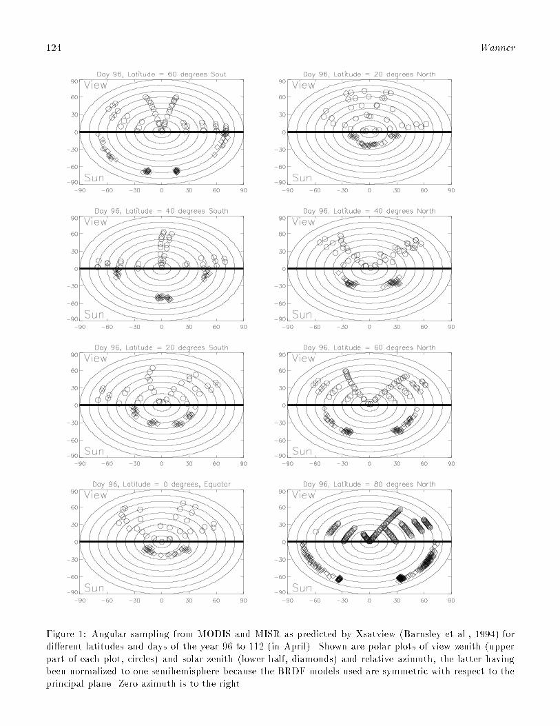
124 Wanner
Figure 1: Angular sampling from MODIS and MISR as predicted by Xsatview (Barnsley et al., 1994) fordi�erent latitudes and days of the year 96 to 112 (in April). Shown are polar plots of view zenith (upperpart of each plot, circles) and solar zenith (lower half, diamonds) and relative azimuth, the latter havingbeen normalized to one semihemisphere because the BRDF models used are symmetric with respect to theprincipal plane. Zero azimuth is to the right.
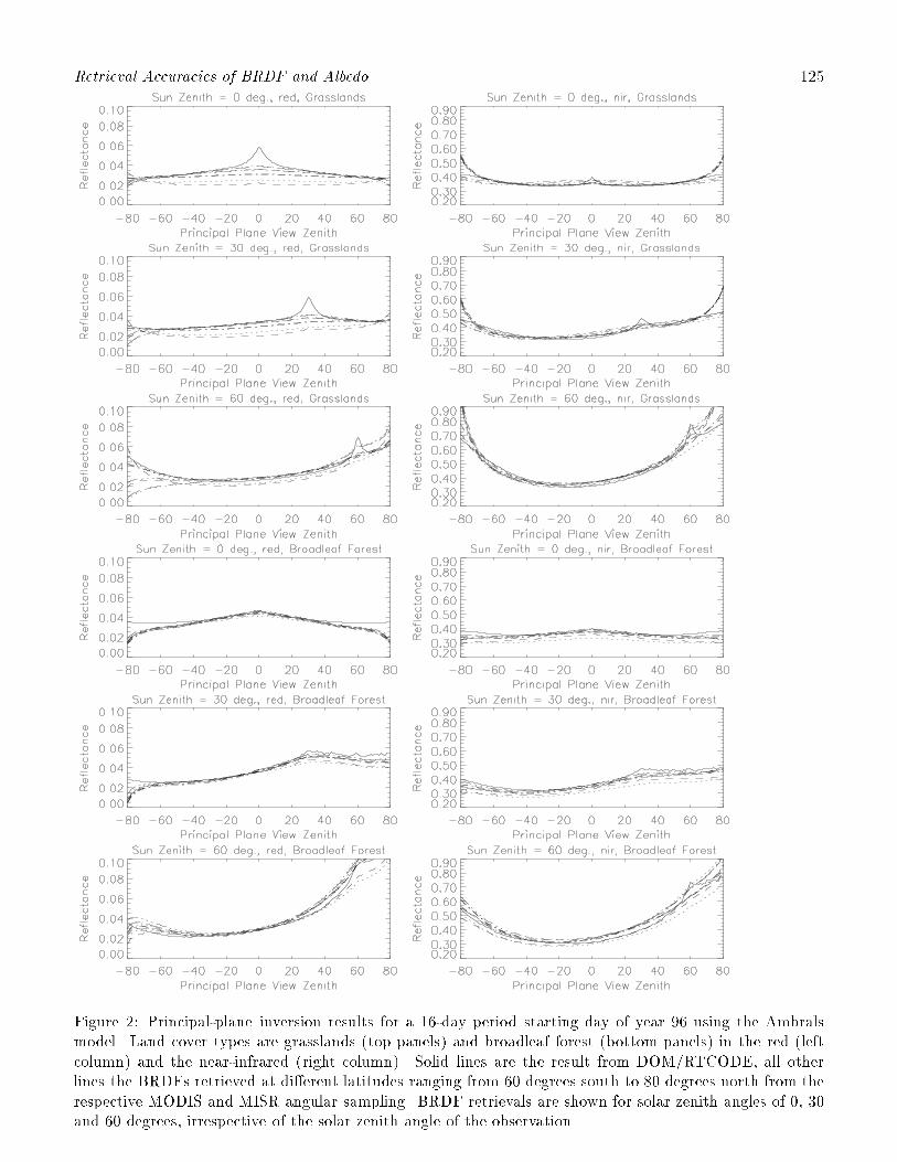
Retrieval Accuracies of BRDF and Albedo 125
Figure 2: Principal-plane inversion results for a 16-day period starting day of year 96 using the Ambralsmodel. Land cover types are grasslands (top panels) and broadleaf forest (bottom panels) in the red (leftcolumn) and the near-infrared (right column). Solid lines are the result from DOM/RTCODE, all otherlines the BRDFs retrieved at di�erent latitudes ranging from 60 degrees south to 80 degrees north from therespective MODIS and MISR angular sampling. BRDF retrievals are shown for solar zenith angles of 0, 30and 60 degrees, irrespective of the solar zenith angle of the observation.
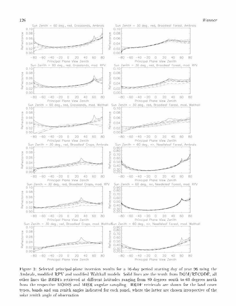
126 Wanner
Figure 3: Selected principal-plane inversion results for a 16-day period starting day of year 96 using theAmbrals, modi�ed RPV and modi�ed Walthall models. Solid lines are the result from DOM/RTCODE, allother lines the BRDFs retrieved at di�erent latitudes ranging from 80 degrees south to 60 degrees northfrom the respective MODIS and MISR angular sampling. BRDF retrievals are shown for the land covertypes, bands and sun zenith angles indicated for each panel, where the latter are chosen irrespective of thesolar zenith angle of observation.
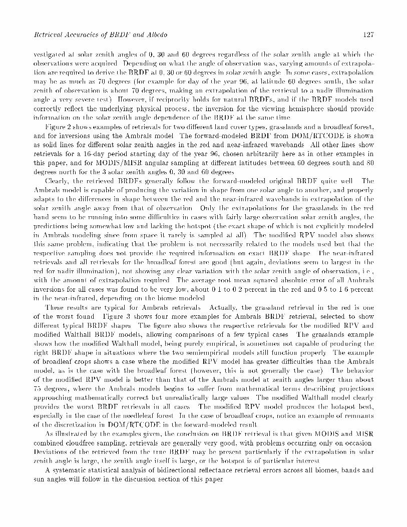
Retrieval Accuracies of BRDF and Albedo 127
vestigated at solar zenith angles of 0, 30 and 60 degrees regardless of the solar zenith angle at which theobservations were acquired. Depending on what the angle of observation was, varying amounts of extrapola-tion are required to derive the BRDF at 0, 30 or 60 degrees in solar zenith angle. In some cases, extrapolationmay be as much as 70 degrees (for example for day of the year 96, at latitude 60 degrees south, the solarzenith of observation is about 70 degrees, making an extrapolation of the retrieval to a nadir illuminationangle a very severe test). However, if reciprocity holds for natural BRDFs, and if the BRDF models usedcorrectly re ect the underlying physical process, the inversion for the viewing hemisphere should provideinformation on the solar zenith angle dependence of the BRDF at the same time.
Figure 2 shows examples of retrievals for two di�erent land cover types, grasslands and a broadleaf forest,and for inversions using the Ambrals model. The forward-modeled BRDF from DOM/RTCODE is shownas solid lines for di�erent solar zenith angles in the red and near-infrared wavebands. All other lines showretrievals for a 16-day period starting day of the year 96, chosen arbitrarily here as in other examples inthis paper, and for MODIS/MISR angular sampling at di�erent latitudes between 60 degrees south and 80degrees north for the 3 solar zenith angles 0, 30 and 60 degrees.
Clearly, the retrieved BRDFs generally follow the forward-modeled original BRDF quite well. TheAmbrals model is capable of producing the variation in shape from one solar angle to another, and properlyadapts to the di�erences in shape between the red and the near-infrared wavebands in extrapolation of thesolar zenith angle away from that of observation. Only the extrapolations for the grasslands in the redband seem to be running into some di�culties in cases with fairly large observation solar zenith angles, thepredictions being somewhat low and lacking the hotspot (the exact shape of which is not explicitly modeledin Ambrals modeling since from space it rarely is sampled at all). The modi�ed RPV model also showsthis same problem, indicating that the problem is not necessarily related to the models used but that therespective sampling does not provide the required information on exact BRDF shape. The near-infraredretrievals and all retrievals for the broadleaf forest are good (but again, deviations seem to largest in thered for nadir illumination), not showing any clear variation with the solar zenith angle of observation, i.e.,with the amount of extrapolation required. The average root mean squared absolute error of all Ambralsinversions for all cases was found to be very low, about 0.1 to 0.2 percent in the red and 0.5 to 1.6 percentin the near-infrared, depending on the biome modeled.
These results are typical for Ambrals retrievals. Actually, the grassland retrieval in the red is oneof the worst found. Figure 3 shows four more examples for Ambrals BRDF retrieval, selected to showdi�erent typical BRDF shapes. The �gure also shows the respective retrievals for the modi�ed RPV andmodi�ed Walthall BRDF models, allowing comparisons of a few typical cases. The grasslands exampleshows how the modi�ed Walthall model, being purely empirical, is sometimes not capable of producing theright BRDF shape in situations where the two semiempirical models still function properly. The exampleof broadleaf crops shows a case where the modi�ed RPV model has greater di�culties than the Ambralsmodel, as is the case with the broadleaf forest (however, this is not generally the case). The behaviorof the modi�ed RPV model is better than that of the Ambrals model at zenith angles larger than about75 degrees, where the Ambrals models begins to su�er from mathematical terms describing projectionsapproaching mathematically correct but unrealistically large values. The modi�ed Walthall model clearlyprovides the worst BRDF retrievals in all cases. The modi�ed RPV model produces the hotspot best,especially in the case of the needleleaf forest. In the case of broadleaf crops, notice an example of remnantsof the discretization in DOM/RTCODE in the forward-modeled result.
As illustrated by the examples given, the conclusion on BRDF retrieval is that given MODIS and MISRcombined cloudfree sampling, retrievals are generally very good, with problems occurring only on occasion.Deviations of the retrieved from the true BRDF may be present particularly if the extrapolation in solarzenith angle is large, the zenith angle itself is large, or the hotspot is of particular interest.
A systematic statistical analysis of bidirectional re ectance retrieval errors across all biomes, bands andsun angles will follow in the discussion section of this paper.

128 Wanner
4. Examples of Albedo Retrievals
Integration of the BRDF over the viewing hemisphere gives directional-hemispherical albedo, also calledblack-sky albedo because the BRDF describes the re ectance in the absence of di�use skylight (Strahler etal., 1995; Wanner et al., 1997). Black-sky albedo is a function of solar zenith angle. The double integralover the viewing and illumination hemispheres produces bihemispherical or white-sky albedo, a constantdescribing total average re ectance under isotropic illumination (an approximation perhaps to overcastskies) (Strahler et al., 1995; Wanner et al., 1997). Black-sky and white-sky albedo are important parametersto be derived from remote sensing since they describe average re ectance properties of the surface underdi�erent angles of illumination, and represent the albedos of the extremes of a clean or clear and a stronglyturbid atmospheric condition. Surface albedos directly enter atmospheric correction algorithms and energybudget calculations and are an important driver in climate and weather models. Their global derivation andmapping is one of the goals of NASA's Earth Observing System.
Figure 4 shows black-sky and white-sky albedo retrieval relative errors as a function of latitude for all sixBRDF types (land cover types) studied for di�erent solar zenith angles in the red and the near-infrared, andfor a 16-day period beginning day of the year 96. Retrievals for the mean solar zenith angle of observationare shown in the top two panels, illustrating the relative error made under prevailing illumination conditions.The other panels show retrieval accuracies at solar zenith angles 0, 30 and 60 degrees irrespective of thesolar angle of the observations. White-sky albedo retrieval errors are shown in the bottom panels. Theshaded band marks the plus/minus 10 percent region, within which retrievals ideally should be contained.It is important to note that all variations displayed in this �gure are due to changes in sampling geometryalone. Clearly, a trend of error with latitude is seen, re ecting the changes in angular sampling pattern.
With the exception of some retrievals at latitude 60 degrees south in the red band, and for �ve of thesix biomes studied, nearly all albedos are within a 10 percent margin of relative error. In many cases,especially in the near-infrared, they are well within that margin. Errors in the near-infrared mostly showlittle variation with latitude, indicating robustness against the sampling e�ects occurring. In the red, theretrievals are relatively less stable, owing to the larger sensitivity of a small albedo to errors in re ectance.The retrievals for some biomes at some solar zenith angles are o� by 10 to 30 percent. But still, the bulkof data falls within the 10 percent margin. It is interesting to note that in both bands the retrievals fora solar zenith angle of 30 degrees show less error than the retrievals at the mean solar zenith angle of theobservations. This re ects the fact that the models �t moderate solar zenith angles better than large ones.Results at the prevailing solar zenith angle of observations are worse if that angle is large than when thisresult is extrapolated to a smaller angle. This bodes well for deriving albedo at a standardized, typical solarzenith angle, perhaps at 30 or 45 degrees.
White-sky albedo errors, being dependent on the accurate prediction of black-sky albedo at all solarangles, show in many cases larger errors than the black-sky albedo retrievals at the smaller solar zenithangles. Again, an improvement would be achieved if the model could be altered to �t BRDFs better atlarge zenith angles, but the accuracies achieved are still acceptable in view of the fact that any derivationof white-sky albedo necessarily involves a large amount of extrapolation of data in the absence of goodsampling of the solar hemisphere.
Figure 5 compares Ambrals retrieval accuracies with those for the modi�ed RPV and the modi�edWalthall models for a few selected cases showing typical results. The modi�ed RPV model generally showserror patterns that are very similar to those of Ambrals, i.e., when one model has a problem the otherone does too. This indicates that the problems encountered are based on a lack of required directionalinformation in the angular sampling available, not in an inherent inability of the models to predict betterresults. Individual examples can be found in the full data set where either the Ambrals or the modi�edRPV model are doing better. There is a tendency, however, for modi�ed RPV model retrievals to be moreconsistent in terms of the size of the error produced. The modi�ed Walthall model generally does worse,
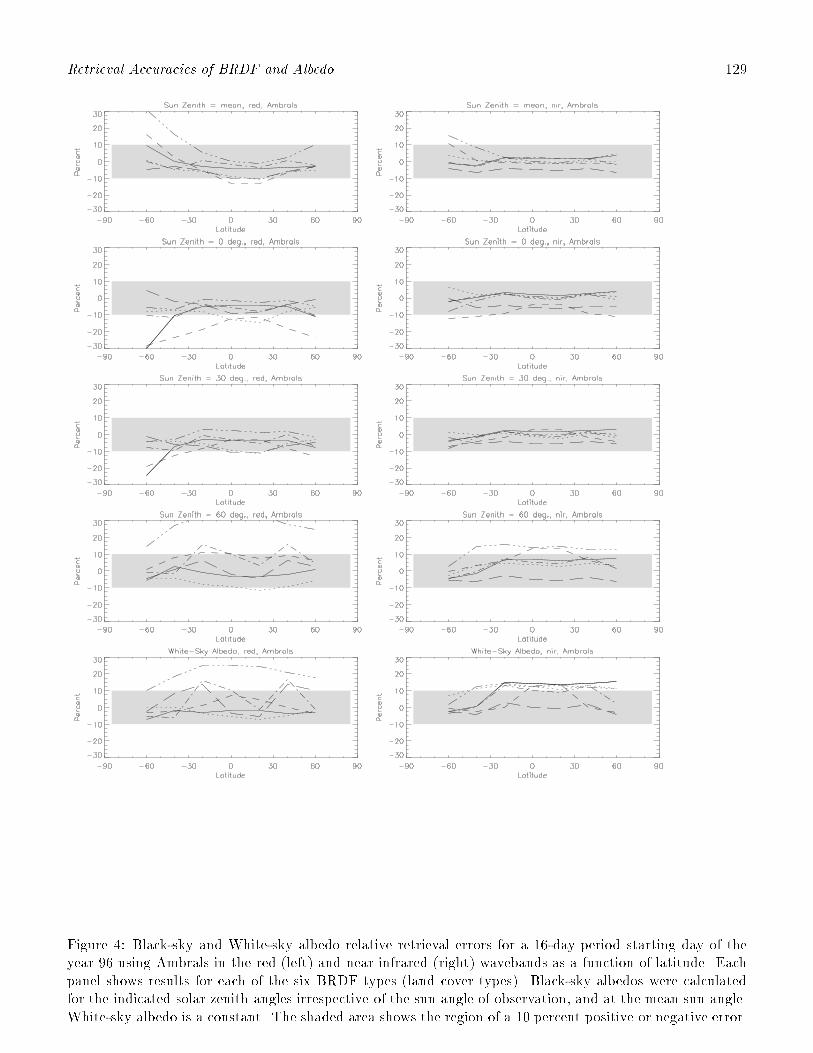
Retrieval Accuracies of BRDF and Albedo 129
Figure 4: Black-sky and White-sky albedo relative retrieval errors for a 16-day period starting day of theyear 96 using Ambrals in the red (left) and near infrared (right) wavebands as a function of latitude. Eachpanel shows results for each of the six BRDF types (land cover types). Black-sky albedos were calculatedfor the indicated solar zenith angles irrespective of the sun angle of observation, and at the mean sun angle.White-sky albedo is a constant. The shaded area shows the region of a 10 percent positive or negative error.
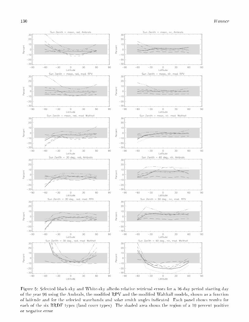
130 Wanner
Figure 5: Selected black-sky and White-sky albedo relative retrieval errors for a 16-day period starting dayof the year 96 using the Ambrals, the modi�ed RPV and the modi�ed Walthall models, shown as a functionof latitude and for the selected wavebands and solar zenith angles indicated. Each panel shows results foreach of the six BRDF types (land cover types). The shaded area shows the region of a 10 percent positiveor negative error.
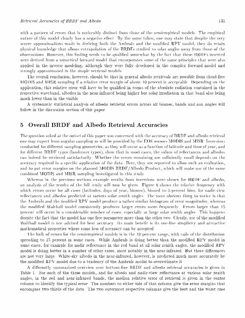
Retrieval Accuracies of BRDF and Albedo 131
with a pattern of errors that is noticeably distinct from those of the semiempirical models. The empiricalnature of this model clearly has a negative e�ect. By the same token, one may state that despite the verysevere approximations made in deriving both the Ambrals and the modi�ed RPV model, they do retainphysical knowledge that allows extrapolation of the BRDFs studied to solar angles away from those of theobservations. However, this �nding needs to be quali�ed somewhat by the fact that these BRDFs invertedwere derived from a numerical forward model that encorporates some of the same principles that were alsoapplied in the inverse modeling, although they were fully developed in the complex forward model andstrongly approximated in the simple retrieval models.
The overall conclusion, however, should be that in general albedo retrievals are possible from cloud-freeMODIS and MISR sampling if a relative error margin of about 10 percent is acceptable. Depending on theapplication, this relative error will have to be quali�ed in terms of the absolute radiation contained in therespective waveband, albedos in the near-infrared being higher but solar irradiation in that band also beingmuch lower than in the visible.
A systematic statistical analysis of albedo retrieval errors across all biomes, bands and sun angles willfollow in the discussion section of this paper.
5. Overall BRDF and Albedo Retrieval Accuracies
The question asked at the outset of this paper was concerned with the accuracy of BRDF and albedo retrievalone may expect from angular sampling as will be provided by the EOS sensors MODIS and MISR. Inversionsconducted for di�erent sampling geometries, as they will occur as a function of latitude and time of year, andfor di�erent BRDF types (landcover types), show that in most cases, the values of re ectances and albedoscan indeed be retrieved satisfactorily. Whether the errors remaining are su�ciently small depends on theaccuracy required in a speci�c application of the data. Here, they are reported to allow such an evaluation,and to put error margins on the planned MODIS BRDF/Albedo Product, which will make use of the samecombined MODIS and MISR sampling investigated in this study.
Whereas in the previous sections example results from inversions were shown for BRDF and albedo,an analysis of the results of the full study will now be given. Figure 6 shows the relative frequency withwhich errors occur for all cases (latitudes, days of year, biomes), binned to 5-percent bins, for nadir-viewre ectances and albedos predicted at various solar zenith angles. The most obvious thing to notice is thatthe Ambrals and the modi�ed RPV model produce a rather similar histogram of error magnitudes, whereasthe modi�ed Walthall model consistently produces larger errors more frequently. Errors larger than 15percent still occur in a considerable number of cases, especially at large solar zenith angles. This happensdespite the fact that the model has one free parameter more than the other two. Clearly, use of the modi�edWalthall model is not advised for best accuracy. Its main bene�t is its one-line simplicity and attractivemathematical properties where some loss of accuracy can be accepted.
The bulk of errors for the semiempirical models is in the 10 percent range, with tails of the distributionspreading to 15 percent in some cases. While Ambrals is doing better than the modi�ed RPV model insome cases, for example for nadir re ectance in the red band at all solar zenith angles, the modi�ed RPVmodel is doing better in a number of other cases, most notably in the near-infrared. But these di�erencesare not very large. White-sky albedo in the near-infrared, however, is predicted much more accurately bythe modi�ed RPV model due to a tendency of the Ambrals model to overestimate it.
A di�erently summarized overview over bottom-line BRDF and albedo retrieval accuracies is given inTable 1. For each of the three models, and for albedo and nadir-view re ectance at various solar zenithangles, in the red and near-infrared bands, the median relative error of retrieval is given in the centercolumn to identify the typical error. The numbers to either side of that column give the error margins thatencompass two thirds of the data. The two outermost respective columns give the best and the worst case

132 Wanner
Figure 6: Histograms of the distribution of relative errors of retrieval for nadir-view re ectance and albedofor the Ambrals (solid line), modi�ed RPV (dashed line) and modi�ed Walthall model (dotted line) in thered and near-infrared. Histograms are based on data from all latitudes, all six BRDF types (biomes) and alldays of the year tested. Results were obtained for the solar angles indicated, irrespective of the solar zenithangles of observation. Relative frequency is shown based on bins with a width of 5 percent.

Retrieval Accuracies of BRDF and Albedo 133Table 1: Predicted Retrieval Accuracies: All Latitudes, Times of Year and Biome Types. Median Error,Two-Thirds of Cases Range, and Best and Worst Error Found.
Model Band Solar Albedo Nadir Re ectanceZenith Percentage of Data Percentage of DataAngle 0/6 1/6 3/6 5/6 6/6 0/6 1/6 3/6 5/6 6/6
Ambrals red �s = 0 0.0 3.7 7.5 16.0 33.2 0.0 1.1 5.5 28.7 50.1�s = 30 0.0 2.5 4.8 11.0 24.2 0.0 1.2 5.4 14.5 41.0�s = 60 0.0 2.3 6.0 16.0 42.6 0.0 2.1 7.9 11.9 21.8h�siobs 0.0 1.9 4.3 9.6 39.0 0.0 0.9 3.2 8.1 13.6R�s 0.0 1.4 5.3 14.2 31.4
nir �s = 0 0.0 0.8 3.0 6.4 17.3 0.0 0.8 6.1 13.9 38.3�s = 30 0.0 0.6 2.5 5.4 14.4 0.0 1.3 4.6 8.8 28.7�s = 60 0.0 2.5 5.4 8.8 19.1 0.0 1.2 5.2 9.6 15.2h�siobs 0.0 0.5 2.0 4.9 19.9 0.0 0.7 3.3 6.6 13.2R�s 0.0 1.6 8.1 13.4 16.7
red �s = 0 0.0 1.6 4.8 11.6 33.2 0.0 1.0 5.9 17.8 50.1+nir �s = 30 0.0 1.2 3.7 7.6 24.2 0.0 1.2 4.9 11.6 41.0
�s = 60 0.0 2.4 5.7 12.6 42.6 0.0 1.5 6.5 11.2 21.8h�siobs 0.0 0.9 3.1 6.7 39.0 0.0 0.8 3.3 7.1 13.6R�s 0.0 1.5 6.0 13.8 31.4
modi�ed red �s = 0 0.0 2.2 6.3 15.4 43.2 0.0 2.4 7.2 28.2 59.8RPV �s = 30 0.0 1.8 5.6 11.4 33.6 0.0 1.6 6.6 19.7 48.6
�s = 60 0.0 2.2 7.9 14.1 32.6 0.0 3.8 10.3 14.6 23.7h�siobs 0.0 1.2 5.1 8.3 39.6 0.0 1.1 3.6 8.8 17.5R�s 0.0 3.1 7.4 13.1 27.7
nir �s = 0 0.0 1.3 4.6 8.6 25.5 0.1 2.2 5.5 11.5 34.2�s = 30 0.0 0.6 3.4 7.7 23.3 0.0 1.3 2.8 7.0 29.9�s = 60 0.0 1.9 4.5 6.7 19.7 0.0 1.4 5.3 10.3 15.8h�siobs 0.0 0.4 2.5 5.5 24.0 0.0 0.9 2.3 5.1 15.4R�s 0.0 1.4 3.9 6.7 18.3
red �s = 0 0.0 1.7 5.5 12.8 43.2 0.0 2.2 6.1 20.3 59.8+nir �s = 30 0.0 1.2 4.8 9.8 33.6 0.0 1.4 4.3 14.1 48.6
�s = 60 0.0 2.0 5.3 11.7 32.6 0.0 2.0 7.7 12.9 23.7h�siobs 0.0 0.6 3.2 7.2 39.6 0.0 1.0 2.7 6.6 17.5R�s 0.0 2.0 5.4 10.6 27.7
modi�ed red �s = 0 0.2 3.0 10.6 48.6 303.4 0.0 3.0 12.0 53.1 293.5Walthall �s = 30 0.0 3.8 9.0 42.5 270.4 0.1 2.0 9.8 55.6 308.6
�s = 60 0.1 8.1 26.5 41.6 163.6 0.0 4.3 13.5 43.1 257.1h�siobs 0.0 2.9 6.7 11.8 46.9 0.0 2.3 8.7 35.8 131.2R�s 0.4 8.5 23.7 38.6 179.0
nir �s = 0 0.0 2.6 9.2 35.2 180.7 0.0 6.7 16.0 51.2 290.9�s = 30 0.0 1.8 7.2 26.6 143.7 0.1 7.3 19.0 54.1 245.0�s = 60 0.1 5.0 13.9 21.8 62.2 0.0 4.1 13.5 40.1 145.1h�siobs 0.0 1.1 3.5 7.4 31.6 0.1 3.4 18.4 33.7 76.1R�s 0.3 4.9 11.8 17.3 74.8
red �s = 0 0.0 2.8 9.8 42.6 303.4 0.0 4.9 13.5 53.1 293.5+nir �s = 30 0.0 2.6 8.2 35.4 270.4 0.1 3.2 14.5 54.2 308.6
�s = 60 0.1 6.2 18.1 34.7 163.6 0.0 4.3 13.5 40.5 257.1h�siobs 0.0 1.6 5.0 10.2 46.9 0.0 3.0 14.5 34.8 131.2R�s 0.3 6.1 14.9 33.7 179.0
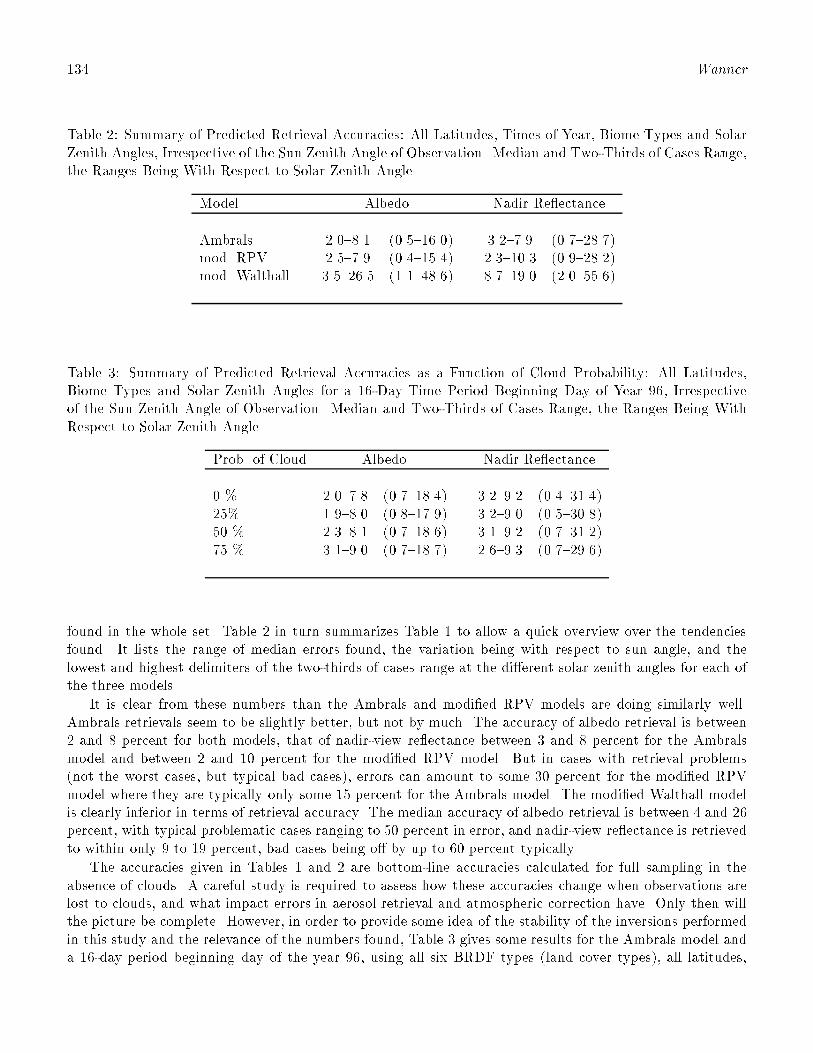
134 Wanner
Table 2: Summary of Predicted Retrieval Accuracies: All Latitudes, Times of Year, Biome Types and SolarZenith Angles, Irrespective of the Sun Zenith Angle of Observation. Median and Two-Thirds of Cases Range,the Ranges Being With Respect to Solar Zenith Angle.
Model Albedo Nadir Re ectance
Ambrals 2.0{8.1 (0.5{16.0) 3.2{7.9 (0.7{28.7)mod. RPV 2.5{7.9 (0.4{15.4) 2.3{10.3 (0.9{28.2)mod. Walthall 3.5{26.5 (1.1{48.6) 8.7{19.0 (2.0{55.6)
Table 3: Summary of Predicted Retrieval Accuracies as a Function of Cloud Probability: All Latitudes,Biome Types and Solar Zenith Angles for a 16-Day Time Period Beginning Day of Year 96, Irrespectiveof the Sun Zenith Angle of Observation. Median and Two-Thirds of Cases Range, the Ranges Being WithRespect to Solar Zenith Angle.
Prob. of Cloud Albedo Nadir Re ectance
0 % 2.0{7.8 (0.7{18.4) 3.2{9.2 (0.4{31.4)25% 1.9{8.0 (0.8{17.9) 3.2{9.0 (0.5{30.8)50 % 2.3{8.1 (0.7{18.6) 3.1{9.2 (0.7{31.2)75 % 3.1{9.0 (0.7{18.7) 2.6{9.3 (0.7{29.6)
found in the whole set. Table 2 in turn summarizes Table 1 to allow a quick overview over the tendenciesfound. It lists the range of median errors found, the variation being with respect to sun angle, and thelowest and highest delimiters of the two-thirds of cases range at the di�erent solar zenith angles for each ofthe three models.
It is clear from these numbers than the Ambrals and modi�ed RPV models are doing similarly well.Ambrals retrievals seem to be slightly better, but not by much. The accuracy of albedo retrieval is between2 and 8 percent for both models, that of nadir-view re ectance between 3 and 8 percent for the Ambralsmodel and between 2 and 10 percent for the modi�ed RPV model. But in cases with retrieval problems(not the worst cases, but typical bad cases), errors can amount to some 30 percent for the modi�ed RPVmodel where they are typically only some 15 percent for the Ambrals model. The modi�ed Walthall modelis clearly inferior in terms of retrieval accuracy. The median accuracy of albedo retrieval is between 4 and 26percent, with typical problematic cases ranging to 50 percent in error, and nadir-view re ectance is retrievedto within only 9 to 19 percent, bad cases being o� by up to 60 percent typically.
The accuracies given in Tables 1 and 2 are bottom-line accuracies calculated for full sampling in theabsence of clouds. A careful study is required to assess how these accuracies change when observations arelost to clouds, and what impact errors in aerosol retrieval and atmospheric correction have. Only then willthe picture be complete. However, in order to provide some idea of the stability of the inversions performedin this study and the relevance of the numbers found, Table 3 gives some results for the Ambrals model anda 16-day period beginning day of the year 96, using all six BRDF types (land cover types), all latitudes,
Retrieval Accuracies of BRDF and Albedo 135
and the red and the near-infrared bands. The probability of an observation to be lost due to cloudinesswas set in turn to 0, 25, 50 and 75 percent. Five realizations of each case were computed. In each of these,the number of observations varied, as did which observations were dropped, but the average number wasclose to three quarters, half, and one quarter of the full set. Observations were randomly dropped eventhough MISR observations are most likely to be dropped in multiples of 9 if they are dropped (since themultiangular observations are acquired simultaneously, which is not the case for MODIS). Inversions werepreformed on each case and the error ranges given in Table 3 computed.
Table 3 shows that neither albedo retrieval errors nor nadir re ectance retrieval errors change much evenwhen three quarters of all observations are dropped. The reason for this is that the most important factorin the inversions is not the number of observations but the range of angles they cover, which is mostly nota�ected by random dropouts of observations. The sensitivity of retrievals to various types of noise-like e�ectsin the observations will grow as the number of observations drops, but a study by Wanner et al. (1996) andLewis and Wanner (1997) has shown that noise sensitivity of Ambrals retrievals is rather good for combinedMODIS and MISR sampling, noise mostly not being ampli�ed into the BRDFs and albedos retrieved evenwith a loss of observations to clouds.
Consequently, it is safe to say that loss of observations to clouds are not a limiting factor with respectto the MODIS observations. And since at least two opportunities for a MISR observation occur in a 16-daytime period, in most cases actual MODIS/MISR sampling should be even better than obtained from thecomputed random loss. With some caution, the bottom-line accuracies derived in this study may be takenas a preliminary indication of expected product accuracy of the MODIS BRDF/Albedo Product. Table 1and Figure 6 give the full details.
6. Discussion and Conclusions
A word of caution is due with respect to the fact that this study was conducted in form of a model-to-modelcomparison. Since angular sampling has such a particular in uence in the values retrieved, it is importantto study retrieval accuracies using the actual sampling, not principal-plane sampling or cross-principal planesampling, even though those too may give an indication of what is achievable. In the absence of the actualinstruments, this makes necessary a study using simulation, such as this one, allowing to explore the fullrange of occurring situations. However, if an inverse model is not capable of producing good results, thereason may be sought with either the inverse model or the forward model. Particularly, deviations of theinverse from the forward model at large zenith angles, where theories involving projections are most likely tobe overly idealistic, may be caused by either model. It would be wrong to necessarily construct the inversionmodels in such a way that it absolutely follows the forward model. Furthermore, in this study the forwardmodel itself may have had some problems, for example due to the discreteness of the numerical schemeused. The BRDFs from DOM/RTCODE are rather similar across the biomes, either re ecting a similarityin the theories used for the di�erent biomes or re ecting a general similarity in natural BRDFs once bothshadowing and radiative transfer-type scattering are both taken into account at all levels.
However, it should also be pointed out that even after the MODIS and MISR instruments are operational,it will be very di�cult to replace these error estimates from simulation with values actually measured. Anyvalidation e�ort will necessarily be limited in the range of conditions covered, will have to deal with severeproblems of scaling between local observations and the size of the sensor footprints (e�ectively one kilometerfor the MODIS BRDF/Albedo Product), and be convolved with other uncertainties, stemming for examplefrom di�erences in the spectral response or calibration of the ground and the space instruments. Mostaccuracies considered in this study are in the range of a few percent, which to detect requires excellentaccuracy in the �eld.
In conclusion, it seems from this investigation that it is probable that BRDF and albedo will be retrievable
136 Wanner
with reasonable accuracy from MODIS and MISR observations using either the Ambrals or the modi�edRPV model. Typical errors will be below 10 percent. It is good that the MISR BRDF/Albedo Productwill be based on the modi�ed RPV model while the MODIS BRDF/Albedo Product will use the Ambralsmodel, as both models are capable of producing reliable results and using both models in di�erent productswill maximize the material generated from which conclusions can be drawn. The resulting BRDFs andalbedos can be assembled into databases that integrate knowledge over time, further minimizing the errorinvolved. These databases may then serve for a characterization of the radiative state of the Earth's surfacefor biophysical, climate and weather modeling.
Acknowledgements. Special thanks are due to Ranga Myneni for allowing generous use of his DOM/RTCODEBRDF modeling algorithm, without which this work would not have been possible. Baojin Zhang at BostonUniversity cooperated in early stages of this work. Thanks also to all members of the MODIS BRDF/Albedoteam for discussions, especially Philip Lewis, Alan Strahler, and Xiaowen Li; and to Petra Lucht. This workwas supported by NASA under NAS5-31369.
References
Barnsley, M. J., A. H. Strahler, K. P. Morris, and J.-P. Muller, Sampling the surface bidirectional re ectancedistribution function (BRDF): Evaluation of current and future satellite sensors, Remote Sens. Rev.
8, 271{311, 1994.
Deschamps, P. Y., F. M. Breon, M. Leroy, A. Podaire, A. Bricaud, J. C. Buriez, and G. Seze, The POLDERmission: Instrument characteristics and scienti�c objectives, IEEE Trans. Geosci. Remote Sens., 32,598{615, 1994.
Diner, D., C. J. Bruegge, J. V. Martonchik, G. W. Bothwell, E. D. Danielson, V. G. Ford, L. E. Hovland,K. L. Jones, and M. L. White, A multi-angle image spectroradiometer for terrestrial remote sensingwith the Earth Observing System, Int. J. Imag. Sys. Tech., 3, 92{107, 1991.
Diner, D., J. V. Martonchik, C. Borel, S. A. W. Gerstl, H. R. Gordon, R. Myneni, B. Pinty, and M. M. Ver-straete, MISR LEvel 2 Surface Retrieval Algorithm Theoretical Basis, NASA EOS-MISR Document,
JPL D-22401, Rev. B, 78 pp.1996.
Engelsen, O., B. Pinty, M. M. Verstraete, and J. V. Martonchik, Parametric bidirectional re ectance factormodels: evaluation, improvements and applications, Report, Joint Research Centre of the European
Commission, EU 16426,, 114 pp., 1996.
Hu, B., W. Wanner, X. Li, and A. Strahler, Validation of kernel-driven semiempirical BRDF models forapplication to MODIS-MISR data, Proc. Int. Geosci. Remote Sens. Symp. 96, 1669{1671, 1996.
Hu, B., W. Wanner, X. Li, and A. Strahler, Validation of kernel-driven semiempirical models for globalmodeling of bidirectional re ectance, to be submitted to Remote Sens. Env., 1997.
Lewis, P., and W. Wanner, Noise sensitivity of BRDF and albedo retrieval from the Earth ObservingSystem MODIS and MISR Sensors with respect to angular sampling, in preparation, 1997.
Leroy, M., J. L. Deuze, F. M. Breon, O. Hautecoeur, M. Herman, J. C. Buriez, D. Tanre, S. Bou�es, P.Chazette, and J.-L. Roujean, Retrieval of atmospheric properties and surface bidirectional re ectancesover land from POLDER/ADEOS, J. Geophys. Res., this issue, 1997.

Retrieval Accuracies of BRDF and Albedo 137
Li, X., and A. H. Strahler, Geometric-optical bidirectional re ectance modeling of the discrete crownvegetation canopy: e�ect of crown shape and mutual shadowing, IEEE Trans. Geosci. Remote Sens.,
30, 276{292, 1992.
Martonchik, J. V., Determination of aerosol optical depth and land surface directional re ectances usingmulti-angle imagery, J. Geophys. Res., in press, 1997.
Myneni, R. B., G. Asrar, and F. G. Hall, A three-dimensional radiative transfer method for optical remotesensing of vegetated land surfaces, Remote Sens. Env., 41, 105{121, 1992.
Nilson, T., and A. Kuusk, A re ectance model for the homogeneous plant canopy and its inversion, RemoteSens. Env., 27, 157{167, 1989.
Rahman, H., B. Pinty, and M. M. Verstraete, Coupled surface-atmosphere re ectance (CSAR) model, 2,Semiempirical surface model usable with NOAA advanced very high resolution radiometer data, J.Geophys. Res., 98, 20,791{20,801, 1993.
Roujean, J. L., M. Leroy, and P. Y. Deschamps, A bidirectional re ectance model of the earth's surface forthe correction of remote sensing data, J. Geophys. Res., 97, 20,455{20,468, 1992.
Ross, J. K., The Radiation Regime and Architecture of Plant Stands, 392 pp., Dr. W. Junk Publishers, TheHague, 1981.
Running, S. W., C. O. Justice, V. Salomonson, D. Hall, J. Barker, Y. J. Kaufman, A. H. Strahler, A. R.Huete, J.-P. Muller, V. Vanderbilt, Z. M. Wan, P. Teillet, and D. Carneggie, Terrestrial remote sensingscience and algorithms planned for EOS/MODIS, Int. J. Remote Sens., 15, 3587{3620, 1994.
Schaaf, C. B., and A. H. Strahler, Validation of bidirectional and hemispherical re ectances from ageometric-optical model using ASAS imagery and pyranometer measurements of a spruce forest, Re-mote Sens. Environ., 49, 138{144, 1994.
Schaaf, C. B., X. Li, and A. H. Strahler, Topographic e�ects on bidirectional and hemispherical re ectancescalculated with a geometric-optical canopy model, IEEE Trans. Geosci. Remote Sens., 32, 1186{1193,1994.
Strahler, A. H., C. B. Schaaf, J.-P. Muller, W. Wanner, M. J. Barnsley, R. d'Entremont, B. Hu, P. Lewis,X. Li, and E. V. Ruiz de Lope, MODIS BRDF/albedo product: Algorithm theoretical basis document,NASA EOS-MODIS Doc., version 4.0, 1996.
Walthall, C. L., J. M. Norman, J. M. Welles, G. Campbell, and B. L. Blad, Simple equation to approximatethe bidirectional re ectance from vegetation canopies and bare soil surfaces, Appl. Opt., 24, 383{387,1985.
Wanner, W., X. Li, and A. H. Strahler, On the derivation of kernels for kernel-driven models of bidirectionalre ectance, J. Geophys. Res., 100, 21077{21090, 1995.
Wanner, W., P. Lewis, and J.-L. Roujean, The in uence of directional sampling on bidirectional re ectanceand albedo retrieval using kernel-driven models, Proc. Int. Geosci. Remote Sens. Symp. 96, 1408{1410,1996.
Wanner, W., A. H. Strahler, B. Hu, X. Li, C. L. Barker Schaaf, P. Lewis, J.-P. Muller, and M. J. Barnsley,Global retrieval of bidirectional re ectance and albedo over land from EOS MODIS and MISR data:theory and algorithm, J. Geophys. Res., in press, 1997.

138 Lewis and Wanner
APPENDIX C:
NOISE SENSITIVITY OF BRDFANDALBEDORETRIEVAL FROM
THE EOS-MODIS AND MISR SENSORS WITH RESPECT TO AN-
GULAR SAMPLING (PAPER BY LEWIS AND WANNER)

Noise Sensitivity of BRDF and Albedo 139
PROGRESS REPORT (Nov. 96):Tables and �gures �nal; text will be completely revised
Noise Sensitivity of BRDF and Albedo Retrieval From theEarth Observing System MODIS and MISR Sensors With
Respect to Angular Sampling
Philip Lewis1 and Wolfgang Wanner2
1 Remote Sensing Unit, Dept. of Geography, University College London, London, UK2 Center for Remote Sensing and Dept. of Geography, Boston University, Boston, MA
Abstract
The sensitivity of the Ambrals semiempirical BRDF model to random noise in observed multiangular re- ectances is investigated. The mathematical properties of kernel-driven BRDF models allow to deriveanalytically so-called weights of determinations or noise in ation factors that quantify the expected noisefound in retrieved parameters like nadir-view re ectance or albedo at various solar zenith angles, or in theBRDF model parameters. The study is carried out using simulated angular sampling as is to be expectedfrom the MODIS and MISR instruments to be own on the EOS-AM platforms as a function of latitude,day of year and sampling period. A similar study is carried out for comparison using the modi�ed RPVBRDF model. Results show that for both models the retrieved parameters re ectance and albedo the noiseampli�cation factors are less than one (less noise present than was in the original data, i.e., the retrievals arestable with respect to random noise). The BRDF model parameters themselves, especially for the modi�edRPV model, are found to be more susceptible to noise. Di�erences in noise sensitivity between di�erentmodel variants and sampling scenarios are further explored. This study is relevant with respect to the re-liability to be expected from the planned operational BRDF/albedo products from the MODIS and MISRinstruments.
1. Introduction
Global space-based retrievals of the bidirectional re ectance distribution function (BRDF) and albedo overland will be possible in the near future using the Earth Observing System's (EOS) MODIS and MISR sensorsor the POLDER instrument. BRDF information is useful for normalizing satellite-acquired data sets andfor deriving key surface parameters, mainly atmospherically corrected albedo for use in climate studies.
Little work, however, has been done on the sensitivity of BRDF and albedo retrievals to angular samplingpatterns even though the impact of these on product accuracy is possibly substantial. With any instrument,the angular distribution of samples obtainable in a given time period will vary with geographic latitude andtime of year, and be also determined by instrument and orbit characteristics. Cloud masking will furtherreduce the set of available angular re ectances. In this paper we evaluate in a practical case the impact ofangular sampling e�ects on BRDF and albedo derivation.
Two e�ects mainly have an in uence on retrieval accuracy as a function of angular sampling:(1) Sensitivity to random noise. Analysis is carried out under the assumption that the RMSE found in

140 Lewis and Wanner
inverting a model against observations is due to random \noise-like" errors in the observed re ectances, duefor example to uctuations in surface properties, misregistration, atmospheric correction errors etc.(2) Mis�t sensitivity. Analysis is carried out under the assumption that the RMSE found in inversion isdue to an inherent partial inability of the model used to �t the observations even in the absence of \noise",and to infer completely from limited angular sampling the BRDF shape observed. Investigating this e�ectis important in view of the many assumptions that are commonly made in operationally feasible BRDFmodels.
In this paper, we focus on the noise sensitivity analysis alone, although the mis�t analysis is of equalimportance. We study the behavior of the semiempirical Ambrals BRDF model (Wanner et al., 1995, 1997)under conditions of sampling by MODIS and MISR, and how the semiempirical Rahman model (Rahmanet al., 1993) behaves under the same circumstances.
2. The Experiment
We here investigate sampling e�ects with respect to the MODIS BRDF/albedo product (Strahler et al.,1996; Wanner et al., 1997), using the sampling patterns and BRDF models characterizing it. The productis slated for production at a spatial resolution of one kilometer once every 16 days and in seven spectralbands from combined MODIS-AM and MISR data starting in 1998. The MODIS-AM sensor is an across-track imager with a swath width of 2330km, and a repeat rate shorter than 2 days (mostly shorter than1 day). MISR is an along-track imager with a swath width of 364km using four fore-, four aft- and onenadir-pointing camera. The two-look repeat rate is 16 days. In this time, each sensor produces a string ofobservations across the viewing hemisphere with rather constant relative azimuth and solar zenith angles.The two strings from the two instruments are nearly orthogonal; their respective azimuthal distance fromthe principal plane varies with latitude and time of year, as does the mean solar zenith of the observationsand the number of observations from MODIS.
The analysis was carried out for the Ambrals BRDF model that will be used in the production of theMODIS BRDF/albedo product. The kernel combinations used in that model are: RossThick-LiSparse,RossThin-LiSparse, RossThin-LiDense, and RossThick-LiDense (Wanner et al., 1995). These are capable ofmodelling a wide variety of volume and surface scattering behavior and which will be employed dependingon the scattering behavior observed.
Retrievals investigated are for nadir-view re ectance and directional-hemispherical (\black-sky") albedo.Both of these quantities are studied for retrievals at the mean sun angle of the observations (\interpolation")and for nadir sun zenith angle (\extrapolation", the amount of extrapolation depending on the sun angleof observations, which depends on the latitude and the time of year of the observations). Additionally,bihemispherical albedo (\white-sky albedo") is studied.
MODIS and MISR sampling was simulated using the Xsatview software (Barnsley et al., 1994). Theviewing and illumination geometries were constructed for 9 latitudes between 80 degrees south and 80 degreesnorth, and for 8 di�erent 16-day time periods throughout the year.
3. Noise Sensitivity of the Ambrals Model
3.1. Method
The behavior of kernel-driven linear models under the conditions of limited and varying angular samplingcan be studied analytically due to the mathematical form of these models. It is given by the the so-called\weights of determination", calculated using theory that originates with Gauss (Whittaker and Robinson,1960). Kernel-driven models give the re ectance R in form of a sum, R =
Pfiki, where fi are the model
Noise Sensitivity of BRDF and Albedo 141
parameters and ki are mathematical functions (\kernels") giving basic BRDF shapes depending only onsampling geometry.
The theory of least squares and related statistical analyses permit the derivation of unbiased estimatesof model parameters and linear combinations of model parameters (such as re ectances at given angles andalbedos for kernel-driven models). The techniques also directly provide estimates of the variance in thesequantities. An overview of the relevant tools for analysis is provided below, but it is worth �rst consideringthe nature of \error" in this context. The theory used here and that used in most model inversions in the�eld of BRDF modelling is based on the assumption that the model is suitable for modelling the re ectanceat some given location on the globe. Thus, if a model is \�tted" (in the sense of providing unbiased estimatesof the model parameters) to a set of sample observations, then the model should be capable of predictingthe re ectances (or derived quantities such as albedo-related terms) at viewing and illumination anglesother than those sampled. The theory assumes that any deviation from a perfect �t in an over-constrainedcase (number of samples larger than number of model parameters) is due to error in observation. Relatedstatistical theory tends to assume further that the variation in re ectance at each observation angle isnormally distributed and of equal variance over the re ectance function (if the variance of the re ectancevaries in some predictable way over the observation angles, this can be taken into account by weighting theobservations). The \error" in a model �t term which is minimized in \�tting" the model, the root meansquared error (RMSE), provides an estimate of this variance in observation. Such uctuations may indeedarise, due, for example, to uncertainty in atmospheric correction, registration or resampling. Some of these uctuations may cause normally distributed variation in the data, and others, such as poor speci�cation ofthe atmospheric intrinsic path radiance, may cause bias. The former is well-treated in the approach followedin this paper, and the latter may be taken into account in describing the additional expected error if anestimate of the bias is produced.
The key to understanding the behavior of kernel-driven linear models in the presence of random noise inthe observed data under the conditions of limited and varying angular sampling is the variation of the so-called \weights of determination" of the model parameters, derived re ectances and derived albedo measuresfound from model inversion. These weights allow an estimation of the expected error in the terms underconsideration, which can be expressed as (Whittaker and Robinson, 1960)
�u = e
s1
wu; (1)
where e is the estimate of standard error in the observed data (approximated by the RMSE in model �tting),and 1=wu is the weight of determination of term u under the sampling con�guration considered. The weightof determination is formed through
1
wu= [U ]T [M�1][U ]; (2)
where U is a vector composed of the weighting of the kernels in some linear combination of the kernelswhich results in the term u under consideration, and M�1 is the inverse matrix providing the solution ofthe least-squares inversion problem for the linear model.
For example, to obtain the weight of determination of the parameter f0= fiso of a kernel-driven model,
[U ]T = (1; 0; 0). The weight of determination of directional-hemispherical re ectance at solar zenith angle�s is formed from [U ]T = (1; k
1(�s); k2(�s)), where ki are the respective directional-hemispherical integrals
of the kernels used. The weight of determination of bihemispherical re ectanc is formed from [U ]T =
(1; k1; k
2), where two bars tand for the respective bihemispherical integral. The weight of determination
of the re ectance at some combination of viewing and illumination angles, (�v ; �s; �), is given by forming[U ]T = (1; k
1(�v ; �s; �); k2(�v ; �s; �)).
The weight of determination depends on the sampling scheme under consideration because M�1 dependson it. The weight of determination also depends on the number of samples, N , and contains the factor 1=
pN .

142 Lewis and Wanner
Increasing N decreases the expected error because the errors are assumed to be randomly distributed ateach observation angle. Thus, we can already begin to understand that factors such as cloud cover, whichwill reduce N from the maximum ideal number considered in this study to N 0, will tend to increase theexpected error even if the angular distribution of samples remains roughly the same. The increase in eachterm under consideration is given by
pN=N 0.
Note that this analysis is independent of any speci�c BRDF function.
3.2. Results for the Ambrals Model
In an extensive investigation, we have studied the sensitivity to random noise of the several Ambrals BRDFmodel variants listed above using sampling for a variety of combinations of the MODIS and MISR sensors,and for di�erent periods of data accumulation. Table 1 lists the weights of determination found for albedoand nadir view re ectance retrieval in interpolation and extrapolation for the di�erent Ambrals model kernelcombinations. Nearly all numbers are smaller than 1, indicating stability with respect to noise ampli�cationin deriving the respective quality.
Table 2 investigates median error ranges (the ranges re ecting variations with kernel combination used;the median being with respect to latitude and day of year) for di�erent sampling scenarios using MODISand MISR on the EOS-AM-1 platform and MODIS on the PM platform. The MISR BRDF/albedo product,which will be produced using the BRDF model by Rahman et al. (1993), will be based on a 9-day sam-pling period, whereas the MODIS BRDF/albedo product will be built from data acquired during 16-dayperiods. Since the RossThick and LiDense kernels are least independent in their angular characteristics,the RossThick-LiDense kernel combination is most susceptible to noise of all combinations. Therefore, welist results separately for using this combination and for using those kernels separately along with the otherkernel combinations. The lower part of the table lists relative changes in accuracy of the di�erent samplingschemes as measured against the combined MODIS and MISR 16-day sampling.
Table 2 shows that albedo and nadir-view re ectance may be stably retrieved both in interpolation andextrapolation of the solar zenith angle. This is also true for 9-day MISR sampling, showing that MISRangular sampling is very suitable for these retrievals. Using MODIS alone introduces susceptibility tonoise that is not desired. The MODIS-PM instrument is a partial, but not a full substitute for the MISRinstrument, the advantage of MODIS-PM being, however, that it will feature the same 7 land-designatedspectral bands as the MODIS-AM instrument, whereas MISR has only 4 bands.
Table 3 lists the worst-case ranges of the noise sensitivities found. \Worst-case" refers to the mostunfavorable choice of kernel combination; the numbers given are the range numbers that include two thirdsof the data for all latitudes and times of year.
Figure 1 shows the weights of determination found for the di�erent retrievals when using the RossThick-LiSparse model, chosen as a typical example. Curves represent di�erent days in the �rst half of the year.Panel (f) shows the error expected when extrapolating black-sky albedo in sun zenith angle for di�erentlatitudes and sampling in the �rst 16-day period of the year. One can see that extrapolation towards nadiris less problematic than extrapolation to large zenith angles for all latitudes, the beginning of the rise beingdetermined by the sun zenith angle at which the observations were made.
Overall, the noise sensitivity of the Ambrals BRDF model with respect to BRDF and albedo retrieval atthe sun zenith angles investigated is such that in the absence of clouds noise-like e�ects in the observationslead to a usually much smaller error in the derived quantities than was present in the re ectances. Underconditions where observations will be lost to clouds, the sensitivity will increase, but the noise in ationfactor will still be mostly smaller than unity.
Figure 2 shows the noise sensitivity of the model parameters themselves (note that the isotropic parameteris identical with nadir-view, nadir-sun re ectance, shown in Figure 1). They are more susceptible to noisethan the derived quantities due to possible tradeo�s between parameter values that do not a�ect, for example,
Noise Sensitivity of BRDF and Albedo 143
the value of albedo. This means that while albedo and re ectance retrievals are robust, interpretation ofthe model parameters themselves, desired with respect to correlating them with land cover types, is moreproblematic. See also the numbers in Tables 1, 2 and 3.
4. Noise Sensitivity of the modi�ed RPV model
The noise sensitivity of the RPV BRDF model by Rahman et al. (1993) as modi�ed by Martonchik (Engelsenet al., 1996) was also investigated for comparison and in order to reveal whether the properties found arerelated to the Ambrals model in particular or whether they might pertain to 3-parameter models in general.
The modi�ed RPV model is not fully linear, making the analytical investigation of noise sensitivity alongthe lines of the Ambrals BRDF model impossible. However, an equivalent weight of determination may beconstructed from the RMSE and the variation found in the derived quantity, albedo or re ectance. This wasdone by computing 250 realizations of noisy data for each of 5 magnitudes of noise up to 5 percent absoluteof the re ectance (keeping the resulting re ectance is non-negative).
Due to the nonlinear nature of the modi�ed RPV model, the analysis will also depend on land covertype and wave band. The analysis was carried out for the red and the near-infrared using four di�erent datasets measured by Kimes (1983) and Kimes et al. (1985, 1986), namely BRDF observations of corn, a plowed�eld, a hardwood forest and a grass lawn. These represent four types of BRDFs, a broadleaf crop, a barrenscene, a forested scene, and a grass-like land cover.
Table 4 gives ranges of the inferred equivalent weights of determination. Numbers are similar to thosefound for the Ambrals BRDF model, showing that both models do a good job in the stability of the retrievalswith respect to random noise.
Figure 3 shows red and near-infrared weights of determinations as a function of latitude for a 16-dayperiod beginning the �rst day of the year for the four land cover types used (solid and dotted lines). Alsogiven is the result for the RossThick-LiSparse Ambrals model kernel combination (dashed line), showingthat where one model has increased sensitivity to noise the other one does, too.
Figure 2 shows the sensitivity of the three modi�ed RPV model parameters. The second and thirdparameters, the two describing BRDF shape, are extremely susceptible to noise. This does not translate tonoisy retrievals of re ectance and albedo, but will make very di�cult using and interpreting them directly.The cause of this sensitivity is probably internal redundancy in the way these parameters a�ect overall BRDFshape, perhaps caused by the hotspot term the model contains that allows tradeo�s between parametersunder limited angular sampling. However, since the model retrieves albedo and re ectance very well, thisdoes not constitute a major problem in terms of physical quantities to be retrieved.
A more detailed investigation is under way.
5. Conclusions
Retrievals of BRDF and albedo using the Ambrals BRDF model is stable against random noise-like variationsin the re ectances used that may be due for example to uctuations in surface properties, misregistration,atmospheric correction errors etc. This holds both for retrieval of BRDF and albedo at the mean sunangle of observation and for extrapolation of the retrieval to a nadir sun zenith angle. Where the AmbralsBRDF model shows increased susceptibility to noise, the modi�ed RPV model does, as well, indicatingthat the source of the problem lies in the geometric distribution of angular samples available, not with themodel. Generally, the modi�ed RPV model is as capable of retrieving BRDF and albedo from MODISand MISR sampling as the Ambrals BRDF model. The respective model parameters themselves are morenoisy than the derived quantities BRDF and albedo for both models, but much more so for two of the threeparameters of the modi�ed RPV model. In terms of using di�erent instruments for sampling, a combination

144 Lewis and Wanner
of MODIS and MISR leads to excellent retrievals in terms of noise sensitivity. Using MISR only is alsofeasible. Using MODIS alone may represent a problem due to the less favorable angular sampling propertiesof this instrument.
Acknowledgments
We thank Mike Barnsley and Kevin Morris for providing the Xsatview software for orbital modeling, withoutwhich this work would have been impossible. This work was partly supported by NASA under NAS5-31369.
References
Barnsley, M. J., A. H. Strahler, K. P. Morris, and J.-P. Muller, Sampling the surface bidirectional re ectancedistribution function (BRDF): Evaluation of current and future satellite sensors, Remote Sens. Rev.
8, 271{311, 1994.
Engelsen, O., B. Pinty, M. M. Verstraete, and J. V. Martonchik, Parametric bidirectional re ectance factormodels: evaluation, improvements and applications, Report, Joint Research Centre of the European
Commission, EU 16426,, 114 pp., 1996.
Kimes, D. S., Dynamics of directional re ectance factor distribution for vegetation canopies, Appl. Opt.,22(9), 1364{1372, 1983.
Kimes, D. S., W. W. Newcomb, C. J. Tucker, I. S. Zonneveldt, W. van Wijngaarden, J. de Leeuw, andG. F. Epema, Directional re ectance factor distributions for cover types of Northern Africa, RemoteSens. Env., 18, 1{19, 1985.
Kimes, D. S., W. W. Newcomb, R. F. Nelson, and J. B. Schutt, Directional re ectance distributions of ahardwood and a pine forest canopy, IEEE Trans. Geosci. Remote Sens., 24, 281{293, 1986.
Rahman, H., B. Pinty, and M. M. Verstraete, Coupled surface-atmosphere re ectance (CSAR) model, 2,Semiempirical surface model usable with NOAA advanced very high resolution radiometer data, J.Geophys. Res., 98, 20,791{20,801, 1993.
Strahler, W. Wanner, A. H., C. B. Schaaf, J.-P. Muller, M. J. Barnsley, R. d'Entremont, B. Hu, P. Lewis,X. Li, and E. V. Ruiz de Lope, MODIS BRDF/albedo product: Algorithm theoretical basis document,NASA EOS-MODIS Doc., version 4.0, 1996.
Wanner, W., X. Li, and A. H. Strahler, On the derivation of kernels for kernel-driven models of bidirectionalre ectance, J. Geophys. Res., 100, 21077{21090, 1995.
Wanner, W., A. H. Strahler, B. Hu, X. Li, C. L. Barker Schaaf, P. Lewis, J.-P. Muller, and M. J. Barnsley,Global retrieval of bidirectional re ectance and albedo over land from EOS MODIS and MISR data:theory and algorithm, J. Geophys. Res., in press, 1997.
Whittaker, E., and G. Robinson, The Calculus of Observations, Blachie and Son, Glasgow, 397 pp., 1960.

Noise Sensitivity of BRDF and Albedo 145
Table 1: Weights of Determination for MODIS-AM/MISR 16-Day Sampling: Typical Small,
Median and Large Error for Different Kernel-Driven BRDF Models
MODIS{AM+MISR16-Day Sampling kernel 1 kernel 2 low median high low median high
Nadir-View Re ectance Black-Sky Albedo
Interpolation RossThin 0.17 0.21 0.24 0.14 0.17 0.19�s = h�si RossThick 0.17 0.18 0.21 0.12 0.16 0.17
LiSparse 0.14 0.19 0.25 0.13 0.17 0.18LiDense 0.15 0.18 0.19 0.12 0.16 0.18RossThin LiSparse 0.18 0.23 0.27 0.14 0.17 0.19RossThin LiDense 0.17 0.22 0.24 0.15 0.18 0.20RossThick LiSparse 0.18 0.23 0.28 0.13 0.17 0.18RossThick LiDense 0.17 0.19 0.22 0.13 0.16 0.18
Extrapolation RossThin 0.19 0.23 0.25 0.15 0.17 0.19�s = 0 RossThick 0.16 0.17 0.19 0.16 0.18 0.21
LiSparse 0.38 0.44 0.53 0.16 0.18 0.28LiDense 0.48 0.62 0.71 0.18 0.21 0.28RossThin LiSparse 0.38 0.45 0.55 0.16 0.18 0.33RossThin LiDense 0.73 0.93 1.08 0.19 0.28 0.49RossThick LiSparse 0.40 0.46 0.55 0.17 0.21 0.36RossThick LiDense 1.03 1.35 1.71 0.39 0.52 0.63
White-Sky Albedo
Global,R�sd�s RossThin 0.14 0.31 0.64
RossThick 0.14 0.18 0.34LiSparse 0.18 0.30 0.43LiDense 0.13 0.17 0.23RossThin LiSparse 0.19 0.36 0.64RossThin LiDense 0.21 0.42 0.82RossThick LiSparse 0.19 0.34 0.58RossThick LiDense 0.16 0.36 1.05
Parameter fvol Parameter fgeo
Parameters RossThin 0.04 0.14 0.25RossThick 0.32 0.89 1.74LiSparse 0.18 0.27 0.31LiDense 0.34 0.46 0.57RossThin LiSparse 0.05 0.15 0.30 0.19 0.28 0.36RossThin LiDense 0.07 0.17 0.29 0.45 0.60 0.69RossThick LiSparse 0.33 0.89 1.76 0.20 0.27 0.31RossThick LiDense 0.62 1.86 4.14 0.60 0.86 1.34
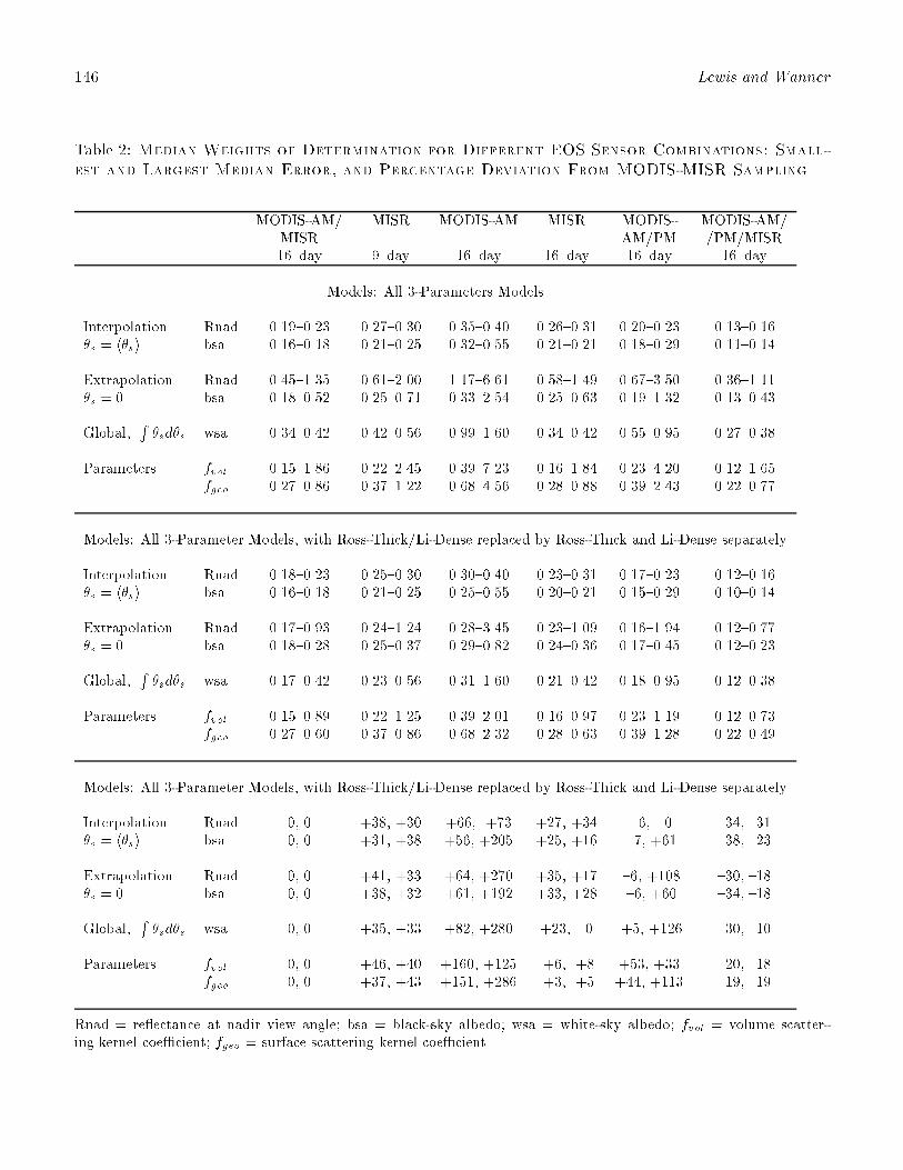
146 Lewis and Wanner
Table 2: Median Weights of Determination for Different EOS Sensor Combinations: Small-
est and Largest Median Error, and Percentage Deviation From MODIS-MISR Sampling
MODIS-AM/ MISR MODIS-AM MISR MODIS- MODIS-AM/MISR AM/PM /PM/MISR16{day 9{day 16{day 16{day 16{day 16{day
Models: All 3-Parameters Models
Interpolation Rnad 0.19{0.23 0.27{0.30 0.35{0.40 0.26{0.31 0.20{0.23 0.13{0.16�s = h�si bsa 0.16{0.18 0.21{0.25 0.32{0.55 0.21{0.21 0.18{0.29 0.11{0.14
Extrapolation Rnad 0.45{1.35 0.61{2.00 1.17{6.61 0.58{1.49 0.67{3.50 0.36{1.11�s = 0 bsa 0.18{0.52 0.25{0.71 0.33{2.54 0.25{0.63 0.19{1.32 0.13{0.43
Global,R�sd�s wsa 0.34{0.42 0.42{0.56 0.99{1.60 0.34{0.42 0.55{0.95 0.27{0.38
Parameters fvol 0.15{1.86 0.22{2.45 0.39{7.23 0.16{1.84 0.23{4.20 0.12{1.65fgeo 0.27{0.86 0.37{1.22 0.68{4.56 0.28{0.88 0.39{2.43 0.22{0.77
Models: All 3-Parameter Models, with Ross-Thick/Li-Dense replaced by Ross-Thick and Li-Dense separately
Interpolation Rnad 0.18{0.23 0.25{0.30 0.30{0.40 0.23{0.31 0.17{0.23 0.12{0.16�s = h�si bsa 0.16{0.18 0.21{0.25 0.25{0.55 0.20{0.21 0.15{0.29 0.10{0.14
Extrapolation Rnad 0.17{0.93 0.24{1.24 0.28{3.45 0.23{1.09 0.16{1.94 0.12{0.77�s = 0 bsa 0.18{0.28 0.25{0.37 0.29{0.82 0.24{0.36 0.17{0.45 0.12{0.23
Global,R�sd�s wsa 0.17{0.42 0.23{0.56 0.31{1.60 0.21{0.42 0.18{0.95 0.12{0.38
Parameters fvol 0.15{0.89 0.22{1.25 0.39{2.01 0.16{0.97 0.23{1.19 0.12{0.73fgeo 0.27{0.60 0.37{0.86 0.68{2.32 0.28{0.63 0.39{1.28 0.22{0.49
Models: All 3-Parameter Models, with Ross-Thick/Li-Dense replaced by Ross-Thick and Li-Dense separately
Interpolation Rnad 0, 0 +38, +30 +66, +73 +27, +34 {6, 0 {34, {31�s = h�si bsa 0, 0 +31, +38 +56, +205 +25, +16 {7, +61 {38, {23
Extrapolation Rnad 0, 0 +41, +33 +64, +270 +35, +17 {6, +108 {30, {18�s = 0 bsa 0, 0 +38, +32 +61, +192 +33, +28 {6, +60 {34, {18
Global,R�sd�s wsa 0, 0 +35, +33 +82, +280 +23, 0 +5, +126 {30, {10
Parameters fvol 0, 0 +46, +40 +160, +125 +6, +8 +53, +33 {20, {18fgeo 0, 0 +37, +43 +151, +286 +3, +5 +44, +113 {19, {19
Rnad = re ectance at nadir view angle; bsa = black-sky albedo; wsa = white-sky albedo; fvol = volume scatter-ing kernel coe�cient; fgeo = surface scattering kernel coe�cient.
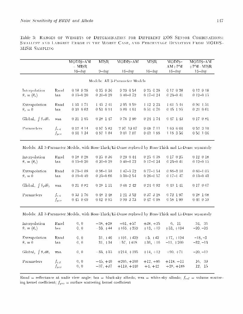
Noise Sensitivity of BRDF and Albedo 147
Table 3: Ranges of Weights of Determination for Different EOS Sensor Combinations:
Smallest and Largest Error in the Worst Case, and Percentage Deviation From MODIS-
MISR Sampling
MODIS{AM MISR MODIS{AM MISR MODIS{ MODIS{AM+ MISR AM+PM +PM+MISR16{day 9{day 16{day 16{day 16{day 16{day
Models: All 3-Parameter Models
Interpolation Rnad 0.18{0.28 0.25{0.36 0.29{0.54 0.25{0.38 0.17{0.28 0.12{0.18�s = h�si bsa 0.15{0.20 0.20{0.29 0.40{0.72 0.17{0.24 0.23{0.41 0.12{0.15
Extrapolation Rnad 1.03{1.71 1.45{2.41 2.95{9.59 1.12{2.23 1.61{5.44 0.90{1.51�s = 0 bsa 0.39{0.63 0.53{0.94 0.80{4.01 0.51{0.76 0.45{1.95 0.29{0.61
Global,R�sd�s wsa 0.21{1.05 0.28{1.47 0.76{2.90 0.24{1.74 0.47{1.43 0.17{0.81
Parameters fvol 0.62{4.14 0.87{5.83 2.97{13.07 0.68{7.11 1.63{6.60 0.52{3.10fgeo 0.60{1.34 0.87{1.84 2.01{7.07 0.62{1.88 1.18{3.56 0.56{1.06
Models: All 3-Parameter Models, with Ross-Thick/Li-Dense replaced by Ross-Thick and Li-Dense separately
Interpolation Rnad 0.18{0.28 0.25{0.36 0.29{0.44 0.25{0.38 0.17{0.25 0.12{0.18�s = h�si bsa 0.15{0.20 0.20{0.29 0.40{0.72 0.17{0.24 0.23{0.41 0.12{0.15
Extrapolation Rnad 0.73{1.08 0.96{1.58 1.47{5.72 0.77{1.54 0.86{3.18 0.60{1.05�s = 0 bsa 0.19{0.49 0.25{0.66 0.30{2.54 0.26{0.57 0.17{1.47 0.13{0.43
Global,R�sd�s wsa 0.21{0.82 0.28{1.11 0.66{2.42 0.24{0.92 0.40{1.41 0.17{0.67
Parameters fvol 0.33{1.76 0.48{2.48 1.21{3.52 0.37{3.28 0.72{1.97 0.28{1.08fgeo 0.45{0.69 0.62{0.95 0.99{3.73 0.47{0.98 0.58{1.99 0.40{0.59
Models: All 3-Parameter Models, with Ross-Thick/Li-Dense replaced by Ross-Thick and Li-Dense separately
Interpolation Rnad 0, 0 +38, +28 +61, +57 +38, +35 {6, {11 {34, {36�s = h�si bsa 0, 0 +33, +44 +166, +259 +13, +19 +53, +104 {20, {26
Extrapolation Rnad 0, 0 +31, +46 +101, +429 +5, +42 +17, +194 {18, {3�s = 0 bsa 0, 0 +31, +34 +57, +418 +36, +16 {11, +200 {32, {13
Global,R�sd�s wsa 0, 0 +33, +35 +214, +195 +14, +12 +90, +71 {20, {19
Parameters fvol 0, 0 +45, +40 +266, +100 +12, +86 +118, +11 {16, {39fgeo 0, 0 +37, +37 +119, +440 +4, +42 +28, +188 {12, {15
Rnad = re ectance at nadir view angle; bsa = black-sky albedo; wsa = white-sky albedo; fvol = volume scatter-ing kernel coe�cient; fgeo = surface scattering kernel coe�cient.
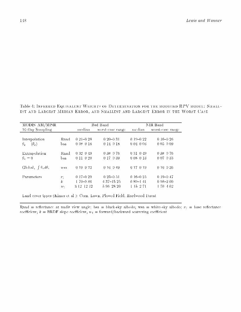
148 Lewis and Wanner
Table 4: Inferred Equivalent Weights of Determination for the modified RPV model: Small-
est and Largest Median Error, and Smallest and Largest Error in the Worst Case
MODIS{AM/MISR Red Band NIR Band16-Day Sampling median worst-case range median worst-case range
Interpolation Rnad 0.21{0.28 0.20{0.31 0.19{0.22 0.16{0.26�s = h�si bsa 0.08{0.16 0.14{0.18 0.04{0.06 0.05{0.09
Extrapolation Rnad 0.32{0.49 0.38{0.76 0.31{0.49 0.38{0.76�s = 0 bsa 0.11{0.20 0.17{0.39 0.08{0.13 0.07{0.33
Global,R�sd�s wsa 0.19{0.23 0.16{0.49 0.17{0.19 0.10{0.36
Parameters r0 0.17{0.29 0.23{0.51 0.16{0.25 0.19{0.47k 1.70{9.86 4.37{15.25 0.89{1.41 0.98{2.00w1 3.12{12.12 5.96{28.20 1.15{2.71 1.70{4.02
Land cover types (Kimes et al.): Corn, Lawn, Plowed Field, Hardwood Forest
Rnad = re ectance at nadir view angle; bsa = black-sky albedo; wsa = white-sky albedo; r0 = base re ectancecoe�cient; k = BRDF slope coe�cient; w1 = forward/backward scattering coe�cient.
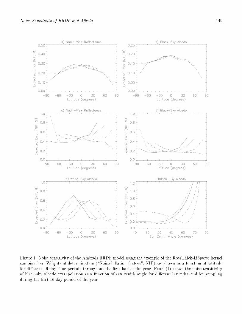
Noise Sensitivity of BRDF and Albedo 149
Figure 1: Noise sensitivity of the Ambrals BRDF model using the example of the RossThick-LiSparse kernelcombination. Weights of determination (\Noise in ation factors", NIF) are shown as a function of latitudefor di�erent 16-day time periods throughout the �rst half of the year. Panel (f) shows the noise sensitivityof black-sky albedo extrapolation as a function of sun zenith angle for di�erent latitudes and for samplingduring the �rst 16-day period of the year.
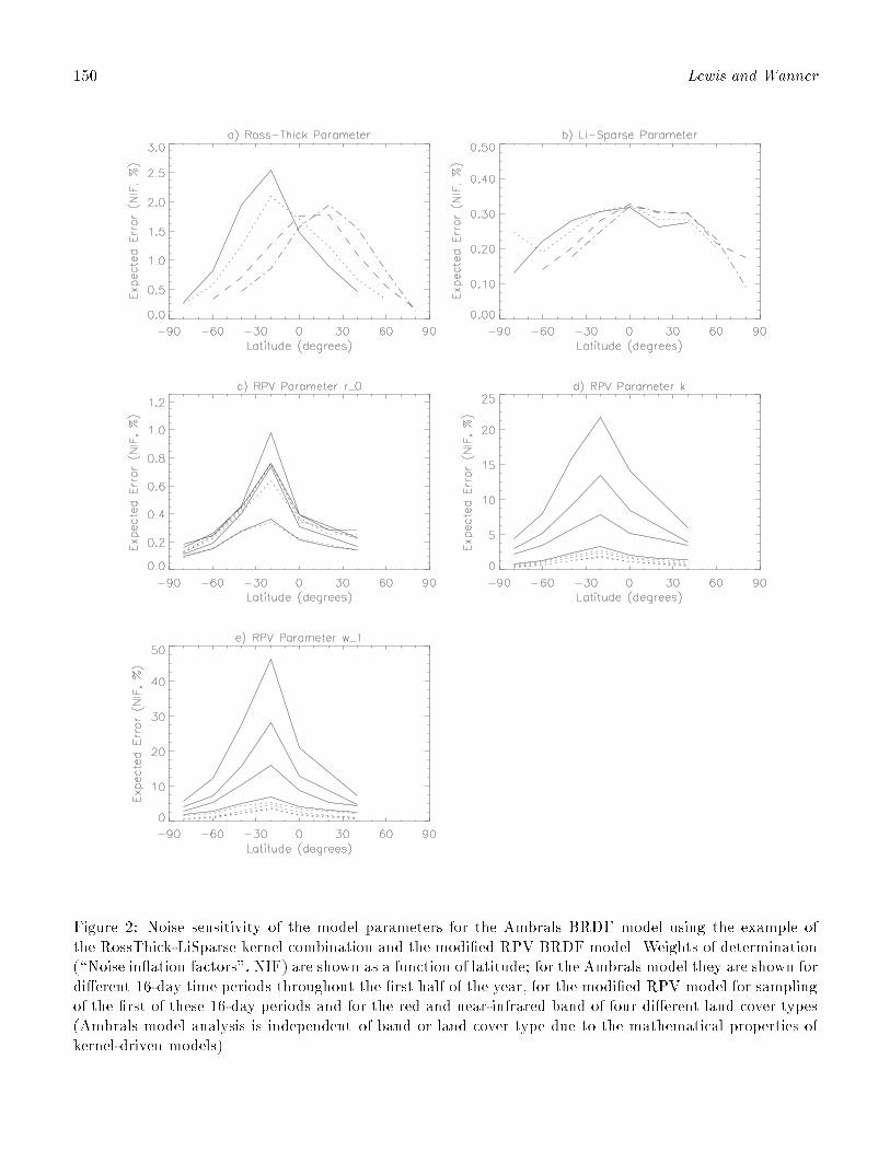
150 Lewis and Wanner
Figure 2: Noise sensitivity of the model parameters for the Ambrals BRDF model using the example ofthe RossThick-LiSparse kernel combination and the modi�ed RPV BRDF model. Weights of determination(\Noise in ation factors", NIF) are shown as a function of latitude; for the Ambrals model they are shown fordi�erent 16-day time periods throughout the �rst half of the year, for the modi�ed RPV model for samplingof the �rst of these 16-day periods and for the red and near-infrared band of four di�erent land cover types(Ambrals model analysis is independent of band or land cover type due to the mathematical properties ofkernel-driven models).

Noise Sensitivity of BRDF and Albedo 151
Figure 3: Noise sensitivity of the modi�ed RPV BRDF model. Inferred equivalent weights of determination(\Noise in ation factors", NIF) are shown as a function of latitude for the �rst 16-day period of the year andfor the red and near-infrared band of four di�erent land cover types (solid and dotted lines). Also shown isare the weights of determination for the Ambrals BRDF models using the example of the RossThick-LiSparsekernel combination (dashed lines).

152 Hu, Wanner and Strahler
APPENDIX D:
THE SENSITIVITY OF ATMOSPHERIC CORRECTION OF RE-
FLECTANCES TO THE SURFACE BRDF (PAPER BY HU, WAN-
NER AND STRAHLER)
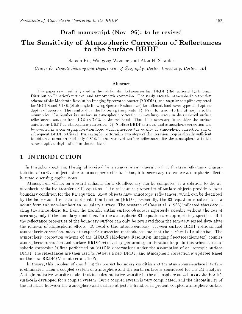
Sensitivity of Atmospheric Correction to the BRDF 153
Draft manuscript (Nov. 96): to be revised
The Sensitivity of Atmospheric Correction of Re ectancesto the Surface BRDF
Baoxin Hu, Wolfgang Wanner, and Alan H. Strahler
Center for Remote Sensing and Department of Geography, Boston University, Boston, MA
Abstract
This paper systematically studies the relationship between surface BRDF (Bidirectional Re ectanceDistribution Function) retrieval and atmospheric correction. The study uses the atmospheric correctionscheme of the Moderate Resolution Imaging Spectroradiometer (MODIS), and angular sampling expectedfor MODIS and MISR (Multiangle Imaging Spectro-Radiometer) for di�erent land cover types and opticaldepths of aerosols. The results show the following two points. 1). Even for a non-turbid atmosphere, theassumption of a Lambertian surface in atmospheric correction causes large errors in the retrieved surfacere ectances, such as from 1:7% to 7:6% in the red band. Thus, it is necessary to consider the surfaceanisotropic BRDF in atmospheric correction. 2). Surface BRDF retrieval and atmospheric correction canbe coupled in a converging iteration loop, which improves the quality of atmospheric correction and ofsubsequent BRDF retrieval. For example, performing two steps of the iteration loop is already su�cientto obtain a mean error of only 0:89% in the retrieved surface re ectances for the atmosphere with theaerosol optical depth of 0:4 in the red band.
1. INTRODUCTION
In the solar spectrum, the signal received by a remote sensor doesn't re ect the true re ectance charac-teristics of surface objects, due to atmospheric e�ects. Thus, it is necessary to remove atmospheric e�ectsin remote sensing applications.
Atmospheric e�ects on upward radiance for a cloudless sky can be computed as a solution to the at-mospheric radiative transfer (RT) equation. The re ectance properties of surface objects provide a lowerboundary condition for the RT equation. Most objects have anisotropic re ectances, which can be describedby the bidirectional re ectance distribution function (BRDF). Generally, the RT equation is solved with anonuniform and non-Lambertian boundary surface. The research of Case et al. (1953) indicated that decou-pling the atmospheric RT from the transfer within surface objects is rigorously possible without the loss ofaccuracy, only if the boundary conditions for the atmospheric RT equation are appropriately speci�ed. Butthe re ectance properties of the boundary surface can only be retrieved from the remotely sensed data afterthe removal of atmospheric e�ects. To resolve this interdependency between surface BRDF retrieval andatmospheric correction, most atmospheric correction methods assume that the surface is Lambertian. Theatmospheric correction scheme of the MODIS (Moderate Resolution Imaging Spectroradiometer) couplesatmospheric correction and surface BRDF retrieval by performing an iteration loop. In this scheme, atmo-spheric correction is �rst performed on MODIS observations under the assumption of an isotropic surfaceBRDF; the re ectances are then used to retrieve a new BRDF, and atmospheric correction is updated basedon the new BRDF (Vermote et al., 1995).
In theory, this problem of specifying the correct boundary conditions at the atmosphere-surface interfaceis eliminated when a coupled system of atmosphere and the earth surface is considered for the RT analysis.A single radiative transfer model that includes radiative transfer in the atmosphere as well as at the Earth'ssurface is developed for a coupled system. But a coupled system is very complicated, and the discontinuity ofthe interface between the atmosphere and surface objects is handled in present coupled atmosphere-surface
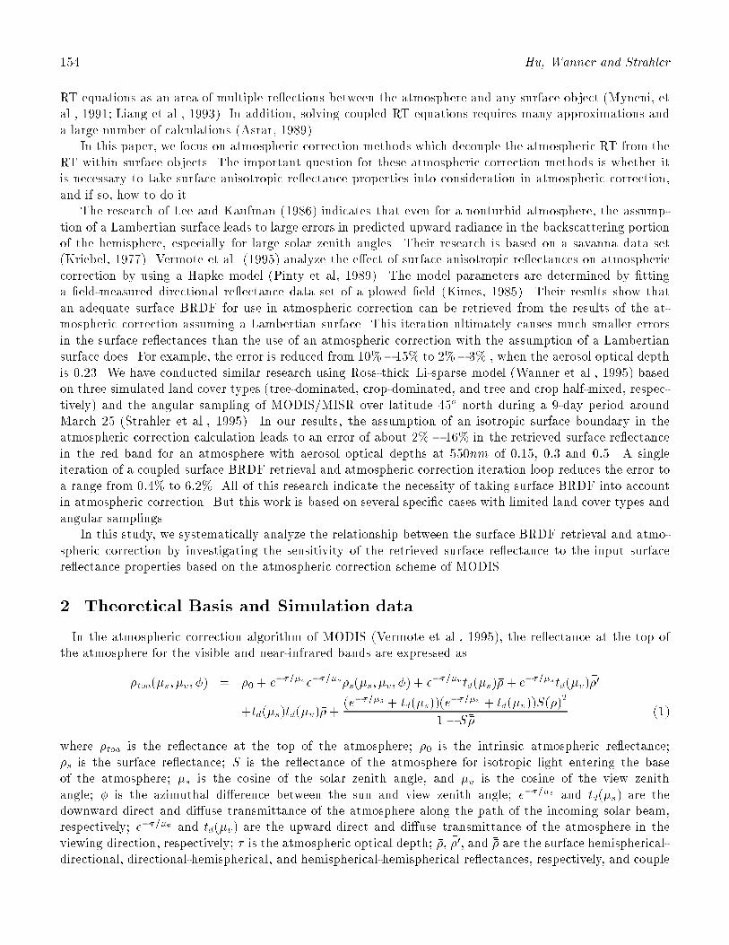
154 Hu, Wanner and Strahler
RT equations as an area of multiple re ections between the atmosphere and any surface object (Myneni, etal., 1991; Liang et al., 1993). In addition, solving coupled RT equations requires many approximations anda large number of calculations (Asrar, 1989).
In this paper, we focus on atmospheric correction methods which decouple the atmospheric RT from theRT within surface objects. The important question for these atmospheric correction methods is whether itis necessary to take surface anisotropic re ectance properties into consideration in atmospheric correction,and if so, how to do it.
The research of Lee and Kaufman (1986) indicates that even for a nonturbid atmosphere, the assump-tion of a Lambertian surface leads to large errors in predicted upward radiance in the backscattering portionof the hemisphere, especially for large solar zenith angles. Their research is based on a savanna data set(Kriebel, 1977). Vermote et al. (1995) analyze the e�ect of surface anisotropic re ectances on atmosphericcorrection by using a Hapke model (Pinty et al, 1989). The model parameters are determined by �ttinga �eld-measured directional re ectance data set of a plowed �eld (Kimes, 1985). Their results show thatan adequate surface BRDF for use in atmospheric correction can be retrieved from the results of the at-mospheric correction assuming a Lambertian surface. This iteration ultimately causes much smaller errorsin the surface re ectances than the use of an atmospheric correction with the assumption of a Lambertiansurface does. For example, the error is reduced from 10%�15% to 2%�3% , when the aerosol optical depthis 0:23. We have conducted similar research using Ross-thick{Li-sparse model (Wanner et al., 1995) basedon three simulated land cover types (tree-dominated, crop-dominated, and tree and crop half-mixed, respec-tively) and the angular sampling of MODIS/MISR over latitude 45o north during a 9-day period aroundMarch 25 (Strahler et al., 1995). In our results, the assumption of an isotropic surface boundary in theatmospheric correction calculation leads to an error of about 2%� 16% in the retrieved surface re ectancein the red band for an atmosphere with aerosol optical depths at 550nm of 0:15, 0:3 and 0:5. A singleiteration of a coupled surface BRDF retrieval and atmospheric correction iteration loop reduces the error toa range from 0:4% to 6:2%. All of this research indicate the necessity of taking surface BRDF into accountin atmospheric correction. But this work is based on several speci�c cases with limited land cover types andangular samplings.
In this study, we systematically analyze the relationship between the surface BRDF retrieval and atmo-spheric correction by investigating the sensitivity of the retrieved surface re ectance to the input surfacere ectance properties based on the atmospheric correction scheme of MODIS.
2. Theoretical Basis and Simulation data
In the atmospheric correction algorithm of MODIS (Vermote et al., 1995), the re ectance at the top ofthe atmosphere for the visible and near-infrared bands are expressed as
�toa(�s; �v; �) = �0+ e
��=�ve��=�s�s(�s; �v; �) + e
��=�vtd(�s)��+ e��=�std(�v)��0
+td(�s)td(�v)���+(e��=�s + td(�s))(e
��=�v + td(�v))S(���)2
1� S���(1)
where �toa is the re ectance at the top of the atmosphere; �0is the intrinsic atmospheric re ectance;
�s is the surface re ectance; S is the re ectance of the atmosphere for isotropic light entering the baseof the atmosphere; �s is the cosine of the solar zenith angle, and �v is the cosine of the view zenithangle; � is the azimuthal di�erence between the sun and view zenith angle; e��=�s and td(�s) are thedownward direct and di�use transmittance of the atmosphere along the path of the incoming solar beam,respectively; e��=�v and td(�v) are the upward direct and di�use transmittance of the atmosphere in theviewing direction, respectively; � is the atmospheric optical depth; ��, ��0, and ��� are the surface hemispherical-directional, directional-hemispherical, and hemispherical-hemispherical re ectances, respectively, and couple
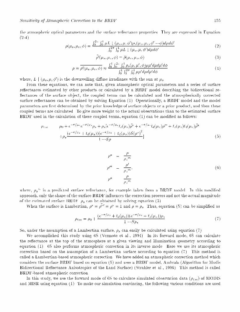
Sensitivity of Atmospheric Correction to the BRDF 155
the atmospheric optical parameters and the surface re ectance properties. They are expressed in Equation(2-4).
��(�s; �v; �) =
R2�0
R1
0�L # (�s; �; �0)�s(�s; �v; �0 � �)d�d�0R
2�0
R1
0�L # (�s; �; �0)d�d�0
(2)
��0(�s; �v; �) = ��(�v; �s; �) (3)
��� = ��0(�s; �v; �) �R1
0
R2�0
R1
0�s(�; �
0; �)��0d�d�0d�R1
0
R2�0
R1
0��0d�d�0d�
(4)
where, L # (�s; �; �0) is the downwelling di�use irradiance with the sun at �s.From these equations, we can note that, given atmospheric optical parameters and a series of surface
re ectances estimated by other products or calculated by a BRDF model describing the bidirectional re- ectances of the surface object, the coupled terms can be calculated and the atmospherically correctedsurface re ectances can be obtained by solving Equation (1). Operationally, a BRDF model and the modelparameters are �rst determined by the prior knowledge of surface objects or a prior product, and then thesecoupled terms are calculated. To give more weight to the actual observations than to the estimated surfaceBRDF used in the calculation of these coupled terms, equation (1) can be modi�ed as follows:
�toa = �0+ e
��=�ve��=�s�s + �s[e
��=�vtd(�s) ��� + e��=�std(�v) ��0
� + td(�s)td(�v) ����
+�s(e��=�s + td(�s))(e��=�v + td(�v))S( ����)
2
1� S���] (5)
��� =��
�sm
��0� =��0
�sm; (6)
���� =���
�sm
where, �sm is a predicted surface re ectance, for example taken from a BRDF model. In this modi�edapproach, only the shape of the surface BRDF in uences the correction process and not the actual magnitudeof the estimated surface BRDF. �s can be obtained by solving equation (5).
When the surface is Lambertian, ��� = ���0 = ���� = 1 and ��� = �s. Thus, equation (5) can be simpli�ed as
�toa = �0+(e��=�s + td(�s))(e
��=�v + td(�v))�s1� S�s
(7)
So, under the assumption of a Lambertian surface, �s can easily be calculated using equation (7).We accomplished this study using 6S (Vermote et al., 1994). In its forward mode, 6S can calculate
the re ectance at the top of the atmosphere at a given viewing and illumination geometry according toequation (1). 6S also performs atmospheric correction in its inverse mode. Here we use its atmosphericcorrection based on the assumption of a Lambertian surface according to equation (7). This method iscalled a Lambertian-based atmospheric correction. We have added an atmospheric correction method whichconsiders the surface BRDF based on equation (5) and uses a BRDF model, Ambrals (Algorithm for ModisBidirectional Re ectance Anisotropics of the Land Surface) (Strahler et al., 1996). This method is calledBRDF-based atmospheric correction.
In this study, we use the forward mode of 6S to calculate simulated observation data (�toa) of MODISand MISR using equation (1). To make our simulation convincing, the following various conditions are used
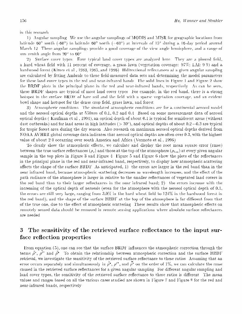
156 Hu, Wanner and Strahler
in this research.1). Angular sampling. We use the angular samplings of MODIS and MISR for geographic locations from
latitude 60o south (-60o) to latitude 60o north (+60o) at intervals of 15o during a 16-day period aroundMarch 12. These angular samplings provide a good coverage of the view angle hemisphere, and a range ofsun zenith angle from 20o to 60o.
2). Surface cover types. Four typical land cover types are analyzed here. They are a plowed �eld,a hard wheat �eld with 11 percent of coverage, a grass lawn (vegetation coverage: 97%; LAI: 9.9) and ahardwood forest (Kimes et al., 1983, 1985, and 1986). Bidirectional re ectances at a given angular samplingare calculated by �tting Ambrals to these �eld-measured data sets and determining the model parametersfor these land cover types in the red and near-infrared bands. The solid lines in Figure 1 and Figure 2 showthe BRDF plots in the principal plane in the red and near-infrared bands, respectively. As can be seen,these BRDF shapes are typical of most land cover types. For example, in the red band, there is a stronghotspot in the surface BRDF of bare soil and the �eld with a sparse vegetation coverage, and an evidentbowl shape and hotspot for the dense crop �eld, grass lawn, and forest.
3). Atmospheric conditions. The simulated atmospheric conditions are for a continental aerosol modeland the aerosol optical depths at 550nm of 0:1, 0:2 and 0:4. Based on some measurement data of aerosoloptical depths ( Kaufman et al., 1994), an optical depth of about 0:1 is typical for semidesert areas (withoutdust outbreaks) and for land areas in high latitudes (> 30o), and optical depths of about 0:2�0:3 are typicalfor tropic forest area during the dry season. Also research on maximum aerosol optical depths derived fromNOAA AVHRR global coverage data indicates that aerosol optical depths are often over 0.3, with the highestvalue of about 2.0 occurring over south America and Africa (Vermote et al., 1996).
To clearly show the atmospheric e�ects, we calculate and display the root mean square error (rmse)between the true surface re ectances (�s) and those at the top of the atmosphere (�toa) at every given angularsample in the top plots in Figure 3 and Figure 4. Figure 5 and Figure 6 show the plots of the re ectancesin the principal plane in the red and near-infrared band, respectively, to display how atmospheric scatteringa�ects the shape of the surface BRDF. As anticipated, 1). the errors are larger in the red band than in thenear infrared band, because atmospheric scattering decreases as wavelength increases, and the e�ect of thepath radiance of the atmosphere is larger in relative to the smaller re ectances of vegetated land covers inthe red band than to their larger re ectances in the near infrared band; 2). the errors increase with theincreasing of the optical depth of aerosols (even for the atmosphere with the aerosol optical depth of 0:1,the errors are still very large, ranging from 3:0% in the hard wheat �eld to 124% in the hardwood forest inthe red band), and the shape of the surface BRDF at the top of the atmosphere is far di�erent from thatof the true one, due to the e�ect of atmospheric scattering. These results show that atmospheric e�ects onremotely sensed data should be removed in remote sensing applications where absolute surface re ectancesare needed.
3. The sensitivity of the retrieved surface re ectance to the input sur-
face re ection properties
From equation (5), one can see that the surface BRDF in uences the atmospheric correction through theterms ���, ��0� and ����. To obtain the relationship between atmospheric correction and the surface BRDFretrieval, we investigate the sensitivity of the retrieved surface re ectance to these ratios. Assuming that anerror occurs separately and simultaneously in ���, ��0�, and ���� on the order of 1%, we can calculate the rmsecaused in the retrieved surface re ectances for a given angular sampling. For di�erent angular sampling andland cover types, the sensitivity of the retrieved surface re ectance to these ratios is di�erent. The meanvalues and ranges based on all the various cases studied are shown in Figure 7 and Figure 8 for the red andnear-infrared bands, respectively.
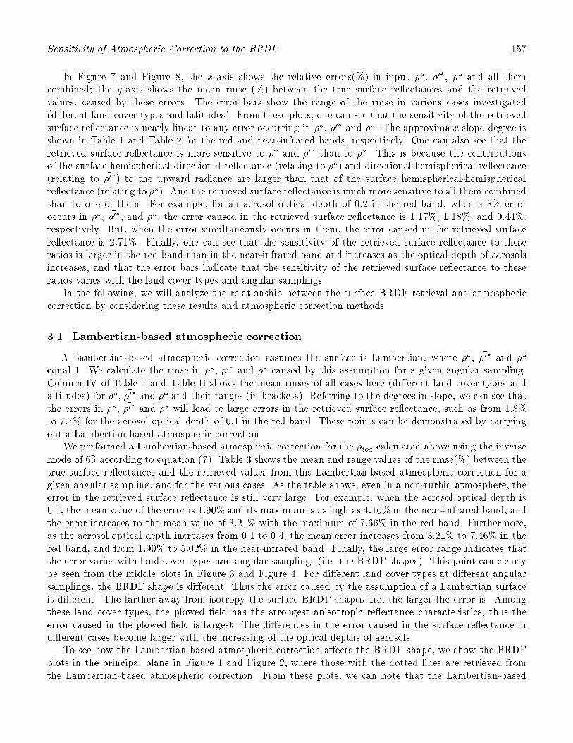
Sensitivity of Atmospheric Correction to the BRDF 157
In Figure 7 and Figure 8, the x-axis shows the relative errors(%) in input ���, ��0�, ���� and all themcombined; the y-axis shows the mean rmse (%) between the true surface re ectances and the retrievedvalues, caused by these errors. The error bars show the range of the rmse in various cases investigated(di�erent land cover types and latitudes). From these plots, one can see that the sensitivity of the retrievedsurface re ectance is nearly linear to any error occurring in ���, ��0� and ����. The approximate slope degree isshown in Table 1 and Table 2 for the red and near-infrared bands, respectively. One can also see that theretrieved surface re ectance is more sensitive to ��� and ��0� than to ����. This is because the contributionsof the surface hemispherical-directional re ectance (relating to ���) and directional-hemispherical re ectance(relating to ��0�) to the upward radiance are larger than that of the surface hemispherical-hemisphericalre ectance (relating to ����). And the retrieved surface re ectance is much more sensitive to all them combinedthan to one of them. For example, for an aerosol optical depth of 0:2 in the red band, when a 8% erroroccurs in ���, ��0�, and ����, the error caused in the retrieved surface re ectance is 1:17%, 1:18%, and 0:44%,respectively. But, when the error simultaneously occurs in them, the error caused in the retrieved surfacere ectance is 2:71%. Finally, one can see that the sensitivity of the retrieved surface re ectance to theseratios is larger in the red band than in the near-infrared band and increases as the optical depth of aerosolsincreases, and that the error bars indicate that the sensitivity of the retrieved surface re ectance to theseratios varies with the land cover types and angular samplings.
In the following, we will analyze the relationship between the surface BRDF retrieval and atmosphericcorrection by considering these results and atmospheric correction methods.
3.1. Lambertian-based atmospheric correction
A Lambertian-based atmospheric correction assumes the surface is Lambertian, where ���, ��0� and ����
equal 1. We calculate the rmse in ���, ��0� and ���� caused by this assumption for a given angular sampling.Column IV of Table 1 and Table II shows the mean rmses of all cases here (di�erent land cover types andaltitudes) for ���, ��0� and ���� and their ranges (in brackets). Referring to the degrees in slope, we can see thatthe errors in ���, ��0� and ���� will lead to large errors in the retrieved surface re ectance, such as from 1:8%to 7:7% for the aerosol optical depth of 0:1 in the red band. These points can be demonstrated by carryingout a Lambertian-based atmospheric correction.
We performed a Lambertian-based atmospheric correction for the �toa calculated above using the inversemode of 6S according to equation (7). Table 3 shows the mean and range values of the rmse(%) between thetrue surface re ectances and the retrieved values from this Lambertian-based atmospheric correction for agiven angular sampling, and for the various cases. As the table shows, even in a non-turbid atmosphere, theerror in the retrieved surface re ectance is still very large. For example, when the aerosol optical depth is0.1, the mean value of the error is 1:90% and its maximum is as high as 4:10% in the near-infrared band, andthe error increases to the mean value of 3:21% with the maximum of 7:66% in the red band. Furthermore,as the aerosol optical depth increases from 0.1 to 0.4, the mean error increases from 3:21% to 7:46% in thered band, and from 1:90% to 5:02% in the near-infrared band. Finally, the large error range indicates thatthe error varies with land cover types and angular samplings (i.e. the BRDF shapes). This point can clearlybe seen from the middle plots in Figure 3 and Figure 4. For di�erent land cover types at di�erent angularsamplings, the BRDF shape is di�erent. Thus the error caused by the assumption of a Lambertian surfaceis di�erent. The farther away from isotropy the surface BRDF shapes are, the larger the error is. Amongthese land cover types, the plowed �eld has the strongest anisotropic re ectance characteristics, thus theerror caused in the plowed �eld is largest. The di�erences in the error caused in the surface re ectance indi�erent cases become larger with the increasing of the optical depths of aerosols.
To see how the Lambertian-based atmospheric correction a�ects the BRDF shape, we show the BRDFplots in the principal plane in Figure 1 and Figure 2, where those with the dotted lines are retrieved fromthe Lambertian-based atmospheric correction. From these plots, we can note that the Lambertian-based
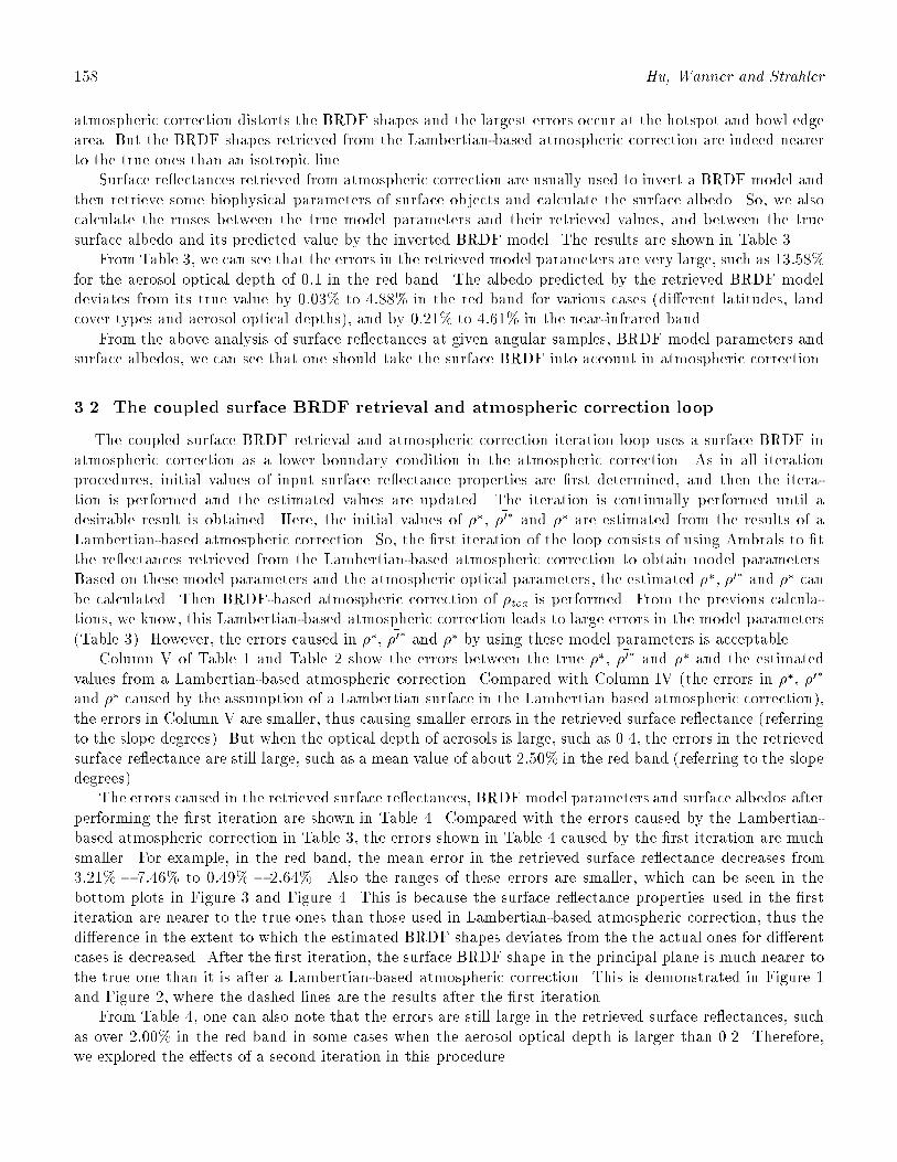
158 Hu, Wanner and Strahler
atmospheric correction distorts the BRDF shapes and the largest errors occur at the hotspot and bowl edgearea. But the BRDF shapes retrieved from the Lambertian-based atmospheric correction are indeed nearerto the true ones than an isotropic line.
Surface re ectances retrieved from atmospheric correction are usually used to invert a BRDF model andthen retrieve some biophysical parameters of surface objects and calculate the surface albedo. So, we alsocalculate the rmses between the true model parameters and their retrieved values, and between the truesurface albedo and its predicted value by the inverted BRDF model. The results are shown in Table 3.
From Table 3, we can see that the errors in the retrieved model parameters are very large, such as 13:58%for the aerosol optical depth of 0:1 in the red band. The albedo predicted by the retrieved BRDF modeldeviates from its true value by 0:03% to 4:88% in the red band for various cases (di�erent latitudes, landcover types and aerosol optical depths), and by 0:21% to 4:61% in the near-infrared band.
From the above analysis of surface re ectances at given angular samples, BRDF model parameters andsurface albedos, we can see that one should take the surface BRDF into account in atmospheric correction.
3.2. The coupled surface BRDF retrieval and atmospheric correction loop
The coupled surface BRDF retrieval and atmospheric correction iteration loop uses a surface BRDF inatmospheric correction as a lower boundary condition in the atmospheric correction. As in all iterationprocedures, initial values of input surface re ectance properties are �rst determined, and then the itera-tion is performed and the estimated values are updated. The iteration is continually performed until adesirable result is obtained. Here, the initial values of ���, ��0� and ���� are estimated from the results of aLambertian-based atmospheric correction. So, the �rst iteration of the loop consists of using Ambrals to �tthe re ectances retrieved from the Lambertian-based atmospheric correction to obtain model parameters.Based on these model parameters and the atmospheric optical parameters, the estimated ���, ��0� and ���� canbe calculated. Then BRDF-based atmospheric correction of �toa is performed. From the previous calcula-tions, we know, this Lambertian-based atmospheric correction leads to large errors in the model parameters(Table 3). However, the errors caused in ���, ��0� and ���� by using these model parameters is acceptable.
Column V of Table 1 and Table 2 show the errors between the true ���, ��0� and ���� and the estimatedvalues from a Lambertian-based atmospheric correction. Compared with Column IV (the errors in ���, ��0�
and ���� caused by the assumption of a Lambertian surface in the Lambertian based atmospheric correction),the errors in Column V are smaller, thus causing smaller errors in the retrieved surface re ectance (referringto the slope degrees). But when the optical depth of aerosols is large, such as 0.4, the errors in the retrievedsurface re ectance are still large, such as a mean value of about 2:50% in the red band (referring to the slopedegrees).
The errors caused in the retrieved surface re ectances, BRDF model parameters and surface albedos afterperforming the �rst iteration are shown in Table 4. Compared with the errors caused by the Lambertian-based atmospheric correction in Table 3, the errors shown in Table 4 caused by the �rst iteration are muchsmaller. For example, in the red band, the mean error in the retrieved surface re ectance decreases from3:21% � 7:46% to 0:49% � 2:64%. Also the ranges of these errors are smaller, which can be seen in thebottom plots in Figure 3 and Figure 4. This is because the surface re ectance properties used in the �rstiteration are nearer to the true ones than those used in Lambertian-based atmospheric correction, thus thedi�erence in the extent to which the estimated BRDF shapes deviates from the the actual ones for di�erentcases is decreased. After the �rst iteration, the surface BRDF shape in the principal plane is much nearer tothe true one than it is after a Lambertian-based atmospheric correction. This is demonstrated in Figure 1and Figure 2, where the dashed lines are the results after the �rst iteration.
From Table 4, one can also note that the errors are still large in the retrieved surface re ectances, suchas over 2:00% in the red band in some cases when the aerosol optical depth is larger than 0.2. Therefore,we explored the e�ects of a second iteration in this procedure.
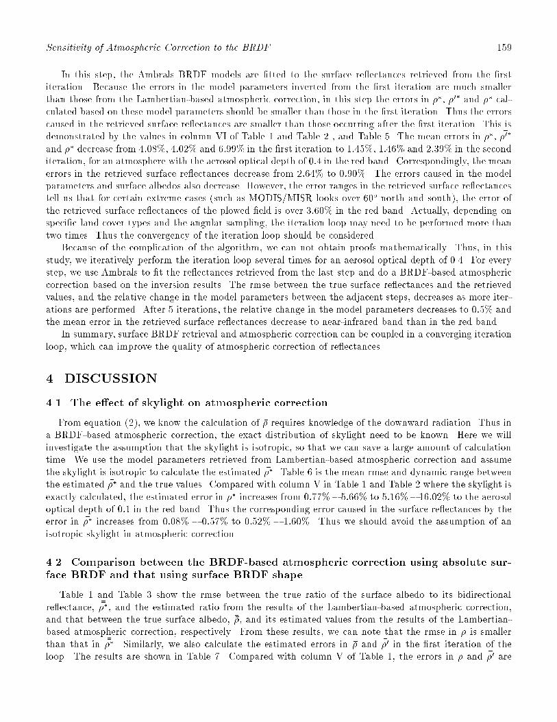
Sensitivity of Atmospheric Correction to the BRDF 159
In this step, the Ambrals BRDF models are �tted to the surface re ectances retrieved from the �rstiteration. Because the errors in the model parameters inverted from the �rst iteration are much smallerthan those from the Lambertian-based atmospheric correction, in this step the errors in ���, ��0� and ���� cal-culated based on these model parameters should be smaller than those in the �rst iteration. Thus the errorscaused in the retrieved surface re ectances are smaller than those occurring after the �rst iteration. This isdemonstrated by the values in column VI of Table 1 and Table 2 , and Table 5. The mean errors in ���, ��0�
and ���� decrease from 4:08%, 4:02% and 6:99% in the �rst iteration to 1:45%, 1:46% and 2:39% in the seconditeration, for an atmosphere with the aerosol optical depth of 0:4 in the red band. Correspondingly, the meanerrors in the retrieved surface re ectances decrease from 2:64% to 0:90%. The errors caused in the modelparameters and surface albedos also decrease. However, the error ranges in the retrieved surface re ectancestell us that for certain extreme cases (such as MODIS/MISR looks over 60o north and south), the error ofthe retrieved surface re ectances of the plowed �eld is over 3:60% in the red band. Actually, depending onspeci�c land cover types and the angular sampling, the iteration loop may need to be performed more thantwo times. Thus the convergency of the iteration loop should be considered.
Because of the complication of the algorithm, we can not obtain proofs mathematically. Thus, in thisstudy, we iteratively perform the iteration loop several times for an aerosol optical depth of 0.4. For everystep, we use Ambrals to �t the re ectances retrieved from the last step and do a BRDF-based atmosphericcorrection based on the inversion results. The rmse between the true surface re ectances and the retrievedvalues, and the relative change in the model parameters between the adjacent steps, decreases as more iter-ations are performed. After 5 iterations, the relative change in the model parameters decreases to 0:5% andthe mean error in the retrieved surface re ectances decrease to near-infrared band than in the red band.
In summary, surface BRDF retrieval and atmospheric correction can be coupled in a converging iterationloop, which can improve the quality of atmospheric correction of re ectances.
4. DISCUSSION
4.1. The e�ect of skylight on atmospheric correction
From equation (2), we know the calculation of �� requires knowledge of the downward radiation. Thus ina BRDF-based atmospheric correction, the exact distribution of skylight need to be known. Here we willinvestigate the assumption that the skylight is isotropic, so that we can save a large amount of calculationtime. We use the model parameters retrieved from Lambertian-based atmospheric correction and assumethe skylight is isotropic to calculate the estimated ���. Table 6 is the mean rmse and dynamic range betweenthe estimated ��� and the true values. Compared with column V in Table 1 and Table 2 where the skylight isexactly calculated, the estimated error in ��� increases from 0:77%� 5:66% to 5:16%� 16:02% to the aerosoloptical depth of 0:1 in the red band. Thus the corresponding error caused in the surface re ectances by theerror in ��� increases from 0:08% � 0:57% to 0:52%� 1:60%. Thus we should avoid the assumption of anisotropic skylight in atmospheric correction.
4.2. Comparison between the BRDF-based atmospheric correction using absolute sur-
face BRDF and that using surface BRDF shape
Table 1 and Table 3 show the rmse between the true ratio of the surface albedo to its bidirectionalre ectance, ����, and the estimated ratio from the results of the Lambertian-based atmospheric correction,and that between the true surface albedo, ���, and its estimated values from the results of the Lambertian-based atmospheric correction, respectively. From these results, we can note that the rmse in ��� is smallerthan that in ����. Similarly, we also calculate the estimated errors in �� and ��0 in the �rst iteration of theloop. The results are shown in Table 7. Compared with column V of Table 1, the errors in �� and ��0 are

160 Hu, Wanner and Strahler
smaller than those in ��� and ��0�. So a question remains, is the BRDF-based atmospheric correction basedon Equation (7) better than that based on Equation (1)? To answer this question, we analyze the sensitivityof the retrieved surface re ectance to ��, ��0 and ��� according to Equation (1) under the same simulationconditions as those in the above sensitivity analysis. Figure 7 shows the results in the red band. ComparingFigure 7 and Figure 5, one can see that the surface re ectance is more sensitive to ��, ��0 and ��� than to ���,��0� and ����. Thus even though the estimated errors in ��, ��0 and ��� are smaller than those in ���, ��0� and ����,the error caused in the surface re ectances is larger by the errors in ��, ��0 and ��� than by the errors in ���, ��0�
and ����. The BRDF-based atmospheric correction using the estimated surface BRDF shapes is better thanthat using absolute surface BRDF.
5. Conclusions
In this study, we analyze the sensitivity of atmospherically corrected re ectances to surface BRDF. Decou-pling atmospheric correction and the surface anisotropic BRDF leads to large errors in the retrieved surfacere ectances. In addition to atmospheric optical parameters, surface BRDF shape determines the size of theerror, varying from 2:41% to 11:64% in the red band for the atmosphere with the aerosol optical depth of0:2. The farther away from isotropy the BRDF shape is, the larger the error becomes. The surface BRDFretrieval and atmospheric correction can be coupled in a converging iteration loop. The initial values ofsurface re ectance properties are derived from the atmospheric correction with the assumption of a Lamber-tian surface. The accuracy of the estimated surface re ectance properties increases as more iterations areperformed, thus the error in the retrieved surface re ectance decreases. However, one or two iterations arealready su�cient to obtain a mean error of only 0.89% in the red band even with an atmospheric opticaldepth of 0:4.
As one notes, all the error values in this study are based on the assumption that the exact atmosphericoptical parameters are known. This does not hold in actual applications. In the future, we will furtheranalyze the e�ect of the uncertainty of atmospheric optical parameters on the sensitivity of atmosphericcorrection of re ectances to the surface BRDF.
We wish to thank Xiaowen Li, Crystal Schaaf, and other members of the MODIS BRDF/albedo team for
their support and numerous discussions. This work was supported by NASA under NAS5-31369.
REFERENCES
Asrar, Ghassem, Theory and Applications of Optical Remote Sensing, A Wiley-Interscience Publication,1989.
Case, R.M., F. de Ho�mane and G. Placzek, Introduction to the theory of neutron di�usion, vol.1, LosAlamos Scienti�c Laboratory, 1953.
Lee, T. Y. and Y. J. Kaufman, Non-Lambertian e�ects in remote sensing of surface re ectance and vege-tation index, IEEE trans. Geosci. Remote Sens., 24, 699-708, 1986.
Liang S. and A. H. Strahler, Calculation of the angular radiation distribution for a coupled atmosphereand canopy, IEEE trans. Geosci. Remote Sens., 31, 491-502, 1993.
Kaufman Y. J., A. Gitelson, A. Karnieli, E. Ganor, R. S. Fraser, T. Nakajima, S. Mattoo, and B. N.Holben, Size distribution and scattering phase function of aerosol particles retrieved from sky brightnessmeasurements, J. Geophys. Res., 100, 10341-10356, 1994.

Sensitivity of Atmospheric Correction to the BRDF 161
Kimes, D. S., A. G. Kerber and P. J. Seller, Dynamics of directional re ectance factor distribution forvegetation canopies, Appl. Opt., 22(9), 1364-1372, 1983.
Kimes, D. S., W. W. Newcomb, C. J. Tucker, I. S. Zonneveldt, W. van Wijngaarden, J. de Leeuw, andG. F. Epema, Directional re ectance factor distributions for cover types of Northern Africa, RemoteSens. Environ 18, 1-19,1985.
Kimes, D. S., W. W. Newcomb, R. F. Nelson, and J. B. Schutt, Directional re ectance distributions of ahardwood and a pine forest canopy, IEEE Trans. Geosci. Remote Sens. GE-24, 281-293, 1986.
Kriebel, K. T., Measured spectral bidirectional re ection properties of four vegetated surfaces, Appl. Op-tics, 17(2), 352-259, 1978.
Myneni, R. B. and J. Ross, Photon-Vegetation Interactions", Springer- Verlag, 1991.
Pinty, B., Verstraete, M. M. and Dickinso, R. E., A physical model for predicting bidirectional re ectancesover bare soil, Remote Sens. Env., 27, 273-288, 1989.
Strahler, A. H., Barnsley M. J., d'Entremont R., Hu B., Lewis P., Li X., Muller J., Schaaf, C. B., WannerW. and Zhang B., MODIS BRDF/ Albedo Product: Algorithm Theoretical Basis Document Version3.2, NASA EOS-MODIS, 1995.
Vermote, E. F., D. Tanre, Deuze, J. L. Herman, M. and Morcrette, J. J., Second Simulation of the SatelliteSignal in the Solar Spectrum (6S), 6S User Guide Version 0, NASA-Goddard Space Flight Center-Code923, Greenbelt, MD 20771, 1994.
Vermote, E. F., L. A. Remer, C. O. Justice, Y. J. Kaufman, and D. Tanre, Algorithm technical backgroundDocument: atmospheric correction algorithm, Modis Science Team and Associates, 1995.
Vermote, E. F., N. El Saleous, C. O. Justice, Y. J. Kaufman, J. L. Privette, L. Remer, J. C. Roger, andD. Tanre, Atmospheric correction of visible to middle infrared EOS-MODIS data over land surface:background, operational algorithm and validation, J. Geophys. Res., in press, 1996.
Wanner, W., X. Li, A. H. Strahler, On the derivation of kernels for kernel-driven models of bidirectionalre ectance, J. Geophys. Res., 100, 21077-21089, 1995.
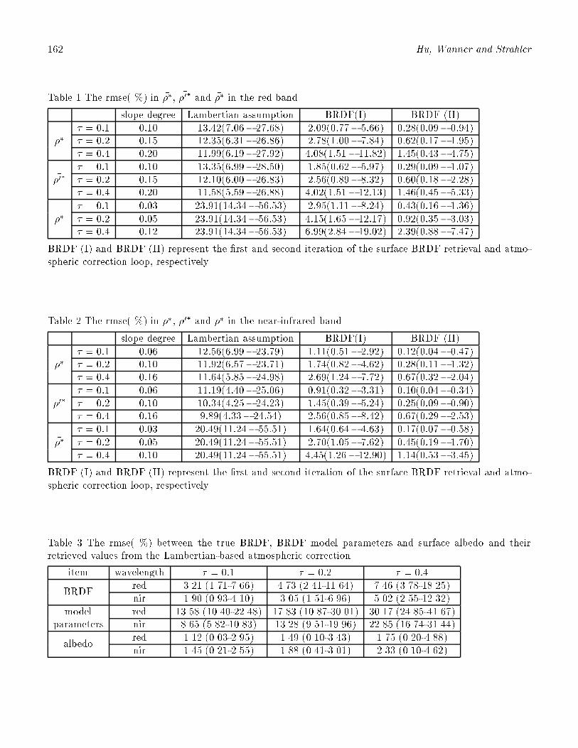
162 Hu, Wanner and Strahler
Table 1 The rmse( %) in ���, ��0� and ���� in the red band
slope degree Lambertian assumption BRDF(I) BRDF (II)
� = 0:1 0:10 13:42(7:06� 27:68) 2:09(0:77� 5:66) 0:28(0:09� 0:94)��� � = 0:2 0:15 12:35(6:31� 26:86) 2:78(1:00� 7:84) 0:62(0:17� 1:95)
� = 0:4 0:20 11:99(6:19� 27:92) 4:08(1:51� 11:82) 1:45(0:43� 4:75)
� = 0:1 0:10 13:35(6:99� 28:50) 1:85(0:62� 5:97) 0:29(0:09� 1:07)��0� � = 0:2 0:15 12:10(6:00� 26:83) 2:56(0:89� 8:32) 0:60(0:18� 2:28)
� = 0:4 0:20 11:58(5:59� 26:88) 4:02(1:51� 12:13) 1:46(0:45� 5:33)
� = 0:1 0:03 23:91(14:34� 56:53) 2:95(1:11� 8:24) 0:43(0:16� 1:36)���� � = 0:2 0:05 23:91(14:34� 56:53) 4:15(1:65� 12:17) 0:92(0:35� 3:03)
� = 0:4 0:12 23:91(14:34� 56:53) 6:99(2:84� 19:02) 2:39(0:88� 7:47)
BRDF (I) and BRDF (II) represent the �rst and second iteration of the surface BRDF retrieval and atmo-spheric correction loop, respectively.
Table 2 The rmse( %) in ���, ��0� and ���� in the near-infrared band
slope degree Lambertian assumption BRDF(I) BRDF (II)
� = 0:1 0:06 12:56(6:99� 23:79) 1:11(0:51� 2:92) 0:12(0:04� 0:47)��� � = 0:2 0:10 11:92(6:57� 23:71) 1:74(0:82� 4:62) 0:28(0:11� 1:32)
� = 0:4 0:16 11:64(5:85� 24:98) 2:69(1:24� 7:72) 0:67(0:32� 2:04)
� = 0:1 0:06 11:19(4:40� 25:06) 0:91(0:32� 3:31) 0:10(0:04� 0:34)��0� � = 0:2 0:10 10:34(4:25� 24:23) 1:45(0:39� 5:24) 0:25(0:09� 0:90)
� = 0:4 0:16 9:89(4:33� 24:54) 2:56(0:85� 8:42) 0:67(0:29� 2:53)
� = 0:1 0:03 20:49(11:24� 55:51) 1:64(0:64� 4:63) 0:17(0:07� 0:58)���� � = 0:2 0:05 20:49(11:24� 55:51) 2:70(1:05� 7:62) 0:45(0:19� 1:70)
� = 0:4 0:10 20:49(11:24� 55:51) 4:45(1:26� 12:90) 1:14(0:53� 3:45)
BRDF (I) and BRDF (II) represent the �rst and second iteration of the surface BRDF retrieval and atmo-spheric correction loop, respectively.
Table 3 The rmse( %) between the true BRDF, BRDF model parameters and surface albedo and theirretrieved values from the Lambertian-based atmospheric correction
item wavelength � = 0:1 � = 0:2 � = 0:4
red 3.21 (1.71-7.66) 4.73 (2.41-11.64) 7.46 (3.78-18.25)BRDF
nir 1.90 (0.93-4.10) 3.05 (1.51-6.96) 5.02 (2.55-12.32)
model red 13.58 (10.40-22.48) 17.83 (10.87-30.01) 30.17 (24.85-41.67)parameters nir 8.65 (5.82-10.83) 13.28 (9.51-19.96) 22.85 (16.74-31.44)
red 1.12 (0.03-2.95) 1.49 (0.10-3.43) 1.75 (0.20-4.88)albedo
nir 1.45 (0.21-2.55) 1.88 (0.41-3.01) 2.33 (0.10-4.62)

Sensitivity of Atmospheric Correction to the BRDF 163
Table 4 The rmse( %) between the true BRDF, BRDF model parameters and surface albedo and theirretrieved values from the �rst iteration of the coupled surface BRDF retrieval and atmospheric correctionloop
item wavelength � = 0:1 � = 0:2 � = 0:4
red 0.49 (0.16-1.85) 1.05 (0.32-3.92) 2.64 (0.84-9.08)BRDF
nir 0.17 (0.09-0.60) 0.45 (0.26-1.34) 1.25 (0.56-1.64)
model red 1.66 (1.12-2.65) 3.69 (2.56-5.69) 9.72 (6.99-14.49)parameters nir 0.74 (0.34-1.16) 1.87 (0.94-2.78) 5.17 (3.00-7.99)
red 0.36 (0.01-0.86) 0.68 (0.01-1.66) 1.33 (0.10-3.21)albedo
nir 0.15 (0.00-0.33) 0.32 (0.02-0.70) 0.70 (0.02-1.74)
Table 5 The rmse( %) between the true BRDF, BRDF model parameters and surface albedo and their re-trieved values from the second iterations of the coupled surface BRDF retrieval and atmospheric correctionloop
item wavelength � = 0:1 � = 0:2 � = 0:4
red 0.07 (0.02-0.31) 0.23 (0.07-0.99) 0.90 (0.25-3.63)BRDF
nir 0.02 (0.01-0.06) 0.07 (0.02-0.25) 0.34 (0.13-1.19)
model red 0.21 (0.11-0.46) 0.77 (0.43-1.14) 3.30 (1.96-8.11)parameters nir 0.06 (0.02-0.14) 0.26 (0.10-0.40) 1.25 (0.56-2.22)
red 0.06 (0.01-0.15) 0.15 (0.01-0.43) 0.48 (0.01-1.35)albedo
nir 0.02 (0.00-0.03) 0.05 (0.00-0.11) 0.23 (0.01-0.88)
Table 6 The rmse( %) in ��� in the �rst iteration under the assumption of an isotropic skylight
wavelength � = 0:1 � = 0:2 � = 0:4red 9.22 (5.16-16.02) 8.54 (4.29-15.76) 7.20 (3.48-12.33)
nir 10.03 (3.49-17.60) 9.33 (2.61-16.28) 8.22 (2.03-5.64)
Table 7 The rmse( %) in �� and ��0 in the red band in the �rst iteration of the coupled surface BRDF retrievaland atmospheric correction loop
� = 0:1 � = 0:2 � = 0:4�� 1.78 (0.80-4.56) 2.63 (1.28-5.17) 3.87 (2.15-8.10)��0 1.71 (0.81-4.36) 2.47 (1.34-5.00) 3.77 (2.21-7.94)
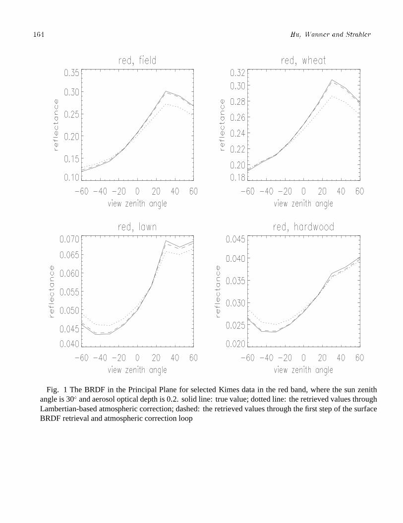
164 Hu, Wanner and Strahler
Fig. 1 The BRDF in the Principal Plane for selected Kimes data in the red band, where the sun zenithangle is 30o and aerosol optical depth is 0:2. solid line: true value; dotted line: the retrieved values throughLambertian-based atmospheric correction; dashed: the retrieved values through the first step of the surfaceBRDF retrieval and atmospheric correction loop

Sensitivity of Atmospheric Correction to the BRDF 165
Fig. 2 The BRDF in the Principal Plane for selected Kimes data in the near-infrared band, where the sunzenith angle is 30o and aerosol optical depth is 0:2. solid line: true value; dotted line: the retrieved valuesthrough Lambertian-based atmospheric correction; dashed: the retrieved values through the first step of thesurface BRDF retrieval and atmospheric correction loop
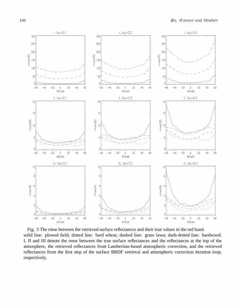
166 Hu, Wanner and Strahler
Fig. 3 The rmse between the retrieved surface reflectances and their true values in the red band.solid line: plowed field; dotted line: hard wheat; dashed line: grass lawn; dash-dotted line: hardwood.I, II and III denote the rmse between the true surface reflectances and the reflectances at the top of theatmosphere, the retrieved reflectances from Lambertian-based atmospheric correction, and the retrievedreflectances from the first step of the surface BRDF retrieval and atmospheric correction iteration loop,respectively.
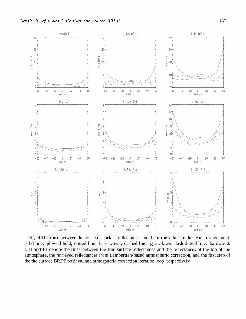
Sensitivity of Atmospheric Correction to the BRDF 167
Fig. 4 The rmse between the retrieved surface reflectances and their true values in the near-infrared band.solid line: plowed field; dotted line: hard wheat; dashed line: grass lawn; dash-dotted line: hardwood.I, II and III denote the rmse between the true surface reflectances and the reflectances at the top of theatmosphere, the retrieved reflectances from Lambertian-based atmospheric correction, and the first step ofthe the surface BRDF retrieval and atmospheric correction iteration loop, respectively.
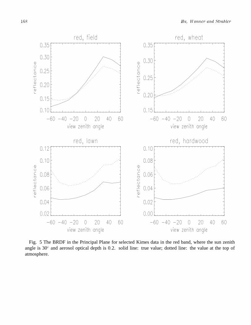
168 Hu, Wanner and Strahler
Fig. 5 The BRDF in the Principal Plane for selected Kimes data in the red band, where the sun zenithangle is 30o and aerosol optical depth is 0:2. solid line: true value; dotted line: the value at the top ofatmosphere.

Sensitivity of Atmospheric Correction to the BRDF 169
Fig. 6 The BRDF in the Principal Plane for selected Kimes data in the near-infrared band, where the sunzenith angle is 30o and aerosol optical depth is 0:2. solid line: true value; dotted line: the value at the topof atmosphere.

170 Hu, Wanner and Strahler
Fig. 7 The sensitivity of the retrieved surface reflectances to �̄�(I), �̄0�(II), ¯̄�� (III) and all of them togather(IV) in the red band

Sensitivity of Atmospheric Correction to the BRDF 171
Fig. 8 The sensitivity of the retrieved surface reflectances to �̄�(I), �̄0�(II), ¯̄�� (III), and all of them togather(IV) in the near infrared band

172 Hu, Wanner and Strahler
Fig. 9 The comparison between the sensitivity of the retrieved surface reflectances to �̄(I), �̄0(II), ¯̄� (III)(dashed lines) and the sensitivity of the retrieved surface reflectances to �̄�(I), �̄0�(II), ¯̄�� (III) (solid lines) inthe red band.

Global BRDF and Albedo Retrieval Over Land 173
APPENDIX E:
GLOBAL RETRIEVAL OF BIDIRECTIONAL REFLECTANCE AND
ALBEDO OVER LAND FROM EOSMODIS ANDMISR DATA: THE-
ORYAND ALGORITHM (PAPER BYWANNER ET AL., JGR, 1997)
174 Wanner et al.
Accepted for publication by JGR (1997) { will be revised slightly.
Global Retrieval of Bidirectional Re ectance and Albedo over LandFrom EOS MODIS and MISR Data: Theory and Algorithm
W. Wanner, A. H. Strahler, B. Hu
Department of Geography and Center for Remote Sensing, Boston University, Boston, Massachusetts.
P. LewisRemote Sensing Unit, University College London, London, UK.
J.-P. Muller
Department of Photogrammetry and Surveying, University College London, London, UK.
X. Li, C. L. Barker SchaafDepartment of Geography and Center for Remote Sensing, Boston University, Boston, Massachusetts.
M. J. Barnsley Department of Geography, University of Wales, Singleton Park, Swansea, SA2 8PP, UK.
Abstract
This paper describes the theory and the algorithm to be used in producing a global bidirectional re ectance distribution
function (BRDF) and albedo product from data to be acquired by the moderate resolution imaging spectroradiometer
(MODIS) and the multiangle imaging spectroradiometer (MISR), both to be launched in 1998 on the AM-1 satellite
platform as part of NASA's Earth Observing System (EOS). The product will be derived using the kernel-driven
semiempirical Ambrals BRDF model, utilizing �ve variants of kernel functions characterizing isotropic, volume and
surface scattering. The BRDF and the albedo of each pixel of the land surface will be modeled at a spatial resolution
of one kilometer and once every 16 days in seven spectral bands spanning the visible and the near-infrared. The BRDF
parameters retrieved and recorded in the MODIS BRDF/albedo product will be intrinsic surface properties decoupled
from the prevailing atmospheric state and hence suited for a wide range of applications requiring characterization of
the directional anisotropy of earth surface re ectance. A set of quality control ags accompanies the product. An
initial validation of the Ambrals model is demonstrated using a variety of �eld-measured data sets for several di�erent
land cover types.
1. Introduction
This paper reports on the status of the science and al-gorithms to be employed in the routine production of aglobal 1-km land surface bidirectional re ectance distri-bution function (BRDF) and albedo data product to begenerated beginning in mid-1998. This product will bederived from the combined data of the moderate reso-lution imaging spectroradiometer (MODIS) [Running etal., 1994] and the multiangle imaging spectroradiometer(MISR) [Diner et al., 1991], two key sensors of NASA'sEarth Observing System (EOS) on the AM-1 platform.
Produced through the MODIS project, it will be availablefor use in atmospheric correction problems, earth radia-tion budget studies, and climate and climate change in-vestigations. It will also allow some inference of land sur-face properties for use in global land cover classi�cationand biophysical databases for vegetation modeling. Fur-thermore, it will be employed in the angular correction ofMODIS and similar imagery.
Section 2 of this paper gives an overview of BRDFapplications, with an emphasis on the coupling betweenthe atmosphere and surface re ectance. In section 3, theMODIS BRDF/albedo product will be discussed with re-
Global BRDF and Albedo Retrieval Over Land 175
spect to sensor characteristics and the Ambrals BRDFmodels to be used. Section 4 introduces the algorithmthat was developed for the processing, explains the pro-cessing philosophy, and describes the product produced.Section 5 o�ers an outline of current model and plannedproduct validation, and discusses the possible relationshipof the BRDF model kernels used to land cover type. Thepaper closes with conclusions.
2. Multiangle E�ects in Remote
Sensing
2.1. Bidirectional Re ectance
The observation that the re ectance of most natural sur-faces is anisotropic in nature is relevant to remote sensingbecause under such circumstances the re ectance of a sur-face depends both on the viewing and on the illuminationangle. With natural scenes, this directional anisotropy iscaused by the way in which shadows cast by an ensemble ofobjects such as plants, buildings or topographic slopes arehidden or emerge as a function of the observation angle,and by the intrinsic directionality of material in the scene,for example the leaves of the plants. Mathematically, it isdescribed by the BRDF [Nicodemus et al., 1977].
Variations of view angle across images and betweenimages occur naturally due to a wide swath width (as forthe advanced very high resolution radiometer (AVHRR)or MODIS) or to along-track o�-nadir viewing capabili-ties (as for the along-track scanning radiometer, ATSR-2,or MISR). Variations in the solar angle are caused by vari-ations in the time of day, season and latitude of observa-tions, and are also determined by orbital characteristics ofthe satellite. Unless corrections for the BRDF are made,comparisons of surface re ectance observations across im-ages from such instruments or between them are di�cultor impossible. A simple example is given by the problemof mosaicking together AVHRR data from di�erent orbitsto obtain a composite image, where the orbital border willbe visible due to the di�erence in the sun-view geometryin the two or several parts (see Li et al. [1996] for anillustration).
The need to take BRDF e�ects into account when con-ducting land surface studies, for example land cover clas-si�cation, has increasingly been recognized [e.g., Wu etal., 1994; Cihlar et al., 1995; Gutman, 1994; Moody andStrahler, 1994]. It is known that current vegetation in-dices retain some angular e�ects due to the di�erences inthe BRDF of di�erent wavebands [e.g., Wu et al., 1994].It may even be desirable to standardize observations toangles where no observations were acquired, for exampleto nadir view and/or sun angle [Leroy and Roujean, 1994].
The BRDF may also be used to derive albedos, which
are mathematically de�ned as weighted integrals (aver-ages) of the BRDF. Surface albedos play an important rolein global and regional climate since they determine the sur-face energy balance, for example the heat uxes linked toevapotranspiration [Kustas et al., 1989]. The BRDF andits integrals are also important for atmospheric correctionin remote sensing [Kaufman, 1989], where errors of up to10 percent or more may be made when BRDF e�ects aredisregarded. We will discuss albedos and atmospheric cor-rection in more detail further on. Recently there have alsobeen indications that knowledge of the BRDF function canbe valuable in cloud detection [d'Entremont et al., 1995,1996; see also DiGirolamo and Davies, 1994], opening upthe possibility of improved cloud detection in the absenceof thermal data.
Finally, the BRDF can be interpreted to infer landsurface properties. Since the angular dependence of there ectance is driven by the optical properties of the scat-tering medium and by its three-dimensional structure, onemay attempt to retrieve the dominant parameters describ-ing these properties from the observed BRDF functions.
Initially, such retrievals will be experimental, and themain focus of BRDF/albedo work will be on semiempiricaldescriptors of the BRDF that can be used for angle cor-rections and albedo calculations without requiring detailedphysical modeling of the scene viewed. This is the pathtaken by the MODIS BRDF/albedo product. As moreexperience is accumulated, however, and as more com-puter power becomes available, more elaborate retrievalsof physical parameters may be attempted [Goel, 1989;Pinty and Verstraete, 1991]. The MODIS land cover prod-uct [Strahler et al., 1995b] will make use of re ectancescorrected for angular e�ects but will also take into consid-eration the observed BRDF shape itself.
2.2. Surface BRDF-Atmosphere Coupling
Atmospheric correction algorithms for operational process-ing are commonly based on expressing the total transmit-tance of radiation from the top of the atmosphere to theground as the sum of a direct and a di�use component (seeKaufman [1989] for a general treatment of atmosphericcorrection in remote sensing). One then arrives at expres-sions such as the one suggested by Li [cf. Strahler et al.,1995a], which is similar to the formulation to be used forMODIS atmospheric correction in the visible and near-infrared [see Vermote et al., 1995, 1996]. We have:
�toa = �path +t(�s)Rt(�v) � e��=�s jRje��=�v
1� �s�a; (1)
where �s is the cosine of the solar zenith angle, �v that ofthe view zenith angle, �toa the re ectance at the top of theatmosphere, �path the re ectance due to path radiance, �athe downward hemispherical re ectance of the atmosphere
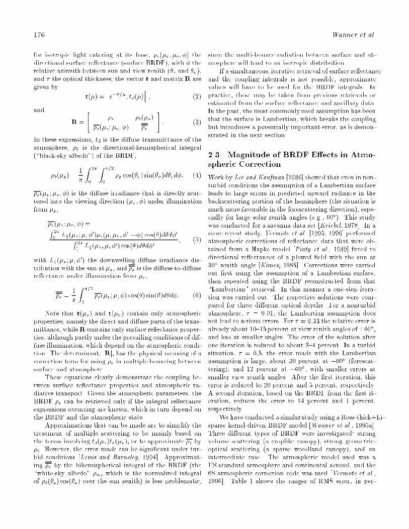
176 Wanner et al.
for isotropic light entering at its base, �s(�s; �v; �) thedirectional surface re ectance (surface BRDF), with � therelative azimuth between sun and view zenith (�s and �v),and � the optical thickness; the vector t and matrixR aregiven by
t(�) =he��=�; td(�)
i; (2)
and
R =
"�s �b(�s)
�s(�s;�v; �) �s
#: (3)
In these expressions, td is the di�use transmittance of theatmosphere, �b is the directional-hemispherical integral(\black-sky albedo") of the BRDF,
�b(�s) =1
�
Z2�
0
Z �=2
0
�s cos(�v) sin(�v)d�vd�; (4)
�s(�s;�v; �) is the di�use irradiance that is directly scat-tered into the viewing direction (�v; �) under illuminationfrom �s,
�s(�s;�v; �) =R2�
0L#(�s;�; �
0)�s(�; �v; �0 � �) cos(�)d�d�0R
2�
0L#(�s;�; �0) cos(�)d�d�0
; (5)
with L#(�s;�; �0) the downwelling di�use irradiance dis-tribution with the sun at �s, and �s is the di�use-to-di�usere ectance under illumination from �s,
�s =1
�
Z �=2
0
�s(�s;�; �) cos(�) sin(�)d�d�: (6)
Note that t(�s) and t(�v) contain only atmosphericproperties, namely the direct and di�use parts of the trans-mittance, whileR contains only surface re ectance proper-ties, although partly under the prevailing conditions of dif-fuse illumination, which depend on the atmospheric condi-tion. The determinant, jRj, has the physical meaning of acorrection term for using �s in multiple bouncing betweensurface and atmosphere.
These equations clearly demonstrate the coupling be-tween surface re ectance properties and atmospheric ra-diative transport. Given the atmospheric parameters, theBRDF �s can be retrieved only if the integral re ectanceexpressions occurring are known, which in turn depend onthe BRDF and the atmospheric state.
Approximations that can be made are to simplify thetreatment of multiple scattering to be mainly based onthe terms involving td(�s)td(�v), or to approximate �s by�b. However, the error made can be signi�cant under tur-bid conditions [Lewis and Barnsley, 1994]. Approximat-ing �s by the bihemispherical integral of the BRDF (the\white-sky albedo" �w, which is the normalized integralof �b(�s) cos(�s) over the sun zenith) is less problematic,
since the multi-bounce radiation between surface and at-mosphere will tend to an isotropic distribution.
If a simultaneous, iterative retrieval of surface re ectanceand the coupling integrals is not possible, approximatevalues will have to be used for the BRDF integrals. Inpractice, these may be taken from previous retrievals orestimated from the surface re ectance and ancillary data.In the past, the most commonly used assumption has beenthat the surface is Lambertian, which breaks the couplingbut introduces a potentially important error, as is demon-strated in the next section.
2.3. Magnitude of BRDF E�ects in Atmo-
spheric Correction
Work by Lee and Kaufman [1986] showed that even in non-turbid conditions the assumption of a Lambertian surfaceleads to large errors in predicted upward radiance in thebackscattering portion of the hemisphere (the situation ismuch more favorable in the forescattering direction), espe-cially for large solar zenith angles (e.g., 60�). This studywas conducted for a savanna data set [Kriebel, 1978]. In amore recent study, Vermote et al. [1995, 1996] performedatmospheric corrections of re ectance data that were ob-tained from a Hapke model [Pinty et al., 1989] �tted todirectional re ectances of a plowed �eld with the sun at30� zenith angle [Kimes, 1985]. Corrections were carriedout �rst using the assumption of a Lambertian surface,then repeated using the BRDF reconstructed from that\Lambertian" retrieval. In this manner a one-step itera-tion was carried out. The respective solutions were com-pared for three di�erent optical depths. For a nonturbidatmosphere, � = 0:01, the Lambertian assumption doesnot lead to serious errors. For � = 0:23 the relative error isalready about 10{15 percent at view zenith angles of �60�,and less at smaller angles. The error of the solution afterone iteration is reduced to about 3{4 percent. In a turbidsituation, � = 0:5, the error made with the Lambertianassumption is large, about 30 percent at +60� (forescat-tering), and 12 percent at �60�, with smaller errors atsmaller view zenith angles. After the �rst iteration, thiserror is reduced to 20 percent and 5 percent, respectively.A second iteration, based on the BRDF from the �rst it-eration, reduces the error to 14 percent and 1 percent,respectively.
We have conducted a similar study using a Ross-thick+Li-sparse kernel-driven BRDF model [Wanner et al., 1995a].Three di�erent types of BRDF were investigated: strongvolume scattering (a croplike canopy), strong geometric-optical scattering (a sparse woodland canopy), and anintermediate case. The atmospheric model used was aUS standard atmosphere and continental aerosol, and the6S atmospheric correction code was used [Vermote et al.,1996]. Table 1 shows the ranges of RMS error, in per-
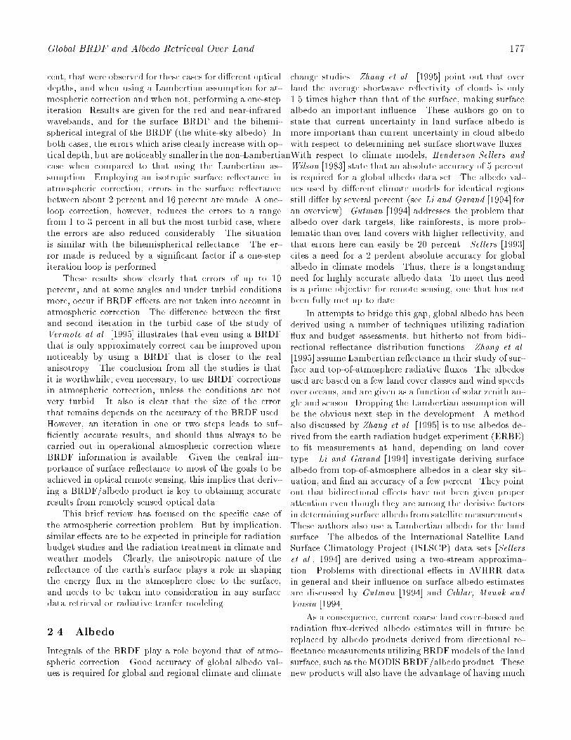
Global BRDF and Albedo Retrieval Over Land 177
cent, that were observed for these cases for di�erent opticaldepths, and when using a Lambertian assumption for at-mospheric correction and when not, performing a one-stepiteration. Results are given for the red and near-infraredwavebands, and for the surface BRDF and the bihemi-spherical integral of the BRDF (the white-sky albedo). Inboth cases, the errors which arise clearly increase with op-tical depth, but are noticeably smaller in the non-Lambertiancase when compared to that using the Lambertian as-sumption. Employing an isotropic surface re ectance inatmospheric correction, errors in the surface re ectancebetween about 2 percent and 16 percent are made. A one-loop correction, however, reduces the errors to a rangefrom 1 to 3 percent in all but the most turbid case, wherethe errors are also reduced considerably. The situationis similar with the bihemispherical re ectance. The er-ror made is reduced by a signi�cant factor if a one-stepiteration loop is performed.
These results show clearly that errors of up to 10percent, and at some angles and under turbid conditionsmore, occur if BRDF e�ects are not taken into account inatmospheric correction. The di�erence between the �rstand second iteration in the turbid case of the study ofVermote at al. [1995] illustrates that even using a BRDFthat is only approximately correct can be improved uponnoticeably by using a BRDF that is closer to the realanisotropy. The conclusion from all the studies is thatit is worthwhile, even necessary, to use BRDF correctionsin atmospheric correction, unless the conditions are notvery turbid. It also is clear that the size of the errorthat remains depends on the accuracy of the BRDF used.However, an iteration in one or two steps leads to suf-�ciently accurate results, and should thus always to becarried out in operational atmospheric correction whereBRDF information is available. Given the central im-portance of surface re ectance to most of the goals to beachieved in optical remote sensing, this implies that deriv-ing a BRDF/albedo product is key to obtaining accurateresults from remotely sensed optical data.
This brief review has focused on the speci�c case ofthe atmospheric correction problem. But by implication,similar e�ects are to be expected in principle for radiationbudget studies and the radiation treatment in climate andweather models. Clearly, the anisotropic nature of there ectance of the earth's surface plays a role in shapingthe energy ux in the atmosphere close to the surface,and needs to be taken into consideration in any surfacedata retrieval or radiative tranfer modeling.
2.4. Albedo
Integrals of the BRDF play a role beyond that of atmo-spheric correction. Good accuracy of global albedo val-ues is required for global and regional climate and climate
change studies. Zhang et al. [1995] point out that overland the average shortwave re ectivity of clouds is only1.5 times higher than that of the surface, making surfacealbedo an important in uence. These authors go on tostate that current uncertainty in land surface albedo ismore important than current uncertainty in cloud albedowith respect to determining net surface shortwave uxes.With respect to climate models, Henderson-Sellers andWilson [1983] state that an absolute accuracy of 5 percentis required for a global albedo data set. The albedo val-ues used by di�erent climate models for identical regionsstill di�er by several percent (see Li and Garand [1994] foran overview). Gutman [1994] addresses the problem thatalbedo over dark targets, like rainforests, is more prob-lematic than over land covers with higher re ectivity, andthat errors here can easily be 20 percent. Sellers [1993]cites a need for a 2 perdent absolute accuracy for globalalbedo in climate models. Thus, there is a longstandingneed for highly accurate albedo data. To meet this needis a prime objective for remote sensing, one that has notbeen fully met up to date.
In attempts to bridge this gap, global albedo has beenderived using a number of techniques utilizing radiation ux and budget assessments, but hitherto not from bidi-rectional re ectance distribution functions. Zhang et al.[1995] assume Lambertian re ectance in their study of sur-face and top-of-atmosphere radiative uxes. The albedosused are based on a few land cover classes and wind speedsover oceans, and are given as a function of solar zenith an-gle and season. Dropping the Lambertian assumption willbe the obvious next step in the development. A methodalso discussed by Zhang et al. [1995] is to use albedos de-rived from the earth radiation budget experiment (ERBE)to �t measurements at hand, depending on land covertype. Li and Garand [1994] investigate deriving surfacealbedo from top-of-atmosphere albedos in a clear sky sit-uation, and �nd an accuracy of a few percent. They pointout that bidirectional e�ects have not been given properattention even though they are among the decisive factorsin determining surface albedo from satellite measurements.These authors also use a Lambertian albedo for the landsurface. The albedos of the International Satellite LandSurface Climatology Project (ISLSCP) data sets [Sellerset al., 1994] are derived using a two-stream approxima-tion. Problems with directional e�ects in AVHRR datain general and their in uence on surface albedo estimatesare discussed by Gutman [1994] and Cihlar, Manak andVoisin [1994].
As a consequence, current coarse land cover-based andradiation ux-derived albedo estimates will in future bereplaced by albedo products derived from directional re- ectance measurements utilizing BRDFmodels of the landsurface, such as the MODIS BRDF/albedo product. Thesenew products will also have the advantage of having much

178 Wanner et al.
�ner spatial resolution than that of current data (2.5� �2.5� for ERBE; 1� � 1� for the ISLSCP data base). Thiswill allow not only a closer correlation of albedos with landcover classes, which is needed for parameterizations in theland surface schemes of climate models, but also quan-ti�cations of subgrid variability and derivation of bettercoarse-scale averages.
3. The MODIS BRDF/Albedo Prod-
uct
3.1. Product Outline
The MODIS BRDF/albedo product will provide the fullsurface BRDF as well as black-sky (directional) and white-sky (di�use) albedos, these albedos being intrinsic surfacealbedos. It will be produced from combining MODIS andMISR data, at a spatial resolution of 1 km, and over landonly, globally. BDRF and albedos will be provided in 7spectral bands ranging from 0.47 to 2.13�m (see Runninget al. [1994]) and in three broadbands ranging from 0.3to 0.7�m, from 0.7 to 3.0�m, and from 0.3 to 3.0�m. Theproduct will be produced once every 16 days (the EOS-AM-1 platform and MISR 2-look repeat rate) and will bebased on the semiempirical Ambrals BRDF model [Wan-ner et al., 1995a; Strahler et al., 1995a; Lewis, 1995].Results from inverting the empirical modi�ed WalthallBRDF model [Walthall et al., 1985; Nilson and Kuusk,1989] will also be recorded. A separate quarter-degree res-olution product will be provided for global modeling pur-poses. This product will also carry information on sub-scale variability. Principal Investigators on the MODISBRDF/albedo product are A. H. Strahler of Boston Uni-versity and J.-P. Muller of University College London.
3.2. Angular Sampling from MODIS and
MISR
Two key issues for a BRDF/albedo product are the angu-lar sampling coverage available and the expected rate ofloss of angular data due to cloud cover. Angular samplingis given by instrumental and orbital characteristics [Barns-ley et al., 1994]. The EOS-AM-1 platform carrying bothMODIS and MISR will have a polar orbit with a 10:30morning equatorial crossing time. The PM-1 platform, tobe launched in the year 2000 with a second MODIS sen-sor, will have a 13:30 early afternoon crossing time. Datafrom this second MODIS will be included in the MODISBRDF/albedo processing chain once it is available.
The MODIS sensor will image the earth's surface across-track with a swath width of 2330 km [Running et al., 1994].The viewing zenith angle will vary between �55�, or about�61� at the surface. The repeat cycle is two days at most,
and less than one day at latitudes greater than about 30�.Orbital overlap thus makes it well suited for accumulatingmultiangle re ectance data over a period of time. Spa-tial resolution at nadir is 250 meters for the red and nearinfrared bands and 500 meters for the other land bands.
MISR will image along-track using nine separate push-broom cameras [Diner et al., 1991]. Four of these areaft-looking, four fore-pointing, and one is nadir-viewing.Observations will be made in four spectral bands at visi-ble and near infrared wavelengths that are similar to thoseof MODIS. The potential spatial resolution of MISR ob-servations is 275 m, but data will be made available at astandard spatial resolution of 1.1 km. MISR's swath widthis 364 km, allowing for a 9-day global repeat cycle, withthe 2-repeat cycle being 16 (not 18) days at the equator.
Angular sampling su�cient for BRDF model inver-sions will be achieved by combining data from MODISand MISR in the four corresponding spectral bands, andby accumulating data over a period of 16 days. In theabsence of clouds, this leads to between 30 multiangularobservations available at the equator, and about 55 ob-servations at 60 degrees latitude, subject to variation withseason. Using a coarse statistic of mean global cloud coverprobability [Wylie and Menzel, 1989; Wylie et al., 1994]as a function of latitude, one may predict that generallyabout 15 to 20 multiangular observations will be availableat all latitudes except at the equator, where abundance ofcloudy conditions is likely to create problems.
With this number of observations available on average,su�cient angular coverage for a BRDF model inversion isto be expected in most cases. Since MODIS scans across-track and MISR along-track, the respective views will gen-erally represent di�erent parts of the BRDF [Barnsley etal, 1994]. When one sensor views the cross-principal planeof the BRDF, the other views the principal plane, and viceversa. Figure 1 illustrates this, showing two typical casesfor a particular latitude and time of year. With two sweepsacross it, sampling of the viewing hemisphere is good inall cases. Sampling of the illumination hemisphere, how-ever, is limited. Any one string of MISR data is acquiredfor only one solar zenith angle, while the MODIS observa-tions display a small but valuable variation in that angleduring the sampling period.
3.3. Kernel-Based SemiempiricalBRDFMod-
els
The MODIS BRDF/albedo product will be based on asemiempirical, kernel-based modeling approach introducedby Roujean et al. [1992] for top-down BRDF modeling.Mathematically, this type of model has the following form(here using two kernels and a constant):
R(�i; �v; �) = fi + fvkv(�i; �v; �) + fsks(�i; �v; �); (7)

Global BRDF and Albedo Retrieval Over Land 179
where R is the re ectance, kv and ks are kernel functions,and f are the weights of these functions (the model pa-rameters). The kernels depend only on the viewing andillumination geometry. They describe basic BRDF shapesinto which the full BRDF may be decomposed.
In this kernel-based BRDF model, the BRDF is givenas a linear superposition of kernel shapes, which are chosento represent di�erent types of scattering with typical in u-ences on the BRDF. In the above formulation, for example,kv stands for volume scattering as described by radiativetransfer theories, and ks for surface scattering as derivedfrom geometric-optical theories. The kernel that goes withthe constant fi is the isotropic Lambertian kernel, unity.Although the kernel functions used can be empirical (as inthe Walthall model [Walthall et al., 1985]), they are bestderived from a physical theory through approximation,making the resulting model semiempirical. Mathemati-cally, the weights f may be expressed in terms of physicalproperties of a scene, such as leaf area index, shape andheight of trees, surface re ectance, etc. Through inver-sion, however, only the three quantities f are retrieved,providing the relative in uence of the respective type ofscattering on the directional signal observed, and allowinga rough characterization of the structural characteristicsof the surface observed.
The kernel-based approach to BRDF modeling hasbeen discussed and justi�ed by Roujean et al. [1992] andWanner et al. [1995a]. Depending on the scene, it maybe understood in di�erent ways. In a mixed scene com-posed of two areas with di�erent BRDFs, for example agrassland-forest mixed pixel, the superposition representsthe respective areal contributions of the mainly shadow-driven (geometric-optical) BRDF of the forest and the tur-bid medium-type BRDF of the grassland. Adjacency ef-fects are neglected, which is admissible unless the mosaicis very �ne or the zenith angle very large. But even ina homogeneous scene, volume and surface scattering maystill be both present. For example, in a forest canopythe geometric scattering is given by the inter-crown gaps,whereas the volume scattering is given by the gaps be-tween the leaves. The superposition then describes �rstand second-order scattering, while neglecting the couplingof the two. From a practical standpoint, it is perhapsmost accurate to say that the BRDF observed is decom-posed into the two components represented by the twobasic types of scattering. Volume and surface scatteringproduce BRDF functions that are semi-orthogonal due toan increase in re ectance with zenith angle in the formerand a decrease in the latter case.
Kernel-driven models have been proven successful inapplication to AVHRR, advanced solid state array spectro-radiometer (ASAS), laboratory and �eld-measured multi-angular re ectance data and have been shown to �t ob-served BRDF data well [ Roujean et al., 1992; Leroy and
Roujean, 1994; Wu et al., 1995; Wanner et al., 1995b;[Privette and Vermote, 1995; Strahler et al., 1995c; Li etal., 1996; Barnsley et al., 1996b; Hu et al., 1996; Whiteet al., 1996]. Some examples of the latter will be given insection 5. A kernel-based model is also being used for theBRDF/albedo product of the polarization and directional-ity of the earth's radiation (POLDER) project [Deschampset al., 1994; Leroy et al., 1996].
3.4. The Ambrals BRDF Model
The kernel-based BRDF model to be used for productionof the MODIS BRDF/albedo product was chosen to bethe Ambrals BRDF (Algorithm for MODIS bidirectionalre ectance anisotropy of the land surface) BRDF model,as de�ned by the kernels used in it. The rationale forchoosing this model is given in section 3.5. The kernelsused are based on theory by Roujean et al. [1992], Ross[1981], Li and Strahler [1992], Li [Strahler et al., 1994;Wanner et al., 1995a] and Cox and Munk [1954].
The Ambrals model provides two choices each for thevolume scattering and the surface scattering kernel. Thekernels to be used in a particular case depend on thecharacteristics of the multiangular observations available.The two kernel expressions derived for volume scatteringare based on two di�erent approximations to a single-scattering radiative transfer theory of Ross [1981], one forlarge values of the leaf area index (\thick" approxima-tion) [Roujean et al., 1992], one for small values (\thin"approximation) [Wanner et al., 1995a]. For geometric sur-face scattering, two types of Li-kernels are available. Thesewere derived from the geometric-optical mutual shadowingBRDF model for forest canopies by Li and Strahler [1992].The �rst of these is an approximation for \sparse" spacingof discrete objects (crowns), the second for \dense" spac-ing of objects (crowns) [Strahler et al., 1994; Wanner et
al., 1995a]. The Li-sparse kernel is mainly driven by theway shadows emerge and are hidden in the scene, while theLi-dense kernel is dominated by the sunlit crowns as seenunder conditions of mutual shadowing in both viewingand illumination directions. For MODIS BRDF/albedoprocessing, the Li-sparse kernel is formulated to representspheroids that are relatively close to the ground (b=r =1, h=b = 2, where b is the crown vertical radius, r thecrown horizontal radius, and h the height to center-of-crown). The Li-dense kernel is formulated to representprolate crowns that are situated some distance above theground (b=r = 2:5, h=b = 2). For general use of theAmbrals model, other choices of these parameters can bemade.
In cases where the forward-scattering direction of theBRDF has been sampled, a Cox-Munk kernel has been de-veloped [Strahler et al., 1995a, update] to model contribu-tions from sub-resolution water bodies, ooded �elds, and
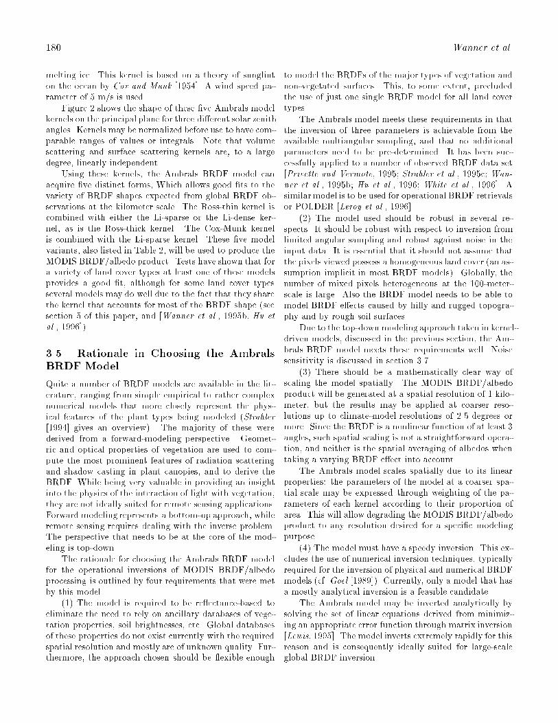
180 Wanner et al.
melting ice. This kernel is based on a theory of sunglinton the ocean by Cox and Munk [1954]. A wind speed pa-rameter of 5 m/s is used.
Figure 2 shows the shape of these �ve Ambrals modelkernels on the principal plane for three di�erent solar zenithangles. Kernels may be normalized before use to have com-parable ranges of values or integrals. Note that volumescattering and surface scattering kernels are, to a largedegree, linearly independent.
Using these kernels, the Ambrals BRDF model canacquire �ve distinct forms, Which allows good �ts to thevariety of BRDF shapes expected from global BRDF ob-servations at the kilometer scale. The Ross-thin kernel iscombined with either the Li-sparse or the Li-dense ker-nel, as is the Ross-thick kernel. The Cox-Munk kernelis combined with the Li-sparse kernel. These �ve modelvariants, also listed in Table 2, will be used to produce theMODIS BRDF/albedo product. Tests have shown that fora variety of land cover types at least one of these modelsprovides a good �t, although for some land cover typesseveral models may do well due to the fact that they sharethe kernel that accounts for most of the BRDF shape (seesection 5 of this paper, and [Wanner et al., 1995b, Hu etal., 1996]).
3.5. Rationale in Choosing the Ambrals
BRDF Model
Quite a number of BRDF models are available in the lit-erature, ranging from simple empirical to rather complexnumerical models that more closely represent the phys-ical features of the plant types being modeled (Strahler[1994] gives an overview). The majority of these werederived from a forward-modeling perspective. Geomet-ric and optical properties of vegetation are used to com-pute the most prominent features of radiation scatteringand shadow casting in plant canopies, and to derive theBRDF. While being very valuable in providing an insightinto the physics of the interaction of light with vegetation,they are not ideally suited for remote sensing applications.Forward modeling represents a bottom-up approach, whileremote sensing requires dealing with the inverse problem.The perspective that needs to be at the core of the mod-eling is top-down.
The rationale for choosing the Ambrals BRDF modelfor the operational inversions of MODIS BRDF/albedoprocessing is outlined by four requirements that were metby this model.
(1) The model is required to be re ectance-based toeliminate the need to rely on ancillary databases of vege-tation properties, soil brightnesses, etc. Global databasesof these properties do not exist currently with the requiredspatial resolution and mostly are of unknown quality. Fur-thermore, the approach chosen should be exible enough
to model the BRDFs of the major types of vegetation andnon-vegetated surfaces. This, to some extent, precludedthe use of just one single BRDF model for all land covertypes.
The Ambrals model meets these requirements in thatthe inversion of three parameters is achievable from theavailable multiangular sampling, and that no additionalparameters need to be pre-determined. It has been suc-cessfully applied to a number of observed BRDF data set[Privette and Vermote, 1995; Strahler et al., 1995c; Wan-ner et al., 1995b; Hu et al., 1996; White et al., 1996]. Asimilarmodel is to be used for operational BRDF retrievalsor POLDER [Leroy et al., 1996].
(2) The model used should be robust in several re-spects. It should be robust with respect to inversion fromlimited angular sampling and robust against noise in theinput data. It is essential that it should not assume thatthe pixels viewed possess a homogeneous land cover (an as-sumption implicit in most BRDF models). Globally, thenumber of mixed pixels heterogeneous at the 100-meter-scale is large. Also the BRDF model needs to be able tomodel BRDF e�ects caused by hilly and rugged topogra-phy and by rough soil surfaces.
Due to the top-downmodeling approach taken in kernel-driven models, discussed in the previous section, the Am-brals BRDF model meets these requirements well. Noisesensitivity is discussed in section 3.7.
(3) There should be a mathematically clear way ofscaling the model spatially. The MODIS BRDF/albedoproduct will be generated at a spatial resolution of 1 kilo-meter, but the results may be applied at coarser reso-lutions up to climate-model resolutions of 2.5 degrees ormore. Since the BRDF is a nonlinear function of at least 3angles, such spatial scaling is not a straightforward opera-tion, and neither is the spatial averaging of albedos whentaking a varying BRDF e�ect into account.
The Ambrals model scales spatially due to its linearproperties: the parameters of the model at a coarser spa-tial scale may be expressed through weighting of the pa-rameters of each kernel according to their proportion ofarea. This will allow degrading the MODIS BRDF/albedoproduct to any resolution desired for a speci�c modelingpurpose.
(4) The model must have a speedy inversion. This ex-cludes the use of numerical inversion techniques, typicallyrequired for the inversion of physical and numerical BRDFmodels (cf. Goel [1989]). Currently, only a model that hasa mostly analytical inversion is a feasible candidate.
The Ambrals model may be inverted analytically bysolving the set of linear equations derived from minimiz-ing an appropriate error function through matrix inversion[Lewis, 1995]. The model inverts extremely rapidly for thisreason and is consequently ideally suited for large-scaleglobal BRDF inversion.

Global BRDF and Albedo Retrieval Over Land 181
3.6. Albedo From MODIS
The in uence of atmospheric state on the radiative uxesat the surface becomes an issue when deriving albedo.Albedo is de�ned as the ratio between the hemispheri-cal upwelling and downwelling uxes, the latter dependingon the amount of di�use scattering occurring in the atmo-sphere due to its aerosol and water vapor load. This makesthe albedo itself dependent on the atmospheric state atthe time of observation. Albedo in this form, while char-acterizing accurately the radiative uxes at the time of ob-servation, is not directly usable in biospheric and climatemodeling, where the atmosphere applied and/or computedmay be di�erent from that observed and may vary as asimulation proceeds. What is needed for modeling is anaverage or hemispherical re ectance in form of an intrin-sic surface property that is not dependent on a particularatmosphere and time.
In order to meet this demand, the MODIS BRDF/albedoproduct will provide two measures of albedo in form of thedirectional-hemispherical and bihemispherical integrals ofthe BRDF, derived through the Ambrals BRDF modelfrom atmospherically corrected re ectances. These albedomeasures then are intrinsic properties of the surface. Theyrepresent the following two cases. The directional-hemisphericalintegral (4), called the \black-sky albedo," represents thecase of single-beam irradiation in the absence of di�useskylight, that is, the situation of a perfectly clear sky. Thebihemispherical albedo, called the \white-sky albedo," givenby (6), with �s replaced by �b and the integration over �s,represents the case of perfectly di�use illumination, thatis, the case of a perfectly turbid atmosphere, similar toan overcast situation. The albedo under conditions of at-mospheric scattering of light will then be a value betweenthese two extreme cases and depend on the actual aerosoland water vapor loading.
It may be noted that the black-sky albedo is a func-tion of solar zenith angle, whereas the white-sky albedo isa constant. It is an advantageous property of kernel-basedmodels that the black-sky albedo may be formulated asa linear combination of the BRDF model parameters andthe black-sky integrals of the kernels. Since these inte-grals may be pre-computed and tabulated, the black-skyalbedo can be generated from known model parametersat any solar zenith angle without numerical integration[Lewis, 1995] using a very compact look-up table that willbe provided with the product.
Black-sky and white-sky albedo will be given in allseven MODIS land bands, spanning from 0.47 to 2.13�m.They will also be derived in three broad bands, from 0:4�0:7 �m, 0:7 � 3:0 �m, and 0:4 � 3:0 �m, which are use-ful to climate modeling, where the wavelength domain iscommonly partitioned in this manner [Dickinson, 1983].In the shortwave region, vegetation dominantly absorbs
radiation, whereas in the longerwave region it is mainlyscattered. Broadband albedos are not simply spectral av-erages of the albedo. They are de�ned such that, givena downwelling broadband ux, the corresponding broad-band upwelling ux is derived.
Narrowband-to-broadband albedo conversion will beachieved by weighting the narrowband albedos by their as-sociated proportion of downwelling solar irradiance. Thismethod has been used with nadir Landsat measurements[Brest and Goward, 1987] and was shown to be satisfac-tory by Ranson et al. [1991], although Starks et al. [1991]report a case where a signi�cant bias occurred. Since thedownwelling solar irradiance depends on the atmosphericstate during observation there is an undesirable depen-dence of the broadband albedos on that state. We cur-rently are considering resolving this situation by using theirradiance found from applying molecular scattering alone(clean-sky case). However, the spectral albedos will beprovided by the MODIS BRDF/albedo product as well,so individual researchers will always be able to carry outtheir own conversions.
Table 3 shows sample results illustrating the potentialaccuracy achievable in narrowband-to-broadband albedoconversion using the 7 MODIS land bands for three di�er-ent land cover types. The broadband albedos derived fromsplines to the spectral values are within 1 or 2 percent ofthe real values.
3.7. Sensitivity of BRDF and Albedo Re-
trievals to Angular Sampling and Noise
The behavior of the Ambrals BRDF model under inversionwas studied in detail under conditions of angular samplingas expected from MODIS and MISR. Two types of studieswere carried out. The �rst is a study of the in uence ofrandom noise on the accuracy of the inversion. The secondis a study of how well a BRDF derived from a limitedset of angular re ectances interpolates and extrapolatesto angles not observed. Both of these extensive studieswill be reported in full detail elsewhere. Here, only a briefoverview over the main results can be given.
Both the noise sensitivity and the interpolation/extra-polation accuracy study were conducted using simulated16-day MODIS and MISR cloud-free viewing and illumi-nation geometries simulated by the Xsatview software byBarnsley and Morris [Barnsley et al., 1994]. Investigationswere carried out as a function of latitude and day of theyear. The quantities studied were nadir-view re ectanceand black-sky albedo at the prevailing mean sun angle ofobservations (\interpolation") and for a �xed nadir or 10�
sun zenith angle (\extrapolation"). White-sky albedo andthe model parameters themselves were also investigated.
The noise sensitivity study was carried out by takingadvantage of the linear mathematical properties of kernel-

182 Wanner et al.
driven models that allow an analytical analysis followingmethods developed by Gauss [Whittaker and Robinson,1960]. The diagonal elements of the inversion matrix foundin the minimization problem, which depend only on thekernel values at the angles sampled, may be used to com-pute so-called \weights of determination," or \noise in a-tion factors" [Wanner et al., 1996]. These factors indicatehow random uncertainty in the re ectances sampled trans-lates into uncertainty in the BRDF and in albedo. Noisein ation factors depend on the sampling geometry alone,i.e., for MODIS and MISR sampling they vary with lati-tude and time of year; but for kernel-based models they donot depend on wavelength or the type of BRDF viewed.The study conducted shows that both interpolated and ex-trapolated nadir-view re ectances and black-sky albedosas well as the white-sky albedo have median noise in a-tion factors of less than 0.5, and worst values of less thanabout 1, demonstrating that the inversions are stable withrespect to random noise.
In the presence of clouds, these factors are expectedto increase with the square root of the number of observa-tions, provided that the angular coverage of the samplesdoes not change signi�cantly. A comparison of the Am-brals noise sensitivity with the corresponding sensitivity ofthe semiempirical 3-parameter BRDF model by Rahmanet al. [1993] shows that both models behave very simi-larly. The study was also carried out using MODIS-onlyand MISR-only sampling. Results demonstrated that thequality of a MODIS-only product is greatly enhanced byadding MISR data. The noise in ation factor may be usedas a quantitative indicator of sampling quality in opera-tional BRDF inversions and will be carried by the MODISBRDF/albedo product.
For the interpolation and extrapolation error study, athree-dimensional discrete ordinate numerical BRDF for-ward model by Myneni et al. [1992] was used to createsurface re ectances at the angles sampled by MODIS andMISR over 16 days. The study was carried out for BRDFsof six di�erent biome types (grassland, shrubs, broadleafcrops, savanna, broadleaf forest, conifers) and for red andnear-infrared wavelengths. Upon inversion of the AmbralsBRDF model, results were compared with those knownfrom the forward model. At the mean sun zenith angle ofthe observations the predicted nadir-view re ectance andblack-sky albedo were found to have a median deviationfrom the true value of about 3 to 4 percent. At a sunzenith angle of 10�, re ectance showed a median deviationof about 6 percent, whereas black-sky albedo was accurateto about 5 percent. This shows that while interpolationcan be carried out with good precision, extrapolation de-pends more on favorable sampling conditions. White-skyalbedo could be determined with a median accuracy of 6percent. Since these numbers are the results of model-to-model comparisons, they should be interpreted with cau-
tion; problems can be due to either model. In cases withunfavorable sampling, errors of up to 10 or 20 percent mayoccur.
Table 4 summarizes the noise sensitivity and the inter-polation/extrapolation study results. The results in bothcases are medians over all cases investigated. The rangesgiven are chosen to include two thirds of all relevant data.
4. The Algorithm
4.1. BRDF/Albedo in the MODIS Produc-
tion Chain
The MODIS BRDF/albedo product is generated as partof the surface re ectance processing chain for the MODISinstrument, which runs from calibration and geolocationthrough atmospheric correction, gridding and resamplingto BRDF and albedo retrieval. The latter relies on atmo-spherically corrected surface re ectance data from bothMODIS and MISR and atmospheric coupling descriptorsfor updating atmospheric corrections where necessary af-ter the initial BRDF retrievals. Product generation is sup-ported and gaps are �lled by having available current landcover and topographic information, the BRDF/albedo re-sults from the previous production cycle and a global data-base of accumulated BRDF/albedo knowledge that will bebuilt over time.
MODIS level-2 re ectances that have been cloud clearedand atmospherically corrected are binned into the MODISlevel-3 grid over a period of 16 days and combined with allMISR observations acquired during that time. The dataare averaged to a spatial resolution of one kilometer, whereeach observation is weighted by the respective overlap be-tween the grid cell and the observation footprint. Qual-ity information associated with the data is translated toquality coe�cients that are used to weight individual ob-servations in the subsequent BRDF inversion. This allowsspecial consideration of data where, for example, atmo-spheric correction was di�cult or aerosol information wastaken from standard tables because no aerosol retrievalswere available.
The directional observations thus assembled are thenanalyzed by inverting the �ve model variants listed in Ta-ble 2 to �nd the Ambrals kernel combination that describesthe observations best. BRDF model inversion is carriedout by straightforward matrix inversion. The four bandscommon to MODIS and MISR are inverted �rst. Themodel chosen from this analysis is then applied to the threeremaining bands, in which only MODIS data are available.The model parameters found are written to output alongwith extensive quality control data and other informationnecessary for an assessment of the product. Integration ofthe BRDF is carried out to provide black-sky and white-
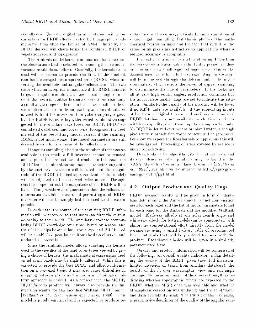
Global BRDF and Albedo Retrieval Over Land 183
sky albedos. Use of a digital terrain database will allowcorrection for BRDF e�ects created by topographic shad-ing some time after the launch of AM-1. Initially, theBRDF derived will characterize the combined BRDF ofvegetation/soil and topography.
The Ambrals model kernel combination that describesthe observations best is selected from among the �ve modelvariants available as follows. Generally, the kernels to beused will be chosen to provide the �t with the smallestroot band-averaged mean squared error (RMSE) when in-verting the available multiangular re ectances. The twocases where an exception is made are if the RMSE found islarge, or angular sampling coverage is bad enough to mis-trust the inversion, either because observations span onlya small angle range or their number is too small. In thesecases information from the supporting ancillary databasesis used to limit the inversion. If angular sampling is goodbut the RMSE found is high, the kernel combination sug-gested by the ancillary data (previous BRDF, BRDF ac-cumulated database, land cover type, topography) is usedinstead of the best-�tting model variant if the resultingRMSE is not much worse. The model parameters are stillderived from a full inversion of the re ectances.
If angular sampling is bad or the number of re ectancesavailable is too small, a full inversion cannot be trustedand gaps in the product would result. In this case, theBRDF kernel combinationand model parameters suggestedby the ancillary databases will be used, but the magni-tude of the BRDF (the isotropic constant of the model)will be adjusted to the observed re ectances. Throughthis the shape but not the magnitude of the BRDF will be�xed. This procedure also guarantees that the re ectanceinformation available in cases not permitting a full BRDFinversion will not be simply lost but used to the extentpossible.
In each case, the source of the resulting BRDF infor-mation will be recorded so that users can �lter the outputaccording to their needs. The ancillary database accumu-lating BRDF knowledge over time, keyed by season, andthe relationships between land cover type and BRDF usedwill be established post-launch from the data observed andupdated at intervals.
Since the Ambrals model allows adapting the kernelsused to the speci�cs of the land cover types viewed by giv-ing a choice of kernels, the mathematical expressions usedon adjacent pixels may be slightly di�erent. While this isexpected to provide the best BRDF and albedo informa-tion on a per-pixel basis, it may also cause di�culties inmapping between pixels and where a much simpler uni-form approach is desired. As a consequence, the MODISBRDF/albedo product will always also provide the fullinversion results for the modi�ed Walthall BRDF model[Walthall et al., 1985; Nilson and Kuusk, 1989]. Thismodel is purely empirical and is expected to produce re-
sults of reduced accuracy, particularly under conditions ofsparse angular sampling. But the simplicity of the math-ematical expression used and the fact that it will be thesame for all pixels are attractive to applications where areduced accuracy is acceptable.
Product generation rules are the following. If less than8 observations are available in the 16-day period, or theyare clustered in a small region of angle space, this will bedeemed insu�cient for a full inversion. Angular coveragewill be monitored through the determinant of the inver-sion matrix, which re ects the power of a given samplingto discriminate the model parameters. If the looks areall at very high zenith angles, production continues butthe appropriate quality ags are set to indicate this situ-ation. Similarly, the quality of the product will be lowerif no MISR data are available. If the supporting inputsof land cover, digital terrain and ancillary accumulatedBRDF database are not available, production continueswith lower quality, since these inputs are supportive only.No BRDF is derived over oceans or inland water, althoughpixels with subresolution water content will be processed.For snow we expect the Ross kernels to apply, but this willbe investigated. Processing of areas covered by sea ice isunder consideration.
Details about the algorithm, its theoretical basis, andits dependence on other products may be found in theNASA Algorithm Technical Basis Document [Strahler etal., 1995a], available on the internet at http://spso.gsfc.-nasa.gov/atbd/pg1.html.
4.2. Output Product and Quality Flags
BRDF inversion results will be given in form of identi-�ers determining the Ambrals model kernel combinationused for each pixel and the list of model parameters foundfor each band for the Ambrals and the modi�ed Walthallmodel. Black-sky albedo at any solar zenith angle andwhite-sky albedo for both models can be constructed withalmost no computational e�ort directly from the modelparameters using a small look-up table of precomputedkernel integrals that will be provided to users with theproduct. Broadband albedos will be given in a similarlyparameterized form.
Quality and product information will be comprised ofthe following: an overall quality indicator; a ag detail-ing the source of the BRDF given (new full inversion,limited inversion or taken from ancillary database); thequality of the �t over wavelengths; view and sun anglecoverage; the mean sun angle of the observations; ags in-dicating whether topographic e�ects are expected in theBRDF, whether MISR data was available and whetheratmospheric correction was updated; and the land/waterand data availability mask. The RMSE of the inversions,a quantitative descriptor of the quality of the angular sam-

184 Wanner et al.
pling found, and a parameter describing the relative con-tribution of surface and volume scattering to the scene arealso recorded.
In addition to this one-kilometer BRDF/albedo prod-uct, a product spatially degraded to a quarter-degree res-olution will be produced for direct use in climate models.This product will also carry information on the subgridvariability of albedo.
4.3. The Ambrals BRDF Inversion and
Modeling Tool
The production algorithm has been programmed to pro-vide maximum e�ciency through avoiding multiple evalu-ation of expressions shared by several kernels, and throughlook-up table approaches to kernel value retrieval and albedocalculations. One 16-day BRDF/albedo product at fullresolution and in all seven bands will have a total �le sizeof approximately 35 GByte. This size also applies to theBRDF knowledge database to be created. The process-ing power required to produce the 16-day product in real-time is currently estimated at about 300 million oatingpoint operations per second. Preparing the input data forBRDF/albedo processing requires additional resources.
A user working with the product will need to be able toreconstruct the BRDF from the parametrization providedby the MODIS BRDF/albedo product. For this, an al-gorithm is required that allows forward modeling of eachof the models used in the inversion. The Ambrals codewill be provided in a form that allows forward and inverseBRDF modeling of kernel-driven models, provides a selec-tion of science options, numerical BRDF integration, andpermits easy adding of new models. This code can also beused to degrade the product to coarser spatial resolutionsand derive the corresponding albedos. The Ambrals code,together with a user guide, is presently available from theauthors upon request for BRDF modeling work and prepa-ration of BRDF-dependent algorithms.
5. Validation
5.1. Validation Outline
Validation of the BRDF/albedo product will be performedin three respects. First, the semiempirical BRDF modelsneed to be validated for as many types of land cover as pos-sible to assure that they provide adequate mathematicaldescriptions of occurring BRDF shapes. This is done us-ing �eld-measured, laboratory-measured and numericallysimulated BRDFs.
Second, large-scale BRDF and albedo retrievals needto be demonstrated given the constraints of sampling, at-mospheric correction and temporal composition of dataoccurring in a remote sensing situation. This is done
using multiangular data from airborne sensors and fromAVHRR.
Third, the quality and accuracy of the product needto be monitored during post-launch product generation.This validation will be part of a MODIS-wide and EOS-wide validation and quality assurance e�ort based on towermeasurements, aircraft campaigns and intercomparisonswith the results obtained from other space-based sensors.
5.2. Model Validation
Basic model validation was carried out by applying theAmbrals BRDF model to multiangle re ectance data mea-sured in the �eld for a variety of land cover types. Herewe demonstrate this work by giving a few examples, se-lected to represent four distinct categories of land covertypes: forests; barren or sparsely vegetated lands; grassesand grasslike crops; and broadleaf crops. The data setsused include two soybean data sets observed by Ranson etal. [1985] using an Exotech Model 100 radiometer. Theyrepresent canopy coverages of 72 and 99 percent and solarzenith angle ranges from 20� to 49� and 31� to 61�, re-spectively. Inversion was carried out using all four bandsobserved, including the red and near-infrared. An aspenand a spruce forest data set were selected from measure-ments byDeering et al. [1995] using a PARABOLA instru-ment, and the red and near-infrared channel were used forinversions. The solar zenith angle range was 45� to 59�
and 36� to 59�, respectively. All other data were acquiredby Kimes [1983] and Kimes et al. [1985, 1986] at solarzenith angles ranging from 25� to 79�, varying from onedata set to another. The whole of the viewing hemispherewas sampled for all data sets.
Evaluations were carried out for the red and near-infrared (NIR) channels. Table 5 lists the data sets, givesthe model with the lowest root of the band-averaged squareddeviation between modeled and observed re ectances (RMSE),and the coe�cients of linear correlation between the mod-eled and observed re ectances in the red and in the NIRband. The RMSEs are found to be between 1.1 and 4.6percent, which is satisfactory, and the correlation coe�-cients commonly are larger than 0.8 or even 0.9. Theseresults are typical for those found for a number other datasets (including AVHRR, airborne POLDER, ASAS and�eld-measured data) using variants of the Ambrals modelused here [Privette and Vermote, 1995; Hu et al., 1996;White et al., 1996]. The corn data set has rather largeirregular variations in the observed re ectance, which ex-plains the low red band correlation coe�cient for this onedata set.
Figure 3 shows the correlation between observed andmodeled re ectances for one example from each of the fourland cover groups. Even though there are some deviations,the modeled re ectances generally follow the observed val-
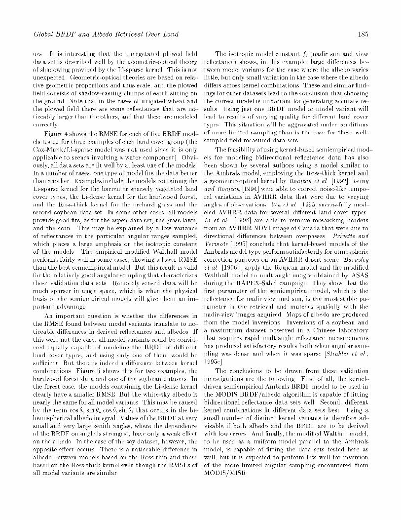
Global BRDF and Albedo Retrieval Over Land 185
ues. It is interesting that the unvegetated plowed �elddata set is described well by the geometric-optical theoryof shadowing provided by the Li-sparse kernel. This is notunexpected. Geometric-optical theories are based on rela-tive geometric proportions and thus scale, and the plowed�eld consists of shadow-casting clumps of earth sitting onthe ground. Note that in the cases of irrigated wheat andthe plowed �eld there are some re ectances that are no-ticeably larger than the others, and that these are modeledcorrectly.
Figure 4 shows the RMSE for each of �ve BRDF mod-els tested for three examples of each land cover group (theCox-Munk/Li-sparse model was not used since it is onlyapplicable to scenes involving a water component). Obvi-ously, all data sets are �t well by at least one of the models.In a number of cases, one type of model �ts the data betterthan another. Examples include the models containing theLi-sparse kernel for the barren or sparsely vegetated landcover types, the Li-dense kernel for the hardwood forest,and the Ross-thick kernel for the orchard grass and thesecond soybean data set. In some other cases, all modelsprovide good �ts, as for the aspen data set, the grass lawn,and the corn. This may be explained by a low varianceof re ectances in the particular angular ranges sampled,which places a large emphasis on the isotropic constantof the models. The empirical modi�ed Walthall modelperforms fairly well in some cases, showing a lower RMSEthan the best semiempirical model. But this result is validfor the relatively good angular sampling that characterizesthese validation data sets. Remotely sensed data will bemuch sparser in angle space, which is when the physicalbasis of the semiempirical models will give them an im-portant advantage.
An important question is whether the di�erences inthe RMSE found between model variants translate to no-ticeable di�erences in derived re ectances and albedos. Ifthis were not the case, all model variants could be consid-ered equally capable of modeling the BRDF of di�erentland cover types, and using only one of them would besu�cient. But there is indeed a di�erence between kernelcombinations. Figure 5 shows this for two examples, thehardwood forest data and one of the soybean datasets. Inthe forest case, the models containing the Li-dense kernelclearly have a smaller RMSE. But the white-sky albedo isnearly the same for all model variants. This may be causedby the term cos �v sin �v cos �i sin �i that occurs in the bi-hemispherical albedo integral. Values of the BRDF at verysmall and very large zenith angles, where the dependenceof the BRDF on angle is strongest, have only a weak e�ecton the albedo. In the case of the soy dataset, however, theopposite e�ect occurs. There is a noticeable di�erence inalbedo between models based on the Ross-thin and thosebased on the Ross-thick kernel even though the RMSEs ofall model variants are similar.
The isotropic model constant fi (nadir sun and viewre ectance) shows, in this example, large di�erences be-tween model variants for the case where the albedo varieslittle, but only small variation in the case where the albedodi�ers across kernel combinations. These and similar �nd-ings for other datasets lead to the conclusion that choosingthe correct model is important for generating accurate re-sults. Using just one BRDF model or model variant willlead to results of varying quality for di�erent land covertypes. This situation will be aggravated under conditionsof more limited sampling than is the case for these well-sampled �eld-measured data sets.
The feasibility of using kernel-based semiempiricalmod-els for modeling bidirectional re ectance data has alsobeen shown by several authors using a model similar tothe Ambrals model, employing the Ross-thick kernel anda geometric-optical kernel by Roujean et al. [1992]. Leroyand Roujean [1994] were able to correct noise-like tempo-ral variations in AVHRR data that were due to varyingangles of observations. Wu et al. [1995] successfully mod-eled AVHRR data for several di�erent land cover types.Li et al. [1996] are able to remove mosaicking bordersfrom an AVHRR NDVI image of Canada that were due todirectional di�erences between overpasses. Privette andVermote [1995] conclude that kernel-based models of theAmbrals model type perform satisfactorily for atmosphericcorrection purposes on an AVHRR desert scene. Barnsleyet al. [1996b] apply the Roujean model and the modi�edWalthall model to multiangle images obtained by ASASduring the HAPEX-Sahel campaign. They show that the�rst parameter of the semiempirical model, which is there ectance for nadir view and sun, is the most stable pa-rameter in the retrieval and matches spatially with thenadir-view images acquired. Maps of albedo are producedfrom the model inversions. Inversions of a soybean anda nasturtium dataset observed in a Chinese laboratorythat acquires rapid multiangle re ectance measurementshas produced satisfactory results both when angular sam-pling was dense and when it was sparse [Strahler et al.,1995c].
The conclusions to be drawn from these validationinvestigations are the following. First of all, the kernel-driven semiempirical Ambrals BRDF model to be used inthe MODIS BRDF/albedo algorithm is capable of �ttingbidirectional re ectance data sets well. Second, di�erentkernel combinations �t di�erent data sets best. Using asmall number of distinct kernel variants is therefore ad-visable if both albedo and the BRDF are to be derivedwith low errors. And �nally, the modi�ed Walthall model,to be used as a uniform model parallel to the Ambralsmodel, is capable of �tting the data sets tested here aswell, but it is expected to perform less well for inversionof the more limited angular sampling encountered fromMODIS/MISR.
186 Wanner et al.
Additional �eld-measured BRDF data sets are expectedto be available for continued model validation. The BRDFlaboratory in Changchun, China, [Strahler et al., 1995c;Liang et al., 1996] will provide additional BRDF measure-ments in the future. Data acquired during the BOREAScampaigns are beginning to be available, such as the PARA-BOLA data sets by Deering et al. [1995], two of whichwere used in this paper. Arti�cial data sets have beencreated by So�er et al. [1995] using model trees in a labo-ratory, and by Lewis and Muller [1992] using Monte Carloray-tracing. BRDF data sets generated numerically forseveral di�erent biome types from a 3D-radiative transfercode by Myneni et al. [1992] are being employed for adetailed study of model properties that will be reportedelsewhere.
5.3. Relationship of BRDF to Land Cover
In Figure 4, there is an indication of distinctive patternscharacterizing each land cover type group. In the case ofthe hardwood forest, clearly the two models involving theLi-dense kernel are much favored over those involving theLi-sparse kernel. This corresponds to the fact that theforest observed was indeed dense in nature. There is littledi�erence between the model using the Ross-thick kerneland the model using the Ross-thin kernel. This may beexplained by the fact that scattering is dominated by geo-metric optics, leading to a small weight given to the volumescattering kernel. It does not matter which one is chosen.The case is less clear for the pine and the aspen data sets,but the aspen does show a slight improvement of �ts ifthe Ross-thick kernel is used. Although it might well beexpected from the scene type, this data set lacks a distincthotspot, perhaps due to instrument characteristics.
All the examples given for barren or sparsely vege-tated covers show a distinct preference for the Li-sparsekernel, which is driven by shadowing. The plowed �eldconsisted of clumps of earth on the ground, leading tostrong surface scattering e�ects. The annual grass dataset was acquired at a site with less than 5 percent of veg-etation cover, where 40 percent of the surface was coveredby stones and pebbles [Kimes and Sellers, 1985]. Thesteppe grass site had clumps of grass, and the total coverwas 18 percent. Obviously, the structured surface of theseland covers is best represented by strong shadow-drivengeometric-optical scattering.
Two of the three data sets given for dense grasses andgrasslike crops show a preference for models containingthe Ross-thick kernel, as might be expected for dense hor-izontally layered canopies that show little shadowing. Inthe broadleaf crops group, two of the three examples givenare modeled well by all models. They lack angular varia-tion in the angle intervals sampled, resulting in a strongisotropic contribution to overall �tting that renders the
contributions from the respective kernels less important.One set, however, shows the in uence of both shadowingand volume scattering in being modeled best by the Ross-thick/Li-dense model.
We think that there is an indication in this data thatwhere mutual shadowing of crowns plays a role, as inmost forests, models containing the Li-dense kernel will bechosen, whereas in scenes where shadows are dominant,models using the Li-sparse kernel are preferred. Thesescenes would then be sparse forests or brushlands, androck-strewn deserts, rough (plowed) terrain or clumpedvegetation, respectively. When the Ross-thick kernel ischosen over the Ross-thin kernel, or all models performwell, a dense layered canopy with no individual crowns isobserved. The Ross-thin kernel is expected to be applica-ble to scenes with a thin but horizontally continuous layerof leaves over a rather solid background, which can be theground or dense underlying vegetation.
Table 6 summarizes these correspondences in a tenta-tive list of land covers likely to be associated with mod-els containing speci�c kernels. Whether the relationshipsspeculated upon here hold with any consistency, and whetherthe di�erences are distinct enough to allow reliable infer-ence of surface structural properties, remains to be seenwhen much more extensive data sets than are now avail-able can be studied. But the fact that surface structuredetermines the angular dependence of the re ectance, as isknown from physical re ectance forward modeling, shouldmake a retrieval of at least general structural informa-tion of the type discussed here possible [Goel, 1989; Pintyand Verstraete, 1991]. If the classes obtained from suchan analysis are not congruent with the classes derivedfrom spectral land cover classi�cations, the combinationof directional and spectral information should allow formore accuracy in land cover classi�cation. An example isthe distinction between dense and sparse forests, or be-tween dense brush and sparse forest, which may have sim-ilar spectral properties but distinct bidirectional charac-teristics. A study by Barnsley et al. [1996a] shows thatwhile the spectral information content of a scene of arablefarmland obtained with the airborne multispectral scannerDaedalus is greater than the directional information con-tent, the multiangle properties of the data neverthelessprovide an important means of distinguishing between theoccurring land cover types. For this reason, the MODISland cover product will make use of BRDF-derived infor-mation where feasible [Strahler at al., 1995b].
5.4. Pre-Launch Product Prototyping
Several projects are close to completion that apply theAmbrals BRDF model to AVHRR data over large regions,demonstrating and testing the MODIS algorithm. It is be-yond the scope of this paper to report this work in detail.

Global BRDF and Albedo Retrieval Over Land 187
A study led by d'Entremont [d'Entremont et al., 1995,1996] is targeted at inversions of AVHRR multiangle im-agery for the whole of New England. Maps of albedo andkernel combinations chosen have been derived. A projectconducted by Lewis includes large-area AVHRR data in-versions for di�erent times of the year for the Sahel regionof Africa. A similar investigation, led by X. Li, is underway for a large area surrounding the site of Three Gorgesdam project on the Yangtse river in China. These sci-enti�c studies, which also serve to prototype the MODISBRDF/albedo product, demonstrate the feasibility of theapproach and have been successful in generating BRDFand albedo images of large areas. Validation of the re-sults obtained is the next step. In the Sahel region, forexample, both ground-measured and airborne sensor mul-tiangular data have also been evaluated for comparison.
Other sources of large-area data that will be used whenthey become available are data from the POLDER instru-ment, launched in August 1996, and the SPOT-VEGE-TATION sensor, also to be launched before the AM-1platform. These data sets, observed from space, will becomplemented by more limited datasets acquired from air-borne sensors. Here, several campaigns have been car-ried out and will be carried out in the future with theASAS, the MODIS airborne simulator (MAS), the com-pact airborne spectrographic imager (CASI) and the air-borne POLDER sensors over a variety of sites. Work onprocessing these data is under way. Semiempirical modelswill be and are being applied to these data sets to opti-mize the algorithm for deriving BRDF and albedo fromMODIS/MISR. AirMISR is a MISR-like instrument thatwill be very relevant to BRDF studies once it is operationalin 1997.
5.5. Post-Launch Product Validation
In the post-launch phase, a coordinated e�ort for validat-ing the radiometric products of MODIS and EOS as awhole will be undertaken. Validation of BRDF and albedois tied into validation of calibration, atmospheric correc-tion, and several higher-order products. This e�ort is cur-rently being developed in the EOS project.
A number of tower sites will be equipped with ra-diometers monitoring upwelling and downwelling radianceson a continuous basis. At a minimum, these sensors willrecord broadband hemispherical uxes. Spectral measure-ments will be made whereever possible. A selected num-ber of sites will also feature directional measurements. Thestatus of the land cover around the towers and atmosphericproperties over the towers will be measured simultane-ously. Tower sites will be chosen to represent major landcover types. One problem with many current sites observ-ing aerosols, for example, is that little attention is givento the upward uxes coming back from the surface (e.g.,
rooftop instruments will not do).
The observations obtained at a tower site will be scaledto the footprint size of the space-based sensor through oc-casional aircraft over ights that relate site properties tosurrounding areas. Additionally, sites will be chosen tobe homogeneous in land cover type. Scaling may also beinferred from using data from sensors with di�erent reso-lutions.
An important part of post-launch product monitoringwill also be cross-comparing the MODIS BRDF/albedoproduct with the corresponding MISR surface product andthe POLDER BRDF and albedo product. Use of datacomparable data from meteorological satellites for valida-tion purposes will also be investigated.
6. Conclusions
Surface re ectance is a key quantity in optical remote sens-ing. A multitude of derived parameters and estimates arebased on surface re ectance, for example land cover clas-si�cations, snow and ice maps, and vegetation state pa-rameters. However, since the re ectance of the land sur-face is anisotropic in nature, retrieval of the bidirectionalre ectance distribution function is essential for an exactinterpretation of the data, and for characterizing averagere ectance in form of albedo measures. In addition, BRDFand albedo are required for accurate computations of ra-diative transport in the atmosphere, providing the direc-tional characteristics and the magnitude of scattering atthe lower boundary. This is of importance in atmosphericcorrection and in the radiation transfer schemes of climateand weather models.
The MODIS BRDF/albedo product will provide thisinformation to a wide variety of users as part of the EOS-MODIS standard product catalogue. The expected usescomprise correction of images for directional e�ects; stan-dardizing images to common viewing and illumination ge-ometries; deriving vegetation indexes free of directionale�ects; providing lower boundaries for atmospheric cor-rection and radiation budget investigations; retrieving pre-cise measures of land surface albedo; inferring land surfacestructural characteristics, especially of vegetation and to-pography; and as an input to land cover classi�cation. Apossible future application is in cloud detection.
The MODIS BRDF/albedo product will employ theAmbrals kernel-based semiempirical BRDF model, mak-ing use of a total of �ve di�erent available kernel functions,and the modi�ed Walthall model for modeling the multi-angle data. These models have been shown to �t a varietyof observed multiangular data sets well. Besides possess-ing bene�cial computational qualities, such as analyticalinversion, direct spatial scaling and generic accommoda-tion of mixed pixels, their physical basis allows for credible
188 Wanner et al.
extrapolation of the BRDF to angles not covered by theobservations. The BRDFs found will be integrated to pro-vide integral measures of albedo that do not depend onatmospheric state.
The combination of these activities, it is hoped, willcontribute to the goal of EOS, to further the understand-ing of the earth system in a time of potentially large changesinduced by human activity. The production of a routineglobal BRDF and albedo product will lead to an increasedunderstanding of the role that directional anisotropy inthe re ectance of the earth's surface plays in the globalenergy system.
Acknowledgments. We would like to thank Jor-dan Borak for generating the data for the narrowband-to-broadband conversions shown in Table 3, Baojin Zhang forwork on model inversion accuracy under varying angularsampling, and Jim Tallent for taking the beta-version ofthe Ambrals code to version 1. This work was supportedin the US by NASA under NAS5-31369, and in the UKby NERC under the TIGER-SVATS programme and theEuropean Union under the 3rd Famework Human Capitaland Mobility Programme.
Barnsley, M. J., A. H. Strahler, K. P. Morris, and J.-P. Muller, Sampling the surface bidirectional re- ectance distribution function (BRDF): Evaluationof current and future satellite sensors, Remote Sens.Rev. 8, 271{311, 1994.
Barnsley, M. J., D. Allison, and P. Lewis, On the informa-tion content of multiple-view-angle (MVA) images,Int. J. Remote Sens., in press, 1996a.
Barnsley, M. J., P. Lewis, M. Sutherland, and J.-P.Muller,Estimating land surface albedo in the HAPEX-Sahelsouthern super-site: Inversion of two BRDF modelsagainst multiple angle ASAS images, J. Hydrol., inpress, 1996b.
Brest, C. L., and S. N. Goward, Deriving surface albedomeasurements from narrow band satellite data, Int.J. Remote Sens., 8, 351{367, 1987.
Cihlar, J., D. Manak, and N. Voisin, AVHRR bidirec-tional re ectance e�ects and compositing, RemoteSens. Env., 48, 77{88, 1994.
Cox, C., and W. H. Munk, The measurement of theroughness of the sea surface from photographs of thesun glitter, J. Opt. Soc. Am., 44, 838{850, 1954.
Deering, D. W., S. P. Ahmad, T. F. Eck, and B. P.Banerjee, Temporal attributes of the bidirectionalre ectance for three boreal forest canopies, Proc.Int. Geosci. Remote Sens. Symp. 95, 1239{1241,1995.
Deschamps, P. Y., F. M. Breon, M. Leroy, A. Podaire, A.Bricaud, J. C. Buriez, and G. Seze, The POLDERmission: Instrument characteristics and scienti�cobjectives, IEEE Trans. Geosci. Remote Sens., 32,598{615, 1994.
Dickinson, R. E., Land surface processes and climate-surface albedos and energy, Adv. Geophys., 25, 305{353, 1983.
DiGirolamo, L., and R. Davies, A band-di�erence angu-lar signature technique for cirrus cloud detection,IEEE Trans. Geosci. Remote Sens., 32, 890{896,1994.
Diner, D., C. J. Bruegge, J. V. Martonchik, G. W. Both-well, E. D. Danielson, V. G. Ford, L. E. Hovland,K. L. Jones, and M. L. White, A multi-angle im-age spectroradiometer for terrestrial remote sensingwith the Earth Observing System, Int. J. Imag. Sys.Tech., 3, 92{107, 1991.
d'Entremont, R. P., C. B. Schaaf, and A. H. Strahler,Cloud detection and land surface albedos using vis-ible and near-infrared bidirectional re ectance dis-tribution models, Proc. SPIE Symp. Sat. RemoteSens., 2586, 1995.
d'Entremont, R. P., C. B. Schaaf, and A. H. Strahler,Using infrared cloud clearing techniques in the es-timation of AVHRR-based bidirectional re ectancedistributions functions, Proc. 8th Conf. Sat. Met.Oceanog., 334{338, 1996.
Goel, N. S., Inversion of canopy re ectance models for es-timation of biophysical parameters from re ectancedata, in Theory and Applications of Optical RemoteSensing, pp. 205{251, J. Wiley & Sons, New York,1989.
Gutman, G., Normalization of multi-annual global AVHRRre ectance data over land surfaces to common sun-target-sensor geometry,Adv. Space Res., 14(1), 121{124, 1994.
Henderson-Sellers, A., and M. F. Wilson, Surface albedofor climate modeling, Rev. Geophys. Space Sci., 21,1743{1778, 1983.
Hu, B., W. Wanner, X. Li, and A. Strahler, Validationof kernel-driven semiempirical BRDF models for ap-plication to MODIS-MISR data, Proc. Int. Geosci.Remote Sens. Symp. 96, 1669{1671, 1996.
Kaufman, Y. J., The atmospheric e�ect on remote sens-ing and its correction, in Theory and Applicationsof Optical Remote Sensing, pp. 336{428, J. Wiley &Sons, New York, 1989.
Global BRDF and Albedo Retrieval Over Land 189
Kimes, D. S., Dynamics of directional re ectance fac-tor distribution for vegetation canopies, Appl. Opt.,22(9), 1364{1372, 1983.
Kimes, D. S., W. W. Newcomb, C. J. Tucker, I. S. Zonn-eveldt, W. van Wijngaarden, J. de Leeuw, and G. F.Epema, Directional re ectance factor distributionsfor cover types of Northern Africa, Remote Sens.Env., 18, 1{19, 1985.
Kimes, D. S., W. W. Newcomb, R. F. Nelson, and J.B. Schutt, Directional re ectance distributions of ahardwood and a pine forest canopy, IEEE Trans.Geosci. Remote Sens., 24, 281{293, 1986.
Kimes, D. S., and P. J. Sellers, Inferring hemisphericalre ectance of the earth's surface for global energybudgets from remotely sensed nadir or directionalradiance values, Remote Sens. Env., 18, 205{223,1985.
Kriebel, K. T., Measured spectral bidirectional re ectionproperties of four vegetated surfaces, Appl. Optics,17(2), 253{259, 1978.
Kustas, W. P., R. D. Jackson, and G. Asrar, Estimatingsurface energy-balance components from remotelysensed data, in Theory and Applications of OpticalRemote Sensing, pp. 604{627, J. Wiley & Sons, NewYork, 1989.
Lee, T. Y., and Y. J. Kaufman, Non-Lambertian e�ectsin remote sensing of surface re ectance and vegeta-tion index, IEEE Trans. Geosci. Remote Sens., 24,699{708, 1986.
Leroy, M., and J.-L. Roujean, Sun and view angle correc-tions on re ectances derived from NOAA/AVHRRdata, IEEE Trans. Geosci. Remote Sens., 32, 684{697, 1994.
Leroy, M., J. L. Deuze, F. M. Breon, O. Hautecoeur,M. Herman, J. C. Buriez, D. Tanre, S. Bou�es,P. Chazette, and J.-L. Roujean, Retrieval of at-mospheric properties and surface bidirectional re- ectances over land fromPOLDER/ADEOS, J. Geo-phys. Res., this issue, 1996.
Lewis, P., The utility of kernel-driven BRDF models inglobal BRDF and albedo studies, Proc. Int. Geosci.Remote Sens. Symp. 95, 1186{1187, 1995.
Lewis, P., and M. J. Barnsley, In uence of sky radiancedistribution on various formulations of earth surfacealbedo, Proc. 6th Int. Symp. Phys. Meas. Sign. Re-mote Sens., 707{715, 1994.
Lewis, P., and J.-P. Muller, The advanced radiometricray-tracer: ARARAT for plant canopy re ectancesimulation,Proc. 29th Conf. Int. Soc. Photogramm.Remote Sens., 26{34, 1992.
Li, X., and A. H. Strahler, Geometric-optical bidirec-tional re ectance modeling of the discrete crownvegetation canopy: e�ect of crown shape and mu-tual shadowing, IEEE Trans. Geosci. Remote Sens.,30, 276{292, 1992.
Li, Z., and L. Garand, Estimation of surface albedo fromspace: A parametrization for global application, J.Geophys. Res., 99, 8335{8350, 1994.
Li, Z., X. Zheng, L. Moreau, and H. Ly, Detection andcorrection of bidirectional e�ects in AVHRR mea-surements over northern regions, IEEE Trans. Geosci.Remote Sens., in press, 1996.
Liang, S., A. H. Strahler, Q. Zhu, and X. Jin, Com-parisons of radiative transfer models of vegetationcanopies and laboratory measurements, IEEE Trans.Geosci. Remote Sens., in press, 1996.
Moody, A., and A. H. Strahler, Characteristics of com-posited AVHRR data and problems in their classi-�cation, Int. J. Remote Sens., 15, 3473{3491, 1994.
Myneni, R. B., Asrar, G., and F. G. Hall, A three-dimensionalradiative transfer method for optical remote sensingof vegetated land surfaces, Remote Sens. Env., 41,105{121, 1992.
Nilson, T., and A. Kuusk, A re ectance model for the ho-mogeneous plant canopy and its inversion, RemoteSens. Env., 27, 157{167, 1989.
Nicodemus, F. E., J. C. Richmond, J. J. Hsia, I. W.Ginsberg, and T. Limperis, Geometrical considera-tions and nomenclature for re ectance, Nat. BureauStand. Report, NBS MN-160, 52 pp., 1977.
Pinty, B., and M. M. Verstraete, Extracting informationon surface properties from bidirectional re ectancemeasurements, J. Geophys. Res, 96, 2865{2874, 1991.
Pinty, B., M. M. Verstraete, and R. E. Dickinson, A phys-ical model for predicting bidirectional re ectanceover bare soil,Remote Sens. Env., 27, 273{288, 1989.
Privette, J. L., and E. F. Vermote, Fitting remote sens-ing data with linear bidirectional re ectance models,Proc. SPIE Symp. Sat. Remote Sens., 2586, 172{179, 1995.
Rahman, H., B. Pinty, and M. M. Verstraete, Coupledsurface-atmosphere re ectance (CSAR) model, 2,Semiempirical surface model usable with NOAA ad-vanced very high resolution radiometer data, J. Geo-phys. Res., 98, 20,791{20,801, 1993.
Ranson, K. J., L. L. Biehl, and M. E. Bauter, Varia-tion in spectral response of soybeans with respectto illumination, view and canopy geometry, Int. J.Remote Sens., 6, 1827{1842, 1985.
190 Wanner et al.
Ranson, K. J., J. R. Irons, and C. S. T. Daughtry, Surfacealbedo from bidirectional re ectance, Remote Sens.Env., 35, 201{211, 1991.
Ross, J. K., The Radiation Regime and Architecture ofPlant Stands, 392 pp., Dr. W. Junk Publishers, TheHague, 1981.
Roujean, J. L., M. Leroy, and P. Y. Deschamps, A bidi-rectional re ectance model of the earth's surface forthe correction of remote sensing data, J. Geophys.Res., 97, 20,455{20,468, 1992.
Roujean, J.-L., D. Tanre, F.-M. Breon, and J.-L. Deuze,An improved land surface parameters retrieval fromPOLDER bidirectional measurements during HAPEX-Sahel, Proc. Int. Geosci. Remote Sens. Symp. 95,1293{1295, 1995.
Running, S. W., E. R. Hunt, R. Nemani, and J. Glassy,MODIS leaf area index and fraction photosynthet-ically active radiation: Algorithm theoretical basisdocument, NASA EOS-MODIS Doc., 21 pp., 1995.
Running, S. W., C. O. Justice, V. Salomonson, D. Hall,J. Barker, Y. J. Kaufman, A. H. Strahler, A. R.Huete, J.-P. Muller, V. Vanderbilt, Z. M. Wan, P.Teillet, and D. Carneggie, Terrestrial remote sensingscience and algorithms planned for EOS/MODIS,Int. J. Remote Sens., 15, 3587{3620, 1994.
Sellers, P. J., Remote sensing of the land surface for stud-ies of global change, NASA/GSFC Int. Sat. LandSurf. Clim. Proj. Report, 1993.
Sellers, P. J., C. J. Tucker, G. J. Collatz, S. O. Los, C. O.Justice, D. A. Dazlich, and D. A. Randall, A global 1degree by 1 degree NDVI data set for climate stud-ies, Part 2, The generation of global �elds of ter-restrial biophysical parameters from NDVI, Int. J.Remote Sens., 15, 3519{3545, 1994.
So�er, R. J., J. R. Miller, W. Wanner, and A. Strahler,Winter boreal forest canopy BRF results: Com-parisons between airborne data, laboratory simula-tions and geometrical-optical model data, Proc. Int.Geosci. Remote Sens. Symp. 95, 800{802, 1995.
Starks, P. J., J. M. Norman, B. L. Blad, E. A. Walter-Shea, and C. L. Walthall, Estimation of shortwavehemispherical re ectance (albedo) from bidirection-ally re ected radiance data, Remote Sens. Env., 38,123{134, 1991.
Strahler, A. H., Vegetation canopy re ectance modeling{ recent developments and remote sensing perspec-tives, Proc. 6th Int. Symp. Phys. Meas. Sign., 593{600, 1994.
Strahler, A. H. X. Li, S. Liang, J.-P. Muller, M. J. Barns-ley, and P. Lewis, MODIS BRDF/albedo product:Algorithm technical basis document, NASA EOS-MODIS Doc., version 2.1, 55 pp., 1994.
Strahler, A. H., M. J. Barnsley, R. d'Entremont, B. Hu,P. Lewis, X. Li, J.-P. Muller, C. B. Schaaf, W. Wan-ner, and B. Zhang, MODIS BRDF/albedo product:Algorithm theoretical basis document, NASA EOS-MODIS Doc. and update, version 3.2, 65 pp., 1995a.
Strahler, A. H., A. Moody, E. Lambin, A. Huete, C. Jus-tice, J.-P. Muller, S. Running, V. Salomonson, V.Vanderbilt, and Z. Wan, MODIS land cover prod-uct: Algorithm technical basis document, NASAEOS MODIS Doc., version 3.1, 42 pp., 1995b.
Strahler, A. H., W. Wanner, Q. Zhu, and X. Jin, Bidirec-tional re ectance modeling of data from vegetationobtained in the Changchun Solar Simulation Labo-ratory, Proc. Int. Geosci. Remote Sens. Symp. 95,1965{1967, 1995c.
Vermote, E. F., L. A. Remer, C. O. Justice, Y. J. Kauf-man, and D. Tanre, MODIS atmospheric correctionalgorithm: spectral re ectances, Algorithm techni-cal basis document, NASA EOS MODIS Doc., ver-sion 2.0, 42 pp. 1995.
Vermote, E. F., N. El Saleous, C. O. Justice, Y. F. Kauf-man, J. L. Privette, L. Remer, J. C. Roger, and D.Tanre, Atmospheric correction of visible to middleinfrared EOS-MODIS data over the land surface:background, operational algorithm and validation,J. Geophys. Res., this issue, 1996.
Vermote, E. F., D. Tanre, J. L. Deuze, M. Herman, andJ. J. Morcrette, Second simulation of the satellitesignal in the solar spectrum: an overview, IEEETrans. Geosci. Remote Sens., in press, 1996.
Walthall, C. L., J. M. Norman, J. M. Welles, G. Camp-bell, and B. L. Blad, Simple equation to approx-imate the bidirectional re ectance from vegetationcanopies and bare soil surfaces, Appl. Opt., 24, 383{387, 1985.
Wanner, W., X. Li, and A. H. Strahler, On the deriva-tion of kernels for kernel-driven models of bidirec-tional re ectance, J. Geophys. Res., 100, 21077{21090, 1995a.
Wanner, W., A. H. Strahler, J.-P. Muller, M. Barnsley,P. Lewis, X. Li, and C. L. Barker Schaaf, Globalmapping of bidirectional re ectance and albedo forthe EOS MODIS project: the algorithm and theproduct, Proc. Int. Geosci. Remote Sens. Symp. 95,525{529, 1995b.
Global BRDF and Albedo Retrieval Over Land 191
Wanner, W., P. Lewis, and J.-L. Roujean, The in uenceof directional sampling on bidirectional re ectanceand albedo retrieval using kernel-driven models,Proc.Int. Geosci. Remote Sens. Symp. 96, 1408{1410,1996.
Whittaker, E., and G. Robinson, The Calculus of Obser-vations, Blachie and Son, Glasgow, 397 pp., 1960.
White, H. P., R. So�er, J. R. Miller, and W. Wanner,Semiempirical modeling of bidirectional re ectanceutilizing the MODIS BRDF/albedo algorithmmod-els Proc. Int. Geosci. Remote Sens. Symp. 96, 1411{1413, 1996.
Wu, A., Z. Li, and J. Cihlar, E�ects of land cover typeand greenness on advanced very high resolution ra-diometer bidirectional re ectances: Analysis and re-moval, J. Geophys. Res., 100, 9179{9192, 1995.
Wylie, D. P., and W. P. Menzel, Two years of cloud coverstatistics using VAS, J. Climate, 2, 380{392, 1989.
Wylie, D. P., W. P. Menzel, H. M. Woolf, and K. I. Stra-bala, Four years of global cirrus cloud statistics us-ing HIRS, J. Climate, 7, 1972{1986, 1994.
Zhang, Y.-C., W. B. Rossow, and A. A. Lacis, Calcu-lation of surface and top of atmosphere radiative uxes from physical quantities based on ISCCP datasets, 1. Method and sensitivity to input data set un-certainties, J. Geophys. Res., 100, 1149{1165, 1995.
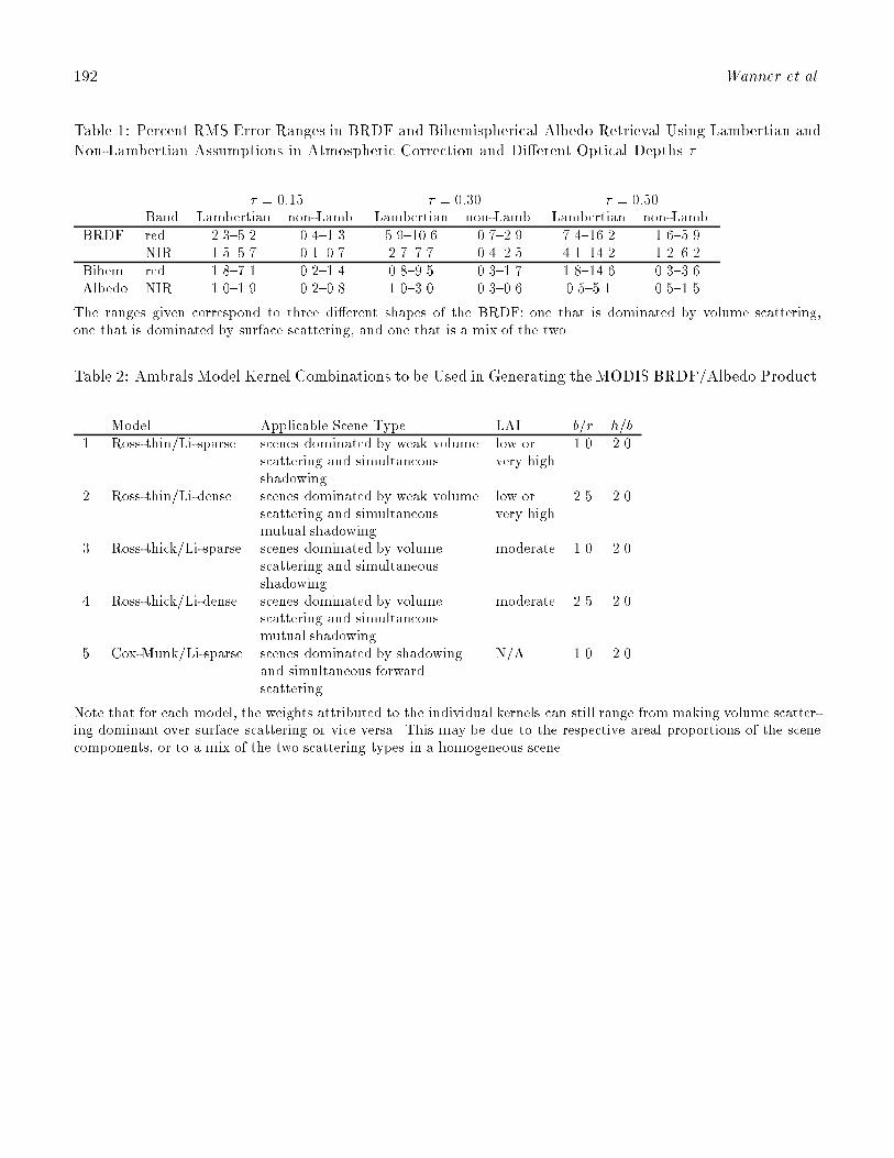
192 Wanner et al.
Table 1: Percent RMS Error Ranges in BRDF and Bihemispherical Albedo Retrieval Using Lambertian andNon-Lambertian Assumptions in Atmospheric Correction and Di�erent Optical Depths � .
� = 0:15 � = 0:30 � = 0:50Band Lambertian non-Lamb. Lambertian non-Lamb. Lambertian non-Lamb.
BRDF red 2.3{5.2 0.4{1.3 5.9{10.6 0.7{2.9 7.4{16.2 1.6{5.9NIR 1.5{5.7 0.1{0.7 2.7{7.7 0.4{2.5 4.1{14.2 1.2{6.2
Bihem. red 1.8{7.1 0.2{1.4 0.8{9.5 0.3{1.7 1.8{14.6 0.3{3.6Albedo NIR 1.0{1.9 0.2{0.8 1.0{3.0 0.3{0.6 0.5{5.1 0.5{1.5
The ranges given correspond to three di�erent shapes of the BRDF: one that is dominated by volume scattering,one that is dominated by surface scattering, and one that is a mix of the two.
Table 2: Ambrals Model Kernel Combinations to be Used in Generating the MODIS BRDF/Albedo Product.
Model Applicable Scene Type LAI b=r h=b
1. Ross-thin/Li-sparse scenes dominated by weak volume low or 1.0 2.0scattering and simultaneous very highshadowing
2. Ross-thin/Li-dense scenes dominated by weak volume low or 2.5 2.0scattering and simultaneous very highmutual shadowing
3. Ross-thick/Li-sparse scenes dominated by volume moderate 1.0 2.0scattering and simultaneousshadowing
4. Ross-thick/Li-dense scenes dominated by volume moderate 2.5 2.0scattering and simultaneousmutual shadowing
5. Cox-Munk/Li-sparse scenes dominated by shadowing N/A 1.0 2.0and simultaneous forwardscattering
Note that for each model, the weights attributed to the individual kernels can still range from making volume scatter-ing dominant over surface scattering or vice versa. This may be due to the respective areal proportions of the scenecomponents, or to a mix of the two scattering types in a homogeneous scene.
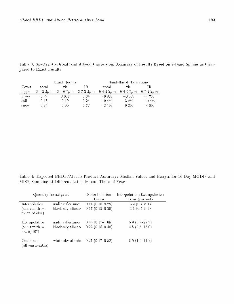
Global BRDF and Albedo Retrieval Over Land 193
Table 3: Spectral-to-Broadband Albedo Conversion: Accuracy of Results Based on 7-Band Splines as Com-pared to Exact Results.
Exact Results Band-Based, DeviationsCover total vis IR total vis IRType 0.4-2.2�m 0.4-0.7�m 0.7-2.2�m 0.4-2.2�m 0.4-0.7�m 0.7-2.2�mgrass 0.22 0.058 0.34 -0.9% +0.5% -1.2%soil 0.18 0.10 0.24 -0.4% -3.2% +0.4%snow 0.84 0.99 0.72 -2.1% -0.2% -4.0%
Table 4: Expected BRDF/Albedo Product Accuracy: Median Values and Ranges for 16-Day MODIS andMISR Sampling at Di�erent Latitudes and Times of Year.
Quantity Investigated Noise In ation Interpolation/ExtrapolationFactor Error (percent)
Interpolation nadir re ectance 0.21 (0.18{0.28) 3.3 (0.7{8.1)(sun zenith = black-sky albedo 0.17 (0.15{0.20) 3.1 (0.5{9.6)mean of obs.)
Extrapolation nadir re ectance 0.45 (0.17{1.08) 5.9 (0.8{28.7)(sun zenith = black-sky albedo 0.23 (0.18{0.49) 4.8 (0.8{16.0)nadir/10�)
Combined white-sky albedo 0.31 (0.17{0.82) 6.0 (1.4{14.2)(all sun zeniths)

194 Wanner et al.
Table 5: Sample Ambrals Model Fit Accuracies Using Field-Measured BRDFs of Several Di�erent LandCover Types in the Red and NIR Bands.
Cover Type Source Best-�t Kernels RMSE (%) r (red,%) r (NIR,%)
Needleleaf and Broadleaf ForestsDense hardwood forest Kimes Ross-thick/Li-dense 3.0 0.90 0.89Dense pine forest Kimes Ross-thin/Li-dense 4.1 0.78 0.72Aspen forest Deering Ross-thick/Li-sparse 2.5 0.92 0.88Spruce forest Deering Ross-thick/Li-sparse 1.1 0.95 0.94
Barren, Soil, Sparse VegetationPlowed Field Kimes Ross-thick/Li-sparse 1.6 0.98 0.98Annual grass (cover. <5%) Kimes Ross-thick/Li-sparse 2.3 0.95 0.88Steppe grass (coverage18%)
Kimes Ross-thick/Li-sparse 2.4 0.89 0.92
Grasses, Grasslike CropsGrass lawn Kimes Ross-thin/Li-dense 4.6 0.72 0.84Irrigated wheat Kimes Ross-thick 3.7 0.91 0.92Orchard grass Kimes Ross-thick/Li-sparse 3.1 0.84 0.91
Broadleaf CropsSoybeans (coverage 72%) Ranson Ross-thick/Li-sparse 1.7 0.75 0.89Soybeans (coverage 99%) Ranson Ross-thick 1.1 0.91 0.93Soybeans (coverage 90%) Kimes Ross-thick/Li-sparse 4.3 0.78 0.81Corn (coverage 25%) Kimes Ross-thin/Li-dense 2.8 0.47 0.75
Sources: Deering = Deering et al. [1995]; Ranson = Ranson et al. [1985]; Kimes = Kimes [1983], Kimes et al.[1985, 1986].

Global BRDF and Albedo Retrieval Over Land 195
Table 6: Expected Relationship Matrix of Ambrals Kernels to Land Cover Types.
Models composed ofthe following twokernels (left+down):
Li-sparse kernel:sparse distinctcrowns/objects
Li-dense kernel:dense distinctcrowns/objects
low weight forLi-kernels:no distinct crowns
low weight forRoss-kernels: noleaf-level scattering
plowed �elds,rock-strewn lands,rugged topography;mosaics of these withsparse woodlands
dense buildings Lambertian surface
Ross-thin kernel:thin layer of leaves
sparse woodlands orbrush, nounderstory,deciduous forests inwinter,young broadleafcrops
forests, dense brush;mosaics of these withsparse grass
sparse grass
Ross-thick kernel:thick layer of leaves
sparse woodlands orbrush with under-story,broadleaf crops,clumps of vegetation;mosaic of grasses orother dense layeredvegetation and trees
grasses,dense vegetation;mosaics of these withforests
grasses,grasslike crops
Cox-Munk kernel:specular re ectance
subpixel water, ice,irrigated �elds withsparse forest, brushor ruggedtopography
N/A water, ice
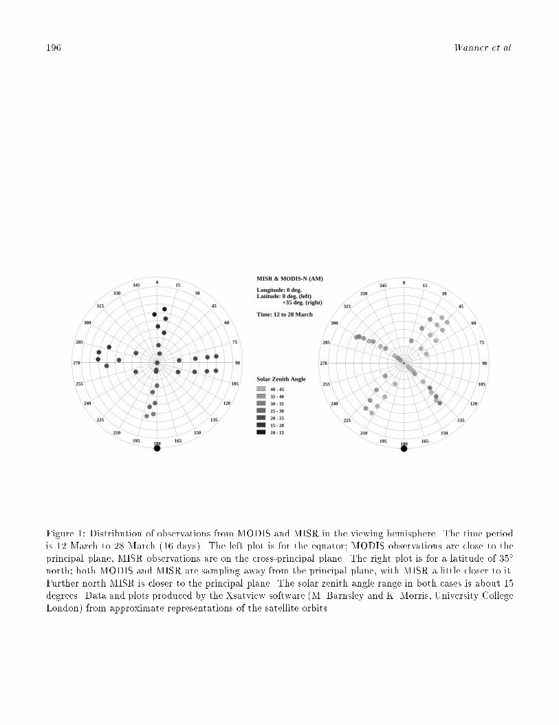
196 Wanner et al.
015
30
45
60
75
90
105
120
135
150
165180
195
210
225
240
255
270
285
300
315
330
345
10 - 15
15 - 20
20 - 25
25 - 30
30 - 35
35 - 40
40 - 45
Solar Zenith Angle
Time: 12 to 28 March
+35 deg. (right)Latitude: 0 deg. (left)Longitude: 0 deg.
MISR & MODIS-N (AM)0
15
30
45
60
75
90
105
120
135
150
165180
195
210
225
240
255
270
285
300
315
330
345
Figure 1: Distribution of observations from MODIS and MISR in the viewing hemisphere. The time periodis 12 March to 28 March (16 days). The left plot is for the equator; MODIS observations are close to theprincipal plane, MISR observations are on the cross-principal plane. The right plot is for a latitude of 35�
north; both MODIS and MISR are sampling away from the principal plane, with MISR a little closer to it.Further north MISR is closer to the principal plane. The solar zenith angle range in both cases is about 15degrees. Data and plots produced by the Xsatview software (M. Barnsley and K. Morris, University CollegeLondon) from approximate representations of the satellite orbits.
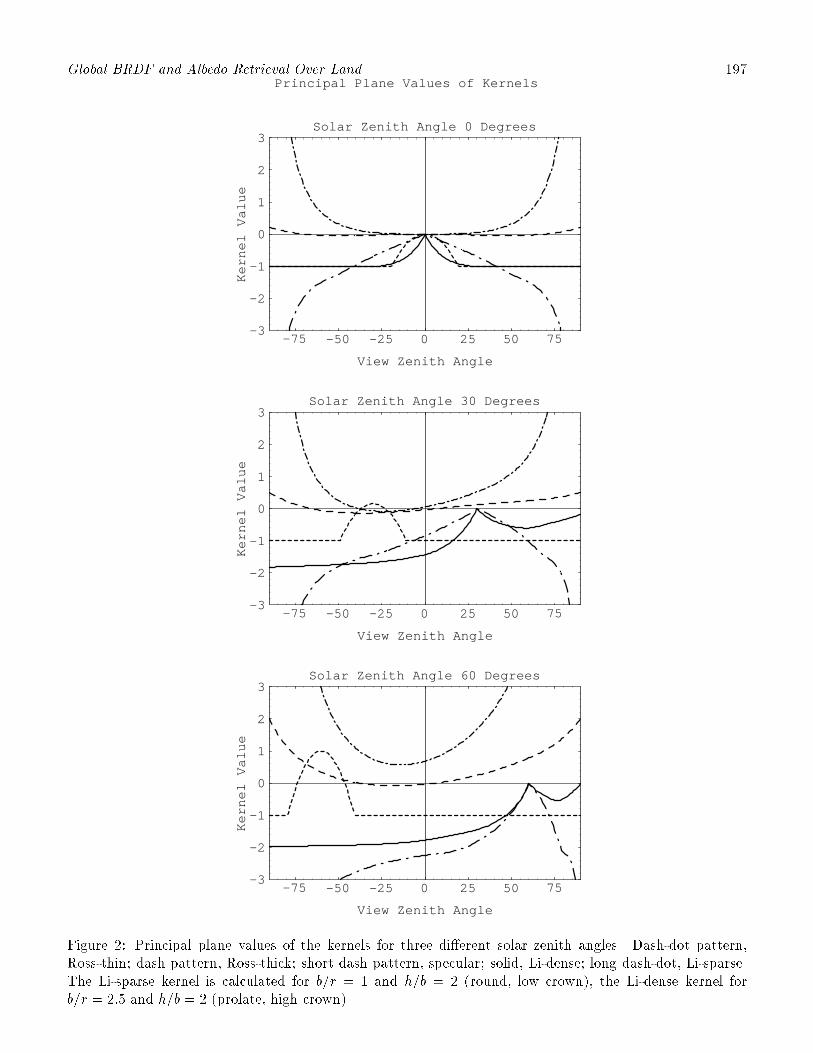
Global BRDF and Albedo Retrieval Over Land 197Principal Plane Values of Kernels
-75 -50 -25 0 25 50 75
View Zenith Angle
-3
-2
-1
0
1
2
3
Kernel Value
Solar Zenith Angle 60 Degrees
-75 -50 -25 0 25 50 75
View Zenith Angle
-3
-2
-1
0
1
2
3
Kernel Value
Solar Zenith Angle 30 Degrees
-75 -50 -25 0 25 50 75
View Zenith Angle
-3
-2
-1
0
1
2
3
Kernel Value
Solar Zenith Angle 0 Degrees
Figure 2: Principal plane values of the kernels for three di�erent solar zenith angles. Dash-dot pattern,Ross-thin; dash pattern, Ross-thick; short dash pattern, specular; solid, Li-dense; long dash-dot, Li-sparse.The Li-sparse kernel is calculated for b=r = 1 and h=b = 2 (round, low crown), the Li-dense kernel forb=r = 2:5 and h=b = 2 (prolate, high crown).
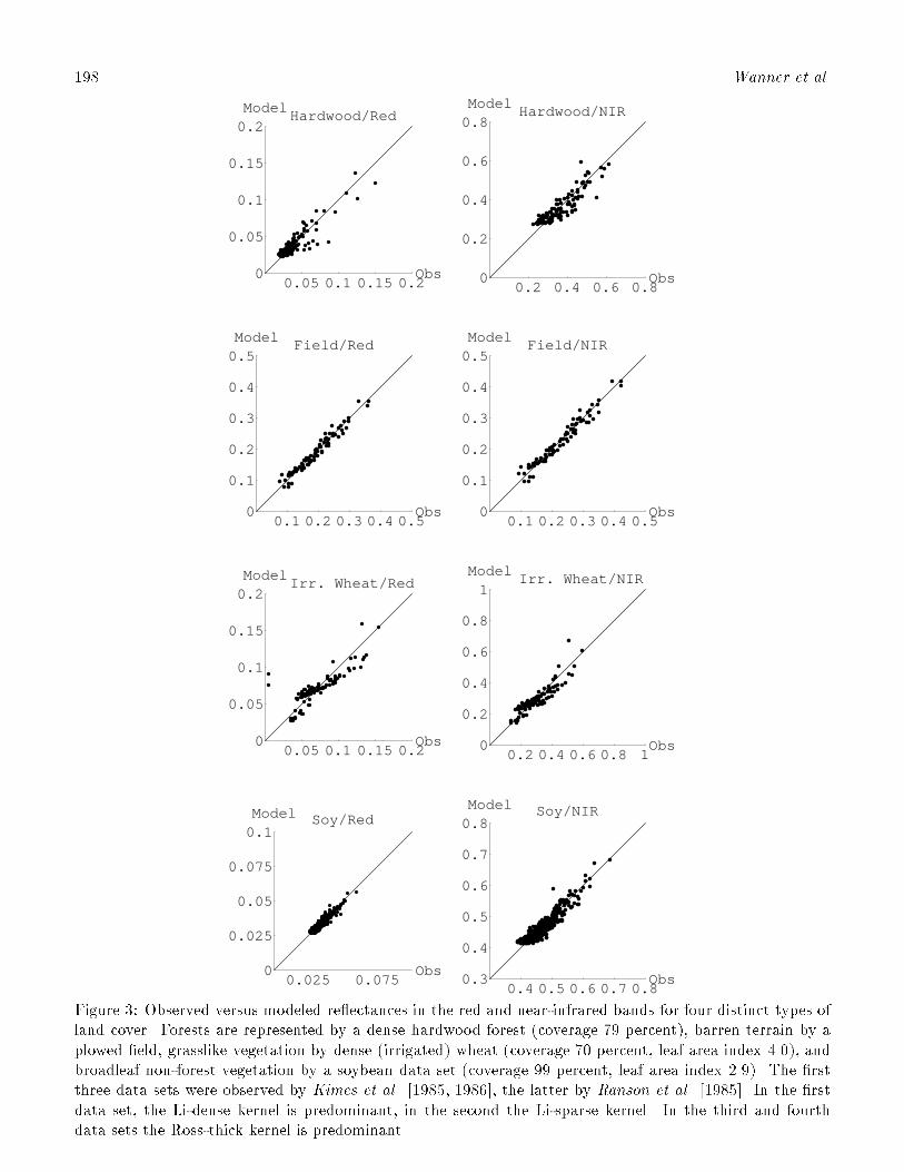
198 Wanner et al.
0.025 0.075Obs
Soy/Red
0
0.025
0.05
0.075
0.1Model
0.4 0.5 0.6 0.7 0.8Obs
Soy/NIR
0.3
0.4
0.5
0.6
0.7
0.8Model
0.05 0.1 0.15 0.2Obs
Irr. Wheat/Red
0
0.05
0.1
0.15
0.2Model
0.2 0.4 0.6 0.8 1Obs
Irr. Wheat/NIR
0
0.2
0.4
0.6
0.8
1Model
0.1 0.2 0.3 0.4 0.5Obs
Field/Red
0
0.1
0.2
0.3
0.4
0.5Model
0.1 0.2 0.3 0.4 0.5Obs
Field/NIR
0
0.1
0.2
0.3
0.4
0.5Model
0.05 0.1 0.15 0.2Obs
Hardwood/Red
0
0.05
0.1
0.15
0.2Model
0.2 0.4 0.6 0.8Obs
Hardwood/NIR
0
0.2
0.4
0.6
0.8Model
Figure 3: Observed versus modeled re ectances in the red and near-infrared bands for four distinct types ofland cover. Forests are represented by a dense hardwood forest (coverage 79 percent), barren terrain by aplowed �eld, grasslike vegetation by dense (irrigated) wheat (coverage 70 percent, leaf area index 4.0), andbroadleaf non-forest vegetation by a soybean data set (coverage 99 percent, leaf area index 2.9). The �rstthree data sets were observed by Kimes et al. [1985, 1986], the latter by Ranson et al. [1985]. In the �rstdata set, the Li-dense kernel is predominant, in the second the Li-sparse kernel. In the third and fourthdata sets the Ross-thick kernel is predominant.

Global BRDF and Albedo Retrieval Over Land 199
Root Band-Averaged Mean Absolute Deviation of Model (RMSE)
NS
ND
KS
KD
MW
model
Soy/Ranson
00.020.040.060.08
RMSE
NS
ND
KS
KD
MW
model
Soy/Kimes
00.020.040.060.08
RMSE
NS
ND
KS
KD
MW
model
Corn
00.020.040.060.08
RMSE
NS
ND
KS
KD
MW
model
Lawn
00.020.040.060.08
RMSE
NS
ND
KS
KD
MW
model
Irr. Wheat
00.020.040.060.08
RMSE
NS
ND
KS
KD
MW
model
Orch. Grass
00.020.040.060.08
RMSE
NS
ND
KS
KD
MW
model
Field
00.020.040.060.08
RMSE
NS
ND
KS
KD
MW
model
<5% Grass
00.020.040.060.08
RMSE
NS
ND
KS
KD
MW
model
Steppe
00.020.040.060.08
RMSE
NS
ND
KS
KD
MW
model
Hardwood
00.020.040.060.08
RMSE
NS
ND
KS
KD
MW
model
Pine
00.020.040.060.08
RMSE
NS
ND
KS
KD
MW
model
Aspen
00.020.040.060.08
RMSE
Figure 4: Root band averaged mean square errors (RMSE) of �tting �ve kernel-based BRDF model variantsto bidirectional re ectance data measured by Kimes [1983], Kimes et al. [1985, 1986], Deering et al. [1995]and Ranson et al. [1985] for 4 di�erent land cover types: top, forests; second row, barren or sparselyvegetated; third row, grasses and grasslike crops; bottom, broadleaf crops. Model codes are: N, Ross-thin;K, Ross-thick; S, Li-sparse; D, Li-dense; MW, modi�ed Walthall.

200 Wanner et al.
RMSE, White-Sky Albedo (Red and NIR), and Isotropic Reflectance Constant (Red and NIR)
NS
ND
KS
KD
MW
model
Soy
00.020.040.060.08
RMSE
NS
ND
KS
KD
MW
model
Soy
00.20.40.60.8WSA
NS
ND
KS
KD
MW
model
Soy
00.20.40.60.8R-ISO
NS
ND
KS
KD
MW
model
Hardwood
00.020.040.060.08
RMSE
NS
ND
KS
KD
MW
model
Hardwood
00.20.40.60.8WSA
NS
ND
KS
KD
MW
model
Hardwood
00.20.40.60.8R-ISO
Figure 5: Root band-averaged mean square errors (RMSE), white-sky albedo (WSA) and the isotropicmodel constant fi (nadir sun and view re ectances, R-ISO) of �ve kernel-based BRDF model variants tobidirectional re ectance data measured by Kimes et al. [1986], and Ranson et al. [1985] for two di�erentland cover types: forest and broadleaf crop. Model codes are: N, Ross-thin; K, Ross-thick; S, Li-sparse; D,Li-dense; MW, modi�ed Walthall.

ASAS Scaling Experiments 201
APPENDIX F:
ASAS SCALING EXPERIMENTS FOR BRDF MODEL INVERSION
(SUMMARY OF A PAPER BY MULLER AND DISNEY)

202 Muller and Disney
ASAS Scaling Experiments for BRDF Model Inversion
(Summary of a Paper by Muller and Disney)
It is extremely di�cult to extrapolate surface canopy directional re ectance measurements to pixel IFoVs of250m{1km which will be available with MODIS/MISR. Similarly it is important to establish what the linear-ity ranges of BRDF model inversions are if we are to set up a global validation network for MODIS/MISR-based BRDF or albedo.
There are two sources of airborne data which can be used to establish the scaling properties of the"Ambrals" models: ASAS (Irons et al., 1991) and POLDER (Roujean et al., 1996) .
Preliminary results are presented here for the use of ASAS data to investigate these scaling properties.A more comprehensive description of these experimental results will be described in (Muller and Disney,1997).
ASAS data has been geometrically registered to sub-pixel accuracy using the methods described in(Allison et al., 1994; Allison and Muller, 1992; Barnsley et al., 1995) . A schematic diagram of the methodis shown in Figure 1.
Two sites have been studied to date from the HAPEX-SAHEL experiment (Prince et al., 1995) : theSouthern Supersite millet area (hereafter referred to as SSS) and the West Central Supersite savannah/milletarea (hereafter referred to as WCSS).
The data were all atmospherically corrected using the "6S" scheme with the atmospheric optical depthmeasurements performed by Halthore (see (Brown de Coulstoun et al., 1996) ) by employing the US Standardatmosphere (1961) with a desert type aerosol. The aforementioned authors have suggested the use of atropical standard atmosphere with continental aerosol model which we have tested and which yields betterresults. The data is currently being re-processed using this new atmospheric correction data. An exampleof the "at surface" re ectance is shown for the SSS in Figure 2.
The resultant "at surface" re ectance data were spatially degraded using spatial averaging from theoriginal 3m resolution to 30m, 90m, 240m and 480m. The 9 look angles of ASAS only covered a 1.92 x 1.92km area so the results at 480m are only marginal. In future the POLDER data with 100m pixels over thesesame areas will be used to study the scaling up to 1km.
Each set of surface directional re ectances were then inverted using the "Ambrals" models to provide aper-pixel based model inversion. The BRDF models were solely chosen based on their minimum rmse. Theresults for all four TM-equivalent spectral bands (blue, green, red and NIR) are shown in Figures 3{5 forthe SSS and Figures 10{12 for the WCSS, where only resolutions 3m, 90m and 240m were selected here toserve as examples of the more extensive studies. For each model inversion an image was created of the rmsewhich are shown in Figures 7{9 for SSS and Figures 14{16 for the WCSS.
Histograms of the occurrence of each of the 9 models for each spectral band are shown in Figure 6 forthe SSS and Figure 13 for the WCSS.
The SSS model inversions and more clearly in the rmse results show artifacts associated with the numberof looks which were available outside of the central region which appear to have an impact on model selectionfrom 3m to 30m. The WCSS show no such artifacts. The SSS millet area indicates that as the resolutionis degraded the RossThickLiDense kernels are preferentially chosen over the modi�ed Walthall model. Asimilar behavior is also observed for the WCSS savannah/millet area with some slight evidence for a changeto RossThin at 480m.
The implications of this are that �eld canopy data or data taken from ASAS may produce di�erentmodel inversion results than that observed at MODIS/MISR wavelengths. This will be tested for all 6HAPEX-SAHEL sites in future and the results compared with those from the POLDER instrument.
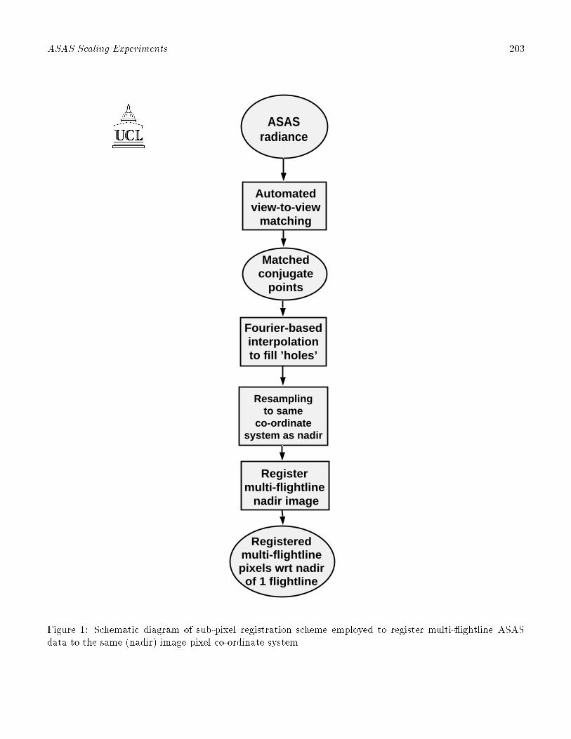
ASAS Scaling Experiments 203
ASASradiance
Automatedview-to-view
matching
Fourier-basedinterpolationto fill ’holes’
Registermulti-flightline nadir image
Registeredmulti-flightlinepixels wrt nadir
of 1 flightline
Matchedconjugate
points
Resamplingto same
co-ordinatesystem as nadir
Figure 1: Schematic diagram of sub-pixel registration scheme employed to register multi- ightline ASASdata to the same (nadir) image pixel co-ordinate system.
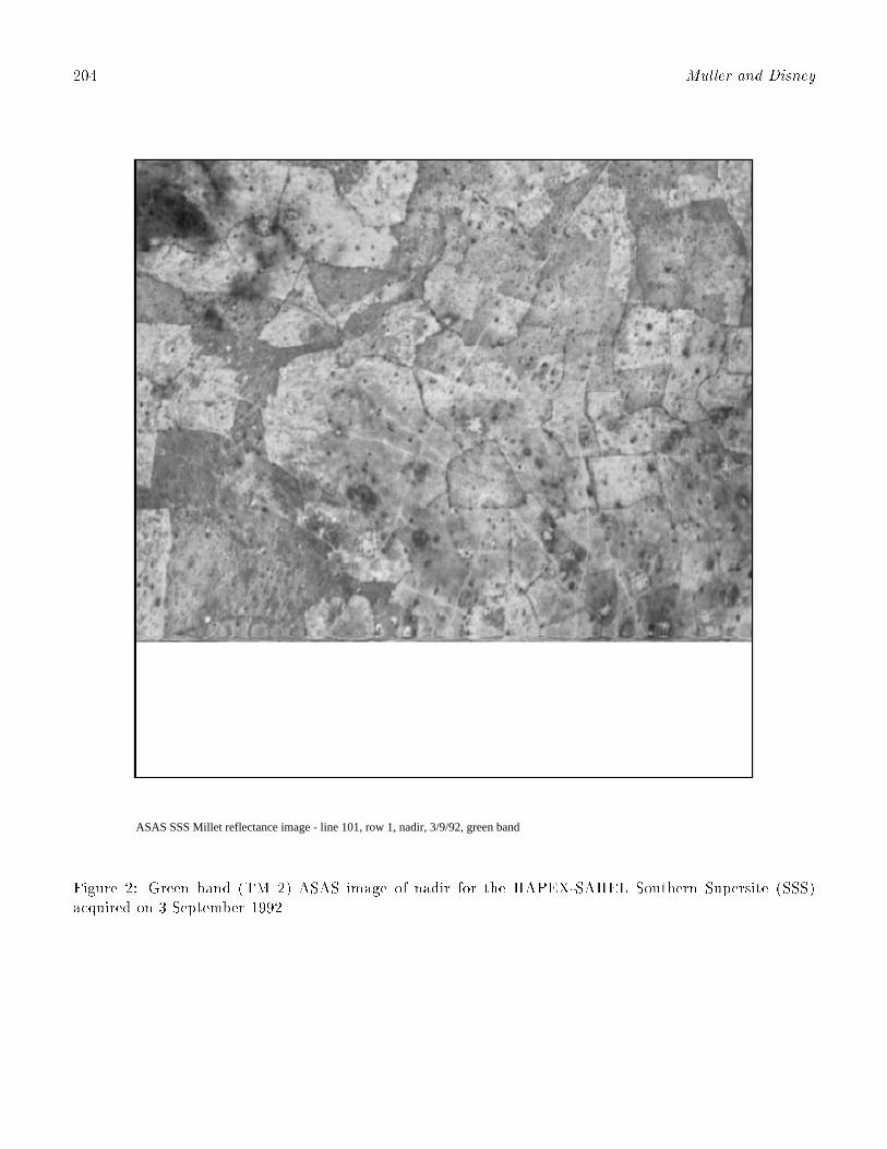
204 Muller and Disney
ASAS SSS Millet reflectance image - line 101, row 1, nadir, 3/9/92, green band
Figure 2: Green band (TM 2) ASAS image of nadir for the HAPEX-SAHEL Southern Supersite (SSS)acquired on 3 September 1992.
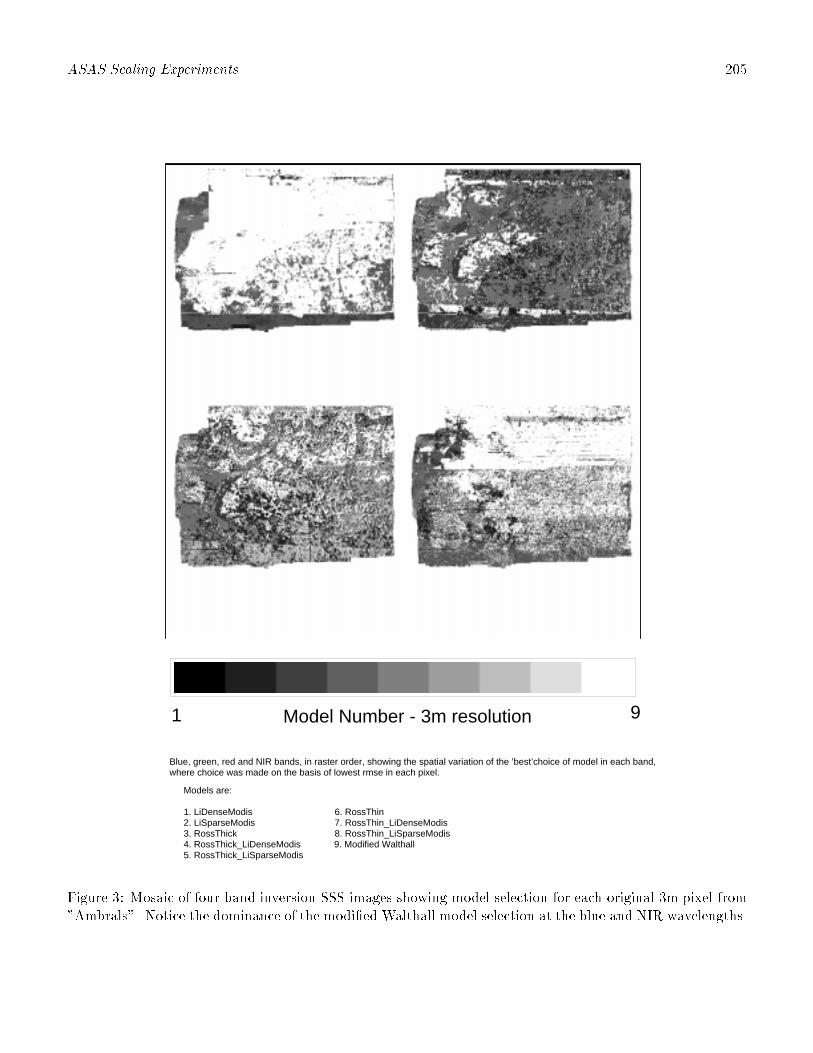
ASAS Scaling Experiments 205
Model Number - 3m resolution1 9
Blue, green, red and NIR bands, in raster order, showing the spatial variation of the ’best’choice of model in each band,where choice was made on the basis of lowest rmse in each pixel.
Models are:
1. LiDenseModis 6. RossThin2. LiSparseModis 7. RossThin_LiDenseModis3. RossThick 8. RossThin_LiSparseModis4. RossThick_LiDenseModis 9. Modified Walthall5. RossThick_LiSparseModis
Figure 3: Mosaic of four band inversion SSS images showing model selection for each original 3m pixel from"Ambrals". Notice the dominance of the modi�ed Walthall model selection at the blue and NIR wavelengths.
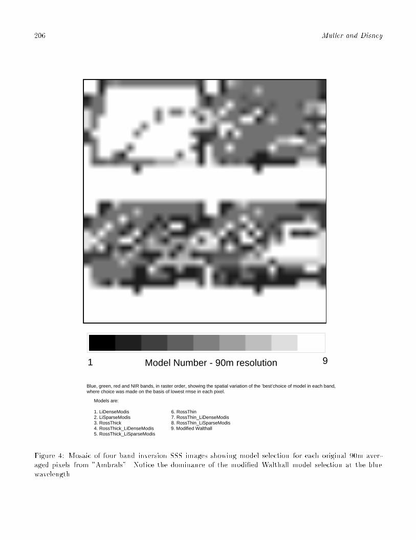
206 Muller and Disney
Model Number - 90m resolution1 9
Blue, green, red and NIR bands, in raster order, showing the spatial variation of the ’best’choice of model in each band,where choice was made on the basis of lowest rmse in each pixel.
Models are:
1. LiDenseModis 6. RossThin2. LiSparseModis 7. RossThin_LiDenseModis3. RossThick 8. RossThin_LiSparseModis4. RossThick_LiDenseModis 9. Modified Walthall5. RossThick_LiSparseModis
Figure 4: Mosaic of four band inversion SSS images showing model selection for each original 90m aver-aged pixels from "Ambrals". Notice the dominance of the modi�ed Walthall model selection at the bluewavelength.

ASAS Scaling Experiments 207
Model Number - 240m resolution1 9
Blue, green, red and NIR bands, in raster order, showing the spatial variation of the ’best’choice of model in each band,where choice was made on the basis of lowest rmse in each pixel.
Models are:
1. LiDenseModis 6. RossThin2. LiSparseModis 7. RossThin_LiDenseModis3. RossThick 8. RossThin_LiSparseModis4. RossThick_LiDenseModis 9. Modified Walthall5. RossThick_LiSparseModis
Figure 5: Mosaic of four band inversion SSS images showing model selection for each original 240m aver-aged pixels from "Ambrals". Notice the dominance of the modi�ed Walthall model selection at the bluewavelength.

208
Muller
andDisn
ey
0
2
4
6
8
10
12
0 2 4 6 8 10
Log (Frequency)
Model Number (see model images for key)
Frequency of occurrence for each BRDF model (green band - 565nm)
’3m_inversions/histo.2’’30m_inversions/histo.2’’90m_inversions/histo.2’
’240m_inversions/histo.2’’480m_inversions/histo.2’
0
2
4
6
8
10
12
0 2 4 6 8 10
Log (Frequency)
Model Number (see model images for key)
Frequency of occurrence for each BRDF model (blue band - 493nm)
’3m_inversions/histo.1’’30m_inversions/histo.1’’90m_inversions/histo.1’
’240m_inversions/histo.1’’480m_inversions/histo.1’
0
2
4
6
8
10
12
0 2 4 6 8 10
Log (Frequency)
Model Number (see model images for key)
Frequency of occurrence for each BRDF model (nir band - 839nm)
’3m_inversions/histo.4’’30m_inversions/histo.4’’90m_inversions/histo.4’
’240m_inversions/histo.4’’480m_inversions/histo.4’
0
2
4
6
8
10
12
0 2 4 6 8 10
Log (Frequency)
Model Number (see model images for key)
Frequency of occurrence for each BRDF model (red band - 662nm)
’3m_inversions/histo.3’’30m_inversions/histo.3’’90m_inversions/histo.3’
’240m_inversions/histo.3’’480m_inversions/histo.3’
Figure
6:Mosaic
offourbandinversio
nSSShistogram
sshow
ingfreq
uency
distrib
ution
ofmodelselection
.Notice
thedom
inance
oftheRossT
hick
LiDense
kern
elswhich
areselected
atresolu
tions>30m
andfor
lower
resolution
themodi�ed
Walth
allare
preferen
tiallyselected
.
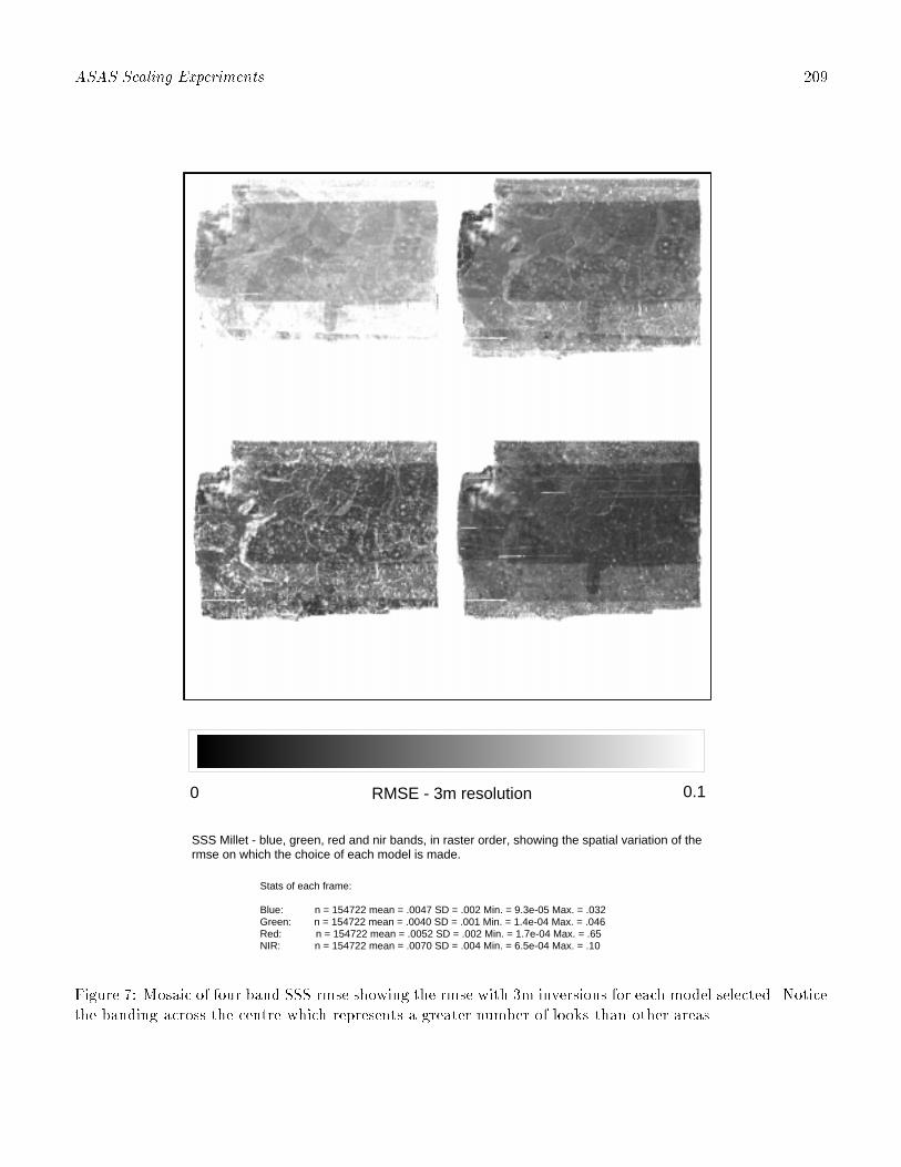
ASAS Scaling Experiments 209
RMSE - 3m resolution0 0.1
SSS Millet - blue, green, red and nir bands, in raster order, showing the spatial variation of thermse on which the choice of each model is made.
Stats of each frame:
Blue: n = 154722 mean = .0047 SD = .002 Min. = 9.3e-05 Max. = .032Green: n = 154722 mean = .0040 SD = .001 Min. = 1.4e-04 Max. = .046Red: n = 154722 mean = .0052 SD = .002 Min. = 1.7e-04 Max. = .65NIR: n = 154722 mean = .0070 SD = .004 Min. = 6.5e-04 Max. = .10
Figure 7: Mosaic of four band SSS rmse showing the rmse with 3m inversions for each model selected. Noticethe banding across the centre which represents a greater number of looks than other areas.

210 Muller and Disney
RMSE - 90m resolution0 .051
SSS Millet - blue, green, red and nir bands, in raster order, showing the spatial variation of thermse on which the choice of each model is made.
Stats of each frame:
Blue: n = 198 mean = .0036 SD = .001 Min. = 1.4e-04 Max. = .0097Green: n = 198 mean = .0050 SD = .003 Min. = 3.8e-04 Max. = .0178Red: n = 198 mean = .0073 SD = .005 Min. = 7.0e-04 Max. = .030NIR: n = 198 mean = .0130 SD = .009 Min. = 13e-04 Max. = .051
Figure 8: Mosaic of four band SSS rmse showing the rmse with 90m inversions for each model selected.Notice the banding is reduced with respect to 3m and 30m inversions across the centre which represents agreater number of looks than other areas.

ASAS Scaling Experiments 211
RMSE - 240m resolution0 .03
SSS Millet - blue, green, red and nir bands, in raster order, showing the spatial variation of thermse on which the choice of each model is made.
Stats of each frame:
Blue: n = 36 mean = .0039 SD = .0007 Min. = 2.1e-03 Max. = .0052Green: n = 36 mean = .0066 SD = .0016 Min. = 3.3e-03 Max. = .0096Red: n = 36 mean = .0104 SD = .0032 Min. = 6.0e-03 Max. = .0170NIR: n = 36 mean = .0190 SD = .0060 Min. = 8.0e-03 Max. = .0291
Figure 9: Mosaic of four band SSS rmse showing the rmse with 90m inversions for each model selected.Notice the banding has now disappeared.
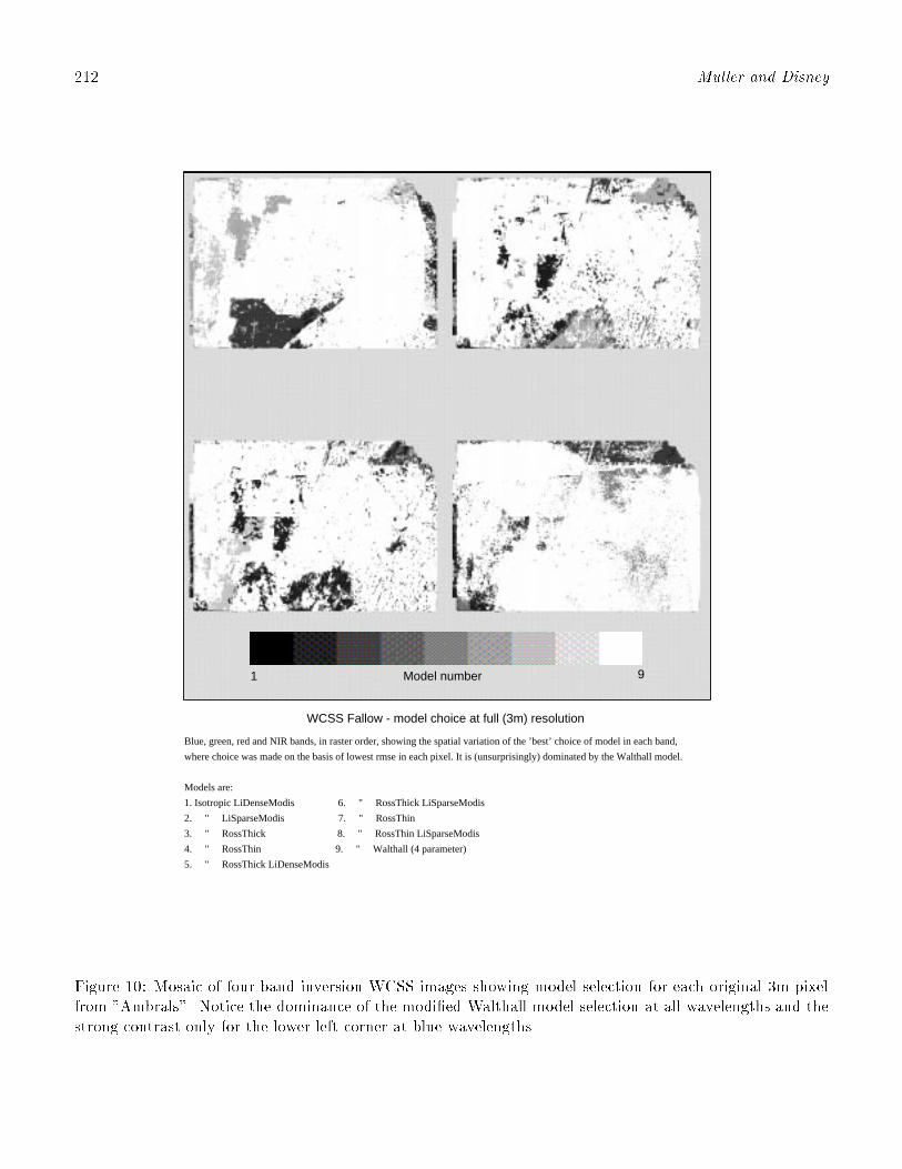
212 Muller and Disney
Blue, green, red and NIR bands, in raster order, showing the spatial variation of the ’best’ choice of model in each band,
where choice was made on the basis of lowest rmse in each pixel. It is (unsurprisingly) dominated by the Walthall model.
Models are:
1. Isotropic LiDenseModis 6. " RossThick LiSparseModis
2. " LiSparseModis 7. " RossThin
3. " RossThick 8. " RossThin LiSparseModis
4. " RossThin 9. " Walthall (4 parameter)
5. " RossThick LiDenseModis
1 9Model number
WCSS Fallow - model choice at full (3m) resolution
Figure 10: Mosaic of four band inversion WCSS images showing model selection for each original 3m pixelfrom "Ambrals". Notice the dominance of the modi�ed Walthall model selection at all wavelengths and thestrong contrast only for the lower left corner at blue wavelengths.

ASAS Scaling Experiments 213
Blue, green, red and NIR bands, in raster order, showing the spatial variation of the ’best’ choice of model in each band,
where choice was made on the basis of lowest rmse in each pixel. It is (unsurprisingly) dominated by the Walthall model.
Models are:
1. Isotropic LiDenseModis 6. " RossThick LiSparseModis
2. " LiSparseModis 7. " RossThin
3. " RossThick 8. " RossThin LiSparseModis
4. " RossThin 9. " Walthall (4 parameter)
5. " RossThick LiDenseModis
1 9Model Number
WCSS Fallow - model choice at 90m resolution
Figure 11: Mosaic of four band inversion WCSS images showing model selection for each original 90m pixelfrom "Ambrals". Notice the dominance of the RossThickLiDense model selection at all wavelengths.
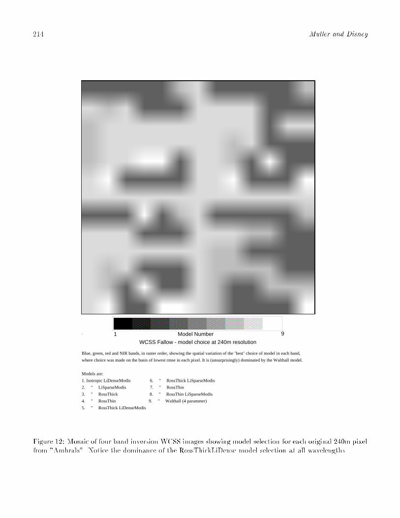
214 Muller and Disney
.
Blue, green, red and NIR bands, in raster order, showing the spatial variation of the ’best’ choice of model in each band,
where choice was made on the basis of lowest rmse in each pixel. It is (unsurprisingly) dominated by the Walthall model.
Models are:
1. Isotropic LiDenseModis 6. " RossThick LiSparseModis
2. " LiSparseModis 7. " RossThin
3. " RossThick 8. " RossThin LiSparseModis
4. " RossThin 9. " Walthall (4 parameter)
5. " RossThick LiDenseModis
1 9Model Number
WCSS Fallow - model choice at 240m resolution
Figure 12: Mosaic of four band inversion WCSS images showing model selection for each original 240m pixelfrom "Ambrals". Notice the dominance of the RossThickLiDense model selection at all wavelengths.

ASASScalin
gExperim
ents
215
0
2
4
6
8
10
12
0 2 4 6 8 10
Log frequency
Model Number
Log frequncy of occurrence for each BRDF model (green band - 565nm)
’3m_inversions.histo.2’’30m_inversions.histo.2’’90m_inversions.histo.2’
’240m_inversions.histo.2’’480m_inversions.histo.2’
0
2
4
6
8
10
12
0 2 4 6 8 10
Log frequency
Model Number
Log frequncy of occurrence for each BRDF model (blue band - 493nm)
’3m_inversions.histo.1’’30m_inversions.histo.1’’90m_inversions.histo.1’
’240m_inversions.histo.1’’480m_inversions.histo.1’
0
2
4
6
8
10
12
0 2 4 6 8 10
Log frequency
Model Number
Log frequncy of occurrence for each BRDF model (NIR band - 839nm)
’3m_inversions.histo.4’’30m_inversions.histo.4’’90m_inversions.histo.4’
’240m_inversions.histo.4’’480m_inversions.histo.4’
0
2
4
6
8
10
12
0 2 4 6 8 10
Log frequency
Model Number
Log frequncy of occurrence for each BRDF model (red band - 662nm)
’3m_inversions.histo.3’’30m_inversions.histo.3’’90m_inversions.histo.3’
’240m_inversions.histo.3’’480m_inversions.histo.3’
Figure13:
Mosaic
offourbandinversion
WCSShistogram
sshow
ingfreq
uency
distrib
ution
ofmodelselection
.Notice
thedom
inance
oftheWalth
allmodelkern
elsupto
30mandthen
theRossT
hick
LiDense
kernels
up
to240m
andtheRossT
hin
modelat480m
.
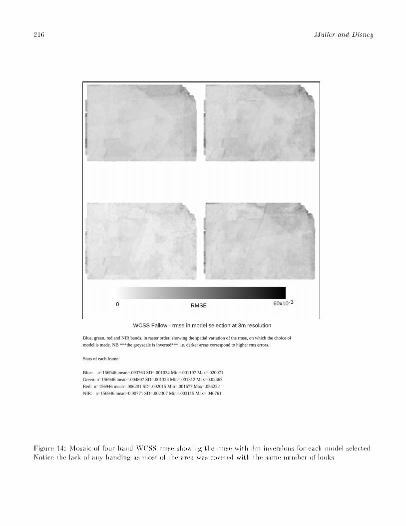
216 Muller and Disney
Blue, green, red and NIR bands, in raster order, showing the spatial variation of the rmse, on which the choice of
model is made. NB ***the greyscale is inverted*** i.e. darker areas correspond to higher rms errors.
Stats of each frame:
Blue: n=156946 mean=.003763 SD=.001034 Min=.001197 Max=.020071
Green: n=156946 mean=.004807 SD=.001323 Min=.001312 Max=0.02363
Red: n=156946 mean=.006201 SD=.002015 Min=.001677 Max=.054222
NIR: n=156946 mean=0.00771 SD=.002307 Min=.003115 Max=.040761
0 60x10-3RMSE
WCSS Fallow - rmse in model selection at 3m resolution
Figure 14: Mosaic of four band WCSS rmse showing the rmse with 3m inversions for each model selected.Notice the lack of any banding as most of the area was covered with the same number of looks.
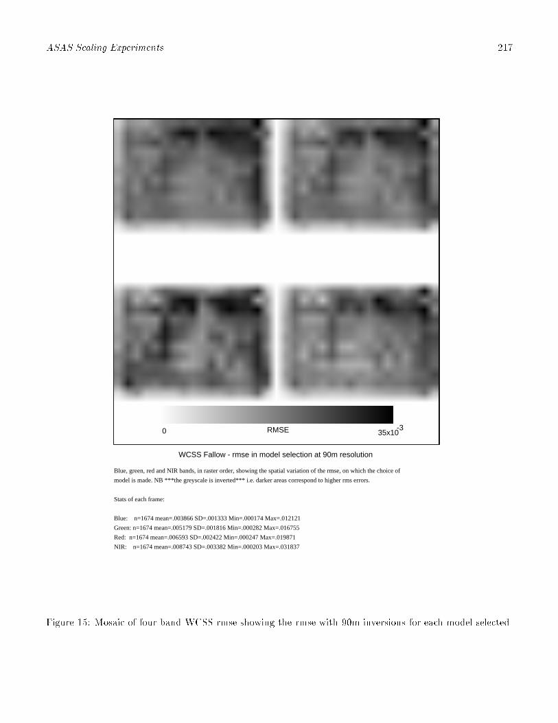
ASAS Scaling Experiments 217
Blue, green, red and NIR bands, in raster order, showing the spatial variation of the rmse, on which the choice of
model is made. NB ***the greyscale is inverted*** i.e. darker areas correspond to higher rms errors.
Stats of each frame:
Blue: n=1674 mean=.003866 SD=.001333 Min=.000174 Max=.012121
Green: n=1674 mean=.005179 SD=.001816 Min=.000282 Max=.016755
Red: n=1674 mean=.006593 SD=.002422 Min=.000247 Max=.019871
NIR: n=1674 mean=.008743 SD=.003382 Min=.000203 Max=.031837
0 35x10-3RMSE
WCSS Fallow - rmse in model selection at 90m resolution
Figure 15: Mosaic of four band WCSS rmse showing the rmse with 90m inversions for each model selected.

218 Muller and Disney
.
Blue, green, red and NIR bands, in raster order, showing the spatial variation of the rmse, on which the choice of
model is made. NB ***the greyscale is inverted*** i.e. darker areas correspond to higher rms errors.
Stats of each frame:
Blue: n=36 mean=.004195 SD=.001338 Min=.002073 Max=.006569
Green: n=36 mean=.006229 SD=.001743 Min=.003191 Max=.009263
Red: n=36 mean=.009075 SD=.002667 Min=.004554 Max=0.01508
NIR: n=36 mean=.011941 SD=.002479 Min=.008005 Max=.016868
0 20x10-3
RMSE
WCSS Fallow - rmse in model selection at 240m resolution
Figure 16: Mosaic of four band WCSS rmse showing the rmse with 240m inversions for each model selected.

Landsat-TM Spectral Albedo Extraction 219
APPENDIX G:
LANDSAT-TM SPECTRAL ALBEDO EXTRACTION (SUMMARY
OF A PAPER BY DISNEY, MULLER ET AL.)
220 Disney, Muller et al.
Landsat-TM Spectral Albedo Extraction
(Summary of a Paper by Disney, Muller et al.)
An attempt has been made to use the ASAS "at surface" re ectances to create a large area BRDF/albedomap for use in scaling studies and simulation studies for GCM and hydrological applications. See (Disneyet al., 1997; Muller et al., 1997b) for a fuller discussion.
The overall processing scheme is shown in Figure 1 which includes details of the atmospheric correctionscheme for the ASAS data. (see Appendix XXX for a fuller discussion of this issue).
The resultant ASAS "at surface" radiances for each of the 4 TM spectral bands (1{4) were spatiallydegraded to TM 30m resolution and registered to the geocoded surface re ectance TM pixels provided bythe NASA EDC DAAC to support MODIS Land group validation e�orts. The radiometric range of the pixelsfrom ASAS were then adjusted to �t the TM values. All of these pixels were then used as training statisticsfor the 3 regions covered in the SSS (millet, savannah/fallow and tiger bush). A Maximum Likelihoodclassi�cation was then performed of the TM pixels using these training statistics and for each classi�edpixel, the original albedo value associated with that pixel was used to predict a spectral albedo for all theclassi�ed TM pixels.
The resultant TM spectral albedo maps are shown in Figure 2 (using the modi�ed Walthall model) andfor the RossThick-LiSparse model in Figure 3. Notice the AGRYMET agricultural square which is clearlyin both images as well as the tiger bush in the lower left corner. The spectral albedo values are di�erentdependent on the model with the RossThick-LiSparse model values being higher.
In future the "Ambrals" model inversions will be used from the 30m scaling experiments to repeat theexperiment. Narrowband to broadband conversion will be made using the method proposed by (Brest andGoward, 1987) and the resultant broadband albedos will be compared to �eld solarimeter-based albedosprovided by Simon Allen and his colleagues (Allen et al., 1994) at the Institute of Hydrology, Wallingfordfor validation. A similar procedure will also be tested using the POLDER data.

Landsat-TM Spectral Albedo Extraction 221
ASASco-registered
radiance
6satmosphericcorrection
BRDF model inversion algorithms
BRDF modelsranked byr.m.s. error
Hemisphericalintegration
Spectral"albedo maps"
’at ground’reflectances
Optical depthinformation
Degrade nadir ASAS images to TM res.;
select same area in TM; match
radiometric info.
Derive training stats from transformed ASAS data; use to ’classify’ TM data
Results mapped through from small areas to
TM scenes
Figure 1: Schematic ow diagram of the LANDSAT-TM spectral albedo derivation using the ASAS direc-tional re ectances including the production of "at surface" re ectances using the atmospheric optical depthmeasurements from Halthore.

222 Disney, Muller et al.
Bands 1,2,3 and 4 (left to right, top to bottom) of albedo, mapped from ASAS model inversions up to
TM-scale. The BRDF kernels used in this case were the Isotropic, WalthallLinMultCos, WalthallSqMult
and WalthallSqSum (i.e. Modified walthall model).
A 3 x 3 convolution filter was passed over the images to remove high frequency noise in the images.
The stats of the raw images are as follows:
Band 1 - n=129414 mean=.048008 SD=.018297 Min=7.96096e-05 Max=.082251
Band 2 - n=129414 mean=.120139 SD=0.03855 Min=.000873 Max=.177322
Band 3 - n=129414 mean=.181225 SD=.061481 Min=.000972 Max=.290579
Band 4 - n=129414 mean=.348764 SD=.094025 Min=.005047 Max=.439253
Albedo maps of SSS at TM resolution
Figure 2: Mosaic of LANDSAT-TM spectral albedos for the four spectral bands using a modi�ed Walthallinversion model for the ASAS \at surface" directional re ectances.

Landsat-TM Spectral Albedo Extraction 223
Bands 1,2,3 and 4 (left to right, top to bottom) of albedo, mapped from ASAS model inversions up
to TM-scale. The BRDF kernels used in this case were the Isotropic, RossThick and LiSparseModis.
A 3 x 3 convolution filter was passed over the images to remove high frequency noise in the images.
The stats of the raw images are as follows:
Band 1 - n=175011 mean=.049615 SD=.018106 Min=.000334 Max=.082018
Band 2 - n=175011 mean=.118947 SD=.035053 Min=.000972 Max=.177611
Band 3 - n=175011 mean=.180364 SD=.057442 Min=.001486 Max=.295627
Band 4 - n=175011 mean=.351156 SD=.072161 Min=.004554 Max=.446293
Figure 3: Mosaic of LANDSAT-TM spectral albedos for the four spectral bands using a RossThickLiSparsemodel inversion for the ASAS "at surface" directional re ectances. Notice the higher values of spectralalbedo values calculated cf. modi�ed Walthall in previous �gure.

224 Muller, Disney and Lewis
APPENDIX H:
MONTE CARLO-RAY TRACING SIMULATIONS OF ASAS (SUM-
MARY OF A PAPER BY MULLER, DISNEY AND LEWIS)
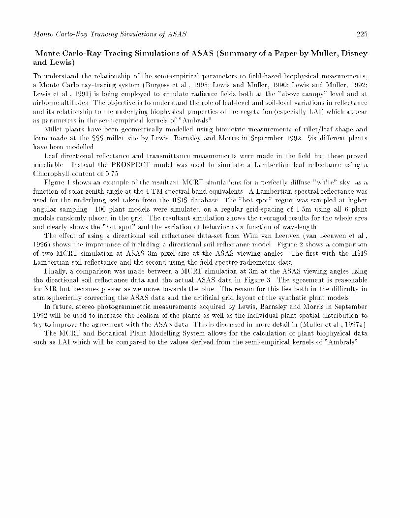
Monte Carlo-Ray Trancing Simulations of ASAS 225
Monte Carlo-Ray Tracing Simulations of ASAS (Summary of a Paper by Muller, Disney
and Lewis)
To understand the relationship of the semi-empirical parameters to �eld-based biophysical measurements,a Monte Carlo ray-tracing system (Burgess et al., 1995; Lewis and Muller, 1990; Lewis and Muller, 1992;Lewis et al., 1991) is being employed to simulate radiance �elds both at the "above canopy" level and atairborne altitudes. The objective is to understand the role of leaf-level and soil-level variations in re ectanceand its relationship to the underlying biophysical properties of the vegetation (especially LAI) which appearas parameters in the semi-empirical kernels of "Ambrals".
Millet plants have been geometrically modelled using biometric measurements of tiller/leaf shape andform made at the SSS millet site by Lewis, Barnsley and Morris in September 1992. Six di�erent plantshave been modelled.
Leaf directional re ectance and transmittance measurements were made in the �eld but these provedunreliable. Instead the PROSPECT model was used to simulate a Lambertian leaf re ectance using aChlorophyll content of 0.75.
Figure 1 shows an example of the resultant MCRT simulations for a perfectly di�use "white" sky. as afunction of solar zenith angle at the 4 TM spectral band equivalents. A Lambertian spectral re ectance wasused for the underlying soil taken from the HSIS database. The "hot spot" region was sampled at higherangular sampling. 100 plant models were simulated on a regular grid-spacing of 1.5m using all 6 plantmodels randomly placed in the grid. The resultant simulation shows the averaged results for the whole areaand clearly shows the "hot spot" and the variation of behavior as a function of wavelength.
The e�ect of using a directional soil re ectance data-set from Wim van Leeuven (van Leeuwen et al.,1996) shows the importance of including a directional soil re ectance model. Figure 2 shows a comparisonof two MCRT simulation at ASAS 3m pixel size at the ASAS viewing angles. The �rst with the HSISLambertian soil re ectance and the second using the �eld spectro-radiometric data.
Finally, a comparison was made between a MCRT simulation at 3m at the ASAS viewing angles usingthe directional soil re ectance data and the actual ASAS data in Figure 3. The agreement is reasonablefor NIR but becomes poorer as we move towards the blue. The reason for this lies both in the di�culty inatmospherically correcting the ASAS data and the arti�cial grid layout of the synthetic plant models.
In future, stereo photogrammetric measurements acquired by Lewis, Barnsley and Morris in September1992 will be used to increase the realism of the plants as well as the individual plant spatial distribution totry to improve the agreement with the ASAS data. This is discussed in more detail in (Muller et al., 1997a).
The MCRT and Botanical Plant Modelling System allows for the calculation of plant biophysical datasuch as LAI which will be compared to the values derived from the semi-empirical kernels of "Ambrals"

226
Muller,
Disn
eyandLew
is
0.1
0.12
0.14
0.16
0.18
0.2
0.22
0.24
-80 -60 -40 -20 0 20 40 60 80
Reflectance
View Zenith Angle/deg
Simulated Reflectance Against VZA, varying SZA (570.2nm)
’refl.0.band_2’’refl.10.band_2’’refl.20.band_2’’refl.30.band_2’’refl.40.band_2’’refl.50.band_2’’refl.60.band_2’’refl.70.band_2’
0.05
0.06
0.07
0.08
0.09
0.1
0.11
0.12
0.13
0.14
0.15
-80 -60 -40 -20 0 20 40 60 80
Reflectance
View Zenith Angle/deg
Simulated Reflectance Against VZA, varying SZA (498.5nm)
’refl.0.band_1’’refl.10.band_1’’refl.20.band_1’’refl.30.band_1’’refl.40.band_1’’refl.50.band_1’’refl.60.band_1’’refl.70.band_1’
0.3
0.35
0.4
0.45
0.5
0.55
0.6
-80 -60 -40 -20 0 20 40 60 80
Reflectance
View Zenith Angle/deg
Simulated Reflectance Against VZA, varying SZA (843.5nm)
’refl.0.band_4’’refl.10.band_4’’refl.20.band_4’’refl.30.band_4’’refl.40.band_4’’refl.50.band_4’’refl.60.band_4’’refl.70.band_4’
0.16
0.18
0.2
0.22
0.24
0.26
0.28
0.3
0.32
0.34
-80 -60 -40 -20 0 20 40 60 80
Reflectance
View Zenith Angle/deg
Simulated Reflectance Against VZA, varying SZA (666.9nm)
’refl.0.band_3’’refl.10.band_3’’refl.20.band_3’’refl.30.band_3’’refl.40.band_3’’refl.50.band_3’’refl.60.band_3’’refl.70.band_3’
Figure
1:Monte
Carlo
ray-traced
simulation
sof
direction
alre
ectance
plots
asafunction
ofsolar
zenith
angleusin
gall
6plantmodels
randomly
placed
ona10
x10
grid.Thevalu
esshow
nhere
arethemean
valuefor
thewhole
area.
Awhite
(single
di�use)
skyhas
been
used
.View
andsolar
zenith
angle
sampling
isat
10degrees
excep
tarou
ndthe�
10degrees
ofthe"hot
spot"
where
thesam
plingisat
2degrees.
The
plan
tsare
modelled
geometrically
from
biometric
�eld
measu
rements.
Theleaf
re ectan
ce/transm
ittance
isassu
med
isotropicandisderived
from
thePROSPECTmodel.
Thesoil
re ectan
cemeasu
rementsare
takenfrom
theHSIS
data-b
ase.

Monte
Carlo
-RayTrancin
gSim
ulatio
nsofASAS
227
0
0.05
0.1
0.15
0.2
0.25
0.3
0.35
0.4
0.45
-60 -40 -20 0 20 40 60 80
Reflectance
View Zenith Angle/deg
Simulated ASAS Refl. with & w/out soil direct. refl.(SZA=34 deg.; dry soil,xpp)
’refl.dry.op.band.1’’refl.dry.op.band.2’’refl.dry.op.band.3’’refl.dry.op.band.4’
’refl.34.band_1’’refl.34.band_2’’refl.34.band_3’’refl.34.band_4’
0
0.05
0.1
0.15
0.2
0.25
0.3
0.35
0.4
0.45
-60 -40 -20 0 20 40 60 80
Reflectance
View Zenith Angle/deg
Simulated ASAS Refl. with & w/out soil direct. refl.(SZA=34 deg.; dry soil,pp)
’refl.dry.pp.band.1’’refl.dry.pp.band.2’’refl.dry.pp.band.3’’refl.dry.pp.band.4’
’refl.34.band_1’’refl.34.band_2’’refl.34.band_3’’refl.34.band_4’
0
0.05
0.1
0.15
0.2
0.25
0.3
0.35
0.4
0.45
-60 -40 -20 0 20 40 60 80
Reflectance
View Zenith Angle/deg
Simulated ASAS Refl. with & w/out soil direct. refl.(SZA=34 deg.; wet soil,xpp)
’refl.wet.op.band.1’’refl.wet.op.band.2’’refl.wet.op.band.3’’refl.wet.op.band.4’
’refl.34.band_1’’refl.34.band_2’’refl.34.band_3’’refl.34.band_4’
0
0.05
0.1
0.15
0.2
0.25
0.3
0.35
0.4
0.45
-60 -40 -20 0 20 40 60 80
Reflectance
View Zenith Angle/deg
Simulated ASAS Refl. with & w/out soil direct. refl.(SZA=34 deg.; wet soil,pp)
’refl.wet.pp.band.1’’refl.wet.pp.band.2’’refl.wet.pp.band.3’’refl.wet.pp.band.4’
’refl.34.band_1’’refl.34.band_2’’refl.34.band_3’’refl.34.band_4’
Figure
2:Monte
Carlo
ray-traced
simulation
sat
theASASview
angles
ofdirection
alre
ectance
plots
asafunctio
nofsola
rzen
ithangle
usin
gall6plan
tmodels
random
lyplaced
ona10
x10
grid.Thevalu
esshow
nhere
arethemeanvaluefora3m
area.
Awhite
(single
di�use)
skyhas
been
used
.Solar
zenith
angle
samplingisat34degrees.
Theplan
tsare
modelled
geometrically
frombiom
etric�eld
measu
rements.
The
leafre
ectance/
transm
ittance
isassu
med
isotropicandisderived
fromthePROSPECT
model.
Thesoil
re ecta
nce
measu
rements
aretaken
from
theHSIS
datab
aseandare
compared
with
theSpectron
SE-590
spectro
-radiom
etricdata
taken
byWim
vanLeeu
venfrom
theWCSS.

228
Muller,
Disn
eyandLew
is
0
0.05
0.1
0.15
0.2
0.25
0.3
0.35
0.4
0.45
0.5
-60 -40 -20 0 20 40 60 80
Ref
lect
ance
View Zenith Angle (deg.)
ASAS SSS Millet reflectance compared to MCRT Simulated Millet Reflectances
’ASAS_blue.refl’’ASAS_green.refl’
’ASAS_red.refl’’ASAS_nir.refl’
’MCRT_blue.refl’’MCRT_green.refl’
’MCRT_red.refl’’MCRT_nir.refl’
Figure
3:Com
parison
ofASAS"at
surface"
re ectan
cefrom
theSSSwith
MCRTsim
ulation
sof
thesam
earea
.TheMCRTsim
ulation
suses
all6plan
tmodels
random
lyplaced
ona10
x10
grid.Thevalu
esshow
nhere
are
themeanvaluefor
a3m
area.Awhite
(single
di�use)
skyhas
been
used
.Theplan
tsare
modelled
geometrica
llyfrom
biometric
�eld
measu
rements.
Theleaf
re ectan
ce/transm
ittance
isassu
med
isotropic
andisderiv
edfrom
thePROSPECTmodel.
Thesoil
re ectan
cemeasu
rementsare
taken
fromtheSpectron
SE-590spectro-rad
iometric
data
taken
byWim
vanLeeu
ven
fromtheWCSS.

AVHRR Inversions Using Kernel-Driven BRDF Models 229
APPENDIX I:
MONITORING LAND SURFACEDYNAMICS IN THEHAPEX-SAHEL
AREA USING KERNEL-DRIVEN BRDF MODELS AND AVHRR
DATA (SUMMARY OF A PAPER BY RUIZ DE LOPE AND LEWIS)
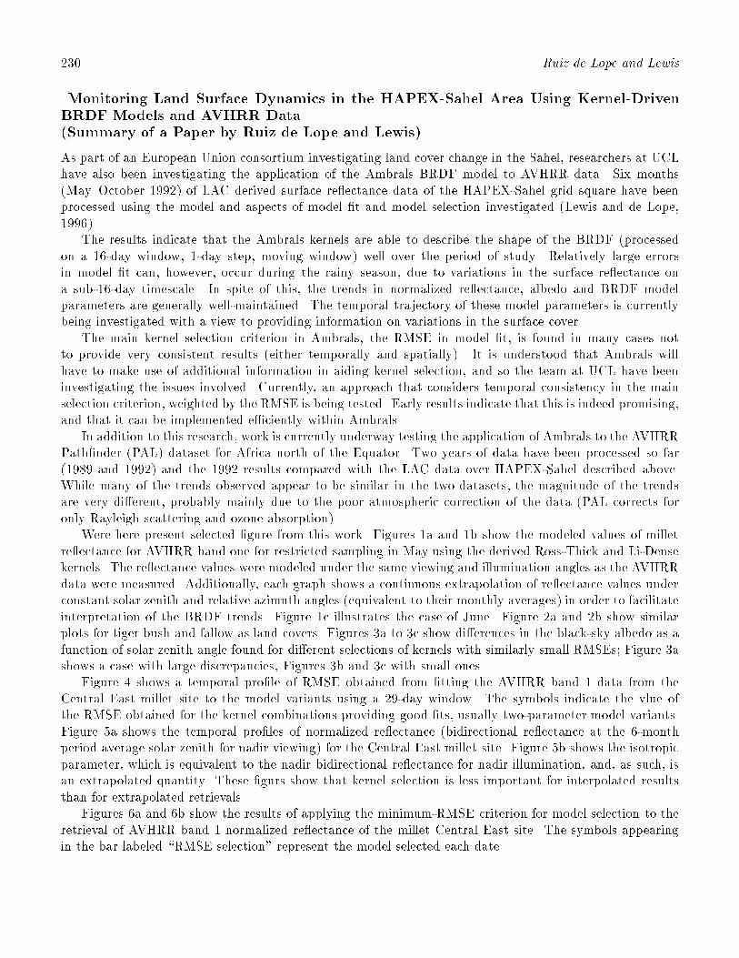
230 Ruiz de Lope and Lewis
Monitoring Land Surface Dynamics in the HAPEX-Sahel Area Using Kernel-Driven
BRDF Models and AVHRR Data
(Summary of a Paper by Ruiz de Lope and Lewis)
As part of an European Union consortium investigating land cover change in the Sahel, researchers at UCLhave also been investigating the application of the Ambrals BRDF model to AVHRR data. Six months(May{October 1992) of LAC derived surface re ectance data of the HAPEX-Sahel grid square have beenprocessed using the model and aspects of model �t and model selection investigated (Lewis and de Lope,1996).
The results indicate that the Ambrals kernels are able to describe the shape of the BRDF (processedon a 16-day window, 1-day step, moving window) well over the period of study. Relatively large errorsin model �t can, however, occur during the rainy season, due to variations in the surface re ectance ona sub-16-day timescale. In spite of this, the trends in normalized re ectance, albedo and BRDF modelparameters are generally well-maintained. The temporal trajectory of these model parameters is currentlybeing investigated with a view to providing information on variations in the surface cover.
The main kernel selection criterion in Ambrals, the RMSE in model �t, is found in many cases notto provide very consistent results (either temporally and spatially). It is understood that Ambrals willhave to make use of additional information in aiding kernel selection, and so the team at UCL have beeninvestigating the issues involved. Currently, an approach that considers temporal consistency in the mainselection criterion, weighted by the RMSE is being tested. Early results indicate that this is indeed promising,and that it can be implemented e�ciently within Ambrals.
In addition to this research, work is currently underway testing the application of Ambrals to the AVHRRPath�nder (PAL) dataset for Africa north of the Equator. Two years of data have been processed so far(1989 and 1992) and the 1992 results compared with the LAC data over HAPEX-Sahel described above.While many of the trends observed appear to be similar in the two datasets, the magnitude of the trendsare very di�erent, probably mainly due to the poor atmospheric correction of the data (PAL corrects foronly Rayleigh scattering and ozone absorption).
Were here present selected �gure from this work. Figures 1a and 1b show the modeled values of milletre ectance for AVHRR band one for restricted sampling in May using the derived Ross-Thick and Li-Densekernels. The re ectance values were modeled under the same viewing and illumination angles as the AVHRRdata were measured. Additionally, each graph shows a continuous extrapolation of re ectance values underconstant solar zenith and relative azimuth angles (equivalent to their monthly averages) in order to facilitateinterpretation of the BRDF trends. Figure 1c illustrates the case of June. Figure 2a and 2b show similarplots for tiger bush and fallow as land covers. Figures 3a to 3c show di�erences in the black-sky albedo as afunction of solar zenith angle found for di�erent selections of kernels with similarly small RMSEs; Figure 3ashows a case with large discrepancies, Figures 3b and 3c with small ones.
Figure 4 shows a temporal pro�le of RMSE obtained from �tting the AVHRR band 1 data from theCentral East millet site to the model variants using a 29-day window. The symbols indicate the vlue ofthe RMSE obtained for the kernel combinations providing good �ts, usually two-parameter model variants.Figure 5a shows the temporal pro�les of normalized re ectance (bidirectional re ectance at the 6-monthperiod average solar zenith for nadir viewing) for the Central East millet site. Figure 5b shows the isotropicparameter, which is equivalent to the nadir bidirectional re ectance for nadir illumination, and, as such, isan extrapolated quantity. These �gurs show that kernel selection is less important for interpolated resultsthan for extrapolated retrievals.
Figures 6a and 6b show the results of applying the minimum-RMSE criterion for model selection to theretrieval of AVHRR band 1 normalized re ectance of the millet Central East site. The symbols appearingin the bar labeled \RMSE selection" represent the model selected each date.

AVHRRInversio
nsUsin
gKern
el-Driven
BRDFModels
231
-80 -60 -40 -20 0 20 40 60 80View Zenith
0.2
0.3
0.4
0.5
0.6R
efle
ctan
ce A
VH
RR
Ban
d 1
(a) MILLET CE May 1992 Ross-ThickAverage Solar Zenith = 41.88 Average Relative Azimuth = 24.42
measured
modelled
modelled for averagesolar zenith and relative azimuth
Figu
re1:
Part
(a)

232
RuizdeLope
andLew
is
-80 -60 -40 -20 0 20 40 60 80View Zenith
0.2
0.3
0.4
0.5
0.6R
efle
ctan
ce A
VH
RR
Ban
d 1
(b) MILLET CE May 1992 Li-Dense-ModisAverage Solar Zenith = 41.88 Average Relative Azimuth = 24.42
measured
modelled
modelled for averagesolar zenith and relative azimuth
measured
modelled
modelled for averagesolar zenith and relative azimuth
Figu
re1:
Part
(b)

AVHRRInversio
nsUsin
gKern
el-Driven
BRDFModels
233
-80 -60 -40 -20 0 20 40 60 80View Zenith
0.2
0.3
0.4
0.5
0.6R
efle
ctan
ce A
VH
RR
Ban
d 1
(c) MILLET CE June 1992 Ross-Thin&Li-Sparse-ModisAverage Solar Zenith = 44.10 Average Relative Azimuth = 28.99
measured
modelledmodelled for average
solar zenith and relative azimuth
Figu
re1:
Part
(c)

234
RuizdeLope
andLew
is
-80 -60 -40 -20 0 20 40 60 80View Zenith
0.2
0.3
0.4
0.5
0.6R
efle
ctan
ce A
VH
RR
Ban
d 1
(a) FALLOW CE June 1992 Ross-ThinAverage Solar Zenith = 43.45 Average Relative Azimuth = 29.20
measured
modelledmodelled for average
solar zenith and relative azimuth
Figu
re2:
Part
(a)

AVHRRInversio
nsUsin
gKern
el-Driven
BRDFModels
235
-80 -60 -40 -20 0 20 40 60 80View Zenith
0.2
0.3
0.4
0.5
0.6R
efle
ctan
ce A
VH
RR
Ban
d 1
(b) TIGER BUSH CW June 1992 ROSSTHINAverage Solar Zenith = 44.07 Average Relative Azimuth = 29.03
measured
modelledmodelled for average
solar zenith and relative azimuth
Figu
re2:
Part
(b)
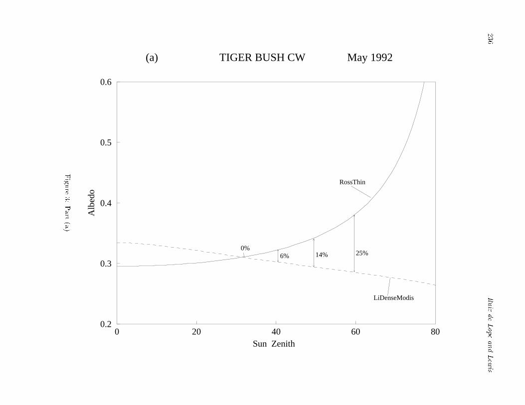
236
RuizdeLope
andLew
is
0 20 40 60 80Sun Zenith
0.2
0.3
0.4
0.5
0.6A
lbed
o
(a) TIGER BUSH CW May 1992
RossThin
LiDenseModis
0%6% 14% 25%
Figu
re3:
Part
(a)
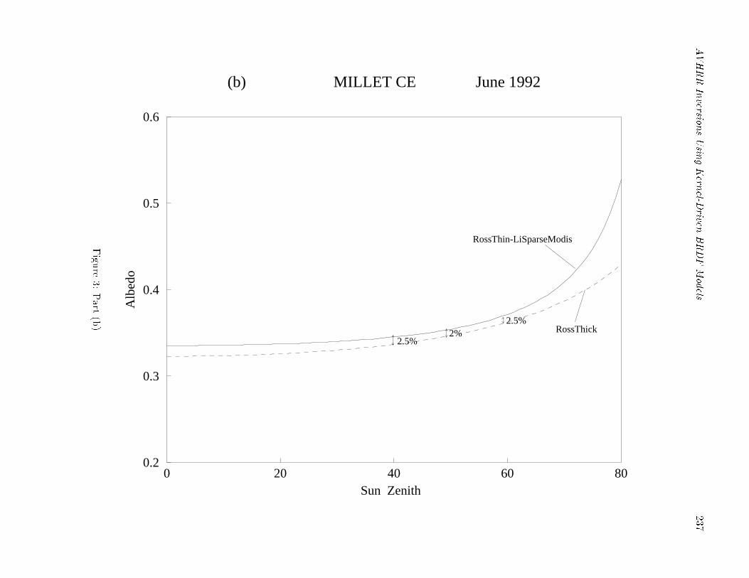
AVHRRInversio
nsUsin
gKern
el-Driven
BRDFModels
237
0 20 40 60 80Sun Zenith
0.2
0.3
0.4
0.5
0.6A
lbed
o
(b) MILLET CE June 1992
RossThick
RossThin-LiSparseModis
2.5%2%
2.5%
Figu
re3:
Part
(b)
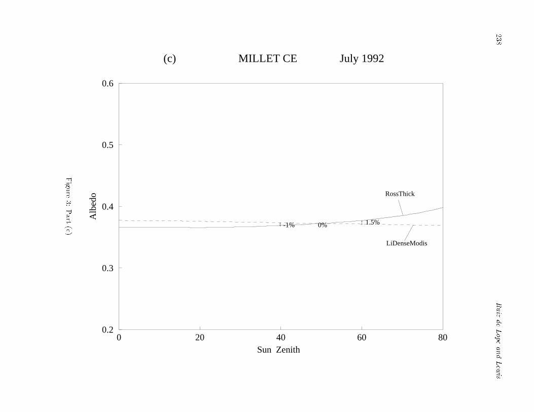
238
RuizdeLope
andLew
is
0 20 40 60 80Sun Zenith
0.2
0.3
0.4
0.5
0.6A
lbed
o
(c) MILLET CE July 1992
RossThick
LiDenseModis
-1% 0% 1.5%
Figu
re3:
Part
(c)

AVHRRInversio
nsUsin
gKern
el-Driven
BRDFModels
239
122 150 178 206 234 262 290day
0.000
0.005
0.010
0.015
0.020
0.025
0.030
0.035
0.040R
MSE
(A
VH
RR
Ban
d 1)
RossThinRossThickLiSparseModisLiDenseModisRossThin-LiSparseModisRossThin-LiDenseModisRossThick-LiSparseModisRossThick-LiDenseModis
Figu
re4:
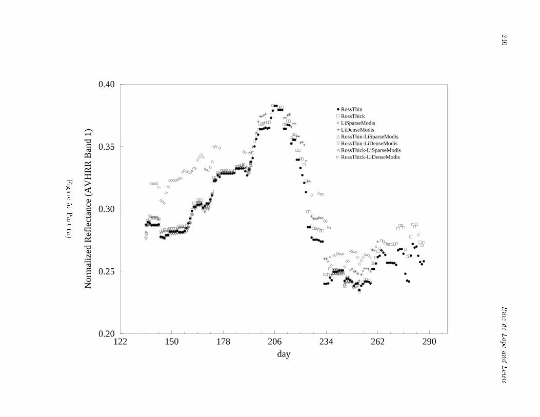
240
RuizdeLope
andLew
is
122 150 178 206 234 262 290day
0.20
0.25
0.30
0.35
0.40N
orm
aliz
ed R
efle
ctan
ce (
AV
HR
R B
and
1)
RossThinRossThickLiSparseModisLiDenseModisRossThin-LiSparseModisRossThin-LiDenseModisRossThick-LiSparseModisRossThick-LiDenseModis
Figu
re5:
Part
(a)
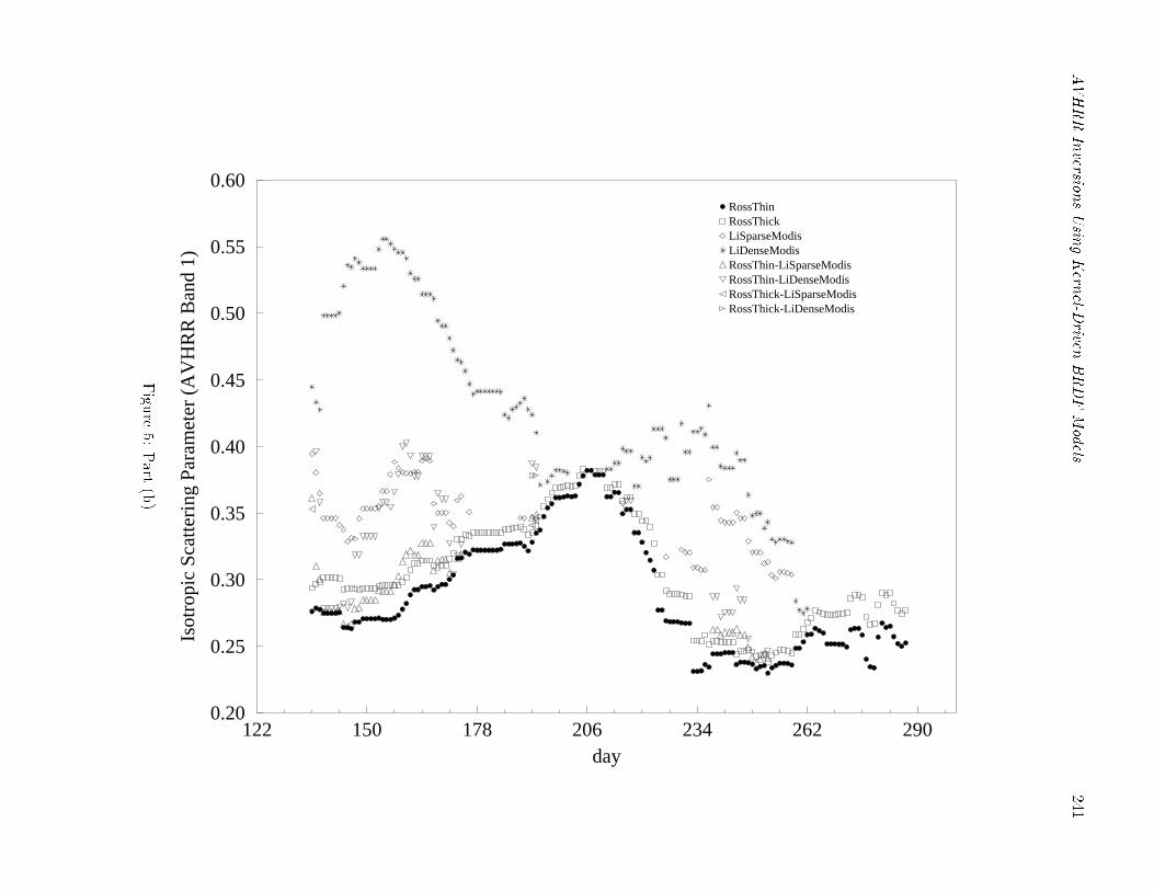
AVHRRInversio
nsUsin
gKern
el-Driven
BRDFModels
241
122 150 178 206 234 262 290day
0.20
0.25
0.30
0.35
0.40
0.45
0.50
0.55
0.60Is
otro
pic
Scat
teri
ng P
aram
eter
(A
VH
RR
Ban
d 1)
RossThinRossThickLiSparseModisLiDenseModisRossThin-LiSparseModisRossThin-LiDenseModisRossThick-LiSparseModisRossThick-LiDenseModis
Figu
re5:
Part
(b)

242
RuizdeLope
andLew
is
122 150 178 206 234 262 290day
0.0
0.2
0.4
0.6
0.8
1.0C
ompo
site
Nor
mal
ized
Ref
lect
ance
(A
VH
RR
Ban
d 1)
RossThinRossThickLiDenseModisRossThin-LiSparseModisRossThin-LiDenseModisRossThick-LiSparseModis
measured reflectance
modelled reflectance
RossThin RossThick
5% RMSE selecton
RMSE selection
Figu
re6:
Part
(a)
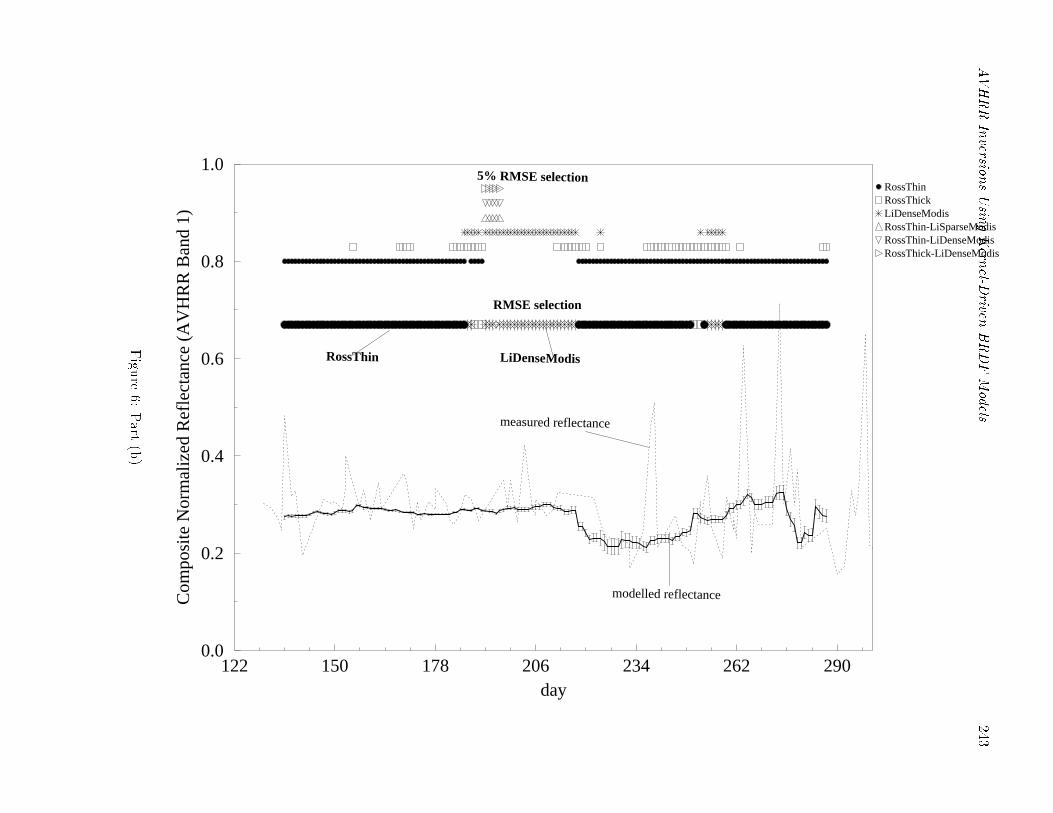
AVHRRInversio
nsUsin
gKern
el-Driven
BRDFModels
243
122 150 178 206 234 262 290day
0.0
0.2
0.4
0.6
0.8
1.0C
ompo
site
Nor
mal
ized
Ref
lect
ance
(A
VH
RR
Ban
d 1)
RossThinRossThickLiDenseModisRossThin-LiSparseModisRossThin-LiDenseModisRossThick-LiDenseModis
measured reflectance
modelled reflectance
RossThin LiDenseModis
5% RMSE selection
RMSE selection
Figu
re6:
Part
(b)

244 Ruiz de Lope and Lewis
APPENDIX J:
ESTIMATING LAND SURFACE ALBEDO IN THE HAPEX-SAHEL
SOUTHERN SUPER-SITE: INVERSION OF TWO BRDF MODELS
AGAINST MULTIPLE ANGLE ASAS IMAGES (SUMMARY OF A
PAPER BY BARNSLEY ET AL.)
AVHRR Inversions Using Kernel-Driven BRDF Models 245
Estimating Land Surface Albedo in the HAPEX-Sahel Southern Super-Site: Inversion
of Two BRDF Models Against Multiple Angle ASAS Images
(Summary of a Paper by Barnsley et al.)
Researchers at University College London recently applied the Roujean-RossThin kernel-driven semiempiricalBRDF model and the empirical modi�ed Walthall BRDF model to directional image data obtained for asemiarid region of West Africa near Niamay, Niger (Barnsley et al., 1996; Lewis et al., 1995). In this study,NASA's Advanced Solid-state Array Spectrometer (ASAS) (Irons et al., 1991) acquired image data froman aircraft platform over the HAPEX-Sahel west central, east central and southern super-sites on variousdates during September 3{17, 1992. The ASAS acquires images at ten sensor view angles during a singleoverpass | one at nadir and nine others at 15� increments between 75� forward and 60� aft of the aircraftplatform on which it is mounted. These images are recorded in 64 continuous narrow spectral wavebands inwavelengths ranging from the visible to the near-infrared. Spatial resolution is about 4 m. Data processinginvolved manipulating the multiple{view{angle and multiple ight{line ASAS image data in four steps: (i)geometric registration; (ii) radiometric correction; (iii) atmospheric correction; and (iv) estimation of thesurface (spectral) BRDF and albedo through BRDF model inversion.
Geometric registration of the multiple-view-angle and multiple ight-line data was perhaps the mostproblematic task. Standard polynomial warping techniques are generally unable to cope with the very highfrequency, localized geometric distortions present in most airborne scanner images. Consequently, Barnsleyet al. (1996) used an automated image registration procedure based on \interest point" extraction andarea-based matching of small patches of image around each interest point (Allison et al. 1991, Allisonand Muller 1992) to de�ne an initial polynomial mapping followed by pixel patch-by-pixel patch (typically15 x 15 pixels) matching using adaptive least-squares image correlation (Otto and Chau, 1989). Thesetechniques are capable of registering multiple view-angle ASAS images to subpixel accuracy (<0.4 pixels)globally throughout the scene (Allison et al. 1994). In this case, each of the o�-nadir images was registeredto the nadir view. Radiometric correction was e�ected using gain values provided by NASA to convertthe instrument's raw DN values to spectral radiances. Atmospheric correction was applied by use of the 6Satmospheric correction code (Vermote et al. 1994) with atmospheric parameters drived from sun photometerdata (Brown de Colstoun et al., 1996).
With registered and corrected data at hand, the Walthall and Roujean models were inverted and �ttedto the data on a pixel-by-pixel basis (Barnsley et al., 1996). This allowed the construction of images of theweights associated with each term of each model. The nadir re ectance images in the blue and near-infraredbands have low contrast and appear noisy. In these bands, the models seem to be �tting noise rather thansignal.
In contrast, the green and red bands show a coherent scene structure. The �rst parameters from bothWalthall and Roujean models are strongly related to overall brightness and thus mimic the nadir re ectance.The second and third parameters of the Walthall model show little spatial structure, although some brightand dark spots seem to correlate well with particular patches in the nadir image. In contrast, the Roujeanmodel shows strong spatial structure in both the �rst and second parameters. The second parameter isthe weight of the geometric kernel, which seems to vary inversely with the �rst parameter. This indicatesthat the BRDF becomes more isotropic with increasing brightness, which is not unexpected if multiplescattering increases with brightness. The �ne texture in the images of the third parameter may be relatedto �ne errors in registration, rather than real changes in BRDF within the scene. Overall, the weight of thethird parameter is quite low, indicating that volume scattering is not important for these surfaces. Sincevegetation is quite sparse over most of the target area, this is not unreasonable. These results demonstratethat a pixel-by-pixel inversion of empirical/semiempirical models is possible, and that the model parametersvary systematically in a meaningful spatial pattern.
We present a selection of �gures from this study. Figure 1 shows the multiple-view angle imagery used

246 Ruiz de Lope and Lewis
registered to the nadir view and atmospherically corrected. Figure 2 shows spatial images of the retrievedBRDF model parameters, and of albedo, using the modi�ed Walthall model, Figure 5 the same using theRoujean-RossThin model that is similar to the Ambrals BRDF model. Figure 3 shows a sample �t in severalwave bands, Figures 4 and 6 the respective histograms os RMSEs found in the inversions carried out on apixel by pixel basis.

AVHRR Inversions Using Kernel-Driven BRDF Models 247
6045
3015
0-1
5-3
0-4
5
555nm 645.6nm 862nm
Figure 1: The multiple-view angle spectral bidirectional re ectance factor data sets used in the study. Eachof the imahes is 128 by 128 pixels in size and has been extracted from co-registered and atmosphericallycorrected full-scene ASAS data. The �gure shows the magnitude of the angular variations in detectedre ectance. The angles reported in this �gure are the nominal ASAS camera angles.

248RuizdeLopeandLewis
Band 15 (555nm)Band 24 (645.6nm)Band 45 (862nm)
’albedo’f
0f
1f
2
Figure2:Spatiallyreferenceddatasetsofthemodi�edWalthallBRDFmodelparametersandthederivedspectralalbedo.Thesedatahavebeenproducedbyinvertingthemodi�edWalthallmodelagainstthespectralbidirectionalre ectancefactordatashownintheprevious�gure.Note,inparticular,thespatialpatternsthatareevidentinthevaluesofthemodelparameters.Thesearecloselyrelatedtospatialvariationsinthelandcoverandareboradlymaintainedinthespectralalbedodata.

AVHRR Inversions Using Kernel-Driven BRDF Models 249
-45.
0-3
0.0
-15.
00.
015
.030
.045
.060
.00.
00
0.10
0.20
0.30
0.40
0.50
0.60
0.70
862
nm
645.
6 nm
555
nm
mod
elle
d
mea
sure
d
mod
elle
d
mea
sure
d
mod
elle
d
mea
sure
d
view
zen
ith a
ngle
/ de
gree
s
reflectance
Figure 3: Plot showing the �ts between the measured and the modelled spectral bidirectional re ectancefactor data for the modi�ed Walthall BRDF model.
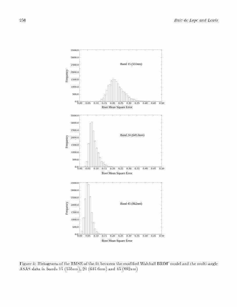
250 Ruiz de Lope and Lewis
Root Mean Square Error
Root Mean Square Error
Root Mean Square Error
Fre
quen
cyF
requ
ency
Fre
quen
cy
0.00 0.05 0.10 0.15 0.20 0.25 0.30 0.35 0.40 0.45 0.500.0
500.0
1000.0
1500.0
2000.0
2500.0
3000.0
3500.0
0.00 0.05 0.10 0.15 0.20 0.25 0.30 0.35 0.40 0.45 0.500.0
500.0
1000.0
1500.0
2000.0
2500.0
3000.0
3500.0
0.00 0.05 0.10 0.15 0.20 0.25 0.30 0.35 0.40 0.45 0.500.0
500.0
1000.0
1500.0
2000.0
2500.0
3000.0
3500.0
Band 15 (555nm)
Band 24 (645.6nm)
Band 45 (862nm)
Figure 4: Histograms of the RMSE of the �t between the modi�ed Walthall BRDF model and the multi-angleASAS data in bands 15 (555nm), 24 (645.6nm) and 45 (892nm).
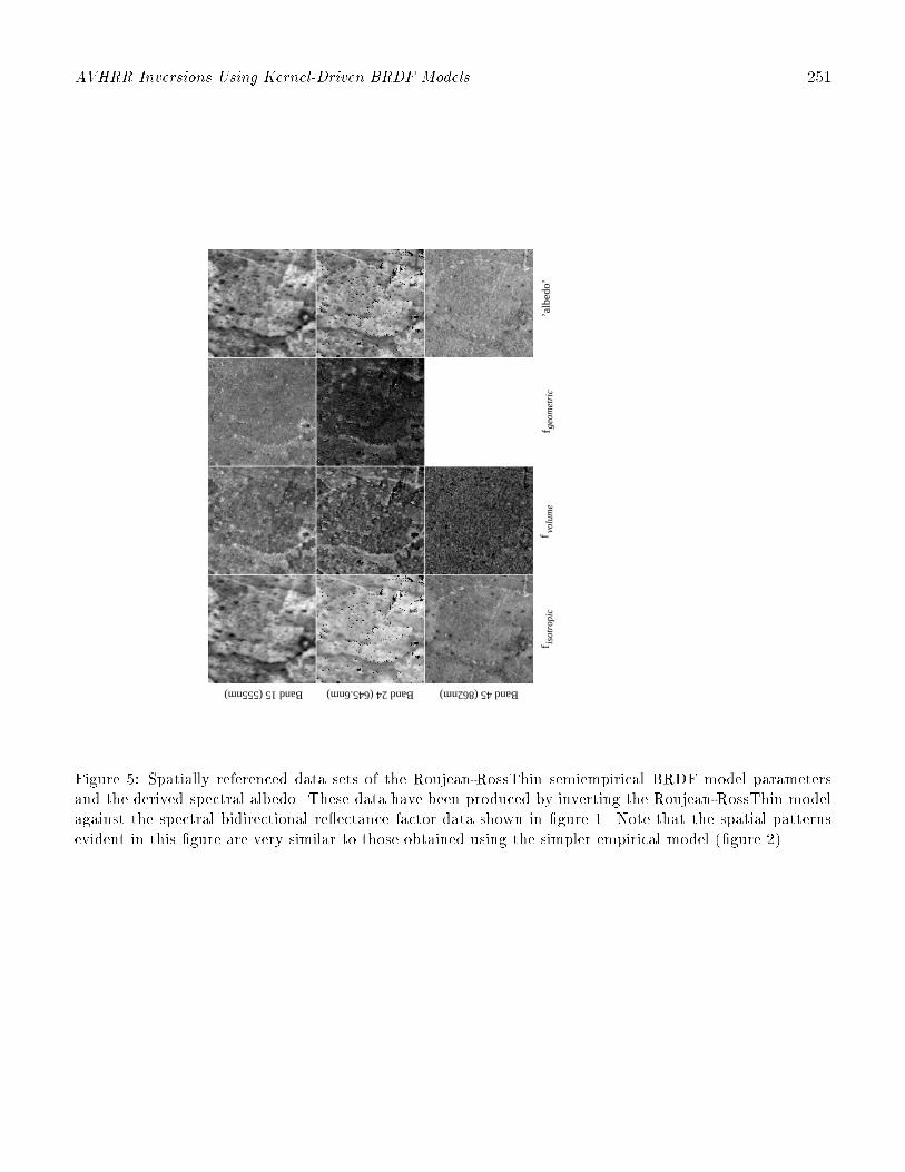
AVHRR Inversions Using Kernel-Driven BRDF Models 251
Band 15 (555nm) Band 24 (645.6nm) Band 45 (862nm)
’alb
edo’
f iso
tro
pic
f volu
me
f ge
om
etr
ic
Figure 5: Spatially referenced data sets of the Roujean-RossThin semiempirical BRDF model parametersand the derived spectral albedo. These data have been produced by inverting the Roujean-RossThin modelagainst the spectral bidirectional re ectance factor data shown in �gure 1. Note that the spatial patternsevident in this �gure are very similar to those obtained using the simpler empirical model (�gure 2).
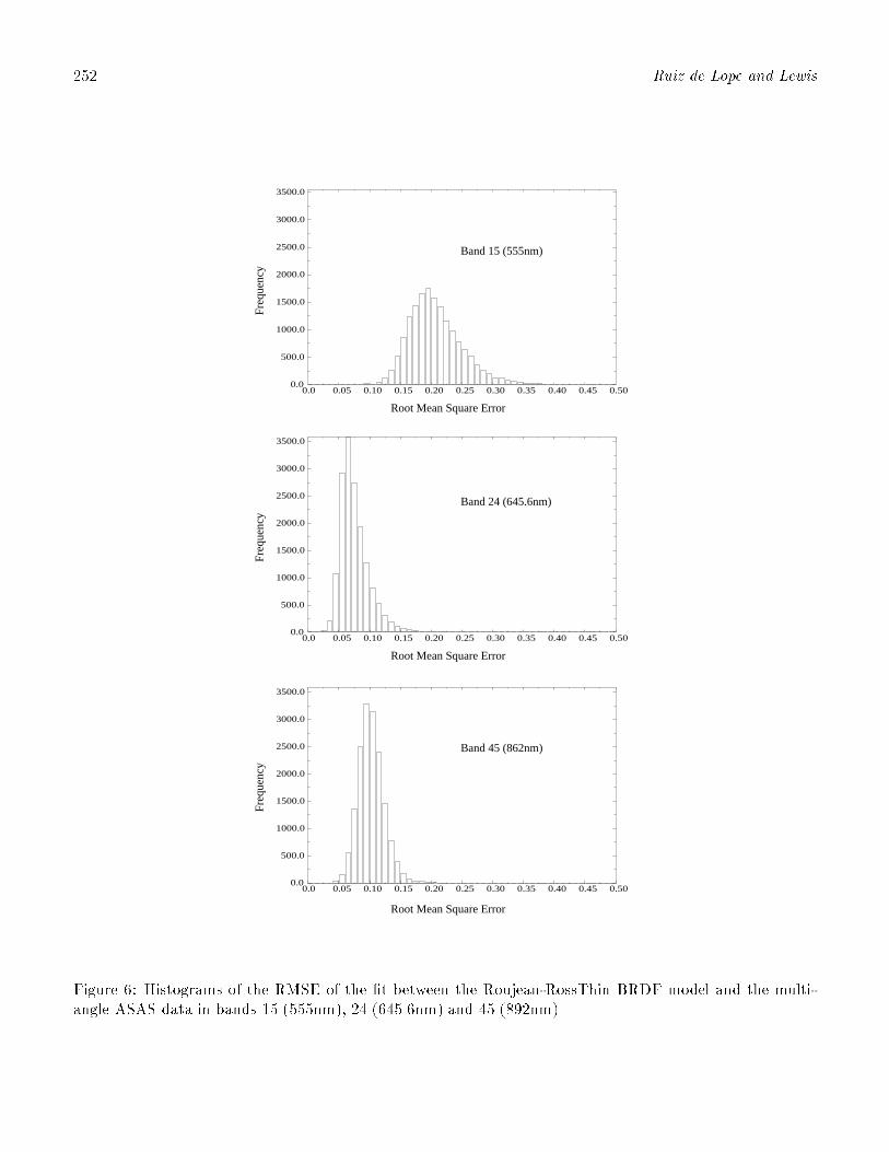
252 Ruiz de Lope and Lewis
0.0 0.05 0.10 0.15 0.20 0.25 0.30 0.35 0.40 0.45 0.500.0
500.0
1000.0
1500.0
2000.0
2500.0
3000.0
3500.0
0.0 0.05 0.10 0.15 0.20 0.25 0.30 0.35 0.40 0.45 0.500.0
500.0
1000.0
1500.0
2000.0
2500.0
3000.0
3500.0
0.0 0.05 0.10 0.15 0.20 0.25 0.30 0.35 0.40 0.45 0.500.0
500.0
1000.0
1500.0
2000.0
2500.0
3000.0
3500.0
Root Mean Square Error
Root Mean Square Error
Root Mean Square Error
Fre
quen
cyF
requ
ency
Fre
quen
cy Band 15 (555nm)
Band 24 (645.6nm)
Band 45 (862nm)
Figure 6: Histograms of the RMSE of the �t between the Roujean-RossThin BRDF model and the multi-angle ASAS data in bands 15 (555nm), 24 (645.6nm) and 45 (892nm).