Surface BRDF estimation from an aircraft compared to MODIS and ...

Surface BRDF estimation from an aircraft compared

to MODIS and ground estimates at the Southern

Great Plains site

Kirk D. Knobelspiesse,1 Brian Cairns,1,2 Beat Schmid,3 Miguel O. Roman,4

and Crystal B. Schaaf 4

Received 4 March 2008; revised 10 July 2008; accepted 12 August 2008; published 21 October 2008.

[1] Surface albedo, which quantifies the amount of solar radiation reflected by theground, is an important component of climate models. However, it can be highlyheterogeneous, so obtaining adequate measurements are challenging. Globalmeasurements require orbital observations, such as those provided by the ModerateResolution Imaging Spectroradiometer (MODIS). Satellites estimate the surfacebidirectional reflectance distribution function (BRDF), a surface inherent opticalproperty, by correcting observed radiances for atmospheric effects and accumulatingmeasurements at many viewing and solar geometries. The BRDF is then used to estimatealbedo, an apparent optical property utilized by climate models. Satellite observations areoften validated with ground radiometer measurements. However, spatial and temporalsampling differences mean that direct comparisons are subject to substantial uncertainties.We attempt to bridge the resolution gap using an airborne radiometer, the ResearchScanning Polarimeter (RSP). RSP was flown at low altitude in the vicinity of theDepartment of Energy’s Southern Great Plains Central Facility (SGP CF) in Oklahomaduring the Aerosol Lidar Validation Experiment (ALIVE) in September, 2005. The RSP’sscanning radiometers estimate the BRDF in seconds, rather than days required by MODIS,and utilize the Ames Airborne Tracking Sunphotometer (AATS-14) for atmosphericcorrection. Our comparison indicates that surface albedo estimates from RSP and MODISagree with Best Estimate Radiation Flux (BEFLUX) ground radiometer observationsat the SGP CF. Since the RSP is an airborne prototype of the Aerosol Polarimetery Sensor(APS), due to be launched into orbit in 2009, these techniques could form the basisfor routine BRDF validation.

Citation: Knobelspiesse, K. D., B. Cairns, B. Schmid, M. O. Roman, and C. B. Schaaf (2008), Surface BRDF estimation from an

aircraft compared to MODIS and ground estimates at the Southern Great Plains site, J. Geophys. Res., 113, D20105,

doi:10.1029/2008JD010062.

1. Introduction

[2] A proper understanding of surface albedo has been apriority of the remote sensing community since its origins.Besides providing information about the nature of thesurface itself, remote-sensing retrievals of atmosphericproperties must often account for the effects of the surfacereflectance. Albedo is also an important determinant ofwhere radiation is absorbed in climate models, yet it isspatially and temporally heterogeneous, and thus difficult to

include realistically in those models. In addition, anthropo-genic surface albedo changes can alter the global climate,but quantification of this process is dependent upon the datathat are used by models [Myhre and Myhre, 2003]. Globalalbedo estimates from sensors on satellite platforms are nowbeing compiled into climatologies appropriate for modeling[Lucht et al., 2000b; Schaaf et al., 2002; Luo et al., 2005]. Itis important, then, to verify the validity and accuracy ofthese global albedo products, and to identify any features ofthese products that would improve the reality of globalmodels without introducing unnecessary complexity.[3] Albedo is complex and highly variable. It is a

function of the surface material and its topography, whichis spatially and temporally heterogeneous, and the angle atwhich the surface is illuminated and observed. Low earthorbit satellite platforms with instruments such as the Mod-erate-Resolution Imaging Spectrometer (MODIS) and theMulti-angle Imaging SpectroRadiometer (MISR), as well asinstruments on geostationary satellites [Martonchik et al.,

JOURNAL OF GEOPHYSICAL RESEARCH, VOL. 113, D20105, doi:10.1029/2008JD010062, 2008ClickHere

for

FullArticle

1Department of Applied Physics and Applied Mathematics, ColumbiaUniversity, New York, New York, USA.

2NASA Goddard Institute for Space Studies, New York, New York,USA.

3Atmospheric Science and Global Change Division, Pacific NorthwestNational Laboratory, Richland, Washington, USA.

4Department of Geography and Environment, Center for RemoteSensing, Boston University, Boston, Massachusetts, USA.

Copyright 2008 by the American Geophysical Union.0148-0227/08/2008JD010062$09.00

D20105 1 of 21

http://dx.doi.org/10.1029/2008JD010062

2002; Pinty et al., 2005] are well suited to buildingclimatologies for modeling purposes, as they have a spatialcoverage and measurement repeat cycle that is impossible toachieve from ground or aircraft measurements. However,significant analysis is required to reduce the apparent opticalproperties (AOP’s), as seen at a satellite, to inherent opticalproperties (IOP’s) suitable for use in a climate model.Surface AOP’s depend on the solar and viewing geometryand on the atmospheric state through extinction of the directsolar beam before and after it reaches the surface andscattering of radiation on its way to and from the surface.For example, the measurement that is closest to a directestimate of albedo is the ratio of upwelling and downwel-ling fluxes, which is nonetheless an AOP since it dependson the atmospheric state. Since the atmospheric state varieswithin a climate model, the albedo must be described in anindependent manner as an IOP of the surface, that is thenused in a coupled calculation of the radiative transfer in thesurface-atmosphere system. The bidirectional reflectancedistribution function (BRDF) is an IOP that describes thereflectance of a surface when illuminated by an infinitesi-mally narrow beam of radiation and viewed through anequally infinitesimally narrow beam, and is a function of thegeometry of those two beams. Because of this, the BRDF is atheoretical property that can only be estimated [Schaepman-Strub et al., 2006]. Although several approaches have beendeveloped for the estimation of the BRDF over a wideangular range [Bruegge et al., 2000; Gatebe et al., 2003] amore common BRDF estimation approach is to fit anatmospherically corrected and geometrically variable set ofmeasurements to semi-empirical BRDF models [Engelsen etal., 1998; Lucht et al., 2000b]. The semi-empirical BRDFmodel can then be used to derive quantities that are notreadily observable, such as the variation of the albedo as afunction of solar zenith angle that is the function ofrelevance to most current climate models.[4] BRDF estimation from orbit is subject to several

hurdles. First, atmospheric effects must be removed, whichis complicated by multiple surface-atmosphere interactions.Second, a sufficient angular range of measurements must beaccumulated to provide a robust estimate of the semi-empirical BRDF model. In the case of fixed angle instru-ments such as MODIS, this accumulation requires severaldays, over which albedo characteristics may have changed.Multi-angle instruments such as MISR and the ResearchScanning Polarimeter (RSP, described below) sample amuch larger angular range nearly instantly, but this is at theexpense of spatial coverage. Third, in order to be effective forglobal evaluation of albedo, the semi-empirical BRDF mod-els must encompass a sufficient range of surface BRDF’s thattheir marginal integrals, such as albedo, are not biased by thechoice of model. Finally the data-model fitting methodshould be resistant to noise and methodological errors.[5] Because of the difficulties of BRDF estimation from

orbit, a robust validation effort is required to have sufficientconfidence to apply satellite derived climatologies to cli-mate models. As we noted above, ground radiometers makea measurement that is more directly related to albedo thanremote sensing measurements and they make that measure-ment as the solar zenith angle varies over the course of theday. Correctly modeling this energy input to the surface as afunction of solar zenith angle is important for general

circulation models. These measurements therefore providethe appropriate validation of the albedo derived fromsatellite, or aircraft measurements. However, care needs tobe taken when comparing with the ground radiometers toproperly account for the atmospheric state and the spectralsampling provided by the remote sensing measurements ascompared to the total fluxes measured at the surface.[6] Recently, there have been several efforts to compare

MODIS albedo products to ground radiometer data from theDepartment of Energy’s (DOE) Southern Great PlainsCentral Facility (SGP CF) in North-Central Oklahoma,USA [Luo et al., 2003; Yang, 2006; Schaaf et al., 2006],and to other ground radiometers [Liang et al., 2002; Jin etal., 2003]. For example, Yang [2006], compared parameter-izations of MODIS albedo [Liang et al., 2005; Wang et al.,2007] to Best Estimate Radiation Flux (BEFLUX) radio-meters [Shi and Long, 2002] and found some differences inthe shape of the albedo as a function of solar zenith angle.Since the the BEFLUX radiometers provide the directestimate of the energy input to the surface that we areinterested in for global applications it is important tounderstand whether these differences were due to inadequa-cies in the MODIS data itself, its parameterizations, orproblems with the comparison method.[7] Albedo data measured from aircraft utilizing multi-

angle and multi-spectral radiometers at the SGP CF offer thepossibility to investigate and resolve this issue. The AerosolLidar Validation Experiment (ALIVE) was in September of2005 in the vicinity of the SGP CF in northern Oklahoma.During ALIVE, a Jetstream-31 (J-31) turboprop aircraftflew several low altitude transects about 200 m above theSGP CF. The J-31 carried several instruments. The principalinstrument used here is the Research Scanning Polarimeter(RSP), a scanning polarimeter that is intended for aerosoland cloud research and is a prototype for the AerosolPolarimetery Sensor (APS). The APS is due to be launchedas part of the NASA Glory mission in 2008 [Mishchenko etal., 2007b]. RSP was flown at low altitudes to collect datafor the best possible estimate of the surface reflectance andBRDF.More details about the RSP are given in section 2.3.1.The Ames Airborne Tracking Sunphotometer (AATS-14)was also on the J-31. The AATS-14 is a fourteen spectralchannel sun tracking sun-photometer [Schmid et al., 2006]that provides accurate measurements of aerosol opticaldepth above the aircraft. The AATS-14 measurements ofaerosol above the aircraft in conjunction with measurementsfrom AErosol RObotic NETwork (AERONET) [Holben etal., 1998] ground-based sun-photometers allows us toperform an extremely accurate atmospheric correction ofthe RSP measurements. The atmospherically corrected RSPsurface measurements were fit to BRDF models from whichalbedos were derived and compared to MODIS andBEFLUX results. In addition, a land cover based approach,similar to that used in Liang et al. [2002], was used toevaluate the differences in spatial scale between MODIS,RSP and BEFLUX data.[8] The purpose of this paper is to evaluate the MODIS

BRDF retrievals that use semi-empirical kernel models toderive albedos and surface albedo parameterizations. Aspart of this evaluation, we also investigate previous valida-tion efforts at the SGP CF. RSP data provide a uniqueopportunity to bridge the spatial and temporal resolution

D20105 KNOBELSPIESSE ET AL.: AIRBORNE BRDF ESTIMATION AT THE SGP CF

2 of 21

D20105

differences between MODIS and ground radiometers in awell characterized atmospheric regime at the SGP CF.

2. Background

2.1. Albedo, BRDF, and Other Definitions

[9] Instruments observe many forms of what we callreflectance, which can have a somewhat complicated andambiguous terminology. We use nomenclature of Nicodemuset al. [1977], reviewed in Schaepman-Strub et al. [2006],which is briefly described here.[10] Reflectance, as it is most generally described, is the

ratio of radiant exitance from a surface to the irradiance, E,incident upon that surface. Both radiant exitance andirradiance have units of [W m�2], so reflectance, r, isunitless, and is constrained to the interval [0, 1]. Thereflectance factor, R, is the ratio of the radiant exitancefrom a surface to the radiant exitance leaving a perfectlyreflective, Lambertian (isotropic) surface under the sameirradiance. Occasionally, such as the case of strong forwardreflectance, the reflectance factor can exceed one. Both arefunctions of solar zenith angle, qs, view zenith angle, qv,solar azimuth angle, fs, view azimuth angle fv, and wave-length, l. We define wavelength for the narrow bandinstruments of interest here (RSP and MODIS) as the solarspectrum weighted center, L, of the spectral band of aparticular instrument.[11] The bidirectional reflectance distribution function

(BRDF) describes the scattering of a parallel beam ofincident light from one direction into another direction,defined as the ratio of the radiance observed through aninfinitesimally small solid angle cone to the irradianceilluminating that surface within an infinitesimal solid angle.

BRDF qs; qv;fs;fv;lð Þ ¼ dL qs; qv;fs;fv;lð ÞdE qs;f;lð Þ sr�1

� �ð1Þ

[12] The radiance, L, is the quantity of radiant flux perunit solid angle per unit wavelength and has units of[W m�2 sr�1]. The BRDF is an inherent optical property(IOP) and thus represents the intrinsic properties of thesurface. Since it is defined with infinitesimal quantities itcan not be directly measured. Its estimation, however, isimportant since apparent optical properties (AOP’s) can bederived from the BRDF in a consistent fashion appropriatefor validation. Moreover, given the typical scale of angularBRDF variations, it can be sampled and accurately estimated.[13] Schaepman-Strub et al. [2006] cites several AOP’s

that can be derived from the BRDF, but we use only two.The directional-hemispherical reflectance (DHR), called the‘‘black-sky’’ albedo in MODIS terminology, is the viewgeometry integrated, total radiant exitance when the surfaceis irradiated by a plane parallel beam. This is also known asthe planetary albedo in the astronomical literature.

DHR qs;fs;lð Þ ¼Z 2p

0

Z p2

0

BRDF qs; qv;fs;fv;lð Þ cos qvð Þ

� sin qvð Þdqvdfv ð2Þ

[14] Many publications assume DHR is independent ofthe solar azimuth angle (fs) which is the case if the BRDFonly depends on the difference between view and solarazimuth angles. If surface properties have no preferreddirection this is a reasonable assumption. In our case incentral Oklahoma, many of the surfaces are plowed fields orotherwise human influenced, so the DHR will not neces-sarily be invariant with respect to solar azimuth angle andthe BRDF will depend on both the view and solar azimuthangles independently. The magnitude of this azimuth angledependence is unknown. To maintain consistency withprevious literature and MODIS and BEFLUX products,we assume solar azimuth angle independence, but commentfurther on this issue in section 4.5.[15] Another albedo related quantity is the bihemispher-

ical reflectance (BHR), which represents the solar and viewgeometry integration of the BRDF (or the solar geometryintegration of the DHR). When the solar downwelling isassumed isotropic, BHR is the ‘‘white-sky’’ albedo inMODIS terminology. This is also known as the sphericalalbedo in the astronomical literature.

BHR lð Þ ¼Z p

2

0

Z 2p

0

Z p2

0

Z 2p

0

BRDF qs; qv;fs;fv;lð Þ

� cos qvð Þ sin qvð Þ cos qsð Þ sin qsð Þdqvdfvdqsdfs ð3Þ

[16] A function that we will define is the normalized DHR(nDHR). Many climate models assume that the shape of theDHR is spectrally invariant, and thus take as inputs thatshape and some scaling factor as a function of wavelengthand surface type. The nDHR is defined to be

nDHR qsð Þ ¼ DHR qs;lð ÞDHR 60�;lð Þ ð4Þ

[17] The nDHR will be used to compare different albedorelated measurements and to provide a direct comparisonwith the previous work of Yang [2006].

2.2. Ross-Li BRDF Kernel Models

[18] The BRDF is a theoretical parameter impossible tomeasure directly, even with the large number of view anglesavailable with the RSP. BRDF estimation is aided with theuse of surface reflectance models, where available measure-ments are fit with a combination of kernels, each represent-ing the geometric reflectance behavior a particular surfacetype. In this work, we use the kernel models employed inMODIS BRDF products, as described in Lucht et al.[2000b], and hereafter referred to as the Ross-Li BRDFmodel. Previous work has identified these kernels as pro-viding a robust and efficient framework for BRDF estima-tion [Schaaf et al., 2002] on a global scale, even when onlya limited geometric range of measurements are available.Our assessment of the use of these particular kernels here istherefore limited to how well they represent the denseangular sampling of the RSP measurements. An assessmentof the BRDF model validity for use in the evaluation of thesurface albedo in global climate models is provided bycomparisons to BEFLUX data.


3 of 21

D20105

[19] The Ross-Li BRDF model decomposes surface re-flectance into three types of scattering, and combines themin the following form:

BRDF qs; qv;f;lð Þ ’ R qs; qv;f;Lð Þ¼ fiso Lð Þ þ fvol Lð ÞKvol qs; qv;fð Þþ fgeo Lð ÞKgeo qs; qv;fð Þ ð5Þ

where Kvol and Kgeo are the volumetric and geometricscattering kernels, respectively, and fiso, fvol and fgeo, are theisotropic, volumetric and geometric kernel scaling para-meters.f is the relative view-sun azimuth angle (f =fv�fs).In practice, an optimization is used to find the best kernelscaling parameters (f) to a set of measured reflectances (R).The result is an estimation of the BRDF.[20] The first scaling parameter, fiso, represents isotropic

scattering, which has no dependence on incidence or viewangle and thus does not have a geometrically dependentkernel. Volumetric scattering represents the scattering with-in a dense vegetation canopy, and is based on a radiativetransfer approximation of single scattering due to small,uniformly distributed and non-absorbing leaves. The angu-lar behavior of this kernel is to have a minimum near thebackscatter direction and bright limbs. As described inRoujean et al. [1992] and Ross [1981], the volumetrickernel, normalized to zero for qv = qs = 0, is:

Kvol ¼p=2� xð Þ cos x þ sin x

cos qs þ cos qv� p

4ð6Þ

where x is the scattering angle, defined to be cos x = cos qvcos qs + sin qv sin qs cos f.[21] Geometric scattering represents surfaces with larger

gaps between objects, and thus accounts for self shadowing.The angular behavior of this kernel is therefore to have amaximum at backscattering where there are no shadows.Kgeo is based on the work of Wanner et al. [1995] and Liand Strahler [1992], but is used in the reciprocal form givenin [Lucht et al., 2000a]. This reciprocal form, in the specialcase that the ratio of the height of the tree at the center of thecrown to the vertical crown radius (h/b in Luo et al. [2005])is two and the ratio of the vertical crown radius to thehorizontal crown radius is one (spherical, or compactcrowns, b/r in Luo et al. [2005]) as is used in the MODISdata processing, is

Kgeo ¼ O qs; qv;fð Þ � sec qs � sec qv þ1

21þ cos xð Þ sec qs sec qv

O ¼ 1

pt � sin t cos tð Þ sec qs þ sec qvð Þ

cos t ¼

ffiffiffiffiffiffiffiffiffiffiffiffiffiffiffiffiffiffiffiffiffiffiffiffiffiffiffiffiffiffiffiffiffiffiffiffiffiffiffiffiffiffiffiffiffiffiffiffiffiD2 þ tan qs tan qv sinfð Þ2

qsec qs þ sec qv

D ¼ffiffiffiffiffiffiffiffiffiffiffiffiffiffiffiffiffiffiffiffiffiffiffiffiffiffiffiffiffiffiffiffiffiffiffiffiffiffiffiffiffiffiffiffiffiffiffiffiffiffiffiffiffiffiffiffiffiffiffiffiffiffiffiffiffiffiffiffiffiffiffiffiffitan2 qs þ tan2 qv � 2 tan qs tan qv cosf

pð7Þ

2.3. Instrument Description

2.3.1. RSP[22] The Research Scanning Polarimeter is an airborne

prototype for the Aerosol Polarimetery Sensor (APS), due tobe launched in 2008 as part of the NASA Glory Project

[Mishchenko et al., 2007b]. The main goals of RSP/APS areto retrieve a complete suite of aerosol and cloud micro-physical parameters together with the vertical distributionand integrated number concentration of particles from orbit[Mishchenko et al., 2004, 2007a]. The RSP has nine opticalchannels with center wavelengths of 410, 470, 555, 670,865, 960, 1590, 1880 and 2250 nm. This work utilizes all ofthese bands except for the 960 and 1880 nm channels,which are used to estimate water vapor column amounts anddetect thin cirrus clouds respectively. Details about the RSP/APS aerosol retrieval using polarimetry can be found inCairns [2003] and Chowdhary et al. [2002].[23] In addition to measuring the polarized reflectance

beneath the RSP with each scan, the instrument alsomeasures the total (unpolarized) reflectance. While thisinformation is not currently utilized to retrieve aerosolparameters over land, it is useful to independently validatesurface albedo values retrieved by MODIS or other orbitalplatforms. Each RSP scan begins about 60� forward of nadirin the direction of aircraft motion, and samples at 0.8�intervals to about 60� aft of nadir. Thus each scan containsabout 150 instantaneous samples at a variety of sensorviewing geometries. A BRDF estimation is therefore pos-sible with a larger set of surface anisotropic reflectances, asopposed to fixed viewing angle instruments, such asMODIS, which require an accumulation of observationsover several days (16 in case of the MODIS MCD43Bproduct) before the BRDF can be estimated [Lucht et al.,2000b]. The instantaneous field of view (IFOV) of the RSPis fourteen milliradians, which corresponds to a 2.8 mground pixel size assuming an altitude of 200m above theground. RSP measurements were made over a period of twoweeks during the ALIVE campaign in September, 2005.Two flights, labeled JRF03 and JRF04 in ALIVE terminol-ogy, were on September 16th and were chosen for thisanalysis for the clear, cloudless conditions at that time, andthe low altitude segments of those flights that were made inthe vicinity of the SGP CF. More details about dataselection for the RSP are in section 3.1.1.[24] The RSP performed two types of flights during

ALIVE. The first type was to collect data at an altitudeabove the majority of the atmospheric aerosols, generally4–5 km above ground on September 16th, 2005. Anindication of the required altitude was provided by theAATS-14, see section 2.3.2. The atmospheric state isdetermined from these measurements, which are then ap-plied in the atmospheric correction of data from the secondtype of measurements, collected at as low an altitude aspossible. These low altitude data (about 200 m above theground) were used for BRDF estimation. The low altitudewas key to minimize the atmospheric effect between theRSP and the ground, maximize spatial resolution, andminimize the effect of aircraft motion on efforts to combineviews from different scans into a multi-angle observation ofa single surface location.2.3.2. AATS-14, Ancillary Data, and the RadiativeTransfer Model[25] RSP surface reflectance retrievals utilized several

types of ancillary data. These data were used in theatmospheric correction of the observed radiances to removeatmospheric effects. An important component of the RSPatmospheric correction was the Ames Airborne Tracking


4 of 21

D20105

Sunphotometer (AATS-14), co-located on the J-31 with theRSP. The AATS-14 provides a continuous record of aerosoloptical depth above the aircraft in fourteen channels from354 to 2139 nm [Schmid et al., 2006]. These data were usedin three ways. First, AATS-14 measured the vertical extentand distribution of aerosols during aircraft ascent anddescent. This identified the required altitude for ‘‘highaltitude’’ RSP measurements where aerosol parameters areretrieved. Second, information about the aerosols, such asthe nature of their vertical distribution and the presence ofvery large coarse mode aerosols helped constrain the RSPaerosol retrievals. Finally, AATS-14 measurements during‘‘low altitude’’ flights identified where in the aerosol layerthe aircraft was located. This is particularly useful whenAATS-14 data are compared to AERONET ground sun-photometers, which thus indicates the aerosol optical depthbetween the instrument and the ground.[26] Several other sources of data provide ancillary infor-

mation necessary to remove the effect of various compo-nents of the atmosphere. Ozone absorption, which isgreatest in the 470 and 555 nm bands, is based on the daily1� 1� values from the Total Ozone Mapping Spectrometer(TOMS) [McPeters and Center, 1998]. Absorption due toNO2, greatest at the shortest wavelength channels, is esti-mated using Scanning Imaging Absorption Spectrometerfor Atmospheric Chartography (SCIAMACHY) data[Bovensmann et al., 1999]. Water vapor content wasmeasured by the Microwave Radiometer (MWR) locatedat the SGP CF [Morris, 2006].2.3.3. MODIS[27] The MODerate resolution Imaging SpectroRadiom-

eter (MODIS) is a multispectral remote sensing satellite in apolar orbit. There are actually two MODIS instruments, onthe morning equator crossing NASA Terra (EOS-AM) andafternoon equator crossing NASA Aqua (EOS-PM) space-craft. Terra was launched in 1999, and Aqua in 2002. SinceALIVE was in September of 2005, we used a combinationof data from both instruments. MODIS produces a largenumber of atmospheric and surface products, but we havefocused our attention on the surface albedo retrievals,referred to as product ID MCD43 in MODIS terminology.We used the ‘‘collection five’’ processing version, whichhas a 500 m ground resolution. MODIS measures surfacereflectance at a single view zenith angle with each scan, soalbedos are determined by fitting several days worth of data(containing a variety of view and solar zenith angles) to aset of BRDF models (described in section 2.2). The meth-odology for doing so is described in Lucht et al. [2000b]and Strahler et al. [1999], and first operational results arepresented in Schaaf et al. [2002].[28] A number of efforts have been made to validate

MODIS albedo products. Often, this takes the form of acomparison of satellite MODIS results to measurementsfrom ground based radiometers. However, care must betaken to ensure that this comparison accounts for the spatialand temporal resolution differences between remote sensinginstruments and ground radiometers. MODIS (and RSP)measurements represent a combination of all reflectanceswithin a pixel, which may include a variety of surface types,while ground radiometers measure albedo with a smallerspatial scale that is dependent on the height of the tower onwhich the upwelling flux measurement is made and the

observed portion of the radiative spectrum. In addition, themulti-day data aggregation required with the MODIS data-set could be problematic if that aggregation period includeschanges to surface properties. It is therefore difficult todetermine if comparisons represent purely instrumentaldifferences, or are also affected by resolution.[29] Prior to the launch of Terra, Lucht et al. [2000a]

attempted to validate the BRDF kernel fitting method bycomparing ground radiometer measurements to reflectancesfrom other remote sensing platforms. Spatial resolutiondifferences were controlled by doing this comparison in aregion of low albedo variability (grass and scrubland inNew Mexico, USA), and BHR results were close enough foraccurate climate modeling. Liang et al. [2002] validatedMODIS albedo by ‘‘upscaling’’ ground radiometer meas-urements from an agricultural region in Maryland, USA.They report less than 5% absolute error. Jin et al. [2003]compared MODIS albedo to field measurements from theSurface Radiation Budget Network (SURFRAD) and foundresults that met an accuracy requirement of 0.02 for meas-urements between April and September. Winter measure-ments failed to meet requirements, most likely due to theinfluence of rapid albedo changes from snow. With thelaunch of Aqua, Salomon et al. [2006] updated MODISalbedo validation for the combined Terra/Aqua productusing SURFRAD and radiometers at the SGP CF. He foundthat, while wintertime albedo remain uncertain as describedin Jin et al. [2003], overall coverage improved while totaldata averages remained consistent with previous results.[30] Validation efforts described above are generally

restricted to comparisons of BHR, whereas for climatemodeling a DHR parameterization is also needed. Severalattempts have been made to parameterize MODIS results forapplication in climate models. Liang et al. [2005] created aparameterization using DHR and BHR from MODIS, soilmoisture from the North American and Global Land DataAssimilation System (LDAS), fractional vegetation cover,and leaf and stem area index. Wang et al. [2007] used asimplification of MODIS DHR and a measure of vegetationtype to create another type of parameterization. Yang [2006]investigated the validity of these parameterizations of DHRby comparing them to BEFLUX radiometer values at theSGP CF. While both parameterizations agreed well witheach other at this site, Yang [2006] found differences incomparison to ground radiometers. Parameterization valueswere much smaller than BEFLUX values at high solarzenith angles and larger than BEFLUX values at very smallsolar zenith angles. While the former is perhaps to beexpected considering the lack of MODIS data at high solarzenith angles, the latter is unexpected and troubling. Ourwork was initiated as an attempt to further investigate andpossibly resolve the differences found in Yang [2006] withregards to how well MODIS surface albedo data productscan predict surface albedo.2.3.4. BEFLUX[31] Ground radiometer data were supplied by the Best

Estimate Flux (BEFLUX) value-added procedure (VAP),which is created from several radiometers at the Departmentof Energy’s Atmospheric Radiation Measurement (ARM)Southern Great Plains Central Facility (SGP CF). BEFLUXradiometers measure diffuse and total hemisphericaldownwelling irradiance and total hemispherical upwelling


5 of 21

D20105

irradiance in one minute intervals [Shi and Long, 2002].These values were combined according to the methodologyof Yang [2006] to compute a BHR and DHR representingthe rural pasture at the SGP CF in North-central Oklahoma,USA. This was done in two steps. First, the BHR for theentire month of September, 2007 was determined by findingthe average ratio of total upwelling to total downwellingirradiance from cloudy measurements. These cloudy meas-urements were identified by the ratio of direct to totalhemispherical downwelling irradiance. The BHR was thenutilized to find the DHR on the day of the measurement.

3. Method

3.1. RSP Data Preparation

3.1.1. Data Selection[32] The Aerosol LIdar Validation Experiment (ALIVE)

was a field campaign performed in North-central Oklahomain September of 2005. This is the location of the SouthernGreat Plains Central Facility (SGP CF) of the AtmosphericRadiation Measurement (ARM) Program (Department ofEnergy). While the primary goals of the ALIVE campaignwere not to investigate RSP surface characterization, theproximity to the suite of ground based instruments at theSGP site, simultaneous measurements of the aerosol profilefrom AATS-14, and a series of low altitude flights, providean ideal data-set with which to investigate the surfacecharacterization.[33] Several short, low altitude flight segments were

made in the vicinity of the SGP site, typically preceded orfollowed by a spiral maneuver used by the AATS-14 todetermine an aerosol optical thickness altitude profile.Surface characteristics were typical for the rural mid-westof the United States in the fall. The ground was relativelyflat, and covered by a patchwork of late-season crops, baresoil exposed by recent harvesting, and mixtures of trees andshrubs [Luo et al., 2003]. There are few buildings and theoccasional paved road.[34] Data from two flights were used. Table 1 presents

these flight times, along with geometry, aerosol and weatherconditions. Aerosol optical thickness at 500nm from anAERONET Project [Holben et al., 1998] sun photometer atthe SGP site is also included to provide an understanding ofaerosol properties from that day.[35] In Table 1, the tags in the first row (JRFx) identify

the research flight. Start time for a data file within that flightis listed in UTC. Local time was five hours earlier. Scanswere selected from a particular data file so that they

included only low altitude, constant heading segments.Altitude is listed as meters above sea level. Ground heightat the SGP site is about 315 m, so flights had an aboveground height between 160 and 195 m. The (relative)azimuth is the instrument heading minus solar azimuth, indegrees. Aerosol optical thickness at 500 nm (ta) wasmeasured by the AERONET Project with a ground sunphotometer at the SGP site. Values from the time of flightare provided for comparison. AATS-14 optical thicknesswas measured on the J-31. Thus differences between AATS-14 and AERONET represent the optical thickness betweenthe aircraft and the ground, a value which is well within theAERONET and AATS-14 uncertainty. The last row containsa visual description of the cloud scenario from the instru-ment operator.[36] There were a total of twelve research flights as part

of ALIVE, but only flights JRF3 and JRF4, listed above,were suitable for BRDF estimation. JRF3 and JRF4 werethe only flights with low altitude segments when the skywas completely devoid of clouds. As we shall see later (seesection 3.1.3), some effort was put into determining thediffuse downwelling irradiance while estimating the BRDF.This determination is only accurate, with our models, forclear skies. Including the effects of clouds under partiallycloudy skies, even if implemented with a three dimensionalradiative transfer code, would introduce large uncertainties,as there is limited informational to specify the vertical andhorizontal cloud distribution.3.1.2. Classification and Mixed Pixel Removal[37] Before the Ross-Li BRDF models were fit to the

data, we separated it into similar classes, and performed ourfitting on each class individually. This was done to limit thedependence on data coverage differences from flight toflight, and also to facilitate comparisons with other lowerspatial resolution data sets. Prior to image classification,gaseous absorption effects were removed as describedabove, and a metric describing the amount of vegetation(a vegetation index, see Appendix B) was calculated foreach data point. Data were then split into ‘‘soil’’ and‘‘vegetation’’ classes and extreme vegetation index valueswere removed. Boundary or mixed surfaces were alsoremoved using an edge detection convolution kernel onthe spatial image of vegetation index. In addition, analyseswere performed on an ‘‘all’’ class which contains the entiredata-set except for data that were removed as part of thequality control process. For each of these classes the datawere then fit with the Ross-Li BRDF model.[38] Simple thresholding of the Aerosol Resistant Vege-

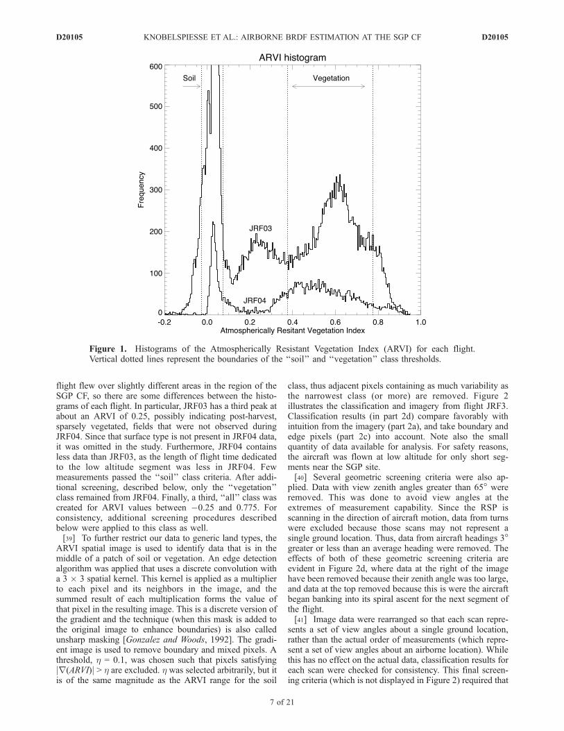
tation Index (ARVI, see Appendix B for details on how it iscomputed) was used to split the data into a ‘‘soil’’ and‘‘vegetation’’ class. ARVI values between �0.25 and 0.075were classified as ‘‘soil’’, while ARVI values between 0.375and 0.775 were classified as ‘‘vegetation’’. Such narrowARVI regions centered on the modes of each surface typewere chosen to avoid mixed pixel data and focus on theproperties of generic ‘‘soil’’ and ‘‘vegetation’’. Figure 1 is ahistogram of the ARVI for each flight. Peaks for bothclasses are pronounced, and vertical dashed lines show theregions used for each class. The histogram computed usingdifferent small segments of the view angle range (notpictured here) is similar to the one shown here indicatingan absence of significant BRDF effects on this index. Each

Table 1. Low Altitude ALIVE Flight Segments Used for Surface

Characterization

JRF3 JRF4

Date 09/16/2005 09/16/2005Start time, UTC 16:32:25 22:09:32Number of RSP scans 270 41J-31 Altitude above sea level 510 m 475 mRelative sensor-solar azimuth �45� 156�Solar zenith angle 43� 62�AERONET ta(l = 500 nm) 0.07 0.05AATS-14 ta(l = 499 nm) 0.06 0.05sky conditions clear clear


6 of 21

D20105

flight flew over slightly different areas in the region of theSGP CF, so there are some differences between the histo-grams of each flight. In particular, JRF03 has a third peak atabout an ARVI of 0.25, possibly indicating post-harvest,sparsely vegetated, fields that were not observed duringJRF04. Since that surface type is not present in JRF04 data,it was omitted in the study. Furthermore, JRF04 containsless data than JRF03, as the length of flight time dedicatedto the low altitude segment was less in JRF04. Fewmeasurements passed the ‘‘soil’’ class criteria. After addi-tional screening, described below, only the ‘‘vegetation’’class remained from JRF04. Finally, a third, ‘‘all’’ class wascreated for ARVI values between �0.25 and 0.775. Forconsistency, additional screening procedures describedbelow were applied to this class as well.[39] To further restrict our data to generic land types, the

ARVI spatial image is used to identify data that is in themiddle of a patch of soil or vegetation. An edge detectionalgorithm was applied that uses a discrete convolution witha 3 3 spatial kernel. This kernel is applied as a multiplierto each pixel and its neighbors in the image, and thesummed result of each multiplication forms the value ofthat pixel in the resulting image. This is a discrete version ofthe gradient and the technique (when this mask is added tothe original image to enhance boundaries) is also calledunsharp masking [Gonzalez and Woods, 1992]. The gradi-ent image is used to remove boundary and mixed pixels. Athreshold, h = 0.1, was chosen such that pixels satisfyingjr(ARVI)j > h are excluded. h was selected arbitrarily, but itis of the same magnitude as the ARVI range for the soil

class, thus adjacent pixels containing as much variability asthe narrowest class (or more) are removed. Figure 2illustrates the classification and imagery from flight JRF3.Classification results (in part 2d) compare favorably withintuition from the imagery (part 2a), and take boundary andedge pixels (part 2c) into account. Note also the smallquantity of data available for analysis. For safety reasons,the aircraft was flown at low altitude for only short seg-ments near the SGP site.[40] Several geometric screening criteria were also ap-

plied. Data with view zenith angles greater than 65� wereremoved. This was done to avoid view angles at theextremes of measurement capability. Since the RSP isscanning in the direction of aircraft motion, data from turnswere excluded because those scans may not represent asingle ground location. Thus, data from aircraft headings 3�greater or less than an average heading were removed. Theeffects of both of these geometric screening criteria areevident in Figure 2d, where data at the right of the imagehave been removed because their zenith angle was too large,and data at the top removed because this is were the aircraftbegan banking into its spiral ascent for the next segment ofthe flight.[41] Image data were rearranged so that each scan repre-

sents a set of view angles about a single ground location,rather than the actual order of measurements (which repre-sent a set of view angles about an airborne location). Whilethis has no effect on the actual data, classification results foreach scan were checked for consistency. This final screen-ing criteria (which is not displayed in Figure 2) required that

Figure 1. Histograms of the Atmospherically Resistant Vegetation Index (ARVI) for each flight.Vertical dotted lines represent the boundaries of the ‘‘soil’’ and ‘‘vegetation’’ class thresholds.


7 of 21

D20105

50% of the data in a scan must have passed all previousscreening criteria and were grouped into a single class. Theresult is a set of data that is of a consistent surface type overmost of the view angle range and that has had any outliermeasurements, which may represent noise, surface bound-ary or mixed pixel effects removed.3.1.3. Determination of Ground Reflectance and theDiffuse Effect[42] Measurement of ground reflectance from an aircraft

requires adequate compensation for atmospheric effects.During ALIVE, a high quality characterization of theatmospheric scattering was provided by the combinationof polarized RSP measurements (above the aerosol layer)with the vertical profile of aerosol optical thicknesses fromthe AATS-14. This cannot be used to determine the groundreflectance directly because of the multiple scattering thatoccurs between the atmosphere and the surface. The atmo-spheric correction is therefore performed using an iterativeprocess, where initial estimates of surface reflectance areadjusted until the surface-atmosphere scattering modelreproduces the reflectance measured by the RSP.[43] The atmospheric-surface model uses the doubling

and adding method [Lacis and Hansen, 1974; Hansen andTravis, 1974], and produces a reflectance to compare toRSP data, given aerosol and other atmospheric propertiestogether with solar and instrument geometry and kernel

values for the Ross-Li BRDF reflectance model. Theobserved reflectance can be separated into an atmosphericand a surface component:

ro qs; qv;f;lð Þ ¼ ra qs; qv;f;lð Þ þ S qs; qv;f;lð Þ ð8Þ

where ro is the reflectance at the altitude of theobservations, ra is the reflectance due to atmosphericscattering of radiance into the instrument field of viewwithout interacting with the surface (path radiance) and Sincludes all surface interaction terms. In what follows weare primarily interested in S and the correction for diffuseand multiple interaction terms, since we have an accurateand comprehensive characterization of the atmosphere fromhigh altitude RSP measurements that allows us to calculatera. We will differentiate between measurements and modelcalculations by using a caret for those quantities that aredirect observations. The surface interaction term, S, can becalculated using the expression

S qs; qv;f;lð Þ ¼t" qv;lð Þ þ T" lð Þ*� �

rg qs; qv;f;lð Þ t# qs;lð Þ þ *T# lð Þ

� �þ t" qv;lð Þ þ T" lð Þ*� �

S qs; qv;f;lð Þ*rg qs; qv;f;lð Þ� t# qs;lð Þ þ *T

# lð Þ� �

ð9Þ

Figure 2. Data from flight JRF03 was used to show (from left to right), (a) Ground reflectance, wherethe 670 nm band is displayed in the red channel, the 865 nm band in the green channel, and the 470 nmband in the blue channel, (b) Atmospherically Resistant Vegetation Index (ARVI), with the color bar atthe right, (c) gradient of ARVI, used to remove boundary and edge pixels with its color bar at the right,and (d) classification results, where red indicates ‘‘soil’’ type, green indicates ‘‘vegetation’’, and black areunclassified areas.


8 of 21

D20105

where rg is the surface reflectance, t is the direct solartransmittance, and T is the diffuse transmittance, with thearrows indicating whether they apply to transmission fromthe sun to the ground (#) or from the ground to theobservational altitude ("). The star symbol, *, indicates thatintegrations over zenith and azimuth are performed fordiffuse interactions. As is usually the case for scatteringproblems with no preferred azimuthal plane, that integrationis actually implemented using a Fourier decomposition andre-summation [Hovenier, 1971; Hansen and Travis, 1974;de Haan et al., 1987]. The function S is used in thecalculation of multiple surface atmosphere interaction termsand is given by the formula

S qs; qv;f;lð Þ ¼X1i¼1

rg qs; qv;f;lð Þ * ra? qs; qv;f;lð Þð Þi ð10Þ

where ra? is the reflectance of the atmosphere illuminatedfrom below. The implementation of this summation isdescribed in [Hovenier, 1971; Hansen and Travis, 1974; deHaan et al., 1987].[44] In equation (8), ro is measured by the RSP and

calculated with the doubling-adding model, while ra, t, Tand S are determined from the model based on the atmo-spheric state that is prescribed by AATS-14, AERONET andhigh altitude RSP data. The model includes the effects ofboth Rayleigh (molecular) and aerosol scattering. In order tofind an estimate of rg that has the effects of diffusetransmission and multiple surface-atmosphere scatteringremoved, we use the following iteration

rgpþ1 qs; qv;f;lð Þ ¼ S qs; qv;f;lð ÞSp qs; qv;f;lð Þ

" #rg;kp qs; qv;f;lð Þ

¼ gp qs; qv;f;lð Þrg;kp qs; qv;f;lð Þ ð11Þ

where p is the iteration index, rg,k is the kernel fit to thelatest estimate of surface reflectance and S is theobservation corrected for path radiance. We have implicitlydefined the function gp, which is the ratio of measurementto model S, to adjust the surface reflectance until the modelcalculated reflectance matches the observations. Thisiteration is similar to that introduced by Chahine [1968]for atmospheric sounding. The kernel fit to the reflectanceuses a least mean square estimate of the kernel coefficients,so the vector of kernel coefficients, f, is given by theexpression

fpþ1 ¼ K qvð ÞTK qvð Þh i�1

K qvð ÞT�

rgpþ1 qvð Þ ð12Þ

and the kernel estimate for the surface reflectance at theobserved viewing geometry is

rg;kpþ1 qvð Þ ¼ K qvð Þfpþ1 ð13Þ

with K being the 3 N reflectance kernel matrix formedfrom the isotropic, volumetric and geometric kernels (cf.equation (5)) and N is the number of view angles for thegiven viewing geometry. K and f depend on the same set ofwavelength (l) and other geometric parameters (qs, f), so

those subscripts are omitted from the above equations. Theiteration is initialized with the value

rg1 qs; qv;f;lð Þ ¼ S qs; qv;f;lð Þt" qvð Þt# qsð Þ ð14Þ

[45] In an atmosphere with no scattering this initial valuegives the atmospherically corrected surface reflectance, andno further iterations are therefore necessary. Otherwise,equations (11) through (13) are iterated until g is close tounity. If there is scattering in the atmosphere, we candetermine that g < 1 from equation (9) for the first step inthe iteration. This is a necessary condition for the conver-gence of this iteration [Twomey, 1977]. Convergence alsorequires that the matrix associated with the estimate of thekernel parameters is diagonally dominant (Dubovik andKing [2000], Appendix C). Since we are interested in theconvergence of the estimation of the weights associatedwith the kernels we define matrix M

Mjk ¼@ln rg;k qv;l

� �� @ln fj� �

!�1@ln S qv;l

� �� @ln fk½ � ð15Þ

where we use the convention that there is a summation overrepeated subscripts. The average degree of diagonaldominance of that matrix, dd, is

dd ¼Xi

Pi6¼j jMijjMii

ð16Þ

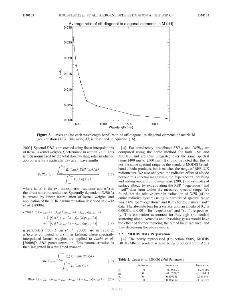
[46] As expected (see Figure 3), dd is largest at shortestwavelengths, where the effects of scattering are largest, andsmallest at the longer wavelengths, where the effects ofscattering are negligible.[47] The final iteration products are the kernel values of

the Ross-Li surface reflectance model. The iteration wasrepeated between 5–9 times for each band until the changein kernel values for each iteration was smaller than 10�5.3.1.4. Spectral to Broadband Albedo Computation[48] DHR and BHR, as calculated in the previous section,

represent surface properties in a set of narrow instrumentbands. Data from these narrow bands must be spectrallyinterpolated if they are to be compared to broadband groundradiometer data such as that from BEFLUX. In MODISproducts, this is done according to the methodology ofLiang [2001] and validated in Liang et al. [2003]. Liang[2001] used libraries of surface reflectance spectra andmodel simulations to create a set of coefficients that areapplied to scene albedo values to approximate a broadbandDHR or BHR. These coefficients are applied uniformlyacross the entire MODIS dataset. Our RSP-ALIVE datasetcomprises a single day with a well known atmosphericscenario. In this sense, we are fortunate in that we canutilize knowledge about the atmosphere in our broadbandalbedo computation, and we do so as follows.[49] Conversion of DHR(L, qs) to the broadband version

DHRbb(qs) involves the spectral integration of the DHRweighted by the downwelling solar irradiance. Irradiancesare computed using a hyperspectral version of the doublingand adding model applied in section 3.1.3 [Cairns et al.,


9 of 21

D20105

2003]. Spectral DHR’s are created using linear interpolationsof Ross-Li kernel weights, f, determined in section 3.1.3. Thisis then normalized by the total downwelling solar irradianceappropriate for a particular day at all wavelengths

DHRbb qsð Þ ¼

Z lmax

lmin

Eo lð Þt lð ÞDHR l; qsð ÞdlZ lmax

lmin

Eo lð Þt lð Þdlð17Þ

where Eo(l) is the exo-atmospheric irradiance and t(l) isthe direct solar transmittance. Spectrally dependent DHR(l)is created by linear interpolation of kernel weights andapplication of the DHR parameterization described in Luchtet al. [2000b].

DHR l; qsð Þ ¼ fiso lð Þ þ fvol lð Þg0;vol lð Þ þ fgeo lð Þg0;geo lð Þþ q2 fvol lð Þg1;vol lð Þ þ fgeo lð Þg1;geo lð Þ

� �þ q3 fvol lð Þg2;vol lð Þ þ fgeo lð Þg2;geo lð Þ

� �ð18Þ

g parameters from Lucht et al. [2000b] are in Table 2.BHRbb is computed in a similar fashion, where spectrallyinterpolated kernel weights are applied to Lucht et al.[2000b]’s BHR parameterization. This parameterization isthen integrated in a weighted manner.

BHRbb ¼

Z lmax

lmin

Eo lð Þt lð ÞBHR lð ÞdlZ lmax

lmin

Eo lð Þt lð Þdlð19Þ

BHR lð Þ ¼ fiso lð Þwiso þ fvol lð Þwvol lð Þ þ fgeo lð Þwgeo lð Þ ð20Þ

[50] For consistency, broadband BHRbb and DHRbb arecomputed using the same method for both RSP andMODIS, and are thus integrated over the same spectralrange (400 nm to 2500 nm). It should be noted that this isnot the same spectral range as the standard MODIS broad-band albedo products, but it matches the range of BEFLUXradiometers. We also analyzed the radiative effect of albedobeyond this spectral range using the hyperspectral doublingand adding model from Cairns et al. [2003] and estimates ofsurface albedo by extrapolating the RSP ‘‘vegetation’’ and‘‘soil’’ data from within the measured spectral range. Wefound that the relative error in estimation of DHR (of theentire radiative system) using our restricted spectral rangewas 3.0% for ‘‘vegetation’’ and 0.7% for the darker ‘‘soil’’data. The absolute bias for a surface with an albedo of 0.2 is0.0058 and 0.0014 for ‘‘vegetation’’ and ‘‘soil’’, respective-ly. This estimation accounted for Rayleigh (molecular)scattering alone. Aerosols and absorbing gases would havethe effect of further reducing the out of band radiance, andthus decreasing the above errors.

3.2. MODIS Data Preparation

[51] The newly reprocessed (Collection V005) MODISBRDF/Albedo product is now being produced from Aqua

Table 2. Lucht et al. [2000b] DHR Parameters

Isotropic Volumetric Geometric

g0 1.0 �0.007574 �1.284909g1 0 �0.070987 �0.166314g2 0 0.307588 0.041840w 1.0 0.189184 �1.377622

Figure 3. Average (for each wavelength band) ratio of off-diagonal to diagonal elements of matrix M(see equation (15)). This ratio, dd, is described in equation (16).


10 of 21

D20105

and Terra data every eight days at an increased 500-meterspatial resolution. The spectral product provides semi-empirical, kernel-driven anisotropy models which areretrieved from all clear-sky, high quality, atmospherically-corrected surface reflectances available over a 16-day period.This is done by fitting multiple observations to the Ross-LiBRDF kernel models, as described in section 2.2 and in Luchtet al. [2000b]. The resulting BRDF parameters (fiso, fvol andfgeo) are then used to compute integrated albedos for MODISspectral bands 1–6 (centered at 0.648, 0.858, 0.470, 0.555,1.240, and 1.640 um respectively). Collection V005MODIS/Terra+Aqua BRDF/Albedo products are ValidatedStage 1, meaning that accuracy is estimated using a smallnumber of independent measurements obtained fromselected locations at particular times.[52] MODIS data utilized in this study was taken from a

0.4� 0.4� box surrounding the SGP CF. This geographicarea was selected to encompass both the SGP CF and RSPoverflight locations. Direct pixel to pixel comparisons werenot performed due to the vast differences in spatial (andtemporal) resolution between the terrestrial BEFLUX,airborne RSP and orbital MODIS [Liang et al., 2002].Figure 4 shows the spatial context of the three data-sets.An attempt was made to identify ‘‘vegetation’’ and ‘‘soil’’classes as was done in section 3.1.2 for the RSP data.However, since band spectral sensitivities and the spatialscale of MODIS and RSP are different, this is impossible toreproduce exactly. The NDVI was calculated (equation(B1)) for each pixel, where the MODIS BHR(859 nm)was used in place of LNIR and BHR(645 nm) was used inplace of Lred. The distribution of the result has a meanNDVI of about 0.5, with a normally distributed, half

maximum width of about 0.4. In an attempt to identifypixels that were ‘‘pure’’ with respect to ground surface type,those with NDVI values less than 0.3 were classified as‘‘soil’’ pixels, while those with NDVI values greater than0.7 were identified as ‘‘vegetation’’ pixels. Since these classtypes are not defined the same way as RSP classes and areof a different spatial scale, they cannot be definitivelycompared. However, this classification is representative ofthe spectral diversity present in the MODIS data.

3.3. BEFLUX Data Preparation

[53] BEFLUX ground radiometer data were prepared inthe same manner as Yang [2006]. Irradiances measured bythe BEFLUX radiometers are a combination of DHRbb andBHRbb, which must be separated prior to comparisons withMODIS or RSP data. This is done by measuring the albedowhen the surface is illuminated diffusely (when it iscloudy), so the measured albedo is BHRbb alone. The BHRbb

is then removed from the observations for cloud free days tocompute the DHRbb.[54] The BEFLUX BHRbb was calculated using data from

the month of September, 2005. This length of time waschosen because it is long enough to have cloudy days forcomputation of BHRbb, yet short enough that changes insurface properties can be ignored. Prior to BHRbb calcula-tion, data were screened to remove poor quality irradiances(as identified by Quality Control values), albedos greaterthan 0.4, and measurements made when the upwellingradiometers observed irradiances less than 10 W/m2 (whichis the instrument uncertainty). Measurements where thesolar zenith angle was greater than 80� were removed asan additional screening that was not part of Yang [2006].

Figure 4. MODIS nadir reflectances from September 16th, 2005, overlaid with RSP data and SGP CFlocations. MODIS data are a composite of reflectance from band 1 (645 nm) in the red channel, band 2(859 nm) in the green channel, and band 3 (469 nm) in the red channel. Data were scaled to give anintuitive impression of vegetation or bare soil dominance in each pixel. The black box identifies theregion of MODIS data utilized in this study. RSP flight data locations are indicated in blue (‘‘vegetation’’class) or red (‘‘soil’’ class) for both JRF03 (left) and JRF04 (right). The SGP CF is indicated with theblack and white square.


11 of 21

D20105

Cloudy days were identified where the ratio of downwellingdiffuse irradiance to total hemispheric downwelling irradi-ance was greater than 0.99. For September, 2005, 1901measurements fit this criteria, which is just over 10% of thetotal number of measurements passing the initial screeningcriteria. The average BHRbb from BEFLUX is 0.185, with astandard deviation of 0.012. BHRbb was invariant for themonth of September, 2005, as a linear fit with respect totime increases by only 0.002 during the month. As an aside,this helps confirm that the sixteen day period over whichMODIS gathered measurements to form its BRDF estimatewas free of temporal variability that could add to the error inthese measurements, at least in the area immediately sur-rounding the BEFLUX radiometers. It should also be notedthat the effective BHR observed by the BEFLUX radio-meters under cloudy skies is not necessarily the same as thatfor clear skies. This is due to the different effective regionsof influence that contribute to the measurements frommultiple scattering between the surface and the atmosphereor cloud. Thus, although the spatial domain that contributesto the DHR estimated from BEFLUX is primarily deter-mined by the height and location of the mount from whichthe downward looking measurements are made, the correc-tions used in equation (21) have a much more poorlydefined spatial domain.[55] DHRbb is found by removing the effect of BHRbb

from the ratio of upwelling to downwelling irradiances incloud-free conditions. Specifically, this uses the expression

DHRbb qsð Þ ¼ Uall qsð Þ � BHRbbDdiff qsð ÞDdir qsð Þ ð21Þ

where Uall(qs) is the total hemispherical upwelling irradi-ance measured by the radiometer, Ddir(qs) is the directdownwelling irradiance, and Ddiff(qs) is the diffuse down-welling irradiance. We performed this calculation for datafrom September 16th, 2005. Total Sky Imager (TSI) derivedproducts [Long et al., 2001] indicate that there were small(less than 10%) amounts of cloud cover during the morningand for part of the late afternoon. Data whose opaque cloudsky percentage was greater than 1% or whose thin cloud skypercentage was greater then 5% were removed. Unlike Yang[2006], we did not fit a polynomial to the computed DHRbb,as we have a much smaller set of data and do not want tointroduce fitting artifacts. The results were instead com-pared directly to MODIS, RSP and the parameterizedMODIS data.

3.4. Albedo Parameterizations

[56] The final component of this multiple instrumentcomparison is a parameterization of MODIS albedos suit-able for use in climate models. Wang et al. [2007] proposeda parameterization based only upon the MODIS reflectancefactor at qs = 60� and two vegetation type dependentparameters. This parameterization was also tested in Yang[2006]. The Wang et al. [2007] parameterization is moti-vated by the polynomial fit to the Ross-Li BRDF kernelspresented in equation (46) of Lucht et al. [2000b], and hasthe following form (equation (7) in Wang et al. [2007])

DHR qs;Lð Þ ¼ DHR 60�;Lð Þ� 1þ B1 Lð Þ g1 qsð Þ � g1 60�ð Þ½ �ðþ B2 Lð Þ g2 qsð Þ � g2 60�ð Þ½ �Þ ð22Þ

[57] Here, g1 and g2 are the Ross-Li BRDF kernelpolynomial fit coefficients from Table 1 in Lucht et al.[2000b], and B1 and B2 are the ratios of fvol/DHR(60�, L)and fgeo/DHR(60�, L), respectively. Wang et al. [2007] usedglobal MODIS measurements to determine medianDHR(60�, L) and B values for about a dozen surfacevegetation types. He did so using spectrally broad, visible(VIS) and Near-InfraRed (NIR) spectral bands. We com-pared to the ‘‘Grassland’’ and ‘‘Cropland’’ vegetation types,as they are most consistent with the observed surface at theSGP CF. Table 3 lists parameter values for those vegetationtypes, along with the kernel values they imply.

4. Results

4.1. RSP Model Fitting Results

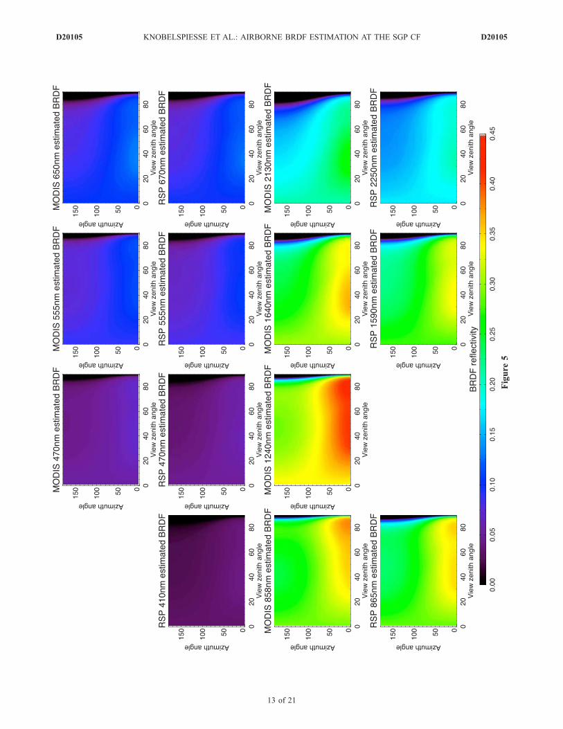
[58] The first, and most direct way of comparing BRDFestimation results from RSP and MODIS is to examine theapproximated BRDF retrievals. As described in equation(1), BRDF is a function of spectra (l), solar and viewingzenith angles (qs and qv), and the relative azimuth angle (f =fv � fs, an assumption made in most literature). Because ofthe high dimensionality, we present a ‘‘slice’’ of the BRDFestimated for the ‘‘all’’ surface class for RSP and MODIS inFigure 5. Generally speaking, the magnitude and BRDFangular dependence for RSP and MODIS are similar.Largest differences are for the longest wavelength values,where the band locations for RSP and MODIS have thegreatest dissimilarities. Better agreement in the visiblebands could also be due to their use in the classificationroutines described previously, as divergent longer wave-length reflectances are not used to identify a class.

4.2. BHR (White-Sky Albedo)

[59] Figure 6 is a plot of the spectral and broadband BHRvalues for RSP and MODIS ‘‘all’’, ‘‘soil’’ and ‘‘vegetation’’classes. Spectral dependence is very similar to the magni-tude of isotropic kernel values in Figure 5. BHR peaks areevident in the ‘‘vegetation’’ class in the green and NIRbands, while ‘‘soil’’ class BHR values are greatest at longerwavelengths. For ‘‘vegetation’’ and ‘‘soil’’ classes, RSP and

Table 3. Wang et al. [2007] Albedo Parameters

Vegetation type: Type 10: Grassland Type 12: Cropl

DHR(60�, LVIS): 0.099 0.066DHR(60�, LNIR): 0.295 0.286B1: 0.57 0.62B2: 0.12 0.13fgeo(LVIS): 0.056 0.041fvol(LVIS): 0.012 0.009fgeo(LNIR): 0.168 0.177fvol(LNIR): 0.035 0.037

Figure 5. BRDF approximation results for MODIS (first and third rows) and RSP (second and fourth rows) duringALIVE. These results are for the ‘all’ surface type class with a solar zenith angle of 30�.


12 of 21

D20105

Figure

5


13 of 21

D20105

MODIS BHR agree best in the visible wavelength bandsthat were used to classify the data, and generally agreewithin a BHR of 0.05 at other wavelengths. Broadband BHRcomparisons show similar levels of agreement, with thedifference between RSP and MODIS for the ‘‘all’’ class of0.023. The RSP ‘‘all’’ BHRbb is the closest match to theBEFLUX BHR, with a BHRbb 0.0001 greater than thatderived from BEFLUX. Interestingly, the best match ofspectral BHR between RSP and MODIS are with the ‘‘all’’classes, with similar spectral bands having differences lessthan 0.025. Although the ‘‘vegetation’’ and ‘‘soil’’ classeswere derived with the intent of creating comparable RSPand MODIS albedos, the best agreement is for the averagebehavior of the two data sets. This is presumably becausespatial averaging reduces the effects of the different spatialresolutions of the two sensors. Table 4 contains the tabu-lated BHR values displayed in Figure 6.

4.3. DHR (Black-Sky Albedo)

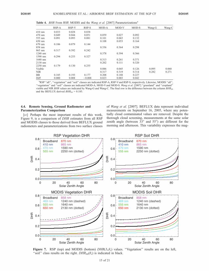
[60] Figure 7 is a plot of the DHR for each spectral bandand the broadband DHRbb. RSP vegetation and soil classesare plotted along with vegetation and soil from MODIS. Asexpected, DHRbb roughly represents the mean magnitudeand shape of the spectral DHR from which it is created. Thisis particularly true for longer wavelengths, which were moreheavily weighted in the spectral to broadband conversion

due to a combination of higher exo-atmospheric irradiance,atmospheric transmittance, and surface reflectance. Theshape and spectral variation of the DHR is similar forRSP and MODIS, as we would expect based on thesimilarity of the kernel values and the spectral BHR valuespresented in Figures 5 and 6.[61] It is important to note that estimation of the BRDF

using the kernel approach may be unphysical for anglesother than those used to estimate the BRDF. Although theDHR calculated directly from the integrals of the BRDFkernels (as given by Lucht et al. [2000b]) remains physical(positive) for the kernel values analyzed here, the underly-ing BRDF may actually have negative values for high viewor solar zenith angles. Great care should therefore beexercised in the use of these kernel estimated BRDF’s atsuch high (greater than 75�) angles.[62] Model inputs require, among other things, the shape

of DHR with respect to solar zenith angle. Yang [2006]expresses this shape by normalizing DHR by its value atqs = 60�. Figure 8 shows those normalized DHR (nDHR)values for both broadband and spectral values from the‘‘vegetation’’ and ‘‘soil’’ classes of RSP and MODIS. Here,the broadband nDHR is most similar to the longer wave-length visible or NIR nDHR. This illustrates the significanceof those bands in forming broadband DHR.

Figure 6. RSP (blue lines with diamonds) and MODIS (red lines with diamonds) BHR(L). ‘‘All’’results are on the top left, ‘‘vegetation’’ class results on the top right, and ‘‘soil’’ class results on thebottom left. Straight horizontal lines represent the broadband BHRbb, where again RSP is indicated inblue and MODIS in red. The thick black line is the BEFLUX BHRbb.


14 of 21

D20105

4.4. Remote Sensing, Ground Radiometer andParameterization Comparison

[63] Perhaps the most important results of this work,Figure 9, is a comparison of DHR estimates from all RSPand MODIS classes to those derived from BEFLUX groundradiometers and parameterizations from two surface classes

of Wang et al. [2007]. BEFLUX data represent individualmeasurements on September 16, 2005, where any poten-tially cloud contaminated values are removed. Despite thethorough cloud screening, measurements at the same solarzenith angle (between 33� and 55�) are different for themorning and afternoon. This variability expresses the mag-

Table 4. BHR From RSP, MODIS and the Wang et al. [2007] Parameterizationsa

RSP-A RSP-V RSP-S MOD-A MOD-V MOD-S Wang-G Wang-C

410 nm 0.033 0.028 0.038470 nm 0.049 0.044 0.051 0.059 0.027 0.092555 nm 0.091 0.093 0.081 0.101 0.065 0.132650 nm 0.108 0.053 0.164670 nm 0.106 0.079 0.144858 nm 0.336 0.364 0.298865 nm 0.317 0.392 0.2421240 nm 0.378 0.394 0.3661590 nm 0.294 0.253 0.3271640 nm 0.313 0.261 0.3712130 nm 0.202 0.111 0.3202250 nm 0.179 0.130 0.255Visible 0.086 0.045 0.126 0.095 0.068NIR 0.317 0.319 0.314 0.282 0.271BB 0.185 0.193 0.177 0.208 0.188 0.227Diff 0.000 0.008 �0.008 0.023 0.003 0.042

aRSP ‘‘all’’, ‘‘vegetation’’ and ‘‘soil’’ classes are indicated RSP-A, RSP-Vand RSP-S, respectively. Likewise, MODIS ‘‘all’’,‘‘vegetation’’ and ‘‘soil’’ classes are indicated MOD-A, MOD-Vand MOD-S. Wang et al. [2007] ‘‘grassland’’ and ‘‘cropland’’visible and NIR BHR values are indicated by Wang-G and Wang-C. The final row is the difference between the column BHRbb

and the BEFLUX derived BHRbb = 0.185.

Figure 7. RSP (top) and MODIS (bottom) DHR(L,qs) values. ‘‘Vegetation’’ results are on the left,‘‘soil’’ class results on the right. DHRbb(qs) is indicated in black.


15 of 21

D20105

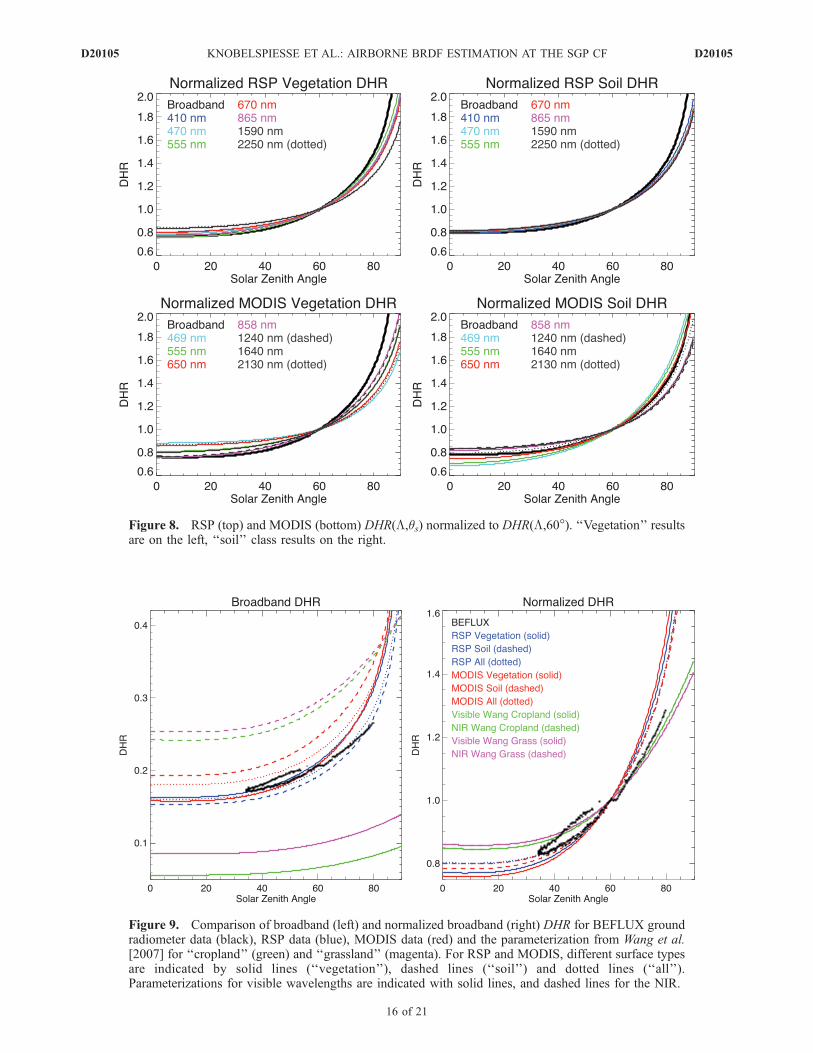
Figure 8. RSP (top) and MODIS (bottom) DHR(L,qs) normalized to DHR(L,60�). ‘‘Vegetation’’ resultsare on the left, ‘‘soil’’ class results on the right.

Figure 9. Comparison of broadband (left) and normalized broadband (right) DHR for BEFLUX groundradiometer data (black), RSP data (blue), MODIS data (red) and the parameterization from Wang et al.[2007] for ‘‘cropland’’ (green) and ‘‘grassland’’ (magenta). For RSP and MODIS, different surface typesare indicated by solid lines (‘‘vegetation’’), dashed lines (‘‘soil’’) and dotted lines (‘‘all’’).Parameterizations for visible wavelengths are indicated with solid lines, and dashed lines for the NIR.


16 of 21

D20105

nitude of potential systematic uncertainties, such as differ-ences due to solar azimuth angle or multiple ground-atmosphere interactions occurring in different areas adjacentto the radiometers.[64] While it is impossible to be sure which type of

surface class is best to compare with BEFLUX derivedDHR (as discussed in section 3.3), it is reasonable to assumethat it should be similar to one of the classes or a mixture ofthe two, as the small area of pasture where the BEFLUXradiometers are located is sampled in both RSP and MODISdata-sets. Indeed, this is the case for absolute DHR fromboth RSP and MODIS. The best matches are the RSP andMODIS ‘‘vegetation’’ classes, although other RSP classesare close as well. Of course, this comparison is limited tosolar zenith angles greater than about 33� and less thanabout 80�, as this is the range of DHR solar zenith anglesderived from BEFLUX. However, a lack of a comparisonbeyond this angular range should not be a significantproblem when evaluating kernel based estimates of DHRand BHR. As mentioned previously, very high solar zenithangles are neither routinely measured nor energeticallyimportant for climate modeling, while the data used toestimate the Ross-Li kernel values included nadir viewangles. Reciprocity of the kernel BRDF’s should thereforeensure acceptable behavior of the DHR values at small solarzenith angles. The agreement between RSP predicted andBEFLUX broadband BHR and DHR is excellent (0.0001and on average 0.0058 for BHR and DHR, respectively, inthe RSP ‘‘all’’ class) over the angular range from 30� to 80�.This indicates the capability of well corrected, multi-angle,narrowband results to predict the radiative balance at thesurface. Although we have found larger discrepancies with

MODIS results, broadband DHR agreement is still betterthan 0.0042 for even the most poorly matched surface type(‘‘soil’’).

4.5. Azimuth Angle Independence

[65] RSP estimates of the BRDF are aided by the largenumber and range of view zenith angles of measurementavailable at one time. However, the results presented hererepresent two flights (for the ‘‘vegetation’’ and ‘‘all’’classes) or one flight (for the ‘‘soil’’ class) and thereforemeasurements have a limited range of relative solar - viewazimuth angles. Thus, while BRDF estimation is based on awell sampled meridional plane the number of such planes isvery limited. While it is impossible to fully investigate theconsequences of this azimuth angle measurement limitationwithout more data, some indication of the potential vari-ability or uncertainty in BRDF estimates caused by thislimitation can be determined by comparing results from thetwo flights. Figure 10 is a comparison of BRDF estimationresults for JRF3 (relative solar - view azimuth, f = 315� forforward scans) and JRF4 (relative solar - view azimuth, f =156� for forward scans) for the ‘‘vegetation’’ class.[66] Comparisons of spectral BHR reveal inter-flight

differences equal to or less than 0.07 for angles less than80�. The maximum difference is in the 865nm band, whichfor vegetation is by far the brightest channel (see Figure 6).Broadband BHR differences are less than 0.01, less thanmost of the spectral BHR differences. It appears thatcomputation of the broadband BHR removes some of thedifference between the flights, which may be related todifferences in the observed vegetation. Spectral DHR showsa similar pattern as BHR. Maximum differences are about

Figure 10. Differences in BHR and DHR estimated from data restricted to one flight, and thus onerelative solar-view azimuth angle. The plot on the left is the difference between spectral BHR(L) andbroadband BHRbb for JRF3 and JRF4 for the ‘‘vegetation’’ class. The right side is the same forDHR(L,qs) and DHRbb(qs).


17 of 21

D20105

0.06 at 60� for the 865nm band, and increase with solarzenith angle. At solar zenith angles less than 80�, the flightto flight DHRbb difference is about 0.01.

5. Discussion

[67] The foremost purpose of this paper is to evaluateMODIS BRDF estimates. This is done by comparingMODIS derived BHR and DHR (white and black skyalbedos, in MODIS terminology) to the same values derivedfrom an airborne sensor (RSP) and a group of groundradiometers (BEFLUX) during September in north-centralOklahoma. This is a region whose ground cover mainlyincluded grassland and late season or recently harvestedcropland. This location is important because of the presenceof the SGP CF, where a host of atmospheric and radiometricinstruments provide a continuous set of validation data.MODIS overestimates BHRbb with respect to BEFLUX bybetween 0.003 and 0.042 (depending on the surface class,see Table 4). The average MODIS DHR deviation (over allangles less than 80�) from BEFLUX is 0.018, �0.002 and0.035 for the ‘‘all’’, ‘‘vegetation’’ and ‘‘soil’’ classes, respec-tively. Considering that BEFLUX derived DHR has differ-ences up to 0.01 between measurements with the samesolar zenith angle but at different times of day (morningand evening), we regard the MODIS DHR estimates assuccessful.[68] An important component of any validation work is to

identify which differences are due to the data processingnecessary to perform the validation, and which representactual instrumental differences. In this case, we recognizeseveral processing steps that may add to or mask actualinstrumental differences. Both RSP and MODIS were fit toRoss-Li BRDF models, and thus are only capable ofmeasuring the types of BRDF that are included in thosemodels. Another potential source of error is the need tocreate broadband BHR and DHR from spectral RSP andMODIS values, in order to compare to naturally broadbandBEFLUX derived values. This involves interpolating be-tween spectral bands prior to integration to broadbandvalues, and this interpolation could miss spectral variationin the BHR or DHR that is included in the broadband valuesderived from BEFLUX. Finally, spatial and temporal reso-lution differences between satellites and point sensors on theground are a well known source of error. We have attemptedto account for these problems by separating the data intocomparable classes roughly representing vegetated crops orgrassland and bare (recently harvested) soil. MODIS andRSP classes are consistent with one another (see Figures 6,7, 8 and 9), and closest with the ‘‘all’’ classes containing theentire dataset prior to classification. As Figure 4 shows,RSP and MODIS data-sets have a somewhat differentspatial extent. So, while the classification techniques forRSP and MODIS may not be compatible, other aspects ofRSP and MODIS data processing (such as spectral tobroadband conversion and model fitting) produce remark-ably similar results. MODIS BHRbb shows a bias withrespect to RSP of 0.023, �0.005 and 0.050 for the ‘‘all’’,‘‘vegetation’’ and ‘‘soil’’ classes, respectively. Average(with respect to solar zenith angles less than 80�) biasesfor DHRbb between MODIS and RSP are 0.036, 0.006 and

0.076 for the ‘‘all’’, ‘‘vegetation’’ and ‘‘soil’’ classes,respectively. nDHRbb has an average bias typically anorder of magnitude less than absolute DHRbb, indicatingthat differences between the instruments are primarily dueto differences in the absolute magnitude of their estimates.MODIS-RSP comparisons of individual spectral bandsshow the same small bias for both DHR and nDHR.[69] This research began as an effort to investigate some

of the differences between BEFLUX radiometers andMODIS parameterizations identified by Yang [2006]. Weimplemented the novel DHR BEFLUX computation tech-nique described in that paper, but did so for the much morelimited time range of the ALIVE campaign. Yang [2006]compared nDHR to parameterizations described by Wang etal. [2007] and Liang et al. [2005], and found the BEFLUXderived values to be larger than both parameterizations atsolar zenith angles greater than 80�, and more troubling,smaller than parameterizations at angles less than 35�.Yang’s comparison utilized a third order polynomial fitbecause its similarity to an approximation given in Schaafet al. [2002]. However, unlike the standard third-orderpolynomial that Yang used, the polynomial in Schaaf etal. [2002] is restricted to have a zero coefficient on the first-order term. Figure 11 presents the difference between thesetwo fitting routines, where we fit both types of polynomialsto our BEFLUX data. Schaaf’s polynomial fit clearlymatches RSP and MODIS DHR and nDHR, while the Yangpolynomial diverges in a similar manner to that presented inYang [2006]. Thus, the biases that were identified in Yang[2006] are both beyond the solar zenith angle range of thereference dataset and most likely due to the choice of thedata fit, rather than the data itself.[70] The albedo parameterization presented in Wang et al.

[2007] is also included in the comparison in Figure 9.Wang’s parameterization, described in section 3.4, is anattempt to reduce the number of parameters describingMODIS albedo from three for each band to two each forbroad visible and NIR bands (which are specified forvarious surface types). Although these broad visible andNIR channels cannot be compared directly to broadbandBEFLUX DHR, the Wang et al. [2007] nDHR is spectrallyinvariant, and thus can be compared to BEFLUX derivednDHR. Figure 9 shows that both of the selected surfaces(grass and cropland) produce nDHR with slightly shallowerslopes than BEFLUX derived nDHR. Thus, Wang’s param-eterizations show slightly smaller variation in DHR as afunction of solar zenith angle compared to BEFLUX.Average (for solar zenith angle less than 80�) biases fornDHR are between 0.022 and 0.028, depending on the landsurface type selected for the parameterization.

6. Conclusion

[71] Generally speaking, this validation shows that thereis good agreement between MODIS, RSP and BEFLUXground radiometer derived albedos, at least for the con-ditions of the ALIVE experiment at the SGP CF. MODIS,which is capable of producing global BRDF estimates,produces DHR and BHR (‘‘black-sky’’ and ‘‘white-sky’’,albedos, respectively) that agree with aircraft measurementsfrom RSP. RSP has a higher spatial and temporal resolution


18 of 21

D20105

than MODIS, and its data are atmospherically correctedwith more sophisticated algorithms, yet differences betweenthe two are minimal. It is important to note that RSP usedthe same Ross-Li BRDF models employed by MODIS, sosome potential instrumental differences may be masked bythis similarity. However, model fitting results are robust andphysically realistic. RSP and MODIS also agree well withDHR and BHR derived from the BEFLUX ground radio-meters, whose methodology is quite different than theBRDF model fitting routines employed by the remotesensing instruments. A potential source of non-instrumentalcomparison error are the methods used to convert spectralDHR and BHR to broadband values. In our case we wererequired to interpolate spectral albedos and model theground-atmosphere interaction. Previously identified differ-ences between BEFLUX ground radiometers and MODISwere shown to be for DHR in solar zenith angles beyond therange of available comparison angles and were most likelydue to the choice of the type of polynomial fit to the data,rather than instrumental effects in the data itself.[72] This validation effort is hindered by the small quan-

tity of data available for comparison. Cloud free, lowaltitude RSP measurements were limited to a single day(September 16, 2005) during the ALIVE campaign. RSPserves as an airborne prototype to the Aerosol PolarimeterySensor (APS), due to be launched as part of the NASAGlory mission in 2008. APS is not an imaging instrumentand will not be able to create global BRDF estimates likeMODIS. However, the rapid angular scanning and accurateatmospheric correction of APS means that it is an idealplatform for validation of BRDF estimates from MODISand other instruments. Pending a successful launch, Glorywill join the NASA ‘A-train’ orbit, and APS will begingathering a validation dataset much larger than what was

available for the work in this paper. The methods used herecould become part of a routine BRDF remote sensingvalidation effort.

Appendix A: Correction for Gas Absorption

[73] Prior to assessing ground reflectance, water vapor,ozone and NO2 absorption effects were removed from thedirect solar beam. Water vapor was measured at SGP CFwith a MWR, while ozone and NO2 measurements wereprovided by the TOMS and SCIAMACHY orbital instru-ments, respectively. Absorption coefficients were computedusing the spectral sensitivity of each RSP band, and appliedto RSP measurements as follows:

Ic ¼ I e�M KO3xO3þKNO2

xNO2ð Þ�a wM½ �bÞ� ��1

ðA1Þ

where I and Ic are the original and corrected radiances,respectively. KO3

is the ozone absorption coefficient, xO3 isthe ozone quantity in centimeters per atmosphere, KNO2

isthe NO2 absorption coefficient, xNO2

is the quantity of NO2

in parts per billion, w is the column water vapor, incentimeters, and parameters a and b define the opticaldepth due to water vapor. a, b, Koz and KNO2

are given inTable A1. M is the airmass, which defines the length of theatmospheric path from the sun to the Earth surface and iswell approximated for the solar zenith angles encounteredhere by M = cos(qs)

�1. The use of the correction proceduredefined by equation (A1) is justified for ozone and nitrogendioxide by the fact that they absorb light primarily in thestratosphere, above most atmospheric scattering. It isacceptable for water vapor because this only affects RSPbands at 1590 and 2250 nm, for which single scattering is avalid approximation of the effects of aerosols and

Figure 11. BEFLUX derived DHR (left) and nDHR (right) and the corresponding polynomial fits to oursubset of BEFLUX data, as described by Yang [2006] (green) and Schaaf et al. [2002] (blue). OriginalBEFLUX derived DHR are in black. For comparison, the ‘‘all’’ classes of RSP (magenta) and MODIS(red) are also included.


19 of 21

D20105

molecules. Gas quantities for the day of our experimentwere: 0.285 Dobson Units of Ozone, 0.74 ppb of NO2, andprecipitable water vapor between 1.237 and 1.498 cm,depending on the time of day.

Appendix B: Vegetation Indicies

[74] The canonical method for assessing surface vegeta-tion content is the Normalized Difference Vegetation Index(NDVI):

NDVI ¼ LNIR � Lred

LNIR þ LredðB1Þ

where L is the radiance detected by a red or near-infra red(NIR) sensor. Vegetation has a low reflectance at redwavelengths, and much higher reflectance in the NIR, whilesoils and other non-vegetated surfaces have much smallerspectral contrast between the red and NIR. NDVI has beenused for years to assess vegetation health and cover fromspace, although it is important to note that it is simply anindex not an actual physical parameter. However, there isthe possibility that the spectral dependence of the aerosoloptical properties modifies LNIR and Lred in a manner thataffects NDVI [Kaufman and Tanre, 1992]. We thereforeused Kaufman and Tanre’s Atmospherically ResistantVegetation Index (ARVI) which is less sensitive to theeffects of atmospheric aerosols [Kaufman and Tanre, 1992].ARVI uses a channel at a blue wavelength in order tocorrect for atmospheric effects. It is defined in terms ofnormalized reflectances as:

ARVI ¼ rNIR � rrbrNIR þ rrb

rrb ¼ rred � g rblue � rredð Þ ðB2Þ

where g is a parameter that depends on the aerosol type. Weused a value of g = 0.9 as suggested by Kaufman and Tanrefor continental aerosols. RSP channels 2 (470 nm), 4 (670 nm)and 5 (865 nm) were used for rblue, rred, and rNIR,respectively.

[75] Acknowledgments. The first author acknowledges support fromthe US National Science Foundation, through a Fellowship in the IGERTJoint Program in Applied Mathematics and Earth and EnvironmentalScience at Columbia University at the time of the ALIVE field campaign.BEFLUX data were obtained from the Atmospheric Radiation Measure-ment (ARM) Program sponsored by the U.S. Department of Energy, Officeof Science, Office of Biological and Environmental Research, Environ-mental Sciences Division. ALIVE was also funded by ARM, and RSPparticipation during that experiment was funded by the National Aeronau-tics and Space Administration (NASA). Thanks to the many who helpedcollect the data used in this study: Ben Hovelman was the J-31 pilot, RoyJohnson and Nicholas Truong were AATS-14 engineers, Rose Dominguez

provided J-31 Navigational and GPS data, and Warren Gore provided J-31Meteorological data. Finally, thanks to both the anonymous reviewers.

ReferencesBovensmann, H., J. Burrows, M. Buchwitz, J. Frerick, S. Noel, V. Rozanov,K. Chance, and A. Goede (1999), SCIAMACHY: Mission Objectivesand Measurement Modes, J. Atmos. Sci., 56(2), 127–150.

Bruegge, C., M. Helmlinger, J. Conel, B. Gaitley, and W. Abdou (2000),PARABOLA III- A sphere-scanning radiometer for field determination ofsurface anisotropic reflectance functions, Remote Sens. Rev., 19(1), 75–94.

Cairns, B. (2003), Polarimetric remote sensing of aerosols, IEEE Trans.Geosci. Remote Sens., 518–520.

Cairns, B., B. Carlson, R. Ying, A. Lacis, and V. Oinas (2003), Atmo-spheric correction and its application to an analysis of Hyperion data,IEEE Trans. Geosci. Remote Sens., 41(6), 1232–1245.

Chahine, M. (1968), Determination of the temperature profile in an atmo-sphere from its outgoing radiance, J. Opt. Soc. Am, 58, 1634–1637.

Chowdhary, J., B. Cairns, and L. Travis (2002), Case studies of aerosolretrievals over the ocean from multiangle, multispectral photopolarimetricremote sensing data, J. Atmos. Sci., 59(3), 383–397.

de Haan, J., P. Bosma, and J. Hovenier (1987), The adding method formultiple scattering calculations of polarized light, Astron. Astrophys.,183(2), 371–391.

Dubovik, O., andM. King (2000), A flexible inversion algorithm for retrievalof aerosol optical properties from sun and sky radiance measurements,J. Geophys. Res., 105(D16), 20,673–20,696.

Engelsen, O., B. Pinty, M. Verstraete, and J. Martonchik (1998), Parametricsurface bidirectional reflectance factor models for atmospheric radiativetransfer modeling, Geoscience and Remote Sensing Symposium Proceed-ings (1998), IGARSS’98. 1998 IEEE International, 2, 713–715.

Gatebe, C., M. King, S. Platnick, G. Arnold, E. Vermote, and B. Schmid(2003), Airborne spectral measurements of surface-atmosphere anisotro-py for several surfaces and ecosystems over southern Africa, J. Geophys.Res., 108(D13), 8489, doi:10.1029/2002JD002397.

Gonzalez, R., and R. Woods (1992), Digital Image Processing, AddisonWesley Publishing Company, New York.

Hansen, J., and L. Travis (1974), Light scattering in planetary atmospheres,Space Sci. Rev., 16, 527–610.

Holben, B., Y. Kaufman, T. Eck, I. Slutsker, D. Tanre, J. Buis, A. Setzer,E. Vermote, and J. Reagan (1998), Aeronet-a federated instrument networkand data archive for aerosol characterization, Remote Sens. Environ., 66,1–16.

Hovenier, J. (1971), Multiple Scattering of Polarized Light in PlanetaryAtmospheres, Astron. Astrophys., 13, 7.

Jin, Y., C. Schaaf, C. Woodcock, F. Gao, X. Li, A. Strahler, W. Lucht, andS. Liang (2003), Consistency of modis surface bidirectional reflectancedistribution function and albedo retrievals: 2. Validation, J. Geophys.Res., 108(D5), 4159, doi:10.1029/2002JD002804.

Kaufman, Y. J., and D. Tanre (1992), Atmospherically resistant vegetationindex (arvi) for eos-modis, IEEE Trans. Geosci. Remote Sens., 30, 261–270.

Lacis, A., and J. Hansen (1974), A parameterization for the absorption ofsolar radiation in the earth’s atmosphere, J. Atmos. Sci., 31(1), 118–133.

Li, X., and A. Strahler (1992), Geometric-optical bidirectional reflectancemodeling of thediscrete crown vegetation canopy: Effect of crown shapeand mutualshadowing, IEEE Trans. Geosci. Remote Sens., 30(2), 276–292.

Liang, S. (2001), Narrowband to broadband conversions of land surfacealbedo. I: Algorithms, Remote Sens. Environ., 76(2), 213–238.

Liang, S., H. Fang,M. Chen, C. Shuey, C.Walthall, C. Daughtry, J.Morisette,C. Schaaf, and A. Strahler (2002), Validating MODIS land surfacereflectance and albedo products—Methods and preliminary results, Re-mote Sens. Environ., 83(1), 149–162.

Liang, S., C. Shuey, A. Russ, H. Fang, M. Chen, C. Walthall, C. Daughtry,and R. Hunt Jr. (2003), Narrowband to broadband conversions of landsurface albedo. II: Validation, Remote Sens. Environ., 84(1), 25–41.

Liang, X.-Z., et al. (2005), Development of land surface albedo parameter-ization based on moderate resolution imaging spectroradiometer (modis)data, J. Geophys. Res., 110, D11107, doi:10.1029/2004JD005579.

Long, C., D. Slater, and T. Tooman (2001), Total Sky Imager Model 880Status and Testing Results, Pacific Northwest National Laboratory, Atmo-spheric Radiation Measurement Program, Richland, WA.

Lucht, W., A. Hyman, A. Strahler, M. Barnsley, P. Hobson, and J. Muller(2000a), A comparison of satellite-derived spectral albedos to ground-based broadband albedo measurements modeled to satellite spatial scalefor a semidesert landscape, Remote Sens. Environ., 74(1), 85–98.

Lucht, W., C. Schaaf, and A. Strahler (2000b), An algorithm for the retrie-val of albedo from space using semiempirical brdf models, IEEE Trans.Geosci. Remote Sens., 38(2), 977–998.

Table A1. Gas Absorption Parameters

Band Wavelength KO3KNO2

a b

1 410 0.000278 0.012860 0.00000 1.0000002 469 0.010035 0.008135 0.00000 1.0000003 555 0.096960 0.001827 0.00026 0.9900684 670 0.044982 0.000144 0.00053 0.9587425 864 0.002060 0.000000 0.00061 0.9537747 1589 0.000000 0.000000 0.00251 0.6453479 2264 0.000000 0.000000 0.01141 0.739948


20 of 21

D20105

Luo,Y., A. Trishchenko, R. Latifovic, and Z. Li (2003), Surface bi-directionalreflectance properties over the arm sgp area from satellite multi-platformobservations, in Proceedings of the Thirteenth Atmospheric RadiationMeasurement (ARM) Science Team Meeting, edited by D. Carrothers,pp. 1–12, Department of Energy, Richland, Wash.

Luo, Y., A. P. Trishchenko, R. Latifovic, and Z. Li (2005), Surface bidirec-tional reflectance and albedo properties derived using a land cover basedapproach with moderate resolution imaging spectroradiometer observa-tions, J. Geophys. Res., 110, D01106, doi:10.1029/2004JD004741.

Martonchik, J., D. Diner, K. Crean, and M. Bull (2002), Regional aerosolretrieval results from misr, IEEE Trans. Geosci. Remote Sens., 40(7),1520–1532.

McPeters, R., and G. Center (1998), Earth Probe Total Ozone MappingSpectrometer (TOMS) Data Product User’s Guide, NASA TP-1998-206895, National Aeronautics and Space Administration, Goddard SpaceFlight Center; National Technical Information Service.

Mishchenko, M., B. Cairns, J. Hansen, L. Travis, R. Burg, Y. Kaufman,J. Vanderlei Martins, and E. Shettle (2004), Monitoring of aerosol forcingof climate from space: Analysis of measurement requirements, J. Quant.Spectrosc. Radiat. Transfer, 88(1–3), 149–161.

Mishchenko, M., I. Geogdzhayev, B. Cairns, B. Carlson, J. Chowdhary,A. Lacis, L. Liu, W. Rossow, and L. Travis (2007a), Past, present, andfuture of global aerosol climatologies derived from satellite observations:A perspective, J. Quant. Spectrosc. Radiat. Transfer, 106, 325–347.

Mishchenko, M., B. Cairns, G. Kopp, C. F. Schueler, B. A. Fafaul, J. E.Hansen, R. J. Hooker, T. Itchkawich, H. B. Maring, and L. D. Travis(2007b), Accurate monitoring of terrestrial aerosols and total solar irra-diance: Introducing the Glory mission, Bull. Amer. Meteorol., 88.

Morris, V. (2006), Microwave radiometer (mwr) handbook, Tech. Rep.ARM TR-016, U.S. Department of Energy, Argonne, IL.

Myhre, G., and A. Myhre (2003), Uncertainties in radiative forcing due tosurface albedo changes caused by land-use changes, J. Clim., 16(10),1511–1524.

Nicodemus, F. E., J. C. Richmond, J. J. Hsia, I. W. Ginsberg, and T.Limperis (1977), Geometrical Considerations and Nomenclature for Re-flectance, US Dept. of Commerce, National Bureau of Standards, Supt. ofDocs., US Govt. Print. Off., Washington, D. C.

Pinty, B., A. Lattanzio, J.Martonchik,M. Verstraete, N. Gobron,M. Taberner,J. Widlowski, R. Dickinson, and Y. Govaerts (2005), Coupling DiffuseSky Radiation and Surface Albedo, J. Atmos. Sci., 62(7), 2580–2591.

Ross, J. (1981), The Radiation Regime and Architecture of Plant Stands,W. Junk, Norwell, Mass.

Roujean, J., M. Leroy, and P. Deschanps (1992), A bidirectional reflectancemodel of the Earth’s surface for the correction of remote sensing data,J. Geophys. Res., 97(D18), 20,455–20,468.

Salomon, J., C. Schaaf, A. Strahler, F. Gao, and Y. Jin (2006), Validation ofthe MODIS bidirectional reflectance distribution function and albedo

retrievals using combined observations from the aqua and terra platforms,IEEE Trans. Geosci. Remote Sens., 44(6), 1555–1565.

Schaaf, C., A. Strahler, M. Roman, J. Salomon, and J. Hodges (2006),Assessment of albedo derived from the moderate-resolution imagingspectroradiometer at the southern great plains site, in Proceedings ofthe Sixteenth ARM Science Team Meeting, pp. 1–2, Department of En-ergy Atmospheric Radiation Measurement Program, Albuquerque, NM.

Schaaf, C., F. Gao, A. H. Strahler, W. Lucht, X. Li, T. Tsang, N. C.Strugnell, X. Zhang, Y. Jin, and J. P. Muller (2002), First operationalBRDF, albedo nadir reflectance products from MODIS, Remote Sens.Environ., 83(1), 135–148.

Schaepman-Strub,G.,M. Schaepman, T. Painter, S.Dangel, and J.Martonchik(2006), Reflectance quantities in optical remote sensing: Definitions andcase studies, Remote Sens. Environ., 103(1), 27–42.

Schmid, B., et al. (2006), How well do state-of-the-art techniques measur-ing the vertical profile of tropospheric aerosol extinction compare,J. Geophys. Res., 111, D05507, doi:10.1029/2005JD005837.

Shi, Y., and C. Long (2002), Best Estimate Radiation Flux Value-added Pro-cedure: Algorithm Operational Details and Explanations, ARM TR-008,Pacific Northwest National Laboratory, Richland, WA.

Strahler, A., W. Lucht, C. Schaaf, T. Tsang, F. Gao, X. Li, J. Muller, P. Lewis,and M. Barnsley (1999), MODIS BRDF/Albedo Product: Algorithm The-oretical Basis Document Version 5.0, Tech. rep., National Aeronautics andSpace Administration.

Twomey, S. (1977), The Influence of Pollution on the Shortwave Albedo ofClouds, J. Atmos. Sci., 34(7), 1149–1152.

Wang, Z., X. Zeng, and M. Barlage (2007), Moderate resolution imagingspectroradiometer bidirectional reflectance distribution function-basedalbedo parameterization for weather and climate models, J. Geophys.Res., 112, D02103, doi:10.1029/2005JD006736.

Wanner, W., X. Li, and A. Strahler (1995), On the derivation of kernel-driven models of bidirectional reflectance, J. Geophys. Res., 100(D10),21,077–21,090.

Yang, F. (2006), Parameterizing the dependence of surface albedo on solarzenith angle using atmospheric radiation measurement observations, inProceedings of the Sixteenth ARM Science Team Meeting Proceedings,Alburquerque, NM.

��B. Cairns and K. D. Knobelspiesse, Department of Applied Physics and

Applied Mathematics, Columbia University, NASA GISS, 2880 Broadway,New York, NY 10025, USA. ([email protected])M. O. Roman and C. B. Schaaf, Department of Geography and

Environment, Center for Remote Sensing, Boston University, 675Commonwealth Avenue STO-457, Boston, MA 02215, USA.B. Schmid, Atmospheric Science and Global Change Division, Pacific

Northwest National Laboratory, 902 Battelle Boulevard, P.O. Box 999,MSIN K9-24, Richland, WA 99352, USA.


21 of 21

D20105

Surface BRDF estimation from an aircraft compared to MODIS and ...

Documents

Transcript of Surface BRDF estimation from an aircraft compared to MODIS and ...