Modeling the non-linear dynamics of calcium in chromaffin … · Resumo Em resposta ao medo ou...
76
Modeling the non-linear dynamics of calcium in chromaffin cells Inˆ es Filipa Completo Guerreiro Thesis to obtain the Master of Science Degree in Engineering Physics Supervisors: Prof. Maria Teresa Ferreira Marques Pinheiro Prof. David Gall Examinatiom Committee Chairperson: Prof. Lu´ ıs Filipe Moreira Mendes Supervisor: Prof. Maria Teresa Ferreira Marques Pinheiro Member of the Committe: Prof. Hugo Fernando Santos Terc ¸as September 2015
Transcript of Modeling the non-linear dynamics of calcium in chromaffin … · Resumo Em resposta ao medo ou...

Modeling the non-linear dynamics of calcium inchromaffin cells
Ines Filipa Completo Guerreiro
Thesis to obtain the Master of Science Degree in
Engineering Physics
Supervisors: Prof. Maria Teresa Ferreira Marques PinheiroProf. David Gall
Examinatiom CommitteeChairperson: Prof. Luıs Filipe Moreira Mendes
Supervisor: Prof. Maria Teresa Ferreira Marques PinheiroMember of the Committe: Prof. Hugo Fernando Santos Tercas
September 2015


Acknowledgments
I would like to thank my supervisors, Prof. Maria Teresa Pinheiro from Instituto Superior Tecnico
and Prof. David Gall from the Universite Libre de Bruxelles, for all the patience and availability to
answer all my questions, and for their guidance throughout all the work. I also want to thank Prof.
Genevieve Dupont from the Universite Libre de Bruxelles, who was a precious help in the development
of this work.
Finally, I would like to thank my family and close friends for all the support, not only during the time
I worked on this project, but throughout the entire course.
i


Resumo
Em resposta ao medo ou stress, celulas cromafins (celulas encontradas principalmente na medula
das glandulas supra-renais, localizadas acima dos rins) secregam catecolaminas como a adrenalina
na nossa corrente sanguınea. A secrecao e controlada por oscilacoes de calcio intracelular, que
podem ser medidas experimentalmente.
Medicoes experimentais de calcio em celulas de cromafina de ratos demonstram que diferentes
celulas pertencentes a uma mesma populacao, quando submetidas a um mesmo estımulo, apresen-
tam diferentes padroes oscilatorios. A origem desta heterogeneidade nos padroes oscilatorios e uma
questao em aberto.
Esta tese apresenta um novo modelo matematico que descreve a dinamica nao-linear do calcio
em celulas cromafins, onde oscilacoes de calcio sao produzidas pela interacao entre a atividade
eletrica da membrana celular e a libertacao de calcio do retıculo endoplasmatico. Este novo modelo
foi construıdo juntando e adaptando dois modelos existentes: o modelo de Gall-Susa, que descreve
as oscilacoes de calcio intracelular em celulas pancreaticas tendo em conta a atividade eletrica da
celula, e o modelo de Li-Rinzel, que descreve as oscilacoes de calcio tendo em conta o fluxo de
calcio vindo a partir do retıculo endoplasmatico para o citosol atraves dos receptores IP3 presentes
na sua membrana. A validade do nosso modelo foi estudada reproduzindo algumas observacoes ex-
perimentais. Nomeadamente, estudou-se o comportamento do modelo na presenca de agentes far-
macologicos a que as celulas foram submetidas experimentalmente. Para alem disso, reproduziram-
se ambos os padroes oscilatorios observados experimentalmente, apresentando-se uma explicacao
plausıvel e razoavel para a existencia dos mesmos: os dois diferentes padroes oscilatorios observa-
dos resultam da existencia de celulas de diferentes tamanhos na populacao analisada.
Palavras-Chave
Celulas cromafins, oscilacoes de calcio intra-celular, receptor IP3, dinamica nao-linear
iii

Abstract
In response to fear or stress, chromaffin cells (cells found mostly in the medulla of the adrenal
glands, located above the kidneys) secrete catecholamines like adrenaline into our bloodstream. Se-
cretion is controlled by intracellular calcium concentration oscillations, which can be measured exper-
imentally.
Experimental measurements of calcium in rat chromaffin cells show that different cells from the
same population display different oscillatory patterns. The origin of this heterogeneity remains an
open question.
In this thesis we construct a new mathematical model that describes the non-linear dynamics of
intracellular calcium in chromaffin cells where calcium oscillations are produced by the interplay be-
tween the electrical activity of the cell membrane and the release of calcium from the endoplasmic
reticulum. We do that by coupling and adapting two existing models: Gall-Susa model, which de-
scribes intracellular calcium oscillations in pancreatic β-cells having into account the electrical activity
of the cell and Li-Rinzel model, which describes calcium oscillations having into account a flux cal-
cium coming from the endoplasmic reticulum into the cytosol through IP3 receptors present in its
membrane. We study the validity of our model by reproducing experimental observations. Namely,
we study the behavior of the model in the presence of pharmacological agents and we reproduce
both oscillatory patterns observed.
We find that a difference in the radius of the cells where the intracellular calcium concentrations
were measured provides a reasonable testable explanation for the existence of different types of
oscillations observed in chromaffin cells.
Keywords
Chromaffin cells, intracellular calcium oscillations, IP3 receptor, non-linear dynamics
iv

Contents
1 Introduction 3
1.1 Intracellular Calcium Dynamics . . . . . . . . . . . . . . . . . . . . . . . . . . . . . . . . 4
1.1.1 Calcium oscillations in chromaffin cells . . . . . . . . . . . . . . . . . . . . . . . . 4
1.1.2 Regulation of intracellular calcium . . . . . . . . . . . . . . . . . . . . . . . . . . 6
1.1.3 Models for calcium oscillations . . . . . . . . . . . . . . . . . . . . . . . . . . . . 7
1.2 Electrical Properties of the Cell Membrane . . . . . . . . . . . . . . . . . . . . . . . . . 10
1.2.1 Chromaffin cells are excitable cells . . . . . . . . . . . . . . . . . . . . . . . . . . 11
1.2.2 The origin of membrane potential . . . . . . . . . . . . . . . . . . . . . . . . . . . 11
1.2.2.A Ion channels and transporters . . . . . . . . . . . . . . . . . . . . . . . 13
1.2.3 Equivalent circuit of the cell membrane . . . . . . . . . . . . . . . . . . . . . . . 15
1.2.4 Models for membrane potential oscillations . . . . . . . . . . . . . . . . . . . . . 17
1.3 Aim of the Work . . . . . . . . . . . . . . . . . . . . . . . . . . . . . . . . . . . . . . . . 20
2 Dynamics of theoretical models 23
2.1 Li-Rinzel model . . . . . . . . . . . . . . . . . . . . . . . . . . . . . . . . . . . . . . . . . 24
2.2 Gall-Susa model . . . . . . . . . . . . . . . . . . . . . . . . . . . . . . . . . . . . . . . . 27
3 A new model for Ca2+ oscillations in chromaffin cells 35
3.1 New model . . . . . . . . . . . . . . . . . . . . . . . . . . . . . . . . . . . . . . . . . . . 36
3.2 Study of the behavior of the model in the presence of pharmacological agents . . . . . . 45
3.3 Influence of the cell capacitance on the Ca2+ oscillatory patterns . . . . . . . . . . . . . 47
4 Conclusions and Perspectives 49
Bibliography 53
Appendix A Appendix A A-1
A.1 XPPAUT . . . . . . . . . . . . . . . . . . . . . . . . . . . . . . . . . . . . . . . . . . . . . A-2
A.2 Equations and Parameters . . . . . . . . . . . . . . . . . . . . . . . . . . . . . . . . . . A-2
A.3 *.ode Files . . . . . . . . . . . . . . . . . . . . . . . . . . . . . . . . . . . . . . . . . . . . A-4
v


List of Figures
1.1 Experimental measurements of calcium in rat chromaffin cells provided by Dr. A. Mar-
tinez, Faculty of Medicine of Universidad Autonoma de Madrid . . . . . . . . . . . . . . 5
1.2 Schematic representation of the one-pool model for signal-induced calcium oscillations. 7
1.3 Schematic representation of the channel gating kinetics of the De Young-Keizer model
with the possible states of a subunit . . . . . . . . . . . . . . . . . . . . . . . . . . . . . 8
1.4 Steady state open probability of the IP3 receptor as a function of cytosolic calcium
concentration from the De Young-Keizer model. . . . . . . . . . . . . . . . . . . . . . . . 9
1.5 Schematic view of the cell membrane and the different mechanisms of ionic transport. . 12
1.6 Permeable selectivity of the cell membrane. . . . . . . . . . . . . . . . . . . . . . . . . . 12
1.7 A single-channel recording using the patch-clamp technique . . . . . . . . . . . . . . . . 14
1.8 Measurement of channel currents in response to different voltage pulses . . . . . . . . . 14
1.9 Comparison of the cell membrane and its equivalent electrical circuit. . . . . . . . . . . 15
1.10 Overall current produced by an ionic specie. . . . . . . . . . . . . . . . . . . . . . . . . . 16
1.11 Equivalent electrical circuit of the cell membrane (Hodgkin and Huxley, 1952) . . . . . . 17
2.1 Reproduction of the time course of the intracellular calcium concentrations and of the
variable p for the Li-Rinzel model. . . . . . . . . . . . . . . . . . . . . . . . . . . . . . . . 25
2.2 Bifurcation diagram of the Li-Rinzel model as a function of the inositol 1,4,5-trisphosphate
concentration . . . . . . . . . . . . . . . . . . . . . . . . . . . . . . . . . . . . . . . . . . 26
2.3 Reproduction of the time courses of the electrical activity, V, the gating variable, n, and
calcium concentrations in the cytosol and in the ER for the Gall and Susa model. . . . . 29
2.4 Overlap of the graphs for the membrane potential and the calcium concentration in the
ER . . . . . . . . . . . . . . . . . . . . . . . . . . . . . . . . . . . . . . . . . . . . . . . . 30
2.5 Time course of V for the reduced 2-variable fast subsystem of Gall-Susa model. . . . . 31
2.6 Bifurcation diagram of the reduced 2-variable fast subsystem of Gall-Susa model . . . 31
2.7 Sketch of the bifurcation diagram of the Gall-Susa model . . . . . . . . . . . . . . . . . 32
3.1 Experimental observations where the electrical activity of cell membrane is measured
in parallel with the variation of cytosolic calcium . . . . . . . . . . . . . . . . . . . . . . . 36
3.2 Scheme of fluxes and currents in the cell. . . . . . . . . . . . . . . . . . . . . . . . . . . 37
3.3 Reproduction of the time courses of all the variables of the final model. . . . . . . . . . . 40
3.4 Comparison of predict results with experimental results . . . . . . . . . . . . . . . . . . 41
vii

3.5 Time course of V for the reduced 3-variable fast subsystem of the new model. . . . . . . 42
3.6 Bifurcation diagram of the reduced 3-variable fast subsystem of the new model . . . . . 42
3.7 Sketch of the bifurcation diagram of the final model with calcium concentration in the
ER as a bifurcation parameter. . . . . . . . . . . . . . . . . . . . . . . . . . . . . . . . . 43
3.8 Overlap of the graphs for the membrane potential and the calcium concentration in the
ER for the new model. . . . . . . . . . . . . . . . . . . . . . . . . . . . . . . . . . . . . . 44
3.9 Bifurcation diagram of final model with v1 as a bifurcation parameter . . . . . . . . . . . 45
3.10 Comparison of the predict results with experimental results when the IP3 channels are
inhibited . . . . . . . . . . . . . . . . . . . . . . . . . . . . . . . . . . . . . . . . . . . . . 46
3.11 Time course of the intracellular calcium concentrations for the new model with C = 4800
fF . . . . . . . . . . . . . . . . . . . . . . . . . . . . . . . . . . . . . . . . . . . . . . . . 47
3.12 Time courses the intracellular calcium concentrations for the final model for two different
sets of parameters. . . . . . . . . . . . . . . . . . . . . . . . . . . . . . . . . . . . . . . . 48
viii

List of Tables
A.1 Parameter Values of final model . . . . . . . . . . . . . . . . . . . . . . . . . . . . . . . A-3
ix

Abbreviations
IP3: inositol (1,4,5)-trisphosphate
ER: Endoplasmic reticulum
ATP : Adenosine triphosphate
CICR: Calcium-induced calcium release
LV A: Low voltage activated
HV A: High voltage activated
HB: Hopf bifurcation
APB: Aminoethoxydiphenye bonate
1


1Introduction
Calcium concentration oscillations in chromaffin cells were measured and it was observed that
cells from a same population, submitted to the same external stimulus, present two distinct patterns
of calcium oscillations. It is not known why this happens and, until the moment, none of the existing
models that describes calcium oscillations in chromaffin cells is able to reproduce both patterns ob-
served experimentally. Given that calcium oscillations control the secretion of adrenaline and other
substances into our bloodstream [1] and, consequently, the functional response of our body to danger,
different patterns of calcium oscillations are most likely going to result in different functional responses.
The work is divided into four chapters. In this first chapter we explain how the intracellular calcium
concentration is regulated in chromaffin cells. Namely, we study how IP3 receptors present in the
membrane of the endoplasmic reticulum (ER) and the electrical activity of the cell membrane control
the intracellular calcium concentrations. We also introduce the mechanisms underlying the models
that will be used in the construction of our new model, the Li-Rinzel and the Gall-Susa model. In
the second chapter, the Li-Rinzel and Gall-Susa model are analyzed in more detail; the third chapter
is where the new model is presented, as well as its results, and finally the fourth chapter where
conclusions and perspectives for future work are presented.
3

1.1 Intracellular Calcium Dynamics
Calcium takes part in several physiological processes important for the cell, one of them being
signaling. Variations in the cytosolic concentration of calcium, induced by an external stimulus, act
as a signal to the cell, controlling a diverse range of cellular processes, such as gene transcription,
muscle contraction and hormonal secretion.
In most cells, calcium has its major signaling function when it is elevated in the cytosolic compart-
ment as a consequence of calcium release from internal stores and/or calcium entry through plasma
membrane channels. The most common pattern of calcium signaling is a temporal pattern of peri-
odic discharges and elevations of cytosolic calcium concentrations[2] that are the result of numerous
channels and pumps that allow calcium to enter and exit cells and move between the cytosol and
intracellular stores.
1.1.1 Calcium oscillations in chromaffin cells
In chromaffin cells, calcium plays an essential role in coupling chromaffin cell stimulation to the
secretory response. Chromaffin cells from the adrenal medulla synthesize, store and secrete cate-
cholamines like adrenaline, contributing to the cardiovascular and metabolic adaptations of the body
to stressful and/or dangerous situations. The secretory response is triggered by an increase in the
free cytosolic concentration of calcium ions, Ca2+.
Rat chromaffin cells in culture exhibit oscillations of cytosolic calcium concentration when 100 µM
of methacholine, a synthetic drug that stimulates the production of IP3 in the cytosol, are adminis-
trated to the cells. Typical examples of such oscillations are shown in Fig.1.1.
The intracellular calcium measurements were made using Fura 2, a ratiometric fluorescent dye
that binds to free intracellular calcium. Fura 2 is excited at 340 nm and 380 nm of light and, regardless
of the presence of calcium, at 510 nm. Calculating the ratio between the fluorescent intensities
detected at 340 nm and 380 nm and the intensities detected at 510 nm it is possible to estimate the
level of intracellular Ca2+ [3].
4

(a)
(b)
Figure 1.1: Experimental measurements of calcium in rat chromaffin cells provided by Dr. A.Martınez, from the Faculty of Medicine of Universidad Autonoma de Madrid, using a ratiometric fluo-rescent dye that binds to free intracellular calcium, Fura 2. The concentration of cytosolic calcium fora sample of chromaffin cells extracted from the adrenal gland of a rat were measured. Throughout allthe measurements the cells were submitted to a dose of 100 µM of methacholine, a synthetic sub-stance that acts as an external stimulus provoking the synthesis of the IP3 molecule in the cytosol.Two different oscillatory patterns were observed, (a) and (b).
Despite the development of several models that attempt to describe intracellular calcium oscilla-
tions, it remains to be established the basic mechanisms by which these Ca2+ oscillations arise in
chromaffin cells.
Clearly, the mechanisms by which a cell controls its Ca2+ concentration are of central interest.
In particular, one would like to understand why some cells display large Ca2+ peaks (with smaller
variations superimposed) as in Figure 1.1 (a), while others show a faster, base-line spiking, as in
Figure 1.1 (b). It is important to emphasize that in both cases the cells were submitted to the same
stimulus (100 µM of methacholine) and were measured under the same conditions.
5

1.1.2 Regulation of intracellular calcium
There are a number of Ca2+ control mechanisms designed to ensure that Ca2+ is present in the
cytosol in sufficient amount to allow the cell to perform its necessary functions without becoming toxic
to the cell.
Calcium flux into the cytosol can occur via two principal pathways: inflow from the extracellu-
lar medium through Ca2+ channels present in the cell membrane and release from internal stores,
namely from the endoplasmic reticulum (ER).
In chromaffin cells, extracellular calcium concentration is ∼ 1mM and Ca2+ concentration in the
ER is ∼ 0.5mM . The Ca2+ concentration in the cytosol (∼ 100nM ) is much lower than either the
extracellular concentration or the concentration inside the ER [2]. This disparity gives rise to a con-
centration gradient from the outside of the cell to the inside and from the interior of the ER to the
cytosol. This gradient can lead to a massive and rapid flux of calcium into the cytoplasm from the
external medium and from the ER, through channels present in the cell and in the ER membrane.
The calcium channels present in the cell membrane are voltage-gated channels which, as their
name indicates, open in response to depolarization of the cell membrane, allowing the entry of calcium
in the cell. These channels are only present in electrically-excitable cells.
Calcium release from internal stores such as the ER is the second major Ca2+ influx pathway, and
this is mediated principally by the IP3 receptor, a Ca2+ channel presence in the ER membrane that
opens in the presence of the IP3 molecule. The IP3 receptor is found predominantly in non-muscle
cells, like chromaffin cells.
The water-soluble IP3 molecule is free to diffuse through the cell cytoplasm and binds to IP3
receptors situated on the ER membrane, leading to the opening of those receptors and subsequent
release of Ca2+ from the ER into the cytoplasm. The activity of IP3 receptors is modulated by the
cytosolic Ca2+ concentration, with Ca2+ both activating and inactivating Ca2+ release, but at different
rates (inactivation has a slower rate). There are evidences that in many cell types, including chromaffin
cells, calcium oscillations occur at constant cytosolic IP3 concentration[4, 5].
The concentration of calcium in the cytoplasm increases in response to an external stimulus that
triggers the synthesis of IP3 in the cytosolic compartment. Calcium oscillations usually occur only
when the IP3 concentration is greater than some critical value and disappear again when this value
gets too large. Thus, there is an intermediate range of IP3 concentration that generates oscillations.
As mentioned earlier, large quantities of calcium in the cell become toxic. So, cells have mecha-
nisms to remove cytosolic calcium, controlling its concentration and keeping it from reaching harmful
levels. Calcium is removed from the cytosol in two principal ways: it is pumped out of the cell, and it
is sequestered into internal stores such as the ER. Since Ca2+ concentration in the cytosol is much
lower than either the extracellular concentration and the concentration inside the ER, both methods
of Ca2+ removal require expenditure of energy. Removal of Ca2+ from the cytosol is then mediated
by a Ca2+ ATPase pump that uses chemical energy stored in ATP to pump Ca2+ against its gradi-
ent. There are ATPase pumps on the cell membrane that pump Ca2+ out of the cell and on the ER
membrane that pump Ca2+ into the ER [6].
6
1.1.3 Models for calcium oscillations
In the field of calcium dynamics, modeling was promoted by the fact that cytosolic Ca2+ was
initially the only measurable variable of the system [2]. During the last few years, the molecular
mechanisms underlying Ca2+ oscillations have been increasingly investigated. As a consequence,
some theoretical models have been proposed.
One of the earliest model conceived predicted that the self-amplification of Ca2+ release from the
ER into the cytoplasm lies at the basis of intracellular Ca2+ oscillations. This regulation is a result of
a positive feedback exerted by cytosolic Ca2+ on its release from intracellular stores, known as Ca2+
-induced Ca2+ release (CICR). Experimental observations indicate that CICR underlines oscillations
of the cytosolic calcium concentration [Ca2+]i in a variety of cells, namely in chromaffin cells.
In its original version, CICR assumed the existence of two types of pools - one sensitive to IP3
and other sensitive to Ca2+. According to this model, IP3 is synthesized in response to external
stimulation and binds to receptors located in the ER membrane, provoking the liberation of Ca2+ into
the cytosol. Through CICR, the latter increase triggers the release of Ca2+ from the Ca2+ sensitive
store. However, the existence of two-pools turned out to not be necessary as the IP3 receptor is itself
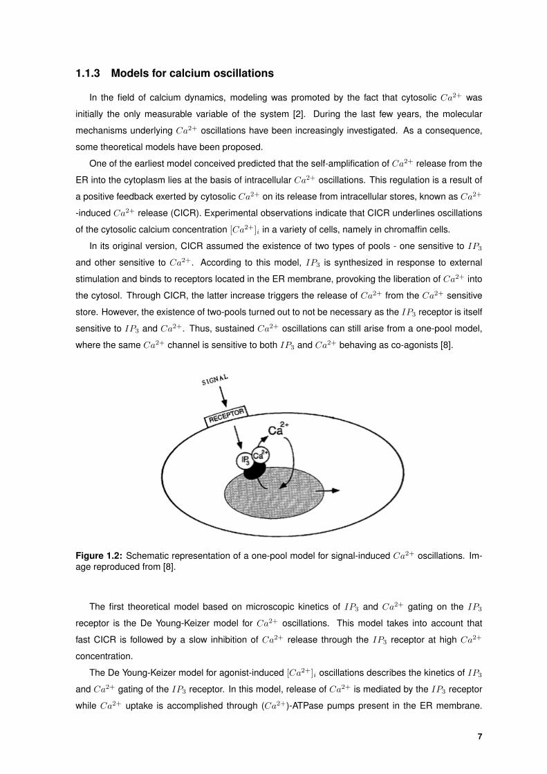
sensitive to IP3 and Ca2+. Thus, sustained Ca2+ oscillations can still arise from a one-pool model,
where the same Ca2+ channel is sensitive to both IP3 and Ca2+ behaving as co-agonists [8].
Figure 1.2: Schematic representation of a one-pool model for signal-induced Ca2+ oscillations. Im-age reproduced from [8].
The first theoretical model based on microscopic kinetics of IP3 and Ca2+ gating on the IP3
receptor is the De Young-Keizer model for Ca2+ oscillations. This model takes into account that
fast CICR is followed by a slow inhibition of Ca2+ release through the IP3 receptor at high Ca2+
concentration.
The De Young-Keizer model for agonist-induced [Ca2+]i oscillations describes the kinetics of IP3
and Ca2+ gating of the IP3 receptor. In this model, release of Ca2+ is mediated by the IP3 receptor
while Ca2+ uptake is accomplished through (Ca2+)-ATPase pumps present in the ER membrane.
7

One IP3 receptor is composed by 4 subunits. The gating model assumes the existence of three
binding sites on each subunit of the IP3 receptor: one for IP3 and two for Ca2+ which include an
activation and an inactivation site. Thus, each IP3 receptor subunit, Sijk, is assumed to have three
distinct binding sites: one activation binding site for IP3, one activation binding site for Ca2+ and one
inactivation binding site for Ca2+ which are labeled, respectively, by the first (i), the second (j) and
the third subscript (k). An empty site is denoted by ′0′ and an occupied site by ′1′. A subunit is in
an open state when it has the activation binding site of the IP3 and of the Ca2+ occupied and the
inactivation binding site of the Ca2+ empty, and it is said to be in the state S110. When analyzing the
dynamics of the IP3 receptor, the different subunit states can be represented in terms of xijk =[Sijk]ST
(with∑
i,j,k xijk = 1), which is the fraction of IP3 receptors in the state characterized by the subscript′ijk′. ST is the total amount of subunits.
Figure 1.3: Schematic representation of the channel gating kinetics of the De Young-Keizer modelwith the possible states of one subunit, Sijk. The rate at which the activation binding site of IP3, i,changes from occupied (empty) to empty (occupied) is α, the changing rate of the activation, j, andinactivation binding site of Ca2+, k, is β and γ. Image reproduced from [9]
The model assumes that Ca2+ passes through the IP3 receptor only when three subunits are in
8

the state x110. Thus, the opening probability of the receptor is x3110. One of the key properties used
in formulating models of the IP3 receptor is the experimental analysis of the open channel probability
as a function of [Ca2+]i. Bezprozvanny et al. [10] showed that this open probability is a bell-shaped
function of cytosolic Ca2+. Thus, at low [Ca2+]i an increase in [Ca2+]i increases the open probability
of the receptor, while at high [Ca2+]i an increase in [Ca2+]i decreases the open probability (Figure
1.4).
Figure 1.4: Steady state open probability of the IP3 receptor as a function of cytosolic calciumconcentration, [Ca2+]i, from the DYK model for three different IP3 concentrations. The receptor isactivated quickly by Ca2+ but inactivated by Ca2+ on a slower time scale. This characteristic isincorporated in the magnitude of the rate constants β and γ. Image reproduced from De Young andKeizer, 1992.
The De Young-Keizer model is a nine-variable model that, while unique in giving detailed gating
kinetics, depends on a relatively high number of variables. On the construction of a new model that
describes the non-linear dynamics of calcium in chromaffin cells, a simplified version of the De Young-
Keizer model will be used, the Li-Rinzel model. By exploiting the time scale difference between the
fast activation and slow inactivation of the IP3 receptor by Ca2+ as found in experiments [11], Li and
Rinzel reduced the nine-variable De Young-Keizer model to a two-variable system [9].
This means that, using a multiple time scales method, the De Young-Keizer model is reduced to
a two-variable system, the Li-Rinzel model. The Li-Rinzel model consists of a two equations model
that describes the dynamics of IP3 receptor-mediated [Ca2+]i oscillations, and it is represented by
the following equations
d[Ca2+]idt
= (c1v1w3∞p
3([Ca2+]ER − [Ca2+]i)︸ ︷︷ ︸receptor flux
+ c1v2([Ca2+]ER − [Ca2+]i)︸ ︷︷ ︸leakage flux
− v3[Ca2+]2ik23 + [Ca2+]2i︸ ︷︷ ︸
pump flux
(1.1)
dp
dt=p∞ − p
τp(1.2)
9

where c1 is volume ratio between the ER and the cytosol, v1, v2 and v3 are, respectively, the
maximum IP3-gated, an IP3 - independent leakage permeabilities, and maximum pump rate; p is the
fraction of channels not yet inactivated by Ca2+ (= x000 + x100 + x010 + x110 ), k3 is the dissociation
constant of Ca2+ to the pump, and where
w∞ =
([IP3]
[IP3] + d1
)([Ca2+]i
[Ca2+]i + d5
)τp =
1
a2(Q2 + [Ca2+]i)
p∞ =Q2
Q2 + [Ca2+]i
Q2 = d2[IP3] + d1[IP3] + d3
where d1 is the threshold value for activation of IP3 receptor by IP3, d2 is the threshold inactivation
by Ca2+ of IP3 receptor when IP3 is bound, d3 is the threshold inactivation by Ca2+ when there is
no IP3 bound to the receptor, d5 is the threshold activation by Ca2+ and a2 is the binding rate of
Ca2+ to the inhibiting site of the IP3 receptor. The first term in equation 1.1 describes the Ca2+
flux through the IP3 receptor, and it is proportional to the concentration difference between the ER
and the cytosol. The fraction of open channels is given by w3∞p
3, conserving the same form as the
original model (x3110). Then, the bell-shaped channel opening curve at steady-state (Figure 1.4) can
be understood as the ’weighing’ between a sigmoid activation w3∞ and inactivation curve p3∞. The last
term of equation 1.2 describes the action of Ca2+ ATPase pumps that pump Ca2+ from the cytosol
into the ER. It is important to mention that this model considers that the IP3 receptors are uniformly
distributed along the ER membrane which, even though is an acceptable explanation, it does not
correspond to the true: the IP3 receptors are localized in the membrane of the ER. The Li-Rinzel
model is described and analyzed in more detail in section 2.
1.2 Electrical Properties of the Cell Membrane
Every living cell has a plasma membrane. The cell membrane is selectively permeable, only
allowing certain ions to pass through it, and it controls the flux of ions in and out of the cell, maintaining
a difference of ions concentration between the extra and intracellular medium. This disparity gives
rise to a potential difference across the membrane. Under resting conditions, this potential remains
approximately constant, around -70 mV. This voltage, characteristic to each cell type, is called resting
potential. However, in some cells that are called ’electrically excitable’, the potential can change when
the cell is submitted to an external stimulus.
As mentioned before, an external stimulus may provoke the opening of Ca2+ channels in the
cell membrane, which grants the entry of Ca2+ from the extracellular medium into the cell. This
phenomenon can be better understood by studying the electrical properties of the cell membrane and
the models for membrane potentials.
10

1.2.1 Chromaffin cells are excitable cells
All cells have a resting potential that arises from an electrical charge gradient across the plasma
membrane when the cell is under no external stimulation. A resting potential of - 70 mV means that
the potential inside the cell membrane is about - 70 mV relative to the surrounding medium (which
is defined to be 0 mV), and the cell is said to be polarized. This situation changes when the cell
is subjected to an external stimulus. Depending on how cells respond to this stimulus they can be
considered excitable or non-excitable cells.
If a current is applied for a short period of time in a non-excitable cell, the membrane potential
changes, but it returns directly to its equilibrium value after the applied current is removed. On the
other hand, for excitable cells, if the applied current is sufficiently strong, the membrane potential
exhibits a large excursion towards higher voltages called action potential, in a non-linear manner.
Chromaffin cells are excitable cells [12].
Many cells use the membrane potential as a signal to operate different functions. In the case
of chromaffin cells, the electrical behavior of the cell membrane influences Ca2+ entry and, as a
consequence, catecholamines release, among which adrenaline.
The electrical activity of excitable cells has its origin in the property of proteins composing the
cell membrane - which include channels and transporters - to control the passage of ions across the
membrane.
1.2.2 The origin of membrane potential
The cell membrane provides a boundary separating the interior of the cell from its external envi-
ronment. This membrane consists essentially of phospholipids and proteins. The molecular structure
of phospholipids is characterized by the existence of a polar hydrophilic portion connected to two
hydrophobic chains. This particular structure implies that in an aqueous medium these molecules
spontaneously form a bilayer of about 50-100A [13], associating the hydrophobic portions and having
the hydrophilic parts facing the outside. The highly hydrophobic interior of the bilayer is a barrier to
the diffusion of solvated ions. This low diffusion of ions through a phospholipid bilayer results in an
intrinsic high electrical resistivity of the cell membrane. Thus, while some lipid-soluble material with a
low molecular weight can easily pass through the hydrophobic lipid core of the membrane by simple
diffusion, polar substances cannot do so and additional transport mechanisms are necessary to allow
the passage of such substances across the plasma membrane. As a result, the cell membrane is
said to be selectively permeable.
The transport across cell membranes is orchestrated by specific protein domains embedded in
the cell membrane, such as ion channels and transporters. Ion channels provide mechanisms of
entry/exit of ions following concentration gradients without energy input, whereas transporters can
move ions against concentration gradients with or without energy expenses.
11

Figure 1.5: Schematic view of the cell membrane and the different mechanisms of ionic transport.Some ions are passively transported through ion channels and transporters according to their con-centration gradient, or they are actively transported through transporters against their concentrationgradient, resorting to the use of energy. Image reproduced from [14]
If the membrane is selectively permeable to a certain specie of positively charged ions, these
ions can cross the cell membrane according to their gradient concentration, leaving behind uncom-
pensated negative charges (Figure 1.6). This separation of charges and consequent concentration
gradient gives raise to the membrane potential. This means that now the ions are not only in the
presence of a concentration gradient, but also of an electric field.
Figure 1.6: Permeable selectivity of the cell membrane. The system is divided in two homogeneouscompartments, I and II, occupied by a solution of different concentrations (CI < CII ). The twocompartments are separated by a membrane permeable to a certain specie of positively charged ionsbut impermeable to a certain specie of negatively charged ions. Due to the concentration difference,the positive ions diffuse through the membrane into compartment I. Compartments I and II start tobe, respectively, positively and negatively charged. The two solutions behave as two conductors inequilibrium with electrical potentials VI and VII , and their respective excess charges will be locatedon either side of the membrane, giving rise to a potential VI − VII > 0. Image reproduced from [14]
12
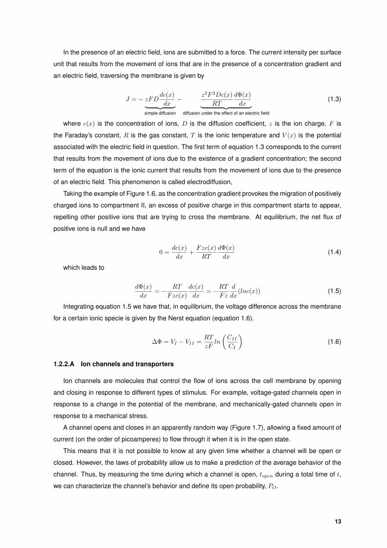
In the presence of an electric field, ions are submitted to a force. The current intensity per surface
unit that results from the movement of ions that are in the presence of a concentration gradient and
an electric field, traversing the membrane is given by
J = − zFDdc(x)
dx︸ ︷︷ ︸simple diffusion
− z2F 2Dc(x)
RT
dΦ(x)
dx︸ ︷︷ ︸diffusion under the effect of an electric field
(1.3)
where c(x) is the concentration of ions, D is the diffusion coefficient, z is the ion charge, F is
the Faraday’s constant, R is the gas constant, T is the ionic temperature and V (x) is the potential
associated with the electric field in question. The first term of equation 1.3 corresponds to the current
that results from the movement of ions due to the existence of a gradient concentration; the second
term of the equation is the ionic current that results from the movement of ions due to the presence
of an electric field. This phenomenon is called electrodiffusion,
Taking the example of Figure 1.6, as the concentration gradient provokes the migration of positively
charged ions to compartment II, an excess of positive charge in this compartment starts to appear,
repelling other positive ions that are trying to cross the membrane. At equilibrium, the net flux of
positive ions is null and we have
0 =dc(x)
dx+Fzc(x)
RT
dΦ(x)
dx(1.4)
which leads to
dΦ(x)
dx= − RT
Fzc(x)
dc(x)
dx= −RT
Fz
d
dx(lnc(x)) (1.5)
Integrating equation 1.5 we have that, in equilibrium, the voltage difference across the membrane
for a certain ionic specie is given by the Nerst equation (equation 1.6).
∆Φ = VI − VII =RT
zFln
(CII
CI
)(1.6)
1.2.2.A Ion channels and transporters
Ion channels are molecules that control the flow of ions across the cell membrane by opening
and closing in response to different types of stimulus. For example, voltage-gated channels open in
response to a change in the potential of the membrane, and mechanically-gated channels open in
response to a mechanical stress.
A channel opens and closes in an apparently random way (Figure 1.7), allowing a fixed amount of
current (on the order of picoamperes) to flow through it when it is in the open state.
This means that it is not possible to know at any given time whether a channel will be open or
closed. However, the laws of probability allow us to make a prediction of the average behavior of the
channel. Thus, by measuring the time during which a channel is open, topen during a total time of t,
we can characterize the channel’s behavior and define its open probability, PO.
13

Figure 1.7: A single-channel recording using the patch-clamp technique. The patch-clamp techniqueis a laboratory technique in electrophysiology that allows the record of currents of single ion channels.From Sanchez, Dani, Siemen, and Hille (1986).
PO =topent
(1.7)
This open probability is going to depend on modulating factors of the channels’ activity, like the
transmembrane potential or the presence of a ligand.
When subjecting the membrane to different electrical stimulus and measuring the amplitude of the
currents when the channel opens (Figure 1.8 (a)) we see that the relation between the single channel
current and membrane voltage is a straight line (Figure 1.8 (b)). This means that an open channel
behaves like an ohmic conductor.
(a) (b)
Figure 1.8: Measurement of channel currents in response to different voltage pulses. (a) Recordof a current produced by a channel formed by two molecules inserted in an artificial lipid bilayer inthe absence of transmembrane concentration gradient. We see that the current varies when varyingthe transmembrane potential difference. (b) The current through the open channel obeys Ohm’s law.Image reproduced from [15].
Ion channels have pores with a diameter of 5-8 A that are ion selective. Due to the variety of
pores’ molecular dimension and to the existence of charge distribution on the interior of the walls of
the channels, the pore size will allow to discriminate between different types of ions based on their
size and charge. Some ion channels become active or inactive with changes in membrane potential.
The Ca2+ voltage-gated channels can be low voltage activated (LVA) or high voltage activated (HVA),
14

based on the membrane potential threshold value.
On the other hand, transporters are highly selective proteins, which have binding sites for specific
ions or molecules. Substrate binding is associated with a conformational change such that the bound
substrate molecule, and only that molecule, is transported across the membrane. Transport through
this type of membrane protein domains can be either passive, facilitating the diffusion of a molecule
following its electrochemical gradient, or active, assisting transport against an electrochemical gradi-
ent (Figure 1.6). In the later, work done has energy costs obtained from phosphate release from ATP
by hydrolysis. This mechanism maintains the activity of Ca2+ ATPase pump, that extorts Ca2+ from
the cytoplasm.
The activity of ion channels and transporters generates differences in ion transmembrane concen-
tration originating an accumulation of charge from both sides of the membrane, by electrodiffusion.
The lipid bilayer may therefore be regarded as a capacitor. Moreover, one can think of the cell
membrane as a capacitor in parallel with ionic currents, and can describe the cell membrane as an
electrical circuit.
1.2.3 Equivalent circuit of the cell membrane
The electrical properties of excitable cells can be described in terms of electrical circuits, with each
component of the cell membrane acting as a basic component of an electrical circuit.
The cell membrane forms an insulating barrier separating electrically charged ions, and can be
thought of as a capacitor C in parallel with ionic currents.
Figure 1.9: Comparison of the cell membrane and its equivalent electrical circuit. The ion chan-nels inserted the cell membrane, when open behave as an ohmic conductor. Due to its selectivepermeability, the cell membrane acts as a capacitor.
Due to charge conservation, the electrical activity of the cell membrane can be described by
equation 1.8.
CdV
dt+ I = 0 (1.8)
where I represents the combination of all ionic currents passing through the cell membrane.
15
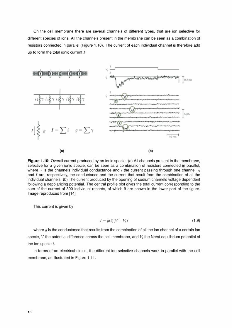
On the cell membrane there are several channels of different types, that are ion selective for
different species of ions. All the channels present in the membrane can be seen as a combination of
resistors connected in parallel (Figure 1.10). The current of each individual channel is therefore add
up to form the total ionic current I.
(a) (b)
Figure 1.10: Overall current produced by an ionic specie. (a) All channels present in the membrane,selective for a given ionic specie, can be seen as a combination of resistors connected in parallel,where γ is the channels individual conductance and i the current passing through one channel, gand I are, respectively, the conductance and the current that result from the combination of all theindividual channels. (b) The current produced by the opening of sodium channels voltage dependentfollowing a depolarizing potential. The central profile plot gives the total current corresponding to thesum of the current of 300 individual records, of which 9 are shown in the lower part of the figure.Image reproduced from [14]
This current is given by
I = g(t)(V − Vi) (1.9)
where g is the conductance that results from the combination of all the ion channel of a certain ion
specie, V the potential difference across the cell membrane, and Vi the Nerst equilibrium potential of
the ion specie i.
In terms of an electrical circuit, the different ion selective channels work in parallel with the cell
membrane, as illustrated in Figure 1.11.
16

Figure 1.11: Equivalent electrical circuit of the cell membrane (Hodgkin and Huxley, 1952). Eachbranch of the electrical circuit represents the contribution to the total transmembrane current from aspecific ion specie channel. In this case, three different type of ion channels are embedded in the cellmembrane, Na+, K+ and a leakage L.
The ion selective permeability of the cell membrane is represented by an electrical circuit com-
posed of a resistance in series with a voltage source equal to the ion equilibrium potential. In turn,
the representative branches of a specific ion specie channel are in parallel with a capacitance.
1.2.4 Models for membrane potential oscillations
The most important and complete work when it comes to the study of generation and propagation
of electrical signals in excitable cells is the work of Alan Hodgkin and Andrew Huxley. They developed
the first quantitative model of the propagation of an electrical signal along an axon, where the ionic
currents involved in the propagation of an action potential in an axon were revealed (K+ and Na+),
as well as the dynamics of its conductances.
They hypothesized the existence of selective ion channels whose opening is dependent on the
membrane potential. This means that the probability of a certain ion channel to be open varies with
the potential of the cell membrane. For example, the opening probability of the K+ channels varies
according to equation 1.10.
dn
dt=n∞(V ) − n
τn(V )(1.10)
where n∞ is the open probability in the stationary state and τn is the characteristic time. The
variable n is also know as the activation variable for the potassium channels. Hodgkin and Huxley
also noticed that, from an experimental point of view, the conductances of the K+ channels vary
according to equation 1.11.
gK(V ) = gKn4 (1.11)
17

where gK is the maximal conductance of the potassium channels, which corresponds to the sit-
uation where all the channels are open. A similar formalism is used to describe the dynamics of the
conductance of the Na+ channel, where we have that the activation and inactivation variables, m and
h, vary according to equation 1.12 and 1.13.
dm
dt=m∞(V ) −m
τm(V )(1.12)
dh
dt=h∞(V ) − h
τh(V )(1.13)
and the conductance gNa varies accordint to equation 1.14
gNa(V ) = gNam3h (1.14)
where gNa is the maximal conductance of the ion channels. The activation and deactivation vari-
ables m and h satisfy a first order transition of the same type as n, and one can write the following
differential equations,
Reminding that an ionic current is of the form I = g(V −Vi), we have that the membrane potential
oscillations in an excitable cell is given by equation 1.15
CdV
dt= −gKn4(V − VK) − gNam
3h(V − VNa) − gL(V − VL) (1.15)
where the last term represents a leakage current, referring to the influence of other currents pass-
ing through the membrane of the cell that are not significant enough to be considered individually.
Equation 1.15 and equations 1.13, 1.12 and 1.10 form the set of the Hodgkin-Huxley equations.
The Hodgkin-Huxley model describes the repetitive firing of action potentials in an axon but it can
be adapted to describe more complex behavior exhibited by other excitable cells.
Many cells’ behavior is characterized by brief bursts of oscillatory activity interspersed with qui-
escent periods during which the membrane potential changes only slowly; this behavior is called
bursting.
Calcium oscillations are modulated inside an electrical model of the cell membrane. Thus, the
Hodgkin-Huxley model can be adapted to describe intracellular Ca2+ oscillations. In particular, the
Gall-Susa model that investigates the role of plasma membrane Na+/Ca2+ in pancreatic β-cells. For
that, it describes intracellular Ca2+ oscillations having into the account the electrical activity of the cell
membrane and its potential variations, which is given by
CdV
dt= −IK − ICa − IK(Ca) (1.16)
dn
dt=n∞(V ) − n
τn(V )(1.17)
18

with
IK = gKn(V − VK)
ICa = gCam∞(V − VCa)
IK(Ca) = gKCa[Ca2+]i(V − VK)
70 + [Ca2+]i
where IK is the delayed rectifier K+ current, ICa is the voltage-dependent L-type (a subtype of
HVA) Ca2+ current, IK(Ca) is the Ca2+ -activated K+ current, and n is the gating variable for the
delayed-rectifier K+ channel. During the bursts, when the L-type Ca2+ channels are open, the Ca2+
is pumped from the cytosol in the ER. This Ca2+ accumulated in the ER is then gradually released in
the cytosol. Equation 1.18 gives us the variation of cytosolic Ca2+ concentration.
d[Ca2+]idt
= −αICa − kCa[Ca2+]i︸ ︷︷ ︸membrane flux
+ krel([Ca2+]ER − [Ca2+]i)︸ ︷︷ ︸
ER flux
− kpump[Ca2+]i︸ ︷︷ ︸ER pump flux
(1.18)
where α is a factor that converts current into concentration changes, kCa is the Ca2+ removal rate
by mechanisms other than sequestration in the ER, krel is the rate of calcium release from the ER
and kpump is the pump activity of the Ca2+ -ATPase in the ER. The last two terms in equation 1.18
are due to the presence of the ER. The evolution equation of calcium concentration in the ER is given
by
d[Ca]retdt
= −krel([Ca]ret − [Ca]i)︸ ︷︷ ︸ER flux
+ kpump[Ca]i︸ ︷︷ ︸ER pump flux
(1.19)
The Gall-Susa model will be described and analyzed in more details in section 2.
19
1.3 Aim of the Work
A diverse range of cellular activities is regulated through calcium signaling. Calcium is an im-
portant intracellular messenger that regulates cellular processes such as gene transcription, muscle
contraction and hormonal secretion. In the case of chromaffin cells, intracellular oscillations of calcium
control the secretion of catecholamines like adrenaline. Because of their wide availability, their ease
of isolation and preparation in primary cultures, and the fact that intracellular Ca2+ oscillations in chro-
maffin cells are produced by the same mechanisms that other secretory cells, chromaffin cells have
been widely used in biochemical and electrophysiological. Plus, chromaffin cells are structurally very
similar to pos-synaptic sympathetic neurons, being also used neuropharmacological studies [17, 18].
Thus, findings on catecholamine release in chromaffin cells can be extrapolated to basic mechanisms
in the central and peripheral nervous system [19]. It may even help to better understand the origin of
certain neurodegenerative diseases, since deregulation of Ca2+ -mediated signaling has been impli-
cated in many neurodegenerative diseases like Alzheimer’s disease [20]. In fact, the ER appears to
be a focal point when it comes to neuronal alterations that result in Alzheimer [21].
It was experimentally observed that the Ca2+ oscillations in chromaffin cells underlying the se-
cretion of catecholamines present two distinct patterns, fast oscillations imposed in a slow oscillating
pattern and fast spiking, which no existing model can explain. Given that all the cells analyzed where
submitted to the same stimulus (100µM of methacoline, a substance that triggers the synthesis of
IP3) and that different patterns of Ca2+ oscillations result in secretion of varying amounts of cat-
echolamines and, consequently, in different functional responses [22]. This puts into evidence the
importance of constructing a new mathematical model that describes the non-linear dynamics of in-
tracellular calcium in chromafin cells and that it is able to reproduce both patterns of oscillations found
experimentally, possibly explaining their existence. The already existing models that describe intra-
cellular Ca2+ oscillations in chromaffin cells fail to reproduce both pattern of oscillations and thus, to
provide an explanation for their existence.
Our aim is to build a biologically-plausible mathematical model able to reproduce the experimental
observations about calcium oscillations in rat chromaffin cells in order to help deciphering why similar
cells under the same conditions present different oscillatory patterns. For that, we will combine two
existing models: Li-Rinzel and Gall-Susa models.
Gall-Susa model describes calcium oscillations taking into account the electrical activity of the
cell membrane, but not the role of the IP3 receptor. On the other hand, Li-Rinzel model describes
calcium oscillations considering the contribution of calcium release from the ER only. Knowing that
both mechanisms play a major role in the regulation of [Ca2+]i, we will incorporate the flux of calcium
passing through the IP3 receptors and ER pumps described in the Li-Rinzel model, into the Gall-Susa
model, thus having a complete mathematical model that describes the non-linear dynamics of Ca2+
in chromaffin cells.
The fact that the Gall-Susa model structure resemblances the structure of Li-Rinzel encourages
the incorporation of one model into the other (both are based on the Hodgkin-Huxley model). Also,
20

both Gall-Susa and Li-Rinzel are simple models, having a small number of variables, which makes it
easy to incorporate one into the other.
We will also compare the behavior of this new model with experimental results of Ca2+ oscillations
in chromaffin cells in the presence of various pharmacological agents that interfere with Ca2+ chan-
nels, and propose some experiments to study the influence of certain parameters in the obtainment
of the different patterns of oscillations observed experimentally.
The new mathematical model we propose to build innovates by its simplicity. We retain only what
we know to be the essential mechanisms to produce intracellular Ca2+ oscillations (the electrical
activity of the cell membrane and the dynamics of the IP3 receptor in the ER). This makes the model
easy to study and to manipulate, and it facilitates future improvements that it may need. Also, it makes
it easier to adapt in order to study other related characteristics of chromaffin cells, serving as a tool for
future studies. As mentioned earlier, there are mathematical models for intracellular Ca2+ oscillations
in chromaffin cells. These models however, don not reproduce the two oscillatory patterns observed
experimentally by Dr. Martınez, and their complexity makes it hard to make the necessary study and
consequent changes to reproduce both patterns and provide an explanation for their existence.
21

22

2Dynamics of theoretical models
The model that will be constructed to study the Ca2+ dynamics in chromaffin cells results from the
coupling between two previously published models: one model that describes the plasma-membrane
Ca2+ dynamics [23] - Gall-Susa model - and another that describes the Ca2+ exchanges between
the endoplasmic reticulum and the cytosol [9] - Li-Rinzel model.
In this section, these two theoretical models - Li-Rinzel and Gall-Susa - will be analyzed. In
particular, we will reproduce some published results that result from the integration of the equations
that describe each model, and present some new ones that will give us a better understanding about
the origin of Ca2+ oscillations according to each model.
23

2.1 Li-Rinzel model
The Li-Rinzel model is a two-variable model that describes the cytosolic Ca2+ dynamics, d[Ca2+]idt ,
taking into account the activation/deactivation dynamics of the IP3 receptors, dpdt . Using the software
XPP and XXP-AUTO (see Appendix A), we reproduced the results published by Li and Rinzel in 1994
(Figure 2.1 and 2.2).
The Li-Rinzel model is composed by the following set of equations:
d[Ca2+]idt
= (c1v1w3∞p
3([Ca2+]ER − [Ca2+]i)︸ ︷︷ ︸receptor flux
+ c1v2([Ca2+]ER − [Ca2+]i)︸ ︷︷ ︸leakage flux
− v3[Ca2+]2ik23 + [Ca2+]2i︸ ︷︷ ︸
pump flux
(2.1)
dp
dt=p∞ − p
τp(2.2)
The first equation describes the Ca2+ exchange between the cytosol and the ER. When the con-
centration of calcium in the endoplasmic reticulum, [Ca2+]ER, is greater than the concentration in the
cytosol, [Ca2+]i, a flux of Ca2+ flows from the interior of the ER into the cytosol through IP3 receptors
present in the ER membrane, described by the first term of equation 2.1. While v1 represents the
rate/permeability of the IP3 receptor, w3∞p
3 represents the probability of the IP3 receptor being open;
more precisely, w3∞ is the probability of the IP3 receptor having the activation binding site of IP3 and
of Ca2+ occupied and p3 is the probability of having the inactivation binding site of Ca2+ empty. This
last one varies according to equation 2.2, where p∞ is the fraction of not inactivated IP3 receptor in
the stationary state.
Besides the flux of Ca2+ that passes through the IP3 receptor, there is also a leakage flux released
from the ER, described by the second term of equation 2.1.
Finally, the last term of equation 2.1 reflects the activity of the ATPase pumps present in the ER
membrane that takes Ca2+ from the cytosol into the ER, against its concentration gradient, at a rate
v3.
This set of equations bears some resemblance with the Hodgkin-Huxley model of the plasma
membrane electrical excitability: instead of the membrane voltage V , we have the cytosolic concen-
tration [Ca2+]i has a major regulator, and instead of the voltage deviation from the Nerst potential
V − Vi we have the concentration gradient [Ca2+]ER − [Ca2+]i as the driving force. Plus, in both
models channel activation and inactivation appear as separate factors with first-order gating kinetics
(dndt , dmdt and dh
dt in the Hodgkin-Huxley model and dpdt in the Li-Rinzel model).
Analyzing Figures 2.1 (a) and (b) we see that the concentration of calcium in the cytosol [Ca2+]i
reaches its maximal value shortly after the maximum of p, which is consistent with what is expected
since the more IP3 receptors are in a non-inactivated state, the bigger is the probability of these
receptors to be open allowing Ca2+ to flow through it and increasing the concentration of calcium in
the cytosol [Ca2+]i.
24

(a)
(b)
Figure 2.1: Reproduction of the time course of p, (a), and of [Ca2+]i, (b), for the Li-Rinzel model.Computed solutions of equations 2.1 and 2.2[9].
25

The periodic oscillations observed in Figure 2.1 do not occur for all concentration of IP3 in the
cytosol [IP3]. The bifurcation diagram of the Li-Rinzel model as a function of [IP3] is shown in Figure
2.2.
Figure 2.2: Bifurcation diagram of the Li-Rinzel model as a function of [IP3]. Reproduction of theresults obtained for the two-variable Li and Rinzel’s model, where we have good agreement of thebifurcation diagram, and thus of the oscillatory response, for the two versions of the model - theoriginal 9-variable and the reduced 2-variable model. The numerical simulations represented in figure2.1(a) and (b) are situated, in the bifurcation diagram, in the zone denoted by the red-dotted line. Wecan see that we are in a stable periodic orbit and we have calcium oscillations. Parameter valuesused for the construction of the bifurcation diagram are given in [9].
For small and big values of [IP3] the system is in a stable steady state and we do not have calcium
oscillations. There is however a stable periodic zone, limited by two Hopf bifurcation points, HB1 and
HB2. In our simulation, [IP3] = 0.4 (red-dotted line in figure 2.2 ) and the system is in a stable
periodic orbit and we have sustained Ca2+ oscillations. It only makes sense to study the behavior
of the system as [IP3] changes since all the other parameters that compose the Li-Rinzel model are
parameters characteristic of the cell and thus, do not change for a same cell, while the the value of
[IP3] can change according to the intensity and frequency of an external stimulus that generates its
production.
26

2.2 Gall-Susa model
The mathematical description of Gall-Susa model is an adapted and expanded version of the
Hodgkin-Huxley model. It takes into consideration the electrical activity of the cell membrane and the
intracellular calcium dynamics. The model is described by the following set of equations:
CdV
dt= −IK − ICa − IK(Ca) (2.3)
dn
dt=n∞(V ) − n
τn(V )(2.4)
d[Ca2+]idt
= −αICa − kCa[Ca2+]i︸ ︷︷ ︸membrane flux
+ krel([Ca2+]ER − [Ca2+]i)︸ ︷︷ ︸
ER flux
− kpump[Ca2+]i︸ ︷︷ ︸ER pump flux
(2.5)
d[Ca]ER
dt= −krel([Ca]ER − [Ca]i)︸ ︷︷ ︸
ER flux
+ kpump[Ca]i︸ ︷︷ ︸ER pump flux
(2.6)
Equation 2.3 describes how the potential of the cell membrane varies as different ion currents
pass through it. Even though there are more currents crossing the cell membrane, this model only
takes into account the potassium current passing through voltage-gated K+ channels and through
Ca2+- activatedK+ channels - IK and IK(Ca), respectively -, and the calcium current passing through
voltage-gated Ca2+ channels.
Similarly to what was seen in the Hodgkin-Huxley model, each ion channel has a certain probability
of being in the activated and in the inactivated state. As already explained in the Introduction, this
probabilities vary with the cell membrane potential. The probability corresponding to the dynamics
of the voltage-gated calcium channels and to the Ca2+-activated K+ channels is very fast when
compared to the one of the voltage-gated potassium channels. Thus, we only have an evolution
equation for the gating variable for the K+ current, n, and the gating variables for the other currents
are considered instantaneous.
Equation 2.5 describes how the concentration of free cytosolic calcium varies as Ca2+ passes
through the cell membrane and through the ER membrane. Through the cell membrane, we have the
calcium current passing through voltage-gated Ca2+ channels that it is going to reflect in an increase
of [Ca2+]i (αICa); on the other hand, we have Ca2+ being pumped out of the cell by ATPase pumps
present in the membrane that work against its concentration gradient (kCa[Ca2+]i), contributing to
the decrease of [Ca2+]i. Besides this, there are Ca2+ exchanges between the cytosol and the ER -
last two terms of equation 2.5 and equation2.6. When [Ca2+]ER is bigger than [Ca2+]i, a leakage of
Ca2+ starts to flow according to its concentration gradient, krel([Ca2+]ER − [Ca2+]i), while there is
Ca2+ constantly being pumped from the cytosol into the ER by ATPases present in the ER membrane,
kpump[Ca2+]i.
The original Gall-Susa model, published in 1999, also considered the present of aNa+-dependent
Ca2+ current - INa/Ca - that we chose not to use since this current caused no significant difference
in the bursting mechanism and thus, in the electrical activity of the cell [23]. This way, we have a
simple model that with a small number of variables is able to describe the bursting that results from
27

the electrical activity of the cell.
Using XPP to numerically integrate equations 2.3- 2.6, we reproduced the results obtain by Gall
and Susa (model III of [23]) in terms of cytosolic calcium dynamics. The results are illustrated in
Figure 2.3.
(a)
(b)
28

(c)
(d)
Figure 2.3: Reproduction of the time courses of the gating variable for voltage-gated K+ channels, n,the electrical activity, V , and calcium concentrations in the cytosol, [Ca2+]i, and in the ER, [Ca2+]ER,for the Gall and Susa model. Numerical solutions of equations 2.3, 2.4, 3.7 and 2.6[23].
The time course of the membrane potential V (Figure 2.3 (b)) exhibits spikes of approximately con-
stant amplitude (∼ 25 mV). This fast spiking is followed by a silent phase where V slowly increases,
and we have bursting.
The dynamics of [Ca2+]i (Figure 2.3 (c)) is almost as fast as the dynamics of V , following the
29

same pattern of fast spiking followed by a slow increase of the variable; the bursting oscillations in the
voltage are mirrored by bursting oscillations in cytosolic Ca2+ concentration.
On the other hand, [Ca2+]ER follows a much slower dynamic, slowly increasing during the active
phase and slowly decreases during the silent phase. This becomes clear when we overlap the two
graphs, V and [Ca2+]ER.
Figure 2.4: Overlap of the graphs for the membrane potential V and the calcium concentration in theER [Ca2+]ER. The concentration of Ca2+ in the ER slowly increases during the active phase of V ,and slowly decreases during the silent phase.
Exploiting the time scale difference that exists between the dynamics of the variables of the system
will help us to describe and interpret, in a simple manner, the behavior of the full model.
Rinzel (1985) used this approach to exploit the control mechanism of bursting in excitable cells
by studying how the slow behavior of intracellular Ca2+ influences the generation of fast spikes [24].
Mathematically, this is equivalent to consider a fast subsystem with the slow variable as a parameter,
which in the case of the model in study is [Ca2+]ER. We can reduce Gall-Susa 4-variable model
(V, n, [Ca2+]i, [Ca2+]ER) to a 3-variable fast subsystem (V, n, [Ca2+]i) with a slow variable [Ca2+]ER.
Our analysis, begins by treating the slowly varying quantity [Ca2+]ER as a parameter. We start
by studying the simple case in which no spikes occur during the active phase. We generate such
behavior in our model by imposing the instantaneous variation of n with V . This means that n reaches
its steady state n∞ instantaneously. To simulate this behavior, we consider n = n∞ and the evolution
equation for n disappears (n is now treated as a parameter), reducing Gall-Susa fast subsystem to a
2-variable system (V, [Ca2+]i).
30

Figure 2.5: Time course of V for the reduced 2-variable fast subsystem of Gall-Susa model(V ,[Ca2+]i) with the gating variable n and [Ca2+]ER as parameters. By considering the instantaneousadaption of n to the voltage V , the spikes in the active phase of bursting disappear.
Figure 2.6: Bifurcation diagram of the reduced 2-variable fast subsystem of Gall-Susa model(V ,[Ca2+]i) with the slow variable [Ca2+]ER as a bifurcation parameter
The Z-shaped curve in Figure 2.6 is the V-nullcline of the fast subsystem. In other words, it
corresponds to the values of V for which the total current passing through the cell membrane I =
IK + IK(Ca) + ICa is null, which corresponds to a steady state. The upper and lower branches of this
31

curve correspond to stable steady states, while the intermediate branch (dashed line) corresponds to
unstable steady states. We can see that the slow dynamics of [Ca2+]ER causes a switch between the
upper and lower steady state.
If we now take into consideration the delay in the adaptation of n to V , we have a fast subsystem
of 3-variables (V, n, [Ca2+]i) with [Ca2+]ER as a variable. The bifurcation diagram of such a system is
plotted in Figure 2.7.
Figure 2.7: Sketch of the bifurcation diagram of the Gall-Susa model for β cells, with [Ca2+]ER as thebifurcation parameter. The Z-shaped curve denotes the steady states of V as a function of [Ca2+]ER.A solid line indicates a stable steady state, and a dashed line indicates an unstable steady state. Thetwo branches denote the maximum and minimum of V over one oscillatory cycle. HB denotes a Hopfbifurcation point. A burst cycle of the full model (equations 1.31-1.34) is projected, in blue, on the (V,[Ca2+]ER) plane. (Results obtained with XPP-AUTO).
For increasing values of [Ca2+]ER, a stable steady state looses its stability through a Hopf bifur-
cation. The stable limit cycle then looses its stability through an homoclinic bifurcation. After this
bifurcation, a stable steady state corresponding to a low voltage is established.
If now we couple the dynamics of the fast subsystem to the slower dynamics of [Ca2+]ER, we
obtain the burst cycle for the full model (represented by the blue line of Figure 2.7). The behavior of
the full system can be understood as slow variations of the fast subsystem.
When the system is in a periodic stable state, it is in repetitive spiking mode (active phase). At
this point, the voltage-gated Ca2+ channels are open and calcium is entering the cell, which makes
the cytosolic Ca2+ concentration increase and, consequently, the Ca2+ concentration in the ER. The
entry of Ca2+ in the cytosol increases the number of open Ca2+ -activated K+channels. The opening
of this channels will provoke the exit of positively charged ions (K+) from the intracellular medium,
which is going to repolarize the cell membrane and the resting potential is restored (low branch of
stable steady state in Figure 2.7). At the resting potential, the Ca2+ channels are closed, the entry of
32

Ca2+, which are positively charged ions, into the cell stops. The membrane potential starts to slowly
increase as Ca2+ is release into the cytosol from the ER (silent phase). The membrane potential
increases until a value for which the voltage-gated Ca2+ channels open again completing the cycle.
It is now clear that the slow dynamics of [Ca2+]ER causes the switch between spiking (active
phase) and a steady state behavior (silent phase). The length of the burst is determined by the am-
plitude of the [Ca2+]ER oscillations (the burst cycle is limited by [Ca2+]ER = 154µM and [Ca2+]ER =
167µM ).
This allows us to conclude that there are two oscillatory processes interacting to make bursting: a
fast oscillation in V imposed on a slower oscillation in [Ca2+]ER.
33

34

3A new model for Ca2+ oscillations in
chromaffin cells
As mentioned before, our goal is to construct a new model for the intracellular calcium dynamics
in chromaffin cells, by coupling the Gall-Susa and the Li-Rinzel models. This requires an adaptation
of the models as they are put together, to ensure that their dynamics remain approximately the same
as new variables are added. Namely, Gall-Susa model will have to undergo some changes as terms
of Li-Rinzel model are added to it.
In this section, it will be explained in more detail what changes to the models we had to make and
why. We will also present an analysis and qualitative viewpoint of bursting in chromaffin cells using
the same method as for Gall-Susa model, and we will exploit the behavior of the new constructed
model by trying to reproduce some experimental observations; particularly we will study how the
model behaves in the presence of pharmacological agents that inhibit the activity of the IP3 receptor.
Finally, we will propose a reasonable testable explanation for the existence of different types of
oscillations observed in chromaffin cells.
35

3.1 New model
Gall-Susa model describes the dynamics of intracellular Ca2+ having into account the exchange
of Ca2+ between the extracellular medium and the cytosol. The voltage-gated Ca2+ channels open
and close in response to the electrical activity of the cell membrane.
Figure 3.1: Experimental observations where the electrical activity of the cell membrane V is mea-sured in parallel with the variation of cytosolic Ca2+. All the significant variations of cytosolic Ca2+
concentration coincide with variations of the membrane potential. The measurement of cytosolic Ca2+
concentration and of the membrane potential where made simultaneously. For this experiment, theonly stimulus to which the cell is submitted are the variations of potential of the cell membrane. Thus,this does not describe a situation where we have Ca2+ oscillations and the secretion of adrenaline.
Figure 3.1 illustrates the relation between the membrane potential of the cell and the cytosolic
concentration of Ca2+.
Gall-Susa model also describes the Ca2+ exchange between the cytosol and the ER, but not
through the IP3 receptor. Instead, it only considers a leakage flux of Ca2+ that passes through
channels present on the ER membrane that play a minor role. It doesn’t account, however, the Ca2+
passing through the IP3 receptors nor their complex dynamics.
Experiments performed by Dr. A. Martınez from the Universidad Autonoma de Madrid show that
in the presence of a pharmacological agent that inhibits the activity of the IP3 receptor, the Ca2+
oscillations disappear. This leads us to the conclusion that the IP3 receptors play a fundamental role
in the generation of cytosolic Ca2+ oscillations.
Unlike Gall-Susa, Li-Rinzel model describes the exchange of Ca2+ between the cytosol and the
ER having into account the flux of Ca2+ that passes through the IP3 receptors. Thus, in order to have
a model that fully describes the intracellular Ca2+ dynamics of chromaffin cells we need to have a
model that describes not only the electrical activity of the cell membrane and the flux of Ca2+ passing
through it but also the flux of Ca2+ passing through the IP3 receptors present in the ER membrane.
36

Figure 3.2: Scheme of fluxes and currents in the cell according to the new model. Present on the cellmembrane are ion channels that allow the entry and exit of ions, namely the entry of Ca2+ into thecell, and ATPases that pump the intracellular Ca2+ outside the cell. This ATPases are also present inthe ER membrane, preventing the cell to reach toxic values of Ca2+. Embedded in the ER membranethere are also the IP3 receptors that, when open allow the passage of Ca2+ from the ER into thecytosol. Image reproduced from [14].
Such model can be built by incorporating the flux of Ca2+ passing through the IP3 receptors of
Li-Rinzel model and the evolution equation describing its dynamics into Gall-Susa model.
In Li-Rinzel model, the flux of calcium through the IP3 receptors is given by
f = c1v1w3∞p
3([Ca2+]ER − [Ca2+]i) (3.1)
while the dynamics of the IP3 receptors is described by the following equation
dp
dt=p∞ − p
τp(3.2)
Adding this two components of the Li-Rinzel model to the Gall-Susa model, we obtain a model
described by the following set of equations
37

dV
dt= − 1
C
(IK + ICa + IK(Ca)
)(3.3)
dn
dt=n∞ − n
τ(3.4)
dp
dt=p∞ − p
τp(3.5)
d[Ca2+]idt
= −αICa − kCa[Ca2+]i︸ ︷︷ ︸membrane flux
+ krel([Ca2+]ER − [Ca2+]i)︸ ︷︷ ︸leakage flux
− c1kpump[Ca2+]i︸ ︷︷ ︸ER pump flux
(3.6)
+ c1v1w3∞p
3([Ca2+]ER − [Ca2+]i)︸ ︷︷ ︸flux trhough the IP3 receptors
(3.7)
d[Ca2+]ER
dt= − 1
c1krel([Ca
2+]ER − [Ca2+]i)︸ ︷︷ ︸leakage flux
+ kpump[Ca2+]i︸ ︷︷ ︸ER pump flux
− c1v1w3∞p
3([Ca2+]ER − [Ca2+]i)︸ ︷︷ ︸flux through the IP3 receptors
(3.8)
Because this set of equations describes variations of Ca2+ concentrations, they must depend on
the volume of the ER and the cytosol. Gall-Susa model assumes that the volume of the ER and the
volume of the cytosol are approximately the same, which is not accurate. The ratio between the ER
and the cytosol is ≈ 20%. Because of this, we also had to add a variable c1(= V olER
V olcytosol) to the terms
of the model corresponding to the Gall-Susa model.
Also, the values of some parameters had to be adjusted so that the order of magnitude of the
fluxes and the dynamics of the channels involved in the exchange of Ca2+ remain roughly the same
in our new model as in the Gall-Susa and Li-Rinzel models.
In particular, we had to change the threshold value of activation of the IP3R by IP3 d1 (from
d1 = 0.13 to d1 = 1), the threshold value for activation of the IP3R by Ca2+ d5 (from d5 = 0.08234 to
d5 = 0.2), the maximum IP3-gated permeability v1 (from v1 = 6s−1 to v1 = 0.45s−1). Although these
values are very different from the ones of the original model (Li-Rinzel model), there is no agreement
on the realistic values for this parameters and so, there is no reason to exclude the values chosen by
us and to not consider them valid.
The value for the rate of Ca2+ pumped out of the cell, kpump, originally used in the Gall and
Susa’s model (kpump = 0.2ms−1) has been modified in agreement with experimental data. We had
to decrease the value of this parameter conserving the behavior of the original model. For that,
the change of kpump (from kpump = 0.2ms−1 to kpump = 0.0589) led to a change of the rate of
Ca2+ release from the ER krel (from krel = 0.0006ms−1 to krel = 0.0002ms−1), of the maximal
conductance of the Ca2+ -activated K+ channels gK(Ca) (gK(Ca) = 30000pS to gK(Ca) = 29000pS),
and the maximal conductance of the K+ channels gK (from gK = 2700pS to gK = 1600pS). As
already referred, the conductance depends on the number of channels existing on the cell membrane.
Considering the order of magnitude of the conductances in study, the decreases performed to their
original values do not reflect on a dramatic change of the number of channels, and thus remain valid.
However, it is important to note that this is merely an estimate having into consideration the values
for the conductances of the ion channels found in literature [23], since there is no way to measure the
conductance of one single channel.
38

All the other values remain the same and were already validated for the publication of the respec-
tive original models, [9] and [23]. The values of all the parameters that are going to incorporate the
new model are listed in Table A.1 (Appendix).
The set of equations 3.3 - 3.8 forms a new mathematical model that describes the non-linear
dynamics of intracellular Ca2+ in chromaffin cells. Equation 3.3 describes the electrical activity of the
cell membrane having into account the contribution of the potassium current K+ from voltage-gated
potassium channels IK and from Ca2+ -activated potassium channels IK(Ca), and the contribution
of the Ca2+ current, ICa. Equation 3.4 and 3.5 describe the dynamics of the gating variable of the
voltage-gated K+ channels and the dynamics of the IP3 receptors, respectively. Equation 3.7 and
3.8 describe the concentration variations of Ca2+ in the cytosol and in the ER, where all the terms of
the evolution equations retain their original significance.
A numerically computed solution was developed for the final cell model, which is shown in figure
3.3.
(a)
39
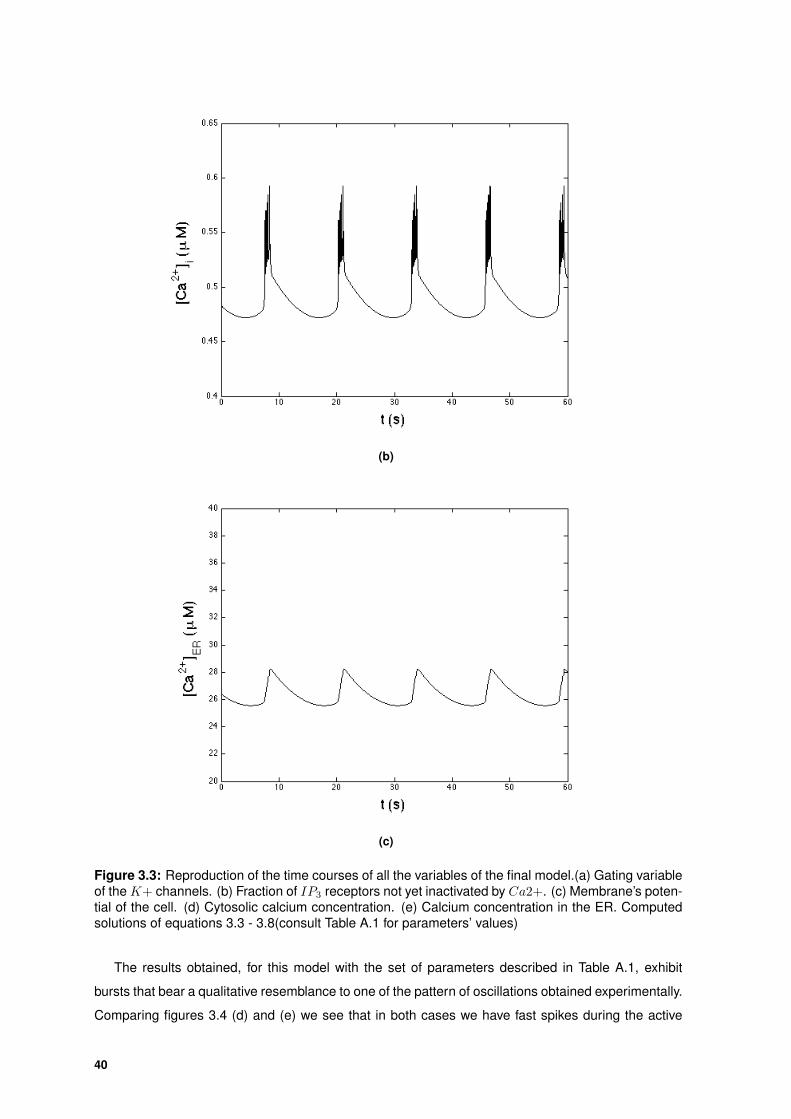
(b)
(c)
Figure 3.3: Reproduction of the time courses of all the variables of the final model.(a) Gating variableof the K+ channels. (b) Fraction of IP3 receptors not yet inactivated by Ca2+. (c) Membrane’s poten-tial of the cell. (d) Cytosolic calcium concentration. (e) Calcium concentration in the ER. Computedsolutions of equations 3.3 - 3.8(consult Table A.1 for parameters’ values)
The results obtained, for this model with the set of parameters described in Table A.1, exhibit
bursts that bear a qualitative resemblance to one of the pattern of oscillations obtained experimentally.
Comparing figures 3.4 (d) and (e) we see that in both cases we have fast spikes during the active
40

phase followed by a gradual decrease in [Ca2+]i.
(d)
(e)
Figure 3.4: Comparison of predict results with experimental results. (d) Intracellular calcium concen-trations, [Ca2+]i, for the final model. (e) Experimental measurements of calcium in rat chromaffin cellsprovided by Dr. A. Martınez, Faculty of Medicine of Universidad Autonoma de Madrid
One can wonder if [Ca2+]ER is the slow variable that controls burst in this full model as well.
The calcium variations in the ER are much slower than the variation of cytoplasmic Ca2+, that varies
almost as quickly as the voltage of the cell membrane.
We start by evaluating the role of this slow variable in bursting by studying the behavior of the
fast subsystem (V ,p,[Ca2+]i), considering n = n∞, like what was done in section 2.2 for the study of
Gall-Susa model.
41

Figure 3.5: Time course of V for the reduced 3-variable fast subsystem of the new model. Byconsidering the instantaneous adaption of n to the voltage V , there are no spikes in the active phaseof bursting.
Like for the Gall-Susa model, by considering the instantaneous adaption of n to the voltage V in
the new model, there are no spikes in the active phase of bursting (Figure 3.5).
In order to study the influence of the slow variable [Ca2+]ER in the passage from the active to the
silent phase in bursting, we plot the bifurcation diagram of the fast subsystem (V, p, [Ca2+]i) with the
slow variable [Ca2+]ER as a bifurcation parameter (Figure 3.6).
Figure 3.6: Bifurcation diagram of the reduced 3-variable fast subsystem of the new model.
42

The Z-shaped curve is the V-nullcline of the fast subsystem (values of V for which the total current
I = IK +IK(Ca)+ICa is null). The upper and lower branches of this curve correspond to stable steady
states, while the intermediate branch correspond to unstable steady states. We can see that the slow
dynamics of [Ca2+]ER causes the switch between the upper and lower steady state.
If we now take into consideration the delay in the adaptation of n to V , we have a fast subsystem
of 4-variables (V, n, p, [Ca2+]i) with [Ca2+]ER as a variable. The bifurcation diagram of such a system
is plotted in Figure 3.7.
Figure 3.7: Sketch of the bifurcation diagram of the final model with [Ca2+]ER as the bifurcationparameter. The Z-shaped curve denotes the steady states of V as a function of [Ca2+]ER. A burstcycle of the full model (equations 3.3 - 3.8) is projected, in blue, on the (V, [Ca2+]ER) plane. Resultsobtained with XPP-AUTO.
Coupling the dynamics of the fast to the slow subsystem, we obtain the burst cycle for the full
model represented in Figure 3.7 by a blue line.
When the system is in a high-V state, the system is in repetitive spiking mode and [Ca2+]ER
increases (active phase); when the system is in a low-V steady state, we are in the silent phase and
[Ca2+]ER decreases. We see that once again the length of the burst is determined by the amplitude
of [Ca2+]ER oscillations and so this variable works as a control mechanism of bursting. In fact, Figure
3.8 makes it clear that the active phase is when [Ca2+]ER slowly increases and the silent phase when
[Ca2+]ER slowly decreases.
43

Figure 3.8: Overlap of the graphs for the membrane potential and the Ca2+ concentration in theER. During the active phase, [Ca2+]ER is slowly increasing, while during the silent phase is slowlydecreasing.
While having a similar shape, the graph of [Ca2+]i according to our new model differs from the
one obtain with Gall-Susa model in the way the silent phase is processed. In the new model, the
silent phase runs for a longer time than in Gall-Susa, which is a consequence of the dynamics of
the IP3 receptors. When the voltage-gated Ca2+ channels close, preventing the entrance of Ca2+
into the cell from the extracellular medium and putting an end to the active phase, there is still a
considerable amount of Ca2+ being release into the cytosol from the ER, passing through the IP3
receptors that remain open for as long as there is Ca2+ enough to bind to the activation binding sites.
Thus, the decrease of [Ca2+]i in the silent phase is less abrupt than in the Gall-Susa model and the
branch corresponding to the silent phase has a small declive, being more similar to the experimental
observations.
44

3.2 Study of the behavior of the model in the presence of phar-macological agents
In one of the experiments performed by Dr. A. Martınez, the calcium dynamics was measured in
the presence of an IP3 channel inhibitor pharmacological agent (2-Aminoethoxydiphenyl borate). It
was observed that after the introduction of the agent in the system, the Ca2+ oscillations ceased.
The equivalent on our mathematical model to inhibiting the IP3 channels is to change the value
of the parameter v1 that scales the number of IP3 channels in the ER membrane. We can study
the effect of variation of v1 in the system through a bifurcation diagram, using v1 as a bifurcation
parameter.
Figure 3.9: Bifurcation diagram of final model with v1 as a bifurcation parameter. For small values ofv1, the system is in a steady state and we have no oscillations of [Ca2+]i.
For small values of v1, the system is in a steady state. From the Hopf bifurcation point HB beyond,
the system is in a periodic oscillatory state, where the amplitude of the oscillations increase as we
increase the value of v1.
Now that we have constructed a mathematical model that describes the non-linear dynamics of in-
tracellular Ca2+ in chromaffin cells, we intend to reproduce some experimental observations. Namely,
we want to know how does our system behave when we inhibit the activity of the IP3 receptors. This
is accomplished by decreasing the value of v1. Figure 3.10 shows what happens when the permeabil-
ity of the IP3 receptors is reduced from 0.45s−1 to 0.1s−1. We see that at the time the value of v1 is
changed, the oscillations cease, which is in qualitative agreement with the experimental observations.
45

(a)
(b)
Figure 3.10: Comparison of the predict results with experimental results when the IP3 channels areinhibited. (a) Experimental measures of intracellular calcium oscillations in the presence of a pharma-cological agent that inhibits the activity of the IP3 channels. We see that when the IP3 channels areinhibited, the calcium oscillations stop. 2-APB 100 µM concerns the pharmacological agents usedto inhibit the IP3 channels. (b) Time evolution of final model when v1 is decreased. At t = 30s, thevariable that regards the number of IP3 channels in the ER is reduced from v1 = 0.45 to v1 = 0.1. Wesee that when we make this change, the calcium oscillations disappear.
46

3.3 Influence of the cell capacitance on the Ca2+ oscillatory pat-terns
As mentioned before, two patterns of oscillations for calcium concentrations were observed exper-
imentally. One type of oscillations was already obtained (Figure 3.4) with the parameters values of
Table A.1.
The main differences between the two oscillation patterns are the frequency and the amplitude
of the oscillations. Comparing the two patterns obtained experimentally we see the second pattern
(Figure 1.1 (b)) has a higher frequency and a smaller amplitude relative to the first (Figure 1.1 (a)). In
an attempt to reproduce the second pattern of oscillations, we changed the values of parameters that
could be the cause for the existence of the two different types of oscillations; namely the capacitance
of the cell membrane (from C = 5310fF to C = 4800fF ).
Figure 3.11: Time course of the intracellular calcium concentrations for the new model with C = 4800.
By decreasing the value of the capacitance, the new model exhibits single spikes with a higher
frequency and smaller amplitude than the pattern previously obtained, in section 3.1. Thus, it retains
the main characteristics of the second pattern obtained experimentally (Figure 3.12).
A decrease of the cell capacity from C = 5310fF to C = 4800fF translates in a decrease of the
cell radius from r = 6.5µm to r = 6.18µm (CA = c where A is the area of the cell 4πr2 and c the
specific capacitance that is 1× 10⁻⁶F ). This presents a possible explanation for the different patterns
of oscillations observed: the sample of chromaffin cells analyzes may have been composed of cells
of different sizes.
47

(a)
(b)
(c)
Figure 3.12: Time evolution of Ca2+ of the final model for two different sets of parameters. (a) Timeevolution of the final model with the value of parameters as described in the Tabel A.1. (b) Timeevolution of the final model with C = 4800fF . When the value of the capacitance C is decreasedfrom 5310fF to 4800fF we obtain an oscillatory pattern with single spikes and, in comparison withthe previous oscillatory pattern obtain, with a higher frequency and a lower amplitude of oscillations.(c) Experimental measurements of calcium in rat chromaffin cells provided by Dr. A. Martınez, Facultyof Medicine of Universidad Autonoma de Madrid
48

4Conclusions and Perspectives
The work developed in this master thesis was set out to build a new mathematical model that
describes the non-linear dynamics of intracellular calcium in chromaffin cells. The motivation behind
the construction of this new model came from the experimental observations of two distinct oscillatory
patterns in chromaffin cells from the same population and submitted to the same conditions, and the
non-existence of a good explanation for this phenomenon. Our goal was to build a model able to
provide such an explanation by reproducing both types of intracellular calcium oscillations observed.
Not only were we able to do that, but we were also able to reproduce some other experimental results
concerning chromaffin cells and their intracellular calcium concentrations, in order to validate our
model.
Calcium oscillations in chromaffin cells are produced by the interplay between the electrical ac-
tivity of the cell membrane and the release of calcium from the endoplasmic reticulum. Thus, our
model needs to have into consideration this two components. To build the new mathematical model
describing the non-linear dynamics of chromaffin cells, we coupled two existing models: one that
describes calcium oscillations cells taking into account the electrical activity of the cell membrane -
Gall-Susa model - and other based on IP3 receptor-mediated calcium oscillations - Li-Rinzel model.
Both these models are an adapted version of the Hodgkin-Huxley model. The Gall-Susa model de-
scribes intracellular calcium variations of concentration using the model of the plasma membrane
electrical excitability of Hodgkin and Huxley to describe the electrical activity of the cell membrane
in pancreatic β-cells. The Li-Rinzel model, even though it does not describe the electrical activity of
the cell has the same structure of the Hodgkin-Huxley model: [Ca2+]i, instead of the voltage V , has
the role of the major regulator of the system, and the concentration difference [Ca2+]ER − [Ca2+]i,
instead of the voltage deviation V − Vi, is the driving force. Thus, both models follow the same struc-
ture, which facilitates the incorporation of one into the other. Plus, Gall-Susa model already takes into
49

account a flux of calcium coming in and out of the ER, which makes it more straight forward to add the
terms from Li-Rinzel corresponding to the IP3 receptor. All this, plus the fact that the Gall-Susa model
describes the calcium concentration in the cytosol as a fast variable, which is in agreement to what
happens in chromaffin cells, makes the coupling of the Li-Rinzel and Gall-Susa models an efficient
way to construct a new mathematical model able to describe the non-linear dynamics of calcium in
chromaffin cells.
There are models that describe the intracellular calcium oscillations in neurons taking into account
the electrical activity of the cell membrane and the dynamics of the IP3 receptors [25,26,27]. The pa-
rameters of these models could be adapted to describe intracellular calcium oscillations in chromaffin
cells. However, these models are very complex, having a high number of variables, which makes it
hard to study them and make any modifications. Plus, they fail to reproduce both patterns of oscil-
lations observed by Dr. Martınez in chromaffin cells and the intracellular calcium dynamics that they
describe does not correspond to the one observed in chromaffin cells. For example, they describe a
chaotic bursting patterns of intracellular calcium and they describe the concentration of calcium in the
cytosol as a slow variable.
In order to couple Gall-Susa and Li-Rinzel models, we added the dynamics of the IP3 receptor
h described in the Li-Rinzel model to the Gall-Susa, as well as the Ca2+ flux through it. To do this
without changing its order of magnitude (the Ca2+ flux through IP3R in the new model can not be too
different than the Ca2+ flux through IP3R in the Li-Rinzel model), we had to adapt the value of some
parameters of the original models. Namely, we had to increase the threshold value of activation of the
IP3R by the IP3, d1, increase the threshold value of activation of the IP3R by Ca2+, d5, and decrease
the maximum IP3-gated permeability, v1. There are no experimental evidences of the real values of
these parameters, which makes our values as valid as the ones used in the Li-Rinzel model.
Another adaptation of the model that we had to make concerns the volume ratio of the ER and the
cytosol. Li-Rinzel model takes into account the fact that the ER and the cytosol have different volume
by considering a volume ratio between the ER and the cytosol c1 smaller than one. On the contrary,
in Gall-Susa model the volumes of the ER and the cytosol are considered to be approximately equal.
Moreover, Gall-Susa uses a value for the activity of the ATPase pump in the cell membrane that it is
bigger than what it is considered a realistic value [6]. To make the terms of the Gall-Susa model take
into account the difference in volumes between the ER and the cytosol, and to have a more realistic
value for the pump activity, we had to change some other parameters. Namely, we had to decrease
the rate of Ca2+ pumped out of the cell (kpump), the rate of Ca2+ release from the ER (krel), the
maximal conductance of the Ca2+ -activated K+ channels (gK(Ca)) and the maximal conductance of
the K+ channels (gK). There is no agreement in literature about the real value of the conductances.
Even so, we tried to deviate as less as possible from the values describe in Gall-Susa.
The new model presents, for the values describes in Table A.1 (Appendix), bursting of the cell
membrane potential. The variations in cytosolic Ca2+ concentration are almost as fast as the vari-
ations in potential. On the contrary, the Ca2+ concentration in the ER varies more slowly; it slowly
increases during the active phase and slowly decreases during the silent phase. This dynamical be-
50

havior can be described on an analysis based on the two different time scales occurring in the system:
the fast subsystem composed by V , n, h and [Ca2+]i, and a slow subsystem composed by [Ca2+]ER.
The behavior of the full system can be understood as slow variations of the fast subsystem, which
means that the slow dynamics of the calcium in the ER is what determines the time scale of the bursts.
With the parameters’ values described in Table A.1, we are able to reproduce one of the patterns
- rapid spikes followed by a slow decrease of the calcium concentration. The second pattern of oscil-
lations, simple oscillations with smaller amplitude and higher frequency, was obtained by decreasing
the value of the cell capacitance. The decrease of a cell capacitance is equivalent to a decrease of
its radius. Then, we can predict that the reason why cells of a same population of chromaffin cells
presents two different types of oscillations is because it is composed by cells of different sizes.
Comparing the oscillatory patterns obtained with the new model and the ones obtain experimen-
tally, we see that the time scale of the experimental measurements is much bigger than the one of
our model. This does not invalidate our model given that the time scale of our new mathematical
model is more realistic than the one obtain experimentally. This may be a result of the difficulties
that underlie these type of experimental measurements. Having access to the data corresponding to
these experimental measurements would help to better understand and interpret these experimental
results.
In summary, we have constructed a new model able to reproduce important experimental obser-
vations and that provides a reasonable testable explanation for the existence of the different types
of oscillations observed. However, this model is only a first attempt to reproduce this experimental
results and it has some limitations. In our model we only take into account the Ca2+ being pumped
into the ER and a flux of Ca2+ that it is released into the cytosol through IP3 receptors (besides a
small leakage flux). However, there is an extra Ca2+ flux that we did not take into account: the flux of
Ca2+ being released into the cytosol through the ryanodine receptors present in the ER membrane
[28]. We did not take this extra flux into account in our model because it did not reveal to be essential
to reproduce the two oscillatory patterns, and indeed we manage to reproduce qualitatively both types
of intracellular Ca2+ oscillations and provide a reasonable explanation for their co-existence, which
was our main purpose. Moreover, this model is based on simple existing models for calcium dynamics
and thus, does not take into account the presence of Na+ channels that play a role in the variation
of membrane’s potential in chromaffin cells [29] by allowing the passage of a sodium current through
the cell’s membrane. But once again, we did not yet take this current into consideration because we
wanted to construct a simple model able to describe our observations concerning the intracellular
calcium oscillations so that now it is easier to improve it and manipulate. This way this model serves
not only for the study of intracellular Ca2+ oscillations but may be eventually used, and after making
the necessary adaptations, to study other related phenomenon in chromaffin cells. For example, to
study the secretion of catecholamines in chromaffin cells and how our sympathetic nervous system
responds to it. Chromaffin cells are neuroendocrine cells that are structurally and functionally in close
proximity to post-synaptic sympathetic neurons, which are a part of the sympathetic nervous system.
Thus, a better understanding the mechanisms underlying calcium oscillations in chromaffin cells and
51

how different oscillatory patterns (and their origin) of intracellular calcium influence catecholamines
secretion can contribute to the study of the sympathetic nervous system and it may even give some
enlightenment about the source of nervous system related diseases.
It is important to mention that, in both the Gall-Susa and the Li-Rinzel model, and consequently on
our new model, it is assumed that the cells are equipotential, which is not true. However, we cannot
predict how this would change the intracellular calcium oscillations described by our model.
As mention before, the intracellular Ca2+ oscillations are directly related to the secretion of cat-
echolamines like adrenaline into our bloodstream. In fact, there are several models that study the
relation between different patterns of intracellular calcium (that are obtained when the cells are sub-
mitted to stimulus of different intensities and duration) and the catecholamine release. Thus, the cells
in study, even though they appear to have identical characteristics (apart, according to our conclu-
sion, from the size) provoke different catecholamine releases and consequently different functional
responses. For a future work, it would be interesting to study this aspect in more detail. For example,
find out how different the functional responses that result from the two oscillatory patterns are. Plus,
for the cell population studied 80% of the cells analyzed presented the second type of oscillations,
simple fast spikes with small amplitude, while only 20% presented bursting. It would also be interest-
ing to study what is the balance between the two types of oscillations in a population of cells from
different individuals and, in case it is not approximately the same for all individuals (80% of one type
oscillations and 20% of others like in this case) study how differently their system responds (change
of the hearth beat and of blood pressure, for example) to a same external stimulus.
52

Bibliography
[1] Garcia A. et al. (2006). Calcium Signaling and Exocytosis in Adrenal Chromaffin Cells. Physiol.
Rev. 86: 1093-1131.
[2] Dupont G., Combettes L., Bird G., Putney J. (2011). Calcium oscillations. Cold Spring Harb Per-
spect Biol; 3:a004226
[3] Kong S., Lee C. (1995). The use of Fura 1 for Measurements of Free Calcium Concentration.
Biochemical Education 23(2): 97-98.
[4] Malgaroli A. Fesce R. Meldolesi J. (1990). Spontaneous Ca2+ fluctuations in rat chromaffin
cells do not require inositol 1,4,5-trisphosphate elevations but are generated by a caffeine- and
ryanodine-sensitive intracellular Ca2+ store. Biol. Chem. 265: 3005-3008
[5] Sneyd J. (2002). An introduction to mathematical modeling in physiology, cell biology, and im-
munology. Proceedings of Symposia in Applied Mathematics 59
[6] Keener J., Sneyd J.(2010). Mathematical Physiology. Springer, New York
[7] Goldbeter A. Dupont G. Berridge MJ. (1990). Minimal model for signal-induced Ca2+ oscillations
and for their frequency encoding through protein phosphorylation. Proc. Natl. Acad. Sci. USA. 87:
1461-1465
[8] Dupont G., Goldbeter A. (1993)One-pool model for Ca2+ oscillations involving Ca2+ and inositol
1,4,5-trisphosphate as co-agonists for Ca2+ release. Cell Calcium. 14: 311-322
[9] Li Y., Rinzel J. (1994). Equations for InsP3 receptor-mediated [Ca2+]i oscillations derived from a
detailed kinetic model: a Hodgkin-Huxley like formalism. J. theor. Biol. 166: 461-473
[10] Bezprozvanny I., J. Watras and B.E. Ehrlich.(1991). Bell-shaped calcium-response curves of
InsP (1, 4, 5)P3 and calcium-gated channels from endoplasmic reticulum of cerebellum. Nature
351: 751-754
[11] Parker I., Ivorra I. (1990).Inhibition of Ca2+ of inositol trisphosphate-mediated Ca2+ liberation: a
possible mechanism for oscillatory release of Ca2+. Proc. Natl. Acad. USA 87 (1): 260-4
[12] Brandt B., Hagiwara S., Kidokoro Y., Miyazaki S. (1976). Action potentials in the rat chromaffin
cell and effects of acetylcholine. J. Physiol. 263(3): 417-439
53
[13] Esteban-Martın S. and Salgado J. (2007). Self-Assembling of Peptide/Membrane Complexes by
Atomistic Molecular Dynamics Simulations. Biophysical Journal vol. 92 3: 903-912
[14] Gall D. (2014). Elements de Biophysique et Physiologie des Cellules Excitables.
[15] Kandel E.R., Schwartz J.H. and Jessel T.M. (2000). Principles of Neural Science. Prentice Hall,
Ltd.
[16] Lodish H., Berk A., Zipursky S., Matsudaira P., Baltimore D., Darnell J. (2000). Molecular Cell
Biology. W. H. Freeman, New York
[17] Shtukmaster S., Schier M., Huber K., Krispin S., Kalcheim C. and Unsicker K. (2013). Sympa-
thetic neurons and chromaffin cells share a common progenitor in the neural crest in vivo. Neural
Development 8: 12.
[18] Morgan A., Burgoyne RD. (1997). Common mechanisms for regulated exocytosis in the chro-
maffin cell and the synapse. Semin. Cell Dev. Biol. 8(2): 141-9.
[19] Garcıa A., Garcıa-De-Diego A., Gandıa L., Borges R. and Garcıa-Sancho J. (2006). Calcium
Signaling and Exocytosis in Adrenal Chromaffin Cells. Physiological Reviews vol. 86 nAo. 4: 1093-
1131.
[20] Woods NK, Padmanabhan J. (2012). Neuronal Calcium Signaling and Alzheimer’s Disease. Adv.
Exp. Med. Biol. 740: 1193-217.
[21] Mattson MP., Gary D.S., Chan S.L. and Duan W. (2001). Perturbed endoplasmic reticulum func-
tion, synaptic apoptosis and the pathogenesis of Alzheimer’s disease. Biochem. Soc. Symp. 67:
151-62.
[22] Stauderman K., Murawsky M. and Pruss R. (1990). Agonist-dependent patterns of cytosolic
Ca2+ changes in single bovine adrenal chromaffin cells: relationship to catecholamine release.
Cell Regul. 1(9): 683-691.
[23] Gall D., Susa I. (1999).Effect of Na/Ca exchange on plateau fraction and [Ca2+]i in models for
bursting in pancreatic β-cells. Biophysical Journal 77: 45-53
[24] Rinzel J. (1985). Bursting oscillations in an excitable membrane model . In B.D. Sleeman and
R.J. Jarvis, editors, Ordinary and partial differential equations, volume 1151 of Lecture Notes in
Mathematics, pages 304-316. Springer, New York.
[25] Falcke M., Huerta R., Rabinovich M. I., Abarbanel H., Elson R., Selverston A. (2000).Modeling
observed chaotic oscillations in bursting neurons: the role of calcium dynamics and IP3. Biol.
Cybern. 82: 517-527.
[26] Ye J., Rozdeba P., Morone U. (2014). Estimating the biophysical properties of neurons with
intracellular calcium dynamics. Physical Review E 89: 062714.
54

[27] Sherman A. and Bertram R. (2004). A calcium-based phantom bursting model for pancreatic
islets. Bull Math Biol. 66(5):1313-44.
[28] Ruiz A., Matute C. and Alberdi E. (2009). Endoplasmic reticulum Ca2+ release through ryanodine
and IP3 receptors contributes to neuronal excitotoxicity.Cell Calcium 46: 273-281.
[29] Vandael D., Ottaviani M., Legros C., Lefort C., Guerineau N., Allio A., Carabelli V. and Carbone
E. (2015). Reduced availability of voltage-gated sodium channels by depolarization or blockade by
tetrodotoxin boosts burst firing and catecholamine release in mouse chromaffin cells. J. Physiol.
593.4: 905-927.
[30] Warashina A., Ogura T. and Inoue M. (2004). A chromaffin cell model to simulate calcium dy-
namics and secretory responses in various conditions. Cell Biology of Chromaffin Cell: 203-210.
[31] Hodgkin A. and Huxley A. (1952). Currents carried by sodium and potassium ions through the
membrane of the giant axon of Loligo. J. Physiol. 116: 449-472
[32] Ermentrout B. (2002).Solving and analyzing dynamical systems using xppaut. Computational
Cell Biology. Springer-Verlag, New York.
[33] De Young G. and Keizer J. (1992). A single-pool inositol 1,4,5-trisphosphate-receptor-based
model for agonist-stimulated oscillations in Ca2+ concentration. Proc. Natl. Acad. Sci. U.S.A. 89:
9895-9899.
[34] Swillens S., Dupont G., Combettes L. and Champell P. (1999). From calcium blips to calcium
puffs: Theoretical analysis of the requirements for interchannel communication. PNS vol. 96 nAo.
24: 13750-13755.
55

56

AAppendix A
A-1
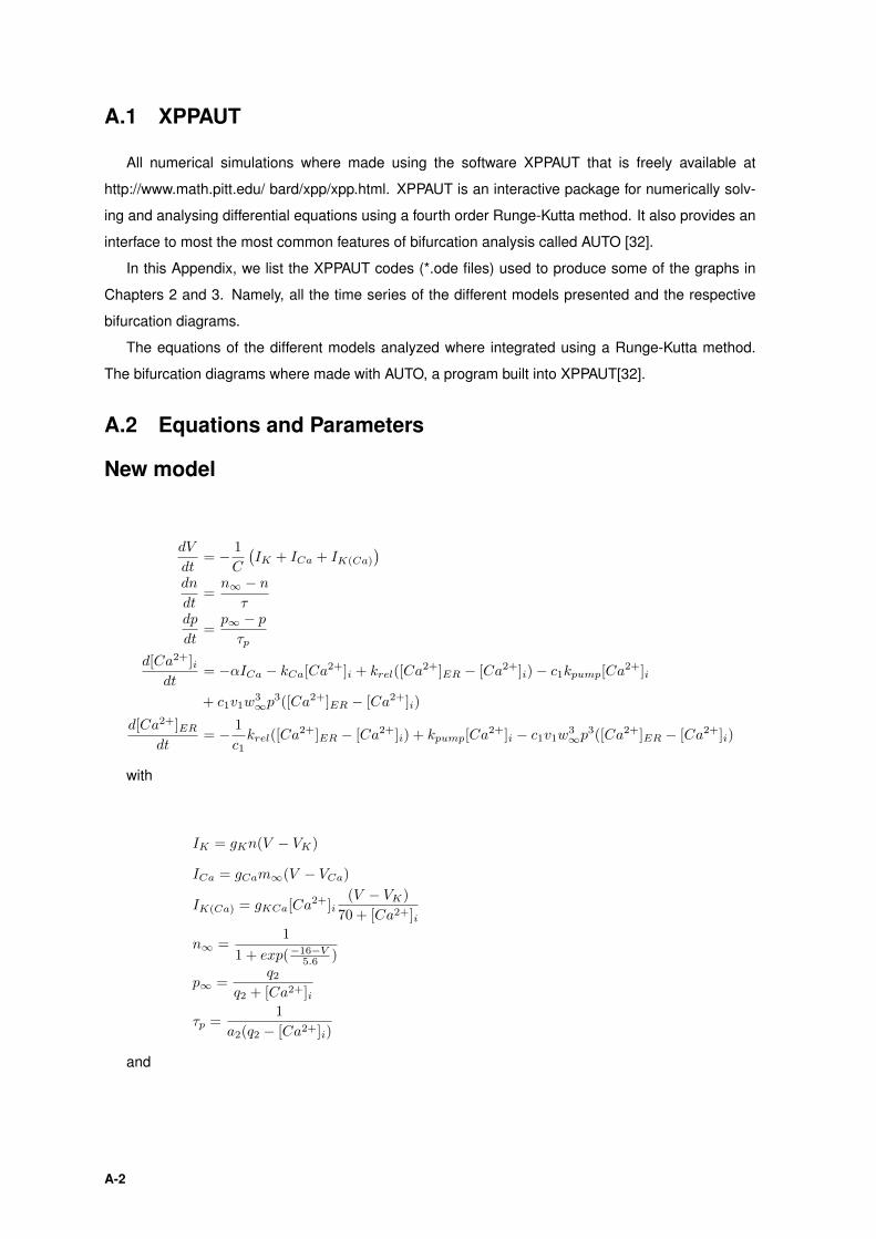
A.1 XPPAUT
All numerical simulations where made using the software XPPAUT that is freely available at
http://www.math.pitt.edu/ bard/xpp/xpp.html. XPPAUT is an interactive package for numerically solv-
ing and analysing differential equations using a fourth order Runge-Kutta method. It also provides an
interface to most the most common features of bifurcation analysis called AUTO [32].
In this Appendix, we list the XPPAUT codes (*.ode files) used to produce some of the graphs in
Chapters 2 and 3. Namely, all the time series of the different models presented and the respective
bifurcation diagrams.
The equations of the different models analyzed where integrated using a Runge-Kutta method.
The bifurcation diagrams where made with AUTO, a program built into XPPAUT[32].
A.2 Equations and Parameters
New model
dV
dt= − 1
C
(IK + ICa + IK(Ca)
)dn
dt=n∞ − n
τdp
dt=p∞ − p
τp
d[Ca2+]idt
= −αICa − kCa[Ca2+]i + krel([Ca2+]ER − [Ca2+]i) − c1kpump[Ca2+]i
+ c1v1w3∞p
3([Ca2+]ER − [Ca2+]i)
d[Ca2+]ER
dt= − 1
c1krel([Ca
2+]ER − [Ca2+]i) + kpump[Ca2+]i − c1v1w3∞p
3([Ca2+]ER − [Ca2+]i)
with
IK = gKn(V − VK)
ICa = gCam∞(V − VCa)
IK(Ca) = gKCa[Ca2+]i(V − VK)
70 + [Ca2+]i
n∞ =1
1 + exp(−16−V5.6 )
p∞ =q2
q2 + [Ca2+]i
τp =1
a2(q2 − [Ca2+]i)
and
A-2

q2 = d2I + d1I + d3
w∞ =I
I + d1
[Ca2+]i[Ca2+]i + d5
m∞ =1
1 + exp(−20−V12 )
Table A.1: Parameter Values of final model
Parameter Meaning Value Reference
gK (pS)maximal conductance of thedelayed-rectifier K+ channels 1600 -
gCa (pS)maximal conductance of the Ca2+
voltage-dependent channels 1000 [23]
gKCa (pS)maximal conductance of the Ca2+
activated K+ channels 29 000 -
kpump (s−1) rate of calcium through the Ca2+
-ATPase pump in the ER 0.0589 [5]
krel (s−1) rate of leakage calcium release fromthe ER 0.0002 -
kCa (s−1)Ca2+ removal rate by mechanismsother than sequestration in the ERhaving buffering into account
0.0136 [23]
C (fF ) cell membrane capacitance 5310 [23]τ (s) characteristic time 20 [23]
α (mol/[(µm)3C]) factor that converts current intoconcentration changes 1 ×10⁻⁵ [23]
VK (mV ) Nerst potential for K+ -75 [23]VCa (mV ) Nerst potential for Ca2+ 25 [23]I (µM) IP3 concentration in the cytoplasm 0.4 [9]
k3 (µM)dissociation constant of the Ca2+
pump in the ER 0.1 [9]
d1threshold value for activation of theIP3R by IP3
1 [34]
d2threshold value for inactivation byCa2+ of the IP3R when IP3 is bound 1.049 [9]
d3
threshold value for inactivation ofIP3R by Ca2+ when there is no IP3
bound to the receptor0.9434 [9]
d5threshold value for activation of theIP3R by Ca2+ 0.2 -
a2binding rate of Ca2+ to the inhibitingsite of IP3R
0.2 [9]
c1volume ratio between the ER and thecytosol 0.25 [5]
v1 (s−1) maximum IP3-gated permeability 0.45 -
v2 (s−1) IP3 -independent leakagepermeability 0.11 [9]
A-3

A.3 *.ode Files
Gall and Susa’s model
#Initial Conditions
init V=-70,Cai=0.5,Caret=100,n=0.5
#Parameters
par gk=2700
par gca=1000
par gkca=30000
par kpump=0.2
par krel=0.0006
par kca=0.64
par C=5310
par lambda=0.85
par tau=20
par alpha=6e-5
par f=0.02
par Vk=-75
par Vca=25
par Kd=70
#Evolution Equations
dCaret/dt=-krel*(Caret-Cai)+kpump*Cai
dV/dt=(-Ik-Ica-Ikca)/C
dn/dt=lambda*(ninf-n)/tau
dCai/dt=f*(-alpha*Ica-kca*Cai)+krel*(Caret-Cai)-kpump*Cai
#Currents
Ik=gk*n*(V-Vk)
Ica=gca*minf*(V-Vca)
Ikca=gkca*Cai*(V-Vk)/(Kd+Cai)
#Functions
minf=1/(1+exp((-20-V)/12))
ninf=1/(1+exp((-16-V)/5.6))
A-4

@ total=40000, bound=10000
done
Li and Rinzel’s model
#Initial Conditions
init C=0.2 h=0.5
#Parameters
par I=0.4
par c0=2
par c1=0.185
par v1=6
par v2=0.11
par v3=0.9
par d1=0.13
par d2=1.049
par d3=0.9434
par d5=0.08234
par a2=0.2
par k3=0.1
#Evolution Equations
dC/dt=-c1*v1*minf^3*h^3*(C-Caer)-c1*v2*(C-Caer)-(v3*C^2)/(k3^2+C^2)
dh/dt=(hinf-h)/tau
#Functions
minf=(I/(I+d1))*(C/(C+d5))
tau=1/(a2*(q2+C))
hinf=q2/(q2+C)
q2=((I+d1)/(I+d3))*d2
Caer=(c0-C)/c1
done
A-5
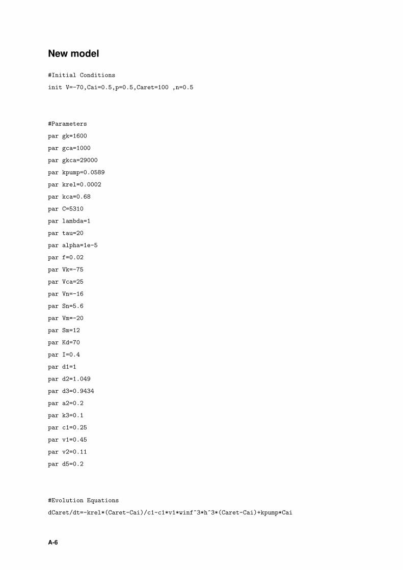
New model
#Initial Conditions
init V=-70,Cai=0.5,p=0.5,Caret=100 ,n=0.5
#Parameters
par gk=1600
par gca=1000
par gkca=29000
par kpump=0.0589
par krel=0.0002
par kca=0.68
par C=5310
par lambda=1
par tau=20
par alpha=1e-5
par f=0.02
par Vk=-75
par Vca=25
par Vn=-16
par Sn=5.6
par Vm=-20
par Sm=12
par Kd=70
par I=0.4
par d1=1
par d2=1.049
par d3=0.9434
par a2=0.2
par k3=0.1
par c1=0.25
par v1=0.45
par v2=0.11
par d5=0.2
#Evolution Equations
dCaret/dt=-krel*(Caret-Cai)/c1-c1*v1*winf^3*h^3*(Caret-Cai)+kpump*Cai
A-6

dV/dt=(-Ik-Ica-Ikca)/C
dn/dt=lambda*(ninf-n)/tau
dCai/dt=f*(-alpha*Ica-kca*Cai)+krel*(Caret-Cai)+c1*v1*winf^3*h^3*(Caret-Cai)-c1*kpump*Cai
dp/dt=(pinf-p)/taup
#Currents
Ik=gk*n*(V-Vk)
Ica=gca*minf*(V-Vca)
Ikca=gkca*Cai*(V-Vk)/(Kd+Cai)
#Other functions
minf=1/(1+exp((-20-V)/12))
ninf=1/(1+exp((-16-V)/5.6))
q2=((I+d1)/(I+d3))*d2
winf=(I/(I+d1))*(Cai/(Cai+d5))
taup=1/(a2*(q2+Cai))
pinf=q2/(q2+Cai)
@ total=60000, bound=100000000
done
A-7

A-8