Modeling the Competition for Land: Methods and Application to Climate Policy*

by

Ronald D. Sands1

Man-Keun Kim2

GTAP Working Paper No. 45 2008

1Joint Global Change Research Institute, Pacific Northwest National Laboratory, 8400 Baltimore Ave., Suite 201, College Park, Maryland, 20740, USA Contact: Ronald.Sands@pnl.gov

2Department of Resource Economics, University of Nevada/Mail Stop 204, 1664 N. Virginia Street, Reno, Nevada 89557, USA *Chapter 7 of the forthcoming book Economic Analysis of Land Use in Global Climate Change Policy, edited by Thomas W. Hertel, Steven Rose, and Richard S.J. Tol

2

MODELING THE COMPETITION FOR LAND: METHODS AND APPLICATION TO CLIMATE POLICY

Ronald D. Sands and Man-Keun Kim

Abstract The Agriculture and Land Use (AgLU) model was developed at Pacific Northwest National Laboratory to assess the impact of a changed climate or a climate policy on land use, carbon emissions from land use change, production of field crops, and production of biofuels. The level of analysis to date is relatively aggregate, at the global or national scale, but the model captures important interactions such as endogenous land use change in response to a climate policy and international trade in agricultural and forest products. This paper describes exploratory efforts to extend the conceptual framework, including geographical disaggregation of land within the United States, improving the dynamics of the forestry sector, valuing carbon in forests, and land requirements for biofuel crops. Conceptual development is done within a single-country, steady-state version of AgLU. Land use is simulated with carbon prices from zero to $200 per t-C, with forests, biofuels, and food crops competing simultaneously for land.

3

Table of Contents 1. Introduction ..................................................................................................................4 2. Model Classification .....................................................................................................6 3. Model Background .......................................................................................................8 4. Model Calibration .......................................................................................................15 5. Geographical Disaggregation of Forests ....................................................................16 6. Forest Dynamics .........................................................................................................21 7. Mitigation and Forests ................................................................................................22

8. Biofuel Pathways ........................................................................................................26

9. Application .................................................................................................................27

10. Conclusions ................................................................................................................32

11. References ..................................................................................................................33

Table 1. Characteristics of selected models used for analysis of climate policy .....7 Table 2. Random variables and distribution functions ...........................................13 Table 3. Regional Mapping from GTAP to HUA ..................................................18 Table 4. GTAP Dataset Timber Definitions and Yield Function Parameters ........19 Figure 1. Allocation of land .....................................................................................10 Figure 2. Log-Gumbel probability density functions with a fixed scale parameter and varying shape parameters .................................................14

Figure 3. Gumbel probability density functions representing log of profit rates ....15 Figure 4. Major Watersheds in the United States ....................................................17 Figure 5. Tree yield growth curves for southeastern pine plantations .....................20 Figure 6. Tree yield growth curves for the Pacific Northwest .................................20 Figure 7. Levelized net present value per hectare for southern pine plantation trees ..........................................................................................................25 Figure 8. Levelized net present value per hectare for Pacific Northwest plantation trees .........................................................................................25 Figure 9. Land area for coarse grains in the base year.............................................28 Figure 10. Optimal tree harvest age as a function of the carbon price ......................29 Figure 11. United States land use for scenarios at various carbon prices .................30 Figure 12. Simulated land use in the United States as a function of carbon price ....31

4

MODELING THE COMPETITION FOR LAND: METHODS AND APPLICATION TO CLIMATE POLICY

Ronald D. Sands and Man-Keun Kim 1. Introduction Energy-economy models used for analysis of climate policy are under continuous development to expand the range of options for reducing net emissions of greenhouse gases. The classes of mitigation options under consideration include improvements in energy efficiency, switching to less carbon-intensive fuels, carbon dioxide capture and storage, reductions in emissions of non-CO2 greenhouse gases, and terrestrial mitigation options. The terrestrial options can be further broken down into afforestation, changes in forest management, production of biofuels, and enhancement of soil carbon. Therefore, we are moving toward top-down models with agriculture-energy-economy capabilities. Adding a capability for terrestrial mitigation options to existing energy-economy models presents challenges in both conceptual development and data requirements. One of the biggest conceptual challenges is determining a practical economic structure to simulate the competition for land, a heterogeneous natural resource. Several approaches have been demonstrated, including mathematical programming (Adams et al., 1996), partitioning land into relatively homogeneous agro-ecological zones (Darwin et al., 1995), and our approach of defining a joint probability distribution of land productivity across various land uses. A second major challenge is determining the characteristics of forests that should be retained in top-down economic models used for analysis of climate policy. Several complex forestry models are in use (e.g., Sedjo, 1990) and they provide guidance for determining the set of forest characteristics that are essential to understanding behavior under a climate policy. For example, a value on carbon provides an incentive for forest managers to increase the time between planting and harvest. Sohngen and Brown (2006) explore the cost of sequestering carbon by extending tree rotation ages. This suggests that the harvest age of trees could be an endogenous variable in agriculture-energy-economy models. A third challenge is finding a way to value carbon in all of the various land uses. If carbon is valued in some land uses, but not others, land use can shift in ways that increase carbon emissions. For example, if biofuel crops expand into land that was previously unmanaged forest, carbon stocks from the unmanaged land can be released to the atmosphere. The Agriculture and Land Use (AgLU) model was developed at Pacific Northwest National Laboratory to simulate global land use change and the resulting carbon emissions in response to a carbon policy. Edmonds et al. (1996) constructed the first version of the AgLU model as an addition to the Edmonds-Reilly-Barns (ERB) model of energy consumption and carbon emissions. ERB contains world markets for oil, gas, coal, and commercial biomass (Edmonds and Reilly, 1985). A detailed theoretical description of AgLU is provided in Sands and Leimbach (2003); we call this version AgLU 1. The

5

single composite crop in AgLU 1 was later split into four crop types for a study of US climate impacts (Sands and Edmonds, 2005) and we call this version AgLU 2. Other global models of agriculture and land use include IMAGE (Alcamo et al., 1998), FARM (Darwin et al., 1995), and the IIASA Basic Linked System (Fischer et al., 1988). These models are similar on the demand side: consumer preferences and income influence demand for agricultural products. However, the supply side of IMAGE stands in contrast to the other models with its grid-cell level of land-use detail and set of allocation rules for land. FARM and the Basic Linked System use market-clearing prices to allocate land resources among competing uses, but do not match land use to specific geographic locations. The Forestry and Agricultural Sector Optimization Model (FASOM) allows for land transfers between forestry and agriculture, recognizing that forestry decisions are inherently dynamic, spanning several decades (Adams et al., 1996). The land allocation methodology used here is adapted from Clarke and Edmonds (1993), which considers the related problem of selecting a set of energy technologies to produce a given energy service at minimum cost. Instead, we allocate land across agricultural activities to maximize economic returns to land owners. The spatially independent approach used here is quite different than the geographically detailed approach of the IMAGE model. The three primary drivers of land use change are population growth, income growth, and autonomous increases in future crop yields. Even small changes in the rate of increase in future yields can have a large impact on the amount of cropland needed to maintain diets. Changes in the regional composition of consumption in response to higher incomes can also be important, especially if people in developing countries increase per-capita consumption of animal products to the level seen today in the United States and Europe. This paper reports on exploratory efforts to improve the methodology of AgLU in three areas: (1) geographical disaggregation of land areas in the United States, (2) improvement in forestry dynamics; and (3) the response of biofuels to a carbon incentive. Because of the complexity of forests, especially keeping track of stocks of trees by vintage and the separation in time between planting and harvest, we focus on one country (the United States) and limit our analysis to steady-state comparisons. This is not the same as a static model: the steady-state dynamics are consistent with an intertemporal model that has reached steady-state. We call this exploratory version AgLU 2x. We first construct a steady-state base-year scenario for the United States with 18 subregions, calibrated to agricultural and forestry production in 1990. Then we apply a carbon price ranging from zero to $200 per metric ton of carbon (t-C), and allow the managed forestry sector to endogenously select the optimal tree rotation at each carbon price. We run this experiment once more with an incentive for biofuels, using a stylized cellulosic conversion process of switchgrass to ethanol. The paper is organized as follows. Section 2 describes the relationship between AgLU and specialized forestry models. Section 3 provides a summary of the land allocation methodology and Section 4 covers base-year calibration. The next three sections

6

describe extensions on geographical disaggregation, forest dynamics and how the forest dynamics change with a carbon price. Section 8 describes biofuel pathways and Section 9 provides sample model output. A final section provides our conclusions and areas for further research. 2. Model Classification Forests are an important part of land use because they occupy a large area of land and standing forests contain a large amount of carbon. Economic simulation of land use, especially land use decisions related to climate policy, should therefore include forestry as an option. However, forestry is inherently intertemporal because of the time lag between planting and harvesting, and this presents a challenge to include forestry in models that do not have a capability for intertemporal optimization. Early attempts to include forestry in AgLU, without acknowledging the intertemporal nature of forest decisions, were not successful. They led to unstable simulations of land use over time with under planting and over planting of forests. This problem was solved by creating a forward market for forest products, which is the intersection of a supply curve based on present planting and a demand curve for forest products at the time of harvest. AgLU is static outside of forestry and the intertemporal capability for forest products was possible only with the simplifying assumption that the harvest age for trees is exogenous and fixed. Specialized forestry models handle forest dynamics directly within an intertemporal optimization framework. They generally maximize the discounted sum of producer and consumer surplus. Planting and harvesting decisions are made optimally, given an initial stock of trees distributed across vintages. The transition between an initial stock of trees by vintage to an ending stock can be very complicated. However, if the driving variables, such as the demand function for forest products, are in steady state, the forest planting and harvesting decision also reaches a steady state regardless of the initial stock of trees, and the steady state equilibrium can be solved algebraically outside of the optimization model.1 Table 1 attempts to sort out key characteristics of selected models or model types relevant to the land allocation problem. We let AgLU 2 represent the version of PNNL’s Agriculture and Land Use model used in Sands and Edmonds (2005). We let AgLU 2x represent a single-country, steady-state version of AgLU that is intended to provide guidance for modeling forestry in computable general equilibrium models.

1 Sohngen et al. (this volume, Chapter 11; GTAP Working Paper No. 49) discuss the difficulty of simulating the transition of forest vintages in a computable-general-equilibrium model.

7

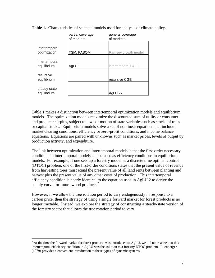
Table 1. Characteristics of selected models used for analysis of climate policy. partial coverage general coverageof markets of markets

intertemporal optimization TSM, FASOM Ramsey growth model

intertemporal equilibrium AgLU 2 intertemporal CGE

recursive equilibrium recursive CGE

steady-state equilibrium AgLU 2x

Table 1 makes a distinction between intertemporal optimization models and equilibrium models. The optimization models maximize the discounted sum of utility or consumer and producer surplus, subject to laws of motion of state variables such as stocks of trees or capital stocks. Equilibrium models solve a set of nonlinear equations that include market clearing conditions, efficiency or zero-profit conditions, and income balance equations. Equations are paired with unknowns such as market prices, levels of output by production activity, and expenditure. The link between optimization and intertemporal models is that the first-order necessary conditions in intertemporal models can be used as efficiency conditions in equilibrium models. For example, if one sets up a forestry model as a discrete time optimal control (DTOC) problem, one of the first-order conditions states that the present value of revenue from harvesting trees must equal the present value of all land rents between planting and harvest plus the present value of any other costs of production. This intertemporal efficiency condition is nearly identical to the equation used in AgLU 2 to derive the supply curve for future wood products.2 However, if we allow the tree rotation period to vary endogenously in response to a carbon price, then the strategy of using a single forward market for forest products is no longer tractable. Instead, we explore the strategy of constructing a steady-state version of the forestry sector that allows the tree rotation period to vary.

2 At the time the forward market for forest products was introduced to AgLU, we did not realize that this intertemporal efficiency condition in AgLU was the solution to a forestry DTOC problem. Luenberger (1979) provides a convenient introduction to these types of dynamic systems.

8

3. Model Background This section describes the features of AgLU 2x, a steady-state equilibrium model of United States land use and agricultural production. At the core of AgLU is a mechanism to allocate land among crops, pasture, and forests according to the economic return from each land use type. A joint probability distribution is defined over yield in each alternative land use. With additional information on prices and non-land cost of production, each landowner is assumed to select the land use with the greatest economic return calculated as revenue less non-land cost of production. With simplifying assumptions on the geographic distribution of yield, a reduced-form solution can be obtained for the share of total land in each region allocated to each land use as a function of prices and non-land costs of production. See Sands and Leimbach (2003) for a more complete theoretical description of AgLU and an application to the role of biomass-based fuels in a carbon-constrained world. Agricultural data for base-year calibration at the national level are obtained from the Food and Agriculture Organization (FAO) of the United Nations. Crop yield at the subregion level in the United States is calculated by aggregating county-level agricultural data from the United States Department of Agriculture to the 18 water basins used in AgLU 2x. Calories are the basic unit of measurement in AgLU. Food consumption is measured as kilocalories per person per day, while crop yields have units of gigacalories per hectare. Much of the original FAO data used to calibrate AgLU are in units of kilograms, which are converted to calories using weights with units of calories per gram. Calories are a convenient unit of measure for consumer demand because it provides a physical link from final demand for food to demand for primary calories, through conversion efficiencies for processed food and animal products, to the demand for land, through crop yields. As indicated in Table 1, AgLU 2x includes extensions from a partial to general equilibrium framework. The major additions include a consumer demand system based on a utility function, markets for labor and capital, a large “everything else” sector to represent non-agricultural production, and configuring base-year benchmark data in the form of a social accounting matrix. One advantage of a general equilibrium framework is that diagnostics used in general equilibrium applications, such as a Walras’ Law test, can be applied to test model integrity. Placing benchmark data in a social accounting matrix will aid in future integration of AgLU 2x into a multi-sector general equilibrium model. Demand Agricultural production and land use are driven primarily by the demand for food. Consumer demand for food creates direct demands for crops as well as indirect demands through consumption of animal products and processed crops. FAO food balance data cover three broad food categories: crops consumed directly, crops consumed indirectly as processed crops, and animal products. Direct crop consumption is primarily of cereals, but also includes starchy roots, fruits and vegetables. Processed crops include vegetable

9

oils from oil crops, sweeteners from sugar crops, and alcoholic beverages. Animal products include meat, milk, butter, eggs, and animal fats. Consumer demand for all products is determined using the Linear Expenditure System (LES), which is convenient because one can specify a minimum required amount of consumption for each commodity. Per-capita consumption for each commodity in each region is given by

⎟⎠

⎞⎜⎝

⎛−+= ∑

kijijj

i

iijjij xpm

pxmpx β),( (3.1)

where i is a commodity index, j is a region index, x is quantity demanded per capita, p is a price vector, m is income per capita, x is a minimum quantity of consumption, and β is a share parameter. Units of food consumption are calories per person and the minimum quantity is expressed in the same units. Consumption of forest products is measured in cubic meters. The i index covers the following commodities: rice, wheat, coarse grains, oil crops, sugar crops, other food crops, nonfood crops, processed crops, chicken and pork, beef, forest products, and everything else. Demand for agricultural products varies with population and through the price and income elasticities. Care must be taken in setting demand function parameters so that simulated consumption stays within a plausible range in each region and food commodity. Demand for processed crops creates an indirect demand for crop land through the conversion of crops to vegetable oils, sweeteners, and alcoholic beverages. Demand for animal products creates an indirect demand for crop land and pasture land used as animal feed, but with a net loss of calories through the conversion from crops to animal products. Demand for biomass fuels also requires crop land, especially in scenarios with high prices of fossil fuels, or scenarios that place a high value on limiting carbon dioxide emissions. Prices of agricultural products adjust to equate supply and demand, where supply is determined by a land allocation mechanism and assumptions on yield. Supply Supply of crops, biomass, pasture, and forest products is calculated as the amount of land allocated to each land use times average yield. Animal products are produced with a combination of crop-based feed and pasture. A tree diagram (Figure 1) shows how land is allocated among alternative uses. Land is allocated among food and biomass crops, pasture, and trees. Crops and commercial biomass are grouped in a separate nest because we assume land for growing commercial biomass competes directly with land for growing crops.

10

cropland

biomasscrops

managed forest grasslandunmanaged

hayoil nonfoodcrops

wheat rice coarsecropsgrains

other foodsugarcrops crops

Figure 1. Allocation of land. Selection of land use is based on maximizing economic return per hectare, calculated as revenue less production cost, at each location. Profit per hectare is equal to revenue (yield per hectare times price received) less production cost (yield per hectare times non-land cost per unit of output). An average profit rate, in dollars per hectare, is calculated for each land use as ( )iiii gpy −=π i = land uses requiring cropland (3.2) where iy is the intrinsic yield for land use i, pi is the price received for the product produced by land use i, and gi is the non-land cost per unit of output in land use i. Intrinsic yield is an average yield across all possible locations where a crop could be grown, regardless of the actual land use selected by profit-maximizing land owners. The yield distribution within a region implicitly represents variation across temperature, precipitation, available sunlight, soil quality, and topography. Between regions, the yield distribution also captures differences in technology and management practice. Given a joint probability distribution of yield, information on prices received, and non-land costs of production, it is possible to calculate the share of land allocated to each use and the average yield within each land use. With specific assumptions on the functional form of the yield distribution, the share of cropland allocated to use i is given by

∑

=

kk

iis

2

2

1

1

λ

λ

ππ (3.3)

Where 21 λ is a positive parameter (an elasticity) that determines the rate that land shares change in response to changes in profit rates. The subscript on lambda refers to the lower nest for land uses requiring cropland. This equation has the desirable properties that

11

greater profit rates imply greater shares of land; it can be calculated quickly; and the shares sum to one.3 An observed average profit rate for all land within crops is written as a function of the individual profit rates. This is shown in Equation (3.4) where k is an index across cropland use types. The average profit rate for all cropland is greater than any of the individual profit rates.

2

21λ

λππ ⎥⎦

⎤⎢⎣

⎡= ∑

kkcropland (3.4)

The share of land allocated to forests depends on the profit rate for trees, which depends on the price received for forest products harvested in the future. This future price is determined by equating supply and demand in a market for forest products at the time of harvest. The profit rate calculation for land allocated to forest products is analogous to equation (3.2) and is given by

( )

( )forestforestforestAforest gpyrr

−−+

= ~11

π (3.5)

where r is the interest rate and forestp~ is the price per cubic meter of forest products and A is the tree lifetime. In previous versions of AgLU, the tree lifetime was set exogenously. In this paper we allow A to respond optimally to changes in the prices of forest products and a carbon price. Grassland provides a challenge for a modeler as much of it is too dry for crops but it is useful for grazing livestock. In this study, we have assumed it is useful only for grazing and is not part of the land allocation decision.4 The remaining land type is unmanaged land, which is primarily unmanaged forest. Even though the land is unmanaged in terms of commodities, it is assumed to provide environmental services. During model operation, the profit rate for unmanaged land is fixed, and all other profit rates are relative the profit rate for unmanaged land. An average profit rate across all possible land uses is given by [ ] 1111 111ˆ λλλλ ππππ unmanagedforestcropland ++= (3.6)

3 There are several similarities between the land supply structure used here and the constant elasticity of transformation (CET) approach used in Hertel at al. (this volume, Chapter 6; GTAP Working Paper No. 44). Both approaches allow greater substitutability between crop types than between larger aggregates of land. Further, Hertel et al. (this volume, Chapter 1; GTAP Working Paper No. 39) note that there is a direct mapping from parameters of the AgLU land supply structure to the transformation parameter in the CET function. The substitution elasticity used here for crop types ( 21 λ ) is directly comparable to the absolute value of the CET transformation parameter omega in Chapter 6 of this volume; GTAP Working Paper No.44. 4 Grassland might also be unsuitable for crops because of slope, distance from roads, or poor soils.

12

Since all land uses are included, π is the observed average profit rate in dollars per hectare of land. An interesting result is that observed average profit rates are equal across all land use types. In other words, the average profit rate across land in wheat is the same as the average profit rate across land in managed forests. This result is not derived here, but is a consequence of economic optimization. ππ ˆˆ =i i = all land uses (3.7) We exploit this result to calculate an observed average yield for each land use analogous to Equation (3.2). The observed average yield for any land use (except forestry) is given by

ii

i gpy

−=

πˆ i = all land uses except forestry (3.8)

Therefore, the observed average yield is defined to be the yield at which the profit rate is equal to iπ . Average yield is multiplied by the amount of land, given by the land share equation to determine supply. The average yield for managed forests includes a discount factor and is given by

rr

gpy

A

forestryforestryforestry

1)1(~

ˆˆ −+−

=π (3.9)

An important feature of this land allocation mechanism is that, for any given land use, average yield may fall as the amount of land allocated to that use increases. For example, if the most productive land is first allocated to crops, cropland can only expand into land less suitable for crops. Statistics of Land Allocation Sands and Leimbach (2003) provide a fairly complete mathematical description of the land allocation methodology in AgLU. This section provides a simplified graphical description of the methodology. The lambda parameter in Equation (3.3) is a function of the underlying crop yield distribution and the correlation coefficient between land uses. r−= 1σλ (3.10) where r is the correlation coefficient between land uses and σ is the shape parameter of a Log-Gumbel distribution function for crop yield. The AgLU land allocation mechanism considers crop yield a random variable, which implies that the rate of return to land (profit rate) is also a random variable.

13

( )iiikik gpy −=π i = land use; k=location (3.11) At any location k within a land area, the land owner selects land use i with the greatest profit rate. If the profit rate is distributed Gumbel for each land use, with a constant variance (or scale parameter) across land uses, then a closed-form land share equation exists. However, the variance of the profit rate will change along with prices, so we cannot use profit rate directly in land allocation. Instead, we maximize the log of profit rate at each location. )ln()ln()ln( iiikik gpy −+=π i = land use; k=location (3.12) Now the price term is simply a translation parameter and does not affect the variance of the distribution of log of profit rate. Table 2 summarizes the parameters for distributions of the log of profit rate, profit rate, and yield. We start by requiring that the log of profit rate be distributed Gumbel to ensure that a closed-form land share equation exists. If the log of profit rate is distributed Gumbel, then the profit rate must be distributed Log-Gumbel, and therefore yield is distributed Log-Gumbel. Table 2. Random variables and distribution functions

parameters variable distribution location scale shape yield Log-Gumbel (none) iy σ profit rate Log-Gumbel (none) iπ σ ln(profit rate) Gumbel ( )iπln σ (none) The variance parameter σ in the Gumble distribution becomes a shape parameter in the Log-Gumbel distribution. Figure 2 provides the probability density function for the Log-Gumbel distribution with various shape parameters. See Bury (1999) for background on the Gumbel and other distributions. If this distribution function represents crop yields, then a value for σ less than one provides a better match to historical crop yields than other values for σ. One drawback of this distribution function is the thick upper tails which imply some probability of unrealistically high crop yields.

14

σ = 2

σ = 1

σ = 0.5

σ = 0.3

σ = 0.2

0

0.1

0.2

0 10 20 30 40

Figure 2. Log-Gumbel probability density functions with a fixed scale parameter and varying shape parameters. Figure 3 provides a stylized example of the use of Gumbel distribution functions to determine the distribution of profit rates resulting from land competition. Let land use A have a lower average (log) profit rate across locations than land use B. Some locations will yield greater returns to land use A and some locations to land use B. The Gumbel distribution furthest to the right in Figure 3 is the distribution of log profit rates after competition. In this example, land use A occupies 36% of the land and land use B occupies 64% of the land.

15

0.0

0.1

0.2

0.3

0.4

0.5

0.6

0.7

0.8

0.9

1.0

0 1 2 3 4 5 6

Land Use Aμ = ln(6)

Land Use Bμ = ln(8)

Optimal Mix of Land Usesμ = ln(10)

Figure 3. Gumbel probability density functions representing log of profit rates (σ = 0.5) 4. Model Calibration Before we can simulate land use, we need to determine a set of parameters: the intrinsic yield for each crop, parameters of the forest growth curve, prices consistent with general equilibrium, production function parameters, and parameters of the consumer demand system. Some parameters can be calculated directly, but others are the solution of a system of nonlinear equations. Intrinsic yield For any given crop and land area, the intrinsic yield is the average yield that would be observed if all land in that area were planted in just that one crop. In that case, the observed yield and intrinsic yield would be the same. However, crops are generally grown at locations within a land area where yield is greater than average. Therefore, intrinsic yield is less than or equal to observed average yield. Equations from Section 3 can be manipulated to show that 12ˆ λλ

icroplandii ssyy = (4.1)

16

Where scropland is the share of cropland in total land, si is the share of land use i in cropland, and iy is the observed average yield for land use i. We actually use the intrinsic yield iy as a calibration parameter to match historical data on land use. Everything on the right side of equation (4.1) can be observed from data except 1λ and

2λ . The lambda parameters are a function of the yield distribution shape parameter and the correlation between yields of different crops. Equation (4.1) provides exact land use calibration if a region is modeled without subregions, but only an approximate land use calibration for subregions within a region. Since the land shares are always less than 1, Equation (4.1) ensures that intrinsic yield iy is always less than average yield iy . For the scenarios demonstrated in this paper, we set 5.01 =λ and 35.02 =λ , which corresponds to 5.0=σ in both the top and bottom land use nests, and correlation coefficient r equal to zero in the top nest and 0.51 in the lower nest. These parameters are set more by modeler’s judgment than an empirical estimation, but the potential remains for historical data on crop yields to inform these parameters. The smaller the values of λ , the closer iy is to the historical average yield iy . Forest growth curve The forest growth curve in has three parameters; we fix one of them in advance leaving two parameters free. These free parameters are set so that we match observed yield and that the observed yield and harvest age are optimal given the interest rate and timber price. Equilibrium prices Another part of the calibration process is to find a set of prices that equate supply and demand for each commodity. These prices are needed during calibration to calculate technical coefficients of production functions and consumer demand functions. Production processes that don’t use land directly are modeled as constant-elasticity-of-substitution (CES) functions, and the Linear Expenditure System is used for consumer demand. 5. Geographical Disaggregation of Forests Previous analysis using AgLU considered a country as the smallest geographical unit. Each agricultural product, including timber, was represented across an entire country as a single average production function. This allowed us to provide global coverage and simulate global markets, but the level of geographical detail was not well suited to studies of individual countries. For example, forests in the Pacific Northwest of the United States are quite different from forests in the southeast. We are exploring an asymmetric modeling strategy that allows greater geographical disaggregation in a country of interest or where data are available, yet still links, through

17

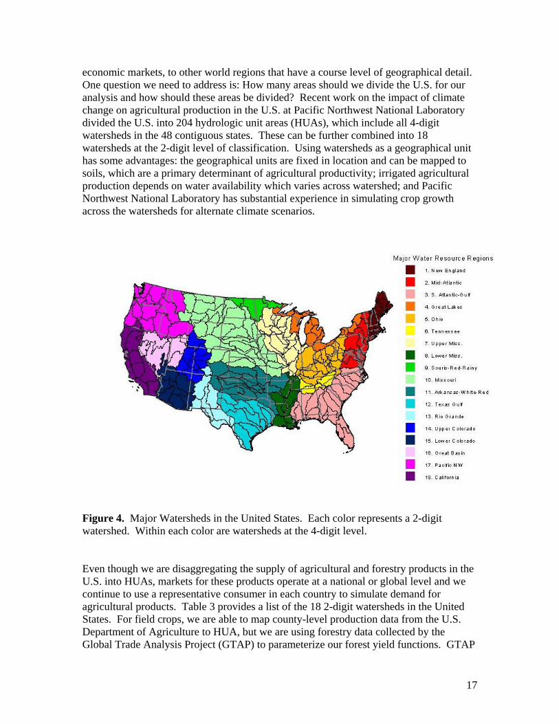
economic markets, to other world regions that have a course level of geographical detail. One question we need to address is: How many areas should we divide the U.S. for our analysis and how should these areas be divided? Recent work on the impact of climate change on agricultural production in the U.S. at Pacific Northwest National Laboratory divided the U.S. into 204 hydrologic unit areas (HUAs), which include all 4-digit watersheds in the 48 contiguous states. These can be further combined into 18 watersheds at the 2-digit level of classification. Using watersheds as a geographical unit has some advantages: the geographical units are fixed in location and can be mapped to soils, which are a primary determinant of agricultural productivity; irrigated agricultural production depends on water availability which varies across watershed; and Pacific Northwest National Laboratory has substantial experience in simulating crop growth across the watersheds for alternate climate scenarios.

Figure 4. Major Watersheds in the United States. Each color represents a 2-digit watershed. Within each color are watersheds at the 4-digit level. Even though we are disaggregating the supply of agricultural and forestry products in the U.S. into HUAs, markets for these products operate at a national or global level and we continue to use a representative consumer in each country to simulate demand for agricultural products. Table 3 provides a list of the 18 2-digit watersheds in the United States. For field crops, we are able to map county-level production data from the U.S. Department of Agriculture to HUA, but we are using forestry data collected by the Global Trade Analysis Project (GTAP) to parameterize our forest yield functions. GTAP

18

forestry data for the United States provide seven different yield functions and Table 3 shows how we map the GTAP yield functions to the major watersheds in the United States. Table 3. Regional Mapping from GTAP to HUA

HUA region GTAP timber type

GTAP yield

function

Cut-off agea

(years)

Observed yieldb

(m3/ha) New England M4, M10 4 70 114 Mid Atlantic M4, M10 4 70 114 S-Atlantic-Gulf M2 2 30 280 Great Lakes M4, M10 4 70 114 Ohio M11, M13 7 70 151 Tennessee M3, M9, M12 3 50 115 Up Mississippi M11, M13 7 70 151 Low Mississippi M3, M9, M12 3 50 115 Souris Red Rainy M4, M10 4 70 115 Missouri M11, M13 7 70 151 Arkansas W-R M11, M13 7 70 151 Texas Gulf M3, M9, M12 3 50 115 Rio Grande M5 5 80 151 Up Colorado M6, M7, M14 6 100 91 Low Colorado M5 5 80 151 Great Basin M6, M7, M14 6 100 91 Pacific Northwest M1 1 60 420 California M11, M13 7 70 151

a: cut-off age = total forest area / harvested area b: observed yield = production / harvested area GTAP Dataset Timber Definition and Timber Yield Function The GTAP data set provides 14 timber definitions for the United States, M1 through M14, based on regions and timber types. Each timber definition has specific yield function which is given by equation (5.1).

⎥⎦

⎤⎢⎣

⎡−

−=)(

exp)(Cage

BAagey for age > C, y(age) = 0 for age < C (5.1)

where age is timber age and A, B, and C are positive yield parameters. Timber yield has units of m3 per hectare of roundwood. The timber yield function that we actually use has enough flexibility to provide a good approximation to the GTAP functional form in Equation (5.1).

19

Table 4 provides the parameters for each GTAP forest yield function in the United States. These parameters can be substituted directly into Equation (5.1). Table 4. GTAP Dataset Timber Definitions and Yield Function Parameters

1 2 3 4 5 6 7

parameter M1, M8 M2 M3, M9,

M12 M4, M10 M5 M6,

M14, M7 M11, M13

A 9.05 6.68 6.455 8.2 8.5 8.5 7.92B 141.63 25 25 141.63 165 159.51 110C 10 10 30 20 20 20 20

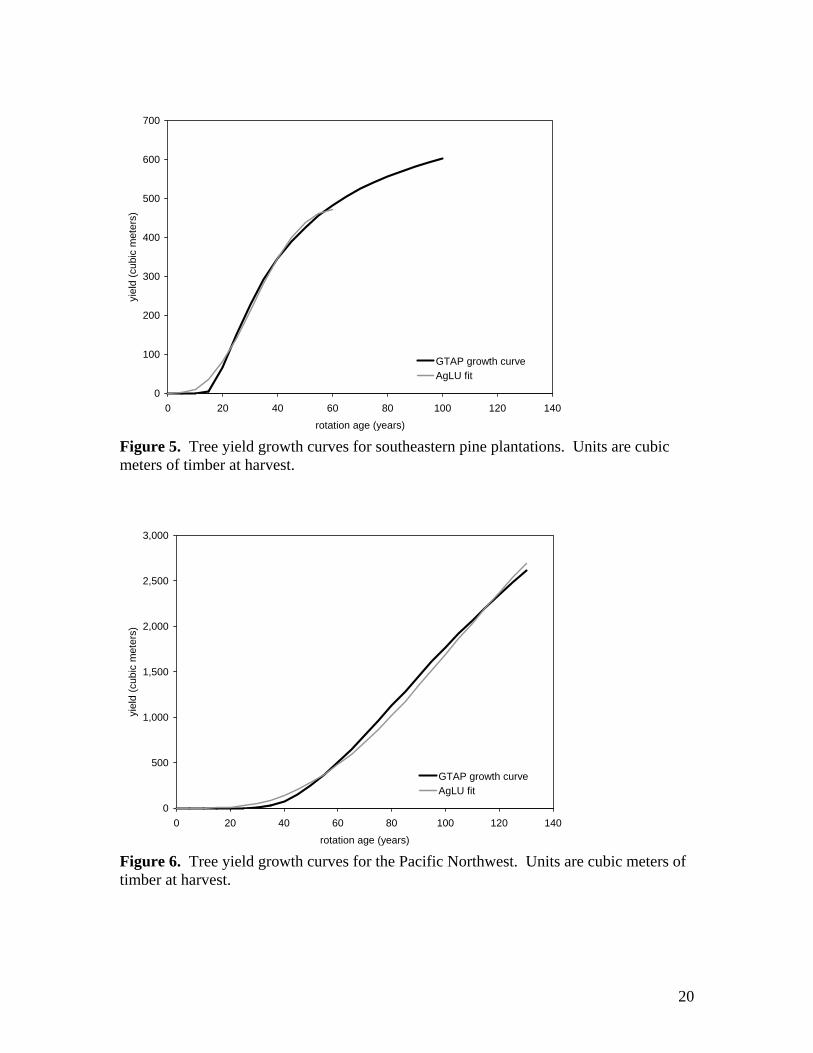
M1 = Pacific Northwestern west side M2 = Southern pine plantation M3 = Southern softwood M4 = Northern softwood M5 = Interior/Mountain softwood M6 = Low access northern softwood M7 = Low access interior softwood M8 = Low access Pacific Northwestern softwood M9 = Southern hardwood M10 = Northern hardwood M11 = Temperate hardwood M12 = Southern mixed forest M13 = Temperate mixed forest M14 = Low access northern mixed forest We use a different functional form than GTAP and construct an approximation with a least-squares fitting procedure. Figures 5 and 6 show this fit for the southeastern pine plantation and Pacific Northwest. We use Equation (6.1) so that all calculations of net present value at various carbon prices are available in a closed form. However, the least-squares fit with this functional form is not good at high rotation ages, and we must check that model output stays within a range where we have a good fit to the growth curve. Sohngen et al. (this volume, Chapter 35) note that the GTAP growth curves are only valid over the range of rotation ages where historical data are available. Therefore, further work is needed to parameterize growth curves for higher rotation ages, especially if we wish to simulate the response to carbon prices above $200 per t-C.

5 GTAP Working Paper No. 41

20

0

100

200

300

400

500

600

700

0 20 40 60 80 100 120 140rotation age (years)

yiel

d (c

ubic

met

ers)

GTAP growth curveAgLU fit

Figure 5. Tree yield growth curves for southeastern pine plantations. Units are cubic meters of timber at harvest.

0

500

1,000

1,500

2,000

2,500

3,000

0 20 40 60 80 100 120 140rotation age (years)

yiel

d (c

ubic

met

ers)

GTAP growth curveAgLU fit

Figure 6. Tree yield growth curves for the Pacific Northwest. Units are cubic meters of timber at harvest.

21

6. Forest Dynamics In this section, we derive the conditions for determining the optimal tree rotation age, known as the Faustmann equation. The optimal timber rotation is a function of the interest rate, the price received for forest products, harvesting cost, regeneration cost, and the shape of the tree growth curve. We provide several interpretations of the Faustmann equation at the end of this section. Timber Growth Function We select a functional form for the timber yield function from van Kooten et al. (1995) that is flexible enough to describe timber growth over time, yet can be modified to account for carbon sequestration incentives paid to owners of forested land. The timber yield function is )exp()( 31

2 acacay c −= (6.1) where c1, c2 and c3 are associated parameters and a is timber age. If c2 is an integer, in this case c2 equals 4, the yield function has a closed-form integral over the timber age.6 This property of the yield function becomes useful when considering carbon incentives. We use GTAP database to calibrate parameters, which is available at http://www-agecon.ag.ohio-state.edu/people/sohngen.1/forests/GTM/. Sohngen and Tennity (2004) describes a dataset which is containing inventory and economic information on global forests such as timber inventory by vintage, timber production, prices, costs, yield function parameters and carbon contents. Determination of Optimal Timber Rotation We derive the efficiency condition that determines the optimal timber rotation based on maximizing net present value, also know as the Faustmann equation. Consider the problem of a forest land owner to determine the optimal age of trees at harvest. The net present value (NPV1) of timber per hectare for a single forest rotation is calculated as follows: [ ] g

raht cecaypaNPV −−= −)()(1 (6.2)

6 First derivative is given by )()exp()( 33

)1(21

2 aycacaccay c −−=′ − ; the integration over rotation is

given by ∫ ⎟⎟⎠

⎞⎜⎜⎝

⎛+−−−−−=

−−−−−a Tcacacacac

cce

caec

cea

cea

ceacay

0 53

53

53

333

2

23

3

3

4

1242424124)(

33333

A direct calculation of this integral is useful for calculating the optimal rotation age with a carbon incentive. The CRC Standard Mathematical Tables (Beyer, 1978) is a useful reference to determine which types of exponential functions have a closed-form integral.

22

where a is the timber age, )(ay is the timber yield function, tp is timber price, hc is harvesting cost, gc is regeneration or planting cost and r is the interest rate. This is the same functional form as in van Kooten et al. (1995), except here we include cg. Based on equation (6.3) we can calculate the NPV of timber benefits over all future rotations:

raeaNPVaNPV −−

=1

)()( 1 (6.3)

The optimal timber rotation a* maximizes NPV, which is found by differentiating NPV with respect to a, setting the derivative equal to zero and rearranging;

( ) **

*

1*)(*)(

rag

raht

gra

t

er

cecayprceayp

−−

−

−=

−−−′

(6.4)

Equation (5.4) collapses to that in van Kooten et al. if cg equals zero. Equation (5.4) is not easy to interpret and there are other ways to arrange the equation for an easier interpretation. Equations (6.5) and (6.6) are mathematically equivalent but offer somewhat different interpretations.

( )ghtrat ccayperayp −−

−=′

− *)(1

*)( * (6.5)

The left hand side of Equation (6.5) is the increment to revenue from increasing tree rotation by one year; the right hand side is net revenue at harvest annualized over all years in the tree rotation. )*)((*)( *

gra

t caNPVreayp +=′ − (6.6) The left hand side of Equation (6.6) is the present value of the increment to revenue from increasing tree rotation by one year; the right hand side is the interest rate times NPV(a*) plus the interest rate times regeneration cost. 7. Mitigation and Forests The optimal tree rotation age turns out to be sensitive to carbon payments for carbon sequestered in forests. The greater the carbon price, the longer trees are grown until harvest. We provide numerical examples of this relationship for Pacific Northwest trees and southeastern U.S. pine plantations. Carbon prices and the Faustmann equation Here we modify the equation for the net present value across a single forest rotation to account for a carbon incentive paid to owners of forest land as additional carbon is

23

sequestered and a penalty paid by the land owner at the time of harvest. Following van Kooten et al. (1995), the net present value of the carbon sequestration over a rotation of length a is given by

∫ −′=a rx

cA dxexykpaNPV0

)()( (7.1)

where pc is the price of the carbon, k is a factor to convert cubic meters of timber to metric tons of carbon, and a is the age at harvest. Equation (7.1) can be modified to equation (7.2) using integrating by parts;

⎥⎦⎤

⎢⎣⎡ += ∫ −− a rxra

cA dxexyreaykpaNPV0

)()()( (7.2)

Equation (7.2) will be useful when we differentiate with respect to a. The net present value of timber from harvesting includes benefits from harvesting timber as well as the carbon penalty which represents the cost of the carbon released at the time of harvesting. The amount of carbon release to the atmosphere is expressed using the fraction )1( β− of timber. If β equals zero, then all of the carbon is released to the atmosphere. Thus the net present value (NPVB) from the carbon penalty at harvest is given by ra

cB eaykpaNPV −−−= )()1()( β (7.3) We can calculate the net present value over all of the future timber rotations as

raBA

eaNPVaNPVaNPV

aNPV −−++

=1

)()()()( 1 (7.4)

The optimal timber rotation age that takes into account both timber harvested and carbon benefit and a carbon penalty for releasing carbon is found by differentiating equation (7.4) with respect to a and setting the result equal to zero. Let the numerator of Equation (7.4) be f(a) and the denominator be g(a). The modified Faustmann condition is derived by differentiating with respect to a using the quotient rule and setting the derivative to zero:

)()('

)()('

agag

afaf

= , or (7.5)

ra

ra

a rxcg

rah

ract

rac

rah

raract

ere

dxexykrpceceaykpp

eakyrpercearyeaykpp−

−

−−−

−−−−

−=

+−−+

++−+

∫ 1)()()(

)())()(')((

0β

β (7.6)

Note that setting 0=cp gives a result identical to Equation (5.4).

24

Carbon incentives: rental payments on stored carbon or full carbon payment at the time of sequestration? The carbon accounting in Equations (7.1) through (7.3) provides a credit as carbon is sequestered and requires a payment as carbon is emitted. An alternative view is to provide a rental payment, based on the interest rate and carbon price, for the carbon stock each year. In this case there is no penalty for cutting trees, only a rental payment for carbon storage. If we set β from Equation (7.3) equal t zero, allowing all carbon at harvest to be emitted to the atmosphere, then we can compare the two accounting approaches directly and show they are equivalent. With β equal to zero,

∫ −=+a rx

cBA dxexykrpaNPVaNPV0

)()()( (7.7)

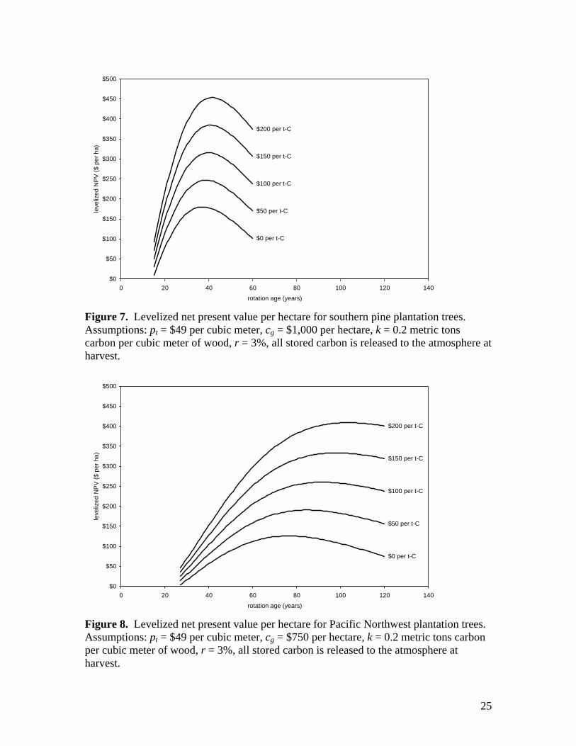
The right hand side of Equation (7.7) is the sum of rental payments for carbon stored from planting to harvest, discounted to the present. Numerical Examples Figures 7 and 8 provide numerical examples of net present value calculations for southern pine plantation and Pacific Northwest plantation trees. As was shown earlier, the growth curves for these tree types are very different from each other and the optimal tree rotation is also different. In each figure, the levelized net present value (LNPV) per hectare of land is calculated across rotation ages. The levelized net present value is the annual profit available to pay for land and is a function of the timber price, interest rate, harvest cost, regeneration cost, and carbon price. The following observations are demonstrated by Figures 7 and 8. First, if the carbon price is zero then the optimal rotation age is relatively well defined. Second, as the carbon price increases, the optimal rotation age increases and the LNPV also increases. Third, the optimal rotation age is much longer in the Pacific Northwest than for southern plantation pines. If the carbon price is high enough (relative to the price of timber) than the trees might never be harvested. However, the price of timber will respond to the carbon price to clear the timber market.

25

$0 per t-C

$50 per t-C

$100 per t-C

$150 per t-C

$200 per t-C

$0

$50

$100

$150

$200

$250

$300

$350

$400

$450

$500

0 20 40 60 80 100 120 140

rotation age (years)

leve

lized

NP

V ($

per

ha)

Figure 7. Levelized net present value per hectare for southern pine plantation trees. Assumptions: pt = $49 per cubic meter, cg = $1,000 per hectare, k = 0.2 metric tons carbon per cubic meter of wood, r = 3%, all stored carbon is released to the atmosphere at harvest.

$0 per t-C

$50 per t-C

$100 per t-C

$150 per t-C

$200 per t-C

$0

$50

$100

$150

$200

$250

$300

$350

$400

$450

$500

0 20 40 60 80 100 120 140

rotation age (years)

leve

lized

NP

V ($

per

ha)

Figure 8. Levelized net present value per hectare for Pacific Northwest plantation trees. Assumptions: pt = $49 per cubic meter, cg = $750 per hectare, k = 0.2 metric tons carbon per cubic meter of wood, r = 3%, all stored carbon is released to the atmosphere at harvest.

26

Note that these numerical examples assume the carbon price is constant over time. These results are sensitive to the rate of increase in the carbon price and this is a topic for further investigation. Our choice of functional form, Equation (6.1), is convenient because we can still obtain closed-form integrals of the equations in this section if the carbon price is increasing at an exponential rate. 8. Biofuel Pathways The land rent for producing biofuel crops will depend on many other prices and technologies including the price of fossil fuels; the carbon price, and the cost of transporting biofuels. We consider two biofuel pathways based on switchgrass as a feedstock: switchgrass to ethanol, and switchgrass burned along with coal to generate electricity. This section generalizes the discussion of biofuels found in Sands and Leimbach (2003). The parameters and equations in this section provide a way to calculate the willingness to pay for land for various biofuel pathways. Switchgrass to Ethanol We first calculate the value of ethanol as a function of the price of its substitute (gasoline) in $ per GJ, the carbon price in $ per kg-C, and the carbon content of refined petroleum (GHGoil) in kg-C per GJ. oilcarbongasolineethanol GHGPPP ×+= (8.1) Once the value of ethanol is determined, we can back out the value of switchgrass as a function of the energy content of switchgrass (EtoBio) in GJ per t of dry switchgrass, the cost of transforming switchgrass to ethanol (Ctransform) in $ per GJ, the cost of transporting switchgrass from the field to a processing plant (Etransport) in $ per GJ, and other parameters defined previously. The price of switchgrass has units of $ per t of dry biomass. The most uncertain parameter in Equation (8.2) is the cost of transforming solid biomass to liquid ethanol. ( )( )oilcarbongasolinetransporttransformethanolsswitchgras GHGPPECPEtoBioP ×+×−−×= (8.2) We could substitute Equation (8.1) into Equation (8.2) to obtain the price received for switchgrass at the farm as a function of the carbon price, the price of gasoline, emissions coefficients, and other parameters.

27

Switchgrass burned with coal to generate electricity Another pathway for switchgrass is to burn the biomass directly with coal to generate electricity, avoiding the cost of converting solid biomass to a liquid fuel. In this case, the value of switchgrass as a solid biofuel depends on the price and carbon content of coal. coalcarboncoalbiofuel GHGPPP ×+= (8.3) The price received for switchgrass at the farm (Pswitchgrass) is a function of the price of switchgrass as a biofuel at the electricity generating plant (Pbiofuel) and the cost of transporting switchgrass to the generating plant. ( )( )oilcarbongasolinetransportbiofuelsswitchgras GHGPPEPEtoBioP ×+×−×= (8.4) Land rent for producing switchgrass crop Regardless of the biofuel pathway for switchgrass, we can calculate a willingness to pay for land from the price received for switchgrass, and nonland costs of production. nonlandsswitchgrassswitchgrasland CYieldPP −×= (8.5) ( ) otheroilcarbongasolineharvestnonland CGHGPPEC +×+×= (8.6) Nonland costs of production are separated into energy and other costs in Equation (8.6). A full accounting would expand Equation (8.6) to include the cost and emissions coefficient of fertilizer. 9. Application A workbook was constructed to simulate land use in the United States with the extensions described in this paper. The workbook includes a calibration worksheet where input data is stored and initial model parameters are calculated. Model parameters are then transferred to the simulation worksheet. The simulation worksheet computes a steady-state general equilibrium of the following production sectors: the nine agricultural products in the cropland nest in Figure 1; processed crops, primarily sweeteners and cooking oil; products from cows and sheep; products from pork and poultry; forest products; and a large “everything else” sector representing the rest of the economy. Base-Year Calibration Part of the calibration process is a search for prices that equate supply and demand in all markets. If we are simulating land use for a single country and there are no land

28

subregions, then we can calibrate exactly to historical land area and yield for each land use. We use Equation (4.1) to set intrinsic yields, which along with calibration prices, allow for exact calibration to land use and average yield. Prices and intrinsic yield provide the calibration parameters to match historical land use and yield by crop type. However, we can no longer rely on base-year prices for calibration by subregion within a country; prices are the same across subregions. We could instead use nonland costs of production as a calibration parameter, but we prefer that production costs be exogenous data and not calibration parameters. It turns out that we still obtain a reasonable match to base-year data by subregion by only using Equation (4.1) to set intrinsic yields in each subregion. Figure 9 provides an example of the match to historical land use in the United States by subregion for coarse grains. This shows a concentration of production in the United States corn belt.

0.0

3.0

6.0

9.0

12.0

15.0

New

Eng

land

Mid

Atla

ntic

S-A

tlant

ic-G

ulf

Gre

at L

akes

Ohi

o

Tenn

esse

e

Up

Mis

siss

ippi

Low

Mis

siss

ippi

Sou

ris R

ed R

ainy

Mis

sour

i

Ark

ansa

s W

-R

Texa

s G

ulf

Rio

Gra

nde

Up

Col

orad

o

Low

Col

orad

o

Gre

at B

asin

PN

W

Cal

iforn

ia

milli

on h

a

Simulated Historical

Figure 9. Land area for coarse grains in the base year (1990) Sequestration of Carbon in Forests We have constructed scenarios where carbon prices increase in increments of US$ 20 up to US$ 200. These scenarios have no time dimension but instead represent the steady-state response of land use, including a change in tree rotation age, to a carbon price. Figure 10 shows how the optimal harvest age for managed forests increases with the carbon price, for trees in various United States subregions. A longer tree rotation means

29

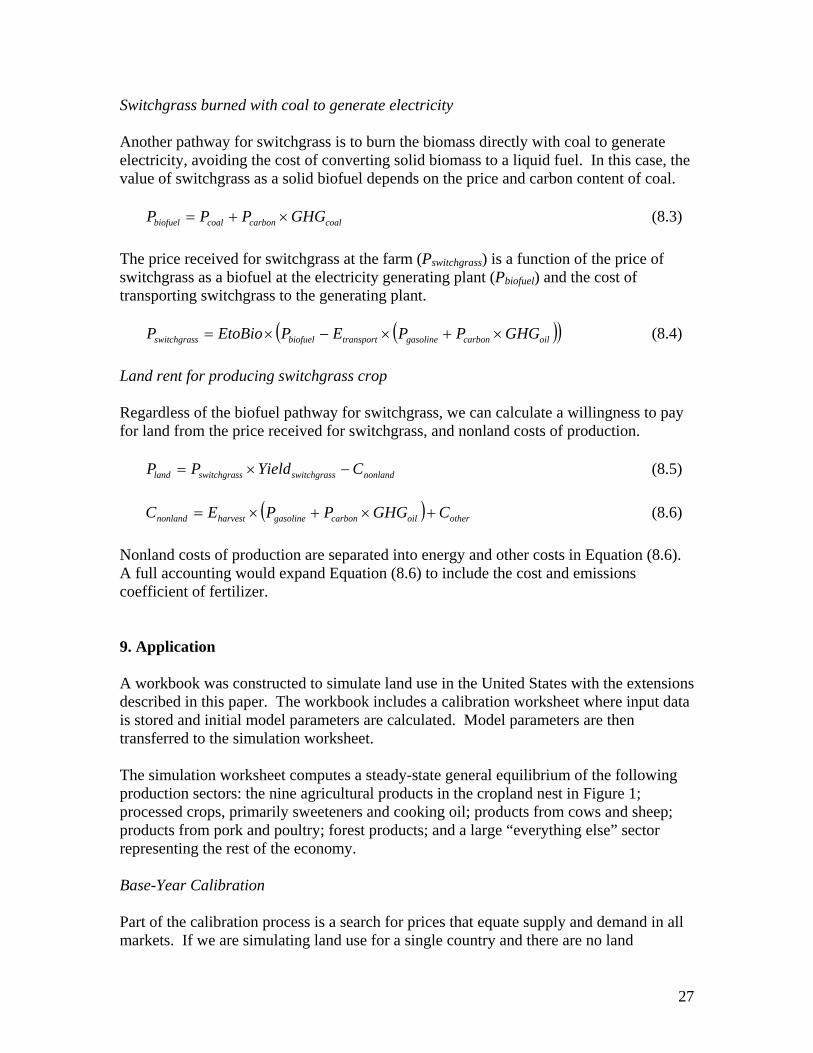
that more carbon is stored in above-ground forest biomass. Figure 11 describes land use for the same scenarios. The most interesting aspect of the land use scenarios is that land required for forests stays relatively constant up to a carbon price of US$ 100, even though the rotation age is greater. This is because the slope of the tree growth curve, at the optimal rotation age with no carbon price, is still quite steep. The increase in yield due to an extra year of tree growth more than compensates for the extra land needed to add another vintage of trees. Of course, there is a point where the increase in yield is less than the land required for another tree vintage. This point can be found by drawing a straight line from the origin of a tree growth curve to a point of tangency with the tree growth curve. After this rotation age, land required for forests increases with the carbon price. These results are sensitive to the shape of the tree growth curve, and require that we determine what the growth curves look like for harvest ages beyond 100 years.

Pacific NWPacific NW (with

biofuels)

Southeast Pines

0

20

40

60

80

100

120

140

160

0 20 40 60 80 100 120 140 160 180 200

carbon price ($ per t-C)

tree

rota

tion

(yea

rs)

Figure 10. Optimal tree harvest age as a function of the carbon price. Solid line represents scenario without biofuels. Dashed line indicates scenario with biofuels competing for land.

30

cropland

pasture and fallow

managed forest

unmanaged forest

0

50

100

150

200

250

300

350

400

450

500

0 20 40 60 80 100 120 140 160 180 200

carbon price ($ per t-C)

land

are

a (m

illion

ha)

Figure 11. United States land use for scenarios at various carbon prices. The tree rotation age is endogenous in these scenarios. Biofuels and Land Use We present here a sample land use scenario for the United States. This scenario does not have a time dimension: population and agricultural productivity are held constant. However, it is a steady-state representation of land use in the United States as a carbon price is raised to US$ 200 per metric ton of carbon in increments of US$ 20.

31

cropland

pasture and fallow

biomass

managed forest

unmanaged forest

0

50

100

150

200

250

300

350

400

450

500

0 20 40 60 80 100 120 140 160 180 200

carbon price ($ per t-C)

land

are

a (m

illion

ha)

Figure 12. Simulated land use in the United States as a function of carbon price. Population and agricultural productivity are held constant. The biofuel technology is a stylized switchgrass to ethanol process as described in Section 8. As the carbon price increases, ethanol competes directly with refined petroleum. The amount of land used for biofuels becomes quite large at higher carbon prices, with decreases in land used for pasture and unmanaged forests. Disaggregation into subregions: Does it matter? We also constructed a scenario where we considered the United States as a single land mass with a single probability distribution. The model was recalibrated so that average crop yields correspond to national average yields, tree growth curves are a weighted average of subregion growth curves, and the sigma parameters of the land allocation mechanism were increased from 0.5 to 0.8, reflecting a larger variance in the yield distribution. The results from this scenario are remarkably similar to the aggregate results from AgLU 2x with 18 subregions. Therefore, if one is interested only in aggregate national results, one can obtain a plausible scenario without splitting a region into subregions. However, there remain many reasons to construct subregions if data are available to support the disaggregation. First, we may be interested in the location of activities, such as production of biofuels. Second, we may want to construct scenarios with climate impacts, where crop yields are modified according to results from general circulation models and crop growth simulation models. These impacts are location specific. Third, we will want to add irrigated crops and water to the modeling framework, which are also location specific.

32

Finally, a single probability distribution for an entire nation cannot provide as good fit to the distribution of crop and forest yields. Using subregions allows greater flexibility for matching yield distribution functions to historical data. 10. Conclusions This study provides exploratory analysis of three model development areas: disaggregation of land in the U.S. into 18 subregions, improvements in forest dynamics, and biofuel pathways. These enhancements are not yet fully integrated into the partial and general equilibrium models used at Pacific Northwest National Laboratory for analysis of climate policy, but the methods described in this paper provide guidance as to what is feasible and practical. We divided the U.S. into 18 land subregions based on watersheds as the basis for agricultural and forest product supply. Land productivity varies across these subregions and we used forest growth curves for the Pacific Northwest and southeastern U.S. as a demonstration. There are no large conceptual difficulties to working with these subregions, but it adds to the computational burden and is data intensive. We described how managed forests respond to a carbon incentive, especially how the optimal tree rotation age increases along with a carbon incentive paid to owners of managed forests. The carbon incentive can be paid as either an annual rental payment for stored carbon or as a full payment at the time of sequestration. Our land use methodology is embedded in a simple general equilibrium framework. However, we do not attempt to capture the full dynamics of forestry that one finds in a dedicated forestry optimization model; instead, we simulate forests in their steady state. Several interesting areas remain for further investigation. First, how is the forestry analysis affected if a carbon price is increasing over time? Second, how can we best value carbon sequestered in unmanaged land? Carbon emissions from the loss of unmanaged forests are uncontrolled in our mitigation scenarios. Third, how can we include water in our analysis as a limiting factor in the supply of agricultural products? Fourth, what are the most likely biofuel pathways in each region? Finally, model enhancements are needed on the trade linkages between regions. Considerations include food security, transportation costs, and tariffs and subsidies on agricultural products.

33

References Adams, D.M., Alig, R.J., Callaway, J.M., McCarl, B.A. and Winnett, S.M. (1996) The

Forest and Agricultural Sector Model (FASOM): Model Structure and Policy Applications, Forest Service, United States Department of Agriculture, Research Paper PNW-RP-495.

Alcamo, J., Kreileman, E., Krol, M., Leemans, R., Bollen, J., van Minnen, J., Schaeffer,

M., Toet, S. and de Vries, B. (1998) ‘Global modeling of environmental change: an overview of IMAGE 2.1’, in Global Change Scenarios of the 21st Century: Results from the IMAGE 2.1 Model, Alcamo, Leemans, Kreileman (ed.), Pergamon.

Beyer, W.H. (1978) CRC Standard Mathematical Tables, West Palm Beach, Florida:

CRC Press. Bury, K. (1999) Statistical Distributions in Engineering, New York: Cambridge

University Press. Clarke, J.F. and Edmonds, J.A. (1993) ‘Modelling Energy Technologies in a Competitive

Market’, Energy Economics, 15: 123-129. Darwin, R., Tsigas, M., Lewandrowski, J. and Raneses, A. (1995) World Agriculture and

Climate Change: Economic Adaptations, Agriculture Economic Report 703, United States Department of Agriculture.

Edmonds, J.A., Wise, M.A., Sands, R.D., Brown, R.A. and Kheshgi, H. (1996)

Agriculture, Land Use, and Commercial Biomass Energy, Richland, Washington: Pacific Northwest National Laboratory, PNNL-SA-27726.

Edmonds, J.A. and Reilly, J.M. (1985) Global Energy: Assessing the Future, Oxford

University Press. Fischer, G., Frohberg, K.K., Keyzer, M.A. and Parikh, K.S. (1988) Linked National

Models: A Tool for International Food Policy Analysis, Dordrecht, Netherlands: Kluwer Academic Publishers.

Hertel, T., Rose, S. and Tol, R.S.J. (2008) ‘Land Use in Computable General Equilibrium

Models: an Overview’, Chapter 1 in Economic Analysis of Land Use in Global Climate Change Policy. Edited by T. Hertel, S. Rose, and R. Tol. Routledge

Hertel, T., Lee, H.-L., Rose, S. and Sohngen, B. (2008) ‘Modeling Land-use Related

Greenhouse Gas Sources and Sinks and their Mitigation Potential’, Chapter 6 in Economic Analysis of Land Use in Global Climate Change Policy. Edited by T. Hertel, S. Rose, and R. Tol. Routledge

34

Luenberger, D.G. (1979) Introduction to Dynamic Systems: Theory, Models, and Applications, New York: Wiley.

Sands, R.D. and Edmonds, J.A. (2005) ‘Climate Change Impacts for the Conterminous

USA: An Integrated Assessment; Part 7. Economic Analysis of Field Crops and Land Use with Climate Change’, Climatic Change, 69: 127-150.

Sands, R.D. and Leimbach, M. (2003) ‘Modeling Agriculture and Land Use in an

Integrated Assessment Framework’, Climatic Change, 56: 185-210. Sedjo, R.A. and Lyon, K.S. (1990) The Long-Term Adequacy of World Timber Supply,

Washington, D.C.: Resources for the Future. Sohngen, B., Tennity, C., Hnytka, M. and Meeusen, K. (2008) ‘Global Forestry Data for

the Economic Modeling of Land Use’, Chapter 3 in Economic Analysis of Land Use in Global Climate Change Policy. Edited by T. Hertel, S. Rose, and R. Tol. Routledge

Sohngen, B., Golub, A. and Hertel, T. (2008) ‘The Role of Forestry in Carbon

Sequestration in General Equilibrium Models’, Chapter 11 in Economic Analysis of Land Use in Global Climate Change Policy. Edited by T. Hertel, S. Rose, and R. Tol. Routledge

Sohngen, B. and Brown, S. (2006) ‘The Cost and Quantity of Carbon Sequestration by

Extending the Forest Rotation Age’, working paper available at http://aede.osu.edu/people/sohngen.1/forests/ccforest.htm

Sohngen, B. and Tennity, C. (2004) ‘Country Specific Global Forest Data Set V.1’,

memo, Dept of Agricultural, Environmental and Development Economics, The Ohio State University, Columbus, Ohio, available at http://aede.osu.edu/people/sohngen.1/forests/GTM/GTAP_datareport_v1.pdf

van Kooten, G.C., Binkley, C.S. and Delcourt, G. (1995) ‘Effect of Carbon Taxes and

Subsidies on Optimal Forest Rotation Age and Supply of Carbon Services’, American Journal of Agricultural Economics, 77: 365-374.