Modeling and Simulation of a Helicopter Slung Load Stabilization Device

Luigi S. Cicolani lcicolani@mail.arc.nasa.gov

ArmyNASA Rotorcraft Division NASA Ames Research Center, Moffett Field, CA

Maj George E. Ehlers' george.ehlers. @jsf.mil

Naval Postgraduate School, Monterey, CA

Abstract

This paper addresses the problem of simulation and stabilization of the yaw motions of a cargo container slung load. The study configuration is a UH-60 helicopter carrying a 6ft x 6 ft x 8 ft CONEX container. This load is limited to 60 KIAS in operations and flight testing indicates that it starts spinning in hover and that spin rate increases with airspeed. The simulation reproduced the load yaw motions seen in the flight data after augmenting the load model with terms representing unsteady load yaw moment effects acting to reinforce load oscillations, and augmenting the hook model to include yaw resistance at the hook. The use of a vertical fin to stabilize the load is considered. Results indicate that the CONEX airspeed can be extended to 110 kts using a 3x5 ft fin.

Introduction

The helicopter has been used since its early development for external transport of large or bulky loads to and from small austere locations, in military combat and disaster relief operations, and in civil construction, logging and fire fighting work. One limitation on these operations is that some classes of common loads, such as cargo containers, can be unstable at moderate forward speeds well below the power-limited airspeed of today's helicopters. This limits operational efficiency and hampers operations where speed or time is essential.

Military loads are certified for particular helicopter-load combinations, and these are described in the Multiservice Helicopter External Air Transport manual

'Currently at the Joint Strike Fighter Program Office, Arlington, VA

Presented at the American Helicopter Society 581h Annual Forum, Montreal, Canada, June 11-13, 2002. Copyright 0 2002 by the American Helicopter Society International, Inc. All rights reserved.

(Ref. 1). Data on the maximum acceptable airspeed from Ref. 1 are noted in Fig. 1 for various load- helicopter cases using a single point suspension. Loads with maximum speeds below 75 kts are limited well below the power limited speed of the helicopter (vH). and loads limited below 50 kts have poor stability, while loads that can be carried above 100 kts are very stable and can be flown to the helicopter limits. The load type with the largest number of cases limited by load stability is box-shaped loads (containers and vans).

Past work on load stabilization has had the objectives to (1) improve pendulum damping for precision load placement and IFR operations, (2) stabilize heading to the minimum drag orientation, and (3) extend the stable speed limits of difficult loads. Approaches to stabilization have included load ballasting, 2-point suspensions, an active arm 2-point suspension (Ref. 2): active cable winching in a 3-point suspension (Ref. 3), active reaction jets (Ref. 4), fins (Refs. 5 through 8). inertia wheels (Ref. 9), and load position or cable angle feedback (Ref. 10).

Fin stabilization of cargo containers is the subject of this paper. The fin systems attempt to stabilize the load yaw degree of freedom to achieve heading control and to extend the stable speed envelope. For cargo containers, yaw stabilization can prevent development of divergent lateral-directional motions of the load which are thought to be driven by vortex shedding as the load oscillates in yaw (Ref. 8). Previous work on fin stabilization includes a wind tunnel and flight test study of passive fins to carry bridge sections (Ref. 5) , an analytical study of two active fins mounted on a spreader bar for use with 2-point suspensions (Ref. 7), a simulation study of one or two active fins mounted on top of container type loads for use with single point suspensions (Ref. 6). and a wind tunnel study of passive fins at the rear sides or center of a MILVAN (Ref. 8).

An underlying issue in the study of bluff body stabilization is the presence of significant unsteady aerodynamics which evidently accounts for the instability of cargo containers, as discovered in studies

2346

c 150 , i T

" I

T

t V,,, well below

poor stability I 0

i boxes vehicles plates boats cylinders poledguns 1 0

load type

Fig. 1. Operational speed limits for various load-helicopter combinations (single point suspensions, Ref. 1)

of the 8 x 8 ~ 2 0 ft MILVAN container during the period of active research in support of the Heavy Lift Helicopter (Refs. 8, 11, and 12). The unsteady aerodynamics arise from the creation of large bubbles of separated turbulent flow, which lag in their development during load oscillations compared to their arrangement in static conditions, and the shedding of vortexes which add energy to the oscillation. Its absence from simulation or linear models may account for the inadequacy of past sirnulation studies and linear analyses to predict the speed at which such loads become unstable. At present there is insufficient wind tunnel data on which to base a rigorous model of these effects, but an empirical model of the vortex shedding effect tuned to flight data can be used (Ref. 8).

The present paper focuses on a configuration comprised of a UH-60 helicopter carrying a 6 x 6 ~ 8 ft CONEX cargo container and on the use of a vertical fin to stabilize the load yaw degree of freedom. The container is carried with a standard 10K Ib military 4-legged sling from a single suspension point. In previous work, a flight test data base was accumulated using this configuration (Ref. 13), and a simulation model was developed (Ref. 14) and, except for the Ioad yaw degree of freedom. validated. Modifications to the simulation to account for the observed yaw motions are described in this paper.

The work described here was carried out under a US Army/Israel Memorandum of Agreement (MOA) for cooperative research on Rotorcraft Aeromechanics and Man-Machine Integration Technology. This MOA

"H

includes the topic of flight mechanics of helicopter- slung load systems. Previous research has included static wind tunnel testing of the CONEX and cubic loads, flight tests of various single point configurations with an instrumented load, and simulation development and validation.

Simulation

The slung load configuration Of this study is comprised of the UH-60A helicopter and the 8 ft x 6 ft x 6 f t CONEX cargo container (Fig. 2). The load weight is 4100 Ibs in most of the flight data and in the present study. The load is suspended from a single point with a standard military 4-legged sling. Nominal parameter values for the configuration are listed in the figure.

Baseline Simulation

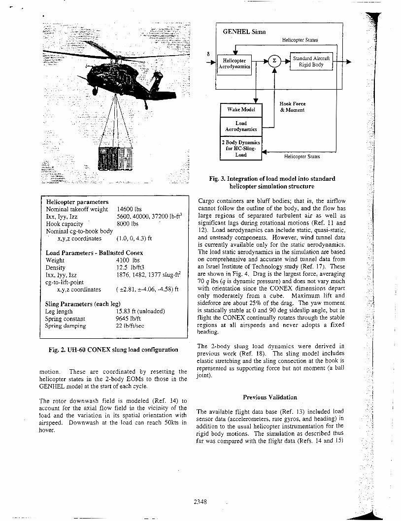
The simulation model was previously implemented at NASA Ames Research Center (Refs. 14 and 15), and is comprised of the GENHEL helicopter simulation (Ref. 16), the load aerodynamic model, and the slung load equations of motion. The structure of the simulation is outlined in Fig. 3. The original GENHEL sirnulation consists of the helicopter aerodynamics and the aircraft rigid body dynamics. The slung load aerodynamics, and Z-body equations of motion are appended to this as shown. There are two copies of the helicopter rigid body dynamics; one set in the GENHEL model and a second set in the 2-body equations of

2347

... . __ . ...... . . . . . -~ .. .-. .... . . . . . . . . . . . Standard Aircraft

Rigid Body Helicopter

Aerodynamics

t

. .... . . . ...... ~ - - .' ... . . :, -

......... ........ ~ . . . . .

-b

Helicopter parameters Nominal takeoff weizht 14600 lbs Ixx, Iyy, Izz 5600,40000,37200 lb-ft' Hook capacity 8000 lbs Nominal cg-to-hook body

x,y,z coordinates (1 .O, 0,4.3) ft

v Wake Model

Load

Load Parameters - Ballasted Conex Weight 4100 lbs Density 12.5 lb/ft3 Ixx, Iyy, Izz cg-to-lift-point

1876, 1482, 1377 slug-ft2

( 52.81, 5-4.06, -4.58) ft x.y,z coordinates

Hook Force & Moment

Sling Parameters (each leg) Leg length 15.83 ft (unloaded) Spring constant 9645 lb/ft Spring damping 22 lblftlsec

Aerodynamics

Fig. 2. UH-60 CONEX slung load configuration

-

motion. These are coordinated by resetting the helicopter states in the 2-body EOMs to those in the GENHEL model at the start of each cycle.

2 Body Dynamics for HC-Sling-

Load

The rotor downwash field is modeled (Ref. 14) to account for the axial flow field in the vicinity of the load and the variation in its spatial orientation with airspeed. Downwash at the load can reach 50kts in hover.

I Helicopter States

GENHEL Sinin i Helicopter States

c--------------.l I

Fig. 3. Integration of load model into standard helicopter simulation structure

Cargo containers are bluff bodies; that is, the airflow cannot follow the outline of the body, and the flow has large regions of separated turbulent air as well as significant lags during rotational motions (Ref. 11 and 12). Load aerodynamics can include static, quasi-static, and unsteady components. However, wind tunnel data is currently available only for the static aerodynamics. The load static aerodynamics in the simulation are based on comprehensive and accurate wind tunnel data from an Israel Institute of Technology study (Ref. 17). These are shown in Fig. 4. Drag is the largest force, averaging 70 q Ibs ( q is dynamic pressure) and does not vary much with orientation since the CONEX dimensions depart only moderately from a cube. Maximum lift and sideforce are about 25% of the drag. The yaw moment is statically stable at 0 and 90 deg sideslip angle, but in flight the CONEX continually rotates through the stable regions at all airspeeds and never adopts a fixed heading.

The 2-body slung load dynamics were derived in previous work (Ref. 18). The sling model includes elastic stretching and the sling connection at the hook is represented as supporting force but not moment (a ball joint).

Previous Validation

The available flight data base (Ref. 13) included load sensor data (accelerometers, rate gyros, and heading) in addition to the usual helicopter instrumentation for the rigid body motions. The simulation as described thus far was compared with the flight data (Refs. 14 and 15)

2348

1001 I

N

Y L

CY ij

a = -90,-80....,90 0

a = -90,-80,...,90 -30

Sideslip deg 30

20 Lift

Roll Moment p.) c Y 20

Yaw Moment Corrections

2349

One way to capture the observed yaw motions in the sirnulation i s to add empirical terms to the load and hook yaw moments to represent the effects just described, and then to tune the constants of the empirical terms to flight data. These terms were developed first as a 1-DOF model of the yaw motions:

r I , = YMsraric + AYM (1)

The lateral DOF was neglected because the yaw motions seen in flight for the CONEX were independent of the pendulum motions at the test airspeeds. The postulated yaw moment correction terms are:

where:

and where q is dynamic pressure, Vu is airspeed in kts, and r is yaw rate. YMslaric is the static aerodynamic yaw moment from Fig. 4. This varies with angle of attack and sideslip, a /3. Realistic values of a p were generated in the I-DOF simulation from trigonometric identities as a function of the nominal load trail angle and the load heading.

The sling windup resistance torque function, f ( A y ) , was measured in the laboratory. The CONEX and sling were suspended from overhead rails. The sling apex clevis was held fixed in place and a motor mounted underneath to turn the container. Measurements were recorded of the turn angle, torque, and sling geometry. The data for torque versus number of turns (Fig. 5) has a peak during the first turn as the clevis rotates to a stop against the hook and the sling leg windup begins, and subsequently the torque increases monotonically over the range of the test. Significant hysteresis is evident. These data were simulated as the average of the two curves at each rotation (dashed line in Fig. 5) , but this led to divergent windup in the simulation. Consequently, a damping term was added to obtain stable windup. This damping approximates the effect of hysteresis, since the resistance torque during windup is higher than the average curve at each rotation angle (hence less peak windup), and.restoring torque during the unwind is lower than the average curve (hence less peak yaw rate).

The vortex shedding term, YM,,,, is represented as a moment that switches sign with yaw rate. It increases

0 2 4 6 8 10 12 turns

Fig. 5. Lab measurement of sling windup

with dynamic pressure, acts in the same direction as the yaw rate (Le., is a propelling moment) and is continually active. This simple model has only one parameter whose value was obtained by tuning the model to the no-swivel flight data given the hook resistance function, RAW). An alternate 2-DOF empirical model of vortex shedding which captures the momentary nature of vortex shedding and includes lateral motions was proposed in (Ref. 8) for the MILVAN.

Swivel friction was difficult to measure in the laboratory, so the value of K, was estimated by tuning the model to the flight steady state yaw rates, given the vortex shedding parameter, K,,,, obtained from the no- swivel tuning.

The swirl correction, YM,,,,,, is a constant which fades out with airspeed near hover. The minus sign reflects the counter clockwise rotation of the wake. The value of AYM,,v,,l was obtained by tuning the model to the hover steady state yaw rate for the swiveled sling. given the swivel friction, K,.

The tuning resulted in values for the constants

Kdyn = 0.3 ft3

K,' = 3.0 f t - lbs -sec

K , = 1.2 ft - Ibs - sec

AYMs,v,rl = 1.0 ft - Ibs

(4)

These values reflect very small correction moments and indicate a strong effect on steady state yaw motions from small moments. The swiveled sling parameters were determined indirectly from the yaw resistance function for the unswiveled sling, and may contain errors. Nevertheless, steady state yaw rate for the

i

1 I

I I

I

I

I -

swiveled sling depends on a ratio of parameters and can be matched provided the ratio Is correctly obtained, as is shown next.

The 1-DOF equation for the swivel case is approximately a linear first order differential equation for which an approximate solution can be given. In hover the static and dynamic yaw moments are zero. In forward flight the dynamic term is a constant in steady state, and the static term was found to average to zero each rotation so that its influence on steady state could be neglected. This yields:

rss = fwd flight K d y 4

K r

(5)

Thus, steady state yaw rate depends only on the ratio of tuning constants while the transient response time constant depends on the magnitude of the swivel friction and is 1100 secs for the present parameter values. Suitable transient response flight data were not available to confirm the swivel friction estimate.

A comparison of yaw rate for the corrected simulation model and flight is shown in Fig. 6. The yaw rates plotted are steady state with a swivel, and the amplitude in the case of no swivel. Yaw rate magnitudes are significantly higher with the swivel. The available flight data have a large gap in airspeed between hover and 40 kts, so that the fitting function in the interior of this range has reduced confidence. Nevertheless, the tuned model reproduces the available flight steady state data reasonably well.

I

i

3 -80 - E E -100- %

-1401 -'zo\

-160 ' 0 10 20 30 40 50 60 70

true airspeed kts

Fig. 6. Simulation-flight comparison of steady state yaw rate

The yaw moment corrections were implemented in the GENHEL - slung load simuiation. Steady state results agreed closely with the 1-DOF results at all airspeeds, indicating that the 1-DOF model is a good approximation of load yaw in the 12-DOF 2-body simulation with the CONEX load. A comparison of yaw time histories with flight data for both the swiveled and unswiveled sling is shown in Fig. 7. The comparison shows good agreement in gross behavior, although there is some mismatch in windup amplitude for the unswiveled case. Some mismatch of the small scale variations (associated with rotations of the load through the static aerodynamics functions in Fig. 4 is visible for the swiveled sling: the frequency of these variations is matched, and differences in amplitude are likely due to unmodeled aerodynamic lags.

time - secs

Fig. 7. Load yaw rate - GenHeYflight comparison

Stabilizer Model

A vertical fin stabilizer and its geometry are shown in Fig. 8. The fin can be passive, adding static stability, or active with a control surface using yaw rate feedback to increase yaw damping. For this study, the control surface was taken at 25% of the chord with a 20 deg deflection limit. The simulation model included both horizontal and vertical fins for generality, but only results for the vertical fin are presented here.

The stabilizer aerodynamic model is taken from a study of flat plate aerodynamics in (Ref. 19) and is defined at all orientation angles. Flow direction relative to the fin is divided into distinct regions according to angle of attack as shown in Fig. 9 The pre-stall region ( a < as,) is characterized by circulation flow and thin airfoil theory where drag is due to skin friction and the center of pressure (c.P.) is at 25% chord. In the crossflow region (a > an). the fin is approximately broadside to

235 1

Fig. 8. Load fin stabilizer

--

a - aS2 transition as,* cross

- as1

pre-stall

\\sition

I

Nominal values: X, =8 f t Z v = 6 f t

b = 5 n c = 3 n

NACA 0015 airfoil .02

CD, .8 CLYD' 5.73 per radian

coo

as 1 20°

as2 4 5 O

Active stabilizer:

CLrD) 1.43 per radian KA .3 sec

Fig. 9. Stabilizer flow regions and parameters

the wind with separated flow and vortex effects, the principal force is pressure drag, and the c.p. is at 50% chord. In the transition region (as, < 01 < as2), forces and c.p. location are varied linearly. The aerodynamics above a = 90 deg is a mirror image of that below 90 deg. A typical airfoil, NACA 0015, was used and parameter values for its aerodynamic model are included in Fig. 9. Additional details of the stabilizer aerodynamic model can be found in (Refs. 19 and 20).

Moments about the CONEX center due to the fin are shown in Fig. 10. These are given as components in the CONEX body axes. They are computed for the example 15 ft?. fin dimensions and location of Fig. 8 and reflect principally the fin drag and lift forces acting at moment arms X , , 2,. Roll moment is about 75% of yaw moment. Pitching moment is small, under 10% of the peak yaw moment. Yaw moment due to the fin is globally statically stable only around p = 0. The CONEX static yaw moment is included in the figure for comparison; it is locally statically stable at p = 0, 90, 1SO deg and has peak moments only about 50% of the

J

i U r . I -50 5l -

-1 00

100

-' 50 Q 0

-50

100

Fig. 10. CONEX moments due to vertical fin stabilizer

2352

yaw moments and impose static stability at p = 0. Since both moments scale with dynamic pressure, then the same ratio of fin and CONEX static yaw moments will occur at all airspeeds.

(a) load yaw rate, swiveled sling peak fin yaw moment. Thus. for the example fin area and location, the fin can dominate the CONEX static loo

J

The present work models the fin aerodynamics as that of a thin wing in the freestream. While box-shaped loads have substantial wakes with low velocity turbulent air extending behind the entire rear surface of the container, the fin in this study is located above the container and its wake.

Results

In the absence of a fin, the simulation indicates instability above 80 kts for the 4000 Ib CONEX. This is seen as large pitch or roll oscillations approaching 90 deg. The actual mode of instability of the CONEX is not yet documented from wind tunnel studies or field data.

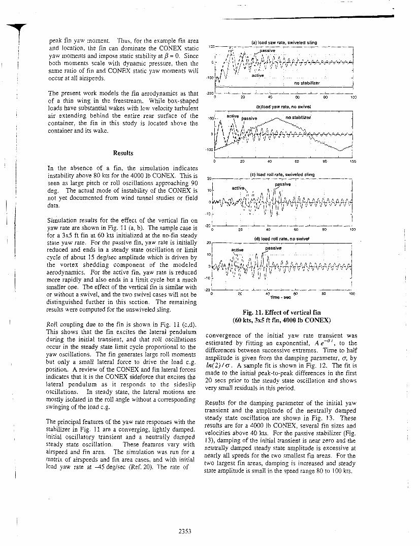
Simulation results for the effect of the vertical fin on yaw rate are shown in Fig. 11 (a, b). The sample case is for a 3x5 ft fin at 60 kts initialized at the no-fin steady state yaw rate. For the passive fin, yaw rate is initially reduced and ends in a steady state oscillation or limit cycle of about 15 degkec amplitude which is driven by the vortex shedding component of the modeled aerodynamics. For the active fin. yaw rate is reduced more rapidly and also ends in a limit cycle but a much smaller one. The effect of the vertical fin is similar with or without a swivel, and the two swivel cases will not be distinguished further in this section. The remaining results were computed for the unswiveled sling.

Roll coupling due to the fin is shown in Fig. I1 (c,d). This shows that the fin excites the lateral pendulum during the initial transient, and that roll oscillations occur in the steady state limit cycle proportional to the yaw oscillations. The fin generates large roll moments but only a small lateral force to drive the load c.g. position. A review of the CONEX and fin lateral forces indicates that it is the CONEX sideforce that excites the lateral pendulum as it responds to the sideslip oscillations. In steady state, the lateral motions are mostly isolated in the roll angle without a corresponding swinging of the load c.g.

The principal features of the yaw rate responses with the stabilizer in Fig. 11 are a converging, lightly damped, initial oscillatory transient and a neutrally damped steady state oscillation. These features vary with airspeed and fin area. The simulation was run for a matrix of airspeeds and fin area cases. and with initial load yaw rate at 4 5 deghec (Ref. 20). The rate of

!

no stabilizer I

-I I

.zoo ' I ,

60 80 100 20 40

(b)load yaw rate, no swivel

I 0 60 80 100 20 40

(C) load roll rate, swiveled sling 20,

I

0 ' d I -20

40 60 80 100 20

I I

0 60 80 100 20 40 -20

time - sec

Fig. 11. Effect of vertical fin (60 kts, 3x5 ft fin, 4000 Ib CONEX)

convergence of the initial yaw rate transient was estimated by fitting an exponential, A e-uf, to the differences between successive extremes. Time to half amplitude is given from the damping parameter, 0, by Zn(2)/0. A sample fit is shown in Fig. 12. The fit is made to the initial peak-to-peak differences in the first 20 secs prior to the steady state oscillation and shows very small residuals in this period.

Results for the damping parameter of the initial yaw transient and the amplitude of the neutrally damped steady state oscillation are shown in Fig. 13. These results are for a 4000 Ib CONEX, several fin sizes and velocities above 40 kts. For the passive stabilizer (Fig. 13), damping of the initial transient is near zero and the neutrally damped steady state amplitude is excessive at nearly all speeds for the two smallest fin areas. For the two largest fin areas, damping is increased and steady xate amplitude is small in the speed range 80 to 100 kts.

2353

I 0 10 20 30 40 50 60 70

time - sec

Fig. 12. Exponential envelope of initial settling transient (90 kts, 3x5 ft passive stabilizer)

(a) passive stabilizer

o i i u 40 60 80 100 120

u g 80 . 0) 60

- 31 40

; 20 P

40 60 80 100 120

airspeed - kts

(b) active stabilizer

40 60 BO 100 120

40

20

0 40 60 80 100 120

airspeed - Ms

Fig. 13. Damping and steady state results vs airspeed

Above 100 kts, steady state amplitude increases and effectiveness is lost at 120 kts in that the neutrally damped steady state oscillation dominates the motion. At low speed, effectiveness is also reduced as seen in a reduction of damping as airspeed decreases, and increased steady state amplitude. Performance for the two largest fins is nearly identical, so the 3x5 ft fin is the smallest passive stabilizer size tested with adequate performance.

The active stabilizer (Fig. 13) shows similar damping trends; that is, damping increases with airspeed above 60 kts until effectiveness is lost at 120 kts. Damping is double that of the passive stabilizer. Steady state amplitude increases above 100 kts, becoming excessive

0 ) ' I

40 60 EO 100 120

(b) steady alate yaw rate amplitude. deq'sec 50 ,

40 60 80 100 120

airspeed - kts

Fig, 14. Comparison of active and passive 3x5 ft stabilizers

at 120 kts as for the passive stabilizer. Steady state amplitude also increases at some low airspeeds. Again, the two largest fin areas have about the same performance at all airspeeds and better darnping than the two smallest fin areas at all airspeeds. These results indicate that stabilization can be achieved out to 110 kts and that a suitable fin size is 15 ft2 for the test load weight. Fig. 14 compares the passive and active 3x5 ft stabilizer. The benefit of the active stabilizer is significantly better damping at all airspeeds and lower steady state amplitude below 80 kts. However, it requires the addition of sensor, power source, and actuators to the fin design.

Factors limiting forward speed

The potential operational envelope of the stabilized load is limited by a variety of factors, which include the hook force limit, the maximum continuous power limit, control saturation, attitude limits, and structural limits.

The load has a significant effect on helicopter trim requirements, principally on trim power, collective, and pitch angle. Data are shown in Fig. 15 at high forward speeds for no load and various load weights. These data reflect the UH-60 aircraft with nominal parameter values (Fig. 2) and the CONEX load at 2000 ft altitude, standard atmosphere. Significant increases in power required are due to load drag (D*V/550). Since load drag is independent of load weight, increases in power requirements are similar at all load weights. Maximum continuous power (loo%, 2828 HP) is reached between 110 and 120 kts. Pitch attitude decreases due to the load (inversely with load weight), while collective setting increases with load weight, and these effects increase with airspeed. The pitch and collective trends reflect

2354

T I

J

i

i 1 f I

I

I

1

j

0 ' J 100 120 60 80

'5 10

100 120 60 80

lo- 8K = WL

100 120

True airspeed - kts

Fig. 15. Effect of load on helicopter trim

L

SHP limit

I

I

I I

I

I I I

1 I I

operational I

I 6000; limit (no fin) I

P 0

I empty CONEX Weight I the rotor thrust vector variations in inertial direction and magnitude required to balance the weight and drag forces of the helicopter and load. Pitch attitude limits for the helicopter (+/-30deg) are not encountered in this speed range, but collective will reach its 10-in limit between 120 and 130 kts for the load weights shown.

Some load weight-airspeed limits are collected in Fig. 16. The hook is certified to carry 8000 Ibs out to

True airspeed - Ms

Fig. 17. Load trail angle contours at high forward speeds

140 kts. This includes a margin to accommodate hook force increases above the load weight due to load drag and maneuvering acceleration. As noted above, maximum continuous power is reached between 110 and 120 kts and the collective is saturated at slightly higher airspeeds. A review of the relevant structural limits was omitted from this survey for lack of time. The operational speed limit for the CONEX, 60kts, is noted in the figure, and, in principal, stabilization can potentially extend the speed range to the power limit at about 115 kts.

Load drag causes the load to trail rearward in steady forward flight, increasing with airspeed. While there is no hard limit on trail angle, larger trail angles are a concern since they bring the load closer to the aircraft. The region above 60 kts is mapped for trail angle from the vertical (8, = tan-'(D/ W L ) ) in Fig. 17. At a given airspeed, lower container weights imply larger trail angles. For the CONEX, drag is unaffected by fin stabilization to a desired orientation since the CONEX is nearly cubic and drag varies only a little with orientation. This would not be the case for elongated containers, such as the MILVAN, where there is a potential 50% drag reduction by stabilizing at the minimum drag orientation. These contours indicate that large trail angles will occur at the lowest weights in extending the speed envelope past 100 kts. However, the angle relative to the helicopter vertical is somewhat less than the trail angle owing to the forward pitch of the helicopter (Fig. 15).

2355

1 3 . . Discussion References

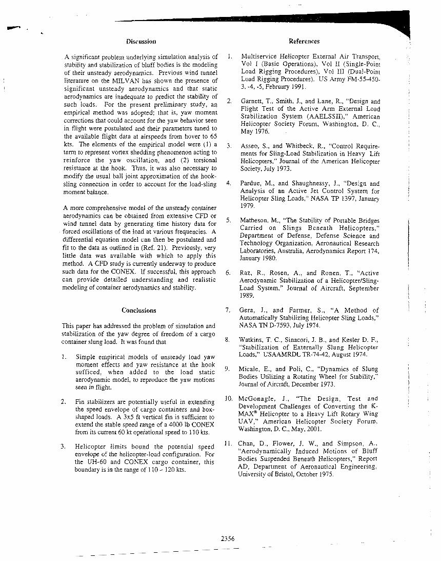
A significant problem underlying simulation analysis of stability and stabilization of bluff bodies is the modeling of their unsteady aerodynamics. Previous wind tunnel literature on the MILVAN has shown the presence of significant unsteady aerodynamics and that static aerodynamics are inadequate to predict the stability of such loads. For the present preliminary study, an empirical method was adopted; that is, yaw moment corrections that could account for the yaw behavior seen in flight were postulated and their parameters tuned to the available flight data at airspeeds from hover to 65 kts. The elements of the empirical model were (1) a term to represent vortex shedding phenomenon acting to reinforce the yaw oscillation, and (2) torsional resistance at the hook. Thus, it was also necessary to modify the usual ball joint approximation of the hook- sling connection in order to account for the load-sling moment balance.

A more comprehensive model of the unsteady container aerodynamics can be obtained from extensive CFD or wind tunnel data by generating time history data for forced oscillations of the load at various frequencies. A differential equation model can then be postulated and fit to the data as outlined in (Ref. 21). Previously, very little data was available with which to apply this method. A CFD study is currently underway to produce such data for the CONEX. If successful, this approach can provide detailed understanding and realistic modeling of container aerodynamics and stability.

Conclusions

This paper has addressed the problem of simulation and stabilization of the yaw degree of freedom of a cargo container slung load. It was found that

1. Simple empirical models of unsteady load yaw moment effects and yaw resistance at the hook sufficed, when added to the load static aerodynamic model, to reproduce the yaw motions seen in flight.

Fin stabilizers are potentially useful in extending the speed envelope of cargo containers and box- shaped loads. A 3x5 ft vertical fin is sufficient to extend the stable speed range of a 4000 lb CONEX from its current 60 kt opeiational speed to 110 kts.

2 .

3. Helicopter limits bound the potential speed envelope of the helicopter-load configuration. For the UH-60 and CONEX cargo container, this boundary is in the range of 110 - 120 kts.

1.

2.

3.

4.

5 .

6.

7.

8.

9.

10.

11.

Multiservice Helicopter External Air Transport, Vol I (Basic Operations), Vol I1 (Single-Point Load Rigging Procedures), Vol I11 (Dual-Point Load Rigging Procedures). US Army FM-55-450- 3. -4, -5 , February 1991.

Garnett, T., Smith, J., and Lane, R., “Design and Flight Test of the Active Arm External Load Stabilization System (AAELSSII),” American Helicopter Society Forum, Washington, D. C., May 1976.

Asseo, S., and Whitbeck, R., “Control Require- ments for Sling-Load Stabilization in Heavy Lift Helicopters,” Journal of the American Helicopter Society, July 1973.

Pardue, M., and Shaughnessy, J., “Design and Analysis of an Active Jet Control System for Helicopter Sling Loads,” NASA Tp 1397, January 1979.

Matheson, M., “The Stability of Portable Bridges Carried on Slings Beneath Helicopters.” Department of Defense, Defense Science and Technology Organization, Aeronautical Research Laboratories, Australia, Aerodynamics Report 174, January 1980.

Raz, R., Rosen, A., and Ronen, T., “Active Aerodynamic Stabilization of a Helicopter/Sling- Load System,” Journal of Aircraft, September 1989.

Gera, J., and Farmer, S., “A Method of Automatically Stabilizing Helicopter Sling Loads,”

Watkins, T. C., Sinacori, J. B., and Kesler D. F., “Stabilization of Externally Slung Helicopter Loads,” USAAMRDL TR-74-42, August 1974.

Micale, E., and Poli, C., “Dynamics of Slung Bodies Utilizing a Rotating Wheel for Stability,” Journal of Aircraft, December 1973.

NASA TN D-7593, July 1974.

McGonagle, J., “The Design, Test and Development Challenges of Converting the K- MAX@ Helicopter to a Heavy Lift Rotary Wing UAV,“ American Helicopter Society Forum, Washington, D. C., May, 2001.

Chan, D., Flower, J. W., and Simpson, A., “Aerodynamically Induced Motions of Bluff Bodies Suspended Beneath Helicopters,” Report AD, Department of Aeronautical Engineering, University of Bristol, October 1975.

I : I :

‘ I

12. Simpson, A., and Flower, 1. W., “Unsteady Aerodynamics of Oscillating Containers and Application to the Problem of Dynamic Stability of Helicopter Underslung Loads,“ AGARD CP-235, May 1978.

13. Cicolani, L., McCoy, A., Sahai, R., Tyson. P., Tischler, M., Rosen, A., and Tucker G., “Flight Test Identification and Simulation of a UH-60A Helicopter and Slung Load.,” NASA TM-2001- 209619, January 2001; also Journal of the American Helicopter Society, April 2001.

14. Tyson, P., Cicolani, L., Tischler, M., Rosen, A., Levine, D.. and Dearing, M., “Simulation Prediction and Flight Validation of UH-60A Black Hawk Slung Load Characteristics,” American Helicopter Society Forum, Montreal. May 1999.

15. Tyson, P., “Simulation Validation and Flight Prediction o f UH-60A Black Hawk Helicopter/Slung Load Characteristics,” MS Thesis, US Naval Postgraduate School, Department of Aeronautics and Astronautics, Monterey, CA, March 1999.

16. Howlett, J., “UH-60A Black Hawk Engineering Simulation Program,” NASA CR 166309, December 1981.

i7

18.

19.

20.

21.

Rosen, A.. Cecutta. S.. Yaffe, R., “Wind Tunnel Tests of Cube and CONEX models,” Technion Institute of Technology, Department of Aerospace Engineering. TAE844, November 1999.

Cicolani, L.. Kanning, G., “Equations of Motion of Slung Load Systems, Including Multilift Systems,” NASA TP 3280, November 1992.

Tischler, M., Ringland, R., Jex, H., Emmen, R., and Ashkenas, I., “Flight Dynamics Analysis and Simulation of Heavy Lift Airships,” NASA CR 166471, December 1982.

Ehlers, G., “Hi-fidelity Simulation and Prediction of Helicopter Single Point External Load Stabilization,” MS Thesis, US Naval Postgraduate School, Department of Aeronautics and Astronautics, Monterey, CA. September 2001.

Ronen, T., Bryson, A., and Hindson, W., “Dynamics of a Helicopter with a Sling Load,” AIAA Atmospheric Flight Mechanics Conference, August 1986.

2357