Modeling and Forecasting the Impact of Major Technological ... · Modeling and Forecasting the...

Modeling and Forecasting the Impact of Major Technological

and Infrastructural Changes on Travel Demand

By

Feras El Zarwi

A dissertation submitted in partial satisfaction of the

requirements for the degree of

Doctor of Philosophy

in

Engineering – Civil and Environmental Engineering

in the

Graduate Division

of the

University of California, Berkeley

Committee in charge:

Professor Joan Walker, Chair

Professor Mark Hansen

Professor Paul Waddell

Professor Maximilian Auffhammer

Spring 2017

http://www.auffhammer.com/

1

Abstract

Modeling and Forecasting the Impact of Major Technological

and Infrastructural Changes on Travel Demand

By

Feras El Zarwi

Doctor of Philosophy in Engineering – Civil and Environmental Engineering

University of California, Berkeley

Professor Joan Walker, Chair

The transportation system is undergoing major technological and infrastructural changes, such as

the introduction of autonomous vehicles, high speed rail, carsharing, ridesharing, flying cars,

drones, and other app-driven on-demand services. While the changes are imminent, the impact on

travel behavior is uncertain, as is the role of policy in shaping the future. Literature shows that

even under the most optimistic scenarios, society’s environmental goals cannot be met by

technology, operations, and energy system improvements only – behavior change is needed.

Behavior change does not occur instantaneously, but is rather a gradual process that requires years

and even generations to yield the desired outcomes. That is why we need to nudge and guide trends

of travel behavior over time in this era of transformative mobility. We should focus on influencing

long-range trends of travel behavior to be more sustainable and multimodal via effective policies

and investment strategies. Hence, there is a need for developing policy analysis tools that focus on

modeling the evolution of trends of travel behavior in response to upcoming transportation services

and technologies. Over time, travel choices, attitudes, and social norms will result in changes in

lifestyles and travel behavior. That is why understanding dynamic changes of lifestyles and

behavior in this era of transformative mobility is central to modeling and influencing trends of

travel behavior. Modeling behavioral dynamics and trends is key to assessing how policies and

investment strategies can transform cities to provide a higher level of connectivity, attain

significant reductions in congestion levels, encourage multimodality, improve economic and

environmental health, and ensure equity.

This dissertation focuses on addressing limitations of activity-based travel demand models in

capturing and predicting trends of travel behavior. Activity-based travel demand models are the

commonly-used approach by metropolitan planning agencies to predict 20-30 year forecasts.

These include traffic volumes, transit ridership, biking and walking market shares that are the

2

result of large scale transportation investments and policy decisions. Currently, travel demand

models are not equipped with a framework that predicts long-range trends in travel behavior for

two main reasons. First, they do not entail a mechanism that projects membership and market share

of new modes of transport into the future (Uber, autonomous vehicles, carsharing services, etc).

Second, they lack a dynamic framework that could enable them to model and forecast changes in

lifestyles and transport modality styles. Modeling the evolution and dynamic changes of behavior,

modality styles and lifestyles in response to infrastructural and technological investments is key to

understanding and predicting trends of travel behavior, car ownership levels, vehicle miles traveled

(VMT), and travel mode choice. Hence, we need to integrate a methodological framework into

current travel demand models to better understand and predict the impact of upcoming

transportation services and technologies, which will be prevalent in 20-30 years.

The objectives of this dissertation are to model the dynamics of lifestyles and travel behavior

through:

Developing a disaggregate, dynamic discrete choice framework that models and predicts long-

range trends of travel behavior, and accounts for upcoming technological and infrastructural

changes.

Testing the proposed framework to assess its methodological flexibility and robustness.

Empirically highlighting the value of the framework to transportation policy and practice.

The proposed disaggregate, dynamic discrete choice framework in this dissertation addresses two

key limitations of existing travel demand models, and in particular: (1) dynamic, disaggregate

models of technology and service adoption, and (2) models that capture how lifestyles, preferences

and transport modality styles evolve dynamically over time. This dissertation brings together

theories and techniques from econometrics (discrete choice analysis), machine learning (hidden

Markov models), statistical learning (Expectation Maximization algorithm), and the technology

diffusion literature (adoption styles). Throughout this dissertation we develop, estimate, apply and

test the building blocks of the proposed disaggregate, dynamic discrete choice framework. The

two key developed components of the framework are defined below.

First, a discrete choice framework for modeling and forecasting the adoption and diffusion of new

transportation services. A disaggregate technology adoption model was developed since models

of this type can: (1) be integrated with current activity-based travel demand models; and (2)

account for the spatial/network effect of the new technology to understand and quantify how the

size of the network, governed by the new technology, influences the adoption behavior. We build

on the formulation of discrete mixture models and specifically dynamic latent class choice models,

which were integrated with a network effect model. We employed a confirmatory approach to

estimate our latent class choice model based on findings from the technology diffusion literature

that focus on defining distinct types of adopters such as innovator/early adopters and imitators.

Latent class choice models allow for heterogeneity in the utility of adoption for the various market

segments i.e. innovators/early adopters, imitators and non-adopters. We make use of revealed

preference (RP) time series data from a one-way carsharing system in a major city in the United

States to estimate model parameters. The data entails a complete set of member enrollment for the

carsharing service for a time period of 2.5 years after being launched. Consistent with the

technology diffusion literature, our model identifies three latent classes whose utility of adoption

3

have a well-defined set of preferences that are statistically significant and behaviorally consistent.

The technology adoption model predicts the probability that a certain individual will adopt the

service at a certain time period, and is explained by social influences, network effect, socio-

demographics and level-of-service attributes. Finally, the model was calibrated and then used to

forecast adoption of the carsharing system for potential investment strategy scenarios. A couple of

takeaways from the adoption forecasts were: (1) highest expected increase in the monthly number

of adopters arises by establishing a relationship with a major technology firm and placing a new

station/pod for the carsharing system outside that technology firm; and (2) no significant difference

in the expected number of monthly adopters for the downtown region will exist between having a

station or on-street parking.

The second component in the proposed framework entails modeling and forecasting the evolution

of preferences, lifestyles and transport modality styles over time. Literature suggests that

preferences, as denoted by taste parameters and consideration sets in the context of utility-

maximizing behavior, may evolve over time in response to changes in demographic and situational

variables, psychological, sociological and biological constructs, and available alternatives and

their attributes. However, existing representations typically overlook the influence of past

experiences on present preferences. This study develops, applies and tests a hidden Markov model

with a discrete choice kernel to model and forecast the evolution of individual preferences and

behaviors over long-range forecasting horizons. The hidden states denote different preferences,

i.e. modes considered in the choice set and sensitivity to level-of-service attributes. The

evolutionary path of those hidden states (preference states) is hypothesized to be a first-order

Markov process such that an individual’s preferences during a particular time period are dependent

on their preferences during the previous time period. The framework is applied to study the

evolution of travel mode preferences, or modality styles, over time, in response to a major change

in the public transportation system. We use longitudinal travel diary from Santiago, Chile. The

dataset consists of four one-week pseudo travel diaries collected before and after the introduction

of Transantiago, which was a complete redesign of the public transportation system in the city.

Our model identifies four modality styles in the population, labeled as follows: drivers, bus users,

bus-metro users, and auto-metro users. The modality styles differ in terms of the travel modes that

they consider and their sensitivity to level-of-service attributes (travel time, travel cost, etc.). At

the population level, there are significant shifts in the distribution of individuals across modality

styles before and after the change in the system, but the distribution is relatively stable in the

periods after the change. In general, the proportion of drivers, auto-metro users, and bus-metro

users has increased, and the proportion of bus users has decreased. At the individual level, habit

formation is found to impact transition probabilities across all modality styles; individuals are more

likely to stay in the same modality style over successive time periods than transition to a different

modality style. Finally, a comparison between the proposed dynamic framework and comparable

static frameworks reveals differences in aggregate forecasts for different policy scenarios,

demonstrating the value of the proposed framework for both individual and population-level policy

analysis.

The aforementioned methodological frameworks comprise complex model formulation. This

however comes at a cost in terms of prolonged computation and estimation times. Due to the non-

convex nature of the objective function, direct maximization of the likelihood could become

4

difficult and highly unstable. An alternative approach would be to use the Expectation

Maximization (EM) algorithm instead of traditional gradient descent algorithms. This particular

statistical learning technique is more stable, and requires fewer iterations to converge by taking

advantage of the conditional independence structure of the model framework. This dissertation

will provide rigorous derivation, formulation and application of the EM algorithm for mixture

models and hidden Markov models with logit kernels, which constitute the building blocks of the

generalized dynamic framework. Using such a statistical learning technique, i.e. the EM algorithm,

model estimation time will be reduced from the order of many hours to minutes.

The line of work initiated throughout this dissertation is critical in this era of transformative

mobility in terms of developing a generalized model that accounts for adoption styles and dynamic

modality styles. The proposed dynamic, disaggregate discrete choice framework models the

evolution of travel and activity behavior over time in addition to the adoption and diffusion of new

transportation services. The proposed framework can be integrated with current travel demand

models through the construct of adoption styles and modality styles, which shall provide a deeper

understanding of behavioral dynamics and trends of travel behavior in an attempt to better inform

long-range policy making. This dissertation provides the building blocks to advance the field of

travel demand modeling in order to guide transformative mobility into the envisioned sharing

economy future.

i

Table of Contents

List of Figures ............................................................................................................................... iii

List of Tables ................................................................................................................................ iv

Acknowledgements ....................................................................................................................... v

Chapter 1 Introduction................................................................................................................. 1

1.1 Motivation ............................................................................................................................. 1

1.2 Activity-based Travel Demand Models ................................................................................ 2

1.3 Discrete Choice Analysis and Random Utility Models ........................................................ 5

1.4 Behavioral Theory and Discrete Choice Analysis ................................................................ 7

1.5 Limitations of Activity-based Travel Demand Models in Capturing Trends of Travel

Behavior ...................................................................................................................................... 8

1.6 Objectives ............................................................................................................................ 10

1.7 Methodological Framework ................................................................................................ 10

1.8 General Overview of Model Framework in This Dissertation ............................................ 12

1.9 Dissertation Outline............................................................................................................. 14

1.10 Contributions ..................................................................................................................... 15

Chapter 2 A Discrete Choice Framework for Modeling and Forecasting the Adoption and

Diffusion of New Transportation Services ................................................................................ 17

2.1 Introduction ......................................................................................................................... 17

2.2 Literature Review ................................................................................................................ 19


2.4 Dataset ................................................................................................................................. 30

2.5 Estimation Results and Discussion ..................................................................................... 32

2.6 Policy Analysis .................................................................................................................... 37

2.7 Conclusion ........................................................................................................................... 45

Acknowledgements ................................................................................................................... 45

Chapter 3 Modeling and Forecasting the Evolution of Preferences over Time: A Hidden

Markov Model of Travel Behavior ............................................................................................ 46

3.1 Introduction ......................................................................................................................... 46

3.2 Motivation: Evolution of Individual Preferences over Time .............................................. 48

3.3 Methodological Basis: Dynamic Models for Discrete Choice Analysis ............................. 50


ii

3.4.1 Class-specific Mode Choice Model .............................................................................. 54

3.4.2 Initialization Model ...................................................................................................... 55

3.4.3 Transition Model .......................................................................................................... 56

3.4.4 Likelihood Function of the Full Model ........................................................................ 57

3.5 Initialization Problem in Dynamic Models ......................................................................... 58

3.6 Dataset ................................................................................................................................. 61

3.7 Estimation Results and Discussion ..................................................................................... 66

3.8 Policy Analysis .................................................................................................................... 72

3.9 Conclusion ........................................................................................................................... 75

Acknowledgements ................................................................................................................... 77

Chapter 4 Expectation Maximization Algorithm: Derivation and Formulation for Mixture

Models and Hidden Markov Models with Logit Kernels ........................................................ 78

4.1 Introduction ......................................................................................................................... 78

4.2 Mixture Models with Logit Kernels .................................................................................... 79

4.2.1 The EM Formulation .................................................................................................... 80

4.2.2 The E-step ..................................................................................................................... 81

4.2.3 The M-Step ................................................................................................................... 82

4.2.4 Gradient for Weighted Multinomial Logit Modal ........................................................ 82

4.3 Hidden Markov Models with Logit Kernels ....................................................................... 85

4.3.1 The EM Formulation .................................................................................................... 86

4.3.2 The E-step ..................................................................................................................... 87

4.3.3 The M-Step ................................................................................................................... 91

4.3.4 Gradient for Weighted Multinomial Logit Modal ........................................................ 92

4.4 Conclusion ........................................................................................................................... 93

Chapter 5 Conclusion ................................................................................................................. 94

5.1 Summary ............................................................................................................................. 94

5.2 Research Directions............................................................................................................. 98

5.3 Conclusion ......................................................................................................................... 100

Bibliography .............................................................................................................................. 102

iii

List of Figures Figure 1.1: Current and Upcoming Infrastructural and Technological Investments ..................... 2

Figure 1.2: SF-CHAMP Modeling Framework ............................................................................. 4

Figure 1.3: Standard Discrete Choice Framework......................................................................... 7

Figure 1.4: Decision Process (figure taken from McFadden, 1999) .............................................. 8

Figure 1.5: Proposed Disaggregate, Dynamic Discrete Choice Framework ............................... 11

Figure 2.1: Sales vs. Cumulative Sales over Time ...................................................................... 21

Figure 2.2: Latent Class Choice Model Framework .................................................................... 25

Figure 2.3: Generalized Technology Adoption Model ................................................................ 29

Figure 2.4: Cumulative Number of Adopters of Carsharing Service .......................................... 30

Figure 2.5: Growth in Number of Pods/Stations and On-Street Parking over Time ................... 31

Figure 2.6: Boxplots for Predicted Number of Adopters for Months 26-30 ............................... 37

Figure 2.7: Cumulative Adoptions for New Transportation Service ........................................... 38

Figure 2.8: Forecasted Adoption for New Transportation Service .............................................. 39

Figure 2.9: Boxplots for Predicted Cumulative Number of Adopters for Base Case Scenario ... 40

Figure 2.10: Boxplots for Predicted Cumulative Number of Adopters for Downtown On-Street

Parking Scenario ........................................................................................................................... 41

Figure 2.11: Boxplots for Predicted Cumulative Number of Adopters for Downtown Station

Scenario......................................................................................................................................... 42

Figure 2.12: Boxplots for Predicted Cumulative Number of Adopters for Major Technology

Firm ............................................................................................................................................... 43

Figure 2.13: Adopters vs. Cumulative Adopters over Time Using Bass Model ......................... 44

Figure 3.1: Hidden Markov Model Structure (figure adapted from Choudhury et al., 2010) ..... 52

Figure 3.2: Proposed Dynamic Discrete Choice Framework ...................................................... 53

Figure 3.3: Mode Shares across All Waves ................................................................................. 63

Figure 3.4: Shifts across Travel Modes between Subsequent Waves of the Panel ..................... 64

Figure 3.5: Estimated Share of Individuals in Each Modality Style across Waves ..................... 70

Figure 3.6: Estimated Average Transition Probabilities across Modality Styles over Time ....... 71

Figure 3.7: Share of Individuals in Each Modality Style for Policy Scenario 1, as Predicted by

the HMM, the LCCM Estimated Using Wave 1 Data, and the LCCM Estimated Using Wave 4

Data ............................................................................................................................................... 73

Figure 3.8: Mode Shares for Policy Scenario 1, as Predicted by the HMM, the LCCM Estimated

Using Wave 1 Data, and the LCCM Estimated Using Wave 4 Data ............................................ 73

Figure 3.9: Share of Individuals in Each Modality Style for Policy Scenario 2, as Predicted by

the HMM, the LCCM Estimated Using Wave 1 Data, and the LCCM Estimated Using Wave 4

Data ............................................................................................................................................... 74

Figure 3.10: Mode Shares for Policy Scenario 2, as Predicted by the HMM, the LCCM

Estimated Using Wave 1 Data, and the LCCM Estimated Using Wave 4 Data ........................... 74


Figure 4.2: Dynamic Discrete Choice Framework ...................................................................... 85

Figure 5.1: Proposed Disaggregate, Dynamic Discrete Choice Framework ............................... 95


Figure 5.3: Dynamic Discrete Choice Framework ...................................................................... 96

iv

List of Tables Table 2.1: Destination Choice Model .......................................................................................... 33

Table 2.2: Class Membership Model ........................................................................................... 34

Table 2.3: Class-specific Technology Adoption Model .............................................................. 35

Table 2.4: Measures of Model Fit ................................................................................................ 36

Table 3.1: Monte Carlo Simulation Results ................................................................................. 61

Table 3.2: Measures of Model Fit ................................................................................................ 66

Table 3.3: Class-specific Travel Mode Choice Model Results .................................................... 67

Table 3.4: Initialization Model Results ........................................................................................ 67

Table 3.5: Transition Model Results ............................................................................................ 68

v

Acknowledgements There are a lot of people that I would like to acknowledge in terms of their support and inspiration

prior to joining and throughout the PhD program at UC Berkeley.

My deepest gratitude goes to my favorite advisor, Professor Joan Walker. Thank you Joan for

sharing your knowledge, widening my horizon in the discrete choice modeling world, pushing me

further in research, and teaching me the importance of being extremely meticulous when it comes

to writing papers and giving talks. Thank you Joan for all the support and encouragement

throughout those three years of the PhD, and for your wonderful advice concerning tough career

choices.

I would also like to deeply thank Akshay Vij for the patience, support, and encouragement

throughout developing the algorithms I used in this dissertation and not to mention the great

feedback regarding the hidden Markov model research project. I would also like to thank the

members of my dissertation committee: Professor Mark Hansen, Professor Paul Waddell, and

Professor Maximilian Auffhammer for their great feedback and suggestions to further improve my

dissertation and its contributions.

Most importantly I am the most thankful to my amazing parents for their support, patience, and

love. To my amazing brothers and best friends Imad and Nader, I am very thankful for having you

in my life and for being great support pillars throughout this PhD process. To my wonderful

grandmother, I owe you so much for always pushing me to pursue my PhD and for being my

biggest fan. To my dad and for all the sacrifices he made in his life to provide us with a decent and

fruitful future, and to my mum for being a great confidant that supported all of my decisions. I

hope I have made you guys proud.

To my best friends and childhood friends back home: Ruba, Jad, Hrayer, Mira, Zeina, Marwan,

and Carol, thanks for always being there and for encouraging me to pursue my PhD. You guys are

a great support system and have had fruitful impacts on my personal and academic lives. To my

AUB colleagues: Samar, Imad, Lisa, Anthony and Luna, thanks for being encouraging and

supportive of my decision to pursue the PhD, and I will never forget the brain-washing sessions

that happened in Beirut prior to joining the PhD program. To the amazing people and great friends

I made during my time at Berkeley. Sreeta: thanks for being there during the ups and downs of the

PhD and I am definitely grateful for this friendship. Timothy: couldn’t be happier to be teaching

you Arabic slang and will never forget those crazy moments of stress and great memories

throughout the PhD. Naty (my Consuelo): second year of the PhD would have never been the same

without you. Thanks for the guidance, support and the great moments we shared. Elly, Marco,

Mostafa, Apoorva and Tala: was great getting to know you guys and definitely thankful for all the

good times we’ve had. Tania, Fadi, and Abdulrahman: thanks for the good memories and

encouragement throughout the PhD. I would also like to thank everyone in 116 Mclaughlin and

the new graduate students in the transportation program for the good conversations, memories, and

continuous interest in my work: Maddie, Teddy, Emin, Andrew, Sid, Yanqiao, Stephen, Mengqiao,

Hassan, Amine, Jessica and Catalina.

http://www.auffhammer.com/

1

Chapter 1

Introduction

1.1 Motivation The growth in population and urban development has impacted societies in one way or another

from air pollution to greenhouse gas emission, climate change and traffic congestion. This in turn

encouraged more investments in infrastructure and technological services to take place. Behavioral

change in terms of motivating people towards the use of more sustainable modes of transport is

necessary to achieve the required reductions in traffic congestion and efficient usage of the

available infrastructure. And as we know people are at the heart of most of the issues in

metropolitan studies, in which prime objectives are to better understand and improve the urban

environment. The behavioral and decision-making process that individuals and consumers

undergo can’t be overlooked when it comes to evaluating a set of investment strategies or policies

aimed at improving sustainable mobility and multimodality. Modeling this decision-making

process is key to (1) identifying the most effective policy or investment strategy catered towards

behavioral change, (2) predicting and forecasting the demand of policies and investment strategies

for a certain population in a more representative manner, and (3) specifying sources of

heterogeneity in tastes and preferences.

Major investments in technology and infrastructure are expected to occur over the next decades

such as the introduction of autonomous vehicles, connected vehicles, high speed rail, carsharing

and ridesharing. This shall induce potential paradigm shifts in the cost, speed, safety, convenience

and reliability of travel. Together, they are expected to influence both short-term travel and activity

decisions, such as where to go and what mode of travel to use, and more long-term travel and

activity decisions, such as where to live and how many cars to own. This transformative mobility

trend, whether in the form of sharing economy, connected vehicles, autonomous and app-driven

on-demand vehicles and services will impact travel and activity behavior through disrupting the

need to travel and the disutility of travel. While the changes are imminent, the impact on travel

behavior is uncertain as is the role that policy can play in shaping the outcome. We want the future

to consist of sustainable and efficient systems, which cannot be attained by technology, operations,

and energy system improvements only – behavior change is needed. Developing quantitative

behavioral analysis tools that focus on modeling and influencing trends of travel behavior to guide

transformative mobility and set it on the right track is a key ingredient. This is a critical component

in the design of smart cities that need to be shaped with the correct set of policies and regulations

to attain the desired goals and outcomes.

Moreover, the automobile has long been the preeminent mode of transportation, more so in the

United States (US) than anywhere else. However, the last decade has heralded a generational

change within much of the developed world in terms of attitudes towards the car. Between 2000

and 2010, in the US alone, car sales went down by 35.8 percent, per capita highway passenger

vehicle miles traveled (VMT) decreased by 6.7 percent, while the proportion of the driving age

population that is licensed to drive declined from 88.0 percent to 86.4 percent (Office of Highway

Policy Information). Researchers have referred to this process or phenomenon as “peak auto” with

2

the reversal in the car dependence being variously attributed to factors that include a stagnant

economy, an aging population, rising oil prices, a renewed interest in urbanism, growth in e-

commerce, the spread of online social network, and the smart phone revolution.

Figure 1.1: Current and Upcoming Infrastructural and Technological Investments

The impact of comparable changes in technology and infrastructure in the past has thus far been

examined retrospectively. A framework for predicting long-range trends in travel behavior, such

as the peak auto or the rise of carsharing and ridesharing, remains lacking. As a consequence,

transportation specialists, practitioners and policy-makers have been historically forced to be more

reactionary than visionary. That is why it is essential to develop quantitative methods for travel

demand analysis that can be used to understand and predict long-range trends in travel and activity

behavior in response to major infrastructural and technological changes affecting both the

transportation and land use system. Over time, travel choices, attitudes, and social norms will result

in changes in lifestyles and travel behavior. That is why understanding dynamic changes of

lifestyles and behavior in this era of transformative mobility is central to modeling and influencing

trends of travel behavior, and improving long-range forecasting accuracy.

1.2 Activity-based Travel Demand Models Activity-based travel demand models are the commonly-used approach by metropolitan planning

agencies to predict 20-30 year forecasts of traffic volumes, transit ridership, biking and walking

market shares brought about from large scale transportation investments and policy decisions.

These models try to assess the impacts of transportation investments, land use and socio-

demographic changes on travel behavior with the main objective of predicting future mode shares,

auto ownership levels, etc. These forecasts are critical in assessing the viability of any

infrastructure investment or policy (e.g., parking, HOV lanes, etc.) as they predict how decisions

now will play out in the future. Furthermore, results from these models will: (1) provide insight to

locations and corridors bound to suffer from congestion in future years, (2) identify impacts of a

3

certain infrastructure investment or policy in mitigating congestion along congested spines or

corridors, and (3) assess increase/reduction in greenhouse gas emissions (GHG). This dissertation

contributes to efforts that aim at addressing shortcomings of current activity-based travel demand

models in order to account for transformative technological and infrastructural changes.

This section provides a brief overview of the various components of activity-based travel demand

models. The strong relationship that exists between travel and activities comprises the basis for

these types of models (Bhat and Koppelman, 1999). Travel is assumed to be a derived demand

whereby people travel to participate in certain activities (shopping, work, recreational, etc.). The

figure below displays the modeling framework of the San Francisco Chained Activity Modeling

Process (SF-CHAMP). It is evident that several interdependent models make up the travel demand

modeling framework. Some of the key sub-models are described below:

a- Population Synthesizer

This component comprises microsimulation techniques as opposed to the traditional sample

enumeration methods. Microsimulation focuses on modeling the behavior of a sample of

individuals and households that are representative of the target population. A sample is created

that entails decision-makers and households with a set of socio-demographics and other

characteristics that match the designated population. The synthesized individuals are assigned

respectively to households, which have a defined list of characteristics (number of workers,

number of vehicles owned, etc.). Following that, households are mapped to various residential

locations that are in turn divided into travel analysis zones (TAZ).

b- Vehicle Availability Model

This component evaluates the auto ownership level for each of the households. The choice of

owning zero or multiple vehicles is modeled as a function of characteristics of the household.

c- Full-Day Tour Pattern Models

These types of models predict the tour patterns for each of the individuals in the population

synthesizer. Five types of tours are included in the SF-CHAMP framework:

i- Home-based work primary tours

ii- Home-based education primary tours

iii- Home-based other primary tours

iv- Home-based secondary tours

v- Work-based sub-tours

A home-based tour comprises the entire set of trips conducted by the time a decision-maker leaves

his/her house until he/she gets returns home. Primary versus secondary tours vary based on the trip

purpose. For example, education, work, shopping, personal business, social/recreation, and serve

passengers are considered as primary tours (Primerano, 2008). The remaining trip purposes are

considered as secondary.

4

Figure 1.2: SF-CHAMP Modeling Framework

5

d- Time of Day Models

This component models the start time, end time, and duration of all trips in a certain tour (Abou

Zeid et al., 2006). Models are estimated at two different levels. First level entails “modeling the

joint choice of arrival time at a primary destination of the tour and departure time from the primary

destination of the tour” while the second level comprises “modeling the arrival time at or departure

time from the intermediate stop and consequently its duration” (Abou Zeid et al., 2006).

e- Tour/Trip Mode Choice Models

This component models travel mode choice for various tours and trips. In other words,

probabilistic models are developed to predict the primary mode used for each of the available tours

in addition to each of the conducted trips. Choice set consideration for the trip mode choice consists

of available modes of transport.

The aforementioned models are typically specified as binary, multinomial or nested logit choice

models. Random utility models and in particular discrete choice analysis constitute the building

blocks of activity-based travel demand models.

1.3 Discrete Choice Analysis and Random Utility Models Discrete choice analysis (Ben-Akiva and Lernam, 1985) focuses on modeling a dependent variable

that takes on discrete values. Discrete choice modeling is widely used in the transportation industry

for travel demand modeling and forecasting. However, models of this kind are applicable to a wide

variety of businesses and public organizations, with the objective of better understanding and

predicting the demand and market shares for goods and services. These techniques are widely used

in market research and quantitative marketing. Of great interest is the identification of key

variables that shape the demand of a certain good/service, which include, but are not limited to,

characteristics of the decision-maker, attributes of the available alternatives, attitudes and

perceptions, as well as social influences.

Random utility models are based on the notion that decision-makers associate a “utility” with each

of the available alternatives in their consideration set. Utility is an abstract concept that tries to

quantify the level of attractiveness of a certain alternative (McFadden, 2001; Ben-Akiva and

Lerman, 1985). The decision-maker is postulated to choose the alternative that maximizes his/her

random utility. Other decision rules exist but utility maximization has been the decision rule of

choice for studies on individual and household travel and activity behavior. Note that utility is not

observed by the analyst, which is why it is treated as a random variable. Random utility is broken

down into an observable deterministic component and an unobservable component (adapted from

Walker, 2001):

𝑈𝑖𝑛 = 𝑉(𝑋𝑖𝑛; 𝛽) + 휀𝑖𝑛

where:

𝑈𝑖𝑛 denotes the random utility of an alternative i for individual n

V denotes the function that expresses the systematic/observable component of utility as a

function of explanatory variables

6

𝑋𝑖𝑛 denotes explanatory variables; attributes of alternative i and characteristics of individual n

𝛽 denotes the parameter vector to be estimated

휀𝑖𝑛 denotes the random/unobservable component of random utility

The most common class of discrete choice models is the multinomial logit (MNL), which assumes

the following (McFadden, 2001; Ben-Akiva and Lerman 1985):

Utility maximization decision rule

휀𝑖𝑛 are i.i.d. and follow an extreme value type I (Gumbel) distribution across individuals and

alternatives with a certain scale parameter and location parameter

Set scale parameter μ to 1 and location parameter of the distribution to 0

The specification of the model is as such:

𝑈𝑖𝑛 = 𝑉(𝑋𝑖𝑛; 𝛽) + 휀𝑖𝑛 structural equation

𝑦𝑖𝑛 = {1 𝑖𝑓 𝑈𝑖𝑛 = 𝑚𝑎𝑥𝑗{𝑈𝑗𝑛}

0 𝑜𝑡ℎ𝑒𝑟𝑤𝑖𝑠𝑒 measurement equation

Those assumptions lead to the following individual choice probabilities:

𝑃(𝑦𝑖𝑛 = 1 | 𝑋𝑛; 𝛽) = 𝑒𝑉(𝑋𝑖𝑛;𝛽)

∑ 𝑒𝑉(𝑋𝑗𝑛;𝛽)𝑗∈𝐶𝑛

where:

𝐶𝑛 denotes the choice set available to decision-maker n

The logit model is characterized by the following property: Independence from Irrelevant

Alternatives (IIA). IIA implies that for a given decision-maker, the ratio of the choice probabilities

for any two alternatives is completely unaffected by the systematic utilities of any of the remaining

alternatives. Alternative choice models such nested logit, cross-nested logit, multinomial probit

models and mixture logit models account for the IIA restriction and formulate a less constrained

variance co-variance matrix structure of the disturbances. The nested logit (NL) model accounts

for possible correlations that could exist between alternatives in the form of correlations between

the error terms. The proposed method in NL models is to group correlated alternatives together in

one nest. Cross-nested logit (Vovsha, 1997) is a generalization of the NL model as it relaxes the

correlation structure among alternatives even further whereby an alternative can belong to multiple

nests at the same time. The multinomial probit (MNP) model exhibits the least restricted structure

of the variance co-variance matrix of the error terms, whereby all alternatives depict some sort of

correlation. This specification flexibility comes at a cost, which is computation time especially

with an increase in the number of available alternatives.

Finally, mixture models try to model and capture unobserved heterogeneity in the decision-making

process. Mixture models can be divided into two categories: discrete versus continuous. Discrete

mixture models in the choice modeling world are referred to as Latent Class Choice Models

7

(LCCMs). These types of models assume that discrete market segments exist in the population,

which are latent (unobserved). Those latent segments are characterized by different sensitivities

to attributes of the alternatives and socio-demographic variables, in addition to possible distinct

decision rules and choice sets (Kamakura and Russel 1989; Gopinath, 1995). Continuous mixture

models on the other hand, assume that parameters associated with attributes of the alternatives are

not fixed point estimates. Rather, different individuals have different sensitivities to attributes of

the alternatives or other explanatory variables. This could be accounted for by allowing parameters

to follow a certain distribution (normal, log-normal, etc.).

1.4 Behavioral Theory and Discrete Choice Analysis The basic adopted discrete choice framework in the literature and in practice is represented in the

figure below. Causal relationships are represented by solid arrows while measurement

relationships are represented by dashed arrows. The derived utility for each of the alternatives is a

function of explanatory variables: attributes of the alternatives and characteristics of the decision-

maker that try to capture significant variables that influence the decision-making process. The

choices made by a consumer comprise the manifestation of preferences as denoted by Random

Utility Maximization (RUM) principle.

Figure 1.3: Standard Discrete Choice Framework

There is a gap between the adopted standard discrete choice framework and the actual behavioral

decision process. Many psychological factors play a role in defining a consumer’s decision process

such as perceptions, beliefs, attitudes, motives, etc. The figure below (McFadden, 1999) highlights

the complexity of the decision-making process. In order to address some of the complexity of the

behavioral process, Walker and Ben-Akiva (2002) developed an extension to the existing discrete

choice modeling framework. They proposed integrating discrete choice and latent variable models.

The model comprises two components: the first is the standard discrete choice model while the

latter is a latent variable model. This integrated framework provides a richer behavioral dimension

by incorporating the effects of psychometric and psychological constructs of attitudes and

perceptions into the decision-making process.

8

Figure 1.4: Decision Process (figure taken from McFadden, 1999)

Based on the above figure, it is evident that preferences affect the choice of a certain decision-

maker. At the same time, preferences are influenced by choices, attitudes, beliefs and other

exogenous variables. One of the neoclassical assumptions in discrete choice models constitutes the

fact that preferences, which denote taste parameters and the respective choice set, are stable over

time. This limitation has been criticized across multiple disciplines since it serves as a major

setback in capturing behavioral response to changes in the built environment in a representative

manner (Hirschman, 1982; Pollak, 1978; Tversky and Thaler, 1990). Literature claims that

preferences could evolve over time due to changes in socio-demographics, life cycle events,

attitudes, perceptions, values, normative beliefs, and alternative attributes (for example due to

changes in the transportation and land use systems). Literature also suggests that preferences and

choices in previous time periods can in turn influence preferences and choices in future time

periods (Bronnenberg et al., 2012; and Aarts et al., 1997). In this era of transformative mobility,

the range of travel choices will be wider over time, which in turn influences lifestyles, preferences

and travel behavior. That is why dynamic modeling of changes in lifestyles, preferences and

behavior in response to infrastructural and technological investments is central to modeling trends

of travel behavior and improving long-range forecasting accuracy. However, current travel

demand models do not reflect such dynamics, which becomes questionable in times such as the

present, with transformative mobility potentially revolutionizing travel and activity behavior. In

this dissertation, we do account for this limitation by developing a structural approach for modeling

and forecasting the dynamic evolution of preferences and lifestyles over time.

1.5 Limitations of Activity-based Travel Demand Models in Capturing Trends

of Travel Behavior Current travel demand models are unable to predict long-range trends in travel behavior for the

following four reasons. First, existing models are estimated using cross-sectional travel diary

datasets collected over the course of a day or two. These observation periods are not long enough

9

to capture the variability in the transportation and land use system that might be observed over

long-range forecasting horizons spanning 20-30 years into the future, particularly in the wake of

major technological and infrastructural changes.

Second, existing models employ static frameworks which assume that individuals are unaffected

by past experiences and future expectations. This overlooks the relationship between decisions

made at different points in time. Studies on cohort analysis have repeatedly demonstrated how

individuals in similar circumstances when faced with similar choices may respond differently,

based on differences in their past. For example, Bush (2003) identifies cohort differences in travel

behavior between senior citizens in the US who grew up after the end of the Second World War

(baby boomers). A static framework would assume that the behavior of senior citizens from the

silent generation could be used as a predictor of senior citizens from the baby boomers. A dynamic

framework on the other hand would recognize that differences in past experiences and future

expectations could result in very different outcomes for senior citizens across the two generations.

As mentioned earlier, over time, travel choices, attitudes, and social norms will result in changes

in lifestyles and travel behavior. That is why incorporating a dynamic framework into existing

travel demand models is key for modeling and forecasting changes in trends of travel behavior,

and improving long-range forecasting accuracy.

Third, existing models fail to account for the influences of deeply ingrained lifestyles built around

the use of a particular travel mode or set of travel modes or in other words, modality styles (Vij,

2013), on different dimensions of travel behavior. In the context of travel mode choice, different

modality styles may be characterized by the set of travel modes that an individual considers, and

his/her sensitivity to different level-of-service attributes of the transportation and land use system.

For example, research on modality styles in the Bay Area for the year 2000 finds that 29 percent

of the population is entirely dependent on the automobile for mobility requirements (Vij and

Walker, 2014). On one hand, advances such as increases in fuel efficiency or the introduction of

autonomous vehicles could reinforce existing modality styles built around the car. On the other

hand, newer technology services such as ridesharing and carsharing could help overturn car-

dependent modality styles and encourage more multimodal behavior. When evaluating their

impact, it is therefore important to have an understanding of the distribution of modality styles in

the population. Modality styles are indeed critical determinants of observable behavior. A greater

understanding of dynamic changes in modality styles in response to infrastructural and

technological investments is central to understanding any and all trends in travel behavior,

including car ownership, vehicle miles traveled and travel mode choice.

Fourth, existing travel demand models do not entail a mechanism that projects membership and

market share of new modes of transport (Uber, Lyft, autonomous vehicles, etc.) into the future.

According to Guerra (2015), “only two metropolitan planning organizations in the 25 largest

metropolitan areas mention autonomous or connected vehicles in their long-range regional

transportation plans”. It is important to develop quantitative methods to project membership of

those upcoming modes of transportation in this era of transformative mobility as their market share

forecasts are critical from a planning and policy perspectives. Assessing future market shares of

existing and upcoming modes is necessary to quantify the impacts of a certain investment in

infrastructure and technology. In other words, current travel demand models lack a methodological

framework that caters for those upcoming transportation services and technologies and their

impact on travel behavior, which will be prevalent in 20-30 years.

10

1.6 Objectives My overall objective in this dissertation is to develop a disaggregate, dynamic discrete choice

framework to understand and predict long-range trends in travel behavior, specifically:

1- Trends of evolution of preferences, lifestyles and transport modality styles in response to

changes in socio-demographic variables and the built environment.

2- Trends of technology and service adoption, in order to gain insight about the projected

market shares of upcoming modes of transport.

This dissertation will also provide the derivation and formulation of all required steps of the

Expectation Maximization (EM) algorithm in the context of discrete mixture models and hidden

Markov models with logit kernels to save on computation and estimation time. Throughout the

dissertation, empirical results are presented to highlight findings and to empirically demonstrate

and test the proposed framework in the case of transformative mobility.

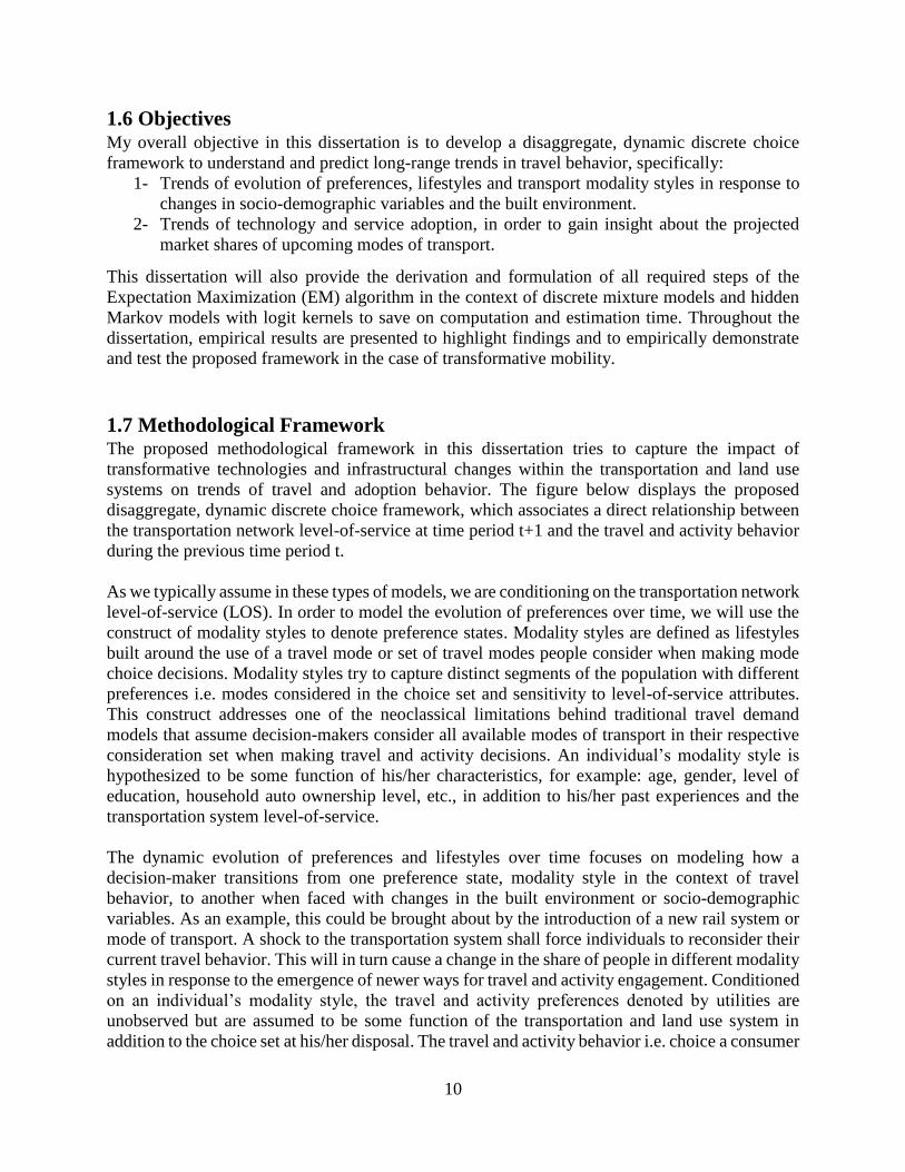
1.7 Methodological Framework The proposed methodological framework in this dissertation tries to capture the impact of

transformative technologies and infrastructural changes within the transportation and land use

systems on trends of travel and adoption behavior. The figure below displays the proposed

disaggregate, dynamic discrete choice framework, which associates a direct relationship between

the transportation network level-of-service at time period t+1 and the travel and activity behavior

during the previous time period t.

As we typically assume in these types of models, we are conditioning on the transportation network

level-of-service (LOS). In order to model the evolution of preferences over time, we will use the

construct of modality styles to denote preference states. Modality styles are defined as lifestyles

built around the use of a travel mode or set of travel modes people consider when making mode

choice decisions. Modality styles try to capture distinct segments of the population with different

preferences i.e. modes considered in the choice set and sensitivity to level-of-service attributes.

This construct addresses one of the neoclassical limitations behind traditional travel demand

models that assume decision-makers consider all available modes of transport in their respective

consideration set when making travel and activity decisions. An individual’s modality style is

hypothesized to be some function of his/her characteristics, for example: age, gender, level of

education, household auto ownership level, etc., in addition to his/her past experiences and the

transportation system level-of-service.

The dynamic evolution of preferences and lifestyles over time focuses on modeling how a

decision-maker transitions from one preference state, modality style in the context of travel

behavior, to another when faced with changes in the built environment or socio-demographic

variables. As an example, this could be brought about by the introduction of a new rail system or

mode of transport. A shock to the transportation system shall force individuals to reconsider their

current travel behavior. This will in turn cause a change in the share of people in different modality

styles in response to the emergence of newer ways for travel and activity engagement. Conditioned

on an individual’s modality style, the travel and activity preferences denoted by utilities are

unobserved but are assumed to be some function of the transportation and land use system in

addition to the choice set at his/her disposal. The travel and activity behavior i.e. choice a consumer

11

Figure 1.5: Proposed Disaggregate, Dynamic Discrete Choice Framework

12

makes comprises the manifestation of those preferences via the Random Utility Maximization

(RUM) principle.

Individual adoption styles on the other hand describe the latent adoption behavior of an individual

to new technologies or services. Similarly, adoption styles are hypothesized to be some function

of the individual’s socio-economic and demographic variables. We are assuming that adoption

styles are not dynamically dependent over time. Adoption styles are innate characteristics of the

decision-maker and will only be influenced by socio-demographic variables.

Now, conditional on both modality styles and adoption styles, the decision to adopt a new

technology or service is some function of the attributes of the innovation and socio-demographic

variables. We are hypothesizing that an individual’s modality style influences the adoption of

newer technologies and services in addition to decisions concerning travel and activity behavior

as mentioned above. The adoption utility at a certain time period is a function of the attributes of

the new technology at that time period. Other explanatory variables can influence the adoption

utility such as social influences whether in the spatial proximity spectrum i.e. an individual’s

neighbors that live in a defined radius away from him/her or in the socio-demographic spectrum

i.e. peers and individuals with similar socio-demographics. Finally, network effect shapes the

adoption behavior in a particular direction. By network effect, we necessitate capturing the

influence of the size of the transportation network to which the new transformative technology can

reach out to. The choice of whether a decision-maker adopts a certain technology or not is observed

and is assumed to be a manifestation of the adoption utility according to RUM principle.

There are three exogenous inputs to the above framework: socio-demographic characteristics of

the population of interest, transportation level-of-service (LOS), and attributes of the new

technology. Changes in socio-demographics, for example an increase in income or auto ownership

levels will influence modality styles and incur changes in travel and activity behavior. Moreover,

these changes will influence adoption styles, which together with changes in modality styles shall

impact adoption behavior. Changes in the transportation system brought about from investments

in infrastructure shall influence modality styles, which will in turn impact travel and activity

behavior. Finally, changes in the attributes of the new technology, will have a direct impact on the

adoption behavior.

1.8 General Overview of Model Framework in This Dissertation The building blocks of the proposed dynamic, disaggregate discrete choice framework are

estimated on two different datasets. First, we will estimate a disaggregate technology adoption

model with a discrete choice kernel. This model tries to understand the technology adoption

process of upcoming modes of transport and project their market shares for certain policies and

investment strategies. Second, we will focus on estimating hidden Markov models with a discrete

choice kernel to model and forecast the evolution of preferences and behaviors over time in

response to changes in socio-demographic variables and the built environment. Together, those

frameworks provide a structural approach to project market shares for various modes of transport

in a more representative manner in the long run.

13

We will build on the following four areas of the literature to address the problem statement of this

dissertation: technology diffusion (both aggregate and disaggregate), travel demand models that

build on the construct of modality styles to capture heterogeneity in the decision-making process,

preference instability in discrete choice models, and dynamic choice models. To develop a

methodological framework to address the first component of our research motivation, we focus on

technology adoption models that employ a microeconomic utility-maximizing representation of

individuals. This framework is of interest to us as it could be integrated with disaggregate activity-

based models. We are also interested in capturing the impact of social influences and network

effect (spatial spectrum) of the new technology on the adoption process. In order to model the

evolution of preferences and lifestyles over time, which is the second component of this

dissertation, we focus on the construct of modality styles (Vij, 2013) to denote preference states.

Finally, dynamic discrete choice models are of interest to us and in particular hidden Markov

models (Baum and Petrie, 1966) as they provide a structural approach to model the evolution of

preferences over time as a function of socio-demographic variables and the built environment.

The first piece of our methodological framework is governed by disaggregate technology adoption

models. We build on the formulation of discrete mixture models and specifically Latent Class

Choice Models (LCCMs), which allow for heterogeneity in the utility of adoption for the various

market segments i.e. innovators/early adopters, imitators and non-adopters. We integrate our

LCCM with a network effect model. The network effect model quantifies the impact of the

spatial/network effect of the new technology on the utility of adoption. We make use of revealed

preference (RP) time series data for a one-way car sharing system in a major city in the United

States. The data entails a complete set of member enrollment ever since the service was launched.

Consistent with the technology diffusion literature, our mixture model identifies three latent

classes (market segments) with utilities of adoption that have a well-defined set of preferences that

are statistically significant and behaviorally consistent. The technology adoption model focuses on

assessing the effects of social influences, network effect, socio-demographics and level-of-service

attributes on the adoption process of an individual. This model is extremely helpful as it allows us

to communicate with each market segment and forecast adoption into the future for several

investment strategies or policies. The model was calibrated and used to forecast adoption for

certain policies and investment strategies. Major findings from the technology adoption model are:

(1) a decision-maker is more likely to be a non-adopter, high-income groups and men are more

likely to be early adopters or innovators; (2) placing a new station/pod for the carsharing system

outside a major technology firm will increase the expected number of monthly adopters the most;

and (3) no significant difference is observed regarding the expected number of monthly adopters

for the downtown region between having a station or on-street parking.

The second piece of the framework focuses on estimating hidden Markov models (HMMs) with

logit kernels to model and predict the evolution of individual preferences, lifestyles and behaviors

over time. The dataset used comes from Santiago, Chile (Yañez, 2010). During February 2007,

the city of Santiago introduced Transantiago, a complete redesign of the public transit system in

the city. The dataset is longitudinal as it entails four one-week pseudo travel diaries throughout a

twenty-two month period that overlapped with the introduction of Transantiago. This dataset offers

the opportunity to investigate the effects of a sudden change in the transportation network and

socio-demographic variables on preferences and lifestyles. We use the construct of modality styles

to denote preference states. It is these modality style preference states that dynamically evolve

14

over time. This dynamic discrete choice model identifies the following modality styles (market

segments) in the population: drivers, bus users, bus-metro users and auto-metro users. The

modality style classes differ in terms of their choice set consideration and their sensitivity to level-

of-service attributes (travel time, travel cost, etc.). The transition probability model identifies how

preferences, which are captured by the construct of modality styles, evolve over time due to

changes in socio-demographic variables and the built environment. Parameter estimates across all

sub-models and in particular the class specific mode choice model were behaviorally consistent

and statistically significant. Indeed, preferences of individuals in the population have shifted over

time in terms of the choice set consideration and sensitivities to level-of-service attributes. This is

denoted by an increase in the share of drivers, auto-metro users, and bus-metro users across the

population after the introduction of Transantiago as opposed to a decrease in the share of bus users.

Finally, a comparison between the proposed dynamic framework and comparable static

frameworks reveals differences in aggregate forecasts for different policy scenarios, demonstrating

the value of the proposed framework for both individual and population-level policy analysis.

1.9 Dissertation Outline The dissertation is organized in the following manner:

Chapter 2 focuses on the formulation and estimation of the disaggregate technology adoption

model. We motivate disaggregate technology adoption models as they could be easily

integrated with activity-based travel demand models. In addition to that, disaggregate models

allow us to quantify the impact of the spatial component of the new technology and its

attributes on the adoption behavior for various types of adopters. We also motivate discrete

mixture models and in particular latent class choice models (LCCMs) that try to capture

unobserved heterogeneity in the decision-making process. The model’s specification tries to

assess the impact of socio-demographics, social influences, network effect (spatial component)

and attributes of the new technology on the adoption behavior. Empirical results are presented

using revealed preference data from a carsharing service in a major city in the United States.

Forecasts of adoption of this new technology are presented for several policies and investment

strategies to highlight the value and importance of the proposed model.

Chapter 3 focuses on the specification and estimation of hidden Markov models (HMMs) with

discrete choice kernels. The proposed methodological framework models and forecasts the

evolution of individual preferences, lifestyles and transport modality styles over time in

response to changes in socio-demographics and the transportation system level-of-service. The

proposed specification of our HMM evaluates how the share of individuals in different

preference states or modality styles will evolve over time, which will in turn impact travel and

activity behavior. This methodological framework will also provide the means to: (1) forecast

trends of travel behavior that are bound to occur as a result of investments in technology and

infrastructure; and (2) predict market shares for modes of transport in the long-run more

accurately.

15

Chapter 4 entails the derivation and formulation of the Expectation Maximization (EM)

algorithm for the two types of models used in this dissertation: discrete mixture models and

hidden Markov models with logit kernels.

Chapter 5 provides a comprehensive summary of the research motivation, objective, adopted

methodological frameworks and corresponding findings. This chapter also focuses on

identifying future research directions for the proposed disaggregate, dynamic discrete choice

framework that caters for transformative technological and infrastructural investments in the

transportation and land use systems.

1.10 Contributions This dissertation focuses on the enhancement of current travel demand models by addressing the

need for demand models for newly-emerging paradigms in travel, such as carsharing and

ridesahring. The proposed methodological framework shall enhance our understanding of the

future of transformative mobility. The proposed quantitative methods shall also improve our

understanding of latent demand in the wake of system improvements where we interpret latent

demand as the unrealized desire for travel that shall occur in the future due to major technological

and infrastructural changes. This dissertation provides the building blocks to advances in travel

demand modeling required to guide transformative mobility to a sustainable and efficient system

via effective policies and investment strategies.

This dissertation makes contributions along three directions. First, the study contributes to the

existing body of literature on technology diffusion through the development of a disaggregate

technology adoption model that caters for the adoption behavior and uptake of new

services/technologies by various market segments. A disaggregate technology adoption model was

developed as it can: (1) be integrated with current activity-based travel demand models; and (2)

account for the spatial/network effect of the new technology to understand and quantify how the

size of the network, governed by the new technology, influences the adoption behavior. Our

technology adoption model accounts for the effects of social influences, network/spatial effect,

socio-demographics and attributes of the technology on the adoption behavior of each of the

market segments. This entails a behaviorally richer dimension as we try to account for taste

heterogeneity in the adoption process for different types of adopters, which will in turn improve

forecasting accuracy. The proposed framework could be used to predict future market shares of

upcoming modes of transport for various policies and investment strategies.

Second, our work contributes to the discrete choice modeling literature by extending the

application of hidden Markov models to model and forecast the evolution of preferences over time

in response to changes in socio-demographics and the built environment. Our framework also

accounts for the influence of past experiences on present preferences. Quantifying the evolution

of preferences is a key ingredient in modeling and predicting trends of travel behavior in response

to transformative technologies and services. Our proposed HMM will enable practitioners and

policy makers to influence and nudge trends of travel behavior to be more sustainable and

multimodal. The proposed dynamic framework shall also improve the accuracy of market share

forecasts in the long-run for various transportation investments and policy decisions.

16

Third, this dissertation tackles a major issue that is bothersome when it comes to estimating

advanced discrete choice models. Advanced models are prone to prolonged computation and

estimation time. In this dissertation, we provide the derivation, formulation, and application of the

Expectation Maximization (EM) algorithm in the context of mixture models and hidden Markov

models with logit kernels. This shall enable travel demand and behavioral modelers to estimate

such advanced models while saving on computation time. Using such a statistical learning

technique i.e. the EM algorithm, model estimation time will be reduced from the order of many

hours to minutes.

17

Chapter 2

A Discrete Choice Framework for Modeling and

Forecasting the Adoption and Diffusion of New

Transportation Services

2.1 Introduction The growth in population and urban development has impacted societies in one way or another

from air pollution to greenhouse gas emission, climate change and traffic congestion. This made

policy makers more inclined towards the development of smart cities that promote sustainable

mobility, connectivity and multimodality. As such, major technological and infrastructural

changes are expected to occur over the next decades such as the introduction of autonomous

vehicles, advances in information and communication technology, California high speed rail,

carsharing and ridesharing. This will induce potential paradigm shifts in the cost, speed, safety,

convenience and reliability of travel. Together, they are expected to influence both short-term

travel and activity decisions, such as where to go and what mode of travel to use, and more long-

term travel and activity decisions, such as where to live and how many cars to own. This

transformative mobility, whether in the form of sharing economy, connected vehicles, autonomous

and app-driven on-demand vehicles and services will revolutionize travel and activity behavior.

Travel demand models are the commonly-used approach by metropolitan planning agencies to

predict 20-30 year forecasts of traffic volumes, transit ridership, walking and biking market shares

across transportation networks. These models try to assess the impacts of transportation

investments, land use and socio-demographic changes on travel behavior with the main objective

of predicting future mode shares, auto ownership levels, etc. These models focus on a behaviorally

richer approach to modeling travel mode choice as opposed to the traditional four step travel

demand models. Travel demand models evaluate travel and activity behavior as a series of

interdependent logit and nested logit models that entail travel mode choice, vehicle availability,

and time-of-day models, etc. However, current travel demand models are unable to predict long-

range trends in travel behavior as they do not entail a mechanism that projects membership and

market share of new modes of transport (Uber, Lyft, autonomous vehicles, etc). According to

Guerra (2015), “only two metropolitan planning organizations in the 25 largest metropolitan areas

mention autonomous or connected vehicles in their long-range regional transportation plans”. That

is why current travel demand models lack a methodological framework that caters for those

upcoming transportation services and technologies and their impact on travel behavior which will

be prevalent in 20-30 years.

Our objective is to develop a methodological framework tailored to model the technology diffusion

process by focusing on quantifying the effect of the spatial configuration of the new technology

and socio-demographic variables. Moreover, we are also interested in capturing the effect of social

influences and level-of-service attributes of the new technology on the adoption process. The

methodological framework used in our analysis entailed an integrated latent class choice model

18

(LCCM) and network effect model that was governed by a destination choice model. Our approach

was confirmatory as the latent classes used in the analysis (innovators/early adopters, imitators

and non-adopters) are rooted in the technology diffusion literature across multiple disciplines.

These latent classes are able to capture heterogeneity in preferences towards technology adoption.

Our research is motivated by existing work in technology adoption modeling which employs a

microeconomic utility-maximizing representation of individuals. This framework is of interest to

us as it could be easily integrated with our disaggregate activity-based models. Our proposed

disaggregate technology adoption model shall help planners and policy makers gain insight

regarding the projected market shares of upcoming modes of transport for various policies and

investment strategies at the public and private levels.

Most diffusion models employ an aggregate framework, for example the Bass model (Bass, 1969).

While recent aggregate models have further enriched the specification of the Bass model, they still

do not account for a range of policy variables (including the spatial configuration) that can be used

to rank policies and investment strategies needed to maximize the expected number of adopters of

a new technology in future time periods. Our methodological framework is different than other

disaggregate models in the diffusion and transportation literature as it accounts for (1)

heterogeneity in the decision-making process across distinct market segments that have a different

adoption behavior; and (2) the spatial configuration effect of the new technology in terms of

quantifying how an increase in the size of the network governed by the new technology will impact

adoption.

This chapter contributes to the existing body of literature in providing a unique methodology to

model the adoption behavior and uptake of new products/technologies by various market

segments. Our model caters for the effects of social influences, network effect, socio-

demographics and level-of-service attributes of the product on the adoption behavior of each of

the market segments. The following framework could be used to predict future market shares of

upcoming modes of transport as one specific type of application. The chapter is organized as

follows: Section 2 provides a literature review of existing technology adoption and diffusion

models. Section 3 provides the adopted methodological framework used to model technology

adoption and details the framework of the dynamic Latent Class Choice Model (LCCM) and the

network effect model. Section 4 explains the dataset used in the study. Section 5 discusses model

results and model applications. Section 6 focuses on comparing forecasts between our proposed

generalized adoption model and the Bass aggregate diffusion model for three different policy

scenarios. Section 7 concludes the findings of this chapter.

19

2.2 Literature Review Autonomous vehicles are on the horizon, not to mention the transformative mobility trend that is

occurring in our transportation system via the introduction of electric vehicles, ridesharing,

carsharing, and many other new technologies. In order to quantify the effect of transportation

policies and investment strategies in a representative manner, travel demand models should be able

to model and forecast market shares for those new modes of transportation. However, current travel

demand models do not entail a mechanism to do so, which in turn provides the core motivation

behind this chapter. We believe that models of technology adoption and diffusion, which are

widely used across multiple industries and cultures to forecast uptake of new technologies, will

bridge this gap in the transportation literature. Diffusion models are popular in a variety of

disciplines such as: agriculture (Sunding and Zilberman, 2001; and Ward & Pulido-Velazquez,

2008), consumer durables (Delre et al., 2007; and Schramm et al., 2010), pharmaceutical industry

(Desiraju et al., 2004), and the automobile industry and in particular aggregate diffusion patterns

of car ownership (Dargay and Gately, 1999). Also, diffusion models have been estimated and used

in forecasting across different cultures such as: United States, France, Spain and many other

countries (please refer to Tellis et al., 2003).

Over the course of the next few paragraphs we will describe the central piece of the framework

governed by the model of technology adoption. The adoption and diffusion of new technologies

have received attention across multiple disciplines within economics and social sciences over the

years. As defined by Rogers (1962), “diffusion is the process by which an innovation is

communicated through certain channels over time among the members of a certain social system”.

Any innovation may be defined in terms of the relative advantage offered by the innovation over

existing alternatives, the degree to which the innovation is consistent with existing needs and

values, the measure of difficulty associated with using the innovation, the extent to which the

innovation can be tried on a limited basis, and the ease with which the benefits of the innovation

are tangible to others. Differences in social systems may be characterized by the pattern of

relationships among members of the system, established norms of what constitutes acceptable and

unacceptable behavior, and the degree to which individual agents are able to influence the behavior

of others. Communication channels can be broadly classified as either mass media, such as the

television, or interpersonal channels that require a direct exchange between two or more

individuals.

Diffusion models are widely used in the marketing science domain and many other industries, as

mentioned above, as they capture the dynamics behind the uptake of a new product in addition to

forecasting its demand. Forecasting accuracy with diffusion models varies depending on the type

of dataset being used, whether it’s homogenous or heterogeneous i.e. from different sources

(Meade and Islam, 2006). Improvement with respect to specification of the diffusion models such

as incorporating non-parametric parametrization and enhancing flexibility has helped increase

forecasting accuracy across multiple disciplines (Meade and Islam, 2006).

Rogers (1962) defines the following five classes of adopters that influence the uptake of a certain

technology across various disciplines: innovators, early adopters, early majority, late majority and

laggards. Based on the mathematical formulation of the diffusion model of Bass (1969), adopters

can be divided into two distinct groups: innovators and imitators with the latter comprising the

remaining four classes of adopters listed above. The technology diffusion literature stresses on the

importance of the role of those two different types of adopters in shaping the market penetration

20

rate of a new good or service (please refer to Mansfield, 1961; Mahajan et al., 1990; and Cavusoglu

et al, 2010). Innovators are individuals that “decide to adopt an innovation independently of the

decisions of other individuals in a social system” while imitators are adopters that “are influenced

in the timing of adoption by the pressures of the social system” (Bass, 1969).

Throughout the next few paragraphs, we will describe the assumptions and formulations of

aggregate and disaggregate technology adoption models, and motivate why disaggregate models

are a better methodological approach to our research question. Aggregate models of technology

diffusion formulate the percentage of the total population that has adopted an innovation at some

time period as some function of the characteristics of the population and the attributes of the

innovation. The empirical research on aggregate models was pioneered by Griliches (1957),

Mansfield (1961), and Bass (1969).The Bass model is well-known in the marketing science

literature and it formulates the probability that a certain consumer will make an initial purchase at

a given time t given that no purchase has been yet made by that specific consumer denoted as 𝑃𝑡

in the equation below as a linear function of the number of previous buyers:

𝑃𝑡 = 𝑝 +𝑞

𝑀Y(t)

𝑝: Coefficient of innovation; 𝑞: Coefficient of imitation; 𝑀: Total potential market for the

technology

Y(t): Cumulative number of individuals that adopted the new technology by time t (number of

previous buyers)

The term 𝑞

𝑀Y(t) reflects the “pressures operating on imitators with an increase in the number of

previous buyers” (Bass, 1969) while 𝑝 reflects the percentage of adopters that are innovators.

Using this formulation, sales of a certain technology/product could be forecasted into the future

via a closed form solution. We are interested in the formulation of the Bass model as it identifies

the two types of adopters of a new technology in addition to capturing the effect of social influence

onto the probability of adoption. The figure below depicts the sales of a product over time (bell-

shaped curve, S(t)) and cumulative sales over time (“S”-shaped curve, Y(t)) according to Bass

(1969). The plot below uses a value of 0.005 for the coefficient of innovation p, 0.3 for coefficient

of imitation q, and 100 for total potential market M. Those values were chosen arbitrarily to display

the shape of the S(t) and Y(t) curves and provide useful insights. It is evident from the “S”-shaped

diffusion curve that once a certain good or service is introduced in a market, it exhibits a low

adoption rate followed by takeoff whereby the market experiences high adoption rates. After the

takeoff period, technology adoption slows down until it reaches market saturation.

Mansfield (1961) on the other hand formulates the cumulative sales of a good/service using a

logistic model, which is a special case of the Bass model (p=0). Extensions of the Bass model and

more recent enhancements to aggregate diffusion models (see for example Kamakura and

Balasubramanian, 1988; and Meade & Islam, 2006), have incorporated the effects of price,

advertising and other marketing variables into the model parametrization in an attempt to increase

forecasting power. Furthermore, aggregate models have been developed to assess the diffusion

levels of a certain technology across different countries. Recently, agent-based modeling and

simulation methods are becoming more popular in the technology diffusion discipline as they are

estimated on an individual level. This will in turn address some of the shortcomings of aggregate

21

diffusion models and cater for heterogeneity among consumers and explicit social structure

(Kiesling et al., 2012; and Schramm et al., 2010).

Figure 2.1: Sales vs. Cumulative Sales over Time

Disaggregate models of technology adoption on the other hand formulate the probability that an

individual or household adopts an innovation as some function of the characteristics of the

decision-maker, attributes of the alternative, communication channels (both interpersonal

networks and mass media) and time in order to cater for the temporal dimension of the diffusion

process. These models have been used to predict the adoption of a wide variety of technologies

and innovations that include color televisions, genetically modified crops, irrigation technology,

computers, diapers and drill bits (Zilberman to al., 2012). Disaggregate models are of interest to

us for the following reasons: (1) they employ a microeconomic utility-maximizing representation

of individuals that provides insight into the decision-making process underlying the adoption or

non-adoption of different innovations by consumers, which is consistent with the framework

typically employed by travel demand models; (2) they capture various sources of heterogeneity in

the decision-making process that will drive different consumers to adopt at different times; (3)

they can be transferable across different geographical, social and cultural contexts with pertinent

model calibration; and (4) they can account for a range of policy variables that can be used to rank

policies and investment strategies in terms of maximizing the expected number of adopters of a

new technology in future time periods. Moreover, we are interested in understanding how the

spatial configuration of a new transportation service and the different socio-demographic variables

of decision-makers can influence the adoption behavior. The aforementioned aggregate models

cannot cater for those two key variables in their formulation to project future market shares of a

0

10

20

30

40

50

60

70

80

90

100

0

1

2

3

4

5

6

7

8

9

0 10 20 30 40 50

Cu

mu

lati

ve S

ales

Sale

s in

Tim

e In

terv

al

Time Period

S(t)

Y(t)

22

new technology in a more representative manner. In addition to that, model application is a key

component in our analysis as it provides policy makers and transportation specialists with the

means to quantify the expected number of adopters for a set of policies and strategies at the

metropolitan levels. Aggregate models do suffer from a limited degree of policy sensitivity and

can only account for a narrow range of policy variables which make them less appealing to our

analysis.

There are various disaggregate diffusion models, each focusing on different aspects of the decision

making process and behavior. One dominant disaggregate adoption model is the threshold model

which was first introduced by David (1969) in an attempt to study the technology adoption of grain

harvesting machinery and was further explored by Sunding and Zilberman (2001). The threshold

model incorporates heterogeneity among decision-makers in the adoption process and could be

used in conjunction with discrete choice models (logit or probit) to represent the utility

maximization behavior of decision-makers. The sources of heterogeneity that affect the adoption

process may include various variables depending on the available data and what the analyst is

trying to capture. At every time period, the critical level of each source of heterogeneity in the

model is determined. Decision-makers equipped with a value of that source of heterogeneity, say

income, that is larger than the critical level at a certain time period will choose to adopt the new

technology/product at that time period. The critical level of a source of heterogeneity shall decrease

over time which induces more consumers to adopt due to principles of “learning by doing” and

“learning by using” (please refer to Sunding and Zilberman, 2001). One application of this

consisted of using a disaggregate utility function model of household vehicle choice using the

threshold model in its aggregate context with income, household structure, and comfort/quality

being three critical sources of heterogeneity (Liu, 2010). Advances in the threshold model

incorporate dynamic optimization in their analysis, such that a decision-maker is making a trade-

off between the expected decrease in price of a certain technology in the future and the current

benefits from purchasing it which will dictate the timing of adoption (McWilliams and Zilberman,

1996).

As we are interested in capturing various sources of heterogeneity in the decision-making process,

the threshold model does not seem to be a good fit to the methodological framework we want to

adopt. As previously mentioned, the literature focuses on two different types of adopters (early

adopters and imitators). We are interested in modeling the adoption behavior of those two distinct

market segments in addition to the non-adopters market segment that chooses to never adopt a new

technology. The formulation of the disaggregate utility function of the threshold model can be

used as a starting point in the development of our methodological framework of technology

adoption for the three different market segments.

What about the transportation industry? The transportation industry has been trying to develop

quantitative methods rooted in the technology diffusion literature to try and predict market shares

of those upcoming modes of transportation. One study (Li et al., 2015), focused on defining

variables that influence ridership of the Taiwan High Speed Rail System (THSR) using

econometric time series models and revealed preference (RP) data of monthly ridership from

January 2007 till December 2013. Two models were estimated: (1) seasonal autoregressive

integrated moving average and (2) first order moving average model to explore the influence of

explanatory variables on ridership.

23

Moreover, studying the market diffusion of electric vehicles has received worldwide attention

these past few years. For example, Plötz et al. (2014), estimated an agent-based simulation model

of the diffusion process of electric vehicles using real-world driving data that captured

heterogeneity among decision-makers, psychological factors and attributes of the new technology.

Another study, please refer to Gnann et al. (2015), used an Alternative Automobiles Diffusion and

Infrastructure (ALADIN) diffusion model to forecast market penetration of plug-in electric

vehicles through simulation techniques. Their proposed methodology incorporated an agent-based

simulation model that catered for different types of users in addition to their respective decision

making processes to make it behaviorally richer. Other studies focused on using agent-based

simulation models alone while others integrated them with discrete choice methods to account for

a richer behavioral interpretation (Eppstein et al., 2011; Brown, 2013; Zhang et al, 2011). For

example in Eppstein et al. (2011), an integrated agent-based and consumer choice model was

estimated that tried to capture the effect of social interactions and media on the market penetration

of plug-in hybrid electric vehicles.

The adoption of new transportation services has primarily focused on using stated preference (SP)

data in the context of alternative fuel vehicles. Some studies were interested in assessing

sensitivities to attributes of the new technology (Ito et al., 2013 and Hirdue et al., 2011) while other

studies focused on both model estimation and forecasting the market share of alternative fuel

vehicles under certain policy scenarios (Glerum et al., 2013, & Mabit and Fosgerau, 2011). The

SP approach does capture sensitivities to attributes of the new technology in a representative way.

However, using SP data does require solid model calibration and validation to enhance the model’s

forecasting power. In order to account for this, integrating SP with revealed preference (RP) data

would be a better approach (see for example Brownstone et al., 2000). Ideally, one should be

interested in using RP data as it represents actual market demand. An SP approach entails

hypothetical scenarios which hinders a model’s forecasting power. In addition to that, the analyst

will not be able to capture the dynamic aspect of the diffusion process over time with respect to

the social influence and spatial component dimensions of the new technology. In previous SP

studies, projected market shares for electric vehicles and alternative fuel vehicles were over

estimated. That is due to the fact that the adoption and diffusion of a new technology is a temporal

and social process and these previous studies did not account for this.

Also, a current developed model focuses on forecasting adoption of electric vehicles using an

integrated discrete choice and diffusion models (Jensen et al., 2016). This model builds on the

previous work of Jun and Park (1999) whereby they specify the utility of adopting a certain good

at time t as a function of the attributes of the technology, and difference between time t and the

time period at which the product was introduced in the market. The parameter associated with the

aforementioned second variable in the utility of adoption will account for the effect of the diffusion

process. The probability of adoption at a certain time period could be computed using the logit

closed form. Following that, the sales of electric vehicles at different time periods could be

computed respectively. To forecast the demand of electric vehicles, data was collected from a

stated preference (SP) survey conducted in Denmark in 2012 and 2013 for the choice between

electric vehicles and internal combustion engines. The specification of the utility of choosing either

mode included purchase price, propulsion costs, driving range, emissions, number of battery

stations, and characteristics of public charging facilities. The utility equation of choosing an

electric vehicle also entailed a parameter that portrays the effect of the diffusion process while

assuming that internal combustion engines have reached market saturation. The model was used

24

to forecast market share of electric vehicles for several policy scenarios. Our proposed

methodological framework is different as it caters for (1) heterogeneity among decision-makers

and in particular among distinct discrete market segments in the population that have different

adoption behavior; (2) effect of various socio-economic and demographic variables on the

diffusion process; (3) spatial or network effect of the new technology whereby we are interested

in assessing how an increase in the size of the network that is covered by the new mode of

transportation will impact adoption behavior; and (4) social influences and how that will influence

the utility of adoption.

2.3 Methodological Framework The methodological framework we want to develop builds on the aggregate diffusion literature

and in particular the concepts of consumer heterogeneity towards the adoption process i.e.

innovators versus imitators, and social influences as described in the Bass model. We are interested

in disaggregate diffusion models as they can be easily integrated with the activity-based travel

demand models of interest. Also, with disaggregate models, we can account for the impact of

socio-demographics and social influences on the adoption process in addition to spatial effects. By

spatial effects we are referring to increasing the relative size of potential destinations that one can

reach out to via the new mode of transport. While there have been disaggregate models developed

in the literature, they seem to be based on different behavioral assumptions (for example the

previously mentioned threshold model) or do not cater for heterogeneity in the specification of the

utility of adoption. Most studies in the literature focus on the role of three defined distinct market

segments in their analysis that differ in their respective adoption behavior towards a new

technology. Those market segments are: innovators/ early adopters, imitators and non-adopters.

We will be building on these findings using a disaggregate technology diffusion approach.

The specification we are interested in developing is unique as it tries to model how technology

adoption and use is influenced by socio-demographics, attributes of the new technology/service,

spatial effect (or network effect) and finally social influences. The aggregate diffusion literature

mainly refers to two types of adopters (innovators and imitators). In order to assess the adoption

behavior of a certain population we need to take into account those decision-makers that will

choose to never adopt the new technology/service. We are interested in modeling the adoption

behavior of each of the following three market segments (innovators/early adopters, imitators, and

non-adopters) to try and capture heterogeneity in the adoption behavior of each of those market

segments. Innovators or early adopters denote the market segment that determines whether a new

technology will pick up in market share or not after being introduced in the market. They define

how steep or flat the “S” cumulative diffusion curve can be during the early stages. Innovators

comprise the biggest fraction of adopters of a new technology during the initial time periods.

Imitators on the other hand come into play as time elapses since the introduction of the new

technology. They will determine the rate at which the market will adopt the new product or service

and will in turn shape the steepness of the “S” cumulative diffusion curve at later stages in the

diffusion process. Non-adopters will define the time period at which the cumulative diffusion

curve reaches a plateau. For example, as the number of non-adopters increases the faster the “S”

curve attains a plateau.

However, we do not observe what type of a person any given individual is i.e. we do not have

information about which market segment each decision-maker belongs to. In order to account for

25

this, discrete mixture models and in particular latent class choice models (LCCM) are found to be

the most appropriate framework. Latent class choice models comprise two components: a class

membership and a class-specific choice model as depicted in the figure below.

The class-specific choice model formulates the probability of technology adoption of a certain

individual conditional on that individual either being an innovator, imitator or non-adopter. This

component captures variation across classes with respect to choice set, tastes and sensitivities,

decision protocol and covariance structure of the error term (Gopinath, 1995).

Figure 2.2: Latent Class Choice Model Framework

As we are interested in modeling the adoption process for each market segment, we should cater

for the temporal dimension of technology diffusion as decision-makers will adopt the new

technology at various time periods according to the aforementioned explanatory variables. Hence,

the probability that individual n during time period t after the new technology was available in the

market adopted or chose to not adopt could be written as:

𝑃(𝑦𝑛𝑡𝑗|𝑍𝑛𝑡 , 𝑋𝑛𝑡𝑗, 𝑞𝑛𝑠) ∀ 𝑗 ∈ {0,1|𝑦𝑛(𝑡−1)𝑗}

where 𝑦𝑛𝑡𝑗 equals one if individual n during time period t chose to adopt the new technology (j=1)

and zero otherwise, conditional on the characteristics of the decision-maker during time period t

denoted as 𝑍𝑛𝑡 and attributes of the new technology (j=1) during time period t denoted as 𝑋𝑛𝑡𝑗,

and conditional on the decision-maker belonging to latent class s (𝑞𝑛𝑠 equals one and zero

otherwise).

Now, evaluating the probability of adoption or non-adoption will be based on a binary logit

formulation that transforms the utility specification into probabilities. Let 𝑈𝑛𝑡𝑗|𝑠 denote the utility

of adoption (j=1) or not (j=0) of the new technology during time period t for individual n

conditional on him/her belonging to latent class s which is expressed as follows:

26

𝑈𝑛𝑡𝑗|𝑠 = 𝑉𝑛𝑡𝑗|𝑠 + 휀𝑛𝑡𝑗|𝑠 = 𝑧𝑛𝑡′ 𝛽𝑠 + 𝑥𝑛𝑡𝑗

′ 𝛾𝑠 + 휀𝑛𝑡𝑗|𝑠

where 𝑉𝑛𝑡𝑗|𝑠 is the systematic utility that is observed by the analyst, 𝑧𝑛𝑡′ is a row vector of

characteristics of the decision-maker n during time period t, 𝑥𝑛𝑡𝑗′ is a row vector of attributes of

the new technology (j=1) during time period t for individual n, 𝛽𝑠 and 𝛾𝑠 are column vectors of

parameters specific to latent class s and 휀𝑛𝑡𝑗|𝑠 is the stochastic component of the utility

specification. Since we have prior assumptions about the behavior of the two various types of

adopters (innovators versus imitators) based on the existing technology diffusion literature, the

systematic utility of adoption for each of the three latent classes was specified according to the

following rationale. The systematic utility of adoption of innovators shall include characteristics

of the decision-maker and attributes of the new technology as we are interested in assessing the

significance of those explanatory variables on the decision process of adopting or not. The

systematic utility of adoption for imitators is also modeled as a function of the characteristics of

the decision-maker and attributes of the new technology. However, this is the latent class whose

adoption behavior is influenced by the extent of social influence and accumulating pressure with

the increase in the previous number of adopters (Bass, 1969). That is why we are interested in

determining the effect of the previous number of adopters on the utility of adoption of imitators at

a certain time period. Finally, the systematic utility of adoption of the third latent class (non-

adopters) consists of an alternative specific constant (ASC) only. Ideally, this ASC should attain a

highly negative value via estimation to ensure that this class will most likely never adopt the new

technology. The systematic utility of adoption / non-adoption for innovators, imitators and non-

adopters is specified in the following manner:

{𝑉𝑎𝑑𝑜𝑝𝑡,𝑛,𝑡|𝑠=𝑖𝑛𝑛𝑜𝑣𝑎𝑡𝑜𝑟 = 𝑧𝑛𝑡

′ 𝛽1 + 𝑥𝑛𝑡𝑗′ 𝛾1

𝑉𝑛𝑜𝑛−𝑎𝑑𝑜𝑝𝑡,𝑛,𝑡|𝑠=𝑖𝑛𝑛𝑜𝑣𝑎𝑡𝑜𝑟 = 0

{𝑉𝑎𝑑𝑜𝑝𝑡,𝑛,𝑡|𝑠=𝑖𝑚𝑖𝑡𝑎𝑡𝑜𝑟 = 𝑧𝑛𝑡

′ 𝛽2 + 𝑥𝑛𝑡𝑗′ 𝛾2 + ∆(𝑡−1)𝛼2

𝑉𝑛𝑜𝑛−𝑎𝑑𝑜𝑝𝑡,𝑛,𝑡|𝑠=𝑖𝑚𝑖𝑡𝑎𝑡𝑜𝑟 = 0

{𝑉𝑎𝑑𝑜𝑝𝑡,𝑛,𝑡|𝑠=𝑛𝑜𝑛−𝑎𝑑𝑜𝑝𝑡𝑒𝑟 = λ

𝑉𝑛𝑜𝑛−𝑎𝑑𝑜𝑝𝑡,𝑛,𝑡|𝑠=𝑛𝑜𝑛−𝑎𝑑𝑜𝑝𝑡𝑒𝑟 = 0

where ∆(𝑡−1) depicts the cumulative number of adopters of the new technology during time period

(t-1), and λ is an alternative specific constant.

Now, in order to assess the impact of the spatial/network effect of the new technology on the utility

of adoption, we were interested in quantifying the level of accessibility brought about by the new

mode of transportation. Accessibility is defined as the “ease with which any land-use activity can

be reached from a location, using a particular transport system” (Dalvi et al., 1976). There are

several types of accessibility measures: cumulative opportunities measures, gravity-based

measures, and utility-based measures (Handy and Niemeier, 1997). We will focus on utility-based

measures for the assessment of accessibility through developing a destination choice zone-based

model. Utility based measures of accessibility have desirable advantages over other methods as

they account for flexibility in travel purposes and sensitivity to travel impedance measures in terms

of time and cost. Also, they capture individual-level preferences and socio-demographic influences

on travel behavior. In those types of models, we assume that given a certain origin, each decision-

maker associates a utility to each of the available destinations in his/her respective choice set 𝐶𝑛

27

and will end up choosing the alternative i.e. destination which maximizes his/her utility.

Accessibility is defined as the logsum measure of those destination choice models as it “measures

the expected worth of certain travel alternatives” (Ben-Akiva and Lerman, 1985).

Let 𝑈𝑛𝑖𝑗 denote the utility of individual n conducting a trip from origin i to destination alternative

j. Determining the systematic utility specification requires assessing the explanatory variables that

influence an individual’s decision to conduct a trip from a certain origin to a certain destination.

Travel impedance whether in terms of travel distance or cost is an important variable as travelers

prefer conducting shorter trips. Second, since travel is a derived demand whereby an individual

goes from a certain origin to a destination to conduct an activity, evaluating the available number

of opportunities or attractions at the destination is important. In addition to that, an individual is

more likely to use the new technology (mode of transport in our case) if it provides a relatively

close destination spot to his/her home. Finally, socio-demographic variables can play a role in

defining some characteristics that can drive individuals into conducting certain trips. Accordingly,

𝑈𝑛𝑖𝑗 was specified in the following manner:

𝑈𝑛𝑖𝑗 = 𝑉𝑛𝑖𝑗 + 휀𝑛𝑖𝑗 = 𝑑𝑖𝑗𝛽 + ln(𝑠𝑖𝑧𝑒𝑗) 𝛼 + 𝑍𝑛𝛾 + 𝑋𝑛𝑗θ + ℎ𝑜𝑚𝑒𝑛𝛿 + 휀𝑛𝑖𝑗

where 𝑉𝑛𝑖𝑗 is the systematic utility observed by the analyst, 𝑑𝑖𝑗 denotes a friction factor of traveling

from origin i to destination alternative j which is the travel distance associated with origin-

destination pair (i,j), 𝑠𝑖𝑧𝑒𝑗 represents the attractions associated with destination j which will be

governed by the employment rate at the destination (number of employees per square mile) as it

is considered to be the driver behind trip attractions, 𝑍𝑛 represents socio-demographic

characteristics of decision-maker n, 𝑋𝑛𝑗 denotes attributes of the new technology at destination

alternative j for individual n, ℎ𝑜𝑚𝑒𝑛 is a dummy variable which will be equal to one if decision-

maker n resides within a certain proximity from his/her corresponding destination alternative and

zero otherwise, 𝛽 , 𝛼, 𝛾, θ, and 𝛿 are parameters associated with the explanatory variables, and 휀𝑛𝑖𝑗

is the stochastic component of the utility specification.

Assuming that all individuals are utility maximizers and that 휀𝑛𝑖𝑗 follows an i.i.d. Extreme Value

Type I distribution across individuals, origin and destination alternatives with mean zero and

variance 𝜋2

6 , the accessibility measure is expressed as the following logsum measure:

𝐴𝑐𝑐𝑒𝑠𝑠𝑖𝑏𝑖𝑙𝑖𝑡𝑦𝑛,𝑖,𝑡 = 𝑙𝑛 [∑ 𝑒𝑉𝑛𝑖𝑗

𝐽𝑡

𝑗=1

]

where i denotes an origin alternative and 𝐽𝑡 is the total number of distinct destination alternatives

available at time period t.

Accessibility changes over time due to an increase/decrease in the number of distinct destination

alternatives 𝐽𝑡 or changes in any of the explanatory variables of the destination choice model

systematic utility. Changes in the employment rate, socio-demographics, or attributes of the new

technology will induce changes in the accessibility measure over time.

Based on the above formulation, the difference in the utility of adoption for the two types of

adopters (early adopters and imitators) comprises different sensitivities to characteristics of the

decision-maker and attributes of the new technology. In addition to that, the adoption process for

28

imitators is affected by the social influence aspect of the new technology while early adopters are

not. Let us focus on a carshring service as an example. Assume a decision-maker resides in a

certain area where the accessibility measure of the new technology is unattractive mainly because

the individual resides in an area that is far away from zones that have a station for this carsharing

service. Also, the nearest station for this service is relatively far from the decision-maker’s home.

In this case, the attributes of the new technology are undesirable, and that individual is unlikely to

adopt. However, as the technology evolves and becomes more attractive, that individual is more

likely to adopt. This decision-maker is an early adopter in his/her local context even though he/she

adopted at a later point in time. Our methodological framework caters for this as it deals with the

micro-level disaggregate decision-making process. Aggregate models on the other hand, such as

the Bass model, examine the diffusion process at a system level whereby they would consider this

particular decision-maker to be an imitator.

Now that we have defined the formulation of the network effect model denoted by accessibility,

we return to the formulation of the class-specific choice model. Assuming that all individuals are

utility maximizers and that 휀𝑛𝑡𝑗|𝑠 follows an i.i.d. Extreme Value Type I distribution across

individuals, time periods, alternatives and latent classes with mean zero and variance 𝜋2

6 , the class-

specific choice model could be formulated as such:

𝑃(𝑦𝑛𝑡𝑗|𝑍𝑛𝑡 , 𝑋𝑛𝑡𝑗, 𝑞𝑛𝑠) = 𝑃(𝑈𝑛𝑡𝑗|𝑠 ≥ 𝑈𝑛𝑡𝑗′|𝑠 ∀ 𝑗′ ∈ 𝐶) = 𝑒

𝑉𝑛𝑡𝑗|𝑠

∑ 𝑒𝑉

𝑛𝑡𝑗′|𝑠𝐽

𝑗′=1

where 𝐶 denotes the choice set i.e. either adopting to the new service or not which is common to

all individuals.

Assuming that the class-specific choice probabilities for individual n across all choice situations

are conditionally independent given that he/she belongs to latent class s, then the conditional

probability of observing a vector of choices 𝑦𝑛 becomes:

𝑃(𝑦𝑛|𝑞𝑛𝑠) = ∏ ∏ 𝑃(𝑦𝑛𝑡𝑗|𝑍𝑛𝑡, 𝑋𝑛𝑡𝑗, 𝑞𝑛𝑠)𝑦𝑛𝑡𝑗

𝑗∈ 𝐶

𝑇𝑛

𝑡=1

where 𝑇𝑛 is the total number of time periods available for individual n until he /she adopts.

The class membership model on the other hand predicts the probability that decision-maker n with

characteristics 𝑍𝑛 belongs to latent class s and is defined as such:

𝑃(𝑞𝑛𝑠|𝑍𝑛)

Let 𝑈𝑛𝑠 denote the utility for individual n from latent class s which is expressed as follows:

𝑈𝑛𝑠 = 𝑉𝑛𝑠 + 휀𝑛𝑠 = 𝑧𝑛′ 𝜏𝑠 + 휀𝑛𝑠

where 𝑉𝑛𝑠 is the systematic utility, 𝑧𝑛′ is a row vector of socio-economic and demographic variables

for decision-maker n, 𝜏𝑠 is a column vector of parameters, and 휀𝑛𝑠 is the stochastic component of

the utility specification. Again, assuming that all individuals are utility maximizers and that 휀𝑛𝑠

follows an i.i.d. Extreme Value Type I distribution across individuals and latent classes with mean

zero and variance 𝜋2

6 , the class membership model could be formulated as such:

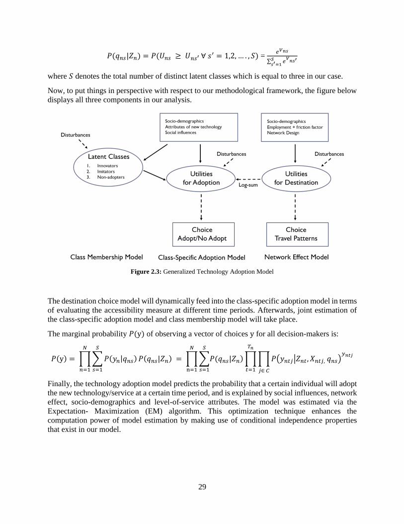
29

𝑃(𝑞𝑛𝑠|𝑍𝑛) = 𝑃(𝑈𝑛𝑠 ≥ 𝑈𝑛𝑠′ ∀ 𝑠′ = 1,2, … . , 𝑆) = 𝑒𝑉𝑛𝑠

∑ 𝑒𝑉

𝑛𝑠′𝑆𝑠′=1

where 𝑆 denotes the total number of distinct latent classes which is equal to three in our case.

Now, to put things in perspective with respect to our methodological framework, the figure below

displays all three components in our analysis.

Figure 2.3: Generalized Technology Adoption Model

The destination choice model will dynamically feed into the class-specific adoption model in terms

of evaluating the accessibility measure at different time periods. Afterwards, joint estimation of

the class-specific adoption model and class membership model will take place.

The marginal probability 𝑃(y) of observing a vector of choices y for all decision-makers is:

𝑃(y) = ∏ ∑ 𝑃(𝑦𝑛|𝑞𝑛𝑠)

𝑆

𝑠=1


𝑁

𝑛=1

= ∏ ∑𝑃(𝑞𝑛𝑠|𝑍𝑛) ∏ ∏ 𝑃(𝑦𝑛𝑡𝑗|𝑍𝑛𝑡 , 𝑋𝑛𝑡𝑗, 𝑞𝑛𝑠)𝑦𝑛𝑡𝑗

𝑗∈ 𝐶

𝑇𝑛

𝑡=1

𝑆

𝑠=1

𝑁

n=1

Finally, the technology adoption model predicts the probability that a certain individual will adopt

the new technology/service at a certain time period, and is explained by social influences, network

effect, socio-demographics and level-of-service attributes. The model was estimated via the

Expectation- Maximization (EM) algorithm. This optimization technique enhances the

computation power of model estimation by making use of conditional independence properties

that exist in our model.

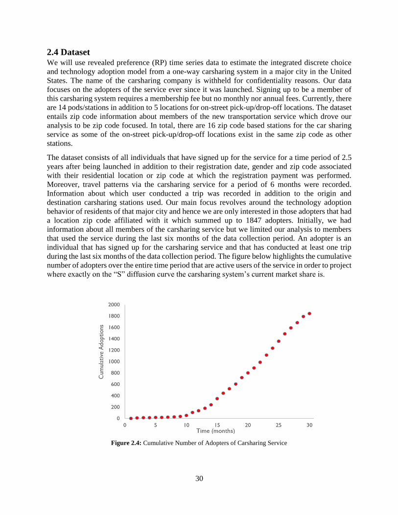
30

2.4 Dataset We will use revealed preference (RP) time series data to estimate the integrated discrete choice

and technology adoption model from a one-way carsharing system in a major city in the United

States. The name of the carsharing company is withheld for confidentiality reasons. Our data

focuses on the adopters of the service ever since it was launched. Signing up to be a member of

this carsharing system requires a membership fee but no monthly nor annual fees. Currently, there

are 14 pods/stations in addition to 5 locations for on-street pick-up/drop-off locations. The dataset

entails zip code information about members of the new transportation service which drove our

analysis to be zip code focused. In total, there are 16 zip code based stations for the car sharing

service as some of the on-street pick-up/drop-off locations exist in the same zip code as other

stations.

The dataset consists of all individuals that have signed up for the service for a time period of 2.5

years after being launched in addition to their registration date, gender and zip code associated

with their residential location or zip code at which the registration payment was performed.

Moreover, travel patterns via the carsharing service for a period of 6 months were recorded.

Information about which user conducted a trip was recorded in addition to the origin and

destination carsharing stations used. Our main focus revolves around the technology adoption

behavior of residents of that major city and hence we are only interested in those adopters that had

a location zip code affiliated with it which summed up to 1847 adopters. Initially, we had

information about all members of the carsharing service but we limited our analysis to members

that used the service during the last six months of the data collection period. An adopter is an

individual that has signed up for the carsharing service and that has conducted at least one trip

during the last six months of the data collection period. The figure below highlights the cumulative

number of adopters over the entire time period that are active users of the service in order to project

where exactly on the “S” diffusion curve the carsharing system’s current market share is.

Figure 2.4: Cumulative Number of Adopters of Carsharing Service

31

Finally, in order to have a representative sample of the population, we wanted to enrich the sample

with a random draw of 2724 observations from the Household Travel Survey (2013) of the same

state to which the city we are working with belongs. We will also assume that the individuals from

this random sample are non-adopters i.e. did not adopt to the new service for the entire data

collection time period (2.5 years). The prior probability of being an adopter in the city of interest

is 3x10-4 given the number of adopters and the population. Hence, the expected number of adopters

in the random sample is approximately one.

The figure below displays the growth in the number of pods/stations and on-street pick-up/drop-

off locations for the 2.5-year time period.

Figure 2.5: Growth in Number of Pods/Stations and On-Street Parking over Time

Our technology adoption model shall assess the impact of socio-demographics, carsharing supply

(fleet and pricing), social influences and network effect on the adoption behavior of innovators,

imitators and non-adopters. Identifying network effect that is governed by the construct of

accessibility shall be restricted to be zip code based for the same reason mentioned above. We

would like to identify the level of accessibility associated with each zip code based station of the

carsharing system depending on the spatial distribution of potential destinations i.e. stations. The

origins and destinations entail the full set of the carsharing system’s stations. The destination

choice model will be estimated based on trips that were conducted by users over a period of 6

months. For our formulation with this dataset, the accessibility measure will be non-zero only for

users that have a home zip code associated with one of the stations or on-street parking locations.

To account for that, we wanted to assign an accessibility measure for zip codes which do not entail

a station/pod or on-street parking. We were interested in imputing the accessibility for those zip

codes from the accessibility of the nearest zip code that had either a station or on-street parking

while taking a friction factor into consideration, distance in our case. The accessibility measure for

individual n with home zip code i which does not have a station or on-street parking at time t could

be defined as follows:

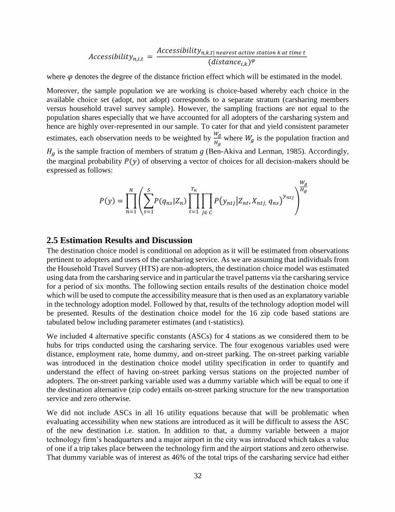
32

𝐴𝑐𝑐𝑒𝑠𝑠𝑖𝑏𝑖𝑙𝑖𝑡𝑦𝑛,𝑖,𝑡 = 𝐴𝑐𝑐𝑒𝑠𝑠𝑖𝑏𝑖𝑙𝑖𝑡𝑦𝑛,𝑘,𝑡| 𝑛𝑒𝑎𝑟𝑒𝑠𝑡 𝑎𝑐𝑡𝑖𝑣𝑒 𝑠𝑡𝑎𝑡𝑖𝑜𝑛 𝑘 𝑎𝑡 𝑡𝑖𝑚𝑒 𝑡

(𝑑𝑖𝑠𝑡𝑎𝑛𝑐𝑒𝑖,𝑘)𝜑

where 𝜑 denotes the degree of the distance friction effect which will be estimated in the model.

Moreover, the sample population we are working is choice-based whereby each choice in the

available choice set (adopt, not adopt) corresponds to a separate stratum (carsharing members

versus household travel survey sample). However, the sampling fractions are not equal to the

population shares especially that we have accounted for all adopters of the carsharing system and

hence are highly over-represented in our sample. To cater for that and yield consistent parameter

estimates, each observation needs to be weighted by 𝑊𝑔

𝐻𝑔 where 𝑊𝑔 is the population fraction and

𝐻𝑔 is the sample fraction of members of stratum g (Ben-Akiva and Lerman, 1985). Accordingly,

the marginal probability 𝑃(𝑦) of observing a vector of choices for all decision-makers should be

expressed as follows:

𝑃(𝑦) = ∏ (∑𝑃(𝑞𝑛𝑠|𝑍𝑛) ∏ ∏ 𝑃(𝑦𝑛𝑡𝑗|𝑍𝑛𝑡 , 𝑋𝑛𝑡𝑗, 𝑞𝑛𝑠)𝑦𝑛𝑡𝑗

𝑗∈ 𝐶

𝑇𝑛

𝑡=1

𝑆

𝑠=1

)

𝑊𝑔

𝐻𝑔𝑁

𝑛=1

2.5 Estimation Results and Discussion The destination choice model is conditional on adoption as it will be estimated from observations

pertinent to adopters and users of the carsharing service. As we are assuming that individuals from

the Household Travel Survey (HTS) are non-adopters, the destination choice model was estimated

using data from the carsharing service and in particular the travel patterns via the carsharing service

for a period of six months. The following section entails results of the destination choice model

which will be used to compute the accessibility measure that is then used as an explanatory variable

in the technology adoption model. Followed by that, results of the technology adoption model will

be presented. Results of the destination choice model for the 16 zip code based stations are

tabulated below including parameter estimates (and t-statistics).

We included 4 alternative specific constants (ASCs) for 4 stations as we considered them to be

hubs for trips conducted using the carsharing service. The four exogenous variables used were

distance, employment rate, home dummy, and on-street parking. The on-street parking variable

was introduced in the destination choice model utility specification in order to quantify and

understand the effect of having on-street parking versus stations on the projected number of

adopters. The on-street parking variable used was a dummy variable which will be equal to one if

the destination alternative (zip code) entails on-street parking structure for the new transportation

service and zero otherwise.

We did not include ASCs in all 16 utility equations because that will be problematic when

evaluating accessibility when new stations are introduced as it will be difficult to assess the ASC

of the new destination i.e. station. In addition to that, a dummy variable between a major

technology firm’s headquarters and a major airport in the city was introduced which takes a value

of one if a trip takes place between the technology firm and the airport stations and zero otherwise.

That dummy variable was of interest as 46% of the total trips of the carsharing service had either

33

that technology firm or airport as an origin or destination. Finally, a dummy variable between the

major technology firm and the city’s downtown region was introduced which takes a value of one

if a trip takes place between the technology firm and downtown, and zero otherwise.

Table 2.1: Destination Choice Model

Variable Parameter Estimate

Distance in 100 Kilometers -0.24 (-2.06)

Employment in Zip Code (employees/miles2) 0.18 (10.06)

Home 1.55 (20.51)

On-street Parking 0.34 (5.47)

Trip between Major Technology Firm and Downtown 1.00 (14.18)

Trip between Major Technology Firm and Major

Airport 2.78 (45.46)

Alternative Specific Constant

Technology Firm

Airport 1

Airport 2

Airport 3

1.10 (13.27)

1.76 (23.07)

0.61 (5.90)

0.93 (10.32)

Using the parameter estimates from the destination choice model, the logsum measure of

accessibility was calculated for all observations in the carsharing service data and the HTS data.

The HTS data does recognize household characteristics but in our case we were only interested in

the following variables: home zip code, gender and work TAZ. Finally, both datasets (HTS and

carsharing service) were integrated together and used to estimate the disaggregate diffusion model.

Since we had apriori hypothesis regarding the number of latent classes in our model, determining

the final model specification was based on varying the utility specification for both sub-models

i.e. class membership and class-specific choice models. The table below presents detailed

parameter estimates (and t-statistics) for the class membership of the technology adoption model.

34

Table 2.2: Class Membership Model

Variable Class 1

Innovators

Class 2

Imitators

Class 3

Non-Adopters

Alternative Specific

Constant -- 7.00 (37.09) 7.51 (56.78)

Monthly Income

($1000) -- -0.23 (-13.01) -0.04 (-3.86)

Male -- -0.77 (-8.70) -1.72 (-23.56)

-- Not applicable

The rho-bar-squared (�̅�2) measure for this technology adoption model is almost 1.0 with a total

number of 4571 individuals and 120,665 observations. �̅�2 has such a high value because of the

weights applied to each of the observations and the fact that the market share of the carsharing

adopters is very minimal compared with the rest of the population, which forces the increase in

model fit.

The class membership model includes parameter estimates which correspond to the influence of

socio-demographic variables on class membership. The class membership model results reveal

that all else equal, an individual is more likely to be a non-adopter, high-income groups and men

are more likely to be early adopters (innovators). The monthly income used in our analysis was

the average zip code based income since that socio-demographic variable was not provided in the

data. Sample enumeration results denote the following split in the population across the three

classes: 0.22% innovators, 16.80% imitators, and 82.98% non-adopters.

The table below presents detailed parameter estimates (and t-statistics) for the class-specific model

corresponding to the adoption behavior of the new technology. Parameter estimates for the utility

of adoption for the two types of adopters have the right sign and are significant at the 1% level

except for the major technology firm employee variable for the innovators latent class. This agrees

with the behavioral interpretation of the adoption process for each class. Early Adopters’ utility of

adoption increases with an individual being an employee of the major technology firm and having

a station or on-street parking for the new transportation service in his/her corresponding zip code.

Also, an increase in the accessibility of a certain home zip code that has neither a station nor on-

street parking will in turn drive an innovator to adopt. A similar behavioral interpretation applies

for home zip codes that do have stations or on-street parking. Imitators’ utility of adoption

increases with an individual being an employee of the major technology firm and with an increase

in the cumulative number of adopters in the previous time period. This is the class which is highly

influenced by previous adopters. Moreover, as the accessibility of the home zip code which has

neither a station nor on-street parking increases, an imitator is more likely to adopt. The same

rationale also applies for home zip codes that do have stations or on-street parking. The behavior

of the non-adopters latent class is deterministic as the probability of non-adoption is almost equal

to one for each individual that belongs to this market segment at each time period.

35

Table 2.3: Class-specific Technology Adoption Model

Variable Parameter Class 1

Innovators

Class 2

Imitators

Class 3

Non-Adopters

Alternative

Specific Constant

(Adoption)

λ -7.88 (-78.08) -14.71 (-78.63) -23.46 (-0.01)*

Major Technology

Firm Employee 𝛽 1.33 (1.89)* 7.10 (46.43) --

Station in Zip

Code

𝛾

1.38 (3.61) -- --

On-street Parking

in Zip Code 1.18 (3.99) -- --

Accessibility for

Zip Codes

Containing a

Station or

On-street Parking

0.44 (5.29) 0.68 (55.39) --

Accessibility for

Zip Codes

Containing neither

a Station nor On-

Street parking

0.91 (22.77) 0.59 (22.64) --

Cumulative

Number of

Adopters at (t-1) in

100’s

𝛼 -- 0.14 (24.21) --

Degree of Distance

Friction Effect for

Accessibility

𝜑 1.00 (--)

-- Not applicable; * Insignificant at the 5% level

36

Finally, the degree of distance friction effect for accessibility, 𝜑, was not directly estimated as our

LCCM evaluates the gradient and standard errors for linear-in-parameter utility equations. In order

to account for this, we estimated several models by varying the value of 𝜑 and selected the value

that maximized the final log-likelihood. This approach is similar to a grid search.

In order to evaluate the performance of our disaggregate adoption model, we will compare its

performance against a multinomial logit (MNL) model. The MNL model comprises two utility

equations: adoption and non-adoption. The adoption utility specification entails all of the

explanatory variables used in the LCCM while the non-adoption systematic utility specification is

constrained to zero. Parameter estimates for the MNL model were behaviorally consistent and

significant. The same dataset that was used to estimate model parameters for the LCCM was used

for the MNL model. The final log-likelihood values for the LCCM and MNL models after

accounting for choice-based sampling were -14.74, and -156.53 respectively. The table below

shows the rho-bar-squared (�̅�2), AIC and BIC values for the two models. It is clear that our

proposed disaggregate adoption model has a slightly higher �̅�2 and lower AIC and BIC values.

That is why it has a better statistical fit as compared with the MNL model. It is interesting to note

that both models have an extremely high �̅�2 value because the marginal probability of adoption in

the population is very small.

Table 2.4: Measures of Model Fit

Model Log-Likelihood �̅�𝟐 AIC BIC

MNL -156.53 0.99 329 407

LCCM -14.74 1.00 65 240

Finally, in order to asses model performance on a hold-out sample, we estimated the parameters

of the disaggregate adoption model using observations for the first 24 months. We calibrated the

model to minimize discrepancy between the predicted number of adopters and the actual number

of adopters for the 25th month. We then used our calibrated model to forecast adoption for months

26-30. We performed simulation using 1000 draws by bootstrapping parameter estimates of the

disaggregate adoption model at each draw. Accordingly we can generate a confidence interval that

bounds the predicted number of adopters. The figure below displays boxplots for the 1000

bootstrap samples in addition to the actual number of adopters for months 26-30.

It is evident that the actual number of adopters for months 27, 28 and 29 fall inside their

corresponding box, which spans the first quartile to the third quartile. As for month 26, the actual

number of adopters falls within the “whiskers”, which is acceptable to a certain extent. This is a

good indication regarding the confidence interval bound of the model’s predicted number of

adopters. That is definitely not the case during the 30th month as the actual number of adopters is

located outside the boxplot’s “whiskers”. It is important to note that a new station for the carsharing

service was introduced at the beginning of the 30th month. However, the actual number of adopters

is much lower than previous months. That could be due to unobserved competition in the market

or some issues in the carsharing service itself, which are not accounted for in our model due to

limitations of the data.

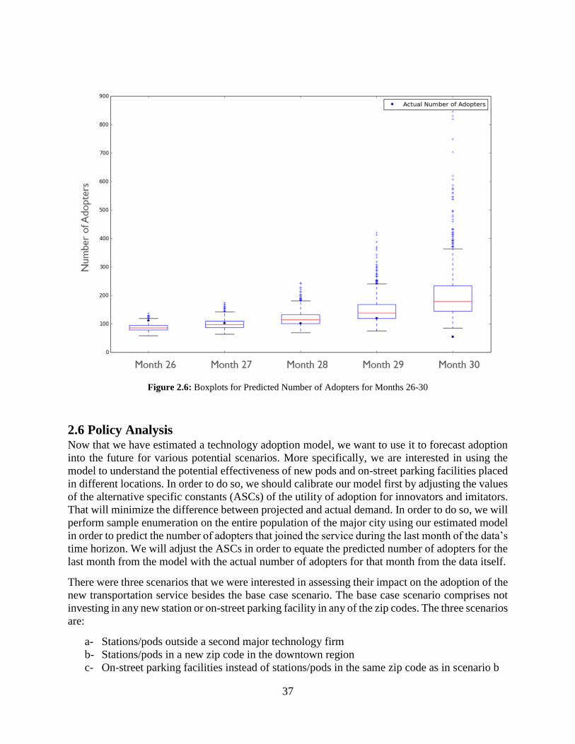
37

Figure 2.6: Boxplots for Predicted Number of Adopters for Months 26-30

2.6 Policy Analysis Now that we have estimated a technology adoption model, we want to use it to forecast adoption

into the future for various potential scenarios. More specifically, we are interested in using the

model to understand the potential effectiveness of new pods and on-street parking facilities placed

in different locations. In order to do so, we should calibrate our model first by adjusting the values

of the alternative specific constants (ASCs) of the utility of adoption for innovators and imitators.

That will minimize the difference between projected and actual demand. In order to do so, we will

perform sample enumeration on the entire population of the major city using our estimated model

in order to predict the number of adopters that joined the service during the last month of the data’s

time horizon. We will adjust the ASCs in order to equate the predicted number of adopters for the

last month from the model with the actual number of adopters for that month from the data itself.

There were three scenarios that we were interested in assessing their impact on the adoption of the

new transportation service besides the base case scenario. The base case scenario comprises not

investing in any new station or on-street parking facility in any of the zip codes. The three scenarios

are:

a- Stations/pods outside a second major technology firm

b- Stations/pods in a new zip code in the downtown region

c- On-street parking facilities instead of stations/pods in the same zip code as in scenario b

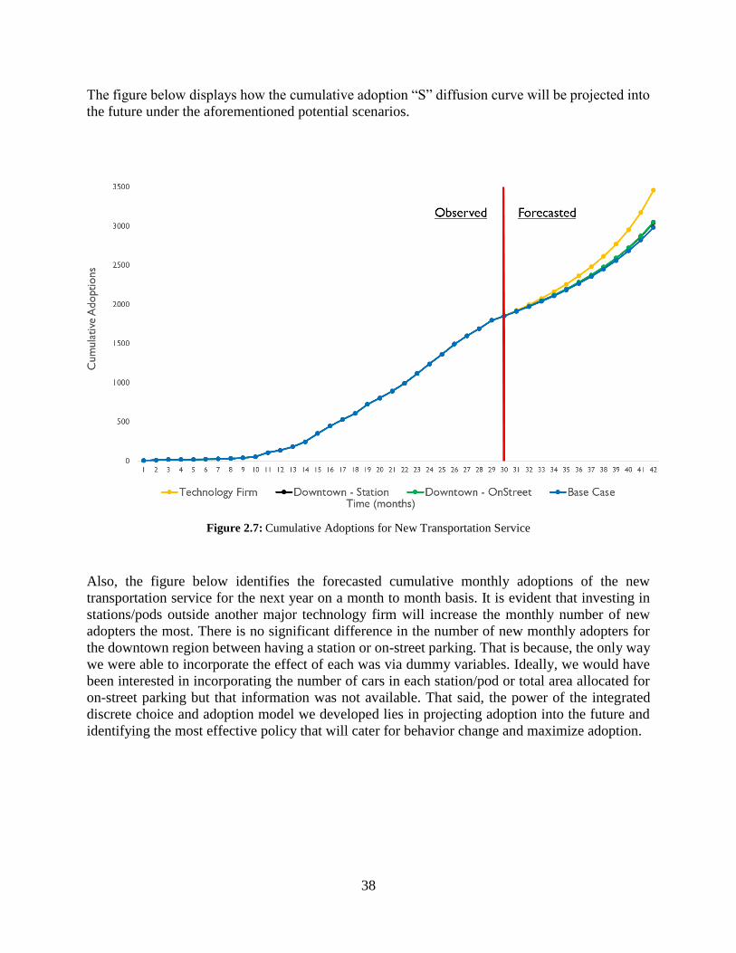
38

The figure below displays how the cumulative adoption “S” diffusion curve will be projected into

the future under the aforementioned potential scenarios.

Figure 2.7: Cumulative Adoptions for New Transportation Service

Also, the figure below identifies the forecasted cumulative monthly adoptions of the new

transportation service for the next year on a month to month basis. It is evident that investing in

stations/pods outside another major technology firm will increase the monthly number of new

adopters the most. There is no significant difference in the number of new monthly adopters for

the downtown region between having a station or on-street parking. That is because, the only way

we were able to incorporate the effect of each was via dummy variables. Ideally, we would have

been interested in incorporating the number of cars in each station/pod or total area allocated for

on-street parking but that information was not available. That said, the power of the integrated

discrete choice and adoption model we developed lies in projecting adoption into the future and

identifying the most effective policy that will cater for behavior change and maximize adoption.

39

Figure 2.8: Forecasted Adoption for New Transportation Service

In order to define confidence intervals for the predicted cumulative number of adopters for each

of the four aforementioned scenarios, we performed simulation using 1000 draws by bootstrapping

estimates of the adoption model at each draw. The figures below display the boxplots for the 1000

bootstrap samples for the predicted cumulative number of adopters for each of the four scenarios.

It is evident that the bound of the confidence interval increases with time. This indicates that

predictions become more stochastic over time, which is a reasonable argument. Again, investing

in stations/pods outside a major technology firm yields the highest number of forecasted adopters.

Moreover, no significant difference is depicted in the predicted cumulative adopters for the

downtown region for an on-street parking facility versus a station/pod.

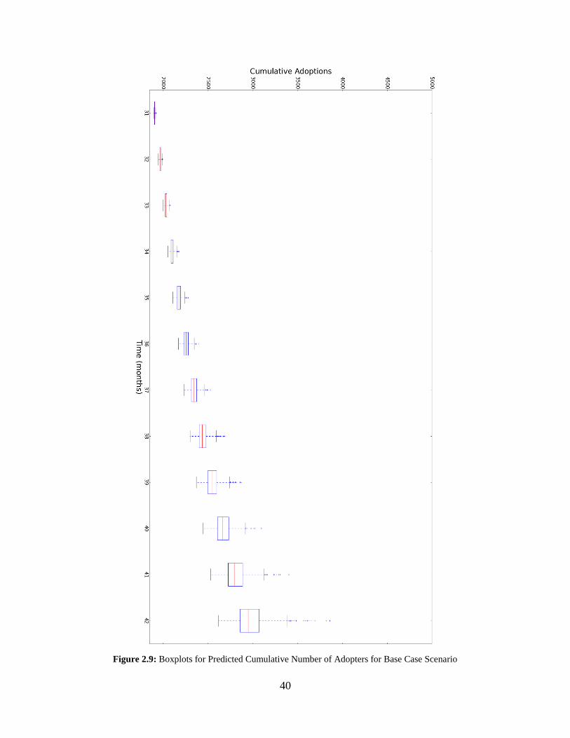
40

Figure 2.9: Boxplots for Predicted Cumulative Number of Adopters for Base Case Scenario

41

Figure 2.10: Boxplots for Predicted Cumulative Number of Adopters for Downtown On-Street Parking Scenario

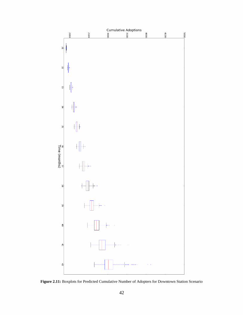
42

Figure 2.11: Boxplots for Predicted Cumulative Number of Adopters for Downtown Station Scenario

43

Figure 2.12: Boxplots for Predicted Cumulative Number of Adopters for Major Technology Firm

44

We were also interested in assessing the aggregate technology adoption process using the Bass

model to highlight the advantages of our adopted methodological framework. The three variables

that need to be calculated which define the “S”-shaped diffusion curve of the cumulative number

of adopters of the one-way carsharing service are: the coefficient of innovation p, for coefficient

of imitation q, and total potential market M. In order to compute the values for those three

variables, we need to define the following formulation (Bass, 1969):

𝑆(𝑡) = 𝑝𝑀 + (𝑞 − 𝑝)𝑌(𝑡) − 𝑞

𝑀𝑌2(𝑡)

S(t) depicts sales of a product over time which is the expected number of adopters of the carsharing

service at time period t. The discrete time series data was used to run the required regression

analysis in order to estimate p, q and M that attained the following values respectively: 0.0051,

0.2108 and 2200. The figure below displays how the number of adopters S(t) and cumulative

number of adopters Y(t) will evolve over time. The cumulative number of adopters will plateau

and attain a value of 2200 adopters. This value is predicted by the Bass model and will disregard

any changes in the attributes of the technology or its spatial configuration that could occur at future

time periods. The Bass model suffers from the following limitations: (1) lack of including

important policy variables into model parametrization which hinders its forecasting power in terms

of identifying effective policies and investment strategies that maximize the expected number of

adopters; (2) absence of key variables that shape the adoption process of a new transportation

service such as the spatial configuration of the service; and (3) absence of incorporating the effect

of socio-demographic variables onto the diffusion process which should be accounted for to

capture heterogeneity in the decision making process across different consumers. That is why, the

Bass diffusion model forecasts displayed below, will be identical across each of the

aforementioned three potential investment strategies / policies.

Figure 2.13: Adopters vs. Cumulative Adopters over Time Using Bass Model

0

500

1000

1500

2000

2500

0

20

40

60

80

100

120

140

0 10 20 30 40 50

Cu

mu

lati

ve S

ales

Sale

s in

Tim

e In

terv

al

Time (months)

S(t)

Y(t)

45

2.7 Conclusion Major technological and infrastructural changes over the next decades, such as the introduction of

autonomous vehicles, implementation of mileage-based fees, carsharing and ridesharing are

expected to have a profound impact on lifestyles and travel behavior. However, the commonly-

used approach for predicting the 20-30 year forecasts across transportation networks suffers from

its inability to project membership of upcoming modes of transport. The methodological

framework used in our analysis to study technology adoption consisted of an integrated latent class

choice model (LCCM) and network effect model that was governed by a destination choice model.

The latent classes used in the analysis are supported by the technology diffusion literature across

multiple disciplines and are defined as: innovators/early adopters, imitators and non-adopters.

These latent classes are able to capture heterogeneity in preferences towards technology adoption.

Each class entails a distinct set of sensitivities and parameter estimates pertinent to the exogenous

variables used in estimation. The adopted methodological framework focuses on understanding

the relative impact of the following set of covariates: social influences, network/spatial effect,

socio-demographics and level-of-service attributes.

One major contribution for this chapter is defining a methodology to capture the impact of the

network/spatial effect of the new technology. We were interested in understanding how the size of

the network, governed by the new mode of transportation, would influence the adoption behavior

of the different market segments as the ability of reaching out to multiple destination increased i.e.

the size of the network grew bigger. This is a critical component in our analysis as it will quantify

the effect of placing stations or on-street parking facilities in different locations and prioritize

locations in the transportation network that will maximize the expected number of adopters. Our

generalized technology adoption model has two other major advantages whereby it employs a

microeconomic utility-maximizing representation of individuals and captures various sources of

heterogeneity in the decision-making process.

The empirical results look promising in terms of defining the adoption behavior of the three

classes. Finally, the model was calibrated and used to project adoption into the future for various

potential scenarios. Some findings from our technology adoption model are: (1) a decision-maker

is more likely to be a non-adopter, high-income groups and men are more likely to be early

adopters or innovators; (2) network/spatial effect, socio-demographics, social influences and level-

of-service attributes of the new technology have a positive set of sensitivities in the utility of

adoption across latent classes which is consistent with our a-priori hypotheses and the diffusion

literature; (3) placing a new station/pod for the carsharing system outside a major technology firm

will increase the expected number of monthly adopters the most; and (4) no significant difference

is observed regarding the expected number of monthly adopters for the downtown region between

having a station or on-street parking.

Acknowledgements We would like to thank UCCONNECT (USDOT and Caltrans) for supporting our research project.

We would also like to thank Susan Shaheen for her assistance in helping us get the data from the

one-way carsharing system. Finally, we would like to show our gratitude to the one-way carsharing

system team that was helpful in answering our questions and concerns.

46

Chapter 3

Modeling and Forecasting the Evolution of

Preferences over Time: A Hidden Markov Model of

Travel Behavior

3.1 Introduction Discrete choice analysts have devoted much attention to the subject of preference heterogeneity.

Preferences, as denoted by taste parameters and consideration sets in the context of utility-

maximizing behavior, are regularly modeled as functions of demographic and situational variables.

For example, value of travel time, or the marginal rate of substitution between travel time and cost

in the context of travel mode choice, is frequently formulated as a function of income, and separate

values of time are usually estimated for work and non-work travel (c.f. Parsons Brinkerhoff Quade

& Douglas, Inc., 2005; Cambridge Systematics, 2002). Recent interest in the influence of latent

psychological, sociological and biological constructs, such as attitudes, normative beliefs and

affective desires, has led to the additional inclusion of these variables within existing

representations of individual preferences (e.g. Bahamonde-Birke, 2015). Some studies have even

contended that preferences are an endogenous function of the decision-making environment, as

characterized by available alternatives and their attributes (e.g. Vij and Walker, 2014). Implicit to

each of these representations is the following assumption: as these explanatory variables change

over time, so should corresponding preferences.

However, most existing frameworks employ static representations of individual behavior that do

not capture preference dependencies over time for the same individual. In addition to the variables

identified previously, an individual’s preferences in the present are expected to be a function of

their preferences in the past, as evidenced by findings across multiple contexts, including

transportation (Carrel et al., 2015), finance (Kaustia and Knüpfer, 2008), health (Gum et al., 2006),

tourism (Sönmez and Graefe, 1998), sustainable development (O’Hara and Stagl, 2002), etc.

Notwithstanding this evidence, discrete choice frameworks that capture such temporal

dependencies are rare in the literature. Part of the limitation is empirical: most studies use cross-

sectional data, and longitudinal data of the kind that is needed is not always available.

The ability to understand and predict how individual preferences evolve over time offers the

potential to address transportation policy questions of great interest. Who is more likely to use

shared mobility services: individuals who currently drive, or those who take public transport? Will

the adoption of driverless cars be led by individuals with significant past exposure to other new

technologies, or individuals with the greatest need for access to self-driving car technology? How

do changes to the public transport system impact individuals that are differently predisposed

towards available travel modes? Transport system use and policy will vary, often considerably,

depending upon the answer to each of these questions. In fact, it is this last question that motivates

the empirical application in this study.

47

The objective of this study is to develop an econometric framework that can model preference

dependencies over time for the same individual. Our proposed framework constitutes a hidden

Markov model (HMM) with a discrete choice kernel. Decision-makers are assumed to be utility-

maximizing, and the unobserved states denote different preferences, as denoted by differences in

taste parameters and consideration sets. Transitions between preferences are expressed as a

function of time-varying covariates, namely socio-demographic variables and alternative

attributes. The evolutionary path is hypothesized to be a first-order Markov process such that an

individual’s preferences during a particular time period are dependent on their preferences during

the previous time period. The framework is empirically evaluated using data from the Santiago

Panel (Yáñez et al., 2010), which comprises four one-week waves of pseudo travel-diary data

spanning a twenty-two month period that extends both before and after the introduction of

Transantiago, a major redesign of the public transport system in Santiago, Chile.

HMMs were first proposed nearly five decades ago (Baum et al., 1970; Baum and Petrie, 1966).

They have a rich history of application in machine learning, with particular regards to the subject

of speech recognition (Rabiner, 1989). They have also been applied, albeit limitedly, to the study

of individual behavior in the applied disciplines of education (e.g. Hong and Ho, 2005; George,

2000), marketing (e.g. Netzer et al., 2008) and transportation (e.g. Xiong et al., 2015; Choudhury

et al., 2010; Goulias, 1999). Our contribution in this chapter is to develop, apply, and test an HMM

framework that captures, models and forecasts the evolution of individual preferences and

behaviors over long-range forecasting horizons.

The remainder of this chapter is organized as follows: Section 2 motivates the study through a

discussion of previous findings on the evolution of individual preferences over time; Section 3

reviews dynamic discrete choice model frameworks that have been used in the past to model

temporal interdependencies in preferences and behavior, and how they relate to our proposed

HMM framework; Section 4 outlines the proposed methodological framework; Section 5 discusses

the initial conditions problem in dynamic discrete choice models, and if and how it applies to

HMMs; Section 6 describes the dataset that constitutes our empirical application; Section 7

presents results from the model framework; Section 8 demonstrates the benefits of the framework

for policy analysis; and finally, Section 9 concludes with a discussion of key findings, limitations

and directions for future research.

48

3.2 Motivation: Evolution of Individual Preferences over Time Most economists would agree that individual preferences, as denoted by taste parameters and

consideration sets in the context of utility-maximizing behavior, can and do change over time.

However, most would also contend that understanding why particular preferences exist in the first

place, and consequently, how they change over time, ought not to be the concern of mainstream

economics. While the view has been challenged over the years (notable examples include Becker,

1996 and Elster, 2016), most contemporary economic representations of individual behavior

continue to treat preferences as exogenously determined, and attention is usually limited to

understanding and predicting policy implications under any given set of preferences.

Preferences may change over time in response to changes in, among others, demographic and

situational variables, psychological, sociological and biological constructs, and available

alternatives and their attributes. Changes in preferences have been observed across a broad

spectrum of behavioral contexts, from the personal to the public. For example, Buss et al. (2001)

examined the evolution of mate preferences between 1939 and 1996 at geographically different

locations in the United States. Their findings indicate that mate preferences did indeed change.

When looking for a potential partner over time, both males and females increased the importance

of physical attraction and financial status, and males decreased the importance of domestic skills.

At the other end of the spectrum, Page and Shapiro (1982) studied the evolution of preferences on

matters of domestic and foreign policy, such as civil liberties, abortion, etc., between 1935 and

1979 in the United States. They found that significant shifts in preferences were rarely the case

over short time periods. However, when opinions and preferences did actually change, that was

the outcome of changes occurring in the decision-making environment, whether in the social and

economic spectrum or in the lives of decision-makers.

In the context of transportation, perhaps the ‘peak car’ phenomenon best represents the notion of

changing preferences over time. The turn of the twenty-first century has witnessed stagnant or

declining levels of car use across much of the developed world (Goodwin and Dender, 2013;

Garceau et al., 2014). The shift in preferences away from the car as a mode of transportation has

been attributed to a combination of economic, social and technological factors that include a

recessionary global economy, fluctuating oil prices, ageing national populations, shifts in cultural

values, advances in information and communications technology, etc. (see, for example, Vij et al.,

2017; McDonald, 2015; Kuhnimhof et al., 2013; Collet, 2012).

What about travel behavior in the era of transformative mobility? Why would one expect

preferences to change over time in response to major changes in the transportation system, such as

the introduction of autonomous vehicles? There may be changes in consideration sets. Individuals

unwilling or unable to drive themselves may be willing and able to use autonomous vehicles. There

may be changes in taste parameters. Being in an autonomous vehicle will allow decision-makers

to multitask, which may cause them to be: (1) less sensitive to driving during peak hours and

getting caught up in congestion; (2) not worried about finding a parking spot in congested cities

nor paying parking fees; and (3) more flexible in terms of residential choice location as they might

consider residing outside dense urban cities and commute via the autonomous vehicle since driving

has become less onerous. These factors may lead to changes in value of time (VOT). The

assumption that preferences are stable may be valid when forecasting over short-term periods.

49

However, when forecasting over long-term horizons, we need to take into account that various

shocks/changes in the built environment and investments in technologies and services are bound

to happen, and that these shocks/changes will likely impact preferences.

Preferences may additionally depend upon past experiences. Though most neoclassical

frameworks assume that preferences are inter-temporally separable, studies on the formation and

persistence of habits have questioned the validity of the assumption (Muellbauer, 1988; von

Weizsäcker, 1971; Pollak, 1970). Past experiences provide a ready yardstick for comparison,

serving both to magnify differences under certain contexts, and reduce contrasts in others. As

Becker (1992) writes, “a given standard of living usually provides less utility to persons who had

grown accustomed to a higher standard in the past. It is the decline in health, rather than simply

poor health, that often makes elderly persons depressed. And what appeared to be a wonderful

view from a newly occupied house may become boring and trite after living there for several

years.”

Past experiences can also serve as anchors, dampening the ability of external events to force

commensurate shifts in individual preferences. Two individuals with completely exchangeable

current circumstances may still differ in terms of their preferences, due to corresponding

differences in their personal histories and the life paths that brought them here. For example,

Bronnenberg et al. (2012), in their study on the long-run evolution of brand preferences among

individual consumers, concluded that “brand capital evolves endogenously as a function of

consumers’ life histories and decays slowly once formed”. Their findings are echoed by studies in

other behavioral contexts. Travel behavior in particular, due to its repetitive nature, is especially

prone to habit formation (Thøgersen, 2006; Gärling and Axhausen, 2003; Sönmez and Graefe,

1998; Aarts et al., 1997). “Habits, once formed, become regularized and the market mechanism

virtually ceases to operate”, and “consequently, if these habits can be identified, choices made at

any future decision point can be predicted with a fairly high degree of accuracy” (Banister, 1978).

As an extreme example, some studies have speculated that the use of active modes of transportation

(i.e. walking and bicycling) as children can promote more sustainable travel behavior practices as

adults (see, for example, Mitra et al., 2010; Faulkner et al., 2009; Roberts, 1996).

However, hypotheses such as these have rarely been tested in the literature, due largely to

limitations on available data. Transportation planning has typically relied on cross-sectional

mobility data for understanding and predicting different dimensions of travel and activity behavior.

Cross-sectional studies can provide population snapshots at a point in time; by extension, repeated

cross-sections can show broad population trends over time. However, cross-sectional studies

cannot measure changes at the level of the individual over time. As mentioned before, the ability

to understand and predict changes in individual-level preferences and behaviors offers the potential

to address transportation policy questions of great interest.

Consider, for example, the peak car phenomenon. A 5% decrease in driving mode shares at the

population level over time could imply that 5% of the population has stopped driving, or that the

entire population is driving 5% less, or some combination of the two (Hanson and Huff, 1988).

The nature and impact of transport policy will depend on which of these competing hypotheses is

true; unfortunately, a traditional cross-sectional study would be unable to distinguish between

these hypotheses. Similarly, consider the case of new transportation technologies and services,

50

such as autonomous and/or alternative-fuel vehicles and shared mobility services, that promise to

transform mobility. The diffusion of new technologies and services is a temporal process (Rogers,

2010). The key to understanding the future of mobility is not only to study the immediate impact

of current policies, services, and nudges; but also how these impacts influence trends and their

evolution over decades, particularly as new technologies and services are introduced. For example,

is the growth in carsharing and ridesharing services being led by individuals who have always been

multimodal, or do these services also appeal to car-dependent households? Will self-driving cars

be subject to the constraints of an ownership-based economy, or will gradual changes in

preferences imply that access and use is facilitated primarily through shared services? Cross-

sectional studies that use static frameworks cannot address these questions. Where such insight is

required, longitudinal studies that use dynamic frameworks are necessary.

3.3 Methodological Basis: Dynamic Models for Discrete Choice Analysis Dynamic discrete choice models try to account for the influence of past experiences on present

choices. According to Kenneth Train (2009), current choices affect future choices, as past choices

affect current choices, and this causality provides the basis for dynamic discrete choice modeling.

There are two broad paradigms in the literature (for an excellent synthesis on the subject, the reader

is referred to von Auer, 1998). Both paradigms assume that present preferences and behavior are

impacted by past experiences; they differ in the ascribed importance of expected future utility on

present behavior.

The first paradigm assumes that individuals, when making a decision at a given time period,

behave as if they are forward-looking agents that maximize their present and expected future

discounted utility over the entire time horizon. Perhaps the most famous example of such a

representation of dynamic discrete choice behavior is the study by Rust (1987) on the optimal

replacement of bus engines. Rust’s representation has since been applied to many contexts,

including car ownership (see for example Cirillo and Xu, 2011; and Glerum et al., 2013), and it is

in this context that we describe the framework. A car is considered a durable good that yields

utility over time. An individual’s choice of whether to purchase a car at a certain time period or

postpone the purchase depends on how that individual expects to use the car both now and in the

future.

The second paradigm assumes a more myopic view of behavior, where individuals are assumed to

maximize their present utility, and future expected utility is completely discounted. In other words,

the individual cares only about the current time period, and choices in later time periods are

deemed irrelevant. For theoretical treatments of such myopic representations of individual

behavior, the reader is referred to, among others, Gorman (1967), Pollak (1970) and von

Weizsäcker (1971). The HMM conforms to this second paradigm, where an individual’s

preferences in the present are assumed to be dependent on their preferences in the past, but at any

given point in time, the individual is assumed only to maximize present utility.

Depending on the empirical context, one or the other paradigm may be preferred. When studying

medium and long-term travel and activity behaviors, such as car ownership and residential

location, it may be more reasonable to assume that individuals are forward-looking. Decisions

51

such as whether to buy a car and where to live have implications that extend well beyond the

present. However, when studying short-term travel and activity behaviors, such as travel mode

choice, it may be more reasonable to assume that individuals are myopic. The impact of these

decisions is typically short-lived and readily reversible. Since our model framework will be applied

to the study of short-term behaviors, we will be adopting a myopic view of decision-making,

articulated through the HMM framework.

As mentioned before, HMMs have been used previously to study the dynamics of travel and

activity behavior. Goulias (1999) used HMMs to study the dynamics of household time allocation

where the dependent variable is continuous. Choudhury et al. (2010) used HMMs to represent the

evolution of latent plans over time, and their consequent impact on actions at any particular point

in time. Their framework does make an explicit link with discrete choice analysis. They apply their

framework to model the “evolution of unobserved driving decisions as drivers enter a freeway.”

Their model is described very generally; extensions such as incorporating the expected maximum

utility are not implemented and applications to long-range modeling and forecasting are not

investigated. Perhaps the empirical application that is closest to the work presented here is the

study by Xiong et al. (2015), who used HMMs to study the dynamic nature of travel mode choice

behavior over time. Their framework does not allow for heterogeneity with regards to

consideration sets, the transition model is not sensitive to changes in available alternatives and

their attributes, and the value of the framework for policy analysis, beyond improvements in fit, is

unclear. Our objective is to build upon these previous studies to develop a methodological

framework capable of modeling the dynamics of preferences over time in a manner that is

theoretically grounded, behaviorally meaningful and practically useful.

52

3.4 Methodological Framework Our methodological framework builds on dynamic models, which are becoming more popular in

the field of travel behavior. For example, Van Acker et al. (2014) highlight the need for

incorporating dynamics into models of behavior by stating that “it will almost inevitably be the

case that the range of travel choices open to people will be wider over time periods in which

lifestyles can also change, than in the short run when the constraints will be more prominent. As

such, the whole way of thinking about travel and lifestyle must be seen as a process of change over

time, not as a fixed state”.

We propose using a hidden Markov model (HMM) with a discrete choice kernel, where the

following two key assumptions are made: (1) we assume a myopic view of behavior, such that

observed choices at a certain time period t are only dependent on corresponding preferences during

that time period, and future expected utility is completely discounted; and (2) the hidden states

denote different preferences, and the evolution of preferences over time is assumed to be a first-

order Markov process such that an individual’s preferences during a certain time period is

dependent on their preferences during the previous time period. Figure 3.1 illustrates the HMM

assumptions. It is important to note that ‘preference state at time 1’ determines the effects of inertia

and past experiences on the probabilistic assignment of each individual to a particular set of

preferences during the first time period.

Figure 3.1: Hidden Markov Model Structure (figure adapted from Choudhury et al., 2010)

Hidden Markov models comprise three components: initialization model, transition model, and

observed output model (Jordan, 2003). The initialization model predicts the probability that a

decision-maker belongs to a certain hidden state during the first time period. The transition model

predicts the probability of observing a certain evolution of hidden states between successive time

periods. Lastly, the observed output model predicts the probability of observing a vector of choices

for a decision-maker at a given time period, conditional on belonging to a certain hidden state

during that time period.

We operationalize the HMM in the context of travel mode choice behavior by relying on the

construct of modality styles. The construct has been introduced in the literature to refer to

overarching lifestyles, built around the use of a particular set of travel modes, that influence all

dimensions of an individual’s travel and activity behavior (Vij et al., 2013). In the context of travel

mode choice behavior, we use modality styles to refer to distinct segments in the population with

53

different travel mode preferences, i.e. modes considered in the choice set, and sensitivity to level-

of-service attributes. For example, modality style models have shown that in 2000, 42% of the San

Francisco Bay Area’s population exclusively considered driving, whereas this share reduced to

23% in 2012 (Vij et al., 2017). Investment in technologies and services are expected to influence

both the travel modes considered and the sensitivity to level-of-service attributes. Consider, for

example, the case of autonomous vehicles. A fully autonomous vehicle that is capable of

navigating itself without human input might prompt changes in the value of time, through its ability

to allow passengers to engage in whatever tasks they wish to while inside the car. Similar changes

in preferences can be imagined in response to other changes in the transportation system. Modeling

what types of modality styles have flourished or declined over time is key to understanding and

predicting mode share shifts in response to policies, services, technologies and nudges.

Accordingly, in the context of travel mode choice behavior, the unobserved states in the dynamic

framework shall be represented by modality styles. Through the remainder of the chapter, we will

use the terms modality styles and (travel mode) preferences interchangeably. The transition model

quantifies the evolution of modality styles over time to capture structural shifts in preferences. Our

dynamic framework requires a transition model that can capture shifts in modality styles brought

about by major changes to the transportation system (sharing, automation, transit on demand) or

by shifts in attitudes (e.g. towards/away from auto-orientation), or changes in socio-demographic

variables.

Figure 3.2: Proposed Dynamic Discrete Choice Framework

Time Period t+1 Time Period t

54

We are interested in forecasting, and thus require a structural model for the transition probabilities

that captures the influence of transportation and societal changes. For this we will employ a

homogenous HMM, which assumes that the transition model between modality styles

(preferences) from one time period to the other is consistent/static i.e. the parameters entering the

transition model between subsequent waves are time-invariant. Any differences in transition

probabilities over waves are assumed to arise due to changes in the explanatory variables entering

the transition model. Figure 3.2 displays the dynamic nature of our framework. Over following

subsections, we explain each of the constituent sub-models in greater detail.

3.4.1 Class-specific Mode Choice Model

The class-specific mode choice model predicts the probability that individual n during time period

t made a set of choices 𝑦𝑛𝑡, conditional on the individual belonging to modality style, or class, 𝑠

during that time period. Note that 𝑦𝑛𝑡 is a vector whose element 𝑦𝑛𝑡𝑘𝑗 equals one if the individual

chose travel mode 𝑗 during choice situation 𝑘 over time period t, and zero otherwise. The model

allows more than one choice situation per individual and time period, and correlation between

these choice situations is captured through the assumption that an individual’s modality style

remains stable over a single time period.

Let 𝑈𝑛𝑡𝑘𝑗|𝑠 denote the utility of travel mode j during choice situation k over time period t for

individual n, conditional on the individual belonging to modality style s, and is expressed as

follows:

𝑈𝑛𝑡𝑘𝑗|𝑠 = 𝑉𝑛𝑡𝑘𝑗|𝑠 + 휀𝑛𝑡𝑘𝑗|𝑠 = 𝑥𝑛𝑡𝑘𝑗′ 𝛽𝑠 + 휀𝑛𝑡𝑘𝑗|𝑠

where 𝑉𝑛𝑡𝑘𝑗|𝑠 is the systematic utility, 𝑥𝑛𝑡𝑘𝑗′ is a row vector of attributes of alternative j during

choice situation k over time period t for individual n, 𝛽𝑠 is a column vector of parameters specific

to modality style s and 휀𝑛𝑡𝑘𝑗|𝑠 is the stochastic component of the utility specification. Now,

assuming that all individuals are utility-maximizers and 휀𝑛𝑡𝑘𝑗|𝑠 follows an i.i.d. Extreme Value

Type I distribution across individuals, time periods, choice situations, alternatives and modality

styles with location zero and scale one, the probability that individual 𝑛 chooses travel mode 𝑗

during choice situation 𝑘 over time period t, conditional on the individual belonging to modality

style 𝑠, is as follows:

𝑃(𝑦𝑛𝑡𝑘𝑗 = 1|𝑞𝑛𝑡𝑠 = 1) = 𝑃(𝑈𝑛𝑡𝑘𝑗|𝑠 ≥ 𝑈𝑛𝑡𝑘𝑗′|𝑠 ∀ 𝑗′ ∈ 𝐶𝑛𝑡𝑘|𝑠) = 𝑒𝑥𝑛𝑡𝑘𝑗

′ 𝛽𝑠

∑ 𝑒𝑥

𝑛𝑡𝑘𝑗′′ 𝛽𝑠

𝑗′∈ 𝐶𝑛𝑡𝑘|𝑠

where 𝑃(𝑦𝑛𝑡𝑘𝑗 = 1|𝑞𝑛𝑡𝑠 = 1) denotes predicting the probability that individual n over wave t and

choice situation k chooses alternative j (implying 𝑦𝑛𝑡𝑘𝑗 equals one and zero otherwise) conditional

on belonging to modality style s during wave t (𝑞𝑛𝑡𝑠 equals one and zero otherwise), and

𝐶𝑛𝑡𝑘|𝑠 denotes the choice set available for individual n at wave t and choice situation k conditional

on modality style s. Preference heterogeneity is captured by allowing both the taste parameters 𝛽𝑠

and the consideration sets 𝐶𝑛𝑡𝑘|𝑠 to vary across modality styles.

55

Assuming that choice probabilities for individual n across all choice situations belonging to time

period t are conditionally independent, given that the individual belongs to modality style s during

time period t, the conditional probability of observing a vector of choices 𝑦𝑛𝑡 for a certain time

period t becomes:

𝑃(𝑦𝑛𝑡|𝑞𝑛𝑡𝑠 = 1) = ∏ ∏ 𝑃(𝑦𝑛𝑡𝑘𝑗 = 1|𝑞𝑛𝑡𝑠 = 1)𝑦𝑛𝑡𝑘𝑗

𝑗∈ 𝐶𝑛𝑡𝑘|𝑠

𝐾𝑛𝑡

𝑘=1

where 𝐾𝑛𝑡 is the number of distinct choice situations observed for individual n over time period

t.

3.4.2 Initialization Model

The initialization model predicts the probability that individual n belongs to modality style s during

the first time period. The probabilities are expressed as a function of individual characteristics

during that time period, denoted by the column vector 𝑧𝑛1. Characteristics may include observable

socio-economic and demographic variables, such as income and gender, or later psychological,

sociological or biological constructs, such as attitudes, normative beliefs or affective desires. In

our case, information on latent constructs was not available across all observation periods, and

characteristics include observable socio-economic and demographic variables only. Depending on

the analyst’s assumption, the model may be formulated as a multinomial logit, multinomial probit,

mixed logit or some other model form. We assume that the initialization model is multinomial

logit.

Let 𝑈𝑛1𝑠 denote the utility of modality style s during the first wave for individual n which is


𝑈𝑛1𝑠 = 𝑉𝑛1𝑠 + 휀𝑛1𝑠 = 𝑧𝑛1′ 𝜏𝑠 + 휀𝑛1𝑠

where 𝑉𝑛1𝑠 is the systematic utility that is observed by the analyst, 𝑧𝑛1′ is a row vector of socio-

economic and demographic variables for individual n during the first wave and 𝜏𝑠 is the associated

column vector of parameter estimates for modality style s, and 휀𝑛1𝑠 is the stochastic component of

the utility specification. Now, assuming that all individuals are utility maximizers and that 휀𝑛1𝑠

follows an i.i.d. Extreme Value Type I distribution across individuals, first wave, and modality

styles with location zero and scale one, the initialization model could be formulated as such:

𝑃(𝑞𝑛1𝑠 = 1|𝑍𝑛1) = 𝑃(𝑈𝑛1𝑠 ≥ 𝑈𝑛1𝑠′ ∀ 𝑠′ = 1,2, … . , 𝑆) =𝑒𝑧𝑛1

′ 𝜏𝑠

∑ 𝑒𝑧𝑛1′ 𝜏𝑠′𝑆

𝑠′=1

where 𝑃(𝑞𝑛1𝑠 = 1|𝑍𝑛1) represents the probability that individual n has modality style s during the

first wave conditional on his/her socio-demographic variables during the first wave, and 𝑆 denotes

the total number of modality styles in the sample.

56

3.4.3 Transition Model

Analogously, the transition model predicts the probability that individual n transitions to modality

style s during time period t, conditional on the individual belonging to modality style r during the

previous time period (t-1). Ordinarily, the probabilities may be expressed as a function only of

individual characteristics during that time period (see, for example, Xiong et al., 2015), as was the

case with the initialization model. Depending on the analyst’s assumption, the transition model

may be formulated as a multinomial logit, multinomial probit, mixed logit or some other model

form. We assume that the transition model is multinomial logit.

Let 𝑈𝑛𝑡𝑠|(𝑡−1)𝑟 denote the utility derived from transitioning into modality style s at wave t

conditional on individual n belonging to modality style r during the previous wave (t-1), which is


𝑈𝑛𝑡𝑠|(𝑡−1)𝑟 = 𝑉𝑛𝑡𝑠|(𝑡−1)𝑟 + 휀𝑛𝑡𝑠|(𝑡−1)𝑟 = 𝑧𝑛𝑡′ 𝛾𝑠𝑟 + 휀𝑛𝑡𝑠|(𝑡−1)𝑟

where 𝑉𝑛𝑡𝑠|(𝑡−1)𝑟 is the systematic utility, 𝑧𝑛𝑡′ is a row vector of observable socio-economic and

demographic characteristics of individual n over wave t and 𝛾𝑠𝑟 is a column vector of parameters

specific to modality style s at wave t given that the individual belonged to modality style r during

wave (t-1), and 휀𝑛𝑡𝑠|(𝑡−1)𝑟 is the stochastic component of the utility specification.

Assuming that all individuals are utility maximizers and that 휀𝑛𝑡𝑠|(𝑡−1)𝑟 follows an i.i.d. Extreme

Value Type I distribution across individuals, waves and modality styles with location zero and

scale one, the transition probability could be formulated as such:

𝑃(𝑞𝑛𝑡𝑠 = 1|𝑞𝑛(𝑡−1)𝑟 = 1) = 𝑃(𝑈𝑛𝑡𝑠|(𝑡−1)𝑟 ≥ 𝑈𝑛𝑡𝑠′|(𝑡−1)𝑟 ∀ 𝑠′ = 1,2, … . , 𝑆) = 𝑒𝑧𝑛𝑡

′ 𝛾𝑠𝑟

∑ 𝑒𝑧𝑛𝑡′ 𝛾𝑠′𝑟𝑆

𝑠′=1

where 𝑃(𝑞𝑛𝑡𝑠 = 1|𝑞𝑛(𝑡−1)𝑟 = 1) denotes one entry of the transition probability matrix, which

involves predicting the probability that individual n belongs to modality style s during wave t, for

t > 1, conditional on modality style r during the previous wave (t-1).

Now, the transition model is merely a function of socio-demographic variables. However,

wouldn’t changes in the level-of-service of the transport network, such as reductions in travel times

or travel costs, influence the transition from one modality style to the other? Changes in the level-

of-service of different travel modes will affect different modality styles differently. For example,

increased freeway congestion will make car-oriented modality styles less attractive, and a

reduction in transit services will have a similar effect on transit-oriented modality styles. These

changes will likely impact whether and how individuals change their modality styles, and should

be accordingly captured by the transition model. We account for these changes by formulating

transition probabilities as an additional function of the consumer surplus each individual would

derive by belonging to different modality styles (building off the static framework forwarded by

Vij and Walker, 2014).

Given that individuals are assumed to be utility-maximizing, the consumer surplus offered by

modality style s to individual n during time period t is given theoretically by the total expected

maximum utility derived by the individual over all observations for that time period, also referred

57

to as the inclusive value. When the class-specific choice model is assumed to be multinomial logit,

expected maximum utility reduces to the familiar logsum measure, and the average consumer

surplus is given by:

𝐶𝑆𝑛𝑡𝑠 =1

𝐾𝑛𝑡∑ 𝑙𝑜𝑔 [ ∑ 𝑒𝑥𝑛𝑡𝑘𝑗

′ 𝛽𝑠

𝑗∈𝐶𝑛𝑡𝑘|𝑠

]

𝐾𝑛𝑡

𝑘=1

The transition probability we are proposing is defined as follows:

𝑃(𝑞𝑛𝑡𝑠 = 1|𝑞𝑛(𝑡−1)𝑟 = 1) =𝑒𝑧𝑛𝑡

′ 𝛾𝑠𝑟+ 𝐶𝑆𝑛𝑡𝛼𝑠𝑟

∑ 𝑒𝑧𝑛𝑡′ 𝛾𝑠′𝑟 + 𝐶𝑆𝑛𝑡𝛼𝑠′𝑟 𝑆

𝑠′=1

where 𝛼𝑠𝑟 is a parameter associated with the consumer surplus specific to modality style s at wave

t given that the individual belongs to modality style r over wave (t-1). For the model to be

consistent with utility-maximizing behavior, 𝛼𝑠𝑟 ≥ 0.

The inclusion of consumer surplus in the transition model provides a basis for understanding and

predicting how individual preferences might change over time in response to corresponding

changes in the transportation system. Consider, for the sake of illustration, that the local public

transport agency introduces a temporary free pass for all services. The introduction of such a pass

would change the consumer surplus offered by different modality styles differently. For modality

styles that do not include public transport in their consideration set, the consumer surplus will be

unchanged. For modality styles that do include public transport, consumer surplus will be higher,

making individuals more likely to belong to these modality styles in the subsequent time period.

In particular, the greatest change will likely be for a modality style that both considers public

transport and is highly sensitive to travel costs (since the free pass will impact travel costs).

Therefore, the introduction of the free pass might not only lead individuals to expand their

consideration sets, it may cause them to become more sensitive to travel costs. Similar changes

could potentially be modeled for other scenarios. This is a key benefit to our framework.

3.4.4 Likelihood Function of the Full Model

Now, the marginal probability 𝑃(𝑦𝑛) of observing a sequence of choices 𝑦𝑛 for decision-maker n

over T time periods is expressed as follows:

𝑃(𝑦𝑛) = ∑ ∑ … ∑ ∏ 𝑃(𝑦𝑛𝑡|𝑞𝑛𝑡𝑠𝑡= 1) 𝑃(𝑞𝑛1𝑠1

= 1|𝑍𝑛1) ∏ 𝑃(𝑞𝑛𝑡𝑠𝑡= 1|𝑞𝑛(𝑡−1)𝑠𝑡−1

= 1)

𝑇

𝑡=2

𝑇

𝑡=1

𝑆

𝑠𝑇=1

𝑆

𝑠2=1

𝑆

𝑠1=1

HMMs are traditionally estimated via the Expectation-Maximization (EM) algorithm (forward-

backward algorithm) that provides a computationally robust method of optimization by taking

advantage of the conditional independence properties of the model framework. The EM algorithm

is particularly useful for HMMs because in the M-step, each of the class-specific choice models,

the initialization model and transition probability model can be maximized independently.

58

However, for HMMs that incorporate feedback to the transition model through the construct of

consumer surplus, that will no longer be the case. The class-specific choice model and the

transition model can no longer be maximized independently in this case, since the class-specific

taste parameters are common to both sub-models. Consequently, the EM algorithm is not useful

in this case, and we resorted to using traditional batch gradient optimization techniques.

3.5 Initialization Problem in Dynamic Models Dynamic models may exhibit what is referred to as the initial conditions problem, first discussed

by Heckman (1981). The initial conditions problem refers to how the dynamic process is

initialized. Heckman (1981) illustrates the problem with the following functional form:

𝑈𝑛𝑡 = 𝑓(𝑥𝑛𝑡, 𝑦𝑛1, 𝑦𝑛2 … 𝑦𝑛(𝑡−1)) + 휀𝑛𝑡

where 𝑈𝑛𝑡 denotes the utility during time period t for individual n, 𝑓 denotes the function that

expresses the observable components of utility, 𝑥𝑛𝑡 entails explanatory variables for time period t

for individual n, 𝑦𝑛(𝑡−1) represents the choice that individual n made during time period (t-1), and

휀𝑛𝑡 is the stochastic error component of the utility specification. We can clearly see that this general

dynamic model captures the effect of previous choices on current ones.

One main assumption in this model formulation entails serially correlated error structure.

According to Heckman (1981), initial conditions can only be treated as exogenous variables if at

least one of the following two conditions is met: (1) serially independent error structures in the

model framework (휀𝑛𝑡) whereby the error components are assumed to be independently and

identically distributed over time; or (2) if the data includes observations since the dynamic process

started. If one of these two conditions is met, then we can treat initial conditions as exogenous

variables or “fixed”. However, if neither of those assumptions is met, then initial conditions cannot

be treated as exogenous variables, and assuming that they are will lead to inconsistent parameter

estimates. The latter condition is almost never going to be met, since the analyst frequently only

observes a dynamic process after it first began. Therefore, in our case, in order to treat the initial

conditions as exogenous, the first condition must hold true.

Heckman (1981) discusses this issue in the context of a fixed effect probit model. Let us reframe

our proposed hidden Markov model using the notation employed by Heckman’s general dynamic

model. The initial conditions problem, in the case of HMMs, is associated with the initialization

model with left-censored datasets. The class-specific choice model could be expressed as follows:

𝑈𝑛𝑡 = 𝑓(𝑥𝑛𝑡, 𝑞𝑛𝑡) + 휀𝑛𝑡

where 𝑥𝑛𝑡 entails explanatory variables for time period t for individual n, 𝑞𝑛𝑡 denotes the modality

style for decision-maker n during time period t.

59

However, according to the aforementioned transition model, one could express the following:

𝑞𝑛𝑡 = 𝑔(𝑧𝑛𝑡, 𝑞𝑛(𝑡−1)) + 𝜏𝑛𝑡

where 𝑔 denotes the function that models the transition of modality styles over time, 𝑧𝑛𝑡 entails

socio-demographic variables for time period t for individual n, and 𝜏𝑛𝑡 is the stochastic error

component. Accordingly, we can express the class-specific choice model utility equation as such:

𝑈𝑛𝑡 = 𝑓′(𝑥𝑛𝑡, 𝑧𝑛𝑡, 𝑞𝑛(𝑡−1)) + 휀𝑛𝑡

We can recursively iterate by replacing the expression of modality styles at different time periods

all the way until the first time period, ending up with the following equation:

𝑈𝑛𝑡 = 𝑓′′(𝑥𝑛𝑡, 𝑧𝑛1 … 𝑧𝑛𝑡) + 휀𝑛𝑡

We are assuming that the choice probabilities that comprise the class-specific choice model for a

certain individual are conditionally independent over choice situations and time periods, given the

modality style they belong to and the set of explanatory variables that affect the choice process.

Thus, the error components in this choice model are independently and identically distributed

across time, i.e. no serial correlation. Therefore, by assuming serially independent error structures,

which is standard in HMMs, initial conditions could be treated as exogenous variables or “fixed”

for the aforementioned reasons.

Conditional on an individual’s modality style, how valid is it to assume that the utilities of different

choice alternatives over time are serially uncorrelated? Factors that lead to serially correlated error

terms entail habit or inertia whereby choices (travel patterns in the case of travel behavior) could

repeat themselves over time (Cantillo et al., 2007; Gärling and Axhausen 2003). The construct of

modality styles tries to capture profound individual variations in preferences and attitudes and

“higher-level orientations, or lifestyles that influence all dimensions of an individual’s travel and

activity behavior” (Vij, 2013). We assume that by conditioning on those higher-level lifestyle

orientations, or modality styles, we are fully accounting for habit or inertia effects.

Another factor behind serial correlation in the case of panel data comprises multiple choice

decisions made by the same individual. This is what we refer to as specification bias, which

encompasses excluding important determinants of choice decisions that are unobserved by the

analyst but are common across multiple choice decisions for the same individual. These

determinants could include unobserved attitudes, missing socio-demographic variables, etc.,

which become confounded with the error terms over time and could induce the main source of

correlation between choice decisions made by the same individual over time. Our hypothesis is

that this shared correlation is captured through the construct of modality styles. That is why, once

we control for those higher-level orientations, it becomes reasonable to assume that choices are

serially independent.

For a hidden Markov model, the evolutionary path, i.e. the transition model, is depicted by a first-

order Markov process, which follows the property:

60

𝜋𝑛 = 𝜋1 ∏ Ω𝑡−1,𝑡

𝑇

𝑡=2

where 𝜋𝑛 denotes the vector of marginal probabilities for the available modality styles at time

period n, 𝜋1 has the same definition as 𝜋𝑛 but is associated with the first time period, and Ω𝑡−1,𝑡

denotes the transition probability matrix between time period (t-1) and t.

If the data is left-censored whereby the time periods which were observed correspond to: {J, J+1,

…, T}, such that J>1, then the initialization model will be biased. Using the above Markov chain

equation, the initialization probabilities evaluated at t=J equal the product of the initialization

probabilities at t=1 and all the transition probabilities up until t=J. In other words, 𝜋𝐽 = 𝜋1 ×

∏ Ω𝑡−1,𝑡𝐽𝑡=2 , and the magnitude of the bias is given by the difference between 𝜋𝐽 and 𝜋1.

However, the transition model and the class-specific choice models will remain unbiased. Our

main objective in this chapter is to develop a framework for modeling and forecasting the

evolutionary path of preferences over time. In order to do so, it is important that parameter

estimates associated with the transition model and class-specific choice model remain unbiased.

Therefore, the initial conditions problem that exists in other types of dynamic models is not of

concern here.

We conducted a Monte Carlo simulation experiment to corroborate our arguments. For our Monte

Carlo simulation, we simulated 5000 observations. Each of the observations entailed 10 time

periods. There were two available states (𝑠1, 𝑠2) that each observation could belong to at each time

period. There were also two available outcomes at each time period. The distribution of the

initialization model, during the first time period, is 0.4 and 0.6 across the two states i.e. 𝜋1 =

[0.4, 0.6]. The transition probability matrix between two successive time periods is Ω𝑡−1,𝑡 =

[0.8 0.20.3 0.7

]. The class-specific choice probabilities were assumed as follows: conditional on being

in the first state, the probability of choosing the first outcome is 0.5, and the probability of choosing

the second outcome is 0.5. However, conditional on being in the second state, the probability of

choosing the first outcome is 0.7, and the probability of choosing the second outcome is 0.3. We

first estimated the hidden Markov model parameters for N=5000 observations over the entire time

periods associated with the dynamic process i.e. T=10. We then re-estimated the HMM parameters

by truncating the dataset by removing the first 5 time periods for each of the 5000 observations.

Table 3.1 summarizes the results from the model estimation using the Expectation –Maximization

algorithm. The initialization model for N=5000 and T=5 could be computed as such: 𝜋6 = 𝜋1 ×

∏ Ω𝑡−1,𝑡6𝑡=2 = [0.59, 0.41]. We can clearly observe that the transition matrix and class-specific

choice models remained unbiased.

61

Table 3.1: Monte Carlo Simulation Results

Variable True Value N = 5000 & T = 10 N= 5000 & T = 5

Initialization Probability (class 1) 0.40 0.39 0.58

Initialization Probability (class 2) 0.60 0.61 0.42

Transition Probability

(class 1 | class 1)

0.80 0.78 0.79


(class 2 | class 1)

0.20 0.22 0.21


(class 1 | class 2)

0.30 0.29 0.29


(class 2 | class 2)

0.70 0.71 0.71

Probability (outcome 1 | class 1) 0.50 0.49 0.49




3.6 Dataset Parts of the following section are adapted from Vij (2013). In February of 2007, Santiago, Chile

introduced Transantiago, a complete redesign of the public transit system in the city. Before the

introduction of Transantiago, public transport in Santiago comprised a privately operated and

uncoordinated system of buses and shared taxis, and the publicly run underground Metro lines.

The old bus system was characterized by a large and inefficient fleet of 8,000 buses operating 380

lines, competition among buses on streets to gain passengers, higher than required frequencies

along the busiest corridors and inadequate service along the less travelled ones, low quality

vehicles, high accident rates, rude drivers, high levels of air and noise pollution, fractured

ownership, and many empty buses circulating during off peak hours (Yáñez et al., 2010). The

Metro system, though considerably safer, faster and more reliable than the bus system, only

accounted for 8% of the city’s trips under the old system, due largely to sparser network coverage

and the high cost of transfers between buses and the Metro.

With the aim of addressing these problems and stemming the decline in the public transportation

system, the city assembled a team of Chilean specialists and consultants in 2005 to come up with

a design for Transantiago (Fernández et al., 2008). Under the new system, the metropolitan region

in and around Santiago was divided into ten zones and operations were taken over by a group of

ten new companies. Bus routes were consolidated into a hierarchical system of trunk and feeder

routes. The feeder routes connected each of these zones to the Metro lines, which served as the

backbone of the new system. The trunk routes complemented the Metro lines by connecting

different zones of the city. Benefits envisaged under Transantiago included the elimination of route

redundancies, increased safety through the introduction of new low-floor buses, approximately

half of them articulated, an integrated fare collection system through the means of a contactless

smart card, lower travel times, a smaller fleet size, and reduced levels of air and noise pollution.

62

Though the system succeeded in achieving many of these goals, as a result of poor implementation

it inadvertently created several new problems. First, the system was introduced in a ‘big-bang’

fashion with no pilot studies or public information campaigns leading up to the change. As a

consequence, the first few weeks following the change resulted in great chaos and confusion

among users of the city’s public transportation system. Second, the system was designed under the

assumption that by the time of its introduction, certain critical bus-only lanes would have been

constructed and all buses in the public transit fleet would have been fitted with on-board GPS

tracking systems. Neither of these goals was achieved in time, and as a consequence buses ran well

below design speeds, introducing significant unreliability into the system. Third, most new bus

routes were confined to run along major arterials, increasing the access and egress distances to bus

stops, particularly in the suburban corners of the city. And finally, given the hierarchical nature of

the new bus system, most bus routes were limited to run within the boundary of a single zone,

increasing the number of transfers for trips that required traversing multiple zones. These four

factors combined drove a number of passengers to alternative modes of travel, most notably the

Metro, which, unlike the bus system, ran at least as reliably as before, resulting in extreme

overcrowding on Metro trains, with average occupancy levels during peak hours on certain routes

of 5-6 passengers per square meter. As one can imagine, Transantiago generated considerable ill

will among city residents, some of which has persisted to this day.

The dataset for the study comes from the Santiago Panel, comprising four one-week waves of

pseudo travel-diary data collected over a span of twenty-two months that extends both before and

after the introduction of Transantiago. The first wave was conducted in December 2006, three

months before Transantiago was introduced, and the next three waves were implemented in May

2007, December 2007 and October 2008, respectively. Survey respondents were drawn from full-

time employees working at one of six campuses of Pontificia Universidad Católica de Chile spread

across Santiago. Each wave of data collection had an observation period of one week, and survey

respondents were asked to report the travel mode(s) that they used for their morning commute to

work each day during that week. Therefore, each wave contains up to five observations per

individual (corresponding to the five-day working week). Though this limits the number of

destinations to just these six campuses, the panel was fortunate in that the distribution of origins

was well spread across the city. In all, the Panel interviewed 303 individuals during the first wave,

286 individuals during the second wave, 279 individuals during the third wave, and 258 individuals

during the final wave. Considering that the four waves were spread across nearly two years, the

Panel has a comparatively low attrition rate. Each of the respondents was asked questions

regarding their socioeconomic characteristics; attributes of their morning trip to work; additional

activities before, during and after work and their influence, if any, on the respondent’s choice of

travel mode; subjective perceptions about the performance of the new system (collected only

during the second and third waves); and their level of agreement with attitudinal statements about

different aspects of the transportation system, such as safety, reliability and accessibility (collected

only during the fourth wave). For more details about the dataset, the reader is referred to Yáñez et

al. (2010).

The dataset offers a unique opportunity to investigate the effects of systemic changes in the

transportation network on the evolution and persistence of individual preferences. For the purpose

of our analysis, we will be restricting our attention to 220 respondents, each of whom has at least

63

one recorded observations in each of the four waves that constitute the Panel. We aggregate the

modal alternatives into seven travel modes: auto, metro, bus, walk, bike, auto/metro (for

individuals that drive to the metro station, and take the metro from there), and bus/metro (for

individuals that take the bus to the metro station, and the metro from there).

Figure 3.3: Mode Shares across All Waves

Figure 3.3 plots mode shares across the four waves for all 220 individuals. It is evident that there

was a big reduction in choosing the bus system as a mode of transport for work trips after wave

one (post introduction of Transantiago). Bus mode shares declined from 40.6% during wave one

to 18.2% during wave three, before marginally rebounding to 21.6% during wave four. Mode

shares for auto/metro and bus/metro increased dramatically after the introduction of Transantiago.

The major shifts in the mode choices occurred between waves one and two, as one would expect.

Shifts tend to stabilize over time as people get more adjusted with their new work trips mode

choice habits.

The reader should note that a plot like figure 3.3 could also have been plotted using repeated cross-

sectional data. Longitudinal data allows us to analyze where these changes in mode shares are

coming from. Figure 3.4 plots the number of trips where individuals switched travel modes

between any two subsequent waves of the Panel. The scale of the vertical axes for each of the three

plots is the same, to make the comparison easier. As one would expect, the majority of the shift

occurs from wave 1 to wave 2, immediately in the wake of the introduction of Transantiago, and

most of it away from “bus” and towards “bus/metro”. However, as the system stabilizes over time,

so does the behavior of its users, with significantly less movement across travel modes between

waves 2 and 3 and waves 3 and 4. Given the nature of the differences between the old and the new

64

system, this is not surprising. The more interesting question is: does the shift in observable travel

mode choice behavior indicate a corresponding shift in latent travel mode preferences? And does

this latter shift, if any, persist beyond the first wave? We address these related questions using the

HMM framework in the next section.

Figure 3.4: Shifts across Travel Modes between Subsequent Waves of the Panel

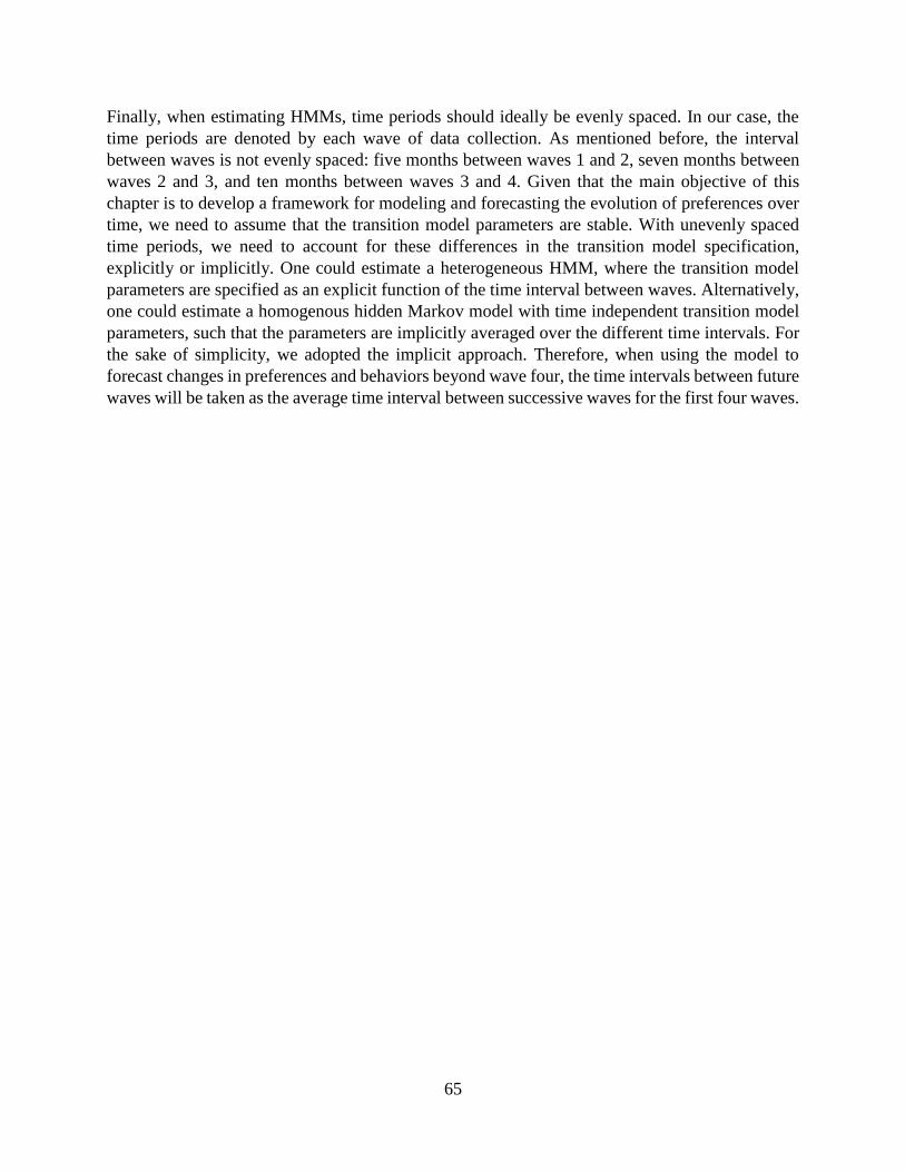
65

Finally, when estimating HMMs, time periods should ideally be evenly spaced. In our case, the

time periods are denoted by each wave of data collection. As mentioned before, the interval

between waves is not evenly spaced: five months between waves 1 and 2, seven months between

waves 2 and 3, and ten months between waves 3 and 4. Given that the main objective of this

chapter is to develop a framework for modeling and forecasting the evolution of preferences over

time, we need to assume that the transition model parameters are stable. With unevenly spaced

time periods, we need to account for these differences in the transition model specification,

explicitly or implicitly. One could estimate a heterogeneous HMM, where the transition model

parameters are specified as an explicit function of the time interval between waves. Alternatively,

one could estimate a homogenous hidden Markov model with time independent transition model

parameters, such that the parameters are implicitly averaged over the different time intervals. For

the sake of simplicity, we adopted the implicit approach. Therefore, when using the model to

forecast changes in preferences and behaviors beyond wave four, the time intervals between future

waves will be taken as the average time interval between successive waves for the first four waves.

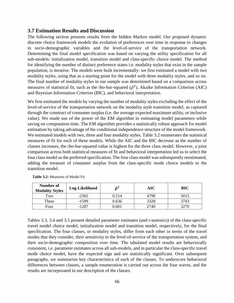
66

3.7 Estimation Results and Discussion The following section presents results from the hidden Markov model. Our proposed dynamic

discrete choice framework models the evolution of preferences over time in response to changes

in socio-demographic variables and the level-of-service of the transportation network.

Determining the final model specification was based on varying the utility specification for all

sub-models: initialization model, transition model and class-specific choice model. The method

for identifying the number of distinct preference states i.e. modality styles that exist in the sample

population, is iterative. The models were built incrementally: we first estimated a model with two

modality styles, using that as a starting point for the model with three modality styles, and so on.

The final number of modality styles in our sample was determined based on a comparison across

measures of statistical fit, such as the rho-bar-squared (�̅�2), Akaike Information Criterion (AIC)

and Bayesian Information Criterion (BIC), and behavioral interpretation.

We first estimated the models by varying the number of modality styles excluding the effect of the

level-of-service of the transportation network on the modality style transition model, as captured

through the construct of consumer surplus (i.e. the average expected maximum utility, or inclusive

value). We made use of the power of the EM algorithm in estimating model parameters while

saving on computation time. The EM algorithm provides a statistically robust approach for model

estimation by taking advantage of the conditional independence structure of the model framework.

We estimated models with two, three and four modality styles. Table 3.2 enumerates the statistical

measures of fit for each of these models. While the AIC and the BIC decrease as the number of

classes increases, the rho-bar-squared value is highest for the three class model. However, a joint

comparison across both statistical measures of fit and behavioral interpretation led us to select the

four class model as the preferred specification. The four class model was subsequently reestimated,

adding the measure of consumer surplus from the class-specific mode choice models to the

transition model.

Table 3.2: Measures of Model Fit

Number of

Modality Styles Log-Likelihood �̅�𝟐 AIC BIC

Two -2365 0.514 4798 5015

Three -1599 0.636 3328 3743

Four -1287 0.601 2740 3270

Tables 3.3, 3.4 and 3.5 present detailed parameter estimates (and t-statistics) of the class-specific

travel model choice model, initialization model and transition model, respectively, for the final

specification. The four classes, or modality styles, differ from each other in terms of the travel

modes that they consider, their sensitivity to the level-of-service of the transportation system, and

their socio-demographic composition over time. The tabulated model results are behaviorally

consistent, i.e. parameter estimates across all sub-models, and in particular the class-specific travel

mode choice model, have the expected sign and are statistically significant. Over subsequent

paragraphs, we summarize key characteristics of each of the classes. To underscore behavioral

differences between classes, a sample enumeration is carried out across the four waves, and the

results are incorporated in our description of the classes.

67

Table 3.3: Class-specific Travel Mode Choice Model Results

Variable Class 1

Drivers

Class 2

Bus Users

Class 3

Bus-Metro Users

Class 4

Auto-Metro Users

Alternative Specific Constant

Auto

Metro

Bus

Walk

Bike

Auto-Metro

Bus-Metro

0.000

(-)

-3.925

(-10.134)

-4.259

(-13.437)

1.935

(6.158)

-0.710

(-3.214)

-3.440

(-11.576)

-3.618

(-9.750)

-

-

0.000

(-)

-

-

-

-

-

0.000

(-)

-7.644

(-19.739)

-

-

-

2.208

(6.965)

0.000

(-)

2.293

(208.455)

-

-

-

4.441

(753.179)

-

Travel Time (mins) -0.028

(-2.968)

-0.042*

(-0.275)

-0.091*

(-0.290)

-0.069

(-3.043)

Walk Time (mins) -0.041

(-3.761)

-0.002*

(-0.019)

-0.127*

(-0.574)

-0.103*

(-0.073)

Travel Cost (CLP) -0.006*

(-1.072)

-0.061*

(-0.280)

-0.102*

(-0.344)

-0.080*

(-0.074)

Waiting Time (mins) -0.024*

(-1.065)

-0.038*

(-0.042)

-0.293*

(-0.790)

-0.053*

(-0.940)

Number of Transfers - -2.633

(-13.894)

-1.136

(-118.488) -

- Not applicable; * Insignificant at the 5% level

Table 3.4: Initialization Model Results

Variable Class 1

Drivers

Class 2

Bus Users

Class 3

Bus-Metro Users

Class 4

Auto-Metro Users

Initialization Model (Wave 1)

Alternative Specific Constant 0.000

(-) 2.993

(5.951)

-0.073*

(-0.160)

0.139*

(0.229)

Household Income

(100,000s CLP)

0.000

(-)

-0.510

(-4.621)

-0.060*

(-1.313)

-0.190

(-2.008)

Male 0.000

(-)

0.223*

(0.521)

0.635*

(1.176)

0.519*

(0.821)

Number of Vehicles 0.000

(-)

-0.992

(-3.159)

-0.739

(-1.979)

-0.295*

(-0.736)


68

Table 3.5: Transition Model Results

Variable Class 1

Drivers

Class 2

Bus Users

Class 3

Bus-Metro Users

Class 4

Auto-Metro Users

Transition Model (Given Class 1 in Wave t- 1)


(-) 0.900

(28.746)

1.351

(12.388)

-2.175

(-44.022)

Household Income

(100,000s CLP)

0.000

(-)

-0.170*

(-0.002)

-0.610*

(-0.010)

-0.080*

(-0.001)

Male 0.000

(-)

0.671

(21.067)

-1.178

(-21.928)

0.359

(21.710)


(-)

-0.385

(-5.752)

-0.416*

(-0.262)

-0.365*

(-0.221)

Consumer Surplus (utils) 0.594*

(0.303)

1.000

(-)

0.264

(43.803) -



(-) 4.833

(7.617)

2.060

(1637.711)

1.223

(382.495)

Household Income

(100,000s CLP)

0.000

(-)

-0.680

(-10.155)

-0.310*

(-0.003)

-0.500*

(-0.005)

Male 0.000

(-)

1.831

(3.014)

1.056*

(1.477)

0.999*

(1.506)


(-)

0.595*

(1.135)

-0.130*

(-0.100)

-0.378*

(-0.248)

Consumer Surplus (utils) 0.330

(110.466)

0.500

(256.703)

0.155*

(0.114)

0.317*

(0.253)



(-) 2.480*

(1.371)

0.936

(414.323)

1.391

(626.478)

Household Income

(100,000s CLP)

0.000

(-)

-1.150

(-2.811)

-0.090*

(-0.001)

-0.930*

(-0.012)

Male 0.000

(-)

0.635*

(0.560)

1.801

(3.300)

-0.641*

(-1.087)


(-)

-1.506*

(-1.495)

-1.143*

(-0.608)

0.184*

(0.143)


(1.688)

0.140*

(0.098)

0.097*

(0.108)

0.364*

(0.560)



(-) 1.064*

(0.504)

0.636

(123.621)

0.968

(1003.253)

Household Income

(100,000s CLP)

0.000

(-)

-0.370*

(-0.712)

-0.060*

(-0.001)

0.050*

(0.001)

Male 0.000

(-)

1.84*

(1.07)

1.03*

(1.10)

0.04*

(0.06)


(-)

-1.805*

(-1.905)

-0.163*

(-0.058)

0.142*

(0.061)


(0.513)

0.094*

(0.501)

0.083*

(0.487) -


69

Class 1 (drivers): This class constitutes 36% of the sample population during wave 1, and the

share of the class slowly but steadily increases to 40% by wave 4. Individuals belonging to this

class consider all available modes of transport, but 70% of all trips are made by auto. Value of

time varies between 0.36$/hr for waiting time and 0.62$/hr for walking time, and the class is

completely insensitive to public transport transfers. High-income men with cars are most likely to

belong to this class.

Class 2 (bus users): This class constitutes 39% of the sample population during wave 1, and the

share of the class steadily decreases to 20% by wave 4. Individuals belonging to this class

deterministically choose bus for all their trips. Value of time is low, at approximately 0.07$/hour

across different travel time components. Note that even though the class-specific choice model is

deterministic, parameters denoting sensitivities to travel times and costs can still be estimated

indirectly through the transition model through the construct of consumer surplus. High-income

individuals with cars are most likely to belong to this class initially, but they are also most likely

to leave this class after the introduction of Transantiago.

Class 3 (bus-metro users): This class constitutes 14% of the sample population during wave 1,

and the share of the class steadily increases to 24% by wave 4. Individuals belonging to this class

consider the metro, bus and bus-metro alternatives. Value of time varies between 0.09$/hr for in-

vehicle time and 0.26$/hr for waiting time. Each public transport transfer is equivalent to 12

minutes of in-vehicle time. Low-income women without access to cars are most likely to belong

to this class.

Class 4 (auto-metro users): This class constitutes 11% of the sample population during wave 1,

and the share of the class increases marginally to 16% by wave 4. Individuals belonging to this

class consider the auto, metro and auto-metro alternatives. Value of time varies between 0.06$/hr

for waiting time and 0.12$/hr for walking time, and the class is completely insensitive to public

transport transfers. While low-income individuals without access to cars are most likely to belong

to this class initially, over time, more high-income individuals with access to cars migrate to this

class.

Now that we have estimated our hidden Markov model, we want to explore the power of this model

in terms of explaining the evolution of preferences, or modality styles, in response to the

introduction of Transantiago. The population distribution of individuals across the four classes for

each of the waves, as determined by sample enumeration, is displayed in figure 3.5. It is evident

that a shock to the transportation network along the lines of Transantiago did force people to

reconsider their modes for travel. The market share of drivers, bus-metro, and auto-metro users

has increased after the introduction of Transantiago, while the market share for bus users has

drastically decreased. These results are aligned with findings from Section 6 regarding mode share

percentages of the different modes across the four waves. We can see that major reductions and

increases in shares of modality styles occurred right after Transantiago revolutionized the public

transit system. These population changes stabilize over time. It is also evident from the figure that

population preferences have in fact changed over time, and in particular after the introduction of

Transantiago.

70

Figure 3.5: Estimated Share of Individuals in Each Modality Style across Waves

However, the stability in preferences at the population level belies the instability at the individual

level. Figure 3.6 illustrates the average transition probabilities between different modality styles

across successive time periods. Note that while figure 3.5 could have been reproduced using a

static framework, such as an LCCM, with repeated cross-sectional data (see, for example, Vij et

al., 2017), figure 3.6 could only be produced using a dynamic framework with longitudinal data,

such as the HMM proposed here. Interestingly, transition probabilities were not found to differ

substantially across time periods, and for this reason, we present average values over all time

periods. There are two key trends to note here. First, construct of habit formation is implicitly

captured in the relative magnitude of the transition probabilities. In general, decision-makers are

more inclined to remain in the same modality style over time than switch to a different modality

style. For three of the four modality styles, the probability of staying in that modality style over

successive time periods is found to be greater than half. And second, there is considerable

instability in travel mode preferences, despite the relative stability at the population level and the

strong influence of habit at the individual level. For example, roughly 30% of bus users and bus-

metro users become drivers each time period. Part of this transition could be explained by the

introduction of Transantiago, which did make use of the public transport system in a more onerous

manner. However, the trend persists beyond wave 2, several months after the introduction of

Transantiago, indicating a more general and ongoing shift in preferences towards the car over time,

triggered possibly in part by the introduction of Transantiago.

0.00

0.05

0.10

0.15

0.20

0.25

0.30

0.35

0.40

0.45

Wave 1 Wave 2 Wave 3 Wave 4

Transit (Bus)

Transit (Bus-Metro)

Transit (Auto-Metro)

Drivers

Fra

ctio

n o

f P

op

ula

tio

n in

Eac

h M

od

alit

y St

yle

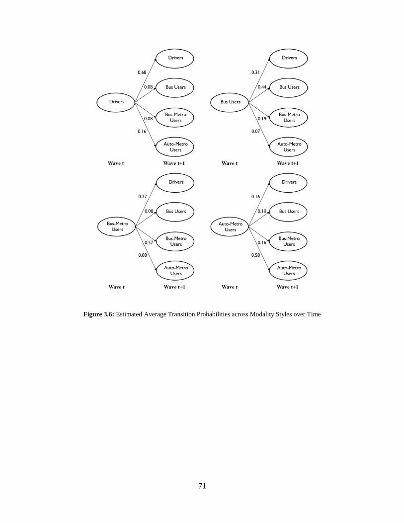
71

Figure 3.6: Estimated Average Transition Probabilities across Modality Styles over Time

72

3.8 Policy Analysis Practitioners and policy analysts are often interested in understanding and predicting broad

population trends in travel and activity behavior. Does failure to account for preference

dependencies over time impact population estimates? Or is it reasonable to ignore such

dependencies when undertaking population-level analysis? We address these questions by

comparing aggregate forecasts from the HMM with static frameworks that do not account for

preference dependencies over time. The forecasting horizon is limited to three waves post the

fourth wave (i.e. waves five, six and seven). We simulate the following two policy scenarios:

1- Increasing household income by 10% at waves five, six and seven respectively.

2- Reducing travel time by 15% for the bus and bus to metro alternatives. This could be

brought about by a new transportation policy, dedicated bus lanes for example. This

particular shock to the transportation network is assumed to take place between waves four

and five.

We compare forecasts from the HMM with latent class choice models (LCCMs). To ensure that

the LCCMs and the HMM are as similar as possible, and any potential differences in forecasts

cannot be attributed to differences in either observed data or model specification, we use the

following procedure. Since an LCCM would typically be estimated using a single cross-section,

we estimate two separate LCCMs using data from the first and last wave respectively. Each of the

LCCMs comprises four modality styles (preference states), same as our HMM. We constrain the

class-specific choice model for each LCCM to be the same as that of the HMM. We only estimate

the class membership model parameters, where we formulate class membership as a function of

socio-demographic variables, namely income, gender and level of car ownership, and the

consumer surplus offered by each class. These are the same variables that are included in the

specification of the transition model for the HMM.

Figure 3.7 plots the change in modality styles across waves five, six and seven for the first policy

scenario, as predicted by the HMM and the two LCCMs, and figure 3.8 plots the corresponding

travel mode shares for the same. As is evident from the figures, even at the population level, there

are considerable differences between forecasts from the three models. In general, the LCCM

estimated using wave 4 data more closely tracks forecasts from the HMM. Relative to the HMM,

the LCCM estimated using wave 4 data under predicts the share of drivers and auto-metro users,

and over predicts the share of bus-metro users, whereas the LCCM estimated using wave 1 data

under predicts the share of bus-metro users, and over predicts the share of drivers and bus users.

These differences translate into similar inconsistencies in travel mode shares. For example, travel

mode shares for the pure public transport modes, i.e. bus, metro and bus to metro, during wave 5

are predicted to be 49% by the HMM, 45% by the LCCM estimated using wave 1 data, and 54%

by the LCCM estimated using wave 4 data.

Figures 3.9 and 3.10 plot corresponding forecasts for the second policy scenario, as predicted by

the HMM and the two LCCMs. Note that the travel mode shares are the same across all three

waves, since the change in the transportation system precedes wave 5. Therefore, we show them

as a single plot.

73

Figure 3.7: Share of Individuals in Each Modality Style for Policy Scenario 1, as Predicted by the HMM, the

LCCM Estimated Using Wave 1 Data, and the LCCM Estimated Using Wave 4 Data

Figure 3.8: Mode Shares for Policy Scenario 1, as Predicted by the HMM, the LCCM Estimated Using Wave 1

Data, and the LCCM Estimated Using Wave 4 Data

74

Figure 3.9: Share of Individuals in Each Modality Style for Policy Scenario 2, as Predicted by the HMM, the

LCCM Estimated Using Wave 1 Data, and the LCCM Estimated Using Wave 4 Data

Figure 3.10: Mode Shares for Policy Scenario 2, as Predicted by the HMM, the LCCM Estimated Using Wave 1

Data, and the LCCM Estimated Using Wave 4 Data

33% 35%31%

10% 10%11%

21%26%

23%

4%

4%

4%2%

2%

2%

11%

11%

9%

18%12%

21%

0%

10%

20%

30%

40%

50%

60%

70%

80%

90%

100%

HMM LCCM Wave 1 LCCM Wave 4

Auto Metro Bus Walk Bike Auto/Metro Bus/Metro

Mo

de

Shar

es (

Per

cen

tage

)

Waves 5, 6, and 7

75

In terms of modality styles, there are considerable differences between forecasts from the three

models, though forecasts from the LCCM estimated using wave 4 data are in closer agreement

with those from the HMM. Interestingly, changes in in-vehicle travel times between waves 4 and

5 do not have a significant impact on the likelihood of belonging to a particular modality style over

subsequent waves, as predicted by each of the three models, and the population distribution

remains largely unchanged across waves 5, 6 and 7. It is important to note that across both

scenarios, the predicted share of drivers and bus users has been strictly higher via the LCCM

estimated using wave 1 data, compared to the other two models, while the share of bus-metro users

has been significantly lower. The reason behind that is the fact that observations pertinent to wave

one (before the introduction of Transantiago) constituted a sample of the population that preferred

taking the bus or driving to work. Moreover, the market share for the metro alternative was

significantly lower during wave one. In addition to that, forecasts from the HMM and LCCM

estimated using wave 4 data seem to be more consistent with each other in terms of the

evolutionary trends of preferences. However, the share of individuals in the four preference states

tends to be different.

In terms of aggregate mode shares, differences across the three models are equally sizeable. For

example, travel mode shares for bus are predicted to be 21% by the HMM, 26% by the LCCM

estimated using wave 1 data, and 23% by the LCCM estimated using wave 4 data. And similarly,

travel mode shares for bus to metro are predicted to be 18% by the HMM, 12% by the LCCM

estimated using wave 1 data, and 21% by the LCCM estimated using wave 4 data. As we argued

before, relative to the HMM, the LCCM estimated using wave 1 data over predicts mode shares

for bus and under predicts mode shares for bus to metro, and the LCCM estimated using wave 4

data over predicts mode shares for bus to metro. These differences are not unexpected. Bus use

was at its greatest during the first wave of observation. And subsequent structural changes in the

public transportation system, initiated by Transantiago, increased the popularity of bus to metro

over the following waves. On one hand, the LCCM estimated using wave 1 data is unable to predict

the full extent of changes in behavior in response to these changes in the transportation system.

On the other, the LCCM estimated using wave 4 data overstates these changes in behavior, as it

does not account for habit formation from preferences and behaviors that precede Transantiago.

3.9 Conclusion The objective of this study was to develop a methodological framework that can model and

forecast the evolution of individual preferences and behaviors over time. Traditionally, discrete

choice models have formulated preferences as a function of demographic and situational variables,

psychological, sociological and biological constructs, and available alternatives and their

attributes. However, the impact of past experiences on present preferences has usually been

overlooked.

We developed a hidden Markov model (HMM) of travel mode choice behavior. The hidden states

denote travel mode preferences, or modality styles, that differ from one another in terms of the

travel modes considered when deciding how to travel, and the relative sensitivity to different level-

of-service attributes of the transportation system. The evolutionary path is assumed to be a first-

order Markov process, such that an individual’s modality style during a particular time period

76

depends only on their modality style in the previous time period. Transitions between modality

styles over time are assumed additionally to depend on changes in demographic variables and the

transportation infrastructure (available travel modes and their attributes). Conditional on the

modality styles that an individual has during a particular time period, the individual is assumed to

choose that travel mode which offers the greatest utility.

The model framework was empirically evaluated using data from the Santiago Panel. The dataset

comprises four waves of one-week pseudo travel diaries each. The first wave was conducted before

the introduction of Transantiago, a complete redesign of the public transit system in Santiago,

Chile, and the next three waves were conducted after. The dataset offered a unique opportunity to

study the impact of a shock to the transportation network on the stability of travel mode preferences

over time. The model identified four modality styles in the sample population: drivers, bus users,

bus-metro users and auto-metro users. At the population level, the proportion of drivers, auto-

metro users, and bus-metro users has increased after the introduction of Transantiago, and the

proportion of bus users has drastically decreased. The biggest shift happens between the first and

second wave, the same period when Transantiago is introduced. The population distribution is

more or less stable across the latter three waves. However, at the individual level, we observe two

interesting phenomena. First, habit formation is found to impact transition probabilities across all

modality styles. Individuals are more likely to stay in the same modality style over successive time

periods than transition to a different modality style. And second, despite both the stability in

preferences at the population level and the influence of habit formation at the individual level,

nearly 40% of the sample population is found to change modality styles between any two

successive waves, reflecting great instability in individual preferences, much after the introduction

of Transantiago. These findings hold implications for aggregate forecasts. We simulated two

policy scenarios using the HMM, and two latent class choice model (LCCM) framework with

comparable specifications, estimated using two separate cross-sections of the Santiago Panel.

Relative to the HMM, the first LCCM, estimated using data from before the introduction of

Transantiago, under predicts changes in travel mode shares, due to its inability to observe the

potential impact of a transformative change such as Transantiago. Relative to the HMM, the

second LCCM, estimated using data from after the introduction of Transantiago, over predicts

changes in travel mode shares, due to its inability to account for habit formation of preferences

and behaviors from before the introduction of Transantiago.

There are two key directions in which future research can build on findings from this study. First,

the methodological framework developed here captures preference dependencies across time for

the same individual, explicitly accounting for the effect of habit formation on travel behavior. The

framework offers the potential to improve the accuracy of the long-range forecasts made from

large-scale urban travel demand models. Future research should explore ways in which existing

travel demand modeling paradigms can adopt dynamic representations of behavior that capture

temporal trends in preferences and behaviors. And second, the framework developed here provides

a quantitative basis for modeling and forecasting structural shifts in preferences that are bound to

occur in this era of transformative mobility. We observed great flux in individual commute travel

mode preferences over time, triggered at least in part by a major redesign of the public

transportation system. It would be interesting to see how these findings compare with

corresponding changes in preferences across other dimensions of travel behavior, such as car

77

ownership and residential location, and in response to other changes in transport policy,

infrastructure and services, such as the introduction of congestion charge schemes, the diffusion

of alternative-fuel vehicles and the emergence of shared mobility services.

Acknowledgements We would like to thank Juan de Dios Ortúzar for providing us access to the Santiago panel, which

was used to estimate our dynamic choice model; and Tony Marley, for very thoughtful and detailed

feedback on an earlier draft of this chapter.

78

Chapter 4

Expectation Maximization Algorithm: Derivation and

Formulation for Mixture Models and Hidden Markov

Models with Logit Kernels

4.1 Introduction Statistical inference for mixture models and hidden Markov models could be conducted using

traditional batch gradient descent algorithms to maximize the likelihood function. However, due

to the non-convex nature of the objective function, direct maximization of the likelihood could

become difficult and highly unstable. Traditional optimization methods, for example Newton

Raphson, have the following limitations: (1) evaluating the gradient (set of first derivatives)

becomes more complicated and requires significantly more time with an increase in the number of

parameters; and (2) inversion of the hessian becomes numerically more difficult with the

possibility of empirical singularity at some iterations (Train, 2008). Those issues are likely to occur

as the number of parameters to be estimated increases and as maximizing the likelihood function

becomes more complex and numerically difficult, which is the case with advanced discrete choice

models that entail latent variables.

The EM algorithm, first introduced by Dempster et al. (1977), is a statistical learning technique

used in models that entail discrete latent variables and use the method of maximum likelihood to

estimate parameters (Jordan, 2003). The EM algorithm provides a more efficient approach to deal

with the above issues by maximizing a lower bound function of the maximum likelihood (an

expectation function), which is computationally much easier to maximize as opposed to the

model’s full likelihood function (Train, 2008). The EM algorithm framework comprises the

following three steps: (1) writing the complete log-likelihood function assuming the discrete latent

variables are in fact observed; (2) evaluating the expectation of all required sufficient statistics

conditioned on the observed variables and current estimates of the unknown parameters denoted

as the E-step; and (3) maximizing the complete log-likelihood function to update parameter

estimates conditioned on the observed variables and expectation of the sufficient statistics denoted

as the M-step. The algorithm alternates between the E-step and M-step until the convergence

criterion is met. The EM algorithm tends to be more stable than gradient-descent based algorithms

when latent variables are involved, and requires fewer iterations to converge by taking advantage

of the conditional independence structure of the model framework. As we will see in this chapter,

logit kernels will result in closed form gradients that can be analytically evaluated. This is

extremely beneficial from an optimization perspective as the optimizer will not have to deal with

numerical approximations of the gradient at each iteration, which becomes time consuming with

an increase in the number of parameters.

Bhat (1997) and Train (2008) discuss and provide derivations for the EM algorithm in the context

of mixture models. They do provide the general guiding steps of the EM algorithm, however in

this chapter, we will go into more detail with our derivations of the various steps of the EM

79

algorithm including the closed form gradients (property of the logit kernels). The motivation here

is to dive into the details of the various steps of the EM algorithm to encourage modelers to

estimate latent class choice models more efficiently. The major contribution of this chapter is in

the case of hidden Markov models with logit kernels. Dynamic discrete choice frameworks that

employ hidden Markov models are becoming more popular in the transportation literature. For

example, Choudhury et al. (2010), used traditional gradient descent algorithms to maximize the

likelihood while Xiong et al. (2015) used Bayesian estimation and Markov Chain Monte Carlo

(MCMC) simulation to estimate model parameters. We will provide rigorous derivations of the

EM algorithm when dealing with HMMs to highlight its computational efficiency as compared to

standard gradient descent algorithms including the closed form gradients. Using such a statistical

learning technique i.e. the EM algorithm, model estimation time will be reduced from the order of

many hours to minutes.

We are interested in providing the formulation, and derivation of the EM algorithm for both latent

class choice models and hidden Markov models with logit kernels, to enable travel demand and

behavioral modelers to estimate such advanced models while saving on estimation time. This

chapter is organized as follows: Section 2 provides the derivations of the various steps of the EM

algorithm in addition to the gradients for all required parameters in the case of mixture models

with logit kernels. Section 3 entails the same set of derivations of the EM algorithm and the

required gradient vectors in the case of hidden Markov models with logit kernels.

4.2 Mixture Models with Logit Kernels The proposed framework for modeling and forecasting the adoption and diffusion of new

transportation services, which was formulated in chapter two of this dissertation, is displayed in

the figure below.


80

Based on derivations in chapter two, the marginal probability 𝑃(y) of observing a vector of choices

y for all decision-makers in the sample is:

𝑃(y) = ∏ ∑ 𝑃(𝑦𝑛|𝑞𝑛𝑠)

𝑆

𝑠=1


𝑁

𝑛=1

= ∏ ∑𝑃(𝑞𝑛𝑠|𝑍𝑛) ∏ ∏ 𝑃(𝑦𝑛𝑡𝑗|𝑍𝑛𝑡 , 𝑋𝑛𝑡𝑗, 𝑞𝑛𝑠)𝑦𝑛𝑡𝑗

𝑗∈ 𝐶

𝑇𝑛

𝑡=1

𝑆

𝑠=1

𝑁

n=1

where 𝑦𝑛𝑡𝑗 equals one if individual n during time period t chose to adopt the new technology (j=1)

and zero otherwise, conditional on his/her characteristics during time period t denoted as 𝑍𝑛𝑡 and

attributes of the new technology (j=1) during time period t denoted as 𝑋𝑛𝑡𝑗, and conditional on the

decision-maker belonging to latent class s (𝑞𝑛𝑠 equals one and zero otherwise), 𝐶 denotes the

choice set i.e. either adopting to the new service or not which is common to all individuals, 𝑇𝑛 is

the total number of time periods available for individual n until he/she adopts, 𝑍𝑛 denotes the set

of socio-demographic variables associated with decision-maker n, 𝑆 denotes the total number of

distinct latent classes, which is equal to three in our case, and 𝑁 represents the total number of

individuals in the sample .

4.2.1 The EM Formulation

The first step to using the EM algorithm entails writing the complete log-likelihood assuming that

the discrete latent variable (𝑞𝑛𝑠) is in fact observed. Through the complete log-likelihood

formulation, we can uncover the form of the M-step estimates as well as the sufficient statistics

required for the E-step. In order to do so, let us express the above likelihood equation in terms of

the corresponding logit kernels for the class membership model and class-specific adoption model.

𝑃(y) = ∏ ∑ 𝑒𝑧𝑛

′ 𝜏s

∑ 𝑒𝑧𝑛′ 𝜏s′𝑆

𝑠′=1

𝑆

𝑠=1

𝑁

n=1

∏ ∏ [𝑒𝑥𝑛𝑡𝑗

′ 𝛽s

∑ 𝑒𝑥

𝑛𝑡𝑗′′ 𝛽s

𝑗′∈ 𝐶

]

𝑦𝑛𝑡𝑗

𝑗∈ 𝐶

𝑇𝑛

𝑡=1

where 𝑥𝑛𝑡𝑗′ is a row vector that entails attributes of the new technology, cumulative number of

adopters of the new technology during time period (t-1), and socio-demographic variables, 𝛽𝑠 is a

column vector of parameters specific to latent class s, 𝑧𝑛′ is a row vector of socio-economic and

demographic variables, and 𝜏𝑠 is a column vector of parameters pertinent to latent class s.

In order to simplify notation, 𝑥𝑛𝑡𝑗′ in the class-specific adoption model utility specification

comprises attributes of the new technology, social influences and socio-demographic variables.

We simply aggregated those three exogenous variables into a vector 𝑥𝑛𝑡𝑗′ . This will make it easier

to derive the E-step and M-step equations of the EM algorithm. The same behavioral rationale for

each class-specific utility equation still applies as per our previous definition in chapter two.

The above likelihood function could be expressed as follows:

𝑃(y) = ∏ ∑ 𝑒𝑧𝑛𝑠

′ τ

∑ 𝑒𝑧𝑛s′′ τ𝑆

𝑠′=1

𝑆

𝑠=1

𝑁

n=1


′ 𝛽s

∑ 𝑒𝑥


𝑗′∈ 𝐶

]

𝑦𝑛𝑡𝑗

𝑗∈ 𝐶

𝑇𝑛

𝑡=1

81

where 𝑧𝑛𝑠′ is a row vector of socio-economic and demographic variables that are interacted with

latent class specific binary variables. This is a preferred specification as it will enable us to estimate

one vector of class membership parameters for all latent classes instead of estimating three separate

vectors pertinent to each latent class.

Now, assuming that the adoption styles (innovators, imitators and non-adopters) are no longer

latent but are in fact observable variables, the complete likelihood 𝐿𝐶 can be written as:

𝐿𝐶 = ∏ ∏ [𝑒𝑧𝑛𝑠

′ τ


𝑠′=1

]

𝑞𝑛𝑠𝑆

𝑠=1

𝑁

n=1

∏ ∏ ∏ ∏ [𝑒𝑥𝑛𝑡𝑗

′ 𝛽s

∑ 𝑒𝑥


𝑗′∈ 𝐶

]

𝑦𝑛𝑡𝑗𝑞𝑛𝑠

𝑗∈ 𝐶

𝑇𝑛

𝑡=1

𝑆

𝑠=1

𝑁

𝑛=1

The unknown parameter vectors in the above equation are { 𝜏, 𝛽}. Taking the logarithm, it can be

seen that the complete log-likelihood function 𝐿𝐶 breaks apart quite conveniently into two separate

components, each corresponding to the two endogenous variables:

𝐿𝐶 = ∑ ∑ 𝑞𝑛𝑠𝑙𝑜𝑔 [𝑒𝑧𝑛𝑠

′ τ


𝑠′=1

]

𝑆

𝑠=1

+ ∑ ∑ ∑ ∑ 𝑦𝑛𝑡𝑗𝑞𝑛𝑠𝑙𝑜𝑔

𝑗∈ 𝐶

𝑇𝑛

𝑡=1

𝑆

𝑠=1

𝑁

𝑛=1

[𝑒𝑥𝑛𝑡𝑗

′ 𝛽s

∑ 𝑒𝑥


𝑗′∈ 𝐶

]

𝑁

𝑛=1

From the above equation, it is evident that 𝑞𝑛𝑠 is the only sufficient statistic required for estimating

all of the unknown parameters. Let us denote Φ as the vector of unknown parameters to be

estimated = {𝜏, 𝛽}.

4.2.2 The E-step

The following section focuses on the derivations pertinent to the E-step, which requires evaluating

the expectation of every sufficient statistic. In this case, we will compute the expectation of the

latent variable 𝑞𝑛𝑠 denoted as 𝐸[𝑞𝑛𝑠|𝒚; 𝚽]. The updates for 𝐸[𝑞𝑛𝑠|𝒚; 𝚽] as given by the E-step in

the (t+1) iteration of the EM algorithm will computed as follows:

𝐸[𝑞𝑛𝑠|𝒚; 𝚽] = 𝑃(𝑞𝑛𝑠 = 1|𝒚; 𝚽) = 𝑃(𝑞𝑛𝑠 = 1|𝒚𝒏; 𝚽)

= 𝑃(𝒚𝒏| 𝑞𝑛𝑠 = 1; 𝚽)𝑃(𝑞𝑛𝑠 = 1| 𝚽)

𝑃(𝒚𝒏| 𝚽) (Bayes Rule)

Then,

𝑞𝑛𝑠(𝑡+1)

= 𝐸[𝑞𝑛𝑠|𝒚; 𝚽(𝒕)] = 𝑃(𝒚𝒏| 𝑞𝑛𝑠 = 1; 𝚽(𝒕))𝑃(𝑞𝑛𝑠 = 1| 𝚽(𝒕))

𝑃(𝒚𝒏| 𝚽(𝒕))

where 𝚽(𝒕) denotes the parameter updates as given by the M-step in the tth iteration of the EM

algorithm.

82

Now, let’s replace the above probability functions by their respective values:

𝑞𝑛𝑠(𝑡+1)

=


′ 𝛽𝑠(𝑡)

∑ 𝑒𝑥

𝑛𝑡𝑗′′ 𝛽𝑠

(𝑡)

𝑗′∈ 𝐶

]

𝑦𝑛𝑡𝑗

× 𝑒𝑧𝑛𝑠

′ τ(𝑡)

∑ 𝑒𝑧𝑛𝑠′′ τ(𝑡)𝑆

𝑠′=1

𝑗∈ 𝐶𝑇𝑛𝑡=1

∑𝑒𝑧𝑛𝑠

′ τ(𝑡)

∑ 𝑒𝑧𝑛𝑠′′ τ(𝑡)𝑆

𝑠′=1

𝑆𝑠=1 ∏ ∏ [

𝑒𝑥𝑛𝑡𝑗′ 𝛽𝑠

(𝑡)

∑ 𝑒𝑥

𝑛𝑡𝑗′′ 𝛽𝑠

(𝑡)

𝑗′∈ 𝐶

]

𝑦𝑛𝑡𝑗

𝑗∈ 𝐶𝑇𝑛𝑡=1

4.2.3 The M-Step

Having derived expressions for the updates in the E-step for the sufficient statistic, 𝑞𝑛𝑠, we can

proceed now to the M-step. In the M-step, the expectation of the sufficient statistic is treated as a

true value and the complete log-likelihood is subsequently maximized for the unknown parameters

{𝜏, 𝛽}. Taking the derivative of the complete log-likelihood function with respect to the unknown

parameters, we get the following updates for the M-step:

𝛽𝑠(𝑡+1)

= 𝑎𝑟𝑔𝑚𝑎𝑥𝛽𝑠∑ ∑ ∑ 𝑦𝑛𝑡𝑗𝑞𝑛𝑠

(𝑡+1)

𝑗∈ 𝐶

𝑇𝑛

𝑡=1

𝑙𝑜𝑔

𝑁

𝑛=1


′ 𝛽s

∑ 𝑒𝑥


𝑗′∈ 𝐶

]

𝜏(𝑡+1) = 𝑎𝑟𝑔𝑚𝑎𝑥𝜏 ∑ ∑ 𝑞𝑛𝑠(𝑡+1)

𝑙𝑜𝑔 [𝑒𝑧𝑛𝑠

′ 𝜏

∑ 𝑒𝑧𝑛𝑠′′ 𝜏𝑆

𝑠′=1

]

𝑆

𝑠=1

𝑁

𝑛=1

Those two equations are both weighted multinomial logit models that can be solved fairly

efficiently. The EM algorithm iterates between the E-step and the M-step, until the convergence

criterion is satisfied.

4.2.4 Gradient for Weighted Multinomial Logit Modal

We will focus on the derivation of the gradient for a weighted multinomial logit model, which is

required for the estimation of the class membership and class-specific choice model parameters.

The log-likelihood function for a weighted multinomial logit model in the case of the class-specific

choice model is given by:

83

𝐿 = ∑ ∑ ∑ 𝑦𝑛𝑡𝑗𝑞𝑛𝑠𝑙𝑜𝑔

𝑗∈ 𝐶

𝑇𝑛

𝑡=1

𝑁

𝑛=1


′ 𝛽s

∑ 𝑒𝑥


𝑗′∈ 𝐶

] (refer to above M − step)

Let us define the weight vector, 𝑤𝑛𝑡𝑗 = 𝑦𝑛𝑡𝑗𝑞𝑛𝑠 and 𝑃𝑛𝑡𝑗 = 𝑒

𝑥𝑛𝑡𝑗′ 𝛽s

∑ 𝑒𝑥

𝑛𝑡𝑗′′ 𝛽s𝐽

𝑗′=1

.Then,

𝐿 = ∑ ∑ ∑ 𝑤𝑛𝑡𝑗𝑙𝑜𝑔 [𝑒𝑥𝑛𝑡𝑗′ 𝛽s]

𝑗∈ 𝐶

𝑇𝑛

𝑡=1

𝑁

𝑛=1

− ∑ ∑ ∑ 𝑤𝑛𝑡𝑗𝑙𝑜𝑔

𝑗∈ 𝐶

𝑇𝑛

𝑡=1

𝑁

𝑛=1

[ ∑ 𝑒𝑥


𝑗′∈ 𝐶

]

= ∑ ∑ ∑ 𝑤𝑛𝑡𝑗𝑥𝑛𝑡𝑗′ 𝛽s − ∑ ∑ ∑ 𝑤𝑛𝑡𝑗 𝑙𝑜𝑔 [ ∑ 𝑒

𝑥𝑛𝑡𝑗′′ 𝛽s

𝑗′∈ 𝐶

]

𝑗∈ 𝐶

𝑇𝑛

𝑡=1

𝑁

𝑛=1𝑗∈ 𝐶

𝑇𝑛

𝑡=1

𝑁

𝑛=1

Taking the derivative of the log-likelihood with respect to the unknown parameters:

𝑑𝐿

𝑑𝛽s= ∑ ∑ ∑ 𝑤𝑛𝑡𝑗𝑥𝑛𝑡𝑗

′ − ∑ ∑ ∑ 𝑤𝑛𝑡𝑗

∑ 𝑥𝑛𝑡𝑗′′ 𝑒

𝑥𝑛𝑡𝑗′′ 𝛽s

𝑗′∈ 𝐶

∑ 𝑒𝑥


𝑗′∈ 𝐶

𝑗∈ 𝐶

𝑇𝑛

𝑡=1

𝑁

𝑛=1𝑗∈ 𝐶

𝑇𝑛

𝑡=1

𝑁

𝑛=1

= ∑ ∑ ∑ 𝑤𝑛𝑡𝑗𝑥𝑛𝑡𝑗′ − ∑ ∑ ∑ 𝑤𝑛𝑡𝑗 ∑ 𝑥𝑛𝑡𝑗′

′ 𝑃𝑛𝑡𝑗′

𝑗′∈ 𝐶

𝑗∈ 𝐶

𝑇𝑛

𝑡=1

𝑁

𝑛=1𝑗∈ 𝐶

𝑇𝑛

𝑡=1

𝑁

𝑛=1

= ∑ ∑ ∑ 𝑤𝑛𝑡𝑗𝑥𝑛𝑡𝑗′

𝑗∈ 𝐶

𝑇𝑛

𝑡=1

𝑁

𝑛=1

− ∑ ∑ ∑ 𝑥𝑛𝑡𝑗′′ 𝑃𝑛𝑡𝑗′

𝑗′∈ 𝐶

𝑇𝑛

𝑡=1

𝑁

𝑛=1

∑ 𝑤𝑛𝑡𝑗

𝑗∈ 𝐶

= ∑ ∑ ∑ [𝑤𝑛𝑡𝑗𝑥𝑛𝑡𝑗′ − 𝑥𝑛𝑡𝑗

′ 𝑃𝑛𝑡𝑗 ∑ 𝑤𝑛𝑡𝑗′

𝑗′∈ 𝐶

]

𝑗∈ 𝐶

𝑇𝑛

𝑡=1

𝑁

𝑛=1

= ∑ ∑ ∑ [𝑤𝑛𝑡𝑗 − 𝑃𝑛𝑡𝑗 ∑ 𝑤𝑛𝑡𝑗′

𝑗′∈ 𝐶

] 𝑥𝑛𝑡𝑗′

𝑗∈ 𝐶

𝑇𝑛

𝑡=1

𝑁

𝑛=1

Now, when taking derivatives for 𝛽s, this implies that we are conditioning on a certain class “s”

such that 𝑞𝑛𝑠 = 1 , which implies the following:

∑ 𝑤𝑛𝑡𝑗′

𝑗′∈ 𝐶

= ∑ 𝑦𝑛𝑡𝑗′𝑞𝑛𝑠

𝑗′∈ 𝐶

= 1

84

Therefore:

𝑑𝐿

𝑑𝛽s= ∑ ∑ ∑[𝑤𝑛𝑡𝑗 − 𝑃𝑛𝑡𝑗]𝑥𝑛𝑡𝑗

′

𝑗∈ 𝐶

𝑇𝑛

𝑡=1

𝑁

𝑛=1

Now, let us derive the closed form gradient for the class membership model in a similar manner,

which again has a weighted multinomial logit structure. The log-likelihood function is given by:

𝐿 = ∑ ∑ 𝑞𝑛𝑠𝑙𝑜𝑔 [𝑒𝑧𝑛𝑠

′ 𝜏

∑ 𝑒𝑧𝑛𝑠′′ 𝜏𝑆

𝑠′=1

]

𝑆

𝑠=1

𝑁

𝑛=1

(refer to above M − step)

Let us define 𝑃𝑛𝑠 = 𝑒𝑧𝑛𝑠

′ 𝜏

∑ 𝑒𝑧

𝑛𝑠′′ 𝜏𝑆

𝑠′=1

and re-express the log-likelihood function accordingly.

𝐿 = ∑ ∑ 𝑞𝑛𝑠𝑧𝑛𝑠′ 𝜏 − ∑ ∑ 𝑞𝑛𝑠 𝑙𝑜𝑔 [ ∑ 𝑒𝑧

𝑛𝑠′′ 𝜏

𝑆

𝑠′=1

]

𝑆

𝑠=1

𝑁

𝑛=1

𝑆

𝑠=1

𝑁

𝑛=1


𝑑𝐿

𝑑𝜏= ∑ ∑ 𝑞𝑛𝑠𝑧𝑛𝑠

′ − ∑ ∑ 𝑞𝑛𝑠 ∑ 𝑧𝑛𝑠′′ 𝑃𝑛𝑠′

𝑆

𝑠′=1

𝑆

𝑠=1

𝑁

𝑛=1

𝑆

𝑠=1

𝑁

𝑛=1

= ∑ ∑ 𝑞𝑛𝑠𝑧𝑛𝑠′ − ∑ ∑ 𝑧𝑛𝑠

′ 𝑃𝑛𝑠

𝑆

s=1

𝑁

𝑛=1

𝑆

𝑠=1

𝑁

𝑛=1

(𝑠𝑖𝑛𝑐𝑒 ∑ 𝑞𝑛𝑠

𝑆

𝑠=1

= 1)

= ∑ ∑[𝑞𝑛𝑠 − 𝑃𝑛𝑠] 𝑧𝑛𝑠′

𝑆

𝑠=1

𝑁

𝑛=1

We can clearly see that the gradient for weighted multinomial logit models has a closed form,

which will in turn be very beneficial from an optimization perspective. This will enable the

optimizer to update parameter estimates at a much faster pace rather than having to numerically

approximate the gradient, which becomes time consuming with an increase in the number of

parameters.

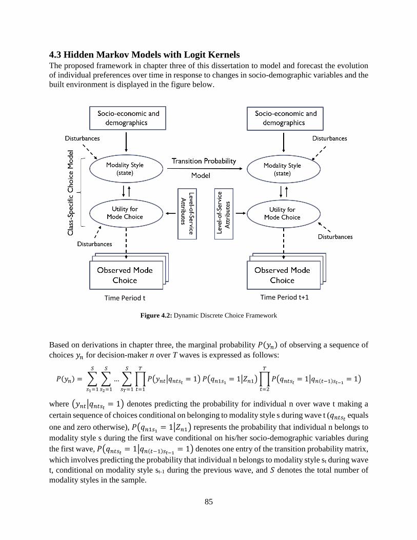
85

4.3 Hidden Markov Models with Logit Kernels The proposed framework in chapter three of this dissertation to model and forecast the evolution

of individual preferences over time in response to changes in socio-demographic variables and the

built environment is displayed in the figure below.

Figure 4.2: Dynamic Discrete Choice Framework

Based on derivations in chapter three, the marginal probability 𝑃(𝑦𝑛) of observing a sequence of

choices 𝑦𝑛 for decision-maker n over T waves is expressed as follows:

𝑃(𝑦𝑛) = ∑ ∑ … ∑ ∏ 𝑃(𝑦𝑛𝑡|𝑞𝑛𝑡𝑠𝑡= 1) 𝑃(𝑞𝑛1𝑠1

= 1|𝑍𝑛1) ∏ 𝑃(𝑞𝑛𝑡𝑠𝑡= 1|𝑞𝑛(𝑡−1)𝑠𝑡−1

= 1)

𝑇

𝑡=2

𝑇

𝑡=1

𝑆

𝑠𝑇=1

𝑆

𝑠2=1

𝑆

𝑠1=1

where (𝑦𝑛𝑡|𝑞𝑛𝑡𝑠𝑡= 1) denotes predicting the probability for individual n over wave t making a

certain sequence of choices conditional on belonging to modality style s during wave t (𝑞𝑛𝑡𝑠𝑡 equals

one and zero otherwise), 𝑃(𝑞𝑛1𝑠1= 1|𝑍𝑛1) represents the probability that individual n belongs to

modality style s during the first wave conditional on his/her socio-demographic variables during

the first wave, 𝑃(𝑞𝑛𝑡𝑠𝑡= 1|𝑞𝑛(𝑡−1)𝑠𝑡−1

= 1) denotes one entry of the transition probability matrix,

which involves predicting the probability that individual n belongs to modality style st during wave

t, conditional on modality style st-1 during the previous wave, and 𝑆 denotes the total number of

modality styles in the sample.

Time Period t Time Period t+1

86

4.3.1 The EM Formulation

Again, as we have seen earlier, the first step of the EM algorithm entails writing the complete log-

likelihood. We will express the complete log-likelihood equation in terms of the corresponding

logit kernels for the class-specific choice model, initialization model, and transition model. Note

that we will restrict the formulation of the transition probability model to entail socio-demographic

variables. The EM algorithm won’t be a suitable approach when the transition model is

parametrized to reflect changes in the built environment through the consumer surplus. Assuming

that the individual modality styles over the waves are no longer latent but are in fact observable

variables, the complete likelihood 𝐿𝐶 can be written as:

𝐿𝐶 = [∏ ∏ ∏ ∏ ∏ [𝑃 (𝑦𝑛𝑡𝑘𝑗

|𝑞𝑛𝑡𝑠

= 1)]𝑦𝑛𝑡𝑘𝑗∗𝑞𝑛𝑡𝑠


𝐾𝑛𝑡

𝑘=1

𝑆

𝑠=1

𝑇

𝑡=1

𝑁

𝑛=1

] [∏ ∏[𝑃(𝑞𝑛1𝑠

= 1|𝑍𝑛1)]𝑞𝑛1𝑠

𝑆

𝑠=1

𝑁

n=1

].

[∏ ∏ ∏ ∏[𝑃(𝑞𝑛𝑡𝑠 = 1|𝑞𝑛(𝑡−1)𝑟 = 1)]𝑞𝑛𝑡𝑠∗𝑞𝑛(𝑡−1)𝑟

𝑆

𝑟=1

𝑆

𝑠=1

𝑇

𝑡=2

𝑁

𝑛=1

]

where yntkj equals one if decision-maker n over wave t and choice situation k chose alternative j

and zero otherwise, Cntk|s denotes the choice set available for individual n at wave t and choice

situation k conditional on modality style s, Knt is the distinct number of choice situations observed

for individual n over wave t, and N represents the total number of individuals in the sample.

Replacing the probability distributions with their corresponding logit kernels:

𝐿𝐶 = [∏ ∏ ∏ ∏ ∏ [𝑒𝑥𝑛𝑡𝑘𝑗

′ 𝛽𝑠

∑ 𝑒𝑥



]

𝑦𝑛𝑡𝑘𝑗∗𝑞𝑛𝑡𝑠


𝐾𝑛𝑡

𝑘=1

𝑆

𝑠=1

𝑇

𝑡=1

𝑁

𝑛=1

] [∏ ∏ [𝑒𝑧𝑛1

′ 𝜏𝑠

∑ 𝑒𝑧𝑛1′ 𝜏𝑠′𝑆

𝑠′=1

]

𝑞𝑛1𝑠𝑆

𝑠=1

𝑁

n=1

].

[∏ ∏ ∏ ∏ [𝑒𝑧𝑛𝑡

′ 𝛾𝑠𝑟

∑ 𝑒𝑧𝑛𝑡′ 𝛾𝑠′𝑟

𝑆𝑠′=1

]

𝑞𝑛𝑡𝑠∗𝑞𝑛(𝑡−1)𝑟𝑆

𝑟=1

𝑆

𝑠=1

𝑇

𝑡=2

𝑁

𝑛=1

]

where xntkj′ is a row vector of attributes of alternative j during choice situation k over wave t for

individual n, βs is a column vector of parameters specific to modality style s, zn1′ is a row vector

of socio-economic and demographic variables for individual n during the first wave and τs is the

associated column vector of parameter estimates for modality style s, znt′ is a row vector of

observable socio-economic and demographic characteristics of individual n over wave t and γsr is

87

a column vector of parameters specific to modality style s at wave t given that the individual

belonged to modality style r during wave (t-1).

The above likelihood function could be expressed as follows:

𝐿𝐶 = [∏ ∏ ∏ ∏ ∏ [𝑒𝑥𝑛𝑡𝑘𝑗

′ 𝛽𝑠

∑ 𝑒𝑥



]

𝑦𝑛𝑡𝑘𝑗∗𝑞𝑛𝑡𝑠


𝐾𝑛𝑡

𝑘=1

𝑆

𝑠=1

𝑇

𝑡=1

𝑁

𝑛=1

] [∏ ∏ [𝑒𝑧𝑛1𝑠

′ 𝜏

∑ 𝑒𝑧𝑛1𝑠′ 𝜏𝑆

𝑠′=1

]

𝑞𝑛1𝑠𝑆

𝑠=1

𝑁

n=1

].

[∏ ∏ ∏ ∏ [𝑒𝑧𝑛𝑡𝑠

′ 𝛾𝑟

∑ 𝑒𝑧𝑛𝑡𝑠′′ 𝛾𝑟𝑆

𝑠′=1

]

𝑞𝑛𝑡𝑠∗𝑞𝑛(𝑡−1)𝑟𝑆

𝑟=1

𝑆

𝑠=1

𝑇

𝑡=2

𝑁

𝑛=1

]

where 𝑧𝑛𝑡𝑠′ is a row vector of socio-economic and demographic variables at wave t that are

interacted with modality style specific binary variables.

The unknown parameter vectors in the above equations are {𝛽, 𝜏, 𝛾}. Taking the logarithm, it can

be seen that the complete log-likelihood function 𝐿𝐶 breaks apart quite conveniently into three

separate components:

𝐿𝐶 = ∑ ∑ ∑ ∑ ∑ 𝑦𝑛𝑡𝑘𝑗𝑞𝑛𝑡𝑠𝑙𝑜𝑔


𝐾𝑛𝑡

𝑘=1

𝑆

𝑠=1

𝑇

𝑡=1

𝑁

𝑛=1

[𝑒𝑥𝑛𝑡𝑘𝑗

′ 𝛽𝑠

∑ 𝑒𝑥



] + ∑ ∑ 𝑞𝑛1𝑠𝑙𝑜𝑔 [𝑒𝑧𝑛1𝑠

′ 𝜏

∑ 𝑒𝑧𝑛1𝑠′ 𝜏𝑆

𝑠′=1

]

𝑆

𝑠=1

𝑁

𝑛=1

+ ∑ ∑ ∑ ∑ 𝑞𝑛𝑡𝑠𝑞𝑛(𝑡−1)𝑟

𝑆

𝑟=1

𝑆

𝑠=1

𝑇

𝑡=2

𝑁

𝑛=1

𝑙𝑜𝑔 [𝑒𝑧𝑛𝑡𝑠

′ 𝛾𝑟


𝑠′=1

]

From the above equation, it is evident that 𝑞𝑛𝑡𝑠 and 𝑞𝑛𝑡𝑠𝑞𝑛(𝑡−1)𝑟 are the sufficient statistics

required for estimating all of the unknown parameters. Let us denote Φ as the vector of unknown

parameters to be estimated = {𝛽, 𝜏, 𝛾}.

4.3.2 The E-step

The following section focuses on the derivations pertinent to the E-step, which requires evaluating

the expectation of every sufficient statistic. Let 𝜋𝑛𝑡𝑠 and 𝜔𝑛𝑡𝑠𝑟 denote the expectations

𝐸[𝑞𝑛𝑡𝑠|𝒚; 𝚽] and 𝐸[𝑞𝑛𝑡𝑠𝑞𝑛(𝑡−1)𝑟 |𝒚; 𝚽] respectively. The updates for 𝜋𝑛𝑡𝑠 and 𝜔𝑛𝑡𝑠𝑟 as given by

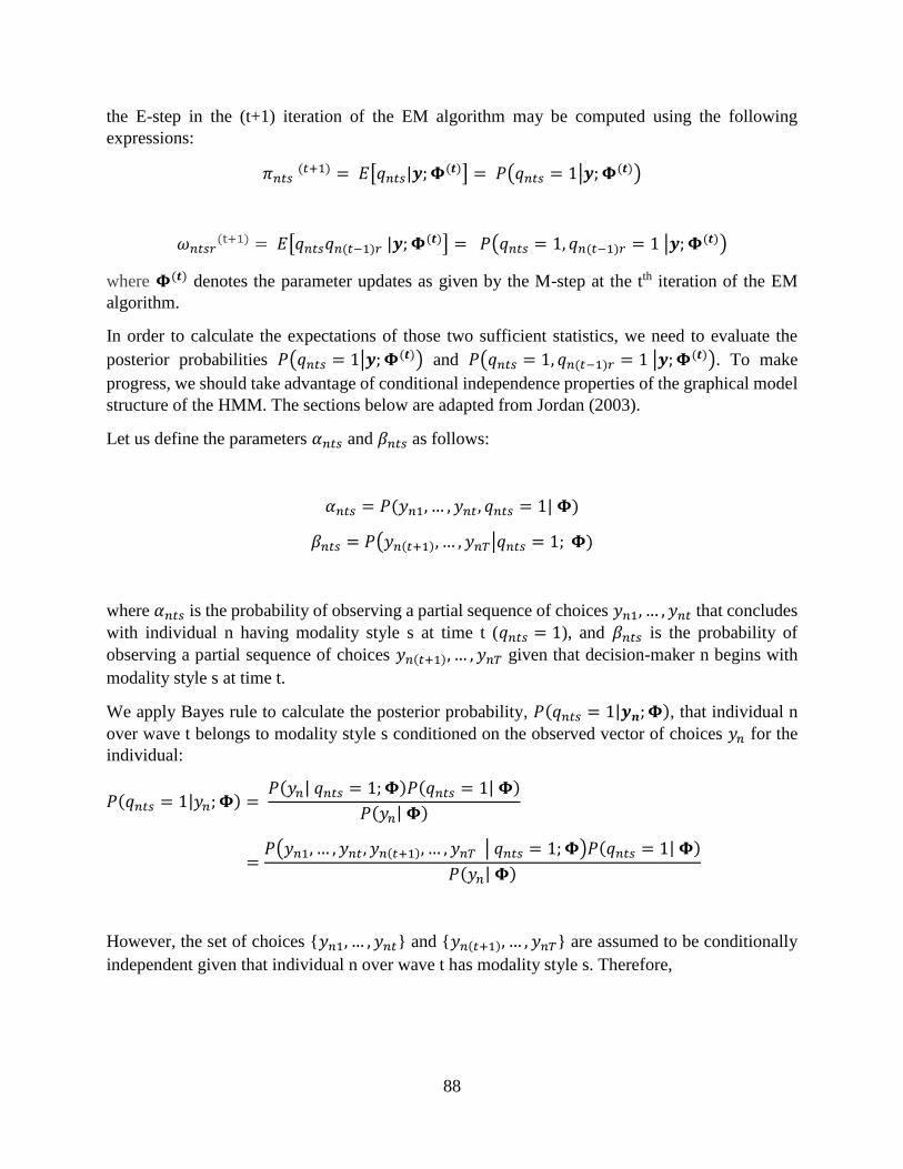
88

the E-step in the (t+1) iteration of the EM algorithm may be computed using the following

expressions:

𝜋𝑛𝑡𝑠 (𝑡+1) = 𝐸[𝑞𝑛𝑡𝑠|𝒚; 𝚽(𝒕)] = 𝑃(𝑞𝑛𝑡𝑠 = 1|𝒚; 𝚽(𝒕))

𝜔𝑛𝑡𝑠𝑟(t+1) = 𝐸[𝑞𝑛𝑡𝑠𝑞𝑛(𝑡−1)𝑟 |𝒚; 𝚽(𝒕)] = 𝑃(𝑞𝑛𝑡𝑠 = 1, 𝑞𝑛(𝑡−1)𝑟 = 1 |𝒚; 𝚽(𝒕))

where 𝚽(𝒕) denotes the parameter updates as given by the M-step at the tth iteration of the EM

algorithm.

In order to calculate the expectations of those two sufficient statistics, we need to evaluate the

posterior probabilities 𝑃(𝑞𝑛𝑡𝑠 = 1|𝒚; 𝚽(𝒕)) and 𝑃(𝑞𝑛𝑡𝑠 = 1, 𝑞𝑛(𝑡−1)𝑟 = 1 |𝒚; 𝚽(𝒕)). To make

progress, we should take advantage of conditional independence properties of the graphical model

structure of the HMM. The sections below are adapted from Jordan (2003).

Let us define the parameters 𝛼𝑛𝑡𝑠 and 𝛽𝑛𝑡𝑠 as follows:

𝛼𝑛𝑡𝑠 = 𝑃(𝑦𝑛1, … , 𝑦𝑛𝑡, 𝑞𝑛𝑡𝑠 = 1| 𝚽)

𝛽𝑛𝑡𝑠 = 𝑃(𝑦𝑛(𝑡+1), … , 𝑦𝑛𝑇|𝑞𝑛𝑡𝑠 = 1; 𝚽)

where 𝛼𝑛𝑡𝑠 is the probability of observing a partial sequence of choices 𝑦𝑛1, … , 𝑦𝑛𝑡 that concludes

with individual n having modality style s at time t (𝑞𝑛𝑡𝑠 = 1), and 𝛽𝑛𝑡𝑠 is the probability of

observing a partial sequence of choices 𝑦𝑛(𝑡+1), … , 𝑦𝑛𝑇 given that decision-maker n begins with

modality style s at time t.

We apply Bayes rule to calculate the posterior probability, 𝑃(𝑞𝑛𝑡𝑠 = 1|𝒚𝒏; 𝚽), that individual n

over wave t belongs to modality style s conditioned on the observed vector of choices 𝑦𝑛 for the

individual:

𝑃(𝑞𝑛𝑡𝑠 = 1|𝑦𝑛; 𝚽) = 𝑃(𝑦𝑛| 𝑞𝑛𝑡𝑠 = 1; 𝚽)𝑃(𝑞𝑛𝑡𝑠 = 1| 𝚽)

𝑃(𝑦𝑛| 𝚽)

=𝑃(𝑦𝑛1, … , 𝑦𝑛𝑡, 𝑦𝑛(𝑡+1), … , 𝑦𝑛𝑇 | 𝑞𝑛𝑡𝑠 = 1; 𝚽)𝑃(𝑞𝑛𝑡𝑠 = 1| 𝚽)


However, the set of choices {𝑦𝑛1, … , 𝑦𝑛𝑡} and {𝑦𝑛(𝑡+1), … , 𝑦𝑛𝑇} are assumed to be conditionally

independent given that individual n over wave t has modality style s. Therefore,

89

𝑃(𝑞𝑛𝑡𝑠 = 1|𝑦𝑛; 𝚽) =𝑃(𝑦𝑛1, … , 𝑦𝑛𝑡|𝑞𝑛𝑡𝑠 = 1; 𝚽)𝑃(𝑦𝑛(𝑡+1), … , 𝑦𝑛𝑇|𝑞𝑛𝑡𝑠 = 1; 𝚽)𝑃(𝑞𝑛𝑡𝑠 = 1|𝚽)


=𝑃(𝑦𝑛1, … , 𝑦𝑛𝑡, 𝑞𝑛𝑡𝑠 = 1| 𝚽)𝑃(𝑦𝑛(𝑡+1), … , 𝑦𝑛𝑇|𝑞𝑛𝑡𝑠 = 1; 𝚽)


= 𝛼𝑛𝑡𝑠𝛽𝑛𝑡𝑠

𝑃(𝑦𝑛| 𝚽)= 𝜋𝑛𝑡𝑠

For any t ∈ {1, …, T}, the following identity will hold true:

𝛼𝑛𝑡𝑠𝛽𝑛𝑡𝑠 = 𝑃(𝑞𝑛𝑡𝑠 = 1|𝑦𝑛; 𝚽)𝑃(𝑦𝑛| 𝚽)

Now, the sum of 𝑃(𝑞𝑛𝑡𝑠 = 1|𝑦𝑛; 𝚽) over the possible values of 𝑞𝑛𝑡𝑠 must equal one. Using this

property we obtain:

∑ 𝛼𝑛𝑡𝑠𝛽𝑛𝑡𝑠 = ∑ 𝑃(𝑞𝑛𝑡𝑠 = 1|𝑦𝑛; 𝚽)𝑃(𝑦𝑛| 𝚽)

𝑆

𝑠=1

= 𝑃(𝑦𝑛| 𝚽)

𝑆

𝑠=1

This implies that we can estimate the likelihood 𝑃(𝑦𝑛| 𝚽) by calculating 𝛼𝑛𝑡𝑠 and 𝛽𝑛𝑡𝑠 for any

wave t and summing their product. This presents a way to calculate the likelihood function for

hidden Markov models. It is evident that our problem of calculating the expectation of the

sufficient statistic, 𝑞𝑛𝑡𝑠, involves calculating the alphas and betas.

From here onwards, for the sake of notational convenience we will not explicitly include 𝚽 in any

of the expressions, but all the probabilities are conditioned on knowing the vector of parameters

𝚽. Also, the indicator value for modality style s of a certain individual n at wave t period will be

represented as 𝑞𝑛𝑡𝑠 instead of (𝑞𝑛𝑡𝑠 = 1) for notational convenience. Now, the variable 𝛼𝑛𝑡𝑠 will

be calculated as follows:

𝛼𝑛𝑡𝑠 = 𝑃(𝑦𝑛1, … , 𝑦𝑛𝑡, 𝑞𝑛𝑡𝑠)

= 𝑃(𝑦𝑛1, … , 𝑦𝑛𝑡|𝑞𝑛𝑡𝑠)𝑃(𝑞𝑛𝑡𝑠)

= 𝑃(𝑦𝑛1, … , 𝑦𝑛(𝑡−1)|𝑞𝑛𝑡𝑠) 𝑃(𝑦𝑛𝑡|𝑞𝑛𝑡𝑠)𝑃(𝑞𝑛𝑡𝑠)

= 𝑃(𝑦𝑛𝑡|𝑞𝑛𝑡𝑠)𝑃(𝑦𝑛1, … , 𝑦𝑛(𝑡−1), 𝑞𝑛𝑡𝑠)

= 𝑃(𝑦𝑛𝑡|𝑞𝑛𝑡𝑠) ∑ 𝑃(𝑦𝑛1, … , 𝑦𝑛(𝑡−1), 𝑞𝑛(𝑡−1)𝑠′ , 𝑞𝑛𝑡𝑠)

𝑆

𝑠′=1

= 𝑃(𝑦𝑛𝑡|𝑞𝑛𝑡𝑠) ∑ 𝑃(𝑦𝑛1, … , 𝑦𝑛(𝑡−1), 𝑞𝑛𝑡𝑠|𝑞𝑛(𝑡−1)𝑠′ )

𝑆

𝑠′=1

𝑃(𝑞𝑛(𝑡−1)𝑠′)

90

= 𝑃(𝑦𝑛𝑡|𝑞𝑛𝑡𝑠) ∑ 𝑃(𝑦𝑛1, … , 𝑦𝑛(𝑡−1)|𝑞𝑛(𝑡−1)𝑠′) 𝑃(𝑞𝑛𝑡𝑠|𝑞𝑛(𝑡−1)𝑠′)

𝑆

𝑠′=1

𝑃(𝑞𝑛(𝑡−1)𝑠′)

= 𝑃(𝑦𝑛𝑡|𝑞𝑛𝑡𝑠) ∑ 𝑃(𝑦𝑛1, … , 𝑦𝑛(𝑡−1), 𝑞𝑛(𝑡−1)𝑠′) 𝑃(𝑞𝑛𝑡𝑠|𝑞𝑛(𝑡−1)𝑠′)

𝑆

𝑠′=1

= 𝑃(𝑦𝑛𝑡|𝑞𝑛𝑡𝑠) ∑ 𝛼𝑛(𝑡−1)𝑠′ 𝑃(𝑞𝑛𝑡𝑠|𝑞𝑛(𝑡−1)𝑠′)

𝑆

𝑠′=1

The algorithm proceeds “forward” in time to compute alphas for all t ∈ {1, …, T}. For the first

time period, i.e. t=1, the algorithm may be initialized as follows:

𝛼𝑛1𝑠 = 𝑃(𝑦𝑛1, 𝑞𝑛1𝑠)

= 𝑃(𝑦𝑛1|𝑞𝑛1𝑠)𝑃(𝑞𝑛1𝑠)

The variable 𝛽𝑛𝑡𝑠 may be calculated recursively via a “backward” recursion according to the

following set of derivations:

𝛽𝑛(𝑡−1)𝑠 = 𝑃(𝑦𝑛𝑡, … , 𝑦𝑛𝑇|𝑞𝑛(𝑡−1)𝑠)

= ∑ 𝑃(𝑦𝑛𝑡, … , 𝑦𝑛𝑇 , 𝑞𝑛𝑡𝑠′|𝑞𝑛(𝑡−1)𝑠)

𝑆

𝑠′=1

= ∑ 𝑃(𝑦𝑛𝑡, … , 𝑦𝑛𝑇|𝑞𝑛(𝑡−1)𝑠, 𝑞𝑛𝑡𝑠′)P(𝑞𝑛𝑡𝑠′ |𝑞𝑛(𝑡−1)𝑠)

𝑆

𝑠′=1

= ∑ 𝑃(𝑦𝑛𝑡| 𝑞𝑛𝑡𝑠′)𝑃(𝑦𝑛(𝑡+1), … , 𝑦𝑛𝑇| 𝑞𝑛𝑡𝑠′)P(𝑞𝑛𝑡𝑠′ |𝑞𝑛(𝑡−1)𝑠)

𝑆

𝑠′=1

= ∑ 𝑃(𝑦𝑛𝑡| 𝑞𝑛𝑡𝑠′)𝛽𝑛𝑡𝑠′P(𝑞𝑛𝑡𝑠′ |𝑞𝑛(𝑡−1)𝑠)

𝑆

𝑠′=1

This time the algorithm starts at the final wave t = T and proceeds backward in time. For t = T, the

algorithm cannot use the definition of 𝛽𝑛𝑇𝑠 since it relies on non-existent 𝑦𝑛(𝑇+1). However, if we

define 𝛽𝑛𝑇𝑠 = 1 for all n ∈ {1, …, N} and s ∈ {1, …, S}, then we can apply the above backward

recursion equation to show that 𝛽𝑛(𝑇−1)𝑠 will be calculated correctly as follows:

𝛽𝑛(𝑇−1)𝑠 = ∑ 𝑃(𝑦𝑛𝑇| 𝑞𝑛𝑇𝑠′)𝛽𝑛𝑇𝑠′P(𝑞𝑛𝑇𝑠′ |𝑞𝑛(𝑇−1)𝑠)

𝑆

𝑠′=1

91

= ∑ 𝑃(𝑦𝑛𝑇| 𝑞𝑛𝑇𝑠′)P(𝑞𝑛𝑇𝑠′ |𝑞𝑛(𝑇−1)𝑠)

𝑆

𝑠′=1

= ∑ 𝑃(𝑦𝑛𝑇| 𝑞𝑛𝑇𝑠′ , 𝑞𝑛(𝑇−1)𝑠)P(𝑞𝑛𝑇𝑠′ |𝑞𝑛(𝑇−1)𝑠)

𝑆

𝑠′=1

= ∑ 𝑃(𝑦𝑛𝑇 , 𝑞𝑛𝑇𝑠′| 𝑞𝑛(𝑇−1)𝑠) = 𝑃(𝑦𝑛𝑇| 𝑞𝑛(𝑇−1)𝑠)

𝑆

𝑠′=1

Therefore, the initialization definition makes sense.

To calculate the expectation of the other sufficient statistic 𝑞𝑛𝑡𝑠𝑞𝑛(𝑡−1)𝑟, we need to calculate the

posterior probability 𝑃(𝑞𝑛𝑡𝑠 = 1, 𝑞𝑛(𝑡−1)𝑟 = 1 | 𝑦𝑛), denoted by 𝜔𝑛𝑡𝑠𝑟, as follows:

𝜔𝑛𝑡𝑠𝑟 = 𝑃(𝑞𝑛𝑡𝑠 = 1, 𝑞𝑛(𝑡−1)𝑟 = 1 | 𝑦𝑛)

= 𝑃( 𝑦𝑛| 𝑞𝑛𝑡𝑠, 𝑞𝑛(𝑡−1)𝑟)𝑃( 𝑞𝑛𝑡𝑠|𝑞𝑛(𝑡−1)𝑟)𝑃(𝑞𝑛(𝑡−1)𝑟)

𝑃(𝑦𝑛)

= 𝑃(𝑦𝑛1,…,𝑦𝑛(𝑡−1)| 𝑞𝑛(𝑡−1)𝑟)𝑃( 𝑦𝑛𝑡| 𝑞𝑛𝑡𝑠)𝑃(𝑦𝑛(𝑡+1),…,𝑦𝑛𝑇| 𝑞𝑛𝑡𝑠)𝑃( 𝑞𝑛𝑡𝑠|𝑞𝑛(𝑡−1)𝑟)𝑃(𝑞𝑛(𝑡−1)𝑟)

𝑃(𝑦𝑛)

= 𝑃(𝑦𝑛1,…,𝑦𝑛(𝑡−1), 𝑞𝑛(𝑡−1)𝑟)𝑃( 𝑦𝑛𝑡| 𝑞𝑛𝑡𝑠)𝑃(𝑦𝑛(𝑡+1),…,𝑦𝑛𝑇| 𝑞𝑛𝑡𝑠)𝑃(𝑞𝑛𝑡𝑠|𝑞𝑛(𝑡−1)𝑟)

𝑃(𝑦𝑛)

= 𝛼𝑛(𝑡−1)𝑟𝑃( 𝑦𝑛𝑡| 𝑞𝑛𝑡𝑠)𝛽𝑛𝑡𝑠 𝑃(𝑞𝑛𝑡𝑠|𝑞𝑛(𝑡−1)𝑟)

𝑃(𝑦𝑛)

4.3.3 The M-Step

Having derived expressions for the updates in the E-step for both sufficient statistics, we can

proceed now to the M-step. Taking the derivative of the complete log-likelihood with respect to

the unknown parameters, we get the following updates for the M-step:

𝛽𝑠(𝑡+1)

= 𝑎𝑟𝑔𝑚𝑎𝑥𝛽𝑠∑ ∑ ∑ ∑ 𝑦𝑛𝑡𝑘𝑗 𝜋𝑛𝑡𝑠 (𝑡+1)


𝐾𝑛𝑡

𝑘=1

𝑇

𝑡=1

𝑙𝑜𝑔

𝑁

𝑛=1


′ 𝛽s

∑ 𝑒𝑥

𝑛𝑡𝑘𝑗′′ 𝛽s


]

92

𝜏(𝑡+1) = 𝑎𝑟𝑔𝑚𝑎𝑥𝜏 ∑ ∑ 𝜋𝑛1𝑠 (𝑡+1) 𝑙𝑜𝑔 [𝑒𝑧𝑛1𝑠

′ 𝜏

∑ 𝑒𝑧𝑛1𝑠′′ 𝜏𝑆

𝑠′=1

]

𝑆

𝑠=1

𝑁

𝑛=1

𝛾𝑟(𝑡+1) = 𝑎𝑟𝑔𝑚𝑎𝑥𝛾𝑟

∑ ∑ ∑ 𝜔𝑛𝑡𝑠𝑟(t+1) 𝑙𝑜𝑔 [

𝑒𝑧𝑛𝑡𝑠′ 𝛾𝑟


𝑠′=1

]

𝑆

𝑠=1

𝑇

𝑡=2

𝑁

𝑛=1

Those three equations are weighted multinomial logit models that can be solved fairly efficiently.

The EM algorithm iterates between the E-step and the M-step, until the convergence criterion is

satisfied.

4.3.4 Gradient for Weighted Multinomial Logit Modal

We will focus on the derivation of the gradient for a weighted multinomial logit model, building

off the derivation from the static mixture model (LCCM). The log-likelihood function for a

weighted multinomial logit model in the case of the class-specific choice model is given by:

𝐿 = ∑ ∑ ∑ ∑ 𝑦𝑛𝑡𝑘𝑗 𝜋𝑛𝑡𝑠


𝐾𝑛𝑡

𝑘=1

𝑇

𝑡=1

𝑙𝑜𝑔

𝑁

𝑛=1


′ 𝛽s

∑ 𝑒𝑥



]

Let us define the weight vector, 𝑤𝑛𝑡𝑘𝑗 = 𝑦𝑛𝑡𝑘𝑗𝜋𝑛𝑡𝑠 and 𝑃𝑛𝑡𝑘𝑗 = 𝑒

𝑥𝑛𝑡𝑘𝑗′ 𝛽s

∑ 𝑒𝑥



.Then,

𝐿 = ∑ ∑ ∑ ∑ 𝑤𝑛𝑡𝑘𝑗


𝐾𝑛𝑡

𝑘=1

𝑇

𝑡=1

𝑙𝑜𝑔

𝑁

𝑛=1


′ 𝛽s

∑ 𝑒𝑥



]

= ∑ ∑ ∑ ∑ 𝑤𝑛𝑡𝑘𝑗𝑥𝑛𝑡𝑘𝑗′ 𝛽s


𝐾𝑛𝑡

𝑘=1

𝑇

𝑡=1

− ∑ ∑ ∑ ∑ 𝑤𝑛𝑡𝑘𝑗


𝐾𝑛𝑡

𝑘=1

𝑇

𝑡=1

log [ ∑ 𝑒𝑥



]

𝑁

𝑛=1

𝑁

𝑛=1


𝑑𝐿

𝑑𝛽s= ∑ ∑ ∑ ∑ 𝑤𝑛𝑡𝑘𝑗𝑥𝑛𝑡𝑘𝑗

′


𝐾𝑛𝑡

𝑘=1

𝑇

𝑡=1

𝑁

𝑛=1

− ∑ ∑ ∑ ∑ 𝑤𝑛𝑡𝑘𝑗


𝐾𝑛𝑡

𝑘=1

𝑇

𝑡=1

∑ 𝑥𝑛𝑡𝑘𝑗′′ 𝑃𝑛𝑡𝑘𝑗′


𝑁

𝑛=1

= ∑ ∑ ∑ ∑ 𝑤𝑛𝑡𝑘𝑗𝑥𝑛𝑡𝑘𝑗′


𝐾𝑛𝑡

𝑘=1

𝑇

𝑡=1

𝑁

𝑛=1

− ∑ ∑ ∑ ∑ 𝑥𝑛𝑡𝑘𝑗′′ 𝑃𝑛𝑡𝑘𝑗′


∑ 𝑤𝑛𝑡𝑘𝑗


𝐾𝑛𝑡

𝑘=1

𝑇

𝑡=1

𝑁

𝑛=1

93

= ∑ ∑ ∑ ∑ [𝑤𝑛𝑡𝑘𝑗 − 𝑃𝑛𝑡𝑘𝑗 ∑ 𝑤𝑛𝑡𝑘𝑗′


]


𝐾𝑛𝑡

𝑘=1

𝑇

𝑡=1

𝑁

𝑛=1

𝑥𝑛𝑡𝑘𝑗′

However, for similar reasons as the class-specific choice model for the latent class choice model,

∑ 𝑤𝑛𝑡𝑘𝑗′𝑗′∈ 𝐶𝑛𝑡𝑘|𝑠 = 1.

Thus,

𝑑𝐿

𝑑𝛽s= ∑ ∑ ∑ ∑ [𝑤𝑛𝑡𝑘𝑗 − 𝑃𝑛𝑡𝑘𝑗]


𝐾𝑛𝑡

𝑘=1

𝑇

𝑡=1

𝑁

𝑛=1

𝑥𝑛𝑡𝑘𝑗′

Similarly based on the derivations of the above weighted multinomial logit model, the gradients

for the remaining parameters are computed as follows:

𝑑𝐿

𝑑𝜏= ∑ ∑[𝜋𝑛1𝑠 − 𝑃𝑛1𝑠] 𝑧𝑛1𝑠

′

𝑆

𝑠=1

𝑁

𝑛=1

where 𝑃𝑛1𝑠 = 𝑒𝑧𝑛1𝑠

′ 𝜏

∑ 𝑒𝑧𝑛1𝑠′′ 𝜏𝑆

𝑠′=1

𝑑𝐿

𝑑𝛾𝑟= ∑ ∑ ∑[𝜔𝑛𝑡𝑠𝑟 − 𝑃𝑛𝑡𝑠𝑟] 𝑧𝑛𝑡𝑠

′ where 𝑃𝑛𝑡𝑠𝑟 = 𝑒𝑧𝑛𝑡𝑠

′ 𝛾𝑟


𝑠′=1

𝑆

𝑠=1

𝑇

𝑡=2

𝑁

𝑛=1

Again, we can clearly see that the gradient for weighted multinomial logit models has a closed

form, which is the case for all sets of parameters in our HMM. This will be very beneficial from

an optimization perspective in reducing computation and estimation time.

4.4 Conclusion Estimating advanced discrete choice models, such as mixture models or hidden Markov models

with logit kernels are prone to numerical difficulty when maximizing the likelihood function using

tradition gradient descent techniques. The EM algorithm is an alternative procedure for

maximizing the likelihood for models that entail discrete latent variables. The EM algorithm is a

more stable alternative approach, which involves maximizing functions that are much easier to be

maximized as opposed to the model’s full likelihood function. In this chapter, we provide rigorous

derivations of the various steps of the EM algorithm for both mixture models and hidden Markov

models with logit kernels, in addition to the closed form gradients. Our objective is to enable travel

demand and behavioral modelers to estimate such advanced models while saving on computation

and estimation time.

94

Chapter 5

Conclusion

5.1 Summary We started our discussion in this dissertation by identifying the need for developing quantitative

methods to model and predict trends of travel behavior in response to major technological and

infrastructural changes. Understanding travel behavior in this era of transformative mobility is key

to assessing how policies and investment strategies can transform cities to provide a higher level

of connectivity, improve the economic and environmental health for people, attain significant

reductions in congestion levels, and encourage multimodality. In addition to that, literature

suggests that over time, travel choices, attitudes, and social norms will result in changes in

lifestyles and travel behavior. Hence, dynamic modeling of changes in lifestyles and behavior in

response to infrastructural and technological investments is central to modeling and influencing

trends of travel behavior, and improving long-range forecasting accuracy. Current travel demand

models do not reflect such dynamics, which becomes questionable in times such as the present.

In order to account for all of the aforementioned limitations and needs, we develop a disaggregate,

dynamic discrete choice framework to model and predict long-range trends of travel behavior to

account for upcoming technological and infrastructural changes (see figure 5.1 below). The

building blocks of this proposed framework were developed and tested to empirically highlight

the value of the framework to transportation policy and practice.

The proposed disaggregate, dynamic discrete choice framework in this dissertation addresses two

key limitations of existing travel demand models, specifically:

1- Trends of evolution of preferences, lifestyles and transport modality styles in response to

changes in socio-demographic variables and the built environment.

2- Trends of technology and service adoption, in order to gain insight about the projected

market shares of upcoming modes of transport.

This dissertation also provides the derivation and formulation of the Expectation Maximization

(EM) algorithm in the context of discrete mixture models and hidden Markov models with logit

kernels to save on computation and estimation time. Such a statistical technique becomes

extremely useful to travel demand and behavioral modelers when estimating advanced models.

95

Figure 5.1: Proposed Disaggregate, Dynamic Discrete Choice Framework

The building blocks of the proposed dynamic, disaggregate discrete choice framework were

estimated on two different datasets. The first component focuses on estimating a disaggregate

technology adoption model with a discrete choice kernel. This component integrates a network

effect and latent class choice model to understand and forecast the adoption and diffusion of

upcoming modes of transportation (see figure 5.2 below). The second component focuses on

estimating hidden Markov models with logit kernels to model and forecast the evolution of

preferences, lifestyles and transport modality styles over time in response to changes in socio-

demographic variables and the built environment. This component quantifies the evolution of

lifestyles and modality styles over time in response to policies and investment strategies (see figure

5.3). The developed methodological framework in this dissertation will in turn project the market

share of modes of transportation in a more representative manner in the long run.

Throughout the previous chapters of the dissertation, we provided model estimation results using

two datasets to test and demonstrate the use, practicality and methodological robustness of the

proposed framework.

96


Figure 5.3: Dynamic Discrete Choice Framework

Time Period t Time Period t+1

97

The generalized technology adoption model, which was developed and tested in chapter 2, is

rooted in the technology diffusion literature that identifies two distinct types of adopters:

innovators and imitators. Our framework builds on the formulation of dynamic latent class choice

models, which were integrated with a network effect model. We were interested in developing a

network effect model to understand how the size of the network, governed by the new mode of

transportation, influences the adoption behavior of the different market segments. A confirmatory

approach was adopted to estimating our dynamic latent class choice model based on findings from

the technology diffusion literature that focus on defining two distinct types of adopters:

innovators/early adopters and imitators. The technology adoption model predicts the probability

that a certain individual will adopt the service at a certain time period, and is explained by social

influences, network effect, socio-demographics and level-of-service attributes. There are two key

contributions in our methodological framework: (1) capturing heterogeneity in the adoption utility

among different market segments; and (2) capturing the impact of the spatial/network effect of the

new technology on the utility of adoption. The proposed adoption model is powerful in terms of

forecasting the number of adopters for different policies and investment strategies into the future.

The dynamic discrete choice model, which was developed and tested in chapter 3, models the

evolution of preferences, lifestyles, and transport modality styles over time. The contribution in

this chapter is to develop, apply, and test an HMM framework to capture, model and forecast the

evolution of individual preferences and behaviors over long-range forecasting horizons. The

methodological framework focuses on developing a structural approach for modeling the evolution

of preferences over time due to changes in socio-demographic variables and the built environment.

The construct of modality styles is used to denote preferences states. It is those modality style

preference states that evolve dynamically over time. Model results depict that preference states,

denoted by modality styles, did indeed shift and evolve over time as a result of changes in the

transportation system. Preferences of individuals have shifted in terms of their choice set

consideration and sensitivities to level-of-service attributes. This dynamic choice model entails a

richer behavioral dimension and will in turn quantify the influence of policies and investment

strategies on the projected market shares of the modes of transport more accurately in the long run.

Both methodological frameworks in this dissertation employ the Expectation Maximization (EM)

algorithm for model estimation. The required formulation, derivation, and application of the EM

algorithm in the context of discrete mixture models and hidden Markov models with logit kernels

to save on computation and estimation time denote the third component of this dissertation, and

were presented in chapter 4.

98

5.2 Research Directions The proposed dynamic, disaggregate discrete choice framework in this dissertation requires further

investigations across multiple dimensions to enhance its empirical flexibility and robustness. That

said, future directions pertinent to the proposed framework entail the following:

1- Rigorous data collection in terms of collecting panel data of travel and activity behavior while

accounting for the uptake of new modes of transportation such as carsharing and ridesharing.

This will enable us to estimate the joint proposed dynamic, disaggregate discrete choice

framework (figure 5.1), which is required to understand and predict long-range trend of travel

behavior. Estimating the joint framework allows us to model how modality styles can impact

adoption styles in order to understand how adoption and diffusion of new technologies and

services will be influenced by habits, and lifestyles built around the use of a certain subset of

travel modes.

2- The discrete choice framework of adoption and diffusion of new transportation services that

was developed in chapter 2 of this dissertation fails to account for the effect of competition

between various modes of transport, new technologies and services. Future extensions of this

framework will allow us to understand how the diffusion of carsharing and ridesharing services

will evolve over time as those new modes compete with each other in terms of capturing

ridership. This will improve the accuracy of projected demand and minimize the bound of its

confidence interval.

3- The validation of the hidden Markov model presented in chapter 3 of this dissertation has

focused merely on statistical and goodness of fit measures: �̅�2, AIC and BIC. We also rely on

examining the behavioral richness that is represented and captured by the model framework.

More work needs to be done with respect to model validation, which is more aligned with the

field of machine learning. It will be better to have a validation sample of the data (hold-out)

whereby we train the model on an estimation dataset and determine model accuracy on the

validation dataset. Such an approach was conducted in the adoption and diffusion framework

in chapter 2 whereby we generated confidence intervals for predicted demand on a validation

dataset and evaluated discrepancies between those confidence intervals and actual demand.

4- Both methodological frameworks of chapters 2 and 4 do not incorporate the effects of social

norms, psychometric and psychological constructs of attitudes and perceptions into the

decision-making process. In our methodological framework, the impacts of social norms,

attitudes and perceptions were confounded with the alternative specific constants of the

respective utility equations. For example, it will be important to quantify the effects and shifts

in attitudes (e.g. towards/away from auto-orientation, environmental consciousness, etc.) on

adoption, travel and activity behavior. When social norms, attitudes and perceptions comprise

99

a major determinant of adoption, travel and activity behavior, then it is critical that we quantify

their effects explicitly. If we don’t, omitted variable bias can become worrisome and the

estimated parameters could become inconsistent.

5- This dissertation is rooted in addressing limitations of existing travel demand models in

modeling and forecasting the evolution of trends of travel behavior in response to

transformative technologies and services. The scope of the proposed methodological

framework of chapter 1 could be extended to more medium and long-term dimensions of travel

and activity behavior, for example car ownership and residential choice location. Residential

choice location decisions and car ownership levels are to be conditioned on modality styles

and adoption styles. While such a framework will cater for the dynamic evolution of

preferences over time in addition to the adoption and diffusion of new transportation services,

it will also capture the influence of adoption styles and modality styles on those long-term

decisions. This will allow us to evaluate the impact of policies and investment strategies on

several dimensions of the mobility decision bundle. Such a framework will enable us to

understand how to: (1) influence trends of travel behavior to be more sustainable and

multimodal and more aligned with the envisioned sharing economy future; (2) guide adoption

styles to increase the adoption and diffusion of carsharing and ridesharing services; (3)

significantly reduce car ownership levels to mitigate congestion and greenhouse gas emissions

by effectively nudging and influencing lifestyles; and (4) transform cities in terms of residential

choice location by encouraging urban sprawl away from congested cities through influencing

preferences and modality styles in the right direction followed by nudging adoption styles to

encourage the adoption of ridesharing, carsharing, and autonomous vehicles.

100

5.3 Conclusion Travel demand models constitute a critical component in transportation planning and policy.

Travel demand models used in practice have shifted over the years to constitute disaggregate

models of decision-making as opposed to aggregate models. Current disaggregate activity-based

travel demand models entail a sequence of models that tackle different dimensions of the decision-

making process at the individual and household levels such as mode choice, residential location,

etc. Such models are used to forecast market shares of biking and walking, transit ridership and

traffic volumes that are the result of large scale transportation investments and policy decisions.

However, travel demand models currently used in practice lack a methodological framework that

is required to model and forecast long-range trends of travel behavior in response to upcoming

technologies and services, for example ridesharing, carsharing and autonomous vehicles.

Moreover, the range of travel choices will be wider over time, which in turn influences lifestyles

and travel behavior. Hence, dynamic modeling of changes in lifestyles and behavior in response

to infrastructural and technological investments is central to modeling and influencing trends of

travel behavior, improving long-range forecasting accuracy, and guiding transformative mobility

towards a more sustainable, equitable and efficient system.

The proposed dynamic, disaggregate discrete choice framework of this dissertation entails

advanced models. This however comes at a cost in terms of prolonged computation and estimation

times. This dissertation tries to account for this issue by providing the derivation and formulation

of the EM algorithm for mixture models and hidden Markov models with logit kernels, which are

the building blocks of the generalized dynamic framework. As such, this shall offer a greater

potential to understand and predict behavior, improve forecasting accuracy, influence lifestyles

and trends of travel behavior to be more sustainable and multimodal, and test behavioral

hypotheses. The framework presented in this dissertation is flexible, theoretically grounded,

empirically tested and verified, and behaviorally rich.

This dissertation brings together techniques and tools from machine learning, econometrics

(particularly discrete choice analysis), and the technology diffusion literature. The disaggregate

technology adoption model of chapter 2 is rooted in the diffusion literature and tries to understand

the dynamic adoption behavior of the different market segments over time. In addition to that, we

blend machine learning methods, and in particular hidden Markov models that are widely used in

speech recognition, with discrete choice kernels to model and forecast the evolution of individual

preferences and behaviors over long-range forecasting horizons. We believe that attaining accurate

long-range forecasts lies in bringing those three worlds together. Behavioral modeling of decision-

makers, which is rooted in the discrete choice modeling domain, is a key ingredient in our analysis.

We strongly believe that integrating such techniques with machine learning methods, the

technology diffusion literature, and statistical learning techniques, in particular the EM algorithm

will: (1) enable us to model the complicated decision making process more accurately while saving

on computation time; (2) allow for interpretation of model results as desired by policy makers; and

(3) add richness to the behavioral process represented by the models.

101

Trends of travel behavior are evolving as new technologies and services are introduced. Over the

coming decades, this evolution could play out in utopian or dystopian scenarios or anywhere in

between. The proposed methodological frameworks in this dissertation entail the building blocks

to advances in travel demand modeling required to influence trends of travel behavior and guide

transformative mobility towards a sustainable, efficient and equitable system. Throughout the

dissertation, empirical results are presented to highlight findings and to empirically demonstrate

and test the proposed frameworks in the case of transformative mobility.

102

Bibliography Aarts, H., Verplanken, B., and Knippenberg, A. Habit and Information Use in Travel Mode

Choices. Acta Psychologica, Vol. 96, 1997, pp. 1-14.

Abou-Zeid, M., Rossi, T., and Gardner, B. Modeling Time-of-Day Choice in Context of Tour- and

Activity Based Models. Transportation Research Record: Journal of the Transportation Research

Board, No. 1981, 2006, pp. 42- 49

Bahamonde-Birke, F. J., Kunert, U., Link, H., and de Dios Ortúzar, J. About Attitudes and

Perceptions: Finding the Proper Way to Consider Latent Variables in Discrete Choice Models.

Transportation, 2015, pp.1-19.

Banister, D. The Influence of Habit Formation on Modal Choice - a Heuristic Model.

Transportation, Vol. 7, 1978, pp. 5-33.

Bass, F.M. A New Product Growth for Model Consumer Durables. Management Science, Vol. 15,

No. 5, 1969, pp.215–227.

Baum, L. E., and Petrie, T.P. Statistical Inference for Probabilistic Functions of Finite State

Markov Chains. Annals of Mathematical Statistics, Vol. 37, 1966, pp. 1554-1563.

Baum, L. E., Petrie, T., Soules, G., and Weiss, N. A Maximization Technique Occurring in the

Statistical Analysis of Probabilistic Functions of Markov Chains. The Annals of Mathematical

Statistics, Vol. 41, No. 1, 1970, pp. 164-171.

Becker, G. S. Accounting for Tastes. Harvard University Press, 1996.

Becker, G. S. Habits, Addictions, and Traditions. Kyklos, Vol. 45, No. 3, 1992, pp. 327-345.

Ben-Akiva, M., and Lerman, S. Discrete Choice Analysis. The MIT Press, 1985.

Bhat, C. R. 1997. An Endogenous Segmentation Mode Choice Model with an Application to

Intercity Travel. Transportation Science, Vol. 31, 1997, pp. 34-48.

Bhat, C. R., and Koppelman, F. S. Activity-based Modeling of Travel Demand. In Handbook of

Transportation Science, 1999, pp. 35-61.

Bronnenberg, B. J., Dubé, J. H., and Gentzkow, M. The Evolution of Brand Preferences: Evidence

from Consumer Migration. American Economic Review, Vol. 102, No. 6, 2012, pp. 2472-2508.

Brown, M. Catching the PHEVer: Simulating Electric Vehicle Diffusion with an Agent-Based

Mixed Logit Model of Vehicle Choice, Journal of Artificial Societies and Social Simulation, 2013,

Vol. 16, Issue 5.

Brownstone, D., Bunch, D.S., and Train, K. Joint Mixed Logit Models of Stated and Revealed

Preferences for Alternative-Fuel Vehicles. Transportation Research Part B: Methodological, Vol.

34, No. 5, 2000, pp. 315-338.

Buss, D. M., Shackelford, T. K., Kirkpatrick, L. A., and Larsen, R. J. A Half Century of Mate

Preferences: The Cultural Evolution of Values. Journal of Marriage and Family, Vol. 63, No. 2,

2001, pp. 491-503.

http://www.sciencedirect.com/science/article/pii/S0001691897000085


103

Cambridge Systematics. San Francisco Travel Demand Forecasting Model Development:

Executive Summary. Prepared for San Francisco County Transportation Authority, 2002.

Cantillo, V., Ortúzar, J. de D., and Williams, H. C. W. L. Modeling Discrete Choices in the

Presence of Inertia and Serial Correlation. Transportation Science, Vol. 41, No. 2, 2007, pp. 195-

205.

Carrel, A., Sengupta, R., and Walker, J. L. Understanding Future Mode Choice Intentions of

Transit Riders as a Function of Past Experiences with Travel Quality. In 14th International

Conference on Travel Behaviour Research, Windsor, United Kingdom, 2015.

Cavusoglu, H., Hu, N., Li, Y., and Ma, D. Information Technology Diffusion with Influentials,

Imitators, and Opponents. Journal of Management Information Systems, Vol. 27, 2010, pp. 305-

334.

Choudhury, C. F., Ben-Akiva, M., and Abou-Zeid, M. Dynamic Latent Plan Models. Journal of

Choice Modelling, Vol. 3, No. 2, 2010, pp. 50-70.

Cirillo, C. and Xu, R. Dynamic Discrete Choice Models for Transportation. Transport Reviews,

Vol. 31, No. 4, 2011, pp. 473-494.

Collet, R. Household Car Use in France: a Demographic and Economic Analysis. Economics

Bulletin, Vol. 32, No. 1, 2012, pp.475-485.

Dalvi, M., and Martin, K. The Measurement of Accessibility: Some Preliminary Results.

Transportation 5, 1976, pp. 17-42.

David, P.A. A Contribution to The Theory of Diffusion. Stanford Center for Research in Economic

Growth, Memorandum, 71, 1969.

Dargay, J., and Gately, D. Income’s Effect on Car and Vehicle Ownership, Worldwide: 1960-

2015. Transportation Research Part A: Policy and Practice, Vol. 33, 1999, pp.101–138.

Delre, S.A., Jager, W., Bijmolt, T.H.A., and Janssen, M.A. Targeting and Timing Promotional

Activities: An Agent-based Model for the Takeoff of New Products. Journal of Business Research,

Vol. 60, 2007, pp. 826–835.

Dempster, A., Laird, N., and Rubin, D. Maximum Likelihood from Incomplete Data via the EM

Algorithm. Journal of the Royal Statistical Society Series B, Vol. 39, No. 1, 1977, pp. 1-38.

Desiraju, R., Harikesh N., and Pradeep C. Diffusion of New Pharmaceutical Drugs in Developing

and Developed Nations. International Journal of Research in Marketing, Vol. 21, 2004, pp. 341-

357.

Elster, J. Sour Grapes. Cambridge University Press, 2016.

Eppstein, M., Grover, D., Marshall, J., and Rizzo, D. An Agent-based Model to Study Market

Penetration of Plug-in Hybrid Electric Vehicles, Energy Policy, Vol. 39, 2011, pp. 3789-3802.

Faulkner, G. E., Buliung, R. N., Flora, P. K., and Fusco, C. Active School Transport, Physical

Activity Levels and Body Weight of Children and Youth: a Systematic Review. Preventive

Medicine, Vol. 48, No. 1, 2009, pp. 3-8.


104

Fernández, J. E., de Cea Ch, J. and Malbran, R. H. Demand Responsive Urban Public Transport

System Design: Methodology and Application. Transportation Research Part A, Vol. 42, No. 7,

2008, pp. 951-972.

Garceau, T., Atkinson-Palombo, C. and Garrick, N. Peak Travel and the Decoupling of Vehicle

Travel from the Economy: A Synthesis of the Literature. Transportation Research Record: Journal

of the Transportation Research Board, No. 2412, 2014, pp. 41-48.

Gärling, T., and Axhausen, K. Introduction: Habitual Travel Choice. Transportation, Vol. 30,

2003, pp. 1–11.

George, R. Measuring Change in Students' Attitudes toward Science over Time: An Application

of Latent Variable Growth Modeling. Journal of Science Education and Technology, Vol. 9, No.

3, 2000, pp. 213-225.

Glerum, A., Frejinger, E., Karlstrom, A., Hugosson, M., and Bierlaire, M. Modeling Car

Ownership and Usage: A Dynamic Discrete-Continuous Choice Modeling Approach. Third

International Choice Modelling Conference, 2013.

Glerum, A., Stankovikj, L., Thémans, M. and Bierlaire, M. Forecasting the Demand for Electric

Vehicles: Accounting for Attitudes and Perceptions. Transportation Science, Vol. 48, No. 4, 2013,

pp. 483-499.

Gnann, T., Plötz, P., Kühn, A., and Wietschel, M. Modelling Market Diffusion of Electric Vehicles

with Real World Driving Data – German Market and Policy Options. Transportation Research Part

A, 2015, pp. 95-112.

Goodwin, P. and Van Dender, K. ‘Peak car’—Themes and Issues. Transport Reviews, Vol. 33,

No. 3, 2013, pp. 243-254.

Gopinath, D. A. Modeling Heterogeneity in Discrete Choice Processes: Application to Travel

Demand. PhD Dissertation, Massachusetts Institute of Technology, 1995.

Gorman, W.M. Tastes, Habits and Choices. International Economic Review, Vol. 8, No. 2, 1967,

pp. 218-222.

Goulias, K. G. Longitudinal Analysis of Activity and Travel Pattern Dynamics Using Generalized

Mixed Markov Latent Class Models. Transportation Research Part B, Vol. 33, No. 8, 1999, pp.

535-558.

Griliches, Z. Hybrid Corn: An Exploration in The Economics of Technological Change.

Econometrica, Journal of The Econometric Society, 1957, pp. 501–522.

Guerra, E. Planning for Cars that Drive Themselves: Metropolitan Planning Organizations,

Regional Transportation Plans, and Autonomous Vehicles. Journal of Planning Education and

Research, 2015, pp. 1-15.

Gum, A. M., Areán, P. A., Hunkeler, E., Tang, L., Katon, W., Hitchcock, P., Steffens, D. C.,

Dickens, J., and Unützer, J. Depression Treatment Preferences in Older Primary Care Patients. The

Gerontologist, Vol. 46, No. 1, 2006, pp. 14-22.

https://www.ncbi.nlm.nih.gov/pubmed/?term=Un%C3%BCtzer%20J%5BAuthor%5D&cauthor=true&cauthor_uid=16452280

105

Handy, S., and Niemeier, D. Measuring Accessibility: An Exploration of Issues and Alternatives.

Environment and Planning A, Vol. 29, 1997, pp. 1175-1194.

Hanson, S. and Huff, O. J. Systematic Variability in Repetitious Travel. Transportation, Vol. 15,

No. 1, 1988, pp. 111-135.

Heckman, J. The Incidental Parameters Problem and the Problem of Initial Conditions in

Estimating a Discrete Time - Discrete Data Stochastic Process, in C. Manski and D. McFadden

(eds.), Structural Analysis of Discrete Data with Econometric Applications. MIT Press, 1981, pp.

179-195.

Hidrue, M.K., Parsons, G.R., Kempton, W., and Gardner, M.P. Willingness to Pay for Electric

Vehicles and Their Attributes. Resource and Energy Economics, Vol. 33, No. 3, 2011, pp. 686-

705.

Hong, S., and Ho, H. Z. Direct and Indirect Longitudinal Effects of Parental Involvement on

Student Achievement: Second-Order Latent Growth Modeling Across Ethnic Groups. Journal of

Educational Psychology, Vol. 97, No. 1, 2005, pp. 32-42.

Ito, N., Takeuchi, K., and Managi, S. Willingness-to-Pay for Infrastructure Investments for

Alternative Fuel Vehicles. Transportation Research Part D: Transport and Environment, Vol. 18,

No. 1, 2013, pp. 1-8.

Jensen, A. F., Cherchi, E., Mabit, S., and Ortúzar, J. de D. Predicting the Potential Market for

Electric Vehicles. Transportation Science, 2016.

Jordan, M. I. An Introduction to Probabilistic Graphical Models. University of California,

Berkeley, 2003.

Jun, D.B., and Park, Y.S. A Choice-based Diffusion Model for Multiple Generations of Products.

Technological Forecasting and Social Change, Vol. 61, No.1, 1999, pp. 45-58.

Kamakura, W., and Balasubramanian, S. Long-Term View of the Diffusion of Durables: A Study

of the Role of Price and Adoption Influence Process via Tests of Nested Models. International

Journal of Research in Marketing, 5, 1988, pp. 1-13.

Kamakura, W.A. and Russell, G. J. A Probabilistic Choice Model for Market Segmentation and

Elasticity Structure. Journal of Marketing Research, Vol. 26, No. 4, 1989, pp. 379-390.

Kaustia, M., and Knüpfer, S. Do Investors Overweight Personal Experience? Evidence from IPO

Subscriptions. The Journal of Finance, Vol. 63, No. 6, 2008, pp. 2679-2702.

Kiesling, E., Gunther, M., Stummer, C., and Wakolbinger, L.M. Agent-based Simulation of

Innovation Diffusion: A Review. Central European Journal of Operations Research, Vol. 20, 2012,

pp. 183-230.

Kuhnimhof, T., Zumkeller, D. and Chlond, B. Who Made Peak Car, and How? A Breakdown of

Trends over Four Decades in Four Countries. Transport Reviews, Vol. 33, No. 3, 2013, pp. 325-

342.

Li, Y., Schmocker, J., and Fujii, S. Demand Adaptation Towards New Transport Modes: Case of

High Speed Rail in Taiwan. Transportmetrica B: Transport Dynamics, Vol. 3, Issue 1, 2015.

http://www.tandfonline.com/loi/ttrb20?open=3#vol_3

http://www.tandfonline.com/toc/ttrb20/3/1

106

Liu, J. A Theoretical and Simulation-based Examination of Household Vehicle Choice Through

an Adoption Perspective. PhD Dissertation, University of California at Berkeley, 2010.

Mabit, S.L., and Fosgerau, M. Demand for Alternative-Fuel Vehicles when Registration Taxes are

High. Transportation Research Part D: Transport and Environment, Vol. 16, No. 3, 2011, pp. 225-

231.

Mansfield, E. Technical Change and the Rate of Imitation. Econometrica: Journal of The

Econometric Society, 1961, pp. 741–766.

Mahajan, V., Muller, E., and Bass, F.M. New Product Diffusion Models in Marketing: A Review

and Directions for Research. The Journal of Marketing, Vol. 54, 1990, pp. 1-26.

McDonald, N. C. Are Millennials Really the “Go-Nowhere” Generation? Journal of the American

Planning Association, Vol. 81, No. 2, 2015, pp. 90-103.

McFadden, D. Rationality for Economists? Journal of Risk and Uncertainty, Vol. 19, No. 1-3,

1999, pp. 73-105.

McFadden, D. Economic Choices. The American Economic Review, Vol. 91, No. 3, 2001, pp.

351-378.

McWilliams, B., and Zilberman, D. Time of Technology Adoption and Learning by Using.

Economics of Innovation and New Technology, Vol. 4, 1996, pp. 139-154.

Meade, N., and Islam, T. Modelling and Forecasting The Diffusion of Innovation – A 25-year

Review. International Journal of Forecasting, 2006, pp. 519-545.

Mitra, R., Buliung, R., and Roorda, M. Built Environment and School Travel Mode Choice in

Toronto, Canada. Transportation Research Record: Journal of the Transportation Research Board,

Vol. 2156, 2010, pp. 150-159.

Muellbauer, J. Habits, Rationality and Myopia in the Life Cycle Consumption Function. Annales

d'Economie et de Statistique, 1988, pp. 47-70.

Netzer, O., Lattin, J. M., and Srinivasan, V. A Hidden Markov Model of Customer Relationship

Dynamics. Marketing Science, Vol. 27, No. 2, 2008, pp. 185-204.

O’Hara, S. U, and Stagl, S. Endogenous Preferences and Sustainable Development. Journal of

Socio-Economics, Vol. 31, 2002, pp. 511-527.

Page, B. I., and Shapiro, R. Y. Changes in Americans’ Policy Preferences, 1935-1979. Public

Opinion Quarterly, Vol. 46, No. 1, 1982, pp. 24-42

Parsons Brinckerhoff Quade and Douglas, Inc. New York Best Practices Model: Transportation

Models and Data Initiative. Prepared for the New York Metropolitan Transportation Council,

2005.

Plötz, P., Gnann, T., and Wietschel, M. Modelling Market Diffusion of Electric Vehicles with Real

World Driving Data — Part I: Model Structure and Validation. Ecological Economics, Vol. 107,

2014, pp. 411-421.


107

Pollak, R. A. Habit Formation and Dynamic Demand Functions. Journal of Political Economy,

Vol. 78, No. 4, Part 1, 1970, pp. 745-763.

Primerano, F., Taylor, M. A. P., Pitaksringkarn, L., and Tisato, P. Defining and Understanding

Trip Chaining Behaviour. Transportation, Vol. 35, 2008, pp. 55-72.

Rabiner, L. R. A Tutorial on Hidden Markov Models and Selected Applications in Speech

Recognition. Proceedings of the IEEE, Vol. 77, No. 2, 1989, pp. 257-286.

Rogers, E.M. Diffusion of Innovations. Free Press of Glencoe, New York, 1962.

Rogers, E. M. Diffusion of Innovations. Simon and Schuster, 2010.

Roberts, I. Children and Sport. Walking to School Has Future Benefits. BMJ: British Medical

Journal, Vol.312, No. 7040, 1996, pp. 1229.

Rust, J. Optimal Replacement of GMC Buses: an Empirical Model of Harold Zurcher.

Econometrica, Vol.55, 1987, pp. 999-1033.

Schramm, M. E., Trainor, K.J., Shanker, M., and Hu, M.Y. An Agent-based Diffusion Model with

Consumer and Brand Agents. Decision Support Systems, Vol. 50, 2010, pp. 234-242.

Sönmez, S. F., and Graefe, A. R. Determining Future Travel Behavior from Past Travel Experience

and Perceptions of Risk and Safety. Journal of Travel Research, Vol. 37, 1998, pp. 171-177.

Sunding, D., and Zilberman, D. The Agricultural Innovation Process: Research and Technology

Adoption in a Changing Agricultural Sector. Handbook of Agricultural Economics, 2001, pp.207–

261.

Tellis, G. J., Stremersch, S., and Yin, E. The International Takeoff of New Products: The Role of

Economics, Culture and Country Innovativeness. Marketing Science, Vol. 22, 2003, pp. 188-208.

Thøgersen, J. Understanding Repetitive Travel Mode Choices in a Stable Context: A Panel Study

Approach. Transportation Research Part A, Vol. 40, No. 8, 2006, pp. 621- 638.

Train, K. E. Discrete Choice Models with Simulation. Cambridge University Press, Cambridge,

2009.

Train, K. E. EM Algorithms for Nonparametric Estimation of Mixing Distributions. Journal of

Choice Modelling, Vol. 1, No. 1, 2008, pp. 40-69.

Van Acker, V., Goodwin, P., and Witlox, F. Key Research Themes on Travel Behavior, Lifestyle,

and Sustainable Urban Mobility. International Journal of Sustainable Transportation, Vol. 10, No.

1, 2016, pp. 25-32.

Vij, A. Incorporating the Influence of Latent Modal Preferences in Travel Demand Models. PhD

Dissertation, University of California, Berkeley, 2013.

Vij, A., Gorripaty, S., and Walker, J. L. From Trend Spotting to Trend ‘Splaining: Understanding

Modal Preference Shifts in the San Francisco Bay Area. Transportation Research Part A, Vol. 95,

2017, pp. 238-258.

Vij, A., and Walker, J. L. Preference Endogeneity in Discrete Choice Models. Transportation

Research Part B, Vol. 64, 2014, pp. 90-105.

108

Von Auer, L. Dynamic Preferences, Choice Mechanisms, and Welfare. Springer Science &

Business Media, Vol. 462, 1998.

Vovsha, P. The Cross-Nested Logit Model: Application to Mode Choice in the Tel-Aviv

Metropolitan Area. Transportation Research Record, No. 1607, 1997, pp. 6-15.

Walker, J. L. The Mixed Logit (or Logit Kernel) Model: Dispelling Misconceptions of

Identification. Transportation Research Record, No. 1805, 2002, pp. 86-98.

Walker, J. L., and Ben-Akiva, M. Generalized Random Utility Model. Mathematical Social

Sciences, Vol. 43, No. 3, 2002, pp. 303-343.

Walker, J. L. Extended Discrete Choice Models: Integrated Framework, Flexible Error Structures,

and Latent Variables. PhD Dissertation, Massachusetts Institute of Technology, 2001.

Ward, F.A., and Pulido-Velazquez, M. Water Conservation in Irrigation can Increase Water Use.

Proceedings of the National Academy of Sciences of the United States of America, Vol. 105, 2008,

pp. 18215-18220.

Weizsäcker, C.C. von. Notes on Endogenous Change of Tastes. Journal of Economic Theory, Vol.

3, No. 4, 1971, pp. 345–372.

Xiong, C., Chen, X., He, X., Guo, W., and Zhang, L. The Analysis of Dynamic Travel Mode

Choice: A Heterogeneous Hidden Markov Approach. Transportation, Vol. 42, 2015, pp. 985-1002.

Yáñez, M. F., Mansilla, P., and Ortúzar, J. de D. The Santiago Panel: Measuring the Effects of

Implementing Transantiago. Transportation, Vol. 37, No. 1, 2010, pp. 125-149.

Zhang, T., Gensler, S., and Garcia, R. A Study of the Diffusion of Alternative Fuel Vehicles: An

Agent-Based Modeling Approach, Journal of Innovation Product Management, Vol. 28, 2011, pp.

152-168.

Zilberman, D., J. Zhao, and A. Heiman. Adoption versus Adaptation, with Emphasis on Climate

Change. Annual Review of Resource Economics, Vol. 4, 2012, pp. 27-53.

Modeling and Forecasting the Impact of Major Technological ... · Modeling and Forecasting the...

Documents

Transcript of Modeling and Forecasting the Impact of Major Technological ... · Modeling and Forecasting the...