Learning Wasserstein Embeddings

Nicolas Courty∗Université de Bretagne Sud,IRISA, UMR 6074, CNRS,courty@univ-ubs.fr

Rémi Flamary∗Université Côte d’Azur, OCALagrange, UMR 7293, CNRSremi.flamary@unice.fr

Mélanie Ducoffe∗Université Côte d’Azur,I3S, UMR 7271, CNRS

melanie.ducoffe@unice.fr

Abstract

The Wasserstein distance received a lot of attention recently in the communityof machine learning, especially for its principled way of comparing distributions.It has found numerous applications in several hard problems, such as domainadaptation, dimensionality reduction or generative models. However, its use is stilllimited by a heavy computational cost. Our goal is to alleviate this problem byproviding an approximation mechanism that allows to break its inherent complexity.It relies on the search of an embedding where the Euclidean distance mimics theWasserstein distance. We show that such an embedding can be found with asiamese architecture associated with a decoder network that allows to move fromthe embedding space back to the original input space. Once this embeddinghas been found, computing optimization problems in the Wasserstein space (e.g.barycenters, principal directions or even archetypes) can be conducted extremelyfast. Numerical experiments supporting this idea are conducted on image datasets,and show the wide potential benefits of our method.

1 Introduction

The Wasserstein distance is a powerful tool based on the theory of optimal transport to compare datadistributions with wide applications in image processing, computer vision and machine learning [26].In a context of machine learning, it has recently found numerous applications, e.g. domain adapta-tion [12], word embedding [21] or generative models [3]. Its power comes from two major reasons:i) it allows to operate on empirical data distributions in a non-parametric way ii) the geometry ofthe underlying space can be leveraged to compare the distributions in a geometrically sound way.The space of probability measures equipped with the Wasserstein distance can be used to constructobjects of interest such as barycenters [1] or geodesics [33] that can be used in data analysis andmining tasks.

More formally, let X be a metric space endowed with a metric dX . Let p ∈ (0,∞) andPp(X) the space of all Borel probability measures µ on X with finite moments of order p, i.e.∫XdX(x, x0)pdµ(x) <∞ for all x0 in X . The p-Wasserstein distance between µ and ν is defined

as:

Wp(µ, ν) =

(inf

π∈Π(µ,ν)

∫∫X×X

d(x, y)pdπ(x, y)

) 1p

. (1)

Here, Π(µ, ν) is the set of probabilistic couplings π on (µ, ν). As such, for every Borel subsetsA ⊆ X , we have that µ(A) = π(X ×A) and ν(A) = π(A×X). It is well known that Wp defines ametric over Pp(X) as long as p ≥ 1 (e.g. [38], Definition 6.2).

When p = 1, W1 is also known as Earth Mover’s distance (EMD) or Monge-Kantorovich distance.The geometry of (Pp(X), W1(X)) has been thoroughly studied, and there exists several works oncomputing EMD for point sets in Rk (e.g. [34]). However, in a number of applications the use of W2

∗All three authors contributed equally.

arX

iv:1

710.

0745

7v1

[st

at.M

L]

20

Oct

201

7

(a.k.a root mean square bipartite matching distance) is a more natural distance arising in computervision [7], computer graphics [8, 16, 35, 6] or machine learning [14, 12]. See [16] for a discussionon the quality comparison between W1 and W2.

Yet, the deployment of Wasserstein distances in a wide class of applications is somehow limited,especially because of an heavy computational burden. In the discrete version of the above optimisationproblem, the number of variables scale quadratically with the number of samples in the distributions,and solving the associated linear program with network flow algorithms is known to have a cubicalcomplexity. While recent strategies implying slicing technique [7, 25], entropic regularization [13,4, 36] or involving stochastic optimization [20], have emerged, the cost of computing pairwiseWasserstein distances between a large number of distributions (like an image collection) is prohibitive.This is all the more true if one considers the problem of computing barycenters [14, 4] or populationmeans. A recent attempt by Staib and colleagues [37] use distributed computing for solving thisproblem in a scalable way.

We propose in this work to learn an Euclidean embedding of distributions where the Euclidean normapproximates the Wasserstein distances. Finding such an embedding enables the use of standardEuclidean methods in the embedded space and significant speedup in pairwise Wasserstein distancecomputation, or construction of objects of interests such as barycenters. The embedding is expressedas a deep neural network, and is learnt with a strategy similar to those of Siamese networks [11].We also show that simultaneously learning the inverse of the embedding function is possible andallows for a reconstruction of a probability distribution from the embedding. We first start bydescribing existing works on Wasserstein space embedding. We then proceed by presenting ourlearning framework and give proof of concepts and empirical results on existing datasets.

2 Related work

Metric embedding The question of metric embedding usually arises in the context of approx-imation algorithms. Generally speaking, one seeks a new representation (embedding) of data athand in a new space where the distances from the original space are preserved. This new repre-sentation should, as a positive side effect, offers computational ease for time-consuming task (e.g.searching for a nearest neighbor), or interpretation facilities (e.g. visualization of high-dimensionaldatasets). More formally, given two metrics spaces (X, dX) and (Y, dy) and D ∈ [1,∞), a mappingφ : X → Y is an embedding with distortion at most D if there exists a coefficient α ∈ (0,∞) suchthat αdX(x, y) ≤ dY (φ(x), φ(y)) ≤ DαdX(x, y). Here, the α parameter is to be understood as aglobal scaling coefficient. The distortion of the mapping is the infimum over all possible D such thatthe previous relation holds. Obviously, the lower the D, the better the quality of the embedding is. Itshould be noted that the existence of exact (isometric) embedding (D = 1) is not always guaranteedbut sometimes possible. Finally, the embeddability of a metric space into another is possible if thereexists a mapping with constant distortion. A good introduction on metric embedding can be foundin [29].

Theoretical results on Wasserstein space embedding Embedding Wasserstein space in normedmetric space is still a theoretical and open questions [30]. Most of the theoretical guarantees wereobtained with W1. In the simple case where X = R, there exists an isometric embedding with L1

between two absolutely continuous (wrt. the Lebesgue measure) probability measures µ and ν givenby their by their cumulative distribution functions Fµ and Fν , i.e. W1(µ, ν) =

∫R |Fµ(x)−Fν(x)|dx.

This fact has been exploited in the computation of sliced Wasserstein distance [7, 28]. Conversely,there is no known isometric embedding for pointsets in [n]k = 1, 2, . . . , nk, i.e. regularly sampledgrids in Rk, but best known distortions are between O(k log n) and Ω(k +

√log n) [10, 22, 23].

Regarding W2, recent results [2] have shown there does not exist meaningful embedding over R3

with constant approximation. Their results show notably that an embedding of pointsets of size ninto L1 must incur a distortion of O(

√log n). Regarding our choice of W 2

2 , there does not existembeddability results up to our knowledge, but we show that, for a population of locally concentratedmeasures, a good approximation can be obtained with our technique. We now turn to existing methodsthat consider local linear approximations of the transport problem.

Linearization of Wasserstein space Another line of work [39, 27] also considers the Riemannianstructure of the Wasserstein space to provide meaningful linearization by projecting onto the tangent

2

Figure 1: Architecture of the Wasserstein Deep Learning: two samples are drawn from the datadistribution and set as input of the same network (φ) that computes the embedding. The embeddingis learnt such that the squared Euclidean distance in the embedding mimics the Wasserstein distance.The embedded representation of the data is then decoded with a different network (ψ), trained with aKullback-Leibler divergence loss.

space. By doing so, they notably allows for faster computation of pairwise Wasserstein distances (onlyN transport computations instead of N(N − 1)/2 with N the number of samples in the dataset) andallow for statistical analysis of the embedded data. They proceed by specifying a template elementand compute, from particle approximations of the data, linear transport plans with this templateelement, that allow to derive an embedding used for analysis. Seguy and Cuturi [33] also proposed asimilar pipeline, based on velocity field, but without relying on an implicit embedding. It is to benoted that for data in 2D, such as images, the use of cumulative Radon transform also allows for anembedding which can be used for interpolation or analysis [7, 25], by exploiting the exact solution ofthe optimal transport in 1D through cumulative distribution functions.

Our work is the first to propose to learn a generic embedding rather than constructing it from explicitapproximations/transformations of the data and analytical operators such as Riemannian Logarithmmaps. As such, our formulation is generic and adapts to any type of data. Finally, since the mappingto the embedded space is constructed explicitly, handling unseen data does not require to computenew optimal transport plans or optimization, yielding extremely fast computation performances, withsimilar approximation performances.

3 Deep Wasserstein Embedding (DWE)

3.1 Wasserstein learning and reconstruction with siamese networks

We discuss here how our method, coined DWE for Deep Wasserstein Embedding, learns in asupervised way a new representation of the data. To this end we need a pre-computed dataset thatconsists of pairs of histograms x1

i , x2i i∈1,...,n of dimensionality d and their corresponding W 2

2

Wasserstein distance yi = W 22 (x1

i , x2i )i∈1,...,n. One immediate way to solve the problem would

be to concatenate the samples x1 and x2 and learn a deep network that predicts y. This would workin theory but it would prevent us from interpreting the Wasserstein space and it is not by defaultsymmetric which is a key property of the Wasserstein distance.

Another way to encode this symmetry and to have a meaningful embedding that can be used morebroadly is to use a Siamese neural network [9]. Originally designed for metric learning purposeand similarity learning (based on labels), this type of architecture is usually defined by replicatinga network which takes as input two samples from the same learning set, and learns a mapping tonew space with a contrastive loss. It has mainly been used in computer vision, with successfulapplications to face recognition [11] or one-shot learning for example [24]. Though its capacity tolearn meaningful embeddings has been highlighted in [40], it has never been used, to the best of ourknowledge, for mimicking a specific distance that exhibits computation challenges. This is preciselyour objective here.

We propose to learn and embedding network φ that takes as input a histogram and project it in agiven Euclidean space of Rp. In practice, this embedding should mirror the geometrical propertyof the Wasserstein space. We also propose to regularize the computation this of this embedding by

3

adding a reconstruction loss based on a decoding network ψ. This has two important impacts: Firstwe observed empirically that it eases the learning of the embedding and improves the generalizationperformance of the network (see experimental results) by forcing the embedded representation tocatch sufficient information of the input data to allow a good reconstruction. This type of autoencoderregularization loss has been discussed in [42] in the different context of embedding learning. Second,disposing of.a decoder network allows the interpretation of the results, which is of prime importancein several data-mining tasks (discussed in the next subsection).

An overall picture depicting the whole process is given in Figure 1. The global objective functionreads

minφ,ψ

∑i

∥∥‖φ(x1i )− φ(x2

i )‖2 − yi∥∥2

+ λ∑i

KL(ψ(φ(x1i )), x

1i ) + KL(ψ(φ(x2

i )), x2i ) (2)

where λ > 0 weights the two data fitting terms and KL(, ) is the Kullbach-Leibler divergence. Thischoice is motivated by the fact that the Wasserstein metric operates on probability distributions.

3.2 Wasserstein data mining in the embedded space

Once the functions φ and ψ have been learned, several data mining tasks can be operated in theWasserstein space. We discuss here the potential applications of our computational scheme andits wide range of applications on problems where the Wasserstein distance plays an important role.Though our method is not an exact Wasserstein estimator, we empirically show in the numericalexperiments that it performs very well and competes favorably with other classical computationstrategies.

Wasserstein barycenters [1, 14, 6]. Barycenters in Wasserstein space were first discussed byAgueh and Carlier [1]. Designed through an analogy with barycenters in a Euclidean space, theWasserstein barycenters of a family of measures are defined as minimizers of a weighted sum ofsquared Wasserstein distances. In our framework, barycenters can be obtained as

x = arg minx

∑i

αiW (x, xi) ≈ ψ(∑i

αiφ(xi)), (3)

where xi are the data samples and the weights αi obeys the following constraints:∑i αi = 1 and

αi > 0. Note that when we have only two samples, the barycenter corresponds to a Wassersteininterpolation between the two distributions with α = [1− t, t] and 0 ≤ t ≤ 1 [32]. When the weightsare uniform and the whole data collection is considered, the barycenter is the Wasserstein populationmean, also known as Fréchet mean [5].

Principal Geodesic Analysis in Wasserstein space [33, 5]. PGA, or Principal Geodesic Analysis,has first been introduced by Fletcher et al. [18]. It can be seen as a generalization of PCA on generalRiemannian manifolds. Its goal is to find a set of directions, called geodesic directions or principalgeodesics, that best encode the statistical variability of the data. It is possible to define PGA bymaking an analogy with PCA. Let xi ∈ Rn be a set of elements, the classical PCA amounts toi) find x the mean of the data and subtract it to all the samples ii) build recursively a subspaceVk = span(v1, · · · , vk) by solving the following maximization problem:

v1 = argmax|v|=1

n∑i=1

(v.xi)2, vk = argmax|v|=1

n∑i=1

(v.xi)2 +

k−1∑j=1

(vj .xi)2

. (4)

Fletcher gives a generalization of this problem for complete geodesic spaces by extending threeimportant concepts: variance as the expected value of the squared Riemannian distance from mean,Geodesic subspaces as a portion of the manifold generated by principal directions, and a projectionoperator onto that geodesic submanifold. The space of probability distribution equipped with theWasserstein metric (Pp(X), W 2

2 (X)) defines a geodesic space with a Riemannian structure [32],and an application of PGA is then an appealing tool for analyzing distributional data. However, asnoted in [33, 5], a direct application of Fletcher’s original algorithm is intractable because Pp(X)is infinite dimensional and there is no analytical expression for the exponential or logarithmicmaps allowing to travel to and from the corresponding Wasserstein tangent space. We propose anovel PGA approximation as the following procedure: i) find x the approximate Fréchet mean of

4

the data as x = 1N

∑Ni φ(xi) and subtract it to all the samples ii) build recursively a subspace

Vk = span(v1, · · · , vk) in the embedding space (vi being of the dimension of the embedded space)by solving the following maximization problem:

v1 = argmax|v|=1

n∑i=1

(v.φ(xi))2, vk = argmax|v|=1

n∑i=1

(v.φ(xi))2 +

k−1∑j=1

(vj .φ(xi))2

. (5)

which is strictly equivalent to perform PCA in the embedded space. Any reconstruction from thecorresponding subspace to the original space is conducted through ψ. We postpone a detailedanalytical study of this approximation to subsequent works, as it is beyond the goals of this paper.

Other possible methods. As a matter of facts, several other methods that operate on distributionscan benefit from our approximation scheme. Most of those methods are the transposition of theirEuclidian counterparts in the embedding space. Among them, clustering methods, such as Wassersteink-means [14], are readily adaptable to our framework. Recent works have also highlighted the successof using Wasserstein distance in dictionary learning [31] or archetypal Analysis [41].

4 Numerical experiments

In this section we evaluate the performances of our method on grayscale images normalized ashistograms. Images are offering a nice testbed because of their dimensionality and because largedatasets are frequently available in computer vision.

4.1 Architecture for DWE between grayscale images

The framework of our approach as shown in Fig 1 consists of an encoder φ and a decoder ψcomposed as a cascade. The encoder produces the representation of input images h = φ(x). Thearchitecture used for the embedding φ consists in 2 convolutional layers with ReLu activations: firsta convolutional layer of 20 filters with a kernel of size 3 by 3, then a convolutional layer of 5 filters ofsize 5 by 5. The convolutional layers are followed by two linear dense layers respectively of size100 and the final layer of size p = 50. The architecture for the reconstruction ψ consists in a denselayer of output 100 with ReLu activation, followed by a dense layer of output 5*784. We reshapethe layer to map the input of a convolutional layer: we reshape the output vector into a (5,28,28)3D-tensor. Eventually, we invert the convolutional layers of φ with two convolutional layers: first aconvolutional layer of 20 filters with ReLu activation and a kernel of size 5 by 5, followed by a secondlayer with 1 filter, with a kernel of size 3 by 3. Eventually the decoder outputs a reconstruction imageof shape 28 by 28. In this work, we only consider grayscale images, that are normalized to representprobability distributions. Hence each image is depicted as an histogram. In order to normalize thedecoder reconstruction we use a softmax activation for the last layer.

All the dataset considered are handwritten data and hence holds an inherent sparsity. In our case, wecannot promote the output sparsity through a convex L1 regularization because the softmax outputspositive values only and forces the sum of the output to be 1. Instead, we apply a `pp pseudo -normregularization with p = 1/2 on the reconstructed image, which promotes sparse output and allowsfor a sharper reconstruction of the images [19].

4.2 MNIST digit dataset

Dataset and training. Our first numerical experiment is performed on the well known MNISTdigits dataset. This dataset contains 28 × 28 images from 10 digit classes In order to create thetraining dataset we draw randomly one million pairs of indexes from the 60 000 training samples andcompute the exact Wasserstein distance for quadratic ground metric using the POT toolbox [17]. Allthose pairwise distances can be computed in an embarrassingly parallel scheme (1h30 on 1 CPU).Among this million, 700 000 are used for learning the neural network, 200 000 are used for validationand 100 000 pairs are used for testing purposes. The DWE model is learnt on a standard NVIDIAGPU node and takes around 1h20 with a stopping criterion computed from on a validation set.

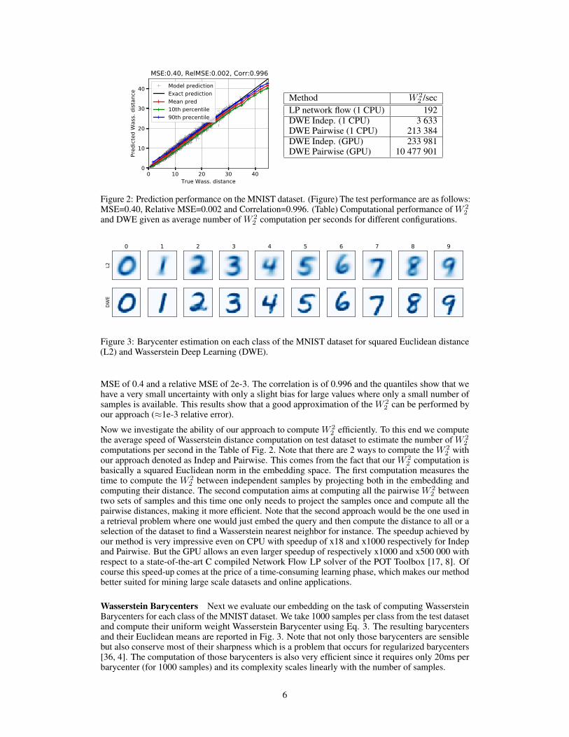
Numerical precision and computational performance The true and predicted values for theWasserstein distances are given in Fig. 2. We can see that we reach a good precision with a test

5

0 10 20 30 40True Wass. distance

0

10

20

30

40

Pred

icted

Was

s. di

stan

ce

MSE:0.40, RelMSE:0.002, Corr:0.996Model predictionExact predictionMean pred10th percentile90th precentile

Method W 22 /sec

LP network flow (1 CPU) 192DWE Indep. (1 CPU) 3 633DWE Pairwise (1 CPU) 213 384DWE Indep. (GPU) 233 981DWE Pairwise (GPU) 10 477 901

Figure 2: Prediction performance on the MNIST dataset. (Figure) The test performance are as follows:MSE=0.40, Relative MSE=0.002 and Correlation=0.996. (Table) Computational performance of W 2

2and DWE given as average number of W 2

2 computation per seconds for different configurations.

Figure 3: Barycenter estimation on each class of the MNIST dataset for squared Euclidean distance(L2) and Wasserstein Deep Learning (DWE).

MSE of 0.4 and a relative MSE of 2e-3. The correlation is of 0.996 and the quantiles show that wehave a very small uncertainty with only a slight bias for large values where only a small number ofsamples is available. This results show that a good approximation of the W 2

2 can be performed byour approach (≈1e-3 relative error).

Now we investigate the ability of our approach to compute W 22 efficiently. To this end we compute

the average speed of Wasserstein distance computation on test dataset to estimate the number of W 22

computations per second in the Table of Fig. 2. Note that there are 2 ways to compute the W 22 with

our approach denoted as Indep and Pairwise. This comes from the fact that our W 22 computation is

basically a squared Euclidean norm in the embedding space. The first computation measures thetime to compute the W 2

2 between independent samples by projecting both in the embedding andcomputing their distance. The second computation aims at computing all the pairwise W 2

2 betweentwo sets of samples and this time one only needs to project the samples once and compute all thepairwise distances, making it more efficient. Note that the second approach would be the one used ina retrieval problem where one would just embed the query and then compute the distance to all or aselection of the dataset to find a Wasserstein nearest neighbor for instance. The speedup achieved byour method is very impressive even on CPU with speedup of x18 and x1000 respectively for Indepand Pairwise. But the GPU allows an even larger speedup of respectively x1000 and x500 000 withrespect to a state-of-the-art C compiled Network Flow LP solver of the POT Toolbox [17, 8]. Ofcourse this speed-up comes at the price of a time-consuming learning phase, which makes our methodbetter suited for mining large scale datasets and online applications.

Wasserstein Barycenters Next we evaluate our embedding on the task of computing WassersteinBarycenters for each class of the MNIST dataset. We take 1000 samples per class from the test datasetand compute their uniform weight Wasserstein Barycenter using Eq. 3. The resulting barycentersand their Euclidean means are reported in Fig. 3. Note that not only those barycenters are sensiblebut also conserve most of their sharpness which is a problem that occurs for regularized barycenters[36, 4]. The computation of those barycenters is also very efficient since it requires only 20ms perbarycenter (for 1000 samples) and its complexity scales linearly with the number of samples.

6

Class 0 Class 1 Class 4L2 DWE L2 DWE L2 DWE

1 2 3 1 2 3 1 2 3 1 2 3 1 2 3 1 2 3

Figure 4: Principal Geodesic Analysis for classes 0,1 and 4 from the MNIST dataset for squaredEuclidean distance (L2) and Wasserstein Deep Learning (DWE). For each class and method we showthe variation from the barycenter along one of the first 3 principal modes of variation.

Principal Geodesic Analysis We report in Figure 4 the Principal Component Analysis (L2) andPrincipal Geodesic Analysis (DWE) for 3 classes of the MNIST dataset. We can see that usingWasserstein to encode the displacement of mass leads to more semantic and nonlinear subspacessuch as rotation/width of the stroke and global sizes of the digits. This is well known and has beenillustrated in [33]. Nevertheless our method allows for estimating the principal component evenin large scale datasets and our reconstruction seems to be more detailed compared to [33] maybebecause our approach can use a very large number of samples for subspace estimation.

4.3 Google doodle dataset

Datasets The Google Doodle dataset is a crowd sourced dataset that is freely available from theweb2 and contains 50 million drawings. The data has been collected by asking users to hand drawwith a mouse a given object or animal in less than 20 seconds. This lead to a large number ofexamples for each class but also a lot of noise in the sens that people often get stopped before the endof their drawing .We used the numpy bitmaps format proposed on the quick draw github account.Those are made of the simplified drawings rendered into 28x28 grayscale images. These images arealigned to the center of the drawing’s bounding box. In this paper we downloaded the classes Cat,Crab and Faces and tried to learn a Wasserstein embedding for each of these classes with the samearchitecture as used for MNIST. In order to create the training dataset we draw randomly 1 millionpairs of indexes from the training samples of each categories and compute the exact Wassersteindistance for quadratic ground metric using the POT toolbox [17]. Same as for MNIST, 700 000 areused for learning the neural network, 200 000 are used for validation and 100 000 pars are usedfor testing purposes. Each of the three categories( Cat, Crab and Faces) holds respectively 123202,126930 and 161666 training samples.

Numerical precision and cross dataset comparison The numerical performances of the learnedmodels on each of the doodle dataset is reported in the diagonal of Table 1. Those datasets are muchmore difficult than MNIST because they have not been curated and contain a very large variancedue to numerous unfinished doodles. An interesting comparison is the cross comparison betweendatasets where we use the embedding learned on one dataset to compute the W 2

2 on another. Thecross performances is given in Table 1 and shows that while there is definitively a loss in accuracyof the prediction, this loss is limited between the doodle datasets that all have an important variety.Performance loss across doodle and MNIST dataset is larger because the latter is highly structuredand one needs to have a representative dataset to generalize well which is not the case with MNIST.

2https://quickdraw.withgoogle.com/data

7

Network Data CAT CRAB FACE MNISTCAT 1.195 1.718 2.07 12.132

CRAB 2.621 0.854 3.158 10.881FACE 5.025 5.532 3.158 50.527

MNIST 9.118 6.643 4.68 0.405Table 1: Cross performance between the DWE embedding learned on each datasets. On each row,we observe the MSE of a given dataset obtained on the deep network learned on the four differentdatasets (Cat, Crab, Faces and MNIST).

Figure 5: Interpolation between four samples of each datasets using DWE. (left) cat dataset, (center)Crab dataset (right) Face dataset.

Wasserstein interpolation We first compute the Wasserstein interpolation between four samplesof each datasets in Figure 5. Note that these interpolation might not be optimal w.r.t. the objects butwe clearly see a continuous displacement of mass that is characteristic of optimal transport. Thisleads to surprising artefacts for example when the eye of a face fuse with the border while the noseturns into an eye. Also note that there is no reason for a Wasserstein barycenter to be a realisticsample.

Next we qualitatively evaluate the subspace learned by DWE by comparing the Wasserstein inter-polation of our approach with the true Wasserstein interpolation estimated by solving the OT linearprogram and by using regularized OT with Bregman projections [4]. The interpolation results for allthose methods and the Euclidean interpolation are available in Fig. 6. The LP solver takes a longtime (20 sec/interp) and leads to a “noisy” interpolation as already explained in [15]. The regularizedWasserstein barycenter is obtained more rapidly (4 sec/interp) but is also very smooth at the risk ofloosing some details, despite choosing a small regularization that prevents numerical problems. Ourreconstruction also looses some details due to the Auto-Encoder error but is very fast and can be donein real time (4 ms/interp).

5 Conclusion and discussion

In this work we presented a computational approximation of the Wasserstein distance suitable forlarge scale data mining tasks. Our method finds an embedding of the samples in a space where theEuclidean distance emulates the behavior of the Wasserstein distance. Thanks to this embedding,numerous data analysis tasks can be conducted at a very cheap computational price. We forecast thatthis strategy can help in generalizing the use of Wasserstein distance in numerous applications.

However, while our method is very appealing in practice it still raises a few questions about thetheoretical guarantees and approximation quality. First it is difficult to foresee from a given networkarchitecture if it is sufficiently (or too much) complex for finding a successful embedding. It canbe conjectured that it is dependent on the complexity of the data at hand and also the locality ofthe manifold where the data live in. Second, the theoretical existence results on such Wassersteinembedding with constant distortion are still lacking. Future works will consider these questions aswell as applications of our approximation strategy on a wider range of ground loss and data mining

8

Figure 6: Comparison of the interpolation with L2 Euclidean distance (top), LP Wasserstein interpo-lation (top middle) regularized Wasserstein Barycenter (down middle) and DWE (down).

tasks. Also, we will study the transferability of one database to another to diminish the computationalburden of computing Wasserstein distances on numerous pairs for the learning process.

References[1] M. Agueh and G. Carlier. Barycenters in the wasserstein space. SIAM Journal on Mathematical Analysis,

43(2):904–924, 2011.

[2] A. Andoni, A. Naor, and O. Neiman. Impossibility of Sketching of the 3D Transportation Metric withQuadratic Cost. In 43rd International Colloquium on Automata, Languages, and Programming (ICALP2016), volume 55, pages 83:1–83:14, 2016.

[3] M. Arjovsky, S. Chintala, and L. Bottou. Wasserstein generative adversarial networks. In Proceedings ofthe 34th International Conference on Machine Learning, volume 70, pages 214–223, Sydney, Australia,06–11 Aug 2017.

[4] J.-D. Benamou, G. Carlier, M. Cuturi, L. Nenna, and G. Peyré. Iterative Bregman projections for regularizedtransportation problems. SISC, 2015.

[5] J. Bigot, R. Gouet, T. Klein, A. López, et al. Geodesic pca in the wasserstein space by convex pca. InAnnales de l’Institut Henri Poincaré, Probabilités et Statistiques, volume 53, pages 1–26. Institut HenriPoincaré, 2017.

[6] N. Bonneel, G. Peyré, and M. Cuturi. Wasserstein barycentric coordinates: Histogram regression usingoptimal transport. ACM Trans. Graph., 35(4):71:1–71:10, July 2016.

[7] N. Bonneel, J. Rabin, G. Peyré, and H. Pfister. Sliced and radon wasserstein barycenters of measures.Journal of Mathematical Imaging and Vision, 51(1):22–45, Jan 2015.

[8] N. Bonneel, M. van de Panne, S. Paris, and W. Heidrich. Displacement interpolation using Lagrangianmass transport. ACM Transaction on Graphics, 30(6), 2011.

[9] J. Bromley, I. Guyon, Y. LeCun, E. Säckinger, and R. Shah. Signature verification using a" siamese" timedelay neural network. In Advances in Neural Information Processing Systems, pages 737–744, 1994.

[10] M. Charikar. Similarity estimation techniques from rounding algorithms. In Proceedings of the Thiry-fourthAnnual ACM Symposium on Theory of Computing, STOC ’02, pages 380–388, 2002.

[11] S. Chopra, R. Hadsell, and Y. LeCun. Learning a similarity metric discriminatively, with application toface verification. In Computer Vision and Pattern Recognition, 2005. CVPR 2005. IEEE Computer SocietyConference on, volume 1, pages 539–546. IEEE, 2005.

[12] N. Courty, R. Flamary, D. Tuia, and A. Rakotomamonjy. Optimal transport for domain adaptation. IEEETransactions on Pattern Analysis and Machine Intelligence, 2017.

[13] M. Cuturi. Sinkhorn distances: Lightspeed computation of optimal transportation. In Advances on NeuralInformation Processing Systems (NIPS), pages 2292–2300, 2013.

[14] M. Cuturi and A. Doucet. Fast computation of Wasserstein barycenters. In ICML, 2014.

[15] M. Cuturi and G. Peyré. A smoothed dual approach for variational wasserstein problems. SIAM Journalon Imaging Sciences, 9(1):320–343, 2016.

[16] F. de Goes, K. Breeden, V. Ostromoukhov, and M. Desbrun. Blue noise through optimal transport. ACMTrans. Graph., 31(6):171:1–171:11, Nov. 2012.

[17] R. Flamary and N. Courty. Pot python optimal transport library. 2017.

9

[18] P. T. Fletcher, C. Lu, S. M. Pizer, and S. Joshi. Principal geodesic analysis for the study of nonlinearstatistics of shape. IEEE Trans. Medical Imaging, 23(8):995–1005, Aug. 2004.

[19] G. Gasso, A. Rakotomamonjy, and S. Canu. Recovering sparse signals with a certain family of nonconvexpenalties and dc programming. IEEE Transactions on Signal Processing, 57(12):4686–4698, 2009.

[20] A. Genevay, M. Cuturi, G. Peyré, and F. Bach. Stochastic optimization for large-scale optimal transport. InNIPS, pages 3432–3440, 2016.

[21] G. Huang, C. Guo, M. Kusner, Y. Sun, F. Sha, and K. Weinberger. Supervised word mover’s distance. InAdvances in Neural Information Processing Systems, pages 4862–4870, 2016.

[22] P. Indyk and N. Thaper. Fast image retrieval via embeddings. In 3rd International Workshop on Statisticaland Computational Theories of Vision, pages 1–15, 2003.

[23] S. Khot and A. Naor. Nonembeddability theorems via fourier analysis. Mathematische Annalen, 334(4):821–852, Apr 2006.

[24] G. Koch, R. Zemel, and R. Salakhutdinov. Siamese neural networks for one-shot image recognition. InICML Deep Learning Workshop, volume 2, 2015.

[25] S. Kolouri, S. R. Park, and G. K. Rohde. The radon cumulative distribution transform and its application toimage classification. IEEE Transactions on Image Processing, 25(2):920–934, 2016.

[26] S. Kolouri, S. R. Park, M. Thorpe, D. Slepcev, and G. K. Rohde. Optimal mass transport: Signal processingand machine-learning applications. IEEE Signal Processing Magazine, 34(4):43–59, July 2017.

[27] S. Kolouri, A. Tosun, J. Ozolek, and G. Rohde. A continuous linear optimal transport approach for patternanalysis in image datasets. Pattern Recognition, 51:453 – 462, 2016.

[28] S. Kolouri, Y. Zou, and G. Rohde. Sliced wasserstein kernels for probability distributions. 2016 IEEEConference on Computer Vision and Pattern Recognition (CVPR), pages 5258–5267, 2016.

[29] J. Matoušek. Lecture notes on metric embeddings. Technical report, ETH Zurich, 2013.

[30] J. Matoušek and A. Naor. Open problems on embeddings of finite metric spaces. available at http://kam.mff.cuni.cz/~matousek/metrop.ps, 2011.

[31] A. Rolet, M. Cuturi, and G. Peyré. Fast dictionary learning with a smoothed wasserstein loss. In AISTATS,pages 630–638, 2016.

[32] F. Santambrogio. Introduction to optimal transport theory. Notes, 2014.

[33] V. Seguy and M. Cuturi. Principal geodesic analysis for probability measures under the optimal transportmetric. In Advances in Neural Information Processing Systems, pages 3312–3320, 2015.

[34] S. Shirdhonkar and D. W. Jacobs. Approximate earth mover’s distance in linear time. In CVPR, pages 1 –8, June 2008.

[35] J. Solomon, F. de Goes, G. Peyré, M. Cuturi, A. Butscher, A. Nguyen, T. Du, and L. Guibas. Convolutionalwasserstein distances: Efficient optimal transportation on geometric domains. ACM Trans. Graph.,34(4):66:1–66:11, July 2015.

[36] J. Solomon, F. De Goes, G. Peyré, M. Cuturi, A. Butscher, A. Nguyen, T. Du, and L. Guibas. Convolutionalwasserstein distances: Efficient optimal transportation on geometric domains. ACM Transactions onGraphics (TOG), 34(4):66, 2015.

[37] M. Staib, S. Claici, J. Solomon, and S. Jegelka. Parallel streaming wasserstein barycenters. CoRR,abs/1705.07443, 2017.

[38] C. Villani. Optimal transport: old and new. Grund. der mathematischen Wissenschaften. Springer, 2009.

[39] W. Wang, D. Slepcev, S. Basu, J. Ozolek, and G. Rohde. A linear optimal transportation frameworkfor quantifying and visualizing variations in sets of images. International Journal of Computer Vision,101(2):254–269, Jan 2013.

[40] J. Weston, F. Ratle, H. Mobahi, and R. Collobert. Deep learning via semi-supervised embedding. In NeuralNetworks: Tricks of the Trade, pages 639–655. Springer, 2012.

[41] C. Wu and E. Tabak. Statistical archetypal analysis. arXiv preprint arXiv:1701.08916, 2017.

[42] W. Yu, G. Zeng, P. Luo, F. Zhuang, Q. He, and Z. Shi. Embedding with autoencoder regularization. InECML/PKDD, pages 208–223. Springer, 2013.

10