Methods for Validation of a Turbomachinery Rotor Blade Tip Timing System

Todd M. Pickering

Thesis submitted to the faculty of the Virginia Polytechnic Institute and State University

in partial fulfillment of the requirements for the degree of

Master of Science In

Mechanical Engineering

Walter F. O’Brien, Chair Robert L. West Alfred L. Wicks

March 4, 2014 Blacksburg, Virginia

Keywords: Blade Tip Timing, Non-Intrusive Stress Measurement System, Turbomachinery, Optical Sensor, Piezoelectric

Copyright 2014, Todd M. Pickering

Methods for Validation of a Turbomachinery Rotor Blade Tip Timing System

Todd M. Pickering

ABSTRACT This research developed two innovative test methods that were used to experimentally evaluate the performance of a novel blade tip timing (BTT) system from Prime Photonics, LC. The research focused on creating known blade tip offsets and tip vibrations so that the results from a BTT system can be validated. The topic of validation is important to the BTT field as the results between many commercial systems still are not consistent. While the system that was tested is still in development and final validation is not complete, the blade tip offset and vibration frequency validation results show that this BTT system will be a valuable addition to turbomachinery research and development programs once completed. For the first test method custom rotors were created with specified blade tip offsets. For the blade tip offset alternate measurement, the rotors were optically scanned and analyzed in CAD software with a tip location uncertainty of 0.1 mm. The BTT system agreed with the scanned results to within 0.13 mm. Tests were also conducted to ensure that the BTT system identified and indexed the blades properly. The second developed test method used an instrumented piezoelectric blade to create known dynamic deflections. The active vibration rotor was able to create measureable deflection over a range of frequencies centered on the first bending mode of the blade. The results for the 110 Hz, 150 Hz, 180 Hz first bending resonance, 200 Hz, and 1036 Hz second bending resonance cases are presented. A strain gage and piezoelectric sensor were attached to the active blade during the dynamic deflection tests to provide an alternate method for determining blade vibration frequency. The BTT system correctly identified the active blade excitation frequencies as well as a 120 Hz frequency from the drive motor. This thesis also explored applying BTT methods and testing to more realistic blade geometry and vibration. Blade vibrations are usually classified by their frequency relative to the rotation speed. Synchronous vibrations are integer multiples of the rotational speed and are often excited by struts or vanes fixed to the engine case. For this reason, special probe placement algorithms were explored that use sine curve fitting to optimize the probe placement. Knowing how the blade will vibrate at operation before testing is critical as well. In preparation for future research, ANSYS Mechanical was used to predict the first three modes of a PT6A-28 first stage rotor blade at 1,966, 5,539, and 7,144 Hz. These frequencies were validated to within 4% using scanning laser vibrometry. The simulation was repeated at speed to produce a Campbell Diagram to highlight synchronous excitation crossings.

iii

Acknowledgments I first would like to thank everyone at Prime Photonics for their technical and financial support of this project. The blade tip timing system evaluated in this thesis is the result of many years of their hard work. In particular I would like to thank Dan Kominsky, Malcolm Laing, Chris Westcott, Jonathan Sides and Steve Poland for their direction and patience on both this research and the earlier high temperature clearance testing project. Without their and everyone at Prime Photonics help this project would not have been possible. Additional support for the project was supplied by Dr. Norris Lewis from Moog Components Group in the form of two ten-conductor slip rings supplied at no cost to the project. This device allowed for direct vibration measurements to be taken while the rotor was spinning, one of the key aspects of this research. I also wish to thank the three members of my committee: Dr. Walter O’Brien, Dr. Robert West and Dr. Alfred Wicks. Your advice on this project as well as your classes in turbomachinery, finite element analysis, and instrumentation were invaluable to this research and my future career. The best part of graduate school was the people that I was privileged to work with at the Virginia Tech Turbomachinery and Propulsion Research Laboratory: Dr. Walter O’Brien, Tony Ferrar, Bill Schneck, Justin Bailey, Kevin Hoopes, James Lucas, Chaitanya Halbe, Steven Steele, Chris Collins, Gregg Perley and Bill Bryant. Thank you for all of your help with my project and for sharing the fun, challenge, and knowledge gained from your projects during my years here. Your willingness to teach, to guide, and to explore are what made my graduate degree so much more than just two more years of college. Also an extra thanks to Bill and Justin for the excessive number of hours we spent many weeks discussing Star Trek at the office. I would also like to thank my family, for without their support and occasional prodding I would never have completed this thesis or have been inspired to push the limits of my education in the first place. In particular I would like to thank my brother, Brent Pickering, for always being there for me and acting as a sounding board when I most needed it. And finally I wish to thank my parents, Ray and Jayne Pickering, for their unwavering support while holding me to the high standards that I expect of myself today. Photos not cited are by the author.

iv

Contents Chapter 1: Introduction and Background ......................................................................... 1

Chapter 2: Literature Review ........................................................................................... 3

2.1 Introduction ......................................................................................................... 3

2.2 Need for Blade Tip Timing and Health Monitoring .............................................. 3

2.3 Blade Tip Timing in Research and Industry ......................................................... 5

2.3.1 Development ................................................................................................. 6

2.3.2 Application ................................................................................................... 6

2.4 Exciting Blade Resonances for Validation Testing ............................................... 8

2.4.1 Synchronous Excitations ............................................................................... 9

2.4.2 Asynchronous Excitations ........................................................................... 10

2.5 Testing Application Detail - Foreign Object Damage ......................................... 11

2.5.1 In-Service Engine Observation .................................................................... 12

2.5.2 FOD Simulated for Research ....................................................................... 13

2.6 Summary and Introduction to the Present Research ............................................ 14

Chapter 3: Fundamental Blade Tip Timing Methods ...................................................... 15

3.1 Introduction ....................................................................................................... 15

3.2 Determining Blade Time of Arrival ................................................................... 16

3.3 Converting Time of Arrival to Blade Deflection ................................................ 18

3.4 Optimizing Timing Probe Placement ................................................................. 21

3.5 Predicting Vibration Mode Frequencies ............................................................. 24

3.6 Summary of Vibration Frequency Extraction Methods ....................................... 28

Chapter 4: Direct Vibration Measurement Tools for Blade Tip Timing Validation......... 30

4.1 Introduction ....................................................................................................... 30

4.2 Blade Deflection Measurement Using Strain Gages ........................................... 30

4.2.1 General Methods ......................................................................................... 30

4.2.2 Application to Current Research.................................................................. 31

4.3 Blade Vibration Measurement Using Piezoelectric Sensors ................................ 33

4.3.1 General Methods ......................................................................................... 33

4.3.2 Application to Current Research.................................................................. 33

4.4 Signal Transfer Using Slip Rings ....................................................................... 34

Chapter 5: Validation I Methods and Testing – Blade and Probe Static Offset ............... 36

v

5.1 Introduction ....................................................................................................... 36

5.2 Machined Blade Offset Rotors ........................................................................... 36

5.2.1 Design and TOA Measurement ................................................................... 37

5.2.2 Measuring Blade Offset for Tip Timing Result Validation .......................... 41

5.3 Blade Indexing Validation ................................................................................. 43

5.4 Probe Location Offset ........................................................................................ 45

Chapter 6: Validation II Methods - Exciting Dynamic Deflections ................................ 47

6.1 Introduction ....................................................................................................... 47

6.2 Exciting Synchronous Vibrations ....................................................................... 47

6.3 Exciting Asynchronous Vibrations ..................................................................... 50

Chapter 7: Validation II Testing - Dynamic Deflection .................................................. 51

7.1 Introduction ....................................................................................................... 51

7.2 Active Vibration Excitation Rotor Spin Rig ....................................................... 51

7.2.1 Spin Rig and Drive Design and Construction .............................................. 51

7.2.2 Active Rotor Design and Construction ........................................................ 55

7.3 Asynchronous Vibration Frequency Testing....................................................... 59

7.4 Methods to Increase Spin Rig Capabilities ......................................................... 65

Chapter 8: Discussion of Results ................................................................................... 67

8.1 Introduction ....................................................................................................... 67

8.2 Methods of Blade Vibration Measurements........................................................ 67

8.3 Static Offset Testing .......................................................................................... 68

8.4 Dynamic Deflection Testing .............................................................................. 68

Chapter 9: Conclusions and Recommendations ............................................................. 70

9.1 Conclusions ....................................................................................................... 70

9.2 Recommendations.............................................................................................. 71

Bibliography ................................................................................................................. 72

Appendix A: Selecting the Time of Arrival Method....................................................... 75

Appendix B: Curve Fitting to Extract Frequency and Amplitude ................................... 78

vi

List of Figures Figure 1. Class A and B Engine Related Mishap Costs by Component. B. Stange, "ISA Standards for Turbine Engine Test Cell Instrumentation," ISA, Wyndham Hotel, Cleveland, 2012. Public Domain .................................................................................... 4 Figure 2. Rotating Instability Vortex that can cause asynchronous vibrations and HCF. C. Hah, "Flow Instabilities and Non-Synchronous Vibration in a Compressor," in 8th ISAIF, Lyon, 2007. Public Domain ................................................................................ 5 Figure 3. Campbell Diagram for NPS BTT rotor results and NASA predictions. The orange, blue and beige data points overlay the NASA predition of blade natural frequency (red line). W. P. Murphy, "High-Speed Blade Vibration in a Transonic Compressor," Monterey, 2008. Public Domain ..................................................................................... 7 Figure 4. Left: Sample eddy current sensor data for a single blade passage with left and right lobe threshold width noted. Right: When the onset of stall is near, the variance of the threshold width ratio changes. C. Teolis, D. Gent, C. Kim, A. Teolis, J. Paduano and M. Bright, "Eddy Current Sensor Signal Processing for Stall Detection," IEEEAC, vol. Paper #1255, 2005. Used under fair use, 2014 ................................................................ 8 Figure 5. 8 upstream blockages excited both 8 EO (2nd bending) and 2 EO (1st bending) blade vibrations. J. Gallego-Garrido, G. Dimitriadis, I. B. Carrington and J. R.Wright, "A Class ofMethods for the Analysis of Blade Tip Timing Data from Bladed Assemblies Undergoing Simultaneous Resonances—Part II: Experimental Validation," International Journal of Rotating Machinery, p. Article ID 73624, 2007. Used under fair use, 2014 .... 9 Figure 6. Magnet final position for optimal blade synchronous excitation. M. R. Mansisidor, "Resonant Blade Response in Turbine Rotor Spin Tests using a Laser-Light Probe Non-Intrusive Measurement System," Monterey, 2002. Public Domain .............. 10 Figure 7. Piezoelectric film actuators mounted to the face of spin rig compressor blades. I. Goltz, H. Böhmer, R. Nollau, J. Belz, B. Grueber and J. Seume, "Piezo-Electric Actuation of Rotor Blades in an Axial Compressor". Used under fair use, 2014............ 11 Figure 8. Small notch in a Garrett F109 fan blade caused by impact with foreign object 11 Figure 9. Distribution and severity of FOD on 10 randomly selected F404 engine (F18) first stage fan blades. P. Prevéy, D. Hornbach, J. Cammett and R. Ravindranath, "Damage Tolerance Improvement of Ti-6-4 Fan Blades with Low Plasticity Burnishing," in 6th Joint FAA/DoD/NASA Aging Aircraft Conference, 2002. Used under fair use, 2014 .............................................................................................................................. 12

vii

Figure 10. Failed HPC blade due to continued operation after impact with a rivet head. G. Morse, "Analysis of Engine Damage - Engine SN 451-133," Failure Analysis Service Technology, Inc, 2007. Used under fair use, 2014 ........................................................ 13 Figure 11. View of head on impact of spherical projectile strike on simulated airfoil. J. J. Ruschau, T. Nicholas and S. R. Thompson, "Influence of foreign object damage (FOD) on the fatigue life of simulated Ti-6Al-4V airfoils," International Journal of Impact Engineering, vol. 25, pp. 233-250, 2001. Used under fair use, 2014 .............................. 13 Figure 12. Example TOA points on a blade tip scan. (1) Rise Start, (2) Threshold, (3) Fall End ............................................................................................................................... 16 Figure 13. Example actual blade tip scans that can create noisy data with some TOA algorithms ..................................................................................................................... 17 Figure 14. Image of actual used blade tip from the Virginia Tech Turbomachinery and Propulsion Research Laboratory JT15D. Note the bright pressure and suction edges and dark center of the blade tip ............................................................................................ 17 Figure 15. The ideal blade TOA are used as the reference for the actual blade TOA offset which is used as the reference for determining blade vibratory deflection ...................... 19 Figure 16. Stack Plot with simulated data for the average result from 8 probes on a 17 blade rotor ..................................................................................................................... 20 Figure 17. Actual blade deflection distribution data over 500 rotations from a single probe on a 12 blade rotor with blade 1 (bottom) resonating............................................ 21 Figure 18. Incorrect probe spacing can lead to no vibration observed for a synchronous event or aliasing if the probes are too widely spaced. The stars mark the measurement points and the dashed line is the sine curve fit................................................................ 22 Figure 19. PT6A-28 first stage compressor rotor as received from overhaul shop, Airforce Turbine Service ............................................................................................................. 24 Figure 20. PT6A-28 hardware scanned and 3D modeled for FE analysis, GKS Laser Design ........................................................................................................................... 24 Figure 21. Final refined PT6A-28 Blade FE mesh ......................................................... 26 Figure 22. 3rd Mode frequency mesh convergence plot. The finest refinement (100k elements) was selected for the analysis .......................................................................... 26 Figure 23. The first three mode shapes and frequencies for the PT6A-28 blade from an ANSYS Mechanical modal analysis. Red is motion out of the page, blue is motion into the page, and green is stationary .................................................................................... 27

viii

Figure 24. The experimental mode shape results from laser vibrometry scan of the blades. Red is motion out of the page, blue is motion into the page, and green is stationary ....... 28 Figure 25. Strain field from FE analysis of a PT6A-28 blade at first bending mode from the ANSYS Mechanical modal analysis ......................................................................... 31 Figure 26. The test configuration for the strain gage on blade vibration measurements .. 32 Figure 27. Omega DMD-465WB strain gage amplification and filtering circuit. Omega Engineering Inc., "DMD-465WB Bridgesensor AC Powered Signal Conditioner," 1999. Used under fair use, 2014 .............................................................................................. 32 Figure 28. The piezoelectric sensor system required only the sensor connected to the oscilloscope through the slip ring .................................................................................. 33 Figure 29. Schematic of a four conductor wire brush slip ring ....................................... 34 Figure 30. Moog EC3848 10,000 RPM 10 circuit high speed slip ring ........................... 35 Figure 31. High speed router spin rig that was used for the static offset testing .............. 37 Figure 32. A CAD model for a 24 blade paddlewheel blisk ........................................... 38 Figure 33. Offsets for 36 blade sine wave paddlewheel blisk ......................................... 38 Figure 34. Blade deflection distribution plot from 275 rotations of the sine wave rotor using an unlensed probe ................................................................................................ 39 Figure 35. Mean blade offsets for sine wave rotor.......................................................... 40 Figure 36. Blade deflection distribution plot from 197 rotations of the 50 blade uniform blade spacing blisk using an unlensed probe .................................................................. 40 Figure 37. Mean blade offsets for 50 blade uniform spacing blisk with unlensed probe . 41 Figure 38. Static deflections for 36 blade sine wave paddlewheel blisk. ......................... 41 Figure 39. Blade offset for the sine wave rotor from optical scanning and BTT using an unlensed probe .............................................................................................................. 42 Figure 40. Blade offset for the uniform rotor from optical scanning and BTT using an unlensed probe .............................................................................................................. 43 Figure 41. By using an offset pattern with a sharp discontinuity, the blade 1 identification by a BTT system can be verified.................................................................................... 44

ix

Figure 42. Saw tooth plastic rotor for blade 1 identification testing ................................ 44 Figure 43. Blade deflection distribution plot for the saw tooth offset rotor. The jump in offset amplitude (from positive to negative) should occur at blade 1, which it does ....... 45 Figure 44. The EO lines show what frequencies will be excited for various EO excitations with rotor speed. For a rotor operational speed of 0 to 20,000 RPM and 1 to 15 EO excitations ..................................................................................................................... 48 Figure 45. Complete Campbell diagram of PT6 blade first three modes with example 5EO crossing at 2,125 Hz and 25,500 RPM ................................................................... 49 Figure 46. Due to the opposite orientation of the piezoelectric plates one plate contracts while the other expands when a voltage is applied to the bimorph actuator, causing the device to bend ............................................................................................................... 50 Figure 47. CAD Model of new HCF Rig ....................................................................... 52 Figure 48. Construction of new HCF Rig....................................................................... 52 Figure 49. Acquired Piezoelectric Bending (Bimorph) Actuator .................................... 53 Figure 50. Active Rotor Design (12 piezoelectric bimorph blades shown) ..................... 53 Figure 51. Piezoelectric power supply and mounted bimorph actuator ........................... 54 Figure 52. Model of slip ring mounted in new spin rig ................................................... 54 Figure 53. Active rotor, slip ring, and OPR sensor system assembled ............................ 55 Figure 54. Detail view of active blade with attached and wired strain gage .................... 55 Figure 55. Voltage created by passive piezoelectric blade, recorded while spinning ....... 56 Figure 56. The (a) first bending, (b) second bending, and (c) first torsion modes for the piezoelectric active blade ............................................................................................... 57 Figure 57. The (a) first bending, (b) second bending, and (c) first torsion modes for the aluminum plate blades ................................................................................................... 57 Figure 58. A harmonic sweep of the active blade showing a clear first bending mode and a spread second bending mode ...................................................................................... 58 Figure 59. Active blade at first bending resonance, 175 Hz ............................................ 58

x

Figure 60. Piezoelectric sensor and strain gages mounted to active (piezoelectric) blade 59 Figure 61. Time and frequency domain strain gage signal for active blade rotating at 2200RPM while resonating at 180 Hz ........................................................................... 60 Figure 62. Switching the piezoelectric voltage from 0V (Left) to 100V (Right), the BTT system reported a static offset change of 0.5 mm. The left scale in both figures is in millimeters .................................................................................................................... 60 Figure 63. Active rotor sweep from 1500 RPM to 2500 RPM and resonating at 180 Hz, FFT from piezoelectric sensor compared with spectral analysis of blade tip timing data. Note that the tip timing magnitude is in dB while the strain gage is in raw voltage ........ 61 Figure 64. The 120Hz motor vibration causes a strong vibration on all blades, while the 180Hz piezoelectric vibration is highest on the active blade .......................................... 62 Figure 65. The active blade excited at 110 Hz................................................................ 63 Figure 66. The active blade excited at 150 Hz................................................................ 63 Figure 67. The active blade excited at 200 Hz................................................................ 63 Figure 68. All blades with no active blade excitation ..................................................... 64 Figure 69. Detail View of all blade response with 110 Hz active blade excitation .......... 64 Figure 70. Active blade with 1036 Hz excitation resulting in second bending resonance 65 Figure 71. PT6 blade velocity triangles at 10,000 RPM – β1 and β2 were approximated from the CAD model of the blade .................................................................................. 65 Figure 72. Great optical blade reflectivity profile on blade 23 from JT15D testing ......... 76 Figure 73. Poor falling edge optical reflectivity profile on blade 3 from JT15D testing .. 76 Figure 74. Optical reflectivity profile of the tip of the active blade ................................ 78 Figure 75. Deflection (mm) vs. time (s) for the active blade with deflection data from all probes combined ........................................................................................................... 79 Figure 76. Example method for converting individual probe blade TOA data to combined blade deflection data ...................................................................................................... 79 Figure 77. Raw strain gage signal as captured by the oscilloscope while the rotor was spinning at 1650 RPM ................................................................................................... 80

xi

Figure 78. FFT of the strain gage data indicating significant deflection amplitude at 180 Hz and 120 Hz............................................................................................................... 80 Figure 79. Two component sine wave least squares fit (red dashed line) to BTT data (blue)............................................................................................................................. 82

xii

List of Tables Table 1. Material properties of PT6 blade and possible blade materials.......................... 25 Table 2. FE and experimental vibration mode frequency summary ................................ 28 Table 3. Correction of probe locations using TOA data over 100 rotor revolutions ........ 46 Table 4. Timing Resolution for blade 3, blade 23, and all blades ................................... 77 Table 5. Final coefficients for non-linear least squares fit of 58 points of BTT data ....... 81

xiii

Nomenclature AFRL Air Force Research Laboratory BHM Blade Health Monitoring Blisk Bladed Disk BTT Blade Tip Timing CFD Computational Fluid Dynamics EO Engine Order FE Finite Element FFT Fast Fourier Transform FOD Foreign Object Damage HCF High Cycle Fatigue HPC High Pressure Compressor Kulite High Response Pressure Transducer NPS Navy Postgraduate School NSMS Non-intrusive Stress Measurement System OPR Once Per Revolution sensor TOA Time of Arrival USAF United States Air Force USN United States Navy

1

Chapter 1: Introduction and Background Modern aerospace propulsion turbomachinery blades are designed to operate under extreme stress and variable loading conditions safely over a long hardware life. To achieve this, extensive testing is completed during development using both strain gages and blade tip timing (BTT) systems to ensure that the operational blade vibrations are safe and predictable for the desired life of the engine. In the development stage, higher accuracy and flexibility are desired of BTT systems. Once an engine design is put into service, problems often arise that were not encountered during ground engine testing. Fouling, modifications, material aging, and foreign object damage (FOD) can lead to blade strength reduction or unexpected blade vibrations that can significantly reduce the life of the blades or lead to catastrophic failure. For this reason in-service blade health monitoring (BHM) that can alert the operator of unsafe conditions is desired. Flight health monitoring systems must also be lightweight and durable to fouling and vibration. Damage to turbomachinery rotor blades from the ingestion of foreign objects, design and material flaws, or in-service modifications can lead to costly and catastrophic failures in both aircraft and surface based turbomachines. Detecting unexpected or excessive blade vibration before failure is critical to ensure safety and to achieve expected equipment life. Traditional detection methods have relied solely on component inspection once the turbomachine is in-service and strain gage telemetry systems during design. Both of these methods require time consuming and costly modifications of the turbomachine and cannot provide robust feedback of health when in operation. In recent decades a third method has begun to become widely used. BTT with various software packages is the basis for the several NSMS (non-intrusive stress measurement system) in present use. BTT uses sensors arranged around the rotor to precisely determine the time of arrival (TOA) of each blade tip at each sensor. This data is then used in conjunction with a once per revolution (OPR) sensor located on the shaft of the turbomachine to compute blade tip TOA lead and lag which is a measure of tip deflection. The deflection measurements are not continuous as they can only be made at BTT probe locations. Due to this limitation, extensive sensor and algorithm performance evaluation and result validation is required before a BTT system can be used for blade stress or health monitoring. The goal of this thesis was to design and carry out the first set of comprehensive evaluation tests on an optical BTT system in development by a commercial organization, and to use the results to plan final system validation testing. The thesis reports the development of two innovative BTT testing and validation methods, and experimental results of the evaluation of a novel BTT system. The BTT sensors and analysis system were developed by Prime Photonics, LC. The testing was completed using purpose-built spin rigs installed at the Prime Photonics laboratory located in Blacksburg, Virginia. The goal of the testing was to aid in the development of the BTT system and to validate the system performance. Once complete the system will

2

become a valuable tool to the aerospace propulsion industry, the military, and to future Virginia Tech turbomachinery research. To provide an introduction to this field, the Literature Review in Chapter 2 will focus on recent research and methods in the fields of BTT and NSMS. The primary focus will be on validation of NSMS systems as well as detecting FOD or high cycle fatigue (HCF) using them. Following the review, the fundamentals of BTT analysis and probe placement will be explored in Chapter 3. As one of the goals of this research is to validate the BTT system, Chapter 4 will explore alternative blade vibration measurement methods. The testing portion of this thesis will be split into two main sections, with blade tip static offset validation covered in Chapter 5, and the design and operation of a dynamic deflection test rig in Chapters 6 and 7. Finally, this report will conclude with a discussion of results in Chapters 8 and 9, as well as how to continue and expand this research.

3

Chapter 2: Literature Review

2.1 Introduction When developing a new technology, the key to success is to determine the requirements of the potential customers so that the optimum implementation goals can be set. For BTT there are two distinct fields: engine development and in-service health monitoring. In engine development the primary goal is to confirm that the blades are responding as predicted and that stress profiles correlate well to FE models. In-service health monitoring focuses on detecting and identifying unexpected events such as aeroelastic excitation or FOD. Both of these fields would benefit from the development of a BTT system with higher accuracy and more robust components. The actual current state of the art in BTT is difficult to determine as much of the development is internal or proprietary. Due to this, government and industry funded university research and conference proceedings are often the best source of information on the topic. Current published works in the field can generally be split into two groups: development and validation of BTT methods and usage of BTT systems to supplement or replace strain gages for a research test. Both of these topics can provide valuable insight into current BTT requirements.

2.2 Need for Blade Tip Timing and Health Monitoring Modern aircraft blades and bladed disks (Blisks) undergo significant computational simulation and physical testing before they are approved to enter service. During this testing the components are pushed beyond their rated performance and life to ensure that they will survive for the design life. In an ideal world this would be all that is necessary. However, in the industry today extensive regular inspections and early overhauls are implemented and problems are still missed that can lead to expensive and possibly deadly mishaps. A BHM system can not only alert an operator of an impending failure, but also reduce inspection frequency and increase rated component life. This technology would be useful to all gas turbine and turbomachinery system operators. One such customer that would benefit from a BHM system is the United States Air Force (USAF). They expect high performance levels and regularly push their engines and aircraft up to the design limits. On average, they observe that nearly 60% of their regular maintenance costs are directed at the rotating components of their engines. Unfortunately, even with this high maintenance allocation, failures or mishaps can occur. Mishaps are categorized based on severity; Class A is the most severe at 2 million dollars or more in damage or a fatality or permanent total disability. Class B is from 500,000 to 2 million dollars or a permanent partial disability or hospitalization of 5 or more personnel. In the fiscal years from 1993 to 2004, three of the top four most expensive causes of Class A and Class B mishaps originated in the bladed components of the engine

4

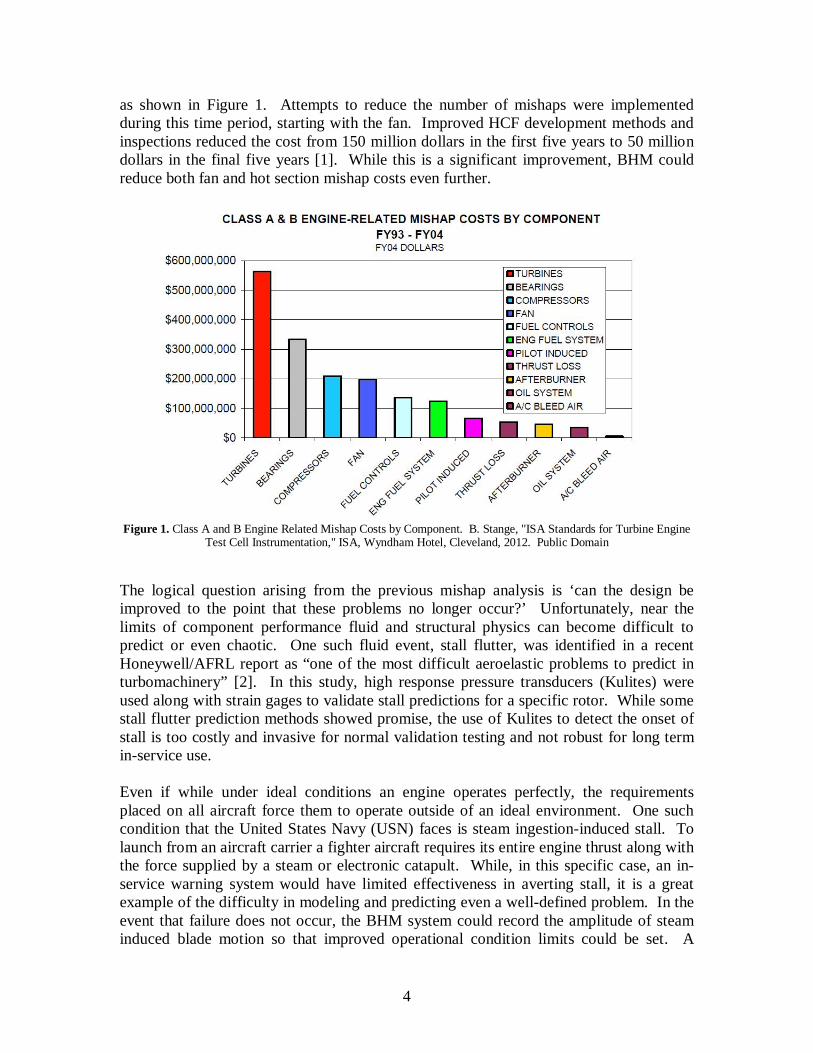
as shown in Figure 1. Attempts to reduce the number of mishaps were implemented during this time period, starting with the fan. Improved HCF development methods and inspections reduced the cost from 150 million dollars in the first five years to 50 million dollars in the final five years [1]. While this is a significant improvement, BHM could reduce both fan and hot section mishap costs even further.

Figure 1. Class A and B Engine Related Mishap Costs by Component. B. Stange, "ISA Standards for Turbine Engine

Test Cell Instrumentation," ISA, Wyndham Hotel, Cleveland, 2012. Public Domain

The logical question arising from the previous mishap analysis is ‘can the design be improved to the point that these problems no longer occur?’ Unfortunately, near the limits of component performance fluid and structural physics can become difficult to predict or even chaotic. One such fluid event, stall flutter, was identified in a recent Honeywell/AFRL report as “one of the most difficult aeroelastic problems to predict in turbomachinery” [2]. In this study, high response pressure transducers (Kulites) were used along with strain gages to validate stall predictions for a specific rotor. While some stall flutter prediction methods showed promise, the use of Kulites to detect the onset of stall is too costly and invasive for normal validation testing and not robust for long term in-service use. Even if while under ideal conditions an engine operates perfectly, the requirements placed on all aircraft force them to operate outside of an ideal environment. One such condition that the United States Navy (USN) faces is steam ingestion-induced stall. To launch from an aircraft carrier a fighter aircraft requires its entire engine thrust along with the force supplied by a steam or electronic catapult. While, in this specific case, an in-service warning system would have limited effectiveness in averting stall, it is a great example of the difficulty in modeling and predicting even a well-defined problem. In the event that failure does not occur, the BHM system could record the amplitude of steam induced blade motion so that improved operational condition limits could be set. A

5

reviewed analysis did show promise in predicting the performance and stall trends of the rotor, but not the exact values and locations where it occurred [3]. Even while not on the verge of stall or flutter, complex fluid flows and aeroelastic excitations can create unexpected and potentially dangerous blade vibrations. Unlike flutter, however, these vibrations are not immediately harmful to the blade; rather, they slowly damage the blade material and can lead to high cycle fatigue (HCF) failure. These vibrations could be caused by unstable tip vortices [4] such as those shown in Figure 2 or by unsteady forces due to shock movement on a transonic blade [5]. In both cases modern CFD has made great strides in predicting trends and providing insight into the cause of these flow characteristics; however, defining strict limits over all operational conditions is difficult if not impossible. A BHM system could monitor blade vibrations and alert the pilot to avoid certain speeds for the conditions in which he is currently flying to ensure that blade resonance is not excited.

Figure 2. Rotating Instability Vortex that can cause asynchronous vibrations and HCF. C. Hah, "Flow Instabilities and

Non-Synchronous Vibration in a Compressor," in 8th ISAIF, Lyon, 2007. Public Domain

2.3 Blade Tip Timing in Research and Industry As blade failure can be the result of causes ranging from a flaw in design or manufacturing to FOD, there is a need for advanced blade deflection and health monitoring systems on both test engines as well as in-service engines. The major challenge in the development of BTT systems is that tip deflection data is inherently undersampled. Position data can only be collected while the blade is located under a timing probe. Strain gages, meanwhile, can continuously sample the blade dynamics, but only for the blade on which they are mounted. Therefore, many developmental tests use both strain gages and tip timing to collect data on all of the blades and strain gages to ensure that data is accurate and complete.

6

Once the performance of a BTT system is validated it can be used for more than just health monitoring. Some tests that leverage the capabilities of BTT systems include blade stress monitoring, detection of developing cracks, and stall detection for early warning.

2.3.1 Development Before a BTT system can be used to analyze blade response, analysis algorithms must be developed and validated. In one study by Beauseroy and Lengelle [6], a BTT analysis algorithm and probe placement method is created and verified. In describing the new method the researchers also explain some of the fundamental BTT principles and challenges. They found that by using multiple sets of regularly spaced probes, the dynamic range of the system can be significantly increased. Unfortunately, the method introduces aliasing problems that must be corrected with more probes, the addition of strain gages, or foreknowledge of vibrational frequencies that will be excited. In a project by Rolls-Royce, Heath [7] developed a method to identify synchronous resonances with only two probes. Synchronous resonances are vibrations with a frequency that is an integer multiple of the rotational speed. This makes them particularly difficult to measure with few probes as a probe will see the same point on the vibration waveform over multiple rotations. Additionally, synchronous resonances will only be excited at very specific speeds, thus standard practice is to sweep through the speed range of interest. The Heath method achieves good results with only two probes by creating a ‘two parameter plot’ and analysis. By looking at the measured displacement at two or more probe locations using this method the maximum amplitude and order of synchronous resonances was determined. Another method described by Heath [8] focuses on determining the amplitude of synchronous vibrations using only a single probe. This method works by modeling the blade response as a single degree of freedom oscillator. Using this assumption the amplitude-phase relationship of the vibration is defined and the maximum amplitude of the oscillation can be computed even when the probe is not located at the maximum deflection position. The addition of a second probe allows for the frequency of vibration to be determined. The problem of synchronous resonances, specifically simultaneous synchronous resonances, was approached by Gallego-Garrido, et al, as they developed [9] and validated [10] a new analysis method. In the report, the authors note that while methods to accomplish what they are attempting exist in industry, none are published external to the companies that developed them. To create their analysis system, the authors developed a set of autoregressive methods that could analyze both synchronous and asynchronous vibrations using general tip displacement data. In the follow-on study the methods were verified to produce accurate results when both single and double resonances are present.

2.3.2 Application Once a blade tip timing system has been developed and validated, there are many different analyses that it can perform but there are also challenges to collect accurate

7

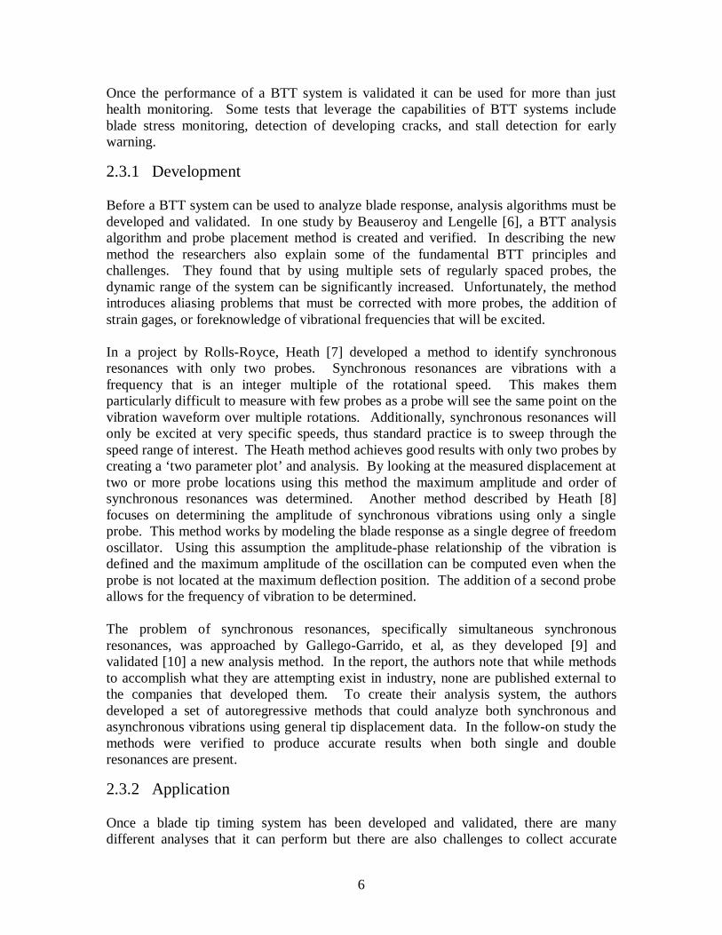
data. Osburn [11] used a commercial two probe tip timing system and applied Heath’s analysis methods. The results were corroborated using a digital photography system and a light pulse timed off of the rotor position. Blade movement indicated resonance was achieved and the method was confirmed using data from the AFRL. Although the Navy Postgraduate School (NPS) rotor did resonate as expected, the deceleration sweep could not be controlled and was too rapid for the probes to collect sufficient data. In a later study also from the NPS, Murphy [12] used an improved system and methods to analyze the vibrations of a NASA rotor. In the testing, large deflections due to surge were observed as well as normal vibration due to exciting the first bending mode. Additionally, the frequency shift due to blade untwist was recorded while sweeping the rotor speed. The results were in excellent agreement with the NASA predications for the rotor, as shown in the Campbell Diagram in Figure 3. The Campbell Diagram is a graph of rotor speed and vibration frequency which shows where the synchronous excitations cross the blade natural frequencies and excessive vibration occurs.

Figure 3. Campbell Diagram for NPS BTT rotor results and NASA predictions. The orange, blue and beige data points

overlay the NASA predition of blade natural frequency (red line). W. P. Murphy, "High-Speed Blade Vibration in a Transonic Compressor," Monterey, 2008. Public Domain

One field that is seeing increasing interest is crack detection. Some systems [13] are able to use only angular position and shaft vibration sensors to detect cracks forming in the disk of a rotating machine. Others use blade tip timing system so that cracks in blades, specifically at the root of a blade, can be detected. These systems [14] look for shifts in the resonance frequencies or deviation from the standard blade deformation when under centrifugal and aerodynamic load. Part of the difficulty with detecting cracks is that the changes to the blade response vary depending on the shape, location, and severity of the crack. Because of this, multiple methods may be necessary to detect a crack in a blade or

8

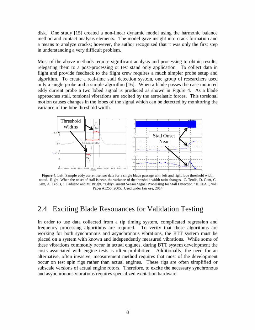
disk. One study [15] created a non-linear dynamic model using the harmonic balance method and contact analysis elements. The model gave insight into crack formation and a means to analyze cracks; however, the author recognized that it was only the first step in understanding a very difficult problem. Most of the above methods require significant analysis and processing to obtain results, relegating them to a post-processing or test stand only application. To collect data in flight and provide feedback to the flight crew requires a much simpler probe setup and algorithm. To create a real-time stall detection system, one group of researchers used only a single probe and a simple algorithm [16]. When a blade passes the case mounted eddy current probe a two lobed signal is produced as shown in Figure 4. As a blade approaches stall, torsional vibrations are excited by the aeroelastic forces. This torsional motion causes changes in the lobes of the signal which can be detected by monitoring the variance of the lobe threshold width.

Figure 4. Left: Sample eddy current sensor data for a single blade passage with left and right lobe threshold width

noted. Right: When the onset of stall is near, the variance of the threshold width ratio changes. C. Teolis, D. Gent, C. Kim, A. Teolis, J. Paduano and M. Bright, "Eddy Current Sensor Signal Processing for Stall Detection," IEEEAC, vol.

Paper #1255, 2005. Used under fair use, 2014

2.4 Exciting Blade Resonances for Validation Testing In order to use data collected from a tip timing system, complicated regression and frequency processing algorithms are required. To verify that these algorithms are working for both synchronous and asynchronous vibrations, the BTT system must be placed on a system with known and independently measured vibrations. While some of these vibrations commonly occur in actual engines, during BTT system development the costs associated with engine tests is often prohibitive. Additionally, the need for an alternative, often invasive, measurement method requires that most of the development occur on test spin rigs rather than actual engines. These rigs are often simplified or subscale versions of actual engine rotors. Therefore, to excite the necessary synchronous and asynchronous vibrations requires specialized excitation hardware.

Threshold Widths

Stall Onset Near

9

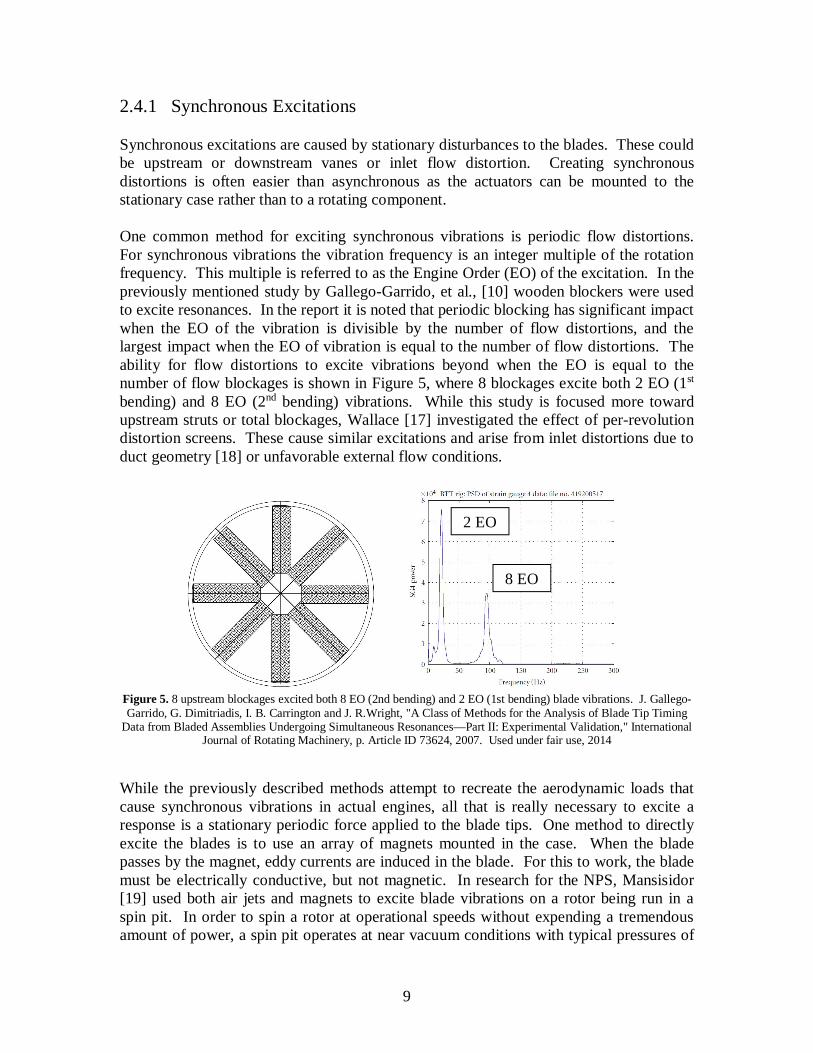
2.4.1 Synchronous Excitations Synchronous excitations are caused by stationary disturbances to the blades. These could be upstream or downstream vanes or inlet flow distortion. Creating synchronous distortions is often easier than asynchronous as the actuators can be mounted to the stationary case rather than to a rotating component. One common method for exciting synchronous vibrations is periodic flow distortions. For synchronous vibrations the vibration frequency is an integer multiple of the rotation frequency. This multiple is referred to as the Engine Order (EO) of the excitation. In the previously mentioned study by Gallego-Garrido, et al., [10] wooden blockers were used to excite resonances. In the report it is noted that periodic blocking has significant impact when the EO of the vibration is divisible by the number of flow distortions, and the largest impact when the EO of vibration is equal to the number of flow distortions. The ability for flow distortions to excite vibrations beyond when the EO is equal to the number of flow blockages is shown in Figure 5, where 8 blockages excite both 2 EO (1st bending) and 8 EO (2nd bending) vibrations. While this study is focused more toward upstream struts or total blockages, Wallace [17] investigated the effect of per-revolution distortion screens. These cause similar excitations and arise from inlet distortions due to duct geometry [18] or unfavorable external flow conditions.

Figure 5. 8 upstream blockages excited both 8 EO (2nd bending) and 2 EO (1st bending) blade vibrations. J. Gallego-Garrido, G. Dimitriadis, I. B. Carrington and J. R.Wright, "A Class of Methods for the Analysis of Blade Tip Timing

Data from Bladed Assemblies Undergoing Simultaneous Resonances—Part II: Experimental Validation," International Journal of Rotating Machinery, p. Article ID 73624, 2007. Used under fair use, 2014

While the previously described methods attempt to recreate the aerodynamic loads that cause synchronous vibrations in actual engines, all that is really necessary to excite a response is a stationary periodic force applied to the blade tips. One method to directly excite the blades is to use an array of magnets mounted in the case. When the blade passes by the magnet, eddy currents are induced in the blade. For this to work, the blade must be electrically conductive, but not magnetic. In research for the NPS, Mansisidor [19] used both air jets and magnets to excite blade vibrations on a rotor being run in a spin pit. In order to spin a rotor at operational speeds without expending a tremendous amount of power, a spin pit operates at near vacuum conditions with typical pressures of

8 EO

2 EO

10

100-200 millitorr. This significantly reduces aerodynamic loads and heating. When air jets are used, the vacuum pumps have difficulty maintaining the desired low air pressure level within the chamber. Magnets, such as the pole reverse pair shown in Figure 6, do not have this shortcoming. The optimum magnet configuration was found to be a pair above the tips of the blades, as well as a pair behind the trailing edge.

Figure 6. Magnet final position for optimal blade synchronous excitation. M. R. Mansisidor, "Resonant Blade Response in Turbine Rotor Spin Tests using a Laser-Light Probe Non-Intrusive Measurement System," Monterey,

2002. Public Domain

2.4.2 Asynchronous Excitations To create an asynchronous excitation, either complex aeroelastic effects are required or a moving simple excitation source is required. To create a test rig to excite either synchronous or asynchronous blade vibrations with the same hardware, Arnold Engineering Development Center (AEDC) [20] used a rotating blockage plate. When kept stationary, the blade response is the same as shown in the previous section. When the blockage plate is spun, however, asynchronous vibrations can be created. As with synchronous excitations, the methods here can be split into aerodynamic and direct blade excitation. The AEDC rig relied on varying aerodynamic loading due to the blockage plate. To directly excite the blades, an actuator must be placed on the blades themselves or mounted to a rotating ring. One actuator that can be mounted directly to the blades is a piezoelectric plate or film. These can be mounted to the blade surface [21] or imbedded into custom blades [22]. Application to the surface of the blades as shown in Figure 7 allows for the use of actual engine hardware with minimal modification.

11

Figure 7. Piezoelectric film actuators mounted to the face of spin rig compressor blades. I. Goltz, H. Böhmer, R. Nollau, J. Belz, B. Grueber and J. Seume, "Piezo-Electric Actuation of Rotor Blades in an Axial Compressor". Used

under fair use, 2014

2.5 Testing Application Detail - Foreign Object Damage One cause of blade failure that is impossible to completely design away or avoid is Foreign Object Damage (FOD). FOD damage can range from the slow abrasion of a blade coating due to sand ingestion to an immediate blade loss and engine failure due to bird ingestion. A BHM system can do little to help in a blade-out scenario; however, for more moderate damage it could alert the crew to repair or replace a blade. In many cases the most dangerous damage is minor notches near the blade root. While these notches do not immediately degrade blade performance, they are excellent crack propagation points. Over many engine cycles cracks will grow from these points in the high stress regions of the blade until the blade structure is compromised and failure occurs. Minor FOD, such as that shown in Figure 8, can be difficult to identify with a visual inspection. A BHM system can record changes in blade dynamics due to either damage or the initial impact ringing.

Figure 8. Small notch in a Garrett F109 fan blade caused by impact with foreign object

12

Even with the scope of FOD narrowed to minor events that can lead to crack growth, simulating FOD on new airfoils or locating actual damaged blades is difficult. Actual damaged blades are often repaired or destroyed, and finding an engine that an owner is willing to deliberately FOD is nearly impossible. For this reason it is useful to look at observational studies of actual FOD before deciding the optimal way to simulate it so that BHM detection methods can be created.

2.5.1 In-Service Engine Observation The military estimated that it spends approximately 400 million dollars annually in HCF related inspection and maintenance [23]. Much of this inspection and repair is necessitated by minor FOD that can lead to crack formation and HCF failure. One study sought to quantify the quantity and extent of FOD on an actual military aircraft blade. Ten randomly selected F404 first stage fan blades were inspected for FOD with the observed impacts shown in Figure 9. The majority of the damage from the impacts are 0.002 inches or less and occur more frequently near the tip of the blade. As the F404 powers the aircraft carrier based F/A-18 Hornet it was determined that much of the minor FOD was due to dislodged anti-skid grit for the carrier flight deck. The larger impacts are far less frequent; however they are spread more evenly along the blade span [24].

Figure 9. Distribution and severity of FOD on 10 randomly selected F404 engine (F18) first stage fan blades. P.

Prevéy, D. Hornbach, J. Cammett and R. Ravindranath, "Damage Tolerance Improvement of Ti-6-4 Fan Blades with Low Plasticity Burnishing," in 6th Joint FAA/DoD/NASA Aging Aircraft Conference, 2002. Used under fair use, 2014

Further analysis of the F/A-18 first stage fan blades found that FOD 0.020 inches deep reduced the blade HCF strength from 100 ksi to 35 ksi [25]. HCF strength reductions this severe could lead to early blade failure; however, if it is detected early enough, the blade could be repaired or replaced during normal maintenance. FOD can also occur in larger extents while not leading to immediate failure. In these cases a BHM system could alert the pilot to land as soon as possible to avoid blade failure. One study identified the cause of one such event after the blade had failed. It was determined that a single rivet was struck by several compressor blades, with the first strike occurring soon after startup. The final strike was to a high pressure compressor

13

(HPC) blade that failed after many engine cycles as shown in Figure 10 [26]. If a BHM system were present the pilot and crew could have been notified of the damage before the HPC blade separation.

Figure 10. Failed HPC blade due to continued operation after impact with a rivet head. G. Morse, "Analysis of Engine

Damage - Engine SN 451-133," Failure Analysis Service Technology, Inc, 2007. Used under fair use, 2014

2.5.2 FOD Simulated for Research With a baseline established by observing FOD on actual blades, most researchers have turned to simulating FOD on representative airfoils and evaluating its impact on test specimen fatigue life. In a study by the AFRL, Ruschau et al [27] used 1 mm glass spheres shot at 305 m/s to damage Ti-6Al-4V test specimens. The impacts left spherical notches on the leading edge of the blade as shown in Figure 11. Off angle impact was found to be more detrimental to fatigue strength than head on, with strength reductions of up to 50%. A similar study by Bache et al [28] found that titanium aluminide blades had lower fatigue endurance levels at room temperature than Ti-6Al-4V blades, but better high temperature performance.

Figure 11. View of head on impact of spherical projectile strike on simulated airfoil. J. J. Ruschau, T. Nicholas and S.

R. Thompson, "Influence of foreign object damage (FOD) on the fatigue life of simulated Ti-6Al-4V airfoils," International Journal of Impact Engineering, vol. 25, pp. 233-250, 2001. Used under fair use, 2014

In another study by the AFRL, Mall et al [29] attempted to identify what components of impact damage are most detrimental to blade fatigue strength. To create more controllable and consistent damage the test used steel indenters pressed into a rectangular

14

specimen rather than projectiles shot at a curved surface. When the observations were coupled with a FE analysis of the deformation, empirical trends for the reduction in fatigue life could be determined based on the depth of macro bands of intense plasticity and residual stresses. Two studies by Xi Chen [30] [31] attempted to bridge the previous two AFRL studies by simulating the impact of a spherical object on a rectangular blade. The study, which used Ti-6Al-4V alloy blades, found that numerical analysis yielded good agreement with physical measurements of stress fields, and that simple dimensionless formulas could be developed that give insight into the fatigue strength reduction. While most studies focus on spherical or cylindrical indentation, Nowell, et al., [32] approached the problem from a worst case for stress concentrations, the V-notch. The paper is a study on the stress concentrations and crack propagations caused by this extreme FOD geometry.

2.6 Summary and Introduction to the Present Research A commercial BTT system requires extensive sensor, algorithm, and signal processing development as well validation testing. However, once completed the system can be used to extend or even in some cases replace intrusive measurement methods such as strain gages. The literature shows great increases in capabilities of BTT systems in recent years that now can function to detect harmful synchronous and asynchronous vibrations that could lead to HCF failure, impact ringing and damage from FOD, and even stall and flutter before full onset. Additionally the means for validating BTT systems have expanded with tip magnets for synchronous excitations and piezoelectric actuators for asynchronous excitation. Even with the recent improvements there is still a need for improved algorithms and more accurate sensors in the field. This thesis will present the fundamental principles and methods of BTT so that a validation method can be devised and tested. In doing so, alternative blade vibration measurement schemes will be developed and vibration analysis tools explored. Improvements to the methods and test hardware will also be discussed as this test program will be continued and expanded to complete the validation of this new commercial BTT system.

15

Chapter 3: Fundamental Blade Tip Timing Methods

3.1 Introduction At its most fundamental level, a blade tip timing system only records the time of arrival of each blade relative to a non-vibrating reference point. To determine deflection, frequency and amplitude requires advanced algorithms and knowledge of the rotor geometry. But before that is even possible, the BTT system must determine when a blade tip arrives and do so consistently. The blade tip deflections in small turbomachines are typically on the order of thousandths of an inch, which when the blade tip is traveling at over a thousand feet per second requires timing resolutions in the micro and nanosecond range. While discussing the fundamental methods of BTT, it is also prudent to highlight the capabilities and limitations of the technology and its competitors. Strain gages, predominantly used before the development of BTT, are probably the closest competitor to BTT systems and are still widely in use today in engine development in spite of their high cost and invasive installation. Strain gages provide direct strain measurement at any position on the blade surface. This strain can then be correlated to stress at any location on the blade using a validated finite element model of the blade. One of the biggest advantages of strain gages is that they record continuous, high response data. There is no need for curve fitting or undersampled data processing as the sensor is constantly measuring the strain at its position. Strain gages have limitations, however. As they are mounted to a single blade they only provide data from that specific blade. Additionally the sensor must be mounted to the surface of the blade which could alter mechanical or aerodynamic response. Strain gages also require slip rings or wireless telemetry systems to transfer the signal from the rotating domain to the stationary data acquisition system. And finally, as the gages are attached to rotating vibrating structures with high speed and possibly heated flow overhead, they are prone to failure during the course of developmental testing and are not useful for in-service health monitoring. BTT systems in contrast can be mounted in the stationary case and therefore are much less expensive to install. Another benefit of being stationary is that one set of BTT probes collects data on all of the blades. The probes are also mechanically robust to case vibration and moderate temperatures, which allow the probes to remain useful longer and open the possibility of in-service health monitoring. And as there are no changes made to the rotating components, the response of the blades is not be impacted by the measurement system. The primary drawbacks to these systems are that measurements are typically limited to the blade tip and measurements can only be made when that tip passes under one of the

16

timing sensors. The probe cannot detect modes that do not cause sufficient (tip amplitude to stress ratio) tip motion, and improper probe spacing or an insufficient number of probes can lead to vibration frequency aliasing. Additionally, if a vibration node is located at the blade tip then a BTT system will not detect the vibration. For these reasons most present-day engine development programs use both strain gages and BTT systems so that the benefits of each can be combined to make a complete measurement system.

3.2 Determining Blade Time of Arrival The structure of the signal returned from the BTT sensor will depend on whether it is a capacitive, eddy current or optical sensor. As the commercial sensors evaluated in this thesis are optical sensors, this overview will consider their signal structure. Even the best raw signal from a BTT probe will not be a sharp square wave or digital signal. Therefore a single arrival time, the TOA, must be selected from the signal curve such as that shown in Figure 12. The methods used include detecting the start of the rise above the noise floor (1), the time at which the signal exceeds a scaled threshold (2), and the time at which the signal falls back to the noise floor (3). Combinations of these values or entire blade passage window based measures can be used as well. Each of these references will choose a different TOA; however, as long as the TOA corresponds to a consistent point on the blade over many revolutions the deflection results will be accurate.

Figure 12. Example TOA points on a blade tip scan. (1) Rise Start, (2) Threshold, (3) Fall End

Optical probes have the capability to have the highest resolution of the tip timing probes; however, they are also the most susceptible to lens fouling or poor signal quality. The very high resolution nature of optical probes, particularly focused optical probes, can be both a positive and a negative. Optical probes can often resolve details such as small scratches or discoloration on the blade tip that can enable the system to recognize specific blades. Conversely, some blade tip conditions can actually cause difficulty for the timing system to choose consistent and accurate TOA points. Some of the problematic blade tip features are shown in Figure 13. These can be caused by unusual tip geometry such as large radius edges or be the buildup of deposits on the blade tip. The noisy baseline can cause rising edge start or falling edge end detection algorithms to be inconsistent. An

17

asymmetric profile could cause poor results out of a blade center finding algorithm. Also, noise or detail near the front face of the signal could cause a simple threshold based method to return inconsistent data. An example of a cause for poor optical signal quality, the uneven buildup of deposits, is shown in Figure 14. This blade will produce a signal that is strong at the pressure and suction edges of the blade but weak in-between. Entirely dark blade tips can reduce the signal to noise ratio sufficiently that some optical probe designs produce inaccurate data.

Figure 13. Example actual blade tip scans that can create noisy data with some TOA algorithms

Figure 14. Image of actual used blade tip from the Virginia Tech Turbomachinery and Propulsion Research Laboratory JT15D. Note the bright pressure and suction edges and dark center of the blade tip

18

Typically the effect of these features on a well-setup system is minor, as these features are usually larger than the change in blade relative position due to vibration. Because of this the feature is often present in the probe signal throughout the blade vibratory motion and therefore does not have an effect on the measurement of the blade relative position. Still, on in-service blades it has been observed that there is no one best method depending on blade tip geometry and condition. For this reason the evaluated system collects a full suite of TOA values so that the post processing software or the operator can select the TOA method that returns the best results. Once the TOA of each blade is accurately determined, the BTT system can convert the values into deflections. An example of how to select the TOA method is provided in Appendix A using data off of the Virginia Tech JT15D.

3.3 Converting Time of Arrival to Blade Deflection As there are no direct measurements of strain or stress with a BTT system, the deflection of the blade tip must be determined from the blade TOA relative to the TOA of a rotating reference point. This reference could be a flat or tooth on the rotor that a sensor can trigger from at once per revolution (OPR) or an average position relative to the TOA of the other blades on the rotor. In a perfect rotor, the blades would be equally spaced, the location of the probes precisely known, the speed of the engine constant (or acceleration known), and the reference for the OPR directly in line with blade 1. These assumptions would lead to the following ideal expected blade arrival time (푡 ) after the OPR:

푡 = 푡 + ⁄

+ ⁄

(1)

This equation can be simplified using angles between components to:

푡 = 푡 + ( ) ⁄( )⁄

+ ( )( )⁄( )⁄

(2)

푡 = 푡 + 푇 + ( ) 푇 (3) where 푡 is the time that the OPR is triggered, 휃 is the angular position of the probe relative to the OPR, B is the blade number (OPR is in line with blade 1, increase with rotation), N is the total number of blades, and 푇 is the time for one complete rotation of the disk. While this analysis would likely prove to be sufficient to identify the blades, it is insufficient for vibration deflection measurements due to the manufacturing tolerances of the rotor and instrumentation placement. These tolerances along with blade untwist due to rotational forces will create a static offset from the ideal TOA as shown in Figure 15. The blade vibration is a dynamic deflection superimposed over this static offset.

19

Figure 15. The ideal blade TOA are used as the reference for the actual blade TOA offset which is used as the

reference for determining blade vibratory deflection

Therefore, the static deflections of the blades and misalignment of the sensors must be considered. To accomplish this, the test rig or engine is typically run at a quiet (low expected vibrations) speed and the 푡 is used to calculate each blade’s deflection. These deflections will be each blade’s static offset (훿 ) as seen by each probe and are found as follows:

훿 = ∆푡 (4)

∆푡 = 푡 − 푡 (5) where 푅 is the radius from the rotation axis of the engine to the blade tip and 푡 is the TOA that the probe records for each blade. With the deflections of each blade recorded by each sensor and averaged over several rotor speeds and many revolutions, the “stack plot” may now be generated as seen in Figure 16. This plot shows the deflection, or more accurately the offset, of each blade as reported by each sensor. The probes should be in near agreement with one another on a specific blade’s displacement; however, each blade’s offset may vary. The variation in blade offset over the entire rotor is due to imperfections in the disk and blades, while the variation in offset for a single blade is due to probe misalignment. Both can be accounted for in equation 6 to remove the manufacturing and placement error. This leaves only the assumption of constant rotor speed during a revolution, which often is an acceptable assumption. To verify, a shaft multi-per-rev (2, 3, 4…N) could be installed and rotor speed could be updated multiple times during a revolution. Leveraging the previous equations, the vibration deflection of each blade (훿) as seen by each probe can be computed by:

훿 = ∆푡 + 훿 + 훿 (6)

20

Figure 16. Stack Plot with simulated data for the average result from 8 probes on a 17 blade rotor

With the quiet or average offset setting the new reference, the deflection away from this reference can be isolated as the blade tip vibratory deflection. In the case of synchronous vibration, a single probe will see the same point on the vibration waveform so that the blade could appear to not be vibrating. In the case of asynchronous vibration there will be a clear distribution of amplitudes around the reference offset. An example of this is shown in Figure 17 where blade 1 is resonating at a non-integer multiple of the rotational speed. If blade 1 were not resonating, its deflection distribution would be similar to that of the other 11 blades.

21

Figure 17. Actual blade deflection distribution data over 500 rotations from a single probe on a 12 blade rotor with blade 1 (bottom) resonating

3.4 Optimizing Timing Probe Placement The placement of BTT probes is critical to determining the correct vibration amplitude and frequency. Incorrect spacing can lead to either no vibration being observed, or incorrect frequency and amplitude. For a single vibration mode the sensors must be placed close enough to ensure that the response is not missed or aliased to a lower frequency as shown in Figure 18. With BTT it is important to know what resonant frequencies and mode shapes are expected so that the probe placement can be optimized. This is particularly important when multiple or crossing modes are possible.

Deflection (mm)

Blad

e N

umbe

r

Blade 12

500 Measurements of Blade 12 Offset

Thickness – Number of Occurrences of Offset Measurement

22

Figure 18. Incorrect probe spacing can lead to no vibration observed for a synchronous event or aliasing if the probes

are too widely spaced. The stars mark the measurement points and the dashed line is the sine curve fit

One method to select probe locations is to characterize blade tip motion as the superposition of sine waves. The response for a single vibration with a period of once per rotation is modeled as a simple sine wave. This frequency of vibration is commonly referred to as an Engine Order (EO) of 1. If a vibration frequency were double the rotational frequency, then it would be a 2 EO oscillation. The blade tip displacement 푑 at any angle 휃 for a 1 EO vibration is given as:

푑 = 푎 + 푎 sin(휃) + 푎 cos(휃) (7) If we look at a single probe location 휃 , the blade displacement observed at this position 푑 is:

푑 = 푎 + 푎 sin 휃 + 푎 cos 휃 (8) The simplest form of this equation normalizes all vibration frequencies to EO:

푑 = 푎 + 푎 sin 퐸푂 휃 + 푎 cos 퐸푂 휃 (9)

23

To fit this equation by conventional means we need at least 3 probes as we have 3 unknown coefficients (푎 ). Four or more probes would be preferred. This method can be extended to multiple concurrent frequencies by adding more terms to the equation and using more probes to collect data: 푑 = 푎 + 푎 sin 퐸푂 휃 + 푎 cos 퐸푂 휃 + 푏 sin 퐸푂 휃 + 푏 cos 퐸푂 휃 (10)

As mentioned above, to fit these vibration models we need more than one probe. To accommodate them we add more equations, which model the displacement at each of the different probe angular locations:

푑 = 푎 + 푎 sin 퐸푂 휃 + 푎 cos 퐸푂 휃 (11) 푑 = 푎 + 푎 sin 퐸푂 휃 + 푎 cos 퐸푂 휃 (12) 푑 = 푎 + 푎 sin 퐸푂 휃 + 푎 cos 퐸푂 휃 (13)

The goal when choosing probe placement locations is to minimize the impact that errors due to noise in the data have on the solution to the set of the equations. As many solution methods use matrices for computation we will convert our system of equations into a matrix equation:

푑푑푑

=1 sin 퐸푂 휃 cos 퐸푂 휃1 sin 퐸푂 휃 cos 퐸푂 휃1 sin 퐸푂 휃 cos 퐸푂 휃

푎푎푎

(14)

The condition number of a matrix gives the ratio of the maximum and minimum singular values of the matrix. Completing the condition number of the matrix in equation 14 will give us a number indicating how sensitive a set of probe locations is to noise. This in turn will give an indication of the uncertainty in our resulting analysis and curve fit. The ideal condition number is 1; however condition numbers up to 6 are likely acceptable [33]. Thus, the condition number for a single given engine order (EO) and three selected probe locations (휃 ) is:

퐶표푛푑푖푡푖표푛 푁푢푚푏푒푟 = 푐표푛푑1 sin 퐸푂 휃 cos 퐸푂 휃1 sin 퐸푂 휃 cos 퐸푂 휃1 sin 퐸푂 휃 cos 퐸푂 휃

(15)

While many BTT analysis methods do not attempt to directly curve fit the data, using this method results in the most independent set of probe locations for the physical vibration which will produce the best results regardless of analysis method.

24

3.5 Predicting Vibration Mode Frequencies Before the probe placement method in section 3.4 can be implemented, the frequencies and EO of interest must be identified. The blade modal frequencies are predicted by finite element analysis and can be validated by laser vibrometry. As part of this project, analysis was completed on a P&WC PT6A-28 first stage rotor that will be used for future BTT validation testing. The disk and blades were purchased used from an overhaul shop in the condition as shown in Figure 19. If the rotor design geometry is not known, as is the case with the PT6 rotor, then the blade must first be 3D laser scanned and 3D modeled to support the FE analysis. The scanned geometry CAD file generated by GKS Laser Design is shown in Figure 20. This geometry, with only minor modification and repair, was exported as a step file and imported into ANSYS Mechanical for FE analysis.

Figure 19. PT6A-28 first stage compressor rotor as received from overhaul shop, Airforce Turbine Service

Figure 20. PT6A-28 hardware scanned and 3D modeled for FE analysis, GKS Laser Design

25

Once a complete 3D model of the blade was imported into ANSYS Workbench, the material properties needed to be determined. The blade material was not known however it was assumed to be titanium TI-6Al-4V or stainless steel 17-4 PH. To confirm several tests were completed. One difference between the materials is that the stainless steel is magnetic while the titanium is not. The PT6 blade was not magnetic. Another difference is the density of the materials. The density of stainless steel 17-4 PH is 7.8 g/cm3 while that of Ti-6Al-4V is 4.43 g/cm3. The density of the PT6 blade was 4.5 g/cm3. Both of the above tests indicated that the blade material is likely titanium, as summarized in Table 1. This assertion is further supported by a Pratt and Whitney Canada blade coating report where the purpose was to evaluate the performance of a blade coating on Ti-6Al-4V blades and one of the test articles was a PT6 first stage compressor blade [34].

Table 1. Material properties of PT6 blade and possible blade materials

Material PT6A-28 Blade Stainless Steel 17-4 PH

Titanium Ti-6Al-4V

Magnetic No Yes No Density 4.5 g/cm3 7.8 g/cm3 4.43 g/cm3

Young’s Modulus ? 197 GPa 114 GPa Poisson Ratio ? 0.272 0.33

With the material properties determined the blade model was meshed using the ANSYS Workbench Mesher. One priority when meshing a part for mechanical analysis is to ensuring that the mesh does not artificially impact the results, that is, to ensure grid independence. The final mesh used in the analysis is shown in Figure 21; however, several coarser meshes and a finer mesh were also generated so that frequency convergence could be confirmed. The monitored parameter was the 3rd mode frequency as it was the highest mode of interest and higher frequency modes require finer meshes to resolve. Figure 22 shows a plot of the calculated 3rd mode frequency for each successive refinement.

26

Figure 21. Final refined PT6A-28 Blade FE mesh

Figure 22. 3rd Mode frequency mesh convergence plot. The finest refinement (100k elements) was selected for the analysis

The modal stationary modal analysis was performed using ANSYS Mechanical and Workbench. Typically the strongest response is due to one of the first three modes; however, depending on the frequency of excitation higher modes may need to be

27

computed. For the PT6 rotor only lower modes will be directly excited and are likely to produce a significant component of the blade vibration. The first two bending modes and first torsional mode for a PT6A-28 first stage compressor blade are shown in Figure 23. When coupled with the rotor speed and the excitation frequency, these modal frequencies will determine the engine orders of interest in the probe positioning method described in the previous section.

Figure 23. The first three mode shapes and frequencies for the PT6A-28 blade from an ANSYS Mechanical modal analysis. Red is motion out of the page, blue is motion into the page, and green is stationary

Before testing can be conducted or excitation designs can be completed, the FE mode frequency results must be experimentally validated. For this testing the modes were validated using a laser vibrometry instrument from Polytec. The same blade that was scanned for the FE model was excited acoustically while being scanned by a laser vibrometry system. The measured mode shapes were in excellent agreement with the predictions, as shown by the experimental results in Figure 24 and tabulated mode frequencies in Table 2. Except for the third mode which has an error of nearly 4%, for all other modes the FE model had errors of less than 1%. These results are considered to be

1st Bending 1966 Hz

2nd Bending 7144 Hz

1st Torsion 5539 Hz

28

in sufficient agreement that the FE model can be extended to predict the effect of rotation on the modal frequencies of the blade, particularly for the first and second modes.

Table 2. FE and experimental vibration mode frequency summary

Mode FE Frequency (Hz) Measured Frequency (Hz)

Model Error (%)

1st 1966 1959 0.36 2nd 5539 5584 -0.81 3rd 7144 6875 3.91 4th 9398 9400 -0.02 5th 11228 11175 0.47

Figure 24. The experimental mode shape results from laser vibrometry scan of the blades. Red is motion out of the page, blue is motion into the page, and green is stationary

3.6 Summary of Vibration Frequency Extraction Methods Even once the probes are properly placed and the TOA data accurately collected, advanced signal processing is still required for spectral analysis of the blade vibration. This is due to the two inherent problems with BTT data: undersampling and non-uniform sample points. The former rules out simple interpolation between the probes to produce satisfactory results. The latter eliminates traditional uniform FFT and spectral analysis methods. To process general timing data, more general methods are required. The method used for extracting vibration frequency and amplitude depends on whether the vibration is synchronous with the rotor rotation or asynchronous. If synchronous, the BTT probes are used to capture blade resonance as the rotor is accelerated through the resonance exciting speed. Then the blade response is modeled as a single degree of freedom oscillator. Using this assumption the amplitude-phase relationship of the vibration is defined and the maximum amplitude of the oscillation can be computed. When using two or more probes with the single degree of freedom method, the vibration frequency can also be determined.

29

For asynchronous vibration more vibration waveform data is available as the position of the deflection pattern on the rotor changes every rotation. Many methods involve fitting a sine wave model to the data. Doing so fills in the missing data between the non-uniform sampling points, while not blindly influencing the data as a simple interpolation would. As this method is fitting sine curves to the data, it is apparent why the sine wave model probe placement method is useful. Many systems, including the Prime Photonics BTT system, use similar or combinations of these methods for their proprietary analysis methods.

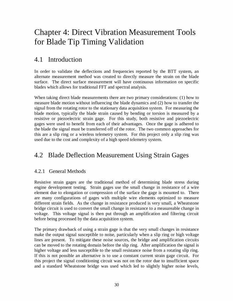
30

Chapter 4: Direct Vibration Measurement Tools for Blade Tip Timing Validation

4.1 Introduction In order to validate the deflections and frequencies reported by the BTT system, an alternate measurement method was created to directly measure the strain on the blade surface. The direct surface measurement will have continuous information on specific blades which allows for traditional FFT and spectral analysis. When taking direct blade measurements there are two primary considerations: (1) how to measure blade motion without influencing the blade dynamics and (2) how to transfer the signal from the rotating rotor to the stationary data acquisition system. For measuring the blade motion, typically the blade strain caused by bending or torsion is measured by a resistive or piezoelectric strain gage. For this study, both resistive and piezoelectric gages were used to benefit from each of their advantages. Once the gage is adhered to the blade the signal must be transferred off of the rotor. The two common approaches for this are a slip ring or a wireless telemetry system. For this project only a slip ring was used due to the cost and complexity of a high speed telemetry system.

4.2 Blade Deflection Measurement Using Strain Gages

4.2.1 General Methods Resistive strain gages are the traditional method of determining blade stress during engine development testing. Strain gages use the small change in resistance of a wire element due to elongation or compression of the surface the gage is mounted to. There are many configurations of gages with multiple wire elements optimized to measure different strain fields. As the change in resistance produced is very small, a Wheatstone bridge circuit is used to convert the small change in resistance to a measureable change in voltage. This voltage signal is then put through an amplification and filtering circuit before being processed by the data acquisition system. The primary drawback of using a strain gage is that the very small changes in resistance make the output signal susceptible to noise, particularly when a slip ring or high voltage lines are present. To mitigate these noise sources, the bridge and amplification circuits can be moved to the rotating domain before the slip ring. After amplification the signal is higher voltage and less susceptible to the small resistance noise from a rotating slip ring. If this is not possible an alternative is to use a constant current strain gage circuit. For this project the signal conditioning circuit was not on the rotor due to insufficient space and a standard Wheatstone bridge was used which led to slightly higher noise levels,

31

most of which was higher frequency and was filtered out. To ensure that the noise was not having a detrimental impact on the results a piezoelectric sensor was added to also measure blade strain. The position where a strain gage is adhered to the blade surface is also important, particularly with complex modern blade designs. When a blade is vibrating, regions of high stress and strain can be confined to small portions of the blade, as shown in Figure 25 of the FE model-predicted strain field for the PT6 blade at the first bending mode. Placing the strain gage near the leading edge or the tip would result in a much lower signal from the gage.

Figure 25. Strain field from FE analysis of a PT6A-28 blade at first bending mode from the ANSYS Mechanical modal analysis

4.2.2 Application to Current Research For this research, a strain gage system was assembled from components procured from Omega Engineering. The gages used had a grid length of 3mm and a nominal resistance of 350 ohms. They were standard linear 1-axis gages, temperature matched to aluminum. The gage was wired through the slip ring to a quarter Wheatstone bridge completion circuit. The circuit also included a balancing potentiometer to help tune its high precision and temperature stable internal resistors. The output from the completion circuit was connected to a strain gage amplification and filtering circuit. The amplifier had adjustable gain and the low pass filter was set at its maximum of 2,000Hz. The output from the amplifier and filtering circuit was connected to an Agilent oscilloscope for observation and recording of data. An overall schematic of the system is shown in Figure 26.

Low strain location

High strain location

32

Figure 26. The test configuration for the strain gage on blade vibration measurements

The Omega DMD-465WB Bridge signal conditioner consisted of an AC power supply, a bridge excitation supply, an instrumentation amplifier and a 2 kHz Bessel filter. The power for the unit was standard 115V AC. The excitation power supply is up to 15V and includes voltage sensing leads to compensate for long wires to the Wheatstone bridge. The differential instrumentation amplifier has an adjustable gain from 40 to 250 and a common mode rejection of 90 to 100 dB depending on the selected gain. The Bessel filter range is adjustable with the addition of external capacitors. However for this project it was left at its maximum DC to -3 dB frequency of 2,000 Hz. A summary schematic from the product manual [35] is shown in Figure 27.

Figure 27. Omega DMD-465WB strain gage amplification and filtering circuit. Omega Engineering Inc., "DMD-

465WB Bridgesensor AC Powered Signal Conditioner," 1999. Used under fair use, 2014

33

4.3 Blade Vibration Measurement Using Piezoelectric Sensors

4.3.1 General Methods Piezoelectric sensors and actuators are part of a large family of devices that deform when a voltage is applied to their electrodes or produce a voltage when their structure is deformed. This makes them ideal for both causing a structure to deform or vibrate and for sensing strain on a structure. One common configuration is a plate with electrodes on the top and bottom surfaces. When the plate is stretched or compressed it produces a voltage; therefore, when the plate is mounted to the surface of a structure it makes an excellent strain gage. Additionally, as the output voltage is induced by the strain in the material the sensor is passive; no excitation power supply is required. The output voltage is also very large, which means that the piezoelectric sensor does not require amplification. One drawback, however, is that the charge in the plate bleeds off quickly so the sensor is not effective at measuring static strain. As with the resistive strain gage a piezoelectric gage must be placed in a region of high strain for the mode being measured, otherwise the response will be low or non-existent.

4.3.2 Application to Current Research There are many sizes of piezoelectric plate material available with further customization available by cutting the plates. For this work 7x8x0.2mm plates were used to attain high signal strength while minimizing the impact on the blade mechanical structure. For this research the piezoelectric strain sensor setup was much less complex than the resistive strain gage system as shown in Figure 28. This was because no amplification or filtering was required to collect acceptable data. As with the strain gage, the piezoelectric plate was directly wired to the slip ring. The only special consideration when mounting the sensor was to ensure that the ground side of the plate was facing the blade as the blade face was grounded. Once through the slip ring the signal lines went directly to the oscilloscope through twisted pair wire for observation and recording. Due to the high voltage amplitude of the signal no additional conditioning was found to be necessary.

Figure 28. The piezoelectric sensor system required only the sensor connected to the oscilloscope through the slip ring

34

4.4 Signal Transfer Using Slip Rings In both of the previously described strain sensor systems, a slip ring was at the heart of the system. A slip ring is a device that makes an electrical connection between stationary and rotating wires. This is usually accomplished by wire brushes or liquid conductor connections. Careful alignment and low vibration are necessary to protect the slip ring at high speeds; however, contact resistance will still vary between the brush and ring leading to signal noise while rotating. Slip rings are usually specified by number of conductors, maximum speed, and the electrical capabilities of the conductors. Figure 29 shows the schematic of a four conductor wire brush slip ring. One major drawback to the design shown in the schematic is that there is no shielding and only minimal separation between the brushes and rings. This can lead to crosstalk and noise between the conductors, particularly if there are power and data conductors in the same slip ring. Insulated conductor slip rings are available; however, if possible power and data should be split into separate slip rings.

Figure 29. Schematic of a four conductor wire brush slip ring

The Moog EC3848 slip ring used in this research was donated by Moog Components Group. The slip ring has 10 one amp 100 volt conductors and can operate uncooled at up to 10,000 RPM. It is a compact face mount slip ring measuring only 1.1 inches long and 0.75 inches wide. Additionally, it uses precious metal fiber brush contacts to minimize

35

noise at high speed for data or power circuits [36]. The assembled slip ring is shown in Figure 30.

Figure 30. Moog EC3848 10,000 RPM 10 circuit high speed slip ring

36

Chapter 5: Validation I Methods and Testing – Blade and Probe Static Offset

5.1 Introduction The foundation of a BTT vibration detection system is an accurate static offset measurement. Without this baseline, vibratory deflection amplitude cannot be accurately determined as vibration is motion relative to the static offset. Therefore in developing the sensors and algorithms for a BTT system a logical first step is to verify static offset performance. In an actual turbomachine engine and BTT system, there are two sources of uncertainty as to when a non-deflected blade should arrive at a timing sensor. The first is the manufacturing tolerance of the rotor and blades. Every blade and blade dovetail are slightly twisted, bent, or offset from the nominal design location resulting in the blade tips not being precisely equally spaced. These deviations are small, often in the low or sub millimeter range and should not impact the performance of the rotor. However, for a timing system with deflection resolution well below one millimeter, these offsets must be accounted for to accurately calculate blade deflection. The second contribution to TOA offset is the actual positions of the timing probes. Once again the minute errors in probe circumferential spacing and radial angle result in even a non-deflected blade arriving at each probe at a slightly different time relative to the OPR sensor. This actual rotor blade position must be determined before any deflection analysis can observe vibration or static deflection. In addition to determining the static offset of each blade and probe, the BTT system must also be able to index each blade relative to the OPR sensor. The static offset, deflection, and frequency analysis all need data collected over multiple rotations for a single blade. If on one rotation a blade were to be missed and no indexing scheme was present, TOAs for different blades would be inadvertently combined as if from the same blade. Also if the BTT system were used as a health monitoring system then a blade that experienced a FOD strike or high vibration must be able to be identified.

5.2 Machined Blade Offset Rotors The goal of the first developed validation method is to create a rotor with known static blade offsets so that the reported offsets from a BTT system can be evaluated. For this test method to provide accurate results, the rotors must be designed so that they have minimal blade vibration and rotating deflection. Due to the high resolution of modern BTT systems, the rotors must be machined and measured precisely as the smallest imperfections and offsets will be detected by the system.

37

5.2.1 Design and TOA Measurement To evaluate the static offset performance of the BTT system two “blisk” rotors were machined using a CNC mill. The rotors were designed to fit in a four inch diameter spin rig powered by a router motor. The spin rig is capable of speeds from 8,000 to 25,000 RPM and has an optical OPR sensor. Twelve sensor mounts are equally spaced around the metal pipe shroud. Figure 31 shows the spin rig with a rotor installed. For the offset testing the rotors were spun at the minimum speed of 8,000 RPM to minimize deflection and vibration.

Figure 31. High speed router spin rig that was used for the static offset testing

The first rotor was designed with uniformly spaced blades, while the second had the blade positions offset slightly in a “sine wave” pattern around the circumference. Both rotors were made of aluminum and had short blades to minimize tip deflection and vibration. With the uniform rotor we would expect to see offsets of nearly zero (within the manufacturing accuracy of the CNC mill). For the sine wave rotor we would expect to see the offset pattern that was built into the rotor. By defining a specific blade spacing pattern the blade TOA offsets were known so that the BTT sensors and algorithms could be validated. To simplify manufacture and improve manufacturing accuracy, both blisks employed simplified blade geometry. The rotor and blade construction was considered sufficiently similar to conventional practice for the experiment to be valid related to actual operational bladed rotors. This rotor blade design is referred to as a ‘paddlewheel’ due to its blades having a flat rectangular shape closely resembling that of a water paddlewheel, as shown in Figure 32 for a 24 blade rotor.

Sensor Mounts

OPR Sensor

Rotor

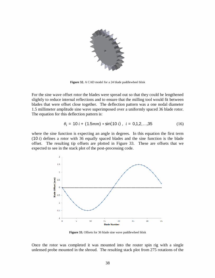
38

Figure 32. A CAD model for a 24 blade paddlewheel blisk

For the sine wave offset rotor the blades were spread out so that they could be lengthened slightly to reduce internal reflections and to ensure that the milling tool would fit between blades that were offset close together. The deflection pattern was a one nodal diameter 1.5 millimeter amplitude sine wave superimposed over a uniformly spaced 36 blade rotor. The equation for this deflection pattern is:

휃 = 10 푖 + (1.5푚푚) ∗ sin(10 푖) , 푖 = 0,1,2, … ,35 (16) where the sine function is expecting an angle in degrees. In this equation the first term (10 푖) defines a rotor with 36 equally spaced blades and the sine function is the blade offset. The resulting tip offsets are plotted in Figure 33. These are offsets that we expected to see in the stack plot of the post-processing code.

Figure 33. Offsets for 36 blade sine wave paddlewheel blisk

Once the rotor was completed it was mounted into the router spin rig with a single unlensed probe mounted in the shroud. The resulting stack plot from 275 rotations of the

39

rotor is shown in Figure 34. This result, while shifted in phase from Figure 33 due to a different blade defined as blade 1, is qualitatively in excellent agreement for amplitude and shape. In setting the static offsets we are primarily interested in the average offset reported by the BTT system; however, the stack plot also provides insight into vibration and blade instability. While there is a small tail of outliers to the right of each blade location, most of the reported offsets are tightly clustered around the average position. This indicates that the vibration amplitude is very low for all of the blades, as was desired when designing this rotor. The blade offsets are defined from the mean deviation (or deflection) from where evenly spaced blades would be. The average blade offsets for the sine wave rotor are shown in Figure 35.

Figure 34. Blade deflection distribution plot from 275 rotations of the sine wave rotor using an unlensed probe

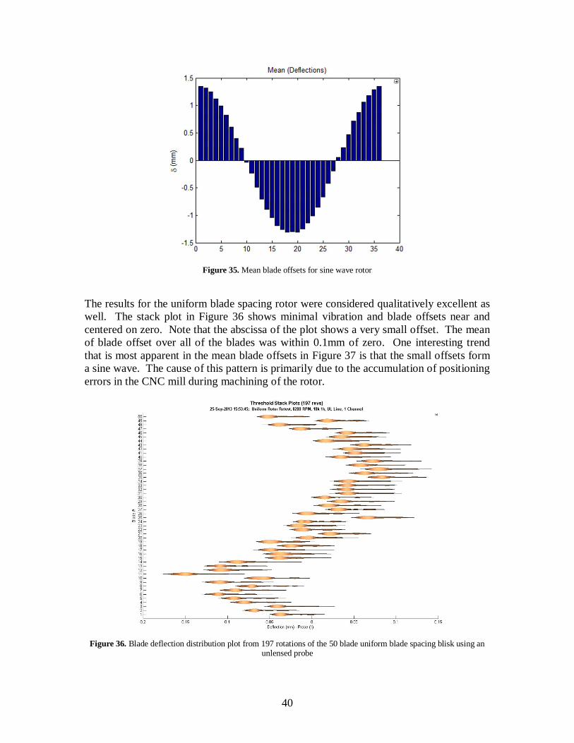
40

Figure 35. Mean blade offsets for sine wave rotor

The results for the uniform blade spacing rotor were considered qualitatively excellent as well. The stack plot in Figure 36 shows minimal vibration and blade offsets near and centered on zero. Note that the abscissa of the plot shows a very small offset. The mean of blade offset over all of the blades was within 0.1mm of zero. One interesting trend that is most apparent in the mean blade offsets in Figure 37 is that the small offsets form a sine wave. The cause of this pattern is primarily due to the accumulation of positioning errors in the CNC mill during machining of the rotor.

Figure 36. Blade deflection distribution plot from 197 rotations of the 50 blade uniform blade spacing blisk using an

unlensed probe

41

Figure 37. Mean blade offsets for 50 blade uniform spacing blisk with unlensed probe

5.2.2 Measuring Blade Offset for Tip Timing Result Validation While from the previous figures it is clear that the general trends and amplitudes expected in the blade offsets are observed in the BTT data, an alternate measurement method was needed to quantitatively confirm this. As these rotors are simply straight extruded two dimensional shapes, a document scanner was used to create a high resolution image of the face of each of the rotors. The images were then imported into CAD software where the leading edge, trailing edge, and midpoint radii were marked. The blade spacing starting from the marked blade 1 was then defined at the angle between the midpoints of each blade as shown for the sine wave offset rotor in Figure 38. This process was repeated for the uniform spacing rotor as well.

Figure 38. Static deflections for 36 blade sine wave paddlewheel blisk.

42

Before the scanned offsets were compared with the BTT results the uncertainty in the offset calculations was quantified. The uncertainty for the angle of the leading and trailing edge radii was set by bounding the possible angles of TOA trigger due to manufacturing defects on the surfaces and pixel resolution of the image. The midpoint radius was defined from the leading and trailing edge causing the uncertainty to combine as a sum of squares. The uncertainty in edge radii angle was found to be 0.14 degrees which results in a midpoint offset uncertainty of approximately ±0.1 millimeters for a 4 inch rotor. The testing was completed using the 8,000 RPM spin rig and a single unlensed probe. The measured BTT offset results were within 0.13 millimeter of the scanned rotor results, with only a few blades falling outside the 0.1 millimeter scan uncertainty range as shown in Figure 39. For the uniform rotor, a similar sinusoidal trend is visible in both the scan and the BTT offset data as shown in Figure 40, indicating that at least part of the unexpected curve was machined into the rotor. For this rotor there are more BTT points that lie outside the uncertainty bounds. This is not unexpected as the uniform rotor has more and smaller blades. On these smaller blades the manufacturing defects impact a larger portion of the blade tip, resulting in a higher blade to blade TOA trigger point variation. The uncertainty bands for both data sets were set by analysis of the sine wave rotor blade tips and scan. As the static deflection measurement is the baseline for dynamic measurements it is imperative that the results were accurate and repeatable. These tests show excellent agreement between the measurements made by the rotor scan method and the tip timing system.

Figure 39. Blade offset for the sine wave rotor from optical scanning and BTT using an unlensed probe

43

Figure 40. Blade offset for the uniform rotor from optical scanning and BTT using an unlensed probe

5.3 Blade Indexing Validation As there is no physical sensor mounted to a blade for BTT measurements, an important step is identifying and indexing each blade. Rather than choosing the first blade observed, a blade is selected and located relative to the OPR sensor. If a blade TOA is assigned to the incorrect blade any curve fitting or interpolation algorithms will produce erroneous results. The validation method developed to test blade indexing is to create a blade offset pattern with a sharp discontinuity between the last blade and blade 1 as shown in Figure 41. If the BTT system correctly identifies blade 1 and has the correct spacing between the other blades then it is correctly indexing the blades.

44

Figure 41. By using an offset pattern with a sharp discontinuity, the blade 1 identification by a BTT system can be

verified

To evaluate the blade indexing on the commercial BTT system, blade offset measurements were collected from the flat black plastic rotor shown in Figure 42. The rotor was made from ABS plastic to reduce machining time. The rotor had a ramp (saw tooth) pattern machined into the blade offset so that a sharp discontinuity would occur at an easily identifiable blade (blade 1). Using the unlensed sensors, accurate data was collected off of the flat black rotor. After making minor corrections to the blade indexing algorithm, the system consistently and accurately selected the correct blade 1 as shown in Figure 43.

Figure 42. Saw tooth plastic rotor for blade 1 identification testing

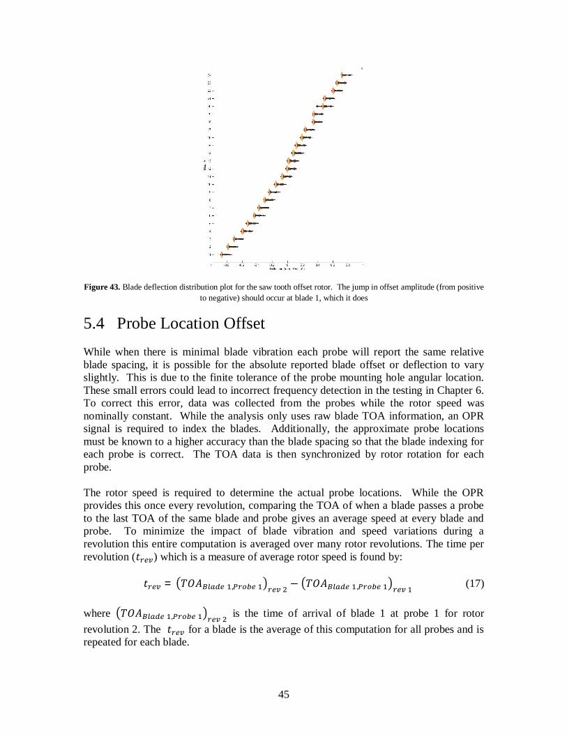
45

Figure 43. Blade deflection distribution plot for the saw tooth offset rotor. The jump in offset amplitude (from positive to negative) should occur at blade 1, which it does

5.4 Probe Location Offset While when there is minimal blade vibration each probe will report the same relative blade spacing, it is possible for the absolute reported blade offset or deflection to vary slightly. This is due to the finite tolerance of the probe mounting hole angular location. These small errors could lead to incorrect frequency detection in the testing in Chapter 6. To correct this error, data was collected from the probes while the rotor speed was nominally constant. While the analysis only uses raw blade TOA information, an OPR signal is required to index the blades. Additionally, the approximate probe locations must be known to a higher accuracy than the blade spacing so that the blade indexing for each probe is correct. The TOA data is then synchronized by rotor rotation for each probe. The rotor speed is required to determine the actual probe locations. While the OPR provides this once every revolution, comparing the TOA of when a blade passes a probe to the last TOA of the same blade and probe gives an average speed at every blade and probe. To minimize the impact of blade vibration and speed variations during a revolution this entire computation is averaged over many rotor revolutions. The time per revolution (푡 ) which is a measure of average rotor speed is found by:

푡 = 푇푂퐴 , − 푇푂퐴 , (17)

where 푇푂퐴 , is the time of arrival of blade 1 at probe 1 for rotor revolution 2. The 푡 for a blade is the average of this computation for all probes and is repeated for each blade.

46

As this computation does not use the OPR beyond blade indexing, the location of the first probe is assumed to be the nominal design location. This assumption does not impact the results because the relative spacing between probes is what is critical to frequency calculations. To determine the location of the second probe the TOA difference between probes 1 and 2 is normalized by 푡 to determine the fraction of an entire rotation that lies between the probes. As we know there are 360 degrees in a full rotation and the first probe nominal location is taken to be its true location (휃 ), the second probe location (휃 ) is:

휃 = 휃 + 360 ∗ , , (18)

This computation is then repeated for each successive probe using the previous probe average as the reference. Once the location of each probe is computed from a single blade revolution, this process is repeated for all blades over many rotations. The actual probe location is approximated as the average of these values. Table 3 shows the results of applying this method to a Prime Photonics BTT system with four probes. While the correction is often small, it can be significant for closely spaced probes.

Table 3. Correction of probe locations using TOA data over 100 rotor revolutions

Probe # Nominal Location (deg)

Average Measured (deg)

Standard Deviation (deg)

Probe 1 30 30 (reference) N/A Probe 2 50 49.965 0.184032 Probe 3 88.966 88.92662 0.276765 Probe 4 91.034 90.84639 0.028971

47

Chapter 6: Validation II Methods - Exciting Dynamic Deflections

6.1 Introduction When classifying the vibration of turbomachinery blades and blisks, one usually divides them into synchronous (or integral) and asynchronous (non-integral). The cause of synchronous vibrations in an actual engine is often circumferentially constant upstream or downstream distortions that excite blade resonances at a specific set of speeds. Asynchronous vibrations are instead caused by complex aeromechanical interactions such as flutter or stall. Exciting either in a test environment is challenging, as creating full scale models of the parts is often too costly or too complex to allow for the mounting of the required measurement equipment. This is particularly true for BTT development, where we are not interested in reproducing a specific vibration problem but rather testing whether the BTT sensors can detect a general blade vibration response. As with in an actual engine the methods for exciting synchronous and asynchronous vibrations in a test rotor will be different. Synchronous excitation requires a forcing function that is fixed to the casing so that the excitation frequency is a function of the rotation speed. Asynchronous excitation, however, needs a forcing function that is independent of the rotation speed, which lends itself to a blade-mounted solution. Finally, it is important that the two systems are independent so that the effects can be superimposed to test the BTT system’s ability to distinguish mixed vibration responses.

6.2 Exciting Synchronous Vibrations When discussing synchronous excitations, the Campbell diagram is a commonly used tool to help visualize the relation between rotor speed, excitation frequency and blade modal frequency. This diagram is a plot of the vibration frequency versus the rotor speed. The first step in creating one of these plots is to draw the synchronous excitation lines. These lines, also known as the EO lines, are straight lines that extend out from the origin as shown in Figure 44. These lines predict which blade vibration frequencies various EO excitations (integer multiples of the rotation speed) will excite. At this stage the plot offers limited insight into the vibration characteristics of the blade as typical synchronous distortions will not excite large blade response unless the excitation frequency coincides with one of the blade resonant frequencies. The range of the Campbell diagram is bounded by the rotor operational speeds and the maximum number of excitations.

48

Figure 44. The EO lines show what frequencies will be excited for various EO excitations with rotor speed. For a rotor

operational speed of 0 to 20,000 RPM and 1 to 15 EO excitations

To complete the Campbell diagram the blade resonant frequencies while experiencing rotating stress must be determined. Typically a static FE modal analysis is validated using a clamped blade ping test and then the FE model is used to extend the modal analysis to rotating conditions. A FE model was used to predict the rotating blade modes of the PT6 rotor. In many cases the frequency shift due to rotating stiffening is not large; in the case of the PT6 blade the FE model was used to estimate that the first mode shifts from 1,966 Hz to 2,066 Hz going from zero to 20,000 RPM. The data from the rotating FE modal analysis was added to complete the Campbell plot as shown by the solid lines in Figure 45. The dashed horizontal lines are the non-rotating blade natural frequencies. When the natural frequency curve crosses one of the EO excitation lines there is the potential for synchronous vibrations if the proper excitation or distortion pattern is present. A synchronous vibration test is not only an opportunity to validate a BTT system or FE modal analysis. To excite synchronous vibrations, a rotor speed sweep is executed rather than attempting to sit on the resonance speed. This is because only a specific speed will excite resonance in a blade, and this speed will vary blade to blade due to manufacturing and material variability. Therefore a synchronous sweep test is also an excellent opportunity to evaluate blade manufacturing repeatability, blade interface damping and blisk mistuning.

49

Figure 45. Complete Campbell diagram of PT6 blade first three modes with example 5EO crossing at 2,125 Hz and 25,500 RPM

In an actual engine these EO excitations can be caused by vanes or struts near the rotor. No matter how the engine is designed the EO excitations will exist and EO lines may even cross modes; however, the crossings must be traversed quickly or avoided altogether for safe operation. In a test environment distortion excitations from screens or struts can still be used. Magnets are an alternative where stronger excitations are necessary or in a vacuum spin pit where air density is low. A magnet pair mounted in the shroud generates a magnetic field in the vicinity of the blade tip. As the blade passes through this field, eddy currents are generated in the blade by the varying magnetic field strength. These induced currents and the presence of the magnetic field create a force that deflects the blade. As the blade passes through an evenly spaced set of magnet pairs a synchronous forcing function is created. As the rotor is swept through its operational range the blade vibration amplitude will increase when the excitation order of the magnet set excites a bending mode. An important feature to note of this excitation method is that although magnets are used, the blade does not have to be magnetic. It does need to be conductive though, so this method will be ineffective with composite or non-metallic tip blades. Another design consideration is that the thermal conductivity of the blade material must be high enough to dissipate the eddy current tip heating. In low thermal conductivity materials such as titanium this can even lead to the blade tips melting.

50

6.3 Exciting Asynchronous Vibrations The asynchronous excitation method selected for this research was piezoelectric actuators. When a voltage differential is applied to a piezoelectric plate, the length of the plate extends or retracts depending on the polarity of the signal relative to the plate poles. A single plate with electrodes on the front and back faces would not bend in such a way to create a blade deflection. Therefore two plates are needed with a single structural element for strength between them as shown in Figure 46. When this center element is a thin metal plate, the resulting device is a piezoelectric bimorph actuator.

Figure 46. Due to the opposite orientation of the piezoelectric plates one plate contracts while the other expands when

a voltage is applied to the bimorph actuator, causing the device to bend

Actuators constructed in this manner are both accurate and high response. When a constant voltage is applied the actuator will deflect and hold that position. When an AC or variable frequency is applied the actuator will bend at that frequency – rotational speed has no impact on excitation frequency. Deflection is highest at the first and second bending resonances and limited by the frequency response of the piezoelectric driver and actuator system. Torsional modes are not excited as the expansion and contraction of the piezoelectric plates creates pure bending. Unlike piezoelectric stack actuators that typically require 1 kV for maximum excitation, many plate actuators require only 100V making them ideal for use with standard voltage slip ring systems. The actuators can also be used for synchronous excitation if the OPR (or multiple-per-revolution) sensor is used as input into the piezoelectric driver.

51

Chapter 7: Validation II Testing - Dynamic Deflection

7.1 Introduction In order to validate tip timing based dynamic deflection and frequency algorithms a known tip vibration must be produced. There are two ways in which this could be done: actively and passively. For the passive method an alternate measurement device is mounted on the blades such as a strain gage or piezoelectric sensor. When the rotor is spun the natural vibrations of the rig are recorded by both the BTT system and the strain gage system. The vibrations may be augmented by a tip magnet system or upstream distortion. To produce non-integral vibrations, however, this system can become very complex requiring rotating distortion screens or high response speed air jets. For the active method some form of actuator is placed on the blade itself and used to directly excite the metal rather than indirectly exciting with airflow. This method does require power as well as data to be transferred into the rotating domain; however, it has the major advantage of easily producing non-integral vibrations. For this reason the dynamic vibration validation method developed in this research uses a blade with active vibration excitation.

7.2 Active Vibration Excitation Rotor Spin Rig

7.2.1 Spin Rig and Drive Design and Construction To implement active vibration excitation on a rotor blade would require significant changes to any of the existing research spin rigs. So that none of the rigs would have to be taken offline a second rig was designed and built with a slip ring for data and power incorporated into the design. This new rig had several changes to make the system more flexible and put less wear on the slip ring. Both excessive speed and vibration can cause the slip ring to fail prematurely; therefore, the rig was designed to operate from very slow speeds up to 3,600 RPM. This speed is well below the slip ring maximum speed of 10,000 RPM, and the speed can be ramped up slowly so that unbalance vibrations or misalignment could be corrected before damage occurred.

The new spin rig used an existing DC variable speed electric motor and speed controller. The maximum output of the motor is 1.5 HP and 1,800 RPM. In order to reduce shaft vibration and increase the maximum speed the rotor shaft is belt driven off of the electric motor with a 2:1 pulley speed ratio. Two high speed SKF bearings were selected so that future tests could further increase rotor speed if needed. A CAD model of the new test rig is shown in Figure 47.

52

Figure 47. CAD Model of new HCF Rig

The new design incorporates a sliding shroud system that makes accessing and removing the rotor simple. The shroud is 6 inches in diameter to accommodate more complex and larger rotor designs and there are now more sensor mount points. Two photographs of the new spin rig in an early stage of construction are shown in Figure 48.

Figure 48. Construction of new HCF Rig

The rotor design was kept simple to reduce development time and sources of error. The design is very similar to the sine wave paddlewheel rotor used in the static deflection validation testing. However, now the fixed aluminum blades are replaced by

53

piezoelectric bending actuators such as those shown in Figure 49. The rotor design utilizing these blades is shown in Figure 50. Not all of the blades must be piezoelectric actuator blades; however; most can be dummy aluminum blades with vibration data analyzed off of only the piezoelectric blades. The other blades are required for balance and to provide a complete set of blades for BTT blade indexing lock.

Figure 49. Acquired Piezoelectric Bending (Bimorph) Actuator

Figure 50. Active Rotor Design (12 piezoelectric bimorph blades shown)

Once mounted in a cantilever configuration, the bimorph actuators are capable of deflections of up to 0.5-1 mm. The actuators can also be used in a passive configuration where, rather than inputting a control voltage, the voltage generated by the actuators is measured. This voltage will give deflection data similar to a strain gage.

To power and control the actuators the piezoelectric power supply was connected to a function generator. The function generator creates the desired waveform and frequency and the power supply amplifies the signal to the desired strength. The piezoelectric power supply as well as one of the test actuators is shown in Figure 51. Strain gages can still be mounted to the blades to measure the actual deflection (in the presence of motor and rotating vibration).

54

Figure 51. Piezoelectric power supply and mounted bimorph actuator

The piezoelectric bimorph actuator selected for this research was the STEMiNC Piezo 40 x 10 x 0.5 mm parallel bimorph actuator. This actuator has a rated maximum tip deflection of 2 mm. It is designed for tip deflection applications and has a maximum input voltage of 100V peak to peak. The piezoelectric plates are made of SM311 piezoelectric material. During trials and testing the actuator was driven by a 5V to 110V Physik Instrumente E-660 Piezo Driver.

In order to transfer both data and power to the rotor a high speed miniature slip ring has been acquired. The slip ring is a Moog Components Group EC3848 High Speed slip ring with 10 circuits. It has a maximum voltage rating of 100V and current rating of 1A. Thanks to its precision ball bearings and precious metal contacts it can operate at up to 10,000 RPM without cooling. With its small size the slip ring will not significantly obstruct airflow if a realistic rotor geometry were tested in the spin rig. A CAD model of the slip ring mounted is shown in Figure 52.

Figure 52. Model of slip ring mounted in new spin rig

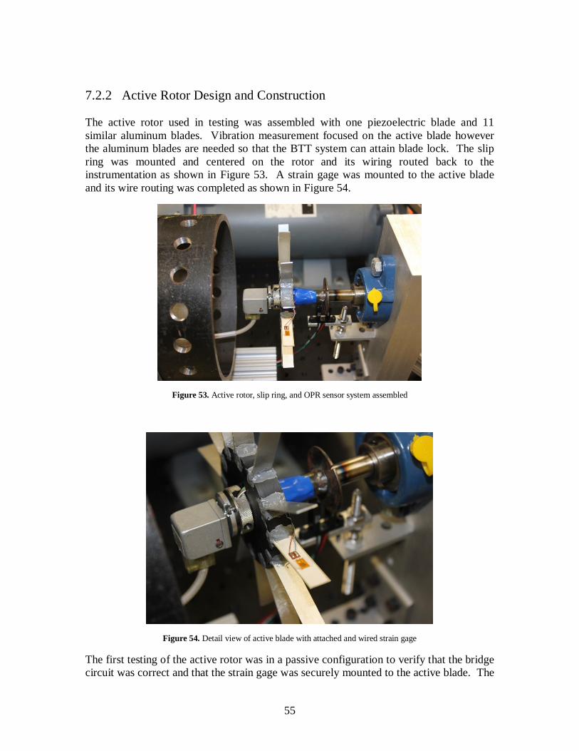
55

7.2.2 Active Rotor Design and Construction The active rotor used in testing was assembled with one piezoelectric blade and 11 similar aluminum blades. Vibration measurement focused on the active blade however the aluminum blades are needed so that the BTT system can attain blade lock. The slip ring was mounted and centered on the rotor and its wiring routed back to the instrumentation as shown in Figure 53. A strain gage was mounted to the active blade and its wire routing was completed as shown in Figure 54.

Figure 53. Active rotor, slip ring, and OPR sensor system assembled

Figure 54. Detail view of active blade with attached and wired strain gage

The first testing of the active rotor was in a passive configuration to verify that the bridge circuit was correct and that the strain gage was securely mounted to the active blade. The

56

same piezoelectric principles that cause the active blade to bend when a voltage is applied make it an excellent dynamic strain gage. As an initial test, data such as that shown in Figure 55 were collected to ensure the sensors and conditioning systems were working as expected.

Figure 55. Voltage created by passive piezoelectric blade, recorded while spinning

Before the active rotor could be used in the frequency validation testing the mechanical response of the blades was determined. This was important so that the frequencies observed by the strain gages and BTT system could be identified and reasonable excitation frequencies selected.

The active blade is composed of three materials: SM311 piezoelectric material, brass, and adhesive. As the brass and adhesive are thin and located at the center of the active blade where bending stresses are lowest, the blade was modeled as a solid sheet of piezoelectric material in ANSYS Mechanical. The results for the first three computed modes are shown in Figure 56. In order to maximize tip deflection amplitude, the testing excitation frequencies will be around the first bending mode predicted frequency of 171 Hz.

57

Figure 56. The (a) first bending, (b) second bending, and (c) first torsion modes for the piezoelectric active blade

The aluminum blades were modeled as cantilever flat plate rectangular solids in ANSYS Mechanical. While these blades will not be directly excited, forcing from the motor vibration and active blade resonance will cause them to vibrate. The first three modes were computed with the results shown in Figure 57. As these frequencies are well above the planned excitation frequency of the active blade, induced vibration should be low as it is forced vibration rather than resonance.

Figure 57. The (a) first bending, (b) second bending, and (c) first torsion modes for the aluminum plate blades

As the first bending mode of the aluminum blade is well above the active blade excitation frequency range, the results of the FE model were not validated. The active blade modes were validated using a coarse harmonic excitation sweep and fine tuning the frequency near the expected point of first bending resonance. The harmonic sweep in Figure 58 shows that the first bending mode was approximately where expected at 175 Hz however the second bending mode is somewhat spread out, likely due to the strain gages mounted

(a) 450 Hz (b) 2810 Hz (c) 3383 Hz

(a) 171 Hz (b) 1067 Hz (c) 1314 Hz

58

on the blade. Fine tuning of the excitation frequency determined that near 1030 Hz resulted in the highest second bending response. When the active blade excitation frequency was manually tuned to the first bending resonance of 175 Hz the tip deflection, shown in Figure 59, was nearly 2 mm. This amplitude is easily detectable by a BTT system and can be reduced to determine the minimum detectable deflection for a BTT system.

Figure 58. A harmonic sweep of the active blade showing a clear first bending mode and a spread second bending

mode

Figure 59. Active blade at first bending resonance, 175 Hz

First Bending –

175 Hz

Second Bending –

950-1050 Hz

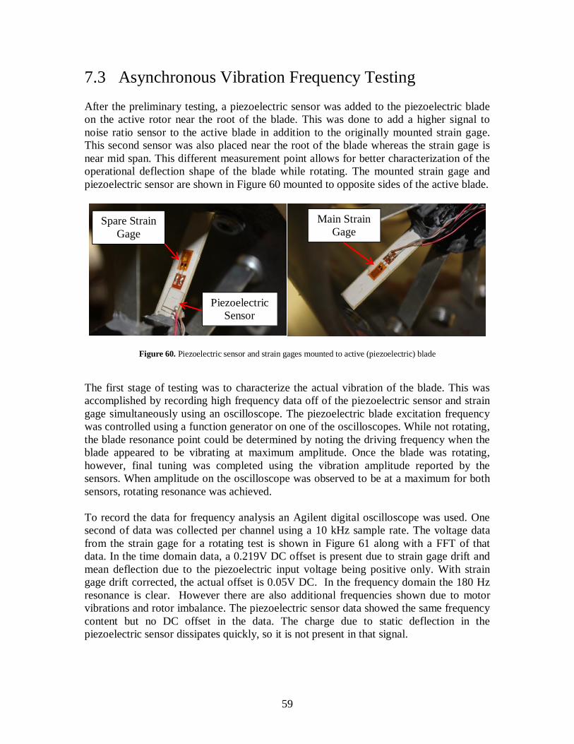
59

7.3 Asynchronous Vibration Frequency Testing

After the preliminary testing, a piezoelectric sensor was added to the piezoelectric blade on the active rotor near the root of the blade. This was done to add a higher signal to noise ratio sensor to the active blade in addition to the originally mounted strain gage. This second sensor was also placed near the root of the blade whereas the strain gage is near mid span. This different measurement point allows for better characterization of the operational deflection shape of the blade while rotating. The mounted strain gage and piezoelectric sensor are shown in Figure 60 mounted to opposite sides of the active blade.

Figure 60. Piezoelectric sensor and strain gages mounted to active (piezoelectric) blade

The first stage of testing was to characterize the actual vibration of the blade. This was accomplished by recording high frequency data off of the piezoelectric sensor and strain gage simultaneously using an oscilloscope. The piezoelectric blade excitation frequency was controlled using a function generator on one of the oscilloscopes. While not rotating, the blade resonance point could be determined by noting the driving frequency when the blade appeared to be vibrating at maximum amplitude. Once the blade was rotating, however, final tuning was completed using the vibration amplitude reported by the sensors. When amplitude on the oscilloscope was observed to be at a maximum for both sensors, rotating resonance was achieved. To record the data for frequency analysis an Agilent digital oscilloscope was used. One second of data was collected per channel using a 10 kHz sample rate. The voltage data from the strain gage for a rotating test is shown in Figure 61 along with a FFT of that data. In the time domain data, a 0.219V DC offset is present due to strain gage drift and mean deflection due to the piezoelectric input voltage being positive only. With strain gage drift corrected, the actual offset is 0.05V DC. In the frequency domain the 180 Hz resonance is clear. However there are also additional frequencies shown due to motor vibrations and rotor imbalance. The piezoelectric sensor data showed the same frequency content but no DC offset in the data. The charge due to static deflection in the piezoelectric sensor dissipates quickly, so it is not present in that signal.

Piezoelectric Sensor

Spare Strain Gage

Main Strain Gage

60

Figure 61. Time and frequency domain strain gage signal for active blade rotating at 2200RPM while resonating at 180 Hz

Testing was also completed with the piezoelectric actuator at maximum static deflection. With the rotor stationary the maximum input voltage of 100V was observed to cause a tip deflection of approximately 0.025 inches. The BTT data in Figure 62 indicates an average blade 1 offset of 0.75 mm for no deflection and 0.25 mm for maximum deflection. This indicates a static deflection of approximately 0.5 mm or 0.02 inches, which is in good agreement with the stationary test.

Figure 62. Switching the piezoelectric voltage from 0V (Left) to 100V (Right), the BTT system reported a static offset change of 0.5 mm. The left scale in both figures is in millimeters

With the blade vibration frequency determined by the strain gage and piezoelectric sensors, focused optical spot sensors were mounted to the shroud and blade tip timing data was collected with the blade resonating at 180 Hz. The tip timing sensors were placed at 30°, 50°, 90°, and 270°. The data was processed using an analysis code provided with the system to determine deflections and vibration frequency. The two strongest frequency components from the piezoelectric sensor (120Hz and 180Hz) were detected as the two strongest components in the BTT spectral analysis as shown in Figure 63. While this analysis data is output directly from the BTT software, Appendix B gives a method for curve fitting the raw BTT data to determine vibration frequency and amplitude.

180 Hz Active Blade

Resonance 120 Hz Motor

Vibration

Blade 1 0V: -0.75 mm

Blade 1 100V: -0.25 mm

61

Figure 63. Active rotor sweep from 1500 RPM to 2500 RPM and resonating at 180 Hz, FFT from piezoelectric sensor compared with spectral analysis of blade tip timing data. Note that the tip timing magnitude is in dB while the strain

gage is in raw voltage

One of the main benefits of blade tip timing is that all of the blades are measured. With the active instrumented blade confirming that the tip timing system is working, the vibratory response of the other blades can be inspected. The 120Hz vibration is caused by a strong electrical hum from the DC motor. This hum is due to the way that the motor controller converts the supplied 60 Hz AC into the variable voltage DC that the motor requires. This frequency does not change with speed. Due to this frequency driving the entire rotor it is expected that all blades show strong response at this frequency as shown in Figure 64. The 180Hz frequency is due to the active blade resonance therefore the active blade should have the highest deflection magnitude. Due to the strength of the resonance all blades are driven at 180Hz which is also shown in Figure 64.

62

Figure 64. The 120Hz motor vibration causes a strong vibration on all blades, while the 180Hz piezoelectric vibration

is highest on the active blade

With maximum active blade tip amplitude easily detectable by the tip timing system, non-resonant frequencies were also attempted to see if their reduced amplitude was still detected. This is important as for this validation method to be useful a wide range of frequencies needs to be producible so that the BTT system can be validated under many conditions. The frequencies tested were 110 Hz, 150 Hz, 200 Hz, and no excitation. The spectral analysis from the BTT system for these excitations is shown in Figure 65 through Figure 68. In the three cases where a piezoelectric excitation was present the excitation frequency was clearly detected along with the 120 Hz motor frequency. In the case of no excitation only the 120 Hz motor frequency was detected across all of the blades. When the active blade was resonating at maximum amplitude the strength of the vibration forced the other blades to vibrate at 180 Hz as well. With the active blade off resonance at 110 Hz the vibration amplitude is significantly lower. This reduction in amplitude results in the aluminum blades no longer responding at the active blade driving frequency as shown in Figure 69. Only the active blade is reported to vibrate at 110 Hz and all blades continue to be driven by the 120 Hz motor vibration.

63

Figure 65. The active blade excited at 110 Hz

Figure 66. The active blade excited at 150 Hz

Figure 67. The active blade excited at 200 Hz

110 Hz Piezoelectric

Excitation

120 Hz Motor

Vibration

150 Hz Piezoelectric

Excitation 120 Hz Motor

Vibration

200 Hz Piezoelectric

Excitation

120 Hz Motor

Vibration

64

Figure 68. All blades with no active blade excitation

Figure 69. Detail View of all blade response with 110 Hz active blade excitation

The wide BTT probe spacing in the testing thus far (minimum 20 degrees) reduces the detectable frequency range of the system. In order to detect second bending at 1036 Hz, one of the focused optical spot probes was replaced with an unlensed optical probe that was equivalent to several probes in just a two degree span. This resulted in measurements at 9°, 10°, 11°, 30°, 90°, and 270°. With this new probe configuration the second bending mode at 1036 Hz was captured along with the motor vibration of 120 Hz. The spectral analysis of the BTT signal is shown in Figure 70.

120 Hz Motor

Vibration

120 Hz Motor

Vibration

110 Hz Piezoelectric

Excitation

65

Figure 70. Active blade with 1036 Hz excitation resulting in second bending resonance

7.4 Methods to Increase Spin Rig Capabilities In order to extend test capabilities to include actual aircraft rotors, initial planning has been completed for creating a spin rig with a PT6A-28 rotor. One major concern exposed by the modal analysis in sections 3.5 and 6.2 is whether the rotor can be spun at sufficiently high speeds for synchronous excitation. To determine the approximate power requirements of the PT6 first stage rotor, a simple mean line analysis of the geometry was completed. The velocity triangles in Figure 71 were created from the blade CAD model. Airflow was assumed to follow the blade metal angles through the entire speed range. Inlet flow was set as axial as in the spin rig there will be no inlet or outlet guide vanes.

Figure 71. PT6 blade velocity triangles at 10,000 RPM – β1 and β2 were approximated from the CAD model of the

blade

With the relative and absolute blade angles approximated, the rotor stage power (푃 ) is found by [37]:

1036 Hz Piezoelectric

Excitation 120 Hz Motor

Vibration

66

푃 = 푚̇ ∗ 푈 ∗ 푈 − 퐶 ∗ (tan(훼 ) + tan(훽 )) (19)

where 푚̇ is the mass flow rate, 푈 is the blade speed at the mean radius, 퐶 is the axial velocity, 훼 is the incoming absolute flow angle and 훽 is the outgoing relative flow angle. For the first stage of the PT6 rotor the estimated power at 10,000 RPM and atmospheric conditions is over 30 HP. The maximum design speed of the PT6 compressor is approximately 35,000-40,000 RPM. Even 10,000 RPM would require a large electric motor and heavy duty drive system as well as a special enclosure due to the high airflow. In a vacuum spin chamber, however, where pressures are typically on the order of 200 millitorr, the power required would be under 0.1 HP to maintain speed. If speeds in excess of 5,000 RPM are desired for the PT6 test rig, the use of a vacuum spin chamber will be considered.

67

Chapter 8: Discussion of Results

8.1 Introduction This section summarizes the major results of this thesis while following the order of the body sections of the report. As the goal of this thesis research was to develop methods to evaluate the performance of a novel blade tip timing system. First, the fundamental BTT methods and validation measurement techniques are discussed. Following is a summary of the first evaluation test method, the blade and probe offset validation. Finally, the results from the first stage of the second evaluation test method, dynamic vibration testing, are presented.

8.2 Methods of Blade Vibration Measurements While the basic theory behind BTT vibration measurements appears simple, attaining the required TOA accuracy and processing the highly undersampled signal is difficult and unreliable without independent verification. The first stage is to determine the blade TOA. Multiple TOA metrics must be computed and recorded to ensure accurate and continuous blade data is collected. Some blade tip geometries or conditions can cause poor TOA results. The methods discussed in Section 3.2 include rise start, fall end, and a threshold on the leading face of the sensor signal. While the method of Section 3.3 to determine blade deflection from the raw TOA and OPR data is straightforward, it illustrated three difficulties in attaining good BTT data. The first is that probe placement is critical for synchronous excitations as the vibration does not rotate relative to the casing. A method is presented in Section 3.4 to ensure the vibration is characterized. The other two are that both blade offset and probe position must be accurately measured to provide a baseline for any vibration calculations. Methods to accomplish this and testing to validate the results are presented in Chapter 5. Once the deflection of each blade is accurately determined at each sensor, frequency algorithms can be applied. While basic methods are discussed at the end of Chapter 3 some of these were already implemented by Prime Photonics, therefore they were not a focus of this thesis. Understanding their similarity to sine curve fitting was important to determining the best validation methods. Strain gages and piezoelectric sensors directly mounted to the blade surface give continuous data on the strain at that point. As discussed in Chapter 4, this can be combined with a validated FE model to estimate the deflection of the tip of the blade. The continuous signal from these devices allows for the use of traditional FFT and frequency analysis methods. A slip ring or wireless telemetry system transfers this continuous signal from the rotating domain to the stationary data acquisition system. A slip ring was used for this thesis due to its much lower cost and complexity.

68

8.3 Static Offset Testing The static offset and probe location sets the baseline for dynamic deflection measurement. For this reason these parameters are the first items to be tested when evaluating a BTT system. To test the static offset and blade indexing features of the system three custom rotors were manufactured. The ramp offset rotor in Section 5.3 allowed for the blade indexing to be validated after minor corrections to the system. Two other rotors were designed, one with minimal blade offset and one with a sine wave pattern to the blade offsets. These rotors were imaged and measured to create an alternate measurement of the blade offset. The BTT blade offsets were within 0.13 mm of the scanned offsets with 0.1 mm uncertainty prescribed to the scanned results, assumed due to manufacturing defects and scan resolution. For computing the frequency of blade vibrations, accurate knowledge of the BTT probe relative positions is essential. A method measuring the probe locations using only the TOA of indexed blades is presented in Section 5.4. While probe angle corrections were all less than 0.2 degrees, some of the probes were spaced only 2 degrees apart. This 10% correction could lead to a substantial improvement in the vibration frequency calculation.

8.4 Dynamic Deflection Testing The overarching goal in this work was to develop test methods that would evaluate the vibration detection capabilities of a BTT system. To validate a BTT system synchronous and asynchronous vibration must be created on a rotating blade. As discussed in Chapter 6, to create synchronous vibrations the excitation source is typically fixed to the engine case and its frequency is an integer multiple of the rotor speed. For an asynchronous vibration the excitation is typically fixed to the blade and its frequency is not an integer multiple of the rotation speed. For this testing, a special active rotor spin rig was designed and built. The spin rig as described in Chapter 7 used a piezoelectric blade to create tip deflections of various amplitudes and frequencies. The blade has a first bending resonance near 180 Hz where tip deflection can be up to 2 mm. A static non-rotating deflection of nearly 0.5 mm was observed by the BTT system as a 0.5 mm blade offset. Frequency analysis of BTT data with the piezoelectric blade at resonance identified deflection at 120 and 180 Hz. Data from the strain gage and piezoelectric sensor confirmed resonance at 180 Hz and a significant vibration component at 120 Hz from the motor. This test was repeated at the second bending resonance, 1036 Hz, with the same successful frequency identification. Non-resonant forced excitation of the active blade was also detected by the BTT system at 110 Hz, 150 Hz, and 200 Hz. Sections 3.5, 6.2 and 7.4 investigated the feasibility of, and began initial planning, for implementing a test rig with realistic rotor geometry. This rotor would use magnets for synchronous excitation and piezoelectric actuators for asynchronous excitation. The

69

rotor would be a PT6A-28 first stage compressor rotor. A Campbell diagram was generated from a FE model of the blade that indicated non-rotating natural frequencies of 1966, 5539, and 7144 Hz. A laser vibrometry scan of the blade validated the frequencies to within 4% and supported the mode shape predictions. The predicted Campbell diagram indicated that high rotational speeds of 10,000 RPM or greater would be helpful in exciting the first three modes of the blades with less than 16 EO excitation. A turbomachinery stage power analysis found that the power required to spin the rotor at only 10,000 RPM would already be in excess of 30 HP in atmospheric pressure air. At a standard vacuum spin chamber pressure of 200 millitorr the power required would be well under 1 HP to maintain rotor speed.

70

Chapter 9: Conclusions and Recommendations

9.1 Conclusions This research developed two innovative validation methods that were used to experimentally evaluate the performance of a novel blade tip timing system. The research focused on creating known blade tip offsets and tip vibrations so that the results from a BTT system could be validated. The topic of result validation is important to the BTT field as the results between many commercial systems still are not consistent. For the first test method custom rotors were created with specified blade tip offsets. These tip offset measurements are the baseline for determining dynamic deflection making their accuracy critical to system performance. Optical scanning was able to determine tip location to an uncertainty of 0.1 mm. The BTT system agreed with the scanned results to within 0.13 mm. In order to correctly assign measurements and responses to physical blades, blade identification and indexing algorithms must be validated. A rotor with a large step machined into the blade offsets was used to validate that the BTT system was selecting the correct blade 1. A method to correct the probe relative locations using only the TOA of indexed blades found probe offsets of less than 0.2 degrees; however, as some of the probes were spaced only 2 degrees apart this correction could still have a significant impact on vibration frequency computations. With the baseline offsets accurately determined, the next stage is to measure any deviation from the baseline. This is the true purpose of the BTT system, as without this capability validated the system cannot be trusted to detect harmful HCF vibrations or damage due to FOD. The active vibration rotor was able to create measureable deflection over a range of frequencies centered on the first bending mode of the blade. The validation rig was able to produce measurable tip deflection at 110 Hz, 150 Hz, the 180 Hz first bending resonance, 200 Hz, and the 1036 Hz second bending resonance. The BTT system performed well in this testing, correctly identifying the active blade excitation frequencies as well as the 120 Hz frequency from the drive motor. It also identified a static tip deflection of 0.5 mm that was created by the active blade while vibrating. Future validation testing will require more representative blade geometry and synchronous vibration testing. Special probe placement algorithms were explored that use sine curve fitting to optimize the probe placement so that synchronous vibrations can be detected. Knowing how the blade will vibrate at operation before testing is critical as well. In preparation for future work using actual engine hardware, ANSYS Mechanical was used to predict the first three modes of a PT6A-28 first stage rotor blade at 1,966, 5,539, and 7,144 Hz. These frequencies were validated to within 4% using scanning laser vibrometry. The simulation was repeated at speed to produce a Campbell Diagram to highlight synchronous excitation crossings which are the point where harmful blade resonances could occur.

71

9.2 Recommendations The results of this research will guide the continued development on the BTT system. Some of the main limitations of this research are due to the active rotor design and test environment. Leveraging the experience of this test a new test system should be built to provide more realistic blade geometry and more controlled blade vibrations. The current active rotor used thin aluminum and piezoelectric blades in atmospheric air. This environment led to vibrations beyond the desired resonance. Furthermore the system was limited to run at slow speeds due to stress on the rotor and mechanical vibrations. Additionally, the blades were thin flat plates and thus did not respond with similar mode shapes or natural frequencies as does an actual aircraft compressor blade. While actual engine hardware is not difficult to acquire, operating a compressor rotor in atmospheric air requires very high driving power due to the air movement. These shortcomings could be alleviated by operating in a vacuum with a well-balanced drive and compressor rotor. The vacuum significantly reduces the aerodynamic load on the rotor, which one case the estimated power dropped from over 30 HP to well under 1 HP. Balancing of the complete rotor and arbor and a high quality drive will reduce mechanical vibration and allow for higher rotational speeds. And in a vacuum, the rotor blade geometry has minimal impact on power load therefore actual engine hardware can be used to obtain realistic blade mode shapes and natural frequencies.

72

Bibliography [1] B. Stange, "ISA Standards for Turbine Engine Test Cell Instrumentation," ISA,

Wyndham Hotel, Cleveland, 2012. [2] A. J. Sanders, K. K. Hassan and D. C. Rabe, "Experimental and Numerical Study of

Stall Flutter in a Transonic Low-Aspect Ratio Fan Blisk," Journal of Turbomachinery, vol. 126, pp. 166-174, January 2004.

[3] C. R. Hedges, "Computational Fluid Dynamic Model of Steam Ingestion into a Transonic Compressor," Monterey, 2009.

[4] C. Hah, "Flow Instabilities and Non-Synchronous Vibration in a Compressor," in 8th ISAIF, Lyon, 2007.

[5] H. Doi, "Fluid/Structure Coupled Aeroelastic Computations for Transonic Flows in Turbomachinery," 2002.

[6] P. Beauseroy and R. Lengelle, "Nonintrusive Turbomachine Blade Vibration Measurement System," Mechanical Systems and Signal Processing, vol. 21, p. 1717–1738, 2007.

[7] S. Heath, "A New Technique for Identifying Synchronous Resonances Using Tip-Timing," Journal of Engineering for Gas Turbines and Power, vol. 122, pp. 219-225, April 2000.

[8] S. Heath and M. Imregun, "An improved single-parameter tip-timing method for turbomachinery blade vibration measurements using optical laser probes," International Journal of Mechanical Sciences, vol. 38, no. 10, p. 1047–1058, 1996.

[9] J. Gallego-Garrido, G. Dimitriadis and J. R.Wright, "A Class of Methods for the Analysis of Blade Tip Timing Data from Bladed Assemblies Undergoing Simultaneous Resonances—Part I: Theoretical Development," International Journal of Rotating Machinery, p. Article ID 27247, 2007.

[10] J. Gallego-Garrido, G. Dimitriadis, I. B. Carrington and J. R.Wright, "A Class ofMethods for the Analysis of Blade Tip Timing Data from Bladed Assemblies Undergoing Simultaneous Resonances—Part II: Experimental Validation," International Journal of Rotating Machinery, p. Article ID 73624, 2007.

[11] N. Osburn, "Implementation of a Two-Probe Tip-Timing Technique to Determine Compressor Blade Vibrations," Monterey, 2000.

[12] W. P. Murphy, "High-Speed Blade Vibration in a Transonic Compressor," Monterey, 2008.

[13] E. Sonnichsen, "Real-time Detection of Developing Cracks in Jet Engine Rotors," in IEEE Conference, 2000.

[14] M. Zielinski and G. Ziller, "Noncontact Crack Detection on Compressor Rotor Blades to Prevent Further Damage after HCF-Failure".

[15] V. Kharyton, "Faults Detection in Blades of an Aviation Engine in Operation," 2009. [16] C. Teolis, D. Gent, C. Kim, A. Teolis, J. Paduano and M. Bright, "Eddy Current

Sensor Signal Processing for Stall Detection," IEEEAC, vol. Paper #1255, 2005.

73

[17] R. M. Wallace, "Modal Response of a Transonic Fan Blade to Periodic Inlet Pressure Distortion," Blacksburg, 2003.

[18] A. M. Ferrar, "Measurements of Flow in Boundary Layer Ingesting Serpentine Inlets," Blacksburg, 2011.

[19] M. R. Mansisidor, "Resonant Blade Response in Turbine Rotor Spin Tests using a Laser-Light Probe Non-Intrusive Measurement System," Monterey, 2002.

[20] T. Hayes, B. Hayes, T. Tibbals, S. Arnold and J. Davenport, "Spin Rig for NSMS Probe Development and Strain Gage Correlation," in 58th International Instrumentation Symposium, 3rd Tip Timing Workshop, San Diego, 2012.

[21] I. Goltz, H. Böhmer, R. Nollau, J. Belz, B. Grueber and J. Seume, "Piezo-Electric Actuation of Rotor Blades in an Axial Compressor".

[22] G. Maahs, "Design of an Active Compressor Blade for Aeroelastic Studies," 1999. [23] Propulsion Directorate, AFRL/WPAFB, "High Cycle Fatigue (HCF) Program 1999,"

2000. [24] P. Prevéy, D. Hornbach, J. Cammett and R. Ravindranath, "Damage Tolerance

Improvement of Ti-6-4 Fan Blades with Low Plasticity Burnishing," in 6th Joint FAA/DoD/NASA Aging Aircraft Conference, 2002.

[25] Lambda Technologies, "LPB Application Note - Improved Ti-6Al-4V Fan Blade FOD Tolerance".

[26] G. Morse, "Analysis of Engine Damage - Engine SN 451-133," Failure Analysis Service Technology, Inc, 2007.

[27] J. J. Ruschau, T. Nicholas and S. R. Thompson, "Influence of foreign object damage (FOD) on the fatigue life of simulated Ti-6Al-4V airfoils," International Journal of Impact Engineering, vol. 25, pp. 233-250, 2001.

[28] M. Bache, C. Bradshaw and W. Voice, "Characterisation of foreign object damage and fatigue strength in titanium based aerofoil alloys," Materials Science and Engineering, vol. A354, pp. 199-206, 2003.

[29] S. Mall, J. L. Hamrick and T. Nicholas, "High Cycle Fatigue Behavior of Ti-6Al-4V with Simulated Foriegn Object Damage," Mechanics of Materials, vol. 33, pp. 679-692, 2001.

[30] X. Chen, "Foreign Object Damage and Fatigue Cracking," Cambridge, 2001. [31] X. Chen, "Foreign object damage on the leading edge of a thin blade," Mechanics of

Materials, vol. 37, pp. 447-457, 2005. [32] D. Nowell, D. Dini and P. Duo, "Stress analysis of V-notches with and without

cracks, with application to foreign object damage," Journal of Strain Analysis, vol. 38, no. 5, pp. 429-441, 2003.

[33] P. Russhard, "Blade Tip Timing – Frequently asked Questions," in Proceedings of the 58th International Instrumentation Symposium, San Diego, 2012.

[34] W. McNally, "Erosion-Resistant Coating for Titanium," 1973. [35] Omega Engineering Inc., "DMD-465WB Bridgesensor AC Powered Signal

Conditioner," 1999. [36] Moog Components Group, "High Speed Slip Ring Capsules - EC3848".

74

[37] P. Hill and C. Peterson, Mechanics and Thermodynamics of Propulsion (2nd Edition), Upper Saddle River: Prentice Hall, 1991.

75

Appendix A: Selecting the Time of Arrival Method The TOA triggering methods of a BTT system must be flexible so that the highest resolution data can be collected from a given rotor. One actual engine that testing was conducted on is the Pratt and Whitney JT15D at the Virginia Tech Turbomachinery and Propulsion Research Lab. The fan blades of this engine have a dark deposit buildup down the center of the blade with bright edges, as shown in Figure 14. With newer focused light probes the signal was improved substantially from that shown in Figure 13; however, the selection of the TOA method is still an essential step. The TOA method is selected by computing the timing resolution for each TOA method over thousands of rotor rotations. The lowest timing resolution TOA method is then used in the post-test analysis, although all timing points are still collected by the system. Timing resolution can be multiplied by the blade tip speed to determine the deflection resolution. Deflection resolution is typically used in industry when discussing the performance of a BTT system. To measure the timing resolution on a rotor, two probes are placed closely together so that they “see” the blade tip at approximately the same time. The TOA of each blade by each sensor is then collected for several thousand revolutions. The timing resolution is then taken as the variance of the difference between the times of arrival of a blade as reported by each probe. This value is computed for every blade over all of the revolutions, and the average is taken as the timing resolution of the system. By computing this value using two closely spaced probes and the same blade rather than an external reference, the effects of rotor speed variation and vibration are removed except for the short period of time it takes the blade to traverse the distance between probe one and probe two. For this analysis, 4 threshold limits were set each on the rising edges and the falling edges of the raw BTT sensor signal. In Figure 72 is shown a near ideal blade reflectivity profile from the JT15D fan test. Here all threshold points are in a region of very steep rise or fall (rise time is approximately four microseconds with a blade tip speed of 350 m/s). With steep and clean rising and falling edges, a fairly symmetric peak, and a flat and low-noise floor, all of the TOA methods are likely to return good results for this blade. This blade was identified as blade 23 for this test.

76

Figure 72. Great optical blade reflectivity profile on blade 23 from JT15D testing

For the blade identified as blade 3 during this test, the profile was not as ideal. As shown in Figure 73, a large leading edge peak caused one of the falling threshold points to land in a horizontal and noisy region of the falling edge. We would expect this blade to give poor timing resolution for that falling threshold point.

Figure 73. Poor falling edge optical reflectivity profile on blade 3 from JT15D testing

While qualitatively the best TOA methods can be determined by analyzing the reflectivity profiles, during testing the timing resolution computation is used. Table 4

Rising Threshold

Falling Threshold

1 2 3

4 1

2 3 4

Rising Threshold

Falling Threshold

1 2 3

4 1

2 3 4

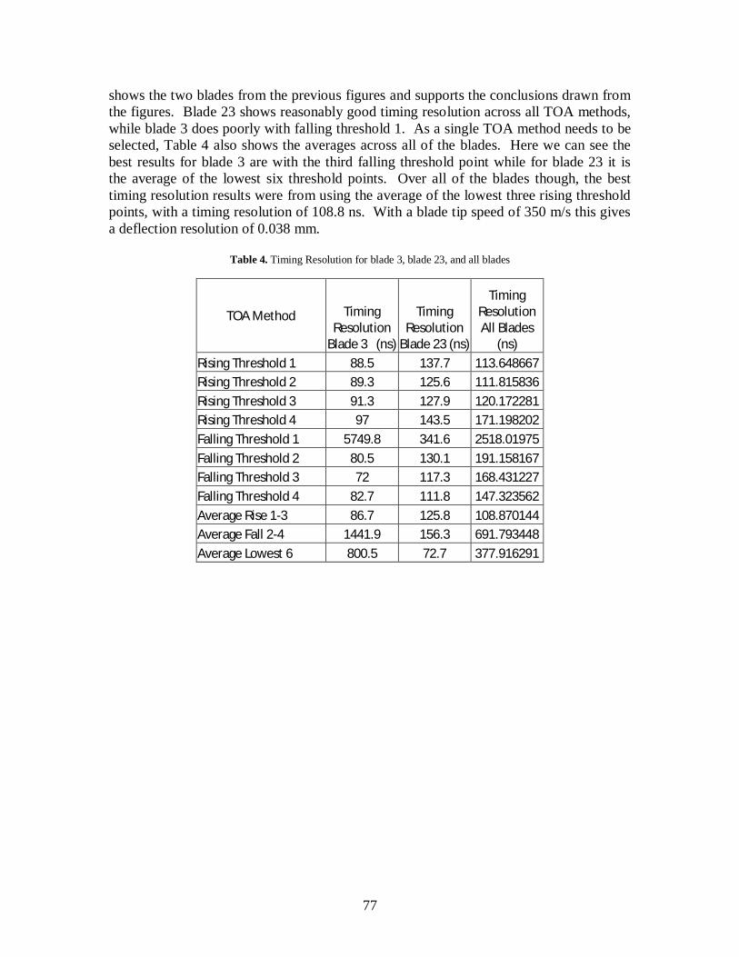
77

shows the two blades from the previous figures and supports the conclusions drawn from the figures. Blade 23 shows reasonably good timing resolution across all TOA methods, while blade 3 does poorly with falling threshold 1. As a single TOA method needs to be selected, Table 4 also shows the averages across all of the blades. Here we can see the best results for blade 3 are with the third falling threshold point while for blade 23 it is the average of the lowest six threshold points. Over all of the blades though, the best timing resolution results were from using the average of the lowest three rising threshold points, with a timing resolution of 108.8 ns. With a blade tip speed of 350 m/s this gives a deflection resolution of 0.038 mm.

Table 4. Timing Resolution for blade 3, blade 23, and all blades

TOA Method Timing Resolution

Blade 3 (ns)

Timing Resolution

Blade 23 (ns)

Timing Resolution All Blades

(ns) Rising Threshold 1 88.5 137.7 113.648667 Rising Threshold 2 89.3 125.6 111.815836 Rising Threshold 3 91.3 127.9 120.172281 Rising Threshold 4 97 143.5 171.198202 Falling Threshold 1 5749.8 341.6 2518.01975 Falling Threshold 2 80.5 130.1 191.158167 Falling Threshold 3 72 117.3 168.431227 Falling Threshold 4 82.7 111.8 147.323562 Average Rise 1-3 86.7 125.8 108.870144 Average Fall 2-4 1441.9 156.3 691.793448 Average Lowest 6 800.5 72.7 377.916291

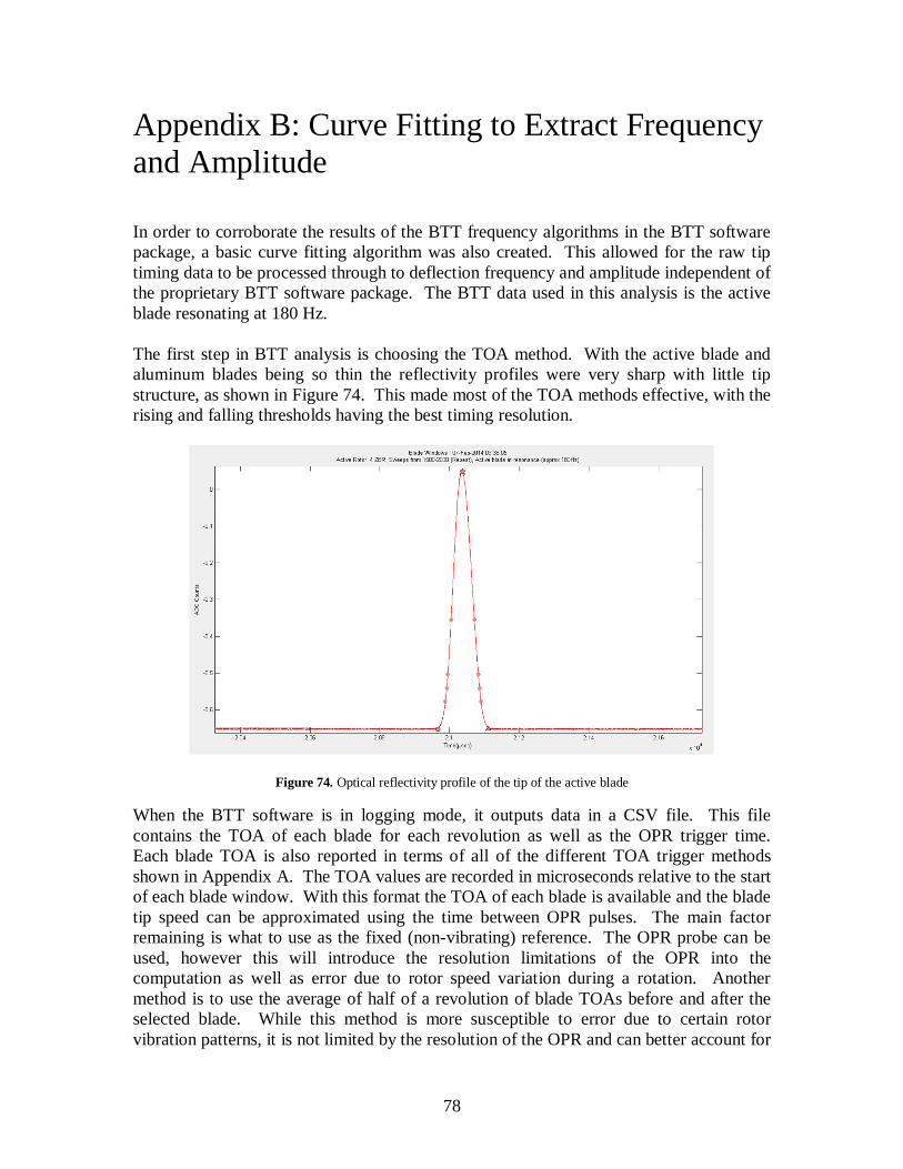
78

Appendix B: Curve Fitting to Extract Frequency and Amplitude In order to corroborate the results of the BTT frequency algorithms in the BTT software package, a basic curve fitting algorithm was also created. This allowed for the raw tip timing data to be processed through to deflection frequency and amplitude independent of the proprietary BTT software package. The BTT data used in this analysis is the active blade resonating at 180 Hz. The first step in BTT analysis is choosing the TOA method. With the active blade and aluminum blades being so thin the reflectivity profiles were very sharp with little tip structure, as shown in Figure 74. This made most of the TOA methods effective, with the rising and falling thresholds having the best timing resolution.

Figure 74. Optical reflectivity profile of the tip of the active blade

When the BTT software is in logging mode, it outputs data in a CSV file. This file contains the TOA of each blade for each revolution as well as the OPR trigger time. Each blade TOA is also reported in terms of all of the different TOA trigger methods shown in Appendix A. The TOA values are recorded in microseconds relative to the start of each blade window. With this format the TOA of each blade is available and the blade tip speed can be approximated using the time between OPR pulses. The main factor remaining is what to use as the fixed (non-vibrating) reference. The OPR probe can be used, however this will introduce the resolution limitations of the OPR into the computation as well as error due to rotor speed variation during a rotation. Another method is to use the average of half of a revolution of blade TOAs before and after the selected blade. While this method is more susceptible to error due to certain rotor vibration patterns, it is not limited by the resolution of the OPR and can better account for

79

rotor speed variations during a rotation. For this analysis this second method was used. The resulting deflection vs. time plot is shown for the active blade with data from all probes combined in Figure 75 (approximately 28 seconds of data). Only the first couple seconds of data, shown highlighted in red, was imported for this analysis.

Figure 75. Deflection (mm) vs. time (s) for the active blade with deflection data from all probes combined

A summary of the blade TOA to deflection conversion is shown in Figure 76.

Figure 76. Example method for converting individual probe blade TOA data to combined blade deflection data

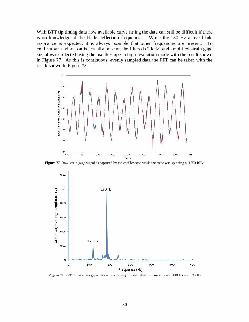
80

With BTT tip timing data now available curve fitting the data can still be difficult if there is no knowledge of the blade deflection frequencies. While the 180 Hz active blade resonance is expected, it is always possible that other frequencies are present. To confirm what vibration is actually present, the filtered (2 kHz) and amplified strain gage signal was collected using the oscilloscope in high resolution mode with the result shown in Figure 77. As this is continuous, evenly sampled data the FFT can be taken with the result shown in Figure 78.

Figure 77. Raw strain gage signal as captured by the oscilloscope while the rotor was spinning at 1650 RPM

Figure 78. FFT of the strain gage data indicating significant deflection amplitude at 180 Hz and 120 Hz

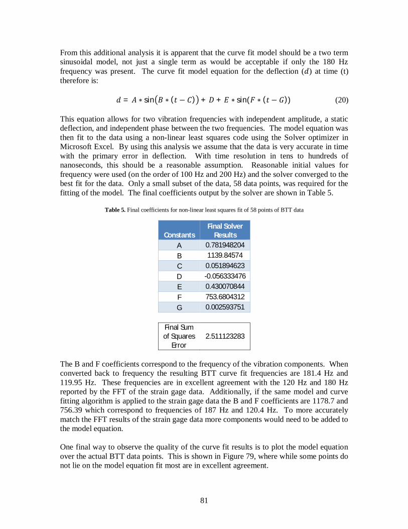
81

From this additional analysis it is apparent that the curve fit model should be a two term sinusoidal model, not just a single term as would be acceptable if only the 180 Hz frequency was present. The curve fit model equation for the deflection (푑) at time (t) therefore is:

푑 = 퐴 ∗ sin 퐵 ∗ (푡 − 퐶) + 퐷 + 퐸 ∗ sin (퐹 ∗ (푡 − 퐺)) (20)

This equation allows for two vibration frequencies with independent amplitude, a static deflection, and independent phase between the two frequencies. The model equation was then fit to the data using a non-linear least squares code using the Solver optimizer in Microsoft Excel. By using this analysis we assume that the data is very accurate in time with the primary error in deflection. With time resolution in tens to hundreds of nanoseconds, this should be a reasonable assumption. Reasonable initial values for frequency were used (on the order of 100 Hz and 200 Hz) and the solver converged to the best fit for the data. Only a small subset of the data, 58 data points, was required for the fitting of the model. The final coefficients output by the solver are shown in Table 5.

Table 5. Final coefficients for non-linear least squares fit of 58 points of BTT data

Constants Final Solver

Results A 0.781948204 B 1139.84574 C 0.051894623 D -0.056333476 E 0.430070844 F 753.6804312 G 0.002593751

Final Sum of Squares

Error 2.511123283

The B and F coefficients correspond to the frequency of the vibration components. When converted back to frequency the resulting BTT curve fit frequencies are 181.4 Hz and 119.95 Hz. These frequencies are in excellent agreement with the 120 Hz and 180 Hz reported by the FFT of the strain gage data. Additionally, if the same model and curve fitting algorithm is applied to the strain gage data the B and F coefficients are 1178.7 and 756.39 which correspond to frequencies of 187 Hz and 120.4 Hz. To more accurately match the FFT results of the strain gage data more components would need to be added to the model equation. One final way to observe the quality of the curve fit results is to plot the model equation over the actual BTT data points. This is shown in Figure 79, where while some points do not lie on the model equation fit most are in excellent agreement.

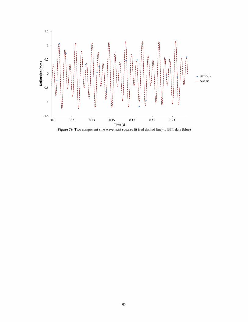
82

Figure 79. Two component sine wave least squares fit (red dashed line) to BTT data (blue)