Market Valuation and Acquisition Quality: Empirical...
47
Market Valuation and Acquisition Quality: Empirical Evidence Christa H. S. Bouwman Case Western Reserve University Kathleen Fuller University of Mississippi Amrita S. Nain McGill University Existing research shows that significantly more acquisitions occur when stock markets are booming than when markets are depressed. Rhodes-Kropf and Viswanathan (2004) hy- pothesize that firm-specific and market-wide (mis-)valuations lead to an excess of mergers, and these will be value destroying. This article investigates whether acquisitions occurring during booming markets are fundamentally different from those occurring during depressed markets. We find that acquirers buying during high-valuation markets have significantly higher announcement returns but lower long-run abnormal stock and operating performance than those buying during low-valuation markets. We investigate possible explanations for the long-run underperformance and conclude it is consistent with managerial herding. (JEL G34) A sizeable stream of theoretical and empirical research on mergers and acquisi- tions (M&A) reveals that takeover activity comes in waves; announcement-day returns are significantly positive for target shareholders but may be significantly positive or negative for bidder shareholders depending on the mode of acqui- sition, method of payment, and type of target; and postacquisition returns to acquiring shareholders are higher for cash offers and tender offers than for stock offers and mergers. 1 More recent research explores the possible link between The authors thank an anonymous referee and Matt Spiegel for helpful suggestions, and Arnoud Boot, Sreedhar Bharath, Sugato Bhattacharyya, Jayant Kale, Gautam Kaul, E. Han Kim, Marc Lipson, Jeffry Netter, David Robinson, Nejat Seyhun, Anjan Thakor, “Vish” Viswanathan, Guojun Wu, participants of the University of Michigan Business School Finance Department Brown Bag Seminar, University of Mississippi 2004 seminar series, University of Missouri–Kansas City 2004 seminar series, the 2002 Estes Park Conference, and the 2003 Financial Management Association Conference for useful comments. The 3rd author thanks the Institut de Finance Math´ ematique de Montreal for research support. Address correspondence to A. S. Nain, McGill University, 1001 Sherbrooke Street West, Montreal, Quebec H3A 1G5, Canada; telephone: 514-398-8440; email: [email protected]. 1 For a discussion of merger waves, see Andrade, Mitchell, and Stafford (2001), and Holmstrom and Kaplan (2001). For evidence on announcement-day returns and postacquisition returns, see Asquith, Bruner, and Mullins (1983); Jensen and Ruback (1983); Dennis and McConnell (1986); Bradley, Desai, and Kim (1988); Franks, Harris, and Titman (1991); Agrawal, Jaffe, and Mandelker (1992); Loughran and Vijh (1997); Rau and Vermaelen (1998); Bruner (2002); and Fuller, Netter, and Stegemoller (2002). C The Author 2007. Published by Oxford University Press on behalf of The Society for Financial Studies. All rights reserved. For permissions, please email: [email protected]. doi:10.1093/rfs/hhm073 Advance Access publication December 11, 2007
Transcript of Market Valuation and Acquisition Quality: Empirical...

Market Valuation and Acquisition Quality:Empirical Evidence
Christa H. S. BouwmanCase Western Reserve University
Kathleen FullerUniversity of Mississippi
Amrita S. NainMcGill University
Existing research shows that significantly more acquisitions occur when stock markets arebooming than when markets are depressed. Rhodes-Kropf and Viswanathan (2004) hy-pothesize that firm-specific and market-wide (mis-)valuations lead to an excess of mergers,and these will be value destroying. This article investigates whether acquisitions occurringduring booming markets are fundamentally different from those occurring during depressedmarkets. We find that acquirers buying during high-valuation markets have significantlyhigher announcement returns but lower long-run abnormal stock and operating performancethan those buying during low-valuation markets. We investigate possible explanations forthe long-run underperformance and conclude it is consistent with managerial herding. (JELG34)
A sizeable stream of theoretical and empirical research on mergers and acquisi-tions (M&A) reveals that takeover activity comes in waves; announcement-dayreturns are significantly positive for target shareholders but may be significantlypositive or negative for bidder shareholders depending on the mode of acqui-sition, method of payment, and type of target; and postacquisition returns toacquiring shareholders are higher for cash offers and tender offers than for stockoffers and mergers.1 More recent research explores the possible link between
The authors thank an anonymous referee and Matt Spiegel for helpful suggestions, and Arnoud Boot, SreedharBharath, Sugato Bhattacharyya, Jayant Kale, Gautam Kaul, E. Han Kim, Marc Lipson, Jeffry Netter, DavidRobinson, Nejat Seyhun, Anjan Thakor, “Vish” Viswanathan, Guojun Wu, participants of the University ofMichigan Business School Finance Department Brown Bag Seminar, University of Mississippi 2004 seminarseries, University of Missouri–Kansas City 2004 seminar series, the 2002 Estes Park Conference, and the2003 Financial Management Association Conference for useful comments. The 3rd author thanks the Institutde Finance Mathematique de Montreal for research support. Address correspondence to A. S. Nain, McGillUniversity, 1001 Sherbrooke Street West, Montreal, Quebec H3A 1G5, Canada; telephone: 514-398-8440;email: [email protected].
1 For a discussion of merger waves, see Andrade, Mitchell, and Stafford (2001), and Holmstrom and Kaplan (2001).For evidence on announcement-day returns and postacquisition returns, see Asquith, Bruner, and Mullins (1983);Jensen and Ruback (1983); Dennis and McConnell (1986); Bradley, Desai, and Kim (1988); Franks, Harris, andTitman (1991); Agrawal, Jaffe, and Mandelker (1992); Loughran and Vijh (1997); Rau and Vermaelen (1998);Bruner (2002); and Fuller, Netter, and Stegemoller (2002).
C© The Author 2007. Published by Oxford University Press on behalf of The Society for Financial Studies.All rights reserved. For permissions, please email: [email protected]:10.1093/rfs/hhm073 Advance Access publication December 11, 2007

The Review of Financial Studies / v 22 n 2 2009
M&A activity and stock prices. Jovanovic and Rousseau (2001) show that peri-ods of high merger activity are correlated with high market valuations.2 Rhodes-Kropf and Viswanathan (2004) develop a model in which firm-specific andmarket-wide misvaluations can cause merger waves. Shleifer and Vishny (2003)model the impact of market valuations on the decision to acquire, the methodof payment, acquirer performance, and the occurrence of merger waves. Con-sistent with these theories, Rhodes-Kropf, Robinson, and Viswanathan (2005)find strong empirical evidence that market (mis-)valuation affects merger ac-tivity. Moreover, there is plenty of anecdotal evidence, including the followingquote, that acquisition decisions are influenced by market valuations.
Why did CEOs do so many deals . . . ? The bull market was a big reason,of course. Executives were brimming with confidence and rich stocks.(Business Week, 14 October 2002, p. 68)
Theory suggests that market valuations may affect not only merger activity,but also the quality of completed deals. Using a model where stock prices haveboth a firm-specific and a market-/industry-wide component, Rhodes-Kropfand Viswanathan (2004) show that (mis-)valuation leads to ex post mistakesthat are correlated with (mis-)valuation at the market/industry level. When mar-ket/industry valuation is low, targets will accept bids only if synergy estimatesoutweigh the negative information in the stock price. When market/industryvaluation is high, targets filter out too little of the market-wide effect, and hencebids tend to appear more attractive and targets are more prone to accept. Thus,from the acquiring-firm shareholders’ perspective, the best deals (on average)are initiated when markets are depressed while worse deals are initiated whenmarkets are booming. Goel and Thakor (2005) also predict that mergers un-dertaken during bull markets involve smaller synergies than those undertakenduring bear markets, and hence will be of lower quality. If deals initiated whenmarkets are booming in fact do create less value for acquiring-firm shareholdersthan deals initiated when markets are depressed, managers may want to refrainfrom undertaking acquisitions during boom periods. The goal of this article isto shed light on these issues by empirically addressing the following question:Are acquisitions that are announced when the market is booming fundamen-tally different from those that are initiated during market troughs? Specifically,we want to investigate whether acquisitions undertaken during booming stockmarkets are of poorer quality than those undertaken during depressed markets,and if so, why?
Using a sample of 2944 acquisitions announced between 1 January 1979and 31 December 2002, we examine if fundamental quality differences exist
2 As noted in Nelson (1959), the idea that stock prices influence merger activity is not new. In a related paper,Jovanovic and Braguinsky (2004) show in a rational setting that acquisitions undertaken during periods whenaverage project quality is high generate greater postacquisition losses than those undertaken when average projectquality is low. To the extent that average project quality is higher when markets are booming, this suggests thatpostacquisition losses are greater for acquisitions announced in booming markets.
634

Market Valuation and Acquisition Quality
between acquisitions announced when market valuations are high and thoseannounced when market valuations are low. We split our sample period intotimes of high, neutral, and low market valuations, and compare the performanceof firms that announce acquisitions under those different market circumstances.We use several stock and operating performance measures. We examine acquir-ing firms’ short-run stock performance (three-day cumulative abnormal returns(CARs)) and long-run stock performance (two-year buy-and-hold abnormal re-turns (BHARs) and calendar-time portfolio returns) to see whether the market’sinitial reaction is consistent with the acquirers’ long-run stock performance.We also analyze long-run operating performance (two-year abnormal return onoperating income (AROOI)) of acquirers to find out whether it is consistentwith our stock performance results. We examine the performance of high-,neutral-, and low-market acquisitions in a univariate setting and in a multivari-ate regression framework in which we control for other factors that may affectacquisition performance, including method of payment, acquisition type (ten-der/merger), the relative size of the acquisition, and acquirer market-to-book(M/B). Both approaches yield similar results.
The definition of what constitutes a market boom or trough is critical. Weuse seven alternative methods to classify time periods into high-, neutral-, andlow-valuation markets and refer to deals initiated during those periods as high-,neutral-, and low-market acquisitions, respectively. Our main classificationmethod is based on the price-earnings (P/E) ratio of the S&P 500 index. Sincethe market P/E has steadily increased over our sample period, we use a de-trended version rather than the actual market P/E to ensure that low-valuation(high-valuation) markets do not simply correspond to the 1st (2nd) half of oursample period. Alternative classification methods use the level of the S&P 500index, the M/B ratio of the overall market, and the M/B ratio of the acquirer’sindustry. Our results are generally similar. One potential concern is that ourmarket valuation measures simply reflect firm valuation; however, our resultshold even after explicitly taking firm valuations into account.
Our main findings are as follows. Bidder announcement returns are in-significantly negative for acquisitions initiated in high-valuation markets butsignificantly negative for deals announced in low-valuation markets, and thedifference between the two is significant. Interestingly, although firms that ac-quire when markets are booming produce significantly higher announcementreturns for their shareholders than do firms that acquire when markets are de-pressed, they generate significantly lower long-run abnormal stock performancefor their shareholders, as measured by BHARs and calendar-time abnormal re-turns.3 While this pattern may also be consistent with short-term momentumfollowed by long-run stock price reversals, we show that the underperformanceof high-market acquisitions is not driven by reversals. Furthermore, high-market
3 The BHAR results hold regardless of whether the announcement month return is included in the analysis. Infact, our results are even stronger if we include the announcement month returns: the positive performance oflow-market stock acquisitions is significant in this case.
635

The Review of Financial Studies / v 22 n 2 2009
acquirers have significantly lower (i.e., more negative) long-run operating per-formance, as measured by AROOIs, than that of low-market acquirers. Thus,our main findings suggest that low-market acquisitions are fundamentally dif-ferent from high-market acquisitions.
Another interesting finding of our article concerns previously documentedevidence that acquisitions made with cash deliver positive long-run abnormalstock returns for acquirers (see Loughran and Vijh, 1997; Rau and Vermaelen,1998). We find that while cash acquisitions undertaken in the 1980s generatedsignificantly positive long-run abnormal stock returns for bidder sharehold-ers, cash acquisitions undertaken in the 1990s produced significantly negativelong-run abnormal returns. This poor performance of cash acquisitions in the1990s was driven by the significant underperformance of high-market cashacquisitions that accounted for 60% of all cash acquisitions in that decade. Theexperience of high-market cash acquirers in the 1990s suggests that when stockprices are soaring, making cash offers may destroy shareholder value.
In the 2nd part of the article, we explore reasons why high-market acquirersunderperform relative to low-market acquirers in the long run. We examine threepossible explanations: overpayment, market timing, and managerial herding.We discuss these in turn. First, managers may be overpaying for targets duringhigh-valuation markets. However, we do not find evidence consistent withoverpayment: the average bid premium is significantly lower in high-valuationmarkets than in low-valuation markets.
The 2nd explanation for the underperformance of high-market acquirers weexplore is market timing. During stock market booms, the enthusiasm to paywith overvalued stock may increase the number of stock acquisitions, and sig-naling theory suggests that these are likely to experience subsequent stock-pricecorrections. Consistent with this, our data show that there are far more stockacquisitions during high-valuation markets than during low-valuation markets.However, when we partition high-market acquirers based on whether they an-nounce a stock acquisition when their stock price is close to an annual high(market timers), we find that market timers have significantly higher BHARsand insignificantly higher calendar-time returns. Thus, it does not seem thatmarket timing can explain why high-market acquirers perform relatively poorly.Four additional factors suggest market timing is not a sufficient explanationfor our results. First, we find that the operating performance of high-marketacquirers is also significantly less than that of low-market acquirers. Second,the operating performance of market timers is statistically indistinguishablefrom that of acquirers who do not time the market. Third, cash acquisitionsannounced during high-valuation markets (39% of high-market acquisitions)also significantly underperform in the long run: these acquisitions are not at-tempts to time the market and do not signal overvaluation of acquirer stock.Fourth, the performance of high-market cash acquirers whose stock prices areclose to a recent peak is not significantly different from that of high-marketcash acquirers whose stock prices are not close to a peak.
636

Market Valuation and Acquisition Quality
The 3rd explanation for the underperformance of high-market acquirers weinvestigate is the possibility of managerial herding during merger waves thataccompany booming stock markets. Existing models of herding suggest thatfirms who move later in a merger wave are likely to perform poorly relativeto firms that move earlier. Persons and Warther (1997) present a fully rationalmodel that predicts that innovation waves tend to end on a sour note becausefirms stop adopting a technology only after observing the poor experienceof recent adopters. Rhodes-Kropf and Viswanathan (2004) also suggest thatmerger waves end only after the market learns from the bad experience ofprevious acquirers. According to these models, acquisitions occurring late ina merger wave are more likely to be value destroying. Other models (see, forexample, Banerjee, 1992; Bikhchandani, Hirshleifer, and Welch, 1998) suggestthat if a handful of firms consecutively adopt an action, subsequent firms willignore their own private signals about the value of that action and defer to theactions of predecessors. As a result, if the state of the world is stochasticallychanging, these models also seem to suggest that, by ignoring their own signals,late movers are likely to make unprofitable acquisitions even though theyhave the benefit of information implicit in the actions of predecessors. Thus,if managerial herding is the explanation for the underperformance of high-market acquisitions, then this underperformance is likely to be driven by firmsthat acquire later in a high-valuation merger wave.
We perform various tests and conclude that managerial herding is a likelyexplanation for the underperformance of high-market acquirers. We divide thesample of acquirers buying during high-valuation markets into early and latemovers, and find that early acquirers show no abnormal stock performance,as measured by BHARs, in the two years following the acquisition announce-ment, while late acquirers underperform. Difference-in-means tests indicatethat higher BHARs than late movers. These results hold for both cash andstock acquisitions, and cannot be explained by industry effects or observabledifferences in acquirer and target characteristics. We also find that the calendar-time returns and operating performance of early acquirers are both significantlybetter than those of late acquirers during high-valuation periods. Recognizingthat merger waves are a phenomenon of booming stock markets, we repeat ouranalysis for stock acquisitions announced during low-valuation markets andexpect to see no difference in the performance of early and late movers. Our(stock) performance findings confirm this. An alternative approach where wesplit high-market acquirers into early, middle, and late movers yields similarresults: early movers show significantly better performance than do middleand late movers. On the basis of these results, we conclude that the overallunderperformance of high-market acquirers is attributable to firms that acquirelater in high-valuation markets and this underperformance is consistent withthe existence of managerial herding.
Our article is related to Loughran and Vijh (1997), Rau and Vermaelen(1998), Ang and Cheng (2006), Dong et al. (2006), and Rhodes-Kropf,
637

The Review of Financial Studies / v 22 n 2 2009
Robinson, and Viswanathan (2005). Loughran and Vijh (1997) find that thelong-run performance of acquirers using stock is worse than that of acquirersusing cash and that tender offers have significantly positive long-run returnswhile mergers have significantly negative long-run returns. Rau and Vermaelen(1998) find that the acquirer’s M/B at the time of the acquisition affects itslong-term stock performance; specifically, firms with low book-to-market ra-tios underperform in the long run. In this article, we control for the methodof payment and the mode of acquisition (as in Loughran and Vijh, 1997), andfor acquirer M/B (as in Rau and Vermaelen, 1998), and focus on the impact ofmarket-wide valuations on acquirer performance in the short and long run. Angand Cheng (2006) and Dong et al. (2006) provide evidence that market mis-valuation impacts the volume of takeovers and the behavior of participants intakeover contests. In both papers, market valuation is defined on a firm-specificlevel (M/B ratios), whereas we define market valuation as the valuation of themarket as a whole or the valuation of the industry in which an acquirer isactive, while controlling for firm-specific valuations. Finally, Rhodes-Kropf,Robinson, and Viswanathan (2005) examine if firm-specific and market-wide(mis-)valuations cause merger waves. In this article, we are not concerned withthe causes of merger waves.
The rest of the article is organized as follows. Section 1 describes the data,Section 2 discusses our methodology, and Section 3 presents our results.Section 4 examines possible explanations for our results. Robustness issuesare addressed in Section 5. Section 6 summarizes and concludes the article.
1. Data
In this section, we describe our sample, explain our classification into high-,neutral-, and low-valuation markets, and provide summary statistics.
1.1 DescriptionOur sample contains completed tender offers and mergers gathered from theSecurities Data Corporation’s (SDC) US Mergers and Acquisitions Databasethat were announced between 1 January 1979 and 31 December 2002. Weidentify 2944 acquisitions that meet the following conditions:
1. The acquirer is a US firm listed on the NYSE, NASDAQ, or AMEX.2. The target is not a subsidiary.4
3. Daily acquirer return data are available for three days around the an-nouncement date and the following acquirer data are available for twoyears following the acquisition: market equity (as of June of each year),the book-to-market ratio (as of December of each year), and monthly returndata.
4 Hansen and Lott (1996) and Fuller, Netter, and Stegemoller (2002) justify the exclusion of subsidiary acquisitions.
638

Market Valuation and Acquisition Quality
4. The transaction value is $50 million or more.5. The acquirer obtains at least 50% of the shares of the target.6. The closing share price of the acquirer for the month before the announce-
ment is at least $3 (see Loughran and Vijh, 1997). This eliminates firmsthat are very small or in distress.
7. The method of payment is cash, stock, or a mixture of the two. As in Fuller,Netter, and Stegemoller (2002) and Heron and Lie (2002), we define a cashacquisition as any acquisition in which the total transaction value was paidin cash, nonconvertible debt, or nonconvertible preferred stock. We definea stock acquisition as any acquisition in which the total transaction valuewas paid in common stock and options, warrants, rights, or convertibledebt. Acquisitions with some combination of cash and stock are defined asmixed-payment acquisitions.
1.2 Classification of high-, neutral-, and low-valuation marketsWe want to examine whether acquisitions announced in high-valuation mar-kets are fundamentally different from acquisitions announced in low-valuationmarkets. Therefore, how we measure the market’s valuation is very important.To ensure that our conclusions are not based on one particular definition ofmarket valuation, we use seven alternative definitions. Here we discuss ourbase specification, which is based on the P/E ratio of the S&P 500 and usesmonthly data. Alternative definitions, which use quarterly data, or are based onthe level of the S&P 500, the M/B ratio of the overall stock market, or the M/Bratio of the industry in which the acquirer operates, are covered in Section 5.2.
Our base specification classifies the stock market in a particular month as ahigh-, neutral-, or low-valuation market based on the P/E ratio of the S&P 500(and we refer to acquisitions that were announced during that month as high-,neutral-, or low-market acquisitions).5 At first glance, it seems as if we couldsimply use the market’s actual P/E ratio in a particular month to classify themarket. However, the P/E ratio of the market has trended upward over time,and hence this approach would lead us to classify all acquisitions that occurredin the 1st half of the sample period (1979–1991) as low-market acquisitions,and all acquisitions that were announced in the 2nd half (1992–2002) as high-market acquisitions. Since the 1980s contained a merger wave and only thelatter half of the 1990s is commonly referred to as a merger wave (see Andrade,Mitchell, and Stafford, 2001), our approach must avoid this problem.
First, we detrend the market P/E by removing the best straight-line fit fromthe P/E of the month in question and the five preceding years.6 Second, eachmonth is categorized as above (below) average if the detrended market P/E ofthat month was above (below) this past five-year average. Third, the top halfof the above-average months are then classified as high-valuation markets and
5 We thank Bob Shiller for providing the P/E data on his Web site (www.irrationalexuberance.com/index.htm).
6 Our results are robust to reasonable changes in the length of the historical data used to detrend the P/E ratio.
639

The Review of Financial Studies / v 22 n 2 2009
the bottom half of the below-average months are classified as low-valuationmarkets. All other months are classified as neutral-valuation markets.
Using this approach, half of all months are classified as neutral-valuationmarkets, while high-valuation and low-valuation markets combined constitutethe other half. Alternatively, one could argue that the number of high-, neutral-,and low-valuation markets should be the same, or that markets should onlybe classified as high-valuation (low-valuation) if the detrended P/E ratio in aparticular month is sufficiently far (e.g., 0.5 standard deviation) above (below)the past five-year average. We show in Section 5.2 that our results are robust tothese alternative specifications.
1.3 Summary statisticsFrom January 1979 to December 2002, we find 85 high-valuation, 59 low-valuation, and 144 neutral-valuation markets.7 Table 1 shows that there areslightly more acquisitions during high-valuation markets than during low-valuation markets. In terms of total deal value, 42% (33%) of all acquisitiondollars are spent in high- (low-) valuation markets. Moreover, about 46% ofhigh-market acquisitions are for stock (corresponding to 66% of total deal valuein high-valuation markets) but only about 37% of low-market acquisitions arefor stock (corresponding to 55% of total deal value in low-valuation markets).Figure 1 shows how acquisitions in our sample are spread out over time.
2. Methodology
We examine the performance of acquisitions announced in high-, neutral-, andlow-valuation markets by studying the short-run stock performance, long-runstock performance, and long-run operating performance in a univariate settingand in a multivariate framework in which we control for other factors that mayaffect postacquisition performance. Section 2.1 discusses our announcementreturn measure: three-day CARs. Section 2.2 deals with long-run stock per-formance. Given well-known controversies surrounding the measurement oflong-run stock returns, we use two alternative measures: two-year BHARs andcalendar-time portfolio returns. Section 2.3 describes our long-run operatingperformance measure: two-year AROOI. Section 2.4 presents our multivariateframework.
2.1 Announcement returnsFollowing Brown and Warner (1985), we use the modified market model toestimate abnormal returns. We do not use the market model because the pres-ence of frequent acquirers in our sample suggests a high probability of other
7 Our sample period spans 24 years and thus contains 288 months. As explained in Section 1.2, our base approachclassifies half of all months as neutral-valuation markets. Of the remaining months, 85 (59) are classified ashigh-valuation (low-valuation) markets, which implies that in 60% (40%) of all months, the detrended P/E ratiowas above (below) the past five-year average.
640

Market Valuation and Acquisition Quality
Tabl
e1
Sum
mar
yst
atis
tics
Num
ber
ofM
ean
mar
ket
Mea
ntr
ansa
ctio
nM
edia
nm
arke
tM
edia
ntr
ansa
ctio
nTo
tald
eal
%of
tota
l%
ofto
taln
umbe
rac
quis
ition
seq
uity
($m
illio
n)va
lue
($m
illio
n)eq
uity
($m
illio
n)va
lue
($m
illio
n)va
lue
($m
illio
n)de
alva
lue
ofac
quis
ition
s
AL
Lac
quis
ition
s2,
944
14,3
8187
02,
009
159
2,56
0,89
010
0.0
100.
0H
igh-
mar
keta
cqui
sitio
ns1,
090
9,12
798
91,
949
161
1,07
8,40
142
.137
.0N
eutr
al-m
arke
tacq
uisi
tions
850
12,7
2876
41,
642
140
649,
286
25.4
28.9
Low
-mar
keta
cqui
sitio
ns1,
004
21,4
8683
02,
633
170
833,
203
32.5
34.1
Cas
hac
quis
ition
s1,
156
12,7
0239
21,
802
125
453,
632
17.7
39.3
Stoc
kac
quis
ition
s1,
269
18,9
031,
207
2,65
420
41,
531,
964
59.8
43.1
Mix
edpa
ymen
tacq
uisi
tions
519
7,06
71,
108
1,23
316
757
5,29
522
.517
.6
Hig
h-m
arke
tcas
hac
quis
ition
s42
18,
528
351
1,65
012
214
7,65
913
.738
.6H
igh-
mar
kets
tock
acqu
isiti
ons
499
11,0
781,
421
2,81
522
070
9,08
665
.845
.8H
igh-
mar
ketm
ixac
quis
ition
s17
04,
883
1,30
41,
295
197
221,
656
20.6
15.6
Neu
tral
-mar
ketc
ash
acqu
isiti
ons
305
7,66
743
21,
549
122
131,
873
20.3
35.9
Neu
tral
-mar
kets
tock
acqu
isiti
ons
395
19,0
6393
22,
009
166
368,
297
56.7
46.5
Neu
tral
-mar
ketm
ixac
quis
ition
s15
06,
335
994
982
129
149,
115
23.0
17.6
Low
-mar
ketc
ash
acqu
isiti
ons
430
20,3
6040
52,
723
132
174,
099
20.9
42.8
Low
-mar
kets
tock
acqu
isiti
ons
375
29,1
451,
212
4,03
523
145
4,58
154
.637
.4L
ow-m
arke
tmix
acqu
isiti
ons
199
9,48
51,
028
1,55
217
120
4,52
424
.519
.8
Thi
sta
ble
show
sth
eac
quir
er’s
mar
ketv
alue
ofeq
uity
and
the
tran
sact
ion
valu
eof
the
acqu
isiti
on.T
hesu
mm
ary
stat
istic
sar
eba
sed
onou
rsam
ple
of29
44ac
quis
ition
s.A
cqui
sitio
nsar
ein
clud
edin
this
sam
ple
ifth
eac
quir
eris
aU
Sfir
mlis
ted
onth
eN
YSE
,AM
EX
,or
NA
SDA
Q;s
uffic
ient
Com
pust
atan
dC
RSP
data
are
avai
labl
e;th
eta
rget
isno
tasu
bsid
iary
;th
etr
ansa
ctio
nva
lue
is$5
0m
illio
nor
mor
e;th
eac
quir
erob
tain
sat
leas
t50%
ofth
esh
ares
ofth
eta
rget
;the
clos
ing
pric
eof
the
acqu
irer
for
the
mon
thbe
fore
the
anno
unce
men
tis
atle
ast$
3;an
dth
em
etho
dof
paym
enti
sca
sh,s
tock
,or
am
ixtu
reof
the
two.
Usi
ngm
onth
lyda
tafr
om19
74to
2002
,eac
hm
onth
from
Janu
ary
1979
toD
ecem
ber
2002
iscl
assi
fied
asa
high
-(l
ow-)
valu
atio
nm
arke
tif
the
detr
ende
dm
arke
tP/
Eof
that
mon
thbe
long
sto
the
top
(bot
tom
)ha
lfof
all
detr
ende
dP/
Es
abov
e(b
elow
)th
epa
stfiv
e-ye
arav
erag
e.A
llot
her
mon
ths
are
clas
sifie
das
neut
ral-
valu
atio
nm
arke
ts.A
nac
quis
ition
isde
fined
asa
cash
acqu
isiti
onif
the
tota
ltr
ansa
ctio
nva
lue
was
paid
inca
sh,n
onco
nver
tible
debt
,and
/or
nonc
onve
rtib
lepr
efer
red
stoc
k.It
isde
fined
asst
ock
ifth
eto
talt
rans
actio
nva
lue
was
paid
inco
mm
onst
ock
and
optio
ns,w
arra
nts,
righ
ts,o
rco
nver
tible
debt
.
641

The Review of Financial Studies / v 22 n 2 2009
Figure 1The detrended market P/E minus its five-year average, and acquisitions announced in high-valuation (=3),neutral-valuation (=2), and low-valuation (=1) markets over time.
acquisition announcements in the estimation period, and any abnormal returnscaused by these announcements will bias our parameter estimates. We calcu-late daily abnormal returns for a firm by deducting the equally weighted indexreturn from the firm’s return8:
ARit = Rit − RMt , (1)
where Rit is firm i’s daily stock return on date t and RMt is the return for theequally weighted CRSP index on date t. We calculate abnormal returns for athree-day event window around the announcement date (from one day prior tothe announcement date to one day after the announcement date). The CARsare calculated by summing the abnormal returns over the three-day window.
2.2 Long-run stock performance2.2.1 BHARs. Our 1st measure of long-run abnormal stock performanceis the BHAR. Barber and Lyon (1997) and Lyon, Barber, and Tsai (1999)highlight three biases that can cause test statistics to be misspecified in tests oflong-run abnormal performance: rebalancing bias, new-listing or survivor bias,and skewness bias.
To control for the rebalancing bias and the new-listing bias we follow themethodology described in Lyon, Barber, and Tsai (1999) to calculate the long-run returns of the reference portfolio. This method involves first compoundingthe returns on securities constituting the reference portfolio and then summing
8 Results are similar when we deduct a value-weighted index instead.
642

Market Valuation and Acquisition Quality
across securities:
RpT =ns∑
j=1
[∏s+Tt=s (1 + R jt )
]− 1
ns, (2)
where RpT is the reference portfolio return, R jt is the month t simple returnon firm j, ns is the number of securities traded in month s, the beginningperiod of the return calculation, and T is the investment horizon in months.The return on this portfolio represents a passive, equally weighted investmentin all securities constituting the reference portfolio in period s. There is noinvestment in firms listed subsequent to period s, nor is there monthly portfoliorebalancing. Consequently, the reference portfolio return calculated this wayis free of the new-listing and rebalancing biases.9 As in Lyon, Barber, andTsai (1999), we assume that the proceeds of delisted firms are invested inan equally weighted reference portfolio, which is rebalanced monthly. Thus,missing monthly returns are filled in with the mean monthly return of firmsconstituting the reference portfolio.
We calculate long-run abnormal returns as the long-run buy-and-hold returnof a sample firm less the long-run buy-and-hold return of our reference portfolio.This long-run abnormal return is referred to as the BHAR and is calculated as
BHARiT =s+T∏t=s
(1 + Rit ) − 1 − RpT , (3)
where Rit is the month t return for firm i, RpT is the reference portfolio re-turn as calculated in Equation (2), and T is the horizon in months over whichreturns are calculated. The BHAR captures the value of investing in the av-erage sample firm relative to an appropriate benchmark over the horizon ofinterest.
9 Although this method of creating reference portfolios eliminates the new-listing and rebalancing biases, itintroduces a different problem. A sample firm is assigned to an appropriate size and book-to-market portfolioat the time of announcement of the acquisition and subsequently, the abnormal returns of the sample firm aremeasured relative to this group of firms for the entire horizon of interest. Insofar as size and book-to-marketcharacteristics of firms change over time, this method introduces inaccuracies in the size and book-to-marketmatching. We have repeated our analysis with abnormal returns calculated in the “traditional” way, which issusceptible to the new-listing and rebalancing bias but allows better matching of firms to the appropriate size andbook-to-market portfolio. In this method, in each month we first calculate the mean return for each portfolio andthen compound this mean return over the horizon of interest. Specifically, the portfolio return is now calculatedas
RpT =s+T∏t=s
[1 +
∑ntj=1 R jt
nt
]− 1.
Calculating portfolio returns this way allows sample firms to be reassigned to new portfolios if size and book-to-market characteristics change. We allow sample firms to change size and book-to-market portfolios once a year.Since we study postannouncement abnormal stock returns, we must allow for a change in the sample firm’s sizewhen the acquisition is completed. Therefore, in addition to allowing firms to change size and book-to-marketportfolios once a year, we also allow sample firms to switch portfolios at the end of the month in which themerger is completed. Our results are robust to this alternative calculation of portfolio returns.
643

The Review of Financial Studies / v 22 n 2 2009
In Appendix A, we explain in detail how we create reference portfolios bycalculating 50 size and book-to-market portfolios in the spirit of Fama andFrench (1993). Appendix B details how we test for significance: since BHARsare positively skewed (Lyon, Barber, and Tsai, 1999) and event samples areunlikely to consist of independent observations (Mitchell and Stafford, 2000),we draw inference based on block-bootstrapped skewness-adjusted t-statistics.
2.2.2 Calendar-time returns. Our 2nd measure of long-run abnormal stockperformance is the calendar-time return. Mitchell and Stafford (2000) demon-strate the existence of cross-sectional correlation of event firm abnormal returns.They suggest an alternative method of measuring long-run stock price perfor-mance: track the performance of an event portfolio in calendar time relativeto an explicit asset pricing model. The event portfolio is formed each periodto include companies that have completed the event in the prior n periods.By forming event portfolios, any cross-sectional correlations of the individualevent firms will be automatically accounted for in the portfolio variance at eachpoint in calendar time.
For each month from January 1982 to December 2002, we create high- andlow-market event portfolios for each month as follows: the high- (low-) marketevent portfolio consists of all sample firms that announced an acquisition duringany high- (low-) market period within the previous two years.10 Portfolios arerebalanced monthly to drop all companies that reach the end of their two-year period and add all companies that have just announced a transaction. Theportfolio excess returns are regressed on the Fama-French (1993) factors andthe Carhart (1997) momentum factor as follows:
Rp,t − R f,t = ap + bp(Rm,t − R f,t ) + spSMB + h pHML
+ m pPR1YR + ep,t , (4)
where Rp,t is the event portfolio return, (Rm,t – R f,t ) represents excess returnon the market, SMB is the difference between a portfolio of “small” and “big”stocks, HML is the difference between a portfolio of “high” and “low” book-to-market stocks, and PR1YR is the Carhart momentum factor. PR1YR is theequal-weighted average of firms with the highest 30% 11-month returns laggedone month minus the equal-weighted average of firms with the lowest 30% 11-month returns lagged one month.11 The intercept ap captures the event portfolioexcess returns.
To study the difference between the calendar-time returns of high- and low-market event portfolios, we create a dummy variable D that equals one if the
10 The results are qualitatively the same if we use a three-year event horizon as in Mitchell and Stafford (2000).Following Mitchell and Stafford (2000), we exclude multiple observations on the same firm that appear withintwo years of the initial observation.
11 We thank Mark Carhart for giving us the momentum factor data, and Ken French for providing the remainingfactors on his Web site.
644

Market Valuation and Acquisition Quality
event portfolio return is a high-valuation return and zero otherwise. A pooledportfolio regression is estimated as follows:
Rp,t − R f,t = ap + bp(Rm,t − R f,t ) + spSMB + h pHML + m pPR1YR
+ δ1 D + δ2 D × (Rm,t − R f,t ) + δ3 D × SMB
+ δ4 D × HML + δ5 D × PR1YR + ep,t , (5)
where the coefficient δ1 captures the difference between high- and low-marketevent portfolios.
2.3 Long-run operating performanceWe use the AROOI as our operating performance measure. As highlighted byHealy, Palepu, and Ruback (1992), measures of accounting performance canbe affected by both the method of payment and the accounting method.12 Ifan acquisition is financed by a mix of cash and debt (a cash acquisition in ourdefinition), the acquirer’s postacquisition net income will be lower than if theacquirer paid stock. The reason is that net income is calculated after deductingthe cost of debt (interest expense), but before the cost of equity (dividends).If the acquirer chooses purchase accounting instead of pooling accounting, itrestates the assets and liabilities of the target at their current market values(not allowed under pooling accounting), records the difference between theacquisition price and the market value of the target as goodwill, and amortizesit (no goodwill is created under pooling accounting). Thus, the book value ofassets, depreciation, and amortization will generally be higher under purchaseaccounting than under pooling accounting, and net income will be lower. Also,under purchase accounting, earnings are usually lower in the year of mergercompletion because results of the target are only consolidated with those ofthe acquirer from the date of merger completion onward, while under poolingaccounting, results are consolidated from the beginning of the year onward.
We deal with these concerns in the spirit of Healy, Palepu, and Ruback(1992). First, we exclude the year of merger completion, and examine account-ing performance over the two years following the year of merger completion.Second, rather than using net income as the numerator of our performancemeasure, we use operating income before interest, taxes, depreciation, andamortization instead. Third, we use average total assets as the denominator ofour performance measure instead of market value of assets. In studies wherethe goal is to find out whether acquirer performance improves after the acqui-sition, it makes sense to compare pre- and postacquisition performance usingthe market value of assets in the denominator (as is done in Healy, Palepu, andRuback, 1992). In contrast, we want to know whether high-market acquisitionsare different from low-market acquisitions. In our stock-performance study, we
12 Until 30 June 2001, acquirers could choose between pooling and purchase accounting to account for an ac-quisition. FASB Statement 141 ruled out the use of pooling accounting for acquisitions undertaken after thisdate.
645

The Review of Financial Studies / v 22 n 2 2009
find overwhelming evidence that the long-run abnormal stock performance ofhigh-market acquisitions is significantly worse than that of low-market acquisi-tions. Since those conclusions are based on abnormal stock performance—i.e.,the performance of the acquirer relative to its peers—this also suggests that themarket value of assets of high-market acquirers (relative to the market valueof assets of their peers) may be lower than the market value of assets of low-market acquirers (relative to the market value of assets of their peers). Knowndifferences in abnormal stock performance could therefore inflate the abnormaloperating performance for high-market acquisitions (using the market value ofassets in the denominator), and hence bias against finding the result that high-market acquisitions show poorer postacquisition accounting performance thando low-market acquisitions. Therefore, we define operating performance asEBITDA (Compustat #13) normalized by average total assets (Compustat #6)(as used in Loughran and Ritter, 1997). However, to guarantee that our resultsare caused by differences in accounting performance, we control for differ-ences in the method of payment and accounting method in the multivariateregressions (see Section 2.4).
To ensure that our results are compared to the proper benchmark, and are notsimply capturing the mean reversion in operating ratios that has been widelydocumented in the accounting literature, we match each firm in our samplewith a control firm following a methodology in the spirit of Barber and Lyon(1996). The control firm must be listed on AMEX, NYSE, or NASDAQ andmust not have been involved in a takeover (either as a target or an acquirer)during the three years after the acquisition completion date. From that set offirms, we find firms in the same industry as the sample firm that have totalassets between 25 and 200% of the sample firm. If no firm meets these criteria,firms are selected from the set of firms with total assets between 90 and 110%of the sample firm without regard to industry. From the resulting set of firms,we select the control firm with the closest operating performance to that ofthe sample firm in the year of the merger completion. If no firm meets thesecriteria, we select a firm with the closest operating performance to that of thesample firm in the year of the merger completion without regard to industryand size. We define AROOI as the operating performance of the acquirer (asdefined above) minus the operating performance of the control firm.
2.4 Multivariate regression frameworkWe run multivariate regressions to control for various factors that may impactabnormal performance of acquirers and address small sample problems thatcan arise in the univariate analysis where the sample of acquisitions is split intomany subgroups. The dependent variables in our regressions are the three-dayCARs, the two-year BHARs, and the two-year AROOI. We first explain theregression setup for CARs and BHARs. We make some minor changes whendealing with AROOI.
646

Market Valuation and Acquisition Quality
2.4.1 Regression framework for short-run and long-run stockperformance. We estimate the following model:
AR = a0 + a1HighValMktDummy + a2NeutralValMktDummy
+ a3CashDummy + a4MixedPaymentDummy + a5TenderDummy
+ a6LogRelSize + a7HighMBDummy + a8MediumMBDummy
+ a9PoolingDummy + a10PreAnnReturn + a11−12LogRelSize
× PaymentDummy + a13LogRelSize × TenderDummy
+ a14−15LogRelSize × MktDummy + a16LogRelSize
× PoolingDummy + a17−20MktDummy × PaymentDummy
+ a21−22MktDummy × TenderDummy + a23−45YearDummy
+ a46−61IndustryDummy (6)
where AR is the three-day CAR or the two-year BHAR. HighValMktDummy(NeutralValMktDummy) equals one if the acquisition was announced in a high-valuation (neutral-valuation) market, and zero otherwise. CashDummy (Mixed-PaymentDummy) is a dummy variable that equals one if the acquisition was paidin cash (a combination of cash and stock) and zero otherwise. TenderDummyequals one if the acquisition was a tender offer and zero otherwise. Previousresearch has demonstrated that the size of an acquisition relative to the acquirerhas an impact on the abnormal returns to the acquiring firm (see, e.g., Asquith,Bruner, and Mullins, 1983; Eckbo, Giammarino, and Heinkel, 1990; Moeller,Schlingemann, and Stulz, 2004). We therefore include LogRelSize, which cap-tures the relative importance of the acquisition and is defined as the logarithmof the transaction value at the time of the acquisition announcement divided bythe acquirer’s market value of equity 30 days prior to the announcement date.13
HighMBDummy (MediumMBDummy) equals one if the acquirer belongs to thehigh (medium) M/B class and zero otherwise. M/B is included because Rau andVermaelen (1998) find that an acquirer’s own valuation affects postacquisitionperformance. As explained in Section 3.3, differences in the accounting methodmay affect the accounting performance of a firm. To allow for the possibilitythat these differences also affect stock returns, we include PoolingDummy, adummy variable that equals one if the acquirer used pooling accounting. Pre-announcement run-ups could affect both our announcement results and ourlong-run stock performance results. To ensure that our findings do not captureshort-term stock price persistence as in Jegadeesh and Titman (1993), we in-clude PreAnnRet, the mean preannouncement stock return (measured from 200days until 31 days prior to the announcement date).
We also include various interaction terms. Because the literature suggeststhat there may be a link between the relative importance of the acquisition
13 To allow for the possibility that actual firm size may matter too, we alternatively include the size of the acquirerand target separately as in Schwert (2000). Results are qualitatively the same using this approach.
647

The Review of Financial Studies / v 22 n 2 2009
and the method of payment choice (see Fuller, Netter, and Stegemoller, 2002),we interact the relative size dummy with the method of payment dummies.Similarly, we interact the relative importance of the acquisition with the modeof acquisition (tender dummy). Since the impact of differences in accountingmethod may be bigger when the target is relatively large, we interact thepooling dummy with the relative size dummy. We also include interaction termsto capture any interaction between the state of the market (high- or neutral-valuation) and the acquirer’s method of payment and mode of acquisition.
We include year dummy variables to control for year-specific effects. Finally,Mitchell and Mulherin (1996) and Andrade, Mitchell, and Stafford (2001) arguethat industry factors are an important determinant of takeover activity andshould be controlled for. We account for industry effects by including industrydummy variables corresponding to the 17 Fama-French industry groupings.14
2.4.2 Regression framework for long-run accounting performance. Ourregression model for long-run accounting performance differs in two respectsfrom the model described above. First, since pre-announcement stock returnsare not likely to affect long-run abnormal accounting performance, we excludePreAnnRet from our AROOI regressions. Second, our AROOI measure explic-itly takes industry effects into account via industry matching; thus, we do notinclude industry dummy variables.
3. Results
In this section, we present the univariate and multivariate results from ourannouncement effect study and our long-run stock and operating performanceanalyses. Figure 2 summarizes the main results.
3.1 Univariate announcement effect studyAs indicated in Table 2, panel A, we find that all acquisitions in our samplehave statistically significant negative returns of −0.48%. This result is drivenby stock acquisitions, which experience significant abnormal performance of−1.47%. Cash acquisitions have a significantly positive abnormal performanceof 0.38% and mixed offers have an insignificantly positive 0.02% return. Fur-ther, we find that tender offers deliver insignificantly negative returns to thebidder of −0.10%, while mergers provide significantly negative returns of−0.53%, driven by the underperformance of stock mergers. These results areconsistent with previous studies.15
Panel B shows that high-market acquirers experience insignificant abnormalreturns of −0.04%, while in panels C and D we see that neutral- and low-marketacquirers suffer significantly negative abnormal returns of −0.06 and −1.31%,respectively. The difference between the three-day CARs for high- and low-market acquirers (1.28%) is significant (panel E). These results suggest that the
14 Results are similar when we use one- or two-digit SIC codes instead.
15 See Bruner (2002) for a comprehensive survey of the studies examining shareholder returns for M&A.
648

Market Valuation and Acquisition Quality
Figure 2Our main results: although high-market acquisitions generate significantly higher announcement returns (CARs)for their shareholders than do low-market acquisitions, their long-run stock performance (BHARs and calendar-time returns) and operating performance (AROOI) are significantly lower.
market is less welcoming of acquisitions during low-valuation markets thanduring high-valuation markets.
When we partition the sample by market valuation and the method of pay-ment, results indicate that cash offers have positive abnormal returns acrossall states of the market (significant for high market acquisitions only), whilestock offers announced in high-, neutral-, and low-valuation markets earn sig-nificantly negative returns. Mixed payment offers provide significantly positivereturns in high-valuation markets, insignificantly positive returns in neutral-valuation markets, and significantly negative returns in low-valuation markets.
Finally, when we control for market valuation and the mode of acquisition, wefind that high-market tender offers experience significantly positive abnormalreturns of 1.46% while neutral- and low-market tender offers suffer significantlynegative abnormal returns of −0.41 and −1.27%, respectively. High-, neutral-,and low-market mergers all experience significantly negative returns, but low-market mergers show the strongest underperformance. These results make itevident that, controlling for mode of acquisition, high-market acquirers farebetter than do low-market acquirers immediately after announcement. Thedifference-in-means test in panel E reinforces this finding: the three-day CARsfor high-market tender offers (mergers) are 2.73% (1.09%) higher than thosefor low-market tender offers (mergers).
In summary, low- and neutral-market acquisitions experience significantlynegative CARs while high-market acquisitions have significantly higher CARs.Thus, the market seems to look more favorably upon acquisition announcementsduring high-valuation markets than during low-valuation markets.
3.2 Long-run stock performance study3.2.1 Univariate BHAR study. Table 3 contains the two-year BHAR re-sults. Note that since we base inference on skewness-adjusted t-statistics, thenormal critical values do not apply. Hence, a coefficient may be significantlypositive (not significant) even though the t-statistic is smaller than (exceeds)
649

The Review of Financial Studies / v 22 n 2 2009
Table 2Three-day CARs
All Cash Stock Mixed payment
Number CAR Number CAR Number CAR Number CAR
Panel A: All acquisitionsAll 2944 −0.48% 1156 0.38% 1269 −1.47% 519 0.02%
(−7.58)a (2.72)a (−14.39)a (0.40)Tender offers 380 −0.10% 310 0.43% 20 −3.92% 50 −1.85%
(−0.94) (1.21) (−1.74)b (−4.50)a
Mergers 2564 −0.53% 846 0.37% 1249 −1.43% 469 0.22%(−7.76)a (2.45)a (−14.29)a (1.89)b
Panel B: High-market acquisitionsAll 1090 −0.04% 421 0.80% 499 −1.08% 170 0.98%
(−1.23) (4.26)a (−7.63)a (3.26)a
Tender offers 124 1.46% 107 1.49% 4 1.05% 13 1.39%(3.96)a (3.62)a (0.64) (1.48)
Mergers 966 −0.23% 314 0.56% 495 −1.10% 157 0.94%(−2.72)a (2.82)a (−7.72)a (2.97)a
Panel C: Neutral-market acquisitionsAll 850 −0.06% 305 0.26% 395 −0.49% 150 0.40%
(−4.56)a (−0.13) (−7.00)a (0.69)Tender offers 124 −0.41% 103 −0.02% 1 4.50% 20 −2.64%
(−2.70)a (−0.90) (1.64) (−5.04)a
Mergers 726 −0.00% 202 0.41% 394 −0.50% 130 0.87%(−3.82)a (0.48) (−7.09)a (2.72)a
Panel D: Low-market acquisitionsAll 1004 −1.31% 430 0.06% 375 −3.01% 199 −1.09%
(−7.50)a (0.36) (−10.50)a (−2.97)a
Tender offers 132 −1.27% 100 −0.23% 15 −5.81% 17 −3.40%(−2.81)a (−0.70) (−2.77)a (−3.54)a
Mergers 872 −1.32% 330 0.15% 360 −2.89% 182 −0.87%(−6.96)a (0.79) (−10.15)a (−2.02)a
Panel E: Differences in mean three-day CARsHigh-market minus low-market acquisition 1.28%
(3.99)a
Cash acquisitions minus stock acquisitions 1.85%(6.30)a
High-market cash minus low-market cash 0.73%(1.72)b
High-market stock minus low-market stock 1.93%(3.46)a
Tender offers minus mergers 0.44%(1.11)
High-market tenders minus low-market tenders 2.73%(2.86)a
High-market mergers minus low-market mergers 1.09%(3.21)a
This table contains three-day CARs for all acquisitions undertaken during high-, neutral-, and low-valuationperiods. Using monthly data from 1974 to 2002, each month from January 1979 to December 2002 is classifiedas a high- (low-) valuation market if the detrended market P/E of that month belongs to the top (bottom) halfof all detrended P/Es above (below) the past five-year average. All remaining months are classified as neutral-valuation markets. CARs for each firm are calculated over days (−1, +1), where day 0 is the announcementday of an acquisition. Z -statistics are provided in parenthesis. Bold font indicates significance at least at the10% level. Superscripts a, b, and c indicate significance at the 1, 5, and 10% levels, respectively.
1.645. Likewise, a coefficient may be significantly negative (not significant)even though the t-statistic exceeds (is smaller than) −1.645. Panel A showsthat acquisitions on average have significantly negative abnormal performance
650

Market Valuation and Acquisition Quality
Table 3Two-year BHARs
All Cash Stock Mixed payment
Number BHAR Number BHAR Number BHAR Number BHAR
Panel A: All acquisitions
All 2944 −7.22% 1156 −0.55% 1269 −13.19% 519 −7.46%(−5.16)a (−0.24) (−5.35)a (−2.85)a
Tender offers 380 1.62% 310 2.17% 20 −24.48% 50 8.68%(0.49) (0.58) (−2.18)b (1.01)c
Mergers 2564 −8.53% 846 −1.54% 1249 −13.01% 469 −9.18%(−5.53)a (−0.60) (−5.23)a (−3.36)a
Panel B: High-market acquisitions
All 1090 −11.32% 421 −9.98% 499 −13.89% 170 −7.12%(−4.62)a (−2.85)a (−3.27)b (−1.66)
Tender offers 124 −5.13% 107 −7.47% 4 −31.64% 13 22.34%(−0.87) (−1.14) (1.48)c
Mergers 966 −12.12% 314 −10.83% 495 −13.75% 157 −9.55%(−4.52)a (−2.58)b (−3.21)b (2.15)b
Panel C: Neutral-market acquisitions
All 850 −6.60% 305 4.95% 395 −16.33% 150 −4.46%(−2.99) (1.35)c (−6.01)a (−0.87)
Tender offers 124 11.52% 103 11.98% 1 −44.15% 20 11.93%(1.87)b (1.73)b (0.86)
Mergers 726 −9.69% 202 1.36% 394 −16.26% 130 −6.98%(−4.33)b (0.34) (−5.97)a (−1.27)c
Panel D: Low-market acquisitions
All 1004 −3.28% 430 4.78% 375 −8.96% 199 10.01%(−1.34) (1.44) (−1.89) (−2.32)c
Tender offers 132 −1.33% 100 2.38% 15 −21.26% 17 −5.59%(−0.22) (0.42) (−1.63) (−0.30)
Mergers 872 −3.58% 330 5.51% 360 −8.45% 182 −10.42%(−1.32) (1.40) (−1.75) (−2.33)b
Panel E: Differences in mean two-year BHARs
High-market minus low-market acquisitions −8.04%(2.60)a
Cash acquisitions minus stock acquisitions −12.64%(−4.47)a
High-market cash minus low-market cash −14.76%(−3.09)a
High-market stock minus low-market stock −4.93%(−0.95)
Tender offers minus mergers 10.15%(2.75)a
High-market tenders minus low-market tenders −3.80%(−0.49)
High-market mergers minus low-market mergers −8.54%(−2.54)a
This table provides post-announcement BHARs for all acquisitions undertaken during high-, neutral-, and low-valuation markets. Using monthly data from 1974 to 2002, each month from January 1979 to December 2002is classified as a high- (low-) valuation market if the detrended market P/E of that month belongs to the top(bottom) half of all detrended P/Es above (below) the past five-year average. All remaining months are classifiedas neutral-valuation markets. Skewness-adjusted t-statistics are provided in parenthesis. Bold font indicatessignificance at least at the 10% level. Superscripts a, b, and c indicate significance at the 1, 5, and 10% levels,respectively. Significance is based on block-bootstrapped critical values.
651

The Review of Financial Studies / v 22 n 2 2009
of −7.22%, tender offers have no abnormal performance, and mergers signifi-cantly underperform by −8.53%.
When we partition our sample on the basis of market valuation and method ofpayment, we find compelling evidence supporting the view that market valua-tions do affect acquirers’ long-run performance. Acquirers buying during high-valuation markets have significant BHARs of −11.32% (panel B), with bothcash and stock acquisitions contributing to this underperformance. High-marketcash acquisitions have significant BHARs of −9.98%, while high-market stockacquisitions have significant BHARs of −13.89%. High-market mixed paymentacquisitions have insignificant abnormal returns. Neutral-market acquisitionsas a whole (panel C) have insignificantly negative abnormal performance.However, neutral-market stock offers significantly underperform while neutral-market cash acquisitions significantly outperform. Low-market acquisitions(panel D) have insignificant BHARs overall as well as for cash and stockacquisitions. Thus, our BHAR results suggest that, on average, high-marketacquisitions destroy value for shareholders in the long run, while low-marketacquisitions do not.
Also notable is the finding that cash acquisitions do not necessarily outper-form the benchmark: cash acquisitions undertaken in high-valuation marketsactually underperform the control portfolio. This appears to be inconsistent withprevious research, notably Loughran and Vijh (1997) and Rau and Vermaelen(1998), which found a pervasive positive abnormal performance of cash acqui-sitions. However, if we split our sample of acquisitions into those undertakenin the 1980s (the sample period used by Loughran and Vijh, and Rau andVermaelen) and those undertaken in the 1990s, our results are consistent withboth studies. We find that in the 1980s, cash acquisitions significantly out-performed the control portfolio by 8.64%. Surprisingly, however, during the1990s, cash acquisitions actually suffered significantly negative abnormal re-turns. This poor performance of cash acquisitions in the 1990s was driven bythe significant underperformance of high-market cash acquisitions (BHAR of−12.74%) that accounted for 60% of all cash acquisitions in the 1990s. Theexperience of high-market cash acquirers in the 1990s leaves an importantlesson—when stock prices are soaring, paying cash for possibly overvaluedtargets may destroy shareholder value.
Finally, we partition the sample by market valuation and mode of acquisition.Panel B of Table 3 shows that mergers undertaken in high-valuation marketshave significant BHARs of −12.12%. This underperformance is evident incash (−10.83%), stock (−13.75%), and mixed payment (−9.55%) mergers.Neutral-market mergers also have significantly negative BHARs (panel C).In contrast, low-market mergers have no abnormal performance (panel D).Our results show that mergers undertaken during high-valuation markets causethe poor performance of mergers as a whole. Tender offers have insignificantreturns during both high- and low-valuation markets but significant, positiveBHARs during neutral-valuation markets (panels B–D).
652

Market Valuation and Acquisition Quality
The impact of market valuation is even more striking when we look at dif-ferences in the magnitude of abnormal performance of high- and low-marketacquisitions. Panel E of Table 3 shows that high-market acquisitions on av-erage significantly underperform low-market acquisitions by −8.04%. Thisdifference is driven by cash deals: high-market cash acquisitions underper-form low-market cash deals by −14.76%. Also note that high-market mergerssignificantly underperform low-market mergers by −8.54%. In contrast, theperformance of high- and low-market tender offers is not significantly dif-ferent. In summary, our BHAR results indicate that high-market acquisitionsperform significantly poorly relative to low-market acquisitions.
The two-year BHARs of high- and low-market acquisitions stand in sharpcontrast to the stock market’s reaction at the time of the acquisition announce-ment. At the time of the announcement, low-market acquirers experiencedsignificantly negative CARs while high-market acquirers showed no abnormalperformance. If the market had anticipated the long-run underperformance ofhigh-market acquirers, what announcement returns should they have experi-enced? To examine this, we begin by assuming that the acquirer’s stock pricetwo years (24 months) after the acquisition announcement is “correct.” Thatis, by the end of the two years, the stock price reflects fundamental value. Wealso assume that in every month, except the announcement month itself, theacquirer’s stock return was exactly equal to the reference portfolio return. Thus,the two-year buy-and-hold return of the acquirer is simply the buy-and-hold re-turn of its size and book-to-market matched portfolio. This assumption imposeszero abnormal returns in all months following the announcement month. Weuse this buy-and-hold return and the stock price in month 24 to back out whatthe stock price should have been at the end of the announcement month itself.This gives us a rough estimate of how the market should have responded shortlyafter the acquisition announcement. We find that for high-market acquisitions,the average return in the announcement month would have to be −36% in orderto eliminate abnormal performance over the two-year horizon.16
3.2.2 Calendar-time results. Table 4 shows the regression results for theevent portfolios. The intercept in the 1st column indicates that acquirers asa whole experience significant abnormal returns of 0.66% per month, whichcorresponds to 15.84% over a period of two years (0.66% × 24). The intercept inthe 2nd (3rd) column shows that high-market (low-market) acquirers experiencesignificant abnormal returns of 0.68% (1.35%) per month, which correspondsto 16.32% (32.40%) over a two-year period.
16 This estimate of the “correct” announcement return for high-market acquisitions is very large in magnitudecompared to the mean two-year BHAR for high-market acquisitions. This difference exists because the buy-and-hold returns of individual firms are very positively skewed compared to the buy-and-hold returns of the benchmarkportfolio returns. The BHARs (which depend on firms’ buy-and-hold returns) are therefore positively skewedrelative to the implied announcement returns (which are calculated using the benchmark portfolio buy-and-holdreturn only). Thus, average BHARs are higher (i.e. less negative) than estimates of the “correct” announcementreturn. Further details are available upon request.
653

The Review of Financial Studies / v 22 n 2 2009
Table 4Long-run stock returns in calendar time: four-factor model portfolio regression results
Estimate (t-value)
Full sample High-market Low-market Pooledevent portfolio event portfolio event portfolio portfolio
Intercept 0.66 0.68 1.35 1.35(7.62)a (3.92)a (5.45)a (6.25)a
(Rmt – R f t ) 1.02 1.06 1.07 1.07(50.11)a (25.74)a (16.64)a (19.07)a
SMB −0.17 −0.09 −0.26 −0.26(−6.44)a (−1.71)c (−3.83)a (−4.39)a
HML −0.15 −0.10 −0.41 −0.41(−4.60)a (−1.60) (−4.83)a (−5.54)a
PR1YR −0.03 −0.06 −0.08 −0.08(−1.86)c (−1.98)b (−2.04)b (−2.34)b
D −0.67(−2.29)b
D × (Rmt – R f t ) −0.01(−0.15)
D × SMB 0.17(2.08)b
D × HML 0.31(3.03)a
D × PR1YR 0.02(0.32)
Number of observations 252 198 141 339Adjusted R2 0.93 0.84 0.79 0.82
This table presents the results of four-factor portfolio regressions. Using monthly data from 1974 to 2002, eachmonth from January 1979 to December 2002 is classified as a high- (low-) valuation market if the detrendedmarket P/E of that month belongs to the top (bottom) half of all detrended P/Es above (below) the past five-yearaverage. All other months are classified as neutral-valuation markets. For each month from 1982 to 2002 we formvalue-weighted portfolios of the following: (i) all sample firms that announced an acquisition in the previous twoyears (1st column); (ii) sample firms that announced acquisitions during any high-valuation period within theprevious two years (2nd column); and (iii) sample firms that announced acquisitions during any low-valuationperiod within the previous two years (3rd column). The portfolio excess returns are regressed on the Fama-Frenchfactors and the Carhart momentum factor as follows:
Rp,t − R f,t = ap + bp(Rm,t − R f,t ) + spSMB + h pHML + PR1YR + ep,t .
The four factors are as follows: zero-investment portfolios representing excess return on the market, (Rm,t – R f,t ),the difference between a portfolio of “small” and “big” stocks, SMB, the difference between a portfolio of “high”and “low” book-to-market stocks, HML, and one-year momentum in stock returns as in Carhart (1997), PR1YR.Abnormal return is captured by the intercept of each regression. The 4th column presents a pooled portfolioregression:
Rp,t − R f,t = ap + bp(Rm,t − R f,t ) + spSMB + h pHML + m pPR1YR + δ1 D + δ2 D × (Rm,t − R f,t )
+ δ3 D × SMB + δ4 D × HML + δ5 D × PR1YR + ep,t ,
where the dummy variable D equals one if the event portfolio return is a high-valuation return and zero otherwise.Difference in the performance of high- and low-valuation acquirers is captured by the coefficient δ1. t-statisticsare provided in parenthesis. Bold font indicates significance at least at the 10% level. Superscripts a, b, and cindicate significance at the 1, 5, and 10% levels, respectively.
In contrast to our BHAR results, both high- and low-market acquirers out-perform in calendar time. Further, the magnitude of calendar-time abnormalreturns is quite different from the BHARs. This difference is not altogethersurprising. Loughran and Ritter (2000) argue that since different methods have
654

Market Valuation and Acquisition Quality
different powers of detecting abnormal performance, there should be differ-ences in abnormal return estimates across different methodologies.
However, since our objective is to highlight any observable differences inthe performance of high- and low-market acquisitions, we check whether thecalendar-time returns of high-market acquirers are significantly different fromthose of low-market acquirers. To do this we run a pooled regression that in-cludes both high- and low-market event returns. The difference in the abnormalperformance of high- and low-market portfolios is captured by a dummy vari-able D that equals one if the event portfolio return is a high-market return andzero otherwise. The last column of Table 4 contains the results of this regres-sion. The coefficient on D, −0.67%, is the difference in the intercepts of thehigh- and low-market event portfolios. The coefficient is significant, suggestingthat low-market acquirers experience significantly higher long-run abnormalreturns than high-market acquirers.
Thus, both calendar-time returns, which account for the cross-correlation ofevent firm returns, and BHARs support the hypothesis that acquirers buyingduring low-valuation markets create significantly more shareholder wealth thanthose buying during high-valuation markets.
3.3 Univariate long-run operating performance studyTable 5 shows our operating performance results, which are consistent withour long-run stock return results as well as with evidence of Healy, Palepu, andRubak (1992). In panel A, we see that the AROOI for the sample is signifi-cantly worse than the benchmark (−1.19%), and that such underperformance iscaused by stock deals, mixed payment deals, and mergers. We find similar re-sults in high-, neutral-, and low-valuation markets (panels B–D), but operatingperformance generally seems better for acquisitions originated in low-valuationmarkets.
The difference between high- and low-market acquisitions becomes evidentwhen we look at the difference-in-medians tests (panel E). The AROOI isa significant 1.72% higher for low-market acquisitions than for high-marketacquisitions. As in the long-run stock return study, there is no significant differ-ence in the operating performance of high- and low-market tenders. However,the AROOI of low-market mergers is a significant 1.98% higher than that ofhigh-market mergers. In contrast to our long-run stock results, the outperfor-mance of low-market acquisitions is driven by stock rather than cash deals:low-market stock acquisitions show 2.15% better AROOI than do high-marketstock acquisitions.
The operating performance results confirm the long-run stock return resultsthat low-market acquirers significantly outperform high-market acquirers.
3.4 Multivariate regression resultsThe multivariate results confirm our previous findings. Table 6, panel A, showsthe short-run results based on the equally weighted index. (Results are very
655

The Review of Financial Studies / v 22 n 2 2009
Table 5Two-year AROOI
All Cash Stock Mixed payment
Number AROOI Number AROOI Number AROOI Number AROOI
Panel A: All acquisitions
All 2596 −1.19% 987 0.09% 1176 −2.76% 433 −0.95%(9.19)a (0.48) (12.42)a (2.74)a
Tender offers 363 0.32% 299 0.32% 17 −0.54% 47 0.33%(1.10) (1.10) (0.24) (0.44)
Mergers 2233 −1.42% 688 −0.02% 1159 −2.78% 386 −1.06%(10.35)a (0.15) (12.48)a (3.05)a
Panel B: High-market acquisitions
All 932 −2.11% 327 −0.50% 472 −3.49% 133 −1.38%(8.91)a (1.16) (10.22)a (2.51)a
Tender offers 119 −0.53% 104 −0.48% 3 −2.01% 12 −0.21%(0.83) (0.78) (0.00)
Mergers 813 −2.40% 223 −0.50% 469 −3.50% 121 −1.41%(9.22)a (0.87) (10.20)a (2.64)a
Panel C: Neutral-market acquisitions
All 785 −1.08% 284 0.49% 368 −2.32% 133 −1.38%(4.82)a (1.31) (7.30)a (1.47)
Tender offers 120 1.47% 99 1.42% 1 32.20% 20 0.31%(2.74)a (2.91)a (0.00)
Mergers 665 −1.59% 185 −0.30% 367 −2.43% 113 −1.43%(6.40)a (0.51) (7.36)a (1.60)
Panel D: Low-market acquisitions
All 879 −0.39% 376 0.19% 336 −1.34% 167 −0.38%(2.06)b (0.72) (3.49)a (0.85)
Tender offers 124 0.07% 96 −0.17% 13 −0.54% 15 1.44%(0.00) (0.20) (0.28) (0.77)
Mergers 755 −0.41% 280 0.23% 323 −1.43% 152 −0.39%(2.22)b (0.96) (3.51)a (1.14)
Panel E: Differences in median two-year AROOI
High-market minus low-market acquisitions −1.72%(−3.27)a
Cash acquisitions minus stock acquisitions 2.85%(9.39)a
High-market cash minus low-market cash −0.70%(−1.04)
High-market stock minus low-market stock −2.15%(−1.69)c
Tender offers minus mergers 1.74%(5.13)a
High-market tenders minus low-market tenders −0.60%(−0.20)
High-market mergers minus low-market mergers −1.98%(−3.28)a
This table shows acquirers’ AROOI averaged over the two years after the completion date for acquisitionsundertaken during high-, neutral, and low-valuation markets. Using monthly data from 1974 to 2002, eachmonth from January 1979 to December 2002 is classified as a high- (low-) valuation market if the detrendedmarket P/E of that month belongs to the top (bottom) half of all detrended P/Es above (below) the past five-yearaverage. Z-statistics for the medians are provided in parenthesis. The Z-statistics for the difference in mediansin panel E are based on the Wilcoxon-Mann-Whitney test and are shown in parenthesis. Bold font indicatessignificance at least at the 10% level. Superscripts a, b, and c indicate significance at the 1, 5, and 10% levels,respectively.
656

Market Valuation and Acquisition Quality
similar using the value-weighted index instead.) It is clear that the announce-ment returns of low M/B, stock-financed mergers that used purchase account-ing and were announced in a low-valuation market are insignificantly negative(−4.80%). The coefficient on the high-valuation market dummy is positiveand significant (3.17%). Thus, as in the univariate tests, acquirers buying inhigh-valuation markets have significantly higher CARs. CARs are significantlylower if the target was large relative to the acquirer (−0.93%). The announce-ment returns are insignificantly lower in a tender offer (−1.05%), when theacquirer used pooling accounting (−1.15%), and do not seem to be affectedby the acquirer’s M/B ratio at the time of the acquisition announcement. TheCARs are significantly higher if the merger was paid for in cash or a mix of cashand stock (5.75 and 3.52%, respectively). CARs are also significantly higherif the acquirer experienced larger preannouncement stock returns, which isconsistent with short-term stock price persistence as in Jegadeesh and Titman(1993).
In panel B, the two-year BHARs of low M/B, stock-financed mergers thatused purchase accounting and were announced in a low-valuation market areinsignificantly negative (−3.46%). They are significantly lower if the mergerwas announced in a high-valuation market (−15.36%), and if the preannounce-ment price run-ups are larger (−22.31%), which is consistent with long-runstock price reversals as in Jegadeesh and Titman (1993). BHARs are signif-icantly higher if it was paid for in cash (30.15%) and if the acquirer usedpooling accounting (13.19%). As in the short-run regressions, acquirer M/Bis not significantly related to long-run abnormal performance.17 The size andsignificance of these coefficients suggest that market-wide valuations are animportant determinant of long-run postacquisition performance even after con-trolling for long-run stock price reversals and acquirer M/B.
In panel C, the two-year AROOI of low M/B, stock-financed mergers thatused purchase accounting and were announced in a low-valuation market are in-significantly positive. As in the stock return regressions, performance is signif-icantly worse if the deal was announced in a high-valuation market (−1.80%).Operating performance is significantly better if the acquirer has high or mediumM/B.
In summary, the results described so far are consistent with the predictionsput forth in the theory that the state of the market in which an acquisitionis initiated affects the long-run performance of the acquirer over and abovethe method of payment used and the acquirer’s own valuation. Insofar as betterlong-run performance reflects smarter business strategies, we find that acquirerswho make acquisitions in low-valuation markets make better decisions than doacquirers who make acquisitions in high-valuation markets.
17 This finding contradicts Rau and Vermaelen’s (1998) result that long-run underperformance of acquirers isdriven by high M/B acquirers. However, if we restrict our sample to the period covered by Rau and Vermaelen(1 January 1980 and 31 December 1991), our two-year BHARs for high and low M/B acquirers are similar tothe bias-adjusted two-year returns of Rau and Vermaelen’s public-targets-only sample.
657

The Review of Financial Studies / v 22 n 2 2009
Table 6Regression analysis of short-run and long-run abnormal returns
Estimate (t-value)
Panel A: dependent Panel B: dependent Panel C: dependentvariable = three-day variable = two-year variable = two-year
CAR BHAR AROOI
Intercept −4.80% −3.46% 0.65%(−1.27) (−0.10) (0.15)
HighValMktDummy 3.17% −15.36% −1.80%(3.72)a (−1.97)b (−1.71)c
NeutralValMktDummy 3.55% −18.02% −1.77%(4.27)a (−2.36)b (−1.73)c
CashDummy 5.75% 30.15% 1.63%(7.11)a (4.08)a (1.58)
MixedPaymentDummy 3.52% 12.02% 1.29%(3.95)a (1.48) (1.12)
TenderDummy −1.05% −5.08% −0.29%(−1.12) (−0.59) (−0.25)
LogRelSize −0.93% −0.97% 0.31%(−5.10)a (−0.59) (1.37)
HighMBDummy 0.13% 0.22% 1.15%(0.27) (0.05) (2.35)b
MediumMBDummy −0.03% 0.68% 1.93%(−0.08) (0.21) (4.50)a
PoolingDummy −1.15% 13.19% 0.48%(−1.56) (1.94)b (0.52)
PreAnnReturn 1.37% −22.31%(2.50)b (−4.43)a
Interaction terms:LogRelSize × PaymentMethod Yes Yes YesLogRelSize × TenderDummy Yes Yes YesLogRelSize × StateOfMarket Yes Yes YesLogRelSize × PoolingDummy Yes Yes YesStateOfMarket × PaymentMethod Yes Yes YesStateOfMarket × TenderDummy Yes Yes YesYear dummy variables Yes Yes YesIndustry dummy variables Yes Yes NoF-statistic 3.21 3.45 7.70Adjusted R2 4.39% 4.84% 10.20%
This table contains ordinary least squares regressions of the acquirer’s three-day CARs (calculated using theCRSP equally weighted index; results are similar when we use the value-weighted index instead), two-yearBHARs, and two-year AROOI on the following variables. HighValMktDummy (NeutralValMktDummy) equalsone if the month in which the acquisition was announced is classified as a high- (neutral-) valuation marketand zero otherwise. Using monthly data from 1974 to 2002, each month from January 1979 to December 2002is classified as a high- (low-) valuation market if the detrended market P/E of that month belongs to the top(bottom) half of all detrended P/Es above (below) the past five-year average. All other months are classified asneutral-valuation markets. CashDummy equals one if the total transaction value was paid in cash, nonconvertibledebt, and/or nonconvertible preferred stock and zero otherwise. MixedPaymentDummy equals one if the totaltransaction value was paid with a combination of cash and stock and zero otherwise. TenderDummy is one if theacquisition was a tender offer and zero otherwise. LogRelSize is the log of the transaction value at the time of theacquisition announcement divided by the acquirer’s market value of equity 30 days prior to the announcement.Acquirers are divided into equal subsamples of high, medium, and low M/B firms based on their M/B ratio onemonth prior to the acquisition announcement. HighMBDummy (MediumMBDummy) equals one if the acquirerbelongs to the high (medium) firm-valuation category. PoolingDummy equals one if the acquirer used poolingaccounting and zero otherwise. PreAnnReturn is the firm’s average stock return measured over [−200,−31].PaymentMethod consists of CashDummy and MixedPaymentDummy, which are described above. StateOfMarketcomprises HighValMktDummy and NeutralValMktDummy, which are also described above. Industry dummyvariables correspond to the 17 Fama-French industry groupings. (Results are similar when we use one-digit ortwo-digit SIC codes instead.) In all panels, the intercept represents a low M/B, stock-financed merger that usedpurchase accounting and was announced in a low-valuation market. t-statistics are provided in parenthesis. Boldfont indicates significance at least at the 10% level. Superscripts a, b, and c indicate significance at the 1, 5, and10% levels, respectively.
658

Market Valuation and Acquisition Quality
4. Possible Explanations
Our findings warrant further research on why acquirers who buy during high-valuation markets underperform relative to those who buy during low-valuationmarkets. In this section, we investigate three potential explanations: overpay-ment, market timing, and managerial herding.
4.1 OverpaymentOne possible explanation for the underperformance of high-market acquirersis that these acquirers overpay. We compare the bid premia paid in high- andlow-valuation markets to see if acquirers who buy in high-valuation marketsdo relatively poorly because they pay more for their purchases. We calculatethe premium paid as (net transaction value − target’s market value of equity)/target’s market value of equity. Here, net transaction value is the transactionvalue as of merger completion minus liabilities assumed by the acquirer. Bothdata are available in SDC Platinum. Market value of equity for the target iscalculated as of 30 days prior to merger announcement in order to excludeany wealth effects of the merger announcement or information leakage prior toannouncement. We find that 457 acquirers who bought during high-valuationmarkets paid an average premium of 55.5% while 258 acquirers who boughtduring low-valuation markets paid an average premium of 97.4%.18 Acquir-ers buying during high-valuation markets pay significantly lower premia andstill perform worse than those who buy during low-valuation markets. Thus,the observed premia do not seem to support the notion that the relative un-derperformance of acquirers buying during high-valuation markets is due tooverpayment.
Since the bid premium captures the amount paid in excess of the target’smarket value, an implicit assumption underlying this bid premium approachis that targets on average are valued correctly. If targets tend to be overvaluedduring high-valuation markets and undervalued during low-valuation markets,high-valuation acquirers are paying a “hidden” premium that we do not capture.To check this possibility, we use target M/B ratios as misvaluation proxies asin Dong, Hirshleifer, Richardson, and Teoh (2006). We calculate the target’sindustry-adjusted M/B ratio (defined as the target’s M/B ratio normalized by themedian industry M/B ratio based on the 17 Fama-French industry groupings,measured one month before the announcement date), and find that the averageindustry-adjusted M/B ratio of targets is significantly higher in low-valuationmarkets than in high-valuation markets (1.81 versus 1.29). Thus, we believe
18 This is consistent with the difference in target announcement returns: the average announcement return is 19.2%for targets bought during high-market periods and 26.9% for targets bought during low-market periods. Targetannouncement returns can be used as an alternative method to establish the bid premium although they are notas clean a measure of the premium paid because target announcement returns reflect both the premium offeredand the market’s perception of the likelihood of the acquirer being successful in acquiring the target. Note thatthe sample sizes are smaller in this study because we require that target market value data be available.
659

The Review of Financial Studies / v 22 n 2 2009
it is unlikely that acquirers are paying a hidden premium in high-valuationmarkets.19
4.2 Market timingNext we examine whether the underperformance of high-market acquisitionsis due to market timing by managers who are keen to exploit overvalued stock.Market timing can lead to underperformance due to two reasons. First, under-taking stock acquisitions may be interpreted as a signal of overvaluation andlead to a price correction.20 Second, the eagerness to exploit overvalued stockas cheap currency may overshadow the search for synergies and cause firms tomake unprofitable acquisitions. We do not try to distinguish between these tworeasons. However, we note that both explanations apply to firms that use stockas a method of payment. Results in Table 3 show that the underperformanceof high-market acquisitions is driven primarily by cash acquisitions. Sinceacquirers that pay with cash during periods of high-market valuation are notsignaling overvaluation and are not exploiting overpriced stock, Table 3 sug-gests that market timing does not explain the underperformance of high-marketacquirers.
Nonetheless, the following analysis is conducted to investigate the validityof the market-timing explanation. We define an acquirer as a market timer ifit undertook a stock acquisition when its stock price was at least 85% of thehighest price in the previous 12 months.21 We find that high-market acquirerswho time the market have insignificantly negative two-year BHARs of −5.78%.High-market acquirers who, by our definition, are not timing the market havesignificantly negative BHARs of −17.25%. Contrary to what market-timingincentives would suggest, high-market acquirers who paid with stock and whosestock price was close to a recent peak perform better. We also compare thecalendar-time returns of market timers and nontimers and find that the calendar-time returns of timers are (insignificantly) better. Finally, we examine theperformance of high-market cash acquirers whose stock prices are close to arecent peak. We find that regardless of whether the acquirer’s stock price wasat least 85% of the highest price in the previous 12 months, high-market cashacquirers underperform. That is, the level of an acquirer’s own stock price doesnot affect the underperformance of high-market cash acquirers.
Next, we examine the AROOI of market timers. If market timers make worseacquisitions than firms that do not time the market, one expects the operatingperformance of market timers to be significantly worse. However, we find that
19 We obtain similar results when we use two-digit SIC codes instead, and when we base our analysis on median(rather than average) industry-adjusted M/B ratios. Our results are slightly weaker when we use raw (i.e., non-industry-adjusted) M/B ratios. In that case, the M/B of targets is insignificantly higher in low-valuation marketsthan in high-valuation markets (t-statistic of 1.53).
20 For a discussion of this topic, see Andrade, Mitchell, and Stafford (2001).
21 Results are qualitatively similar if we define market timers as those who bought when their price was at least80% or 90% of the previous year’s high price.
660

Market Valuation and Acquisition Quality
during high-valuation markets, both market timers and nontimers have neg-ative abnormal operating performance of −4.13 and −3.57%, respectively.Moreover, the abnormal operating performance of the two groups is not signif-icantly different. Together, these results suggest that the underperformance ofhigh-market acquirers cannot be explained by market timing.
Before closing the case on market timing, we also compare the announce-ment returns of market timers and nontimers. It can be argued that if any pricecorrections are warranted due to the existence of market timing, they shouldoccur in the few days around the acquisition announcement. We find that thethree-day CARs are significantly negative for both market timers and non-timers, but insignificantly different from each other. Thus, even in the shortrun, abnormal returns are not different for firms that acquire when their stockprices are close to an annual high.
4.3 Managerial herdingFinally, we explore the possibility of herding behavior during merger waves. Weargue that if managerial herding is the explanation for the underperformanceof high-market acquisitions, then this underperformance is likely to be drivenby firms that acquire later in a high-market merger wave. Existing models ofherding suggest different explanations for why firms who move later in a mergerwave are likely to perform poorly relative to firms that move earlier. Personsand Warther (1997) present a fully rational model that predicts that innovationwaves always end on a sour note. The model, which is applicable to corporateinnovation waves like merger waves, assumes that the only way a firm canfind out about the quality of an innovation is through the experience of earlyadopters. If early adopters appear to succeed with the innovation, more firmswill subsequently adopt. The wave ends only when the experience of recentadopters is poor enough to dissuade the remaining firms from adopting, andthus, firms that adopt later in the wave will have worse performance than thatof firms that adopted earlier in the wave.22 In Rhodes-Kropf and Viswanathan(2004), merger waves also end only after the market learns from the experienceof previous acquirers.
Other models also allow for the possibility that agents who move laterin a wave make bad decisions relative to those that move early. Models ofBanerjee (1992) and Bikhchandani, Hirshleifer, and Welch (1998) suggestthat if a handful of firms consecutively adopt an action (in our context, anacquisition), subsequent firms will ignore their own private signals about thevalue of an acquisition and defer to the action of predecessors. That is, firmsmay continue to undertake acquisitions even if their private signals indicatethat an acquisition is not profitable. A drawback of this behavior is that privatesignals received by firms that acquire later in the wave are not used and never
22 Goel and Thakor (2005) also suggest that acquisitions that are announced later in a wave are worse than thoseannounced earlier.
661

The Review of Financial Studies / v 22 n 2 2009
become public information. Thus, if the state of the world is stochasticallychanging, these models would suggest that by ignoring their own signals, latemovers may make unprofitable acquisitions even though they have the benefitof information implicit in the actions of predecessors.
To test whether herding behavior can explain the underperformance ofhigh-market acquisitions, we focus on clusters of high-valuation markets (seeTable 1, panel B), which we call “high-market merger waves,” and compare theperformance of early and late movers. We realize it is more common to definea merger wave as periods of concentrated merger activity (see, e.g., Harford,2005). However, a herding test based on such a definition examines whetherthe underperformance of acquisitions during periods of concentrated mergeractivity (if any) is driven by late movers, and does not necessarily test theexistence of herding during booming stock markets.23 We divide our sampleof acquirers into those who bought in the earlier stages of each high-marketmerger wave (“early movers”) and those who acquired later in the wave (“latemovers”).24 If herding behavior is the explanation for the underperformance ofacquirers buying in high-valuation markets, we expect this underperformanceto be driven by late rather than early movers. We define early movers as thefirst 10%, 15%, or 20% of acquirers in any high-market merger wave. All otheracquirers are classified as late movers.
Table 7 presents the results. Panel A1 (the left part of panel A) shows two-yearBHARs for early and late movers during high-market waves. For all definitions,late movers have highly significantly negative abnormal performance of over−13%. Early movers, on the other hand, show significantly positive BHARSof 5.57% (first 10% of acquirers) or insignificant BHARs (first 15% and first20% of acquirers). Thus, we find that not all acquisitions undertaken duringhigh-market waves underperform. Early movers do not destroy shareholdervalue and the earliest movers actually create shareholder wealth. In contrast,late movers consistently destroy shareholder value. Differences-in-means testsshow that in two out of three specifications, late movers significantly underper-form early movers. Although not shown, these results hold for both cash andstock acquirers.
For completeness, we also examine the BHARs of early and late moversduring extended periods of low-valuation markets, which we call a “low-marketphase.” Since merger waves are a phenomenon of high-valuation (rather thanlow-valuation) markets, we do not expect to find evidence of herding behaviorduring low-market phases. Panel A2 (the right side of panel A) confirms that
23 Nevertheless, we also test for herding using Harford’s (2005) merger wave data. Out of the 2944 acquisitions inour sample, 576 fall in Harford’s merger waves, and these acquirers have significantly negative BHARs. We findweak evidence of herding: late movers show (generally insignificantly) poorer stock performance (BHARs andcalendar-time returns) than do early movers, but we find no consistent pattern in the AROOI of early and latemovers.
24 To be classified as a wave, we require at least 20 consecutive high-valuation acquisitions. This restriction isimposed to ensure that at the 10% cutoff, we have two or more early movers in each high-valuation wave.
662

Market Valuation and Acquisition Quality
Tabl
e7
Lon
g-ru
npe
rfor
man
ceof
earl
yan
dla
tem
over
s
Pane
lA:T
wo-
Yea
rB
HA
Rs
ofE
arly
and
Lat
eM
over
s
A1:
Hig
h-m
arke
tmer
ger
wav
eA
2:L
ow-m
arke
tpha
se
The
first
x%of
Ear
lym
over
sL
ate
mov
ers
Ear
lym
over
sL
ate
mov
ers
acqu
irer
sas
sum
edto
beea
rly
mov
ers
Num
ber
BH
AR
Num
ber
BH
AR
Dif
fere
nce
(Ear
ly-l
ate)
Num
ber
BH
AR
Num
ber
BH
AR
Dif
fere
nce
(Ear
ly-l
ate)
10%
985.
57%
928
−13.
96%
19.5
3%97
−5.7
8%89
8−3
.60%
−2.1
8%(0
.82)
c(−
5.16
)a(2
.35)
a(−
0.40
)(−
1.51
)(−
0.19
)15
%15
1−1
.28%
875
−13.
95%
12.6
8%14
4−6
.50%
851
−3.3
6%−3
.14%
(−0.
16)
(−4.
95)a
(2.0
1)b
(−0.
67)
(−1.
36)
(−0.
39)
20%
202
−6.9
2%82
4−1
3.36
%6.
44%
197
−3.5
2%79
8−3
.88%
0.36
%(−
1.24
)(−
4.58
)a(1
.20)
(−0.
44)
(−1.
59)
(0.0
5)
Pane
lB:C
alen
dar-
time
four
-fac
tor
mod
elpo
rtfo
liore
gres
sion
s
B1:
Hig
h-m
arke
tmer
ger
wav
eB
2:L
ow-m
arke
tpha
seT
hefir
stx%
ofac
quir
ers
assu
med
toC
oeffi
cien
ton
(ear
ly-l
ate)
beea
rly
mov
ers
Num
ber
Coe
ffici
ento
n(e
arly
-lat
e)du
mm
y:δ 1
Num
ber
dum
my:
δ 1
10%
267
0.86
025
30.
689
(1.8
4)c
(1.0
9)15
%26
40.
932
253
0.77
9(2
.10)
b(1
.29)
20%
268
0.95
725
10.
052
(1.9
9)b
(0.1
0)
(Con
tinu
ed)
663

The Review of Financial Studies / v 22 n 2 2009
Tabl
e7
(Con
tinu
ed)
Pane
lC:T
wo-
year
AR
OO
Iof
earl
yan
dla
tem
over
s
C1:
Hig
h-m
arke
tmer
ger
wav
eC
2:L
ow-m
arke
tpha
se
The
first
x%of
Ear
lym
over
sL
ate
mov
ers
Ear
lym
over
sL
ate
mov
ers
acqu
irer
sas
sum
edto
beea
rly
mov
ers
Num
ber
AR
OO
IN
umbe
rA
RO
OI
Dif
fere
nce
(ear
ly-l
ate)
Num
ber
AR
OO
IN
umbe
rA
RO
OI
Dif
fere
nce
(ear
ly-l
ate)
10%
84−1
.44%
787
−2.4
1%0.
97%
83−3
.87%
787
−0.1
9%−3
.69%
(2.1
8)b
(9.0
8)a
(1.3
1)(3
.18)
a(1
.10)
(−3.
53)a
15%
127
−1.6
0%74
4−2
.44%
0.84
%12
7−3
.61%
743
0.06
%−3
.55%
(2.9
2)a
(8.8
7)a
(1.5
3)(3
.81)
a(0
.62)
(−4.
42)a
20%
171
−1.1
8%70
0−2
.62%
1.44
%17
1−3
.40%
699
0.00
%−3
.40%
(2.9
8)a
(8.9
2)a
(2.2
9)b
(4.3
5)a
(0.1
1)(−
5.36
)a
Inth
ista
ble,
we
pres
entl
ong-
run
stoc
kan
dop
erat
ing
perf
orm
ance
resu
ltsfo
rea
rly
and
late
mov
ers
inhi
gh-m
arke
tmer
ger
wav
esan
din
low
-mar
ketp
hase
s.Pa
nelA
cont
ains
resu
ltsba
sed
onav
erag
etw
o-ye
arbu
y-an
d-ho
ldre
turn
s.Pa
nel
Bco
ntai
nsca
lend
ar-t
ime
four
-fac
tor
mod
elpo
rtfo
liore
gres
sion
resu
lts.P
anel
Csh
ows
resu
ltsba
sed
onav
erag
etw
o-ye
arA
RO
OI.
Usi
ngm
onth
lyda
tafr
om19
74to
2002
,eac
hm
onth
from
Janu
ary
1979
toD
ecem
ber
2002
iscl
assi
fied
asa
high
-(l
ow-)
valu
atio
nm
arke
tif
the
detr
ende
dm
arke
tP/E
ofth
atm
onth
belo
ngs
toth
eto
p(b
otto
m)h
alfo
fall
detr
ende
dP/
Es
abov
e(b
elow
)the
past
five-
year
aver
age.
Ear
lym
over
sar
eas
sum
edto
beth
efir
st10
%,1
5%,o
r20%
ofac
quir
ers
inea
chhi
gh-m
arke
tmer
ger
wav
eor
low
-mar
ketp
hase
(i.e
.,co
nsec
utiv
epe
riod
sof
high
-or-
low
mar
ketv
alua
tions
).A
llre
mai
ning
acqu
irer
sar
ecl
assi
fied
asla
teac
quir
ers.
Inpa
nelA
,sk
ewne
ss-a
djus
ted
t-st
atis
tics
are
prov
ided
inpa
rent
hesi
s.Si
gnifi
canc
eis
base
don
bloc
k-bo
otst
rapp
edcr
itica
lval
ues.
Inpa
nelB
,t-s
tatis
tics
are
prov
ided
inpa
rent
hesi
s.In
pane
lC,
Z-s
tatis
tics
for
the
med
ians
are
prov
ided
inpa
rent
hesi
s.T
heZ
-sta
tistic
sfo
rth
edi
ffer
ence
inm
edia
nsar
eba
sed
onth
eW
ilcox
on-M
ann-
Whi
tney
test
and
are
show
nin
pare
nthe
sis.
Inal
lpan
els,
bold
font
indi
cate
ssi
gnifi
canc
eat
leas
tatt
he10
%le
vel.
Supe
rscr
ipts
a,b,
and
cin
dica
tesi
gnifi
canc
eat
the
1,5,
and
10%
leve
ls,r
espe
ctiv
ely.
664

Market Valuation and Acquisition Quality
during low-market phases, the performance of early and late movers is notsignificantly different.
We also test for herding using calendar-time returns. For each month fromJanuary 1982 to December 2002, we create “early-” and “late-” event portfoliosfor each month as follows: the early- (late-) event portfolio consists of all samplefirms that announced an acquisition during the early (late) phases of any high-market wave within the previous two years. As before, early acquisitions in anyhigh-market wave are defined as the first 10%, 15%, or 20% of the acquisitions.All remaining acquisitions in a high-market wave are deemed late acquisitions.Portfolios are rebalanced monthly to drop all companies that reach the endof their two-year period and add all companies that have just announced atransaction. We create a dummy variable D that equals one if the return belongsto an early-event portfolio and zero if it belongs to a late-event portfolio. Tocapture the difference in performance of early and late acquisitions undertakenduring high-valuation periods, the portfolio excess returns are regressed on theFama-French (1993) factors and the Carhart (1997) momentum factor as inEquation (5). Results are shown in panel B1: δ1, the coefficient on dummyvariable D, is significantly positive in all three definitions of early acquisitions.This means that calendar-time returns of the “early” portfolio are higher thanthose of the “late” portfolio. In panel B2, we show the results of a similarexercise in which early- and late-event portfolios are created for each low-market phase. The dummy variable is insignificantly different from zero in alldefinitions of early acquisitions. Thus, the calendar-time returns confirm theBHAR results.
We also check the operating performance of early and late movers. As canbe seen in panel C1, both early and late movers show significantly negativeAROOI, but—consistent with herding—the performance of late movers isworse than that of early movers (significant only when early movers are definedas the first 20% of acquirers). Panel C2 shows that the pattern is very differentin low-market phases: only early movers show significantly negative AROOI,and in fact, early movers underperform late movers using all specifications.Thus, all our results are consistent with managerial herding: in high-marketmerger waves, early movers show (significantly) poorer performance than dolate movers, and we do not observe a similar pattern in low-market phases.
To ensure that our results are not specific to the early-late cutoffs usedabove, we split acquirers buying during high-market merger waves into threegroups—early, middle, and late movers—and examine the BHARs, calendar-time returns, and AROOI of each group. If herding behavior causes the under-performance of high-market acquisitions, we should find that both middle andlate movers underperform relative to early movers. We use three different splits.In the 1st, split, the first 10% of acquisitions are considered early movers, thenext 80% are considered middle movers, and the last 10% are considered latemovers. We call this the 10–80–10 split. We similarly define a 15–70–15 splitand a 20–60–20 split. Using the 10–80–10 split, we find (results not shown in
665

The Review of Financial Studies / v 22 n 2 2009
tables for brevity) that early movers have significantly positive BHARs of5.57% while middle and late movers have significantly negative BHARs of−14.92 and −10.61%, respectively. Differences-in-means tests show that earlymovers perform significantly better than both middle and late movers. TheAROOI of early movers (−2.65%) is also significantly better than the AROOI ofmiddle movers (−3.83%) and late movers (−4.25%). Finally, the calendar-timereturns of early movers are insignificantly greater than the calendar-time returnsof middle and late movers. Results are qualitatively similar using the 15–70–15split and the 20–60–20 split. Again, our results are consistent with herding.
Since herding behavior is difficult to capture empirically, we are carefulabout examining alternative explanations for why late movers (during high-valuation markets) underperform while early movers do not. First, we may becapturing an industry effect rather than herding behavior. For example, it ispossible that early movers and late movers belong to different industries. As aresult, late movers may show worse post acquisition performance because thereis something inherently different about the industries in which they operate.To examine whether we are capturing an industry effect, we split early andlate movers by industry based on the 17 Fama-French industry groupings. Wefind that early and late movers are active in similar industries, and that latemovers show negative long-run stock performance in most industries (resultsnot shown for brevity). Thus, the underperformance of late movers relative toearly movers cannot be explained away as an industry effect.
Second, the increase in merger activity during high-valuation markets maycause targets to be in short supply later in the wave, forcing late acquirers topay higher bid premia. However, as shown in Table 8, we find that early andlate movers pay very similar bid premia (61 and 55%, respectively). Therefore,late acquirers do not seem to underperform due to overpayment.
Third, the difference in the performance of early versus later acquirers maybe caused by differences in acquirer or target characteristics. Acquisitions un-dertaken later in the high-market wave may underperform if the best targetsare snapped up early in the merger wave, causing late movers to buy up lower-performing “leftover” targets. Alternatively, late acquirers may themselves beunderperforming firms whose management lost the race to buy the choice tar-gets. We compare the industry-adjusted return on assets, gross profit margin,leverage, and quick ratio of acquirers and targets across early and late acqui-sitions (also presented in Table 8). These performance measures are averagedover the three years preceding an acquisition announcement. We find that tar-get characteristics of early and late acquisitions are not significantly different.Therefore, differences in the quality of targets do not seem to account for thedifference in the postmerger performance of early and late acquisitions. Re-turns on assets, gross profit margins, and leverage of early and late acquirersare not significantly different either. However, late acquirers have significantlyhigher quick ratios. It is interesting that firms that acquire late in a mergerwave and subsequently destroy shareholder wealth are actually more liquid
666

Market Valuation and Acquisition Quality
Table 8Firm characteristics and bid premia of early and late acquisitions undertaken during high-market mergerwaves
Early acquisitions Late acquisitionsDifference
Number Value Number Value (early-late)
Bid premium 85 0.61 287 0.55
TargetIndustry-adjusted return on assets 56 0.018 195 0.009 0.008
(0.33)Industry-adjusted gross profit margin 51 0.053 168 −0.005 0.059
(1.13)Industry-adjusted quick ratio 53 1.090 187 0.640 0.451
(1.47)Industry-adjusted leverage 56 0.031 190 0.029 0.002
(0.08)Acquirer
Industry-adjusted return on assets 196 0.033 783 0.029 0.003(0.47)
Industry-adjusted gross profit margin 150 0.062 561 0.064 −0.001(−0.15)
Industry-adjusted quick ratio 131 0.121 488 0.297 −0.176(−1.65)c
Industry-adjusted leverage 192 0.027 766 0.023 0.004(0.34)
This table presents the following information for both early and late acquisitions undertaken during high-marketmerger waves—bid premia, and acquirer and target characteristics, including gross profit margin, return onassets, quick ratio, and leverage prior to the acquisition. Using monthly data from 1974 to 1998, each monthfrom January 1979 to December 2002 is classified as a high- (low-) valuation market if the detrended market P/Eof that month belongs to the top (bottom) half of all detrended P/Es above (below) the past five-year average.High-market merger waves are consecutive periods of high-valuation periods. Early acquisitions are the first 20%of acquirers in each high-market merger wave. All remaining acquirers are classified as late acquirers. Premiumpaid is calculated as (net transaction value − target’s market value of equity) / target’s market value of equity.Here, net transaction value is the transaction value as of merger completion minus liabilities assumed by theacquirer. Both data are available in SDC Platinum. Market value of equity for the target is calculated as of 30 daysprior to merger announcement in order to exclude any wealth effects of the merger announcement or informationleakage prior to announcement. Since few targets are publicly traded, the number of acquisitions over whichthe mean premium can be calculated is smaller in this table than in Table 7. Return on assets is calculated asnet income (Compustat Item #172) divided by total assets (Compustat Annual Item #6). Gross profit margin isnet sales minus cost of goods sold and selling, general and administration expenses (Compustat Item #12 minusCompustat Item #41 minus Compustat Item #189). Quick ratio is current assets minus inventories divided bycurrent liabilities (Compustat Item #4 minus Compustat Item #3 all divided by Compustat Item #5). Leverageis total debt divided by total assets (Compustat Item #9 plus Compustat Item #34 all divided by Compustat Item#6). Return on assets, gross profit margin, quick ratio, and leverage are all averaged over the three years priorto the acquisition announcement. In each case, industry medians are deducted to adjust for industry factors. Thenumber of observations used to calculate each variable may vary depending on data availability. p-values arepresented in parenthesis. Bold font indicates significance. Superscripts a, b, and c indicate significance at the 1,5, and 10% levels, respectively.
than firms buying earlier in the wave. This is consistent with the finding ofHarford (1999) that less financially constrained, cash-rich firms are more likelyto make wasteful, value-destroying acquisitions. Our results suggest that thelate movers, whom we describe as potential herders, are more likely to haveinternal cash to throw after value-destroying acquisitions.
In summary, this section investigated three possible explanations forwhy high-market acquirers underperform relative to low-market acquirers—overpayment, market timing, and herding. The findings are not consistent with
667

The Review of Financial Studies / v 22 n 2 2009
overpayment or market timing but are consistent with herding behavior bymanagers.
5. Robustness Issues
In this section, we demonstrate the robustness of our finding that high-marketacquirers underperform low-market acquirers to the following: firm valuation;classification of high-, neutral-, and low-valuation markets; price reversals; andthe length of our sample period.
5.1 Firm valuationIt could be that our market valuation periods are just proxying for firm val-uation. We have already shown that controlling for firm valuations in ourregressions does not affect our results. In order to distinguish the impact of theoverall market’s valuation from the effect of the acquirer’s individual valua-tion more carefully, we now split the sample into high, medium, and low M/Bacquirers, and then split each category into acquisitions that were undertakenin high-, medium-, and low-valuation markets. Since we observe significantunderperformance in acquisitions undertaken during high-valuation periods, itis important to demonstrate that this underperformance persists regardless ofthe acquirer’s own M/B. We follow Rau and Vermaelen (1998) and calculatethe M/B ratios of all firms in our sample one month prior to the acquisitionannouncement and split acquirers into equal subsamples of high, medium,and low M/B firms. Since M/B ratios of firms differ greatly by industry, wenormalize each acquirer’s M/B by the industry M/B ratio based on the 17Fama-French industry groupings.25 We examine the performance of acquirersbuying during high- and low-valuation markets for each of the three acquirerM/B categories. Table 9 presents these results. We find that high, medium,and low M/B acquirers all underperform significantly when they buy duringhigh-valuation markets (−11.72, −14.64, and −8.31%, respectively). That is,regardless of acquirer M/B, all acquisitions undertaken during periods of high-market valuation underperform. Our results do not suggest that acquirer M/Bdoes not matter. In fact, medium and high M/B acquirers underperform even inlow-valuation markets, providing credence to the Rau and Vermaelen (1998)result. Rather, our results imply that during booming stock markets, acquirersmake value-destroying acquisitions regardless of their own valuation.
In panel B, we find that medium (low) M/B firms acquiring duringhigh-valuation markets significantly underperform medium (low) M/B firmsacquiring during low-valuation markets. The difference is not significant forhigh M/B acquirers. Overall, we conclude that stock market valuations are an
25 Results are similar if we use two-digit SIC codes, if we calculate industry-adjusted M/B ratios by deducting themedian industry M/B ratio, or if we do not industry-adjust M/B ratios. For the sake of brevity, those results arenot shown but are available upon request.
668

Market Valuation and Acquisition Quality
Table 9Effect of firm valuation
High-market acquisitions Low-market acquisitions
Number BHAR Number BHAR
Panel A: All acquisitions split by acquirer industry-adjusted M/B ratiosAll 1090 −11.32% 1004 −3.28%
(−4.63)a (−1.34)a
High M/B 289 −11.72% 461 −7.62%(−1.72)a (−1.91)a
Medium M/B 363 −14.64% 320 −2.90%(−4.79)a (−0.94)a
Low M/B 438 −8.31% 223 5.13%(−3.17)a (0.93)b
Panel B: Differences in mean two-year BHARsHigh-market minus low-market acquisitions −8.04%
(−2.60)a
High M/B: High-market minus low-market −4.10%(−0.59)
Medium M/B: High-market minus low-market −11.74%(−2.87)a
Low M/B: High-market minus low-market −13.44%(−2.02)b
In this table we examine the impact of market valuations by controlling for acquirer industry-adjusted M/B,which we define as the acquirer’s M/B ratio one month prior to the acquisition announcement normalized bythe industry’s M/B ratio in that month, where industries are based on the 17 Fama-French industry groupings.(Results are similar if we use two-digit SIC codes; if we define industry-adjusted M/B as the acquirer’s M/Bminus the industry’s M/B; or if we do not industry-adjust M/B ratios.) We split the sample into equal subsamplesof high, medium, and low (industry-adjusted) M/B acquirers, and examine the performance of acquirers buyingduring high- and low-valuation markets for each M/B category. Using monthly data from 1974 to 2002, eachmonth from January 1979 to December 2002 is classified as a high- (low-) valuation market if the detrendedmarket P/E of that month belongs to the top (bottom) half of all detrended P/Es above (below) the past five-yearaverage. All other months are classified as neutral-valuation markets. Skewness-adjusted t-statistics are providedin parenthesis. Inference is based on block-bootstrapped t-statistics. Bold font indicates significance at least atthe 10% level. Superscripts a, b, and c indicate significance at the 1, 5, and 10% levels, respectively.
important determinant of acquirer performance over and above the acquirer’sown M/B.
5.2 Classification of high- and low-valuation marketsThe analysis presented so far uses the P/E ratio of the S&P 500 to classifymonths as high- or low-valuation markets. In this section, we show that ourresults are robust to a number of alternative classifications. Table 10 presentsour key results for seven methods. Rather than giving a complete but repetitiousdescription of each classification method, we briefly repeat our description ofthe method we have used so far, and indicate how each method differs fromthis base method.
Our base method is Method I (P/E Ratio, Monthly): Using monthly data from1974 till 2002, each month from January 1979 till December 2002 is classifiedas a high- (low-) valuation market if the detrended market P/E of that monthbelongs to the top (bottom) half of all detrended P/Es above (below) the pastfive-year average. Method II (S&P Index Level) uses the detrended S&P indexlevel instead of the detrended market P/E. Method III (P/E Ratio, Quarterly)uses quarterly instead of monthly P/E data. Method IV (P/E Ratio, Equal)
669

The Review of Financial Studies / v 22 n 2 2009
Tabl
e10
Alt
erna
tive
spec
ifica
tion
ofhi
gh-
and
low
-val
uati
onpe
riod
s
Met
hod
toid
entif
yhi
gh-
and
low
-val
uatio
npe
riod
s
IB
ase:
P/E
Rat
ioII
S&P
III
P/E
Rat
ioIV
P/E
Rat
ioV
P/E
Rat
ioV
IM
/BR
atio
VII
M/B
Rat
io(M
onth
ly)
Inde
xL
evel
(Qua
rter
ly)
(Equ
al)
(Std
.Dev
.)(M
arke
t)(I
ndus
try)
Pane
lA:D
iffe
renc
esin
the
perf
orm
ance
ofhi
gh-m
arke
tand
low
-mar
keta
cqui
sitio
nsus
ing
two-
year
BH
AR
sH
igh-
mar
ketm
inus
low
-mar
ket
−8.0
4%−8
.27%
−8.6
2%−7
.74%
−7.3
3%−3
.81%
−9.7
0%(2
.60)
a(−
2.79
)a(−
2.96
)a(−
2.53
)a(−
2.37
)a(−
1.09
)(−
3.12
)a
Cas
hac
quis
ition
sm
inus
stoc
kac
quis
ition
s−1
2.64
%12
.64%
12.6
4%12
.64%
12.6
4%12
.64%
12.6
4%(−
4.47
)a(4
.47)
a(−
4.47
)a(4
.47)
a(−
4.47
)a(4
.47)
a(−
4.47
)a
Hig
h-m
arke
tcas
hm
inus
low
-mar
ketc
ash
−14.
76%
−13.
05%
−14.
64%
−15.
40%
−15.
70%
−12.
86%
−1.3
1%(−
3.09
)a(−
2.79
)a(−
3.07
)a(−
3.30
)a(−
3.09
)a(−
2.12
)b(−
0.23
)H
igh-
mar
kets
tock
min
uslo
w-m
arke
tsto
ck−4
.93%
−6.4
9%−6
.11%
−3.9
6%−3
.31%
4.45
%−1
7.30
%(−
0.95
)(−
1.34
)(−
1.40
)(−
0.78
)(−
0.71
)(0
.91)
(−3.
81)a
Tend
erof
fers
min
usm
erge
rs10
.15%
10.1
5%10
.15%
10.1
5%10
.15%
10.1
5%10
.15%
(2.7
5)a
(2.7
5)a
(2.7
5)a
(2.7
5)a
(2.7
5)a
(2.7
5)a
(2.7
5)a
Hig
h-m
arke
tten
ders
min
uslo
w-m
arke
tten
ders
−3.8
0%−5
.60%
−1.0
8%−6
.93%
−7.6
6%−1
0.71
%10
.29%
(−0.
49)
(−0.
75)
(−0.
13)
(−0.
93)
(−0.
90)
(−0.
99)
(1.0
2)H
igh-
mar
ketm
erge
rsm
inus
low
-mar
ketm
erge
rs−8
.54%
−8.5
4%−9
.75%
−7.7
0%−7
.28
−2.6
7%−1
1.25
%(−
2.54
)a(−
2.65
)a(−
3.11
)a(−
2.31
)b(−
2.20
)b(0
.72)
(−3.
39)a
Pane
lB:D
iffe
renc
esin
the
perf
orm
ance
ofhi
gh-m
arke
tand
low
-mar
keta
cqui
sitio
nsus
ing
four
-fac
tor
mod
elpo
rtfo
liore
gres
sion
sC
oeffi
cien
ton
(ear
ly-l
ate)
dum
my:
δ 1−0
.669
−0.5
89−0
.547
−0.5
840.
021
0.23
6−0
.904
(−2.
29)b
(−1.
91)c
(−1.
73)c
(−1.
94)c
(0.0
5)(0
.69)
(−2.
87)a
Thi
sta
ble
pres
ents
diff
eren
ces
inth
epe
rfor
man
ceof
high
-an
dlo
w-m
arke
tacq
uisi
tions
usin
gtw
o-ye
arB
HA
Rs
(pan
elA
)an
dfo
ur-f
acto
rm
odel
port
folio
regr
essi
ons
(pan
elB
).H
igh-
and
low
-val
uatio
npe
riod
sar
eid
entifi
edus
ing
seve
nm
etho
ds.O
urba
sem
etho
dis
Met
hod
I(P
/ER
atio
,Mon
thly
):U
sing
mon
thly
data
from
1974
till2
002,
each
mon
thfr
omJa
nuar
y19
79til
lD
ecem
ber
2002
iscl
assi
fied
asa
high
-(l
ow-)
valu
atio
nm
arke
tif
the
detr
ende
dm
arke
tP/
Eof
that
mon
thbe
long
sto
the
top
(bot
tom
)ha
lfof
all
detr
ende
dP/
Es
abov
e(b
elow
)th
epa
stfiv
e-ye
arav
erag
e.M
etho
dII
(S&
PIn
dex
Lev
el)u
ses
the
detr
ende
dS&
Pin
dex
leve
lins
tead
ofth
ede
tren
ded
mar
ketP
/E.M
etho
dII
I(P/
ER
atio
,Qua
rter
ly)u
ses
quar
terl
yin
stea
dof
mon
thly
P/E
data
.Met
hod
IV(P
/ER
atio
,Equ
al)
impo
ses
aneq
ual
num
ber
ofhi
gh-
and
low
-val
uatio
npe
riod
sby
clas
sify
ing
am
onth
ashi
gh(l
ow)
valu
atio
nif
the
detr
ende
dm
arke
tP/
Eof
that
mon
thbe
long
sto
the
top
(bot
tom
)3r
dof
alld
etre
nded
P/E
s.M
etho
dV
(P/E
Rat
io,S
td.D
ev.)
clas
sifie
sa
mon
thas
high
-(l
ow-)
valu
atio
nm
arke
tift
hede
tren
ded
mar
ketP
/Eof
that
mon
this
0.5
stan
dard
devi
atio
nsab
ove
(bel
ow)
the
mea
nde
tren
ded
P/E
duri
ngth
ispe
riod
inst
ead
ofcl
assi
fyin
gth
eto
p(b
otto
m)
half
ofal
ldet
rend
edP/
Es
abov
e(b
elow
)th
epa
stfiv
e-ye
arav
erag
eas
such
.Met
hod
VI
(M/B
Rat
io,M
arke
t)us
esth
eM
/Bra
tioof
the
over
all
mar
ket
(defi
ned
asth
em
edia
nM
/Bra
tioof
all
publ
icly
liste
dfir
ms)
inst
ead
ofth
eP/
Era
tioof
the
S&P
500.
Met
hod
VII
(M/B
Rat
io,I
ndus
try)
uses
the
M/B
ratio
ofth
eac
quir
er’s
indu
stry
(defi
ned
asth
em
edia
nM
/Bra
tioof
allp
ublic
lylis
ted
firm
sin
that
indu
stry
)in
stea
dof
the
P/E
ratio
ofth
eS&
P50
0.In
dust
ries
corr
espo
ndto
the
17Fa
ma-
Fren
chin
dust
rygr
oupi
ngs.
t-st
atis
tics
are
prov
ided
inpa
rent
hesi
s.B
old
font
indi
cate
ssi
gnifi
canc
eat
leas
tatt
he10
%le
vel.
Supe
rscr
ipts
a,b,
and
cin
dica
tesi
gnifi
canc
eat
the
1,5,
and
10%
leve
ls,r
espe
ctiv
ely.
670

Market Valuation and Acquisition Quality
imposes an equal number of high- and low-valuation periods by classifyinga month as high (low) valuation if the detrended market P/E of that monthbelongs to the top (bottom) 3rd of all detrended P/Es. Method V (P/E Ratio,Std. Dev.) classifies a month as high- (low-) valuation market if the detrendedmarket P/E of that month is 0.5 standard deviations above (below) the meandetrended P/E during this period instead of classifying the top (bottom) half ofall detrended P/Es above (below) the past five-year average as such. MethodVI (M/B Ratio, Market) uses the M/B ratio of the overall market (defined asthe median M/B ratio of all publicly listed firms) instead of the P/E ratio of theS&P 500. Method VII (M/B Ratio, Industry) uses the M/B ratio of the acquirer’sindustry (defined as the median M/B ratio of all publicly listed firms in thatindustry) instead of the P/E ratio of the S&P 500. Industries correspond to the17 Fama-French industry groupings.26
Table 10, panel A, contains the two-year BHAR results. In all classificationsexcept one, the performance of high-market acquirers is significantly worse thanthat of low-market acquirers. In all cases, the significant underperformanceof high-market acquirers is driven by mergers. The performance of tenderoffers does not differ based on market valuation. Moreover, in all but onemethod, high-market cash acquirers significantly underperform low-marketcash acquirers. Table 10, panel B, shows four-factor model portfolio regressionresults. For brevity, we show only the difference in the abnormal performanceof high- and low-valuation portfolios as captured by the coefficient δ1. Thecoefficient is negative and significant in five out of the seven specificationspresented and insignificantly positive in the remaining two specifications.
Finally, we try one additional market valuation classification. Theory sug-gests (see, e.g., Rhodes-Kropf and Viswanathan, 2004) that acquirers in high-valuation industries buying targets in high-valuation industries should show theworst long-run performance. Therefore, we split our acquisitions into differentgroups based on the valuation of the acquirer’s and target’s industry at thetime of the acquisition announcement, and examine BHARs of the followingfour groups: high-valuation acquirer industry buys high- (low-) valuation tar-get industry, and low-valuation acquirer industry buys high- (low-) valuationtarget industry. We find that high-market acquirers underperform regardless ofwhether the target belongs to a high- or a low-valuation industry, which seems tosupport our basic result but seems at odds with the theory. Low-market acquirersunderperform when the target belongs to a low-valuation industry (even thoughthe BHARs are small compared to those of high-market acquirers), but showinsignificantly positive abnormal performance when the target belongs to ahigh-valuation industry. Regardless of the target industry’s valuation, acquirers
26 Results are similar if we use one- or two-digit SIC codes instead. This method acknowledges that managers maybase their actions not on overall market valuations but on the valuation of the industry in which they operate:a particular month may be classified as a high-valuation market for the oil sector (industry #2), while beingclassified as a low-valuation market for the automobile sector (industry #12).
671

The Review of Financial Studies / v 22 n 2 2009
belonging to high-valuation industries underperform relative to acquirers be-longing to low-valuation industries (results available upon request).
These results show that the underperformance of high-market acquirers rela-tive to low-market acquirers is robust to various methods of classifying periodsas high- and low-valuation markets.
5.3 Price reversalsIn this section, we show that our stock return results are not merely a mani-festation of long-term reversals as suggested by Jegadeesh and Titman (1993).Arguably, our finding that high- (low-) market acquirers experience insignifi-cant (negative) abnormal returns around the announcement date but earn neg-ative (insignificant) abnormal returns in the long run could be attributed toshort-run persistence followed by long-term reversals. If the firms carrying outacquisitions in high- (low-) valuation markets experienced positive (negative)returns in the few months before the announcement of the acquisition, then thestock prices of these acquirers may be subject to a brief period of persistencefollowed by long-term negative (positive) returns.
We have already shown that our CAR and BHAR results hold even whenwe explicitly control for preannouncement price run-ups in our regressions. Asan additional robustness check for our long-run stock performance result, wedo the following analysis. We calculate the pre-event (i.e., preannouncement)performance of each acquirer in the high- and low-market acquirer groups.Specifically, for each acquirer, we determine the buy-and-hold returns for thesix months preceding the announcement of the acquisition. We rank high-market acquirers in order of their pre-event buy-and-hold returns and placethem into three groups—the quintile containing acquirers with the highest pre-event returns, the quintile of acquirers with the lowest pre-event returns, andall remaining acquirers. We do the same for low-market acquirers. Thus, weend up with six groups for which we examine post acquisition abnormal re-turns. We focus on the top and bottom quintiles for the following reason. Ifour results are simply a manifestation of momentum and reversals and havenothing to do with the quality of the acquisition decisions as we have claimed,then any support or contradiction of our interpretation will be the most ob-vious for acquirers that have experienced extremely high or low pre-eventreturns.
Table 11 presents the results. If price reversals cause our results, we expecthigh-market acquirers who earned the highest pre-event returns (of 87.67%)to have negative post acquisition BHARs, and those with the lowest pre-event returns (of −11.11%) to have positive postacquisition BHARs. However,we find that all three categories of high-market acquirers have significantlynegative BHARs ranging from −11.52 to −14.67%. Therefore, the long-rununderperformance of high-market acquirers is not attributable to pre-eventperformance.
672
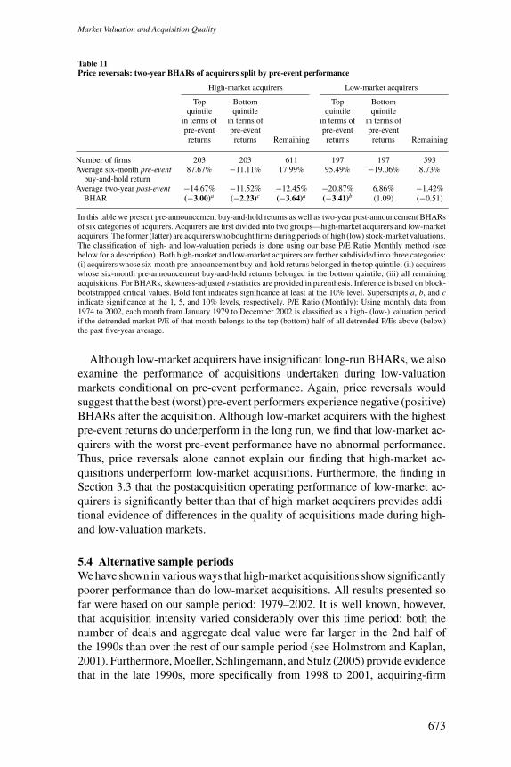
Market Valuation and Acquisition Quality
Table 11Price reversals: two-year BHARs of acquirers split by pre-event performance
High-market acquirers Low-market acquirers
Top Bottom Top Bottomquintile quintile quintile quintile
in terms of in terms of in terms of in terms ofpre-event pre-event pre-event pre-eventreturns returns Remaining returns returns Remaining
Number of firms 203 203 611 197 197 593Average six-month pre-event 87.67% −11.11% 17.99% 95.49% −19.06% 8.73%
buy-and-hold returnAverage two-year post-event −14.67% −11.52% −12.45% −20.87% 6.86% −1.42%
BHAR (−3.00)a (−2.23)c (−3.64)a (−3.41)b (1.09) (−0.51)
In this table we present pre-announcement buy-and-hold returns as well as two-year post-announcement BHARsof six categories of acquirers. Acquirers are first divided into two groups—high-market acquirers and low-marketacquirers. The former (latter) are acquirers who bought firms during periods of high (low) stock-market valuations.The classification of high- and low-valuation periods is done using our base P/E Ratio Monthly method (seebelow for a description). Both high-market and low-market acquirers are further subdivided into three categories:(i) acquirers whose six-month pre-announcement buy-and-hold returns belonged in the top quintile; (ii) acquirerswhose six-month pre-announcement buy-and-hold returns belonged in the bottom quintile; (iii) all remainingacquisitions. For BHARs, skewness-adjusted t-statistics are provided in parenthesis. Inference is based on block-bootstrapped critical values. Bold font indicates significance at least at the 10% level. Superscripts a, b, and cindicate significance at the 1, 5, and 10% levels, respectively. P/E Ratio (Monthly): Using monthly data from1974 to 2002, each month from January 1979 to December 2002 is classified as a high- (low-) valuation periodif the detrended market P/E of that month belongs to the top (bottom) half of all detrended P/Es above (below)the past five-year average.
Although low-market acquirers have insignificant long-run BHARs, we alsoexamine the performance of acquisitions undertaken during low-valuationmarkets conditional on pre-event performance. Again, price reversals wouldsuggest that the best (worst) pre-event performers experience negative (positive)BHARs after the acquisition. Although low-market acquirers with the highestpre-event returns do underperform in the long run, we find that low-market ac-quirers with the worst pre-event performance have no abnormal performance.Thus, price reversals alone cannot explain our finding that high-market ac-quisitions underperform low-market acquisitions. Furthermore, the finding inSection 3.3 that the postacquisition operating performance of low-market ac-quirers is significantly better than that of high-market acquirers provides addi-tional evidence of differences in the quality of acquisitions made during high-and low-valuation markets.
5.4 Alternative sample periodsWe have shown in various ways that high-market acquisitions show significantlypoorer performance than do low-market acquisitions. All results presented sofar were based on our sample period: 1979–2002. It is well known, however,that acquisition intensity varied considerably over this time period: both thenumber of deals and aggregate deal value were far larger in the 2nd half ofthe 1990s than over the rest of our sample period (see Holmstrom and Kaplan,2001). Furthermore, Moeller, Schlingemann, and Stulz (2005) provide evidencethat in the late 1990s, more specifically from 1998 to 2001, acquiring-firm
673

The Review of Financial Studies / v 22 n 2 2009
Table 12Alternative sample periods: difference in two-year BHARs for high- and low-market acquisitions
Full sample 1979–1994 versus 1995–2002 1979–1997 versus 1998–2002
1979–2002 1979-1994 1995–2002 1979–1997 1998–2002
High-market minus low-market −8.04% −8.97% −8.47% −15.82% −12.83%(2.60)a (−1.31) (−2.49)a (−2.60)a (−2.97)a
Cash acquisitions minus −12.64% −7.41% −13.04% −6.35% −17.57%stock acquisitions (−4.47)a (−1.59) (−3.84)a (−1.68)c (−4.30)a
High-market cash minus −14.76% 1.61% −18.23% −10.52% −20.08%low-market cash (−3.09)a (0.18) (−3.41)a (−1.34) (−3.14)a
High-market stock minus −4.93% −32.9% −2.30% −30.73% −6.07%low-market stock (−0.95) (−2.29)b (−0.41) (−2.48)a (−0.83)
Tender offers minus mergers 10.15% 14.40% 2.78% 14.72% 1.05%(2.75)a (2.37)a (0.62) (2.91)a (0.20)
High-market tenders minus −3.80% 16.54% −12.61 7.43% −31.61%low-market tenders (−0.49) (1.25) (−1.39) (0.65) (−3.18)a
High-market mergers minus −8.54% −17.68% −7.96% −21.16% −11.01%low-market mergers (−2.54)a (−2.19)b (−2.18)b (−2.91)a (−2.35)a
This table presents the difference between the two-year BHARs of acquisitions undertaken during high- andlow-valuation periods for five alternative sample periods: 1979–1994, 1995–2002, 1979–1997, 1998–2002, and1979–2002. The classification of high- and low-valuation periods is done using our base P/E Ratio (Monthly)method: each month is classified as a high- (low-) valuation market if the detrended market P/E of that monthbelongs to the top (bottom) half of all detrended P/Es above (below) the past five-year average. t-statistics areprovided in parenthesis. Bold font indicates significance at least at the 10% level. Superscripts a, b, and c indicatesignificance at the 1, 5, and 10% levels, respectively. Significance is based on block-bootstrapped critical values.
shareholders experienced massive losses around the acquisition announcementdate that dwarfed losses experienced in the 1980s and early 1990s. Given thesefindings, could it be that our results are driven by acquisitions announced inthe 2nd half of the 1990s or the late 1990s? To investigate this possibility, wesplit our sample period into acquisitions announced from 1979 to 1994 versus1995 to 2002, and acquisitions announced from 1979 to 1997 versus 1998 to2002. We rerun our tests using BHARs.27
Table 12 shows that high-market acquisitions underperform low-market ac-quisitions over all time periods considered. (The difference is significant for allperiods except 1979–1994.) The underperformance seems to be driven by merg-ers: high-market mergers show significantly lower BHARs than do low-marketmergers over all periods. Although the performance of high- and low-marketacquisitions is not significantly different in the 1979–1994 period, it is note-worthy that almost 80% of deals announced during this period were mergers:as is evident in Table 12, high-market mergers significantly underperformedlow-market mergers in the 1979–1994 period.
Some differences do exist among time periods. First, stock acquisitionsunderperform cash acquisitions, but the difference is not significant over theearlier period (1979–1994). Second, high-market cash deals significantly under-perform over the later periods (1995–2002 and 1998–2002), while high-market
27 Sample sizes are too small to run tests in calendar time. For example, while there were 463 low- and 884 high-market acquisitions from 1998 to 2002, those deals were announced over a mere 17 high- and 36 low-valuationmarkets.
674

Market Valuation and Acquisition Quality
stock deals significantly underperform over the earlier periods (1979–1994and 1979–1997). Third, tender offers outperform mergers, but the differenceis only significant over the earlier time periods (1979–1994 and 1979–1997).And, fourth, high-market tenders underperform low-market tenders, but thedifference is only significant for the late 1990s (1998–2002).
In sum, differences do exist for deals announced over the different timeperiods. However, key is that the underperformance of high-market acquisitionsdoes not seem to be driven by the 2nd half of the 1990s or the late 1990s.
6. Conclusion
Motivated by the recent theoretical models that explain how stock market levelsmay influence managerial acquisition decisions and acquisition quality, we askthe following: Are acquisitions that are announced when the market is boomingfundamentally different from those that are initiated during market troughs?
We conclude they are. We examine the stock and operating performanceof acquisitions initiated when markets are booming (high-valuation markets)and when they are depressed (low-valuation markets), and find that marketvaluations at the time acquisitions are initiated are correlated with acquirer per-formance in a way that is consistent with the theories. Although announcementreturns are significantly better for acquisitions announced in high-valuationmarkets relative to those announced in low-valuation markets, this finding isreversed in the long run. Consistent with existing theory, acquirers buying inhigh-valuation markets significantly underperform relative to acquirers buyingduring low-valuation markets in the two years following the acquisition. Theseresults hold in a univariate setting and in a multivariate regression framework inwhich we control for various other factors that may affect acquirer performance,including method of payment, the type of acquisition (tender/merger), and theacquirer’s own M/B. Furthermore, these findings are robust to the methodologyused to classify high- and low-valuation markets and the measure of abnormalperformance used (BHARs, calendar-time portfolio returns, or acquirer operat-ing performance). Finally, we demonstrate that the reversal of fortunes for theacquirers is not simply a manifestation of short-term persistence and long-termreversals.
Our overall conclusion that acquirer performance is correlated with the stateof the market is consistent with recent evidence that stock prices affect corporatedecisions. Our results strongly suggest that, viewed through an ex post perfor-mance lens, acquisitions undertaken during periods of high-market valuationsare of lower quality than those undertaken during periods of low-market valua-tions. We find that the underperformance of acquirers buying in high-valuationmarkets cannot be explained by overpayment, and does not seem consistentwith market timing. However, our results are consistent with herding behaviorby managers: underperformance of acquisitions undertaken when markets arebooming is caused by firms that buy later in the merger wave.
675

The Review of Financial Studies / v 22 n 2 2009
Appendix A: Creation of Reference Portfolios
To create the reference portfolios, we calculate 50 size and book-to-marketportfolios in the spirit of Fama and French (1993). Following Loughran andRitter (2000), we do not include firms in our reference portfolios that didan acquisition during the year the portfolio was created or during the fourpreceding years, since inclusion of such firms would bias our tests towardfinding no abnormal returns.
The size and book-to-market portfolios are created in two steps followingFama and French (1993). First, in June of each year t from 1978 to 2001, werank all NYSE firms on CRSP on the basis of their market value of equity.The market value of equity is calculated using the price and common sharesoutstanding as of end June. Size deciles are then created on the basis of theserankings for all NYSE firms. Second, within each size decile, firms are sortedinto quintiles based on their book-to-market ratios in year t − 1.28 Book valueof equity is defined as the Compustat book value of stockholder’s equity, plusbalance sheet deferred taxes and investment tax credit, minus the book valueof preferred stock. As in Fama and French (1993) we use the redemption,liquidation, or par value (in that order) to estimate the value of preferred stock.The book-to-market ratio in year t − 1 is calculated as the book value of equityfor fiscal year ending in calendar year t − 1, divided by market equity at the endof December of year t − 1. We drop firms that have negative book-to-marketratios when calculating book-to-market breakpoints.
Once NYSE firms have been ranked as above, NASDAQ and AMEX firmsare placed in the appropriate size/book-to-market portfolio based on their sizein June of year t and their book-to-market ratio in year t − 1.
Appendix B: Testing for Significance in Our BHAR Analysis
Lyon, Barber, and Tsai (1999) argue that since BHARs are positively skewed,inference should not be based on the normality assumption. Instead, one mustuse the skewness-adjusted test statistic and bootstrap the critical values in orderto draw inference. The skewness-adjusted t-statistic is as follows:
t = √n
(S + 1
3γS2 + 1
6nγ
), (B1)
where
S = BHAR
σ(BHAR)and γ =
∑ni=1 (BHARi − BHAR)3
nσ(BHAR)3(B2)
In the equations above, γ is an estimate of the coefficient of skewness, nis the sample size, and
√nS is the conventional t-statistic. We follow this
28 The time at which the market value of equity and book-to-market are calculated for ranking purposes is basedon Fama and French (1993) and Barber and Lyon (1997).
676

Market Valuation and Acquisition Quality
methodology albeit with one important distinction. Bootstrap sampling mustbe carried out in a way that suitably captures the dependence structure of theoriginal sample. Independent sampling assumes that abnormal returns of eventfirms are independent. As argued by Mitchell and Stafford (2000), major cor-porate actions are not independent events, and thus event samples are unlikelyto consist of independent observations. To preserve the dependence structure ofthe original data we create bootstrap samples via the block bootstrap procedureoutlined in Horowitz (2003). In the block bootstrap procedure, the original dataare divided into blocks. The bootstrap sample is obtained by sampling overlap-ping blocks randomly with replacement and laying them end-to-end in the ordersampled. The sampling of the blocks must be such that the block-bootstrappedsample is at least of length n, where n is the length of the original data. We draw2000 bootstrapped samples in this manner and calculate the critical values.29
Note that since we bootstrap these critical values, their values do not corre-spond to the critical values from the normal distribution. This explains why,e.g., in Table 3, the performance of mixed payment tender offers is significanteven though the t-statistic is 1.01 (see panel A), and why the performance oflow-market stock acquirers is not significant even though the t-statistic is 1.89(see panel D).
ReferencesAgrawal, A., J. F. Jaffe, and G. N. Mandelker. 1992. The Post-Merger Performance of Acquiring Firms: ARe-Examination of an Anomaly. Journal of Finance 47:1605–21.
Andrade, G., M. Mitchell, and E. Stafford. 2001. New Evidence and Perspectives on Mergers. Journal ofEconomic Perspectives 15:103–20.
Ang, J., and Y. Cheng. 2006. Direct Evidence on the Market-Driven Acquisitions Theory. Journal of FinancialResearch 29:199–216.
Asquith, P., R. F. Bruner, and D. W. Mullins. 1983. The Gains to Bidding Firms from Merger. Journal of FinancialEconomics 11:121–39.
Banerjee, A. V. 1992. A Simple Model of Herd Behavior. Quarterly Journal of Economics 107:797–817.
Barber, B. M., and J. D. Lyon. 1996. Detecting Abnormal Operating Performance: The Empirical Power andSpecification of Test Statistics. Journal of Financial Economics 41:359–99.
Barber, B. M., and J. D. Lyon. 1997. Detecting Long-Run Abnormal Stock Returns: The Empirical Power andSpecification of Test Statistics. Journal of Financial Economics 43:341–72.
Bikhchandani, S., D. Hirshleifer, and I. Welch. 1998. Learning from the Behavior of Others: Conformity, Fads,and Informational Cascades. Journal of Economic Perspectives 12:151–70.
Bradley, M., A. Desai, and E. H. Kim. 1988. Synergistic Gains from Corporate Acquisitions and Their DivisionBetween the Stockholders of Target and Acquiring Firms. Journal of Financial Economics 21:3–40.
Brown, S., and J. Warner. 1985. Using Daily Stock Returns: The Case of Event Studies. Journal of FinancialEconomics 14:3–31.
Bruner, R. F. 2002. Does M&A Pay? A Survey of Evidence for the Decision-Maker. Journal of Applied Finance12:48–68.
29 We choose a block size equal to n/10 where n is the length of the original data. The bootstrapped critical valuesdo not change significantly for small changes in the block size.
677

The Review of Financial Studies / v 22 n 2 2009
Carhart, M. 1997. On Persistence in Mutual Fund Performance. Journal of Finance 52:57–82.
Dennis, D. K., and J. J. McConnell. 1986. Corporate Mergers and Security Returns. Journal of FinancialEconomics 16:143–87.
Dong, M., D. Hirshleifer, S. Richardson, and S. H. Teoh. 2006. Does Investor Misvaluation Drive the TakeoverMarket? Journal of Finance 61:725–62.
Eckbo, B. E., R. M. Giammarino, and R. L. Heinkel. 1990. Asymmetric Information and the Medium of Exchangein Takeovers: Theory and Tests. Review of Financial Studies 3:651–75.
Fama, E. F., and K. R. French. 1993. Common Risk Factors in the Returns on Stocks and Bonds. Journal ofFinancial Economics 33:3–56.
Franks, J., R. Harris, and S. Titman. 1991. The Postmerger Share-Price Performance of Acquiring Firms. Journalof Financial Economics 29:81–96.
Fuller, K., J. Netter, and M. Stegemoller. 2002. What Do Returns to Acquiring Firms Tell Us? Evidence fromFirms that Make Many Acquisitions. Journal of Finance 57:1763–93.
Goel, A., and A. V. Thakor. 2005. Envy and Merger Waves. Working Paper, DePaul University and WashingtonUniversity in St. Louis.
Hansen, R. G., and J. R. Lott. 1996. Externalities and Corporate Objectives in a World with Diversified Share-holders/Consumers. Journal of Financial and Quantitative Analysis 31:43–68.
Harford, J. 1999. Corporate Cash Reserves and Acquisitions. Journal of Finance 54:1969–97.
Harford, J. 2005. What Drives Merger Waves? Journal of Financial Economics 77:529–60.
Healy, P., K. Palepu, and R. Ruback. 1992. Does Corporate Performance Improve after Mergers? Journal ofFinancial Economics 31:135–75.
Heron, R., and E. Lie. 2002. Operating Performance and the Method of Payment in Takeovers. Journal ofFinancial and Quantitative Analysis 37:137–55.
Holmstrom, B., and S. Kaplan. 2001. Corporate Governance and Merger Activity in the United States: MakingSense of the 1980s and 1990s. Journal of Economic Perspectives 15:121–44.
Horowitz, J. L. 2003. The Bootstrap in Econometrics. Statistical Science 29:199–216.
Jegadeesh, N., and S. Titman. 1993. Returns to Buying Winners and Selling Losers: Implications for StockMarket Efficiency. Journal of Finance 48:65–91.
Jensen, M. C., and R. S. Ruback. 1983. The Market for Corporate Control: The Scientific Evidence. Journal ofFinancial Economics 11:5–50.
Jovanovic, B., and P. Rousseau. 2001. Mergers and Technological Change: 1885–1998. Working Paper 01-W16,Vanderbilt University.
Jovanovic, B., and S. Braguinsky. 2004. Bidder Discounts and Target Premia in Takeovers. American EconomicReview 94:46–56.
Loughran, T., and J. R. Ritter. 1997. The Operating Performance of Firms Conducting Seasoned Equity Offerings.Journal of Finance 52:1823–50.
Loughran, T., and J. R. Ritter. 2000. Uniformly Least Powerful Tests of Market Efficiency. Journal of FinancialEconomics 55:361–89.
Loughran, T., and A. M. Vijh. 1997. Do Long-Term Shareholders Benefit from Corporate Acquisitions? Journalof Finance 52:1765–90.
Lyon, J. D., B. M. Barber, and C. Tsai. 1999. Improved Methods for Tests of Long-Run Abnormal Stock Returns.Journal of Finance 54:165–201.
678

Market Valuation and Acquisition Quality
Mitchell, M. L., and J. H. Mulherin. 1996. The Impact of Industry Shocks on Takeover and Restructuring Activity.Journal of Financial Economics 41:193–229.
Mitchell, M. L., and E. Stafford. 2000. Managerial Decisions and Long-Term Stock Price Performance. Journalof Business 73:287–329.
Moeller, S. B., F. P. Schlingemann, and R. M. Stulz. 2004. Firm Size and the Gains from Acquisitions. Journalof Financial Economics 73:201–28.
Moeller, S. B., F. P. Schlingemann, and R. M. Stulz. 2005. Wealth Destruction on a Massive Scale? A Study ofAcquiring-Firm Returns in the Recent Merger Wave. Journal of Finance 60:757–82.
Nelson, R. L. 1959. Merger Movements in American Industry, 1895–1956. Princeton, NJ: Princeton UniversityPress.
Persons, J. C., and V. Warther. 1997. Boom and Bust Patterns in the Adoption of Financial Innovations. Reviewof Financial Studies 10:939–67.
Rau, P. R., and T. Vermaelen. 1998. Glamour, Value, and the Postacquisition Performance of Acquiring Firms.Journal of Financial Economics 49:223–53.
Rhodes-Kropf, M., D. T. Robinson, and S. Viswanathan. 2005. Valuation Waves and Merger Activity: TheEmpirical Evidence. Journal of Financial Economics 77:561–603.
Rhodes-Kropf, M., and S. Viswanathan. 2004. Market Valuation and Merger Waves. Journal of Finance 59:2685–718.
Schwert, G. W. 2000. Hostility in Takeovers: In the Eyes of the Beholder? Journal of Finance 55:2599–640.
Shleifer, A., and R. W. Vishny. 2003. Stock Market Driven Acquisitions. Journal of Financial Economics70:295–311.
679