Equity Valuation Using Multiples: An Empirical Investigation

DISSERTATION of the University of St.Gallen

Graduate School of Business Administration, Economics, Law and Social Sciences (HSG)

to obtain the title of Doctor of Business Administration

submitted by Andreas Schreiner

from Austria

Approved on the application of Prof. Dr. Klaus Spremann

and Prof. Dr. Thomas Berndt

Dissertation no. 3313 Deutscher Universitäts-Verlag, Wiesbaden 2007

The University of St. Gallen, Graduate School of Business Administration, Eco-nomics, Law and Social Sciences (HSG) hereby consents to the printing of the pre-sent dissertation, without hereby expressing any opinion on the views herein ex-pressed. St. Gallen, January 22, 2007 The President:

Prof. Ernst Mohr, Ph.D.

Foreword

Accounting-based market multiples are the most common technique in equity valuation. Multiples are used in research reports and stock recommendations of both buy-side and sell-side analysts, in fairness opinions and pitch books of investment bankers, or at road shows of firms seeking an IPO. Even in cases where the value of a corporation is primarily determined with discounted cash flow, multiples such as P/E or market-to-book play the important role of providing a second opinion. Mul-tiples thus form an important basis of investment and transaction decisions of vari-ous types of investors including corporate executives, hedge funds, institutional in-vestors, private equity firms, and also private investors.

In spite of their prevalent usage in practice, not so much theoretical back-ground is provided to guide the practical application of multiples. The literature on corporate valuation gives only sparse evidence on how to apply multiples or on why individual multiples or comparable firms should be selected in a particular context.

The present book by Andreas Schreiner develops a comprehensive multiples valuation framework, which overcomes many of these problems. It gives answers to many questions, which have not been clarified so far, and which must be addressed in order to come up with sound and convincing valuations in practice. After an in-troduction and a review of the literature, Schreiner outlines the theoretical founda-tions of equity valuation using multiples. He derives intrinsic multiples from fun-damental equity valuation models and explains why some firms deserve higher or lower multiples than its peers. Based on the weaknesses of the standard multiples valuation method, Schreiner systematically develops a list of criteria for the selec-tion of relevant multiples and the identification of comparable firms. The introduc-tion of an adjustment factor in the valuation equation offers a solution to the ques-tion, how to account for strategic advantages of the firm being valued over the peer group. Then, a two-factor multiples model is presented to combine information pro-vided by two different multiples into a single valuation equation.

The book enriches the research on multiples with an extensive empirical study of European and U.S. equity markets. The results of the study, which exhibit high significance and robustness, approve the relevance of the multiples valuation

IV Foreword framework. Schreiner demonstrates quite a number of results such as (1) the use of market capitalization as market price variable in the numerator of a multiple; (2) the consideration of knowledge-related variables in science-based industries; (3) the incorporation of forward-looking information; and (4) the usage of a preferably fine industry definition. For a selection of five key industries, Schreiner finds empirical support for the existence of industry-preferred multiples when using trailing multi-ples and for the usefulness of the two-factor model.

With his work, Andreas Schreiner makes an influential contribution to the the-ory and practice of corporate valuation using multiples. The straightforwardness of the underlying framework and the empirical results make the book an important reference for practitioners. I recommend this book to professionals in corporate fi-nance and equity research, and wish that it wins the broad readership it deserves.

Dr. Klaus SpremannProfessor and Director

Swiss Institute of Banking and Finance

Preface

Reviewing my time as a research associate makes me feel as if a dream had turned into reality. This dream combined unique learning experiences on both an academic and a personal level with full enjoyment and diversity of life. Within the dream, there have been many people, whom I want to thank for helping me in one way or the other during the last three years. Foremost my deepest gratitude goes to Professor Klaus Spremann, my advisor and academic teacher. He gave me the re-quired inspiration and guidance to explore my potentials and utilize them in this book. My working experience with him as an assistant and as a research associate at the Swiss Institute of Banking and Finance at the University of St.Gallen exceeded all my expectations: he taught me the economics of corporate finance and portfolio management in his books and seminars as well as in our conversations and meet-ings. I learned from him to approach challenging tasks with the right attitude and experienced what it means to grow with confidence and responsibility.

Profound gratitude also goes to Professor Thomas Berndt, who spontaneously agreed to supervise my work as a co-adviser. His enthusiasm and thoughts sparked my interest in many areas of accounting and made him a great mentor. Likewise, I am very grateful to Professor Pascal Gantenbein. He initiated my passion for the world of finance when I arrived as a master student at the University of St.Gallen in 2004, and since then advised, encouraged, and supported me at any time in various aspects of life.

Within the twelve-month period as a visiting researcher at the Anderson School of Management at UCLA and the Yale School of Management in 2006/2007, the quality and substance of my research gained enormously from the faculty input I received from Professor Jing Liu, Professor David Aboody (both UCLA), and Professor Jacob Thomas (Yale). Special thanks also goes to Dean Al Osborne, Dean Eric Mokover (both UCLA), and Professor Subrata Sen (Yale) for making this unforgettable experience possible. Financial support for this research visit by the Swiss National Science Foundation is gratefully acknowledged.

Changing environments and the speed of life pose a challenge for friendships and relationships. Notwithstanding, I enjoyed grand benevolence and encourage-

VI Preface ment from my friends, which I deeply appreciate. Sebastian Lang, Jan Bernhard, Andreas Zingg, and several other colleagues at the Swiss Institute of Banking and Finance were always available to share thoughts and provide feedback. My work also benefited from conversations with students of the Doctoral and the MAccFin program at the University of St.Gallen, in particular with John von Berenberg-Consbruch, whom I supervised with his master thesis. Similarly, I received helpful comments from Ph.D. students at the finance department at UCLA, notably Yuzhao Zhang, and Ph.D. students at the School of Management at Yale, notably Panagiotis Patatoukas.

Philipp Hirzberger, Ralph Huber, Phillip Kirst, Kay Oppat, Martin Pansy, and many other friends supported me by providing the necessary mental balance at all times in Switzerland and back home in Austria. Toni Schmidt, Tobias Baumann, András Kadocsa, Tim Malonn, and Saskia Pfauter in Los Angeles as well as Tatiana Alekseeva and Christoph Lassenberger in New Haven, together with many friends visiting me from Europe, in particular Michael Pucher and Kerstin Stockinger, joined me to explore the beauties and leisure opportunities of the American East and West Coast. Mike Finley carefully proofread the manuscript on grammar and style issues. However, all remaining deficiencies and errors are mine.

Finally, I thank my parents Johannes and Renate Schreiner, together with my sister Julia. Their love and patience is what I always rely on. St. Gallen, January 22, 2007 Andreas Schreiner

Executive summary

This book is motivated by the apparent gap between the widespread usage of multiples in valuation practice and the deficiency of relevant research related to multiples. While valuing firms using multiples seems straightforward on the sur-face, it actually invokes several complications and open issues. To close this gap, the book examines the role of multiples in equity valuation and transforms the stan-dard multiples valuation method into a comprehensive framework for using multi-ples in equity valuation.

To identify the underlying drivers of different multiples, I derive intrinsic mul-tiples from fundamental equity valuation models. An overview of common market multiples and the standard multiples valuation method including its criticism initi-ates an in-depth analysis of every single step of the four-step multiples valuation process. I investigate key criteria for the selection of value relevant measures and for the identification of comparable firms, and assess the usefulness of a two-factor multiples valuation model combining book value and earnings multiples from a theoretical point of view.

In the empirical study, I find that multiples generally approximate market val-ues reasonably well. In terms of relative performance, the results show that: (1) eq-uity value multiples outperform entity value multiples; (2) knowledge-related mul-tiples outperform traditional multiples in science-based industries; and (3) forward-looking multiples, in particular the two-year forward-looking P/E multiple, outper-form trailing multiples. For the selection of comparable firms, the results suggest the use of a preferably fine industry definition. While I find support for the general perception that different industries are associated with different best multiples among trailing multiples, including forecast material reveals a clear dominance of the two-year forward-looking P/E multiple across industries. The results of the analysis of the properties and valuation accuracy of the two-factor multiples valua-tion model provide evidence for the theoretical reasoning that the usefulness of in-corporating the P/B multiple as a second decision relevant multiple into the two-factor model depends on: (1) its valuation accuracy in a specific industry; and (2) the exclusiveness of information provided over the first decision relevant multiple.

Brief contents

1 Introduction .....................................................................................................1

1.1 Motivation.................................................................................................1

1.2 Research idea ............................................................................................5

1.3 Outline of the book .................................................................................11

2 Literature review ...........................................................................................13

2.1 Coverage in standard literature ...............................................................13

2.2 Empirical research ..................................................................................15

2.3 Contribution to prior research.................................................................20

3 Theoretical foundations ................................................................................22

3.1 Theoretical concept of fundamental equity valuation models................22

3.2 Derivation of intrinsic multiples.............................................................31

3.3 Market multiples .....................................................................................38

4 Comprehensive multiples valuation.............................................................48

4.1 The standard multiples valuation method and its criticism ....................48

4.2 Selection of value relevant measures......................................................56

4.3 Identification of comparable firms .........................................................68

4.4 Estimation of synthetic peer group multiples .........................................74

4.5 Actual valuation......................................................................................76

4.6 Two-factor multiples valuation model....................................................80

5 Design of the empirical study .......................................................................84

5.1 The concept of value relevance ..............................................................84

5.2 Research hypotheses ...............................................................................88

5.3 Research methodology............................................................................89

5.4 Data and sample......................................................................................93

Brief contents IX

6 Empirical results ........................................................................................... 98

6.1 Cross-sectional analysis ......................................................................... 98

6.2 Industry analysis................................................................................... 113

6.3 Evaluation of empirical results............................................................. 121

7 Conclusion.................................................................................................... 127

7.1 Summary of findings ............................................................................ 127

7.2 Implications for practice....................................................................... 129

7.3 Research outlook .................................................................................. 130

Contents

Foreword............................................................................................................ III

Preface.................................................................................................................. V

Executive summary..........................................................................................VII

Brief contents.................................................................................................. VIII

Contents ............................................................................................................... X

List of figures...................................................................................................XIV

List of tables...................................................................................................... XV

Notations and abbreviations ..........................................................................XVI

1 Introduction .....................................................................................................1

1.1 Motivation.................................................................................................1

1.2 Research idea ............................................................................................5

1.2.1 Research questions for the theoretical part ..................................5

1.2.2 Research questions for the empirical part....................................7

1.2.3 Research design of the empirical study .....................................10

1.3 Outline of the book .................................................................................11

2 Literature review ...........................................................................................13

2.1 Coverage in standard literature ...............................................................13

2.2 Empirical research ..................................................................................15

2.2.1 Valuation accuracy of the multiples valuation method .............15

2.2.2 Selection of value relevant measures.........................................16

2.2.3 Identification of comparable firms.............................................17

2.2.4 Industry-preferred multiples ......................................................19

2.2.5 Combination of multiples ..........................................................19

2.3 Contribution to prior research.................................................................20

Contents XI

3 Theoretical foundations ................................................................................ 22

3.1 Theoretical concept of fundamental equity valuation models ............... 22

3.1.1 Dividend discount model........................................................... 23

3.1.2 Discounted cash flow model...................................................... 24

3.1.3 Residual income valuation model ............................................. 27

3.1.4 Abnormal earnings growth model ............................................. 29

3.2 Derivation of intrinsic multiples............................................................. 31

3.2.1 Intrinsic P/E multiple derived from the DDM........................... 32

3.2.2 Intrinsic EV/EBIT multiple derived from the DCF model........ 33

3.2.3 Intrinsic P/B multiple derived from the RIV model.................. 35

3.3 Market multiples..................................................................................... 38

3.3.1 Definition and categorization of market multiples.................... 38

3.3.2 Common equity value and entity value multiples ..................... 41

3.3.3 Alternative multiples ................................................................. 43

3.3.4 Trailing and forward-looking multiples .................................... 47

4 Comprehensive multiples valuation ............................................................ 48

4.1 The standard multiples valuation method and its criticism.................... 48

4.1.1 Concept of the multiples valuation method............................... 48

4.1.2 Four step valuation process ....................................................... 49

4.1.3 Strengths and weaknesses of the standard multiples method.... 53

4.2 Selection of value relevant measures ..................................................... 56

4.2.1 Equity value versus entity value multiples................................ 57

4.2.2 Industry specific multiples......................................................... 62

4.2.3 Time reference of value drivers................................................. 65

4.2.4 Criteria for the selection of value relevant measures ................ 66

4.3 Identification of comparable firms ......................................................... 68

4.3.1 Industry classification systems .................................................. 69

4.3.2 Assessment of comparability..................................................... 70

4.3.3 Size of the peer group................................................................ 72

4.3.4 Criteria for the identification of comparable firms.................... 73

4.4 Estimation of synthetic peer group multiples......................................... 74

XII Contents

4.5 Actual valuation......................................................................................76

4.5.1 Ratio analysis .............................................................................76

4.5.2 Adjustment factor.......................................................................78

4.6 Two-factor multiples valuation model....................................................80

4.6.1 Decision relevant multiples and hedging multiples...................80

4.6.2 Combination of two decision relevant multiples .......................81

5 Design of the empirical study .......................................................................84

5.1 The concept of value relevance ..............................................................84

5.1.1 Definition, interpretation, implementation ................................84

5.1.2 The link between value relevance and market efficiency..........86

5.2 Research hypotheses ...............................................................................88

5.3 Research methodology............................................................................89

5.3.1 Methodology using single multiples..........................................90

5.3.2 Methodology using combined multiples....................................92

5.4 Data and sample......................................................................................93

6 Empirical results............................................................................................98

6.1 Cross-sectional analysis..........................................................................98

6.1.1 Absolute valuation accuracy ......................................................98

6.1.2 Equity value versus entity value multiples ..............................101

6.1.3 Knowledge-related versus traditional multiples ......................104

6.1.4 Forward-looking versus trailing multiples...............................106

6.1.5 The effect of industry fineness.................................................110

6.2 Industry analysis ...................................................................................113

6.2.1 Industry-preferred multiples ....................................................114

6.2.2 Single versus combined multiples ...........................................117

6.3 Evaluation of empirical results .............................................................121

6.3.1 Validation using U.S. data .......................................................121

6.3.2 Limitations ...............................................................................124

Contents XIII

7 Conclusion.................................................................................................... 127

7.1 Summary of findings ............................................................................ 127

7.2 Implications for practice....................................................................... 129

7.3 Research outlook .................................................................................. 130

Appendix A: ICB industry classification structure...................................... 131

Appendix B: U.S. evidence.............................................................................. 135

Appendix C: Definition of variables .............................................................. 151

References......................................................................................................... 154

List of figures1

Figure 1.1: Valuation models employed in analysts’ reports ..............................2

Figure 1.2: Outline of the book..........................................................................12

Figure 3.1: Intrinsic multiples derived from fundamental valuation models ....38

Figure 3.2: Categorization of multiples .............................................................39

Figure 4.1: Open issues of the standard multiples method................................53

Figure 4.2: Strengths and weaknesses of the standard multiples method..........56

Figure 4.3: List of criteria for the selection of value relevant measures ...........68

Figure 4.4: List of criteria for the identification of comparable firms...............74

Figure 6.1: Performance of equity value versus entity value multiples ..........103

Figure 6.2: Performance of forward-looking versus trailing multiples ...........109

Figure 6.3: Performance of multiples depending on the industry fineness .....112

Figure 6.4: Time stability of calibrated absolute valuation errors in Europe ..125

1 List excludes figures in the Appendices.

List of tables2

Table 5.1: Sample characteristics and descriptive statistics.............................. 95

Table 5.2: Equity value multiples summary statistics ....................................... 97

Table 6.1: Absolute valuation accuracy of equity value multiples ................. 100

Table 6.2: Performance of equity value versus entity value multiples ........... 102

Table 6.3: Performance of knowledge-related versus traditional multiples.... 106

Table 6.4: Performance of forward-looking versus trailing multiples ............ 108

Table 6.5: Performance of multiples depending on the industry fineness ...... 111

Table 6.6: Dow Jones STOXX 600 industry weights ..................................... 113

Table 6.7: Industry-preferred multiples in European key industries............... 115

Table 6.8: Correlations among selected value drivers .................................... 118

Table 6.9: Factors and weights of the two-factor multiples valuation model in European key industries ............................................................. 119

Table 6.10: Performance of single versus combined multiples in selected European key industries ................................................................. 121

Table 6.11: Comparison of absolute valuation accuracy in European and U.S. equity markets ........................................................................ 122

2 List excludes tables in the Appendices.

Notations and abbreviations

Price and value

net debtb Book value of net debt equityp Stock price / market value of common equity entityp Market value of common equity plus book value of net debt

net debtp Market value of net debt equityv Equity value / intrinsic value of common equity entityv Entity value / intrinsic value of common equity plus net debt

Variables used to construct multiples3

AIA Amortization of intangible assets B Book value of common equity D (Ordinary cash) dividend E Earnings EBIT Earnings before interest and taxes EBITDA Earnings before interest, taxes, depreciation, and amortization EBT Earnings before taxes / pre-tax income EV Enterprise value (equivalent to entityp )

GI Gross income IC Invested capital KC Knowledge costs R&D R&D expenditures OCF Operating cash flow / cash flow from operating activities P (Stock) price / market capitalization (equivalent to equityp )

SA Sales / revenues TA Total assets

3 For more details, see Appendix C.

Notations and abbreviations XVII

Additional abbreviations

AE Abnormal earnings AEG Abnormal earnings growth CAPEX Capital expenditures CAPM Capital asset pricing model ch. Chapter / -s DCF Discounted cash flow / -s DDM Dividend discount model DS Datastream e.g. Exempli gratia (for example) EMH Efficient market hypothesis EPS Earnings per share et al. Et alii (and others) EU European Union EVA Economic Value Added FASB Financial Accounting Standards Board FCF Free cash flow / -s FFIG Fama and French industry groupings FTSE Financial Times Stock Exchange GAAP Generally Accepted Accounting Principles GGM Gordon growth model GICS Global Industry Classification Standards HSG University of St.Gallen I/B/E/S Institutional Brokers Estimate Service i.e. Id est (that is) IAS International Accounting Standards IASB International Accounting Standards Board ICB Industry Classification Benchmark IFRS International Financial Reporting Standards IPO Initial public offering ISIC International Standard Industrial Classification LBO Leveraged buyout

XVIII Notations and abbreviations M&A Mergers & acquisitions MBA Master of business administration MBO Management buyout MIT Massachusetts Institute of Technology MP Multiples / -s MSCI Morgan Stanley Capital International n Number of observations NAICS North American Industry Classification System NI Net income available to common shareholders (equivalent to E) NZZ Neue Zürcher Zeitung p. Page / -s PEG Price to earnings to earnings growth PR (Dividend) payout ratio R&D Research & development RI Residual income (equivalent to AE) RIV Residual income valuation ROA Return on assets ROCE Return on common equity ROIC Return on invested capital $ U.S. Dollar S&P Standard and Poor’s SEC Securities and Exchange Commission SFAS Statement of Financial Accounting Standards SIC Standard Industrial Classification SWOT Strengths, weaknesses, opportunities, and threats T Tax rate UCLA University of California at Los Angeles U.S. United States

equityr Cost of equity waccr Weighted average cost of capital

WC Worldscope

1 Introduction

1.1 Motivation

Equity valuation is a primary application of finance and accounting theory. A typical business school curriculum, therefore, devotes substantial time to this topic. The theoretical emphasis usually focuses on discounted cash flow (DCF) and resid-ual income valuation (RIV) models. These models, however, are often cumbersome to use and sensitive to various assumptions. Consequently, practitioners regularly revert to valuations based on multiples, such as the price to earnings (P/E) multiple, as a substitute to more complex valuation techniques (Lie & Lie 2002, p. 44). These multiples are ubiquitous in analysts’ reports and investment bankers’ fairness opin-ions. They also appear in valuations associated with corporate transactions.4 Even advocates of complex valuation techniques frequently resort to using multiples when estimating terminal values or checking their results for plausibility (Bhojraj & Lee 2002, p. 407-408). The primary reason for the popularity of multiples is their simplicity. A multi-ple is simply the ratio of a market price variable (e.g., stock price) to a particular value driver (e.g., earnings) of a firm. Based on how the market values comparable firms within the same industry or, sometimes, comparable corporate transactions, practitioners can quickly come up with estimations of a target firm’s equity value. As multiples always refer to the market values of comparables, the multiples valua-tion method represents an indirect, market-based valuation approach; it is also known as the method of comparables and usually carried out in four steps. The first two steps involve the selection of value relevant measures, the value drivers, and the identification of comparable firms, the peer group. Together with the market price variables, the value drivers form the basis for the calculation of the corresponding multiples of the comparables. Step 3 concentrates on the aggregation of these multiples into single numbers through the estimation of synthetic peer group multiples. Finally, to determine the value of the target firm, the synthetic peer

4 E.g., initial public offerings (IPOs), leveraged buyouts (LBOs), management buyouts (MBOs), mergers and acquisitions (M&A), equity carve outs, or spin offs (Achleitner 2002, p. 139-151).

2 Introduction group multiples must be applied to the corresponding value driver of the firm being valued (Benninga & Sarig 1997, p. 307-308). Unlike DCF and RIV models, the method of comparables does not require detailed multi-year forecasts about a vari-ety of parameters, including profitability, growth, and risk – the market renders this challenge.

Figure 1.1: Valuation models employed in analysts’ reports

67%

16%10% 7%

Multiples DCF RIV Other

Source: author based on data from table 4 and 5 in Demirakos, Strong & Walker (2004), p. 230-231. DCF covers multi-period and hybrid cash flow valuation models. RIV covers multi-period and hybrid accrual flow valuation models.

Besides the fact that simple multiples valuations can be completed faster and with fewer assumptions than complex valuation techniques, multiples offer addi-tional appealing features. First, multiples are easy to understand and simple to pre-sent to clients and customers (DeAngelo 1990, p. 100). Second, financial newspa-pers, magazines, and online platforms publish common trading multiples daily, and regularly update them. Third, sell-side analysts frequently communicate their be-liefs about the value of firms in terms of multiples within their research reports.5

5 Damodaran (2006, ch. 7, p. 2) investigates 550 sell-side equity research reports with the result that the method of comparables outnumbers fundamental equity valuation models (e.g., DCF and RIV models) by a proportion of almost ten to one. For other empirical evidence, see Carter & Van

Introduction 3

Fourth, screening on multiples – fundamental screening – allows quick comparisons between firms, industries, and markets. Finally, multiples reflect the current mood of the market, since their attempt is to measure relative and not intrinsic value (Da-modaran 2001, ch. 8, p. 1-2). By construction, the method of comparables generally leads to valuations close to market values. This feature helps investors to get a feeling for the market value of privately held entities (e.g., private firms, subsidiaries, single business units of publicly traded firms) from their comparables; it also plays a key role in the process of finding appropriate prices or price ranges for corporate transactions (Penman 2004, p. 67-68). On the surface, using multiples seems straightforward. Unfortunately, in prac-tice, it is not as simple as it appears. The selection of value drivers, which are “truly” value relevant, and the identification of a peer group consisting of “truly” comparable firms involve several problems. We must also make choices on how to calculate single firm multiples and how to estimate synthetic peer group multiples. In fact, practitioners struggle for general guidelines, but capital market research does not provide them with adequate empirical findings. The explanation for why multiples vary across the peer group and why valuations vary depending on the use of different value drivers constitutes another problem of the multiples valuation method (Palepu, Healy & Bernard 2000, ch. 11, p.7). The P/E multiple is the most popular multiple. Analysts and investment bank-ers, however, do not build their decisions solely on the P/E multiple. Instead, they calculate a set of five to eight multiples whereof one or two are relevant for deci-sion-making; the other multiples serve for the hedging, the interpretation, and the argumentation of the results (Tasker 1998, p. 2-4). Since the choice of relevant mul-tiples usually depends on the industry membership of the firm being valued, they are called industry-preferred multiples. Across industries, practitioners typically refer to “hard” earnings, book value, or cash flow measures for the calculation of multiples (Barker 1999a, p. 401). Although several studies find empirical evidence for the value relevance of “soft” measures such as research and development (R&D)

Auken (1990), DeAngelo (1990), Tasker (1998), Barker (1999a and 1999b), Block (1999), Peemöller, Kunowski & Hillers (1999), Bradshaw (2002), or Demirakos, Strong & Walker (2004).

4 Introduction expenditures, amortization of intangible assets, or even non-financial information, soft multiples play a minor role in practice.6 Recent empirical findings support the usefulness of analysts’ forecasts, in particular one-year and two-year earnings per share (EPS) forecasts, for valuation purposes.7 Forecast data availability, however, is limited and practical application of forecasts with the method of comparables still stands at an initial stage, especially in European equity markets. Taking into consideration the issues addressed in the preceding paragraphs, a meaningful multiples valuation is anything but trivial. It requires a structured meth-odology as well as a sound understanding of the determinants of multiples. Practi-tioners typically struggle with either one or both requirements. Many of them do not understand the weaknesses of the traditional multiples valuation method. Others know the problems associated with the multiples valuation method; nevertheless, due to the absence of practicable alternatives, they ignore the shortcomings and use multiples as hitherto. Under the standard multiples valuation method, this means that exclusively hard accounting measures – chosen without any justification – con-stitute the basis for the calculation of multiples. Furthermore, industry averages – depending on the industry classification system, a firm can belong to different in-dustries – serve as “best” estimators of synthetic peer group multiples. Obviously, this approach is too simple and typically results in poor valuations. In fact, the investment and management community call for a comprehensive multiples valuation framework, which delivers well-founded solutions for the prob-lems of the standard multiples valuation method. The answer from the scientific community is still lacking.

6 E.g., Amir & Lev (1996), Lev & Sougiannis (1996), Aboody & Lev (1998 and 2000), Ittner & Larcker (1998), Trueman, Wong & Zhang (2000 and 2001), Chan, Lakonishok & Sougiannis (2001), Francis, Schipper & Vincent (2003), Eberhart, Maxwell & Siddique (2004), Guo, Lev & Shi (2006), or Nelson (2006). 7 E.g., Liu & Thomas (2000), Begley & Feltham (2002), Easton (2004a), Yee (2004), Ohlson (2005), or Ohlson & Juettner-Nauroth (2005). All of these studies implicitly rely on the Ohlson (1995) and Feltham & Ohlson (1995) RIV model.

Introduction 5

1.2 Research idea

The main objective of this book is to investigate the role of multiples in equity valuation and to advance the standard multiples valuation method into a compre-hensive framework for using multiples in equity valuation, which corresponds to economic theory. Breaking down the main objective involves the formulation of ancillary objectives and research questions, which I separate into two different parts: a theoretical part and an empirical part. Based on the underlying concept of market-based valuation and the strengths and weaknesses of the standard multiples valuation method, I establish three re-search questions for the theoretical construction of the comprehensive multiples valuation framework in a first step. In the course of developing answers to the first questions, several new problems arise, which I address through empirical research. Thus, I also formulate seven additional research questions for the empirical study and the advancement of the comprehensive multiples valuation framework.

1.2.1 Research questions for the theoretical part

For the theoretical construction of the model, I maintain the four-step process of the standard multiples valuation model. More precisely, I first address general issues of the standard approach and then examine crucial aspects of any single step in more detail. The loose definition of a firm’s multiple as the ratio of a market price variable to a particular value driver implies both; on one hand ample scope, but on the other hand a high degree of uncertainty. Uncertainty, because the definition does not tell a user which market price variable or which value driver she has to use in specific contexts. In fact, she can choose between two market price variables – i.e., stock price or market capitalization ( equityp ) and enterprise value ( entityp ) – and, basically,

any value driver, typically from the financial statements.8 The first research ques-

8 The market capitalization of a firm equals the market value of common equity. The enterprise value of a firm equals the sum of the market value of common equity and the market value of net debt ( net debtp ).

6 Introduction tion, therefore, aims at decreasing the uncertainty in the selection process of value relevant measures. • Research question 1: What are the most important criteria for the selection of

value relevant measures for the calculation of single multiples?

Selecting appropriate measures represents one aspect of a thorough multiples valuation; another vital aspect embodies the identification of the peer group. Since the ultimate goal of a multiples valuation is to provide a premium value approxima-tion of expected future cash flows, a comparable firm must have similar expected profitability, growth, and risk. In the search of such comparables, practitioners natu-rally turn to firms from the same industry. This involves several problems. First, there are various industry classification systems available, which consist of different subindustry levels. Hence, the number of firms within an industry peer group de-pends on both the industry classification system and the subindustry level used (Bhojraj, Lee & Oler 2003, p. 747-748). Second, the incorporation of foreign firms with different accounting and regulatory standards raises complications. Third, many firms operate in several industries, making it difficult to identify representa-tive benchmarks (Palepu, Healy & Bernard 2000, ch. 11, p. 7). Moreover, the theo-retical justification why firms from the same industry should have a similar profit-ability, growth, and risk profile is weak (Herrmann & Richter 2003, p. 210). The second research question addresses the foundation of a mechanism for the identifi-cation of comparable firms that respects concerns of both valuation theory and prac-tice. • Research question 2: What are the most important criteria for the identifica-

tion of comparable firms for the peer group?

Multiples usually rely on accounting numbers. In fact, the relation between market values and accounting numbers forms the core of the multiples valuation method. The same holds true for the most important innovation in accounting based valuation theory in recent years: the Ohlson (1995) and Feltham & Ohlson (1995)

Introduction 7

residual income valuation model, which builds on Marshall (1898), Preinreich (1938), Edwards & Bell (1961), and Peasnell (1981 and 1982). This model defines the value of a firm as the sum of the book value of common equity and the dis-counted present value of expected future abnormal earnings (i.e., earnings in excess of the cost of the expected book value of common equity in future years). In fact, the model is a transformation of the dividend discount model (DDM), but expresses value directly in terms of current and future accounting numbers, book values, and earnings (see Kothari 2001, p. 142). By reinterpreting the theoretical findings of Ohlson (1995) and Feltham & Ohlson (1995), there might be a potential to also combine book values and earnings in a multiples-based valuation framework. This potential is examined and expressed as a separate research question. • Research question 3: Is it useful, from a theoretical point of view, to combine

information from book values and earnings into a two-factor multiples valua-tion model?

1.2.2 Research questions for the empirical part

Theoretical explanations, however, are only one part of the game. Open issues and inconsistencies remain; moreover, both the scientific and the practical commu-nity demand empirical tests of theoretical outcomes. Therefore, I enhance the theo-retical part of the research with a broad empirical study of European and U.S. equity markets. Different valuation methods imply competition, in which only efficient meth-ods can survive. Efficient, in this setting, means that the benefits of a valuation method must outweigh the cost of using it, and its cost benefit tradeoff must com-pare favorably with alternative methods (Penman 2004, p. 66). Obviously, the mul-tiples valuation method is “cheap,” but in order to compete with more complex methods, such as the DCF or the RIV model, it has to prove a certain level of valua-tion accuracy. Hence, the first research question of the empirical part deals with the valuation accuracy of the multiples valuation method.

8 Introduction • Research question 4: How well, in terms of different measures of valuation

accuracy, can multiples explain the market value of equity?

With the subsequent three research questions, I again focus on the topic of the selection of value relevant measures for the calculation of multiples and analyze the empirical performance of different types of multiples. Following Spremann (2005, p. 196-200), I distinguish between equity value and entity value multiples, depend-ing on whether the numerator of the multiple is the market capitalization or the en-terprise value of the firm. I further differentiate between traditional multiples based on individual numbers in financial statements and alternative multiples, in particular knowledge-related multiples, which also account for the proven value relevance of investments in intellectual capital (i.e., R&D expenditures and amortization of in-tangible assets). Whether the value driver in the denominator comes from historical financial statements or analysts’ forecasts, there is a distinction between trailing and forward-looking multiples. • Research question 5: Do equity value multiples outperform entity value multi-

ples in terms of valuation accuracy?

• Research question 6: Do knowledge-related multiples outperform traditional multiples in terms of valuation accuracy?

• Research question 7: Do forward-looking multiples outperform trailing multi-ples in terms of valuation accuracy?

The number of comparable firms varies with the fineness of the industry defi-nition. Using a broad industry definition (i.e., 1-digit or 2-digit industry codes) en-tails a larger peer group than using a fine industry definition (i.e., 3-digit or 4-digit industry codes). By nature, firms within a finer industry definition are more similar with respect to their operating and financial characteristics. On the other hand, since each firm has its own idiosyncrasies the peer group must consist of a large enough sample so that idiosyncrasies can be smoothed out when estimating the synthetic peer group multiple (Benninga & Sarig 1997, p. 309). The eighth research question

Introduction 9

deals with the tradeoff between the similarities and idiosyncrasies of different in-dustry definitions. • Research question 8: Does a finer industry definition – smaller but more ho-

mogenous peer group – improve the valuation accuracy of multiples?

Practitioners frequently apply industry-preferred multiples in their valuations. From a theoretical perspective this makes sense (Loderer et al. 2005, p. 770), how-ever, with the exception of von Berenberg-Consbruch (2006) no empirical evidence on the valuation accuracy of industry-preferred multiples is available. Research question 9 addresses this lack of empirical research. • Research question 9: Does the valuation accuracy of different multiples de-

pend on the industry membership of the firm being valued?

The final research question takes on the two-factor multiples valuation model introduced in research question 3. Even if the model turns out to be meaningful from a theoretical point of view, two additional problems must be addressed em-pirically. First, by applying two different peer group multiples to a target firm, we typically end up with two different valuation results. If we attempt to systematically combine the two results, we must put certain weights on each result (i.e., multiple). Identifying both the appropriate two multiples and their weights in different indus-tries requires empirical research. Second, the usefulness of the two-factor multiples model depends on its performance compared to the simple one-factor multiples ap-proach. • Research question 10: Do valuations which combine information from book

values and earnings into a two-factor multiples valuation model outperform valuations based on single multiples in a one-factor multiples valuation model in terms of valuation accuracy?

The three research questions for the theoretical part come in a conceptual framework. As explicit research hypotheses for these questions would limit the

10 Introduction scope of the solutions, I do not formulate such hypotheses. On the other hand, a formulation of research hypotheses for the closed-ended research questions of the empirical part is vital. I introduce these hypotheses after the theoretical extensions of the standard multiples valuation model at the beginning of chapter 5.

1.2.3 Research design of the empirical study

The empirical study constitutes the essential part of the book. In order to en-sure the usefulness of the results, both the research methodology and the choice of data play an eminent role. A decent research methodology, which satisfies academic purposes, has three main characteristics. First, of course, it is complete and ad-dresses the underlying research problem properly. Second, it is related to existing research within the same area and allows a comparison of the empirical results. Third, it is simple (Cochrane 2005, p. 5). The research methodology, which I use to measure the valuation accuracy of different single multiples, follows the methodology Liu, Nissim & Thomas (2002a) introduce in their frequently cited paper in the Journal of Accounting Research. For the comparison of the performance of equity value versus entity value multiples and the two-factor versus the one-factor multiples valuation model, I adjust the method-ology accordingly. I also consider a second key performance measure to make the results more comparable to related studies. The choice of data has a significant influence on the usability for practitioners. Findings that result from either the replication of well-known datasets or data min-ing are useless; only new and general findings are in demand from a practical point of view. Hence, an appropriate dataset has to be up to date and representative.

The empirical study concentrates on developed equity markets in Europe and the United States (U.S.). The underlying indices are the Dow Jones STOXX 600 and the Standard and Poor’s (S&P) 500, which contain the largest firms in Western Europe and the U.S. The period of the study includes data from the last ten years (i.e., 1996 to 2005). The availability of complete data drives the composition of the dataset and considers practical requirements. The data from the Dow Jones STOXX 600 forms the main part of the investigation because, although the demand is high, capital market research results for European equity markets are rare. However, be-fore drawing any conclusions, I cross-check the results with the data from the S&P

Introduction 11

500. To enable a comparison of my results with those of prior research, Appendix B shows the corresponding figures and tables for the U.S. sample.

1.3 Outline of the book

The book follows a thread, which exclusively aims at developing answers to the ten research questions and the main objective. Upon the completion of the intro-duction, the literature review (chapter 2) highlights seminal publications and em-pirical findings on equity valuation using multiples.

The theoretical foundations in chapter 3 develop the required background to understand the main part of the book. Following a brief discussion of fundamental equity valuation models, I derive so-called “intrinsic” multiples to illustrate the theoretical link between the concept of fundamental analysis and multiples, and to give an intuition about the underlying drivers of multiples. After that, the third sec-tion defines market multiples and introduces a two-dimensional multiples categori-zation scheme. The standard multiples valuation method and its criticism form the starting point of chapter 4. In the following four sections, I present extensions to the four-step standard approach and develop answers to research questions 1 and 2. The evaluation of the two-factor multiples valuation model (research question 3) takes center stage at the end of chapter 4.

Chapter 5 starts with the concept of value relevance and its link to the efficient market hypothesis (EMH) followed by the formulation of research hypotheses to research questions 4 to 10. The last two sections of chapter 5 explain the research methodology and show summary statistics of the European sample. In the first two sections of chapter 6, a cross-sectional analysis and an industry analysis present the empirical results, which I use to verify the aforementioned research hypotheses. Subsequently, a validation using the U.S. sample and a discussion of limitations assess the empirical results.

Finally, chapter 7 concludes with a summary, implications for practice, and an outlook on future research possibilities. Figure 1.2 represents a graphical illustration of the outline.

12 Introduction

Figure 1.2: Outline of the book

Introduction

Literature review

Theoretical foundations

Comprehensive multiples valuation

Design of the empirical study

Conclusion

MotivationResearch ideaOutline of the doctoral thesis

Coverage in standard literatureEmpirical researchContribution to prior research

Theoretical concept of fundamental equity valuation modelsDerivation of intrinsic multiplesMarket multiples

The standard multiples valuation method and its criticismSelection of value relevant measuresIdentification of comparable firmsEstimation of synthetic peer group multiplesActual valuationTwo-factor multiples valuation model

The concept of value relevanceResearch hypotheses Research methodologyData and sample

Cross-sectional analysisIndustry analysisEvaluation of empirical results

Summary of findingsImplications for practiceResearch outlook

Empirical results

Introduction

Literature review

Theoretical foundations

Comprehensive multiples valuation

Design of the empirical study

Conclusion

MotivationResearch ideaOutline of the doctoral thesis

Coverage in standard literatureEmpirical researchContribution to prior research

Theoretical concept of fundamental equity valuation modelsDerivation of intrinsic multiplesMarket multiples

The standard multiples valuation method and its criticismSelection of value relevant measuresIdentification of comparable firmsEstimation of synthetic peer group multiplesActual valuationTwo-factor multiples valuation model

The concept of value relevanceResearch hypotheses Research methodologyData and sample

Cross-sectional analysisIndustry analysisEvaluation of empirical results

Summary of findingsImplications for practiceResearch outlook

Empirical results

2 Literature review

Despite their widespread usage, only limited theory is available to guide the application of multiples. With a few exceptions, the finance and accounting litera-ture contain inadequate support on how or why certain multiples or comparable firms should be chosen in specific contexts. Compared to the DCF and RIV ap-proach, standard textbooks on valuation devote little space to discussing the multi-ples valuation method.9 Although most authors of these textbooks affirm the importance of the multi-ples valuation method in practice, along with its usefulness in supporting more complex valuations and making investment decisions, they do not provide the reader with a functional manual. Therefore, some practitioners suggest that the se-lection of comparable firms and multiples is essentially an art form, which should be left to professionals. Yet the degree of subjectivity involved in their application is awkward from a scientific point of view (Bhojraj, Lee & Ng 2003, p. 7). Nevertheless, when going into detail, both standard literature and empirical studies provide helpful insights into specific aspects of the multiples valuation method. In fact, putting all the single items of information together ultimately leads to a thorough understanding of how to make the multiples approach work.

2.1 Coverage in standard literature

Of all the standard textbook authors, Damodaran (2001, 2002, and 2006) is the one who puts the most weight on the explanation of the characteristics and determi-nants of various multiples, which he enhances with illuminative descriptive statis-tics for different countries and industries, and over time. The book by Lundholm & Sloan (2004) is another source which helps to better understand the determinants of the P/E, the price to book value of common equity (P/B), and the price to earnings

9 E.g., Benninga & Sarig (1997), Palepu, Healy & Bernard (2000), Damodaran (2001, 2002, and 2006), Penman (2004), Lundholm & Sloan (2004), Arzac (2005), or Koller, Goedhart & Wessels (2005) in English and Spremann (2002, 2004, and 2005), Ballwieser (2004), or Richter (2005) in German.

14 Literature review to earnings growth (PEG) multiple, and their mathematical relationship to the ac-counting based RIV model and among each other. Richter (2005) presents a theoretical approach on how to link multiples to the DCF valuation model. His approach is based on the fact that multiples consolidate specific information of a firm’s key value drivers (i.e., profitability, growth, and risk) which is also processed in the DCF valuation formula. He shows the condi-tions under which this information can be aggregated to a single factor. To deter-mine the value of the firm, the derived factor must be applied to the current free cash flow. Therefore, he argues, multiples are merely an alternative arithmetic of the DCF valuation model. More practically orientated, Arzac (2005) and Koller, Goedhart & Wessels (2005) concentrate on the development of criteria for the identification of compara-ble firms. In an ideal world, comparable firms have the same operating and finan-cial characteristics as the firm being valued. However, even in finely defined indus-tries, “true” comparables are not always available. Koller, Goedhart & Wessels (2005), therefore, suggest collecting a list of firms based on the finest available in-dustry definition first, and then further shortening this list by excluding firms with different prospects for profitability and growth compared to the target firm. Accord-ing to them, it is acceptable to end up with a peer group consisting of only five firms or, sometimes, even fewer. In contrast, Arzac (2005) presents an alternative way to eventually obtain appropriate multiples for all firms of the same industry and similar size. By using valuation theory, he shows how to adjust observed P/E multi-ples for differences in leverage and growth. Benninga & Sarig (1997) and Penman (2004) address a regularly ignored is-sue: the importance of using the same data definition for the calculation of multi-ples. That is, the value of a certain multiple depends on the use of historically roll-ing, trailing, or forward-looking data for a chosen value driver and the definition of the share base. Because different data definitions across multiples of comparable firms can make a multiples analysis worthless, Penman (2004) recommends users to work with raw data and to calculate multiples themselves, instead of adopting al-ready calculated multiples from data providers without knowing the underlying data definition.

Literature review 15

Finally, Spremann (2002) picks up the distinction between trading and trans-action multiples, which is a crucial aspect in practice. The former serve for trading purposes (i.e., buying and selling small proportions of a stock); the latter determine the value of corporate transactions. Hence, the distinguishing feature is the magni-tude of the transaction. Corporate transactions involve a substantial change in the ownership structure, which usually goes hand in hand with a change in the control-ling power of the firm. Therefore, transaction multiples are higher than trading mul-tiples. Depending on the market conditions for corporate transaction, this premium can go up to fifty percent.

2.2 Empirical research

Similar to the coverage in standard literature, the multiples approach is subject of few academic studies. Most studies examine a limited set of firms or firm years and consider only a subset of multiples, mainly equity value multiples. Furthermore, methodological differences hinder comparisons across the studies. In any case, the following analysis of empirical findings gives a good over-view and helps me to better justify the contribution of my empirical study. I divide the review into five subsections, each of them dealing with a specific aspect of the multiples valuation method and relating to the research questions for the empirical part.

2.2.1 Valuation accuracy of the multiples valuation method

Although several studies present numbers for the valuation accuracy of the multiples valuation method, some of them are of special interest because they also compare the valuation accuracy of the multiples approach to fundamental equity valuation models. Kaplan & Ruback (1995 and 1996) investigate properties of the DCF valua-tion model in the context of highly leveraged transactions such as LBOs and MBOs. While they conclude that DCF valuations approximate transaction values reasona-bly well, they also find that simple enterprise value to earnings before interest, taxes, depreciation, and amortization (EV/EBITDA) multiples result in similar valuation accuracy. The percentage of valuation errors within 15 percent of ob-

16 Literature review served market values of completed transactions lies at around forty percent for the multiples valuation method. Berkman, Bradbury & Ferguson (2000) report similar results using the same methodology as Kaplan & Ruback (1995 and 1996) for a sample of 45 IPOs in New Zealand between 1989 and 1995. Gilson, Hotchkiss & Ruback (2000) compare the market value of firms that recognize bankruptcy with value estimates from the DCF and the multiples valua-tion method. As in the first two studies, the DCF and the multiples approach have about the same degree of valuation accuracy. Both methods generally yield unbi-ased estimates of value, but the range of valuation errors, which varies from less than twenty percent to more than 250 percent, is very wide. In a more general context, Liu, Nissim & Thomas (2002a) investigate the per-formance of multiples for the U.S. equity market and find that multiples based on earnings forecasts explain stock prices reasonably well for a large fraction of firms. That is, inverse P/E multiples using two-year earnings per share (EPS) forecasts generate valuations within twenty percent of observed prices for almost sixty per-cent of firm years. This performance is comparable to the valuation errors reported in Kaplan & Ruback (1995 and 1996). In addition, Liu, Nissim & Thomas (2002a) relate their results to the performance of the RIV model. Against their intuition, the RIV model performs worse than the multiples approach.

2.2.2 Selection of value relevant measures

In their recent studies, Liu, Nissim & Thomas (2002b, 2005a, and 2005b) ex-tend their analysis and examine the ability of equity value multiples to approximate stock prices in an international setting. Across ten countries, they find that trailing multiples based on earnings perform best, those based on sales perform worst, and multiples based on operating cash flow and dividends exhibit intermediate perform-ance. Moving from trailing numbers to forecasts improves the valuation accuracy, with the greatest improvement being observed for earnings. Consistent with the results from the Liu, Nissim & Thomas studies, Kim & Ritter (1999) in their investigation of how IPO prices are set using multiples show that forward-looking P/E multiples outperform all other multiples in valuation accu-racy. In fact, two-year EPS forecasts dominate one-year EPS forecasts, which in turn dominate current EPS. Surprisingly, when looking only at historical accounting

Literature review 17

information, enterprise value to sales (EV/SA) multiples, adjusted by differences in sales growth and profitability (i.e., operating cash flow to sales), work reasonably well. Lie & Lie (2002) examine the valuation accuracy of a conventional list of multiples for the universe of companies within the Compustat North America data-base. In line with the studies we already examined, Lie & Lie (2002) report superior performance of forward-looking P/E multiples compared to all other multiples. They also show that for trailing multiples, book values yield more accurate predic-tions than measures from the income statement (i.e., sales, EBITDA, earnings be-fore interest and taxes (EBIT), and earnings) within their sample. This result, how-ever, conflicts with Liu, Nissim & Thomas (2002a) and Kim & Ritter (1999), where the cross-sectional performance of book values is relatively poor. Taken together, the empirical findings in favor of forward-looking multiples are persuasive. Other results, however, are quite diverse, which is likely caused by different research settings.

2.2.3 Identification of comparable firms

None of the studies above addresses the choice of comparable firms beyond noting the usefulness of industry groupings. Boatsman & Baskin (1981) compare the accuracy of P/E multiples from the same industry. They show that relative to randomly chosen firms, valuation errors are smaller when comparable firms are matched on the basis of similar historical earnings growth. Alford (1992) uses P/E multiples to test the effects of different methods of identifying comparables based on industry membership and proxies for growth and risk on the precision of valuation estimates. He finds that while valuation accuracy increases when the fineness of the industry definition used to identify comparable firms is narrowed from broad 1-digit Standard Industrial Classification (SIC) codes to 2-digit and 3-digit SIC codes, there are no further improvements when 4-digit SIC codes are considered. He also finds that adding controls for earnings growth, leverage, and size does not significantly reduce valuation errors. Bhojraj & Lee (2002) revive the idea of Alford (1992) of matching compara-ble firms based on underlying economic variables, instead of industry membership. To do so, they first develop a multiple regression model to predict a “warranted”

18 Literature review multiple for each firm, which relies on valuation theory. Then, they define a target firm’s peers as those firms with the closest warranted multiple, as identified in the regression model. Their results show that the use of warranted multiples can pro-duce improvements over the use of 2-digit SIC codes. Bhojraj, Lee & Ng (2003) present similar results for the warranted multiples approach in an international con-text. Based on a binomial process and risk neutral valuation, Herrmann & Richter (2003) also relate the identification of comparables to fundamentals. That is, they establish empirical proxies for growth and profitability as relevant criteria to iden-tify comparable firms. For a sample of European and U.S. firms, their results show that the valuation accuracy can be improved, if the peer group is based on relevant fundamentals instead of SIC codes. Compared to SIC codes Bhojraj & Lee (2002), Bhojraj, Lee & Ng (2003), and Herrmann & Richter (2003) present evidence to consider fundamental factors related to growth, profitability, and risk for the identi-fication of an appropriate peer group.

However, two recent studies find that the SIC system, which most academics use to form their industry partitions, itself is a suboptimal industry classification system. The first study, ironically by Bhojraj, Lee & Oler (2003), compares four industry classification systems (i.e., SIC, North American Industry Classification System (NAICS), Global Industry Classification Standard (GICS), and Fama and French (1997) industry groupings (FFIG)) in a variety of applications common in empirical capital market research. Their comparison shows that the GICS system is significantly better at explaining cross-sectional variations in multiples, forecast growth rates, and key financial ratios. For example, for the P/B, the EV/SA, and the P/E multiple, they achieve on average a ten to thirty percent increase in the adjusted R2 when using GICS codes rather than SIC, NAICS, or FFIG codes. The perform-ances of the inferior systems differ little from each other. Eberhart (2004) includes five additional industry classification systems in his investigation of the valuation accuracy of the multiples approach for a smaller sam-ple of U.S. firms. He presents consistent evidence that using the Dow Jones industry classification system – meanwhile renamed as Industry Classification Benchmark (ICB) system – leads to the most accurate market value predictions.

Literature review 19

In sum, the last two studies suggest that the GICS and the ICB system, both proprietary but frequently used by analysts and investment bankers, provide supe-rior industry classifications for fundamental analysis and valuation studies which call for industry based control samples. Given these results, academics working in such an area should try to gain access to either GICS or ICB industry codes for their research projects.

2.2.4 Industry-preferred multiples

Although common in practice, empirical research offers limited evidence on the existence of industry-preferred multiples. Tasker (1998) looks at patterns of how practitioners estimate the value of acquisitions in their fairness opinions and re-search reports. She finds a systematic use of industry-preferred multiples, which she ascribes to variations in the effectiveness of accounting standards across industries. This explanation is consistent with different multiples being more appropriate in different industries.

Barker (1999a) presents survey results, derived from both questionnaire and interview research, on the existence of industry-preferred multiples. For instance, both Tasker (1998) and Barker (1999a) find that practitioners prefer using P/B and P/E multiples in the financial industry, price to operating cash flow (P/OCF) multi-ples in the consumer services industry, or P/D multiples in the utilities industry. These studies, however, do not represent evidence that the industry-preferred multi-ples used in practice are also those multiples with the highest valuation accuracy in specific industries. In his master thesis, von Berenberg-Consbruch (2006) makes a first step in this direction and reports empirical results for several European key in-dustries, which are in line with the findings of this book.

2.2.5 Combination of multiples

The combination of book value and earnings multiples into a two-factor mul-tiples valuation model is a generally unexplored area. Cheng and McNamara (2000) investigate the valuation accuracy of P/E and P/B multiples, and a combination of both using equal weights. For the U.S. equity market, the combined P/E-P/B model performs better than either P/E or P/B multiples alone, which implies that both earn-ings and book values are value relevant; that is, one does not substitute perfectly for

20 Literature review the other. Cheng and McNamara (2000) also find that only the industry membership – although using SIC codes – is necessary to define the peer group for the combined P/E-P/B model.

For a similar sample, Beatty, Riffe & Thompson (1999) examine different methodologies for how to actually combine P/E and P/B multiples. They show that calculating industry specific weights for P/E and P/B is superior to relying on equal weights, but, unfortunately, they present their results only in aggregated form. Thus, it is not possible to determine the industry specific weights. In contrast to the prom-ising results of Cheng & McNamara (2000) and Beatty, Riffe & Thompson (1999), a combination of two or even more multiples indicates only modest improvements in the valuation accuracy over that obtained for forward-looking P/E multiples in Liu, Nissim & Thomas (2002a and 2005b).

2.3 Contribution to prior research

Since most standard textbooks and papers focus on isolated aspects of the mul-tiples valuation method, the literature review presents a fragmented picture of the research conducted so far. What is more, the quite diverse empirical results, which are primarily caused by differences in the research methodology and setting, hardly allow a synthesis of the studies.

This book contributes to the existing literature in several ways. In the follow-ing chapter, it shows theoretical interconnections between fundamental equity valuation models and selected multiples to substantiate the existence of the multi-ples valuation method. Chapter 3 also forms the basis for the advancement of the standard multiples approach where I coalesce and extend the literature with respect to practitioners’ needs and develop a comprehensive framework for using multiples in valuation practice.

The empirical study is based on a broad dataset of European and U.S. equity markets. The choice of this dataset is beneficial for two reasons. On one hand, the incorporation of European data overcomes the U.S. bias, which is typical for em-pirical market research. On the other hand, the concomitant consideration of U.S. data allows the comparison of my results with those of existing studies. Moreover, the book examines both crucial aspects of the multiples valuation method, the selec-

Literature review 21

tion of value relevant measures and the identification of comparable firms, not only for the cross-section, but also on an industry level for European and U.S. key indus-tries. More precisely, the empirical study clarifies research questions concerning equity value versus entity value multiples (research question 5), alternative versus traditional multiples (research question 6), forward-looking versus trailing multiples (research question 7), the fineness of the industry definition to form a suitable peer group (research question 8), the existence of industry-preferred multiples (research question 9), and one-factor versus two-factor multiples valuations (research ques-tion 10). I also address the valuation accuracy of the multiples method in general (research question 4) and test the stability of valuation accuracy over time.

3 Theoretical foundations

Shareholders, investors, and lenders have an obvious interest in the value of a firm. In an efficient market, firm value is defined as the present value of payoffs which the firm is expected to deliver to its shareholders in the future, discounted at the appropriate risk adjusted rate of return (Kothari, 2001, p. 108-109).10 It is evi-dent that dividends are payoffs to shareholders, but it is also well recognized that dividend discount approaches have practical problems. Finance and accounting lit-erature, therefore, offer a number of alternative valuation methods, which are theo-retically equivalent to dividend discounting.

Although the multiples valuation method per se does not require forecasting pro forma financial statements and discounting future payoffs, it would be wrong to conclude that multiples have no economic meaning. As shown in section 3.2, multi-ples are simply derivations of fundamental equity valuation models.

3.1 Theoretical concept of fundamental equity valuation models

A firm’s current performance as summarized in its financial statements consti-tutes an important input to the market’s assessment of the firm’s future net payoffs (i.e., the firm’s valuation). Fundamental analysis is the method of analyzing infor-mation in current and past financial statements, in conjunction with other firm spe-cific, industry, and macroeconomic data to forecast future payoffs and eventually arrive at a firm’s intrinsic value (Penman 2004, p. 74-75). The main motivation of fundamental analysis is to identify mispriced stocks for investment purposes. How-ever, even in an efficient market there is an important role for fundamental analysis, since it helps to understand the determinants of a firm’s market value, thus facili-tates investment decisions and valuation of private firms (Kothari 2001, p. 171).

10 The determination of an appropriate risk adjusted rate of return (i.e., the discount rate) is a prob-lem in and of itself, which this book does not cover. Interested readers may refer to standard corpo-rate finance textbooks such as Brealy & Myers (2000) chapter 9, Ross, Westerfield & Jaffe (2002) chapter 12, Spremann (2002) chapter 10, Copeland, Weston & Shastri (2004) chapter 15, Koller, Goedhart & Wessels (2005) chapter 10, or Spremann (2005) chapter 7 to get a basic understanding.

Theoretical foundations 23

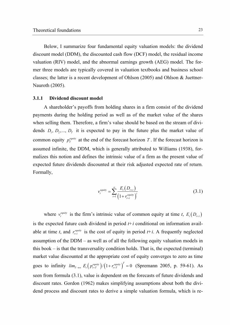
Below, I summarize four fundamental equity valuation models: the dividend discount model (DDM), the discounted cash flow (DCF) model, the residual income valuation (RIV) model, and the abnormal earnings growth (AEG) model. The for-mer three models are typically covered in valuation textbooks and business school classes; the latter is a recent development of Ohlson (2005) and Ohlson & Juettner-Nauroth (2005).

3.1.1 Dividend discount model

A shareholder’s payoffs from holding shares in a firm consist of the dividend payments during the holding period as well as of the market value of the shares when selling them. Therefore, a firm’s value should be based on the stream of divi-dends 1 2, ,..., TD D D it is expected to pay in the future plus the market value of

common equity equityTp at the end of the forecast horizon T . If the forecast horizon is

assumed infinite, the DDM, which is generally attributed to Williams (1938), for-malizes this notion and defines the intrinsic value of a firm as the present value of expected future dividends discounted at their risk adjusted expected rate of return. Formally,

( )( )1 1

t t iequityt iequityi t i

E Dv

r

∞+

= +

=+

∑ (3.1)

where equity

tv is the firm’s intrinsic value of common equity at time t, ( )t t iE D +

is the expected future cash dividend in period t+i conditional on information avail-able at time t, and equity

t ir + is the cost of equity in period t+i. A frequently neglected

assumption of the DDM – as well as of all the following equity valuation models in this book – is that the transversality condition holds. That is, the expected (terminal) market value discounted at the appropriate cost of equity converges to zero as time

goes to infinity ( ) ( ) / 1 0Tequity equity

T t t T t Tlim E p r→∞ + ++ = (Spremann 2005, p. 59-61). As

seen from formula (3.1), value is dependent on the forecasts of future dividends and discount rates. Gordon (1962) makes simplifying assumptions about both the divi-dend process and discount rates to derive a simple valuation formula, which is re-

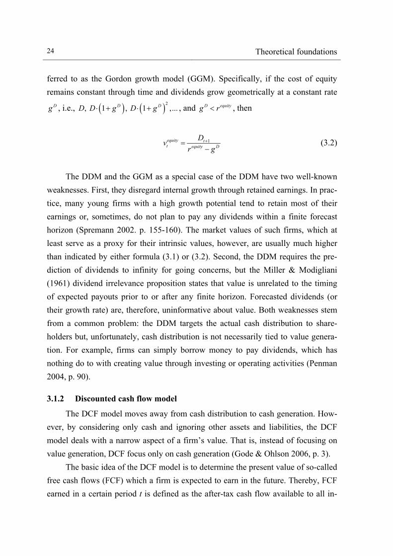
24 Theoretical foundations ferred to as the Gordon growth model (GGM). Specifically, if the cost of equity remains constant through time and dividends grow geometrically at a constant rate

Dg , i.e., ( ) ( )2, 1 , 1 ,...D DD D g D g⋅ + ⋅ + , and D equityg r< , then

1equity tt equity D

Dvr g

+=−

(3.2)

The DDM and the GGM as a special case of the DDM have two well-known

weaknesses. First, they disregard internal growth through retained earnings. In prac-tice, many young firms with a high growth potential tend to retain most of their earnings or, sometimes, do not plan to pay any dividends within a finite forecast horizon (Spremann 2002. p. 155-160). The market values of such firms, which at least serve as a proxy for their intrinsic values, however, are usually much higher than indicated by either formula (3.1) or (3.2). Second, the DDM requires the pre-diction of dividends to infinity for going concerns, but the Miller & Modigliani (1961) dividend irrelevance proposition states that value is unrelated to the timing of expected payouts prior to or after any finite horizon. Forecasted dividends (or their growth rate) are, therefore, uninformative about value. Both weaknesses stem from a common problem: the DDM targets the actual cash distribution to share-holders but, unfortunately, cash distribution is not necessarily tied to value genera-tion. For example, firms can simply borrow money to pay dividends, which has nothing do to with creating value through investing or operating activities (Penman 2004, p. 90).

3.1.2 Discounted cash flow model

The DCF model moves away from cash distribution to cash generation. How-ever, by considering only cash and ignoring other assets and liabilities, the DCF model deals with a narrow aspect of a firm’s value. That is, instead of focusing on value generation, DCF focus only on cash generation (Gode & Ohlson 2006, p. 3).

The basic idea of the DCF model is to determine the present value of so-called free cash flows (FCF) which a firm is expected to earn in the future. Thereby, FCF earned in a certain period t is defined as the after-tax cash flow available to all in-

Theoretical foundations 25

vestors of a firm: debt holders and equity holders. That is, FCF equals net operating profit after taxes (NOPAT) less the change in invested capital (i.e., the cumulative amount a firm has invested in its core operations). Unlike operating cash flow (OCF) reported in the cash flow statement, FCF itself is independent of financing and therefore not affected by capital structure; even though capital structure may affect a firm’s discount rate, the weighted average cost of capital ( waccr ) and there-fore its intrinsic value (Copeland, Koller & Murrin 2000, p. 167).

( )1 t tNOPAT EBIT tax rate= ⋅ − (3.3) The FCF can be calculated from information in financial statements. Koller, Goedhart & Wessels (2005) start with NOPAT calculated from the income state-ment using equation (3.3), add back depreciation and amortization, deduct increases in working capital, and deduct capital expenditures (CAPEX). Aboody (2006) pre-sents an alternative approach where FCF equals OCF less CAPEX plus interest net of income taxes. In this sense, FCF equals the amount of dividends, which a firm could pay if it had no debt and a full payout (i.e., a dividend payout ratio of one).

( )

& 1

t t t

t t t t

t t t

FCF NOPAT invested capitalNOPAT depreciation amortization working capital CAPEXOCF CAPEX interest tax rate

= −Δ= + −Δ −

= − + ⋅ −

(3.4)

In reality, firms use FCF to distribute dividends, pay debt holders, or simply retain the cash. Consequently, the present value of future FCF represents the intrin-sic value of common equity plus the market value of debt including preferred stock less cash & equivalents. We can also view future FCF as “firm dividends” and their present value as the value of the firm as a whole or entity value respectively. For-mally,

( )( )1 1

t t ientityt iwacci

E FCFv

r

∞+

=

=+

∑ (3.5)

26 Theoretical foundations

where entitytv is the entity value at time t, ( )t t iE FCF + is the expected future FCF

in period t+i conditional on information available at time t, and waccr is the weighted average cost of capital, indicated as a constant. From entity

tv , we must subtract the

market value of debt including preferred stock less cash & equivalents at time t (this subtotal is defined as the market value of net debt net debt

tp at time t) in order to re-

ceive the equity value equitytv at time t.

( )( )

1 1t t iequity net debt

t tiwacci

E FCFv p

r

∞+

=

= −+

∑ (3.6)

Such as the DDM and the GGM, the DCF model also has specific deficien-

cies. First, it is difficult to measure FCF, especially when the separation between operating, investing, and financing activities is blurry. For instance, when a retail bank receives deposits, it treats them as financing, which is per definition excluded from FCF. Arguably, taking deposits is part of a retail bank’s core business and should be an operating activity included in FCF.

Second, equation (3.4) identifies FCF as value added from selling services and products, but the negative treatment of investments (i.e., CAPEX) is troublesome. Anticipated investments made with ex ante positive net present values reduce FCF even if they create value. For extended horizons, the subsequent cash inflows of these investments are captured within the horizon and this ultimate matching of cash outflow and cash inflow captures the anticipated value added. However, for a firm as a going concern, investments roll over into new investments and the horizon may have to be very long to get this matching. Indeed, a lot of “good” firms have negative FCF for a long time as new investments exceed OCF each year (Penman & Sougiannis 1998, p. 350). What is more, the negative treatment of investments gives managers an arbitrary opportunity to manipulate FCF in the short term by delaying new investments.

Third, because FCF are not contemporaneous with value generation, it is diffi-cult to forecast them. Instead, DCF valuations typically start with a forecast of op-erating profit – basically an earnings forecast – and then account for actions, which

Theoretical foundations 27

affect the change in invested capital (Gode & Ohlson 2006, p. 4-5). This might also be one reason why sell-side analysts usually provide estimates of earnings rather than estimates of cash flows.

3.1.3 Residual income valuation model

In contrast, the RIV model derives forecasts for its key measure residual in-come (RI) – also referred to as abnormal earnings (AE) – directly from earnings forecasts. Ohlson (1995) defines residual income as 1

equityt t tRI NI r B −= − ⋅ (3.7)

where tRI is the residual income at time t, tNI denotes net income for the pe-

riod ending at time t, equityr is the cost of equity (assumed constant), and 1tB − is the

book value of common equity at time 1t − . The residual income is the amount that net income exceeds the capital charge on the book value of equity. The charge for the use of capital can be viewed as the opportunity cost of invested capital (Peasnell 1981, p. 54). Under the DDM, the intrinsic value of a firm’s equity equals the present value of future expected dividends. By using an accounting identity between dividends, net income, and changes in the book value of equity, the value of a firm can be re-expressed as the present value of a combination of net income and book value of equity. This accounting identity, called clean surplus relation, states that all changes in the book value of equity during a fiscal period are reflected in that period’s net income or dividends distributed to common shareholders (O’Hanlon & Peasnell 2002, p. 230-231). Formally, 1t t t tB B NI D−− = − (3.8)

where tB is the book value of common equity at time t, tNI is the net income

for the period from 1t − to t, and tD is the cash dividend paid to common share-

28 Theoretical foundations holders at time t. Ohlson (1995) shows that solving for tD in the clean surplus rela-

tion and substituting into the DDM formula (3.1) yields the RIV model,

( )( )1 1

t t iequityt t iequityi

E RIv B

r

∞+

=

= ++

∑ (3.9)

where again equity

tv is the intrinsic value of common equity at time t, tB is the

book value of common equity at time t, ( )t t iE RI + is the expected future residual

income in period t+i conditional on information available at time t, and equityr is the cost of equity, indicated as a constant. The RIV model moves away from the cash generating focus of the DCF model to book value of equity and net income. In their combination as residual income, they measure the generation of value. Lee (1996) demonstrates that the develop-ment of the RIV model parallels the concept of Economic Value Added (EVA) popularized by Stewart (1991) and today used by many large firms as the standard tool for value based management. Although the RIV model identifies residual in-come as a measure of a firm’s ability to create value, it has two major problems in practical applications. First, the clean surplus relation only holds if equity related capital transactions (e.g., issuance and buyback of shares, convertible bonds, em-ployee stock options) are value neutral and measured by their market values. In practice, capital transactions are often driven by market inefficiencies and thus have an impact on the value of a firm. Furthermore, both IFRS and U.S.-GAAP violate the market value condition for some capital transactions, such as convertible bonds when converted and employee stock options when exercised (Ohlson 2005, p. 328-329).

Second, RIV anchors on book values by deriving the intrinsic value of a firm as its book value of equity plus a premium for expected growth in the book value of equity (i.e., discounted future residual income). Such an emphasis on book values is only justified if they approximate market values reasonably well, as it is the case for financial assets and, more general, for firms in the financial industry. However, the focus on book values is misplaced in many other industries, especially when ac-

Theoretical foundations 29

counting is conservative (Gode & Ohlson 2006, p. 5). It is well to note that RIV does not conform to principles of equity valuation as we generally observe them in practice. Only few practitioners view current book value of equity as a starting point in valuation; the majority tends to focus on (future) earnings and earnings growth (Ohlson 2002, p. 248).

3.1.4 Abnormal earnings growth model

Although expected earnings and earnings growth are popular among analysts and investment bankers, theoretical cognition on earnings-based valuation is rare. The Ohlson (2005) and Ohlson & Juettner-Nauroth (2005) abnormal earnings growth (AEG) model legitimizes the common practice of using earnings estimates. Indeed, it shows how to convert analysts’ earnings forecasts to a valuation formula, which rely neither on the clean surplus relation nor on book value of equity. Given the clean surplus relation (and the notification) of equation (3.8), AEG at time t is equal to the change in residual income between 1t − and t (line one and two in equation (3.10)). For a constant cost of equity equityr , it is possible to express AEG without the book value of equity by rearranging terms.

( )( )( )

1

1 1 2

1 1 1 1 1

1 1 1 1 1

t t t

equity equityt t t t

equity equityt t t t t t

equity equity equity equityt t t t t t

t

AEG RI RI

NI r B NI r B

NI r B NI r B NI D

NI r B NI r B r NI r D

NI

−

− − −

− − − − −

− − − − −

= −

= − ⋅ − − ⋅

= − ⋅ − − ⋅ − +

= − ⋅ − + ⋅ − ⋅ + ⋅

= ( )1 11equity equityt tr D r NI− −+ ⋅ − + ⋅

(3.10)

Any firm as a going concern must eventually reach a steady state, where it does not earn abnormal earnings. Otherwise, per definition, its intrinsic value would be infinite. At this certain point in time 0tRI = and

1t

t equity

NIBr− = (3.11)

30 Theoretical foundations

Ohlson (2005) and Ohlson & Juettner-Nauroth (2005) utilize the RIV formula (3.9) together with identity (3.10) to derive the AEG valuation model, which is mathematically equivalent to the RIV model. Formally,

( ) ( ) ( )1

2

1 1it t iequity equity

t t t iequity equityi

E NIv r E AEG

r r

∞ −++

=

⎡ ⎤= + ⋅ + ⋅⎢ ⎥⎣ ⎦∑ (3.12)

where equity

tv is the intrinsic value of common equity at time t, ( )1tE NI + is the

expected net income in period t+i, ( )t t iE AEG + is the expected growth in abnormal

earnings in period t+i both conditional on information available at time t, and equityr is the cost of equity, indicated as a constant.

From a theoretical point of view, the AEG model embeds two distinct advan-tages compared to the RIV model. First, we obtain a valuation, which is equivalent to the RIV framework, but without having to forecast book value of equity; the bal-ance sheet drops out. Growth in book value of equity, modeled under RIV, is sim-ply net income minus dividends. Hence, by forecasting net income and dividends, that is, abnormal earnings growth, the change in book value is redundant. Second, although derived from the clean surplus relation, the AEG model in formula (3.12), eventually, does not require clean surplus accounting (Penman 2005, p. 369-370). Practically orientated, the AEG model coincides with investment practice where equity valuation revolves around earnings and their subsequent growth (Ohlson 2005, p. 342). As any fundamental equity valuation model, the AEG also comes with some reservations. Technically, Ohlson (2005) and Ohlson & Juettner-Nauroth (2005) set

( ) / equityt t t iB E NI r+= arbitrarily. However, in reality, no economic justification exists

to start a valuation at the steady state, and then to allow for abnormal earnings in subsequent periods. What is more, ( ) / equity

t t iE NI r+ , the anchor in the AEG model, is

not actually a number which can be found in the financial statements. It is a fore-cast, based on speculation. In contrast, RIV follows the fundamentalists’ dictate to distinguish what is known (in the financial statements) from speculation, by anchor-ing on book value of equity and then adding speculation about future residual in-

Theoretical foundations 31

come. Besides that, no empirical evidence on the performance neither for the AEG model nor its simplification as proposed in Ohlson & Juettner-Nauroth (2005) exist so far.

Taking the practical limitations of the presented fundamental equity valuation models into account, it is difficult to argue that practitioners ought to rely on either the DDM, DCF, RIV, or AEG method when it comes to real world applications. In fact, we now understand why so many practitioners revert to the market-based mul-tiples valuation approach.

3.2 Derivation of intrinsic multiples

In general, the valuation literature discusses two broad approaches to estimat-ing the value of firms. The first is fundamental equity valuation, in which the value of a firm is estimated directly from its expected future payoffs without appeal to the current market value of other firms. Fundamental equity valuation models are based on dividends, (free) cash flows, or (abnormal) earnings, and involve the computa-tion of the present value of expected future payoffs – explained before for the DDM, DCF, RIV, and AEG method.11 The second is market-based valuation, in which value estimates are obtained by examining market values of comparable firms. This approach involves applying a synthetic market multiple (e.g., the P/E multiple) from the comparable firms to the corresponding value driver (e.g., earn-ings) of the firm being valued to secure a value estimate (Bhojaj & Lee 2002, p. 413-414).12

In market-based valuation, sometimes also referred to as relative valuation, a target’s firm value equals the product of a synthetic peer group multiple and the tar- 11 This book does not discuss liquidation valuation, in which a firm is valued at the “break-up” value of its asset. Commonly used in valuing firms in financial distress, this fundamental equity valuation method is not appropriate for most going concerns (Bhojraj & Lee 2002, p. 413). 12 A third approach, not covered in this book, is contingent claim valuation based on option pricing theory. Interested readers may refer to standard corporate finance textbooks such as Brealy & Myers (2000) chapter 21, Damodaran (2001) chapter 11, Copeland, Weston & Shastri (2004) chap-ter 9, Koller, Goedhart & Wessels (2005) chapter 20, or Spremann (2005) chapter 8 to get a basic understanding.

32 Theoretical foundations get firm's corresponding value driver. In doing so, the value driver in question is treated as a summary statistic for the value of the firm. Assuming the target firm in its current state “deserves” the same market multiple as the “typical” firm of the peer group, this procedure allows to estimate what the market would pay for the target firm (Bhojraj, Lee & Ng 2003, p. 12). But, which are the firms that deserve the same multiple as the target firm? Fundamental analysis helps to resolve this question. In fact, explicit expressions for most of the commonly used multiples can be derived using either the DDM, DCF, or RIV method and a few additional as-sumptions. These expressions also make it easier to interpret observed patterns in multiples, such as why growth firms and industries have higher earnings multiples than stable firms and industries. In the following, I present such explicit expressions of the P/E, the EV/EBIT, and the P/B multiple. Because these multiples are deriva-tions of fundamental equity valuation models, which aim at estimating the intrinsic value of a firm, they are called “intrinsic” multiples.

3.2.1 Intrinsic P/E multiple derived from the DDM

The starting point to relate the P/E multiple to fundamental analysis is the GGM. As a special case of the more general DDM, the GGM converts a constantly growing infinite stream of dividends to the value of a firm. By assuming a constant payout ratio (PR), dividends at time t are a fixed proportion of net income at time t t tD PR NI= ⋅ (3.13)

Net income for one year ahead 1tNI + is determined by current net income tNI

and its (constant) growth rate NIg

( )1 1 NIt tNI NI g+ = ⋅ + (3.14)

Thus, ( )1 1 NIt tD PR NI g+ = ⋅ ⋅ + (3.15)

Substituting equation (3.15) into the GGM formula (3.2), yields

Theoretical foundations 33

( )1 NI

tequityt equity NI

PR NI gv

r g⋅ ⋅ +

=−

(3.16)

Dividing both sides of equation (3.16) by net income, eventually leads to the

intrinsic P/E multiple at time t

( )1 NIequity

tequity NI

t

PR gvNI r g

⋅ +=

− (3.17)

A closer look at equation (3.17) reveals the fundamental determinants of the

P/E multiple. Under the given assumptions, the P/E multiple is positively related to future (earnings) growth and negatively related to risk, as measured by the cost of equity (Beaver & Morse 1978, p. 65-66). According to equation (3.17), a high divi-dend payout ratio also has a positive impact on the P/E multiple. However, Thomas & Zhang (2004) show that this impact is a minor one.

3.2.2 Intrinsic EV/EBIT multiple derived from the DCF model

The EV/EBIT multiple gained popularity recently, especially among invest-ment bankers. Although a bit more complex than the derivation of the intrinsic P/E multiple, it is possible to derive an intrinsic EV/EBIT multiple from the DCF valua-tion model. However, the two main assumptions are similar: NOPAT grows at a constant rate year by year and the proportion of NOPAT a firm re-invests each year is fixed. Together, this means that FCF also grow at a constant rate FCFg year by

year (Koller, Goedhart & Wessels 2005, p. 62). Using the same perpetuity relation-ship as in the GGM, the entity value of a firm in the DCF formula (3.5) can be re-written as

1entity tt wacc FCF

FCFvr g

+=−

(3.18)

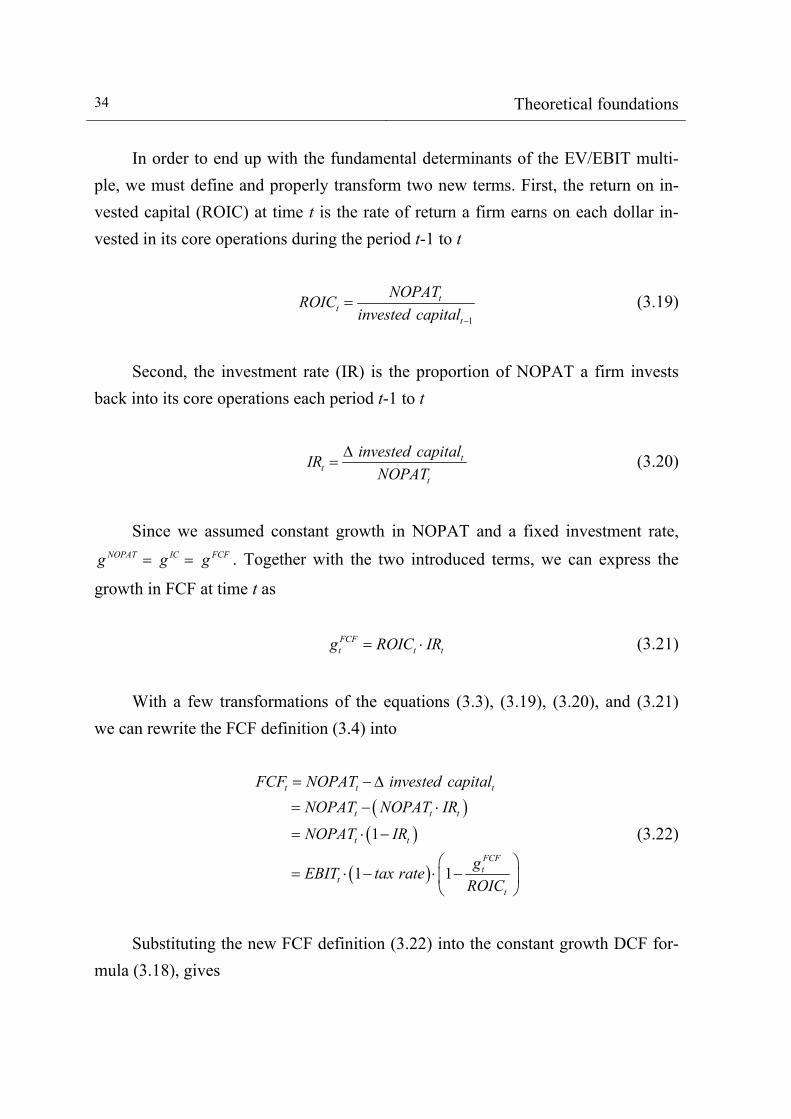
34 Theoretical foundations

In order to end up with the fundamental determinants of the EV/EBIT multi-ple, we must define and properly transform two new terms. First, the return on in-vested capital (ROIC) at time t is the rate of return a firm earns on each dollar in-vested in its core operations during the period t-1 to t

1

tt

t

NOPATROICinvested capital −

= (3.19)

Second, the investment rate (IR) is the proportion of NOPAT a firm invests

back into its core operations each period t-1 to t

tt

t

invested capitalIRNOPAT

Δ= (3.20)

Since we assumed constant growth in NOPAT and a fixed investment rate,

NOPAT IC FCFg g g= = . Together with the two introduced terms, we can express the

growth in FCF at time t as FCF

t t tg ROIC IR= ⋅ (3.21)

With a few transformations of the equations (3.3), (3.19), (3.20), and (3.21)

we can rewrite the FCF definition (3.4) into

( )( )

( )

1

1 1

t t t

t t t

t t

FCFt

tt

FCF NOPAT invested capitalNOPAT NOPAT IR

NOPAT IR

gEBIT tax rateROIC

= −Δ

= − ⋅

= ⋅ −

⎛ ⎞= ⋅ − ⋅ −⎜ ⎟

⎝ ⎠

(3.22)

Substituting the new FCF definition (3.22) into the constant growth DCF for-

mula (3.18), gives

Theoretical foundations 35

( )1 1 1

FCF

ttentity

t wacc FCF

gEBIT tax rateROIC

vr g

+

⎛ ⎞⋅ − ⋅ −⎜ ⎟

⎝ ⎠=−

(3.23)

Finally, dividing both sides of equation (3.23) by current tEBIT , yields the in-

trinsic EV/EBIT multiple at time t 13

( ) ( )1 1 1

FCFFCF

entitytt

wacc FCFt

gg tax rateROICv

EBIT r g

⎛ ⎞+ ⋅ − ⋅ −⎜ ⎟

⎝ ⎠=−

(3.24)

As equation (3.24) shows, the EV/EBIT multiple is determined by four fac-tors: growth (in FCF) and profitability, measured by ROIC, have a positive effect on the EV/EBIT multiple, whereas taxes and risk, measured by the weighted aver-age cost of capital, have a negative effect. Based on equation (3.17) and (3.24), we can conclude that, all other things equal, firms with higher growth rates and lower risk should trade at a higher P/E and EV/EBIT multiple than firms without these characteristics. In other words, if the market value of equity approximates the pre-sent value of future payoffs, growth and risk should explain a significant portion of the cross-sectional variation in the P/E and EV/EBIT multiple.

3.2.3 Intrinsic P/B multiple derived from the RIV model

The P/B multiple is common for valuing banks and, more generally, for firms in the financial industry. The intrinsic P/B multiple can be derived from the RIV model. To do so, we suppose residual income to grow at a constant rate RIg each

year.14 This assumption also implies constant growth in dividends and book value of

13 The derivation of the intrinsic EV/EBIT multiple is based on different passages of Koller, Goedhart & Wessels (2005). 14 Fairfield (1994) and Penman (1996) also derive the intrinsic P/B multiple from the RIV model. In contrast to the methodology presented in this book, they do not use the assumption of constant RI growth. The interpretation of the result, however, is identical.

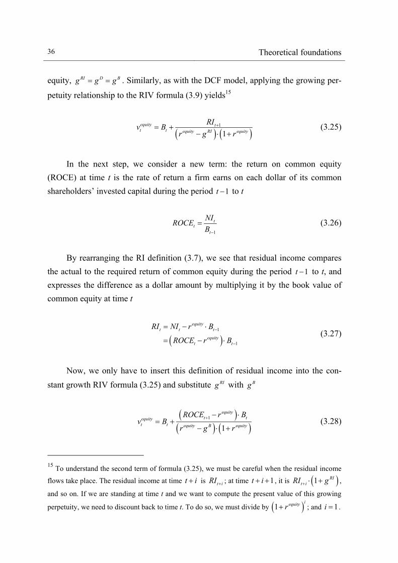
36 Theoretical foundations equity, RI D Bg g g= = . Similarly, as with the DCF model, applying the growing per-

petuity relationship to the RIV formula (3.9) yields15

( ) ( )

1

1equity tt t equity RI equity

RIv Br g r

+= +− ⋅ +

(3.25)

In the next step, we consider a new term: the return on common equity

(ROCE) at time t is the rate of return a firm earns on each dollar of its common shareholders’ invested capital during the period 1t − to t

1

tt

t

NIROCEB −

= (3.26)

By rearranging the RI definition (3.7), we see that residual income compares the actual to the required return of common equity during the period 1t − to t, and expresses the difference as a dollar amount by multiplying it by the book value of common equity at time t

( )1

1

equityt t t

equityt t

RI NI r B

ROCE r B−

−

= − ⋅

= − ⋅ (3.27)

Now, we only have to insert this definition of residual income into the con-

stant growth RIV formula (3.25) and substitute RIg with Bg

( )( ) ( )

1

1

equityt tequity

t t equity B equity

ROCE r Bv B

r g r+ − ⋅

= +− ⋅ +

(3.28)

15 To understand the second term of formula (3.25), we must be careful when the residual income

flows take place. The residual income at time t i+ is t iRI + ; at time 1t i+ + , it is ( )1 RIt iRI g+ ⋅ + ,

and so on. If we are standing at time t and we want to compute the present value of this growing

perpetuity, we need to discount back to time t. To do so, we must divide by ( )1iequityr+ ; and 1i = .

Theoretical foundations 37

and, eventually, divide both sides of the equation (3.28) by tB to receive the

intrinsic P/B multiple at time t

( )

( ) ( )11

1

equityequitytt

equity B equityt

ROCE rvB r g r

+ −= +

− ⋅ + (3.29)

Equation (3.29) shows that a firm’s P/B multiple is a function of its expected profitability, measured by ROCE, its risk, measured by the cost of equity, and its growth (in book value of equity). Also, note that if a firm is expected to earn zero residual income in the future (i.e., 1 0equity

tROCE r+ − = ), its intrinsic P/B multiple is

one (i.e., / 1equityt tv B = ) and thus the firm is worth exactly its current book value of

equity. Penman (1996) refers to this benchmark case as the “normal” P/B multiple. Any premium to the book value of equity, at which a firm trades, is attributable to expected non-zero residual income and growth in book value. Thus, the P/B multi-ple is a useful measure to get a quick impression of what the market thinks about the key value drivers of a firm: growth, profitability, and risk. When comparing the fundamental determinants of the P/E and the P/B multi-ple, we find that both of them depend on the risk of a firm, measured by its cost of equity. However, the P/E multiple is mainly driven by future earnings growth, whereas the major drivers of the P/B multiple are future ROCE and growth in book value of equity (Penman 1996, p. 256). Given the importance of the P/B multiple in the financial industry and its underlying drivers, we might understand why execu-tives of many banks tend to worry more about being profitable and becoming “big” than focusing solely on earnings (growth) as it is common in other industries, espe-cially, of course, in growth industries.

38 Theoretical foundations

Figure 3.1: Intrinsic multiples derived from fundamental valuation models

Intrinsic P/E multiple Intrinsic EV/EBIT multiple Intrinsic P/B multiple

Valuation model

Valuation formula

Simplified formula

Intrinsic multiple

DDM DCF model RIV model

( )( )1 1

t t iequityt iequityi t i

E Dv

r

∞+

= +

=+

∑

1equity tt equity D

Dvr g

+=−

( )( )1 1

t t ientityt iwacci

E FCFv

r

∞+

=

=+

∑ ( )( )1 1

t t iequityt t iequityi

E RIv B

r

∞+

=

= ++

∑

( )1 NIequityt

equity NIt

PR gvNI r g

⋅ +=

−

1entity tt wacc FCF

FCFvr g

+=−

( ) ( )1 1 1FCF

FCFentity

ttwacc FCF

t

gg tROICv

EBIT r g

⎛ ⎞+ ⋅ − ⋅ −⎜ ⎟

⎝ ⎠=−

( ) ( )1

1equity tt t equity RI equity

RIv Br g r

+= +− ⋅ +

( )( ) ( )

111

equityequitytt

equity B equityt

ROCE rvB r g r

+ −= +

− ⋅ +

Intrinsic P/E multiple Intrinsic EV/EBIT multiple Intrinsic P/B multiple

Valuation model

Valuation formula

Simplified formula

Intrinsic multiple

DDM DCF model RIV model

( )( )1 1

t t iequityt iequityi t i

E Dv

r

∞+

= +

=+

∑

1equity tt equity D

Dvr g

+=−

( )( )1 1

t t ientityt iwacci

E FCFv

r

∞+

=

=+

∑ ( )( )1 1

t t iequityt t iequityi

E RIv B

r

∞+

=

= ++

∑

( )1 NIequityt

equity NIt

PR gvNI r g

⋅ +=

−

1entity tt wacc FCF

FCFvr g

+=−

( ) ( )1 1 1FCF

FCFentity

ttwacc FCF

t

gg tROICv

EBIT r g

⎛ ⎞+ ⋅ − ⋅ −⎜ ⎟

⎝ ⎠=−

( ) ( )1

1equity tt t equity RI equity

RIv Br g r

+= +− ⋅ +

( )( ) ( )

111

equityequitytt

equity B equityt

ROCE rvB r g r

+ −= +

− ⋅ +

3.3 Market multiples

3.3.1 Definition and categorization of market multiples

Intrinsic multiples help to form a decent understanding of a multiple’s funda-mental drivers. However, when people talk about multiples, they usually do not think of intrinsic multiples. What they have in mind are market multiples. That is, the market value (i.e., price), not the intrinsic value, determines the size of a certain multiple. In accordance to Penman (2004), a (market) multiple is defined as “the ratio of a market price variable to a particular value driver of a firm.” Hence, multi-ples are summary measures, which inform about the market’s opinion of a firm’s market valuation compared to its competitors.

Using market value in the numerator distinguishes multiples from “financial ratios,” which provide information on a firm’s financial and operating performance

Theoretical foundations 39

(e.g., growth, profitability, leverage, or liquidity).16 Hence, although terms such as “price-earnings ratio” or “price to book ratio” are very common, I prefer using the more precise terms “price to earnings multiple” and “price to book value (of com-mon equity) multiple” to avoid misinterpretations.

Figure 3.2: Categorization of multiples

Accrual flowmultiples

Book valuemultiples

Cash flowmultiples

Alternativemultiples

Forward-lookingmultiples

P / SA P / TA P / OCF

PEG

P / SA 1P / GI P / IC P / D

P / (EBIT+R&D)P / SA 2

P / EBITDA P / BP / (EBIT+AIA)

P / EBITDA 1P / EBIT

P / (EBIT+KC)P / EBITDA 2

P / EBTP / (E+R&D)

P / EBIT 1P / E

P / (E+AIA)P / EBIT 2P / (E+KC)P / EBT 1P / EBT 2

P / E 1P / E 2

EV / SA EV / TA EV / OCF EV / (EBIT+R&D) EV / SA 1EV / GI EV / IC EV / (EBIT+AIA) EV / SA 2

EV / EBITDA EV / (EBIT+KC) EV / EBITDA 1EV / EBIT EV / EBITDA 2

EV / EBIT 1EV / EBIT 2

Ent

ity v

alue

mul

tiple

sE

quity

val

uem

ultip

les

Accrual flowmultiples

Book valuemultiples

Cash flowmultiples

Alternativemultiples

Forward-lookingmultiples

P / SA P / TA P / OCF

PEG

P / SA 1P / GI P / IC P / D

P / (EBIT+R&D)P / SA 2

P / EBITDA P / BP / (EBIT+AIA)

P / EBITDA 1P / EBIT

P / (EBIT+KC)P / EBITDA 2

P / EBTP / (E+R&D)

P / EBIT 1P / E

P / (E+AIA)P / EBIT 2P / (E+KC)P / EBT 1P / EBT 2

P / E 1P / E 2

EV / SA EV / TA EV / OCF EV / (EBIT+R&D) EV / SA 1EV / GI EV / IC EV / (EBIT+AIA) EV / SA 2

EV / EBITDA EV / (EBIT+KC) EV / EBITDA 1EV / EBIT EV / EBITDA 2

EV / EBIT 1EV / EBIT 2

Ent

ity v

alue

mul

tiple

sE

quity

val

uem

ultip

les

Source: author based on Richter (2005), p. 83 and Krolle, Schmitt & Schwetzler (2005), p. 16. Legend: P = (stock) price / market capitalization, EV = enterprise value, SA = sales / revenues, GI = gross income, EBITDA = earnings before interest, taxes, depreciation, and amortization, EBIT = earnings before interest and taxes, EBT = earnings before taxes / pre-tax income, E = earnings / net income available to common shareholders, TA = total assets, IC = invested capital, B = book value of common equity, OCF = operating cash flow, D = (ordinary cash) dividend, R&D = research & development expenditures, AIA = amortization of intangible assets, KC = knowledge costs = R&D + AIA, and PEG = price to earnings to earnings growth ratio. Forward-looking multiples are based on mean consensus analysts’ forecasts for the next two years (1 = one year, 2 = two years) provided by I/B/E/S. The multiples shown within this two dimensional categorization framework are just a selection of the universe of possible multiples. However, any multiple can be classified within this framework.

16 E.g., Palepu, Healy & Bernard (2000) chapter 9, Harrington (2004) chapter 1, Lundholm & Sloan (2004) chapter 5, or Penman (2004) chapter 11 and 12 give a good overview of financial ratios used in practice. See also subsection 4.5.1.

40 Theoretical foundations

The loose definition of multiples, theoretically, allows calculating a huge number of different multiples for a given firm. Although practitioners do not com-pute any possible multiple, the list of multiples used is long and diverse (Löhnert & Böckmann 2005, p. 405). In order to get an overview, it makes sense to establish a categorization framework. Frequently, authors categorize multiples based on either the market price variable or the type of value driver used to construct the multiples. If we also want to analyze specific characteristics of certain types of multiples, a two dimensional categorization scheme, as shown in figure 3.2, is benefical. In the first dimension, the scheme focuses on the numerator of a multiple and differenti-ates between equity value and entity value multiples. Equity value multiples are based on the stock price or the market capitalization of a firm, whereas entity value multiples are based on the enterprise value of a firm. Formally, an equity value mul-tiple ,

equityi tλ of firm i at time t is

,,

,

equityi tequity

i ti t

px

λ = (3.30)

where ,

equityi tp is the current market value of common equity and ,i tx is the un-

derlying value driver of the multiple. Similarly, an entity value multiple ,entityi tλ of the

same firm at time t can be written as

, , ,,

, ,

ˆentity equity net debti t i t i tentity

i ti t i t

p p px x

λ+

= = (3.31)

where ,

entityi tp is the current enterprise value which equals the sum of the market

value of common equity ,equityi tp and an estimator of the market value of net debt

,ˆ net debt

i tp , and ,i tx is again the value driver.17

17 Net debt is defined as total debt less cash & equivalents plus preferred stock. Since the market value of net debt net debtp is usually not publicly available, I approximate net debtp with the book

Theoretical foundations 41

The origin of the value driver ,i tx in the financial statement constitutes the

main differentiation criteria for the second dimension of the categorization frame-work, where I distinguish accrual flow, book value, cash flow, alternative, and for-ward-looking multiples.18 The proposed framework offers high flexibility, because it is possible to classify any multiple within this scheme. Below, an overview ex-plains the characteristics of the most common equity value and entity value multi-ples as well as of some alternative multiples and discusses the difference between trailing and forward-looking multiples.

3.3.2 Common equity value and entity value multiples

3.3.2.1 Price to earnings multiple. Much of the real world discussion of firms’ eq-uity market values concentrates on the P/E multiple, which gained popularity in the early 1930s with the introduction of the value investing style by Benjamin Graham (Spremann 2005, p. 327). Although the P/E multiple is part of any multiples valua-tion in practice, at least for marketing or plausibility purposes, it comes with three substantial drawbacks. First, the P/E multiple does not have any meaning if a firm has a negative or low net income (Pereiro 2002, p. 253). Second, as the bottom line number in the income statement, different accounting policies affect net income the most of all numbers in financial statements. Third, such as with all other equity value multiples, managers can arbitrarily lever up the P/E multiple by changing the capital structure of the firm and putting on additional debt (Frykman & Tolleryd 2003, p. 62-64).19 Hence, from a theoretical point of view, using the P/E multiple is appropriate in industries where firms report solid earnings, are subject to uniform accounting policies, and operate with similar capital structures. Despite of its short-

value of net debt net debtb and write ˆ net debtp to indicate the approximation (Koller, Goedhart & Wessels 2005, p. 347-348). 18 Another type of multiples, not covered in this book, can be non-financial multiples. As the name implies the scaling variable of such multiples is non-financial information obtained from outside of the financial statements. Although theoretical arguments in favor of non-financial multiples in cer-tain industries or stages of an industry exist, limits of data availability and objectivity make it diffi-cult to apply non-financial multiples in practice. See Damodaran (2001) chapter 11 or Damodaran (2002) chapter 20 for an overview of some non-financial multiples. 19 See subsection 4.2.1 on how capital structure affects equity value multiples.

42 Theoretical foundations comings, the P/E multiple is still the most popular multiple and will continue to at-tract attention from market participants because simply everyone uses it.

3.3.2.2 Price to book multiple. The P/B multiple, also known as market to book value of equity multiple, is best used on firms in capital-intensive industries (e.g., oil & gas or financials) where tangible (financial) assets are the source of value generation (Frykman & Toleryd 2003, p. 65). However, the use of the P/B multiple with industrial firms requires care because reported numbers for assets are based on historical costs, which are typically an unreliable indicator of economic value. Fur-thermore, the P/B multiple does not reflect a firm’s earnings power or cash flows. Therefore, Suozzo, Cooper, Sutherland & Deng (2001) suggest to view the P/B multiple together with return on common equity. This seems also to be useful be-cause of their fundamental linkage. Other analysts favor the P/B multiple because book values are relatively constant, which eases comparability over time. The P/B multiple or its reciprocal are also popular in two related contexts. First, “value in-vestors” such as Warren Buffet use the P/B multiple as a coarse filter to detect “cheap” stocks, which might be undervalued. Second, the book to market value of equity ratio constitutes one of the two systematic factors in the Fama-French three-factor model, which is the state-of-the-art model to determine firms’ appropriate cost of capital (i.e., equityr and waccr ) in the hedge funds and private equity industry.20

3.3.2.3 Enterprise value to sales multiple. Dividing the enterprise value of a firm by its sales or revenues is a way of comparing firms in cyclical industries, where net income and EBIT are frequently negative during the down part of an industry cycle, or young industries, where firms typically have lower margins and typically invest more than they earn in the first years in order to ensure future growth (Geddes 2003, p. 83). Besides that, sales are subject to less accounting idiosyncrasies of individual firms compared to other numbers in financial statements. The main problem of the EV/SA and the P/SA multiple (the equivalent equity value multiple) stems from the 20 Fama & French (1992) find that historical average returns on stocks of small firms and on stocks with high ratios of book to market value of equity are higher than predicted by the beta in the capi-tal asset pricing model (CAPM). Based on these observations, they develop a three-factor model, which captures the cross-section of average returns on U.S. (Fama & French 1993 and 1995) and international stocks (Fama & French 1998).

Theoretical foundations 43

fact that when using them, the market price variable is scaled by the top number in the income statement. Such a scaling ignores all information on the operating effi-ciency of a firm contained in the numbers further down in the income statement (Benninga & Sarig 1997, p. 326-327). Nevertheless, both multiples gained consid-erable attention during the rise of technology and internet stocks in the mid and late 1990s, but lost proponents since the dot-com bubble burst in 2001. The intuition underlying sales multiples is that, within an industry, the gross margins and the op-erating efficiency are similar among firms; unfortunately, this is typically not the case in reality.

3.3.2.4 Enterprise value to EBIT(DA) multiple. These two multiples became the darlings of investment bankers when preparing pitch books for industry deals in the recent past (Evans & Bishop 2001, p. 166). Indeed, several reasons speak in favor of the EV/EBITDA and the EV/EBIT multiple. As entity value multiples, they are less affected by capital structure decisions than equity value multiples.21 Further-more, both multiples measure operating performance and are not affected by differ-ent tax rules. Additionally, EBITDA represents a proxy for cash flows and is free of arbitrariness concerning the accounting for depreciation and amortization. If the capital intensity (i.e., depreciation expenditures as a percentage of EBITDA) varies within an industry, using EBIT is advantageous (Löhnert & Böckmann 2005, p. 412-413). However, both multiples leave out information further down in the in-come statement such as income from minority holdings or cash earnings (Damoda-ran 2006, ch. 12, p. 5-6). They also ignore the opportunity managers have to add value through skilled tax management.

3.3.3 Alternative multiples

The multiples we concentrated on so far are not only the most prevalent but also the most obvious multiples. That is, because the underlying value drivers of these multiples – net income, book value of equity, sales, and EBIT(DA) – are im-portant line items in the financial statements of any firm. Numbers in the financial statements, however, are “conservative” because they must comply with the reli-

21 See subsection 4.2.1.

44 Theoretical foundations ability criterion of accounting. The reliability criterion demands that assets and li-abilities be recognized only if they can be measured with reasonable precision and supported by objective evidence, free of opinion and bias (Gibson 1998, p. 16). The balance sheet tends to omit value and the income statement does not recognize all the value that is added for the shareholders. From this perspective, the common value drivers used for the construction of multiples are a suboptimal choice.

Another issue is that multiples are summary measures of a firm’s ability to create future payoffs for shareholders. They simply compress information on the key value drivers – future growth, profitability, and risk – into a single number. Across firms, this is insofar problematic as even firms of comparable size and within the same industry may have different growth rates. Therefore, using multi-ples without adjustments for future growth potential is likely to produce inaccurate valuation results (Arzac 2005, p. 70-71). In the following two subsections, I present alternative multiples to overcome the deficiencies of common multiples.

3.3.3.1 Knowledge-related multiples. In the literature, several definitions of ac-counting conservatism exist. Basu (1997), for instance, defines accounting conser-vatism as the practice of writing down assets and thereby reducing earnings in re-sponse to bad news, but not writing up assets and increasing earnings in response to good news. Similarly, Gjesdal (1999) distinguishes economic profitability from ac-counting profitability. He characterizes accounting as conservative if it assigns in-vestments a carrying value that yields an expected accounting return greater than the internal rate of return on their cost. Thus, conservative accounting carries an asset whose value is equal to its historical cost (i.e., a zero net present value invest-ment) at less than historical cost, as it is the case with R&D investments.

Nowadays, investing in R&D is a major productive input for a large number of firms, particularly those operating in science and technology related industries. From an accounting perspective, however, R&D differs from other capital inputs such as property, plant and equipment, inventory, or project financing (Aboody & Lev 2000, p. 2748). While most accounting standards mandate the capitalization and periodic depreciation of the latter forms of long-term investment, R&D is im-mediately expensed in financial statements, which produces “low quality” earnings numbers. By examining the value relevance of R&D, several recent studies provide

Theoretical foundations 45

striking evidence to view R&D as an investment rather than an expense.22 Conse-quently, adding back R&D expenditures to EBIT or net income yields “higher qual-ity” earnings.

If accounting standards change and firms capitalize R&D, it would appear as an intangible asset on the balance sheet. Following the definition of Swiss-GAAP, Pfeil (2004) defines intangible assets as non-monetary assets without physical exis-tence. Even if they are intangible, they are nevertheless valuable resources, repre-senting future payoffs. Likewise, Lev (2001) describes intangible assets as a non-physical source of value generation. Examples of assets without physical substance are brand names, copyrights, goodwill, leasehold rights, licenses, patents, or soft-ware. Due to high M&A activity in the late 1990s and again since 2003, goodwill, defined as the difference between the purchase price and the target firm’s net asset value, forms a large portion of many firms’ total assets today. Conceptually, good-will is an all-encompassing repository for non-recognizable intangible assets incor-porating the capacity for generating future payoffs (Johnson & Petrone 1998, p. 297-298). Hitherto, all international accounting standards but U.S.-GAAP mandate the amortization of capitalized intangible assets (AIA) over their expected “useful” lives (White, Sondhi & Fried 2003, p. 264).23 For many intangible assets, however, law or regulation prescribes the useful amortization time based on conservative ac-counting. Consequently, reported amortization expenditures overestimate the effec-tive decrease – if there is any decrease – in the value of intangible assets.

Both the immediate expense of R&D and the principle of systematic amortiza-tion of intangible assets decrease the quality of reported earnings and consequently the quality of multiples based on earnings numbers. To correct the negative conse-quences of accounting conservatism on earnings and to produce a more reliable pic-ture of a firm’s true economic success, I suggest adding back R&D expenditures and/or amortization to EBIT and net income in all industries with a substantial ex-

22 E.g., Amir & Lev (1996), Lev & Sougiannis (1996), Aboody & Lev (1998 and 2000), Chan, Lakonishok & Sougiannis (2001), Lev & Thomas (2002), Eberhart, Maxwell & Siddique (2004), Guo, Lev & Shi (2006), or Nelson (2006). 23 Under U.S.-GAAP, SFAS 142, which became effective in 2002, eliminates the systematic amor-tization of acquisition goodwill and requires firms to periodically test their goodwill for possible impairment losses (White, Sondhi & Fried 2003, p. 526-527).

46 Theoretical foundations posure to intangible assets. The “and/or” decision depends on the magnitude (or existence) and consistency of R&D expenditures and amortization within an indus-try. That is, if R&D expenditures (amortization costs) are relatively low or come with high volatility, we are better off adding back only amortization (R&D expendi-tures). On the other hand, if both numbers are of considerable size and stable, we should sum them up into a single number.

The source of future payoffs R&D investments and intangible assets can gen-erate is human knowledge (Lev 2001, p. 5). In this spirit, I define the sum of R&D expenditures and amortization of intangible assets as costs for the creation and maintenance of intangible assets or short knowledge costs (KC). By adopting these knowledge adjustments to the multiples valuation method, I identify the following knowledge-related multiples: EV/(EBIT+R&D), EV/(EBIT+AIA), EV/(EBIT+KC), P/(EBIT+R&D), P/(EBIT+AIA), P/(EBIT+KC), and P/(E+R&D), P/(E+AIA), P/(E+KC).

3.3.3.2 Price to earnings to earnings growth multiple. In recent years, the price to earnings to earnings growth (PEG) multiple became well-known. As the name im-plies the PEG multiple is equal to a P/E multiple divided by an earnings growth rate. Analysts differ in their choice of the form of the P/E multiples (i.e., price to trailing earnings or price to forward earnings) and in their choice of the earnings growth rate ranging from a one-year historical growth rate to an average expected annual growth rate estimated for several years in the future (Easton 2004b, p. 77).

Many analysts use the PEG multiple to assess whether a firm’s P/E multiple – the multiple, which typically forms the basis of their stock recommendations – is “out of line.” According to Lynch (2000), who argues that the P/E multiple of any firm that is correctly priced should equal its earnings growth rate, a firm’s fair PEG multiple is equal to one. Hence, the rule of thumb would be to hold firms with a PEG multiple around one, and to sell (buy) firms with a PEG multiple considerably greater (less) than one (Bradshaw 2004, p. 33). This rule of thumb may be useful for screening a stock universe or checking the plausibility of valuations, however, ac-tual investment decisions require the application of a valuation model.

The underlying assumption of the PEG multiple is that P/E multiples are posi-tively linearly correlated to the growth rate in earnings (Suozzo, Cooper, Sutherland

Theoretical foundations 47

& Deng 2001, p. 39-40). However, this assumption is unrealistic because it implies that firms with constant profits – no matter if high or low – have an undefined value. Nevertheless, at high growth rates, PEG multiples are stable and less sensi-tive to changes in growth, which makes them more suitable for valuing firms in high growth industries, but only under the precondition that the industry already reached the stage where firms are profitable. Although uncommon, an alternative is to express the PEG multiple on an enterprise level by using EV as market price variable, EBIT as value driver, and EBIT growth as growth variable (Koller, Goedhart & Wessels 2005, p. 386).

3.3.4 Trailing and forward-looking multiples

When building a multiple, the numerator always refers to the latest available number of the market price variable used. In the standard multiples approach, the value driver in the denominator also refers to the latest numbers, which we typically find in the financial statements for the most recent fiscal quarter or year. Such mul-tiples are called trailing multiples because the numbers used are based on historical data. Except for the PEG multiple, all other multiples we discussed so far are typi-cally calculated and reported as trailing multiples. If the value driver of a multiple refers to a forecast – typically a one-year or two-year forecast – instead of a histori-cal number, it is termed a forward-looking or leading multiple (Benninga & Sarig 1998, p. 312).

Valuation theory tells us that the value of a firm equals its discounted stream of expected future payoffs. Following this principle, forward-looking multiples are more appropriate for valuation purposes. In practice, the difficulty with forward-looking multiples is that we must collect the value driver estimates for all firms within the peer group. For an analyst covering a whole industry, this is not a major problem because she can utilize her own forecasts. All others, however, depend on commercially available services such as the I/B/E/S database, which provides con-sensus analysts’ forecasts. Analysts usually publish forecasts for sales and earnings numbers such as EBIT(DA) and net income. Accordingly, forward-looking multi-ples can be constructed on these value drivers.

4 Comprehensive multiples valuation

The following chapter shows how to utilize multiples to yield proper estimates of a firm’s fair value. It starts with a description of the four-step valuation process of the standard multiples valuation method. Based on an evaluation of the strengths and weaknesses of the standard approach, I present extensions to any of the four valuation steps and develop answers to research question 1 and 2. The final part of the chapter examines the usefulness of combining information from book values and earnings into a two-factor multiples valuation model from a theoretical point of view (research question 3).

4.1 The standard multiples valuation method and its criticism

4.1.1 Concept of the multiples valuation method

The objective of the multiples valuation method is to determine a firm’s equity value based on how the market prices comparable firms or, sometimes, comparable transactions. That is, practitioners try to approximate the value of a firm by looking at the market values of a peer group. If the firms within the peer group are “truly” comparable to the target firm and the market is correct, on average, in the way it prices the comparables, the application of a peer group multiple to the correspond-ing value driver of the target firm yields the intrinsic value (Damodaran 2006, ch. 7, p. 2). The underlying concept of market-based valuation is the law of one price, which states that in an – at least on average – efficient market, similar assets should trade at similar prices (Esty 2000, p. 24). The law of one price appeals from a meth-odological perspective. In practice, however, the concept embodies the problem that even if the market is efficient, similar firms are hard to identify or do not always exist.

The lack of comparables with equal operating and financial characteristics constitutes one reason why multiples differ across the peer group and firms in gen-eral. Other reasons why multiples vary across firms are accounting and regulatory differences, fluctuations in accruals or cash flows (i.e., current fundamentals are

Comprehensive multiples valuation 49

unrepresentative of the future), or market mispricing.24 For many investors, the lat-ter explanation forms the prime motivation to utilize the multiples valuation method because it implies a possibly inefficient market with some firms being overpriced or underpriced. Irrespective of the market efficiency argumentation, multiples can be very helpful. For instance, when we seek to determine the value of a private, not publicly traded, entity as it is the case for several types of corporate transactions (e.g., IPOs, equity carve outs, spin offs), or to get an impression what the market is willing to pay for it.

4.1.2 Four step valuation process

Independent of the specific context, the multiples valuation method consists of four steps: selection of value relevant measures, identification of comparable firms, estimation of synthetic peer group multiples, and actual application of the synthetic peer group multiple to the corresponding value driver of the target firm. In the fol-lowing, I present each of the four steps in brief and follow them with open issues.

4.1.2.1 Step 1: Selection of value relevant measures. To value a firm using multi-ples, we must first determine which value relevant measures (i.e., market price vari-able and value driver) we want to use. Traditionally, practitioners prefer using eq-uity value multiples because the market capitalization does not require a further ad-justment for net debt as it is the case with entity value multiples. The most wide-spread equity value multiples are the P/E, P/B, P/SA, and P/OCF multiple, which scale the market price of common equity by the most important summary numbers in the financial statements – net income, book value of common equity, sales or revenues, and cash flow from operating activities (Penman 2004, p. 66).

In addition to the “standard” multiples, a growing number of analysts and other investment professionals employ forward-looking P/E and PEG multiples in their analyses and reports. This development is supported by the rise in the avail-ability of forecast data – both current and historical forecasts – through financial databases such as I/B/E/S. The popularity of forward-looking P/E multiples got an-

24 E.g., a recognized study comparing IFRS and U.S.-GAAP identifies over 250 differences be-tween the two accounting standards (Suozzo, Cooper, Sutherland & Deng 2001, p. 6).

50 Comprehensive multiples valuation other boost with their superior performance when compared to trailing multiples in the seminal Liu, Nissim & Thomas (2002a) paper.

Although empirical evidence also exists for the value relevance of intangible assets and R&D expenditures, knowledge-related multiples still play a minor role in valuation practice. Primarily, this is because practitioners do not trust findings on a value driver basis; instead, they demand striking results on a multiples basis as Liu, Nissim & Thomas (2002a) offer for forward-looking P/E multiples.

The general description of the selection process of value relevant measures in the preceding paragraphs leaves three open issues: • The computation of equity value multiples is straightforward; but are there any

other reasons why to favor equity value multiples over entity value multiples?

• Theoretically, the list of value drivers for the construction of multiples is long; but which are the value drivers we should use in practice and does this choice depend on the industry membership of the target firm?

• An increasing number of analysts use forecast data to construct multiples; but what are their reasons to prefer forward-looking multiples to trailing multi-ples?

4.1.2.2 Step 2: Identification of comparables. The second step in the exercise of the standard multiples valuation method consists of identifying the peer group. Follow-ing the shareholder value concept of Rappaport (1981), the peer group should repre-sent a basket of firms or corporate transactions, whose profile of expected future free cash flows is comparable to the target firm’s profile. Practically orientated, Palepu, Healy & Bernard (2000) require comparables to have similar operating and financial characteristics as the firm being valued. Both definitions incorporate the demand for similar prospects of key value drivers (i.e., profitability, growth, and risk) among the peer group and the target firm.

In the search of an appropriate peer group, practitioners usually turn to firms from the same industry and current market prices. Thereby, they simplistically pre-sume firms from the same industry to have similar operating and financial charac-teristics. This method is known as the “guideline public company method.” Another

Comprehensive multiples valuation 51

method is the “comparable transaction method,” where historical corporate transac-tions in the same industry or country form the peer group (Pratt 2005, p. 35). At first sight, the comparable transaction method suits the valuation of M&A deals be-cause it includes the premiums over the market values paid by acquiring firms for gaining controlling power and expected synergies, and directly yields transaction multiples. However, the comparable transaction method involves two problems, which limit its use in research as well as in practice. First, the number of industry deals within a specific industry or country is typically very small and does not suf-fice the statistical requirements for a clean multiples analysis. Second, even more importantly, capital market conditions for industry deals constantly change and therefore transaction premiums paid in the past are not representative for current premiums. Instead, for the valuation of M&A and all other forms of corporate transactions, I recommend to calculate trading multiples first and then to adjust these multiples based on the current environment in the market of corporate control to eventually end up with a suitable transaction multiple and consequently an ap-propriate transaction value for the deal.25

As with the selection of value relevant measures, I also ascertain three unset-tled questions for the process of identifying comparable firms: • Firms from the same industry are the most obvious candidates to form the peer

group; but how do we define an industry (e.g., which industry classification system should we use)?

• Comparables ought to have similar operating and financial characteristics; but does an industry definition fulfill the condition of comparability unaccompa-nied or are there further adjustments (e.g., for size or region) to be made?

• Eventually, a peer group consists of several comparables; but what is the ideal size of a peer group?

25 If not indicated differently, any reference to multiples or the multiples valuation method refers to trading multiples and the guideline public company method.

52 Comprehensive multiples valuation 4.1.2.3 Step 3: Estimation of synthetic peer group multiples. After the identification of the peer group and the computation of peer group multiples, step 3 involves the aggregation of the multiples into single numbers through the estimation of synthetic peer group multiples. For this estimation, statistics provide several methods. In the standard multiples approach, we aggregate the information of the peers’ multiples

into the synthetic peer group multiple ,c meanλ using the arithmetic mean (i.e., the av-

erage) of the multiples 1 2, ,..., nλ λ λ of all firms 1,2,...,j n= of the peer group c

,1

1ˆn

c mean jjn

λ λ=

= ⋅∑ (4.1)

Although being the most popular statistical measure of central tendency, the

arithmetic mean is an inaccurate choice for the estimation of synthetic peer group multiples because it is heavily affected by outliers (Pratt, Reilly & Schweihs 2000, p. 244). Therefore, we have to examine alternative statistical measures for the ag-gregation of peer group firms’ multiples, such as the median or the harmonic mean.

4.1.2.4 Step 4: Actual valuation. The actual valuation takes place in the final step. For equity value multiples, the value of common equity ,ˆ equity

i tp of firm i can be cal-

culated directly by multiplying the synthetic peer group multiple ,ˆequityc tλ by the corre-

sponding value driver ,i tx of firm i. When using entity value multiples, the product

of the synthetic peer group multiple ,ˆentityc tλ and the value driver ,i tx must be reduced

by the value of net debt ,ˆ net debt

i tp of firm i to get ,ˆ equityi tp

, , ,ˆˆ equity equity

i t c t i tp xλ= ⋅ (4.2)

, , , ,

ˆˆ ˆequity entity net debti t c t i t i tp x pλ= ⋅ − (4.3)

In both equations, t denotes time. This denomination requires that both the

synthetic peer group multiple and the value driver refer to the same point in time or

Comprehensive multiples valuation 53

time horizon (Löhnert & Böckmann 2005, p. 416). Equation (4.2) and (4.3) yield appropriate valuations, if the peer group’s profile of expected future free cash flows is representative for that of the firm being valued. However, if the peer group and the target firm do not form a perfect fit, equation (4.2) and (4.3) do not deliver reli-able results. For the latter two cases, we have to establish a procedure to adjust the results of equation (4.2) and (4.3).

Figure 4.1: Open issues of the standard multiples method

Equity value multiples or entity value multiples?Which value drivers / multiples to use?Trailing multiples or forward-looking multiples?

How to define an industry? How to further improve the compara-bility of an industry peer group?What is the optimal size of the peergroup?

What are appropriate measures to estimate synthetic peer group multiples?

How to implement further adjustments in the multiples valuation formulas?

Step 1: Selection of valuerelevant measures

Step 2: Identificationof comparable firms

Step 3: Estimation of synthetic peer group multiples Step 4: Actual valuation

Equity value multiples or entity value multiples?Which value drivers / multiples to use?Trailing multiples or forward-looking multiples?

How to define an industry? How to further improve the compara-bility of an industry peer group?What is the optimal size of the peergroup?

What are appropriate measures to estimate synthetic peer group multiples?

How to implement further adjustments in the multiples valuation formulas?

Step 1: Selection of valuerelevant measures

Step 2: Identificationof comparable firms

Step 3: Estimation of synthetic peer group multiples Step 4: Actual valuation

4.1.3 Strengths and weaknesses of the standard multiples method

The main strength of the multiples valuation method is its simplicity of appli-cation. Computing multiples and implementing the four-step valuation process takes less time and requires less assumptions and information than the application of a full-fledged fundamental analysis with the DCF or the RIV model (Damodaran 2006, ch. 7, p. 3). Besides their simplicity, valuations based on multiples are also easy to understand and simple to present to clients and customers (DeAngelo 1990, p. 100). This advantage is of high importance for sell-side analysts and sales staff

54 Comprehensive multiples valuation who have to sell their analyses and investment recommendations to potential inves-tors under time constraints.

A third advantage is the accessibility of multiples to investors through finan-cial newspapers, magazines, and online platforms. These information sources pub-lish common trading multiples of many firms daily, and update them regularly. Fur-thermore, sell-side analysts frequently use multiples as a communication tool by expressing their beliefs about the value of firms in terms of target multiples within their research reports. Investors with access to research reports have the opportunity to put different analysts’ target multiples side by side and also contrast them against current multiples, obtained, for instance, through the financial press. Screening on multiples, referred to as fundamental screening, goes in a related direction by allow-ing quick comparisons between firms, industries, and markets. Many investors also use fundamental screening to detect undervalued stocks (Penman 2006, p. 49). They suppose possibly inefficient markets and follow the perception that similar firms – firms within the peer group – trading on different multiples are mispriced.

In any form of market efficiency, valuations based on multiples reflect the cur-rent mood of the market, since they attempt to measure current fair market values of firms’ stocks, which do not necessarily equal their intrinsic values. In fact, the ap-plication of multiples yields valuations, which are generally closer to stock prices than the results of fundamental valuation models (Damodaran 2001, ch. 8, p. 1-2). This feature assists investors to get a feeling for the market value of privately held entities and supports investment bankers to determine appropriate prices or price ranges for industry deals.

The strengths of the multiples valuation approach are opposed by its weak-nesses. The open issues discussed in the preceding subsection, represent weaknesses of the applicability of the standard multiples valuation method. In addition, the method of comparables also incorporates five conceptual weaknesses. First, the un-derlying assumptions may be too simplistic. That is, by combining the key value drivers of a firm into a single number, multiples compact a great deal of informa-tion. This distillation makes it difficult to disaggregate the effect of different levels of profitability, growth, or risk among firms on value (Suozzo, Cooper, Sutherland & Deng 2001, p. 3). Second, multiples are shortsighted because they only represent

Comprehensive multiples valuation 55

a snapshot of where a firm is at a certain point in time and assume the key value drivers of the firm to remain in a steady state from that date onwards. By doing so, multiples fail to capture the dynamic and evolving nature of business and competi-tion.

Third, Penman (2004) points out an antagonism when using multiples for pub-licly traded firms. For instance, if we want to estimate the fair value of UBS in a first step, Credit Suisse is obviously part of the peer group. But would we also use the fair value estimate of UBS, if we seek the fair value of Credit Suisse? This would be a circular reference because UBS’ fair value estimate is based on the mar-ket value of Credit Suisse. The arising problem is that the multiples valuation ap-proach is not anchored in something fundamental, which tells us about the fair value independently of market values. Fourth, although there are potentials for bias in any valuation model, the lack of transparency regarding the chosen inputs of a multiples valuation model makes it particularly vulnerable to manipulation. For instance, a biased analyst can ensure justification for almost any value of a firm by arbitrarily selecting a “correct” multiple and a “suitable” peer group (Damodaran 2006, ch. 7, p. 4).

Finally, the fact that valuations based on multiples reflect the mood of the market also has a downside because it implies that using multiples can result in value estimates that are too high in “hot” markets or too low when the market is down. Viewed from a different angle, valuing firms by multiples instead of fore-casting and discounting expected future payoffs promotes the formation of (indus-try) market bubbles (Eccles, Herz, Keegan & Phillips 2002, p. 70-72).

By establishing the comprehensive multiples valuation framework, I develop solutions to the open issues of the four-step valuation process and overcome the practical weaknesses of the standard multiples valuation method. The conceptual weaknesses, however, remain.

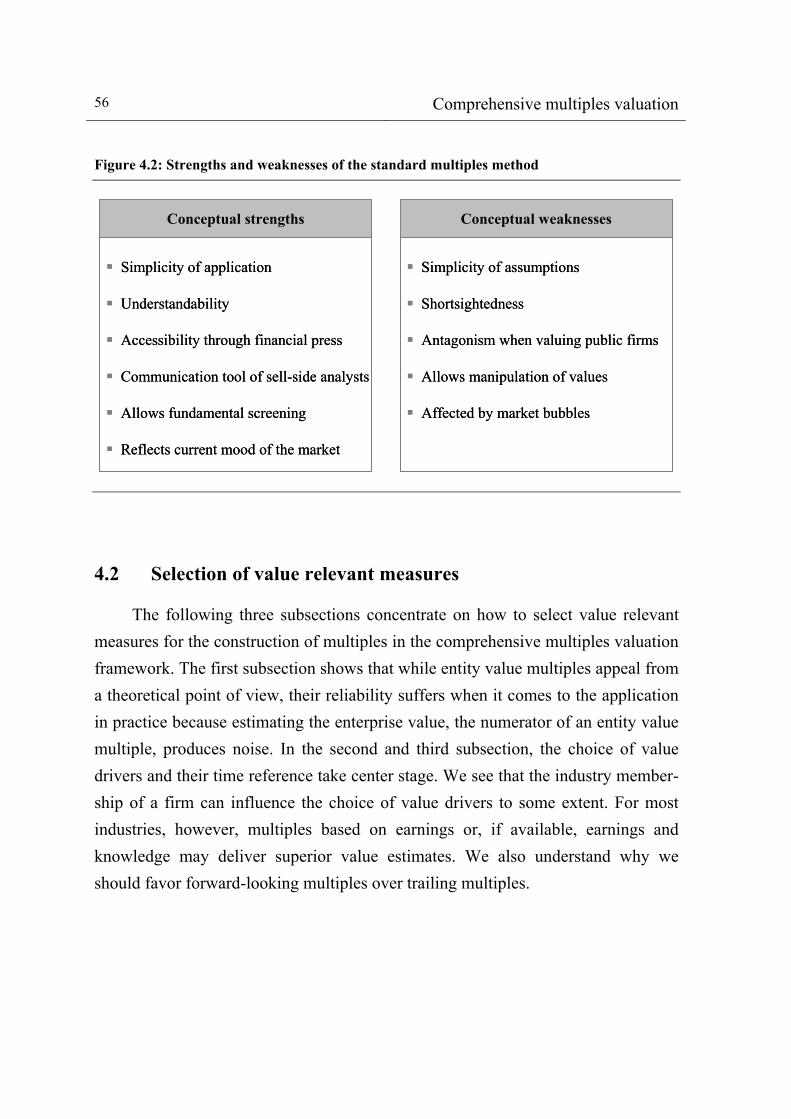
56 Comprehensive multiples valuation

Figure 4.2: Strengths and weaknesses of the standard multiples method

Simplicity of assumptions

Shortsightedness

Antagonism when valuing public firms

Allows manipulation of values

Affected by market bubbles

Conceptual weaknesses

Simplicity of application

Understandability

Accessibility through financial press

Communication tool of sell-side analysts

Allows fundamental screening

Reflects current mood of the market

Conceptual strengths

Simplicity of assumptions

Shortsightedness

Antagonism when valuing public firms

Allows manipulation of values

Affected by market bubbles

Conceptual weaknesses

Simplicity of application

Understandability

Accessibility through financial press

Communication tool of sell-side analysts

Allows fundamental screening

Reflects current mood of the market

Conceptual strengths

4.2 Selection of value relevant measures

The following three subsections concentrate on how to select value relevant measures for the construction of multiples in the comprehensive multiples valuation framework. The first subsection shows that while entity value multiples appeal from a theoretical point of view, their reliability suffers when it comes to the application in practice because estimating the enterprise value, the numerator of an entity value multiple, produces noise. In the second and third subsection, the choice of value drivers and their time reference take center stage. We see that the industry member-ship of a firm can influence the choice of value drivers to some extent. For most industries, however, multiples based on earnings or, if available, earnings and knowledge may deliver superior value estimates. We also understand why we should favor forward-looking multiples over trailing multiples.

Comprehensive multiples valuation 57

4.2.1 Equity value versus entity value multiples

4.2.1.1 Basic considerations. Many practitioners raise the question whether to use the market capitalization or the enterprise value (i.e., market capitalization plus book value of net debt) of a firm in the numerator of a multiple. From equation (3.30) and (3.31), we know that by using the market capitalization we receive equity value multiples, and by using the enterprise value, we receive entity value multi-ples. As their names suggest, the former yield direct estimates of a firm’s equity value when applied in the four-step valuation process, while the latter yield direct estimates of entity value – the equity value can be calculated indirectly by subtract-ing the target firm’s net debt from its entity value estimate.26

When working with entity value multiples, we also have to pay attention to preserve internal consistency by matching up the numerator with the denominator (Pereiro 2002, p. 254). That is, because the enterprise value in the numerator meas-ures the current value of the claims of both a firm’s debt holders and equity holders, entity value multiples should only utilize value drivers in the denominator, which are defined on an enterprise level. Potential value drivers include income statement items that are before interest payments, total assets and invested capital from the balance sheet, or measures of cash flow that exclude cash flows from financing ac-tivities (e.g., cash flow from operating activities or free cash flow).

In contrast, equity value multiples should be constructed using value drivers that are defined at an equity holder’s level. Possible value drivers are income state-ment items after interest payments to debt holders, book value of equity from the balance sheet, or dividends as a measure of cash flow. However, the matching prin-ciple for equity value multiples is frequently violated with the P/SA, P/EBIT(DA), or P/OCF multiple being accepted among practitioners.27 One reason for them to do so is that the application of equity value multiples spares them the time-consuming task of considering (net) debt in their valuations.

26 See equation (4.2) and (4.3). 27 The empirical study ignores the matching principle for equity value multiples to directly com-pare the empirical performance of equity value versus entity value multiples.

58 Comprehensive multiples valuation 4.2.1.2 Capital structure: a theoretical limitation of equity value multiples. In the-ory, however, the level of debt, or more precisely the capital structure, can create problems that decrease the reliability of valuations based on equity value multiples. In a Modigliani & Miller (1958) world without taxes, costs of financial distress, and other agency costs, different capital structures across firms affect equity value mul-tiples, if they are not defined on an equity holder’s level. As an illustration, let us assume we have an efficient market and two firms A and B, which are identical ex-cept for their capital structure. Firm A operates with a debt to equity ratio of two (i.e., two-thirds debt, one-third equity), whereas firm B operates with a debt to eq-uity ratio of one (i.e., half-debt, half-equity). Both firms have the same EBIT be-cause EBIT is before interest and therefore not affected by capital structure. Con-trariwise, firm A has a lower market capitalization (i.e., market value of equity) than firm B because it operates with more debt. Hence, firm A also has a lower P/EBIT multiple than firm B. Applying the multiples valuation framework, we would suggest firm A to be underpriced and firm B to be overpriced. But this con-clusion is wrong, because the market prices the equity of both firms correctly.

Remaining in the Modigliani & Miller (1958) world, managers have the op-portunity to artificially influence specific equity value multiples by swapping debt for equity and thereby adulterating the attractiveness of their firm to investors (Goedhart, Koller & Wessels 2005, p. 10). For instance, there is a systematic rela-tionship between the P/E multiple and leverage. To build this relationship, we start with a firm that operates entirely with equity. Clearly, the equity value equityv of such

a firm equals its entity value entityv and net income (NI) equals EBIT. Hence, the

unleveraged (intrinsic) P/E multiple /equityu uv NI equals the (intrinsic) EV/EBIT mul-

tiple /entityv EBIT

equity entityu

u

v vNI EBIT

= (4.4)

Comprehensive multiples valuation 59

In a second step, we allow the firm to also use debt financing. To measure the

level of net debt in the firm, we define leverage as the ratio of net debt to entity value

entity

Net debtLeveragev

= (4.5)

For the leveraged firm, net income equals EBIT less the interest payments to

the debt holders. The amount of interest payments equals the cost of debt net debtr times the amount of net debt, which we can receive by multiplying entity value

entityv by leverage

entity net debt

NI EBIT interest paymentsEBIT v leverage r

= −

= − ⋅ ⋅ (4.6)

Next, we rearrange equation (4.4) to substitute the entity value in equation

(4.6), and convert EBIT into a single term

1

equitynet debtu

u

equitynet debtu

u

vNI EBIT EBIT leverage rNI

vEBIT leverage rNI

= − ⋅ ⋅ ⋅

⎛ ⎞= ⋅ − ⋅ ⋅⎜ ⎟

⎝ ⎠

(4.7)

If we express the amount of net debt as the product of the entity value and lev-

erage, the equity value has to equal entity value times one minus leverage ( )1equity entityv v leverage= ⋅ − (4.8)

By rearranging equation (4.4) again and using equation (4.7) to eliminate

EBIT, we get

60 Comprehensive multiples valuation

( )

( )

1

1

1

equityequity u

u

equityu

equitynet debtuu

u

vv EBIT leverageNI

NI leveragevvNI leverage rNI

= ⋅ ⋅ −

⋅ −= ⋅

− ⋅ ⋅

(4.9)

Now, we are able to solve for the (intrinsic) P/E multiple of the leveraged firm

by dividing both sides of equation (4.9) by net income

( )

1

1

equityequityu

equityuu

net debtu

leveragevvvNI NI leverage rNI

−= ⋅

− ⋅ ⋅ (4.10)

At this point, we already see that the leveraged P/E multiple is a function of

the unleveraged P/E multiple, leverage, and the cost of debt. Leverage, however, appears in both the numerator and the denominator of equation (4.10), so it is diffi-cult to distinguish how leverage affects the P/E multiple. With a few algebraic transformations and substitutions, we can eliminate leverage in the numerator and eventually28

11

1

equityu

net debtequityu

equity net debtnet debtu

u

vNI rv

vNI rleverage rNI

−= +

− ⋅ ⋅ (4.11)

Equation (4.11) demonstrates three scenarios how managers can manipulate

P/E multiples with capital structure decisions. For firms whose unleveraged P/E multiple is larger than the reciprocal of the cost of debt, P/E multiples systemati-cally rise with leverage. Conversely, firms with an unleveraged P/E multiple over the cost of debt smaller than one, exhibit a drop in their P/E multiple as leverage

28 The derivation of the relationship between the P/E multiple and leverage is adopted from Koller, Goedhart & Wesseles (2005), p. 725-727.

Comprehensive multiples valuation 61

increases. If the unleveraged P/E multiple equals the cost of debt, leverage has no effect on the P/E multiple.

In a real world setting, taxes, costs of financial distress, and agency costs exist, shaping tradeoffs between debt and equity and making capital structure value rele-vant (Barclay & Smith 2005, p. 9). Modigliani & Miller (1963) show that under the existence of taxes, using debt instead of equity lowers tax payments and therefore creates value for shareholders because corporate tax laws allow firms to deduct in-terest payments, but not dividend payments. The tax benefits of higher leverage, referred to as tax shield from debt, are opposed by a greater probability of default and higher expected costs of financial distress. As a compensation for the increase in risk and the decrease in flexibility, shareholders demand a higher cost of equity and value decreases.29 The consideration of agency costs generally favors the use of debt over equity.30 If capital structure matters – as it is in reality – financing deci-sions have an influence on the value of a firm and therefore indirectly affect both equity value and entity value multiples (Coenenberg & Schultze 2002, p. 700-702). Entity value multiples are less affected because they are defined on an enterprise level (Suozzo, Cooper, Sutherland & Deng 2001, p. 25).

4.2.1.3 Noise in the estimation of enterprise value: a practical limitation of entity value multiples. On the other hand, the definition on an enterprise level induces a major problem of the applicability of entity value multiples. The problem arises be-cause – in contrast to the market capitalization, which is utilized in the construction of equity value multiples – we cannot observe the enterprise value of a firm in prac-tice. Instead, we have to settle for approximating the, usually not publicly available,

29 Highly leveraged firms face higher fixed interest payments than firms that operate with less debt and are, therefore, less flexible with respect to valuable investment opportunities (Myers 1977, p. 149). On the other hand, Jensen (1986) argues that a high debt to equity ratio prevents firms from overinvestment by limiting managers’ ability to invest free cash flow in unprofitable projects. 30 In this setting, agency costs are associated with the negative effects of insider information, which managers have about the value of their firm. The recognition of this information gap between man-agers and other market participants has led to the formulation of three related theories of capital structure decisions: market timing (Smith 1986), signaling (Ross 1977), and pecking order (Myers 1984).

62 Comprehensive multiples valuation market value of net debt with the book value of net debt.31 This approximation can produce considerable noise, especially in a changing interest rate and default risk market environment (Koller, Goedhart & Wessels 2005, p. 347).

Moreover, the composition and calculation of net debt in the balance sheet can vary significantly across firms, producing even more noise. Firms can operate with different kinds of debt (e.g., short-term versus long-term debt, senior versus subor-dinated debt, private versus public debt, non-convertible versus convertible debt) and levels of cash & equivalents. There may also be differences in the treatment of pension liabilities, employee stock options, or capitalized leases. In addition, some firms have preferred stock or off-balance sheet items such as operating leases and special purpose entities. Since the reconstruction of all (off-)balance sheet items is troublesome, we are better off accepting the published numbers and the associated noise in the estimation procedure of enterprise value.

Taken together, when comparing the features of equity value versus entity value multiples, the latter appeal in theory because they are less affected by capital structure. In contrast, equity value multiples can compensate for this theoretical drawback in practice because the market capitalization in the numerator can be di-rectly observed from market prices and therefore does not suffer from noise. Whichever multiple we prefer in a specific context, we should preserve internal consistency by defining both the numerator and the denominator at the same level of analysis.

4.2.2 Industry specific multiples

In the last subsection, we focused on the numerator of a multiple. Now we shift the attention to the denominator and the use of specific value drivers in differ-ent industries.32

4.2.2.1 Accrual flow multiples versus cash flow multiples. Fundamental valuation models tell us that the stream of discounted future payoffs determines the value of a

31 See equation (3.31). 32 For references to specific industries, I use the nomenclature provided by the ICB system.

Comprehensive multiples valuation 63

firm. These payoffs can come in the form of either cash flows or measures of (ab-normal) earnings. In line with the principles of value generation, a comprehensive multiples valuation framework has to consider either (derived forms of) accrual flow multiples or cash flow multiples, or both. Questions to be answered are, which multiple(s) to use in a specific context or industry, in which form, and why?

A comparison of the underlying value drivers of accrual flow multiples and cash flow multiples reveals that the former are a more promising choice because they tend to be more stable and easier to compare across firms. That is, the majority of firms practice earnings guidance, whereas investment and dividend policies, which affect the level of free cash flow and dividends – the most prominent meas-ures of cash flow – differ significantly across firms. Penman (2006) illustrates the problems of cash flow measures with the examples of Cisco Systems following a “no dividend” policy and General Electric reporting a negative free cash flow in each of the last five years. Consequently, cash flow multiples such as the P/D, EV/FCF, or EV/OCF multiple can only play a secondary role in the comprehensive multiples valuation framework.

Negative or low numbers, however, are not a unique problem of cash flow measures. Frequently, firms in young or cyclical industries have negative or only meager profits. In a situation where the target firm or several firms within the peer group make (net) losses, we cannot utilize the P/E multiple. Instead, we must move upwards in the income statement to detect an appropriate accrual flow measure. Of-ten, we can stop at EBIT or EBITDA, but sometimes, we have to move even further up to gross income or sales. The problem with moving towards the top number in the income statement is that with every step, we leave out valuable information. The EV/SA multiple completely ignores differences in the profitability across firms. The EV/GI multiple accounts for differences in the gross margin but still misses consid-erable information on the operating efficiency of firms. The EV/EBITDA multiple considers differences in the operating performance; it is a useful multiple as long as the capital intensity is relatively stable across the comparables. If this is not the case, the EV/EBIT multiple is the “first choice” accrual flow entity value multiple.

Reasonable choices for accrual flow equity value multiples are the price to pre-tax income (P/EBT) and the P/E multiple. The decision whether to use the one

64 Comprehensive multiples valuation or the other depends on the composition of the peer group. In general, we may pre-fer the P/E multiple because it incorporates the opportunity to add value through smart tax management. If we work with an international peer group, where firms face different corporate tax laws, we are better off using the P/EBT multiple.

4.2.2.2 The use of book value multiples in capital-intensive industries. Somehow, measures of accrual flow and thereof derived multiples always appear in the com-prehensive multiples valuation framework. In addition, the balance sheet can pro-vide additional information on a firm’s value, which measures of accrual flow do not capture (Burgstahler 1998, p. 327). Therefore, we also consider incorporating a book value multiple into the model, especially when valuing firms in capital-intensive industries – oil & gas, basic materials, industrials, utilities, and financials – where tangible (financial) assets are the key to value generation. Book value mul-tiples that come into question are the P/B multiple on an equity level as well as the EV/IC and the EV/TA multiple on an enterprise level. Invested capital includes the same items as enterprise value, but on a book value basis rather than a market value basis. Hence, invested capital only measures value creating (operating) assets, whereas total assets also include cash & equivalents, which create zero net present value. When comparing firms, only assets with the ability to create value are of in-terest. Therefore, the EV/IC multiple is a superior multiple compared to EV/TA multiple.

In general, the usefulness of book value multiples to gauge the value of firms relates to which extent book values can provide a reasonable estimate of the re-placement value (i.e., the hypothetical market value) of assets in place (Arzac 2005, p. 65). Firms in the financial industry (e.g., banks, (re)insurers, other investment firms) and the oil & gas industry (in particular oil & gas producers) face compre-hensive “mark-to-market” accounting regulations. For these firms, applying book value multiples makes sense. Conversely, most assets of basic material and indus-trial firms are based on historical costs, which frequently represent an inaccurate gauge of replacement values. In these industries, we have to reconsider using book value multiples by carefully weighing the pros and cons of information provided from the numbers in the balance sheet.

Comprehensive multiples valuation 65

4.2.2.3 The use of knowledge-related multiples in science-based industries. Throughout the last two decades, the corporate landscape has changed dramatically with the achievements and developments in information and internet technology. Today, the main source of value generation in many industries is knowledge. In other words, intangible assets and investments in R&D, rather than tangible assets, shape the growth and profitability of businesses and therewith determine future payoffs in science-based industries. Some people limit science-based industries to health care and technology, but I suggest a broader definition containing all indus-tries with a substantial exposure to intangible assets or R&D, or both of them. My definition contains oil & gas, basic materials, industrials, health care, telecommuni-cations, utilities, and technology. Firms within these industries typically have intan-gible assets on their balance sheet and invest in R&D to fuel the generation of fu-ture payoffs; at least the successful firms do so.

Conservative accounting standards force firms to aggressively amortize intan-gible assets and immediately expense R&D investments. Accounting conservatism does not only decrease the quality of reported earnings numbers, but also hampers the comparability across firms and eventually distorts valuation results. To avoid the negative effects of accounting conservatism in science-based industries, I advo-cate adding back amortization and/or R&D expenditures to earnings variables and working with knowledge-related multiples – EV/(EBIT+AIA), EV/(EBIT+R&D), EV/(EBIT+KC), P/(E+AIA), P/(E+R&D), P/(E+KC) – in the comprehensive multi-ples valuation framework.33

4.2.3 Time reference of value drivers

The last issue to be addressed for the choice of multiples is the time reference of value drivers. That is, the decision whether to use trailing multiples or forward-looking multiples. From a theoretical point of view, we should decide in favor of forward-looking multiples because they are consistent with the principles of valua-tion theory that the value of a firm equals the present value of future payoffs (Mox-ter 1983, p. 97-101).

33 For more details on accounting conservatism and knowledge-related multiples, see subsection 3.3.3.

66 Comprehensive multiples valuation

Empirical research underpins that forward-looking multiples are indeed more accurate predictors of value than trailing multiples. In particular, two studies attract high attention among academics as well as practitioners. In a sample of 142 U.S. IPOs, Kim & Ritter (1999) find that P/E multiples based on earnings forecasts for the subsequent two years outperform those based on historical earnings. As the analysis moves from trailing to one-year and to two-year ahead forward-looking multiples, the average valuation error decreases from more than fifty percent to 44 percent to 29 percent, respectively, and the percentage of firms valued within 15 percent of their actual stock price increases from 15 percent to 19 percent to 36 per-cent. Liu, Nissim & Thomas (2002a), in their broad investigation of U.S. equity markets, show a similar pattern. The median valuation error equals 23 percent for inverse P/E multiples based on historical earnings and falls to 18 percent and 16 percent when moving to one-year and two-year forward-looking multiples. The re-sults of the two studies are intuitively appealing because earnings forecasts should reflect future profitability and growth better than historical measures. Consistent with this reasoning, the performance increases by lengthening the forecast horizon from one year to two years.

Based on the principles of valuation and empirical evidence, I recommend us-ing forward-looking multiples whenever forecast data for the multiples we want to apply is available for the entire peer group. Since analysts’ practice is to make point in time estimates of earnings measures for only two years ahead, the most promis-ing choice are forward-looking multiples processing two-year ahead forecasts (Penman 2006, p. 51). Forecasts on a broad basis are typically available for EBIT(DA), pre-tax income, and net income. Unfortunately, forecasts for R&D ex-penditures and amortization of intangible assets are hardly available for all compa-rables, so we cannot construct forward-looking knowledge-related multiples.

4.2.4 Criteria for the selection of value relevant measures

The preceding three subsections presented pertinent issues for the selection of value relevant measures in the comprehensive multiples valuation framework. The following list is a summary of these issues and therewith constitutes the answer to research question 1:

Comprehensive multiples valuation 67

• Matching principle. Define the numerator and the denominator of a multiple

consistently.

• Capital structure. Different capital structures have a negative effect on the re-liability of the multiples valuation approach, in particular when working with equity value multiples.

• Noise. Entity value multiples involve the drawback that the market value of net debt is typically not observable and therefore must be approximated with the book value of net debt, which itself is tricky to measure.

• Earnings guidance and investment / payout policy. While earnings measures tend to be constant or constantly growing over time and across firms, meas-ures of cash flow are less stable because investment strategies and payout plans frequently differ across firms. Scaling market price variables by earnings measures is more promising than scaling them by measures of cash flow.

• Industry profitability. Firms in young or cyclical industries frequently report weak or even negative profits. To detect a suitable accrual flow multiple in such a situation, we must move upwards in the income statement towards sales. In profitable industries, bottom line income measures are more appro-priate because they incorporate more value relevant information.

• Composition of the peer group. An international peer group requires accrual flow multiples to be defined before taxes.

• Information content of book values. In the financial and the oil & gas industry where most assets enter the balance sheet as “marked-to-market,” book value multiples provide useful information on a firm’s value.

• Accounting conservatism. Conservative accounting standards reduce the qual-ity of earnings and hinder the comparability across firms in science-based in-dustries. Knowledge-related multiples mitigate these negative effects and thus constitute a practicable alternative to conventional accrual flow multiples.

• Incorporation of future prospects. Both theoretical consideration and empiri-cal evidence support the use of forward-looking multiples processing two-year analyst forecasts.

68 Comprehensive multiples valuation Figure 4.3: List of criteria for the selection of value relevant measures

Composition of the peer group

Information content of book values

Accounting conservatism

Incorporation of future prospects

Matching principle

Capital structure

Noise

Earnings guidance and investment / payout policy

Industry profitability

Criteria for the selection of value relevant measures

Composition of the peer group

Information content of book values

Accounting conservatism

Incorporation of future prospects

Matching principle

Capital structure

Noise

Earnings guidance and investment / payout policy

Industry profitability

Criteria for the selection of value relevant measures

4.3 Identification of comparable firms

After analyzing the selection criteria of value relevant measures for the con-struction of multiples, this section focuses on how to identify an appropriate peer group. That is, a basket of comparables with similar operating and financial charac-teristics. It starts with an evaluation of the usefulness of industry classification sys-tems and finds reasons in favor of working with professionally managed systems such as ICB industry codes. By assessing the components of industry classification systems in more detail, we learn that 3-digit and 4-digit industries adjusted for firms of different size and firms with operations in different regions are the most promis-ing choices for a peer group. Eventually, a peer group should consist of at least two, up to a maximum of ten, comparables.

Comprehensive multiples valuation 69

4.3.1 Industry classification systems

A cost efficient way to handle the challenging task of identifying the right firms for the peer group is to start by examining the target firm’s competitors or industry (Koller, Goedhart & Wessels 2005, p. 376-377). Sometimes, a firm lists its competitors in its annual report or on its webpage. If a firm does not disclose this information or if we prefer an independent alternative, we can use an industry clas-sification system. Today, many different systems exist but only three of them offer a broad coverage of firms and are widely accepted in research and practice: the Standard Industrial Classification (SIC), the Global Industry Classification Standard (GICS), and the Industry Classification Benchmark (ICB) system.34

Despite their well-documented problems by Guenther & Rosman (1994) and Kahle & Walkling (1996), most researchers use SIC codes to form industry parti-tions. Bhojraj, Lee & Oler (2003) suspect that the continuing popularity of SIC codes among researchers is attributable to the absence of superior alternatives. It can rather be traced back to the fact that SIC codes are available for free, in contrast to the proprietary GICS and ICB codes, which are often the first choice of analysts and investment bankers at big firms. In their empirical analysis, Bhojraj, Lee & Oler (2003) investigate the usefulness of four different industry classification systems in a variety of applications common in capital market research and provide evidence in favor of proprietary systems. Eberhart (2004) adds another five industry classifica-tion systems and shows that using Dow Jones industry codes – meanwhile re-branded into ICB codes – yield the highest valuation accuracy when valuing firms with the multiples valuation method.35

34 Beginning in 1997, the SIC system developed by the U.S. Census Bureau is in the process of being replaced by the North American Industry Classification System (NAICS) by the U.S. Census Bureau and the International Standard Industrial Classification (ISIC) by the United Nations. The Securities and Exchange Commission (SEC), however, still lists firms by SIC codes. The GICS system is jointly developed by Standard & Poor’s (S&P) and Morgan Stanley Capital International (MSCI). The ICB system is jointly developed by Dow Jones and the FTSE Group. 35 The results of Bhojraj, Lee & Oler (2003) and Eberhart (2004) make other studies, which com-pare the performance of alternative methods to detect comparables against SIC codes worthless. For the multiples valuation approach, those studies include Bhojraj & Lee (2002), Bhojraj, Lee & Ng (2003), and Herrmann & Richter (2003). All of these studies aim to identify peers based on underlying fundamental value drivers instead of industry groupings.

70 Comprehensive multiples valuation

The most compelling explanation for the superior performance of proprietary industry classification systems, in particular the GICS and the ICB system, is that those systems are professionally managed. The management includes regular re-views of the validity of firms’ industry codes and, if necessary, adequate adjust-ments. What is more, the industry groupings and subgroupings also get updated regularly to better reflect transformations in the industrial landscape. Conversely, firms’ SIC codes and SIC industry definitions are typically permanent (Pereiro 2002, p. 262). Since the identification of the peer group is a crucial success factor of any multiples valuation, we must try to get access to either GICS or ICB codes.36

In general, industry classification systems have a structure with several – mostly four – (sub)industry levels. For instance, the ICB system, which constitutes the system of choice in the empirical study, consists of ten industries, 18 supersec-tors, 39 sectors, and 104 subsectors (ICB 2004, p. 6-8). Every classified firm has a 4-digit industry code: the first number stands for the industry (1-digit code), the second number for the supersector within the industry (2-digit code), the third num-ber stands for the sector within the supersector (3-digit code), and the last number stands for the subsector within the sector (4-digit code).37

4.3.2 Assessment of comparability

A common belief among practitioners is that a large peer group results in ac-curate valuations because firm idiosyncrasies are more likely to cancel out (Palepu, Healy & Bernard 2000 ch. 11, p. 7). They use a broad industry definition such as 1-digit or 2-digit industry codes to identify comparables. By doing so, the synthetic peer group multiples are representative for a “typical” firm within the chosen indus-try, but they are only representative for the target firm, if the target firm is indeed a typical firm of the industry – unfortunately, this is usually not the case in reality. Actually, an enhanced method to identify comparables is to narrow the industry definition to 3-digit or even 4-digit codes. By nature, firms within a finer industry grouping are more similar with respect to their current operating characteristics. And, the more similar the comparables are to the firm being valued, the greater the

36 Academics should do the same for studies, in which they utilize industry groupings. 37 For more details, see Appendix A.

Comprehensive multiples valuation 71

degree of comparability and the more information they provide (Eberhart 2001, p. 1392).

With the collection of a list of firms with a similar product and service mix as the target firm – however, the work is not done. Next, we have to control for differ-ences in the financial characteristics and determine under which circumstances we prefer a regional bounded or an international peer group. Thereby, the distinction between small and large firms can make significant contributions (Alford 1992, p. 107). In general, large firms are less risky because their international scope gives them better access to customers and produces recurring revenues. Furthermore, economies of scale and economies of scope provide potentials for cost savings. On the other hand, small firms often operate as niche players on a regional basis. Under the precondition of financial health and enough financing power, small firms have higher strategic flexibility and growth potential. The best technique to determine firms of the same size is to build a size ranking, which is based on market capitali-zation or fundamentals such as sales or book values.

Since the number of large firms within a certain 3-digit or 4-digit industry is typically limited, we must use an international peer group. Thanks to the increasing convergence of accounting standards all over the world, interpretations of numbers in the financial statements across firms from different countries become more alike. Corporate tax laws, however, differ across countries, which forces us to apply mul-tiples defined before income taxes. Instead of the P/E multiple, for instance, we are better off with the P/EBT multiple when working with an international peer group. For small firms, I recommend choosing the peers from the same country or region for two reasons. First, the main competitors of small firms are typically other re-gional players. Second, even more important, small firms heavily depend on the economic situation of the region in which they operate. A firm in a booming region, for example, trades at higher multiples than the same firm would do in a region in an economic downturn.

Analysts and investors of small firms are often interested where a firm stands compared to the leading firms of an industry. To get an impression of the strategic position and to justify the valuation of a small firm, I propose to also analyze finan-cial ratios and multiples of an additional “hedging” peer group, which consists of

72 Comprehensive multiples valuation the industry leaders. The results obtained from the hedging peer group, however, only serve as a sanity check and as a mechanism to detect possibly mispriced indus-try niches.

A general advantage of identifying comparables on an industry basis is that firms within the same industry tend to have similar capital structures (Ross, Wester-field & Jaffe 2001, p. 451-452). This feature allows us to apply equity value multi-ples without concerns. With this insight, we may generally prefer using equity value multiples over entity value multiples because the former are not affected by noise.

4.3.3 Size of the peer group

Filtering firms for industry membership, size, and region increases the quality of comparability – however, the work is still not done. Depending on the specific situation, the filter process for industry membership, size, and region generates a certain number of potential peers. This number typically lies anywhere between zero and twenty firms. If we end up with fewer than two peers, we must either ease the restrictions or use another valuation method. If we have more than two peers, an examination of financial ratios and multiples of the remaining firms follows (Löh-nert & Böckmann 2005, p. 416). First, we check several financial ratios and exclude firms, which are not truly comparable to the target firm. After that, we examine the multiples. Sometimes, the peer group contains firms with negative or meager value drivers producing meaningless multiples. In such a situation, we must decide whether we eliminate only affected multiples or entire firms.

A final peer group of two to four firms is somewhat critical from a statistical point of view, but can be rational if the firms’ characteristics are almost identical or we include a hedging peer group into the valuation. Four to eight comparables is the ideal size for a peer group.38 More than ten peers can easily be misleading, espe-cially when we analyze a broad set of multiples (Pereiro 2002, p. 267). In such a case, I suggest to impose further restrictions to reduce the number of comparables.

38 This suggestion is derived from various conversations with academics, (hedge) fund managers, and investment bankers in Europe and the U.S.

Comprehensive multiples valuation 73

4.3.4 Criteria for the identification of comparable firms

The previous three subsections discuss important criteria for the identification of comparable firms in the comprehensive multiples valuation framework. As with the first research question, I provide an answer to research question 2 in form of a summary list of criteria: • Industry classification system. A professionally managed industry classifica-

tion system such as the GICS or the ICB system constitutes an ideal starting point for the identification of comparable firms.

• (Sub)industry level. Picking firms from a fine industry definition (i.e., 3-digit or 4-digit industry codes) produces a more homogenous group of potential peers than a broad industry grouping (i.e., 1-digit and 2-digit industry codes) can do.

• Size and region. The process of identifying the right peers continues with fil-tering for size. Using an international peer group is appropriate when valuing large caps. Conversely, for small caps, adding a regional filter makes sense.

• Hedging peer group. The use of a hedging peer group consisting of the indus-try leaders is a method to check the plausibility of a valuation obtained for a small firm and to detect possibly mispriced industry niches.

• Enhanced filter process. The examination of financial ratios and multiples of the remaining peer group candidates is the last step of the filter process. “Wrong” multiples or firms must be excluded.

• Number of comparables. Four to eight comparables is an ideal size for the peer group. Plus or minus two peers is still acceptable.

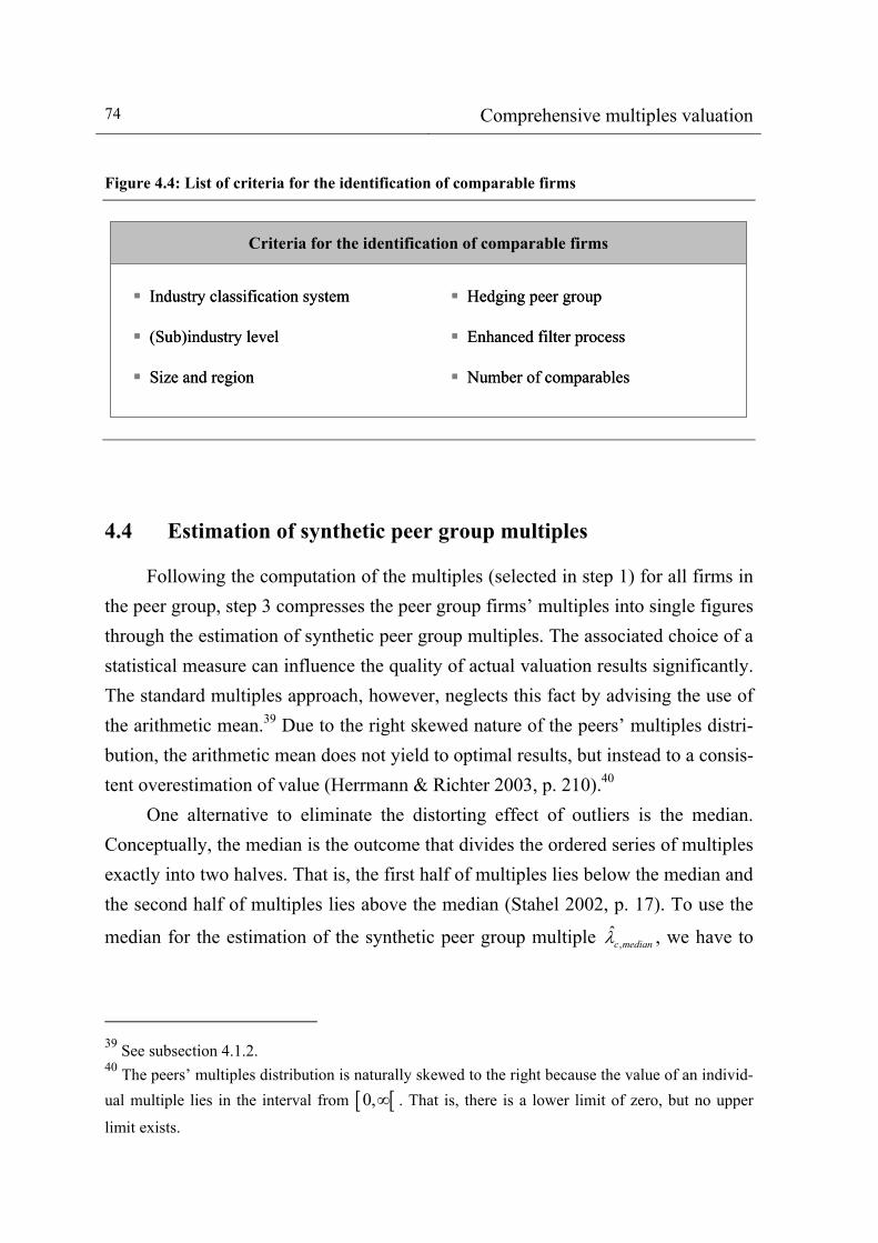
74 Comprehensive multiples valuation

Figure 4.4: List of criteria for the identification of comparable firms

Hedging peer group

Enhanced filter process

Number of comparables

Industry classification system

(Sub)industry level

Size and region

Criteria for the identification of comparable firms

Hedging peer group

Enhanced filter process

Number of comparables

Industry classification system

(Sub)industry level

Size and region

Criteria for the identification of comparable firms

4.4 Estimation of synthetic peer group multiples

Following the computation of the multiples (selected in step 1) for all firms in the peer group, step 3 compresses the peer group firms’ multiples into single figures through the estimation of synthetic peer group multiples. The associated choice of a statistical measure can influence the quality of actual valuation results significantly. The standard multiples approach, however, neglects this fact by advising the use of the arithmetic mean.39 Due to the right skewed nature of the peers’ multiples distri-bution, the arithmetic mean does not yield to optimal results, but instead to a consis-tent overestimation of value (Herrmann & Richter 2003, p. 210).40

One alternative to eliminate the distorting effect of outliers is the median. Conceptually, the median is the outcome that divides the ordered series of multiples exactly into two halves. That is, the first half of multiples lies below the median and the second half of multiples lies above the median (Stahel 2002, p. 17). To use the

median for the estimation of the synthetic peer group multiple ,c medianλ , we have to

39 See subsection 4.1.2. 40 The peers’ multiples distribution is naturally skewed to the right because the value of an individ-ual multiple lies in the interval from [ [0,∞ . That is, there is a lower limit of zero, but no upper

limit exists.

Comprehensive multiples valuation 75

rank the multiples 1 2, ,..., nλ λ λ of all firms 1,2,...,j n= of the peer group c into a size

adjusted list 1* 2* *, ,..., nλ λ λ and apply

( )

( )

* 1 / 2

,*/ 2 */ 2 1

= ˆ 1 =

2

n

c mediann n

if n odd

if n even

λλ

λ λ

+

+

⎧⎪= ⎨

⋅ +⎪⎩

(4.12)

The harmonic mean is another measure of central tendency, which is less sen-

sitive to outliers than the arithmetic mean (Fahrmeir, Künstler, Pigeot & Tutz 1999, p. 61-62). As a second appealing feature, the harmonic mean allocates equal weights to each firm in the peer group. To estimate a synthetic peer group multiple

,c h meanλ − based on the harmonic mean, we must build the inverse of the arithmetic

mean of the inverses of the multiples 1 2, ,..., nλ λ λ of all firms 1,2,...,j n= of the peer

group c

,

1

1ˆ1 1c h mean n

j jn

λ

λ

−

=

=⋅∑

(4.13)

Empirical results of Baker & Ruback (1999) and Herrmann & Richter (2003)

support the theoretical argumentation above. Both studies find that synthetic peer group multiples estimated using the median and the harmonic mean yield more ac-curate valuations than those based on the arithmetic mean or other measures of cen-tral tendency.41 When comparing the performance of the median and the harmonic

41 Other measures of central tendency are the mode, the (market) value weighted mean, or the loga-rithmic mean. All of these measures are affected by outliers and therefore a suboptimal choice for the estimation of synthetic peer group multiples. As an alternative to measures of central tendency, Damodaran (2001, 2002, and 2006) promotes using sector or market regressions to determine the value of the target firm instead of applying an estimated synthetic peer group multiple to the corre-sponding value driver of the target firm. The regression approach, however, fails in empirical tests (e.g., Herrmann 2002, p. 233 and unpublished results from the author of this book). This result does not surprise, since the theoretical link between multiples and the derived regression factors contradicts central assumptions of linear multi-factor regression models, such as no colinearity

76 Comprehensive multiples valuation mean, surprisingly, the former performs better in Herrmann & Richter (2003), whereas the latter performs better in Baker & Ruback (1999). Since the differences in performance are relatively small, both the median and the harmonic mean are suitable statistical measures for the estimation of synthetic peer group multiples. Typically, the median and the harmonic mean lie close to each other. However, they can vary considerably in a heterogeneous sample. For such situations, I recommend the construction of the average of (4.12) and (4.13) to determine an ultimate syn-

thetic peer group multiple cλ

, ,ˆ ˆ

ˆ2

c median c h meanc

λ λλ −+

= (4.14)

4.5 Actual valuation

No matter how carefully we identify comparable firms, the peer group’s oper-ating and financial characteristics are not perfectly identical to those of the target firm; the estimation of synthetic peer group multiples does not change this fact. Al-though the differences may be minor, making subjective adjustments is inevitable to ensure a trustworthy valuation. The adjustment process comprises an analysis of financial ratios and strategic advantages that explains variations in growth, profit-ability, and risk between the target firm and the peer group.

4.5.1 Ratio analysis

For the application in the comprehensive multiples valuation framework, ratio analysis involves comparing individual financial ratios and their development in recent periods between the target firm and its comparables. According to Palepu, Healy & Bernard (2000), we combine a cross-sectional analysis with a time-series analysis. The cross-sectional analysis (i.e., target firm versus peer group) helps to reveal operating and financial differences without tracking the ratios over time; it is only a rough snapshot, which can lead to wrong conclusions. Times-series analysis

between individual regression parameters or a normal distribution of regression residuals (Herrmann & Richter 2003, p. 214-215).

Comprehensive multiples valuation 77

identifies changes in financial performance and helps to see whether the most recent performance is unusual, in which case it should not be expected to recur in the fu-ture, or whether it is just one in a series of related outcomes.

Fortunately, ratio analysis enables the separate evaluation of the three key value drivers: growth, profitability, and risk, which reduces the complexity of allo-cating and consolidating performance differences. The analysis of growth is straightforward. As indicated in the discussion of fundamental equity valuation models and the derivation of intrinsic multiples in chapter 3, growth rates are com-monly reported for a variety of metrics, including sales, earnings, cash flows, divi-dends, assets, and common equity. Thereby, the growth in sales is the key long-term driver in all other metrics. Note that excess growth rates above the industry or the overall economy cannot sustain for long periods.

While the analysis of growth is straightforward, the analysis of profitability has numerous nuances. The starting and ultimate ending point is the return on common equity (ROCE). To understand the underlying sources of profitability, we have to decompose ROCE into its fundamental drivers (Palepu, Healy & Bernard, ch. 9, p. 4). For this purpose, the basic Dupont model or advanced versions of it can be helpful.42 The most common profitability ratios beside ROCE are: return on as-sets (ROA), return on invested capital (ROIC), gross (income) margin, EBIT(DA) margin, NOPAT margin, and net (income) margin.43

We know that costs of financial distress oppose the tax shield provided by us-ing debt instead of equity. In fact, leverage increases the riskiness of expected fu-ture cash flows because firms commit themselves to make fixed payments to credi-tors. The more debt a firm has, the greater the likelihood that unexpected losses will be amplified to the point where a firm cannot pay its creditors. In addition, even a firm with a respectable long-term potential can collapse, if it runs into short-term 42 In the formula of the basic Dupont model, ROCE equals net profit margin times asset turnover times total leverage: / / / / / /ROCE NI B NI TA TA B NI SA SA TA TA B= = ⋅ = ⋅ ⋅ . Advanced versions are presented in Palepu, Healy & Bernard (2000) chapter 9, Lundholm & Sloan (2004) chapter 5, and Penman (2004) chapter 11. Interested readers may also refer to Nissim & Penman (2001) who link (forecasted) growth and profitability ratios to equity valuation. 43 ROCE = net income / book value of common equity, ROA = net income / total assets, ROIC = NOPAT / invested capital, gross profit margin = gross income / sales, EBIT(DA) margin = EBIT(DA) / sales, NOPAT margin = NOPAT / sales, net (income) margin = net income / sales.

78 Comprehensive multiples valuation liquidity problems. Hence, the analysis of credit risk includes both an examination of a firm’s capital structure and the ability to meet short-term obligations (Lund-holm & Sloan 2004, p. 98). There are a number of ratios to evaluate the degree of risk arising from leverage: the debt to book value of common equity ratio, debt to market value of common equity ratio, and debt to total capital ratio are the most important leverage ratios.44 The current ratio, quick ratio, cash ratio, and EBIT(DA) interest coverage ratio are the prime liquidity ratios.45 In general, the computation of ratios for the peer group equals the estimation process of synthetic peer group mul-tiples. That is, we use the median, the harmonic mean, or a combination of both to aggregate financial ratios of comparables into a single ratio, which we then compare to the corresponding ratio of the target firm.

A careful ratio analysis makes a large contribution to the analysis of strategic advantages. In many cases, financial ratios can already clarify the differences be-tween the firm being valued and the peer group, so that an additional strategic analysis is probably not needed. If, however a lack of clarity remains, the applica-tion of strategic management tools such as the value chain concept, the five com-petitive forces analysis, the strengths, weaknesses, opportunities, and threats (SWOT) analysis, or the (New) St.Gallen Management Model can procure perspi-cuity.46

4.5.2 Adjustment factor

In the comparison of the target firm to the peer group, we should ultimately be able to answer questions such as: Does the target firm have higher growth rates, and if so how sustainable is the growth in the future? Is it gaining market share from

44 The most common measure of debt in ratio analysis is total debt, which equals short-term debt plus long-term debt (Smith, Ikenberry, Nayar, Anda, McVey & Stewart 2005, p. 40-45). Other variations can include total liabilities, net debt (total debt less cash & equivalents plus preferred stock), or solely long-term debt. Total capital equals total assets. 45 Current ratio = current assets / current liabilities, quick ratio = (cash & equivalents + accounts receivable) / current liabilities, cash ratio = cash & equivalents / current liabilities, EBIT(DA) interest coverage ratio = EBIT(DA) / interest expense. 46 To get an overview of these and many other strategic management tools, see Mintzberg, Lampel, Ahlstrand (1998) in English and Müller-Stewens & Lechner (2001) in German, or search for publi-cations at http://www.strategyclub.ch.

Comprehensive multiples valuation 79

rivals? Does the firm command a premium margin on its products? Is it producing and selling its products and services efficiently? Does it aggressively use leverage, and if so how does it handle the rising credit risk? Is it a market leader with out-standing products and services, a better access to customers, and an international scope? If these advantages (disadvantages) translate to a superior (inferior) growth, profitability, and risk profile, the target firm should trade at higher (lower) value.

Unfortunately, such a premium (discount) for differences in operating and fi-nancial characteristics is not reflected in valuation formula (4.2) or (4.3) of the standard multiples valuation method. To correct for this deficiency, I introduce an adjustment factor ,i tα so that formula (4.2) and (4.3) become47

, , , ,ˆˆ equity equity

i t i t c t i tp xα λ= ⋅ ⋅ (4.15)

( ) , , , , ,

ˆˆ ˆequity entity net debti t i t c t i t i tp x pα λ= ⋅ ⋅ − (4.16)

The adjustment factor ,i tα accounts for the accumulated value relevant differ-

ences in growth, profitability, and risk between the target firm and its comparables. It is a subjective variable that can lie anywhere within the interval of

[ ], 0.70 , 1.30i tα ≈ . For most firms and under the presumption of a comprehensive

process for the identification of the peer group, the adjustment factor should not exceed the range of [ ], 0.90 , 1.10i tα ≈ . Regularly, individual differences in the key

value drivers compensate each other to a total difference of zero and , 1i tα = . Using

an adjustment factor outside of the proposed range (i.e., ,0.70 1.30i tα> > ) is critical

and always requires explanation. Nevertheless, in rare cases, individual firms do more than thirty percent better or worse than their closest peers do. In particular, this is the case for “special” firms within an industry such as (quasi) monopolists or bankruptcy candidates.48

47 All other parameters of formula (4.2) and (4.3) remain the same. 48 The range for the adjustment factor, which I present here, functions for purposes of buying and selling limited proportions of stock. However, it is not representative for the valuation of corporate

80 Comprehensive multiples valuation

4.6 Two-factor multiples valuation model

4.6.1 Decision relevant multiples and hedging multiples

When valuing a firm using multiples, we can theoretically calculate a huge number of different multiples and analyze them. This procedure, however, does not make sense in practice, and indeed analysts and investment bankers restrict them-selves to a set of multiples – often, they apply five to eight multiples. By doing so, they get several valuations from which they typically take the average to estimate the equity value of the target firm. Besides the statistical drawback of the arithmetic mean, such an approach is also flawed because it mixes estimates of “good” multi-ples with those of “bad” multiples (Bonadurer 2003, p. 28-29).

To overcome this problem, we use the criteria for the selection of value rele-vant measures from section 4.2 and determine two categories of multiples. The first category consists of the best multiples in a specific valuation context. We refer to them as decision relevant multiples because they form the ultimate basis for our investment or transaction decisions. Any other multiple we calculate – depending on the preferences and availability of data these are five to eight multiples – falls into the second category. These multiples fulfill a similar purpose as the hedging peer group: that is, they serve as a plausibility check of the results obtained from the decision relevant multiples. Hence, we call them hedging multiples.

A closer look at the list of criteria reveals that only a limited number of multi-ples have the potential to qualify as decision relevant multiples. For most valuation settings, we are able to identify a single best or two best multiple(s). That is, we find a best multiple out of the universe of accrual flow multiples, cash flow multi-ples, alternative multiples, and forward-looking multiples:

transactions, where additional factors (e.g., M&A market cycle, estimated synergies, design and financing of the deal, taxes) have a significant impact on premiums for corporate control and con-sequently the value of ,i tα . See Brealy & Myers (2000) chapters 33 and 34, Ross, Westerfield &

Jaffe (2002) chapter 30, or Copeland, Weston & Shastri (2004) chapter 18 to get a basic under-standing of the impact factors on the value of corporate transactions.

Comprehensive multiples valuation 81

• Accrual flow multiples dominate cash flow multiples.

• If the target firm and its peers are profitable, multiples based on value drivers further down in the income statement dominate multiples based on value driv-ers at the top of the income statement.

• An international peer group requires multiples to be defined before taxes.

• Alternative multiples dominate traditional accrual flow multiples in science-based industries.

• And, if forecast data is available, two-year forward-looking multiples are the first choice.

Book value multiples must be treated separately since they are linked to the balance sheet and not to the income statement (Penman 1998, p. 294-295). In a situation where the balance sheet contains value relevant information, which the first decision relevant multiple misses, either the P/B or the EV/IC multiple serve as the second decision relevant multiple. This is particularly the case for firms in capi-tal-intensive industries that follow mark-to-market accounting rules.

The choice of equity value versus entity value multiples is tricky because it involves the tradeoff between capital structure and noise. The fact that firms from the same industry tend to operate at similar debt levels, gives equity value multiples an advantage. Whichever type of multiple we prefer in a specific context; we must follow the matching principle and be consistent in the definition of the numerator and the denominator.

4.6.2 Combination of two decision relevant multiples

The main message of the preceding paragraphs is that only the first best or the two first best multiple(s) constitute(s) the core of effective investment or transaction decisions; all other multiples act as controlling variables. Given the situation of a single best multiple, formula (4.15) or (4.16) yields one valuation result, which we can then verify by using hedging multiples. The case of two decision relevant mul-tiples imposes the problem that we get two, mostly different, valuation results and we are left with the question of how to combine them into one valuation. One op-tion is to simply take the average. By doing so, we put an equal weight on each de-

82 Comprehensive multiples valuation cision relevant multiples and implicitly assume their exclusive information content – value relevant information, which they do not have in common – to be equal. Cheng & McNamara (2000) utilize this assumption in their investigation of the valuation accuracy of single and combined P/E and P/B multiples in the U.S. equity market and find that the combined P/E-P/B model yields superior results. However, they also recognize that both the limitation to the P/E and P/B multiple and the use of equal weights are suboptimal and demand for further improvements.

So far, we developed a scheme for the selection of decision relevant multiples. In order to systematically combine the valuations of two decision relevant multi-ples, valuation formula (4.15) and (4.16), which we apply for single multiples, are extended to49

( ), , 1, , 1, , 1, , 2, , 2, , 2, ,ˆ ˆˆ equity equity equity

i t i t i t c t i t i t c t i tp x xα β λ β λ= ⋅ ⋅ ⋅ + ⋅ ⋅ (4.17)

( ) , , 1, , 1, , 1, , 2, , 2, , 2, , ,

ˆ ˆˆ ˆequity entity entity net debti t i t i t c t i t i t c t i t i tp x x pα β λ β λ= ⋅ ⋅ ⋅ + ⋅ ⋅ − (4.18)

The extended formula (4.17) for equity value multiples and (4.18) for entity

value multiples incorporate the value predictions of two decision relevant multiples

indicated by subscript 1 and 2: 1, , 1, , 2, , 2, ,ˆ ˆ, c t i t c t i tx xλ λ⋅ ⋅ . The corresponding weights for

each of the two multiples are 1, ,i tβ and 2, ,i tβ . To keep the model as realistic as possi-

ble, both weights have to be positive and their sum has to equal one; formally,

1, , 2, ,, 0i t i tβ β ≥ and 1, , 2, , 1i t i tβ β+ = . When we have two decision relevant multiples and

assign equal weights to each of them, then 1, , 2, , 0.5i t i tβ β= = . Obviously, formula

(4.17) and (4.18) also work for situations with a single decision relevant multiple:

1, , 1i tβ = and 2, , 2, , 2, ,ˆ, , i t c t i txβ λ do not exist.

Formula (4.17) and (4.18) gives us a two-factor multiples valuation model to allocate optimal weights on two decision relevant multiples wherewith we system-

49 Theoretically it is possible to combine two multiples of a different type (i.e., an equity value multiple together with an entity value multiple). However, such a combination does not make sense in practice because, in a specific context, we prefer either the one or the other type.

Comprehensive multiples valuation 83

atically combine the information content of the income statement and the balance sheet into one valuation. However, in the absence of empirical results any assign-ment of weights is pure guesswork. That is, we do not know how much weight to put on each decision relevant multiple when estimating the value of a specific firm. Without empirical evidence, the fifty-fifty weighting is the most suitable selection.

Taken together, my answer to research question 3 is neither a clear “yes” nor “no” but rather a diplomatic “it depends.” More precisely, whether the combination of information from book values and earnings into a two-factor multiples valuation model – formula (4.17) and (4.18) – is useful from a theoretical point of view or not, depends on the existence of an exclusive information content of book value multiples. Thereby, the information content itself depends on the industry member-ship and the exclusiveness of the information content, which is determined by its relation to the information content of the first decision relevant multiple. Also, note that since the first decision relevant multiple is not necessarily the P/E multiple, we cannot restrict earnings to net income; instead we must view earnings in a broader context, which incorporates any earnings related measures of accrual flow. Hence, only with reservations and under special circumstances, the two-factor multiples valuation model can be viewed as a reinterpretation of the RIV model.

5 Design of the empirical study

The conceptual framework, as developed in the preceding chapter, builds on the implications of finance and accounting theory and related empirical research. In order to undermine the comprehensiveness and to evaluate the practicability of the framework – in particular for European equity markets – I carry out an exclusive empirical study. The following section introduces the concept of value relevance, the cornerstone of the study. It also forms a link to market efficiency and explains the assumptions of the study. Next, I formulate hypotheses for research questions 4 to 10 and clarify the underlying methodology of the study. The presentation of the initial dataset and the discussion of descriptive statistics of the ultimate sample make up the final section in this chapter.

5.1 The concept of value relevance

5.1.1 Definition, interpretation, implementation

According to Barth, Beaver & Landsman (2001), value relevance research ex-amines the statistical association between accounting information (e.g., book val-ues, accrual flow measures, cash flow measures, and thereof derived constructs such as financial ratios and multiples) and equity market variables (typically stock prices or stock returns). Thereby, a stronger association is generally regarded as more de-sirable than a weaker association. This definition of value relevance, however, is vague and gives leeway to possible interpretations.

Under a valuation orientated interpretation, accounting information is value relevant if it contains or assists in predicting the variables used in fundamental eq-uity valuation models. Hence, the ability of the accounting information to predict future payoffs determines the value relevance of the information in question. In an-other interpretation, the statistical association measures whether market participants actually use the information in question in setting prices, so value relevance is measured by the ability of accounting information to change the total mix of infor-mation in the market. This implies that value relevant information changes stock prices (i.e., equity market values) because it causes market participants to revise

Design of the empirical study 85

their expectations. Under a third interpretation, the association between accounting information and market variables, particularly over a long horizon, indicates only that the accounting information in question is correlated with the information used by market participants. Taking this view, value relevance reflects the ability of ac-counting information to capture or summarize information, regardless of the source, that affects market values or stock returns. This interpretation – which is the one I use – does not require financial statements to be the initial source of information. It is consistent with the value relevance of financial statements stemming from either the content of the financial statements themselves or a settling-up role, in which financial statements discipline pertinent information such as knowledge-related variables or forecasts (Francis & Schipper 1999, p. 325-327).

In addition, Francis & Schipper (1999) present two ways of how to operation-alize a value relevance study. The first way is to concentrate on the total return, which could be earned from the foreknowledge of financial statement information. This approach has been applied in several contexts, starting with the Ball & Brown (1968) portfolio returns test of the information content of earnings announcements and Bernard & Thomas (1989 and 1990) testing market efficiency by examining whether the market’s reaction to good and bad news earnings announcements is quick and unbiased. The second way is based on the explanatory power of account-ing information for market value variables. That is, the ability of accounting meas-ures to explain equity market values or annual market-adjusted returns. The ex-planatory power approach follows directly from Lev’s (1989) discussion of the use-fulness of earnings measures to explain equity market variables and also finds fre-quent application in accounting capital market research (e.g., Easton & Harris (1991) or Collins, Maydew & Weiss (1997)).

Chang (1999) proposes a third form of implementation: the “goodness of fit” of a valuation model. That is, if value predictions based on a certain valuation model explain market values reasonably well, the value relevance of the model’s variables is thought to be relatively high.50 In other words, value relevance depends on the convergence of market value and intrinsic value, as estimated by the valua-

50 For the multiples valuation method, these variables include the value driver(s) of the multiple(s) in question of the target firm as well as the corresponding multiples of the comparable firms.

86 Design of the empirical study tion model (Pfeil 2004, p. 38). Frankel & Lee (1998), Dechow, Hutton & Sloan (1999), and Lee, Myers & Swaminathan (1999) popularize this approach in their studies on the valuation accuracy of the residual income valuation model. Since the multiples valuation method also directly uses accounting measures, it is best suited for this type of value relevance study. Therefore, I work with the goodness of fit approach in the empirical study.

5.1.2 The link between value relevance and market efficiency

Many researchers automatically associate value relevance research with the assumption of efficient capital markets. The clarification of this common belief ne-cessitates a clear understanding of the term market efficiency. To describe efficient capital markets, Copeland, Weston & Shastri (2004) contrast them, first of all, with perfect markets. They consider four conditions as necessary for perfect markets: (1) markets are frictionless (i.e., no transaction costs, taxes, or any kind of regulation, all assets are divisible and marketable); (2) there is perfect market competition (i.e., all market participants are price takers); (3) markets are informationally efficient (i.e., information is costless and received simultaneously by all market participants); and (4) all market participants are rational and maximize their expected utility.

Capital market efficiency is much less restrictive than the notion of perfect markets. In an efficient capital market, prices fully and instantaneously reflect all available and relevant information (Fama 1970, p. 383). Hence, we can relax the conditions of a perfect market outlined above. For instance, an efficient capital market still exists, if markets are not frictionless or if there is imperfect competition. Even biased or costly information and market participants’ irrationalities (e.g., overconfidence or underestimation, bubbles) do not contravene the existence of ef-ficient capital markets. Still, in a somewhat limited sense, efficient capital markets imply operational efficiency and prices, which are allocationally efficient (Cope-land, Weston & Shastri 2004, p. 354).

Fama (1970 and 1976) operationalizes the notion of what is today known as the efficient market hypothesis (EMH) by defining three forms of efficiency. Each form is based on a different view of what type of information is understood to be “relevant.” First, the weak form of capital market efficiency states that the market uses the history of prices and therefore market participants cannot earn excess re-

Design of the empirical study 87

turns by developing trading rules based on historical price patterns. Under the semistrong form of efficiency, prices fully incorporate any type of publicly avail-able information – hence, fundamental analysis becomes useless. Finally, the strong form of the EMH implies that prices reflect all available information including not publicly available insider information – earning superior returns is impossible. Fol-lowing both the evidence of many empirical studies in the finance and accounting literature, as well as the monitoring of market participants’ ability to generate ex-cess returns over a longer time window, capital markets can be viewed as efficient in the semistrong form – in particular equity markets in developed countries (Spre-mann 2006, p. 159).51

So after all, what is the link between value relevance research and market effi-ciency? In general, value relevance research only needs to assume that stock prices reflect market participants’ consensus beliefs. This definition does not require as-suming market efficiency. Thus, value relevance research does not need to assume that equity market values are “true” or unbiased measures of the unobservable in-trinsic value of firms’ equity (Barth, Beaver & Landsman 2001, p. 94-95). With the further assumption of market efficiency – at least in the semistrong form – the re-sulting inference relates to the extent to which the accounting information in ques-tion reflects the true underlying value.52

The kind of value relevance research utilized in the study is a measurement er-ror model. By assuming market efficiency, I set equity market values as benchmark and label them as “true.” By doing so, the multiples in question, which symbolize the accounting information, are measured with error relative to the benchmark. The multiples with the smallest measurement error are those with the highest valuation accuracy, and vice versa.53 Accordingly, a small valuation error is associated with high performance. Even without assuming market efficiency, the results of the em- 51 For a detailed overview of market efficiency event studies and cross-sectional tests of return predictability, see Fama (1991 and 1998), Kothari (2001), or Copeland, Weston & Shastri (2004) chapter 11. 52 Although the interpretation of results differs depending on whether market efficiency is assumed or not, there is no way to verify whether stock prices or accounting information utilized in a valua-tion model equal intrinsic values because intrinsic values are unobservable. 53 In the empirical study, I refer to the measurement error as valuation error. Some authors also use the term pricing error.

88 Design of the empirical study pirical study would have a practical impact, since they support determining “appro-priate” market values for privately held firms or subsidiaries of publicly traded firms. That is, applying multiples with high valuation accuracy gives an impression of how much the market is willing to pay for a certain firm. This is a particular in-terest of private equity and venture capital firms planning an exit or firms seeking an IPO.

5.2 Research hypotheses

The goal of the empirical study is to generate answers to research questions 4 to 10 introduced in the first chapter. After examining the theoretical foundations of multiples and advancing the standard multiples valuation method into a comprehen-sive framework for using multiples in practice, I can now formulate research hy-potheses to the empirical research questions. In course of the analysis of the empiri-cal study, I verify (i.e., validate or reject) these hypotheses and develop explicit an-swers to research questions 4 to 10. • Hypothesis to research question 4: Multiples approximate equity market val-

ues reasonably well. Different performance measures testify a high overall valuation accuracy of the multiples valuation method.

• Hypothesis to research question 5: Equity value multiples outperform entity value multiples.

• Hypothesis to research question 6: Knowledge-related multiples outperform traditional multiples in science-based industries.

• Hypothesis to research question 7: Forward-looking multiples outperform trailing multiples.

• Hypothesis to research question 8: A finer industry definition – smaller but more homogenous peer group – improves the valuation accuracy of multiples.

• Hypothesis to research question 9: The valuation accuracy of different multi-ples depends on the industry membership of the firm being valued.

Design of the empirical study 89

• Hypothesis to research question 10: Valuations which combine information

from book values and earnings into a two-factor multiples valuation model outperform valuations based on single multiples in a one-factor multiples valuation model, if book values incorporate exclusive information content over earnings.

Although the research hypotheses outlined above are not accompanied with commentaries, they are deemed logical and straightforward since they build on theoretical reasoning from earlier chapters. The first hypothesis is drawn from both the theoretical anchor, which intrinsic multiples have in fundamental equity valua-tion models (section 3.2), and existing empirical evidence on the valuation accuracy of fundamental and market-based valuation models (section 2.2). The hypotheses related to research questions 5 to 7 and 9 are derived from the criteria for the selec-tion of value relevant measures (section 4.2). The hypothesis to research question 8 is based on the criteria for the identification of comparable firms (section 4.3). Fi-nally, the hypothesis to research question 10 is drawn from the theoretical assess-ment of the two-factor multiples valuation model (section 4.6).

5.3 Research methodology

The verification of the seven research hypotheses is carried out step by step. First, I examine the performance of single multiples using the one-factor multiples valuation model.54 Then, I analyze the performance of combined multiples in the two-factor multiples valuation model and compare it to the performance of the one-factor model. To verify the hypotheses to research questions 4 to 8, I conduct a cross-sectional analysis. After that, I utilize an industry analysis for the investiga-tion of the remaining two research hypotheses.

54 The methodology used to evaluate the performance of single multiples is adopted partly from Alford (1992), Liu, Nissim & Thomas (2002a), and Herrmann & Richter (2003).

90 Design of the empirical study 5.3.1 Methodology using single multiples

In the first stage of the analysis, I follow the traditional one-factor multiples approach and require that the value of common equity ,

equityi tp of firm i in year t is

proportional to a specific value driver ,i tx of the firm

, , , ,ˆequity equity

i t c t i t i tp x eλ= ⋅ + (5.1)

, , , , ,

ˆ ˆequity entity net debti t c t i t i t i tp x p eλ= ⋅ − + (5.2)

where ,c tλ is the synthetic peer group multiple on the value driver, which is es-

timated on the basis of equivalent multiples observed for the comparable firms c within the peer group, and ,i te is the valuation error. When using entity value multi-

ples, we also must consider the value of net debt ,net debti tp of firm i and deduct it ac-

cordingly on the right hand side of equation (5.2) to get ,equityi tp . The valuation error

in equation (5.1) and (5.2) is unlikely to be independent of value because firms with higher values are likely to have larger absolute valuation errors. Baker & Ruback (1999) and Beatty, Riffe & Thompson (1999) show that the valuation error is ap-proximately proportional to the value. Therefore, scaling equation (5.1) and (5.2) by value should improve the efficiency of estimating the synthetic peer group multiple

, , ,

, ,

ˆ1

equityc t i t i t

equity equityi t i t

x ep p

λ ⋅+ = (5.3)

, , , ,

, ,

ˆ ˆ1

entity net debtc t i t i t i t

equity equityi t i t

x p ep p

λ ⋅ −+ = (5.4)

For the estimation of the synthetic peer group multiple ,c tλ , I impose the re-

striction that the expected scaled valuation error , ,/ equityi t i tE e p⎡ ⎤⎣ ⎦ is zero. By rearrang-

ing terms in equation (5.3) and (5.4), I can then estimate the synthetic multiple us-

Design of the empirical study 91

ing the median as an appropriate measure of central tendency.55 To obtain a predic-tion for the value ,ˆ equity

i tp of firm i, I multiply the estimator for the synthetic peer

group multiple ,c tλ by the equivalent value driver ,i tx of the firm being valued

, , ,ˆˆ equity equity

i t c t i tp xλ= ⋅ (5.5)

, , , ,

ˆˆ ˆequity entity net debti t c t i t i tp x pλ= ⋅ − (5.6)

I evaluate the valuation accuracy of the prediction by calculating scaled abso-

lute valuation errors

, , ,

, ,

ˆ equity equityi t i t i t

equity equityi t i t

e p pp p

−= (5.7)

To compare the performance of different multiples in terms of valuation accu-

racy, I examine measures of dispersion for the pooled distribution of scaled absolute

valuation errors , ,/ equityi t i te p . The key performance measures are the median absolute

valuation error and the fraction of absolute valuation errors below 15 percent of ob-served market values. By doing so, the results become more comparable to related studies, which focus on one of these measures to draw conclusions.56 Furthermore, the results should be less affected by irregularities since they are built on two, in-stead of one, key performance measures. To ensure reliability, I consider additional performance indicators such as the arithmetic mean, the standard deviation, quar-tiles ( 0.25q and 0.75q ), percentiles ( 0.10q and 0.90q ), and the fraction of absolute valua-

tion errors smaller than 25 percent.

55 Other alternatives would be the harmonic mean or a fifty-fifty combination of the median and the harmonic mean as proposed in section 4.4. I report numbers using the median because, for the underlying sample, the median delivered superior results compared to the alternatives. 56 In particular Kaplan & Ruback (1995 and 1996), Kim & Ritter (1999), Gilson, Hotchkiss & Ruback (2000), Lie & Lie (2002), Liu, Nissim & Thomas (2002a and 2005a), and Herrmann & Richter (2003).

92 Design of the empirical study

Characteristics of high performance in terms of valuation accuracy are on one hand small numbers for measures of central tendency (i.e., median, mean, quartiles, and percentiles) and the standard deviation, and on the other hand high numbers for the fractions of absolute valuation errors below 15 percent and 25 percent respec-tively. Any performance indicator is first calculated for each year. Then, the yearly numbers are aggregated using the average.

5.3.2 Methodology using combined multiples

For the second stage of the analysis, I relax the proportionality requirement and allow for a second multiple as explanatory variable in a two-factor multiples valuation model

, 1, , 1, , 1, , 2, , 2, , 2, , ,ˆ ˆequity equity equity

i t i t c t i t i t c t i t i tp x x eβ λ β λ= ⋅ ⋅ + ⋅ ⋅ + (5.8)

, 1, , 1, , 1, , 2, , 2, , 2, , , ,

ˆ ˆ ˆequity entity entity net debti t i t c t i t i t c t i t i t i tp x x p eβ λ β λ= ⋅ ⋅ + ⋅ ⋅ − + (5.9)

where ,ˆ equityi tp is the value of common equity of firm i in year t, 1, , 1, ,

ˆc t i txλ ⋅ and

2, , 2, ,ˆ

c t i txλ ⋅ are value predictions of two different multiples indicated by subscript 1

and 2, ,i te is the valuation error, 1, ,i tβ and 2, ,i tβ are the corresponding weights for

each multiple. These weights are assumed to be positive 1, , 2, ,, 0i t i tβ β ≥ and to add up

to one 1, , 2, , 1i t i tβ β+ = . Again, we have to subtract ,net debti tp , when working with entity

value multiples. As with the single multiples approach, I divide equation (5.8) and (5.9) by value to improve estimation efficiency and require that

1, , 1, , 1, , 2, , 2, , 2, , ,

, ,

ˆ ˆ1

equity equityi t c t i t i t c t i t i t

equity equityi t i t

x x ep p

β λ β λ⋅ ⋅ + ⋅ ⋅+ = (5.10)

1, , 1, , 1, , 2, , 2, , 2, , , ,

, ,

ˆ ˆ ˆ1

entity entity net debti t c t i t i t c t i t i t i t

equity equityi t i t

x x p ep p

β λ β λ⋅ ⋅ + ⋅ ⋅ −+ = (5.11)

Design of the empirical study 93

When estimating the synthetic peer group multiples 1, ,ˆ

c tλ and 2, ,ˆ

c tλ , the valua-

tion error is subject to the restriction that its expected value , ,/ equityi t i tE e p⎡ ⎤⎣ ⎦ is zero.

Based on the estimation of the synthetic multiples using the comparable firms’ me-dian multiples, we receive predictions for ,ˆ equity

i tp through

, 1, , 1, , 1, , 2, , 2, , 2, ,ˆ ˆˆ equity equity equity

i t i t c t i t i t c t i tp x xβ λ β λ= ⋅ ⋅ + ⋅ ⋅ (5.12)

, 1, , 1, , 1, , 2, , 2, , 2, , ,

ˆ ˆˆ ˆequity entity entity net debti t i t c t i t i t c t i t i tp x x pβ λ β λ= ⋅ ⋅ + ⋅ ⋅ − (5.13)

As with single multiples, I calculate scaled absolute valuation errors and even-

tually analyze measures of dispersion for the pooled distribution of absolute valua-

tion errors , ,/ equityi t i te p to examine the performance of valuations, which combine

information from book values and earnings into a two-factor multiples valuation model

, , ,

, ,

ˆ equity equityi t i t i t

equity equityi t i t

e p pp p

−= (5.14)

5.4 Data and sample

The underlying indices of the empirical study are the Dow Jones STOXX 600 and the S&P 500 index, which represent approximately 88 percent of the total mar-ket capitalization in Western Europe (Dow Jones 2006, p. 1) and 75 percent in the U.S. (Standard & Poor’s 2006, p. 1) respectively. Hence, they are reliable proxies for the total markets. So far, most studies test the valuation accuracy of the multi-ples valuation method with U.S. data. To overcome this bias, my study concentrates mainly on the European dataset. Nevertheless, the analysis of the U.S. dataset is useful for two reasons. First, it allows validating the results of the European data

94 Design of the empirical study and thus serves as an out-of-sample test. Second, it enables the comparison of the results with those of existing studies.57

The Dow Jones STOXX 600 index contains the 600 largest stocks traded on the major exchanges of 17 Western European countries.58 To classify firms into dif-ferent industries and subindustries, I use the ICB system. This industry classifica-tion system consists of four levels (in increasing fineness): ten industries, 18 super-sectors, 39 sectors, and 104 subsectors, and offers four-digit industry codes for all firms within the dataset.

To construct the data sample, I merge data from three sources: historical ac-counting numbers from the Worldscope database, market prices from the Data-stream database, and analyst forecasts from the I/B/E/S database. For the ten recent years from 1996 to 2005, I calculate up to fifty different multiples for each firm i in year t using accounting numbers and mean consensus analyst forecasts as of the beginning of January and market prices as of the beginning of April.59 I measure market prices four months after the fiscal year end to ensure that all year-end infor-mation is publicly available by then and is reflected in prices.

The sample considers data that satisfies the following criteria: (1) for individ-ual firms, there are no more than two types of stock (e.g., common stock and pre-ferred stock) traded at the domestic exchange and an unambiguous dataset is avail-able from the aforementioned sources;60 (2) for individual firm years, the market capitalization is above 200 million U.S. Dollar ($) and the value of net debt is posi-tive; (3) for individual multiples, the underlying value driver in the denominator of

57 All figures and tables presented for the European sample within the main text are shown for the U.S. sample in Appendix B. 58 The index universe is constructed by aggregating stocks traded on the major exchanges in Aus-tria, Belgium, Denmark, Finland, France, Germany, Greece, Ireland, Italy, Luxembourg, the Neth-erlands, Norway, Portugal, Spain, Sweden, Switzerland, and the United Kingdom. 59 I present results for all multiples shown in figure 3.2: Categorization of multiples except of the PEG multiple. As in related studies (e.g., Liu, Nissim, Thomas (2002a) or von Berenberg-Consbruch (2006)), the PEG delivers very weak results. For more details on the definition of vari-ables, see Appendix C. 60 I exclude firms, which are listed both as holding company and as subsidiary. In Europe, these firms include Fresenius (Medical Care) from Germany and Heineken, Reed Elsevier, and Unilever from the Netherlands. In the U.S., I exclude Dana Corporation, Scientific Atlanta, and Sovereign Bank because of ambiguous data.

Design of the empirical study 95

a multiple is positive, so that negative or infinite values are impossible; and (4) for the construction of the peer group and eventually for predicting equity values using multiples, I require the availability of at least seven comparables within the same industry definition. By doing so, statistical outliers cannot distort the empirical re-sults.61 In addition, the analysis is conducted out-of-sample, which means that the target firm is not part of the peer group.

Table 5.1: Sample characteristics and descriptive statistics

Panel A: Sample characteristics

Underlying index Dow Jones STOXX 600Regional coverage 17 developed countries in Western EuropeIndustry classification used Industry Classification BenchmarkStocks within the sample 592Period covered 10 years (1996-2005)

Panel B: Descriptive statistics of the sample

Median Mean 1stquartile

3rdquartile

Number ofobservations

Sales (mio $) 3558 9750 1223 9667 5367EBITDA (mio $) 577 1653 228 1511 4675EBIT (mio $) 410 1213 162 1065 4850Net income (mio $) 206 1144 86 535 4917

Total assets (mio $) 5830 38766 1974 19674 5373Invested capital (mio $) 3777 18494 1383 10814 4101Book value of equity (mio $) 1677 4284 661 4320 5255

Operating cash flow (mio $) 393 1364 152 1079 4178Cash dividend paid (mio $) 85 258 35 245 4662

Panel A presents the characteristics of the European sample. From the 600 stocks within the Dow Jones STOXX 600, eight stocks of four different firms (i.e., Fresenius (Medical Care), Heineken, Reed Elsevier, Unilever) are excluded because these firms are listed both as holding and as subsidi-ary, but only one set of accounting numbers is available for each year. Panel B presents the analysis results of the pooled sample of annual data from 1996 to 2005. Annual accounting numbers are as of the beginning of January each year. Negative numbers are excluded.

The resulting sample for the Dow Jones STOXX 600, which consists of 592

firms, is used for the descriptive statistics reported in panel B of table 5.1. The me-dian firm has annual sales of $3.56 billion, annual net income of $206 million, total

61 The minimum number of comparables criterion, does not apply in a real world application set-ting where a peer group of only two or three firms can be the best choice (see section 4.3).

96 Design of the empirical study assets of $5.83 billion, book value of common equity of $1.68 billion, and pays an annual dividend of $85 million. Thus, the median net profit margin and the median return on common equity equal 5.79 percent and 12.28 percent respectively. Firms also operate with considerable leverage at a debt to equity ratio of about two to one. However, note that all of the financial characteristics are heavily skewed to the right, as indicated by the large differences between the medians and the means. For most numbers the mean is even higher than the number for the third quartile.

To classify multiples into different types, I use a two-dimensional framework distinguishing in the first dimension equity value multiples from entity value multi-ples and in the second dimension accrual flow multiples, book value multiples, cash flow multiples, knowledge-related multiples, and forward-looking multiples. The construction of equity value multiples is straightforward. Entity value multiples are more complicated to construct because the market value of net debt is typically not publicly available. Following Kaplan & Ruback (1995) and Kim & Ritter (1999), the enterprise value of firm i equals its market capitalization plus its market value of net debt. As an approximation for the market value of net debt, which is typically not publicly available, I start with the book value of total debt add the book value of preferred stock and deduct cash & equivalents.

Table 5.2 presents summary statistics of the investigated equity value multi-ples. The median values of common equity value multiples are 16.8 for the P/E multiple, 2.1 for the P/B multiple, and 1.1 for the P/SA multiple. Reflecting ana-lysts’ overall expectations of positive future growth, in particular earnings growth, one-year forward-looking multiples are higher than the corresponding trailing mul-tiples but lower than the corresponding two-year forward-looking multiples. Inter-estingly, the median P/TA multiple is 0.6, whereas the median P/IC multiple is 1.0, which indicates that firms in Europe operate with a considerable high balance of cash & equivalents. This observation is especially evident for the second half of the time horizon of the study and represents a warning sign for value managers because cash & equivalents are non-value adding investments reducing the return on in-vested capital. Also, note that the number of observations is smaller for knowledge-related multiples and forward-looking multiples compared to traditional multiples. The former are restricted to science-based industries. Moreover, several national

Design of the empirical study 97

accounting regimes do not require firms to separately disclose their R&D and amor-tization expenditures in their income statement. The availability of forward-looking multiples is limited because the I/B/E/S database provides analyst forecasts only for the last six years of the study. Again, the distribution of multiples is positively skewed.

Table 5.2: Equity value multiples summary statistics

Median Mean 1stquartile

3rdquartile

Number ofobservations

Accrual flow multiplesP / SA 1.1 5.4 0.6 2.2 4950P / GI 4.4 6.9 2.5 7.8 3878P / EBITDA 6.4 10.2 4.1 9.5 4317P / EBIT 8.9 15.6 6.0 13.6 4493P / EBT 11.5 18.4 8.0 17.1 4615P / E 16.8 37.6 11.7 25.7 4566Book value multiplesP / TA 0.6 1.2 0.3 1.2 4957P / IC 1.0 1.6 0.6 1.9 3810P / B 2.1 4.1 1.3 3.6 4865Cash flow multiplesP / OCF 9.5 17.4 5.6 16.3 3909P / D 41.5 81.4 26.8 70.4 4449Knowledge-related multiplesP / (EBIT+R&D) 7.1 9.8 4.7 10.7 1116P / (EBIT+AIA) 8.4 12.3 5.7 12.4 1973P / (EBIT+KC) 6.5 8.7 4.3 9.6 1029P / (E+R&D) 11.3 15.8 7.4 16.6 1073P / (E+AIA) 14.1 19.6 10.0 20.2 1898P / (E+KC) 9.9 13.3 6.6 14.5 988Forward-looking multiplesP / SA 1 1.2 13.8 0.6 2.6 3150P / SA 2 1.1 14.0 0.5 2.4 3146P / EBITDA 1 6.5 23.0 4.3 9.8 2995P / EBITDA 2 5.9 17.7 3.9 8.6 2995P / EBIT 1 9.2 17.2 6.4 13.4 2929P / EBIT 2 8.1 38.6 5.8 11.3 2945P / EBT 1 10.5 14.8 7.7 14.9 3058P / EBT 2 9.3 30.7 6.9 12.6 3128P / E 1 15.8 31.0 11.6 22.7 3056P / E 2 14.1 21.6 10.7 19.1 3125

Equ

ity v

alue

mul

tiple

s

Note: multiples are calculated for each firm i in year t using accounting numbers and mean consen-sus analyst forecasts as of the beginning of January and market prices as of the beginning of April. Criteria for the calculation of multiples and thus inclusion into the summary statistics are: (1) firm i is part of the sample; (2) the market capitalization of firm i is above 200 million U.S. Dollar and the value of net debt is positive in an individual year t; and (3) the underlying value driver x of an individual multiple λ of firm i in year t is positive.

6 Empirical results

The following chapter is divided into three parts. First, I carry out a cross-sectional analysis. Thereby, I identify comparable firms based on the ICB sector level – identical 3-digit industry codes. The only exceptions occur in subsection 6.1.3 where I evaluate the valuation accuracy of knowledge-related multiples in sci-ence-based industries (defined on the ICB supersector level) and in subsection 6.1.5 where the fineness of the industry definition itself is in question. In the second part, an analysis of five key industries (defined on the ICB supersector level) investigates the existence of industry-preferred multiples and the performance of single versus combined multiples in each industry. The chapter concludes with a validation of the empirical results for the European sample using the U.S. sample and a discussion of the limitations of the study.

6.1 Cross-sectional analysis

6.1.1 Absolute valuation accuracy

Performance indicators of absolute valuation accuracy for all equity value multiples within the European sample are reported in table 6.1. This table fulfills the purpose of presenting absolute numbers of valuation accuracy. When looking into the first column, we see that for 18 out of 27 investigated equity value multi-ples, the median absolute valuation error lies below thirty percent. In other words, half of the value predictions deliver results no more than thirty percent above or below the actual market value of common equity. Five multiples yield median abso-lute errors of less than 25 percent. Also, note that the median absolute errors range from 21.5 percent to 43.8 percent. This range is comparable to the 28.7 percent to 70.9 percent range Herrmann & Richter (2003) report in their study using six differ-ent multiples.

Presented in the second column from the right of table 6.1, the fraction of ab-solute valuation errors within 15 percent of observed market values varies from 22.4 percent to 40.0 percent. As a comparison, Lie & Lie (2002) report a variation between 22.5 percent and 35.1 percent using a list of ten different multiples for U.S.

Empirical results 99

equity data. The percentage of errors smaller than 15 percent lies above thirty per-cent for 19 multiples. That is, thirty percent or more value predictions deliver re-sults no more than 15 percent above or below the market capitalization of the target firm.

The highlighted fields in table 6.1 indicate the best performing multiples in each multiples category. Another aspect we already observe is that multiples based on value drivers closer to the bottom line of the income statement perform better than multiples based on value drivers further up in the income statement. This ob-servation is not restricted to accrual flow multiples, but also applies to knowledge-related and forward-looking multiples. For instance, averaging the relative perform-ance differences from the median error and the fraction below 15 percent reveals that the P/EBT multiple outperforms the P/SA multiple by 37.4 percent. The rela-tively weak performance of the P/E multiple compared to the P/EBT multiple does not surprise because corporate tax rates vary within Europe. Therefore, the compa-rability of net income across firms from different countries decreases. Comparing book values and earnings, the two most popular accounting value drivers, the study finds that multiples based on earnings clearly outperform those based on book val-ues. Throughout the cross-section, book value multiples as well as cash flow multi-ples disappoint in their ability to explain market values. The poor performance of cash flow multiples contradicts the belief voiced by some that cash flow measures are better than accrual flow measures in representing future payoffs.

Analyzing the numbers for the additional performance indicators shown in the remaining four columns of table 6.1 corroborates the findings using the key per-formance measures. Taken together, I generally attest high valuation accuracy to the multiples valuation method. Hence, my answer to research question 4 is that differ-ent measures of valuation accuracy approve the ability of the multiples valuation method to explain equity market values reasonably well. I also view this answer as a confirmation of the industry practice of using multiples as the standard equity valuation approach.

Although I do not directly compare the performance of the multiples approach to that of fundamental equity valuation models, indirect comparisons substantiate my conclusion. For instance, the results for the absolute valuation accuracy of vari-

100 Empirical results ous multiples are similar to those reported in Kaplan & Ruback (1995 and 1996), Gilson, Hotchkiss & Ruback (2000), and Liu, Nissim & Thomas (2002a). These studies contrast the performance of the multiples valuation method to either the DCF or the RIV model. Their findings allocate about the same degree of valuation accuracy to both market-based and fundamentals based equity valuation models.

Table 6.1: Absolute valuation accuracy of equity value multiples

Median Mean 1stquartile

3rdquartile

Fraction< 0.15

Fraction< 0.25

Accrual flow multiplesP / SA 0.4374 0.7478 0.1816 0.7656 0.2294 0.3395P / GI 0.4000 0.6979 0.1620 0.7178 0.2464 0.3611P / EBITDA 0.2954 0.5083 0.1224 0.5547 0.3118 0.4449P / EBIT 0.2872 0.4942 0.1184 0.5551 0.3213 0.4618P / EBT 0.2809 0.4801 0.1140 0.5508 0.3189 0.4650P / E 0.2925 0.4831 0.1123 0.5610 0.3094 0.4571Book value multiplesP / TA 0.3775 0.6696 0.1561 0.6715 0.2585 0.3818P / IC 0.3480 0.6609 0.1364 0.6393 0.2797 0.4038P / B 0.3729 0.5600 0.1570 0.6458 0.2566 0.3733Cash flow multiplesP / OCF 0.3365 0.7256 0.1310 0.6712 0.3028 0.4209P / D 0.3468 0.6255 0.1366 0.6466 0.2811 0.4005Knowledge-related multiplesP / (EBIT+R&D) 0.2735 0.4599 0.1101 0.5294 0.3362 0.4791P / (EBIT+AIA) 0.2714 0.4572 0.1129 0.5083 0.3310 0.4732P / (EBIT+KC) 0.2849 0.4732 0.1027 0.5214 0.3398 0.4756P / (E+R&D) 0.2736 0.4543 0.1171 0.5218 0.3261 0.4805P / (E+AIA) 0.2537 0.4445 0.1003 0.4957 0.3461 0.4903P / (E+KC) 0.2729 0.4512 0.1093 0.4989 0.3244 0.4623Forward-looking multiplesP / SA 1 0.4376 0.7069 0.1915 0.7339 0.2241 0.3304P / SA 2 0.4297 0.6853 0.1940 0.7107 0.2248 0.3302P / EBITDA 1 0.2813 0.5568 0.1186 0.5504 0.3188 0.4755P / EBITDA 2 0.2658 0.4798 0.1156 0.4981 0.3285 0.4893P / EBIT 1 0.2628 1.9712 0.1128 0.5256 0.3346 0.4924P / EBIT 2 0.2483 1.7225 0.0971 0.4537 0.3662 0.5222P / EBT 1 0.2403 0.4101 0.0988 0.4675 0.3621 0.5265P / EBT 2 0.2151 0.3348 0.0854 0.4119 0.4003 0.5580P / E 1 0.2441 0.3649 0.0909 0.4621 0.3609 0.5152P / E 2 0.2155 0.3168 0.0863 0.4121 0.3954 0.5635

Equ

ity v

alue

mul

tiple

s

Analysis of absolute valuation errors Fractions

Note: statistical measures of absolute valuation accuracy (median, mean, 1st and 3rd quartile) are based on scaled absolute valuation errors (see equation (5.7)). The fraction <0.15 (<0.25) measures the proportion of scaled absolute valuation errors below 15 percent (25 percent).

Empirical results 101

6.1.2 Equity value versus entity value multiples

Theory suggests favoring entity value over equity value multiples because they are less affected by different capital structures among comparable firms. In practice, however, the estimation procedure of the market value of net debt involves considerable noise. Therefore, we face a tradeoff between capital structure inde-pendence and noise when selecting appropriate multiples. In valuation practice, portfolio managers typically prefer using equity value multiples, whereas invest-ment bankers have a preference for entity value multiples; equity analysts use both types of multiples in their research reports.

Most prior studies cover only one of the two types of multiples and thus do not assess differences in the quality of value predictions. Those studies, which consider both types – Alford (1992) and Liu, Nissim & Thomas (2002) – find empirical evi-dence for the superiority of equity value multiples, but are unable to provide any rationale why such results might be observed. They simply conclude that adjusting for differences in leverage does not improve valuation accuracy.

Table 6.2 presents the results of the evaluation of equity value versus entity value multiples. To isolate the performance impact of the multiples selection to the market price variable used, I reduce the universe of multiples to those based on value drivers, which are defined on an enterprise level. This includes sales, gross income, R&D expenditures, amortization costs, EBIT(DA), and the equivalent fore-casts from the income statement, total assets and invested capital from the balance sheet, and cash flow from operating activities from the cash flow statement. Even though all of the value drivers are more appropriate for entity value multiples, the explanatory power of entity value multiples lacks in comparison to that of equity value multiples.

For the comparison, I calculate absolute and relative differences in the per-formance of equivalent multiples. When focusing on individual multiples, the EV/IC multiple is the only entity value multiple with a lower median absolute valuation error than the equivalent equity value multiple. Expressed in absolute numbers its median error is 1.49 percentage points lower than that of the P/IC mul-tiple; in relative terms, the difference in performance equals 4.28 percent. Although the results are a bit more friendly for the second key performance measure, equity

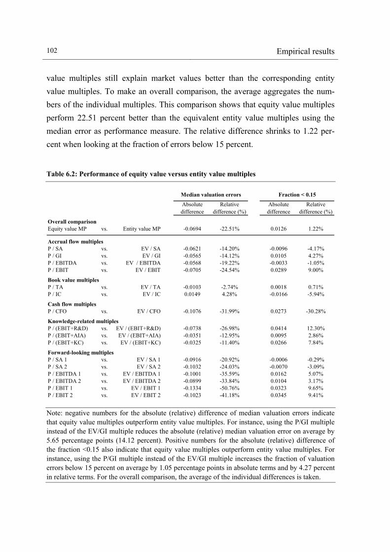
102 Empirical results value multiples still explain market values better than the corresponding entity value multiples. To make an overall comparison, the average aggregates the num-bers of the individual multiples. This comparison shows that equity value multiples perform 22.51 percent better than the equivalent entity value multiples using the median error as performance measure. The relative difference shrinks to 1.22 per-cent when looking at the fraction of errors below 15 percent.

Table 6.2: Performance of equity value versus entity value multiples

Absolutedifference

Relativedifference (%)

Absolutedifference

Relativedifference (%)

Overall comparisonEquity value MP vs. Entity value MP -0.0694 -22.51% 0.0126 1.22%

Accrual flow multiplesP / SA vs. EV / SA -0.0621 -14.20% -0.0096 -4.17%P / GI vs. EV / GI -0.0565 -14.12% 0.0105 4.27%P / EBITDA vs. EV / EBITDA -0.0568 -19.22% -0.0033 -1.05%P / EBIT vs. EV / EBIT -0.0705 -24.54% 0.0289 9.00%

Book value multiplesP / TA vs. EV / TA -0.0103 -2.74% 0.0018 0.71%P / IC vs. EV / IC 0.0149 4.28% -0.0166 -5.94%

Cash flow multiplesP / CFO vs. EV / CFO -0.1076 -31.99% 0.0273 -30.28%

Knowledge-related multiplesP / (EBIT+R&D) vs. EV / (EBIT+R&D) -0.0738 -26.98% 0.0414 12.30%P / (EBIT+AIA) vs. EV / (EBIT+AIA) -0.0351 -12.95% 0.0095 2.86%P / (EBIT+KC) vs. EV / (EBIT+KC) -0.0325 -11.40% 0.0266 7.84%

Forward-looking multiplesP / SA 1 vs. EV / SA 1 -0.0916 -20.92% -0.0006 -0.29%P / SA 2 vs. EV / SA 2 -0.1032 -24.03% -0.0070 -3.09%P / EBITDA 1 vs. EV / EBITDA 1 -0.1001 -35.59% 0.0162 5.07%P / EBITDA 2 vs. EV / EBITDA 2 -0.0899 -33.84% 0.0104 3.17%P / EBIT 1 vs. EV / EBIT 1 -0.1334 -50.76% 0.0323 9.65%P / EBIT 2 vs. EV / EBIT 2 -0.1023 -41.18% 0.0345 9.41%

Fraction < 0.15Median valuation errors

Note: negative numbers for the absolute (relative) difference of median valuation errors indicate that equity value multiples outperform entity value multiples. For instance, using the P/GI multiple instead of the EV/GI multiple reduces the absolute (relative) median valuation error on average by 5.65 percentage points (14.12 percent). Positive numbers for the absolute (relative) difference of the fraction <0.15 also indicate that equity value multiples outperform entity value multiples. For instance, using the P/GI multiple instead of the EV/GI multiple increases the fraction of valuation errors below 15 percent on average by 1.05 percentage points in absolute terms and by 4.27 percent in relative terms. For the overall comparison, the average of the individual differences is taken.

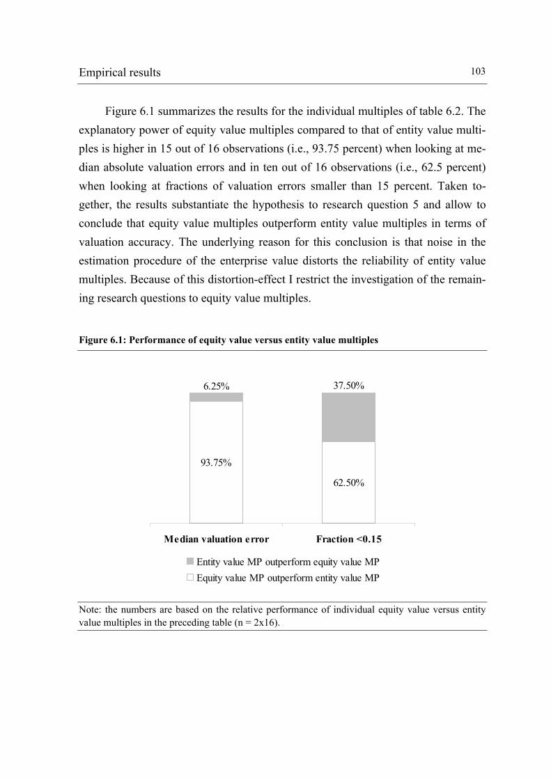
Empirical results 103

Figure 6.1 summarizes the results for the individual multiples of table 6.2. The

explanatory power of equity value multiples compared to that of entity value multi-ples is higher in 15 out of 16 observations (i.e., 93.75 percent) when looking at me-dian absolute valuation errors and in ten out of 16 observations (i.e., 62.5 percent) when looking at fractions of valuation errors smaller than 15 percent. Taken to-gether, the results substantiate the hypothesis to research question 5 and allow to conclude that equity value multiples outperform entity value multiples in terms of valuation accuracy. The underlying reason for this conclusion is that noise in the estimation procedure of the enterprise value distorts the reliability of entity value multiples. Because of this distortion-effect I restrict the investigation of the remain-ing research questions to equity value multiples.

Figure 6.1: Performance of equity value versus entity value multiples

93.75%

62.50%

6.25% 37.50%

Median valuation error Fraction <0.15

Entity value MP outperform equity value MPEquity value MP outperform entity value MP

Note: the numbers are based on the relative performance of individual equity value versus entity value multiples in the preceding table (n = 2x16).

104 Empirical results 6.1.3 Knowledge-related versus traditional multiples

Since the establishment of the personal computer in the early 1980s and the ensuing achievements in information and internet technology, knowledge has be-come the main source of value generation in many business areas. Today, the suc-cess of most firms within science-based industries such as oil & gas, basic materi-als, industrials, health care, telecommunications, utilities, and technology no longer relies on tangible assets, but rather on intangible assets and investments in R&D to create this type of assets. Due to the conservatism principle of accounting regimes, financial statements fail in properly reflecting the value of intellectual capital within firms. This proposition finds corroboration through several studies on the value relevance of intangibles and R&D investments.62 Although practitioners are aware of the impact, which knowledge can have on the value of a firm, knowledge-related variables do not find their way into market-based valuation so far.

In fact, valuations using accrual flow multiples frequently punish firms for op-erating with more intangibles or investing more in the creation of new intangibles through R&D than their peers. Such a dilution of value occurs because accounting rules mandate writing down intangible assets more aggressively than tangible assets and expensing R&D investments immediately in the financial statements. To over-come this problem induced by conservative accounting, I correct earnings-based accrual flow multiples for accounting costs of knowledge by adding back amortiza-tion, or R&D expenditures, or both of them (KC) to EBIT and net income. The emerging knowledge-related multiples are EV/(EBIT+R&D), EV/(EBIT+AIA), EV/(EBIT+KC), P/(EBIT+R&D), P/(EBIT+AIA), P/(EBIT+KC), and P/(E+R&D), P/(E+AIA), P/(E+KC).63

The performance of these multiples is evaluated on the ICB supersector level. Firms within twelve out of the 18 ICB supersectors exhibit a broad exposure to in-

62 E.g., Amir & Lev (1996), Lev & Sougiannis (1996), Aboody & Lev (1998 and 2000), Chan, Lakonishok & Sougiannis (2001), Lev & Thomas (2002), Pfeil (2003 and 2004), Eberhart, Max-well & Siddique (2004), Guo, Lev & Shi (2006), or Nelson (2006). 63 In practice, we can also add back AIA, R&D, or KC to other earnings based accrual flow meas-ures such as EBITDA or EBT. Theoretically, this procedure is also applicable to forward-looking multiples, if equivalent forecast data is available for the knowledge-related variables.

Empirical results 105

tangible assets and/or R&D.64 For those twelve supersectors, which I define as sci-ence-based industries, table 6.3 presents a comparison of the performance of knowledge-related versus traditional accrual flow multiples. The first two columns show numbers for the key performance measures of the study. Based on these num-bers, I compare the performance of individual multiples and construct performance rankings. First, I do this separately for each of the two multiple types (column 3 and 4) and then combined in a single ranking of all multiples (column 5 and 6). The separate analysis identifies the P/(E+R&D) and P/(E+KC) multiple as the best per-forming knowledge-related multiples. With a median absolute valuation error of 28.1 percent across the twelve supersectors, the P/(E+R&D) multiple ranks first followed by the P/(E+KC) multiple with a median error of 28.3 percent. The rank order changes, when looking at the fraction of valuation errors below 15 percent. Here, the P/(E+KC) multiple ranks first and the P/(E+R&D) multiple ranks second. In general, the variation in performance among the knowledge-related multiples is relatively small.

Another observation we can make in the separate rankings for both types of multiples is that performance improves by using value drivers closer to bottom line number in the income statement, suggesting that sales, gross income, and EBIT(DA) do not accurately reflect profitability by leaving out valuable informa-tion further down in the income statement.

The composite ranking in the last two columns of table 6.3 provides signifi-cant evidence for preferring knowledge-related multiples to traditional multiples in science-based industries. With the only exception of the EV/(EBIT+AIA) multiple for the second performance indicator, knowledge-related multiples deliver better value predictions than traditional multiples. More strikingly, the superiority is not restricted to the ranking itself, but also applies to the absolute numbers in the first two columns of table 6.3. Therefore, my answer to research question 6 is “yes,

64 The list of supersectors considerably exposed to either intangibles and/or R&D includes oil & gas (0500), chemicals (1300), basic resources (1700), construction & materials (2300), industrial goods & services (2700), automobiles & parts (3300), food & beverage (3500), personal & house-hold goods (3700), health care (4500), telecommunications (6500), utilities (7500), and technology (9500).

106 Empirical results knowledge-related multiples outperform traditional multiples in science-based in-dustries.”

Table 6.3: Performance of knowledge-related versus traditional multiples

Medianerror

Fraction< 0.15

Medianerror

Fraction< 0.15

Medianerror

Fraction< 0.15

Traditional accrual flow multiplesP / SA 0.4603 0.1995 6 6 12 12P / GI 0.4406 0.2111 5 5 11 11P / EBITDA 0.3280 0.2668 4 4 10 10P / EBIT 0.3100 0.2962 1 2 7 7P / EBT 0.3138 0.2989 3 1 9 6P / E 0.3129 0.2928 2 3 8 8

Knowledge-related multiplesP / (EBIT+R&D) 0.2980 0.3114 5 4 5 4P / (EBIT+AIA) 0.3018 0.2819 6 6 6 9P / (EBIT+KC) 0.2962 0.3135 3 3 3 3P / (E+R&D) 0.2807 0.3153 1 2 1 2P / (E+AIA) 0.2974 0.3077 4 5 4 5P / (E+KC) 0.2828 0.3252 2 1 2 1

Composite ranking of both multiple typesAbsolute performance

Rankings within thesame multiple type

Note: science based industries are identified on the ICB supersector level (2-digit codes) and in-clude oil & gas (0500), chemicals (1300), basic resources (1700), construction & materials (2300), industrial goods & services (2700), automobiles & parts (3300), food & beverage (3500), personal & household goods (3700), health care (4500), telecommunications (6500), utilities (7500), and technology (9500). The calculation of absolute performance numbers is limited to these twelve industries.

6.1.4 Forward-looking versus trailing multiples

Certainly, forward-looking multiples follow the principles of value generation. However, the important question is if multiples constructed on consensus analyst beliefs can also outperform when applied to empirical data. To tackle this problem, I compare the valuation accuracy of forward-looking multiples to that of the corre-sponding trailing accrual flow multiples. The comparison is carried out the same way as with the evaluation of equity value versus entity value multiples in subsec-tion 6.1.2. In fact, I compute absolute and relative differences in the performance of P/SA, P/EBIT(DA), P/EBT, and P/E multiples based on trailing numbers, one-year forecasts, and two-year forecasts.

Empirical results 107

Inspection of the overall comparison for differences in the median absolute

valuation error in table 6.4 shows that using one-year forecasts instead of trailing numbers decreases the median error on average by 2.54 percentage points, which is equal to 8.84 percent in relative terms (first row). Moving from one-year forecasts to two-year forecasts further improves valuation accuracy by 1.84 percentage points absolutely and 7.01 percent relatively (third row). Taken together, two-year for-ward-looking multiples outperform trailing multiples on average by 4.38 percentage points and 15.02 percent respectively (second row). By examining the results for the fraction of absolute valuation errors smaller than 15 percent, I find similar perform-ance improvements. This finding is consistent with what Kim & Ritter (1999) and Liu, Nissim & Thomas (2002) find in the context of U.S. IPOs and U.S. equities. It also supports Penman (2006) who promotes the incorporation of two-year forecasts into valuation models because two-year forecasts are equity analysts’ most powerful communication instrument in the perception of market participants.

A closer look at different multiples reveals an interesting pattern. In fact, the superiority of forecast information depends on the value driver used for the con-struction of multiples. The relative performance advantage utilizing forecasts of (pre-tax) earnings lies on average above 25 percent when comparing trailing num-bers and two-year forecasts. This advantage decreases significantly when switching to EBIT(DA) forecasts and eventually reverses into a relative disadvantage of fore-casts compared to historical figures for sales. To me, this pattern can be best ex-plained by the industry practice to determine an equity analyst’s quality (and pay-check) based on her ability to accurately forecast earnings. Therefore, analysts typi-cally devote their efforts towards the estimation of future earnings. In turn, the mar-ket also pays the highest attention to earnings forecasts and market values adjust accordingly.

108 Empirical results Table 6.4: Performance of forward-looking versus trailing multiples

Absolutedifference

Relativedifference (%)

Absolutedifference

Relativedifference (%)

Overall comparison1-year forecasts vs. Trailing numbers -0.0254 -8.84% 0.0219 6.85%2-year forecasts vs. Trailing numbers -0.0438 -15.02% 0.0449 14.13%2-year forecasts vs. 1-year forecasts -0.0184 -7.01% 0.0229 6.58%

SalesP / SA 1 vs. P / SA 0.0002 0.04% -0.0053 -2.31%P / SA 2 vs. P / SA -0.0077 -1.77% -0.0046 -2.01%P / SA 2 vs. P / SA 1 -0.0079 -1.81% 0.0007 0.30%

EBITDAP / EBITDA 1 vs. P / EBITDA -0.0141 -4.76% 0.0070 2.26%P / EBITDA 2 vs. P / EBITDA -0.0296 -10.02% 0.0167 5.36%P / EBITDA 2 vs. P / EBITDA 1 -0.0155 -5.52% 0.0097 3.03%

EBITP / EBIT 1 vs. P / EBIT -0.0244 -8.49% 0.0133 4.14%P / EBIT 2 vs. P / EBIT -0.0389 -13.54% 0.0449 13.96%P / EBIT 2 vs. P / EBIT 1 -0.0145 -5.52% 0.0316 9.43%

EBTP / EBT 1 vs. P / EBT -0.0406 -14.45% 0.0432 13.54%P / EBT 2 vs. P / EBT -0.0658 -23.42% 0.0814 25.53%P / EBT 2 vs. P / EBT 1 -0.0252 -10.49% 0.0382 10.56%

EarningsP / E 1 vs. P / E -0.0484 -16.53% 0.0515 16.63%P / E 2 vs. P / E -0.0770 -26.32% 0.0860 27.78%P / E 2 vs. P / E 1 -0.0286 -11.73% 0.0345 9.56%

Median valuation error Fraction < 0.15

Note: negative numbers for the absolute (relative) difference of median valuation errors indicate that forward-looking multiples outperform trailing multiples. For instance, using the P/E1 multiple instead of the P/E multiple reduces the absolute (relative) median valuation error on average by 4.84 percentage points (16.53 percent). Positive numbers for the absolute (relative) difference of the fraction <0.15 also indicate that forward-looking multiples outperform trailing multiples. For instance, using the P/E1 multiple instead of the P/E multiple increases the fraction of valuation errors below 15 percent on average by 5.15 percentage points in absolute terms and by 16.63 per-cent in relative terms. For the overall comparison, the average of the individual differences is taken.

To visualize the performance of forward-looking versus trailing multiples, fig-

ure 6.2 provides a bar chart containing the number of first, second, and third ranks of multiples based on trailing numbers, one-year forecasts, and two-year forecasts for pairwise performance evaluations on the ICB sector level. Out of 300 compari-sons, two-year forecasts perform best ranking first 160 times, second 108 times, and third only 32 times. One-year forecasts reach 72 first, 146 second, and 82 third

Empirical results 109

ranks. Far behind, trailing numbers rank first only 68 times, second 46 times, and third 186 times.

In sum, the results presented in table 6.4 and in figure 6.2 suggest the follow-ing ranking of multiples and therewith constitute the answer to research question 7. Forward-looking multiples, as a group, exhibit higher valuation accuracy than trail-ing multiples. This finding is intuitively appealing because earnings forecasts should reflect future profitability better than historical numbers. Consistent with this reasoning, performance increases with the forecast horizon from one year to two years.

Figure 6.2: Performance of forward-looking versus trailing multiples

1st 1st

2nd3rd

3rd3rd

1st2nd

2nd

Trailing numbers 1-year forecasts 2-year forecasts

Ran

king

s

1st 2nd 3rd

Note: the three bars indicate first, second, and third ranks of multiples based on trailing numbers, one-year forecasts, and two-year forecasts for pairwise performance evaluations (n = 300) on the ICB sector level (3-digit codes).

110 Empirical results 6.1.5 The effect of industry fineness

The identification of comparable firms has a crucial effect on the accuracy of the multiples valuation method. To conduct the analysis using comparable firms from the same industry, I considered alternative industry classification systems. Be-cause of the evidence that SIC codes frequently misclassify firms, I use the proprie-tary ICB system provided by Dow Jones and the FTSE Group.65 Another aspect that impacts valuation accuracy is the fineness of an industry definition used. This sub-section explores in detail the impact of identifying comparable firms based on dif-ferent levels of industry fineness. In the tests below, industry fineness, the number of ICB digits matched in selecting comparable firms, is varied between 1-digit (ICB industries), 2-digit (ICB supersectors), and 3-digit industry codes (ICB sectors). Visual examination of firms included in the same 4-digit industry (ICB subsectors) suggests it is too narrow to allow the inclusion of sufficient comparable firms given the loss of observations due to the requirement of a peer group size of at least seven firms.

In the first test, I again study absolute and relative performance differences. This time, it is a comparison of industry fineness levels for all five types of equity value multiples. Inspection of the overall comparison results in table 6.5 indicates that valuation accuracy improves significantly as the definition of an industry is narrowed from 1-digit over 2-digit to 3-digit codes. This finding is similar to what Alford (1992) finds for different levels of the SIC system. In contrast to his results, however, much of the improvement in the analysis occurs for matches on the third digit; the broader matches on the second digit show smaller effectiveness. Examin-ing median absolute valuation errors (fractions of valuation errors below 15 per-cent), the absolute and relative performance difference for 1-digit versus 2-digit codes are -2.1 percentage points (2.2 percentage points) and -6.3 percent (7.9 per-cent). The corresponding numbers for 2-digit versus 3-digit codes are -2.8 percent-age points (3.3 percentage points) and -8.7 percent (11.2 percent). Taken together, using ICB sectors (3-digit codes) instead of ICB industries (1-digit codes) results on average in 15.5 percent (18.3 percent) more accurate valuations. A perusal of the 65 E.g., Guenther & Rosman (1994), Kahle & Walkling (1996), Bhojraj, Lee & Oler (2003), or Eberhart (2004).

Empirical results 111

numbers in the remaining lines of table 6.5 supports the strengths of the overall findings, as it reveals the same performance pattern – without exception – through-out the individual multiple types.

Table 6.5: Performance of multiples depending on the industry fineness

Absolutedifference

Relativedifference (%)

Absolutedifference

Relativedifference (%)

Overall comparisonICB sectors vs. ICB supersectors -0.0280 -8.66% 0.0332 11.20%ICB sectors vs. ICB industries -0.0494 -15.48% 0.0547 18.26%ICB supersectors vs. ICB industries -0.0213 -6.30% 0.0215 7.93%

Accrual flow multiplesICB sectors vs. ICB supersectors -0.0263 -7.92% 0.0316 10.90%ICB sectors vs. ICB industries -0.0453 -13.64% 0.0470 16.24%ICB supersectors vs. ICB industries -0.0190 -5.30% 0.0155 5.99%

Book value multiplesICB sectors vs. ICB supersectors -0.0329 -8.98% 0.0372 14.05%ICB sectors vs. ICB industries -0.0618 -16.88% 0.0589 22.25%ICB supersectors vs. ICB industries -0.0289 -7.25% 0.0217 9.54%

Cash flow multiplesICB sectors vs. ICB supersectors -0.0405 -11.86% 0.0432 14.78%ICB sectors vs. ICB industries -0.0519 -15.20% 0.0589 20.18%ICB supersectors vs. ICB industries -0.0114 -2.99% 0.0158 6.33%

Knowledge-related multiplesICB sectors vs. ICB supersectors -0.0200 -7.37% 0.0239 7.17%ICB sectors vs. ICB industries -0.0484 -17.81% 0.0506 15.15%ICB supersectors vs. ICB industries -0.0284 -9.73% 0.0267 8.60%

Forward-looking multiplesICB sectors vs. ICB supersectors -0.0204 -7.18% 0.0302 9.12%ICB sectors vs. ICB industries -0.0394 -13.87% 0.0579 17.47%ICB supersectors vs. ICB industries -0.0190 -6.24% 0.0277 9.19%

Median valuation error Fraction < 0.15

Note: negative numbers for the absolute (relative) difference of median valuation errors indicate that a finer industry definition outperforms a broader industry definition. For instance, using the ICB sector (3-digit codes) definition instead of the ICB supersector (2-digit codes) definition for accrual flow multiples reduces the absolute (relative) median valuation error on average by 2.63 percentage points (7.92 percent). Positive numbers for the absolute (relative) difference of the frac-tion <0.15 also indicate that a finer industry definition outperforms a broader industry definition. For instance, using the ICB sector (3-digit codes) definition instead of the ICB supersector (2-digit codes) definition for accrual flow multiples increases the fraction of valuation errors below 15 per-cent on average by 3.16 percentage points in absolute terms and by 10.90 percent in relative terms. For the overall comparison, the average of the individual differences is taken.

112 Empirical results

The second test ranks 1-digit, 2-digit, and 3-digit industry codes based on pairwise performance evaluations of 27 equity value multiples. Figure 6.3 provides a graphical illustration on the dominance of ICB sectors over ICB supersectors and ICB industries. Out of 54 comparisons, 3-digit codes rank first 44 times, second four times, and third six times, followed by 2-digit codes reaching five first, 43 sec-ond, and six third places. Last, 1-digit codes rank first only five times, second seven times, and third 42 times.

While authors of standard valuation textbooks and most practitioners agree that comparable firms should be selected from the same industry, they do not indi-cate how an industry should be defined. The empirical results of the study suggest that forming a smaller but more homogenous peer group by narrowing the industry definition from 1-digit over 2-digit to 3-digit industry codes improves the valuation accuracy of the multiples valuation approach, and thus provide an explicit answer to research question 8.

Figure 6.3: Performance of multiples depending on the industry fineness

3rd

1st1st

1st

2nd

2nd

2nd

3rd 3rd

1-digit codes 2-digit codes 3-digit codes

Ran

king

s

1st 2nd 3rd

Note: the three bars indicate first, second, and third ranks of 1-digit, 2-digit, and 3-digit industry codes based on pairwise performance evaluations of 27 equity value multiples for both key per-formance indicators (n = 2x27).

Empirical results 113

6.2 Industry analysis

Given the focus on understanding the underlying information content of dif-ferent multiples and industry fineness definitions, the results, so far relate to cross-sectional data. To investigate the existence of industry-preferred multiples (research question 9) and the usefulness of a two-factor multiples valuation model (research question 10), I consider now industry specific data. The results are based on the five most important industries in Europe, as measured by the market capitalization of firms within the same ICB supersector. This includes oil & gas (0500), industrial goods & services (2700), health care (4500), telecommunications (6500), and banks (8300). Adding up the industry weights in table 6.6, reveals that the five key indus-tries account for more than the half (54.1 percent) of the total market capitalization of the Dow Jones STOXX 600. Banks with an industry weight of almost 22 percent are by far the most important industry in Western Europe.

Table 6.6: Dow Jones STOXX 600 industry weights

Code Name Weight Code Name Weight

0001 Oil & Gas 9.36% 0500 Oil & Gas 9.36%1000 Basic Materials 5.95% 1300 Chemicals 2.54%

1700 Basic Resources 3.41%2000 Industrials 9.19% 2300 Construction & Materials 2.44%

2700 Industrial Goods & Services 6.74%3000 Consumer Goods 11.32% 3300 Automobiles & Parts 2.12%

3500 Food & Beverage 5.14%3700 Personal & Household Goods 4.06%

4000 Health Care 9.15% 4500 Health Care 9.15%5000 Consumer Services 7.75% 5300 Retail 3.20%

5500 Media 2.93%5700 Travel & Leisure 1.63%

6000 Telecommunications 6.04% 6500 Telecommunications 6.84%7000 Utilities 5.97% 7500 Utilities 5.97%8000 Financials 31.58% 8300 Banks 21.95%

8500 Insurance 6.04%8700 Financial Services 2.79%

9000 Technology 3.68% 9500 Technology 3.68%

ICB industry1-digit codes

ICB supersector2-digit codes

Note: weights are calculated based on market data of the Dow Jones STOXX 600 as of February 15, 2006.

114 Empirical results 6.2.1 Industry-preferred multiples

The results of the cross-sectional analysis indicate that, among trailing multi-ples, equity value multiples outperform entity value multiples and knowledge-related multiples perform best in science-based industries. Further improvements can be made by the incorporation of forward-looking information based on consen-sus analysts’ forecasts. In addition, accrual flow measures closer to the bottom line number in the income statement constantly outperform measures further up in the income statement.

As financial and operational characteristics vary across industries, we might expect individual multiples to perform better in certain industries than in others. Theoretical coherence is presented in subsection 4.2.2 but can also be found in the literature.66 Furthermore, Tasker (1998) and Barker (1999a) derive empirical evi-dence from fairness opinions and surveys that practitioners indeed work with indus-try-preferred multiples. The usage of industry-preferred multiples, however, does not provide information about their ability to explain market values. To accurately test this ability, I construct two performance rankings for both key performance in-dicators within each of the selected European key industries. Since analyst forecast data is not available to many market participants, the first ranking is limited to trail-ing equity value multiples, whereas the second ranking further includes forward-looking equity value multiples.

For each ranking methodology, the first four columns of table 6.7 list the top-four performing multiples. In order to provide an insight into the numbers behind the rankings, the last two columns of table 6.7 also report the absolute valuation accuracy of the first-best and the fourth-best performing multiple. The highlighted fields indicate the most suitable choices of preferred multiples in each industry and ranking category. At first glance, we realize that for trailing multiples the general perception that different industries are associated with different best multiples holds. Including forecast data, however, refutes this perception as it reveals a clear dominance of two-year forward-looking earnings multiples, in particular the P/E2 multiple. In fact, the P/E2 multiple is part of the top-four across all industry rank- 66 E.g., Tasker (1998), Barker (1999a), Fernández (2002), Bonadurer (2003), Arzac (2005), Loderer (2005), Löhnert & Böckmann (2005), or von Berenberg-Consbruch (2006).

Empirical results 115

ings and, together with the P/EBT2 multiple, it ranks first in eight out of ten rank-ings. This pattern, which is consistent with the results in Kim & Ritter (1999) and Liu, Nissim & Thomas (2002a), suggests that the information contained in analysts’ two-year earnings forecasts captures a considerable proportion of value, and this feature is common to all industries.

Table 6.7: Industry-preferred multiples in European key industries

1st 2nd 3rd 4th 1st 4th

Oil & Gas Median pricing error P / B P / (E+R&D) P / IC P / (E+KC) 0.2569 0.2968Including forecasts P / E 2 P / B P / (E+R&D) P / EBITDA 2 0.2223 0.2720

Fraction < 0.15 P / IC P / B P / TA P / (E+R&D) 0.3363 0.3077Including forecasts P / IC P / E 2 P / B P / TA 0.3363 0.3094

Industrial Goods & Services Median pricing error P / (E+KC) P / (EBIT+KC) P / (E+AIA) P / (EBIT+R&D) 0.2709 0.3120Including forecasts P / EBT 2 P / E 2 P / EBIT 2 P / EBIT 1 0.2455 0.2724

Fraction < 0.15 P / (E+KC) P / (EBIT+AIA) P / EBT P / EBIT 0.2931 0.2654Including forecasts P / EBT 2 P / E 2 P / EBIT 2 P / EBIT 1 0.3296 0.2984

Health CareMedian pricing error P / (E+AIA) P / E P / (EBIT+AIA) P / OCF 0.2749 0.3489Including forecasts P / E 2 P / E 1 P / EBT 2 P / (E+AIA) 0.2328 0.2749

Fraction < 0.15 P / (E+AIA) P / E P / EBT P / (EBIT+AIA) 0.3521 0.2778Including forecasts P / (E+AIA) P / E 2 P / E 1 P / EBT 2 0.3521 0.3207

Telecommunications Median pricing error P / (EBIT+R&D) P / EBIT P / (EBIT+KC) P / OCF 0.2448 0.2955Including forecasts P / EBT 2 P / E 2 P / EBIT 2 P / EBT 1 0.1998 0.2339

Fraction < 0.15 P / OCF P / (EBIT+R&D) P / (EBIT+KC) P / EBIT 0.4118 0.3309Including forecasts P / EBT 2 P / OCF P / E 2 P / (EBIT+R&D) 0.4340 0.3673

Banks Median pricing error P / EBT P / E P / B P / D 0.2120 0.2828Including forecasts P / E 2 P / EBT 2 P / E 1 P / EBT 0.1621 0.2120

Fraction < 0.15 P / EBT P / E P / D P / B 0.3354 0.2670Including forecasts P / EBT 2 P / E 2 P / EBT 1 P / E 1 0.4846 0.3619

Best performing multiples Ranges

Note: performance rankings are constructed for both key performance indicators within five Euro-pean key industries. The first ranking is always limited to trailing equity value multiples; the sec-ond ranking also considers forward-looking equity value multiples. The first four columns list the four best performing multiples in each ranking category. The last two columns report the absolute performance of the best and fourth-best performing multiple in each ranking category.

116 Empirical results

Examination of absolute performances corroborates the finding that multiples approximate market values reasonably well. The median absolute valuation errors of the top performing multiples range from 16.2 percent (banks) to 27.5 percent (health care). The corresponding range for the fraction of valuation errors smaller than 15 percent goes from 48.5 percent (banks) to 29.3 percent (industrial goods & services). In general, multiples ranking first or second perform much better than those on the following two ranks do. On average, using the top multiple instead of the fourth-best multiple improves the performance by 17.5 percent. Also, note that except for banks, where multiples deliver outstanding valuation accuracy, the abso-lute level of valuation accuracy is surprisingly consistent across industries.

A closer look at industry-preferred trailing multiples encloses underlying eco-nomics and recent developments of different industries. Moreover, it helps to sense which value drivers are worthwhile to forecast in addition to earnings to construct superior multiples (e.g., knowledge-related forward-looking multiples) in a specific valuation context, and to eventually gain a competitive advantage.

Two observations from table 6.7 are of special interest. First, knowledge-related multiples, as a group, outperform traditional multiples in science-based in-dustries – this is nothing new. More interestingly, however, is the fact that the per-formance of knowledge-related multiples varies across industries. For instance, the P/(E+KC) multiple ranks first in industrial goods & services but does not appear within the top-three in either oil & gas, health care, or telecommunications. A simi-lar phenomenon applies to the P/(E+R&D) multiple in oil & gas, the P/(E+AIA) multiple in health care, and the P/(EBIT+R&D) multiple in telecommunications. How does this happen?

The usefulness of adding R&D expenditures and/or amortization of intangible assets to an earnings value driver depends largely on their consistency within an industry. The combination of both value drivers into the variable KC works best for industrial goods & service firms because these firms exhibit stable amortization costs and operate with constant annual R&D budgets. In contrast, R&D expendi-tures fluctuate in the health care industry because different stages in the new prod-uct development process require different levels of investment. During the last dec-ade, extraordinary M&A activity transformed the oil & gas and telecommunications

Empirical results 117

industry. This transformation process caused highly volatile amortization costs across firms because active acquirers accumulated huge amounts of intangible as-sets (including goodwill), which they started to amortize in subsequent years. Con-sequently, amortization of intangible assets should not be included in knowledge-related multiples when valuing oil & gas and telecommunications firms. In this con-text, also note that the higher performance of EBIT compared to net income in the telecommunications industry can be ascribed to several firms, which repeatedly re-ported net losses during the last ten years, particularly from 1996 to 1998 and again from 2001 to 2003.

The second observation we can make for trailing multiples in table 6.7 is that despite its weak performance within the cross-section, the P/B multiple ranks among the top-four in oil & gas and banks. This finding conforms to the notion that the effectiveness of book value multiples increases with the capital intensity of an industry and with the extent book values can provide a reasonable estimate of re-placement values. It also provides an indication of the P/B multiple’s ability to be incorporated in a two-factor multiples model for valuing oil & gas firms and banks.

As an answer to research question 9, this subsection finds evidence for the ex-istence of industry-preferred multiples for the restricted universe of trailing multi-ples. The inclusion of forward-looking multiples, however, reveals the dominance of the two-year forward-looking P/E multiple across all industries.

6.2.2 Single versus combined multiples

The usefulness of incorporating information from book value as a second de-cision relevant multiple into a two-factor multiples valuation model depends on: (1) its valuation accuracy in a specific industry; and (2) the exclusiveness of informa-tion provided over the first decision relevant multiple. Based on the results of the preceding subsection, the P/B multiple evidently fulfills the first condition in the oil & gas and the banking industry. Although not among the top-four multiples, the P/B multiple also performs reasonably in the health care industry.

The second condition can be best examined with an analysis of correlations. Table 6.8 presents the Pearson correlations for pairs of underlying value drivers of identified industry-preferred multiples. In general, value drivers are positively cor-related, which suggests that they share considerable information. The correlation

118 Empirical results coefficients among value drivers associated with the income statement (including forecasts) are remarkably high, at around ninety percent or more. Lower correla-tions can only be observed for operating cash flow and, in particular, book value of equity. The latter exhibits correlations below eighty percent with all other value drivers. This finding proves that some of the information content provided by book value multiples is exclusive and thus further supports the notion to systematically integrate the P/B multiple into a two-factor multiples valuation model.

Table 6.8: Correlations among selected value drivers

EBT E BV OCF EBT 2 E 2 EBIT+R&D E+R&D E+AIA E+KC

EBT 1.0000E 0.9737 1.0000BV 0.7285 0.7331 1.0000OCF 0.8766 0.8588 0.7678 1.0000EBT 2 0.9366 0.9183 0.7731 0.8851 1.0000E 2 0.9412 0.9518 0.7949 0.8900 0.9572 1.0000EBIT+R&D 0.9544 0.9443 0.7429 0.9188 0.9189 0.9416 1.0000E+R&D 0.8948 0.9302 0.7045 0.8460 0.8641 0.9178 0.9659 1.0000E+AIA 0.9598 0.9812 0.7579 0.9016 0.9166 0.9453 0.9526 0.9178 1.0000E+KC 0.8939 0.9248 0.7292 0.8841 0.8707 0.9190 0.9744 0.9883 0.9415 1.0000

Note: the correlation matrix shows Pearson correlation coefficients, which are calculated using the pairwise deletion method (n = 2326).

To test the valuation accuracy of the two-factor model, I combine the P/B mul-

tiple with the identified industry-preferred multiple in each of the five European key industries based on the methodology described in subsection 5.3.2. Thereby, I dis-tinguish again whether forecast data is available or not. For the determination of optimal weights, I minimize median absolute valuation errors. The optimization starts at the fifty-fifty weighting and is subject to the constraints that weights are positive and add up to one.67 The first and second two columns in table 6.9 summa-

67 Sensitivity analysis: using a non-intercept two-factor regression model yields comparable results with an adjusted R2 in the range between sixty and ninety percent. The factor coefficients (weights) are statistically significant on a five percent level, consistently positive, and approximately add up to one. However, since the theoretical link between multiples and the derived regression factors contradicts central assumptions of linear multi-factor regression models (e.g., no colinearity be-tween individual regression parameters and a normal distribution of regression residuals), the re-gression results are not presented.

Empirical results 119

rize the results of the optimization by reporting the underlying factors and the corre-sponding optimal weights.

Table 6.9: Factors and weights of the two-factor multiples valuation model in European key industries

Multiple 1 Multiple 2 Multiple 1 Multiple 2 Multiple 1 Multiple 2

Oil & GasExcluding forecasts P / (E+R&D) P / B 0.4014 0.5986 0.5000 0.5000

Including forecasts P / E 2 P / B 0.4968 0.5032 0.5000 0.5000

Industrial Goods & ServicesExcluding forecasts P / (E + KC) P / B 1.0000 0.0000 1.0000 0.0000

Including forecasts P / E 2 P / B 0.9782 0.0218 1.0000 0.0000

Health Care Excluding forecasts P / (E+AIA) P / B 0.8956 0.1044 0.9000 0.1000

Including forecasts P / E 2 P / B 0.8974 0.1026 0.9000 0.1000

Telecommunications Excluding forecasts P / (EBIT+R&D) P / B 0.9314 0.0686 1.0000 0.0000

Including forecasts P / E 2 P / B 1.0000 0.0000 1.0000 0.0000

Banks Excluding forecasts P / EBT P / B 0.5545 0.4455 0.5000 0.5000

Including forecasts P / E 2 P / B 0.8161 0.1839 0.9000 0.1000

Proposed weightsOptimal weightsFactors

Note: the first factor represents the identified industry-preferred multiple in each industry and cate-gory. Optimal weights are derived by minimizing median absolute valuation errors. The optimiza-tion starts at the fifty-fifty weighting and is subject to the constraints that the weights are positive and add up to one. The proposed weights are derived by personal judgment.

To convey the results into a general context and make them applicable for

practitioners, I use the optimal weights and thereof derive proposed weights for the two factors. Examination of the proposed weights in the last two columns of table 6.9 reveals that the P/B multiple indeed contains value relevant information in addi-tion to the first decision relevant multiple in the oil & gas, health care, and banking industry. In contrast, it does not have the ability to significantly improve the valua-tions obtained for industrial goods & service and telecommunications firms. The allocation of proposed weights is straightforward:

120 Empirical results • The simple fifty-fifty weighting works best for oil & gas firms and banks (if

forecasts are not available).

• A ninety-ten weighting (ten percent allocated to the P/B multiple) works best for health care firms and banks (if forecasts are available).

• Industrial goods & service and telecommunications firms are best valued using exclusively the best performing multiple in each industry.

The optimized model, by definition, delivers the most accurate valuations. However, the more interesting question is how much are these valuations actually better than the valuations obtained from the pragmatic model using proposed weights and the single multiples model? To tackle this problem, I compare absolute and relative differences of median absolute valuation errors between the three mod-els in the oil & gas, health care, and banking industry.

Table 6.10 reports the results of the comparison separately for two multiples universes: one excluding and the other including forward-looking multiples. Ex-amination of the results reveals two patterns. First, moving from optimal to pro-posed weights in the two-factor model has a negligible effect on performance. Ex-cept for the oil & gas industry excluding forecasts where the differences are higher, valuation accuracy declines on average only by 0.3 percentage points, which is equal to 1.77 percent in relative terms. The second pattern shows quite the opposite. In fact, comparing the proposed two-factor model with the single multiples model discloses significant differences in valuation accuracy. On average, the proposed two-factor model yields 9.9 percent more accurate valuations than single multiples. The difference is particularly evident for the industries and multiple categories where the fifty-fifty weighting is proposed.

Taken together, the results validate the hypothesis to research question 10 and let me conclude that valuations, which combine information from book values and earnings into a two-factor multiples valuation model, outperform valuations based solely on single multiples in industries where book values incorporate exclusive information content over the underlying value driver of the first decision relevant multiple. Within the analysis of European key industries, these industries are oil & gas, health care, and banks.

Empirical results 121

Table 6.10: Performance of single versus combined multiples in selected European key indus-tries

Absolutedifference

Relativedifference (%)

Absolutedifference

Relativedifference (%)

Oil & Gas 2 factor model / proposed vs. Proposed single MP -0.0572 -22.28% -0.0441 -19.85%2 factor model / optimal vs. Proposed single MP -0.0790 -30.74% -0.0447 -20.11%2 factor model / optimal vs. 2 factor model / proposed -0.0218 -10.89% -0.0006 -0.32%

Health Care 2 factor model / proposed vs. Proposed single MP -0.0181 -6.58% -0.0016 -0.69%2 factor model / optimal vs. Proposed single MP -0.0224 -8.15% -0.0038 -1.63%2 factor model / optimal vs. 2 factor model / proposed -0.0043 -1.67% -0.0022 -0.95%

Banks 2 factor model / proposed vs. Proposed single MP -0.0128 -6.04% -0.0065 -4.03%2 factor model / optimal vs. Proposed single MP -0.0150 -7.08% -0.0140 -8.62%2 factor model / optimal vs. 2 factor model / proposed -0.0022 -1.11% -0.0074 -4.79%

Including forecastsExcluding forecasts

Median absolute valuation errors

Note: negative numbers for the absolute (relative) difference of median valuation errors indicate that combined multiples outperform single multiples. For instance, using combined multiples in the two-factor model with proposed weights instead of proposed single multiples reduces the absolute (relative) median valuation error in the oil & gas industry on average by 5.72 percentage points (22.28 percent) when forecasts are excluded and by 4.41 percentage points (19.85 percent) when forecasts are included.

6.3 Evaluation of empirical results

6.3.1 Validation using U.S. data

The empirical results for the European sample substantiate the economics of the comprehensive multiples valuation framework. Nevertheless, before drawing general conclusions, it is worthwhile to validate the significance of the results using the U.S. dataset. The outcome of the validation, which can also be viewed as an out-of-sample test, surprises because it reveals not only comparable but also precisely equivalent results for all investigated research questions. In fact, even the magni-tude of many results shows high similarities. Appendix B presents the correspond-ing tables and figures.

122 Empirical results

Table 6.11: Comparison of absolute valuation accuracy in European and U.S. equity markets

Absolutedifference

Relativedifference (%)

Absolutedifference

Relativedifference (%)

Overall comparisonU.S. vs. Europe -0.0233 -10.01% 0.0345 8.87%

Accrual flow multiplesP / SA U.S. vs. Europe -0.0387 -9.72% 0.0262 10.24%P / GI U.S. vs. Europe -0.0498 -14.23% 0.0257 9.45%P / EBITDA U.S. vs. Europe -0.0022 -0.75% 0.0060 1.89%P / EBIT U.S. vs. Europe -0.0113 -4.09% 0.0143 4.25%P / EBT U.S. vs. Europe -0.0172 -6.52% 0.0324 9.23%P / E U.S. vs. Europe -0.0442 -17.78% 0.0490 13.66%

Book value multiplesP / TA U.S. vs. Europe 0.0174 4.40% 0.0009 0.36%P / IC U.S. vs. Europe 0.0303 8.01% -0.0089 -3.29%P / B U.S. vs. Europe -0.0593 -18.92% 0.0605 19.08%

Cash flow multiplesP / OCF U.S. vs. Europe -0.0139 -4.32% -0.0041 -1.38%P / D U.S. vs. Europe 0.0422 10.85% 0.0095 3.27%

Knowledge-related multiplesP / (EBIT+R&D) U.S. vs. Europe 0.0025 0.91% -0.0029 -0.88%P / (EBIT+AIA) U.S. vs. Europe -0.0077 -2.92% 0.0065 1.94%P / (EBIT+KC) U.S. vs. Europe -0.0116 -4.23% 0.0044 1.27%P / (E+R&D) U.S. vs. Europe -0.0111 -4.22% 0.0034 1.04%P / (E+AIA) U.S. vs. Europe -0.0162 -6.84% 0.0334 8.80%P / (E+KC) U.S. vs. Europe -0.0087 -3.30% -0.0026 -0.80%

Forward-looking multiplesP / SA 1 U.S. vs. Europe -0.0766 -21.21% 0.0501 18.28%P / SA 2 U.S. vs. Europe -0.0676 -18.68% 0.0401 15.12%P / EBITDA 1 U.S. vs. Europe -0.0274 -10.79% 0.0470 12.85%P / EBITDA 2 U.S. vs. Europe -0.0265 -11.09% 0.0726 18.10%P / EBIT 1 U.S. vs. Europe -0.0160 -6.47% 0.0538 13.85%P / EBIT 2 U.S. vs. Europe -0.0278 -12.58% 0.0520 12.44%P / EBT 1 U.S. vs. Europe -0.0134 -5.91% 0.0162 4.27%P / EBT 2 U.S. vs. Europe -0.0270 -14.34% 0.0391 8.90%P / E 1 U.S. vs. Europe -0.0732 -42.79% 0.1408 28.06%P / E 2 U.S. vs. Europe -0.0743 -52.64% 0.1665 29.64%

Median valuation error Fraction < 0.15

Note: negative numbers for the absolute (relative) difference of median valuation errors indicate that U.S. data yields more accurate valuations than European data. For instance, using U.S. data instead of European data for the P/SA multiple reduces the absolute (relative) median valuation error on average by 3.87 percentage points (9.72 percent). Positive numbers for the absolute (rela-tive) difference of the fraction <0.15 also indicate that U.S. data yields more accurate valuations than European data. For instance, using U.S. data instead of European data for the P/SA multiple increases the fraction of valuation errors below 15 percent on average by 2.62 percentage points in absolute terms and by 10.24 percent in relative terms. For the overall comparison, the average of the individual differences is taken.

Empirical results 123

One aspect of the results for the U.S. sample is of particular interest because it

provides supportive evidence for a phenomenon observed in prior research: ac-counting information exhibit greater value relevance in U.S. equity markets than elsewhere in the world (Ali & Hwang 2000, p. 20). Table 6.11 shows that across the universe of equity value multiples in the study, the median absolute valuation error (fraction of valuation errors below 15 percent) is on average 10.0 percent lower (8.9 percent higher) for the U.S. sample compared to the European sample. The most obvious explanation for the relative performance advantage of the U.S. sample is due to the heterogeneity of accounting and tax regulations in Europe. While U.S. firms are subject to both uniform accounting principles (U.S.-GAAP) and similar corporate tax rates, European firms face different accounting principles and tax rules.68 Mueller, Gernon & Meek (1994) offer an additional explanation by arguing that in market-orientated financial systems (i.e., the U.S.) the demand for published value relevant accounting information is higher than in bank-orientated systems (i.e., Europe with the exception of the UK) because banks typically have direct ac-cess to firm information. According to Herrmann & Richter (2003), the relative per-formance advantage of U.S. markets can also be due to a higher degree of capital market efficiency in the U.S.

Interestingly, much of the relative performance advantage reported in table 6.11 can be reduced to four multiples: the trailing P/E, the one-year forward-looking P/E, the two-year forward-looking P/E, and the P/B multiple. This finding indicates that: (1) the popularity of the P/E and the P/B multiple among U.S. market partici-pants has an impact on the market price levels of U.S. stocks; and (2) analysts cov-ering U.S. stocks produce earnings forecasts that better reflect intrinsic value gen-eration than analysts covering European stocks.

A closer look at the results of the cross-sectional analysis of the U.S. sample shows that entity value multiples perform slightly better in the U.S. than they do in Europe when compared to the equivalent equity value multiples. This amelioration, 68 European firms listed in the U.S. must provide financial statements based on U.S.-GAAP. Be-fore IFRS became mandatory for firms within the European Union (EU) by the end of fiscal year 2005, firms were allowed to report financial statements based on national accounting principles. This procedure is still feasible for firms in non-EU member countries, except for the majority of large caps. (Berndt 2005, p.12-31).

124 Empirical results however, lapses through the additional provision of equity value multiples consis-tent with the matching principle. Furthermore, the findings in favor of knowledge-related and forward-looking multiples compared to traditional and trailing multiples are stronger in the U.S. than in Europe. Conversely, the evidence supporting finer industry definitions is a bit weaker.

The industry compositions of the Dow Jones STOXX 600 and the S&P 500 index differ insofar that technology stocks play an eminent role in the U.S. econ-omy. In fact, they swamp telecommunications stocks out of the five key industries and supersede banks as the most important industry. Their industry-preferred trail-ing multiple is the P/(E+KC) multiple; including forecasts, the two-year forward-looking P/E multiple performs best. Moreover, the comparative analysis of the four remaining key industries yields exactly the same industry-preferred trailing multi-ples and approves the dominance of the two-year forward-looking P/E multiple across industries in both equity markets. Also, the results of the optimization and the derived proposed weights for the two-factor multiples valuation model are simi-lar – except for the oil & gas industry including forecasts where book values do not contain exclusive information content over two-year earnings forecasts.

6.3.2 Limitations

The preceding subsection presents evidence on the consistency of the empiri-cal results across different markets. Another frequently addressed issue for the as-sessment of empirical research quality concerns the time stability of the results. To evaluate the steadiness of the results, I focus on eleven representative equity value multiples and calculate calibrated performance indicators in each year from 1996 to 2005. In an aggregated form, figure 6.4 shows the progression of the calibrated me-dian absolute valuation errors and quartile errors for the European sample over the horizon of the study. The absolute and relative levels of those performance indica-tors appear fairly consistent over time. One noticeable deviation from this descrip-tion occurs during the years of the boom and bust of the dot-com bubble. That is, after a decline of valuation accuracy in 1999 and 2000, we observe a reversion in 2001 and further slightly positive adjustments in the years thereafter.69 Notwith-

69 This observation is particularly evident for the U.S. sample (see Appendix B).

Empirical results 125

standing this deviation, the flat curves in figure 6.4 suggest that the overall results are robust and observed consistently throughout the ten-year sample period.

Figure 6.4: Time stability of calibrated absolute valuation errors in Europe

0.00

0.25

0.50

0.75

1.00

1.25

1.50

1.75

2.00

2.25

1996 1997 1998 1999 2000 2001 2002 2003 2004 2005

Cal

ibra

ted

valu

atio

n er

ror

1st quartile Median absolute valuation error 3rd quartile

Note: to illustrate the time stability of valuation accuracy, calibrated performance indicators (me-dian absolute valuation error, 1st and 3rd quartile) are calculated in each year from 1996 to 2005 for eleven representative equity value multiples. The arithmetic mean is used for the aggregation of performance indicators.

The dataset and sample selection criteria, however, impose three notable limi-

tations on the empirical results. The first limitation concerns the selection of the Dow Jones STOXX 600 and S&P 500 as the underlying indices of the study. Al-though they cover the majority of the total market capitalization in Western Europe and the U.S., the number of stocks is limited to only 600 and 500 respectively. Classifying single stocks in large cap or mid cap, the sample entirely excludes small cap stocks. Furthermore, countries in Western Europe and the U.S. represent devel-

126 Empirical results oped equity markets as opposed to many countries in emerging markets. Therefore, it is questionable, if the results can be directly transferred to small caps and emerg-ing markets.

Limited data availability represents the second limitation. The dataset itself is unique because the access to resources of Thomson Financial in Zurich provides detailed I/B/E/S forecasts on many value drivers beyond the typically available earnings (growth) forecasts through academic resources. Complete forecast mate-rial, however, is still only available for the last six years from 2000 to 2005 for the European sample and for the last three years from 2003 to 2005 for the U.S. sample respectively. The analyses of forward-looking multiples are adjusted accordingly. Also, the dataset on R&D expenditures and amortization of intangible assets for firms in science-based industries is incomplete because of non-uniform disclosure regulations in different countries and industries. The two limitations in data avail-ability may reduce the reliability of the results of forward-looking and knowledge-related multiples.

A common reasoning for using sales and gross income as a value driver is that earnings measures and cash flows are negative. Hand (1999 and 2000) and True-man, Wong & Zhang (2000) present corresponding evidence for emerging technol-ogy and internet stocks. Since I restrict the sample to positive values for individual value drivers, the sample is less likely to accurately reflect situations where sales multiples are more likely to yield superior valuations. In particular, the sample may produce biased results for firms in young or cyclical industries. This identifies the third limitation.

7 Conclusion

7.1 Summary of findings

This book is motivated by the apparent gap between the widespread usage of multiples in valuation practice and the deficiency of relevant research related to multiples. While valuing firms using multiples seems straightforward on the sur-face, it actually invokes several complications and open issues. To close this gap, this book examines the role of multiples in equity valuation and transforms the stan-dard multiples valuation method into a comprehensive framework for using multi-ples in equity valuation, which corresponds to economic theory and is consistent with the results of an empirical study.

Subsequent to the literature review, I derive intrinsic multiples from funda-mental equity valuation models to identify the underlying drivers of multiples and to explain why some firms deserve higher or lower multiples than others. An over-view of common market multiples and the standard multiples valuation method in-cluding its criticism initiates an in-depth analysis of every single step of the four-step multiples valuation process. I investigate key criteria for the selection of value relevant measures and the identification of comparable firms, and assess the useful-ness of a two-factor multiples valuation model combining book value and earnings multiples from a theoretical point of view.

For the empirical examination of the conceptual framework, I use a dataset of 600 European firms and construct a comprehensive list of multiples for the ten-year period from 1996 to 2005. The cross-sectional analysis of single multiples assumes direct proportionality between market values and multiples and selects comparable firms from the same industry based on the ICB system. Throughout the empirical study, multiples approximate market values reasonably well with median absolute valuation errors of less than thirty percent and fractions of valuation errors below 15 percent of higher than thirty percent for the majority of the equity value multiple universe. In terms of relative performance, the results show that: (1) equity value multiples outperform entity value multiples; (2) knowledge-related multiples out-perform traditional multiples in science-based industries; and (3) forward-looking

128 Conclusion multiples, in particular the two-year forward-looking P/E multiple, outperform trail-ing multiples. For the selection of comparable firms, the results suggest the use of a preferably fine industry definition (i.e., 3-digit ICB industry codes) resulting in a small but homogenous peer group. Broadening the industry definition to 2-digit and 1-digit ICB codes significantly reduces valuation accuracy.

The results regarding the existence of industry-preferred multiples are some-what mixed. While I find support for the general perception that different industries are associated with different best multiples among trailing multiples, including forecast material reveals a clear dominance of the two-year forward-looking P/E multiple across the five investigated key industries. The industry analysis relaxes the direct proportionality requirement to investigate the properties and valuation accuracy of the two-factor multiples valuation model. The selection of factors con-siders the results of the industry-preferred multiples analysis and the correlation analysis of selected value drivers. Based on the optimal weights for both factors in each key industry obtained from an optimization, I derive proposed weights to make the two-factor model applicable for practical use. The results provide evidence for the theoretical reasoning that the usefulness of incorporating the P/B multiple as a second decision relevant multiple into the two-factor multiples valuation model de-pends on: (1) its valuation accuracy in a specific industry; and (2) the exclusiveness of information provided over the first decision relevant multiple. For the selected key industries, the two-factor model using proposed weights works best in the oil & gas, health care, and banking industry.

All of the aforementioned results are significant in magnitude, robust to the use of different statistical performance measures, and constant over time. More im-portantly, the study finds similar, even stronger, results in an out-of-sample test us-ing a dataset of 500 U.S. firms for the same time horizon. In sum, the results sub-stantially extend the knowledge of the absolute and relative valuation accuracy of different (types of) multiples and provide a comprehensive framework for using multiples in equity valuation.

Conclusion 129

7.2 Implications for practice

The straightforwardness of the underlying framework and the significance of the empirical results make this book directly relevant to practice. In fact, wide-spread opportunities for usage in the functional areas of corporate finance and port-folio management can be identified. For example, investment bankers can use the insight provided by the empirical study that equity value multiples better reflect market values than entity value multiples. Even though their goal is to determine intrinsic values which can under certain circumstances deviate from market values in the short run, they should be aware that their corporate clients constantly bother about the current level of the stock price of their firm and possible impacts of indus-try deals on short-term shareholder value.

The results give a good indication of which type of information the market processes to determine market values. The importance of knowledge-related vari-ables in science-based industries and earnings forecasts across all industries is evi-dent. This observation is of particular interest for private equity and venture capital firms planning an exit of an investment and for managers seeking an IPO of a pri-vately held entity. Capitalizing on the knowledge of what the market likes creates excellent opportunities for window dressing.

Analysts, both on the sell-side and on the buy-side, as well as portfolio man-agers typically cover a long list of stocks. For them, the methodological approach to multiples valuation itself can help to increase the efficiency of screening stocks. Together with the findings of the empirical study, in particular those for the two-factor multiples valuation model, they are equipped with a powerful – but still sim-ple – framework to value firms. Comparisons of thereof derived valuations across firms and to the current level of stock prices can form an essential part of stock rec-ommendations and investment decisions.

At this point, it is essential to emphasize that the comprehensive multiples valuation framework as developed in this book constitutes a useful alternative in addition to – but not instead of – fundamental equity valuation models such as the DCF or the RIV model. However, it cannot replace a thorough analysis of a firm’s fundamentals.

130 Conclusion

7.3 Research outlook

Even though the theory and empirical evidence in this book improve the un-derstanding of the right role of multiples in equity valuation significantly, there is space for further investigation in the area of equity valuation using multiples. To substantiate the results in a broader context, I suggest an extension of the dataset for the cross-sectional analysis to emerging markets and small firms.

Such an extension would also allow for comparison of the performance of al-ternative methods for the identification of comparable firms (e.g., industry member-ship, country, size). This comparison can be further extended by identifying compa-rable firms based on similar key value drivers: profitability ratios, growth rates, or measures of risk estimated from the CAPM or the Fama-French three-factor model. In a similar context, the market for corporate transactions offers the opportunity to construct a peer group based on comparable transactions and therewith investigate the properties and valuation accuracy of transaction multiples. Also, I believe that an adoption of the research methodology is worthwhile to capture idiosyncrasies of loss firms in young or cyclical industries. In a small sample study, an assessment of the valuation accuracy of multiples based on non-financial measures may attract attraction.

While the empirical study finds evidence that combined multiples can outper-form single multiples under certain circumstances, the advancement of the two-factor multiples valuation model can be further explored. Apparently, the industry analysis could be extended from the five investigated key industries to the entire industry universe – this extension also concerns the investigation of industry-preferred multiples. Finally, the incorporation of additional information (e.g., from cash flows) into a multi-factor multiples valuation model can deliver further im-provements in valuation accuracy.

Appendix A: ICB industry classification structure

ICB industry 1-digit industry code

ICB supersector 2-digit industry code

ICB sector 3-digit industry code

ICB subsector 4-digit industry code

Code Name Code Name Code Name Code Name 0001 Oil & Gas 0500 Oil & Gas 0530 Oil & Gas Producers 0533 Exploration &

Production 0537 Integrated Oil & Gas 0570 Oil Equipment, Ser-

vices & Distribution 0573 Oil Equipment &

Services 0577 Pipelines

1000 Basic Materials 1300 Chemicals 1350 Chemicals 1353 Commodity Chemicals

1357 Specialty Chemicals 1700 Basic Resources 1730 Forestry & Paper 1733 Forestry 1737 Paper 1750 Industrial Metals 1753 Aluminum 1755 Nonferrous Metals 1757 Steel 1770 Mining 1771 Coal 1773 Diamonds &

Gemstones 1775 General Mining 1777 Gold Mining 1779 Platinum &

Precious Metals

2000 Industrials 2300 Construction & Materials

2350 Construction & Materials

2353 Building Materials & Fixtures

2357 Heavy Construction 2700 Industrial Goods 2710 Aerospace & 2713 Aerospace & Services Defense 2717 Defense 2720 General Industrials 2723 Containers &

Packaging 2727 Diversified

Industrials 2730 Electronic &

Electrical Equipment 2733 Electrical Compo-

nents & Equipment 2737 Electronic

Equipment

132 Appendix A: ICB industry classification structure

2750 Industrial Engineering

2753 Commercial Vehicles & Trucks

2757 Industrial Machinery 2770 Industrial 2771 Delivery Services Transportation 2773 Marine

Transportation 2775 Railroads 2777 Transportation

Services 2779 Trucking 2790 Support Services 2791 Business Support

Services 2793 Business Training &

Employment 2795 Financial

Administration 2797 Industrial Suppliers 2799 Waste & Disposal

Services

3000 Consumer 3300 Automobiles & 3350 Automobiles & 3353 Automobiles Goods Parts Parts 3355 Auto Parts 3357 Tires 3500 Food & Beverage 3530 Beverages 3533 Brewers 3535 Distillers & Vintners 3537 Soft Drinks 3570 Food Producers 3573 Farming & Fishing 3577 Food Products 3700 Personal &

Household Goods 3720 Household Goods 3722 Durable Household

Products 3724 Nondurable House-

hold Products 3726 Furnishings 3728 Home Construction 3740 Leisure Goods 3743 Consumer

Electronics 3745 Recreational

Products 3747 Toys 3760 Personal Goods 3763 Clothing &

Accessories 3765 Footwear 3767 Personal Products 3780 Tobacco

3785 Tobacco

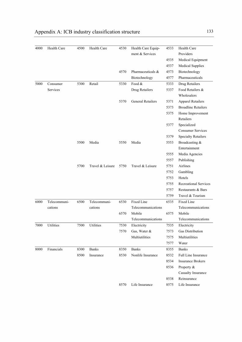
Appendix A: ICB industry classification structure 133

4000 Health Care 4500 Health Care 4530 Health Care Equip-

ment & Services 4533 Health Care

Providers 4535 Medical Equipment 4537 Medical Supplies 4570 Pharmaceuticals & 4573 Biotechnology Biotechnology 4577 Pharmaceuticals

5000 Consumer 5300 Retail 5330 Food & 5333 Drug Retailers Services Drug Retailers 5337 Food Retailers &

Wholesalers 5370 General Retailers 5371 Apparel Retailers 5373 Broadline Retailers 5375 Home Improvement

Retailers 5377 Specialized

Consumer Services 5379 Specialty Retailers 5500 Media 5550 Media 5553 Broadcasting &

Entertainment 5555 Media Agencies 5557 Publishing 5700 Travel & Leisure 5750 Travel & Leisure 5751 Airlines 5752 Gambling 5753 Hotels 5755 Recreational Services 5757 Restaurants & Bars 5759 Travel & Tourism

6000 Telecommuni- cations

6500 Telecommuni- cations

6530 Fixed Line Telecommunications

6535 Fixed Line Telecommunications

6570 Mobile Telecommunications

6575 Mobile Telecommunications

7000 Utilities 7500 Utilities 7530 Electricity 7535 Electricity 7570 Gas, Water & 7573 Gas Distribution Multiutilities 7575 Multiutilities 7577 Water

8000 Financials 8300 Banks 8350 Banks 8355 Banks 8500 Insurance 8530 Nonlife Insurance 8532 Full Line Insurance 8534 Insurance Brokers 8536 Property &

Casualty Insurance 8538 Reinsurance 8570 Life Insurance

8575 Life Insurance

134 Appendix A: ICB industry classification structure 8700 Financial Services 8730 Real Estate 8733 Real Estate &

Development 8737 Real Estate

Investment Trusts 8770 General Financial 8771 Asset Managers 8773 Consumer Finance 8775 Specialty Finance 8777 Investment Services 8779 Mortgage Finance 8980 Equity Investment

Instruments 8985 Equity Investment

Instruments 8990 Nonequity Invest-

ment Instruments 8995 Nonequity Invest-

ment Instruments

9000 Technology 9500 Technology 9530 Software & 9533 Computer Services PC Services 9535 Internet 9537 Software 9570 Hardware & 9572 Computer Hardware Equipment 9574 Electronic Office

Equipment 9576 Semiconductors 9578 Telecommunications

Equipment

Appendix B: U.S. evidence

Sample characteristics and descriptive statistics

Panel A: Sample characteristics

Underlying index Standard & Poor's 500Regional coverage United States Industry classification used Industry Classification BenchmarkStocks within the sample 497Period covered 10 years (1996-2005)

Panel B: Descriptive statistics of the sample

Median Mean 1stquartile

3rdquartile

Number ofobservations

Sales (mio $) 4669 10467 1872 10859 4861EBITDA (mio $) 808 2067 368 1915 4314EBIT (mio $) 606 1642 270 1409 4438Net income (mio $) 323 817 152 731 4382

Total assets (mio $) 6393 28416 2478 18563 4854Invested capital (mio $) 5078 16152 2089 11617 3683Book value of equity (mio $) 2163 4862 1064 5159 4779

Operating cash flow (mio $) 569 1479 257 1320 4574Cash dividend paid (mio $) 126 337 50 326 3605

Panel A presents the characteristics of the U.S. sample. From the 500 stocks within the S&P 500, three stocks (i.e., Dana Corporation, Scientific Atlanta, Sovereign Bank) are excluded because of ambiguous data. Panel B presents the analysis results of the pooled sample of annual data from 1996 to 2005. Annual accounting numbers are as of the beginning of January each year. Negative numbers are excluded.

136 Appendix B: U.S. evidence

Equity value multiples summary statistics

Median Mean 1stquartile

3rdquartile

Number ofobservations

Accrual flow multiplesP / SA 1.6 3.2 0.9 3.1 4729P / GI 4.5 8.1 2.9 7.7 3971P / EBITDA 8.6 15.9 5.4 13.3 4220P / EBIT 11.5 24.8 7.6 17.9 4330P / EBT 14.0 28.9 9.7 22.0 4334P / E 20.8 53.6 14.7 32.8 4277Book value multiplesP / TA 1.1 2.2 0.5 2.3 4729P / IC 1.5 2.2 0.8 2.6 3611P / B 3.1 5.7 2.0 5.2 4664Cash flow multiplesP / OCF 12.3 33.4 7.6 20.6 4465P / D 58.6 341.4 35.0 118.2 3555Knowledge-related multiplesP / (EBIT+R&D) 11.1 16.2 7.8 16.3 969P / (EBIT+AIA) 11.9 18.1 8.2 18.2 1385P / (EBIT+KC) 10.1 12.6 7.2 14.1 729P / (E+R&D) 15.5 22.6 11.3 23.3 951P / (E+AIA) 20.1 29.6 14.4 28.5 1339P / (E+KC) 13.7 17.0 9.7 18.6 706Forward-looking multiplesP / SA 1 1.6 2.4 0.9 3.0 1467P / SA 2 1.5 2.2 0.8 2.8 1461P / EBITDA 1 8.2 11.6 5.3 11.9 1248P / EBITDA 2 7.5 9.4 4.8 10.5 1237P / EBIT 1 11.4 38.9 7.7 16.5 1067P / EBIT 2 10.0 28.1 7.2 13.7 1060P / EBT 1 12.4 20.3 9.1 17.1 1387P / EBT 2 10.8 15.9 8.2 14.3 1414P / E 1 14.7 30.7 11.6 18.4 1226P / E 2 13.7 19.0 10.8 16.6 1171

Equ

ity v

alue

mul

tiple

s

Note: multiples are calculated for each firm i in year t using accounting numbers and mean consen-sus analyst forecasts as of the beginning of January and market prices as of the beginning of April. Criteria for the calculation of multiples and thus inclusion into the summary statistics are: (1) firm i is part of the sample; (2) the market capitalization of firm i is above 200 million U.S. Dollar and the value of net debt is positive in an individual year t; and (3) the underlying value driver x of an individual multiple λ of firm i in year t is positive.

Appendix B: U.S. evidence 137

Absolute valuation accuracy of equity value multiples

Median Mean 1stquartile

3rdquartile

Fraction< 0.15

Fraction< 0.25

Accrual flow multiplesP / SA 0.3987 0.7139 0.1728 0.7368 0.2556 0.3742P / GI 0.3501 0.5480 0.1426 0.6264 0.2721 0.3915P / EBITDA 0.2932 0.5530 0.1218 0.5893 0.3178 0.4734P / EBIT 0.2759 0.4990 0.1086 0.5861 0.3356 0.4831P / EBT 0.2637 0.4073 0.0996 0.5050 0.3513 0.4936P / E 0.2483 0.3904 0.0973 0.4866 0.3584 0.5122Book value multiplesP / TA 0.3949 0.7288 0.1702 0.7209 0.2595 0.3766P / IC 0.3783 0.6930 0.1541 0.7179 0.2708 0.3848P / B 0.3136 0.5092 0.1256 0.5929 0.3170 0.4484Cash flow multiplesP / OCF 0.3226 0.5461 0.1329 0.6146 0.2987 0.4371P / D 0.3890 0.5958 0.1578 0.6810 0.2905 0.4129Knowledge-related multiplesP / (EBIT+R&D) 0.2761 0.3764 0.1022 0.5011 0.3333 0.4758P / (EBIT+AIA) 0.2637 0.5410 0.1049 0.5354 0.3375 0.4972P / (EBIT+KC) 0.2734 0.3810 0.1072 0.5007 0.3442 0.4781P / (E+R&D) 0.2625 0.3691 0.1056 0.4961 0.3295 0.4839P / (E+AIA) 0.2374 0.4903 0.0954 0.4765 0.3795 0.5246P / (E+KC) 0.2642 0.3696 0.1136 0.4897 0.3218 0.4816Forward-looking multiplesP / SA 1 0.3610 0.7664 0.1537 0.7319 0.2743 0.4201P / SA 2 0.3620 0.7579 0.1619 0.6898 0.2649 0.4214P / EBITDA 1 0.2539 0.4261 0.1122 0.4551 0.3658 0.5257P / EBITDA 2 0.2392 0.3951 0.0957 0.4283 0.4011 0.5455P / EBIT 1 0.2468 2.9614 0.1025 0.4559 0.3884 0.5485P / EBIT 2 0.2206 1.2755 0.0933 0.3899 0.4182 0.5845P / EBT 1 0.2269 1.5074 0.1009 0.3977 0.3783 0.5577P / EBT 2 0.1881 0.2645 0.0867 0.3336 0.4394 0.6289P / E 1 0.1710 0.2232 0.0676 0.2981 0.5016 0.6777P / E 2 0.1412 0.2010 0.0535 0.2530 0.5619 0.7376

Equ

ity v

alue

mul

tiple

s

Analysis of absolute valuation errors Fractions

Note: statistical measures of absolute valuation accuracy (median, mean, 1st and 3rd quartile) are based on scaled absolute valuation errors (see equation (5.7)). The fraction <0.15 (<0.25) measures the proportion of scaled absolute valuation errors below 15 percent (25 percent).

138 Appendix B: U.S. evidence

Performance of equity value versus entity value multiples (table)

Absolutedifference

Relativedifference (%)

Absolutedifference

Relativedifference (%)

Overall comparisonEquity value MP vs. Entity value MP -0.0451 -16.12% -0.0086 -4.43%

Accrual flow multiplesP / SA vs. EV / SA -0.0516 -12.95% 0.0229 8.97%P / GI vs. EV / GI -0.0166 -4.74% -0.0084 -3.08%P / EBITDA vs. EV / EBITDA 0.0237 8.07% -0.0298 -9.38%P / EBIT vs. EV / EBIT -0.0107 -3.87% -0.0016 -0.47%

Book value multiplesP / TA vs. EV / TA 0.0189 4.79% -0.0274 -10.58%P / IC vs. EV / IC 0.0451 11.92% -0.0296 -10.91%

Cash flow multiplesP / CFO vs. EV / CFO -0.0528 -16.36% 0.0018 -29.87%

Knowledge-related multiplesP / (EBIT+R&D) vs. EV / (EBIT+R&D) 0.0337 12.20% -0.0544 -16.31%P / (EBIT+AIA) vs. EV / (EBIT+AIA) -0.0068 -2.59% -0.0011 -0.33%P / (EBIT+KC) vs. EV / (EBIT+KC) 0.0450 16.45% -0.0300 -8.73%

Forward-looking multiplesP / SA 1 vs. EV / SA 1 -0.1531 -42.41% 0.0294 10.72%P / SA 2 vs. EV / SA 2 -0.1497 -41.34% 0.0120 4.51%P / EBITDA 1 vs. EV / EBITDA 1 -0.1196 -47.10% -0.0074 -2.01%P / EBITDA 2 vs. EV / EBITDA 2 -0.0768 -32.08% -0.0209 -5.20%P / EBIT 1 vs. EV / EBIT 1 -0.1096 -44.38% 0.0095 2.46%P / EBIT 2 vs. EV / EBIT 2 -0.1402 -63.58% -0.0025 -0.60%

Fraction < 0.15Median valuation errors

Note: negative numbers for the absolute (relative) difference of median valuation errors indicate that equity value multiples outperform entity value multiples. For instance, using the P/SA multiple instead of the EV/SA multiple reduces the absolute (relative) median valuation error on average by 5.16 percentage points (12.95 percent). Positive numbers for the absolute (relative) difference of the fraction <0.15 also indicate that equity value multiples outperform entity value multiples. For instance, using the P/SA multiple instead of the EV/SA multiple increases the fraction of valuation errors below 15 percent on average by 2.29 percentage points in absolute terms and by 8.97 percent in relative terms. For the overall comparison, the average of the individual differences is taken.

Appendix B: U.S. evidence 139

Performance of equity value versus entity value multiples (figure)

68.75%

25.00%

31.25%

75.00%

Median valuation error Fraction <0.15

Entity value MP outperform equity value MPEquity value MP outperform entity value MP

Note: the numbers are based on the relative performance of individual equity value versus entity value multiples in the preceding table (n = 2x16).

140 Appendix B: U.S. evidence

Performance of knowledge-related versus traditional multiples

Medianerror

Fraction< 0.15

Medianerror

Fraction< 0.15

Medianerror

Fraction< 0.15

Traditional accrual flow multiplesP / SA 0.4675 0.2059 6 6 12 12P / GI 0.3791 0.2255 5 5 11 11P / EBITDA 0.3730 0.2422 4 4 10 10P / EBIT 0.3626 0.2670 3 3 9 9P / EBT 0.3545 0.2776 2 1 8 7P / E 0.3451 0.2718 1 2 7 8

Knowledge-related multiplesP / (EBIT+R&D) 0.3143 0.3007 5 5 5 5P / (EBIT+AIA) 0.2820 0.3154 4 4 4 4P / (EBIT+KC) 0.3212 0.2839 6 6 6 6P / (E+R&D) 0.2399 0.3456 1 1 1 1P / (E+AIA) 0.2767 0.3319 3 2 3 2P / (E+KC) 0.2698 0.3287 2 3 2 3

Composite ranking of both multiple typesAbsolute performance

Rankings within thesame multiple type

Note: science based industries are identified on the ICB supersector level (2-digit codes) and in-clude oil & gas (0500), chemicals (1300), basic resources (1700), industrial goods & services (2700), automobiles & parts (3300), personal & household goods (3700), health care (4500), and technology (9500). The calculation of absolute performance numbers is limited to these eight in-dustries.

Appendix B: U.S. evidence 141

Performance of forward-looking versus trailing multiples (table)

Absolutedifference

Relativedifference (%)

Absolutedifference

Relativedifference (%)

Overall comparison1-year forecasts vs. Trailing numbers -0.0440 -15.70% 0.0579 17.16%2-year forecasts vs. Trailing numbers -0.0657 -23.89% 0.0934 27.26%2-year forecasts vs. 1-year forecasts -0.0217 -10.13% 0.0354 8.42%

SalesP / SA 1 vs. P / SA -0.0376 -9.44% 0.0187 7.30%P / SA 2 vs. P / SA -0.0366 -9.18% 0.0093 3.63%P / SA 2 vs. P / SA 1 0.0010 0.29% -0.0094 -3.42%

EBITDAP / EBITDA 1 vs. P / EBITDA -0.0393 -13.39% 0.0480 15.11%P / EBITDA 2 vs. P / EBITDA -0.0539 -18.40% 0.0833 26.20%P / EBITDA 2 vs. P / EBITDA 1 -0.0147 -5.78% 0.0352 9.63%

EBITP / EBIT 1 vs. P / EBIT -0.0291 -10.54% 0.0528 15.74%P / EBIT 2 vs. P / EBIT -0.0553 -20.06% 0.0826 24.62%P / EBIT 2 vs. P / EBIT 1 -0.0263 -10.64% 0.0298 7.67%

EBTP / EBT 1 vs. P / EBT -0.0368 -13.96% 0.0269 7.66%P / EBT 2 vs. P / EBT -0.0756 -28.67% 0.0881 25.07%P / EBT 2 vs. P / EBT 1 -0.0388 -17.09% 0.0612 16.17%

EarningsP / E 1 vs. P / E -0.0774 -31.15% 0.1432 39.97%P / E 2 vs. P / E -0.1072 -43.15% 0.2035 56.79%P / E 2 vs. P / E 1 -0.0298 -17.42% 0.0603 12.02%

Median valuation error Fraction < 0.15

Note: negative numbers for the absolute (relative) difference of median valuation errors indicate that forward-looking multiples outperform trailing multiples. For instance, using the P/E1 multiple instead of the P/E multiple reduces the absolute (relative) median valuation error on average by 7.74 percentage points (31.15 percent). Positive numbers for the absolute (relative) difference of the fraction <0.15 also indicate that forward-looking multiples outperform trailing multiples. For instance, using the P/E1 multiple instead of the P/E multiple increases the fraction of valuation errors below 15 percent on average by 14.32 percentage points in absolute terms and by 39.97 per-cent in relative terms. For the overall comparison, the average of the individual differences is taken.

142 Appendix B: U.S. evidence

Performance of forward-looking versus trailing multiples (figure)

1st1st

2nd3rd

3rd 3rd

1st2nd

2nd

Trailing numbers 1-year forecasts 2-year forecasts

Ran

king

s

1st 2nd 3rd

Note: the three bars indicate first, second, and third ranks of multiples based on trailing numbers, one-year forecasts, and two-year forecasts for pairwise performance evaluations (n = 279) on the ICB sector level (3-digit codes).

Appendix B: U.S. evidence 143

Performance of multiples depending on the industry fineness (table)

Absolutedifference

Relativedifference (%)

Absolutedifference

Relativedifference (%)

Overall comparisonICB sectors vs. ICB supersectors -0.0169 -5.54% 0.0202 6.52%ICB sectors vs. ICB industries -0.0274 -8.60% 0.0566 17.17%ICB supersectors vs. ICB industries -0.0105 -2.89% 0.0365 11.27%

Accrual flow multiplesICB sectors vs. ICB supersectors -0.0222 -7.28% 0.0216 6.85%ICB sectors vs. ICB industries -0.0381 -12.49% 0.0465 14.76%ICB supersectors vs. ICB industries -0.0159 -4.85% 0.0249 8.49%

Book value multiplesICB sectors vs. ICB supersectors -0.0182 -5.01% 0.0234 8.29%ICB sectors vs. ICB industries -0.0280 -7.72% 0.0493 17.46%ICB supersectors vs. ICB industries -0.0098 -2.58% 0.0259 10.00%

Cash flow multiplesICB sectors vs. ICB supersectors -0.0187 -5.26% 0.0337 11.42%ICB sectors vs. ICB industries -0.0413 -11.61% 0.0514 17.43%ICB supersectors vs. ICB industries -0.0226 -6.04% 0.0177 6.79%

Knowledge-related multiplesICB sectors vs. ICB supersectors -0.0135 -5.15% 0.0111 3.27%ICB sectors vs. ICB industries -0.0317 -12.05% 0.0505 14.82%ICB supersectors vs. ICB industries -0.0181 -6.57% 0.0394 11.94%

Forward-looking multiplesICB sectors vs. ICB supersectors -0.0121 -5.02% 0.0111 2.78%ICB sectors vs. ICB industries 0.0021 0.86% 0.0855 21.41%ICB supersectors vs. ICB industries 0.0142 5.60% 0.0744 19.16%

Median valuation error Fraction < 0.15

Note: negative numbers for the absolute (relative) difference of median valuation errors indicate that a finer industry definition outperforms a broader industry definition. For instance, using the ICB sector (3-digit codes) definition instead of the ICB supersector (2-digit codes) definition for accrual flow multiples reduces the absolute (relative) median valuation error on average by 2.22 percentage points (7.28 percent). Positive numbers for the absolute (relative) difference of the frac-tion <0.15 also indicate that a finer industry definition outperforms a broader industry definition. For instance, using the ICB sector (3-digit codes) definition instead of the ICB supersector (2-digit codes) definition for accrual flow multiples increases the fraction of valuation errors below 15 per-cent on average by 2.16 percentage points in absolute terms and by 6.85 percent in relative terms. For the overall comparison, the average of the individual differences is taken.

144 Appendix B: U.S. evidence

Performance of multiples depending on the industry fineness (figure)

3rd

1st

1st 1st

2nd

2nd

2nd3rd3rd

1-digit codes 2-digit codes 3-digit codes

Ran

king

s

1st 2nd 3rd

Note: the three bars indicate first, second, and third ranks of 1-digit, 2-digit, and 3-digit industry codes based on pairwise performance evaluations of 27 equity value multiples for both key per-formance indicators (n = 2x27).

Appendix B: U.S. evidence 145

S&P 500 industry weights

Code Name Weight Code Name Weight

0001 Oil & Gas 9.66% 0500 Oil & Gas 9.66%1000 Basic Materials 2.73% 1300 Chemicals 1.64%

1700 Basic Resources 1.09%2000 Industrials 12.15% 2300 Construction & Materials 0.47%

2700 Industrial Goods & Services 11.68%3000 Consumer Goods 9.27% 3300 Automobiles & Parts 0.54%

3500 Food & Beverage 3.23%3700 Personal & Household Goods 5.50%

4000 Health Care 12.85% 4500 Health Care 12.85%5000 Consumer Services 11.35% 5300 Retail 6.84%

5500 Media 2.65%5700 Travel & Leisure 1.87%

6000 Telecommunications 3.33% 6500 Telecommunications 3.33%7000 Utilities 3.25% 7500 Utilities 3.25%8000 Financials 21.11% 8300 Banks 10.36%

8500 Insurance 4.52%8700 Financial Services 6.23%

9000 Technology 14.29% 9500 Technology 14.29%

ICB industry1-digit codes

ICB supersector2-digit codes

Note: weights are calculated based on market data of the S&P 500 as of February 15, 2006.

146 Appendix B: U.S. evidence

Industry-preferred multiples in U.S. key industries

1st 2nd 3rd 4th 1st 4th

Oil & Gas Median pricing error P / B P / (E+R&D) P / (EBIT+R&D) P / IC 0.2466 0.3747Including forecasts P / E 2 P / E 1 P / B P / EBIT 2 0.1403 0.3100

Fraction < 0.15 P / B P / IC P / (E+R&D) P / (EBIT+R&D) 0.3163 0.2353Including forecasts P / E 2 P / E 1 P / B P / IC 0.5116 0.2500

Industrial Goods & Services Median pricing error P / (E+KC) P / (E+R&D) P / (E+AIA) P / (EBIT+R&D) 0.2539 0.2978Including forecasts P / E 1 P / E 2 P / EBT 2 P / EBIT 2 0.1505 0.2199

Fraction < 0.15 P / (E+R&D) P / (E+KC) P / (EBIT+KC) P / (E+AIA) 0.3254 0.2932Including forecasts P / E 1 P / E 2 P / EBT 2 P / EBT 1 0.4938 0.3617

Health Care Median pricing error P / (E+AIA) P / E P / EBT P / (EBIT+KC) 0.2748 0.2939Including forecasts P / E 2 P / E 1 P / EBT 2 P / EBT 1 0.1989 0.2254

Fraction < 0.15 P / EBIT P / (E+AIA) P / (EBIT+KC) P / EBT 0.3095 0.2951Including forecasts P / E 1 P / E 2 P / EBT 2 P / EBT 1 0.3830 0.3224

Banks Median pricing error P / EBT P / E P / EBIT P / B 0.1530 0.1805Including forecasts P / E 1 P / EBT 2 P / EBT 1 P / E 2 0.0748 0.1062

Fraction < 0.15 P / EBT P / E P / EBIT P / B 0.4926 0.4185Including forecasts P / E 1 P / EBT 2 P / EBT 1 P / E 2 0.7353 0.6531

Technology Median pricing error P / (E+KC) P / (EBIT+KC) P / (E+AIA) P / (EBIT+AIA) 0.2889 0.3428Including forecasts P / E 2 P / E 1 P / EBIT 2 P / (EBIT+KC) 0.2083 0.2889

Fraction < 0.15 P / (E+KC) P / (EBIT+KC) P / IC P / (E+AIA) 0.3000 0.2529Including forecasts P / E 1 P / E 2 P / (E+KC) P / (EBIT+KC) 0.3423 0.2849

Best performing multiples Ranges

Note: performance rankings are constructed for both key performance indicators within five U.S. key industries. The first ranking is always limited to trailing equity value multiples; the second ranking also considers forward-looking equity value multiples. The first four columns list the four best performing multiples in each ranking category. The last two columns report the absolute per-formance of the best and fourth-best performing multiple in each ranking category.

Appendix B: U.S. evidence 147

Correlations among selected value drivers

EBT E BV OCF EBT 2 E 2 EBIT+R&D E+R&D E+AIA E+KC

EBT 1.0000E 0.9910 1.0000BV 0.7580 0.7700 1.0000OCF 0.7830 0.7850 0.7930 1.0000EBT 2 0.9270 0.9260 0.9050 0.8370 1.0000E 2 0.8720 0.8780 0.8850 0.8730 0.9670 1.0000EBIT+R&D 0.8970 0.9000 0.8010 0.9380 0.8880 0.9040 1.0000E+R&D 0.9220 0.9390 0.8500 0.9060 0.9320 0.9360 0.9750 1.0000E+AIA 0.9660 0.9820 0.8250 0.8010 0.9360 0.8950 0.9220 0.9540 1.0000E+KC 0.8970 0.9180 0.8710 0.8980 0.9250 0.9320 0.9730 0.9930 0.9550 1.0000

Note: the correlation matrix shows Pearson correlation coefficients, which are calculated using the pairwise deletion method (n = 668).

148 Appendix B: U.S. evidence

Factors and weights of the two-factor multiples valuation model in U.S. key industries

Multiple 1 Multiple 2 Multiple 1 Multiple 2 Multiple 1 Multiple 2

Oil & GasExcluding forecasts P / (E+R&D) P / B 0.5081 0.4919 0.5000 0.5000

Including forecasts P / E 2 P / B 1.0000 0.0000 1.0000 0.0000

Industrial Goods & ServicesExcluding forecasts P / (E + KC) P / B 0.8473 0.1527 1.0000 0.0000

Including forecasts P / E 2 P / B 0.9592 0.0408 1.0000 0.0000

Health Care Excluding forecasts P / (E+AIA) P / B 0.9211 0.0789 0.9000 0.1000

Including forecasts P / E 2 P / B 0.8712 0.1288 0.9000 0.1000

Banks Excluding forecasts P / EBT P / B 0.5839 0.4161 0.5000 0.5000

Including forecasts P / E 2 P / B 0.9505 0.0495 0.9000 0.1000

Technology Excluding forecasts P / (E+KC) P / B 1.0000 0.0000 1.0000 0.0000

Including forecasts P / E 2 P / B 0.9696 0.0304 1.0000 0.0000

Proposed weightsOptimal weightsFactors

Note: the first factor represents the identified industry-preferred multiple in each industry and cate-gory. Optimal weights are derived by minimizing median absolute valuation errors. The optimiza-tion starts at the fifty-fifty weighting and is subject to the constraints that the weights are positive and add up to one. The proposed weights are derived by personal judgment.

Appendix B: U.S. evidence 149

Performance of single versus combined multiples in selected U.S. key indus-tries

Absolutedifference

Relativedifference (%)

Absolutedifference

Relativedifference (%)

Oil & Gas 2 factor model / proposed vs. Proposed single MP -0.0176 -7.13% 0.0000 -0.02%2 factor model / optimal vs. Proposed single MP -0.0188 -7.61% 0.0000 -0.02%2 factor model / optimal vs. 2 factor model / proposed -0.0012 -0.52% 0.0000 0.00%

Health Care2 factor model / proposed vs. Proposed single MP -0.0212 -7.71% -0.0019 -0.96%2 factor model / optimal vs. Proposed single MP -0.0228 -8.30% -0.0042 -2.11%2 factor model / optimal vs. 2 factor model / proposed -0.0016 -0.64% -0.0023 -1.17%

Banks 2 factor model / proposed vs. Proposed single MP -0.0124 -8.11% -0.0180 -16.92%2 factor model / optimal vs. Proposed single MP -0.0255 -16.66% -0.0290 -27.31%2 factor model / optimal vs. 2 factor model / proposed -0.0131 -9.31% -0.0110 -12.50%

Including forecastsExcluding forecasts

Median absolute valuation errors

Note: negative numbers for the absolute (relative) difference of median valuation errors indicate that combined multiples outperform single multiples. For instance, using combined multiples in the two-factor model with proposed weights instead of proposed single multiples reduces the absolute (relative) median valuation error in the oil & gas industry on average by 1.76 percentage points (7.13 percent) when forecasts are excluded and by 0.003 percentage points (0.02 percent) when forecasts are included.

150 Appendix B: U.S. evidence

Time stability of calibrated absolute valuation errors in the U.S.

0.00

0.25

0.50

0.75

1.00

1.25

1.50

1.75

2.00

2.25

2.50

1996 1997 1998 1999 2000 2001 2002 2003 2004 2005

Cal

ibra

ted

valu

atio

n er

ror

1st quartile Median absolute valuation error 3rd quartile

Note: to illustrate the time stability of valuation accuracy, calibrated performance indicators (me-dian absolute valuation error, 1st and 3rd quartile) are calculated in each year from 1996 to 2005 for eleven representative equity value multiples. The arithmetic mean is used for the aggregation of performance indicators.

Appendix C: Definition of variables

Appendix C describes how the variables used to construct the multiples in the empirical study are defined. All financial statement, price, and forecast data is ob-tained from Thomson Financial in Zurich. Historical financial data is based on the Worldscope (WC) database, price data on the Datastream (DS) database, and ana-lyst forecasts on the Institutional Brokers Estimate Service (I/B/E/S) database. Variable definitions except for those labeled are taken out of the database descrip-tions (Datastream (1996), I/B/E/S (2000), and Thomson Financial (2003)). The #s in parentheses refer to data items of DS, I/B/E/S, and WC.

Market price variables

• * Market value of common equity or market capitalization (P) represents the market value of a firm’s outstanding common equity. P is calculated by multi-plying the current number of common shares outstanding by the latest closing stock price (DS #MV). In the text, P sometimes also refers to the stock price itself.

• * Enterprise value (EV) represents the market value of a firm as a whole. EV is calculated as the sum of the market value of common equity (DS #MV) and the book value of net debt (ND), where ND equals book value of total debt (WC #03255) minus cash & equivalents (WC #02001) plus preferred stock (WC #03451).

Variables used to construct accrual flow multiples

• (Net) sales or revenues (SA) represent gross sales and other operating revenue less discounts, returns and allowances (WC #01001).

• Gross income (GI) represents the difference between sales or revenues and cost of goods sold (WC #01100).

• Earnings before interest, taxes, depreciation, and amortization (EBITDA) rep-resent the earnings of a firm before interest expense, income taxes, deprecia-tion, and amortization. It is calculated by taking the pre-tax income and adding

152 Appendix C: Definition of variables

back interest expense on debt and depreciation, depletion, and amortization, and subtracting interest capitalized (WC #18198).

• Earnings before interest and taxes (EBIT) represent the earnings of a firm be-fore interest expense and income taxes. It is calculated by taking the pre-tax income, adding back interest expense on debt, and subtracting interest capital-ized (WC #18191).

• Earnings before taxes (EBT) or pre-tax income represent all income or loss be-fore any federal, state or local taxes (WC #01401).

• Earnings (E) or net income available to common shareholders (NI) represent net income after all operating and non-operating income and expense, re-serves, income taxes, minority interest, and extraordinary items (WC #01751).

Variables used to construct book value multiples

• Total assets (TA) represent the sum of total current assets, long term receiv-ables, investment in unconsolidated subsidiaries, other investments, net prop-erty plant and equipment, and other assets (WC #02999).

• Book value of common equity (B) represents common shareholders' invest-ment in a firm (WC #03501). It is the difference between total assets (WC #02999) and the book value of total debt (WC #03255).

• Invested capital (IC) equals total assets (WC #02999) minus cash & equiva-lents (WC #02001). IC represents the cumulative amount a firm has invested in its core operations.

Variables used to construct cash flow multiples

• Operating cash flow or cash flow from operating activities (OCF) represents the net cash receipts and disbursements resulting from the operations of a firm (WC #04860).

• Ordinary cash dividends (D) represent the total cash dividends paid on a firm’s common stock during a fiscal year, including extra and special dividends (WC #18192).

Appendix C: Definition of variables 153

Variables used to construct knowledge-related multiples

• Research and development expenditures (R&D) represent all direct and indi-rect costs related to the creation and development of new processes, tech-niques, applications, and products with commercial possibilities (WC #01201).

• Amortization of intangible assets (AIA) represents the cost allocation for in-tangible assets such as patents, leasehold improvements, trademarks, book-plates, tools, and film costs (WC #01149).

• * Knowledge costs (KC) equal R&D expenditures (WC #01201) plus amorti-zation of intangible assets (WC #01149). KC serve as a proxy of a firm’s cost for the creation and maintenance of intangible assets.

Variables used to construct forward-looking multiples

Forward-looking multiples are constructed for five value drivers from the in-come statement: SA, EBITDA, EBIT, EBT, and E. The fiscal year to which a fore-cast applies is identified in the forecast period indicator (FPI) variable: if FPI = 1, the forecast is for the current fiscal year (fiscal year 1) and if FPI = 2, it is for the next fiscal year (fiscal year 2). All forecasts represent mean consensus estimates of financial analysts recorded by I/B/E/S.

• SA 1 and SA 2 (I/B/E/S #SAL1 and #SAL2)

• EBITDA 1 and EBITDA 2 (I/B/E/S #EBD1 and #EBD2)

• EBIT 1 and EBIT 2 (I/B/E/S #EBT1 and #EBT2)

• EBT 1 and EBT 2 (I/B/E/S #PPS1 and #PPS2)

• E 1 and E 2 (I/B/E/S #INC1 and #INC2)

References

Aboody, D., 2006. Financial Statement Analysis: Free Cash Flows. Lecture notes, UCLA.

Aboody, D., Lev, B., 1998. The Value Relevance of Intangibles: The Case of Soft-ware Capitalization. Journal of Accounting Research 36, 161-191.

Aboody, D., Lev, B., 2000. Information Asymmetry, R&D, and Insider Gains. Journal of Finance 55, 2747-2766.

Achleitner, A.-K, 2002. Handbuch Investment Banking, 3rd edition. Gabler, Wies-baden, Germany.

Alford, A.W., 1992. The Effect of the Set of Comparable Firms on the Accuracy of the Price-Earnings Valuation Method. Journal of Accounting Research 30, 94-108.

Ali, A., Hwang, L.-S., 2000. Country-Specific Factors Related to Financial Report-ing and the Value Relevance of Accounting Data. Journal of Accounting Re-search 38, 1-21.

Amir, E., Lev, B., 1996. Value-relevance of nonfinancial information: The wireless communication industry. Journal of Accounting and Economics 22, 3-30.

Arzac, E.R., 2005. Valuation for Mergers, Buyouts, and Restructuring. Wiley, Ho-boken, NJ.

Baker, M., Ruback, R.S., 1999. Estimating Industry Multiples. Working paper, Harvard University.

Ball, R., Brown, P., 1968. An Empirical Evaluation of Accounting Income Num-bers. Journal of Accounting Research 6, 159-178.

Ballwieser, W., 2004. Unternehmensbewertung: Prozess, Methoden und Probleme. Schäffer Poeschel, Stuttgart, Germany.

References 155

Barclay, M.J., Smith, C.W., 2005. The Capital Structure Puzzle: The Evidence Re-

visited. Journal of Applied Corporate Finance 17, 8-17.

Barker, R.G., 1999a. Survey and Market-based Evidence of Industry-dependence in Analysts’ Preferences Between the Dividend Yield and Price-earnings Ratio Valuation Models. Journal of Business and Accounting 26, 393-418.

Barker, R.G., 1999b. The role of dividends in valuation models used by analysts and fund managers. European Accounting Review 8, 195-218.

Barth, M.E., Beaver, W.H., Hand, J.R.M., Landsman, W.R., 2004. Accruals, Ac-counting-Based Valuation Models, and the Prediction of Equity Values. Working paper, Stanford University, University of North Carolina at Chapel Hill.

Basu, S., 1997. The conservatism principle and the asymmetric timeliness of earn-ings. Journal of Accounting and Economics 24, 3-37.

Beatty, R.P., Riffe, S.M., Thompson, R., 1999. The Method of Comparables and Tax Court Valuations of Private Firms: An Empirical Investigation. Account-ing Horizons 13, 177-199.

Beaver, W.H., Morse, D., 1978. What determines price-earnings ratios? Financial analysts Journal 34, 65-78.

Begley, J., Feltham, G.A., 2002. The Relation between Market Values, Earnings Forecasts, and Reported Earnings. Contemporary Accounting Research 19, 1-48.

Benninga, S.Z., Sarig, O.H., 1997. Corporate Finance: A Valuation Approach. McGraw-Hill, New York, NY.

Berkman, H., Bradhury, M.E., Ferguson, J., 2000. The Accuracy of Price-Earnings and Discounted Cash Flow Methods of IPO Equity Valuation. Journal of In-ternational Financial Management and Accounting 11, 71-83.

156 References Bernard, V.L., Thomas, J.K., 1989. Post-Earnings-Announcement Drift: Delayed

Price Response or Risk Premium? Journal of Accounting Research 27, 1-36.

Bernard, V.L., Thomas, J.K., 1990. Evidence that stock prices do not fully reflect the implications of current earnings for future earnings. Journal of Accounting and Economics 13, 305-340.

Berndt, T., 2005. Financial Reporting: Grundlagen des Financial Reporting. Lecture notes, University of St.Gallen.

Bhojraj, S., Lee, C.M.C., 2002. Who Is My Peer? A Valuation Based Approach to the Selection of Comparable Firms. Journal of Accounting Research 40, 407-439.

Bhojraj, S., Lee, C.M.C., Ng, D.T., 2003. International Valuation Using Smart Mul-tiples. Working paper, Cornell University.

Bhojraj, S., Lee, C.M.C., Oler, D.K., 2003. What’s My Line? A Comparison of In-dustry Classification Schemes for Capital Market Research. Journal of Ac-counting Research 41, 745-774.

Block, S.B., 1999. A Study of Financial Analysts: Practice and Theory. Financial Analysts Journal 55, 86-95.

Boatsman, J., Baskin, E., 1981. Asset Valuation with Incomplete Markets. Account-ing Review 56, 38-53.

Bonadurer, W., 2003. Valuation by Multiples. Doctoral seminar paper, University of St.Gallen.

Bradshaw, M.T., 2002. The Use of Target Prices to Justify Sell-Side Analysts’ Stock Recommendations. Accounting Horizons 16, 27-41.

Bradshaw, M.T., 2004. How Do Analysts Use Their Earnings Forecasts in Generat-ing Stock Recommendations? Accounting Review 79, 25-50.

References 157

Brealy, R.A., Myers, S.C., 2000. Principles of Corporate Finance, 6th edition.

McGraw-Hill, New York, NY.

Burgstahler, D.C., 1998. Discussion of “Combining Earnings and Book Value in Equity Valuation.” Contemporary Accounting Research 15, 325-341.

Carter, R.B., Van Auken, H.E., 1990. Security analysis and portfolio management: A survey and analysis. Journal of Portfolio Management 16, 81-85.

Chan, L.K., Lakonishok, J., Sougiannis, T., 2001. The Stock Market Valuation of Research and Development Expenditures. Journal of Finance 56, 2431-2456.

Chang, J., 1999. The decline in value relevance of earnings and book values. Work-ing paper, University of Pennsylvania.

Cheng, C.S.A., McNamara, R., 2000. The Valuation Accuracy of the Price-Earnings and Price-Book Benchmark Valuation Methods. Review of Quantita-tive Finance and Accounting 15, 349-370.

Cochrane, J.H., 2005. Writing Tips for Ph.D. Students. Working paper, University of Chicago.

Coenenberg, A.G., Schultze, W., 2002. Das Multiplikator-Verfahren in der Unternehmensbewertung: Konzeptionen und Kritik. Finanz Betrieb 12, 697-703.

Collins, D.W., Maydew, E.L., Weiss, I.S., 1997. Changes in the value-relevance of earnings and book values over the past forty years. Journal of Accounting and Economics 24, 39-67.

Copeland, T., Koller, T., Murrin, J., 2000. Valuation: Measuring and Managing the Value of Companies, 3rd edition. Wiley, Hoboken, NJ.

Copeland, T., Weston, J.F., Shastri, K., 2004. Financial Theory and Corporate Pol-icy, 4th edition. Addison-Wesley, Boston, MA.

158 References Damodaran, A., 2001. The Dark Side of Valuation: Valuing Old Tech, New Tech,

and New Economy Companies. FT Prentice Hall, Upper Saddle River, NJ. Manuscript provided by the author, http://www.damodaran.com, April 04, 2006.

Damodaran, A., 2002. Investment Valuation: Tools and Techniques for Determin-ing the Value of Any Asset. Wiley, Hoboken, NJ. Manuscript provided by the author, http://www.damodaran.com, April 04, 2006.

Damodaran, A., 2006. Damodaran on Valuation, 2nd edition. Wiley, Hoboken, NJ. Manuscript provided by the author, http://www.damodaran.com, April 04, 2006.

Datastream, 1996. Datatype definitions. http://www.thomson.com/financial, Febru-ary 22, 2006.

DeAngelo, L.E., 1990. Equity Valuation and Corporate Control. Accounting Re-view 65, 93-112.

Dechow, P.M., Hutton, A.P., Sloan, R.G., 1999. An empirical assessment of the residual income valuation model. Journal of Accounting and Economics 26, 1-34.

Demirakos, E.G., Strong, N.C., Walker, M., 2004. What Valuation Models Do Ana-lysts Use? Accounting Horizons 18, 221-240.

Dow Jones, 2006. Dow Jones STOXX 600: Factsheet. http://www.stoxx.com, Sep-tember 02, 2006.

Easton, P.D., Harris, T., 1991. Earnings as an Explanatory Variable for Returns. Journal of Accounting Research 29, 19-36.

Easton, P.D., 2004a. Discussion of Forward Versus Trailing Earnings in Equity Valuation. Review of Accounting Studies 9, 330-336.

References 159

Easton, P.D., 2004b. PE Ratios, PEG Ratios, and Estimating the Implied Expected

Rate of Return on Equity Capital. Accounting Review 79, 73-95.

Eberhart, A.C., 2001. Comparable firms and the precision of equity valuations. Journal of Banking and Finance 25, 1367-1400.

Eberhart, A.C., 2004. Equity Valuation Using Multiples. Journal of Investing 13, 48-54.

Eberhart, A.C., Maxwell, W.F., Siddique, A.R., 2004. An Examination of Long-Term Abnormal Stock Returns and Operating Performance Following R&D Increases. Journal of Finance 59, 623-650.

Eccles, G.E., Herz, R.H., Keegan, E.M., Phillips, D.M.H., 2002. The Value Report-ing Revolution: Moving Beyond the Earnings Game, German edition. Wiley, Weinheim, Germany.

Edwards, E.O., Bell, P.W., 1961. The Theory and Measurement of Business In-come. University of California Press, Berkeley, CA.

Esty, B.C., 2000. What Determines Comparability When Valuing Firms With Mul-tiples? Journal of Financial Education 2, 24-33.

Evans, F.C., Bishop, D.M., 2001. Valuation for M&A: Building Value in Private Companies. Wiley, Hoboken, NJ.

Fahrmeir, L., Künstler, R., Pigeot, I., Tutz, G., 1999. Statistik: Der Weg zur Datenanalyse, 2nd edition. Springer, Berlin, Germany.

Fairfield, P.M., 1994. P/E, P/B and the Present Value of Future Dividends. Finan-cial Analysts Journal 50, 23-31.

Fama, E.F., 1970. Efficient Capital Markets: A Review of Theory and Empirical Work. Journal of Finance 25, 383-417.

160 References Fama, E.F., 1976. Foundations of Finance. Basic Books, New York, NY.

Fama, E.F., 1991. Efficient Capital Markets: II. Journal of Finance 46, 1575-1617.

Fama, E.F., 1998. Market efficiency, long-term returns, and behavioral finance. Journal of Financial Economics 49, 283-306.

Fama, E.F., French, K.R., 1992. The Cross-section of Expected Stock Returns. Journal of Finance 47, 427-466.

Fama, E.F., French, K.R., 1993. Common risk factors in the returns on stocks and bonds. Journal of Financial Economics 33, 3-56.

Fama, E.F., French, K.R., 1995. Size and Book-to-Market Factors in Earnings and Returns. Journal of Finance 50, 131-156.

Fama, E.F., French, K.R., 1997. Industry Costs of Equity. Journal of Financial Eco-nomics 43, 153-193.

Fama, E.F., French, K.R., 1998. Value versus Growth: The International Evidence. Journal of Finance 53, 1975-1999.

Feltham, G.A., Ohlson, J.A., 1995. Valuation and Clean Surplus Accounting for Operating and Financial Activities. Contemporary Accounting Research 11, 689-731.

Fernández, P., 2002. Valuation Methods and Shareholder Value Creation. Aca-demic Press, San Diego, CA.

Francis, J., Schipper, K., 1999. Have Financial Statements Lost Their Relevance? Journal of Accounting Research 37, 319-352.

Francis, J., Schipper, K., Vincent, L., 2003. The Relative and Incremental Explana-tory Power of Earnings and Alternative (to Earnings) Performance Measures for Returns. Contemporary Accounting Research 20, 121-164.

References 161

Frankel, R., Lee, C.M.C., 1998. Accounting valuation, market expectation, and

cross-sectional stock returns. Journal of Accounting and Economics 25, 283-319.

Frykman, D., Tolleryd, J., 2003. Corporate Valuation: An Easy Guide to Measuring Value. FT Prentice Hall, Upper Saddle River, NJ.

Geddes, R., 2003. IPOs and Equity Offerings. Butterworth-Heinemann, Burlington, MA.

Gibson, C.H., 1998. Financial Statement Analysis: Using Accounting Information, 8th edition. South-Western, Cincinnati, OH.

Gilson, S.C., Hotchkiss, E.S., Ruback, R.S., 2000. Valuation of bankrupt firms. Re-view of Financial Studies 13, 43-74.

Gjesdal, F., 2004. A Steady State Growth Valuation Model: A Note on Accounting and Valuation. Working paper, Norwegian School of Economics and Busi-ness, Bergen.

Goedhart, M., Koller, T., Wessels, D., 2005. The right role for multiples in valua-tion. McKinsey on Finance 15, 7-11.

Gode, D., Ohlson, J.A., 2006. A Unified Valuation Framework for Dividends, Free-Cash Flows, Residual Income, and Earnings Growth Based Models. Working paper, New York University, Arizona State University.

Gordon, M., 1962. The Investment, Financing, and Valuation of the Corporation. Irwin, Homewood, IL.

Guenther, D.A., Rosman, A.J., 1994. Difference between Compustat and CRSP SIC Codes and Related Effects on Research. Journal of Accounting and Economics 18, 115-128.

162 References Guo, R.-J., Lev, B., Shi, C., 2006. Explaining the Short- and Long-Term IPO

Anomalies by R&D. Journal of Business Finance and Accounting 33, 550-579.

Hand, J.R.M., 1999. Profits, Losses, and the Stock of Internet Firms. Working pa-per, University of North Carolina at Chapel Hill.

Hand, J.R.M., 2000. The Role of Economic Fundamentals, Web Traffic, and Supply and Demand in the Pricing of US Internet Stocks. Working paper, University of North Carolina at Chapel Hill.

Harrington, D.R., 2004. Corporate Financial Analysis in a Global Environment, 7th edition. Thomson South-Western, Mason, OH.

Herrmann, V., 2002. Marktpreisschätzung mit kontrollierten Multiplikatoren. Josef Eul Verlag, Cologne, Germany.

Herrmann, V., Richter, F., 2003. Pricing with Performance-Controlled Multiples. Schmalenbach Business Review 55, 194-219.

I/B/E/S International, 2000. The I/B/E/S Glossary: A Guide to Understanding I/B/E/S Terms and Conventions. http://www.thomson.com/financial, February 22, 2006.

ICB, 2004. Product Specification ICB Universe Data Services. http://www.icbenchmark.com, January 27, 2006.

Ittner, C.D., Larcker, D.F., 1998. Are Nonfinancial Measures Leading Indicators of Financial Performance? An Analysis of Customer Satisfaction. Journal of Ac-counting Research 36, 1-35.

Jensen, M.C., 1986. Agency Costs of Free Cash Flow, Corporate Finance, and Takeovers. American Economic Review 76, 323-329.

Johnson, L.T., Petrone, K.R., 1998. Commentary: Is Goodwill an Asset? Account-ing Horizons 12, 293-303.

References 163

Kahle, K.M., Walkling, R.A., 1996. The Impact of Industry Classifications on Fi-

nancial Research. Journal of Financial and Quantitative Analysis 31, 309-335.

Kaplan, S.N., Ruback, R.S., 1995. The Valuation of Cash Flow Forecasts: An Em-pirical Analysis. Journal of Finance 50, 1059-1093.

Kaplan, S.N., Ruback, R.S., 1996. The Market Pricing of Cash Flow Forecasts: Discounted Cash Flow vs. the Method of Comparables. Journal of Applied Corporate Finance 8, 45-60.

Kim, M., Ritter, J.R., 1999. Valuing IPOs. Journal of Financial Economics 53, 409-437.

Kothari, S.P., 2001. Capital markets research in accounting. Journal of Accounting and Economics 31, 105-231.

Koller, T., Goedhart, M., Wessels, D., 2005. Valuation: Measuring and Managing the Value of Companies, 4th edition. Wiley, Hoboken, NJ.

Krolle, S., Schmitt, G., Schwetzler, B., editors, 2005. Multiplikatorverfahren in der Unternehmensbewertung: Anwendungsberichte, Problemfälle, Lösungsalter-nativen. Schäffer-Poeschel, Stuttgart, Germany.

Lee, C.M.C., 1996. Measuring wealth. CA Magazine 129, 32-37.

Lee, C.M.C., Myers, J., Swaminathan, B., 1999. What Is the Intrinsic Value of the Dow? Journal of Finance 54, 1693-1741.

Lev, B., 1989. On the Usefulness of Earnings and Earnings Research: Lessons and Directions from Two Decades of Empirical Research. Journal of Accounting Research 27, 153-192.

Lev, B., 2001. Intangibles: Management, Measurement, and Reporting. Brookings, Washington, DC.

Lev, B., Sougiannis, T., 1996. The capitalization, amortization, and value-relevance of R&D. Journal of Accounting and Economics 21, 107-138.

164 References Lev, B., Nissim, D., Thomas, J.K., 2002. On the usefulness of R&D capitalization

and amortization. Working paper, New York University, Columbia University, Yale University.

Lie, E., Lie, H.J., 2002. Multiples Used to Estimate Corporate Value. Financial Analysts Journal 58, 44-54.

Liu, J., Thomas, J.K., 2000. Stock Returns and Accounting Earnings. Journal of Accounting Research 38, 71-101.

Liu, J., Nissim, D., Thomas, J.K., 2002a. Equity Valuation Using Multiples. Journal of Accounting Research 40, 135-172.

Liu, J., Nissim, D., Thomas, J.K., 2002b. International equity valuation using multi-ples. Working paper, UCLA, Columbia University, Yale University.

Liu, J., Nissim, D., Thomas, J.K., 2005a. Cash flow is King? Comparing valuations based on cash flow versus earnings multiples. Working paper, UCLA, Colum-bia University, Yale University.

Liu, J., Nissim, D., Thomas, J.K., 2005b. Value relevance of cash flows versus earnings: an international analysis using multiples. Working paper, UCLA, Columbia University, Yale University.

Loderer, C., Jörg, P., Pichler, K., Zgraggen, P., 2005. Handbuch der Bewertung: Praktische Methoden und Modelle zur Bewertung von Projekten, Unternehmen und Strategien, 3rd edition. NZZ Verlag, Zurich.

Löhnert, P.G., Böckmann, U.J., 2005. Multiplikatorverfahren in der Unter-nehmensbewertung. In Peemoeller, V.H., editor. Praxishandbuch der Unter-nehmensbewertung, 3rd edition, 403-428. Verlag Neue Wirtschafts-Briefe, Berlin, Germany.

Lundholm, R., Sloan, R.G., 2004. Equity Valuation and Analysis with eVal. McGraw-Hill, New York, NY.

References 165

Lynch, P., 2000. One Up on Wall Street. Simon and Schuster, New York, NY.

Marshall, A., 1898. Principles of Economics, 4th edition. Macmillan, London, UK.

Miller, M.H., Modigliani, F., 1961. Dividend Policy, Growth and the Valuation of Shares. Journal of Business 34, 411-433.

Mintzberg, H., Lampel, J., Ahlstrand, B., 1998: Strategy Safari: A Guided Tour Through The Wilds of Strategic Management. Free Press, New York, NY.

Modigliani, F., Miller, M.H., 1958. The Cost of Capital, Corporation Finance, and the Theory of Investment. American Economic Review 48, 261-297.

Modigliani, F., Miller, M.H., 1963. Corporate Income Taxes and the Cost of Capi-tal: A Correction. American Economic Review 53, 433-443.

Moxter, A., 1983. Grundsätze ordnungsgemässer Unternehmensbewertung, 2nd edition. Gabler, Wiesbaden, Germany.

Mueller, G.G., Gernon, H., Meek, G, 1994. Accounting: An International Perspec-tive. Irwin, New York, NY.

Müller-Stewens, G., Lechner, C., 2001. Strategisches Management: Wie strategische Initiativen zum Wandel führen, Der St.Galler Management Navigator. Schäffer-Poeschel, Stuttgart, Germany.

Myers, S.C., 1977. Determinants of Corporate Borrowing. Journal of Financial Economics 5, 147-175.

Myers, S.C., 1984. The Capital Structure Puzzle. Journal of Finance 39, 575-592.

Nelson, J.M., 2006. Intangible Assets, Book-to-Market, and Common Stock Re-turns. Journal of Financial Research 29, 21-41.

Nissim, D., Penman, S.H., 2001. Ratio Analysis and Equity Valuation: From Re-search to Practice. Review of Accounting Studies 6, 109-154.

166 References O’Hanlon, J., Peasnell, K.V., 2002. Residual Income and Value-Creation: The

Missing Link. Review of Accounting Studies 7, 229-245.

Ohlson, J.A., 1995. Earnings, Book Values, and Dividends in Equity Valuation. Contemporary Accounting Research 11, 661-687.

Ohlson, J.A., 2002. Discussion of “Residual Income and Value-Creation: The Miss-ing Link.” Review of Accounting Studies 7, 247-251.

Ohlson, J.A., 2005. On Accounting-Based Valuation Formulae. Review of Ac-counting Studies 10, 323-347.

Ohlson, J.A., Juettner-Nauroth, B., 2005. Expected EPS and EPS Growth as Deter-minants of Value. Review of Accounting Studies 10, 349-365.

Palepu, K.G., Healy, P.M., Bernard, V.L., 2000. Business Analysis and Valuation Using Financial Statements, 2nd edition. South-Western, Cincinnati, OH.

Peasnell, K.V., 1981. On capital budgeting and income measurement. Abacus 17, 52-67.

Peasnell, K.V., 1982. Some formal connections between economic values and yields and accounting numbers. Journal of Business, Finance and Accounting 9, 361-381.

Peemöller, V. H., Kunowski, S., Hillers, J., 1999. Ermittlung des Kapitalisierungs-zinssatzes für internationale Mergers and Acquisitions bei Anwendung des Discounted Cash Flow Verfahrens. Die Wirtschaftsprüfung 52, 621-630.

Penman, S.H., 1996. The Articulation of Price-Earnings Ratios and Market-to-Book Ratios and the Evaluation of Growth. Journal of Accounting Research 34, 235-259.

Penman, S.H., 1998. Combining Earnings and Book Value in Equity Valuation. Contemporary Accounting Research 15, 291-324.

References 167

Penman, S.H., 2004. Financial Statement Analysis and Security Valuation, 2nd edi-

tion. McGraw-Hill, New York, NY.

Penman, S.H., 2006. Handling Valuation Models. Journal of Applied Corporate Finance 18, 48-55.

Penman, S.H., Sougiannis, T., 1998. A Comparison of Dividend, Cash Flow, and Earnings Approaches to Equity Valuation. Contemporary Accounting Re-search 15, 343-383.

Pereiro, L.E., 2002. Valuation of Companies in Emerging Markets: A Practical Ap-proach. Wiley, Hoboken, NJ.

Pfeil, O.P., 2003. The Valuation of Intellectual Capital. Working paper, MIT, Uni-versity of St.Gallen.

Pfeil, O.P., 2004. Earnings from Intellectual Capital as a Driver of Shareholder Value. Haupt, Bern, Switzerland.

Pratt, S., 2005. The Market Approach to Valuing Businesses, 2nd edition. Wiley, Hoboken, NJ.

Pratt, S., Reilly, R., Schweihs, R., 2000. Valuing a Business, 3rd edition. Irwin, Homewood, IL.

Preinreich, G.A.D., 1938. Annual survey of economic theory: The theory of depre-ciation. Econometrica 6, 219-241.

Rappaport, A., 1981. Selecting strategies that create shareholder wealth. Harvard Business Review 59, 139-149.

Richter, F., 2005. Mergers and Acquisitions: Investmentanalyse, Finanzierung und Prozessmanagement. Vahlen, Munich, Germany.

Ross, S.A., 1977. Determination of Financial Structure: The Incentive Signaling Approach. Bell Journal of Economics 8, 23-40.

168 References Ross, S.A., Westerfield, R.W., Jaffe, J., 2002. Corporate Finance, 6th edition.

McGraw-Hill, New York, NY.

Smith, C.W., 1986. Investment Banking and the Capital Acquisition Process. Jour-nal of Financial Economics 15, 3-29.

Smith, C.W., Ikenberry, D., Nayar, A., Anda, J., McVey, M., Stewart, G.B., 2005. Morgan Stanley Roundtable on Capital Structure and Payout Policy. Journal of Applied Corporate Finance 17, 36-54.

Spremann, K., 2002. Finanzanalyse und Unternehmensbewertung. Oldenbourg, Munich, Germany.

Spremann, K., 2004. Valuation: Grundlagen moderner Unternehmensbewertung. Oldenbourg, Munich, Germany.

Spremann, K., 2005. Modern Finance, 2nd edition. Oldenbourg, Munich, Germany.

Spremann, K., 2006. Portfoliomanagement, 3rd edition. Oldenbourg Munich, Ger-many. Manuscript provided by the author.

Stahel, W. A., 2002. Statistische Datenanalyse: Eine Einführung für Naturwissen-schaftler, 4th edition. Vieweg, Braunschweig, Germany.

Standard & Poor’s, 2006. S&P 500: Factsheet. http://www.standardandpoors.com, September 02, 2006.

Stewart, G.B., 1991. The Quest for Value. Harper Business, New York, NY.

Suozzo, P., Cooper, S., Sutherland, G., Deng, Z., 2001. Valuation Multiples: A Primer. Research report, UBS Investment Bank.

Tasker, S.C., 1998. Industry-preferred Multiples in Acquisition Valuation. Working paper, Cornell University.

Thomas, J.K., Zhang, H., 2004. Another look at P/E ratios. Working paper, Yale University, University of Hong Kong.

References 169

Thomson Financial, 2003. Worldscope Database: Datatype Definitions Guide.

http://www.thomson.com/financial, February 22, 2006.

Trueman, B., Wong, M.H.F., Zhang, X.-J., 2000. The Eyeballs Have It: Searching for the Value in Internet Stocks. Journal of Accounting Research 38, 137-162.

Trueman, B., Wong, M.H.F., Zhang, X.-J., 2001. Back to Basics: Forecasting the Revenues of Internet Firms. Review of Accounting Studies 6, 305-329.

Von Berenberg-Consbruch, J., 2006. Industriespezifische Multiples in der Unter-nehmensbewertung: eine empirische Untersuchung für den europäischen Aktienmarkt. Master thesis, University of St.Gallen.

White, G.I., Sondhi, A.C., Fried, D., 2003. The Analysis and Use of Financial Statements, 3rd edition. Wiley, Hoboken, NJ.

Williams, J., 1938. The Theory of Investment Value. Harvard University Press, Cambridge, MA.

Yee, K.K., 2004. Forward Versus Trailing Earnings in Equity Valuation. Review of Accounting Studies 9, 301-329.

Curriculum Vitae

Name: Andreas Schreiner Born: January 29, 1982 in Graz, Austria

Education

2004 – 2007 University of St.Gallen, Switzerland Doctoral Studies in Banking and Corporate Finance (Dr. oec.) 2006 – 2007 UCLA Anderson School of Management, Los Angeles, U.S. Yale University, School of Management, New Haven, U.S. 2001 – 2004 University of Graz, Austria Undergraduate / Graduate Studies in Business (B.A., M.A.) 2004 University of St.Gallen, Switzerland

Practical experience

2004 – 2006 Swiss Institute of Banking and Finance, St. Gallen, Switzerland Research Associate of Professor Klaus Spremann

2004 Kuehne-Institute of Logistics, St. Gallen, Switzerland Project Associate, Consulting and Research 2004 Graypen GP Shipping, Southampton, United Kingdom Intern, Shipping Brokerage 2003 GEFO Gesellschaft für Öltransporte, Hamburg, Germany Intern, Global Shipping 2002 Bayer Business Services, Neuss and Leverkusen, Germany Intern, Inhouse Consulting