Machine Learning Crash Course - Georgia Institute of …hays/compvision/lectures/1… · ·...
65
Machine Learning Crash Course Computer Vision James Hays Slides: Isabelle Guyon, Erik Sudderth, Mark Johnson, Derek Hoiem Photo: CMU Machine Learning Department protests G20
Transcript of Machine Learning Crash Course - Georgia Institute of …hays/compvision/lectures/1… · ·...

Machine Learning Crash Course
Computer VisionJames Hays
Slides: Isabelle Guyon,
Erik Sudderth,
Mark Johnson,
Derek Hoiem
Photo: CMU Machine Learning
Department protests G20


Dimensionality Reduction
• PCA, ICA, LLE, Isomap, Autoencoder
• PCA is the most important technique to know. It takes advantage of correlations in data dimensions to produce the best possible lower dimensional representation based on linear projections (minimizes reconstruction error).
• PCA should be used for dimensionality reduction, not for discovering patterns or making predictions. Don't try to assign semantic meaning to the bases.


• http://fakeisthenewreal.org/reform/

• http://fakeisthenewreal.org/reform/

Clustering example: image segmentation
Goal: Break up the image into meaningful or perceptually similar regions

Segmentation for feature support or efficiency
[Felzenszwalb and Huttenlocher 2004]
[Hoiem et al. 2005, Mori 2005][Shi and Malik 2001]
Slide: Derek Hoiem
50x50
Patch
50x50
Patch

Segmentation as a result
Rother et al. 2004
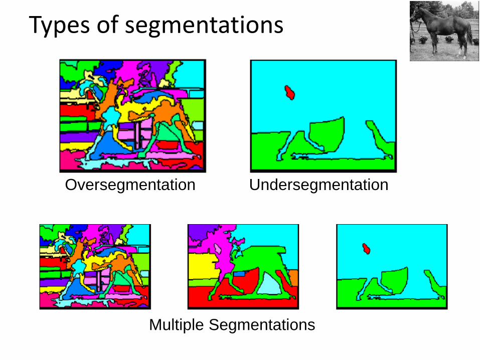
Types of segmentations
Oversegmentation Undersegmentation
Multiple Segmentations

Clustering: group together similar points and represent them with a single token
Key Challenges:
1) What makes two points/images/patches similar?
2) How do we compute an overall grouping from pairwise similarities?
Slide: Derek Hoiem

How do we cluster?
• K-means– Iteratively re-assign points to the nearest cluster
center
• Agglomerative clustering– Start with each point as its own cluster and iteratively
merge the closest clusters
• Mean-shift clustering– Estimate modes of pdf
• Spectral clustering– Split the nodes in a graph based on assigned links with
similarity weights

Clustering for Summarization
Goal: cluster to minimize variance in data given clusters
– Preserve information
N
j
K
i
jiN ij
21
,
** argmin, xcδcδc
Whether xj is assigned to ci
Cluster center Data
Slide: Derek Hoiem

K-means algorithm
Illustration: http://en.wikipedia.org/wiki/K-means_clustering
1. Randomly
select K centers
2. Assign each
point to nearest
center
3. Compute new
center (mean)
for each cluster

K-means algorithm
Illustration: http://en.wikipedia.org/wiki/K-means_clustering
1. Randomly
select K centers
2. Assign each
point to nearest
center
3. Compute new
center (mean)
for each cluster
Back to 2

K-means
1. Initialize cluster centers: c0 ; t=0
2. Assign each point to the closest center
3. Update cluster centers as the mean of the points
4. Repeat 2-3 until no points are re-assigned (t=t+1)
N
j
K
i
j
t
iN
t
ij
211argmin xcδδ
N
j
K
i
ji
t
N
t
ij
21argmin xccc
Slide: Derek Hoiem

K-means converges to a local minimum

K-means: design choices
• Initialization
– Randomly select K points as initial cluster center
– Or greedily choose K points to minimize residual
• Distance measures
– Traditionally Euclidean, could be others
• Optimization
– Will converge to a local minimum
– May want to perform multiple restarts

Image Clusters on intensity Clusters on color
K-means clustering using intensity or color

How to evaluate clusters?
• Generative
– How well are points reconstructed from the clusters?
• Discriminative
– How well do the clusters correspond to labels?
• Purity
– Note: unsupervised clustering does not aim to be discriminative
Slide: Derek Hoiem

How to choose the number of clusters?
• Validation set
– Try different numbers of clusters and look at performance
• When building dictionaries (discussed later), more clusters typically work better
Slide: Derek Hoiem
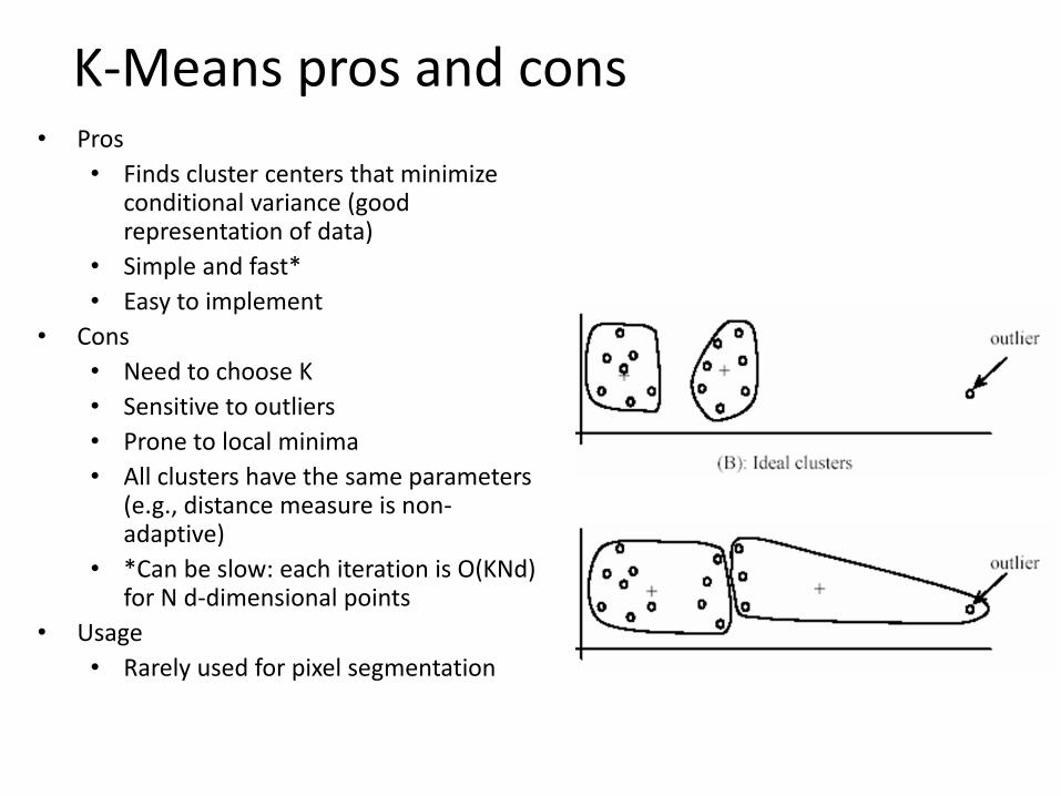
K-Means pros and cons• Pros
• Finds cluster centers that minimize conditional variance (good representation of data)
• Simple and fast*
• Easy to implement
• Cons
• Need to choose K
• Sensitive to outliers
• Prone to local minima
• All clusters have the same parameters (e.g., distance measure is non-adaptive)
• *Can be slow: each iteration is O(KNd) for N d-dimensional points
• Usage
• Rarely used for pixel segmentation

Building Visual Dictionaries
1. Sample patches from a database
– E.g., 128 dimensional SIFT vectors
2. Cluster the patches– Cluster centers are
the dictionary
3. Assign a codeword (number) to each new patch, according to the nearest cluster

Examples of learned codewords
Sivic et al. ICCV 2005http://www.robots.ox.ac.uk/~vgg/publications/papers/sivic05b.pdf
Most likely codewords for 4 learned “topics”
EM with multinomial (problem 3) to get topics

Which algorithm to use?
• Quantization/Summarization: K-means
– Aims to preserve variance of original data
– Can easily assign new point to a cluster
Quantization for
computing histograms
Summary of 20,000 photos of Rome using
“greedy k-means”
http://grail.cs.washington.edu/projects/canonview/

Which algorithm to use?
• Image segmentation: agglomerative clustering
– More flexible with distance measures (e.g., can be based on boundary prediction)
– Adapts better to specific data
– Hierarchy can be useful
http://www.cs.berkeley.edu/~arbelaez/UCM.html


The machine learning
framework
• Apply a prediction function to a feature representation of
the image to get the desired output:
f( ) = “apple”
f( ) = “tomato”
f( ) = “cow”Slide credit: L. Lazebnik

The machine learning
framework
y = f(x)
• Training: given a training set of labeled examples {(x1,y1),
…, (xN,yN)}, estimate the prediction function f by minimizing
the prediction error on the training set
• Testing: apply f to a never before seen test example x and
output the predicted value y = f(x)
output prediction
function
Image
feature
Slide credit: L. Lazebnik

Learning a classifier
Given some set of features with corresponding labels, learn a function to predict the labels from the features
x x
xx
x
x
x
x
oo
o
o
o
x2
x1
Prediction
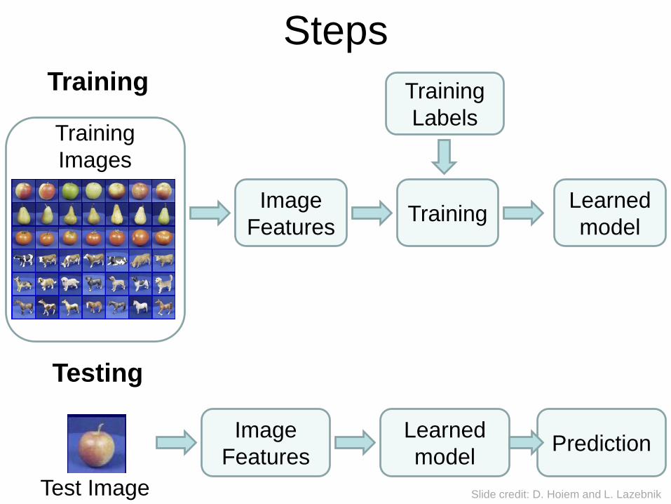
Steps
Training
LabelsTraining
Images
Training
Training
Image
Features
Image
Features
Testing
Test Image
Learned
model
Learned
model
Slide credit: D. Hoiem and L. Lazebnik

Features
• Raw pixels
• Histograms
• GIST descriptors
• …Slide credit: L. Lazebnik
One way to think about it…
• Training labels dictate that two examples are the same or different, in some sense
• Features and distance measures define visual similarity
• Classifiers try to learn weights or parameters for features and distance measures so that visual similarity predicts label similarity

Many classifiers to choose from
• SVM
• Neural networks
• Naïve Bayes
• Bayesian network
• Logistic regression
• Randomized Forests
• Boosted Decision Trees
• K-nearest neighbor
• RBMs
• Deep Convolutional Network
• Etc.
Which is the best one?

Claim:
The decision to use machine learning is more important than the choice of a particular learning method.
*Deep learning seems to be an exception to this, at the moment, probably because it is learning thefeature representation.

Classifiers: Nearest neighbor
f(x) = label of the training example nearest to x
• All we need is a distance function for our inputs
• No training required!
Test
exampleTraining
examples
from class 1
Training
examples
from class 2
Slide credit: L. Lazebnik

Classifiers: Linear
• Find a linear function to separate the classes:
f(x) = sgn(w x + b)
Slide credit: L. Lazebnik

• Images in the training set must be annotated with the
“correct answer” that the model is expected to produce
Contains a motorbike
Recognition task and supervision
Slide credit: L. Lazebnik

Unsupervised “Weakly” supervised Fully supervised
Definition depends on task
Slide credit: L. Lazebnik

Generalization
• How well does a learned model generalize from
the data it was trained on to a new test set?
Training set (labels known) Test set (labels
unknown)
Slide credit: L. Lazebnik
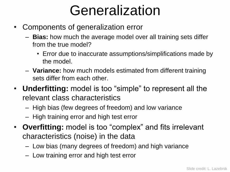
Generalization• Components of generalization error
– Bias: how much the average model over all training sets differ
from the true model?
• Error due to inaccurate assumptions/simplifications made by
the model.
– Variance: how much models estimated from different training
sets differ from each other.
• Underfitting: model is too “simple” to represent all the
relevant class characteristics
– High bias (few degrees of freedom) and low variance
– High training error and high test error
• Overfitting: model is too “complex” and fits irrelevant
characteristics (noise) in the data
– Low bias (many degrees of freedom) and high variance
– Low training error and high test error
Slide credit: L. Lazebnik
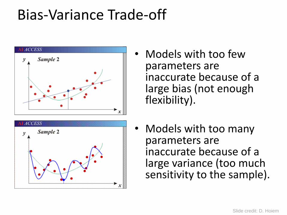
Bias-Variance Trade-off
• Models with too few parameters are inaccurate because of a large bias (not enough flexibility).
• Models with too many parameters are inaccurate because of a large variance (too much sensitivity to the sample).
Slide credit: D. Hoiem

Bias-Variance Trade-off
E(MSE) = noise2 + bias2 + variance
See the following for explanations of bias-variance (also Bishop’s “Neural
Networks” book):
•http://www.inf.ed.ac.uk/teaching/courses/mlsc/Notes/Lecture4/BiasVariance.pdf
Unavoidable
error
Error due to
incorrect
assumptions
Error due to
variance of training
samples
Slide credit: D. Hoiem

Bias-variance tradeoff
Training error
Test error
Underfitting Overfitting
Complexity Low Bias
High Variance
High Bias
Low Variance
Err
or
Slide credit: D. Hoiem

Bias-variance tradeoff
Many training examples
Few training examples
Complexity Low Bias
High Variance
High Bias
Low Variance
Test E
rror
Slide credit: D. Hoiem

Effect of Training Size
Testing
Training
Generalization Error
Number of Training Examples
Err
or
Fixed prediction model
Slide credit: D. Hoiem

Remember…
• No classifier is inherently better than any other: you need to make assumptions to generalize
• Three kinds of error– Inherent: unavoidable
– Bias: due to over-simplifications
– Variance: due to inability to perfectly estimate parameters from limited data
Slide credit: D. Hoiem

How to reduce variance?
• Choose a simpler classifier
• Regularize the parameters
• Get more training data
Slide credit: D. Hoiem

Very brief tour of some classifiers
• K-nearest neighbor
• SVM
• Boosted Decision Trees
• Neural networks
• Naïve Bayes
• Bayesian network
• Logistic regression
• Randomized Forests
• RBMs
• Etc.

Generative vs. Discriminative Classifiers
Generative Models
• Represent both the data and the labels
• Often, makes use of conditional independence and priors
• Examples– Naïve Bayes classifier
– Bayesian network
• Models of data may apply to future prediction problems
Discriminative Models
• Learn to directly predict the labels from the data
• Often, assume a simple boundary (e.g., linear)
• Examples– Logistic regression
– SVM
– Boosted decision trees
• Often easier to predict a label from the data than to model the data
Slide credit: D. Hoiem

Classification
• Assign input vector to one of two or more
classes
• Any decision rule divides input space into
decision regions separated by decision
boundaries
Slide credit: L. Lazebnik

Nearest Neighbor Classifier
• Assign label of nearest training data point to each test data
point
Voronoi partitioning of feature space for two-category 2D and 3D data
from Duda et al.
Source: D. Lowe

K-nearest neighbor
x x
xx
x
x
x
x
o
oo
o
o
o
o
x2
x1
+
+

1-nearest neighbor
x x
xx
x
x
x
x
o
oo
o
o
o
o
x2
x1
+
+
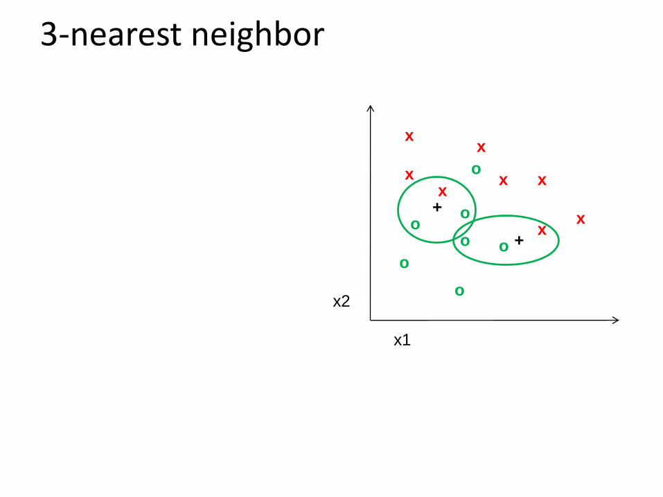
3-nearest neighbor
x x
xx
x
x
x
x
o
oo
o
o
o
o
x2
x1
+
+

5-nearest neighbor
x x
xx
x
x
x
x
o
oo
o
o
o
o
x2
x1
+
+

Using K-NN
• Simple, a good one to try first
• With infinite examples, 1-NN provably has error that is at most twice Bayes optimal error

Classifiers: Linear SVM
x x
xx
x
x
x
x
oo
o
o
o
x2
x1
• Find a linear function to separate the classes:
f(x) = sgn(w x + b)

Classifiers: Linear SVM
x x
xx
x
x
x
x
oo
o
o
o
x2
x1
• Find a linear function to separate the classes:
f(x) = sgn(w x + b)

Classifiers: Linear SVM
x x
xx
x
x
x
x
o
oo
o
o
o
x2
x1
• Find a linear function to separate the classes:
f(x) = sgn(w x + b)

What about multi-class SVMs?
• Unfortunately, there is no “definitive” multi-
class SVM formulation
• In practice, we have to obtain a multi-class
SVM by combining multiple two-class SVMs
• One vs. others• Traning: learn an SVM for each class vs. the others
• Testing: apply each SVM to test example and assign to it the
class of the SVM that returns the highest decision value
• One vs. one• Training: learn an SVM for each pair of classes
• Testing: each learned SVM “votes” for a class to assign to
the test example
Slide credit: L. Lazebnik
SVMs: Pros and cons
• Pros• Many publicly available SVM packages:
http://www.kernel-machines.org/software
• Kernel-based framework is very powerful, flexible
• SVMs work very well in practice, even with very small
training sample sizes
• Cons• No “direct” multi-class SVM, must combine two-class SVMs
• Computation, memory
– During training time, must compute matrix of kernel values for
every pair of examples
– Learning can take a very long time for large-scale problems

What to remember about classifiers
• No free lunch: machine learning algorithms are tools, not dogmas
• Try simple classifiers first
• Better to have smart features and simple classifiers than simple features and smart classifiers
• Use increasingly powerful classifiers with more training data (bias-variance tradeoff)
Slide credit: D. Hoiem

Making decisions about data
• 3 important design decisions:1) What data do I use?
2) How do I represent my data (what feature)?
3) What classifier / regressor / machine learning tool do I use?
• These are in decreasing order of importance
• Deep learning addresses 2 and 3 simultaneously (and blurs the boundary between them).
• You can take the representation from deep learning and use it with any classifier.