
LyX Configuration Manualelibrary.bsi.ac.id/ebook/2016_Deep_Learning_Made_Easy_with_R.pdf · Copies...
253
Ego autem et domus mea serviemus Domino.
Transcript of LyX Configuration Manualelibrary.bsi.ac.id/ebook/2016_Deep_Learning_Made_Easy_with_R.pdf · Copies...

Ego autem et domus
mea serviemus Domino.


DEEP LEARNINGMADE EASY
WITH RA Gentle Introduction for Data Science.
Dr. N.D. Lewis

Copyright © 2016 by N.D. Lewis
All rights reserved. No part of this publication may be reproduced, dis-tributed, or transmitted in any form or by any means, including photo-copying, recording, or other electronic or mechanical methods, withoutthe prior written permission of the author, except in the case of brief quo-tations embodied in critical reviews and certain other noncommercial usespermitted by copyright law. For permission requests, contact the authorat: www.AusCov.com.
Disclaimer: Although the author and publisher have made every effort toensure that the information in this book was correct at press time, theauthor and publisher do not assume and hereby disclaim any liability toany party for any loss, damage, or disruption caused by errors or omissions,whether such errors or omissions result from negligence, accident, or anyother cause.
Ordering Information: Quantity sales. Special discounts are available onquantity purchases by corporations, associations, and others. For details,email: [email protected]
Image photography by Deanna Lewis
ISBN: 978-1519514219ISBN: 1519514212

Contents
Acknowledgements iii
Preface viii
How to Get the Most from this Book 1
1 Introduction 5What is Deep Learning? . . . . . . . . . . . . . . . . . . . . . . . . . . . . . . 6What Problems Can Deep Learning Solve? . . . . . . . . . . . . . . . . . . . 8Who Uses Deep Learning? . . . . . . . . . . . . . . . . . . . . . . . . . . . . . 9A Primer on Neural Networks . . . . . . . . . . . . . . . . . . . . . . . . . . . 11Notes . . . . . . . . . . . . . . . . . . . . . . . . . . . . . . . . . . . . . . . . 24
2 Deep Neural Networks 31The Amazingly Simple Anatomy of the DNN . . . . . . . . . . . . . . . . . . 32How to Explain a DNN in 60 Seconds or Less . . . . . . . . . . . . . . . . . . 33Three Brilliant Ways to Use Deep Neural Networks . . . . . . . . . . . . . . . 34How to Immediately Approximate Any Function . . . . . . . . . . . . . . . . 42The Answer to How Many Neurons to Include . . . . . . . . . . . . . . . . . . 48The ABCs of Choosing the Optimal Number of Layers . . . . . . . . . . . . . 49Three Ideas to Supercharge DNN Performance . . . . . . . . . . . . . . . . . 51Incredibly Simple Ways to Build DNNs with R . . . . . . . . . . . . . . . . . 57Notes . . . . . . . . . . . . . . . . . . . . . . . . . . . . . . . . . . . . . . . . 83
3 Elman Neural Networks 87What is an Elman Neural Network? . . . . . . . . . . . . . . . . . . . . . . . 88What is the Role of Context Layer Neurons? . . . . . . . . . . . . . . . . . . 88How to Understand the Information Flow . . . . . . . . . . . . . . . . . . . . 89How to Use Elman Networks to Boost Your Result’s . . . . . . . . . . . . . . 91Four Smart Ways to use Elman Neural Networks . . . . . . . . . . . . . . . . 92The Easy Way to Build Elman Networks . . . . . . . . . . . . . . . . . . . . 95Here is How to Load the Best Packages . . . . . . . . . . . . . . . . . . . . . 95Why Viewing Data is the New Science . . . . . . . . . . . . . . . . . . . . . . 96The Secret to Transforming Data . . . . . . . . . . . . . . . . . . . . . . . . . 100How to Estimate an Interesting Model . . . . . . . . . . . . . . . . . . . . . . 102Creating the Ideal Prediction . . . . . . . . . . . . . . . . . . . . . . . . . . . 104Notes . . . . . . . . . . . . . . . . . . . . . . . . . . . . . . . . . . . . . . . . 106
i

4 Jordan Neural Networks 107Three Problems Jordan Neural Networks Can Solve . . . . . . . . . . . . . . 108Essential Elements for Effective Jordan Models in R . . . . . . . . . . . . . . 110Which are the Appropriate Packages? . . . . . . . . . . . . . . . . . . . . . . 110A Damn Good Way to Transform Data . . . . . . . . . . . . . . . . . . . . . 112Here is How to Select the Training Sample . . . . . . . . . . . . . . . . . . . . 114Use This Tip to Estimate Your Model . . . . . . . . . . . . . . . . . . . . . . 115Notes . . . . . . . . . . . . . . . . . . . . . . . . . . . . . . . . . . . . . . . . 117
5 The Secret to the Autoencoder 119A Jedi Mind Trick . . . . . . . . . . . . . . . . . . . . . . . . . . . . . . . . . 120The Secret Revealed . . . . . . . . . . . . . . . . . . . . . . . . . . . . . . . . 121A Practical Definition You Can Run With . . . . . . . . . . . . . . . . . . . . 124Saving the Brazilian Cerrado . . . . . . . . . . . . . . . . . . . . . . . . . . . 124The Essential Ingredient You Need to Know . . . . . . . . . . . . . . . . . . . 125The Powerful Benefit of the Sparse Autoencoder . . . . . . . . . . . . . . . . 126Understanding Kullback-Leibler Divergence . . . . . . . . . . . . . . . . . . . 126Three Timeless Lessons from the Sparse Autoencoder . . . . . . . . . . . . . 128Mixing Hollywood, Biometrics & Sparse Autoencoders . . . . . . . . . . . . . 128How to Immediately use the Autoencoder in R . . . . . . . . . . . . . . . . . 131An Idea for Your Own Data Science Projects with R . . . . . . . . . . . . . . 137Notes . . . . . . . . . . . . . . . . . . . . . . . . . . . . . . . . . . . . . . . . 145
6 The Stacked Autoencoder in a Nutshell 147The Deep Learning Guru’s Secret Sauce for Training . . . . . . . . . . . . . 148How Much Sleep Do You Need? . . . . . . . . . . . . . . . . . . . . . . . . . 149Build a Stacked Autoencoder in Less Than 5 Minutes . . . . . . . . . . . . . 153What is a Denoising Autoencoder? . . . . . . . . . . . . . . . . . . . . . . . . 155The Salt and Pepper of Random Masking . . . . . . . . . . . . . . . . . . . . 156The Two Essential Tasks of a Denoising Autoencoder . . . . . . . . . . . . . 156How to Understand Stacked Denoising Autoencoders . . . . . . . . . . . . . . 157A Stunningly Practical Application . . . . . . . . . . . . . . . . . . . . . . . . 158The Fast Path to a Denoising Autoencoder in R . . . . . . . . . . . . . . . . 166Notes . . . . . . . . . . . . . . . . . . . . . . . . . . . . . . . . . . . . . . . . 174
7 Restricted Boltzmann Machines 177The Four Steps to Knowledge . . . . . . . . . . . . . . . . . . . . . . . . . . . 177The Role of Energy and Probability . . . . . . . . . . . . . . . . . . . . . . . 179A Magnificent Way to Think . . . . . . . . . . . . . . . . . . . . . . . . . . . 181The Goal of Model Learning . . . . . . . . . . . . . . . . . . . . . . . . . . . 182Training Tricks that Work Like Magic . . . . . . . . . . . . . . . . . . . . . . 183The Key Criticism of Deep Learning . . . . . . . . . . . . . . . . . . . . . . . 187Two Ideas that can Change the World . . . . . . . . . . . . . . . . . . . . . . 188Secrets to the Restricted Boltzmann Machine in R . . . . . . . . . . . . . . . 194Notes . . . . . . . . . . . . . . . . . . . . . . . . . . . . . . . . . . . . . . . . 201
8 Deep Belief Networks 205How to Train a Deep Belief Network . . . . . . . . . . . . . . . . . . . . . . . 206How to Deliver a Better Call Waiting Experience . . . . . . . . . . . . . . . . 207A World First Idea that You Can Easily Emulate . . . . . . . . . . . . . . . . 209Steps to Building a Deep Belief Network in R . . . . . . . . . . . . . . . . . . 212Notes . . . . . . . . . . . . . . . . . . . . . . . . . . . . . . . . . . . . . . . . 215
Index 222

Dedicated to Angela, wife, friend and mother
extraordinaire.


Acknowledgments
A special thank you to:
My wife Angela, for her patience and constant encouragement.
My daughter Deanna, for taking hundreds of photographs forthis book and my website.
And the readers of my earlier books who contacted me withquestions and suggestions.
iii


Master Deep Learning with this fun,practical, hands on guide.With the explosion of big data deep learning is now on theradar. Large companies such as Google, Microsoft, and Face-book have taken notice, and are actively growing in-house deeplearning teams. Other large corporations are quickly buildingout their own teams. If you want to join the ranks of today’stop data scientists take advantage of this valuable book. It willhelp you get started. It reveals how deep learning models work,and takes you under the hood with an easy to follow processshowing you how to build them faster than you imagined pos-sible using the powerful, free R predictive analytics package.
NO EXPERIENCE REQUIRED - Bestselling decision sci-entist Dr. N.D Lewis builds deep learning models for fun. Nowhe shows you the shortcut up the steep steps to the very top.It’s easier than you think. Through a simple to follow processyou will learn how to build the most successful deep learningmodels used for learning from data. Once you have masteredthe process, it will be easy for you to translate your knowledgeinto your own powerful applications.
If you want to accelerate your progress, discover the best indeep learning and act on what you have learned, this book isthe place to get started.
YOU’LL LEARN HOW TO:
• Develop Recurrent Neural Networks
• Build Elman Neural Networks
• Deploy Jordan Neural Networks
• Create Cascade Correlation Neural Networks
• Understand Deep Neural Networks

Deep Learning Made Easy with R
• Use Autoencoders
• Unleash the power of Stacked Autoencoders
• Leverage the Restricted Boltzmann Machine
• Master Deep Belief Networks
Once people have a chance to learn how deep learning canimpact their data analysis efforts, they want to get hands onwith the tools. This book will help you to start building smarterapplications today using R. Everything you need to get startedis contained within this book. It is your detailed, practical,tactical hands on guide - the ultimate cheat sheet for deeplearning mastery.
A book for everyone interested in machine learning, predic-tive analytic techniques, neural networks and decision science.Buy the book today. Your next big breakthrough using deeplearning is only a page away!
vi

Other Books by N.D Lewis• Build Your Own Neural Network TODAY! Build
neural network models in less time than you ever imag-ined possible. This book contains an easy to follow pro-cess showing you how to build the most successful neuralnetworks used for learning from data using R.
• 92 Applied Predictive Modeling Techniques in R:AT LAST! Predictive analytic methods within easy reachwith R...This jam-packed book takes you under the hoodwith step by step instructions using the popular and freeR predictive analytic package. It provides numerous ex-amples, illustrations and exclusive use of real data to helpyou leverage the power of predictive analytics. A bookfor every data analyst, student and applied researcher.
• 100 Statistical Tests in R: Is designed to give yourapid access to one hundred of the most popular statis-tical tests. It shows you, step by step, how to carry outthese tests in the free and popular R statistical pack-age. The book was created for the applied researcherwhose primary focus is on their subject matter ratherthan mathematical lemmas or statistical theory.
• Visualizing Complex Data Using R: Wish you hadfresh ways to present data, explore relationships, visual-ize your data and break free from mundane charts anddiagrams? In this book you will find innovative ideasto unlock the relationships in your own data and createkiller visuals to help you transform your next presenta-tion from good to great. Visualizing complex relation-ships with ease using R begins here.
For further details visit www.AusCov.com
vii

Deep Learning Made Easy with R
Preface
This is a book for everyone who is interested in deep learn-ing. Deep learning isn’t just for multinational corpo-rations or large university research departments. The
ideas and practical information you’ll find here will work just aswell for the individual data scientist working for a small adver-tising firm, the team of three decision scientists employed by aregional pet foods company, the student completing a projecton deep learning for their coursework, or the solo consultantengaged on a forecasting project for the local health author-ity. You don’t need to be a genius statistician or programmingguru to understand and benefit from the deep learning ideasdiscussed in this text.
The purpose of this book is to introduce deep learning tech-niques to data scientists, applied researchers, hobbyists andothers who would like to use these tools. It is not intended tobe a comprehensive theoretical treatise on the subject. Rather,the intention is to keep the details to the minimum while stillconveying a good idea of what can be done and how to do itusing R. The focus is on the “how” because it is this knowl-edge that will drive innovation and actual practical solutionsfor you. As Anne Isabella Richie, daughter of writer WilliamMakepeace Thackeray, wrote in her novel Mrs. Dymond “...ifyou give a man a fish he is hungry again in an hour. If youteach him to catch a fish you do him a good turn”.
This book came out of the desire to put the powerful tech-nology of deep learning into the hands of the everyday prac-titioner. The material is therefore designed to be used by theindividual whose primary focus is on data analysis and model-ing. The focus is solely on those techniques, ideas and strategiesthat have been proven to work and can be quickly digested anddeployed in the minimal amount of time.
On numerous occasions, individuals in a wide variety ofdisciplines and industries, have asked “how can I quickly un-
viii

derstand and use the techniques of deep learning in my area ofinterest?” The answer used to involve reading complex math-ematical texts and then programming complicated formulas inlanguages such as C, C++ and Java.
With the rise of R, using the techniques of deep learning isnow easier than ever. This book is designed to give you rapidaccess. It shows you, step by step, how to build each typeof deep learning model in the free and popular R statisticalpackage. Examples are clearly described and can be typeddirectly into R as printed on the page.
The least stimulating aspect of the subject for the practi-tioner is the mechanics of calculation. Although many of thehorrors of this topic are necessary for the theoretician, they areof minimal importance to the practitioner and can be elimi-nated almost entirely by the use of the R package. It is in-evitable that a few fragments remain, these are fully discussedin the course of this text. However, as this is a hands on, roleup your sleeves and apply the ideas to real data book, I do notspend much time dealing with the minutiae of algorithmic mat-ters, proving theorems, discussing lemmas or providing proofs.
Those of us who deal with data are primarily interested inextracting meaningful structure. For this reason, it is alwaysa good idea to study how other users and researchers have ap-plied a technique in actual practice. This is primarily becausepractice often differs substantially from the classroom or theo-retical text books. To this end and to accelerate your progress,numerous applications of deep learning use are given through-out this text.
These illustrative applications cover a vast range of disci-plines and are supplemented by the actual case studies whichtake you step by step through the process of building the mod-els using R. I have also provided detailed references for furtherpersonal study in the notes section at the end of each chapter.In keeping with the zeitgeist of R, copies of the vast majorityof applied articles referenced in this text are available for free.
ix

Deep Learning Made Easy with R
New users to R can use this book easily and without anyprior knowledge. This is best achieved by typing in the ex-amples as they are given and reading the comments whichfollow. Copies of R and free tutorial guides for beginnerscan be downloaded at https://www.r-project.org/. If youare totally new to R take a look at the amazing tutorialsat http://cran.r-project.org/other-docs.html; they doa great job introducing R to the novice.
In the end, deep learning isn’t about mathematical lemmasor proving theorems. It’s ultimately about real life, real peo-ple and the application of machine learning algorithms to realworld problems in order to drive useful solutions. No matterwho you are, no matter where you are from, no matter yourbackground or schooling, you have the ability to use the ideasoutlined in this book. With the appropriate software tool, alittle persistence and the right guide, I personally believe deeplearning techniques can be successfully used in the hands ofanyone who has a real interest.
The master painter Vincent van Gough once said “Greatthings are not done by impulse, but by a series of small thingsbrought together.” This instruction book is your step by step,detailed, practical, tactical guide to building and deployingdeep learning models. It is an enlarged, revised, and updatedcollection of my previous works on the subject. I’ve condensedinto this volume the best practical ideas available.
I have found, over and over, that an individual who hasexposure to a broad range of modeling tools and applicationswill run circles around the narrowly focused genius who hasonly been exposed to the tools of their particular discipline.Knowledge of how to build and apply deep learning modelswill add considerably to your own personal toolkit.
Greek philosopher Epicurus once said “I write this not forthe many, but for you; each of us is enough of an audiencefor the other.” Although the ideas in this book reach out tothousands of individuals, I’ve tried to keep Epicurus’s principlein mind–to have each page you read give meaning to just one
x

person - YOU.
A PromiseWhen you are done with this book, you will be able to imple-ment one or more of the ideas I’ve talked about in your ownparticular area of interest. You will be amazed at how quickand easy the techniques are to use and deploy with R. Withonly a few different uses you will soon become a skilled practi-tioner.
I invite you therefore to put what you read in these pagesinto action. To help you do that, I’ve created “12 Resourcesto Supercharge Your Productivity in R”, it is yours forFREE. Simply go to http: // www. AusCov. com and down-load it now. It’s my gift to you. It shares with you 12 of thevery best resources you can use to boost your productivity inR.
Now, it’s your turn!
xi


How to Get the Most from this Book
This is a hands on, role up your sleeves and experimentwith the data and R book. You will get the maximumbenefit by typing in the examples, reading the reference
material and experimenting. By working through the numerousexamples and reading the references, you will broaden yourknowledge, deepen you intuitive understanding and strengthenyour practical skill set.
There are at least two other ways to use this book. You candip into it as an efficient reference tool. Flip to the chapter youneed and quickly see how calculations are carried out in R. Forbest results type in the example given in the text, examine theresults, and then adjust the example to your own data. Alter-natively, browse through the real world examples, illustrations,case studies, tips and notes to stimulate your own ideas.
PRACTITIONER TIP �
If you are using Windows you can easily upgrade tothe latest version of R using the installr package.Enter the following:> install.packages("installr")> installr :: updateR ()
If a package mentioned in the text is not in-stalled on your machine you can download it by typinginstall.packages(“package_name”). For example, to down-load the RSNNS package you would type in the R console:> install.packages("RSNNS")
Once the package is installed, you must call it. You do this bytyping in the R console:> require(RSNNS)
1

Deep Learning Made Easy with R
The RSNNS package is now ready for use. You only need to typethis once, at the start of your R session.
Functions in R often have multiple parameters. In the ex-amples in this text I focus primarily on the key parametersrequired for rapid model development. For information on ad-ditional parameters available in a function type in the R console?function_name. For example, to find out about additionalparameters in the elman function, you would type:?elman
Details of the function and additional parameters will appearin your default web browser. After fitting your model of inter-est you are strongly encouraged to experiment with additionalparameters.
PRACTITIONER TIP �
You should only download packages from CRANusing encrypted HTTPS connections. This pro-vides much higher assurance that the code youare downloading is from a legitimate CRAN mir-ror rather than from another server posing as one.Whilst downloading a package from a HTTPS con-nection you may run into an error message some-thing like:"unable to access index for repositoryhttps://cran.rstudio.com/..."This is particularly common on Windows. The in-ternet2 dll has to be activated on versions beforeR-3.2.2. If you are using an older version of Rbefore downloading a new package enter the fol-lowing:> setInternet2(TRUE)
I have also included the set.seed method in the R code
2

samples throughout this text to assist you in reproducing theresults exactly as they appear on the page.
The R package is available for all the major operating sys-tems. Due to the popularity of Windows, examples in this bookuse the Windows version of R.
PRACTITIONER TIP �
Can’t remember what you typed two hours ago!Don’t worry, neither can I! Provided you are loggedinto the same R session you simply need to type:> history(Inf)
It will return your entire history of entered com-mands for your current session.
You don’t have to wait until you have read the entire bookto incorporate the ideas into your own analysis. You can expe-rience their marvelous potency for yourself almost immediately.You can go straight to the section of interest and immediatelytest, create and exploit it in your own research and analysis.
.
PRACTITIONER TIP �
On 32-bit Windows machines, R can only use upto 3Gb of RAM, regardless of how much you haveinstalled. Use the following to check memory avail-ability:> memory.limit ()
To remove all objects from memory:rm(list=ls())
3

Deep Learning Made Easy with R
As implied by the title, this book is about understandingand then hands on building of deep learning models; more pre-cisely, it is an attempt to give you the tools you need to buildthese models easily and quickly using R. The objective is toprovide you the reader with the necessary tools to do the job,and provide sufficient illustrations to make you think aboutgenuine applications in your own field of interest. I hope theprocess is not only beneficial but enjoyable.
Applying the ideas in this book will transform your datascience practice. If you utilize even one idea from each chapter,you will be far better prepared not just to survive but to excelwhen faced by the challenges and opportunities of the everexpanding deluge of exploitable data.
As you use these models successfully in your own area of ex-pertise, write and let me know. I’d love to hear from you. Con-tact me at [email protected] or visit www.AusCov.com.
Now let’s get started!
4

Chapter 1
Introduction
In God we trust. All others must bring data.W. Edwards Deming
In elementary school, Mrs. Masters my teacher, taught meand my fellow students about perspective. Four studentswere “volunteered” to take part, in what turned out to be
a very interesting experiment. Each volunteer was blindfoldedand directed towards a large model of a donkey. The firststudent was led to the tail, and asked to describe what shefelt. The second student was lead to the leg, and again askedto describe what he felt. The same thing was repeated forthe remaining two students, each led to a different part of thedonkey.
Because no one of the blindfolded students had completeinformation, the descriptions of what they were feeling werewidely inaccurate. We laughed and giggled at the absurdityof the suggestions of our fellow blindfolded students. It wasquite clearly a donkey; how could it be anything else! Once theblindfold was taken off the students, they too laughed. Mrs.Masters was an amazing teacher.
In this chapter I am going to draw a picture of the complete“donkey” for you, so to speak. I’ll give an overview of deeplearning, identify some of the major players, touch on areas
5

Deep Learning Made Easy with R
where it has already been deployed, outline why you shouldadd it to your data science toolkit, and provide a primer onneural networks, the foundation of the deep learning techniqueswe cover in this book.
What is Deep Learning?Deep learning is an area of machine learning that emergedfrom the intersection of neural networks, artificial intelligence,graphical modeling, optimization, pattern recognition and sig-nal processing. The models in this emerging discipline havebeen exulted by sober minded scholars in rigorous academicjournals1 “Deep learning networks are a revolutionary develop-ment of neural networks, and it has been suggested that theycan be utilized to create even more powerful predictors.” Fastercomputer processors, cheaper memory and the deluge of newforms of data allow businesses of all sizes to use deep learningto transform real-time data analysis.
Figure 1.1: The deep learning pyramid
Deep learning is about supervised or unsupervised learn-
6

CHAPTER 1. INTRODUCTION
ing from data using multiple layered machine learning mod-els. The layers in these models consist of multiple stages ofnonlinear data transformations, where features of the data arerepresented at successively higher, more abstract layers.
Figure 1.1 illustrates the deep learning pyramid. At thebase are the two core styles of learning from data, supervisedlearning and unsupervised learning. The core element of non-linear data transformation lies at the center of the pyramid,and at the top, in this book, we consider various types of neu-ral networks.
NOTE... �
There are two basic types of learning used in datascience:
1. Supervised learning: Your training datacontain the known outcomes. The model istrained relative to these outcomes.
2. Unsupervised learning: Your trainingdata does not contain any known outcomes.In this case the algorithm self-discovers rela-tionships in your data.
As we work together through the core ideas involved in deeplearning and useful models using R, the general approach wetake is illustrated in Figure 1.2. Whatever specific machinelearning model you develop, you will always come back to thisbasic diagram. Input data is passed to the model and filteredthrough multiple non-linear layers. The final layer consists ofa classifier which determines which class the object of interestbelongs to.
7

Deep Learning Made Easy with R
Figure 1.2: General deep learning framework
The goal in learning from data is to predict a response vari-able or classify a response variable using a group of given at-tributes. This is somewhat similar to what you might do withlinear regression, where the dependent variable (response) ispredicted by a linear model using a group of independent vari-ables (aka attributes or features). However, traditional linearregression models are not considered deep because they do ap-ply multiple layers of non-linear transformation to the data.
Other popular learning from data techniques such as de-cision trees, random forests and support vector machines, al-though powerful tools2, are not deep. Decision trees and ran-dom forests work with the original input data with no trans-formations or new features generated; whilst support vectormachines are considered shallow because they only consist ofa kernel and a linear transformation. Similarly, single hiddenlayer neural networks are also not considered deep as they con-sist of only one hidden layer3.
What Problems Can Deep LearningSolve?The power of deep learning models comes from their abilityto classify or predict nonlinear data using a modest numberof parallel nonlinear steps4. A deep learning model learns theinput data features hierarchy all the way from raw data inputto the actual classification of the data. Each layer extractsfeatures from the output of the previous layer.
8

CHAPTER 1. INTRODUCTION
Figure 1.3: Feed forward neural network with 2 hidden layers
The deep learning models we consider throughout this textare neural networks with multiple hidden layers. The simplestform of deep neural network, as shown in Figure 1.3, containsat least two layers of hidden neurons, where each additionallayer processes the output from the previous layer as input5.
Deep multi-layer neural networks contain many levels ofnonlinearities which allow them to compactly represent highlynon-linear and/ or highly-varying functions. They are good atidentifying complex patterns in data and have been set workto improve things like computer vision and natural languageprocessing, and to solve unstructured data challenges.
Who Uses Deep Learning?Deep learning technology is being used commercially in thehealth care industry, medical image processing6, natural-language processing and in advertising to improve click throughrates. Microsoft, Google, IBM, Yahoo, Twitter, Baidu, Paypaland Facebook are all exploiting deep learning to understanduser’s preferences so that they can recommend targeted ser-
9

Deep Learning Made Easy with R
vices and products. It is popping up everywhere, it is even onyour smartphone where it underpins voice assisted technology.
NOTE... �
The globally distributed and widely read IEEE7
Spectrum magazine reported8“the demand fordata scientists is exceeding the supply. Theseprofessionals garner high salaries and large stockoption packages...” According to the McKinseyGlobal Institute, the United States alone faces ashortage of 140,000 to 190,000 data scientists withthe appropriate skills9. Whilst the Harvard Busi-ness Review declared data science as the sexiestjob of the 21st century10.
You would be hard pressed to think of an area of commercialactivity where deep learning could not be beneficial. Thinkabout this for five minutes. Write down a list of your bestideas.
Here is a list of areas I came up with:
• Process Modeling and Control11.
• Health Diagnostics12.
• Investment Portfolio Management13.
• Military Target Recognition14.
• Analysis of MRI and X-rays15.
• Credit Rating of individuals by banks and other financialinstitutions16.
• Marketing campaigns17.
• Voice Recognition18.
10

CHAPTER 1. INTRODUCTION
• Forecasting the stock market19.
• Text Searching20.
• Financial Fraud Detection21.
• Optical Character Recognition22.
Richard Socher made his list, found a useful application, andco-founded MetaMind23, an innovative company which special-izes in medical image analysis and automated image recogni-tion. Other data scientists, entrepreneurs, applied researchers,and maybe even you, will soon follow Richard into this increas-ingly lucrative space.
A Primer on Neural NetworksNeural networks have been an integral part of the data scien-tist’s toolkit for over a decade24. Their introduction consider-ably improved the accuracy of predictors, and the gradual re-finement of neural network training methods continues to ben-efit both commerce and scientific research. I first came acrossthem in the spring of 1992 when I was completing a thesis formy Master’s degree in Economics. In the grand old and dustyFoyles bookstore located on Charing Cross Road, I stumbledacross a slim volume called Neural Computing by Russell Bealeand Tom Jackson25. I devoured the book, and decided to builda neural network to predict foreign exchange rate movements.
After several days of coding in GW-BASIC, my neural net-work model was ready to be tested. I fired up my Amstrad2286 computer and let it rip on the data. Three and a halfdays later it delivered the results. The numbers compared wellto a wide variety of time series statistical models, and it out-performed every economic theory of exchange rate movement Iwas able to find. I ditched Economic theory but was hooked onpredictive analytics! I have been building, deploying and toying
11
Deep Learning Made Easy with R
with neural networks and other marvelous predictive analyticmodels ever since.
Neural networks came out of the desire to simulate the phys-iological structure and function of the human brain. Althoughthe desire never quite materialized26 it was soon discovered thatthey were pretty good at classification and prediction tasks27.
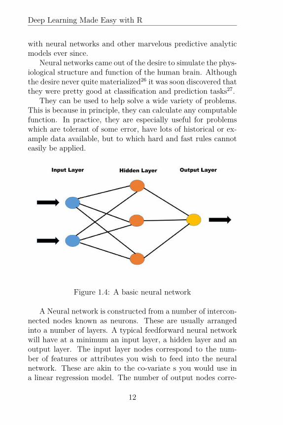
They can be used to help solve a wide variety of problems.This is because in principle, they can calculate any computablefunction. In practice, they are especially useful for problemswhich are tolerant of some error, have lots of historical or ex-ample data available, but to which hard and fast rules cannoteasily be applied.
Figure 1.4: A basic neural network
A Neural network is constructed from a number of intercon-nected nodes known as neurons. These are usually arrangedinto a number of layers. A typical feedforward neural networkwill have at a minimum an input layer, a hidden layer and anoutput layer. The input layer nodes correspond to the num-ber of features or attributes you wish to feed into the neuralnetwork. These are akin to the co-variate s you would use ina linear regression model. The number of output nodes corre-
12

CHAPTER 1. INTRODUCTION
spond to the number of items you wish to predict or classify.The hidden layer nodes are generally used to perform non-lineartransformation on the original input attributes.
privins
school
gender
numchron
health
hosp
Class
Error: 1851.699954 Steps: 16767
Figure 1.5: Multi-Layer Perceptron
In their simplest form, feed-forward neural networks prop-agate attribute information through the network to make aprediction, whose output is either continuous for regression ordiscrete for classification. Figure 1.4 illustrates a typical feedforward neural network topology. It has 2 input nodes, 1 hid-den layer with 3 nodes, and 1 output node. The information isfed forward from the input attributes to the hidden layers and
13

Deep Learning Made Easy with R
then to the output nodes which provide the classification or re-gression prediction. It is called a feed forward neural networkbecause the information flows forward through the network.
Figure 1.5 shows the topology of a typical multi-layer per-ceptron neural network as represented in R. This particularmodel has six input nodes. To the left of each node is thename of the attribute in this case hosp, health, numchron,gender, school and privins respectively. The network hastwo hidden layers, each containing two nodes. The response oroutput variable is called Class. The figure also reports the net-work error, in this case 1851, and the number of steps requiredfor the network to converge.
The Role of the Neuron
Figure 1.6 illustrates the working of a biological neuron. Bi-ological neurons pass signals or messages to each other viaelectrical signals. Neighboring neurons receive these signalsthrough their dendrites. Information flows from the dendritesto the main cell body, known as the soma, and via the axonto the axon terminals. In essence, biological neurons are com-putation machines passing messages between each other aboutvarious biological functions.
At the heart of an artificial neural network is a mathemat-ical node, unit or neuron. It is the basic processing element.The input layer neurons receive incoming information whichthey process via a mathematical function and then distributeto the hidden layer neurons. This information is processedby the hidden layer neurons and passed onto the output layerneurons. The key here is that information is processed viaan activation function. The activation function emulates brainneurons in that they are fired or not depending on the strengthof the input signal.
14

CHAPTER 1. INTRODUCTION
Figure 1.6: Biological Neuron. © Arizona Board of Regents/ ASU Ask A Biologist. https://askabiologist.asu.edu/neuron-anatomy. See also http://creativecommons.org/licenses/by-sa/3.0/
NOTE... �
The original “Perceptron” model was developedat the Cornell Aeronautical Laboratory back in195828. It consisted of three layers with no feed-back:
1. A “retina” that distributed inputs to the sec-ond layer;
2. association units that combine the inputswith weights and a threshold step function;
3. the output layer.
The result of this processing is then weighted and dis-
15

Deep Learning Made Easy with R
tributed to the neurons in the next layer. In essence, neu-rons activate each other via weighted sums. This ensures thestrength of the connection between two neurons is sized accord-ing to the weight of the processed information.
Each neuron contains an activation function and a thresholdvalue. The threshold value is the minimum value that a inputmust have to activate the neuron. The task of the neurontherefore is to perform a weighted sum of input signals andapply an activation function before passing the output to thenext layer.
So, we see that the input layer performs this summation onthe input data. The middle layer neurons perform the sum-mation on the weighted information passed to them from theinput layer neurons; and the output layer neurons perform thesummation on the weighted information passed to them fromthe middle layer neurons.
Figure 1.7: Alternative representation of neuron
Figure 1.7 illustrate the workings of an individual neuron.Given a sample of input attributes {x1,...,xn} a weight wij is as-sociated with each connection into the neuron; and the neuronthen sums all inputs according to:
16

CHAPTER 1. INTRODUCTION
f(u) = ∑ni=1 wijxj + bj
The parameter bj is known as the bias and is similar to theintercept in a linear regression model. It allows the network toshift the activation function “upwards” or “downwards”. Thistype of flexibility is important for successful machine learning29.
Activation FunctionsActivation functions for the hidden layer nodes are needed tointroduce non linearity into the network. The activation func-tion is applied and the output passed to the next neuron(s) inthe network. It is designed to limit the output of the neuron,usually to values between 0 to 1 or -1 to +1. In most casesthe same activation function is used for every neuron in a net-work. Almost any nonlinear function does the job, although forthe backpropagation algorithm it must be differentiable and ithelps if the function is bounded.
The sigmoid function is a popular choice. It is an “S” shapedifferentiable activation function. It is shown in Figure 1.8where parameter c is a constant taking the value 1.5. It is pop-ular partly because it can be easily differentiated and thereforereduces the computational cost during training. It also pro-duces an output between the values 0 and 1 and is given by:
f (u) = 11 + exp (−cu)
There are a wide number of activation functions. Four ofthe most popular include:
• Linear function: In this case:
f(u) = u
• Hyperbolic Tangent function: The hyperbolic tan-gent function produces output in the range −1 to +1.This function shares many properties of the sigmoid func-tion; however, because the output space is broader, it is
17

Deep Learning Made Easy with R
sometimes more efficient for modeling complex nonlinearrelations. The function takes the form:
f(u) = tanh (cu)
• Softmax function: It is common practice to use a soft-max function for the output of a neural network. Doingthis gives us a probability distribution over the k classes:
f(u) =exp
(uT
)∑
k exp(
uT
)where T is the temperature (normally set to 1). Note that usinga higher value for T produces a ’softer’ probability distributionover the k classes. It is typically used with a response variablethat has k alternative unordered classes. It can essentially beviewed as a set of binary nodes whose states are mutually con-strained so that exactly one of the k states has value 1 withthe remainder taking the value 0.
• Rectified linear unit (ReLU): Takes the form:
f(u) = max (0, u)
This activation function has proved popular in deep learningmodels because significant improvements of classification rateshave been reported for speech recognition and computer visiontasks30. It only permits activation if a neurons output is pos-itive; and allows the network to compute much faster than anetwork with sigmoid or hyperbolic tangent activation func-tions because it is simply a max operation. It allows sparsityof the neural network because when initialized randomly ap-proximately half of the neurons in the entire network will beset to zero.There is also a smooth approximation which is sometimes usedbecause it is differentiable:
f(u) = log (1 + exp(u))
18

CHAPTER 1. INTRODUCTION
Figure 1.8: The sigmoid function with c = 1.5
Neural Network LearningTo learn from data a neural network uses a specific learning al-gorithm. There are many learning algorithms, but in general,they all train the network by iteratively modifying the connec-tion weights until the error between the output produced bythe network and the desired output falls below a pre-specifiedthreshold.
The backpropagation algorithm was the first popular lean-ing algorithm and is still widely used. It uses gradient descentas the core learning mechanism. Starting from random weightsthe backpropagation algorithm calculates the network weightsmaking small changes and gradually making adjustments deter-mined by the error between the result produced by the networkand the desired outcome.
The algorithm applies error propagation from outputs toinputs and gradually fine tunes the network weights to min-imize the sum of error using the gradient descent technique.Learning therefore consists of the following steps.
• Step 1:- Initialization of the network: The initial
19

Deep Learning Made Easy with R
values of the weights need to be determined. A neuralnetwork is generally initialized with random weights.
• Step 2:- Feed Forward: Information is passed for-ward through the network from input to hidden andoutput layer via node activation functions and weights.The activation function is (usually) a sigmoidal (i.e.,bounded above and below, but differentiable) functionof a weighted sum of the nodes inputs.
• Step 3:- Error assessment: The output of the networkis assessed relative to known output. If the error is belowa pre-specified threshold the network is trained and thealgorithm terminated.
• Step 4:- Propagate: The error at the output layer isused to re-modify the weights. The algorithm propagatesthe error backwards through the network and computesthe gradient of the change in error with respect to changesin the weight values.
• Step 5:- Adjust: Make adjustments to the weights us-ing the gradients of change with the goal of reducing theerror. The weights and biases of each neuron are adjustedby a factor based on the derivative of the activation func-tion, the differences between the network output and theactual target outcome and the neuron outputs. Throughthis process the network “learns”.
The basic idea is roughly illustrated in Figure 1.9. If the par-tial derivative is negative, the weight is increased (left part ofthe figure); if the partial derivative is positive, the weight isdecreased (right part of the figure)31. Each cycle through thislearning process is called an epoch.
20

CHAPTER 1. INTRODUCTION
Figure 1.9: Basic idea of the backpropagation algorithm
NOTE... �
Neural networks are initialized by setting randomvalues to the weights and biases. One rule ofthumb is to set the random values to lie in therange (-2 n to 2 n), where n is the number of inputattributes.
I discovered early on that backpropagation using gradientdescent often converges very slowly or not at all. In my firstcoded neural network I used the backpropagation algorithmand it took over 3 days for the network to converge to a solution!
Despite the relatively slow learning rate associated withbackpropagation, being a feedforward algorithm, it is quiterapid during the prediction or classification phase.
Finding the globally optimal solution that avoids local min-ima is a challenge. This is because a typical neural networkmay have hundreds of weights whose combined values are usedto generate a solution. The solution is often highly nonlin-
21

Deep Learning Made Easy with R
ear which makes the optimization process complex. To avoidthe network getting trapped in a local minima a momentumparameter is often specified.
Deep learning neural networks are useful in areas whereclassification and/ or prediction is required. Anyone interestedin prediction and classification problems in any area of com-merce, industry or research should have them in their toolkit.In essence, provided you have sufficient historical data or casestudies for which prediction or classification is required you canbuild a neural network model.
Here are four things to try right now:
1. Do an internet search using terms similar to “deep learn-ing jobs”, “machine learning jobs” , "machine learningjobs salary" and "deep learning jobs salary". What dofind?
2. Identify four areas where deep learning could be of per-sonal benefit to you and/ or your organization. Now pickthe area you are most interested in. Keep this topic inmind as you work through the remainder of this book. Ifpossible, go out and collect some data on this area now.By the way, jot down your thoughts in your innovationjournal. Refer back to these as you work through thistext. If you don’t have an innovation/ ideas journal - goout and get one! It will be your personal gold mine fornew and innovative solutions32.
3. If you are new to R, or have not used it in a while, re-fresh your memory by reading the amazing FREE tutori-als at http://cran.r-project.org/other-docs.html.You will be “up to speed” in record time!
4. R- user groups are popping up everywhere. Look for onein you local town or city. Join it! Here are a few resourcesto get you started:
22

CHAPTER 1. INTRODUCTION
• For my fellow Londoners check out: http://www.londonr.org/.
• A global directory is listed at: http://blog.revolutionanalytics.com/local-r-groups.html.
• Another global directory is available at: http://r-users-group.meetup.com/.
• Keep in touch and up to date with useful infor-mation in my FREE newsletter. Sign up at www.AusCov.Com.
23

Deep Learning Made Easy with R
Notes1See Spencer, Matt, Jesse Eickholt, and Jianlin Cheng. "A Deep Learn-
ing Network Approach to ab initio Protein Secondary Structure Predic-tion." Computational Biology and Bioinformatics, IEEE/ACM Transac-tions on 12.1 (2015): 103-112.
2If you want to learn about these, other data science techniques andhow to use them in R, pick up a copy of 92 Applied Predictive Mod-eling Techniques in R, available at www.AusCov.com.
3For more information on building neural networks using R, pick up acopy of the book Build Your Own Neural Network TODAY! fromwww.AusCov.com.
4It also appears deep architectures can be more efficient (in terms ofnumber of fitting parameters) than a shallow network. See for example Y.Bengio, Y. LeCun, et al. Scaling learning algorithms towards ai. Large-scale kernel machines, 34(5), 2007.
5See:
• Hinton G. E., Osindero S., Teh Y. (2006). “A fast learning algo-rithm for deep belief nets”, Neural Computation 18: 1527–1554.
• BengioY (2009) Learning deep architectures for AI, Foundationsand Trends in Machine Learning 2:1–127.
6See for example http://www.ersatzlabs.com/7The IEEE is the world’s largest professional organization devoted to
engineering and the applied sciences. It has over 400,000 members glob-ally.
8See the report by Emily Waltz. Is Data Scientist the Sexiest Jobof Our Time? IEEE Spectrum. September 2012. Also availableat http://spectrum.ieee.org/tech-talk/computing/it/is-data-scientist-the-sexiest-job-of-our-time
9See the special report by James Manyika, Michael Chui, Brad Brown,Jacques Bughin, Richard Dobbs, Charles Roxburgh, Angela Hung By-ers. Big data: The next frontier for innovation, competition, andproductivity. McKinsey Global Institute. May 2011. Also avail-able at http://www.mckinsey.com/insights/business_technology/big_data_the_next_frontier_for_innovation.
10See Davenport, Thomas H., and D. J. Patil. "Data Scientist: TheSexiest Job of the 21st Century-A new breed of professional holds the keyto capitalizing on big data opportunities. But these specialists aren’t easyto find—And the competition for them is fierce." Harvard Business Review(2012): 70.
11See for example:
24
NOTES
1. Shaw, Andre M., Francis J. Doyle, and James S. Schwaber. "Adynamic neural network approach to nonlinear process modeling."Computers & chemical engineering 21.4 (1997): 371-385.
2. Omidvar, Omid, and David L. Elliott. Neural systems for control.Elsevier, 1997.
3. Rivals, Isabelle, and Léon Personnaz. "Nonlinear internal modelcontrol using neural networks: application to processes with delayand design issues." Neural Networks, IEEE Transactions on 11.1(2000): 80-90.
12See for example:
1. Lisboa, Paulo JG. "A review of evidence of health benefit fromartificial neural networks in medical intervention." Neural networks15.1 (2002): 11-39.
2. Baxt, William G. "Application of artificial neural networks to clin-ical medicine." The lancet 346.8983 (1995): 1135-1138.
3. Turkoglu, Ibrahim, Ahmet Arslan, and Erdogan Ilkay. "An intelli-gent system for diagnosis of the heart valve diseases with waveletpacket neural networks." Computers in Biology and Medicine 33.4(2003): 319-331.
13See for example:
1. Khoury, Pascal, and Denise Gorse. "Investing in emerging marketsusing neural networks and particle swarm optimisation." NeuralNetworks (IJCNN), 2015 International Joint Conference on. IEEE,2015.
2. Freitas, Fabio D., Alberto F. De Souza, and Ailson R. de Almeida."Prediction-based portfolio optimization model using neural net-works." Neurocomputing 72.10 (2009): 2155-2170.
3. Vanstone, Bruce, and Gavin Finnie. "An empirical methodologyfor developing stock market trading systems using artificial neuralnetworks." Expert Systems with Applications 36.3 (2009): 6668-6680.
14See for example:
1. Rogers, Steven K., et al. "Neural networks for automatic targetrecognition." Neural networks 8.7 (1995): 1153-1184.
2. Avci, Engin, Ibrahim Turkoglu, and Mustafa Poyraz. "Intelligenttarget recognition based on wavelet packet neural network." ExpertSystems with Applications 29.1 (2005): 175-182.
25

Deep Learning Made Easy with R
3. Shirvaikar, Mukul V., and Mohan M. Trivedi. "A neural networkfilter to detect small targets in high clutter backgrounds." NeuralNetworks, IEEE Transactions on 6.1 (1995): 252-257.
15See for example:
1. Vannucci, A., K. A. Oliveira, and T. Tajima. "Forecast of TEXTplasma disruptions using soft X rays as input signal in a neuralnetwork." Nuclear Fusion 39.2 (1999): 255.
2. Kucian, Karin, et al. "Impaired neural networks for approximatecalculation in dyscalculic children: a functional MRI study." Be-havioral and Brain Functions 2.31 (2006): 1-17.
3. Amartur, S. C., D. Piraino, and Y. Takefuji. "Optimization neuralnetworks for the segmentation of magnetic resonance images." IEEETransactions on Medical Imaging 11.2 (1992): 215-220.
16See for example:
1. Huang, Zan, et al. "Credit rating analysis with support vector ma-chines and neural networks: a market comparative study." Decisionsupport systems 37.4 (2004): 543-558.
2. Atiya, Amir F. "Bankruptcy prediction for credit risk using neu-ral networks: A survey and new results." Neural Networks, IEEETransactions on 12.4 (2001): 929-935.
3. Jensen, Herbert L. "Using neural networks for credit scoring." Man-agerial finance 18.6 (1992): 15-26.
17See for example:
1. Potharst, Rob, Uzay Kaymak, and Wim Pijls. "Neural networks fortarget selection in direct marketing." ERIM report series referenceno. ERS-2001-14-LIS (2001).
2. Vellido, A., P. J. G. Lisboa, and K. Meehan. "Segmentation of theon-line shopping market using neural networks." Expert systemswith applications 17.4 (1999): 303-314.
3. Hill, Shawndra, Foster Provost, and Chris Volinsky. "Network-based marketing: Identifying likely adopters via consumer net-works." Statistical Science (2006): 256-276.
18See for example:
1. Waibel, Alexander, et al. "Phoneme recognition using time-delayneural networks." Acoustics, Speech and Signal Processing, IEEETransactions on 37.3 (1989): 328-339.
26

NOTES
2. Lippmann, Richard P. "Review of neural networks for speech recog-nition." Neural computation 1.1 (1989): 1-38.
3. Nicholson, Joy, Kazuhiko Takahashi, and Ryohei Nakatsu. "Emo-tion recognition in speech using neural networks." Neural comput-ing & applications 9.4 (2000): 290-296.
19See for example:
1. Kimoto, Tatsuya, et al. "Stock market prediction system with mod-ular neural networks." Neural Networks, 1990., 1990 IJCNN Inter-national Joint Conference on. IEEE, 1990.
2. Fernandez-Rodrıguez, Fernando, Christian Gonzalez-Martel, andSimon Sosvilla-Rivero. "On the profitability of technical tradingrules based on artificial neural networks: Evidence from the Madridstock market." Economics letters 69.1 (2000): 89-94.
3. Guresen, Erkam, Gulgun Kayakutlu, and Tugrul U. Daim. "Usingartificial neural network models in stock market index prediction."Expert Systems with Applications 38.8 (2011): 10389-10397.
20See for example:
1. Chung, Yi-Ming, William M. Pottenger, and Bruce R. Schatz. "Au-tomatic subject indexing using an associative neural network." Pro-ceedings of the third ACM conference on Digital libraries. ACM,1998.
2. Frinken, Volkmar, et al. "A novel word spotting method based onrecurrent neural networks." Pattern Analysis and Machine Intelli-gence, IEEE Transactions on 34.2 (2012): 211-224.
3. Zhang, Min-Ling, and Zhi-Hua Zhou. "Multilabel neural networkswith applications to functional genomics and text categorization."Knowledge and Data Engineering, IEEE Transactions on 18.10(2006): 1338-1351.
21See for example:
1. Maes, Sam, et al. "Credit card fraud detection using Bayesianand neural networks." Proceedings of the 1st international naisocongress on neuro fuzzy technologies. 2002.
2. Brause, R., T. Langsdorf, and Michael Hepp. "Neural data miningfor credit card fraud detection." Tools with Artificial Intelligence,1999. Proceedings. 11th IEEE International Conference on. IEEE,1999.
27

Deep Learning Made Easy with R
3. Sharma, Anuj, and Prabin Kumar Panigrahi. "A review of financialaccounting fraud detection based on data mining techniques." arXivpreprint arXiv:1309.3944 (2013).
22See for example:
1. Yu, Qiang, et al. "Application of Precise-Spike-Driven Rule in Spik-ing Neural Networks for Optical Character Recognition." Proceed-ings of the 18th Asia Pacific Symposium on Intelligent and Evo-lutionary Systems-Volume 2. Springer International Publishing,2015.
2. Barve, Sameeksha. "Optical character recognition using artificialneural network." International Journal of Advanced Research inComputer Engineering & Technology 1.4 (2012).
3. Patil, Vijay, and Sanjay Shimpi. "Handwritten English characterrecognition using neural network." Elixir Comp. Sci. & Eng 41(2011): 5587-5591.
23https://www.metamind.io/yours24A historical overview dating back to the 1940’s can be found in Ya-
dav, Neha, Anupam Yadav, and Manoj Kumar. An Introduction to NeuralNetwork Methods for Differential Equations. Dordrecht: Springer Nether-lands, 2015.
25Beale, Russell, and Tom Jackson. Neural Computing-an introduction.CRC Press, 1990.
26Part of the reason is that a artificial neural network might have any-where from a few dozen to a couple hundred neurons. In comparison, thehuman nervous system is believed to have at least 3x10¹⁰neurons.
27When I am talking about a neural network, I should really say "ar-tificial neural network", because that is what we mean most of the time.Biological neural networks are much more complicated in their elemen-tary structures than the mathematical models used in artificial neuralnetworks.
28Rosenblatt, Frank. "The perceptron: a probabilistic model for infor-mation storage and organization in the brain." Psychological review 65.6(1958): 386.
29This is because a multilayer perceptron, say with a step activationfunction, and with n inputs collectively define an n-dimensional space. Insuch a network any given node creates a separating hyperplane producingan "on" output on one side and an "off" output on the other. The weightsdetermine where this hyperplane lies in the input space. Without a biasterm, this separating hyperplane is constrained to pass through the originof the space defined by the inputs. This, in many cases, would severely
28

NOTES
restrict a neural networks ability to learn. Imagine a linear regressionmodel where the intercept is fixed at zero and you will get the picture.
30See for example,
• Wan, L., Zeiler, M., Zhang, S., Cun, Y. L., and Fergus, R. Regu-larization of neural networks using dropconnect. In Proceedings ofthe 30th International Conference on Machine Learning (ICML-13)(2013), pp. 1058–1066.
• Yajie Miao, F. Metze and S. Rawat: Deep maxout networks for low-resource speech recognition. IEEE Workshop on Automatic SpeechRecognition and Understanding (ASRU), 398-403. 2013.
31For a detailed mathematical explanation see, R. Rojas. Neural Net-works. Springer-Verlag, Berlin, 1996
32I like Austin Kleon’s “Steal Like An Artist Journal.” It is anamazing notebook for creative kleptomaniacs. See his website http://austinkleon.com.
29

Deep Learning Made Easy with R
30
Chapter 2
Deep Neural Networks
Data Science is a series of failures punctuated bythe occasional success.N.D Lewis
Remarkable achievements have been made in the prac-tical application of deep learning techniques. Afterdecades of research, many failed applications and the
abandonment of the discipline by all but a few hardcore re-searchers33. What was once thought impossible is now feasibleand deep learning networks have gained immense traction be-cause they have been shown to outperform all other state-of-the-art machine learning tools for a wide variety of applicationssuch as object recognition34, scene understanding35 and occlu-sion detection36.
Deep learning models are being rapidly developed and ap-plied in a wide range of commercial areas due to their supe-rior predictive properties including robustness to overfitting37.They are successfully used in a growing variety of applicationsranging from natural language processing to document recog-nition and traffic sign classification 38.
In this chapter we discuss several practical applications ofthe Deep Neural Network (DNN) ranging from enhancing visi-bility in foggy weather, malware detection and image compres-
31

Deep Learning Made Easy with R
sion. We build a model to investigate the universal approxima-tion theorem, develop a regression style DNN to predict medianhouse prices, create a classification DNN for modeling diabetesand illustrate how to use multiple outputs whilst predictingwaist and hip circumference. During the process you will learnto use a wide variety of R packages, master a few data sciencetricks and pick up a collection of useful tips to enhance DNNperformance.
The Amazingly Simple Anatomy ofDeep Neural NetworksAs illustrated in Figure 2.1, a DNN consists of an input layer,an output layer, and a number of hidden layers sandwiched inbetween the two. It is akin to a multi-layer perceptron (MLP)but with many hidden layers and multiple connected neuronsper layer. The multiple hidden layers of the DNN are advan-tageous because they can approximate extremely complex de-cision functions.
The hidden layers can be considered as increasingly complexfeature transformations. They are connected to the input layersand they combine and weight the input values to produce a newreal valued number, which is then passed to the output layer.The output layer makes a classification or prediction decisionusing the most abstract features computed in the hidden layers.
During DNN learning the weights of the connections be-tween the layers are updated during the training phase in or-der to make the output value as close as possible to the targetoutput. The final DNN solution finds the optimal combinationof weights so that the network function approximates a givendecision function as closely as possible. The network learns thedecision function through implicit examples.
32

CHAPTER 2. DEEP NEURAL NETWORKS
Figure 2.1: A DNN model
How to Explain a DNN in 60 Secondsor LessAs data scientists, we often have to explain the techniques weuse to other data scientists who may be new to the method.Being able to do this is a great skill to acquire. Here is what todo when you absolutely, positively must explain your DNN in60 Seconds or less. Take a deep breath and point to Figure 2.1;the hidden layers are the secret sauce of the DNN. The non-linear data transformations these neurons perform are at theheart of the power of these techniques.
We can view a DNN as a combinations of individual regres-sion models. These models (aka neurons) are chained togetherto provide more flexible combinations of outputs given a set ofinputs than would be possible with a single model. It is thisflexibility that allows them to fit any function. The outputsfrom individual neurons when combined together form the like-lihood of the probable and improbable. The end result beingthe probability of reasonable suspicion that a certain outcome
33

Deep Learning Made Easy with R
belongs to a particular class.Under certain conditions we can interpret each hidden layer
as a simple log-linear model39. The log-linear model is one ofthe specialized cases of generalized linear models for Poisson-distributed data. It is an extension of the two-way contingencyanalysis. Recall from your statistics 101 class, this involvedmeasuring the conditional relationship between two or morediscrete, categorical variables by taking the natural logarithmof cell frequencies within a contingency table. If you took statis-tics 101 and don’t recall this, don’t worry; I also found it hardto stay awake in statistics 101, and I taught the class!
The key take away is that since there are many layers ina typical DNN, the hidden layers can be viewed as a stack oflog-linear models which collectively approximate the posteriorprobability of the response class given the input attributes. Thehidden layers model the posterior probabilities of conditionallyindependent hidden binary neurons given the input attributes.The output layer models the class posterior probabilities.
Three Brilliant Ways to Use DeepNeural NetworksOne of the first hierarchical neural systems was the Neocog-nitron developed in the late 1970’s by the NHK BroadcastingScience Research Laboratories in Tokyo, Japan40. It was aneural network for visual pattern recognition. Although it rep-resented a considerable breakthrough, the technology remainedin the realm of academic research for several decades.
To whet our appetite with more modern applications, let’slook at three practical uses of DNN technology. What youwill recognize from studying these applications is the immensepotential of DNNs in a wide variety of fields. As you readthrough this section, reflect back to your answer to exercise 2on page 22. Ask yourself this question, how can I use DNNsto solve the problems I identified? Read through this section
34

CHAPTER 2. DEEP NEURAL NETWORKS
quickly to stimulate your thinking. Re-read it again at regularintervals. The tools you need to get started will be discussedshortly.
Enhancing Visibility in Foggy WeatherI think we can all agree that visual activities such as objectdetection, recognition, and navigation are much more difficultin foggy conditions. It turns out that faded scene visibility andlower contrast while driving in foggy conditions occurs becauseof the absorption or scattering of light by atmospheric particlessuch as fog, haze, and mist seriously degrades visibility. Sincethe reduction of visibility can dramatically degrade an oper-ator’s judgment in a vehicle and induce erroneous sensing inremote surveillance systems, visibility prediction and enhance-ment methods are of considerable practical value.
In general, de-fogging algorithms require a fogless imageof the same scene41, or salient objects in a foggy image suchas lane markings or traffic signs in order to supply distancecues42. Hanyang University Professor Jechang Jeong and com-puter engineering student Farhan Hussain developed a deepneural network approach to de-fogging images in real time43which works for unseen images. The approach they adopt isquite interesting. They generate an approximate model of thefog composition in a scene using a deep neural network. Detailsof their algorithm are given in Figure 2.2.
Provided the model is not over trained, it turns out thatit can generalize well for de-fogging unseen images. Take alook at Figure 2.3, the top image (a) shows the original scenewithout fog; the middle image (b) the foggy scene; and thebottom image (c) the de-fogged image using the DNN. Hussainand Jeong conclude by stating that “The proposed method isrobust as it achieves good result for a large set of unseen foggyimages.”
35

Deep Learning Made Easy with R
Figure 2.2: Jeong and Hussain’s de-fogging DNN algorithm.Image source Hussain and Jeong cited in endnote item 43..
36

CHAPTER 2. DEEP NEURAL NETWORKS
Figure 2.3: Sample image from Jeong and Hussain’s de-foggingDNN algorithm. Image source Hussain and Jeong cited in end-note item 43.
A Kick in the Goolies for Criminal HackersMalware such as Trojans, worms, spyware, and botnets are ma-licious software which can shut down your computer. Criminalnetworks have exploited these software devices for illegitimategain for as long as there have been uses of the internet.
37

Deep Learning Made Easy with R
A friend, working in the charitable sector, recently foundhis computer shut down completely by such malevolent soft-ware. Not only was the individual unable to access criticalsoftware files or computer programs, the criminals who perpe-trated the attack demanded a significant “ransom” to unlockthe computer system. You may have experienced somethingsimilar.
Fortunately, my friend had a backup, and the ransom wentunpaid. However, the malware cost time, generated worry andseveral days of anxious file recovery. Such attacks impact notonly individuals going about their lawful business, but corpo-rations, and even national governments. Although many ap-proaches have been taken to curb the rise of this malignantactivity it continues to be rampant.
Joshua Saxe and Konstantin Berlin of Invincea Labs, LLC44
use deep neural networks to help identify malicious software45.The DNN architecture consists of an input layer, two hiddenlayers and an output layer. The input layer has 1024 input fea-tures, the hidden layers each have 1024 neurons. Joshua andKonstantin test their model using more than 400,000 softwarebinaries sourced directly from their customers and internal mal-ware repositories.
Now here is the good news. Their DNN achieved a 95%detection rate at 0.1% false positive rate. Wow! But here isthe truly amazing thing, they achieved these results by directlearning on all binaries files, without any filtering, unpacking,or manually separating binary files into categories. This is as-tounding!
What explains their superb results? The researchers ob-serve that “Neural networks also have several properties thatmake them good candidates for malware detection. First, theycan allow incremental learning, thus, not only can they betraining in batches, but they can retrained efficiently (even onan hourly or daily basis), as new training data is collected.Second, they allow us to combine labeled and unlabeled data,through pretraining of individual layers. Third, the classifiers
38
CHAPTER 2. DEEP NEURAL NETWORKS
are very compact, so prediction can be done very quickly usinglow amounts of memory.”
Here is the part you should memorize, internalize and showto your boss when she asks what all this deep learning stuff isabout. It is the only thing that matters in business, research,and for that matter life - results. Joshua and Konstantin con-clude by saying “Our results demonstrate that it is now feasi-ble to quickly train and deploy a low resource, highly accuratemachine learning classification model, with false positive ratesthat approach traditional labor intensive signature based meth-ods, while also detecting previously unseen malware.” And thisis why deep learning matters!
The Incredible Shrinking ImageWay back in my childhood, I watched a movie called “The In-credible Shrinking Man.” It was about a young man, by thename of Scott, who is exposed to a massive cloud of toxic ra-dioactive waste. This was rather unfortunate, as Scott wasenjoying a well deserved relaxing day fishing on his boat.
Rather than killing him outright in a matter of days, assuch exposure might do to me or you; the screen writer usesa little artistic license. The exposure messes with poor Scott’sbiological system in a rather unusual way. You see, withina matter of days Scott begins to shrink. When I say shrink,I don’t mean just his arm, leg or head, as grotesque at thatwould be; Scott’s whole body shrinks in proportion, and hebecomes known as the incredible shrinking man.
Eventually he becomes so small his wife puts him to live ina dolls house. I can tell you, Scott was not a happy camper atthis stage of the movie, and neither would you be. I can’t quiterecall how the movie ends, the last scene I remember involves atiny, minuscule, crumb sized Scott, wielding a steel sowing pinas a sword in a desperate attempt to fend off a vicious lookingspider!
Whilst scientists have not quite solved the problem of how
39

Deep Learning Made Easy with R
to miniaturize a live human, Jeong and Hussain have figuredout how to use a deep neural network to compress images46. Avisual representation of their DNN is shown in Figure 2.4.
Figure 2.4: Jeong and Hussain’s DNN for image compression.Image source Hussain and Jeong cited in endnote item 46.
Notice the model consists of two components - “En-coder”and “Decoder”, this is because image compression con-sists of two phases. In the first phase the image is compressed,and in the second phase it is decompressed to recover the orig-inal image. The number of neurons in the input layer and out-put layer corresponds to the size of image to be compressed.Compression is achieved by specifying a smaller number of neu-rons in the last hidden layer than contained in the originalsinput attribute / output set.
The researches applied their idea to several test images andfor various compression ratios. Rectified linear units were usedfor the activation function in the hidden layers because they“lead to better generalization of the network and reduce the real
40

CHAPTER 2. DEEP NEURAL NETWORKS
compression-decompression time.” Jeong and Hussain also ranthe models using sigmoid activation functions.
Figure 2.5 illustrates the result for three distinct images.The original images are shown in the top panel, the compressedand reconstructed image using the rectified linear units and sig-moid function are shown in the middle and lower panel respec-tively. The researchers observe “The proposed DNN learns thecompression/decompression function very well.” I would agree.What ideas does this give you?
Figure 2.5: Image result of Jeong and Hussain’s DNN for imagecompression. Image source Hussain and Jeong cited in endnoteitem 46
41

Deep Learning Made Easy with R
How to Immediately ApproximateAny FunctionA while back researchers Hornik et al.47 showed that one hid-den layer is sufficient to model any piecewise continuous func-tion. Their theorem is a good one and worth repeating here:
Hornik et al. theorem: Let F be a continu-ous function on a bounded subset of n-dimensionalspace. Then there exists a two-layer neural networkF with a finite number of hidden units that approx-imate F arbitrarily well. Namely, for all x in thedomain of F , |F (x)− F (x) < ε|.
This is a remarkable theorem. Practically, it says that for anycontinuous function F and some error tolerance measured byε, it is possible to build a neural network with one hidden layerthat can calculate F . This suggests, theoretically at least, thatfor very many problems, one hidden layer should be sufficient.
Of course in practice things are a little different. For onething, real world decision functions may not be continuous;the theorem does not specify the number of hidden neuronsrequired. It seems, for very many real world problems manyhidden layers are required for accurate classification and pre-diction. Nevertheless, the theorem holds some practical value.
Let’s build a DNN to approximate a function right nowusing R. First we need to load the required packages. For thisexample, we will use the neuralnet package:> library("neuralnet")
We will build a DNN to approximate y = x2. First wecreate the attribute variable x, and the response variable y.> set.seed (2016)> attribute <- as.data.frame(sample(seq
(-2,2,length =50),50, replace=FALSE),
42

CHAPTER 2. DEEP NEURAL NETWORKS
ncol=1)> response <-attribute ^2
Let’s take a look at the code, line by line. First theset.seed method is used to ensure reproducibility. The sec-ond line generates 50 observations without replacement over therange -2 to +2. The result is stored in the R object attribute.The third line calculates y = x2 with the result stored in the Robject response.
Next we combine the attribute and response objects intoa dataframe called data; this keeps things simple, which isalways a good idea when you are coding in R:> data <- cbind(attribute ,response)> colnames(data) <- c("attribute","response
")
It is a good idea to actually look at your data every nowand then, so let’s take a peek at the first ten observations indata:> head(data ,10)
attribute response1 -1.2653061 1.600999582 -1.4285714 2.040816333 1.2653061 1.600999584 -1.5102041 2.280716375 -0.2857143 0.081632656 -1.5918367 2.533944197 0.2040816 0.041649318 1.1020408 1.214493969 -2.0000000 4.0000000010 -1.8367347 3.37359434
The numbers are as expected with response equal to thesquare of attribute. A visual plot of the simulated data isshown in Figure 2.6.
43

Deep Learning Made Easy with R
Figure 2.6: Plot of y = x2 simulated data
We will fit a DNN with two hidden layers each containingthree neurons. Here is how to do that:> fit<-neuralnet(response~attribute ,data=data ,hidden=c(3,3),threshold =0.01)
The specification of the model formula response~attributefollows standard R practice. Perhaps the only item of interestis threshold which sets the error threshold to be used. Theactual level you set will depend in large part on the application
44

CHAPTER 2. DEEP NEURAL NETWORKS
for which the model is developed. I would image a model usedfor controlling the movements of a scalpel during brain surgerywould require a much smaller error margin than a model devel-oped to track the activity of individual pedestrians in a busyshopping mall. The fitted model is shown in Figure 2.7.
3.79482
2.01092
1.60
144
attribute
1.06787
−1.9
6729
−0.3
9886
−2.89377
−2.16557
−2.8
4845
2.83483.62473
3.47504
3.74
372
6.45553
4.01855
response
1.332613.20961
−2.206
1−0.25719
0.26513
0.44383
1
−1.15031
1
Error: 0.012837 Steps: 3191
Figure 2.7: DNN model for y = x2
Notice that the image shows the weights of the connections andthe intercept or bias weights. Overall, it took 3191 steps forthe model to converge with an error of 0.012837.
Let’s see how good the model really is at approximatinga function using a test sample. We generate 10 observations
45

Deep Learning Made Easy with R
from the range -2 to +2 and store the result in the R objecttestdata:> testdata <- as.matrix(sample(seq(-2,2,
length =10), 10, replace=FALSE), ncol=1)
Prediction in the neuralnet package is achieved using thecompute function:> pred <- compute(fit , testdata)
NOTE... �
To see what attributes are available in any R ob-ject simply type attributes(object_name). Forexample, to see the attributes of pred you wouldtype and see the following:> attributes(pred)$names[1] "neurons" "net.result"
The predicted values are accessed from pred using$net.result. Here is one way to see them:> result <- cbind(testdata ,pred$net.result
,testdata ^2)> colnames(result) <- c("Attribute","
Prediction", "Actual")> round(result ,4)
Attribute Prediction Actual[1,] 2.0000 3.9317 4.0000[2,] -2.0000 3.9675 4.0000[3,] 0.6667 0.4395 0.4444[4,] -0.6667 0.4554 0.4444[5,] 1.5556 2.4521 2.4198
46

CHAPTER 2. DEEP NEURAL NETWORKS
[6,] -1.5556 2.4213 2.4198[7,] -0.2222 0.0364 0.0494[8,] 0.2222 0.0785 0.0494[9,] -1.1111 1.2254 1.2346
[10,] 1.1111 1.2013 1.2346
Figure 2.8: DNN predicted and actual number
The first line combines the DNN prediction(pred$net.result) with the actual observations (testdata^2)into the R object result. The second line gives each columna name (to ease readability when we print to the screen).
47

Deep Learning Made Easy with R
The third line prints the R object result rounding it to fourdecimal places.
The reported numbers indicate the DNN provides a good,although not exact, approximation of the actual function. Thepredicted and fitted values are shown in Figure 2.8. Judge foryourself, what do you think of the DNN models accuracy? Howmight you improve it?
The Answer to How Many Neurons toIncludeAs soon as you begin to see the potential of DNNs the questionof exactly how many neurons to include arises. One way tothink about this issue is to notice that the patterns you wouldlike to extract from your data contain variation. These varia-tions often arise from natural sources (i.e. are randomly drawnfrom a probability distribution) or they may be inherent in theprocess you are trying to model.
In his 1971 work of fiction Wheels, Arthur Hailey explainswhy cars assembled on a Monday or Friday suffer from qualityproblems. Cars produced on Monday were of lower quality dueto the residual effect of weekend drunkenness; whilst cars man-ufactured on Friday suffered from the workers thinking aboutdrunkenness!
In reality, any and every industrial production line will havesome variation. Take for example the production of widgets;although widgets are all created using the same process andmaterials, there will be some variation in weight, size, color andtexture. This variation may not matter for the intended use ofthe widget. However, too much variation between individualwidgets will result in quality issues. In fact, the number of topexecutives who have been fired due to unacceptable variationin the production processes of the widgets they oversee arenumerous48.
The key point is that there will nearly always be some varia-
48

CHAPTER 2. DEEP NEURAL NETWORKS
tion in the patterns you wish to capture from your data. Part ofthis variation will be systematic and can be used to distinguishbetween classes; and part of the variation will be noise whichcannot be used to distinguish between classes. Since differentproblems will have a different mix of systematic variation tonoise induced variation, the optimal number of hidden neuronsis problem specific.
One idea is to use more neurons per layer to detect finerstructure in your data. However, the more hidden neurons usedthe more likely is the risk of over fitting. Over-fitting occursbecause with more neurons there is an increased likelihood thatthe DNN will learn both patterns and noise, rather than theunderlying statistical structure of the data. The result is aDNN which performs extremely well in sample but poorly outof sample.
Here is the key point to keep in mind as you build your DNNmodels. For the best generalization ability, a DNN should haveas few neurons as possible to solve the problem at hand witha tolerable error. The larger the number of training patterns,the larger the number of neurons that can be used whilst stillpreserving the generalization ability of a DNN..
The ABCs of Choosing the OptimalNumber of LayersOne of the major difficulties you will face in building and usingDNNs is the selection of the appropriate number of layers. Theproblem is challenging because it is possible to train a DNNto a very small error on the training sample only to find thatit performs very badly for patterns not used in the trainingprocess.
When this happens to you, and it will, do not be perturbed.The professors who teach the data science classes, books whichoutline the techniques and articles which discuss the latest
49

Deep Learning Made Easy with R
trends rarely reveal this unspoken truth.Pick up any text book and what do you see? Successful
model followed by successful model. Man, by the time I hadfinished my Master’s degree in Statistics, I thought this modelbuilding stuff was a doddle! The funny thing is, year after yearI continue to meet freshly minted Master’s degree students indata science and statistics who think as I once did. You see,the take away for the uninitiated is that the model buildingphase is easy, a breeze, a place where the data scientist canrelax, put their feet up and coast.
In actual practice, data science is a series of failures punc-tuated by the occasional success. If you have spent any timedeploying commercial models, you will inevitably invest a con-siderable amount of time, worry and intellectual capital at themodel development phase.
Unfortunately, with a DNN it is quite possible to have five,six, hell yes even twenty models all performing reasonably wellon the training set! Yet, every single one fail miserably on thetest sample; or worse - your model makes it to production butcrashes in a huge ball of bright flames, illuminating you as itscreator, as it tumbles slowly back to earth. The resultant thickchoking smoke surrounding you and your boss can smootheryour prospects for advancement, stifle opportunity and evenend careers. The selection of the appropriate number of layersis critical.
I think of finding the optimal number of layers as essentiallya model selection problem. It can be partially solved using tra-ditional model selection techniques, one of the most frequentlyused by novices being trial and error, followed by my personalfavorite a systematic global search against selection criteria. Ifyou consider each hidden layer as a feature detector, the morelayers, the more complex feature detectors can be learned. Thisleads to a straightforward rule of thumb, use more layers formore complex functions.
50

CHAPTER 2. DEEP NEURAL NETWORKS
Three Ideas to Supercharge DNN Per-formanceLet’s face it, running neural networks over large datasets re-quires patience. When I coded my very first multi-layer per-ceptron, back in the early 1990’s, I had to wait around threeand a half days per run! And by today’s standards my datasetwas tiny. One of the major problems associated with neuralnetworks in general is the time taken to train networks and thesubsequent problem of the model over-fitting.
Imagine, the situation, the results are needed yesterdayby your boss because your most important client’s campaignis about to launch! Thankfully your large DNN has beentrained over many thousands of connections costing severalhours overnight to a small error. However, when you assessits predictive power on the test sample it fails miserably! Themodel has been over-fit by you! What are you supposed to tellyour boss or worse yet the client? The fact is, as you continueto develop your applied skills in deep learning, you will needsome tricks in your back pocket. Here are three of the best theDNN developer keeps up her sleeve.
Dropout to Enhance SuccessThe image of the derelict who drops out of school, and wastesher life away in the shady recesses of the big city is firmlyimprinted in our culture. Parents warn their children to con-centrate on the lessons, pass the exams and get a good job.Whatever they do, don’t drop out. If you do you will findyourself living in the dark recesses of the big city. When itcomes to going to school, we are advised against dropping outbecause of the fear that it will have a deleterious impact on ourfuture.
The funny thing is, we also celebrate those celebrities andbusiness tycoons who dropped out. These individuals went
51

Deep Learning Made Easy with R
onto enormous success. Heights which would have been impos-sible had they stayed in school! In fact, I cannot think of anarea in industry, education, science, politics or religion whereindividuals who dropped out have not risen to amazing heightsof success. I’d hazard a guess the software or hardware you areusing right now is direct consequence of one such drop out.
Whilst dropping out is both celebrated and derided by ourculture, it appears to also have some upside and downside inrelation to DNNs. Borrowing from the idea that dropping outmight boost DNN performance, suppose we ignore a randomnumber of neurons during each training round49; the processof randomly omitting a fraction of the hidden neurons is calleddropout, see Figure 2.9.
To state this idea a little more formally: for each trainingcase, each hidden neuron is randomly omitted from the net-work with a probability of p. Since the neurons are selected atrandom, different combinations of neurons will be selected foreach training instance.
The idea is very simple and results in a weak learningmodel at each epoch. Weak models have low predictive powerby themselves, however the predictions of many weak modelscan be weighted and combined to produce models with much’stronger’ predictive power.
In fact, dropout is very similar to the idea behind the ma-chine learning technique of bagging50. Bagging is a type ofmodel averaging approach where a majority vote is taken fromclassifiers trained on bootstraped samples of the training data.In fact, you can view dropout as implicit bagging of several neu-ral network models. Dropout can therefore be regarded as anefficient way to perform model averaging across a large numberof different neural networks.
Much of the power of DNNs comes from the fact that eachneuron operates as an independent feature detector. However,in actual practice is common for two or more neurons to be-gin to detect the same feature repeatedly. This is called co-adaptation. It implies the DNN is not utilizing its full capacity
52

CHAPTER 2. DEEP NEURAL NETWORKS
efficiently, in effect wasting computational resources calculat-ing the activation for redundant neurons that are all doing thesame thing.
Figure 2.9: DNN Dropout
In many ways co-adaptation, is similar to the idea ofcollinearity in linear regression, where two or more covariatesare highly correlated. It implies the covariates contain simi-lar information; in particular, that one covariate can be lin-early predicted from the others with a very small error. Inessence, one or more of the covariates are statistically redun-dant. Collinearity can be resolved by dropping one of more ofthe covariates from the model.
Dropout discourages co-adaptations of hidden neurons bydropping out a fixed fraction of the activation of the neurons
53
Deep Learning Made Easy with R
during the feed forward phase of training. Dropout can also beapplied to inputs. In this case, the algorithm randomly ignorecertain inputs.
One of life’s lessons is that dropping out is not necessarilyruinous to future performance, but neither is it a guarantee offuture success, the same is true for dropout in DNNs, there isno absolute guarantee that it will enhance performance, but itis often worth a try. Keep the following three points in mindas you develop your own DNN models:
1. Dropout appears to reduces the likelihood of co-adaptation in noisy samples by creating multiple pathsto correct classification throughout the DNN.
2. The larger the dropout fraction the more noise is intro-duced during training; this slows down learning,
3. It appears to provide the most benefit on very large DNNmodels51.
How to Benefit from Mini BatchingThe traditional backpropagation algorithm, known as batchlearning backpropagation, calculates the change in neuronweights, known as delta’s or gradients, for every neuron in allof the layers of a DNN and for every single epoch. An epoch isone complete forward pass and one backward pass of the errorfor all training examples. The deltas are essentially calculusderivative adjustments designed to minimize the error betweenthe actual output and the DNN output.
A very large DNN might have millions of weights for whichthe delta’s need to be calculated. Think about this for a mo-ment....Millions of weights require gradient calculations.... Asyou might imagine, this entire process can take a considerableamount of time. It is even possible, that the time taken for aDNN to converge on a acceptable solution using batch learning
54

CHAPTER 2. DEEP NEURAL NETWORKS
propagation makes its use in-feasible for a particular applica-tion.
Mini batching is one common approach to speeding up neu-ral network computation. It involves computing the gradienton several training examples at once rather than for each indi-vidual example as happens in the original stochastic gradientdescent algorithm.
A batch consists of a number of training examples in oneforward/backward pass. Note that the larger the batch size,the more memory you will need to run the model. To get asense of the computational efficiency of min-batching, supposeyou had a batch size of 500, with 1000 training examples. Itwill take only 2 iterations to complete 1 epoch.
A common question is when should I use mini batching?The answer really depends on the size of the DNN you arebuilding. The more neurons in the model, the greater the po-tential benefit from mini batching.
Another common question is about the optimal mini batchsize. Although in the text books you often see mini batch sizesof 50, 100, 200 and so on. These are generally for illustrativepurposes. There is a degree of art and science in choosing theoptimal size. In my experience no one number is optimal for allcircumstances. The best advice is to experiment with differentvalues to get a sense of what works for your sample and specificDNN architecture.
A Simple Plan for Early StoppingWhen I was in elementary school we had regular and frequentoutdoor playtime’s as part of our education. We usually hadplaytime mid-morning to whip up our appetite prior to lunch,after lunch to aid the digestive system, and on warm sunnydays, our teachers would unleash us outside for an afternoonplaytime - to burn up any unused energy before we were packedoff home. I loved school!
The only thing that would shorten our frequent outdoor
55

Deep Learning Made Easy with R
adventures was the rain. If it rained (and it rains a lot inEngland) the early stopping bell would ring, the fun would beterminated and the lessons begin. The funny thing was, evenafter a shortened play time my ability to focus and concentrateon my school work was enhanced. I guess my teachers had anintuitive understanding of the link between physical activity,mental focus, mood and performance52. To this day I go outsidefor a brisk walk to jolt my mental faculties into action.
Figure 2.10: Network error by iteration
The analogy with school playtime’s is that we should bewilling to stop DNN training early if that makes it easier to
56

CHAPTER 2. DEEP NEURAL NETWORKS
extract acceptable performance on the testing sample. This isthe idea behind early stopping where the sample is divided intothree sets. A training set, a validation set and a testing set.The test set is used to train the DNN. The training error isusually a monotonic function, that decreases further in everyiteration. Figure 2.10 illustrates this situation. The error fallsrapidly during the first 100 iterations. It then declines at amuch shallower rate over the next three hundred iterations,before leveling off to a constant value.
The validation set is used to monitor the performance ofthe model. The validation error usually falls sharply duringthe early stages as the network rapidly learns the functionalform, but then increases, indicating the model is starting toover fit. In early stopping, training is stopped at the lowesterror achieved on the validation set. The validation model isthen used on the test sample. This procedure has been provento be highly effective in reducing over-fitting for a wide varietyof neural network applications53. It is worth a try by you.
Incredibly Simple Ways to BuildDNNs with RNow we turn our attention to building a DNN model in R usingreal world data. For this example, we will build a regressionDNN to investigate housing values in suburbs of Boston.
A Proven Way to Build Regression DNNsWe begin by loading the packages we will use:> library("neuralnet")> require(Metrics)
We use the functionality of the neuralnet package to buildthe DNN, and the Metrics package to calculate various model
57

Deep Learning Made Easy with R
fit criteria. The dataset used was collected originally by ur-ban planners Harrison and Rubinfeld to generate quantitativeestimates of the willingness of residents to pay for air qualityimprovements in Boston54. It is contained in the MASS package:> data("Boston",package="MASS")> data <-Boston
The R object Boston contains 506 rows and 14 columns.Each column corresponds to a specific variable. Details of eachof the variable used in our analysis are given in Table 1.
Name Descriptioncrim per capita crime rate by town.indus proportion of non-retail business acres per town.nox nitrogen oxides concentration (parts per 10 million).rm average number of rooms per dwelling.age proportion of owner-occupied units built prior to 1940.dis average distances to five Boston employment centres.tax full-value property-tax rate.ptratio pupil-teacher ratio by town.lstat lower status of the population (percent).medv median value of owner-occupied homes.
Table 1: Variables used from Boston data frame.
Here is how to retain only those variable we want to use:> keeps <- c("crim", "indus", "nox", "rm" ,
"age", "dis", "tax" ,"ptratio", "lstat","medv" )
> data <-data[keeps]
The R object data now only contains the variables we are goingto use. The response variable is mdev. Next, we perform aquick check to see if the retained data contains any missingvalues using the apply method:
58

CHAPTER 2. DEEP NEURAL NETWORKS
Great! There are no missing values.The relationship between medv and the explanatory vari-
ables is shown in Figure 2.11.
Figure 2.11: Relationship between medv and other attributes
The next step is to specify the model. I typically use aformula, as I find it an efficient way to write and maintain Rcode. In this case the formula is stored in an R object called
59

Deep Learning Made Easy with R
f. The response variable medv is to be “regressed” against theremaining nine attributes. Here is how to specify it:> f<-medv~ crim + indus + nox + rm + age +
dis + tax + ptratio + lstat
To set up our test sample we use the sample 400 of the 506rows of data without replacement using the sample method:
> set.seed (2016)> n=nrow(data)> train <- sample (1:n, 400, FALSE)
Note the R object train contains the row location of thedata to be used in the test sample. It does not contain theactual observations.
The DNN can be fitted using the neuralnet function. Thiscan be achieved as follows:> fit<- neuralnet(f,data = data[train ,],hidden=c(10 ,12 ,20),algorithm = "rprop+",err.fct = "sse",act.fct = "logistic",threshold =0.1,linear.output=TRUE)
Let’s walk through this statement argument by argument. Thefirst argument (f) contains the model formula. The secondargument specifies the dataset to use (in this case data). Thethird argument is used to indicate how many hidden layersand nodes to include in the model; in this case we specify threehidden layers. The first hidden layer has 10 neurons, the secondhidden layer twelve neurons and the third hidden layer contains20 neurons.The next argument specifies the learning algorithm to be use.Rather than use a traditional backpropagation algorithm Ichoose a more robust version called resilient backpropagation
60

CHAPTER 2. DEEP NEURAL NETWORKS
with backtracking55. This is selected by specifying algorithm= "rprop+". By the way you can use traditional backpropa-gation if you wish by setting algorithm =”backprop”. If youuse this option, you will also need to specify a learning rate(i.e. learningrate =0.01).
The parameter err.fct is the error function; for regres-sion models the sum of squared errors is chosen automatically(err.fct = "sse") . A threshold is set of 0.1 with a logis-tic activation function. Finally, for the output neuron a linearactivation function is selected using linear.output=TRUE.
Prediction using our DNN is straightforward as theneuralnet package has a handy function called compute. Theonly thing we need to do is pass it the DNN model containedin fit along with the test data. Here is how to do that:pred <- compute(fit , data[-train ,1:9])
Notice I pass the row numbers of the test sample by using-train (recall train identified the rows to use in the train-ing sample). Figure 2.12 shows the fitted and predicted valuesalongside the linear regression (solid line). The model appearsto perform reasonably well, although there are a number ofoutlying observations which are not well predicted. This isconfirmed by the performance metrics. I calculate the squaredcorrelation coefficient, mean squared error (mse) and root meansquare error (rmse) for illustration:
round(cor(pred$net.result ,data[-train ,10])^2,6)
[,1][1,] 0.809458
> mse(data [-train ,10], pred$net.result)[1] 0.2607601849
> rmse (data [-train ,10], pred$net.result)[1] 0.5106468299
61

Deep Learning Made Easy with R
Figure 2.12: Predicted and fitted values
The Smart Person’s Tip for DNN RegressionThe great thing about R is that there are multiple packages forestimating neural network models. I always like to build mod-els using a wide variety of packages and learning algorithms.Let’s build a DNN, using traditional backpropagation with thedeepnet package. First let’s load the required package:> require(deepnet)
Next, use the set.seed method for reproducibility, andstore the attributes in the R object X with the response variable
62

CHAPTER 2. DEEP NEURAL NETWORKS
in the R object Y:set.seed (2016)X= data[train ,1:9]Y= data[train ,10]
Here is how to create a DNN:fitB<-nn.train(x=X, y=Y,initW = NULL ,initB = NULL ,hidden = c(10 ,12 ,20),
learningrate = 0.58,momentum =0.74 ,learningrate_scale =1 ,activationfun = "sigm",output = "linear",numepochs = 970,batchsize = 60,hidden_dropout = 0,visible_dropout = 0)
The statement is fairly similar to what we have seen before;however, let’s walk through it line by line. The neural networkis stored in the R object fitB. Notice we pass the attributesand the response variable using the statement x=X, y=Y. Thedeepnet package gives you the ability to specify the startingvalues of the neuron weights (initW) and biases (initB); I setboth values to NULL so that the algorithm will select their valuesat random. The DNN has the same topology as that estimatedon page 60 i.e. three hidden layers, with 10,12 and 20 neuronsin the first, second and third hidden layers respectively.
To use the backpropagation algorithm, you have to spec-ify a learning rate, momentum and learning rate scale56. Thelearning rate controls how quickly or slowly the neural networkconverges. Briefly, momentum involves adding a weighted aver-age of past gradients in the gradient descent updates. It tendsto dampen noise, especially in areas of high curvature of the er-ror function. Momentum can therefore help the network avoid
63

Deep Learning Made Easy with R
becoming trapped in local minima. All three parameters aregenerally set by trial and error, I choose values of 0.58, 0.74and 1 for the learning rate, momentum and learning rate scalerespectively.
The next two lines specify the activation function for thehidden and output neurons. For the hidden neurons I use alogistic function ("sigm"); other options include "linear" or"tanh". For the output neuron I use a linear activation func-tion, other options include "sigm" and "softmax". The modelis run over 970 epochs each with a batch size of 60. No neuronsare dropped out in the input layer or hidden layer.
Prediction using the test sample is similar to what we haveseen before:> Xtest <- data[-train ,1:9]> predB <- nn.predict(fitB , Xtest)
With the performance metrics are calculated as:> round(cor(predB ,data[-train ,10]) ^2,6)
[,1][1,] 0.930665
> mse(data [-train ,10], predB)[1] 0.08525447959
> rmse (data [-train ,10], predB)[1] 0.2919836975
Overall, the process of building a model using the deepnetpackage is fairly similar to the process used with the neuralnetpackage. This is one of the great advantages of using R, pack-ages generally work in similar ways, (although of course theparameters to be specified may be different). Such flexibilityallows you to build similar DNN models rapidly using a vastvariety of different learning algorithms and tuning parameters.
You will find, time and again, that DNNs with the sametopology but different learning algorithms or tuning parameters
64

CHAPTER 2. DEEP NEURAL NETWORKS
will perform on the same underlying data very differently. Theimportant point to remember is that the process of selecting theoptimal DNN model requires selection of a topology, numberof neurons, layers, learning algorithm and tuning parameters.This leads to quite a complex set of combinations! Despitethis, as we have seen, powerful DNN models can be rapidlyconstructed, trained and tested in R. This should lead to aboom in their use in a wide variety of disciplines outside oftheir traditional domain of image, vocal and signal processing.How will you use DNN regression in your next data scienceproject?
The Art of Building Great DNNs for Classi-ficationI would hazard a guess that the vast majority of published ap-plications of DNNs to date involve solving classification prob-lems. The bulk of these applications involve image and signalprocessing. In this section, we look at the application of a DNNmodel to a health related issue. As you work through this casestudy keep your mind open to alternative applications in yourown field of specialized knowledge.
We will build a DNN model using thePimaIndiansDiabetes2 data frame contained in the mlbenchpackage. This dataset was collected by the National Instituteof Diabetes and Digestive and Kidney Diseases57. It contains768 observations on 9 variables measured on females at least21 years old of Pima Indian heritage. Table 2 contains adescription of each variable collected.
The data can be loaded into your R session as follows:> data("PimaIndiansDiabetes2",package="
mlbench")
Let’s do a quick check to ensure we have the expected numberof columns and rows:> ncol(PimaIndiansDiabetes2)
65
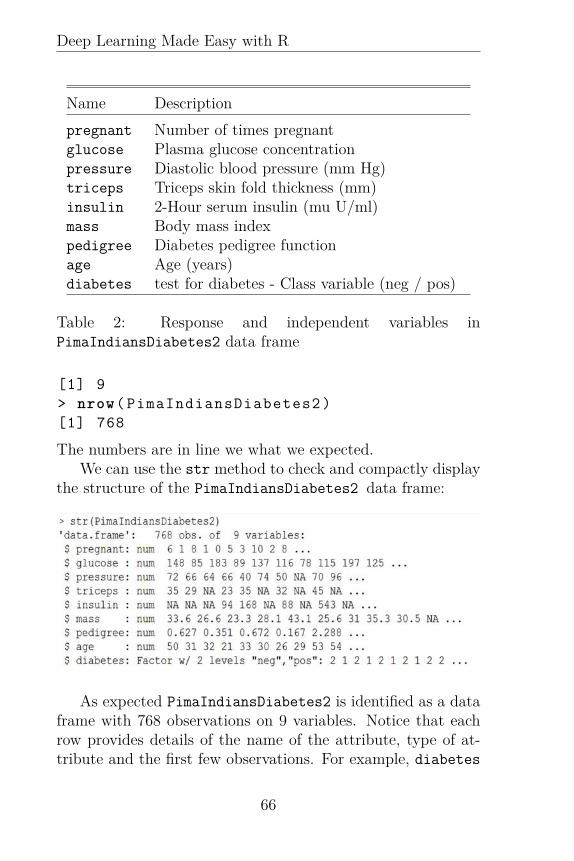
Deep Learning Made Easy with R
Name Descriptionpregnant Number of times pregnantglucose Plasma glucose concentrationpressure Diastolic blood pressure (mm Hg)triceps Triceps skin fold thickness (mm)insulin 2-Hour serum insulin (mu U/ml)mass Body mass indexpedigree Diabetes pedigree functionage Age (years)diabetes test for diabetes - Class variable (neg / pos)
Table 2: Response and independent variables inPimaIndiansDiabetes2 data frame
[1] 9> nrow(PimaIndiansDiabetes2)[1] 768
The numbers are in line we what we expected.We can use the str method to check and compactly display
the structure of the PimaIndiansDiabetes2 data frame:
As expected PimaIndiansDiabetes2 is identified as a dataframe with 768 observations on 9 variables. Notice that eachrow provides details of the name of the attribute, type of at-tribute and the first few observations. For example, diabetes
66

CHAPTER 2. DEEP NEURAL NETWORKS
is a factor with two levels “neg” (negative) and “pos” (posi-tive). We will use it as the classification response variable.
Did you notice the NA values in pressure, triceps,insulin and mass? These are missing values. We all facethe problem of missing data at some point in our work. Peo-ple refuse or forget to answer a question, data is lost or notrecorded properly. It is a fact of data science life! However,there seem to be rather a lot, we better check to see the actualnumbers:
Wow! there are a large number of missing values particu-larly for the attributes of insulin and triceps. How shouldwe deal with this? The most common method and the easiestto apply is to use only those individuals for which we have com-plete information. An alternative is to impute with a plausiblevalue the missing observations. For example, you might replacethe NA’s with the attribute mean or median. A more sophisti-cated approach would be to use a distributional model for thedata (such as maximum likelihood and multiple imputation)58.
Given the large number of missing values in insulin andtriceps we remove these two attributes from the sample anduse the na.omit method to remove any remaining missing val-ues. The cleaned data is stored in temp:> temp<-(PimaIndiansDiabetes2)> temp$insulin <- NULL> temp$triceps <- NULL> temp<-na.omit(temp)
We should have sufficient observations left to do meaningfulanalysis. It is always best to check:> nrow(temp)[1] 724
67
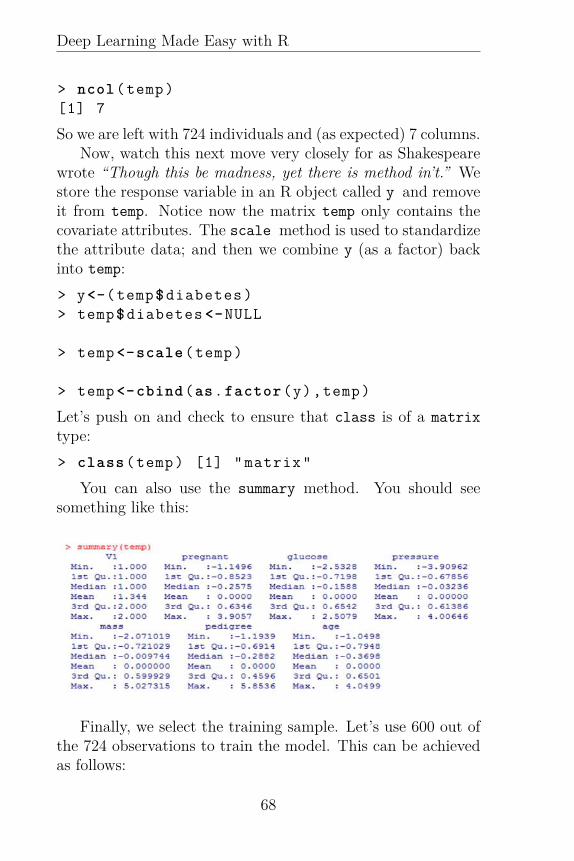
Deep Learning Made Easy with R
> ncol(temp)[1] 7
So we are left with 724 individuals and (as expected) 7 columns.Now, watch this next move very closely for as Shakespeare
wrote “Though this be madness, yet there is method in’t.” Westore the response variable in an R object called y and removeit from temp. Notice now the matrix temp only contains thecovariate attributes. The scale method is used to standardizethe attribute data; and then we combine y (as a factor) backinto temp:> y<-(temp$diabetes)> temp$diabetes <-NULL
> temp<-scale(temp)
> temp<-cbind(as.factor(y),temp)
Let’s push on and check to ensure that class is of a matrixtype:> class(temp) [1] "matrix"
You can also use the summary method. You should seesomething like this:
Finally, we select the training sample. Let’s use 600 out ofthe 724 observations to train the model. This can be achievedas follows:
68

CHAPTER 2. DEEP NEURAL NETWORKS
> set.seed (2016)> n=nrow(temp)
> n_train <- 600> n_test<-n-n_train
> train <- sample (1:n, n_train , FALSE)
To build our DNN we use the RSNNS package:> require(RSNNS)
Keeping things as simple as possible we assign the responsevariable to the R object Y, and the attributes to X:> set.seed (2016)> X<-temp[train ,1:6]> Y<-temp[train ,7]
Now to the meat of the issue, here is how to specify ourclassification DNN in the RSNNS package:fitMLP <- mlp(x=X, y=Y,size = c(12 ,8),maxit = 1000,initFunc = "Randomize_Weights",initFuncParams = c(-0.3, 0.3),learnFunc = "Std_Backpropagation",learnFuncParams = c(0.2, 0),updateFunc = "Topological_Order",updateFuncParams = c(0),hiddenActFunc = "Act_Logistic",shufflePatterns = TRUE ,linOut = TRUE)
Much of this will be familiar to you by now, so I will runthrough it only briefly. The network has two hidden layers;the first hidden layer contains 12 neurons; the second hiddenlayer contains 8 neurons. Weights and biases are initializedrandomly, with a logistic activation function in the hidden lay-ers and linear activation function for the output neuron. You
69

Deep Learning Made Easy with R
will notice, that for this small dataset, the R code executesrelatively quickly.
Prediction is carried out using the predict method. Hereis how I do that for our example:predMLP <- sign(predict(fitMLP , temp[-train
,1:6]))
Since we have classification data, we should take a look at theconfusion matrix. Here it is:> table( predMLP ,sign(temp[-train ,7]) ,dnn =c("Predicted" , " Observed"))
ObservedPredicted -1 1
-1 67 91 21 27
Notice the model did not fit the data perfectly. The offdiagonal elements in the confusion matrix indicate the numberof misclassified observations. It is often helpful to calculate themisclassification as an error rate. Here is how I do that:> error_rate = (1- sum( predMLP == sign(
temp[-train ,7]) )/ 124)> round( error_rate ,3) [1] 0.242
The classification DNN has an overall error rate of around 24%(or an accuracy rate of around 76%).
It is worth highlighting how easily and quickly a classifica-tion DNN can be constructed using R. I can recall spendingmany hours writing code in C++ and C in order to completewhat can now be achieved in a few lines of code in R. If youare interested in the art of data science, that is using the toolsof the discipline to extract meaningful insights, use of R willcertainly boost your productivity.
Asking R users how they build a particular type of model isa bit like the old Econometrician joke:- How many econometri-cians does it take to change a light-bulb? Five, plus or minus
70

CHAPTER 2. DEEP NEURAL NETWORKS
eight! Let’s face it, most of us have our own favorite package,tool and technique. Whilst this is human, a better strategyis to remain flexible, and uncover as many ways as possible tosolve a problem. For R this involves using alternative tools andpackages.
Let’s look at how to build a classification DNN using theAMORE package. (By the way, you could also do this with thepackages we have already used to build a regression DNN. Hav-ing as many arrows in your toolkit is essential to data sciencesuccess.) First, detach the RSNNS package and load AMORE asfollows:> detach("package:RSNNS", unload=TRUE)> library(AMORE)
Here is how to specify a classification DNN in the AMOREpackage:net <- newff(n.neurons=c(6,12,8,1),learning.rate.global =0.01,momentum.global =0.5,error.criterium="LMLS",Stao=NA ,hidden.layer="sigmoid",output.layer="purelin",method="ADAPTgdwm")
Much of this is similar to what you have seen before. Notehowever, that the AMORE package requires you to specify thenumber of input and output nodes as well as hidden nodes.This is achieved using the statement n.neurons=c(6,12,8,1),the first number reflects the six input attributes, the secondand third values represent the number of neurons in the firstand second hidden layers, and the final number the number ofoutput neurons, in this case 1.
Most of the time data scientists train DNNs by minimiz-ing the mean squared error of the training set. However, inthe presence of outliers, the resulting model can struggle to
71
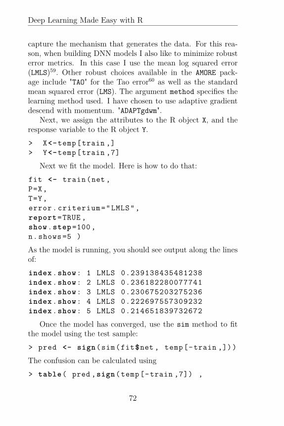
Deep Learning Made Easy with R
capture the mechanism that generates the data. For this rea-son, when building DNN models I also like to minimize robusterror metrics. In this case I use the mean log squared error(LMLS)59. Other robust choices available in the AMORE pack-age include "TAO" for the Tao error60 as well as the standardmean squared error (LMS). The argument method specifies thelearning method used. I have chosen to use adaptive gradientdescend with momentum. "ADAPTgdwm".
Next, we assign the attributes to the R object X, and theresponse variable to the R object Y.> X<-temp[train ,]> Y<-temp[train ,7]
Next we fit the model. Here is how to do that:fit <- train(net ,P=X,T=Y,error.criterium="LMLS",report=TRUE ,show.step=100,n.shows =5 )
As the model is running, you should see output along the linesof:index.show: 1 LMLS 0.239138435481238index.show: 2 LMLS 0.236182280077741index.show: 3 LMLS 0.230675203275236index.show: 4 LMLS 0.222697557309232index.show: 5 LMLS 0.214651839732672
Once the model has converged, use the sim method to fitthe model using the test sample:> pred <- sign(sim(fit$net , temp[-train ,]))
The confusion can be calculated using> table( pred ,sign(temp[-train ,7]) ,
72

CHAPTER 2. DEEP NEURAL NETWORKS
dnn =c("Predicted" ," Observed"))
ObservedPredicted -1 1
-1 71 101 17 26
Finally, the error rate is given by:> error_rate = (1- sum( pred == sign(temp[-
train ,7]) )/ 124)> round( error_rate ,3)[1] 0.218
Overall, the use of adaptive gradient descend with momen-tum learning combined with a robust error resulted in a lowermisclassification error rate of around 22% relative to the clas-sification DNN developed using the RSNNS package. The keytake away here is that as you build your DNN models, do soin a variety of packages, use different learning algorithms, net-work architecture and so on. In other words, at the heart ofthe art of building great DNNs is experimentation.
How to Model Multiple Response Variable’sIn image processing modeling multiple response variables (akapixels) in a single DNN is standard practice. However, in manyareas of data science, models are often built containing only oneresponse variable. This is probably a hangover from the resid-ual dominance of the once ubiquitous linear regression model.
It was probably Sir Francis Galton’s sweet pea experimentback in 187561 which propelled forward the notion of linearregression as a tool for modeling relationships in data. It sub-sequently became the defacto technique of analysis in a widevariety of disciplines. Partly, due to the ease of calculation, the-oretical underpinnings and useful insights, it remains a usefultool to this day.
73

Deep Learning Made Easy with R
A key statistical reason for modeling multiple response vari-ables jointly on the same set of attributes is that it can leadto more efficient parameter estimates62 in regression type mod-els. I first came across the idea of joint estimation of responsevariables several years ago whilst working on surrogate mark-ers in clinical trials. The wonderful thing about this is that thegeneration of more efficient estimates can shorten the durationof clinical trials63. In short, more efficient estimates lead tofaster decisions as the result of greater confidence in terms ofstatistical inference. I can think of multiple instances, across awide range of commercial, industrial and research applications,where modeling multiple response variables on the same set ofattributes is useful. Think for moment about an application inyour line of work. Now let’s look at how to do this in R.
We build our DNN using the data frame bodyfat containedin the TH.data package. The data was originally collected byGarcia et al64 to develop reliable predictive regression equationsfor body fat by measuring skinfold thickness, circumferences,and bone breadth on men and women. The original studycollected data from 117 healthy German subjects, 46 men and71 women. The bodyfat data frame contains the data collectedon 10 variables for the 71 women, see Table 3. Here is how toload the data:> data("bodyfat",package="TH.data")
Waist and hip circumference will serve as the response vari-ables, see Figure 2.13. A visualization of the attributes isshown in Figure 2.14.
74

CHAPTER 2. DEEP NEURAL NETWORKS
Figure 2.13: Kernel density plot for response variables
75

Deep Learning Made Easy with R
Figure 2.14: DNN bodyfat attributes
We will use the neuralnet package to build the DNN. TheMetrics package calculates a variety of useful performancemetrics and is also loaded:> library(neuralnet)> require(Metrics)
Since we are dealing with a rather small dataset, with only71 observations will use 60 observations for the training sample.The data is sampled without replacement as follows:> set.seed (2016)> train <- sample (1:71 ,50 , FALSE)
76

CHAPTER 2. DEEP NEURAL NETWORKS
Name DescriptionDEXfat measure of body fat.age age in years.waistcirc waist circumference.hipcirc hip circumference.elbowbreadth breadth of the elbow.kneebreadth breadth of the knee.anthro3a SLT.anthro3b SLT.anthro3c SLT.anthro4 SLT.
Table 3: Response and independent variables in bodyfat dataframe. Note SLT = sum of logarithm of three anthropometricmeasurements.
Next, the observations are standardized, and the formula to beused to build the DNN is stored in the R object f:> scale_bodyfat <-as.data.frame(scale(log(
bodyfat)))> f<- waistcirc + hipcirc ~ DEXfat+age +
elbowbreadth + kneebreadth + anthro3a +anthro3b + anthro3c +anthro4
Notice the use of waistcirc + hipcirc ~ to indicate tworesponse variables. In general, for k response variables{r1,...,rk} you would use r1+r2+...+rk~.
I fit a model with two hidden layers with 8 neurons in thefirst hidden layer and 4 neurons in the second hidden layer.The remaining parameters are similar to those we have alreadydiscussed:it<- neuralnet(f,data = scale_bodyfat[train ,],hidden=c(8,4),threshold =0.1,
77

Deep Learning Made Easy with R
err.fct = "sse",algorithm = "rprop+",act.fct = "logistic",linear.output=FALSE)
A visualization of the fitted model is shown in Figure 2.15. Themodel only took 45 steps to converge with a sum of squarederrors equal to 25.18.
Now a little bit of housekeeping, I copy the data inscale_bodyfat and store it in the R object without_fat. Thisis the object we will play with. It also allows us to preservethe original values contained in scale_bodyfat which we willuse later. Notice that I also remove the response variables fromthis new R object using the NULL argument:> without_fat<-scale_bodyfat> without_fat$waistcirc <-NULL> without_fat$hipcirc <-NULL
Now we are ready to use the model on the test sample.The approach is similar to that which we have seen before.The second line prints out the predicted values (first few onlyshown):> pred <- compute(fit , without_fat[-train ,]
)> pred$net.resultpred$net.result
[,1] [,2]48 0.8324509945946 0.711776567062753 0.1464097674972 0.038952075658658 0.7197107887754 0.621509147934962 0.8886019185711 0.8420724129305
That’s it! The DNN with two response variables has been suc-cessfully built.
78

CHAPTER 2. DEEP NEURAL NETWORKS
anthro4
anthro3c
anthro3b
anthro3a
kneebreadth
elbowbreadth
age
DEXfat
hipcirc
waistcirc
Error: 25.186069 Steps: 45
Figure 2.15: DNN model with two outputs
Hey, after all of that we may as well compare our 21st cen-tury model results to Sir Francis Galton’s 19th century linearregression model. This will involve building two models. Onefor each of the response variables. First, create the formulas:> fw<- waistcirc ~ DEXfat+age +
elbowbreadth + kneebreadth + anthro3a +anthro3b + anthro3c +anthro4
> fh<- hipcirc ~ DEXfat+age + elbowbreadth+ kneebreadth + anthro3a + anthro3b +
anthro3c +anthro4
79

Deep Learning Made Easy with R
Now run each of the models using the training data:> regw<-linReg <-lm(fw ,data = scale_bodyfat[
train ,])> regh<-linReg <-lm(fh ,data = scale_bodyfat[
train ,])
Next, build predictions using the test sample:> predw <-predict(regw , without_fat[-train
,])> predh <-predict(regh , without_fat[-train
,])
Wow, that was pretty fast! So how does our DNN modelcompare with the linear regressions? The mean squared errorstatistic for the DNN model response variable waistcirc canbe calculated as follows:> mse(scale_bodyfat [-train ,10], pred$net
.result [,1])[1] 0.5376666652
And for Galton’s regression model:> mse(scale_bodyfat [-train ,10], predw)[1] 0.3670629158
Galton’s 19th century linear regression for waist size beats thepants off our deep learning model!What about hip size? Here is the metric for the DNN:> mse(scale_bodyfat [-train ,10], pred$net.
result [,2])[1] 0.5530302859
And for Galton’s hip size regression model:> mse(scale_bodyfat [-train ,10], predh)0.5229634116
A much closer race here, but the linear regression still winswith a smaller mean squared error.
80

CHAPTER 2. DEEP NEURAL NETWORKS
Of course, in practice you will build a variety of models us-ing different learning algorithms, number of neurons and so on;and the linear regression model results serve as a useful bench-mark. To illustrate this point, I build a DNN using traditionalbackpropagation with the deepnet package.
First, I collect the attributes into the R object X, and theresponse variables into the R object Y:> set.seed (2016)> X= as.matrix(without_fat[train ,])> Y= as.matrix(scale_bodyfat[train ,3:4])
The DNN model with 2 hidden layers is estimated as follows:fitB<-nn.train(x=X, y=Y,initW = NULL ,initB = NULL ,hidden = c(8,4),activationfun = "sigm",
learningrate = 0.02,momentum =0.74 ,learningrate_scale =1 ,output = "linear",numepochs = 970,batchsize = 60,hidden_dropout = 0,visible_dropout = 0)
The predicted values, using the test sample, are stored in theR object predB:> Xtest <- as.matrix(without_fat[-train ,])> predB <- nn.predict(fitB , Xtest)
And the mean square error for waistcirc, and hipcirc arecalculated as:> mse(scale_bodyfat [-train ,10], predB
[,1])[1] 0.1443659185
81
Deep Learning Made Easy with R
> mse(scale_bodyfat [-train ,10], predB[,2])
[1] 0.1409938484
In this case, the DNN model outperforms (in terms of meansquare error) the linear regression models.
The key takeaway is not that any particular approach isabsolutely inferior, rather that the data science tool you useshould be selected in order to fit the nature of the problemyou have at hand. As novelist Stephen King wrote65 “It’s bestto have your tools with you. If you don’t, you’re apt to findsomething you didn’t expect and get discouraged.”
82

NOTES
Notes33If you are interested in the history of deep learning see the interest-
ing article at http://recode.net/2015/07/15/ai-conspiracy-the-scientists-behind-deep-learning/
34Krizhevsky, Alex, Ilya Sutskever, and Geoffrey E. Hinton. "Imagenetclassification with deep convolutional neural networks." Advances in neuralinformation processing systems. 2012.
35Couprie, Camille, et al. "Indoor semantic segmentation using depthinformation." arXiv preprint arXiv:1301.3572 (2013).
36Sarkar, Soumik, et al. "Occlusion Edge Detection in RGB-D Framesusing Deep Convolutional Networks." arXiv preprint arXiv:1412.7007(2014).
37For a successful application in image recognition see A. Krizhevsky,I. Sutskever, and G. E. Hinton. Imagenet classication with deep convo-lutional neural networks. In Advances in neural information processingsystems, pages 1097{1105, 2012.
38See for example:1. Keshmiri, Soheil, et al. "Application of Deep Neural Network
in Estimation of the Weld Bead Parameters." arXiv preprintarXiv:1502.04187 (2015).
2. Dahl, George E., et al. "Context-dependent pre-trained deep neuralnetworks for large-vocabulary speech recognition." Audio, Speech,and Language Processing, IEEE Transactions on 20.1 (2012): 30-42.
3. R. Collobert and J. Weston, A unified architecture for natural lan-guage processing: Deep neural networks with multitask learning,in Int. Conf. Machine Learning, 2008.
4. D. C. Ciresan, U. Meier, J. Masci, and J. Schmidhuber, Multi-column deep neural network for traffic sign classification, NeuralNetworks, vol. 32, pp. 333-338, 2012.
5. Y.LeCun, L.Bottou, and P.Haffiner, Gradient-based learning ap-plied document recognition, Proc. of the IEEE, vol.86, pp.2278-2324, 1998.
39For further details see Seide, Frank, et al. "Feature engineering incontext-dependent deep neural networks for conversational speech tran-scription." Automatic Speech Recognition and Understanding (ASRU),2011 IEEE Workshop on. IEEE, 2011.
40Fukushima, Kunihiko. "Neocognitron: A self-organizing neural net-work model for a mechanism of pattern recognition unaffected by shift inposition." Biological cybernetics 36.4 (1980): 193-202.
83

Deep Learning Made Easy with R
41See for example Narasimhan, Srinivasa G., and Shree K. Nayar. "Con-trast restoration of weather degraded images." Pattern Analysis and Ma-chine Intelligence, IEEE Transactions on 25.6 (2003): 713-724.
42Pomerleau, Dean. "Visibility estimation from a moving vehicle usingthe RALPH vision system." IEEE Conference on Intelligent Transporta-tion Systems. 1997.
43Farhan Hussain and Jechang Jeong, “Visibility Enhancement of SceneImages Degraded by Foggy Weather Conditions with Deep Neural Net-works,” Journal of Sensors, vol. 2016, Article ID 3894832, 9 pages, 2016.doi:10.1155/2016/3894832
44Invincea Labs provides an advanced endpoint security solutions thatprevents targeted attacks, detects breaches & supports threat response byeradicating malware.
45Saxe, Joshua, and Konstantin Berlin. "Deep Neural Network BasedMalware Detection Using Two Dimensional Binary Program Features."arXiv preprint arXiv:1508.03096 (2015).
46See Farhan Hussain and Jechang Jeong, “Efficient Deep Neural Net-work for Digital Image Compression Employing Rectified Linear Neu-rons,” Journal of Sensors, vol. 2016, Article ID 3184840, 7 pages, 2016.doi:10.1155/2016/3184840
47See Hornik, M. Stichcombe, and H. White. Multilayer feedforwardnetworks are universal approximators. Neural Networks, 2:359–366, 1989.
48In any year you will find many examples. Here are a couple, fromseveral years ago, to give you a sense of the real world importance of thisissue:
• In November 2013 autoblog reported that Kwon Moon-sik,research and development president of the car manufac-turer Hyundai, resigned as a result of a series of qual-ity issues. See http://www.autoblog.com/2013/11/12/hyundai-executive-resigns-quality-issues/. See alsothe Reuters report at http://www.reuters.com/article/us-hyundai-rd-idUSBRE9AA0F920131111.
• Towards the end of 2014 Fiat Chrysler’s quality chief, Doug Betts,left the company, one day after the automaker ranked last in aclosely watched U.S. scorecard on vehicle reliability. See Automo-tive News article”Betts leaves Chrysler after another poor qualityshowing” by Larry P. Vellequette.
49See:
• Srivastava, Nitish, et al. "Dropout: A simple way to prevent neu-ral networks from overfitting." The Journal of Machine LearningResearch 15.1 (2014): 1929-1958.
84

NOTES
• Hinton, Geoffrey E., et al. "Improving neural networks bypreventing co-adaptation of feature detectors." arXiv preprintarXiv:1207.0580 (2012).
50The idea was proposed by Leo Breiman, who called it "bootstrapaggregating" see Breiman, Leo. "Bagging predictors." Machine learning24.2 (1996): 123-140.
51See for example Dahl, George E., Tara N. Sainath, and Geoffrey E.Hinton. "Improving deep neural networks for LVCSR using rectified linearunits and dropout." Acoustics, Speech and Signal Processing (ICASSP),2013 IEEE International Conference on. IEEE, 2013.
52The link appears to have been validated by a large number of studies.See for example Sharma A, Madaan V, Petty FD. Exercise for MentalHealth. Primary Care Companion to The Journal of Clinical Psychiatry.2006;8(2):106.
53Here are three examples in totally different areas of application :
• Payan, Adrien, and Giovanni Montana. "Predicting Alzheimer’sdisease: a neuroimaging study with 3D convolutional neural net-works." arXiv preprint arXiv:1502.02506 (2015).
• Oko, Eni, Meihong Wang, and Jie Zhang. "Neural network ap-proach for predicting drum pressure and level in coal-fired subcrit-ical power plant." Fuel 151 (2015): 139-145.
• Torre, A., et al. "Prediction of compression strength of high perfor-mance concrete using artificial neural networks." Journal of Physics:Conference Series. Vol. 582. No. 1. IOP Publishing, 2015.
54Harrison, David, and Daniel L. Rubinfeld. "Hedonic housing pricesand the demand for clean air." Journal of environmental economics andmanagement 5.1 (1978): 81-102.
55For additional details on resilient backpropagation see:
• Riedmiller M. (1994) Rprop - Description and Implementation De-tails. Technical Report. University of Karlsruhe.
• Riedmiller M. and Braun H. (1993) A direct adaptive method forfaster backpropagation learning: The RPROP algorithm. Pro-ceedings of the IEEE International Conference on Neural Networks(ICNN), pages 586-591. San Francisco.
56See my book Build Your Own Neural Network TODAY! for aquick and easy explanation of these terms.
57See http://www.niddk.nih.gov/58For alternative approaches to dealing with missing values see:
85

Deep Learning Made Easy with R
1. Roth, Philip L. "Missing data: A conceptual review for appliedpsychologists." Personnel psychology 47.3 (1994): 537-560.
2. Afifi, A. A., and R. M. Elashoff. "Missing observations in multivari-ate statistics I. Review of the literature." Journal of the AmericanStatistical Association 61.315 (1966): 595-604.
3. Pigott, Therese D. "A review of methods for missing data." Educa-tional research and evaluation 7.4 (2001): 353-383.
4. Little, Roderick J., et al. "The prevention and treatment of missingdata in clinical trials." New England Journal of Medicine 367.14(2012): 1355-1360.
59See Liano, Kadir. "Robust error measure for supervised neural net-work learning with outliers." Neural Networks, IEEE Transactions on 7.1(1996): 246-250.
60See for example:
• Pernía-Espinoza, Alpha V., et al. "TAO-robust backpropagationlearning algorithm." Neural Networks 18.2 (2005): 191-204.
• Ordieres-Meré, Joaquín B., Francisco J. Martínez-de-Pisón, andAna González-Marcos. "TAO-robust backpropagation learning al-gorithm." Neural networks 18.2 (2005): 191-204.
• Rusiecki, Andrzej. "Robust LTS backpropagation learning algo-rithm." Computational and ambient intelligence. Springer BerlinHeidelberg, 2007. 102-109.
61See Stanton, Jeffrey M. "Galton, Pearson, and the peas: A brief his-tory of linear regression for statistics instructors." Journal of StatisticsEducation 9.3 (2001).
62See for example Zellner, Arnold, and Tong Hun Lee. "Joint estima-tion of relationships involving discrete random variables." Econometrica:Journal of the Econometric Society (1965): 382-394.
63See for example N.D. Lewis. Surrogate Markers in Clinical Trials.PhD Thesis. University of Cambridge
64Garcia, Ada L., et al. "Improved prediction of body fat by measuringskinfold thickness, circumferences, and bone breadths." Obesity Research13.3 (2005): 626-634.
65See King, Stephen. "On writing: A memoir of the craft." New York:Scribner (2000). If you have not already done so, go out and purchasea copy of this book at your earliest convenience. It is jam packed full ofadvice that will serve you well.
86

Chapter 3
Elman Neural Networks
All models are wrong, but some are useful.George E. P. Box
The Elman neural network is a recurrent neural network.In a recurrent neural network neurons connect back toother neurons, information flow is multi-directional so
the activation of neurons can flow around in a loop. This typeof neural network has a sense of time and memory of earliernetworks states which enables it to learn sequences which varyover time, perform classification tasks and develop predictionsof future states. As a result, recurrent neural networks are usedfor classification, stochastic sequence modeling and associativememory tasks.
A simple form of recurrent neural network is illustrated inFigure 3.1. A delay neuron is introduced in the context layer.It has a memory in the sense that it stores the activation valuesof an earlier time step. It releases these values back into thenetwork at the next time step.
87

Deep Learning Made Easy with R
Figure 3.1: Simple recurrent neural network
What is an Elman Neural Network?Elman neural networks are akin to the multi-layer perceptronaugmented with one or more context layers. The number ofneurons in the context layer is equal to the number of neuronsin the hidden layer. In addition, the context layer neurons arefully connected to all the neurons in the hidden layer.
To solidify this idea let’s take a look at the Elman networkdeveloped by Khatib et al.66 to predict hourly solar radiation.The network is illustrated in Figure 3.2. It is a 3-layered net-work with eight input attributes (Latitude, Longitude, Tem-perature, Sunshine ratio, Humidity, Month, Day, Hour); fivehidden neurons, five context neurons; and two output neuronspredicting global solar radiation and diffused solar radiation.
What is the Role of Context LayerNeurons?The neurons in the context layer are included because theyremember the previous internal state of the network by stor-ing hidden layer neuron values. The stored values are delayedby one time step; and are used during the next time step asadditional inputs to the network.
88

CHAPTER 3. ELMAN NEURAL NETWORKS
Figure 3.2: Schematic illustration of the Elman network topredict hourly solar radiation. Source Khatib et al. cited inendnote sec. 66
How to Understand the InformationFlowTo help strengthen our intuition about this useful model let’slook at a simplified illustration. Suppose we have a neural net-work consisting of only two neurons, as illustrated in Figure 3.3.The network has one neuron in each layer. Each neuron has abias denoted by b1 for the first neuron, and b2 for the secondneuron. The associated weights are w1 and w2 with activation
89

Deep Learning Made Easy with R
function f1 and f2. Since there are only two neurons the outputY as a function of the input attribute X is given by:
Y = f2 (w2f1 (w1X + b1) + b2)
Figure 3.3: Two neuron network
In an Elman network, as shown in Figure 3.4, there is acontext neuron which feeds the signal from the hidden layerneuron67 back to that same neuron. The signal from the contextneuron is delayed by one time step and multiplied by w2 beforebeing fed back into the network. The output at time t is givenby:
Y [t] = f2 (w3f1 (w1X[t] + w2C + b1) + b2)
where,
C = Y1[t− 1]
During the training process the weights and biases are iter-atively adjusted to minimize the network error, typically mea-sured using the mean squared error. If the error is insufficientlysmall another iteration or epoch is initiated. We see, in thissimple example, that the hidden layer is fully connected to in-puts and the network exhibits recurrent connections; and theuse of delayed memory creates a more dynamic neural networksystem.
90

CHAPTER 3. ELMAN NEURAL NETWORKS
Figure 3.4: Two node Elman network
How to Use Elman Networks to BoostYour Result’sElman Neural Networks are useful in applications where weare interested in predicting the next output in given sequence.Their dynamic nature can capture time-dependent patterns,which are important for many practical applications. This typeof flexibility is important in the analysis of time series data.
A typical example is the Elman network, shown inFigure 3.2 to predict hourly solar radiation developed byKhatib et al. The property of memory retention is also use-ful for pattern recognition and robot control.
91

Deep Learning Made Easy with R
Four Smart Ways to use Elman NeuralNetworksLet’s take a look at some interesting applications of Elmanneural networks. The applications range from fault prediction,weather forecasting to predicting the stock market. In eachillustration discussed below, the power of this predictive toolbecomes evident. Take a look, then answer the question ofhow will you apply this incredible tool in your data modelingchallenges?
The Ultimate Weather Forecasting ModelAccurate weather forecasts are of keen interest to all sectionsof society. Farmers look to weather conditions to guide theplanting and harvesting of their crops, transportation authori-ties seek information on the weather to determine whether toclose or open specific transportation corridors, and individualsmonitor the weather as they go about their daily activities.
Maqsood, Khan and Abraham68 develop a Elman neu-ral network to forecast the weather of Vancouver, BritishColumbia, Canada. They specifically focus on creating mod-els to forecast the daily maximum temperature, minimum dailytemperature and wind-speed. The dataset consisted of one yearof daily observations. The first eleven months were used totrain the network with the testing set consisting of the finalmonth’s data (1st to 31st August). The optimal model had 45hidden neurons with Tan-sigmoid activation functions.
The peak temperature forecast had an average correlationof 0.96 with the actual observations, the minimum tempera-ture forecast had an average correlation of 0.99 with the actualobservations, and the wind-speed forecast had an average cor-relation of 0.99.
92

CHAPTER 3. ELMAN NEURAL NETWORKS
How to Immediately Find a Serious FaultAuxiliary inverters are an important component in urban railvehicles. Their failure can cause economic loss, delays and com-muter dissatisfaction with the service quality and reliability.Yao et al.69 apply the Elman neural network to the task offault recognition and classification in this vital piece of equip-ment.
The network they construct consisted of eight input neu-rons, seven hidden layer neurons and 3 neurons in the outputlayer. The eight inputs corresponded to various ranges on thefrequency spectrum of fault signals received from the inverter.The three outputs corresponded to the response variables of thevoltage fluctuation signal, impulsive transient signal and thefrequency variation signal. The researchers observe that “El-man neural network analysis technology can identify the failurecharacteristics of the urban rail vehicle auxiliary inverter.”
An Innovative Idea for Better WaterThe quality of water is often assessed by the total nitrogen(TN), total phosphorus (TP) and dissolved oxygen (DO) con-tent present. Heyi and Gao70 use Elman networks to predict thewater quality in Lake Taihu, the third largest freshwater lakein China. Measurements were taken at three different sites inGonghu Bay71. The training sample consisted of 70% of theobservations. The observations were chosen at random. Theremaining 30% of observations made up the test sample.
Ten parameters were selected as important covariates forwater quality72. Separate Elman networks were developed topredict TN, TP and DO. Each model was site specific, with atotal of nine models developed for testing. Each model com-posed of one input layer, one hidden layer and one output layer.Trial and error was used to determine the optimum number ofnodes in the hidden layer of each model.
For TN the researchers report a R-squared statistic of
93

Deep Learning Made Easy with R
0.91,0.72 and 0.92 for site 1, site 2 and site 3 respectively.They observe “The developed Elman models accurately sim-ulated the TN concentrations during water diversion at threesites in Gonghu Bay of Lake Taihu.”
For TP R-squared values of 0.68,0.45 and 0.61 were reportedfor site 1, site 2 and site 3 respectively. These values, althoughnot as high as the TN models, were deemed acceptable.
The r-squared values for DO were considerably lower at0.3, 0.39 and 0.83 for site 1, site 2 and site 3 respectively.These lower values were addressed by the researchers with thesuggestion that “The accuracy of the model can be improved notonly by adding more data for the training and testing of threesites but also by inputting variables related to water diversion.”
How to Make a “Killing” in the Stock MarketThe ability to predict financial indices such as the stock marketis one of the appealing and practical uses of neural networks.Elman networks are particularly well suited to this task. Wanget al.73 successfully use Elman networks for this task.
They use Elman networks to predict daily changes infour important stock indices - the Shanghai Stock Exchange(SSE) Composite Index, Taiwan Stock Exchange Capitaliza-tion Weighted Stock Index (TWSE), Korean Stock Price Index(KOSPI), and Nikkei 225 Index (Nikkei225). Data on the clos-ing prices covering 2000 trading days were used to constructthe models.
The researchers developed four models, one for each index.The SSE model had 9 hidden nodes, the TWSE 12 hiddennodes, and the KOSPI and NIKKEI225 each had 10 hiddennodes. The researchers report all four models have a correlationcoefficient of 0.99 with the actual observed observations.
94

CHAPTER 3. ELMAN NEURAL NETWORKS
The Easy Way to Build Elman Net-worksElman networks are particularly useful for modeling timeseriesdata. In the remainder of this chapter we build a model topredict the total number of deaths from bronchitis, emphysemaand asthma in the United Kingdom74.
PRACTITIONER TIP �
To see which packages are installed on your ma-chine use the following:pack <- as.data.frame(installed.packages()[,c(1 ,3:4)])
rownames(pack) <- NULL
pack <- pack[is.na(pack$Priority),1:2,drop=FALSE]
print(pack , row.names=FALSE)
Here is How to Load the Best Pack-agesWe will use a couple of packages as we build our Elman net-work. The first is RSNNS which uses the Stuttgart Neural Net-work Simulator library75 (SNNS). This is a library containingmany standard implementations of neural networks. What’sgreat for us is that the RNSS package wraps SNNS function-ality to make it available from within R. We will also use thequantmod package, which has a very easy to use lag operatorfunction. This will be useful because we will be building our
95

Deep Learning Made Easy with R
model using timeseries data. Let’s load the packages now:> require(RSNNS)> require(quantmod)
Why Viewing Data is the New ScienceThe data we use is contained in the datasets package. Thedata frame we want is called UKLungDeaths. The datasetspackage comes preloaded in R, so we don’t technically needto load it. However, it is good practice; here is how to do itefficiently:> data("UKLungDeaths",package="datasets")
The data frame UKLungDeaths contains three timeseriesgiving the monthly number of deaths from bronchitis, emphy-sema and asthma in the United Kingdom from 1974 to 197976.The first timeseries is the total number of deaths (ldeaths),the second timeseries males only (mdeaths) and the third time-series females only (fdeaths). We can visualize these timeseriesusing the plot method as follows:> par(mfrow=c(3,1))
> plot(ldeaths , xlab="Year",ylab="Both sexes",main="Total")
> plot(mdeaths , xlab="Year",ylab="Males",main="Males")
>plot(fdeaths , xlab="Year",ylab="Females",main="Females")
96

CHAPTER 3. ELMAN NEURAL NETWORKS
The first line uses the par method to combine multiple plotsinto one overall graph as shown in Figure 3.5. The first plotmethod creates a chart for total monthly deaths contained inthe R object ldeaths. The second plot method creates a chartfor monthly male deaths contained in the R object mdeaths;and the third plot method creates a chart for monthly femaledeaths contained in the R object fdeaths.
Figure 3.5: Monthly number of deaths from bronchitis, emphy-sema and asthma in the United Kingdom
Overall, we see that there has been considerable variationin the number of deaths over time, with the number of deaths
97

Deep Learning Made Easy with R
undulating by the month in a clearly visible pattern. The high-est and lowest total monthly deaths were observed in 1976. Itis interesting to note that for males the lows for each cycle ex-hibit a strong downward trend. The overall trend as we enter1979 is quite clearly downward.
Since we are interested in modeling the total number ofdeaths,we will focus our analysis on the ldeaths data frame.It’s always a good idea to do a quick check for missing values.These are coded as NA in R. We sum the number of missingvalues using the is.na method:> sum(is.na(ldeaths))[1] 0
So we have zero NA’s in the dataset. There do not appearto be are any missing values, but it is always a good idea tocheck. We can also check visually:
Next we check the class of the ldeaths object:> class(ldeaths)[1] "ts"
It is a timeseries object. This is good to know as we shall seeshortly.
Let’s summarize ldeaths visually. To do this we plot thetimeseries, kernel density plot and boxplot as follows:> par( mfrow = c(3, 1))
> plot(ldeaths)
> x<-density(ldeaths)
98

CHAPTER 3. ELMAN NEURAL NETWORKS
> plot(x, main="UK total deaths from lungdiseases")
> polygon(x, col="green", border="black")
> boxplot(ldeaths ,col="cyan",ylab="Numberof deaths per month")
The resultant plot is show in Figure 3.6.
Figure 3.6: Visual summary of total number of deaths
99

Deep Learning Made Easy with R
The Secret to Transforming DataSince the data appears to be in order, we are ready to transformit into a suitable format for use with the Elman neural network.The first thing we do is make a copy of the data, storing theresult in the R object Y.y<-as.ts(ldeaths)
When working with timeseries that always takes a positivevalue, I usually like to log transform the data. I guess thiscomes from my days building econometric models where ap-plying a log transformation helps normalize the data. Anyway,here is how to do that:y<-log(y)
Now, we can standardize the observations using the scalemethod:y<- as.ts(scale(y))
Note the as.ts method ensures we retain a ts object.Since we have no other explanatory attributes for this data,
we will use a pure timeseries approach. The main question inthis modeling methodology is how many lags of the dependentvariable to use? Well, since we have monthly observations overa number of years, let’s use 12 lags at the monthly frequency.One way to do this is to use the Lag operation in the quantmodpackage. This requires that we convert y into a zoo class object:> y<-as.zoo(y)
Now we are ready to use the quantmod Lag operator:> x1<-Lag(y, k = 1)> x2<-Lag(y, k = 2)> x3<-Lag(y, k = 3)> x4<-Lag(y, k = 4)> x5<-Lag(y, k = 5)> x6<-Lag(y, k = 6)> x7<-Lag(y, k = 7)
100

CHAPTER 3. ELMAN NEURAL NETWORKS
> x8<-Lag(y, k = 8)> x9<-Lag(y, k = 9)> x10<-Lag(y, k = 10)> x11 <-Lag(y, k = 11)> x12<-Lag(y, k = 12)
This gives us 12 attributes to feed as inputs into our neuralnetwork.
The next step is to combine the observations into a singledata frame:> deaths <-cbind(x1 ,x2,x3,x4,x5 ,x6 ,x7 ,x8,x9 ,
x10 ,x11 ,x12)> deaths <-cbind(y,deaths)
Let’s take a quick peak at what deaths contains:
Notice the NA’s as the number of lags increases from 1 to 12.This is as expected, since we are using lagged values. However,we do need to remove the NA observations from our dataset:
101

Deep Learning Made Easy with R
> deaths <- deaths [ -(1:12) ,]
We are ready to begin creating our training and testing sam-ples. First, we count the number of rows and use the set.seedmethod for reproducibility:> n=nrow(deaths)> n[1] 60> set.seed (465)
As a quick check we see there are 60 observations left for usein analysis. This is as expected because we deleted 12 rows ofobservations due to lagging the data.
Let’s use 45 rows of data to build the model, and the re-maining 15 rows of data we use for the test sample. We selectthe training data randomly without replacement as follows:> n_train <- 45> train <- sample (1:n,n_train , FALSE)
How to Estimate an Interesting ModelTo make things as easy as possible we store the covariate at-tributes containing the lagged values in the R object inputs,and the response variable in the object ouputs:> inputs <- deaths [ ,2:13]> outputs <- deaths [,1]
We fit a neural network with two hidden layers each contain-ing one node. We set the learning rate to 0.1 and the maximumnumber of iterations to 1000:> fit <- elman(inputs[train],outputs[train],size=c(1,1),learnFuncParams=c(0.1),maxit =1000)
102

CHAPTER 3. ELMAN NEURAL NETWORKS
Given the relatively small size of the dataset the modelconverges pretty quickly. Let’s plot the error function:plotIterativeError(fit)
It is illustrated in Figure 3.7.
Figure 3.7: Elman neural network error plot
The error drops really quickly, leveling off by around 500 it-erations. We can also use the summary method to get furtherdetails on the network:> summary(fit)
103

Deep Learning Made Easy with R
You will see a large block of R output. Look for the sectionthat looks like this:
The first column provides a count of the number of nodes orneurons; we see the entire network has a total of 17. The thirdcolumn describes the type of neuron. We see there are 12 inputneurons, 2 hidden neurons, 2 neurons in the context layer, and1 output neuron. The forth and fifth columns give the valueof the activation function and the bias for each neuron. Forexample, the first neuron has a activation function value of-0.98260, and a bias of 0.15181.
Creating the Ideal PredictionNow we are ready to use the model with the test sample. Thepredict method can be used to help out here:> pred<-predict(fit , inputs[-train])
104

CHAPTER 3. ELMAN NEURAL NETWORKS
A scatter plot of the predictions and actual values is shown inFigure 3.8.
Figure 3.8: Elman network actual and predicted values
The squared correlation coefficient is relatively high at 0.78.To improve on this number so you can achieve your ideal pre-diction, you simply need to experiment with different modelparameters. Give it a go, rebuild the model to improve theoverall performance.> cor(outputs[-train], pred)^2
[,1][1,] 0.7845
105

Deep Learning Made Easy with R
Notes66Khatib, Tamer, Azah Mohamed, Kamarulzaman Sopian, and M. Mah-
moud. "Assessment of artificial neural networks for hourly solar radiationprediction." International journal of Photoenergy 2012 (2012).
67In the Elman network the neurons typically use sigmoidal activationfunctions.
68Maqsood, Imran, Muhammad Riaz Khan, and Ajith Abraham."Canadian weather analysis using connectionist learning paradigms." Ad-vances in Soft Computing. Springer London, 2003. 21-32.
69Yao, Dechen, et al. "Fault Diagnosis and Classification in UrbanRail Vehicle Auxiliary Inverter Based on Wavelet Packet and Elman Neu-ral Network." Journal of Engineering Science and Technology Review 6.2(2013): 150-154.
70Wang, Heyi, and Yi Gao. "Elman’s Recurrent neural network Appliedto Forecasting the quality of water Diversion in the Water Source Of LakeTaihu." Energy Procedia 11 (2011): 2139-2147.
71The data set was collected from continuous monitoring of water qual-ity from May 30 to Sep 19 in 2007, Apr 16 to Jun 19 in 2008, and May 5to Jun 30 in 2009.
72Water temperature, water pH, secchi depth, dissolved oxygen, per-manganate index, total nitrogen, total phosphorus, ammonical nitrogen,Chl-a, and the average input rate of water into the lake.
73Wang, Jie, et al. "Financial Time Series Prediction Using Elman Re-current Random Neural Networks." Computational Intelligence and Neu-roscience 501 (2015): 613073.
74For additional context see:
• Doll, Richard, and Richard Peto. "Mortality in relation to smoking:20 years’ observations on male British doctors." BMJ 2.6051 (1976):1525-1536.
• Doll, Richard, et al. "Mortality in relation to smoking: 50 years’observations on male British doctors." BMJ 328.7455 (2004): 1519.
• Burney, P., D. Jarvis, and R. Perez-Padilla. "The global burden ofchronic respiratory disease in adults." The International Journal ofTuberculosis and Lung Disease 19.1 (2015): 10-20.
75See http://www.ra.cs.uni-tuebingen.de/SNNS/76For further details see P. J. Diggle (1990) Time Series: A Biostatistical
Introduction. Oxford,
106
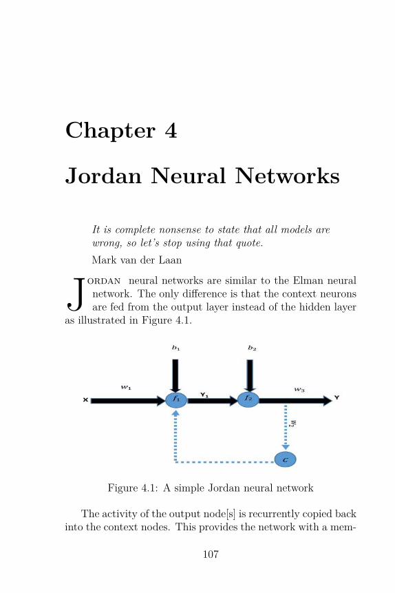
Chapter 4
Jordan Neural Networks
It is complete nonsense to state that all models arewrong, so let’s stop using that quote.Mark van der Laan
Jordan neural networks are similar to the Elman neuralnetwork. The only difference is that the context neuronsare fed from the output layer instead of the hidden layer
as illustrated in Figure 4.1.
Figure 4.1: A simple Jordan neural network
The activity of the output node[s] is recurrently copied backinto the context nodes. This provides the network with a mem-
107

Deep Learning Made Easy with R
ory of its previous state.
Three Problems Jordan Neural Net-works Can SolveJordan neural networks have found an amazing array of uses.They appear capably of modeling timeseries data and are usefulfor classification problems. Below we outline a few illustrativeexamples of real world use of this predictive analytic tool.
The Ultimate Guide for Wind Speed Fore-castingAccurate forecasts of wind speed in coastal regions are impor-tant for a wide range of industrial, transportation and socialmarine activity. For example, the prediction of wind speed isuseful in determining the expected power output from windturbines, operation of aircraft and navigation by ships, yachtsand other watercraft. Civil Engineers Anurag and Deo77 buildJordan neural networks in order to forecast daily, weekly aswell as monthly wind speeds at two coastal locations in India.
Data was obtained from the India Meteorological Depart-ment covering a period of 12 years for the coastal location ofColaba within the Greater Mumbai (Bombay) region along thewest coast of India. Three Jordan networks for daily, weeklyand monthly wind speed forecasting were developed.
All three models had a mean square error less than 10%.However, the daily forecasts were more accurate than theweekly forecasts; and the weekly forecasts were more accuratethan the monthly forecasts. The engineers also compare thenetwork predictions to auto regressive integrated moving av-erage (ARIMA) timeseries models; They observe “The neuralnetwork forecasting is also found to be more accurate than tra-ditional statistical timeseries analysis.”
108

CHAPTER 4. JORDAN NEURAL NETWORKS
How to Classify Protein-Protein interactionProtein-protein interaction refers to the biological functionscarried out by the proteins within the cell by interacting withother proteins in other cells as a result of biochemical eventsand/or electrostatic forces. Such interactions are believed tobe important in understanding disease pathogenesis and de-veloping new therapeutic approaches. A number of differentperspectives have been used to study these interactions rang-ing from biochemistry, quantum chemistry, molecular dynam-ics, signal transduction, among others78 All this informationenables the creation of large protein interaction databases.
Computer scientists Dilpreet and Singh 79 apply Jordanneural networks to classify protein-protein interactions. Thesample used in their analysis was derived from three existingdatabases80. It contained 753 positive patterns and 656 neg-ative patterns81. Using amino acid composition of proteins asinput to the Jordan network to classify the percentage of in-teracting and non-interacting proteins the researchers report aclassification accuracy of 97.25%.
Deep Learning to Woo Spanish SpeakersNeural networks have been successfully applied to the difficultproblem of speech recognition in English82. Accurate classi-fication of the numerical digits 0 through 9 in Spanish usingJordan neural networks was investigated by researcher TellezPaola83.
In a rather small study, the speech of the ten numericaldigits was recorded with voices from three women and threemen. Each person was requested to repeat each digit four times.The network was then trained to classify the digits. Using ninerandom initializations’ Tellez reports an average classificationaccuracy of 96.1%.
109

Deep Learning Made Easy with R
Essential Elements for Effective Jor-dan Models in R
I grew up in the heart of England where the weather is alwayson the move. If you want to experience all four seasons inone day, central England is the place to visit! Anyway, in
England, the weather is always a great conversation starter. Solet’s start our exploration of Jordan networks modeling Britishweather. To be specific, we will model the temperature of thecity of Nottingham located in Nottinghamshire, England. Youmay recall this area was the hunting ground of the people’sbandit Robin Hood84. Let’s get our hands dirty and build aJordan neural network right now! As with Elman networks,Jordan networks are great for modeling timeseries data.
Which are the Appropriate Packages?We will use the RSNNS package along with the quantmod pack-age. The data frame nottem, in the datasets package, con-tains monthly measurements on the average air temperatureat Nottingham Castle85, a location Robin Hood would haveknown well:> require(RSNNS)> data("nottem",package="datasets")> require(quantmod)
Let’s take a quick peek at the data held in nottem:
110

CHAPTER 4. JORDAN NEURAL NETWORKS
There do not appear to be any missing values or rouge obser-vations. So, we can continue.
We check the class of nottem using the class method:> class(nottem)[1] "ts"
It is a timeseries object of class ts. Knowing the class of yourobservations is critically important, especially if you are usingdates or your analysis mixes different types of R classes. Thiscan be a source of many hours of frustration. Fortunately,we now know nottem is of class ts; this will assist us in ouranalysis.
Figure 4.2 shows a timeseries plot of the observations innottem. The data cover the years 1920 to 1939. There doesnot appear to be any trend evident in the data, however itdoes exhibit strong seasonality. You can replicate the chart bytyping:> plot(nottem)
111

Deep Learning Made Easy with R
Figure 4.2: Average Monthly Temperatures at Nottingham1920–1939
A Damn Good Way to TransformDataFor the most part I like to standardize my attribute data priorto using a neural network model. Whilst there are no fixed rulesabout how to normalize inputs here are four popular choices foran attribute xi:
zi = xi − xmin
xmax − xmin
(4.1)
zi = xi − xσx
(4.2)
zi = xi√SSi
(4.3)
zi = xi
xmax + 1 (4.4)
112

CHAPTER 4. JORDAN NEURAL NETWORKS
SSi is the sum of squares of xi, and x and σx are the mean andstandard deviation of xi.In this case, given that we do not have any explanatory vari-ables, we will take the log transformation and then use thescale method to standardize the data:> y<-as.ts(nottem)> y<-log(y)> y<- as.ts(scale(y))
Since we are modeling data with strong seasonality charac-teristics which appear to depend on the month, we use monthlylags going back a full 12 months. This will give us 12 attributesto feed as inputs into the Jordan network. To use the Lag func-tion in quantmod we need y to be a zoo class:> y<-as.zoo(y)> x1<-Lag(y, k = 1)> x2<-Lag(y, k = 2)> x3<-Lag(y, k = 3)> x4<-Lag(y, k = 4)> x5<-Lag(y, k = 5)> x6<-Lag(y, k = 6)> x7<-Lag(y, k = 7)> x8<-Lag(y, k = 8)> x9<-Lag(y, k = 9)> x10<-Lag(y, k = 10)> x11 <-Lag(y, k = 11)> x12<-Lag(y, k = 12)
As with the Elman network, we need to remove the laggedvalues that contain NA’s (see page 101 for further details). Thefinal cleaned values are stored in the R object temp:> temp<-cbind(x1 ,x2,x3,x4,x5 ,x6 ,x7 ,x8,x9 ,
x10 ,x11 ,x12)> temp<-cbind(y,temp)> temp <- temp [ -(1:12) ,]
113

Deep Learning Made Easy with R
As a final check, let’s visually inspect all of the attributes andresponse variable. The result is shown in Figure 4.3, and wascreated using the plot method:>plot(temp)
Figure 4.3: Response and attribute variables for Jordan net-work
Notice that Series 1 is the response variable y, and Lag 1,Lag 2,...,Lag 12 are the input attributes x1, x2,...,x12.
Here is How to Select the TrainingSampleFirst we check the number of observations (should be equal to228), then we use the set.seed method to ensure reproducibil-ity:> n=nrow(temp)> n[1] 228> set.seed (465)
For the training sample 190 observations are randomly se-lected without replacement as follows:
114

CHAPTER 4. JORDAN NEURAL NETWORKS
> n_train <- 190> train <- sample (1:n,n_train , FALSE)
Use This Tip to Estimate Your Model
The model is estimated along similar lines as the Elmanneural network on page 102. The attributes are stored in the Robject inputs. The response variable is stored in the R objectoutputs. The model is then fitted using 2 hidden nodes, witha maximum of 1000 iterations and a learning rate parameterset to 0.01:> inputs <- temp [ ,2:13]> outputs <- temp[,1]
> fit <- jordan(inputs[train],outputs[train],size=2,learnFuncParams=c(0.01) ,maxit =1000)
The plot of the training error by iteration is shown inFigure 4.4. It was created using:> plotIterativeError(fit)
The error falls sharply within the first 100 or so iterations andby around 300 iterations is stable.
115

Deep Learning Made Easy with R
Figure 4.4: Training error by iteration
Finally, we can use the predict method to forecast thevalues from the test sample. We also calculate the squaredcorrelation between the test sample response and the predictedvalues:> pred<-predict(fit , inputs[-train])
> cor(outputs[-train], pred)^2[,1]
[1,] 0.9050079
The squared correlation coefficient is relatively high at 0.90. Wecan at least say our model has had some success in predictingthe weather in Nottingham - Robin Hood would be amazed!
116

NOTES
Notes77More, Anurag, and M. C. Deo. "Forecasting wind with neural net-
works." Marine structures 16.1 (2003): 35-49.78See for example:
• Herce, Henry D., et al. "Visualization and targeted disruptionof protein interactions in living cells." Nature Communications 4(2013).
• Hoppe, Philipp S., Daniel L. Coutu, and Timm Schroeder. "Single-cell technologies sharpen up mammalian stem cell research." Naturecell biology 16.10 (2014): 919-927.
• Li, Yao-Cheng, et al. "A Versatile Platform to Analyze Low-Affinityand Transient Protein-Protein Interactions in Living Cells in RealTime." Cell reports 9.5 (2014): 1946-1958.
• Qin, Weihua, et al. "DNA methylation requires a DNMT1 ubiquitininteracting motif (UIM) and histone ubiquitination." Cell Research(2015).
79Kaur, Dilpreet, and Shailendra Singh. "Protein-Protein InteractionClassification Using Jordan Recurrent Neural Network."
80Pfam, 3did and Negatome. For further details see:
• Robert D. Finn, John Tate et. al., “The Pfam protein familiesdatabase”, Nucleic Acids Research, vol. 36, pp. 281–288, 2008.
• Amelie Stein, Robert B. Russell and Patrick Aloy, “3did: interact-ing protein domains of known three-dimensional structure”, NucleicAcids Research, vol. 33, pp. 413–417, 2005.
• Pawel Smialowski, Philipp Page et. al., “The Negatome database:a reference set of non-interacting protein pairs”, Nucleic Acids Re-search, pp. 1–5, 2009.
81Positive patterns contain interacting residues in its center. Negativepatterns contain non-interacting residues in its center.
82See:
• Lippmann, Richard P. "Review of neural networks for speech recog-nition." Neural computation 1.1 (1989): 1-38.
• Arisoy, Ebru, et al. "Bidirectional recurrent neural network lan-guage models for automatic speech recognition." Acoustics, Speechand Signal Processing (ICASSP), 2015 IEEE International Confer-ence on. IEEE, 2015.
117

Deep Learning Made Easy with R
• Sak, Haşim, et al. "Fast and Accurate Recurrent Neural Net-work Acoustic Models for Speech Recognition." arXiv preprintarXiv:1507.06947 (2015).
• Hinton, Geoffrey, et al. "Deep neural networks for acoustic mod-eling in speech recognition: The shared views of four researchgroups." Signal Processing Magazine, IEEE 29.6 (2012): 82-97.
83Paola, Tellez. "Recurrent Neural Prediction Model for Digits Recog-nition."International Journal of Scientific & Engineering Research Volume2, Issue 11, November-2011.
84See Knight, Stephen. Robin Hood: a complete study of the Englishoutlaw. Blackwell Publishers, 1994.
85If you are planning to visit, before you go take a look at:
• Hutchinson, Lucy, and Julius Hutchinson. Memoirs of the Life ofColonel Hutchinson, Govenor of Nottingham Castle and Town. G.Bell and sons, 1906.
• Drage, Christopher. Nottingham Castle: a place full royal. Not-tingham Civic Society [in association with] The Thoroton Societyof Nottinghamshire, 1989.
• Hooper-Greenhill, Eilean, and Theano Moussouri. Visitors’ Inter-pretive Strategies at Nottingham Castle Museum and Art Gallery.No. 2. Research Centre for Museums and Galleries and Universityof Leicester, 2001.
118

Chapter 5
The Secret to theAutoencoder
Though this be madness, yet there is method in’t.William Shakespeare
The autoencoder (sometimes called an autoassociator)is an unsupervised three-layer feature learning feed-forward neural network network. Architecturally, as
shown in Figure 5.1, it is very similar to the multilayer percep-tron; it includes an input layer, a hidden layer and an outputlayer. The number of neurons in the input layer is equal to thenumber of neurons in the output layer. The number of hiddenneurons is less (or more) than the number of input neurons. Itis different from an MLP because the output layer has as manynodes as the input layer, and instead of training it to predictsome target value y given inputs x, an autoencoder is trainedto reconstruct its own inputs x.
The autoencoder consists of an encoder and a decoder. Themapping of the input layer to the hidden layer is called encod-ing and the mapping of the hidden layer to the output layeris called decoding. The encoder takes the vector of input at-tributes and transforms them typically through sigmoid acti-vation functions in the hidden layers into new features. The
119

Deep Learning Made Easy with R
decoder then converts these features back to the original inputattributes. So for example, in Figure 5.1, the autoencoder takesthe attributes x1, x2, x3, x4 encodes them using three hiddenunits each containing sigmoid activation functions h1, h2, h3,and then decodes them to obtain estimates x1, x2, x3, x4 of theoriginal attributes.
Figure 5.1: Basic Autoencoder
A Jedi Mind TrickAt this point you may be wondering is this some complicatedJedi mind trick? What is the point of taking our original at-tributes, transforming them into who knows what, and thenobtaining estimates of their original values? What is going onhere?
Well, yes there is a little bit of the Jedi Master in this.You see, one of the great challenges faced by data scientists,statisticians, psychologists and others involved in data analysisis the problem of dimensionality reduction.
Here is what this issue involves: Suppose you have 300 po-tential attributes that might explain your response variable.
120

CHAPTER 5. THE SECRET TO THE AUTOENCODER
In traditional statistical modeling, it would not be possible toinclude all 300 attributes in your model. What to do? En-ter dimensionality reduction techniques, the most famous beingprincipal component analysis (PCA) developed in 1901 by Uni-versity College, London, professor of mathematics Karl Pear-son.
I first came across PCA though the classic 1972 and 1973papers of the then University of Kent at Canterbury scholar I.T. Jolliffe86; the technique has been a permanent addition tomy data science toolkit ever since. Briefly, PCA is a statisticalprocedure that uses an orthogonal transformation to converta number of (possibly) correlated attributes into a (smaller)number of uncorrelated variables called principal components.The principal components are linear combinations of the orig-inal attributes. Here are the key points to be aware of:
1. The number of principal components is less than or equalto the number of original variables.
2. The first principal component accounts for the largestproportion of the variability in the data; and each suc-ceeding component accounts for as much of the remain-ing variability as possible conditional on being orthogonal(aka uncorrelated) to the preceding components.
3. The principal components are orthogonal because theyare the eigenvectors of the covariance matrix, which is ofcourse symmetric.
The Secret RevealedI’ll always remember what Jabba the Hutt said rather pointedlyto Bib Fortuna in Return of the Jedi “You weak-minded fool!He’s using an old Jedi mind trick!” The thing about a Jedimind trick was once it was revealed to you, it lost much ofits power or became totally ineffective. Perhaps you recall the
121

Deep Learning Made Easy with R
rather humorous scene in the Phantom Menace, when Qui-GonJinn, stranded on Tatooine, attempts to use a mind trick onWatto in order to encourage him to accept Republic creditsfor the purchase of a T-14 hyperdrive. Watto interjects “...youthink you’re some kind of Jedi, waving your hand around likethat? I’m a Toydarian! Mind tricks don’t work on me, onlymoney! No money, no parts, no deal!”
Let’s take another look at the autoencoder “trick”,this timewithout the hand waving! An autoencoder is a feed forwardneural network used to learn representations of data. The ideais to train a network with at least one hidden layer to recon-struct its inputs. The output values are set equal to input val-ues, i.e. x = x in order to learn the identity function h(x) ≈ x.The autoencoder achieves this by mapping input attributes tohidden layer nodes using an encoder function:
h(x) = f(Wx+ bh)
where x is the input vector of attributes, f denotes the sigmoidfunction, bh is the vector of hidden neuron biases, andW is thematrix of hidden weights. The data is reconstructed using alinear decoder:
g(x) = λf(Wx+ bh) + bg
After learning the weights W , each hidden neuron representsa certain feature of the input data. Thus, the hidden layerh(x) can be considered as a new feature representation of theinput data. The hidden representation h(x) is then used toreconstruct an approximation x of the input using the decoderfunction g(x).
The most commonly used function for the encoder anddecoder is a nonlinear sigmoid function. Training is typi-cally achieved by minimizing the squared reconstruction error(g(x) − x)2 using the backpropagation by gradient descent al-gorithm. In practice, the restriction λ = W T is often imposedto reduce the number of parameters.
122

CHAPTER 5. THE SECRET TO THE AUTOENCODER
The key thing to keep in mind is that by learning the hid-den representation h(x) that can reconstruct the original inputattributes, the autoencoder captures important features of theinput attributes. For example, if the number of hidden layerneurons is larger than the number of input layer neurons thehidden layers map the input to a higher dimension. Similarly, ifthe number of hidden neurons is less than the number of inputneurons the autoencoder’s hidden layer essentially compressesthe input attributes in such a way that they can be efficientlyreconstructed87.
The compressed representation has lower dimensionalitythan the original input attributes. For example, when an au-toencoder has 400 input neurons and 60 hidden nodes, theoriginal 400-dimensional input is ‘reconstructed’ approximatelyfrom the 60-dimensional output of the hidden layer. If we usethe output of the hidden layer as a representation of an in-put of the network, the autoencoder plays the role of a featureextractor.
It turns out that autoencoders can implement a variety ofdimensionality reduction techniques. A linear autoencoder canlearn the Eigenvectors of the data equivalent to applying PCAto the inputs88. A nonlinear autoencoder is capable of dis-covering more complex, multi-modal structure in the data. Incertain situations, a nonlinear autoencoder can even outper-form PCA for certain dimensionality reduction tasks involvedwith handwriting and face recognition89.
Autoencoders can therefore be used to learn a compressed(or expanded) representation of data with minimum recon-struction loss. As pointed out by deep learning scholar Ge-offrey Hinton90 “It has been obvious since the 1980s that back-propagation through deep autoencoders would be very effectivefor nonlinear dimensionality reduction, provided that comput-ers were fast enough, data sets were big enough, and the initialweights were close enough to a good solution. All three con-ditions are now satisfied. Unlike nonparametric methods, au-toencoders give mappings in both directions between the data
123

Deep Learning Made Easy with R
and code spaces, and they can be applied to very large data setsbecause both the pretraining and the fine-tuning scale linearlyin time and space with the number of training cases.”
A Practical Definition You Can RunWithWe can summarize by stating that an autoencoder is an artifi-cial neural network that attempts to reproduce its input, i.e.,the target output is the input. Another way of saying this, anda little more formal is that an autoencoder is a feedforwardneural network that tries to implement an identity function bysetting the outputs equal to the inputs during training. Theparameters are learned by minimizing a loss functions. Theloss function measures the difference between input attributesand output. Stochastic Gradient Descent is typically used tominimize the loss function:
L(x, x) = −k∑
i=1[xi log xi + (1− xi) log (1− xi)]
How to Save the Brazilian CerradoLet’s look at a very practical application of an autoencoder asa feature extractor. Since the environment impacts us all, wetake our example from environmental and space science.
The Brazilian Cerrado, at almost three times the size ofTexas, is the world’s most biologically rich savanna. It containsover 10,000 species of plants, of which 45% are exclusive tothe Cerrado, feeds three of the major water basins in SouthAmerica: the Amazon, Paraguay and São Francisco Rivers.
Brazilian National Institute for Space Research researchersCosta Wanderson, Leila Fonseca, and Thales Körting reportover 500,000km2 of this pristine and marvelous landscape hasbeen industrialized into cultivated pastures over the past few
124

CHAPTER 5. THE SECRET TO THE AUTOENCODER
years91. The rate of change is so rapid the researchers observewith concern that it outpaces even the stunning intensity ofcommercialization and industrialization in the Amazon region.
The consequence, for the Brazilian Cerrado, as Wander-son, Fonseca, and Körting state is that “...nearly 50% of thecultivated pasture areas are severely degraded, causing loss ofsoil fertility, increased erosion and predominance of invasivespecies.”
Moderate Resolution Imaging Spectroradiometer data fromthe Terra and Aqua satellites was collected by the researchersto perform image classification for a small region focused onthe Serra da Canastra National Park.
The researchers ended up with a total of 30 input attributes,23 of which were obtained from spectral bands. Given thenumber of attributes, the researchers required a technique toreduce the dimensionality. An Autoencoder was developed andsuccessfully used to reduce the dimensionality of the data.
Analysis was performed using a reduced set of 15 attributesand a reduced set of 25 attributes. The researchers conclude“...using a smaller number of attributes from the autoencoderhad accuracies similar to those obtained in the tests that usedall original attributes, emphasizing the ability of this network[the autoencoder] to reduce the dimensionality of the data.”
The Essential Ingredient You Need toKnowThe key ingredient in an autoencoder are the input attributes.It is important to realize that if the input attributes containno structure then compression will prove futile. For example,if the input attributes are completely random, compression isunfeasible. Effective compression requires the attributes to becorrelated or related in some way. In other words, there needsto be some structure that can be used to decompress the data.
125

Deep Learning Made Easy with R
If that structure is not present, using an autoencoder for di-mensionality reduction will likely fail.
The Powerful Benefit of the SparseAutoencoderA sparse autoencoder uses a large number of hidden neurons,where only a small fraction are active. A nonlinear mappingof the input vector x is made by setting the number of hiddenneurons92 much larger than the number of input neurons93 andthen enforcing a sparsity constraint on them. Training there-fore involves using a sparsity constraint to learn sparse repre-sentations of the data. The most popular sparsity constraintuses the Kullback-Leibler (KL) divergence.
Understanding Kullback-Leibler Di-vergenceKullback- Leibler divergence is a distance measure from a "true"probability distribution to a "target" probability distributionof a Bernoulli random variable with mean p and a Bernoullirandom variable with mean pj:
KL(p||pj) = p log(p
pj
)+ (1− p) log
(1− p1− pj
)
Note that KL(p||pj) = 0 for p = pj , otherwise it is positive.The parameter p is the sparsity parameter, which is usually
set to a small value. It is the frequency of the activation ofhidden nodes; for example, if p =0.07, the average activationof neuron j is 7%.
126

CHAPTER 5. THE SECRET TO THE AUTOENCODER
Let’s denote the activation of the hidden neuron j for inputattribute xi by let a(2)
j (xi) and define:
pj = 1n
n∑i=1
[a
(2)j (xi)
]
The parameter pj is the average threshold activation of thehidden neuron j over all training samples. In order to computepj, the entire training set needs to be propagated forward tocompute all units’ activation’s; followed by stochastic gradientdescent using backpropagation. This makes it computationallyexpensive relative to the standard autoencoder.
The sparsity optimization objective for unit j is p = pj whichis obtained by adding the following sparsity constraint whenminimizing the squared reconstruction error or loss function:
α∑
j
KL(p||pj)
where α is a hyperparmeter that determines the relative im-portance of the sparseness term in the overall autoencoder lossfunction. To see this note that in general, an autoencoder findsthe weights to minimize:
arg minW,b
J(W, b) = L(x, x)
Here L is a loss function such as the squared error or cross-entropy, W the weights and b the biases. For the sparse au-toencoder we have:
JSparse(W, b) = J(W, b) + α∑
j
KL(p||pj)
So we see that the sparsity term adds a positive value to theoverall autoencoder loss function for p 6= pj.
127

Deep Learning Made Easy with R
Three Timeless Lessons from theSparse AutoencoderLesson 1: In practice many more applications are developed
using the sparse autoencoder than the standard autoen-coder; mainly because a greater variety of models can belearned, depending on the activation function, number ofhidden units and nature of the regularization used duringtraining.
Lesson 2: Another rationale for using a sparse encoding forclassification is that features that allow for a sparse repre-sentation are more likely to encode discriminatory prop-erties of the original input data.
Lesson 3: Finally, if the hidden layer has more neurons unitsthan the input layer, the standard autoencoder can po-tentially learn the identity function and thereby not ex-tract useful features from the input attributes.
Mixing Hollywood, Biometrics andSparse AutoencodersBiometrics techniques occur frequently in Hollywood Movies.You may have noticed this. I am amazed at how frequentlythis fantastic identification technology rears its head on thebig screen. In almost every portrayal of the future, especiallyin dystopian futures, it plays an important role. Actors canbe seen peering into eye scanners that monitor the capillaryvessels located at the back of the eye or assess the colored ringthat surrounds the eye’s pupil. They can be seen waving theirhands at sensors to open doors, start up space-craft and fireweapons. From the computer that analyses voice and facialexpressions, to the sensitive door that opens when a hand is
128

CHAPTER 5. THE SECRET TO THE AUTOENCODER
placed on the identification pad, biometric techniques are allover the movies.
Scanning live eyeballs with blue lights, passing laser likebeams over hands or even digital bulbs flashing manically asa disobedient computer assesses vocal patterns and rotates itsbeady camera like eye to assess facial expressions, make foradded excitement in a movie.
Alas, it seems, finger vein authentication which is real andworks, lacks the excitement factor demanded by Hollywood. Isuspect this is due to the very limited amount of drama andvisual excitement screen playwrights can generate from an in-dividual placing their finger on a small glass plate. This israther a shame because finger vein authentication is a highlypractical, fast, non-invasive means of making sure people reallyare who they claim to be.
It is part of our present, and will likely persist as a biomet-ric technique well into the future. This may be why Iranianscholar Mohsen Fayyaz and colleagues94 created an interestingapproach to finger vein verification using a sparse autoencoder.
The SDUMLA-HMT Finger Vein database95 was used asthe source of the vein images. This dataset contains 3,816 fingervein images. It was collected as follows - each subject includedin the database provided images of his/her index finger, middlefinger and ring finger of both hands, and the collection for eachof the 6 fingers was repeated 6 times to obtain 6 finger veinimages. Vein images were captured using infrared scanner, seeFigure 5.2.
Fayyaz et al. apply PCA to reduce the size of input dataattributes and a sparse autoencoder with 4000 neurons in thehidden layer and the Kullback- Leibler sparsity constraint. Theautoencoder was trained on 3,000 images which excluded im-ages of individual’s right hand index finger. These were usedfor the test sample, a total of 600 images.
129
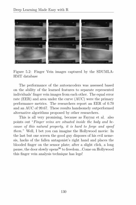
Deep Learning Made Easy with R
Figure 5.2: Finger Vein images captured by the SDUMLA-HMT database
The performance of the autoencoders was assessed basedon the ability of the learned features to separate representedindividuals’ finger vein images from each other. The equal errorrate (EER) and area under the curve (AUC) were the primaryperformance metrics. The researchers report an EER of 0.70and an AUC of 99.67. These results handsomely outperformedalternative algorithms proposed by other researchers.
This is all very promising, because as Fayyaz et al. alsopoints out “Finger veins are situated inside the body and be-cause of this natural property, it is hard to forge and spoofthem.” Well, I bet you can imagine the Hollywood movie: Inthe last but one screen the good guy disposes of his evil neme-sis, hacks of the fallen antagonist’s right hand and places theblooded finger on the sensor plate; after a slight click, a longpause, the door slowly opens96 to freedom...Come on Hollywoodthis finger vein analysis technique has legs!
130

CHAPTER 5. THE SECRET TO THE AUTOENCODER
How to Immediately use the Autoen-coder in REnough talking now let’s get to work with R! The R logo shouldbe pretty familiar to you. Let’s put some of the ideas we havediscussed into action and build a sparse autoencoder to com-press the R logo image and extract hidden features. First, loadthe required packages:> require(autoencoder)> require(ripa)
The package autoencoder contains the functions we need tobuild a sparse autoencoder. The ripa package contains animage of the R logo. The image is loaded into R as follows:> data(logo)
Go ahead, take a look at logo, you will see the image shownin Figure 5.3:> image(logo)
Let’s take a look at the characteristics of logo:> logosize: 77 x 101type: grey
It is a grey scale image of size 77 by 101 pixels.Next, make of copy of the image and store in x_train. The
image is transposed with t() to make it suitable for use withthe package autoencoder.> x_train <-t(logo)
> x_trainsize: 101 x 77type: grey
So, we see x_train is a grey scale image with 101 rows (cases)and 77 columns (attributes).
131

Deep Learning Made Easy with R
Figure 5.3: The R logo using image
Now we are ready to specify a sparse autoencoder using theautoencode function. Here is how to do that:> set.seed (2016)
> fit<-autoencode(X.train=x_train ,+ X.test = NULL ,+ nl = 3,+ N.hidden = 60,+ unit.type = "logistic",+ lambda = 1e-5,+ beta = 1e-5,
132

CHAPTER 5. THE SECRET TO THE AUTOENCODER
+ rho = 0.3,+ epsilon =0.1,+ max.iterations = 100,+ optim.method = c("BFGS"),+ rel.tol =0.01 ,+ rescale.flag = TRUE ,+ rescaling.offset = 0.001)
The first line of autoencode indicates the model will be storedin the R object fit; it also passes the image data in x_trainto the function. The parameter nl refers to the number oflayers and is set to 3. The number of hidden nodes equals 60with logistic activation functions. The parameter lambda is aweight decay parameter, typically set to a small value; the sameholds true of beta, which is the weight of the sparsity penaltyterm. The sparsity is set to 0.3 (rho) and sampled from anormal distribution N(0,epsilon2). The maximum number ofiterations is set to 100. Notice that rescale.flag = TRUE touniformly rescale the training matrix x_train so its values liein the range 0-1 (for the logistic activation function).
The attributes associated with fit can be viewed as follows:> attributes(fit)$names[1] "W" "b"[3] "unit.type" "rescaling"[5] "nl" "sl"[7] "N.input" "N.hidden"[9] "mean.error.training.set" "mean.error.
test.set"
$class[1] "autoencoder"
Let’s take a look at the "mean.error.test.set":> fit$mean.error.training.set[1] 0.3489713
133

Deep Learning Made Easy with R
As we have seen previously, it is often useful to extract thefeatures of the hidden nodes. This is easily achieved using thepredict function with hidden.output=TRUE:> features <- predict(fit , X.input=x_train ,
hidden.output=TRUE)
Since the number of hidden nodes is set to 60 and the numberof attributes (columns) is 77, the features are a compact repre-sentation of the original image. A visual representation of thefeatures is shown in Figure 5.4 and can be obtained using:> image(t(features$X.output))
The transpose function t() is used to re-orientate the featuresto match Figure 5.3.
NOTE... �
The autoencode function uses the Nelder–Mead,quasi-Newton and conjugate-gradient algorithmsby calling the optim function contained in thestats package97. Available optimisation methodsinclude:
• "BFGS" is a quasi-Newton method, it usesfunction values and gradients to build up apicture of the surface to be optimized.
• "CG" is a conjugate gradients method whichis generally more fragile than the BFGSmethod. Its primary advantage is withlarge optimization problems because it workswithout having to store large matrices.
• "L-BFGS-B" allows each variable to be givena lower and/or upper bound.
134

CHAPTER 5. THE SECRET TO THE AUTOENCODER
Figure 5.4: Hidden node features extracted from fit
How well do these compressed features capture the originalimage? To reconstruct values use the predict function withhidden.output =FALSE:
> pred<- predict(fit , X.input=x_train ,hidden.output=FALSE)
The mean square error appears reasonably small:> pred$mean.error[1] 0.3503714
Let’s take a look at the reconstructed image:
135
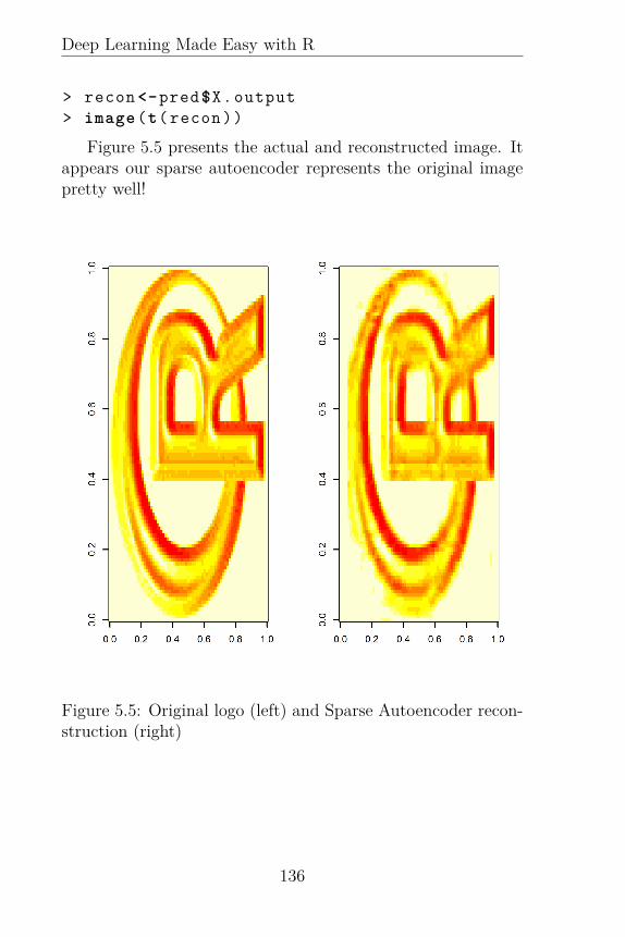
Deep Learning Made Easy with R
> recon <-pred$X.output> image(t(recon))
Figure 5.5 presents the actual and reconstructed image. Itappears our sparse autoencoder represents the original imagepretty well!
Figure 5.5: Original logo (left) and Sparse Autoencoder recon-struction (right)
136

CHAPTER 5. THE SECRET TO THE AUTOENCODER
An Idea for Your Own Data ScienceProjects with RIn this section we perform an analysis of an edible mollusk usingthe autoencoder and R. As you work through this section, thinkabout how you might adapt the approach for you own research.
Abalone are, mostly sedentary, marine snails and belong toa group of sea critters (phylum Mollusca) which include clams,scallops, sea slugs, octopuses and squid. They cling to rockswhile waiting for their favorite food of kelp to drift by. Oncethe seaweed is spotted they hold it down, with what can onlybe described as a “foot”, and chew on it vigorously (for a snail)with radula - a rough tongue with many small teeth.
Given the healthy diet of fresh kelp it is little wonder thesemollusks are considered delicious raw or cooked. They aredeemed to be so flavorful that the demand for consumption out-stripped supply over many years. Today, the white abalone isofficially listed as an endangered species. Other species remainplentiful, are harvested regularly to the delight of foodies98,restaurant goers and seafood chefs99.
The abalone dataset from UCI Machine Learning Archiveswas collected to predict abalone age (through the number ofrings on the shell) given various attributes such as shell sizes(height, length, width), and weights (shell weight, shuckedweight, viscera weight, whole weight). Here is how to capturethe web link to the dataset100 using R:> aburl = ’http://archive.ics.uci.edu/ml/
machine -learning -databases/abalone/abalone.data’
The observations are loaded into R using read.table andstored in the R object data:> names = c(’sex’,’length ’,’diameter ’,’height ’,
137

Deep Learning Made Easy with R
’whole.weight ’,’shucked.weight ’,’viscera.weight ’,’shell.weight ’,’rings’)
> data = read.table(aburl ,header = F ,sep = ’,’,col.names = names)
To investigate the data for unusual observations I often usethe summary function. The annotated result is shown below:>summary(data)
We can tell instantly there exists a problem with the abaloneheight; some of the snails are recorded as having 0 height. Thisis not possible! We will need to investigate further. To take alook at those values enter:> data[data$height ==0,]
138

CHAPTER 5. THE SECRET TO THE AUTOENCODER
It appears two observations have been erroneously recordedwith zero height (observation 1258 and observation 3997). Weneed to re-code these observations as missing and remove themfrom sample.> data$height[data$height ==0] = NA> data <-na.omit(data)
Next, we drop the sex variable from the sample.> data$sex<-NULL
We take another look at the data using summary:>summary(data)
All seems reasonable.Next, we transpose the data, convert it to a matrix and
store the result in the R object data1:> data1 <-t(data)> data1 <-as.matrix(data1)
Now we load the autoencoder package, sample 10 observa-tions without replacement and create the basic model which isstored in the R object fit:require(autoencoder)
> set.seed (2016)
139

Deep Learning Made Easy with R
> n=nrow(data)> train <- sample (1:n, 10, FALSE)
> fit<-autoencode(X.train=data1[,train],+ X.test = NULL ,+ nl = 3,+ N.hidden = 5,+ unit.type = "logistic",+ lambda = 1e-5,+ beta = 1e-5,+ rho = 0.07,+ epsilon =0.1,+ max.iterations = 100,+ optim.method = c("BFGS"),+ rel.tol=0.01 ,+ rescale.flag = TRUE ,+ rescaling.offset = 0.001)
Much of this we have seen before; the key thing to note is thatwe fit a model with 5 hidden nodes and a sparsity parameterof 7%.
Once the model is optimized, you should observe a meansquare error less than 2%:> fit$mean.error.training.set[1] 0.01654644
The features can be observed, as we saw earlier, by settinghidden.output=TRUE. Since the number of hidden nodes is lessthan the number of features the output of features$X.outputcaptures a compressed representation of the data:> features <- predict(fit , X.input=data1[,
train], hidden.output=TRUE)> features$X.output
140

CHAPTER 5. THE SECRET TO THE AUTOENCODER
Let’s use the predict function to reconstruct the valuesand store the result in the R object pred:> pred<- predict(fit , X.input=data1[,train
], hidden.output=FALSE)
Figure 5.6, Figure 5.7 and Figure 5.8 use a radar plot tovisualize the reconstructed values.
Overall the reconstructed values offer a reasonable repre-sentation of the original values. However, notice the apparentpoor fit of observation 5 and to a lesser extent observation 6;let’s investigate a little further.
The barplot of Figure 5.9 shows the difference between thereconstructed values and observed values. It appears the re-constructed observations under-fit on all eight dimensions (at-tributes). This is most apparent in observation 5 with ringswhere the reconstructed rings attribute has a value of 1.4 ver-sus the observed value of 3.5. A similar pattern is observedwith observation 6.
141

Deep Learning Made Easy with R
Figure 5.6: Observed and reconstructed values for observations1 to 4
142

CHAPTER 5. THE SECRET TO THE AUTOENCODER
Figure 5.7: Observed and reconstructed values for observations5 to 8
143

Deep Learning Made Easy with R
Figure 5.8: Observed and reconstructed values for observations9 and 10
Figure 5.9: Barplot of differences
144

NOTES
Notes86I strongly recommend you get a copy and read thoroughly both of the
following papers. They are pure solid gold:
• Jolliffe, Ian T. "Discarding variables in a principal component anal-ysis. I: Artificial data." Applied statistics (1972): 160-173.
• Jolliffe, Ian T. "Discarding variables in a principal component anal-ysis. II: Real data." Applied statistics (1973): 21-31.
87See:
• Bengio, Yoshua. "Learning deep architectures for AI." Foundationsand trends® in Machine Learning 2.1 (2009): 1-127.
• Deng, Li, et al. "Binary coding of speech spectrograms using a deepauto-encoder." Interspeech. 2010.
88See Rostislav Goroshin and Yann LeCun. Saturating Auto-Encoders.International Conference on Learning Representations, 2013.
89See Hinton, Geoffrey E., and Ruslan R. Salakhutdinov. "Reducingthe dimensionality of data with neural networks." Science 313.5786 (2006):504-507.
90Hinton, Geoffrey E., and Ruslan R. Salakhutdinov. "Reducing thedimensionality of data with neural networks." Science 313.5786 (2006):504-507.
91Costa, Wanderson, Leila Fonseca, and Thales Körting. "ClassifyingGrasslands and Cultivated Pastures in the Brazilian Cerrado Using Sup-port Vector Machines, Multilayer Perceptrons and Autoencoders." Ma-chine Learning and Data Mining in Pattern Recognition. Springer Inter-national Publishing, 2015. 187-198.
92The layer of the hidden units is often referred to as the bottleneck.93The situation where the number of hidden neurons is larger than the
number of input neurons is often referred to as “overcomplete”.94Fayyaz, Mohsen, et al. "A Novel Approach For Finger Vein Verifi-
cation Based on Self-Taught Learning." arXiv preprint arXiv:1508.03710(2015).
95Developed by Shandong University and available at http://mla.sdu.edu.cn/sdumla-hmt.html
96Yes, I am aware that technically this won’t actually work. As Fayyazmakes clear “Another key property of finger vein pattern authenticationis the assurance of aliveness of the person, whose biometrics are be-ing proved.” Hey, but we are talking Hollywood where creative licenseabounds!
145

Deep Learning Made Easy with R
97R Core Team (2015). R: A language and environment for statisticalcomputing. R Foundation for Statistical Computing, Vienna, Austria.URL https://www.R-project.org/.
98For the foodies among you here are a few East Coast (USA) restau-rants which serve abalone steaks:
• Allegretto Vineyard Resort Paso Robles 805-369-2500http://www.ayreshotels.com/allegretto-resort-and-vineyard-paso-robles
• Artisan Paso Robles 805-237-8084 http://artisanpasorobles.com
• Windows on the Water Morro Bay 805-772-0677http://www.windowsmb.com
• Madeline’s Cambria 805-927-4175http://www.madelinescambria.com
• The Black Cat Cambria 805-927-1600http://www.blackcatbistro.com
• Linn’s Restaurant Cambria 805-927-0371http://www.linnsfruitbin.com/Linns_Restaurant.html
• Madonna Inn San Luis Obispo 805-543-3099See for example Chef Rick Moonen who states "We believe in the im-
portance of buying and serving seafood that comes from abundant popula-tions which are under sound management. All fish on our menu are caughtor farmed in a way that is not harmful to the ocean environment or toother ocean creatures. We are strong supporters of local fishing communi-ties and take responsibility for our role in preserving a lasting and diversesupply of seafood." For more information on great sustainable seafood visithttp://rickmoonen.com/
100For additional details please see http://archive.ics.uci.edu/ml/machine-learning-databases/abalone/abalone.names
146

Chapter 6
The Stacked Autoencoderin a Nutshell
The stacked autoencoder (SA) is a deep network withmultiple layers. Each layer is an autoencoder in whichthe outputs of each layer are wired to the inputs of
the successive layers. The number of units in the intermediatelayers tends to get progressively smaller in order to produce acompact representation.
Figure 6.1 illustrates a stacked autoencoder with two hid-den layers for binary classification from the research paper ofJirayucharoensak, Pan-Ngum, and Israsena101. In this exam-ple, four attributes {x1,x2,x3,x4} are fed into the stacked au-toencoder. The nodes with +1 at their center represent thebias. The attribute data is passed through two hidden lay-ers, each containing three nodes. The output layer consists ofa softmax activation function which calculates the probabilitythat the output belongs to a specific class (in this case class 0or class 1). Notice that for classification the softmax layer willusually have one output node per class.
147

Deep Learning Made Easy with R
Figure 6.1: Stacked autoencoder with two hidden layers for bi-nary classification. Image source Jirayucharoensak et al. citedin endnote sec. 101.
The Deep Learning Guru’s SecretSauce for TrainingA few years ago a rather surprising observation emerged fromthe machine learning research community. It appeared, tomany people’s surprise, that neural networks with multiplelayers were easily trainable, provided one followed a specifictechnique102. These ’deep’ neural networks, the subject ofthis book, actually outperformed single layer models in spe-cific tasks. What was the training process that led to the out-performance and shocked the machine learning community?
In essence the training of a SA or other deep networks forclassification tasks proceeds one layer at a time through anunsupervised pre-training phase.
Here is how it works. The first hidden layer is trained on the
148

CHAPTER 6. THE STACKED AUTOENCODER IN . . .
input attributes. During this process the weights and bias pa-rameters are optimized using a loss function such as the squarederror or cross-entropy.
Next, the algorithm propagates the input attributesthrough the trained first hidden layer to obtain the primaryfeatures. These features are then used to train the next hid-den layer. Once trained, the primary features are propagatedforward through the trained second layer resulting in a set ofsecondary features. These features are used as input to trainthe third layer. Each subsequent layer performs a similar pro-cedure. The last hidden layer passes its trained features tothe output layer which, typically using a softmax activationfunction, calculates the probability of each class.
Finally, the model is fine-tuned by using backpropagationacross the entire network to learn weights and biases given la-beled training examples. The objective being to minimize thenetwork error, often in terms of the confusion matrix or cross-entropy.
Whilst the above procedure represents the traditional ap-proach to training a SA some researchers have raised doubtson the necessity of the pre-training step103. Since data scienceis a series of failures punctuated by the occasional success, thebest advice nearly always, is to experiment.
How Much Sleep Do You Need?How much sleep do you enjoy each night? How much wouldyou like? Are you getting the recommended amount?Sleep scholars Webb and Agnew suggest 9 to 10 hours per nightfor optimal benefit104. Are you getting that much?Don’t worry if you are not consistently hitting 10 hours. Yousee, sleep researcher Jim Horne105, in his comprehensive trea-tise, argues between 4.5 to 6 hours per night maximum. Appar-ently, according to Jim, you can easily adapt to a 5 or 6 hoursleep schedule; anything more than this is “optional”, mere
149

Deep Learning Made Easy with R
restful “gravy”, unnecessary to fulfill your physical need forsleep or prevent the accumulation of that hazy feeling whichis the result of sleep deficit. It seems experts in the field, whohave studied the phenomenon for years have wildly differentsuggestions.
The lack of a clear scientific answer has not stopped the pop-ular media from joining the sleep bandwagon. In typical mediahype, the issue is no longer about feeling a little tired (or not)when stumbling out of bed in the morning, afternoon or evening(depending on your lifestyle); instead is has somehow mutatedinto a desperate battle between life and death. The heavy-weight Time Magazine reported106 “Studies show that peoplewho sleep between 6.5 hr. and 7.5 hr. a night...live the longest.And people who sleep 8 hr. or more, or less than 6.5 hr., theydon’t live quite as long.” Shawn Youngstedt, a professor inthe College of Nursing and Health Innovation at Arizona StateUniversity Phoenix is reported in the Wall Street Journal107as noting “The lowest mortality and morbidity is with sevenhours.” In the same article Dr. Youngstedt, a scholar in theeffects of oversleeping, warns “Eight hours or more has consis-tently been shown to be hazardous.” All this adds new meaningto the phrase “Snooze you lose”. It seems that extra lie in onSunday mornings might be killing you.
Not to worry, another, perhaps more sober headed, panelof respected sleep scholars has suggested108 “7 to 9 hours foryoung adults and adults, and 7 to 8 hours of sleep for olderadults.” Whatever is the precise number of hours you get eachnight or actually need, I think we can all agree that a restfulnight of calm relaxing sleep can work wonders after a hectic,jam packed day.
According to the American Academy of Sleep Medicine109restful sleep is a process which passes through five primarystages. These are rapid eye movement, stages N1, N2, slowwave sleep (N3) and waking up (W). Each specific stage can bescientifically measured by electrical brain activity recorded us-ing a polysomnogram with accompanying hypnograms (expert
150

CHAPTER 6. THE STACKED AUTOENCODER IN . . .
annotations of sleep stages) used to identify the sleep stage.This process, as you might expect is manually intensive andsubject to human error.
Imperial College, London scholars Orestis Tsinalis, PaulMatthews and Yike Guo develop a SA to automatically scorewhich stage of sleep an individual is in110. The present ap-proach to scoring sleep phases is inefficient and prone to error.As Tsinalis, Matthews and Guo explain “...one or more expertsclassify each epoch into one of the five stages (N1, N2, N3, R orW) by quantitatively and qualitatively examining the signals ofthe PSG [polysomnogram] in the time and frequency domains.”
The researchers use an open sleep dataset111. The sleepstages were scored by individual experts for 20 healthy sub-jects, 10 male and 10 female, aged 25–34 years. With a totalof around 20 hours of recordings per subject. Because of animbalance between the response classes (sleep stages) the re-searchers use a class-balanced random sampling scheme withan ensemble of autoencoder classifiers, each one being trainedon a different sample of the data.
The final model consisted of an ensemble of 20 independentSA all with the same hyperparameters. A type of majorityvoting was used to determine the classification of epochs; theresearchers took the mean of the class probabilities from theindividual SA’s outputs, selecting the class with the highestprobability.
The confusion matrix is shown in Figure 6.2. For all sleepstages the classification was correct at least 60% of the time.The most accurate classification of sleep stage occurred for N3(89%), followed by W (81%). Notice the upper and lower tri-angle of the confusion matrix are similar to what you mightobserve in a correlation matrix being almost mirror images ofeach other. This is an indication that the misclassification er-rors due to class imbalances have been successfully mitigated.
The researchers also compare their approach to other meth-ods developed in the literature. On every performance metricconsidered their approach outperforms by a wide margin.
151

Deep Learning Made Easy with R
The clear superiority of their results encourages Tsinalis,Matthews and Guo to confidently proclaim “To the best of ourknowledge our method has the best performance in the literaturewhen classification is done across all five sleep stages simulta-neously using a single channel of EEG [Electroencephalogra-phy].”
Figure 6.2: Confusion matrix of Tsinalis, Matthews and Guo.The numbers in bold are numbers of epochs. The numbers inparentheses are the percentage of epochs that belong to the classclassified by the expert (rows) that were classified by their algo-rithm as belonging to the class indicated by the columns. Sourceof table: Tsinalis, Matthews and Guo cited in endnote numbersec. 110.
Tsinalis, Matthews and Guo have unleashed the power ofSA to make major improvements in their field of interest. Whowould disagree with the development of automatic classifica-tion machines for sleep stage? The deployment and widespreadadoption of such machines could be an important step forwardfor researchers in the entire field of sleep studies. Who knows,maybe it will help to settle the question of “How much sleepdo you need?”
152

CHAPTER 6. THE STACKED AUTOENCODER IN . . .
Build a Stacked Autoencoder in LessThan 5 MinutesLet’s continue with the abalone data used on page 137. Weshould be able to build a stacked autoencoder pretty quickly.The model can be estimated using the SAENET.train functionfrom the package SAENET. First we load the data following ex-actly the same steps as we did on page 137. First, load thepackages and download the data from the internet:> require(SAENET)> aburl = ’http://archive.ics.uci.edu/ml/
machine -learning -databases/abalone/abalone.data’
> names = c(’sex’,’length ’,’diameter ’,’height ’,’whole.weight ’,’shucked.weight ’,’viscera.weight ’,’shell.weight ’,’rings’)
> data = read.table(aburl , header = F , sep= ’,’, col.names = names)
Next, drop the gender attribute, delete the observations withmiscoded height, and store the resultant sample as a matrix inthe R object data1:> data$sex<-NULL> data$height[data$height ==0] = NA> data <-na.omit(data)> data1 <-as.matrix(data)
Now onto the sample. Again, for illustration we will only sam-ple 10 observations:> set.seed (2016)> n=nrow(data)> train <- sample (1:n, 10, FALSE)
Now we are ready to estimate the model. In this case we fita model with 3 hidden layers with 5, 4 and 2 nodes respectively{n.nodes = c(5,4,2)}. The remainder of the following code
153

Deep Learning Made Easy with R
is familiar to you by now. The model is stored in the R objectfit:
> fit<-SAENET.train(X.train=data1[train ,],+ n.nodes = c(5,4,2),+ unit.type = "logistic",+ lambda = 1e-5,+ beta = 1e-5,+ rho = 0.07,+ epsilon =0.1,+ max.iterations = 100,+ optim.method = c("BFGS"),+ rel.tol=0.01 ,+ rescale.flag = TRUE ,+ rescaling.offset = 0.001)
The output from each layer can be viewed by typingfit[[n]]$X.output where n is the layer of interest. For ex-ample, to see the output from the two nodes in the third layer:> fit [[3]]$X.output
[,1] [,2]753 0.4837342 0.4885643597 0.4837314 0.48856843514 0.4837309 0.4885684558 0.4837333 0.48856531993 0.4837282 0.4885726506 0.4837351 0.48856212572 0.4837315 0.48856843713 0.4837321 0.488567411 0.4837346 0.4885632223 0.4837310 0.4885684
Figure 6.3 plots the outputs by observation, where for clar-ity item 753 is labeled as observation 1, item 597 is labeled asobservation 2, ..., and item 223 is labeled as item 10.
154
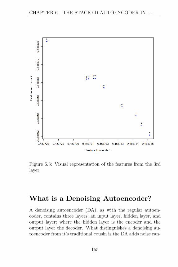
CHAPTER 6. THE STACKED AUTOENCODER IN . . .
Figure 6.3: Visual representation of the features from the 3rdlayer
What is a Denoising Autoencoder?A denoising autoencoder (DA), as with the regular autoen-coder, contains three layers; an input layer, hidden layer, andoutput layer; where the hidden layer is the encoder and theoutput layer the decoder. What distinguishes a denoising au-toencoder from it’s traditional cousin is the DA adds noise ran-
155

Deep Learning Made Easy with R
domly to the input during training. It is a stochastic variant ofautoencoder. The addition of noise prevents the hidden layerfrom simply learning the identity function and forces it to un-cover more robust features.
The Salt and Pepper of RandomMaskingGiven the input attribute vector x, the DA produces a new“noisy” attribute vector x. Whilst there are many ways to in-troduce noise, one of the most frequently used is random mask-ing. In random masking inputs are randomly set equal to zero.Notice this idea is akin to dropout where a random number ofneurons are ignored during each training round. As we saw onpage 51 dropout can significantly improve performance.
A variant, often referred to as the addition of salt and pep-per noise, randomly forces a fraction of x to be 0 or 1. Anotherpopular method involves the addition of Gaussian noise to theattribute vector x. Whichever method of noise is used the DAis then trained to reconstruct the input attributes from thenoisy version.
The Two Essential Tasks of a Denois-ing AutoencoderIntuitively the DA attempts two things:
1. First, encode the input attribute vector x;
2. second, remove the effect of the error contained in thenoisy attribute vector x.
These tasks can only be successfully achieved if the DA cap-tures the statistical dependencies between the input attributes.In practice, a DA often achieves a much better representationof the input attributes than the standard autoencoder112.
156

CHAPTER 6. THE STACKED AUTOENCODER IN . . .
How to Understand Stacked Denois-ing AutoencodersDenoising autoencoders can be stacked to form a deep learningnetwork. Figure 6.4 shows a stacked denoising autoencoder(SDA) with four hidden layers.
Figure 6.4: Stacked Denoising Autoencoder with four hiddenlayers
In a stacked denoising autoencoder (SDA) pre-training isdone one layer at a time in the same way as discussed for astacked autoencoder (see page 148). Over time it has becomeclear that pre-training often encourages the network to discovera better parameter space during the back-propagation phase.
In the pre-training phase each layer is trained as a denois-ing autoencoder by minimizing the reconstruction error. Foreach layer, feature extraction is carried out with the extractedhidden representation treated as the input to the next hiddenlayer. After the final pre-training process, the last hidden layeris classified typically with a softmax activation function andthe resulting vector passed to the output layer.
157

Deep Learning Made Easy with R
Once all layers are pre-trained, the network goes througha second stage of training, often referred to as fine tuning, viasupervised learning. At this stage the prediction error is mini-mized by backpropagation using the entire network as we wouldtrain a multilayer perceptron.
Stacking denoising autoencoders appears to improve a net-works representation ability. The more layers that are added,the more abstract are the features extracted113.
A Stunningly Practical ApplicationImaging spectroscopy has been used in the laboratory by physi-cists and chemists for well over 100 years to identify materialsand their composition. It’s popularity in the laboratory comesfrom its ability to detect individual absorption features due tospecific chemical bonds in a solid, liquid, or gas. Hyperspec-tral remote sensing takes what was once only possible in thedarkened recesses of a few scientist’s laboratory and applies itto the entire Earth.
Hyperspectral images are spectrally over-determined pro-viding sufficient spectral information to identify and distinguishbetween spectrally similar but distinct materials. Hyperspec-tral sensors typically measure reflected radiation as a series ofnarrow and contiguous wavelength bands.
It is a technology with amazing potentially to providegreatly improved discriminant capability for the detection andidentification of minerals, terrestrial vegetation, land cover clas-sification, and in fact identification of any of a stunning array ofman-made or nature produced materials. With advancing tech-nology, imaging spectroscopy has increasingly been focused onanalyzing the Earth’s surface.
As you might hazard a guess, geologists were quick to latchonto this technology for the identification and mapping of po-tential mineral deposits. They soon discovered that the actualdetection of economically exploitable minerals is dependent on
158

CHAPTER 6. THE STACKED AUTOENCODER IN . . .
a complex combination of factors including:
• The range of the spectral coverage;
• available spectral resolution,
• signal-to-noise ratio of the spectrometer,
• the actual abundance of the mineral sought;
• and the strength of absorption features for that materialin the wavelength region measured.
It is difficult to think of an area in industry, commerce or gov-ernment where this technology could not be of tremendous ben-efit.
Deep learning techniques have a role to play in this boomingand amazingly lucrative area. Think for a moment, how couldyou use deep learning to help out here?
Take a look at Figure 6.5, the answer should become im-mediately obvious to you. It shows a hyperspectral data cubefrom the innovative research of Möckel et al.114. These inno-vative scholars use hyperspectral data to discriminate betweengrazed vegetation belonging to different grassland successionalstages. Now here is the thing, Möckel et al are essentially inter-ested in a classification task. Guess what? SDA was designedfor this very purpose.
159

Deep Learning Made Easy with R
Figure 6.5: Hyperspectral data cube showing examples of dataassociated with (A) young; (B) intermediate-aged; and (C) oldgrassland sites within a subarea of 0.71 km2 within the Jordtorpstudy area. The color-composite on the top was obtained usingthree hyperspectral wavebands (RGB = 861 nm, 651 nm, and549 nm). Image source: Möckel, Thomas, et al. as cited inendnote sec. 114.
An Innovative IdeaThe potential for useful deployment of SDA for the classifi-cation of hyperspectral data is truly outstanding; a fact notmissed by the trio Chen, Li, and Xiaoquan, scholars at ChinaUniversity of Geosciences and Huazhong University of Scienceand Technology115. This trio of researchers unleash the powerof SDA for feature extraction and classification of hyperspectraldata. Their study, small and experimental, uses three imagescreated from hyperspectral data. The first image was taken
160

CHAPTER 6. THE STACKED AUTOENCODER IN . . .
over Indian Pine (INP); the second over the Okavango Delta,Botswana (BOT); and the third over the University of Pavia(PU), Italy.
Figure 6.6 shows the RGB images and the ground refer-enced information with class legends for each of the images.Table 4 shows the class information of the three image datasets,the number of classes in each image and the number of labeledsamples in each class.
Figure 6.6: Three band false color composite and ground clas-sification references. Source of image Chen Xing, Li Ma, andXiaoquan Yang as cited in endnote sec. 115.
161

Deep Learning Made Easy with R
Table 4: Class information for each image taken from the re-search paper of Chen, Li , and Xiaoquan.Source of table ChenXing, Li Ma, and Xiaoquan Yang as cited in endnote sec. 115.
Let’s take a deep dive into some of the details of the model.The first thing to observe is that the model consists of an SDAfor feature extraction and logistic regression with sigmoid acti-vation functions (LR) for fine-tuning and classification. There-fore the model, as shown in Figure 6.7, consists of a an unsu-pervised element (the SDA) and a supervised element (LR).
The second thing to observe is the parameters used in themodel are image specific. Three images equal three sets ofmodel parameters; this is akin to the parameters in a simplelinear regression being determined by the data. The slope andintercept terms can be expected to be different for distinctlydifferent datasets. In a similar way, different images may re-quire different parameter settings and therefore Chen, Li, andXiaoquan calibrated their SDA to each specific image.
The number of hidden layers was 4, 3, and 3 for BOT, PU,and INP, respectively. The number of nodes was selected as100, 300, and 200, for BOT, PU, and INP respectively. Thestandard deviation of Gaussian noise was also image specific;the researchers selected values of 0.6 for BOT/ PU, and 0.2for INP. In addition, the number of epochs used during pre-training was set to 200 for all images; with the number of finetuning epochs equal to 1500 for all images. The learning rates
162

CHAPTER 6. THE STACKED AUTOENCODER IN . . .
of pretraining and fine tuning were selected as 0.01 and 0.1respectively.
Figure 6.7: Architecture of Chen, Li , and Xiaoquan’s deeplearning model. Source of image Chen Xing, Li Ma, and Xiao-quan Yang as cited in endnote sec. 115.
How Chen, Li, and Xiaoquan Train theirModelThree steps are followed by the researchers in order to traintheir model.
• Step 1: Initial network weights are obtained by the SDAencoding component of the model.
• Step 2: The initial weights of the LR layer are set ran-domly.
163

Deep Learning Made Easy with R
• Step 3: Training data are used as input data, and theirpredicted classification results are produced with the ini-tial weights of the whole network.
• Step 4: Network weights are iteratively tuned usingbackpropagation.
How to Avoid the Sirens SongFigure 6.8 presents the images reconstructed from the optimalmodels. I think you will agree on causal observation they ap-pear to be a pretty good representation of the actual classifi-cations. This is a great start. However, as statistician GeorgeBox warned “Statisticians, like artists, have the bad habit offalling in love with their models.” Falling in love with a modelis very dangerous. The data scientist must exhibit the quali-ties of Odysseus in Homer’s Odyssey, no matter how beautifula model is to you. do not be seduced by the Sirens song. Al-ways remember that in data science there are numerous waysto achieve the same end result.
It is always a good idea to benchmark a model against com-peting alternatives, even experimental or toy models. This is animportant step towards objective professionalism. It will keepyou safe from deep potholes, especially those strewn along therocky road of model deployment for real life use.
Chen, Li, and Xiaoquan compare the classification abilityof their model (CLX) to support vector machines with linear(LSVM) and Radial basis function (RSVM) kernels. Table 5presents the results in terms of classification accuracy for allthree models. The key thing to notice is that CLX outper-formed both support vector machine for images PU and IMP.However, it under-performed RSVM for BOT.
164

CHAPTER 6. THE STACKED AUTOENCODER IN . . .
Figure 6.8: Classification results of model developed by Chen,Li , and Xiaoquan. Source Chen, Li , and Xiaoquan. Sourceof image Chen Xing, Li Ma, and Xiaoquan Yang as cited inendnote sec. 115.
Table 5: Performance results of LSVM, RSVM and CLX.Adapted from Chen, Li, and Xiaoquan. Source of table ChenXing, Li Ma, and Xiaoquan Yang as cited in endnote sec. 115.
A Challenge to You from the AuthorWhat are we to make of this? Well, have I ever told you thatData Science is a series of failures punctuated by the occasional
165

Deep Learning Made Easy with R
success? Chen, Li, and Xiaoquan have two successes and itall looks rather promising. Like Alexander Graham Bell, thepioneer of the telephone, speaking into his electronic apparatus"Watson, come here! I want to see you!"; and then hearinghis voice miraculously transmitted through wires over a short-range receiver.
NOTE... �
Alexander Graham Bell was first and foremostan astute businessman, it was not long before apatent for an "apparatus for transmitting vocal orother sounds telegraphically" was filed with theU.S. patent office116. It begins “Be it known that I,ALEXANDER GRAHAM BELL,of Salem, Mas-sachusetts, have invented certain new and usefulImprovements in Telegraphy.”
Chen, Li, and Xiaoquan’s project was experimental but sostunningly successful that further refinement and commercialapplications are sure to follow. Other astute individuals willharness the power of the SDA to develop useful systems andfollow Mr. Bell into the history books. Will one of them beyou?
The Fast Path to a Denoising Autoen-coder in RResearchers Huq and Cleland117, as part of a regular survey onthe fertility of women in Bangladesh, collected data on mobil-ity of social freedom. The sub-sample measured the responseof 8445 rural women to questions about whether they couldengage in certain activities alone (see Table 6).
166

CHAPTER 6. THE STACKED AUTOENCODER IN . . .
Name DescriptionItem 1 Go to any part of the village.Item 2 Go outside the village.Item 3 Talk to a man you do not know.Item 4 Go to a cinema or cultural show.Item 5 Go shopping.Item 6 Go to a cooperative or mothers’ club.Item 7 Attend a political meeting.Item 8 Go to a health centre or hospital.
Table 6: Variables used by Huq and Cleland to measurewomen’s mobility of social freedom
Let’s use this sample to build our autoencoder. The datais contained in the R object Mobility, from the package ltm.We use it and the package RcppDL:> require(RcppDL)> require("ltm")> data(Mobility)> data <-Mobility
Next, we set up the data; in this example we sample 1,000observations without replacement from the original 8445 re-sponses. A total of 800 responses are used for the training set,with the remaining 200 observations used for the test set:> set.seed (17)> n=nrow(data)> sample <- sample (1:n, 1000, FALSE)> data <-as.matrix(Mobility[sample ,])> n=nrow(data)> train <- sample (1:n, 800, FALSE)
Now to create the attributes for the training sample andtest sample:
167

Deep Learning Made Easy with R
> x_train <-matrix(as.numeric(unlist(data[train ,])),nrow=nrow(data[train ,]))
> x_test<-matrix(as.numeric(unlist(data[-train ,])),nrow=nrow(data[-train ,]))
Need to check to ensure we have the correct sample sizes. Thetrain set should equal 800 observations, and 200 for the testset:> nrow(x_train)[1] 800
> nrow(x_test)[1] 200
All looks good. Now we can remove the response variable fromthe attributes R objects. In this example we will use item 3(Talk to a man you do not know) as the response variable. Hereis how to remove it from the attribute objects:> x_train <-x_train[,-3]> x_test<-x_test[,-3]
The training and attribute R objects should now look some-thing like this:> head(x_train)
[,1] [,2] [,3] [,4] [,5] [,6] [,7][1,] 1 1 1 0 0 0 0[2,] 1 1 0 0 0 0 0[3,] 1 1 1 0 0 0 0[4,] 0 0 0 0 0 0 0[5,] 1 0 0 0 0 0 0[6,] 1 0 0 0 0 0 0> head(x_test)
[,1] [,2] [,3] [,4] [,5] [,6] [,7][1,] 0 0 0 0 0 0 0[2,] 0 0 0 0 0 0 0[3,] 0 0 0 0 0 0 0[4,] 1 0 0 0 0 0 0
168

CHAPTER 6. THE STACKED AUTOENCODER IN . . .
[5,] 0 0 0 0 0 0 0[6,] 1 0 1 0 0 0 0
Next, we prepare the response variable for use with theRcppDL package. The denoising autoencoder is built using theRsda function from this package. We will pass the responsevariable to it using two columns. First, create the responsevariable for the training sample:> y_train <-data[train ,3]> temp<-ifelse(y_train==0, 1, 0)> y_train <-cbind(y_train ,temp)
Take a look at the result:> head(y_train)
y_train temp1405 1 03960 0 13175 1 07073 1 07747 1 08113 1 0
And check we have the correct number of observations:> nrow(y_train)[1] 800
We follow the same procedure for the test sample:> y_test<-data[-train ,3]> temp1 <-ifelse(y_test==0, 1, 0)> y_test<-cbind(y_test ,temp1)
> head(y_test)y_test temp1
3954 1 01579 0 17000 0 14435 1 0
169

Deep Learning Made Easy with R
7424 1 06764 1 0
> nrow(y_test)[1] 200
Now we are ready to specify our model. Let’s first build astacked autoencoder without any noise. We will use two hiddenlayers each containing ten nodes:> hidden = c(10 ,10)> fit <- Rsda(x_train , y_train , hidden)
The default noise level for Rsda is 30%. Since, we want to beginwith a regular stacked autoencoder we set the noise to 0. Hereis how to do that:> setCorruptionLevel (fit , x = 0.0)
> summary(fit)$PretrainLearningRate[1] 0.1
$CorruptionLevel[1] 0
$PretrainingEpochs[1] 1000
$FinetuneLearningRate[1] 0.1
$FinetuneEpochs[1] 500
170

CHAPTER 6. THE STACKED AUTOENCODER IN . . .
NOTE... �
You can set a number of the parameters in Rsda.We used something along the lines of:setCorruptionLevel (model ,x)
You can also choose the number of epochs andlearning rates for both fine tuning and pretrain-ing:
• setFinetuneEpochs
• setFinetuneLearningRate
• setPretrainLearningRate
• setPretrainEpochs
The next step is to pretrain and fine tune the model. Thisis fairly straight forward:> pretrain(fit)> finetune(fit)
Since the sample is small the model converges pretty quickly.Let’s take a look at the predicted probabilities for the responsevariable using the test sample:> predProb <-predict(fit , x_test)
> head(predProb ,6)[,1] [,2]
[1,] 0.4481689 0.5518311[2,] 0.4481689 0.5518311[3,] 0.4481689 0.5518311[4,] 0.6124651 0.3875349[5,] 0.4481689 0.5518311
171
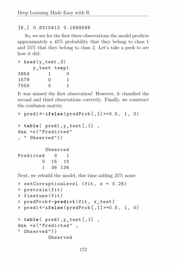
Deep Learning Made Easy with R
[6,] 0.8310412 0.1689588
So, we see for the first three observations the model predictsapproximately a 45% probability that they belong to class 1and 55% that they belong to class 2. Let’s take a peek to seehow it did:> head(y_test ,3)
y_test temp13954 1 01579 0 17000 0 1
It was missed the first observation! However, it classified thesecond and third observations correctly. Finally, we constructthe confusion matrix:> pred1 <-ifelse(predProb [,1]>=0.5, 1, 0)
> table( pred1 ,y_test[,1] ,dnn =c("Predicted", " Observed"))
ObservedPredicted 0 1
0 15 151 36 134
Next, we rebuild the model, this time adding 25% noise:> setCorruptionLevel (fit , x = 0.25)> pretrain(fit)> finetune(fit)> predProb <-predict(fit , x_test)> pred1 <-ifelse(predProb [,1]>=0.5, 1, 0)
> table( pred1 ,y_test[,1] ,dnn =c("Predicted" ," Observed"))
Observed
172

CHAPTER 6. THE STACKED AUTOENCODER IN . . .
Predicted 0 10 15 151 36 134
It appears to give us the same confusion matrix as a stackedautoencoder without any noise. So in this case, adding noisewas not of much benefit.
173

Deep Learning Made Easy with R
Notes101See Suwicha Jirayucharoensak, Setha Pan-Ngum, and Pasin Israsena,
“EEG-Based Emotion Recognition Using Deep Learning Network withPrincipal Component Based Covariate Shift Adaptation,” The Scien-tific World Journal, vol. 2014, Article ID 627892, 10 pages, 2014.doi:10.1155/2014/627892
102See G. E. Hinton, S. Osindero, and Y. W. Teh, “A fast learning al-gorithm for deep belief nets,” Neural Computation, vol. 18, no. 7, pp.1527–1554, 2006.
103See for example:Pugh, Justin K., Andrea Soltoggio, and Kenneth O. Stanley. "Real-
time hebbian learning from autoencoder features for control tasks." (2014).Cireşan, Dan, et al. "Multi-column deep neural network for traffic
sign classification." Neural Networks 32 (2012): 333-338.104Webb, W. B., and H. W. Agnew Jr. "Are we chronically sleep de-
prived?." Bulletin of the Psychonomic Society 6.1 (1975): 47-48.105Horne, James. Why we sleep: the functions of sleep in humans and
other mammals. Oxford University Press, 1988.106How Much Sleep Do You Really Need? By Laura Blue Friday, June
06, 2008.107Why Seven Hours of Sleep Might Be Better Than Eight by Sumathi
Reddy July 21, 2014.108Hirshkowitz, Max, et al. "National Sleep Foundation’s sleep time
duration recommendations: methodology and results summary." SleepHealth 1.1 (2015): 40-43.
109See http://www.aasmnet.org/110Tsinalis, Orestis, Paul M. Matthews, and Yike Guo. "Automatic Sleep
Stage Scoring Using Time-Frequency Analysis and Stacked Sparse Autoen-coders." Annals of biomedical engineering (2015): 1-11.
111See:
• Goldberger, Ary L., et al. "Physiobank, physiotoolkit, and phys-ionet components of a new research resource for complex physiologicsignals." Circulation 101.23 (2000): e215-e220.
• Also visit https://physionet.org/pn4/sleep-edfx/112See:
• Bengio, Yoshua, et al. "Greedy layer-wise training of deep net-works." Advances in neural information processing systems 19(2007): 153.
174

NOTES
• Vincent, Pascal, et al. "Extracting and composing robust featureswith denoising autoencoders." Proceedings of the 25th internationalconference on Machine learning. ACM, 2008.
113See Vincent, Pascal, et al. "Stacked denoising autoencoders: Learninguseful representations in a deep network with a local denoising criterion."The Journal of Machine Learning Research 11 (2010): 3371-3408.
114Möckel, Thomas, et al. "Classification of grassland successional stagesusing airborne hyperspectral imagery." Remote Sensing 6.8 (2014): 7732-7761.
115See Chen Xing, Li Ma, and Xiaoquan Yang, “Stacked Denoise Au-toencoder Based Feature Extraction and Classification for HyperspectralImages,” Journal of Sensors, vol. 2016, Article ID 3632943, 10 pages, 2016.doi:10.1155/2016/3632943
116Graham, Bell Alexander. "Improvement in telegraphy." U.S. PatentNo. 174,465. 7 Mar. 1876.
117Huq, N. and Cleland, J. (1990) Bangladesh Fertility Survey, 1989.Dhaka: National Institute of Population Research and Training (NI-PORT).
175

Deep Learning Made Easy with R
176

Chapter 7
Restricted BoltzmannMachines
We are drowning in information and starving forknowledge.Rutherford D. Roger
The Restricted Boltzmann Machine (RBM) is an unsu-pervised learning model that approximates the proba-bility density function of sample data. The “restricted”
part of the name points to the fact that there are no connec-tions between units in the same layer. The parameters of themodel are learned by maximizing the likelihood function of thesamples. Since it is used to approximate a probability densityfunction it is often referred to in the literature as a generativemodel118. Generative learning involves making guesses aboutthe probability distribution of the original input in order toreconstruct it.
The Four Steps to KnowledgeFigure 7.1 shows a graphical representation of an RBM. It iscomposed of two layers in which there are a number of units
177

Deep Learning Made Easy with R
with inner layer connections. Connections between layers aresymmetric and bidirectional, allowing information transfer inboth directions. It has one visible layer containing four nodesand one hidden layer containing three nodes. The visible nodesare related to the input attributes so that for each unit in thevisible layer, the corresponding attribute value is observable.
Figure 7.1: Graphical representation of an RBM model.
Here is an intuitive explanation, in four steps, of how they
178

CHAPTER 7. RESTRICTED BOLTZMANNMACHINES
work. Let’s consider the commonly used situation where allnodes (neurons/units) are binary. In this case:
1. Visible layer nodes take values vi = 0 or vi = 1.
2. Each node is a locus of computation that processes input,and begins by making stochastic decisions about whetherto transmit that input or not.
3. The hidden units serve to increase the expressiveness ofthe model and contain binary units where hj = 0 or hj =1.
4. For each unit or node in the hidden layer, the correspond-ing value is unobservable and it needs to be inferred.
The Role of Energy and ProbabilityThe RBM is a probabilistic energy-based model, meaning theprobability of a specific configuration of the visible and hiddenunits is proportional to the negative exponentiation of an en-ergy function, E(v, h). For each pair of a visible vector anda hidden vector the probability of the pair (v, h) is defined asfollows:
P (v, h) = 1Z
exp−E(v, h),
where the denominator Z is a normalizing constant known asthe partition function.
The partition function sums over all possible pairs of visibleand hidden variables is computed as:
Z =∑
v
∑h
exp−E(v, h),
It is therefore a normalizing constant such that P (v, h) definesa probability distribution over all possible pairs of v and h.
179

Deep Learning Made Easy with R
NOTE... �
A bipartite structure or graph is math speak for agroup of nodes which can only be one of two colors,with lines (edges) connecting the nodes (vertices)so that no two nodes of the same color are con-nected by a line. Figure 7.2 illustrates this idea.
Figure 7.2: Bipartite structure
In the RBM the bipartite graph is constructedof hidden and visible nodes as illustrated inFigure 7.1.
As there are no intra-layer connections within an RBM theenergy of a joint configuration (v, h), which defines a bipartite
180

CHAPTER 7. RESTRICTED BOLTZMANNMACHINES
structure, is given by:
E(v, h) = −m∑
i=1
n∑j=1
wijvihi −m∑
i=1vibi −
n∑j=1
hjdj,
where wij is the weight associated with the link between vi andhj. Intuitively, weights identify the correlation of the nodes.Larger weights imply a larger possibility that connected nodesconcur. The parameters bi and dj are the biases of the jthhidden and ith visible nodes respectively; and m and n are thenumber of nodes in the visible and hidden layer. Also notethat configurations with a lower energy function have a higherprobability of being realized.
A Magnificent Way to ThinkAnother way to think about a RBM is as a parametric modelof the joint probability distribution of visible and hidden vari-ables. It is therefore a type of autoencoder used to learn arepresentation (encoding) in terms of the joint probability dis-tribution for a set of data.
Since the hidden units of the RBM only connect to unitsoutside of their specific layer, they are mutually independentgiven the visible units. The conditional independence of theunits in the same layer is a nice property because it allows usto factorize the conditional distributions of the hidden unitsgiven the visible units as:
P (h|v) =∏j
P (hj|v),
with
P (hj = 1|v) =∏j
sigmoid
(∑i
wijvi + dj
)
181

Deep Learning Made Easy with R
The conditional distribution of the visible units can be factor-ized in a similar way:
P (v|h) =∏
i
P (vi|h),
with
P (vi = 1|h) =∏
i
sigmoid
∑j
wijhj + bi
These conditional probabilities are important for the iterativeupdates between hidden and visible layers when training anRBM model. In practice, Z is difficult to calculate so compu-tation of the joint distribution P (v, h) is typically intractable.
NOTE... �
Notice that RBMs have two biases. This is oneaspect that distinguishes them from other autoen-coders. The hidden bias dj helps the RBM pro-duce the activations on the forward pass throughthe network, while the visible layer’s biases bi helpthe RBM learn the reconstructions during back-propagation or the backward pass.
The Goal of Model LearningThe goal in training an RBM is to adjust the parameters of themodel, denoted by Θ, so that the log-likelihood function usingthe training data is maximized.
The gradient of the log-likelihood is:
∂
∂ΘL(Θ) = −⟨∂E(v; Θ)∂Θ
⟩data
+⟨∂E(v; Θ)∂Θ
⟩model
182

CHAPTER 7. RESTRICTED BOLTZMANNMACHINES
where 〈•〉data represents the expectation of all visible nodesv in regard to the data distribution and 〈•〉model denotes themodel joint distribution defined by P (v, h).Rather unfortunately the log-likelihood gradient is difficult tocompute because it involves the intractable partition functionZ. To solve this issue, we need a trick. Fortunately, datascience has one at hand.
Training Tricks that Work Like MagicThe first training trick involves use of the expressions for P (h|v)and P (v|h). Since both of these expressions are tractable whynot use them to sample from the joint distribution P (v, h) usinga Gibbs sampler?
Trick 1: O Jogo Bonito!Gibbs sampling is a Monte Carlo Markov chain algorithm forproducing samples from the joint probability distribution ofmultiple random variables. The basic idea is to construct aMarkov chain by updating each variable based on its condi-tional distribution given the state of the others. This turnsout to be a great idea, it involves fancy footwork even Pelé, themost successful league goal scorer in the history of the beautifulgame, would be proud - O Jogo Bonito!
In Gibbs sampling the visible nodes are sampled simultane-ously given fixed values of the hidden nodes. Similarly, hiddennodes are sampled simultaneously given the visible nodes. Foreach step in the Markov chain the hidden layer units are ran-domly chosen to be either 1 or 0 with probability determinedby their sigmoid function; and similarly the visible layer unitare randomly chosen to be either 1 or 0 with probability deter-mined by their sigmoid function.
As the number of steps becomes infinitely large the sam-ples of the hidden and visible nodes converge to the joint dis-
183

Deep Learning Made Easy with R
tribution P (v, h). Through this rather neat trick stochasticestimates of the gradient are easily obtained.
When I say” easily”, take it with a “pinch of salt.” If youare in a hurry, the results were due yesterday, the boss or theclient or (heaven forbid) reporters are foaming at the mouthbaying for results, then this type of “easy” won’t work for you.This is because one iteration of alternating Gibbs samplingrequires updating all of the hidden units in parallel for P (h|v),followed by updating all of the visible units in parallel P (v|h).Gibbs sampling therefore can take a very long time to converge.Depending on your need for speed, it may be totally unfeasiblefor your data science challenge.
So you may wonder, what type of trick is this? Maybe it islike the magician who saws the beautiful women in half, andthen later in the show she reappears smiling and waving andtotally “together”. I’m amazed every time I see that particulartrick. But of what real practical use is it?
Well hang on just a moment! There is another trick thatgoes along with the first trick. In fact, the second trick su-percharges the first trick. If you only had the first trick youmight be satisfied, and many Statisticians were. Maybe, if youfind yourself with code to write, you would keep it in yourback pocket for smallish datasets. In fact, you might use itso infrequently as to forget about it entirely! However, withthis second trick in hand you have the keys to the RestrictedBoltzmann Machine Kingdom (metaphorically speaking).
Trick 2: The Keys to the KingdomHere is the second trick - contrastive divergence which mini-mizes the Kullback–Leibler distance (see page 126). We won’tgo into all of the technical details, but at the core is this idea- Start the Markov chain by setting the states of the visibleunits to a training vector. Then the binary states of the hid-den units are all computed in parallel to calculate P (h|v). Oncethe binary states have been chosen for the hidden units, a “re-
184

CHAPTER 7. RESTRICTED BOLTZMANNMACHINES
construction" is produced by setting each vi to 1 with a prob-ability given by P (v|h). Now run Gibbs sampling for a verysmall number of iterations, but don’t wait for convergence.
If we use k to denote the number of Gibbs sampling itera-tions, then k=1 will do the job for many applications! Yes, inmany applications you only need run the Gibbs sampler for 1step. Since 1 is a lot less than infinity this saves a lot of time! Insummary, sampling k (usually k = 1) steps from a Gibbs chaininitialized with a data sample yields the contrastive divergence.
In practice more efficiencies are available because updatesare typically performed using multiple training examples at atime by averaging over the updates produced by each example.This smooths the learning signal and also helps take advantageof the efficiency of larger matrix operations.
Using the Gibbs sample, the observed data and the free en-ergy function119; we are able to approximate the log likelihoodgradient. This used in conjunction with the gradient descentback propagation algorithm allows the log likelihood estimatesΘ to be efficiently obtained.
Trick 3: Back Pocket Activation’sThe standard RBM model uses binary units (BU) in both thevisible and hidden layers with the sigmoid activation function.However, many other types of activation can also be used. Inparticular, real valued data in the range of [0-1] can be modeledusing a logistic activation function and contrastive divergencetraining without any modification.
Another popular activity function are the rectified linearunits (see page 18). Vinod and Hinton report120 rectified linearunits (RLU) demonstrate strong results for image analysis. Onone task using 32 × 32 color images, the researchers reportthe RLU had a prediction accuracy of 0.8073 compared to aprediction accuracy of 0.7777 for BU. However, the standarddeviations were too large for the difference to be statisticallysignificant.
185

Deep Learning Made Easy with R
Another advantage of the RLU is that they do not havemore parameters than the BU, but they are much more ex-pressive. As Vinod and Hinton state “Compared with binaryunits, these units [RLUs] learn features that are better for objectrecognition on the NORB dataset121 and face verification onthe Labeled Faces in the Wild dataset122. Unlike binary units,rectified linear units preserve information about relative inten-sities as information travels through multiple layers of featuredetectors.”
Trick 4: Alternatives to Contrastive Diver-genceSince an RBM defines a distribution over all of its variables,there is more than one strategy that can be used to train it.This is good for you because the art of data science lies infinding useful alternatives.
Persistent contrastive divergence is one such alternative. Ituses another approximation for sampling from p(v, h) that re-lies on a single Markov chain which has a persistent state123,where the Markov chain is not reinitialized with a data sampleafter parameter updates. It uses the last chain state in thelast update step. This technique has been reported to lead tobetter gradient approximations if the learning rate is chosensufficiently small.
Fast Persistent Contrastive Divergence124 is another variantwhich attempts to speed up learning by introducing an addi-tional set of parameters used only for Gibbs sampling procedureduring learning.
Parallel Tempering125, also known as Replica ExchangeMonte Carlo Markov Chain sampling, is another technique youmight stumble across. The general idea of parallel temperingis to simulate replicas of the original system of interest by in-troducing supplementary Gibbs chains.
Each replica is typically at a different temperature. Thehigher the temperature, the ‘smoother’ the corresponding dis-
186

CHAPTER 7. RESTRICTED BOLTZMANNMACHINES
tribution of the chain. Parallel tempering leads to better mix-ing of the original chain (i.e. achieves good sampling) by al-lowing the systems at different temperatures to exchange com-plete configurations with a probability given by the MetropolisHastings ratio. It turns out that the simulation of K replicasis more than 1/K times more efficient than a standard, single-temperature Monte Carlo simulation. One additional advan-tage of this technique is that it can make efficient use of largeCPU clusters, where different replicas can be run in parallel.
The Key Criticism of Deep LearningWhy does the contrastive divergence approach work? I don’tknow. The best I can tell you is that the theoreticians don’tknow either! Scholars Sutskever and Tieleman126 pointed outdecisively that the learning rule is not following the gradientof any function whatsoever. They state “Despite CD’s [con-trastive divergence’s] empirical success, little is known about itstheoretical convergence properties.” As Boston University Pro-fessor of Physics Pankaj Mehta and Northwestern UniversityProfessor of biological physics David Schwab point out aboutdeep learning127 “Despite the enormous success of deep learn-ing, relatively little is understood theoretically about why thesetechniques are so successful at feature learning and compres-sion.”
A key criticism of deep learning is that the theoretical prop-erties of the methods introduced, for example contrastive di-vergence, are not well understood; And this is absolutely cor-rect. But is this a problem? Hell, no! The most successfuldata scientists are pragmatic. They run well ahead of the the-oreticians and innovate solutions to practical problems. Theyleave the theoreticians several steps behind gasping for breathwrestling with the “why” question. If a technique works out-standingly well data scientists use it until something betteris discovered. The contrastive divergence approach works well
187

Deep Learning Made Easy with R
enough to achieve success in many significant applications. The“why”, although interesting, can wait!
Did Alexander Graham Bell understand completely thephysics of his "apparatus for transmitting vocal or other soundstelegraphically"? No! But he made a financial fortune, changedthe world and went down in history as one of the great in-ventors of his era. What about University College, London,professor of mathematics Karl Pearson? Back in 1901 did heunderstand totally and completely the theoretical properties ofhis very practical principal component analysis statistical tool?Does the machine learning Guru, Professor Hinton128 who dis-covered contrastive divergence, understand all of its theoreticalnuances?
Once the theoreticians catch up, they provide additionalsupport for why a great idea is a great idea. And this is avery important activity. But we can’t wait for them, let’s keeprunning!
Two Ideas that can Change the WorldIn the past decade, the restricted Boltzmann machine (RBM)had been widely used in many applications including dimen-sionality reduction, classification, collaborative filtering, fea-ture learning, and topic modeling. In this section we exploretwo very promising ideas, which each in their own way, canchange the world.
How to Punch Cancer in the FaceSeveral years ago voice-over artist, writer and actress EricaMcMaster, an Ottawa native, began to train as a fighter. Hermind was so focused and her determination so complete thather training activities captured the imagination of the localpress. At the end of a beautiful spring day in the historicOld Mill Inn in Etobicoke, adjacent to Toronto’s gentle flowing
188

CHAPTER 7. RESTRICTED BOLTZMANNMACHINES
Humber river and luscious parkland, Erica climbed into theboxing ring and let her fists do the talking.
Her opponent was cancer, and her goal: “To punch cancerin the face.” Erica lost her mother, two of her grandparentsand a childhood friend to the disease. The Princess MargaretCancer Foundation’s Annual Fight To End Cancer Fundraiserwas a huge success129.
Whilst very few data scientists are trained fighters, the toolswe wield can, and do save lives. Let’s look at one example ofhow deep learning can help Erica McMaster “Punch cancer inthe face.”
Clinical researchers have demonstrated conclusively thatcancer sera contain antibodies which react with a unique groupof autologous cellular antigens called tumor-associated anti-gens130. This is exciting news because mini-arrays of antigenshave the potential to detect and diagnose various types of can-cer. The trick is to associate the correct combination of anti-gens with a specific type of cancer. Once the mini-arrays havebeen created, this becomes a classification problem for whichRBM’s are well suited RBM.
Koziol et al.131 examine the use of RBMs for the classifica-tion of Hepatocellular Carcinoma132. The standard approachto such classification is logistic regression. It is the grandsonof linear regression, a member of the generalized linear familyof models and has reigned supreme in the medical statisticscommunity for several decades.
It appears the logistic model was first introduced sometimeduring the first half of the 19th century by statistician AlphonseQuetlet’s student Pierre-François Verhulst. It was discovered,in part, as an exercise to moderate Thomas Malthus’s expo-nential population growth model. Close to 200 years after Ver-hulst’s discovery, the scientific community, commercial sectorsand government researchers have fully embraced it as a viabletool for binary data.
Since it is based on modeling the odds of an outcome itis perfectly suited to the classification task, and has rightly
189

Deep Learning Made Easy with R
earned its place as the gold standard in many disciplines. Takefor example, the United Kingdom, where the performance oftrauma departments is widely audited by applying predictivemodels that assess the probability of survival, and examiningthe rate of unexpected survivals and deaths.
The standard approach is the TRISS133 methodology, in-troduced in 1981. It is a standardized approach for trackingand evaluating outcome of trauma care and is calculated as acombination index based on the revised trauma score (RTS),injury severity score (ISS) and patient’s age. TRISS determinesthe probability of survival of a patient from two logistic regres-sions, one applied if the patient has a penetrating injury andthe other applied for blunt injuries134.
Today logistic regression is one of the most widely taughtand used binary models in the analysis of categorical data. Itis a staple in statistics 101 classes, dominates quantitative mar-keting, and is used with numerous mutations in classical econo-metrics135. You may have studied it and explored its power inyour own research. If not, add it to your tool kit today!136 Innumerous areas it has become the benchmark which challengermodels must meet and defeat.
For their comparative study of logistic regression and RBMKoziol et al. collected sera samples from 175 HepatocellularCarcinoma patients and 90 normal patients. Twelve antigenswere expressed as recombinant proteins. The researchers used a10-fold cross-validation for both the RBM and logistic regres-sion models. The entire data set was randomly divided into10 equally sized sub-samples. With each sub-sample stratifiedto preserve the ratio of cancer cases to controls. The logisticregression and RBM were trained on 9 sub-samples; the 10thsample was used for validation.
190

CHAPTER 7. RESTRICTED BOLTZMANNMACHINES
NOTE... �
Sensitivity is the ability of a classifier to identifypositive results, while specificity is the ability todistinguish negative results.
Sensitivity = NTP
NTP +NTN× 100 (7.1)
Specificity = NTN
NTP +NTN× 100 (7.2)
NTP is the number of true positives and NTN isthe number of true negatives.
The results for dichotomized data using 12 antigens areshown in Table 7. These results, although promising, are cer-tainly not a home run for RBM; and this is to be expectedbecause data science is all about obtaining a slight edge. Itis all you need to win. If data scientists like you can developmodels which give us a slight edge over cancer, we will be wellon the way to “punching it in the face.”
Koziol et al.conclude tentatively “Their relatively good per-formance in our classification problem is promising, and RBMsmerit further consideration in similar investigations. We en-courage others to explore further the utility of the RBM ap-proach in similar settings.” Other researcher will perform followup studies, maybe even you?
A Magnificent Way to Assist the AnaesthetistJust prior to writing this book I found myself hospitalized. Iwas barely able to walk and rushed into the emergency ward.Within a matter of minutes, the medical professionals diag-nosed my issue and began to stabilize my biological metrics.
191

Deep Learning Made Easy with R
Model Sensitivity SpecificityLogistic Regression 0.697 0.811RBM 0.720 0.800
Table 7: Results for dichotomized data using 12 antigens.Source Koziol et al.
The very next day I went into surgery, the last thing I recallwas the Anaesthetist administrating general anaesthesia.
Surgery lasted twenty minutes, I awoke groggy, pain freeand quickly recovered. The incident got me thinking, wouldn’tit be an amazing if data science techniques could assist moni-toring and administrating of general anaesthesia?
Professor of bio medical engineering, bio-signal processing,medical ultrasound and meditronics, Pei-Jarn Chen and asso-ciates137 had a similar idea.
The researchers develop a RBM to predict the depth ofsedation using biological signals as input attributes/ features.Two distinct types of features are extracted.
The first group of attributes were related to a patient’s auto-nomic nervous system which regulates the functions of internalorgans such as the heart, stomach and intestines. They includethe heart rate, blood pressure and peripheral capillary oxygensaturation (SpO2).
The second group of attributes measured metrics relatedto the patient’s state induced by an anesthesia. This includedthe fractional anesthetic concentration, end-tidal carbon diox-ide138, fraction inspiration carbon dioxide139, and minimumalveolar concentration140.
192

CHAPTER 7. RESTRICTED BOLTZMANNMACHINES
NOTE... �
Cross-validation refers to a technique used to allowfor the training and testing of inductive models.Leave-one-out cross-validation involves taking outone observation from your sample and training themodel with the rest. The predictor just trainedis applied to the excluded observation. One oftwo possibilities will occur: the predictor is cor-rect on the previously unseen control, or not. Theremoved observation is then returned, and the nextobservation is removed, and again training andtesting are done. This process is repeated for allobservations. When this is completed, the resultsare used to calculate the accuracy of the model.
Continuous data, including the response variable depth ofsedation, was collected on 27 patients subject to anaesthesia.The training set consisted of 5000 randomly selected epochsand 1000 epochs for the sample. Leave one- out cross-validationwith the mean square error (MSE) was used to evaluate per-formance.
As a benchmark for performance the researchers comparedthe MSE of the RBM model to a feed-forward neural network(ANN) and modular neural networks using different features(MN–1, MN–2,MN–3).
Figure 7.3 illustrates the results. It shows the average MSEfor ANN,MN–1, MN–2,MN–3, and RBM model. The MSEwere 0.0665, 0.0590, 0.0551, 0.0515, and 0.0504, respectively.The RBM model has the smallest error. This is a positive signfor the use of RBM, although not conclusive because the MSEappears to be statistically indistinguishable from that of MN–3.
Chen et al. are slightly bolder than I am (wearing my statis-tician hat), and assert “The experimental results demonstrated
193

Deep Learning Made Easy with R
that the proposed approach outperforms feed-forward neural net-work and modular neural network. Therefore, the proposedapproach is able to ease patient monitoring services by usingbiological systems and promote healthcare quality.” ProfessorChen’s research is a clear step forward. This is an excitingtime to be involved in data science!
Figure 7.3: MSE results of different modeling approaches.Source adapted from Chen et al. cited in endnote sec. 137
Secrets to the Restricted BoltzmannMachine in RLet’s build an RBM using the Mobility dataframe discussedpreviously on page 166. First we load the required packagesand data:>require(RcppDL)> require("ltm")> data(Mobility)> data <-Mobility
194

CHAPTER 7. RESTRICTED BOLTZMANNMACHINES
The package RcppDL contains functions to estimate a RBM.The package ltm contains the Mobility dataset.
We sample 1000 observations for our analysis, using 800 forthe training set:> set.seed (2395)> n=nrow(data)> sample <- sample (1:n, 1000, FALSE)> data <-as.matrix(Mobility[sample ,])> n=nrow(data)> train <- sample (1:n, 800, FALSE)
Now create the train and test attribute objects in R(x_train,x_test). For this example we will remove item 4and item 6 from the sample (see Table 6):> x_train <-matrix(as.numeric(unlist(data[
train ,])),nrow=nrow(data[train ,]))> x_test<-matrix(as.numeric(unlist(data[-
train ,])),nrow=nrow(data[-train ,]))
> x_train <-x_train[,-c(4,6)]> x_test<-x_test[,-c(4,6)]
> head(x_train)[,1] [,2] [,3] [,4] [,5] [,6]
[1,] 1 1 1 1 0 1[2,] 1 0 1 0 0 0[3,] 1 1 1 0 0 0[4,] 1 0 0 0 0 0[5,] 1 0 0 0 0 0[6,] 1 1 1 0 0 0> head(x_test)
[,1] [,2] [,3] [,4] [,5] [,6][1,] 0 0 0 0 0 0[2,] 1 0 0 0 0 0[3,] 1 0 0 0 0 0[4,] 1 0 1 0 0 0
195

Deep Learning Made Easy with R
[5,] 1 1 1 1 0 0[6,] 0 0 1 0 0 0
Specification of the model is similar to what we have previ-ously seen:> fit <- Rrbm(x_train)
The r object fit contains the model specification. We set 3hidden nodes with a learning rate of 0.01:> setHiddenRepresentation (fit , x = 3)> setLearningRate(fit , x = 0.01)
Here is the summary of the model:> summary(fit)$LearningRate[1] 0.01
$ContrastiveDivergenceStep[1] 1
$TrainingEpochs[1] 1000
$HiddenRepresentation[1] 3
Now the parameters have been selected, training is achievedusing:> train(fit)
That’s it! We have built a RBM.
196

CHAPTER 7. RESTRICTED BOLTZMANNMACHINES
NOTE... �
You can set a number of the parameters in Rrbmincluding:
• setStep signature
• setHiddenRepresentation
• setLearningRate
• setTrainingEpochs
Now, let’s see if we can reconstruct the original values in asimilar way to what we did in chapter 5. To achieve this use thereconstruct function to obtain the estimated probabilities:reconProb <-reconstruct(fit ,x_train)
Then convert the probabilities into binary values:> recon <-ifelse(reconProb >=0.5 , 1, 0)
You should now see the reconstructed values something likethis:> head(recon)
[,1] [,2] [,3] [,4] [,5] [,6][1,] 1 0 1 0 0 0[2,] 1 0 1 0 0 0
197

Deep Learning Made Easy with R
[3,] 1 0 1 0 0 0[4,] 1 0 1 0 0 0[5,] 1 0 1 0 0 0[6,] 1 0 1 0 0 0
Finally, we can create a global confusion matrix for all sixattributes combined:> table( recon ,x_train , dnn =c("Predicted"
, " Observed"))Observed
Predicted 0 10 2786 4141 371 1229
It can also be useful to view an image of the reconstructedvalues as shown in Figure 7.4. This is achieved by:> par( mfrow =c(1, 2))> image(x_train ,main="Train")> image(recon ,main="Reconstruction")
The reconstructed image appears to contain the main block likefeatures, although not the finer details in terms of streakingacross the major blocks. It is left as an exercise for the readerto further refine and improve the model.
198

CHAPTER 7. RESTRICTED BOLTZMANNMACHINES
Figure 7.4: RBM train set and reconstructed values usingMobility
199

Deep Learning Made Easy with R
NOTE... �
You can also estimate a RBM with the deepnetpackage. Here is how to do that:> fit2<-rbm.train(x_train ,+ hidden=3,+ numepochs = 3,+ batchsize = 100,+ learningrate = 0.8,+ learningrate_scale = 1,+ momentum = 0.5,+ visible_type = "bin",+ hidden_type = "bin",+ cd = 1)
Much of this should be familiar to you. Noticethat rbm.train allows you to specify the batch sizewhich is useful in very large samples. the parame-ter cd refers to the number of steps for contrastivedivergence (see sec. 7).
RBMs are powerful learning machines in their own right,however arguably their most important use is as learning mod-ules used in the construction of deep belief networks; and thatis the subject of the next chapter.
200

NOTES
Notes118A RBM is a bipartite Markov random field.119Unless you are writing computer code to calculate the estimates, the
specific details of the algorithm are less important than an intuitive un-derstanding. However,
• A detailed description which is very easy to follow can be found inBengio, Yoshua. "Learning deep architectures for AI." Foundationsand trends® in Machine Learning 2.1 (2009): 1-127.
• Another easy to follow guide is Hinton, Geoffrey. "A practical guideto training restricted Boltzmann machines." Momentum 9.1 (2010):926.
• If you would like additional details on how contrastive divergenceworks you can email me at info@NigelDLewis. I’d be delighted toshare updated resources with you.
120Nair, Vinod, and Geoffrey E. Hinton. "Rectified linear units improverestricted boltzmann machines." Proceedings of the 27th InternationalConference on Machine Learning (ICML-10). 2010.
121A dataset which contains images of 50 toys belonging to 5 genericcategories: four-legged animals, human figures, airplanes, trucks, and cars.The objects were imaged by two cameras under 6 lighting conditions, 9elevations, and 18 azimuths. For further details please see: LeCun, Yann,Fu Jie Huang, and Leon Bottou. "Learning methods for generic objectrecognition with invariance to pose and lighting." Computer Vision andPattern Recognition, 2004. CVPR 2004. Proceedings of the 2004 IEEEComputer Society Conference on. Vol. 2. IEEE, 2004.
122A database of face photographs designed for studying the problem ofunconstrained face recognition. The data set contains more than 13,000images of faces collected from the web. For further details please seeGary B. Huang, Manu Ramesh, Tamara Berg, and Erik Learned-Miller.Labeled Faces in the Wild: A Database for Studying Face Recognitionin Unconstrained Environments. University of Massachusetts, Amherst,Technical Report 07-49, October, 2007.
123For details see Tieleman, Tijmen. "Training restricted Boltzmannmachines using approximations to the likelihood gradient." Proceedings ofthe 25th international conference on Machine learning. ACM, 2008.
124Tieleman, Tijmen, and Geoffrey Hinton. "Using fast weights to im-prove persistent contrastive divergence." Proceedings of the 26th AnnualInternational Conference on Machine Learning. ACM, 2009.
125See:
201

Deep Learning Made Easy with R
• C. J. Geyer, in Computing Science and Statistics Proceedings of the23rd Symposium on the Interface, American Statistical Association,New York, 1991, p. 156.
• Cho, KyungHyun, Tapani Raiko, and Alexander Ilin. "Paralleltempering is efficient for learning restricted Boltzmann machines."IJCNN. 2010.
• Fischer, Asja, and Christian Igel. "A bound for the convergence rateof parallel tempering for sampling restricted Boltzmann machines."Theoretical Computer Science (2015).
126
• See Sutskever, Ilya, and Tijmen Tieleman. "On the convergenceproperties of contrastive divergence." International Conference onArtificial Intelligence and Statistics. 2010.
• Also note that the observation that the contrastive divergence up-date is not the gradient of any objective function was first provedby university of Toronto student Tijmen. See: Some investigationsinto energy based models. Master’s thesis, University of Toronto.
127Mehta, Pankaj, and David J. Schwab. "An exact mapping betweenthe variational renormalization group and deep learning." arXiv preprintarXiv:1410.3831 (2014).
128Hinton, Geoffrey E. "Training products of experts by minimizing con-trastive divergence." Neural computation 14.8 (2002): 1771-1800.
129See Toronto Sun article ’Punch cancer in the face’ by Steve Buffery.Sunday, March 08, 2015.
130See for example:
• Liu, W., et al. "Evaluation of Tumour Associated Antigen (TAA)Miniarray in Immunodiagnosis of Colon Cancer." Scandinavianjournal of immunology 69.1 (2009): 57-63.
• Tan, Hwee Tong, et al. "Serum autoantibodies as biomarkers forearly cancer detection." FEBS journal 276.23 (2009): 6880-6904.
• Ye, Hua, et al. "Mini-array of multiple tumor-associated antigens(TAAs) in the immunodiagnosis of breast cancer." Oncology letters5.2 (2013): 663-668.
• Coronell, Johana A. Luna, et al. "The current status of cancerbiomarker research using tumour-associated antigens for minimalinvasive and early cancer diagnostics." Journal of proteomics 76(2012): 102-115.
202

NOTES
131James A. Koziol, Eng M. Tan, Liping Dai, Pengfei Ren, and Jian-YingZhang, “Restricted Boltzmann Machines for Classification of Hepatocel-lular Carcinoma,” Computational Biology Journal, vol. 2014, Article ID418069, 5 pages, 2014. doi:10.1155/2014/418069
132 Liver cancer133see:
• Champion, Howard R., et al. "Trauma score." Critical caremedicine 9.9 (1981): 672-676.
• Champion, Howard R., et al. "A revision of the Trauma Score."Journal of Trauma and Acute Care Surgery 29.5 (1989): 623-629.
• H.R. Champion et.al, Improved Predictions from a Severity Char-acterization of Trauma (ASCOT) over Trauma and Injury SeverityScore (TRISS): Results of an Independent Evaluation. Journal ofTrauma: Injury, Infection and Critical Care, 40 (1), 1996.
134To try out TRISS for yourself visit http://www.trauma.org/index.php/main/article/387/
135See for example Maddala’s book. Add it to your personal library. Itis a classic and worth every penny:
• Maddala, Gangadharrao S. Limited-dependent and qualitative vari-ables in econometrics. No. 3. Cambridge university press, 1986.
136To get you started, here are five books that will tell you all you needto know as a data scientist:
• Allison, Paul D. Logistic regression using SAS: Theory and appli-cation. SAS Institute, 2012.
• Harrell, Frank E. Regression modeling strategies: with applicationsto linear models, logistic regression, and survival analysis. SpringerScience & Business Media, 2013.
• Hosmer Jr, David W., Stanley Lemeshow, and Rodney X. Sturdi-vant. Applied logistic regression. Vol. 398. John Wiley & Sons,2013.
• Menard, Scott. Applied logistic regression analysis. Vol. 106. Sage,2002.
• Kleinbaum, David G., and Mitchel Klein. Analysis of MatchedData Using Logistic Regression. Springer New York, 2010.
137Yeou-Jiunn Chen, Shih-Chung Chen, and Pei-Jarn Chen, “Predictionof Depth of Sedation from Biological Signals Using Continuous RestrictedBoltzmann Machine,” Mathematical Problems in Engineering, vol. 2014,Article ID 189040, 6 pages, 2014. doi:10.1155/2014/189040
203

Deep Learning Made Easy with R
138Measurement of exhaled carbon dioxide.139The fraction or percentage of oxygen in the space being measured. It is
used to represent the percentage of oxygen participating in gas-exchange.140The concentration of vapor in the lungs that is required to prevent
movement in half of subjects in response to surgical stimulus.
204

Chapter 8
Deep Belief Networks
Statisticians, like artists, have the bad habit offalling in love with their models.George Box
A deep belief network (DBN) is a probabilistic generativemultilayer neural network composed of several stackedRestricted Boltzmann Machines. In a DBN, every two
sequential hidden neural layers form an RBM. The input ofthe current RBM is actually the output features of a previousone. Each model performs a nonlinear transformation on itsinput vectors and produces as output, the vectors that will beused as input for the next model in the sequence. Thus eachRBM in the stack that makes up a DBN receives a differentrepresentation of the data.
DBNs usually consists of two types of layer. They are visiblelayer and hidden layer. Visible layers contain input nodes andoutput nodes, and hidden layers contain hidden nodes. Thetraining of DBN can be divided into two steps: pretrainingand fine-tuning using discriminative backpropagation.
205

Deep Learning Made Easy with R
How to Train a Deep Belief NetworkPre-training followed by fine tuning is a powerful mechanismfor training a deep belief networks141. Let’s take a look at eachof these elements.
The Key Elements of Pre-trainingPre-training helps generalization; it uses a layer-wise greedylearning strategy in which each RBM is trained individuallylayer by layer using contrastive divergence and then stacked ontop of each other.
When the first RBM has been trained, its parameters arefixed, and the hidden unit values are used as the visible unitvalues for the second RBM. This is done by training it using thetraining sample as the visible layer. Then weights of the learnedRBM are then used to predict the probability of activating thehidden nodes for each example in the training dataset.
These activation probabilities are then used as the visiblelayer in the second RBM. This procedure is repeated severaltimes to initialize the weights for several hidden layers untilthe final RBM is trained. Overall, the DBN, as with othermultilayer neural networks, can be efficiently trained by usingthe feature activation’s of one layer as the training data for thenext.
Since pretraining is unsupervised, no class labels are re-quired at this stage. In practice a batch-learning method isoften applied to accelerate the pre-training process with theweights of the RBMs updated every mini-batch.
The many layers of hidden units create many layers of fea-ture detectors that become progressively more complex. Pre-training is believed to help capture high level features of thedata which assist supervised learning when labels are providedin the fine tuning stage.
206

CHAPTER 8. DEEP BELIEF NETWORKS
The Heart of Fine-tuningThe fine-tuning stage uses the standard back-propagation al-gorithm through the whole pre-trained network to adjust thefeatures in every layer to make them more useful for classifi-cation. This, as we have seen earlier, involves adjusting theweights for enhanced discriminative ability by minimizing theerror between the network predicted class and the actual class.
A softmax output layer is typical used as a multiclass classi-fier. The softmax classifier therefore learns a joint model of thefeatures extracted by the RBMs and the corresponding labelof the test samples where the number of nodes in the outputlayer is equal to the number of classes.
Since fine-tuning involves supervised learning, the corre-sponding labels for the training data are needed. After training,the predicted class label of a test sample are obtained in theusual manner - by propagation of the test data forward fromthe first layer visible through to the softmax output layer.
How to Deliver a Better Call WaitingExperienceCall routing is the task of getting callers to the right place inthe call center, which could be the appropriate live agent orautomated service. Several years ago this was thought bestachieved with a list of menu options for callers to select us-ing a telephone touch-tone keypad. These menu drive systemshave provided comedians with a goldmine of funny material. Imyself have been frustrated, baffled and annoyed on many oc-casions trying to navigate through menu driven systems. GlynRichard’s YouTube video captures the real world experience ofmany142.
Imagine my joy when telecommunications giant VerizonCorporate Services Group Inc. filed patent number US7092888B1 - Unsupervised training in natural language call routing143.
207

Deep Learning Made Easy with R
Natural language call routing allows callers to describe the rea-son for their call in their own words, instead of presenting themwith a frustrating and limiting menu!
Well over a decade has passed since the original filing date.Over that time, we have seen a steady rise in natural languagecall routing. Alas, purely menu driven systems are still withus!
Deep learning has an important role to play in this space.IBM researcher Ruhi Sarikaya144 investigated the role of DBNsin natural language call routing. This is a very interesting ap-plication because it involves real time data collected from acustomer call center for a Fortune 500 company. Such compa-nies typically have a wide variety of call types to deal with andthe call–routing system for this particular company is coded torespond to 35 different call types.
The training sample consisted of 27,000 automatically tran-scribed utterances amounting to 178,000 words in total. In or-der to assess the impact of data size on learning method, Ruhidivided the sample into a range of sets from 1,000 to 10,000and also included the original sample size of 27,000.
Pre-training was achieved with contrastive divergence. Themodel was fine-tuned with backpropagation (stochastic gradi-ent descent) using an early stopping rule (see page 57) whichlimited the number of iterations to 100.
Ruhi reports that the performance improved as the sampledata was increased from 1,000 to 10,000. For example, thereported prediction accuracy was 78.1% for the smallest samplesize of 1,000, 87% for the sample size of 6,000, and 90.3% forthe full sample of 27,000.
In line with data science best practice Ruhi used a range ofalternative data analytic models as benchmarks, including thesupport vector machine (SVM). Ruhi and collaborators con-clude by stating “DBNs performed as well as or slightly betterthan SVMs for all sizes of training set.”
208

CHAPTER 8. DEEP BELIEF NETWORKS
A World First Idea that You Can Eas-ily EmulateMany longstanding residents of the Great State of Texas canstill recall the drought of 1949 to 1956. Ask them, and theywill tell you how Lake Dallas shrunk down to 1/10 of its size,and how west of the Pecos River only eight inches of rain wasrecorded for the entire year of 1953. Of course the droughtended, as all droughts do with a deluge of rain that soaked theentire state in the spring of 1956.
I often recount my own memories of the Great Drought of75 and 76 in England, where hot weather dried up lakes and re-sulted in water restrictions. It was reported as the hottest sum-mer average temperature in the United Kingdom since recordsbegan. And since the British have kept records since at least1066, that is a dam long time! It too ended in a deluge of rainin the autumn of 76.
Now here is the interesting thing, data scientists have beenattempting to predict drought conditions, since before statis-tics was considered a formal scientific discipline. Governments,local authorities and regional water boards would all like toknow when drought conditions are likely to occur.
Researchers Junfei Chen, Qiongji Jin of Hohai universityand Jing Chao of Nanjing university investigate this issue usingDBNs. Collectively, they have developed what appears to bethe worlds first short-term drought prediction model based ondeep belief networks145. The goal of the researchers was toinvestigate whether DBNs can be used to predict drought inthe Huaihe River Basin.
Data on monthly rainfall from four hydrologic stations(Bengbu, Fuyang, Xuchang, and Zhumadian) was collectedfrom January 1958 to 2006 and then transformed into differ-ent time scales using the Standardized Precipitation Index146(SPI). SPI is an index used to characterize meteorologicaldrought on a range of timescales. On short timescales, the SPI
209

Deep Learning Made Easy with R
is closely related to soil moisture, while at longer timescales,the SPI can be related to groundwater and reservoir storage.
Four timescales were used by the researchers SPI3, SPI6,SPI9, and SPI12. The training sample consisted of data fromthe period 1958–1999, and the testing sample used observationsfrom 2000–2006.
A total of 16 DBN models were developed, one for each siteand SPI index. The optimal number of nodes in each modelis given in Table 8. We see, for example, the DBN developedusing the SP13 series at the Bengbu measuring station has 9input nodes, 5 hidden nodes in the first layer, and 10 hiddennodes in the second layer. Whilst the DBN for SPI12 for thesame weather station has 8 input nodes, with 5 nodes in eachof the hidden layers.
Table 8: The optimal network structures of DBN. Source oftable Chen et al. cited in endnote sec. 145.
Figure 8.1 illustrates the fit of the DBN models for theBengbu measuring station. Visually, the fit of each model looksreasonable. The root mean square error (RMSE) and mean ab-solute error (MAE) are also given.
210

CHAPTER 8. DEEP BELIEF NETWORKS
The researchers benchmark their models against a back-propagation (BP) neural network and find the DBN clearly out-performs. This leads them to conclude “The errors results showthat the DBN model outperforms the BP neural network. Thisstudy shows that the DBN model is a useful tool for droughtprediction.” And with this study Junfei Chen, Qiongji Jin andJing Chao, have created a world first; and so can you!
Figure 8.1: Observed and predicted values for different time-scale SPI series at the Bengbu station. Source of figure: Chenet al. cited in endnote sec. 145.
211

Deep Learning Made Easy with R
Steps to Building a Deep Belief Net-work in RWe will continue with the analysis of page 194 and use theRdbn function in the package RcppDL. For this illustration wecreate a combined response variable of item 4 and item 6, fromTable 6, by taking the row-wise maximum:> y<-apply(cbind(data[,4],data[,6]), 1, max
, na.rm = TRUE)
The test and training response variable has to be formattedso we can pass it to the Rdbn function. Essentially, this involvescreating a response variable R object with two columns. Firstfor the test sample:> y_train <-as.numeric(y[train])> temp<-ifelse(y_train==0, 1, 0)> y_train <-cbind(y_train ,temp)> head(y_train)
y_train temp[1,] 1 0[2,] 0 1[3,] 1 0[4,] 0 1[5,] 0 1[6,] 1 0
And now for the training sample:> y_test<-as.numeric(y[-train])> temp1 <-ifelse(y_test==0, 1, 0)> y_test<-cbind(y_test ,temp1)> head(y_test)
y_test temp1[1,] 0 1[2,] 0 1[3,] 1 0[4,] 0 1
212

CHAPTER 8. DEEP BELIEF NETWORKS
[5,] 1 0[6,] 0 1
A quick check to ensure we have the correct number of obser-vations in the training (800) and test (200) sets:> nrow(y_train)[1] 800
> nrow(y_test)[1] 200
We choose a model with two hidden layers. Let’s specifythe model and then look at the default settings:> hidden = c(12 ,10)> fit <- Rdbn(x_train , y_train , hidden)
> summary(fit)$PretrainLearningRate[1] 0.1
$PretrainingEpochs[1] 1000
$FinetuneLearningRate[1] 0.1
$FinetuneEpochs[1] 500
$ContrastiveDivergenceStep[1] 1
So we have a model with two hidden layers with 12 nodes inthe first hidden layer and 10 nodes in the second hidden layer.This time we will run with the default settings. As we havealready seen pre-training followed by fine tuning is a powerfulmechanism for training a deep belief networks. Here is how to
213

Deep Learning Made Easy with R
do this with our sample:> pretrain(fit)> finetune(fit)
The next step is to use the fitted model to predict the classesof the test sample:> predProb <-predict(fit , x_test)
We have seen this basic format before. The output is in termsof probabilities. Let’s take a look at the first few predictions:> head(predProb ,6)
[,1] [,2][1,] 0.3942584 0.6057416[2,] 0.4137407 0.5862593[3,] 0.4137407 0.5862593[4,] 0.4332217 0.5667783[5,] 0.4970219 0.5029781[6,] 0.4142550 0.5857450
Next we convert these probabilities into binary values and cal-culate the confusion matrix:> pred1 <-ifelse(predProb [,1]>=0.5, 1, 0)
> table( pred1 ,y_test[,1] , dnn =c("Predicted" , " Observed"))
ObservedPredicted 0 1
0 115 751 0 10
That’s it, we are done!
214

NOTES
Notes141See Hinton, Geoffrey E. "To recognize shapes, first learn to generate
images." Progress in brain research 165 (2007): 535-547.142Watch it only if you don’t know what I am talking about.
Seehttps://youtu.be/grSMuM8MXRs143McCarthy, Daniel J., and Premkumar Natarajan. "Unsupervised
training in natural language call routing." U.S. Patent No. 7,092,888.15 Aug. 2006.
144Sarikaya, Ruhi, Geoffrey E. Hinton, and Bhuvana Ramabhadran."Deep belief nets for natural language call-routing." Acoustics, Speechand Signal Processing (ICASSP), 2011 IEEE International Conference on.IEEE, 2011.
145Junfei Chen, Qiongji Jin, and Jing Chao, “Design of Deep Belief Net-works for Short-Term Prediction of Drought Index Using Data in theHuaihe River Basin,” Mathematical Problems in Engineering, vol. 2012,Article ID 235929, 16 pages, 2012. doi:10.1155/2012/235929
146For further details see McKee, Thomas B., Nolan J. Doesken, andJohn Kleist. "The relationship of drought frequency and duration to timescales." Proceedings of the 8th Conference on Applied Climatology. Vol.17. No. 22. Boston, MA, USA: American Meteorological Society, 1993.
215

Deep Learning Made Easy with R
Congratulations!You made it to the end. Here are three things you can do
next.
1. Pick up your FREE copy of 12 Resources to Su-percharge Your Productivity in R at http: // www.auscov. com
2. Gift a copy of this book to your friends, co-workers, team-mates or your entire organization.
3. If you found this book useful and have a moment to spare,I would really appreciate a short review. Your help inspreading the word is gratefully received.
I’ve spoken to thousands of people over the past few years.I’d love to hear your experiences using the ideas in this book.Contact me with your stories, questions and suggestions [email protected].
Good luck!
P.S. Thanks for allowing me to partner with you on yourdata science journey.
216
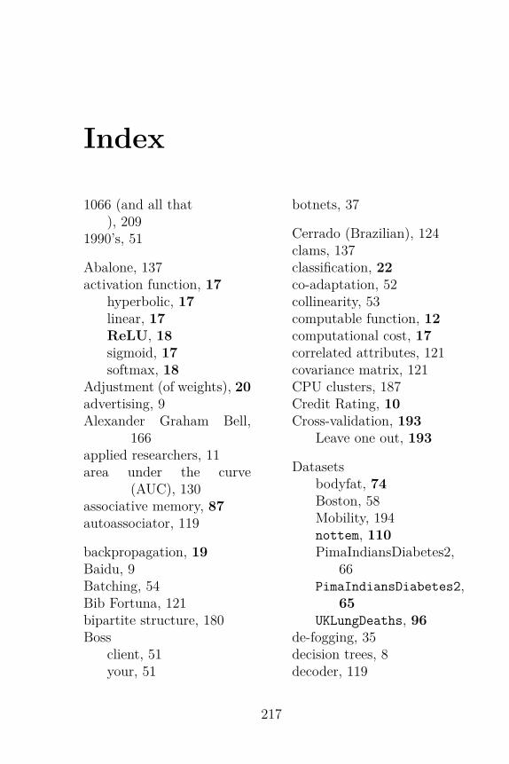
Index
1066 (and all that), 209
1990’s, 51
Abalone, 137activation function, 17
hyperbolic, 17linear, 17ReLU, 18sigmoid, 17softmax, 18
Adjustment (of weights), 20advertising, 9Alexander Graham Bell,
166applied researchers, 11area under the curve
(AUC), 130associative memory, 87autoassociator, 119
backpropagation, 19Baidu, 9Batching, 54Bib Fortuna, 121bipartite structure, 180Boss
client, 51your, 51
botnets, 37
Cerrado (Brazilian), 124clams, 137classification, 22co-adaptation, 52collinearity, 53computable function, 12computational cost, 17correlated attributes, 121covariance matrix, 121CPU clusters, 187Credit Rating, 10Cross-validation, 193
Leave one out, 193
Datasetsbodyfat, 74Boston, 58Mobility, 194nottem, 110PimaIndiansDiabetes2,
66PimaIndiansDiabetes2,
65UKLungDeaths, 96
de-fogging, 35decision trees, 8decoder, 119
217

Deep Learning Made Easy with R
diabetes, 67dimensionality reduction,
120distributional model, 67Dropout, 51drought of 1949, 209drunkenness, 48
eigenvectors, 121Elman Network
context layer, 88mean squared error, 90solar radiation, 88
encoder, 119energy function, 179energy-based model, 179England, 110entrepreneurs, 11epoch, 52equal error rate, 130
Facebook, 9failures, 50Fast Persistent Contrastive
Divergence, 186Feed Forward, 20feed forward, 14finger vein, 129fog, 35Fraud Detection, 11Friday, 48
generalization ability, 49Generative learning, 177George Box, 164Gibbs sampler, 183Goal
learning from data, 8Google, 9Great Drought of 75, 209
haze, 35Health Diagnostics, 10hidden layer, 12history(Inf), 3Hornik theorem, 42HTTPS connections, 2Human brain, 12hyperparmeter, 127
IBM, 9image compression, 40image processing, 9impute, 67industry, 9infrared, 129Initialization of the net-
work, 19input layer, 12install.packages, 1
Jabba (the Hutt), 121Jedi
Master, 120mind trick, 120Return of the, 121
Joint estimation, 74joint probability distribu-
tion, 183Jolliffe, 121Jordan Networks
context nodes, 107English weather, 110learning rate, 115
218

INDEX
memory, 108predict method, 116timeseries data, 110versus ARIMA models,
108
learningweak model, 52
log-likelihood, 182log-linear model, 34logistic activation function,
61loss function, 127
malicious software, 37Malware, 37Marketing campaigns, 10maximum likelihood, 67memory.limit, 3MetaMind, 11Metropolis Hastings ratio,
187Microsoft, 9Military Target Recogni-
tion, 10missing values, 67mist, 35MLP
as visualized in R, 14epoch, 20globally optimal solu-
tion, 21gradient descent, 19learning algorithm, 19learning rate, 21, 61,
102network error, 14
steps, 14threshold, 16
Mobility, 167model selection problem, 50mollusk (edible ), 137momentum parameter, 22Monday, 48Monte Carlo Markov chain,
183MRI, 10multiple imputation, 67
NA’s, 113na.omit method, 67National Park
Serra da Canastra, 125Neural Computing, 11Neural Networks
initializing, 21neuralnet, 42neurons, 12
bias, 17workings of, 16
NHK Broadcasting, 34nonlinear data, 8normalizing constant, 179Nottingham, 110
OCR, 11octopuses, 137Odyssey (Homer’s ), 164orthogonal transformation,
121output layer, 12
PackagesAMORE, 71
219

Deep Learning Made Easy with R
deepnet, 62MASS, 58Metrics, 57mlbench, 65neuralnet, 57quantmod, 95, 110RNSS, 95RSNNS, 69, 110TH.data, 74
packagesautoencoder, 139ltm, 167RcppDL, 167
Parallel Tempering, 186parametric model, 181partial derivative, 20partition function, 179patience, 51Paypal, 9PCA, 121Pelé, 183perceptron, 32Perceptron (original), 15Persistent contrastive diver-
gence, 186Phantom Menace, 122phylum Mollusca, 137Pima Indian, 65Portfolio Management, 10prediction, 22probability distribution,
179Process Modeling, 10professors, 49Propagation, 20
Qui-Gon Jinn, 122
R logo (image), 131random forests, 8random masking, 156reconstruction error, 127Replica Exchange Monte
Carlo MarkovChain, 186
Robin Hood, 110Rsda, 169
SAENET, 153salt and pepper noise, 156satellites (Terra and Aqua ),
125savanna, 124scallops, 137scientists, 11SDUMLA-HMT, 129sensitivity, 191set.seed, 2sparsity
constraint, 126parameter, 126
Specificity, 191spectral bands, 125Spectroradiometer, 125spyware, 37squid, 137Standardization
choices, 112standardize, 112Standardized Precipitation
Index, 209Statistics 101, 34
220

INDEX
stochastic sequence model-ing, 87
Stock MarketKOSPI, 94Nikkei225, 94SSE, 94TWSE, 94
stock market, 11str method, 66sum of squared errors, 61Supervised learning, 7supplementary Gibbs
chains, 186support vector machines, 8
T-14 hyperdrive, 122Tatooine, 122Texas (size of), 124Text Searching, 11the beautiful game, 183timeseries object, 111training patterns, 49transpose, 139Trojans, 37Twitter, 9Types of learning, 7
uncorrelated variables, 121Unsupervised learning, 7
variation, 48random, 48systematic, 49
Voice Recognition, 10
Watto, 122Wheels, 48
widgets, 48worms, 37
X-rays, 10
Yahoo, 9YouTube, 207
zoo class, 113
221

Deep Learning Made Easy with R
222

OTHER BOOKS YOUWILL ALSO ENJOY
Over 100 Statistical Tests at Your Fingertips!
100 Statistical Tests in R isdesigned to give you rapid ac-cess to one hundred of themost popular statistical tests.
It shows you, step by step,how to carry out these tests inthe free and popular R statis-tical package.
The book was created forthe applied researcher whoseprimary focus is on their sub-ject matter rather than math-ematical lemmas or statisticaltheory.
Step by step examples of each test are clearly described,and can be typed directly into R as printed on the page.
To accelerate your research ideas, over three hundred appli-cations of statistical tests across engineering, science, and thesocial sciences are discussed.
100 Statistical Tests in R
ORDER YOUR COPY TODAY!
223

Deep Learning Made Easy with R
AT LAST! Predictive analytic methods within easyreach with R...
This jam-packed book takesyou under the hood with stepby step instructions using thepopular and free R predictiveanalytic package.
It provides numerous ex-amples, illustrations and ex-clusive use of real data to helpyou leverage the power of pre-dictive analytics.
A book for every data an-alyst, student and applied re-searcher.
ORDERYOUR COPY TODAY!
224

INDEX
"They Laughed As TheyGave Me The Data To Analyze...But Then They SawMy Charts!"
Wish you had fresh ways topresent data, explore rela-tionships, visualize your dataand break free from mundanecharts and diagrams?
Visualizing complex rela-tionships with ease using Rbegins here.
In this book you will findinnovative ideas to unlockthe relationships in your owndata and create killer visualsto help you transform yournext presentation from goodto great.
Visualizing Complex Data Using R
ORDER YOUR COPY TODAY!
225

Deep Learning Made Easy with R
ANNOUNCING...The Fast & Easy Way to MasterNeural Networks
This rich, fascinating, acces-sible hands on guide, putsneural networks firmly intothe hands of the practitioner.It reveals how they work, andtakes you under the hoodwith an easy to follow pro-cess showing you how to buildthem faster than you imag-ined possible using the pow-erful, free R predictive ana-lytics package.
Here are some of the neu-ral network models you willbuild:
• Multi layer Perceptrons
• Probabilistic NeuralNetworks
• Generalized RegressionNeural Networks
• Recurrent Neural Net-works
Buy the book today and master neural networks the fast &easy way!
ORDER YOUR COPY TODAY!
226

INDEX
Write your notes here:
227

Deep Learning Made Easy with R
Write your notes here:
228

INDEX
Write your notes here:
229

Deep Learning Made Easy with R
Write your notes here:
230

INDEX
Write your notes here:
231

Deep Learning Made Easy with R
Write your notes here:
232

INDEX
Write your notes here:
233

Deep Learning Made Easy with R
Write your notes here:
234

INDEX
Write your notes here:
235