Lulu Tunu Kaaya of University
142
BIOLOGICAL ASSESSMENT OF TROPICAL RIVERINE SYSTEMS USING AQUATIC MACROINVERTEBRATES IN TANZANIA, EAST AFRICA. by Lulu Tunu Kaaya Thesis Presented for the Degree of Doctor of Philosophy in Zoology in the Department of Biological Sciences Faculty of Science University of Cape Town January 2014 ___________________________________________________________________________ University of Cape Town
Transcript of Lulu Tunu Kaaya of University
BIOLOGICAL ASSESSMENT OF TROPICAL RIVERINE SYSTEMS USING AQUATIC MACROINVERTEBRATES IN TANZANIA, EAST AFRICA.
by
Lulu Tunu Kaaya
Thesis Presented for the Degree of Doctor of Philosophy in Zoology
in the Department of Biological Sciences
Faculty of Science
University of Cape Town
January 2014
___________________________________________________________________________
Univers
ity of
Cap
e Tow
n
The copyright of this thesis vests in the author. No quotation from it or information derived from it is to be published without full acknowledgement of the source. The thesis is to be used for private study or non-commercial research purposes only.
Published by the University of Cape Town (UCT) in terms of the non-exclusive license granted to UCT by the author.
Univers
ity of
Cap
e Tow
n

Declaration
__________________________________________________________________________________
L.T.Kaaya, Ph.D. Thesis, UCT, 2014 i
Declaration
___________________________________________________________________________
This thesis reports original research carried out under the Department of Biological Sciences, Faculty of Science, University of Cape Town, between 2010 and 2013 for the Ph.D. study purpose. It has not been submitted in whole or in part for a degree at any other university. The data presented here are my own. I have fully acknowledged any received assistance.
L.T. Kaaya
Dedication
__________________________________________________________________________________
L.T.Kaaya, Ph.D. Thesis, UCT, 2014 ii
Dedication
With love and respect, I dedicate this thesis to
My mom, mzaa chema, Pulcheria Mwasu, for giving me the best you could; My husband, George Venance
Lugomela for love, support and encouragement; My sons, Harrison Limbu Lugomela and Ileme Emmanuel
Lugomela for love and patience with an absentee mummy; My sisters, Lili Pendo Kaaya and Noela Nuru Kaaya
for the whole sisterhood package..
Table of Contents
__________________________________________________________________________________
L.T.Kaaya, Ph.D. Thesis, UCT, 2014 iii
Table of Contents
Declaration............................................................................................................................ i
Dedication............................................................................................................................ ii
Table of Contents ................................................................................................................. iii
Acknowledgements .............................................................................................................. iv
Abstract ............................................................................................................................... v
Chapter 1: General Introduction ................................................................................................. 1
Chapter 2: Materials and Methods .............................................................................................. 9
Chapter 3: Screening and Selection of Reference sites .................................................................. 23
Chapter 4: River Types Classification ........................................................................................ 36
Chapter 5: Tanzania River Scoring System (TARISS): a Macroinvertebrate-based Biotic index for Rapid assessment of Rivers ............................................................................................................. 52
Chapter 6: Influence of Temporal variation on Bioassessment ......................................................... 75
Chapter 7: Influence of Spatial variation on TARISS Reference Conditions ......................................... 87
Chapter 8: Synthesis and General Discussion ........................................................................... 110
References ....................................................................................................................... 117
Appendices ...................................................................................................................... 129

Acknowledgements
__________________________________________________________________________________
L.T.Kaaya, Ph.D. Thesis, UCT, 2014 iv
Acknowledgements
I wish to express my sincere gratitude to all people who have contributed to the accomplishment of this work in different ways. Your presence in and being part of my life in any way during these three years has been the greatest support. I am thankful to my God for all his provision and grace.
To my husband George and our sons Harrison and Ileme, your love, patience, support and encouragement is what kept me going and focused. George, I do appreciate for everything. I specially thank Mary Deus, Esta Selungwi, Daria Hafati, Fatina Rajabu and all others who in one way or another looked after, cared for and loved my children in my absence.
I am greatful to the University of Dar es Salaam (UDSM), Tanzania, through the UDSM/World Bank scholarship, for funding my Ph.D. studies. I also express my gratitude to the Department of Aquatic Sciences and Fisheries, University of Dar es Salaam for extending the scholarhip opportunity. Without this financial support, this work would have remained a dream in my head.
Thank you a thousandfold Assoc. Prof. Jenny Day and Dr. Helen Dallas for being my mentors and supervisors. Your transparent and constructive comments and criticism from the proposal development stage to the end of the thesis has not only shaped my thesis but also my thinking as a scientist. Jenny, you have been a warm, caring and understanding mentor; Helen you have been a considerate, caring and friendly mentor. It has been a pleasure studying under your team of guidance.
Gratitudes to technical and scientific expertise: Mr. Amos Lugata at the University of Dar es Salaam for nutrient analyses, Dr. Helen-James-Barbs at the Albany National Museum, Grahamstown, South Africa, for taxonomic knowlegde and assistance’ Ms. Eudosia Materu, Dr. Radhia Ideva and Mr. Bahati Sosthenes for assisting in the field, Mr. William Lugomela, Mr. Erasto Ngongoloo, and Mr. Michael Manyaki for long and safe drives in search for river sites.
Institutional support: The Department of Aquatic Sciences and Fisheries, University of Dares Salaam for provision of laboratory space and equipments, the Pangani Basin water Office for support, the Arusha National Park for constant logistics support during fieldwork within the park (special thanks to the park ecologist, Ms. Gladys Ngumbi), Mantra Tanzania, through Mkuju River project for constant support, facilitation and hospitality during the field work in the Mkuju area (special thanks to the Environment Department team under Mr. Johnie Ntukula and the safety Department for rescues). Without support from all these institutions, this research would have been impossible.
To all my friends, thank you for encouragement and support. Lili and Noela for believing in me, Zingfa and Welly, you made me feel at ease, the chats and laughs made the survival trick. Zingfa, you have always been a true friend and have inspired me in times of stress and worries. Salome thanks for the encouragement and for being there.
Abstract
__________________________________________________________________________________
L.T.Kaaya, Ph.D. Thesis, UCT, 2014 v
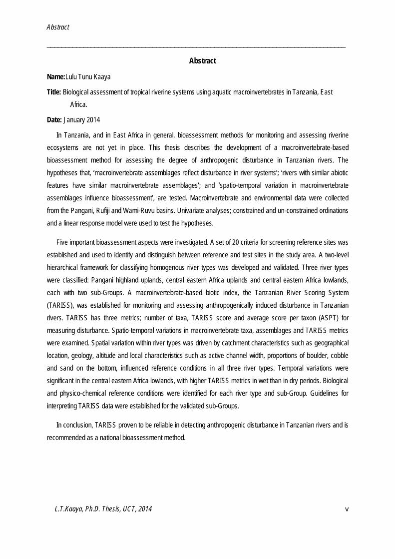
Abstract
Name:Lulu Tunu Kaaya
Title: Biological assessment of tropical riverine systems using aquatic macroinvertebrates in Tanzania, East Africa.
Date: January 2014
In Tanzania, and in East Africa in general, bioassessment methods for monitoring and assessing riverine ecosystems are not yet in place. This thesis describes the development of a macroinvertebrate-based bioassessment method for assessing the degree of anthropogenic disturbance in Tanzanian rivers. The hypotheses that, ‘macroinvertebrate assemblages reflect disturbance in river systems’; ‘rivers with similar abiotic features have similar macroinvertebrate assemblages’; and ‘spatio-temporal variation in macroinvertebrate assemblages influence bioassessment’, are tested. Macroinvertebrate and environmental data were collected from the Pangani, Rufiji and Wami-Ruvu basins. Univariate analyses; constrained and un-constrained ordinations and a linear response model were used to test the hypotheses.
Five important bioassessment aspects were investigated. A set of 20 criteria for screening reference sites was established and used to identify and distinguish between reference and test sites in the study area. A two-level hierarchical framework for classifying homogenous river types was developed and validated. Three river types were classified: Pangani highland uplands, central eastern Africa uplands and central eastern Africa lowlands, each with two sub-Groups. A macroinvertebrate-based biotic index, the Tanzanian River Scoring System (TARISS), was established for monitoring and assessing anthropogenically induced disturbance in Tanzanian rivers. TARISS has three metrics; number of taxa, TARISS score and average score per taxon (ASPT) for measuring disturbance. Spatio-temporal variations in macroinvertebrate taxa, assemblages and TARISS metrics were examined. Spatial variation within river types was driven by catchment characteristics such as geographical location, geology, altitude and local characteristics such as active channel width, proportions of boulder, cobble and sand on the bottom, influenced reference conditions in all three river types. Temporal variations were significant in the central eastern Africa lowlands, with higher TARISS metrics in wet than in dry periods. Biological and physico-chemical reference conditions were identified for each river type and sub-Group. Guidelines for interpreting TARISS data were established for the validated sub-Groups.
In conclusion, TARISS proven to be reliable in detecting anthropogenic disturbance in Tanzanian rivers and is recommended as a national bioassessment method.

__________________________________________________________________________________
L.T.Kaaya, Ph.D. Thesis, UCT, 2014 vi
Frontispiece: Pictures (a-d) show a variety of largely natural river systems in Tanzania; picture e) shows the in
situ macroinvertebrate identification process and picture f) shows a collection of macroinvertebrates from Tanzania
a
b d c
e
f)

General Introduction
__________________________________________________________________________________
L.T.Kaaya, Ph.D. Thesis, UCT, 2014 1
Chapter 1: General Introduction

General Introduction
__________________________________________________________________________________
L.T.Kaaya, Ph.D. Thesis, UCT, 2014 2
Introduction
Tropical riverine ecosystems are increasingly deteriorating as a consequence of rapidly growing human populations, land use changes, intensified agriculture, increasing urbanization and industrialization, all of which tend to compromise the natural flow regimes (Dudgeon 1992, 2000, Pringle et al. 2000, Wishart et al. 2000, Ramírez et al. 2008). Regulated flow regimes, and other resulting impacts such as increased sedimentation and pollution, contribute to the water scarcity crisis in many tropical regions. Tanzania, being a tropical country, encounters similar challenges in relation to water scarcity. Projections indicate critical water scarcity in Tanzania by the year 2050 (SWMP 2010). One of the objectives in the Ministry of Water and Irrigation (MOWI), Tanzania, is to ensure provision of water resources at acceptable quality (URT 2002). This objective is partly to be achieved through development and implementation of practical, cost-effective water quality and pollution control assessment and monitoring programmes (URT 2002). Since establishment of this policy, the MOWI has initiated physico–chemical monitoring programmes which, due to financial constrains and lack of sufficient technical capacity, have failed to deliver systematic and sufficient data to allow analysis and interpretation of water quality status and trends.
Bioassessment provides an opportunity for protection and management of water resources and can contribute to long-term sustainability and utilization. Advantages of biological over physico–chemical assessments of river systems are that biological components integrate both short-term and long-term changes in an array of environmental variables (Jacobsen et al. 2008) and are also more cost effective. Bioassessment uses biotic components (e.g. fish, macroinvertebrates, macrophytes and diatoms) and their ability to respond to environmental changes to assess the effects of human induced changes (e.g. water quality, habitat or instream flow) in riverine ecosystems (Norris and Hawkins 2000). This thesis describes a scientifically based bioassessment method of river systems which may contribute to the management and protection of water resources in Tanzania.
Bioassessment
Anthropogenic activities in and close to freshwater systems are increasing. This promotes ecosystem degradation, which in turn increases water scarcity. Anthropogenic activities have direct and indirect impacts on freshwater ecosystems. Anthropogenic activities result in domestic discharges, industrial effluents, mining discharges, agricultural runoff, impoundments and water diversions, encroachment by riparian vegetation and the introduction of alien plants and animals. Anthropogenic activities exert multiple stresses on aquatic ecosystems leading to pollution (e.g. Dudgeon et al. 2006, Smol 2009), sedimentation (e.g. Wood and Armitage 1997), channel modifications (e.g. Gregory 2006) and loss of riparian vegetation (e.g. Nilsson and Berggren 2000) resulting in changes in biotic assemblages and in many cases eventually leading to the loss of ecosystem resilience. Traditional water quality measurements, which rely on use of chemical parameters, are becoming less suitable in monitoring programmes because most human impacts occur over time and at multiple scales and the resulting physical and biological stressors are not detected by chemical monitoring (Chaves 2008). Biotic
General Introduction
__________________________________________________________________________________
L.T.Kaaya, Ph.D. Thesis, UCT, 2014 3
assemblages respond to multiple stressors and the occurrence, variation and trend in biotic assemblages reflect changes in ecosystems they inhabit. Bioassessment methods are expected to be more efficient, effective and of lower cost than chemical methods. Bioassessment methods should also be easy to use and interpret as well as scientifically reliable and robust for providing management information and supporting decision making (Lenat and Barbour 1994, Resh et al. 1995). The concepts and principles of bioassessment have been embraced in different parts of the world and effective river bioassessment methods have been developed and applied broadly. For example the assessment programmes River Invertebrate Prediction and Classification System (RIVPACS) in the United Kingdom (Wright et al. 1984, Wright 1994), the Australian River Assessment System (AusRivAs) in Australia (Simpson and Norris 2000), the Family Based Index (FBI) in North America (Hilsenhoff 1988), South African Scoring System (SASS) in South Africa (Chutter 1998, Dickens and Graham 2002), the Namibian Scoring system (NASS) in Namibia (Palmer and Taylor 2004), the Okavango Assessment System (OKAS) in Botswana (Dallas 2009) and the Zambia Invertebrate Scoring System (ZISS) in Zambia (Lowe et al. 2013).
The use of biomonitoring to assess streams and rivers is limited in tropical regions (Jacobsen et al. 2008). Several approaches on macroinvertebrate-based bioassessment of streams and rivers have been conducted in the tropical regions of Africa (e.g. Ndaruga et al. 2004 in Kenya, Kasangaki et al. 2006 in Uganda, PWBO/IUCN 2007 in Tanzania), Asia (e.g. Mustow 2002 in Thailand) and Latin America (e.g. Henne et al. 2002 in Mexico, Baptista et al. 2007 in Brazil, Jacobsen and Marin 2007 in Bolivia). The approaches however vary from simple descriptors like abundance, richness and diversity; multivariate statistical techniques (i.e. Ordination) and biotic indices adopted from other regions i.e. (Average score per Taxon (ASPT) and Biological Monitoring Working Party (BMWP) from United Kingdom (Armitage et al. 1983), FBI (Family Biotic Index) from North America (Hilsenhoff 1988), South African Scoring System (SASS) from South Africa (Dickens and Graham 2002). The biotic indices developed for non–tropical regions were modified when applied in the tropical regions. The accuracy of the adopted indices can however be improved by adjusting the macroinvertebrate taxa composition and their sensitivity levels in the tropical region of study in relation to their occurrence in an array of anthropogenic disturbances. Modification of biotic indices for use in tropical regions is usually hindered by incomplete taxonomical resolution and seldom known sensitivity levels of many tropical taxa (Jacobsen et al. 2008). This can also be considered as a setback in the general application of biomonitoring and bioassessment in most tropical countries. Few tropical countries however have attempted to develop own macroinvertebrate based biotic indices and validate the ability of the indices to distinguish between reference and test conditions. Example, West-central Mexico (Weigel et al. 2002), South-east Brazil (Silveira et al. 2005) and Bolivia (Moya et al. 2007).
Biological Indicators in River systems
Biotic components are good indicators of river system integrity because of their ability to integrate stressors from both biotic and abiotic components (Mancini 2006). Both aquatic plants and animals (e.g. fish, macroinvertebrates, macrophytes and diatoms) have been widely used as biological indicators in bioassessment methods. Several indices based on these biotic components have been established and applied worldwide (see

General Introduction
__________________________________________________________________________________
L.T.Kaaya, Ph.D. Thesis, UCT, 2014 4
review in Dallas et al. 2010). Macroinvertebrates have been widely used in bioassessment of river systems (Wright et al. 1984, Plafkin et al. 1989, Chessman 1995, Growns et al. 1995, Chutter 1998, Barbour et al. 1999) due to their ubiquitous and diverse occurrence across a range of habitats together with their wide response range to environmental stressors.
Macroinvertebrate-based bioassessment methods range from sub-organism (e.g. cell or tissue) to ecosystem-level, but community-level methods are most widely applied (Bonada et al. 2006). At the community-level, macroinvertebrates can used to assess the condition of aquatic ecosystems by use of single-metric indices e.g. use of sensitivity or functional groups metrics or biological traits (use of species’ ecological, morphological or life-history traits) and multi-metric indices such that combination of metrics that individually describes a macroinvertebrate community or predictive modeling (multivariate or multi-metric based). Often, a high degree of heterogeneity of macroinvertebrates assemblages in time and space has been a limitation in bioassessment (e.g. Dallas 2004a and b).
Spatial and temporal variability in river systems
Lotic systems are naturally spatio-temporally heterogeneous (Ward 1989) at multiple scales (Palmer and Poff 1997). Macroinvertebrate assemblages in lotic systems show spatial and temporal variability influenced by regional, catchment or local habitat variables. Frissel et al. (1986) describes a nested hierarchical relationship where some of the catchment variables constrain the local river structure (Lammert and Allan 1999). In the nested hierarchy theory, physical and biological variables on small spatial scale are influenced by variables on a larger scale (Allen and Star 1982 and O’Neill et al. 1986). Geophysical and chemical processes (Frissel et al. 1986) and biological responses (Downes et al. 1993) constrain rivers in a hierarchical manner. Several studies on heterogeneity and variability of macroinvertebrates in rivers reveal factors that best describe patterns in macroinvertebrate assemblages: geology (Richards et al. 1997), climate (Johnson et al. 2004), water temperature (Hawkins et al. 1997), hydrological and hydraulic conditions (e.g., Wright et al. 1984, Sandin 2003, Padmore 1998, Poff and Ward 1990), geomorphology characteristics such as altitude and slope (Rowntree and Wadeson 2000), biological interactions (e.g., Kohler 1992, Kohler and Willey 1997, Downes and Keough 1998) and local habitat or biotope (Dallas 2004b).
Spatial classifications which are commonly used to describe assemblage patterns of macroinvertebrates can be either physically or ecologically based. The physically based classifications describe river types or units based on physical features of rivers which are not necessarily biologically or ecologically meaningful. Example is the geomorphic and reaches type classification of Montomery and Buffington (1998) based on sediment supply and transoprt. Ecologically based classifications identify river tpes or units based on physical descriptions which also have distinctive ecological assemblages. A good example is the Padmore (1997) which describe biotope units in which both habitat and biotic or ecological factors are incorporated. River types or units based on ecological classifications are usually biologically or ecologically meaningful which provide a useful means in intergrating ecological, geomorphological and management studies (Padmore 1998).

General Introduction
__________________________________________________________________________________
L.T.Kaaya, Ph.D. Thesis, UCT, 2014 5
Macroinvertebrate taxon richness can be different among different biotopes (Pinder et al. 1987, Collier 1995, Chessman et al.1997, Kay et al. 1999). Stone and vegetation biotopes are known to support richer macroinvertebrate taxa composition (Collier 1995, Humphries 1996, Dallas 2004b, Dallas 2007a) than sandy biotopes (Quinn and Hickey 1990, Brewin et al. 1995, Dallas and Day 2007). Difference in biotope availability at a site or in a river may influence occurrence and pattern of macroinvertebrate assemblages due to biotope preferences by different macroinvertebrate taxa. For example, stoneflies (Perlidae), mayflies (Heptageniidae, Trichorythidae, Leptophlebiidae) and beetles (Psephenidae and Elmidae) show preferences to stone or hard surface biotopes while bugs (Naucoridae and Nepidae) and beetles (Scirtidae) typically live in submerged or marginal vegetation (Gerber and Gabriel 2002).
Generally riverine systems exhibit seasonal variability in discharge (McElravy et al. 1989), biotope availability i.e in depth, velocity and substrate (Armitage et al. 1995) and in water temperature (Hawkins et al. 1997). Discharge defines the wetted perimeter (i.e. macro channel width, active width and water surface width) of a stream or river system. The wetted area determines the type and availability of aquatic habitat for macroinvertebrates. Hydraulic variables define the nature of the substrate through transfer of sediments and availability of biotopes (riffles, run, and pool) in a river system (Newson and Newson 2000). Life cycles of many aquatic organisms are cued to temperature and thus variation in temperature may affect reproductive phases and development rate of macroinvertebrates (Dallas, 2004a, 2008). Because taxa differ in optimal and tolerance ranges for different physiological processes, particularly reproduction and growth, extremely high or low temperatures may contribute to extinction of intolerant taxa (Hawkins et al. 1997) or proliferation of opportunistic tolerant taxa. Seasonal availability and abundance of food may also influence life cycles of stream assemblages (Ross 1963 in Spoker et al. 2006). All of these features may result in changes in taxonomic composition of macroinvertebrate assemblages.
Hydrological seasonality is a typical feature of tropical streams and rivers and seasonality is shown by alternating wet and dry periods influencing seasonality in water depth and velocity, water chemistry and metabolic rates, dissolved and suspended solids, as well as organic matter and nutrients (Lewis 2008). In the tropics, riverine seasonality is based primarily on hydrology rather than hydrology in conjunction with temperature because tropical streams and rivers are relatively thermally stable, inferring higher and more stable metabolic rates (Lewis 2008). Seasonal variation of hydrological and hydraulic variables directly influences the occurrence and patterns of macroinvertebrate between seasons (McElrary et al. 1989, Linke et al. 1999). Different macroinvertebrate taxa show preference for the dry or the wet period. Dry periods have more stable flows in comparison to wet periods which are characterized by unpredictable intense rainfall events and spates which can have significant impacts on macroinvertebrates populations (Dudgeon 2000). There is no general pattern of seasonality in macroinvertebrate assemblages in the tropics. Studies have shown a range, varying from aseasonality patterns of Ephemeropterans composition and density in Rio Sabalo in Costa Rica (Flowers and Pringle 1995) to bimodal pattern in total macroinvertebrate abundance from the same stream in Rio Sabalo in

General Introduction
__________________________________________________________________________________
L.T.Kaaya, Ph.D. Thesis, UCT, 2014 6
Costa Rica (Ramírez and Pringle 1998) and trimodal pattern in Elmidae, Chironomidae, Trichoptera and Ephemeroptera in the Ecuadorian Andes (Turcotte and Harper 1982).
Previous studies have shown the influence of seasonality on various biotic indices for example, the taxon richness and Family Biotic Index (Link et al. 1999) and the Fraser river predictive model (Reece et al. 2001). The primary objective of bioassessment is to detect the degree of impact at a test or monitoring site; often by comparing it to a reference site or reference condition. Thus it is important to ensure the accuracy and reliability of the reference condition by understanding, reducing and eliminating potentials for seasonal variability (Dallas 2004a). Reference conditions developed for specific seasons are expected to be most reliable in assessing ecosystem changes within that particular season.
Reference Condition Approach
One form of bioassessment is the use of biotic index-based rapid protocols that utilise a reference condition approach (Barbour et al.1999, Bailey et al. 2004). In the reference condition approach, biological integrity of a test site is assessed on the basis of deviation of condition of its biological community from that found in a similar un-impacted river type (Reynoldson et al. 1997, Wright et al. 1984, Economou 2000, Wallin et al. 2003, Bailey et al. 2004). It is recognized that pristine conditions no longer exist, thus the reference condition has been referred to as the near-natural, un-impacted or least-impacted condition (Stoddard et al. 2006). The reference condition is usually defined based on information from a group of similar sites; hence it is more robust than a single reference because numerous sites function as replicates of the reference condition (Reynoldson et al.1997 and Chaves 2008). Reynoldson et al. (1997) defines a reference condition as a “representation of a group of minimally disturbed sites organized by selected physical, chemical and biological characteristics”. Reference conditions can be established by; surveys of potential reference sites, historical data, paleo-construction, modeling and expert judgment (Hughes 1995, Barbour et al. 1996 and Economou 2002). Surveying potential sites is the most direct and recommended method except for areas where potential reference sites are not available (Barbour et al. 1996, Wallin et al. 2003, Nijboer et al. 2004). Surveying of potential sites is often limited by availability of suitable and adequate potential reference sites and is expensive to achieve. Potential reference sites are identified by use of pre-defined criteria for human disturbance and further validated by either biotic or abiotic variables (Nijboer et
al. 2004). Reference conditions need to be described within homogenous regional classes or river types and referred to as-type specific reference conditions. The advantage of type-specific reference condition is that several sites occurring in the particular river type can be compared with the same reference condition.
River type classification
A river type is an ecological entity, with limited internal variation in biotic and abiotic components, which shows discontinuity with neighboring entities (Herring et al. 2003). Classification or typing of river systems is crucial in order to enable comparison of test sites to appropriate reference conditions (Dodkin et al. 2005). The aim of typing river systems is to partition the natural variability of biological conditions within a broader region by

General Introduction
__________________________________________________________________________________
L.T.Kaaya, Ph.D. Thesis, UCT, 2014 7
grouping similar un-impacted rivers based on factors such as catchment area, river size, altitude, geology or geomorphology (Economou 2002). In addition, typing simplifies planning and development of research, assessment, conservation and management of riverine ecosystems (Hawkins et al. 2000, Verdonschot and Nijboer et al. 2004, Chaves 2008). River types can be defined by either top-down approaches, which use abiotic data, or bottom-up approaches which use field-based abiotic or biotic data obtained from identified reference sites. River types obtained from the top-down approach are not necessarily biologically meaningful, although the approach is easy, fast and requires little data. The bottom-up approach requires large data sets and is time-consuming but results in a biologically meaningful classification of river types. A suitable classification of rivers is one that gives a reasonable number of river types for practical assessment and monitoring programmes; and also gives biologically meaningful river types that incorporate natural biological variability. Examples of river typing systems include the European Water Framework Directive System A which define types according to ecoregions and uses fixed categories for mandatory factors namely catchment area, distance from source and geology; and System B which does not give fixed categories for these mandatory descriptors and includes two additional obligatory variables namely, latitude and longitude; and a variety of optional physical factors (Munne and Prat 2004, Dodkins et al. 2005, Chaves 2008). In biological assessment, developing a reference condition for measuring ecosystem changes and accounting for natural variability of the biotic assemblages can be challenging. The important concept relates to the capability to differentiate between natural variability and anthropogenic effects. Partitioning a study area into relatively homogenous regions has been an approach for taking regional variability into account i.e. geographical differences (climatic, hydrological and biogeographic) (Economou 2002). Partitioning of rivers based on both regional and local characteristics produces classification groups that incorporate natural variability in macroinvertebrate reference conditions.
Derivation of TARISS (Tanzania River Scoring System) as a bioassessment index
A biotic index is a numerical expression of organism assemblage’s sensitivity or tolerance to the magnitude of disturbance in their habitat. The principle of biotic indices is that sensitive taxa disappear as the magnitude of disturbance increases and the overall number of taxa is reduced with increasing disturbance. The usefulness and robustness of biotic indices is that they pool together information on a list of taxa, technical explanations, complex interactions and disturbance responses of an aquatic community into quantitative values corresponding to quantitative ecological quality class. Biotic assemblages exhibit regional variation and because biotic indices are developed based on organism’s sensitivity or tolerance, biotic indices are normally developed for specific regions in order to account for regional variation.
SASS, the South African Scoring System is a macroinvertebrate based index developed specifically for South African rivers. The method was developed by Chutter (1998) based on the Biological Monitoring Working Party (BMWP) which was developed in United Kingdom (Armitage et al. 1983, Walley and Hawkes 1996). The method has been applied and revised in all regions of South Africa and sensitivity weightings were revised and finalized in SASS version 5 (Dickens and Graham 2002). In addition, SASS has been extensively tested in terms of its

General Introduction
__________________________________________________________________________________
L.T.Kaaya, Ph.D. Thesis, UCT, 2014 8
performance in relation to spatial, temporal and habitat variability (Dallas et al. 1995, Dallas 1997, 2004a, b). SASS is known to be a useful method in South Africa and forms the backbone of the South African national River Health programme (Uys 1996). SASS has also been modified and tested in other southern Africa countries including Namibia (Palmer and Taylor 2004), Botswana (Dallas 2009) and Zambia (Lowe et al. 2013). The degree of modification of the method differed among the countries. In Namibia modifications were on the type, number and sensitivity weightings of some macroinvertebrate families (Palmer and Taylor 2004) while in Botswana the major modifications were on the sampling protocol in terms of habitats (biotopes), sampling time and sensitivity weightings (Dallas 2009).
Currently there is no macroinvertebrate-based index for river systems in the East African region. In contrast to southern Africa, the East African region experiences a tropical climate which may result in differences in macroinvertebrate assemblage patterns in terms of taxa present and their sensitivity or tolerance to anthropogenic disturbances. Given that the bioassessment tool based on macroinvertebrates is useful in river management, the adaptation and validation of SASS for Tanzanian rivers is a priority.
Study Aim and Objectives
This study aims to develop a macroinvertebrate based bioassement tool for streams and rivers in Tanzania. To achieve this aim, several important components in bioassessment context have been addressed. The specific objectives of this study are:
Developing a procedure for identifying and screening reference sites (Chapter 3).
Develeoping a framework for river classification in Tanzania (Chapter 4)
Modifying SASS into TARISS for application in Tanzanian streams and rivers Chapter 5).
Validating TARISS using empirical data from Tanzanian streams and rivers (Chapter 5)
Assesing the robustness of TARISS across spatial and temporal variations (Chapter 6 and 7).
Developing reference conditions and interpretation guidelines for TARISS (Chapter 7).

Materials and Methods
__________________________________________________________________________________
L.T.Kaaya, Ph.D. Thesis, UCT, 2014 9
Chapter 2: Materials and Methods
________________________________________________________________
Materials and Methods
__________________________________________________________________________________
L.T.Kaaya, Ph.D. Thesis, UCT, 2014 10
Introduction
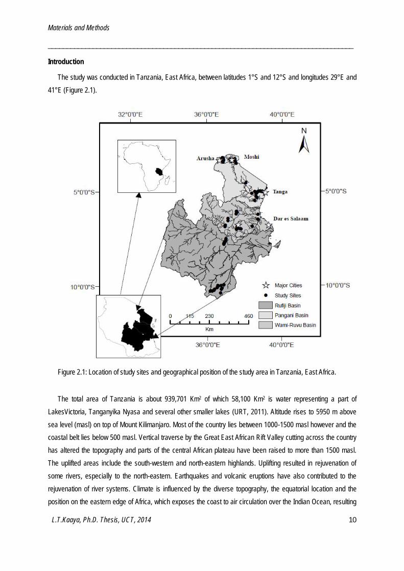
The study was conducted in Tanzania, East Africa, between latitudes 1°S and 12°S and longitudes 29°E and 41°E (Figure 2.1).
Figure 2.1: Location of study sites and geographical position of the study area in Tanzania, East Africa.
The total area of Tanzania is about 939,701 Km2 of which 58,100 Km2 is water representing a part of LakesVictoria, Tanganyika Nyasa and several other smaller lakes (URT, 2011). Altitude rises to 5950 m above sea level (masl) on top of Mount Kilimanjaro. Most of the country lies between 1000-1500 masl however and the coastal belt lies below 500 masl. Vertical traverse by the Great East African Rift Valley cutting across the country has altered the topography and parts of the central African plateau have been raised to more than 1500 masl. The uplifted areas include the south-western and north-eastern highlands. Uplifting resulted in rejuvenation of some rivers, especially to the north-eastern. Earthquakes and volcanic eruptions have also contributed to the rejuvenation of river systems. Climate is influenced by the diverse topography, the equatorial location and the position on the eastern edge of Africa, which exposes the coast to air circulation over the Indian Ocean, resulting
Materials and Methods
__________________________________________________________________________________
L.T.Kaaya, Ph.D. Thesis, UCT, 2014 11
in climatic seasonality (McClanahan 1988). The climate is classified as tropical-equatorial, ranging from hot and humid on the coast through arid lands to equatorial rain forests and cold highland areas (Griffiths 1972). Broadly Tanzania can be grouped into four climatic zones: the Lake Victoria basin, the East African highlands, the coast and the central and southern Tanzania (Ogallo 1989 and Indeje 2000). Rainfall exhibits complex transitional unimodal and bimodal patterns. Unimodal regions have a long rainy season between November and May while bimodal regions receive long rains between March and May and short rains between October and December. The short rains are more variable in time and space compared to the long rains. In many parts of the country annual rainfall varies between 200 and 1000mm while highland and mountainous regions receive up to 2000mm and the semi-arid areas receive less than 400m. Variation in mean monthly air temperature through the year are small (Griffith 1972) with mean annual temperature varying between 25oC and 32oC with hotter months being October to March and colder months from May to August. The lowest mean annual temperatures, of about 10oC, occur in the highlands and the highest, of about 35oC, occur along the coast.
Study Area
The study area is confined to the Pangani, Wami-Ruvu and Rufiji basins (Figure 2.1). The Pangani basin is characterized by Pangani and Tana ecoregions with the Pangani ecoregion occupying a larger portion of the basin while Wami-Ruvu and Rufiji basins occur in the coastal eastern Africa ecoregion. The study area gives a reasonable degree of heterogeneity among rivers and includes upland and lowland rivers, small streams and wide rivers, bedrock to alluvial systems and stone- to sandy-dominated biotopes. Further more, the study area has available and accessible least-impacted river sections that can be used to establish reference conditions. The Pangani, Wami-Ruvu and Rufiji basins provide a variety of riverine systems, climate, geology and topography with different types and levels of human disturbance. Table 2.1 gives a summary of location, climate, altitude and geological information of the Pangani, Wami-Ruvu and Rufiji basins.
Table 2.1: Location, altitude and climatic and geologic characteristics of the Pangani, Wami-Ruvu and Rufiji Basins
Pangani Wami-Ruvu Rufiji Latitude 3o03’S - 5 o 59’S 5o00’S - 7 o 00’S 5 o 35’S - 10 o 45’S Longitude 36 o 23’E - 39 o 13’E 36 o 00’E - 39 o 00’E 33o55’E - 39 o 25’E Altitude 0 – 4500 masl 0-2500 masl 0-2,960 masl Area 56,300 km2 62,024 km2 183,791 km2 Rainfall pattern Bimodal Bimodal Unimodal Annual rainfall 500-2000 mm/yr 1100-3000 mm/yr 400 – 2000 mm/yr Geology Alkaline, crystalline,
limestone, lacustrine, fluvial and estuarine
Metamorphic crystalline, metamorphic rocks and siliciclastic sediments
Schists, gneis, limestone, shells, alluvial deposits
Materials and Methods
__________________________________________________________________________________
L.T.Kaaya, Ph.D. Thesis, UCT, 2014 12
Site Selection
Preliminary site selection was undertaken by reviewing a wide range of literature including IUCN eastern Africa programme (2003), Ngoye and Machiwa (2004), EFA - Wami River Sub-Basin (2007), PWBO/IUCN (2007), PBWO/IUCN (2008) and Biervliet et al. (2009). Sites on individual rivers within the selected catchments were identified and listed together with the main activities occurring at and within 5 km of the site. Sites were selected to ensure equal distribution among the basins and their respective ecoregions.
To allow for the generation of a gradient of anthropogenic disturbance, impacted sites were selected to cover a range of disturbance types and levels. A total of 116 sites were selected as potential candidates for the study. As a result of ground-truthing of all potential sites was undertaken, during which 101 of the 116 preliminary sites were considered suitable for the study based on accessibility, safety, biotope availability and study objectives. Forty nine, 20 and 32 sites were selected from the Pangani, Wami-Ruvu and Rufiji basins respectively. Table 2.2 shows a list of the study sites and their characteristics.
Sampling procedures
Sampling was conducted both during the wet and dry periods between November 2010 and June 2012. In unimodal-rainfall regions, samples were collected during the wet (January-February) and dry (end June) periods while in bimodal regions, samples were collected in the wet periods of long (May-June) and short (November) rains and in the dry period (February). All sites were sampled in both wet and dry periods except for sites L10, L11, L12, L13 and L14 in the Rufiji basin, which were inaccessible during the rainy period. Sampling statistics were 101 sites in the dry period, 97 sites in the long rains wet period and 51 sites in the short rains wet period. Types and number of sampled biotopes in each site are given in Table 2.2. At each site macroinvertebrates, water samples and in situ physico-chemical variables were collected and measured. Additional physical characteristics related to macroinvertebrate assemblages and river ecosystem were also measured and recorded.
Benthic macroinvertebrates
Protocol for macroinvertebrate sampling was modified from the SASS method (Dickens and Graham, 2002). This is an insitu rapid bioassessment method involving identification of macroinvertebrates to family level. Macroinvertebrates are sampled using a kick-net from available stone, vegetation and gravel sand mud biotopes separately.The full description for the modified protocol including specific sampling techniques and sampling efforts is provided in Chapter 5.
Physico-chemical variables
Electrical conductivity, pH, dissolved oxygen, total dissolved solids and water temperature were measured in
situ in running waters using a multi-probe water quality meter (OAKTON® 650 LCD model) Probe measurement ranges and accuracy for each measured parameter were: pH (-2.000 to 20.000; ±0.002), conductivity (0-500 mS; ±1% full scale), total dissolved solids (0-500 ppt; ±1% full scale), dissolved oxygen (1-49.49mg/l; ±0.2mg/l) and water temperature (-10 to 110oC; ±0.5 oC).
Materials and Methods
__________________________________________________________________________________
L.T.Kaaya, Ph.D. Thesis, UCT, 2014 13
Water samples for analysis of nutrient concentrations were collected from running water, filtered in situ using 0.45 µm glass fiber filters, stored in hydrochloric-acid-washed polythene bottles and stored in a cool box at about 0-5oC and within five to six hours frozen to ≤ 10oC. In the laboratory, water samples were analyzed for soluble reactive phosphorus (PO43- -P), nitrate (NO3- -N), nitrite (NO2- -N) and ammonium nitrogen (NH4+-N) using standard spectrophotometric methods described in APHA (1995), as follows: soluble reactive phosphorus was analyzed using the molybdate-ascorbic acid method which results in a formation of intense blue colour measured at wavelength of 880nm. Ammonia was determined using a phenate method which forms a blue indophenol colour measured at wavelength of 640nm. Nitrate and nitrite nitrogen were determined using the cadmium reduction method followed by diazotisation with sulphanilamide and coupling with N-(1 naphthl)-ethylenediamine to form a highly coloured azo dye that is measured spectrophotometrically at 545nm wavelength. All spectrophotometric measurements were done using a 1 cm length glass cuvette. Linear calibration ranges were established for each nutrient parameter using calibration curves of a blank and five standards prior to analysis of samples. All water samples for nutrient analysis were analyzed within one month of collection.

Materials and Methods
__________________________________________________________________________________
L.T.Kaaya, Ph.D. Thesis, UCT 14
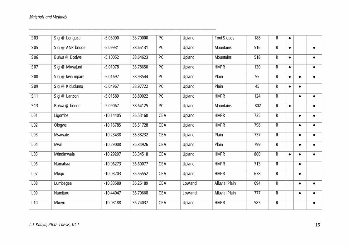
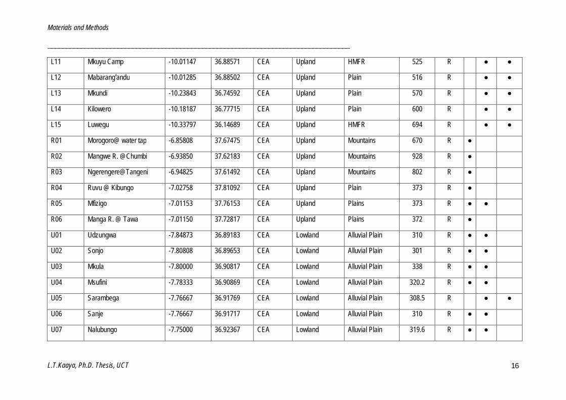
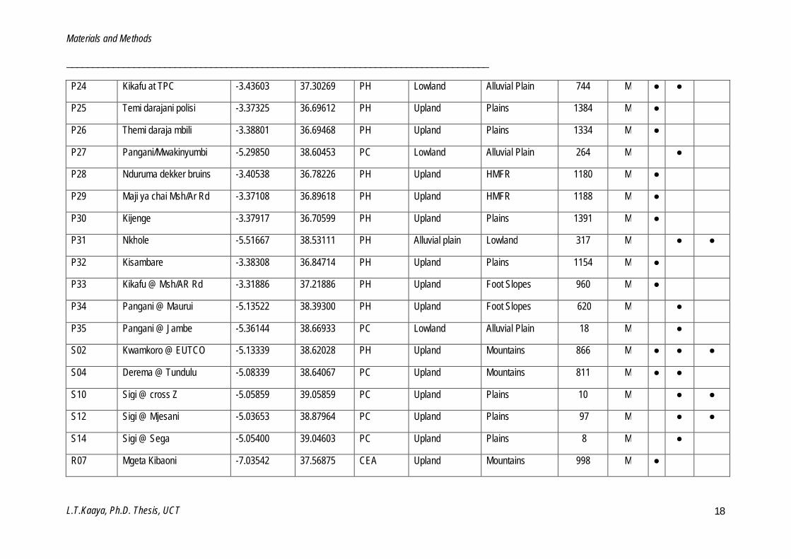
Table 2.2: List of sites investigated in this study. (Site code: (P = Pangani, S = Sigi, W = Wami, R = Ruvu, U = Udzungwa, L = Luwegu), Ecoregion: (PH = Pangani highlands, PC = Pangani coastal, CEA = Central eastern Africa, CCEA = Coastal central eastern Africa), Geomorphology: (HMFR = Hills and mountain foot ridges), Status: (R = Reference, M = Monitoring) and Biotope: (S = Stone, MV = Marginal vegetation, GSM = Gravel, sand and mud).
Site River Name Latitude Longitude Ecoregion
Geomorphologic features
Altitude Status
Biotope
Slope class Landform S MV GSM
P01 Ona @ the bridge -3.29492 37.49492 PH Upland Mountains 1469 R ● ●
P02 NAIC -3.35319 36.83653 PH Upland HMFR 1213 R ● ●
P04 Makisoro -3.29350 36.87870 PH Upland HMFR 1412 R ●
P05 Maji ya chai Darajani -3.30029 36.88180 PH Upland HMFR 1398 R ●
P06 Maji ya chai Mpakani -3.31624 36.89250 PH Upland Mountains 1336 R ●
P07 Tululusia -3.23022 36.84424 PH Upland Mountains 1607 R ●
P08 Campsite 2 -3.23299 36.84415 PH Upland Mountains 1612 R ●
P09 Tululusia/Campsite 2 -3.23004 36.84630 PH Upland Mountains 1594 R ●
P10 Maio -3.24615 36.80971 PH Upland Mountains 2155 R ●
P11 Ngarenanyuki Camp 3 -3.24521 36.84314 PH Upland Mountains 1660 R ●
P13 Magdarisho -3.35294 36.85294 PH Upland HMFR 1194 R ● ● ●
P15 Mue @ Bridge -3.30011 37.48344 PH Upland Mountains 1373 R ● ●
P17 Nduruma MSh-Ar Rd -3.37567 36.75103 PH Upland HMFR 1343 R ● ● ●
S01 Nenguruwe -5.10511 38.64529 PC Upland Mountains 561 R ●
Materials and Methods
__________________________________________________________________________________
L.T.Kaaya, Ph.D. Thesis, UCT 15
S03 Sigi @ Longuza -5.05000 38.70000 PC Upland Foot Slopes 188 R ●
S05 Sigi @ ANR bridge -5.09931 38.65131 PC Upland Mountains 516 R ● ●
S06 Bulwa @ Dodwe -5.10052 38.64623 PC Upland Mountains 518 R ● ●
S07 Sigi @ Mkwajuni -5.01078 38.78650 PC Upland HMFR 130 R ● ●
S08 Sigi @ kwa mpare -5.01697 38.93544 PC Upland Plain 55 R ● ● ●
S09 Sigi @ Kidudumo -5.04967 38.97722 PC Upland Plain 45 R ● ●
S11 Sigi @ Lanzoni -5.01589 38.80022 PC Upland HMFR 124 R ● ●
S13 Bulwa @ bridge -5.09067 38.64125 PC Upland Mountains 802 R ● ●
L01 Ligombe -10.14405 36.53160 CEA Upland HMFR 735 R ● ●
L02 Ologwe -10.16785 36.51728 CEA Upland HMFR 798 R ● ●
L03 Msawate -10.23438 36.38232 CEA Upland Plain 737 R ● ●
L04 Mwili -10.29008 36.34926 CEA Upland Plain 799 R ● ●
L05 Mtindimwale -10.29297 36.34518 CEA Upland HMFR 800 R ● ● ●
L06 Namahaa -10.06273 36.60077 CEA Upland HMFR 713 R ●
L07 Mkuju -10.03203 36.55552 CEA Upland HMFR 678 R ●
L08 Lumbegea -10.33580 36.25189 CEA Lowland Alluvial Plain 694 R ● ●
L09 Namituru -10.44047 36.70668 CEA Lowland Alluvial Plain 777 R ● ●
L10 Mkuyu -10.03188 36.74037 CEA Upland HMFR 583 R ●
Materials and Methods
__________________________________________________________________________________
L.T.Kaaya, Ph.D. Thesis, UCT 16
L11 Mkuyu Camp -10.01147 36.88571 CEA Upland HMFR 525 R ● ●
L12 Mabarang'andu -10.01285 36.88502 CEA Upland Plain 516 R ● ●
L13 Mkundi -10.23843 36.74592 CEA Upland Plain 570 R ● ●
L14 Kilowero -10.18187 36.77715 CEA Upland Plain 600 R ● ●
L15 Luwegu -10.33797 36.14689 CEA Upland HMFR 694 R ● ●
R01 Morogoro@ water tap -6.85808 37.67475 CEA Upland Mountains 670 R ●
R02 Mangwe R. @Chumbi -6.93850 37.62183 CEA Upland Mountains 928 R ●
R03 Ngerengere@Tangeni -6.94825 37.61492 CEA Upland Mountains 802 R ●
R04 Ruvu @ Kibungo -7.02758 37.81092 CEA Upland Plain 373 R ●
R05 Mfizigo -7.01153 37.76153 CEA Upland Plains 373 R ● ●
R06 Manga R. @ Tawa -7.01150 37.72817 CEA Upland Plains 372 R ●
U01 Udzungwa -7.84873 36.89183 CEA Lowland Alluvial Plain 310 R ● ●
U02 Sonjo -7.80808 36.89653 CEA Lowland Alluvial Plain 301 R ● ●
U03 Mkula -7.80000 36.90817 CEA Lowland Alluvial Plain 338 R ● ●
U04 Msufini -7.78333 36.90869 CEA Lowland Alluvial Plain 320.2 R ● ●
U05 Sarambega -7.76667 36.91769 CEA Lowland Alluvial Plain 308.5 R ● ●
U06 Sanje -7.76667 36.91717 CEA Lowland Alluvial Plain 310 R ● ●
U07 Nalubungo -7.75000 36.92367 CEA Lowland Alluvial Plain 319.6 R ● ●

Materials and Methods
__________________________________________________________________________________
L.T.Kaaya, Ph.D. Thesis, UCT 17
U08 Msolwa -7.71667 36.93536 CEA Lowland Alluvial Plain 310.4 R ● ●
U09 Sumbungulu -7.71667 36.93358 CEA Lowland Alluvial Plain 296.3 R ● ●
U10 Msowero -7.55000 37.01328 CEA Upland HMFR 318 R ● ●
W02 Mdukwe -6.10536 37.57203 CEA Upland HMFR 605 R ● ●
W03 Dikurura R. -6.10747 37.57414 CEA Upland Mountains 471 R ●
W07 Tami R. -6.47117 37.12117 CEA Upland HMFR 578 R ●
W10 Wami Matipwili -6.24250 38.71150 CCEA Lowland Alluvial Plain 20 R ●
WC01 Mzinga Kigamboni -6.51667 38.71150 CCEA Lowland Alluvial plain 18 R ● ●
P03 Themi U/S Sekei -3.35058 36.70636 PH Upland HMFR 1487 M ● ● ●
P12 Himo -3.39154 37.50415 PH Upland Foot Slopes 868 M ●
P14 Rau -3.31842 37.35175 PH Upland Foot Slopes 900 M ●
P16 Malala -3.36425 36.78300 PH Upland HMFR 1347 M ● ● ●
P18 Mbembe -3.39492 36.82825 PH Upland Plains 1134 M ● ●
P19 Kikuletwa Karangai -3.47017 36.87017 PH Upland Plains 997 M ● ●
P20 Ruvu @ Kifaru -3.52922 37.56256 PH Upland Foot Slopes 712 M ●
P21 Mkomazi R -4.57418 38.06846 PH Lowland Alluvial Plain 444 M ● ●
P22 Naura -3.37313 36.69098 PH Upland Plains 1369 M ●
P23 Luengera R -5.03208 38.54828 PH Lowland Alluvial Plain 282 M ● ●
Materials and Methods
__________________________________________________________________________________
L.T.Kaaya, Ph.D. Thesis, UCT 18
P24 Kikafu at TPC -3.43603 37.30269 PH Lowland Alluvial Plain 744 M ● ●
P25 Temi darajani polisi -3.37325 36.69612 PH Upland Plains 1384 M ●
P26 Themi daraja mbili -3.38801 36.69468 PH Upland Plains 1334 M ●
P27 Pangani/Mwakinyumbi -5.29850 38.60453 PC Lowland Alluvial Plain 264 M ●
P28 Nduruma dekker bruins -3.40538 36.78226 PH Upland HMFR 1180 M ●
P29 Maji ya chai Msh/Ar Rd -3.37108 36.89618 PH Upland HMFR 1188 M ●
P30 Kijenge -3.37917 36.70599 PH Upland Plains 1391 M ●
P31 Nkhole -5.51667 38.53111 PH Alluvial plain Lowland 317 M ● ●
P32 Kisambare -3.38308 36.84714 PH Upland Plains 1154 M ●
P33 Kikafu @ Msh/AR Rd -3.31886 37.21886 PH Upland Foot Slopes 960 M ●
P34 Pangani @ Maurui -5.13522 38.39300 PH Upland Foot Slopes 620 M ●
P35 Pangani @ Jambe -5.36144 38.66933 PC Lowland Alluvial Plain 18 M ●
S02 Kwamkoro @ EUTCO -5.13339 38.62028 PH Upland Mountains 866 M ● ● ●
S04 Derema @ Tundulu -5.08339 38.64067 PC Upland Mountains 811 M ● ●
S10 Sigi @ cross Z -5.05859 39.05859 PC Upland Plains 10 M ● ●
S12 Sigi @ Mjesani -5.03653 38.87964 PC Upland Plains 97 M ● ●
S14 Sigi @ Sega -5.05400 39.04603 PC Upland Plains 8 M ●
R07 Mgeta Kibaoni -7.03542 37.56875 CEA Upland Mountains 998 M ●

Materials and Methods
__________________________________________________________________________________
L.T.Kaaya, Ph.D. Thesis, UCT 19
R08 Ngerengere Mission -6.92264 37.60597 CEA Upland Mountains 642 M ●
R09 Kingodo -6.92264 37.60597 CEA Upland Mountains 638 M ●
R10 Mzinga Kibaoni -7.04106 37.57439 CEA Upland Mountains 1035 M ●
R11 Ngerengere @ Konga -6.91617 37.59950 CEA Lowland Alluvial Plain 531 M ●
U11 Msolwa Branch -7.71667 36.93517 CEA Lowland Alluvial Plain 307.8 M ●
U12 Kalumangala -7.76667 36.92692 CEA Lowland Alluvial Plain 301.7 M ● ●
U13 Ikela -7.70000 36.95769 CEA Lowland Alluvial Plain 290 M ● ●
U14 Muhovu -7.60000 36.99639 CEA Lowland Alluvial Plain 307 M ●
W01 Chazi R.@Magole. -6.10536 37.57203 CCEA Upland Mountains 462 M ●
W04 Diwale -6.14631 37.59631 CCEA Lowland Alluvial Plain 374 M ●
W05 Mkondoa -6.83136 36.97708 CEA Lowland Alluvial Plain 500 M ●
W06 Miyombo -6.90909 36.96622 CEA Lowland Alluvial Plain 518 M ●
W08 Mkindo -6.23569 37.55236 CEA Upland Mountains 368 M ●
W09 Kisangata R@ Mvumi -6.58783 37.12117 CEA Upland HMFR 417 M ●
WC02 Nguva at Nuta CCEA Alluvial plain Lowland 22 M ● ●

Materials and Methods
__________________________________________________________________________________
L.T.Kaaya, Ph.D. Thesis, UCT, 2014
20
Additional site characteristics
Additional information on canopy cover, channel pattern, channel type, reach type, macro channel width, active channel width, surface water width, depth average at shallow and deep biotopes and substratum composition were obtained at each site. Site conditions were also evaluated with a reflection of human disturbance using methods described in Kleynhans (1996) and Dallas (2005). Essentially information on local catchment disturbance (i.e. agriculture, urban and rural development, informal settlement, industrial development etc.), instream habitat integrity (i.e. flow modification, channel modification and bed modification) and riparian zone integrity (i.e. alien vegetation infestation, bank erosion and riparian vegetation encroachment) were recorded for use in screening and refining of potential reference sites. A field sheet for recording the river site characteristics is provided as appendix 2.1 (modified from Dallas, 2005). Detailed information on selection, screening and refining process of reference sites are given in chapter three.
Data Analysis
Univariate procedures
Univariate procedures were used to examine differences in TARISS metrics namely, number of taxa, TARISS scores and ASPT, between monitoring and reference sites (Chapter 5) and among sampling periods (Chapter 6). One–way analysis of Variance (ANOVA) was used when data were normally distributed and when data were not normally distributed an equivalent non–parametric test namely, Kruskal–Wallis was used. Assumption for normality was tested using Kolmogorov-Smirnov and Liliefurs test. The assumption of homogeneity of variances (HOV) was tested using Levene test. Not all data sets passed the HOV test, however the HOV assumption is usually not as crucial as other assumptions for ANOVA. Results in all analyses were considered significant at p < 0.005. All univariate analyses were performed using Statistica 11 software package for windows.
Multivariate procedures
Analysis of similarity (ANOSIM)
ANOSIM is a non–parametric procedure for comparing within and between class similarities to test the null hypothesis of no significant difference between groups (Clarke and Gorley 2006). One-way ANOSIM was used to test for significant differences among regional classification (Chapter 4), for replicate groups of test and reference sites (Chapter 5), for sampling periods (Chapter 6) and for selected river types (Chapter 7). ANOSIM was performed on presence/absence data, overall transformed and analysed using a Bray-Curtis similarity measure. The ANOSIM coefficient, global R, is based on the ranks of dissimilarities and ranges from -1.0 to +1.0 where R = 0 means no difference between groups and R >0 suggests differences in groups (Clarke and Gorley 2006). ANOSIM analyses were performed using PRIMER v6 software (Clarke and Gorley 2006).

Materials and Methods
__________________________________________________________________________________
L.T.Kaaya, Ph.D. Thesis, UCT, 2014
21
Canonical analysis of principal coordinates (CAP)
CAP is a constrained routine for testing differences among groups in a multivariate space by use of principal coordinates which are either best discriminating among a priori groups or have strongest correlation with particular set of variables (Anderson et al. 2008). CAP is a tool for both classification and prediction since a developed CAP model can be used to classify new points using existing points. CAP was used to build a model using taxa and their sensitivity weightings for predicting positions and sensitivity weightings of newly identified macroinvertebrate taxa (Chapter 5). CAP was also used to characterize and visualize differences between monitoring and reference sites along a continuum of human disturbance (Chapter 5) and sampling periods (Chapter 6). Canonical correlation square (δ2) of the CAP indicate the strength of the association between the multivariate data cloud and hypothesis of the group difference (Anderson et al. 2008). Canonical correspondence of principal coordinates (CAP) models were analyzed using PERMANOVA+ software package (Anderson et al. 2008), which is an add-on to PRIMER v6.
Cluster Analysis
Cluster performs simple agglomerative, hierarchical clustering to find grouping of samples such that within-group similarity is higher than between-group similarity (Clarke and Gorley 2006). Cluster analysis was performed on a Bray-Curtis resemblance matrix using group-average linking to produce dendrograms showing the clustering of samples. Cluster analysis was used to find groupings of samples within regional classifications (Chapter 4), sampling periods (Chapter 6) and within selected river types (Chapter 7). Cluster analyses were performed using PRIMER v6 software (Clarke and Gorley 2006).
Detrended correspondence analysis (DCA)
DCA estimates the degree of heterogeneity in a biological community and gives a gradient length which determines between use of either unimodal or linear response models in analyzing data from that particular biotic community (Ter Braak and Šmilauer 2002). DCA was used to determine the distribution of macroinvertebrates assemblages through calculating the gradient length and suggesting the type of response models to be used (Chapter 5). Detrended correspondence analysis (DCA) was performed using CANOCO for windows v4.5 (Ter Braak and Šmilauer 2002).
Principal component analysis (PCA)
PCA is an unconstrained ordination which projects samples in high-dimensional space onto best-fitting low-dimension space in the form of components (Clarke and Gorley 2006). The low-dimension components capture higher percentages of variability and true relationship of the original higher dimensional space and are summarized as percentage of variation. PCA was used to develop a proxy variable for the overall anthropogenic disturbance gradient across study sites (Chapter 5). PCA analyzes were performed using PRIMER v6 software (Clarke and Gorley 2006).
Materials and Methods
__________________________________________________________________________________
L.T.Kaaya, Ph.D. Thesis, UCT, 2014
22
Multi-dimensional scaling (MDS)
MDS is an unconstrained ordination which maps the number of samples in low dimensions usually two or three dimensions. The placement of samples in a map reflects the similarity and dissimilarity of biological assemblages. MDS stress values are indicators of the reliability of the relationships among the samples (Clarke and Gorley 2006). Stress values of <0.05, <0.1 and <0.2 respectively give excellent, good and useful mapping of the samples. MDS is also a complementary method to clustering, and thus interpretation may be based on both ordination and cluster analysis (Clarke and Gorley 2006). Ordination with stress values >0.2 should be used cautiously to minimize and avoid misinterpretation. Reliability of MDS ordinations were assessed by 2-dimensional stress values. MDS was used to visualize macroinvertebrate patterns within regional classifications (Chapter 4), replicate groups of monitoring and reference sites (Chapter 5), sampling periods (Chapter 6) and selected river types (Chapter 7). MDS ordinations were performed using PRIMER v6 software (Clarke and Gorley 2006).
Criteria for Screening and Selection of Reference sites
__________________________________________________________________________________
L.T.Kaaya, Ph.D. Thesis, UCT, 2014
23
Chapter 3: Criteria for Screening and Selection of Reference sites
___________________________________________________________________________

Criteria for Screening and Selection of Reference sites
__________________________________________________________________________________
L.T.Kaaya, Ph.D. Thesis, UCT, 2014
24
Introduction
Identification and screening of appropriate reference sites is an important aspect in biological assessment methods which use a reference condition approach. It is considered a critical step in establishing reference conditions (Reynoldson et al. 1997, Bailey et al. 2004, Stoddard et al. 2006, Hawkins et al. 2010) as these reference sites form the base for collecting data for establishment of reference conditions (Reynoldson et al. 1997 and Bailey et al. 2004). Reference sites are not always easily differentiated from disturbed sites and that is why the degree of impairment must be measured at each site and thus the use of a priori criteria is considered a better tool for screening of reference sites than expert judgment (Sa´nchez-Montoya et al. 2009). Human disturbance may be quantified by using biological and physico-chemical criteria. Stoddard et al. 2006 recommended that when selecting sites for biological assessment, independent criteria which do not include biotic data should be used so as to avoid circularity and preconception of the biotic structure and composition in a reference site (Bailey et al. 2004). Economou (2002) suggested that if a biological variable is used as criteria then it should not be used to determine ecological status.
Screening of reference sites has commonly been through a screening process using a pre-determined set of criteria (Hughes 1995, Barbour et al. 1996, Stoddard et al. 2006, Chaves et al. 2006, Sa´nchez-Montoya et al 2009, Hawkins et al. 2010). Screening criteria are based on different stressors that are generated by human activities that have an effect on ecological integrity, and that are capable of distinguishing a disturbed site from a reference condition (Hering et al. 2003). The goal is to obtain reference sites which fulfill the screening criteria and define a reference or acceptably healthy ecosystem (Bailey et al. 2004). Some disturbances may pass through the selection process however and it is important to further refine and validate the selected reference sites (Barbour et al. 1996). A review of studies on methods for selecting reference sites for rivers using pre-determined criteria (Barbour et al. 1996, Hughes 1995, Nijboer et al 2004, Chaves et al. 2006, 2008, Sa´nchez-Montoya et al. 2009) suggests four groups of relevant criteria: channel morphology, hydrological conditions, pollution sources and riparian vegetation. Screening criteria must allow detection of upland, riparian and instream disturbances and must be capable of recognising a disturbance even in least-stressed areas (Stoddard et al. 2006). Screening criteria give an option for the spatial scale at which screening can be done when examining reference sites. Site-specific spatial criteria are desirable (Economou 2002) as they take into account localized anthropogenic impacts such as livestock trampling, dredging, local construction, which can have significant effects on ecosystem integrity. Site-specific spatial methods are also capable of distinguishing between localized disturbance and natural variation during field visits (Wang et al. 2008).
The main objectives of this chapter are to 1) propose a set of criteria for selecting and classifying sites based on human disturbance and 2) screen and refine reference sites using site-specific criteria
Criteria for Screening and Selection of Reference sites
__________________________________________________________________________________
L.T.Kaaya, Ph.D. Thesis, UCT, 2014
25
Methods
Prior to screening and selecting reference sites, this chapter aimed at identifying most local, conspicuous and relevant criteria in the study area that can be used in the screening and selection procedure. This necessitated the use of the established set of twenty criteria as the first screening level for sites in this study. Already established methods for assessing instream and habitat integrity (Kleynhans 1996) were further used as a second step in refining the previous screening process. The refining process will also assess and indicate on the validity and performance of the established twenty criteria set in Tanzanian river catchments.
Criteria for screening reference sites
A set of twenty criteria was selected for screening reference sites. The selected screening criteria can be grouped into four broad categories, namely channel modifications, hydrological modifications, loss of riparian vegetation and water quality impairment. The screening criteria included commonly occurring land uses and ecosystem stressors effecting river ecosystems in the region. Potential sites were screened for impact by anthropogenic disturbance at a local catchment scale using the selected screening criteria. Screening criteria were rated for their anthropogenic impact at a site on a scale of 0 to 4 where, 0 = none (none in vicinity of site, no discernible impact) 1 = limited (observed in few localities with minimal impact), 2 = moderate (stress generally present with noticeable impact), 3 = (stress widespread, impact significant, small areas unaffected) and 4 = entire (stress 100% in area, impact significant). Rated screening criteria were used to calculate a local catchment human disturbance score (LCHDS). LCHDS is an index developed for quantification of the degree of anthropogenic disturbance using screening criteria in river sites of this study. LCHDS was calculated at three different spatial scales: within the riparian zone, beyond the riparian area (up to 50 m) and within 500 m upstream of the site. LCHDS calculated in each of the spatial scale was calculated by summing all rated screening criteria at a site and divided by the possible highest score (score = 80); the score is then expressed in percentage. The highest score of the three spatial scales was considered as the overall disturbance score at a site. LCHDS classified sites into five groups based on their degree of disturbance expressed as percentag: 0 - 5%, >5 – 10%, >10 – 15%, >15 – 20% and >20%. The first and second classes were considered to be reference sites, with these sites having ≥ 90% degree of “naturalness”. All sites with less than 90% naturalness were considered to be test sites.
Criteria for refining reference sites
Sites which passed the screening process were further refined using instream and riparian-zone habitat indices. This process aimed at excluding sites that were selected by the LCHDS but had instream and riparian habitat indicating certain stress levels. Instream habitat integrity (IHI) and riparian zone habitat integrity (RZHI) described by Kleynhans (1996) were used and sites with a IHI and RZHI ≥80% were selected as reference sites. This threshold score implies that the site is natural or largely natural with few modifications resulting in minimal changes in natural habitats and biota and with the assumption that ecosystem functioning is essentially
Criteria for Screening and Selection of Reference sites
__________________________________________________________________________________
L.T.Kaaya, Ph.D. Thesis, UCT, 2014
26
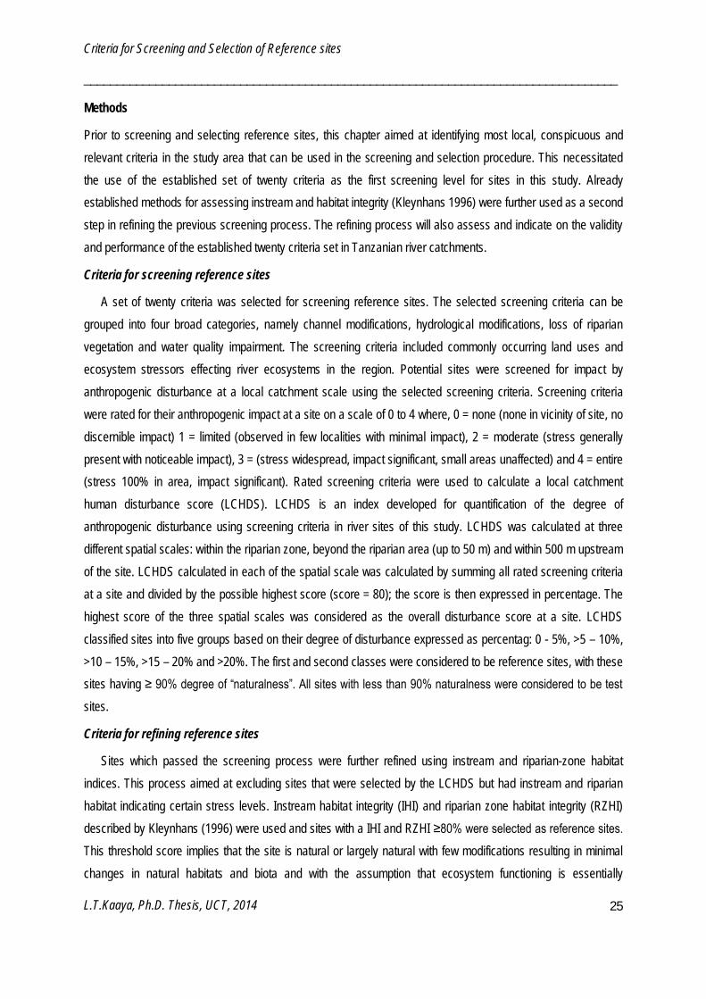
unchanged (Kleyhans, 1996). The weightings and ratings of the impacts are shown in Table 3.1 and 3.2. The total impact score is a result of the assigned impact score multiplied by the weight of the impact divided by the maximum possible impact score (25). The calculated total impacts of all criteria are then summed and expressed as a percentage and subtracted from 100 to give an instream habitat integrity score.
Table 3.1: Weighted criteria for instream habitat integrity and riparian zone habitat integrity (Kleynhans 1996) Instream Habitat Integrity Weight Riparian zone habitat integrity Weight
Bed modification 13 Channel modification 13 Channel modification 12 Change of extent of inundation 10 Change of extent of inundation 11 Flow modification 12 Flow modification 12 Presence of exotic macrophytes 9 Presence of exotic fauna 8 Solid waste disposal 6 Water abstraction 14 Water abstraction 13 Change in water quality 14 Change in water quality 13 Bank erosion 14 Exotic vegetation 12 Vegetation decrease 13
Table 3.2: Scoring system for Index of habitat integrity and riparian vegetation integrity as described in Kleynhans, 1999.
Impact Class Description Score
None No discernible impact or the modification is located in such a way that it has no impact on habitat quality, diversity, size and variability.
0
Small The modification is limited to very few localities and the impact on habitat quality, diversity, size and variability is limited.
1 - 5
Moderate The modifications are present at a small number of localities and the impact on habitat quality, diversity, size and variability are fairly limited.
6 - 10
Large The modification is generally present with a clearly detrimental impact on habitat quality, diversity, size and variability. Large areas are, however, not affected.
11 - 15
Serious The modification is frequently present and the habitat quality, diversity, size and variability in almost the whole of the defined area are affected. Only small areas are not influenced.
16 - 20
Critical The modification is present overall with a high intensity. The habitat quality, diversity, size and variability in almost the whole of the defined section are influenced detrimentally.
21- 25
Criteria for Screening and Selection of Reference sites
__________________________________________________________________________________
L.T.Kaaya, Ph.D. Thesis, UCT, 2014
27
Results
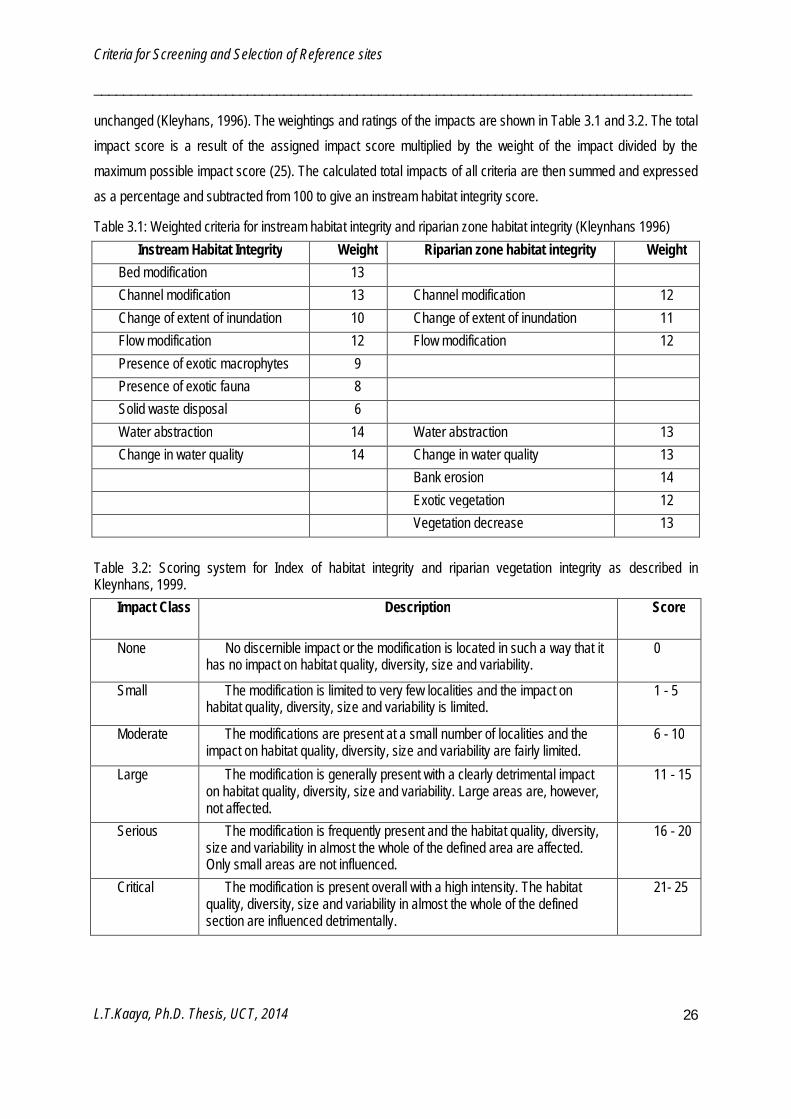
Selection criteria
A review of criteria used to select reference sites in other studies show that channel modifications, hydrological conditions, destruction of riparian vegetation and pollution source (diffuse and point source) are relevant selection criteria and were used in this study. With the background knowledge used in other regions and consideration of local conditions in the study area, twenty criteria were proposed. A list of selected criteria is shown in Table 3.3.
Table 3.3: List of selection criteria used to develop local catchment human disturbance scores (LCDHS) for screening reference sites
Criteria group Criteria (land use/ecosystem stressor) Channel modifications 1 Construction (mainly roads and bridges)
2 Livestock/wildlife disturbance (trampling) 3 Mining (sand and gravel extraction, mineral mining)
Hydrological modifications 4 Impoundments (water supply, electricity and irrigation) 5 Irrigation at small scale 6 Water abstraction (presence of pumps and pipes)
Destruction of riparian vegetation 7 Allien vegetation 8 Commercial afforestation 9 Large scale agriculture (large plantations) 10 Small scale agriculture for food crops
Diffuse and point sources pollution 11 Direct domestic activities (bathing, car washing) 12 Direct sewage disposal 13 Dumping/littering of solid wastes 14 Industrial development 15 Informal settlement 16 Roads 17 Rural development 18 Urban development 19 Water treatment plants 20 Wildlife disturbance /Livestock

Criteria for Screening and Selection of Reference sites
__________________________________________________________________________________
L.T.Kaaya, Ph.D. Thesis, UCT, 2014
28
Frequencies of occurrence of ecosystem stressors among sites
Frequencies of occurrence of each stressor among all study sites were calculated by counting sites at which a particular criterion occurred and divided by the total number of sites. The occurrence of the criteria at a particular site was analysed on the presence or absence basis. Frequencies of occurrence were calculated and expressed as percentages within the riparian zone, beyond the riparian area (up to 50 m) and within 500 m upstream the site. The frequencies were highest for dumping of solid wastes, informal settlement, small scale agriculture, direct domestic activities and alien vegetation (Figure 3.1).
0 20 40 60 80 100 120 140 160
Wildlife disturbanceWater Treatment Plants
Water abstractionUrban Development
Small Scale AgricultureRural Development
RoadsMining activities
LivestockLarge scale Agriculture
Irrigation AgricultureInformal settlement
Industrial DevelopmentImpoundment
Dumping/ LitteringDirect Sewage disposal
Direct Domestic ActivitiesConstruction
Alien vegetationAfforestation
Frequency of occurence
On site (50m) Within riparian On site (50m) Beyond riparian Upstream site (500m)
Figure 3.1: Frequency of occurrence of selected ecosystem stressors affecting the study sites as measured within the riparian zone, beyond the riparian area (up to 50 m) and within 500 m upstream of a site.
Frequencies of occurrence of stressors varied amongst the spatial scales. Within the riparian zone, higher frequencies of occurrence were obtained for dumping (46%), direct domestic services (41%), alien vegetation (38%), informal settlement (34%) and small scale agriculture (33%). Beyond the riparian zone, informal settlement (49%), dumping (46%), alien vegetation (40%), small scale agriculture (33%) and rural development (31%) had higher occurrences. Upstream of the site, highest occurrences were in direct domestic activities (44%), dumping (44%), informal settlement (39%) and small scale-agriculture (34%). Rural development and informal settlements showed increase in frequency from within to beyond the riparian zone.

Criteria for Screening and Selection of Reference sites
__________________________________________________________________________________
L.T.Kaaya, Ph.D. Thesis, UCT, 2014
29
Screening of sites
The screening process resulted in potential sixty-seven reference sites and thirty-four test sites. Thirty-two sites and thirty-five sites were included in 0–5% and >5 – 10% LCHDS categories. Eleven sites fell into LCHDS category >10 – 15% nine into the LCHDS category >15 – 20% and fourteen into the LCHDS category >20%.
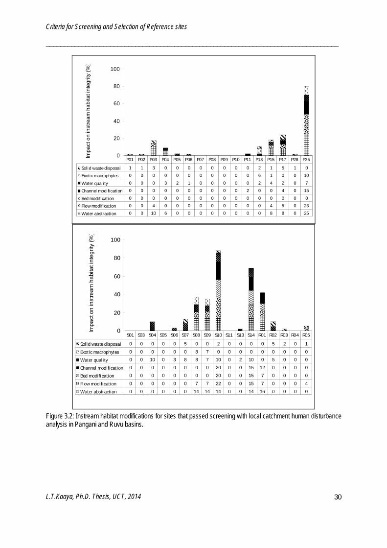
Refining of sites
Sixty-seven potential reference sites were further screened using IHI and RZHI (Figure 3.2 - 3.5). Poor water quality and solid waste disposal prevented certain sites from being reference sites. Frequency of occurrence of IHI refining criteria among the 67 sites were water quality (52%), solid waste disposal (40%), water abstraction (24%), flow modification (21%), exotic macrophytes (19%), channel modification (16%) and bed modification (6%). IHI resulted in sixty-two potential reference sites and five test sites. Sites which passed the IHI refining were further refined by the RZHI. Frequency of occurrence of RZHI refining criteria were vegetation decrease (59%), exotic vegetation encroachment (52%), water quality (51%), bank erosion (41%), flow modification (20%), water abstraction (18%) and channel modification (10%). RZHI resulted in fifty-eight reference sites and four test sites. In the end both screening and refining processes resulted in fifty eight reference and forty three test sites. Reference sites have LCHDS ≤ 10%, IHIS ≥ 80% and RZHIS ≥ 80%.
Criteria for Screening and Selection of Reference sites
__________________________________________________________________________________
L.T.Kaaya, Ph.D. Thesis, UCT, 2014
30
0
20
40
60
80
100
Impa
ct o
n in
stre
am h
abita
t int
egrit
y (%
)
Solid waste disposal 1 1 3 0 0 0 0 0 0 0 0 2 1 5 1 0
Exotic macrophytes 0 0 0 0 0 0 0 0 0 0 0 6 1 0 0 10
Water quality 0 0 0 3 2 1 0 0 0 0 0 2 4 2 0 7
Channel modification 0 0 0 0 0 0 0 0 0 0 2 0 0 4 0 15
Bed modification 0 0 0 0 0 0 0 0 0 0 0 0 0 0 0 0
Flow modification 0 0 4 0 0 0 0 0 0 0 0 0 4 5 0 23
Water abstraction 0 0 10 6 0 0 0 0 0 0 0 0 8 8 0 25
P01 P02 P03 P04 P05 P06 P07 P08 P09 P10 P11 P13 P15 P17 P28 P35
0
20
40
60
80
100
Impa
ct o
n in
stre
am h
abita
t int
egrit
y (%
)
Sol id waste disposal 0 0 0 0 0 5 0 0 2 0 0 0 0 5 2 0 1
Exotic macrophytes 0 0 0 0 0 0 8 7 0 0 0 0 0 0 0 0 0
Water qual ity 0 0 10 0 3 8 8 7 10 0 2 10 0 5 0 0 0
Channel modification 0 0 0 0 0 0 0 0 20 0 0 15 12 0 0 0 0
Bed modification 0 0 0 0 0 0 0 0 20 0 0 15 7 0 0 0 0
Flow modification 0 0 0 0 0 0 7 7 22 0 0 15 7 0 0 0 4
Water abstraction 0 0 0 0 0 0 14 14 14 0 0 14 16 0 0 0 0
S01 S03 S04 S05 S06 S07 S08 S09 S10 S11 S13 S14 R01 R02 R03 R04 R05
Figure 3.2: Instream habitat modifications for sites that passed screening with local catchment human disturbance analysis in Pangani and Ruvu basins.

Criteria for Screening and Selection of Reference sites
__________________________________________________________________________________
L.T.Kaaya, Ph.D. Thesis, UCT, 2014
31
0
20
40
60
80
100Im
pact
on
inst
ream
hab
itat i
nteg
rity
(%)
Solid waste disposal 0 2 0 1 1 0 2 2 2 2 2 3 2 1 0 1
Exotic macrophytes 0 0 0 0 0 0 0 0 1 0 0 0 0 0 0 0
Water quality 0 3 1 2 10 5 5 0 1 0 0 5 0 0 0 2
Channel modification 0 0 0 0 0 0 2 0 0 0 0 0 0 0 5 0
Bed modification 0 0 0 0 0 0 0 0 0 0 0 0 0 0 0 0
Flow modification 4 0 0 0 0 0 0 0 0 0 0 0 0 0 5 0
Water abstraction 0 0 0 0 0 0 2 0 0 0 0 0 8 0 9 0
R06 W01 W02 W03 W07 W10 WC01
U01 U02 U03 U04 U05 U06 U07 U08 U09
0
20
40
60
80
100
Impa
ct o
n in
stre
am h
abita
t int
egrit
y (%
)
Solid waste disposal 2 2 0 8 0 0 0 0 0 0 1 0 0 0 0 0 0
Exotic macrophytes 0 0 0 8 0 5 2 10 5 0 0 5 5 0 0 0 0
Water quality 5 0 0 8 0 5 5 15 15 10 0 5 5 0 0 0 10
Channel modification 0 10 5 10 0 0 0 0 0 0 0 0 0 0 0 0 0
Bed modification 0 0 1 0 0 0 0 0 0 0 0 0 0 0 0 0 0
Flow modification 0 8 0 10 0 0 0 0 0 0 0 0 0 0 0 0 0
Water abstraction 8 10 0 0 0 0 0 0 0 0 6 0 0 0 0 0 0
U10 U11 L01 L02 L03 L04 L05 L06 L07 L08 L09 L10 L11 L12 L13 L14 L15
Figure 3.3: Instream habitat modifications for sites that passed screening with local catchment human disturbance analysis in Wami and Rufiji basins.
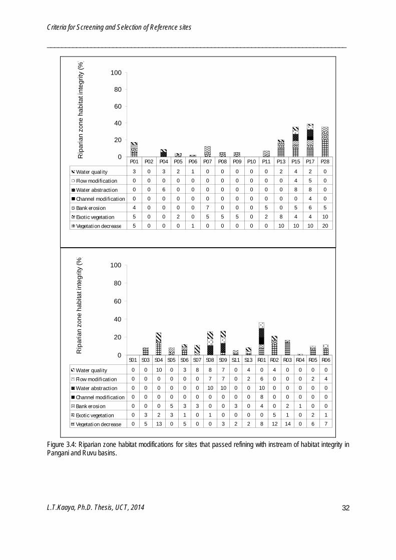
Criteria for Screening and Selection of Reference sites
__________________________________________________________________________________
L.T.Kaaya, Ph.D. Thesis, UCT, 2014
32
0
20
40
60
80
100R
ipar
ian
zone
hab
itat i
nteg
rity
(%)
Water qual ity 3 0 3 2 1 0 0 0 0 0 2 4 2 0
Flow modification 0 0 0 0 0 0 0 0 0 0 0 4 5 0
Water abstraction 0 0 6 0 0 0 0 0 0 0 0 8 8 0
Channel modification 0 0 0 0 0 0 0 0 0 0 0 0 4 0
Bank erosion 4 0 0 0 0 7 0 0 0 5 0 5 6 5
Exotic vegetation 5 0 0 2 0 5 5 5 0 2 8 4 4 10
Vegetation decrease 5 0 0 0 1 0 0 0 0 0 10 10 10 20
P01 P02 P04 P05 P06 P07 P08 P09 P10 P11 P13 P15 P17 P28
0
20
40
60
80
100
Rip
aria
n zo
ne h
abita
t int
egrit
y (%
)
Water quality 0 0 10 0 3 8 8 7 0 4 0 4 0 0 0 0
Flow modification 0 0 0 0 0 0 7 7 0 2 6 0 0 0 2 4
Water abstraction 0 0 0 0 0 0 10 10 0 0 10 0 0 0 0 0
Channel modification 0 0 0 0 0 0 0 0 0 0 8 0 0 0 0 0
Bank erosion 0 0 0 5 3 3 0 0 3 0 4 0 2 1 0 0
Exotic vegetation 0 3 2 3 1 0 1 0 0 0 0 5 1 0 2 1
Vegetation decrease 0 5 13 0 5 0 0 3 2 2 8 12 14 0 6 7
S01 S03 S04 S05 S06 S07 S08 S09 S11 S13 R01 R02 R03 R04 R05 R06
Figure 3.4: Riparian zone habitat modifications for sites that passed refining with instream of habitat integrity in Pangani and Ruvu basins.
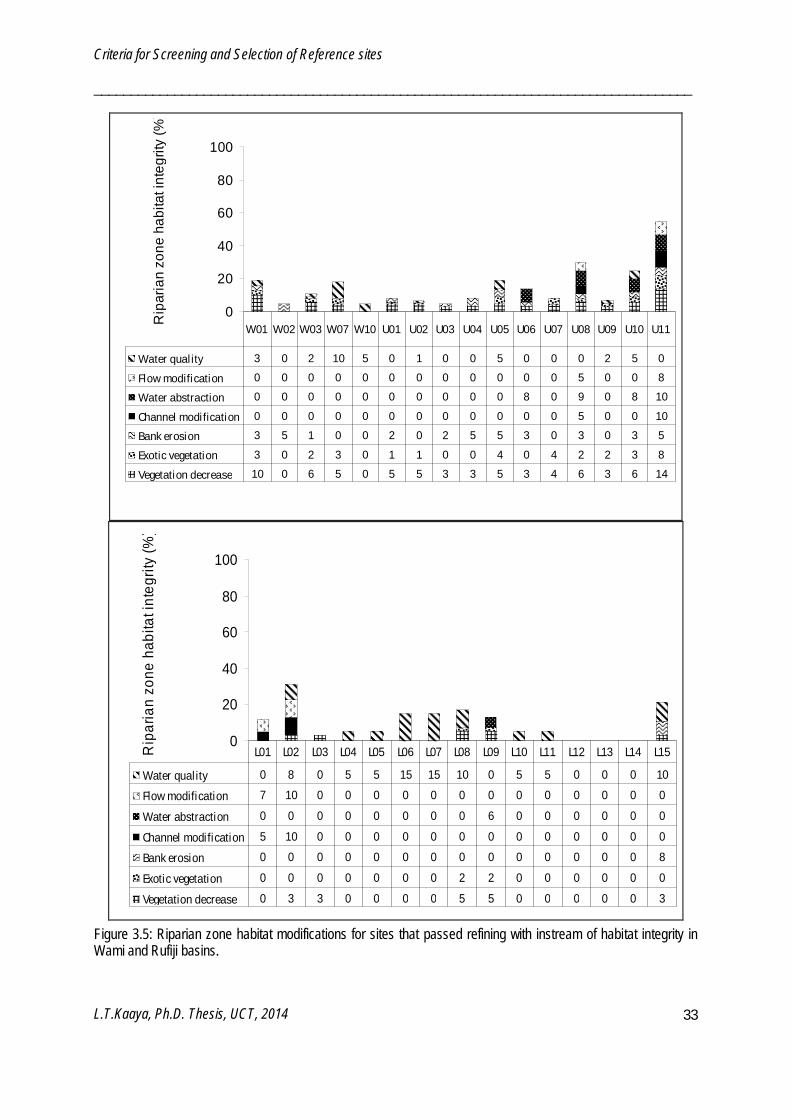
Criteria for Screening and Selection of Reference sites
__________________________________________________________________________________
L.T.Kaaya, Ph.D. Thesis, UCT, 2014
33
0
20
40
60
80
100R
ipar
ian
zone
hab
itat i
nteg
rity
(%)
Water quality 3 0 2 10 5 0 1 0 0 5 0 0 0 2 5 0
Flow modification 0 0 0 0 0 0 0 0 0 0 0 0 5 0 0 8
Water abstraction 0 0 0 0 0 0 0 0 0 0 8 0 9 0 8 10
Channel modification 0 0 0 0 0 0 0 0 0 0 0 0 5 0 0 10
Bank erosion 3 5 1 0 0 2 0 2 5 5 3 0 3 0 3 5
Exotic vegetation 3 0 2 3 0 1 1 0 0 4 0 4 2 2 3 8
Vegetation decrease 10 0 6 5 0 5 5 3 3 5 3 4 6 3 6 14
W01 W02 W03 W07 W10 U01 U02 U03 U04 U05 U06 U07 U08 U09 U10 U11
0
20
40
60
80
100
Rip
aria
n zo
ne h
abita
t int
egrit
y (%
)
Water quality 0 8 0 5 5 15 15 10 0 5 5 0 0 0 10
Flow modification 7 10 0 0 0 0 0 0 0 0 0 0 0 0 0
Water abstraction 0 0 0 0 0 0 0 0 6 0 0 0 0 0 0
Channel modification 5 10 0 0 0 0 0 0 0 0 0 0 0 0 0
Bank erosion 0 0 0 0 0 0 0 0 0 0 0 0 0 0 8
Exotic vegetation 0 0 0 0 0 0 0 2 2 0 0 0 0 0 0
Vegetation decrease 0 3 3 0 0 0 0 5 5 0 0 0 0 0 3
L01 L02 L03 L04 L05 L06 L07 L08 L09 L10 L11 L12 L13 L14 L15
Figure 3.5: Riparian zone habitat modifications for sites that passed refining with instream of habitat integrity in Wami and Rufiji basins.
Criteria for Screening and Selection of Reference sites
__________________________________________________________________________________
L.T.Kaaya, Ph.D. Thesis, UCT, 2014
34
Discussion
The initial step of selecting reference sites is important in bioassessment because evaluation of the ecosystem will be based on reference conditions. Reference sites form the comparison benchmark (Barbour et al. 1996) in the evaluation process, and must therefore be selected carefully. The criteria approach for identifying reference sites has been applied in several studies (Hughes 1995, Barbour et al. 1996, Dallas 2005, Stoddard et
al. 2006, Chaves et al. 2006, Sa´nchez-Montoya et al 2009, Hawkins et al. 2010). In this study the same approach was followed but with relevant criteria to the region under study given that the choice of criteria has an impact on the quality of reference sites. Selection criteria can vary from one region to another because of variation in landscapes and human land uses (Stoddard et al. 2006) and thus common and frequently occurring stressors were identified as screening criteria.
Extraction of boulders, gravel and sand from river beds is a common activity in Tanzania and contributes to localized modification of riverbed which may cause sediment deficiency and alter granulometric balance (Batalla 2003), which in turn affects habitat availability for biotic assemblages. Sa´nchez-Montoya et al. (2009) emphasized the importance of including sand and gravel extraction as a criterion when selecting reference sites in mediterranean rivers. Stress from wildlife through channel dredging, erosion, trampling and water quality reduction by animal wastes is also an important criterion considering the large coverage of national parks and game reserves in the country. Many rivers flow through and are a source of water in these wildlife inhabiting areas. Direct domestic activities are largely associated with poor living conditions characterise many informal settlements and unplanned rural developments. Domestic activities contribute to direct input of phosphorus, grease and oils resulting in localized eutrophic and pollution impacts. Informal settlements and unplanned rural developments in the region are also associated with dumping of solid wastes and direct sewage disposal into and within riverine ecosystems. Rivers located close to human settlements have been reported to be more polluted than rivers in agriculture and industrial areas (Ngoye and Machiwa 2004) in parts of the study area. Direct domestic activities, informal settlements and rural developments are interlinked and together increase the level of impairment and they have contributed to many sites failing to qualify as reference in this study.
Agriculture is considered in three different forms because of its varying extent, practice and potential impact on river ecosystems. Small-scale agriculture occurred at a higher frequency and had more impact than irrigation and large scale agriculture because it is the main form of economic activity for the majority of people in the country. Crops commonly grown are maize, rice and vegetables. Local farmers rarely apply good farming practices thus escalating impacts on river ecosystems such as erosion and clearance of riparian buffer zones. Most of catchment areas in Tanzania, and in particular riparian zones and associated wetland areas, have been cleared for irrigation, small-scale or large-scale agriculture. Pressure on the encroached riparian areas has facilitated colonization by alien plants. It is important and useful that these local criteria are given emphasis in selection of reference sites and their potential of localized impairment should not be underestimated.
Criteria for Screening and Selection of Reference sites
__________________________________________________________________________________
L.T.Kaaya, Ph.D. Thesis, UCT, 2014
35
The screening process led to the separation between reference and test sites. Most of the test sites did not meet pollution related criteria namely, dumping and littering, direct domestic activities and informal settlement suggesting that pollution is more significant than riparian, hydrological and channel-related criteria in the study area. The refining process was also important and validated the reference sites by excluding eleven sites which were screened as reference sites but showed certain level of instream and riparian habitat impairment. The two step process was vital to ensure the selection of only least-impaired sites as reference sites. In the refining process, loss of riparian vegetation ruled out many sites than most of hydrological and channel criteria because many riparian areas have been cleared for agricultural expansion, which is more pervasive than built-in infrastructures such as dams for hydroelectric power and municipal water supply.
The relevance of screening and refining criteria in the study area is in agreement with studies done by Hughes (1995) in United States of America, Barbour et al. (1996) in Florida, United States of America, Nijboer et al. (2004) in Europe, Chaves et al. (2006) in Portugal and Sa´nchez-Montoya et al. (2009) in Spain. All these studies agree that pollution, riparian vegetation, channel morphology and hydrological modifications are the relevant criteria in selection of reference sites but the degree of relevance of each criterion does differ. Criteria for separating reference sites from test sites in screening and refining processes were relevant to the region and capable of detecting human disturbance even at minimal levels. The criteria were operational and indicated the absence of exposure to stressors as recommended in Bailey et al. (2004). The reference sites selected can be used with confidence that whatever degree of variability they represent is a function of natural variability rather than impairment. In the next chapter, selected reference sites will be used to examine whether a priori defined river types are biologically meaningful using macroinvertebrate data.
River Types Classification
__________________________________________________________________________________
L.T.Kaaya, Ph.D. Thesis, UCT, 2014
36
Chapter 4: River Types Classification
___________________________________________________________________________

River Types Classification
__________________________________________________________________________________
L.T.Kaaya, Ph.D. Thesis, UCT, 2014
37
Introduction
Rivers are individually unique, patchy, discontinuous and strongly hierarchical systems, thus exhibiting spatial, temporal and longitudinal variability. The heterogeneity of river systems is reflected in the heterogeneous nature and distribution of fauna assemblages. Macroinvertebrate assemblages are influenced by large-scale (climate, geology, morphology) and reach-scale (hydrology, hydraulics, physico-chemical, sediment, and riparian integrity) features (Richards et al. 1997, Sandin 2003, Munne and Prat 2004, Chaves 2008). Because of these multiple and hierarchical influences at distinct spatial scales (Frissel et al. 1986, Allan et al. 1997), the hierarchical structure of rivers should be considered in bioassessment. For purposes of using macroinvertebrate assemblages in assessment and monitoring programmes, it is important that spatial, temporal and longitudinal heterogeneity are taken into account by grouping together relatively homogenous river entities. Homogenous river entities may be grouped on the basis of their similarity or differences with respect to one or more pre defined factors (Eekhout et.
al, 1997) as a classification approach which provide as spatial framework from which management approaches can be conducted (Kleynhans, et al 1998). The process of classifying rivers into homogenous river types is commonly referred to as regional classification. A river type is defined as an “artificially delineated but potentially ecological meaningful entity with limited internal biotic (taxa composition) and abiotic (physico-chemical and hydromorphological) variation and a biotic and abiotic discontinuity with an adjacent river type” (Hering et al. 2004).
Classification of rivers is a widely accepted approach in Europe (e.g. Sandin and Verdonschot 2006), United States of America (e.g. Hawkins et al. 2000), Australia (e.g. Turak and Koop 2008) and South Africa (e.g. Brown et al. 1996). Generally, classification of rivers is a useful approach in partitioning natural spatial variability (Sandin and Verdonschot 2006). There are different approaches for classifying rivers. Top-down/ regional or a priori approaches use abiotic criteria to differentiate landscape into distinct units. This is the method recommended for the European water framework directive (WFD), which uses altitude, catchment area and geology as classification criteria under the WFD system A (Munne and Prat 2004, Sa´nchez-Montoya et al. 2007). A similar regional approach has been adopted in South Africa through a hierarchical spatial framework (Dallas 2002). In this approach, a specific set of abiotic criteria are expected to be strong predictors of macroinvertebrate assemblages in a particular region. An alternative is the bottom-up approach, where biotic data collected from reference sites (Hering et al. 2004) are used to group similar river sites (Wright et al. 1984, Marchant 1997, Dodkins et al. 2005, Sa´nchez-Montoya et al. 2007). In addition, the two approaches can be combined where a
priori river types are first determined and then validated with analysis of biological data from reference sites (Gerritsen et al. 2000, Dodkin et al. 2005). Review of top-down classification systems based on landscape spatial scales (Hawkins et al. 2000) concluded that use of local habitat features leads to greater accuracy in prediction of biotic assemblages than large-scale features. Habitat structure at reach-scale is largely determined by large-scale features and upstream processes however.
River Types Classification
__________________________________________________________________________________
L.T.Kaaya, Ph.D. Thesis, UCT, 2014
38
It is therefore important to consider both large-scale and reach-scale features when classifying rivers into types.
Once river types are defined, reference conditions can be described for particular river types. Type-specific reference conditions are the basis for ecosystem evaluation and define boundaries for different classes of anthropogenic degradation. Type-specific reference conditions must be distinct from each other and within-type natural variation should not be mistaken for anthropogenic degradation (Chaves 2008). Different river types exhibit different abiotic features and biotic assemblages and even differences in their resilience to human impacts or stresses. For example, slow-flowing lowland rivers with fine bed sediments and high temperatures support different biological assemblages from those of fast-flowing mountain streams with coarse substrata and generally low water temperatures (Hering et al. 2004). The effects of channel-bed alteration (scouring, straightening and artificial bed fixation) are completely different in lowland and mountain rivers (Hering et al. 2004). Optimized river types are useful in minimizing type I error of detecting impairment when it doesn’t exist and type II error of not detecting impairment when it exist. Classifying of rivers into types has been recommended as a means of improving ecological research, conservation planning and management (Hawkins et al. 2000, Heino and Mykrä 2006).
River types have not been previously defined for Tanzania. Existing classification systems in Tanzania include the freshwater ecoregions based on fish distributional data and the ecoregion lines following hydrological boundaries (Thieme et al. 2005) and the water-basins delineation by the Department of Water Resources in the Ministry of Water and Irrigation (MOWI) Tanzania. Climatic features based on temperature and rainfall characteristics (occurrence, patterns, duration and amount) have been classified by Griffiths (1972), Ogallo (1989) and Indeje (2000) within the country and within East Africa. There is a need for integration of the above classifications and further developing a practical hierarchical spatial framework for classifying rivers in Tanzania.
This chapter’s objectives are to 1) develop a hierarchical spatial framework for classifying river types in Tanzania using abiotic factors and 2) validate the proposed classifications (river types) using macroinvertebrate data.
Materials and Methods
Delineation of river types
A literature review on river typology worldwide was conducted for a perspective on how the classification of river types can be conducted. Available local information through maps, geographic information systems (GIS), journals and reports were revised for potential relevant factors for classification of rivers in Tanzania. Reviewed topics included climate, geomorphology, topography and land use (Table 4.1). In this study a two-level hierarchical framework was used to classify river types.

River Types Classification
__________________________________________________________________________________
L.T.Kaaya, Ph.D. Thesis, UCT, 2014
39
The two-level hierarchical framework involved ‘Ecoregion classification’ as the first level and within the classified ecoregions, a second level classification; ‘Geormophology’ was used to further delineate the river systems into river types. In the first level, eight freshwater ecoregions of Africa occuring in Tanzania as described by Thieme et al. (2005) were amalgamated with five Tanzanian climatic zones described by Ogallo (1989) and Indeje (2000) to establish Tanzania freshwater ecoregions. In the second, described geological and geomorphologic by FAO (2003) were reviewed for consideration of further delineation of the level one stablished ecoregions. Geological descriprions were found to be highly varying with about 20 geological categories occurring in the country hence if used to describe river types could result in high numbers of river types which may be impractical in application. Geormophologic descriptions across the coutry had less number of categories in terms of slope classes (3) and landforms (11) thus considered to be practical. Geomorphologic descriptions are known as good physical longitudinal descriptors of riverrine systems which also have distinct biotic assemblages. As a result for the second level classification, geomorphologic features were used to further delineate the ecoregions.
Table 4.1: List of material references used in classifying river types Information Type Reference Ecoregion Book Thieme et al. (2005) Hydrology GIS Maps of Tanzania water basins Climate Book Griffiths (1972)
Journal Ogallo (1989) and Indeje (2000)
GIS Tanzania-Thematic aggregation Lithology/Landform (Food and agriculture organisation (FAO)-Africover, 2003)
Geomorphology GIS Tanzania-thematic aggregation geomorphology (FAO-Africover, 2003)
Geology GIS Tanzania-thematic aggregation geology (FAO-Africover, 2003) Land Use GIS Maps of Wami-Ruvu and Rufiji land uses
Tanzania-Land cover map (FAO-Africover, 2003)
Macroinvertebrate assemblages
Macroinvertebrates were sampled from reference sites using the TARISS (Tanzania River Scoring System) sampling protocol as described in chapter 5. Samples were collected from stone, vegetation and gravel sand mud (GSM) biotopes in the long rains, short rains and dry periods.

River Types Classification
__________________________________________________________________________________
L.T.Kaaya, Ph.D. Thesis, UCT, 2014
40
Data Analysis
Validation of regional classifications
Analysis of similarities (ANOSIM) was used to test whether or not there were significant differences in macroinvertebrate assemblages amongst classification classes of various regional classifications (Clarke and Gorley 2006). Similarities were compared separately for stone, vegetation and GSM biotopes in the long rains, short rains and dry periods. For the purpose of exploring patterns across regional classifications, sites were coded according to the river types in each regional classification. Patterns were visualized separately for wet, dry and combined wet and dry periods using by non-metric dimensional scaling (MDS) (Clarke and Gorley 2006). Classification of sites based on more than one sampling period is often recommended because it is considered to improve robustness in classifying sites as it reduces temporal variation (Turak et al. 1999).
Results
Level I: Ecoregion
Eleven freshwater ecoregions (Thieme et al. 2005) and five climatic zones (Indeje 2000) were used to develop twelve ecoregions which delineate the country based on hydrological (basin) boundaries and climatic characteristics (Table 4.2). Freshwater ecoregions of Thieme et al. (2005) were modified by clustering together freshwater ecoregions that have a common drainage point. Malagarasi-moyowosi and Lake Tanganyika, which drain into Lake Tanganyika, were combined. Small ecoregions, Bangweulu-Mweru and middle Zambezi-Luangwa, that drain into Lake Nyasa and belong to the same climatic zone, were grouped together with Lake Nyasa. The Tana ecoregion, belonging to the same climatic zone as the Pangani ecoregion, was put together with the Pangani ecoregion. Some ecoregions were divided into groups based on their climatic differences. The Lake Victoria ecoregion and the Pangani ecoregion are each characterised by three different climatic zones thus they were divided into six ecoregions: Southern Lake Victoria, Western Lake Victoria, Eastern Lake Victoria, Pangani highlands, Pangani lowlands and Pangani coastal (Table 4.2). The resulting twelve regions of Tanzania have been renamed and are referred to as ecoregions in this study.
Level II: Geomorphology
Geomorphologic descriptions and classes in FAO – Africover (2003) were used as the basis for geomorphologic delineation. Slope classes and landform features were used for the delineation. Slope classes give a broader representation of the detailed landforms. Both slope and landform classes were used as level II of classification in delineating river types. Three slope classes >0.08, 0.02 – 0.08 and <0.02 and eleven landform features namely, mountains, hills and mountain foot-ridges; escarpments; valleys; foot-slopes; structural depressions; alluvial fans; plateaux; plains; flood plains and alluvial plains; lacustrine deposits; and coastal and delta plains were used for geomorphologic classifications (Table 4.3). Geomorphologic features resulted in three slope classes and eleven landform features for classifying rivers.
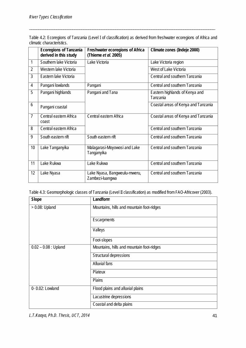
River Types Classification
__________________________________________________________________________________
L.T.Kaaya, Ph.D. Thesis, UCT, 2014
41
Table 4.2: Ecoregions of Tanzania (Level I of classification) as derived from freshwater ecoregions of Africa and climatic characteristics. Ecoregions of Tanzania
derived in this study Freshwater ecoregions of Africa (Thieme et al. 2005)
Climate zones (Indeje 2000)
1 Southern lake Victoria Lake Victoria Lake Victoria region 2 Western lake Victoria West of Lake Victoria 3 Eastern lake Victoria Central and southern Tanzania
4 Pangani lowlands Pangani Central and southern Tanzania 5 Pangani highlands Pangani and Tana Eastern highlands of Kenya and
Tanzania 6 Pangani coastal Coastal areas of Kenya and Tanzania
7 Central eastern Africa coast
Central eastern Africa Coastal areas of Kenya and Tanzania
8 Central eastern Africa Central and southern Tanzania
9 South eastern rift South eastern rift Central and southern Tanzania
10 Lake Tanganyika Malagarasi-Moyowosi and Lake Tanganyika
Central and southern Tanzania
11 Lake Rukwa Lake Rukwa Central and southern Tanzania
12 Lake Nyasa Lake Nyasa, Bangweulu-mweru, Zambezi-luangwa
Central and southern Tanzania
Table 4.3: Geomorphologic classes of Tanzania (Level II classification) as modified from FAO-Africover (2003).
Slope Landform > 0.08: Upland Mountains, hills and mountain foot-ridges
Escarpments
Valleys
Foot-slopes 0.02 – 0.08 : Upland Mountains, hills and mountain foot-ridges
Structural depressions
Alluvial fans
Plateux
Plains
0- 0.02: Lowland Flood plains and alluvial plains
Lacustrine depressions Coastal and delta plains
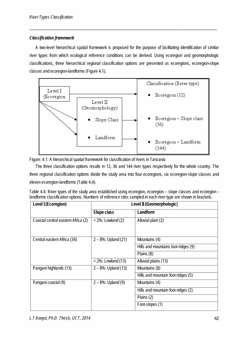
River Types Classification
__________________________________________________________________________________
L.T.Kaaya, Ph.D. Thesis, UCT, 2014
42
Classification framework
A two-level hierarchical spatial framework is proposed for the purpose of facilitating identification of similar river types from which ecological reference conditions can be derived. Using ecoregion and geomorphologic classifications, three hierarchical regional classification options are presented as ecoregions, ecoregion-slope classes and ecoregion-landforms (Figure 4.1).
Figure: 4.1: A hierarchical spatial framework for classification of rivers in Tanzania
The three classification options results in 12, 36 and 144 river types respectively for the whole country. The three regional classification options divide the study area into four ecoregions, six ecoregion-slope classes and eleven ecoregion-landforms (Table 4.4).
Table 4.4: River types of the study area established using ecoregion, ecoregion – slope classes and ecoregion - landforms classification options. Numbers of reference sites sampled in each river type are shown in brackets.
Level I (Ecoregion) Level II (Geomorphologic) Slope class Landform
Coastal central eastern Africa (2) < 2%: Lowland (2) Alluvial plain (2)
Central eastern Africa (34) 2 – 8%: Upland (21) Mountains (4) Hills and mountains foot-ridges (9) Plains (8)
< 2%: Lowland (13) Alluvial plains (13) Pangani highlands (13) 2 – 8%: Upland (13) Mountains (8)
Hills and mountain foot-ridges (5) Pangani coastal (9)
2 – 8%: Upland (9) Mountains (4) Hills and mountain foot-ridges (2) Plains (2) Foot-slopes (1)
River Types Classification
__________________________________________________________________________________
L.T.Kaaya, Ph.D. Thesis, UCT, 2014
43
The ecoregion-slope classification was selected for validating river types in this study because it gave an adequate number of reference sites with simplified geomorphologic features and produced a reasonable number of river types, which is a recommended aspect in river typology (Dodkins et al. 2005). The ecoregion-slope classification resulted in five river types: Pangani highland upland (PHU), Pangani coastal upland (PCU), central eastern Africa upland (CEAU), central eastern Africa lowland (CEAL), and coastal central eastern Africa lowland (CCEAL) for validation of regional classification. Slope values > 0.08 characterize sites in hilly and mountainous areas, which were not considered in this study because they are not easily accessible and most times are of little concern in river management because of little exposure to human disturbances. A total of 60 reference sites were used to validate regional classifications in the study area. These sites were selected using a two-step process based on disturbance levels (Chapter 3). In the validation process channel features including channel forms, bank and bed material and reach types for each site were recorded and described for their similarities and differences among the five river types.
Validation of regional classifications
Analysis of similarities (ANOSIM) was used to test for similarities of macroinvertebrate assemblages among river types obtained in each regional classification. Generally the ecoregion-landform classification showed higher significant differences than ecoregion and ecoregion-slope class classifications in both vegetation and stone biotopes.Significant differences in macroinvertebrates among river types were observed in some regional classifications, biotopes and sampling periods. Significant differences occurred in both the dry and wet periods in vegetation biotope and during the long rains and dry periods in the stone biotope.
Global R in GSM biotopes suggested no class clustering in the long rains (R=0.036, p=0.599; R=0.121, p=0.075 and R=0.352, p=0.01), dry (R=0.045, p=0.39; R=0.045, p=0.357and R=0.031, p=0.402) and short rains (R=0.188, p=0.094; R=0.188, p=0.084and R=0.27, p=0.126) in the ecoregion, ecoregion-slope class and ecoregion–landforms regional classifications. In the vegetation biotope, global R showed differences among river types with R = 0.328,p=0.008;R = 0.203 , p=0.039;and R = 0.299 , p=0.002 in the long rains, R=0.392, p=0.015; R=0.213, p=0.007 and R=0.171, p=0.026 in dry period and R=0.349, p=0.002; R=0.349, p=0.002 and R=0.419, p=0.011 in short rains in the ecoregion, ecoregion-slope class and ecoregion–landforms regional classifications. However, in vegetation data, a significant difference (p < 0.005) among river types was found in the ecoregion–landform classification in the long rains, ecoregion and ecoregion-slope class in the short rains period. Inadequate number of sites of some river types in the vegetation biotopes contributed to fewer permutations for calculation of significant differences among river types.
In the stone biotope, during the short rain period, macroinvertebrate assemblages showed significant clustering in both ecoregion (R = 0.208, p=0.001) and ecoregion–slope class (R = 0.219, p=0.001) classifications. The ecoregion–landform classification showed the clustering (R = 0.261), however not significant (p = 0.011). In long rains and dry periods global R suggested differences among all regional classification with p values < 0.005
River Types Classification
__________________________________________________________________________________
L.T.Kaaya, Ph.D. Thesis, UCT, 2014
44
signifying the differences. Stone biotope global R for each regional classification in long rains and dry periods are shown in Table 4.5. In stone biotope, global R values varied among regional classifications in each sampling period suggesting differences in classification strength among them. In both long rains and dry periods, ecoregion-landform had a higher global R (R = 0.357 and R = 0.388), followed by ecoregion (R = 0.297 and R = 0.348) and ecoregion-slope classes had lowest global R values (R = 0.144 and R = 0.269). Long rains and dry macroinvertebrate stone biotope data were combined to strengthen the classifications and this resulted in the similar trend of higher global R value in ecoregion-landforms (R = 0.362), ecoregion (R = 0.361) and least in ecoregion-slope class (R = 0.223). Pair-wise tests were done in order to identify regional classifications which showed significant differences (Table 4.5).
Patterns of macroinvertebrate assemblages in stones biotopes of wet, dry and combined long rains and dry periods were visualized using non metric multidimensional scaling in the three regional classifications (Figure 4.2 – 4.4). Stone biotope showed significant clustering across all sampling periods hence was used to visualize clustering pattterns. Macroinvertebrates patterns exhibited different spatial clustering among different river types in long rains, dry and combined wet and dry periods. In the ecoregion classification, Pangani highlands clustered separately from Pangani coastal more clearly in the dry and combined periods. In the ecoregion–slope classes, upland and lowland sites of central eastern Africa clustered separately in the dry and combined periods. In the ecoregion–landforms grouping was affected by inadequate number of sites however in combined wet and dry period, distinct groups were formed between CEAU mountains and plains, PCU mountains and plains; and CEAL alluvial plains and hills and mountain foot ridges. Pangani highland sites grouped into two, sites P07, P09, P10 and P11 and P01, P02, P13, P15 and P17.
This clustering in Pangani ecoregion was more pronounced in the dry and combined periods while in the wet period, P07 and P11 clustered separately from P09 and P10. Other sites which were repeatedly separated from the groups across sampling periods were S07, W10 and WC01 from PCU, CEAL and CCEA respectively. In the wet season, a CEAU site, R04 was separated from other sites. There was a high degree of coherence in macroinvertebrate patterns between the dry and the wet and dry combined periods. Ecoregion –landforms gave clearer patterns than the ecoregion and ecoregion–slope classes but the number of sites within each river type in the ecoregion–landforms was limited.
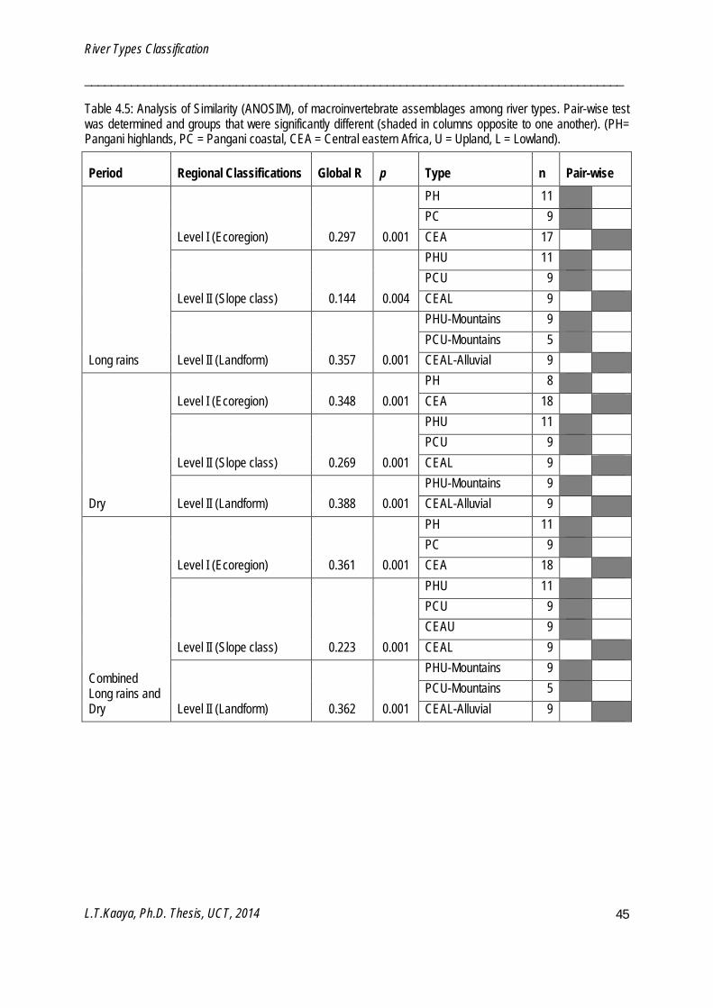
River Types Classification
__________________________________________________________________________________
L.T.Kaaya, Ph.D. Thesis, UCT, 2014
45
Table 4.5: Analysis of Similarity (ANOSIM), of macroinvertebrate assemblages among river types. Pair-wise test was determined and groups that were significantly different (shaded in columns opposite to one another). (PH= Pangani highlands, PC = Pangani coastal, CEA = Central eastern Africa, U = Upland, L = Lowland).
Period Regional Classifications Global R p Type n Pair-wise
Long rains
Level I (Ecoregion) 0.297 0.001
PH 11 PC 9 CEA 17
Level II (Slope class) 0.144 0.004
PHU 11 PCU 9 CEAL 9
Level II (Landform) 0.357 0.001
PHU-Mountains 9 PCU-Mountains 5 CEAL-Alluvial 9
Dry
Level I (Ecoregion) 0.348 0.001 PH 8 CEA 18
Level II (Slope class) 0.269 0.001
PHU 11 PCU 9 CEAL 9
Level II (Landform) 0.388 0.001 PHU-Mountains 9 CEAL-Alluvial 9
Combined Long rains and Dry
Level I (Ecoregion) 0.361 0.001
PH 11 PC 9 CEA 18
Level II (Slope class) 0.223 0.001
PHU 11 PCU 9 CEAU 9 CEAL 9
Level II (Landform) 0.362 0.001
PHU-Mountains 9 PCU-Mountains 5 CEAL-Alluvial 9
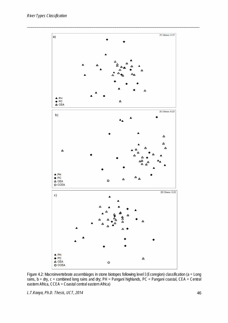
River Types Classification
__________________________________________________________________________________
L.T.Kaaya, Ph.D. Thesis, UCT, 2014
46
Figure 4.2: Macroinvertebrate assemblages in stone biotopes following level I (Ecoregion) classification (a = Long rains, b = dry, c = combined long rains and dry; PH = Pangani highlands, PC = Pangani coastal, CEA = Central eastern Africa, CCEA = Coastal central eastern Africa)
a)
... PH • PC
" CEA
b)
... PH • PC
" CEA o CCEA
c)
.. PH • PC
" CEA o CCEA
...
..
...
..
•
..
.. .. •
•
•
• o
..
•
o
20 Stress: 0_22
•
...
• • • .. •
20 Stress: 0.22
.. • ......
.. ...
.. • .. .. .. • ...
•
20 Stress: 0.22
...
• " . • • •

River Types Classification
__________________________________________________________________________________
L.T.Kaaya, Ph.D. Thesis, UCT, 2014
47
Figure 4.3: Macroinvertebrate assemblages in stone biotopes following level II (slope class) classification (a = Long rains, b = dry, c = combined long rains and dry; PH = Pangani highlands, PC = Pangani coastal, CEA = Central eastern Africa, CCEA = Coastal central eastern Africa, U = Uplands, L = Lowlands)
-
a) 20 Stress: 0 _22
• • ...
I>. ... .. I>. B 0 I>.D 0 ... ... 0 • L;. ... ... L;. O~ ~
• • • ... • .... PHU ... 0
• PCU ... • I>. CEAU L;. o CEAL
20 Stress: 0.22
b) ... • .....
• ... L;.
... I>.
L;. ....... I>. I>.
• L;. ·0 0 ... • 1>. • DO 0 ......
o 0 ... .... PHU • • ... • PCU I>. CEAU • O CEAL 0 0 01>.
o CCEAL
C) 2D Stress: 0.22
... ...
I>. ... ... • ... ... 1>.
~ CjI
'a 0
L;. I>..i:b • ... 0 L;. I>. I>. ... 0 ... I>. •
... • ... • • •
... PHU • PCU I>. CEAU 0 o CEAL 0 o CCEAL

River Types Classification
__________________________________________________________________________________
L.T.Kaaya, Ph.D. Thesis, UCT, 2014
48
Figure 4.4 (a-c): Macroinvertebrate assemblages in stone biotopes following level II (landform) classification (a = Long rains, b = dry, c = combined long rains and dry; PH = Pangani highlands, PC = Pangani coastal, CEA = Central eastern Africa, CCEA = Coastal central eastern Africa, U = Uplands, L = Lowlands).

River Types Classification
__________________________________________________________________________________
L.T.Kaaya, Ph.D. Thesis, UCT, 2014
49
Discussion
River basins are defined by differences in physical and chemical variables including climate, morphology and geology which together define riverine ecosystems and their functioning. Riverine ecosystems show spatial variation regionally and longitudinal variation along the river continuum. Such regional differences are important when considering riverine bioassessment and biomonitoring programmes. It is necessary to ensure valid comparisons by taking into account natural variability in habitat characteristics and biotic assemblages (Mykrä et
al. 2009). Classification of riverine systems into river types is one way of incorporating natural variability in habitat and biota (Reynoldson et al. 1997). River type classification is aimed at decreasing within-type variation in biotic indices and metrics so that anthropogenic changes can be determined (Dodkins et al. 2005). The importance of typing rivers and streams has been recognized worldwide. In Europe, for example, the Water Framework Directive requires each member state to classify their river systems into homogenous river types for assessment and monitoring purposes (European Commission 2000, Mykrä et al. 2009).
Ecoregions provide large-scale features which determine ecosystem structure and functioning at reach-scale (Minshall 1988) and are expected to capture geographical, climatic, latitudinal and longitudinal variation. Several studies have addressed concerns of large-scale landscape classifications such as ecoregions in accounting for variability of biotic assemblages (Hawkins et al. 2000, Sandin and Johnsons 2000, Mykrä et al 2004 and Mykrä et
al 2009) but it should be noted that large-scale features influences habitat structure (Molnar et al. 2002) and must be incorporated in the classification of rivers. In addition, biotic community variability is narrowed by use of local reach-scale features such as geomorphology. Geomorphologic processes which operate hierarchically across different scales within a riverine system (Parsons et al, 2003) controls habitat characteristics. Habitat structure and availability in riverine systems is a driver of ecological processes and responses (Orr et al. 2008) and its importance and influence on freshwater ecosystems is widely recognized (Maddock 1999, Urban and Daniels 2006). Habitat availability is one feature whereby macroinvertebrate assemblages respond to physical features at different scales (Parsons et al, 2003). Macroinvertebrates utilise specific habitat types developed by hydrological and hydraulic features such as riffles and runs. Because climatic and geomorphology features are strong predictors of macroinvertebrate assemblages (Richards et al. 1997, Hawkins et al. 2000, Chaves et al. 2005), then river types defined based on these features are considered to represent relative distinct macroinvertebrate assemblages (Sa´nchez-Montoya et al. 2007) and resulting variation represents natural variability and not impairment conditions.
This study has developed a framework for classification of rivers in Tanzania. Given the large size of the country and its varying geology, topography and climate, natural variability of biological assemblages is expected to be relatively high. Combination of hierarchical regional framework (top-down) and validation by reference biological data (bottom-up) approach was used in this study. Regional, climatic and geomorphologic features were used to develop a priori classifications.
River Types Classification
__________________________________________________________________________________
L.T.Kaaya, Ph.D. Thesis, UCT, 2014
50
Given the availability of reference sites in the study area for obtaining biological data, a posteriori classifications of macroinvertebrate assemblages were used to validate the a priori regional classifications.
Macroinvertebrate assemblages partitioned in more similarly with the a priori regional classifications. Macroinvertebrate assemblages partitioning in geomorphologic landforms had greater within–site similarity than between-site similarity compared to geomorphologic slope classes. The strength of landform over slope classes is expected, especially in the upland class (slope = 0.02 – 0.08) where plains, foot slopes, hills and mountains landforms exhibit variability in terms of their location, undulating nature and degree of steepness. In addition, upland slope classes may occur not only in the upper sections of the river but also in the lower parts of a river. This situation was encountered in the Pangani coastal, where upland hills, mountain foot ridges and plains occurred in the lower sections of the river. According to geomorphologic classification of rivers by Rowntree and Wadeson (2000), such upland areas with steep slopes occurring in the lowland sections of a river are known as rejuvenated zones and constitute characteristics of upstream rivers. Thus their biological assemblages are expected to partition separately from either upland or lowland rivers.
Among the challenges in classifying rivers is the number of river types to be produced (Dodkins et al. 2005). The number of river types has practical implications in bioassesment. Large numbers of river types may result in a complex and not easily understood typology, while low number may not effectively account for natural variability (Mykra et al. 2009). River typology should be simple, easily understood and efficiently portray variability of biotic assemblages (Heini and Mykra 2006, Mykra et al. 2009). In addition the number of river types should allow enough representation of reference sites in order to improve confidence in the definition of a reference conditions (Dodkins et al. 2005). The regional classifications in this study results in 12, 36 and 144 river types based on ecoregion, ecoregion–geomorphologic slope classes and ecoregion–geomorphologic landforms respectively. Through ANOSIM all regional classifications suggested differences in macroinvertebrate assemblages among their river types. Therefore any of the three regional classifications can be used to define river types with assurance of biologically meaningful classification. The ecoregion–geomorphologic landforms classification gives a stronger partitioning of the macroinvertebrate assemblages and may have higher power of detecting changes in biological assemblages but, because of the large number of river types it may be impractical in terms of availability of sufficient reference sites and financial resources. The ecoregion classification produces fewer river types which would unlikely represent adequately all natural variability and be capable of detecting changes in an ecosystem.
However, validation of ecoregion classification using macroinvertebrate assemblages revealed distinctions among ecoregions which support the use of ecoregion partitioning as a means of classifying rivers. The advantage of using a classification system with few river types is the availability of sufficient reference sites to produce robust reference conditions which can be applied in a broader area.
River Types Classification
__________________________________________________________________________________
L.T.Kaaya, Ph.D. Thesis, UCT, 2014
51
It should be noted that the choice of regional classification to be adopted should be determined by project objectives, financial resources and long–term water resources management goals.
In conclusion, ordination analysis and ANOSIM suggest that macroinvertebrate assemblages correspond to regional classifications despite that there was lack of significant macroinvertebrate clustering among river types in some classifications Both ecoregions and ecoregion–geomorphology classifications exhibited spatial variability with less within–class dissimilarity than between–class dissimilarity. Ecoregion–geomorphology landforms had greater classification strength than ecoregions and ecoregions–geomorphologic slope classes. This chapter has produced a spatial river typology framework for bioassessment of rivers in the study area. The developed classification framework requires to be validated for other regions across the country. The river typology framework is the first step in developing type-specific reference conditions for rivers in the study area. Type-specific reference TARISS metrics and physico–chemical variables are described and discussed in chapter seven.
Tanzania River Scoring System (TARISS)
__________________________________________________________________________________
L.T.Kaaya, Ph.D. Thesis, UCT, 2014
52
Chapter 5: Tanzania River Scoring System (TARISS): a Macroinvertebrate-based Biotic index for Rapid assessment of Rivers
________________________________________________________________
Tanzania River Scoring System (TARISS)
__________________________________________________________________________________
L.T.Kaaya, Ph.D. Thesis, UCT, 2014
53
Introduction
Rapid bioassessment methods (RBMs) for assessing ecological condition in river ecosystems using macroinvertebrates have been developed and used worldwide, for instance in the European union (e.g. Wright et
al. 1984), Canada (e.g. Rosenberg et al. 1999), United States of America (e.g. Resh and Jackson 1993, Barbour et al. 1999) and southern Africa (e.g. Chutter 1998; Dickens and Graham 2002; Day 2000, Dallas et al. 2010). RBMs have been developed as a response to the need in water management for quick and cost-effective methods for assessing water quality (Dallas 1997). The wide spread use of RBMs has been facilitated by regulatory authorities who appreciate the value of bioassessment data and information on water resource management. In Africa, four biotic indices based on aquatic macroinvertebrates have been developed in the southern region: the South African Scoring System (SASS) in South Africa (Dickens and Graham 2002), the Namibia Scoring System (NASS) in Namibia (Palmer and Taylor 2004), the Okavango Assessment System (OKAS) in Okavango delta (Dallas, 2009) and the Zambia Invertebrate Scoring System (ZISS) in Zambia (Lowe et al. 2013). NASS, OKAS and ZISS have been modified from SASS which has been extensively tested in South Africa and has proven its capability and reliability as an index for assessment of water quality and general river condition (Dallas, 1997, Dallas 2004a, Dallas 2004b, Dallas et al. 2010). Tanzania, like other East African countries, does not yet have a biotic index for use in assessment of water quality and general river condition although the value and need for such index is recognized (PBWO/IUCN 2007, EFA-Mara river basin 2007, LVBC and WWF-ESARPO 2010).
In order to develop a biotic index for river systems in Tanzania, existing regional indices, such as SASS may be used as a backbone; but they must be validated and tested in Tanzanian river systems. Differences in climate, geology, longitude and latitude between Tanzania and South Africa may contribute to differences in the physical and chemical characteristics of rivers between the regions and may lead to variation in macroinvertebrate taxa composition and their sensitivity levels to disturbance and general ecosystem impairment. Such variation might affect the capability, functioning and reliability of the SASS method when applied in Tanzanian rivers. This study has taken the step of initiating a biologically-based method for testing and assessment of river systems in Tanzania through development of a biotic index named the Tanzanian River Scoring System (TARISS). TARISS is based on aquatic macroinvertebrates and is derived from the SASS. It is designed for use in perennial lotic systems of low to moderate hydrological flows. The method is not intended for use in wetlands, impoundments, estuaries and other lentic systems.
Reliability of conclusions of conditions at test sites generally assumes that reference conditions are precise and unbiased (Hawkins et al. 2010). Several variations however such as spatial, temporal, sampling variability and systematic variation associated with prediction error may be associated with reference conditions (Hawkins et
al. 2010). Sampling variability may occur among replicate samples collected from one site, at one time and similar biotope and may lead to incorrect interpretation of data and conclusions. Most RBMs involves sampling of dominant habitats or biotopes at a site and combining them into an overall site composite sample. As a result only

Tanzania River Scoring System (TARISS)
__________________________________________________________________________________
L.T.Kaaya, Ph.D. Thesis, UCT, 2014
54
one-composite-sample per site is obtained and there is no replication (Clarke and Hering 2006). Sampling variability becomes more critical in these single-composite-sample RBMs because this single sample is expected to provide comparative information of reference conditions. In a single-composite-sample method, a sample is continuously collected from a particular habitat or biotope over either a fixed period of time (e.g. 2-5 min in Stones) or fixed distance (2 m for marginal vegetation) or fixed area (1 m2 for aquatic vegetation) in such a way that the sample is a composite as it is being collected rather than collecting discrete replicate samples, which are then used to give one biotope sample. Examples of single-composite-sample RBMs include Environment Canada’s Reference Condition Approach (Rosenberg et al. 1999), the US Environment Protection Agency (Barbour et al. 1999) and the South African Scoring System in South Africa (Dickens and Graham 2002). The major concern in use of single-sample per biotope is the possibility of not collecting all macroinvertebrates taxa occurring at a site hence affecting the biotic index metrics. For this reason, as a prelude to the main study sampling program, the degree of variability in macroinvertebrate samples collected from a single site, at the same time and in one biotope type was examined.
The objectivess of this chapter are 1) to develop TARISS from the SASS by modifying macroinvertebrate taxa composition and their sensitivity weightings in Tanzanian rivers; 2) to evaluate the ability of TARISS to distinguish reference sites from test sites; and 3) to test variability in TARISS samples collected from a single site, at same time and one biotope type.
Methods Modification and validation of TARISS
Data used to modify and validate TARISS were collected from 101 sites, including both reference (n=58) and test sites (n=43) in Pangani highland uplands (PHU), Pangani coastal uplands (PCU), central eastern Africa uplands (CEAU) and central eastern Africa lowlands (CEAL). Macroinvertebrates were sampled following the TARISS method as described below in the macroinvertebrate sampling section. Identification of macroinvertebrate taxa was done up to family level for all most taxa except for phylum Porifera (Sponges)and Coelenterata (Cnidaria) and class Oligochaeta, Hirudinea and Turbellaria. A sliding scale for identification of Baetidae and Hydopsychidae families was used because these families are represented by a wide range of species. The sliding scale operates under the assumption that the more species are available at a site the less disturbed the site is, such that a sensitivity weighting of 4 is given to Baetidae 1sp, 6 to Baetidae 2sp and 12 to Baetidae > 2sp. Information on anthropogenic activities and ecosystem stressors were collected from each site and used to develop disturbance gradients as described in chapter 3. Sampling variability
A preliminary sampling program was conducted in order to test the hypothesis “there is no significant difference in several TARISS samples collected from a single site, at same time (sampling moment) and one (same) biotope type”. Four sites were selected, one from each of the Sonjo, Msawate, Kwamkoro and Miyombo
Tanzania River Scoring System (TARISS)
__________________________________________________________________________________
L.T.Kaaya, Ph.D. Thesis, UCT, 2014
55
rivers. The Sonjo and Msawate rivers represented reference while Kwamkoro and the Miyombo rivers represented test sites. Seven samples of the same biotope were collected from each river site. Macroinvertebrates were sampled and analyzed following TARISS method as described below. Macroinvertebrate sampling
Macroinvertebrates were sampled following the TARISS sampling protocol which is the same as the SASS sampling protocol (Dickens and Graham 2002). A kick net of 1 mm mesh size net on a 30 X 30 cm2 frame was used to sample macroinvertebrates. Samples were collected separately in three biotopes, namely stones, vegetation and gravel sand mud (GSM) biotopes. Sampling procedures for each biotope are described below. Sampling times mentioned for each biotope refers to the actual sampling time (kicking, stirring or sweeping) and not time spent crossing the river.
Stone biotope
The stone biotope comprises samples collected from stones in current (SIC) and out of current (SOOC). In sampling stones in current (SIC), the net was placed close to and downstream of the kicked stones to allow dislodged organisms to be carried into the net by the current. Where necessary, stones were turned over to dislodge organisms. In bedrock-dominated areas, hands and feet were used to rub off attached organisms. Kicking in loose stones was done for two minutes while kicking in embedded stones, in particular bedrock, was prolonged for up to a maximum of five minutes and sampling time was noted. In stones out of current (SOOC), stones were kicked, scraped, turned or rubbed with hands and feet while the disturbed area was continuously being swept by the net for a period of one minute.
Vegetation biotope
The vegetation biotope includes marginal and aquatic vegetation, depending on what is present at a site. Marginal vegetation refers to vegetation on the edge of river banks and aquatic vegetation refers to submerged vegetation in the river channel, including filamentous algae and roots and stems of floating vegetation. Approximately two metres length of marginal vegetation was sampled. The two metre length was spread over different locations to allow different types of marginal vegetation to be sampled (reeds, shrubs or grasses) and different flow velocities (fast or slow). The net was vigorously pushed back and forth along the marginal vegetation while moving upstream in order to catch dislodged organisms. When sampling aquatic vegetation, a net was repeatedly pushed through the submerged or floating aquatic vegetation over an area of approximately one square metre.
Gravel, Sand and Mud (GSM)
Samples were collected from gravel (2-16 mm), sand (0.06-2mm) and mud, silt or clay (<0.06mm) in different available water currents for a period of one minute. GSM biotopes were stirred by shuffling one’s feet while the shuffled area was continuously swept over by a net to catch dislodged organisms. Collection of sand and mud
Tanzania River Scoring System (TARISS)
__________________________________________________________________________________
L.T.Kaaya, Ph.D. Thesis, UCT, 2014
56
into the net was avoided by sweeping the net sufficiently far from the feet and giving few seconds for large sediment particles to settle before sweeping the net.
Hand-picking and visual observation
After identification of samples from available biotopes at a site i.e. stone, vegetation and GSM, one minute of visual observation around the site was done and where necessary hand picking of macroinvertebrate taxa that were not included in the biotope samples. These taxa were assigned to the biotope with which they were closely associated.
Sample preparation and identification
After collection, the sample was washed down to the bottom of the net until water passing through the net was clear. The sample was carefully poured into a white tray by turning the net inside-outside. The net was then flushed by water through a squeeze bottle to ensure that all organisms were detached from the net. The net was further checked and remaining organisms were picked by hand or forceps into the tray. When present, large items such as obstructing leaves, twigs or debris were washed and shaken into the sample before being removed from the tray in order to ensure a clean sample. A sample was examined for a maximum of 15 minutes and organisms were identified to family. If a new taxon was observed while 1 minute remained then five minutes were added. Identified taxa were recorded in the TARISS scoring sheet under appropriate biotope column. Abundance of organisms in each taxon was roughly estimated as: a single individual was recorded as 1, 2-10 recorded as ‘A’, 10-100 recorded as ‘B’, 100-1000 recorded as ‘C’ and >1000 recorded as ‘D’. After taxon identification and abundance estimations, specimens were preserved in 80% ethanol, labeled and taken to the laboratory for further identification and confirmation as a quality assurance measure.
Calculation of TARISS metrics
Three metrics are calculated for TARISS: Number of Taxa, TARISS Score and ASPT. The calculation of results is done by ticking any families observed (irrespective of abundance), in any of the biotopes (stone, vegetation and GSM), in the combined column (C) of the scoring sheet. Sensitivity weightings for each taxon ticked in the combined column are summed to provide the TARISS Score. The total number of taxa found is counted and recorded as number of taxa. TARISS score is divided by the Number of Taxa, to provide the ASPT.
Although separate metrics results may be calculated for each biotope and used in various investigations, only the result calculated from the combined column will represent the TARISS result for a site. It should be noted that, when counting number of taxa and adding TARISS scores for Baetidae and Hydopsychidae taxa, only one taxon type (i.e. Baetidae 1sp or Baetidae 2sp or Baetidae >2sp), should be considered for a site. If the species vary among biotopes, then the number of species is summed to obtain total number of species for a site, hence recording appropriate taxon type. For example, if there are 2 sp. for stone biotope and a different 1 sp for vegetation, then the total number of specie per site would be > 2 sp.
Tanzania River Scoring System (TARISS)
__________________________________________________________________________________
L.T.Kaaya, Ph.D. Thesis, UCT, 2014
57
Data analysis Macroinvertebrate data from all biotopes in long rains, dry and short rains were combined to generate a
combined data set. A detrended correspondence analysis (DCA) was performed on biotic data, environmental variables and covariables to determine the gradient length of macroinvertebrates distribution. Local catchment human disturbance (LCHDS), index of habitat integrity score (IHIS) and riparian zone habitat integrity score (RZHIS) were used as environmental variables for indicating anthropogenic disturbance across sites. LCHDS, IHIS and RZHIS were derived as described in chapter 3. A principal component analysis (PCA) of anthropogenic impacts measures namely LCHDS, IHIS and RZHIS was carried out and the resulting first PCA axis (PCA1 axis) was used as an overall anthropogenic disturbance gradient across sites. Latitude, longitude, altitude, ecoregion, slope and geomorphologic landforms were considered as covariables. Modification
Modification of TARISS was based on the assumption that SASS macroinvertebrate sensitivity weightings are appropriate reflections of pollution and general disturbance in river’s condition and sensitivity weightings for the new taxa were derived based on the SASS macroinvertebrate sensitivity weightings scale (1-15). DCA resulted in gradient length of 2.8 which, being < 3, suggested use of linear response models (Ter Braak and Šmilauer 2002). Canonical analysis of principal coordinates (CAP) was used to predict sensitivity weightings of newly identified macroinvertebrate taxa in this study along the gradient of original SASS sensitivity weightings (0 – 15). Only macroinvertebrate families occurring in ≥ 5 sites were included in the analysis of predicting sensitivity weightings of new taxa. Macroinvertebrate families of original SASS sensitivity weightings (model) were presence/absence transformed and analyzed by Bray-Curtis coefficient and a resemblance matrix was produced. The number of appropriate PCO axes (m) which explains the model’s matrix variability was noted. The number of appropriate PCO’s is expected to explain at least 60-80% of the resemblance in a matrix (Anderson et al 2008). Another Bray-Curtis resemblance matrix including both model and new macroinvertebrate taxa was produced using the same number of PCO’s and sensitivity weightings of new macroinvertebrate taxa were calculated along the original SASS sensitivity weightings gradient. A CAP ordination was produced showing placement of new taxa along the sensitivity weightings gradient. Validation Macroinvertebrate assemblages
CAP, being a constrained ordination, shows group differences along a certain dimension (Anderson et al. 2008). CAP was used to validate TARISS for its ability to distinguish test from reference sites along an anthropogenic disturbance gradient using macroinvertebrate assemblages. Reference sites were expected to group separately from test sites along the disturbance gradient relative to their disturbance levels. In CAP analyses, a Bray-Curtis resemblance matrix was analyzed against the PCA1 axis as the overall anthropogenic disturbance variable. Separate CAP analyses were performed for individual ecoregions and for the whole study area
Tanzania River Scoring System (TARISS)
__________________________________________________________________________________
L.T.Kaaya, Ph.D. Thesis, UCT, 2014
58
TARISS metrics
The TARISS method results into three metrics: the TARISS score, the number of taxa and the average score per taxon (ASPT). A TARISS score is calculated by adding sensitivity weightings of the individual taxa sampled at a site and ASPT is calculated by dividing the TARISS score by the number of collected taxa. TARISS metrics were compared for differences between test and reference sites in the study area and river types using t–tests. In addition, TARISS metrics were correlated with the anthropogenic disturbance gradient (PCA1) to ascertain relationships on how TARISS metrics respond to the disturbance continuum in the study area and individual river types. Sample variability
Mean, standard deviation and coefficient of variation (CV) for TARISS scores, number of taxa and ASPT were calculated for each site. Coefficient of variation (CV) has been used before to assess the influence of sampling variability on bioassessment (e.g. in Vlek et al. 2006) and was also used in this study. CV, which is calculated by dividing standard deviation by its mean value, was used to measure relative variability of samples collected from one site, at one time and similar biotope. CV ranges of ≤ 0.1, > 0.1 – 0.2 and > 0.2 were used as thresholds to examine the degree of variability among sample replicates. CV threshold levels were based on the study by Vlek et al. (2006) on the influence of macroinvertebrate sample variability on bioassessment of rivers. ANOSIM and cluster analyses were used to test for significance differences and show clustering of replicate samples among the Msawate, Sonjo, Miyombo and Kwamkoro sites. Results Determination of an Overall Anthropogenic Disturbance Gradient Riparian zone habitat integrity (RZHIS), instream habitat integrity (IHIS) and local catchment human disturbance score (LCHDS) were analyzed using principal component analysis (PCA) to determine the overall disturbance gradient across sites. PCA component one and two showed 95.1% and 3.6% respectively of the disturbance variance across sites. PCA1 with the highest variance percent (95.1%) was considered as the PCA axis to represent the overall disturbance gradient. Higher correlations with PCA1 were with RZHIS (0.866), IHIS (0.469) and least by LCHDS (-0.174) (Figure 5.1). Local catchment human disturbance score showed a negative correlation with PCA1 while riparian and instream habitat integrity showed a positive correlation with PCA1. Results indicate that the lower the local catchment human disturbance score, the more positive is the disturbance gradient. While the higher the habitat and instream integrity scores the more positive is the disturbance gradient. Therefore, a positive end of the disturbance gradient represents the most reference sites and the negative end of the disturbance gradient represents the most impaired sites.

Tanzania River Scoring System (TARISS)
__________________________________________________________________________________
L.T.Kaaya, Ph.D. Thesis, UCT, 2014
59
-100 -50 0 50PC1
-50
0
50
PC2
LCHDS
IHIS
RZHIS
Figure 5.1: Principal Component Analysis of riparian zone habitat integrity scores (RZHIS), instream habitat integrity scores (IHIS) and local catchment disturbance scores (LCHDS) across a range of reference and impacted sites. (♦ = reference sites, ◊ = test (impacted) sites). Modification of TARISS TARISS taxa
Six SASS families, namely the Teloganodidae, Barbarochthonidae, Glossosomatidae, Hydrosalpingidae, Petrothrincidae and Sericosostomatidae are known to be endemic to the south Western Cape, South Africa and were excluded from the TARISS list of taxa. Three new families, namely the Ephemerythidae, Dicercomyzidae and Neritidae, were identified and included in the TARISS taxa list. TARISS resulted in a total of 96 taxa whilst SASS has 99 taxa of which 93 occur in both TARISS and SASS. A list of TARISS taxa and their respective sensitivity weightings is provided in the TARISS scoring sheets in Appendix 5.1. New taxa sensitivity weightings
The CAP predictive model with correlation square (δ2 = 0.4369) calculated sensitivity weightings for new taxa Dicercomyzidae, Ephemerythidae and Neritidae as 10.216 ≈ 10, 8.6763 ≈ 9 and 3.7039 ≈ 4 respectively. Based on the low sensitivity (1-5), moderate (6-10) and high sensitivity (11-15) macroinvertebrate groups (Gerber and Gabriel 2002), the Dicercomyzidae and Ephemerythidae grouped with the moderately sensitive taxa while the Neritidae grouped with the least sensitive taxa along the original sensitivity weighting variable (y-axis). (Figure 5.2)
Tanzania River Scoring System (TARISS)
__________________________________________________________________________________
L.T.Kaaya, Ph.D. Thesis, UCT, 2014
60
Figure 5.2: Canonical analysis of principal coordinates (CAP) ordination, showing position of new macroinvertebrates taxa into a gradient of macroinvertebrate sensitivity relative to sensitivity groups. (○ = highly sensitive, ● = moderately sensitive, ◊ = least sensitive and circled asterisk = new TARISS taxa).
Validation of TARISS Grouping of macroinvertebrate assemblages between test and reference sites
In order to characterize and visualize the differences between test and reference sites, a constrained CAP discrimination analysis was performed to analyse macroinvertebrate assemblages for their grouping using the null hypothesis that there are no differences in macroinvertebrate assemblages between test and reference sites. CAP routines discriminated between test and reference sites in the study area (δ2 = 0.4201, p = 0.001), PHU (δ2 = 0.6212, p = 0.001), CEAL (δ2 = 0.906, p = 0.001), CEAU (δ2 = 0.4275, p = 0.04) and CEAU - stone dominated substratum (δ2 = 0.5432, m = 3, p = 0.014) as shown in Figure 5.3.
Tanzania River Scoring System (TARISS)
__________________________________________________________________________________
L.T.Kaaya, Ph.D. Thesis, UCT, 2014
61
Figure 5.3 (a-e): Grouping of macroinvertebrate assemblages between reference and test sites using canonical discrimination analysis in different river types (a = Overall study area, b = PHU, c = CEAL, d = CEAU all sites and e = CEAL excluding sandy river sites; ▲ = test sites and = ○ = reference sites).
Cross-validation is the best way of assessing the validity and utility of a CAP model when used for
discrimination analysis (Anderson et al. 2008). The percentages of grouping correctness were greater than expected by chance in all four spatial groups: CEAL (91.52%), CEAU – stone dominated substratum (82.35%), study area (80.98%), PHU (89.65%) and CEAU (78.71%) indicating potential usefulness of the models for future grouping of sites. Expected total correctness by chance would be around 50% for two groups, 33.33% for three groups and 25% for four groups (Anderson et al. 2008).

Tanzania River Scoring System (TARISS)
__________________________________________________________________________________
L.T.Kaaya, Ph.D. Thesis, UCT, 2014
62
Permutation tests (p-value), model’s diagnostics and model’s cross-validation results on the number of appropriate PCO’s, total variation, grouping correctness and misclassification errors are summarised in Table 5.1. Individual sites that were probably mis-classified according to the CAP classification are also shown in Table 5.1. Percentage mis-classification error was highest in CEAU (21.45%) followed by the whole study area (19.80%) and lowest in CEAL (5%).
Table 5.1: Diagnostics and cross-validation results for the CAP discrimination analysis model for testing group differences between test and reference sites in a cloud of samples in the study area, PHU, CEAL, CEAU all sites and CEAU (excluding sandy river sites) (m = appropriate number of PCOs, V = variation, C = Correctness and mCe = mis-classification error; R = reference and M= test).
m p V (%) C (%) mCe (%) Mis-classified sites Study area
11 0.001 93.54 80.19 19.80 P07, S07, S09, S11, L11, L12, W10, WC01, P13 (R M) and W01, P24, P27, P34, P35, S02, U15, W05, W06, W08 (M R)
PHU 5 0.002 80.42 89.66 10.35 P13, P17 (R M) and P28 (M R)
CEAL 6 0.001 91.52 95.00 5.00 U13 (M R) CEAU 6 0.04 87.17 78.57 21.45 W03, R01, R02, R03 (R M)
and W08, W09 (M R) CEAU (excluding sandy river sites)
3 0.014 74.88 82.35 17.64 R01 (R M) and W01, W09 (M R)
Differentiation of sites along an anthropogenic disturbance gradient using macroinvertebrate assemblages
Macroinvertebrates were analysed to see how they differentiated sites along a human disturbance gradient (PCA1) using a predictive CAP model Figure 5.4. The PCA1 explained variability of LCHDS, IHI and RZHI by 98.4% in CEAL, 95.1% in the study area, 94.5% in PHU, 93.1% in CEAU and 94.7% in CEAU (excluding sandy river sites) Model strength and reliability was higher (r = ≥ 5) in CEAL (δ2 = 0.7408, p = 0.002), in CEAU (excluding sandy river sites) (δ2 = 0.7258, m = 6, p = 0.021) and PHU (δ2 = 0.6969, p = 0.001) and slightly lower in the overall study area (δ2 = 0.3807, p = 0.001) and CEAU (δ2 = 0.2213, p = 0.1). Exclusion of sandy river sites in CEAU increased the strength of the predictive model to δ2 = 0.7258 from δ2 = 0.2213 when all sites were used. Diagnostics showed that variation among sites along the PCA1 was 80.42%, m = 5 in PHU, 78.46%, m = 4 in CEAL, 74.1%, m = 7 in the overall study area, and 66.37%, m = 3 in CEAU.

Tanzania River Scoring System (TARISS)
__________________________________________________________________________________
L.T.Kaaya, Ph.D. Thesis, UCT, 2014
63
Analysis of TARISS metrics Comparisons of TARISS scores between test and reference sites showed significant differences in number of
taxa (t = 4.666, p < 0.0001, DF = 99; t = 2.412, p < 0.229, DF = 27), TARISS scores (t = 5.794, p < 0.0001, DF = 99; t = 3.438, p < 0.0019, DF = 27) and ASPT (t = 4.552, p < 0.0001, DF = 99; (t = 3.235, p < 0.0032, DF = 27) in the overall study area and PHU respectively. In CEAL only ASPT (t = 3.348, p < 0.0031, DF = 21) showed significant differences between test and reference sites. There were no significant differences in CEAU in number of taxa (t = 1.786, p < 0.0858, DF = 26), in TARISS scores (t = 1.747, p < 0.0925, DF = 26) and in ASPT (t = 1.002, p < 0.3255, DF = 26) although, comparison of TARISS metrics in CEAU (excluding sandy river sites) resulted in significant differences between test and reference sites in number of taxa (t = 3.727, p < 0.0023, DF = 14), TARISS scores (t = 5.041, p < 0.0001, DF = 15) and in ASPT (t = 3.676, p < 0.0022, DF = 15).
Relationships between TARISS scores, number of taxa and ASPT with the PCA1 were investigated by correlation analysis. Stronger correlations (r ≥ 5) were found with TARISS scores in the overall study area (r = 0.5271); TARISS scores (r = 0.6180) and ASPT (r = 0.6799) in PHU; and ASPT (r = 0.5905) in CEAL. CEAU showed correlations with r < 5 in number of taxa (r = 0.3603), TARISS scores (r = 0.3982) and ASPT (r = 0.3335) but CEAU (excluding sandy river sites) showed significant relationships between PCA1 and number of taxa (r = 0. 0.6382), TARISS Scores (r = 0.8191) and ASPT (r = 0.8549). Scatter plots showing correlations between TARISS metrics and PCA1 are shown in Figures 5.5 – 5.7. It was TARISS scores or ASPT values rather than number of taxa that was capable of differentiating test sites from reference sites. Number of taxa showed significant differences only in PHU, CEAL and CEAU (excluding sandy river sites).
Tanzania River Scoring System (TARISS)
__________________________________________________________________________________
L.T.Kaaya, Ph.D. Thesis, UCT, 2014
64
Figure 5.4 (a-e): CAP predictive model showing differentiation of sites along an anthropogenic disturbance gradient in different river types (a = Overall study area, b = PHU, c = CEAL, d = CEAU all sites and e = CEAL excluding sandy river sites; ▲ = test sites and = ○ = reference sites). Disturbance gradient increases down the y-axis.
Tanzania River Scoring System (TARISS)
__________________________________________________________________________________
L.T.Kaaya, Ph.D. Thesis, UCT, 2014
65
Figure 5.5 (a-e): Pearson correlation analysis plots of PCA1 against number of taxa in all spatial groups. Solid line shows the correlation and the dashed line shows the 95% confidence interval. (a = overall study area, b = PHU, c = CEAL, d = CEAU and e = CEAU-excluding sandy river sites).

Tanzania River Scoring System (TARISS)
__________________________________________________________________________________
L.T.Kaaya, Ph.D. Thesis, UCT, 2014
66
Figure 5.6 (a-e): Pearson correlation analysis plots of PCA1 against TARISS Scores in all spatial groups. Solid line shows the correlation and the dashed line shows the 95% confidence interval. (a = overall study area, b = PHU, c = CEAL, d = CEAU and e = CEAU-excluding sandy river sites).

Tanzania River Scoring System (TARISS)
__________________________________________________________________________________
L.T.Kaaya, Ph.D. Thesis, UCT, 2014
67
Figure 5.7 (a-e): Pearson correlation analysis plots of PCA1 against ASPT in all spatial groups. Solid line shows the correlation and the dashed line shows the 95% confidence interval. (a = overall study area, b = PHU, c = CEAL, d = CEAU and e = CEAU-excluding sandy river sites).

Tanzania River Scoring System (TARISS)
__________________________________________________________________________________
L.T.Kaaya, Ph.D. Thesis, UCT, 2014
68
Within- site variability
Mean ± standard deviation for TARISS scores, number of taxa, and ASPT were calculated for each site (Figure 5.8).
Figure 5.8: Mean ± SD (n = 7) of number of taxa, TARISS scores and ASPT of the four river sites (M = Msawate, S = Sonjo, Mi = Miyombo, K = Kwamkoro).
Standard deviations in TARISS score and number of taxa were highest in the Sonjo river and lowest in the
Msawate river. Standard deviation in ASPT was highest in Miyombo and lowest in Kwamkoro. CVs of the samples from Msawate site were lower in number of taxa (0.04), TARISS scores (0.05) and ASPT (0.05) in contrast to the Miyombo site which had higher CVs in number of taxa (0.19), TARISS score (0.2) and ASPT (0.12) (Table 5.2). CVs of the samples at the Sonjo and Kwamkoro sites showed a similar trend, being lower in ASPT than TARISS scores and highest in number of taxa, with very small differences in CV for each TARISS metric between the two sites (Table 5.2). No metric at any site had a CV value > 0.2. Among the TARISS metrics, the CV values for ASPT were lower than those for the number of taxa or TARISS scores for the Sonjo, Kwamkoro and Miyombo sites.
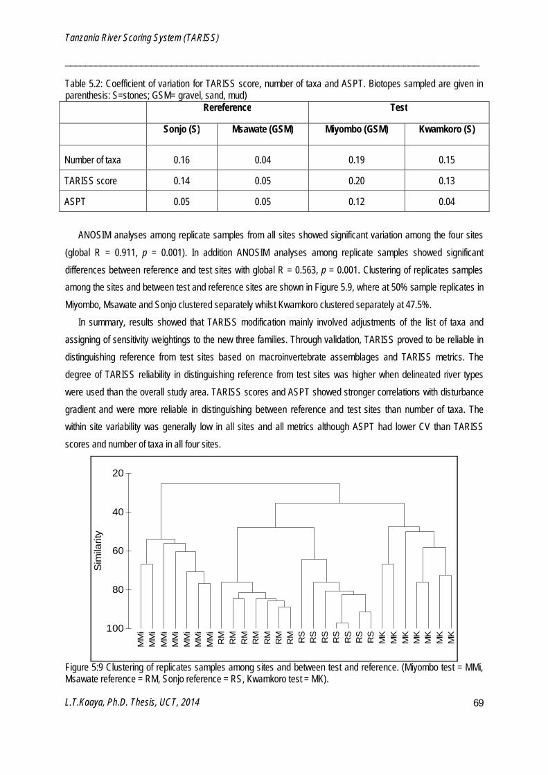
Tanzania River Scoring System (TARISS)
__________________________________________________________________________________
L.T.Kaaya, Ph.D. Thesis, UCT, 2014
69
Table 5.2: Coefficient of variation for TARISS score, number of taxa and ASPT. Biotopes sampled are given in parenthesis: S=stones; GSM= gravel, sand, mud)
Rereference Test
Sonjo (S) Msawate (GSM) Miyombo (GSM) Kwamkoro (S)
Number of taxa 0.16 0.04 0.19 0.15
TARISS score 0.14 0.05 0.20 0.13
ASPT 0.05 0.05 0.12 0.04 ANOSIM analyses among replicate samples from all sites showed significant variation among the four sites
(global R = 0.911, p = 0.001). In addition ANOSIM analyses among replicate samples showed significant differences between reference and test sites with global R = 0.563, p = 0.001. Clustering of replicates samples among the sites and between test and reference sites are shown in Figure 5.9, where at 50% sample replicates in Miyombo, Msawate and Sonjo clustered separately whilst Kwamkoro clustered separately at 47.5%.
In summary, results showed that TARISS modification mainly involved adjustments of the list of taxa and assigning of sensitivity weightings to the new three families. Through validation, TARISS proved to be reliable in distinguishing reference from test sites based on macroinvertebrate assemblages and TARISS metrics. The degree of TARISS reliability in distinguishing reference from test sites was higher when delineated river types were used than the overall study area. TARISS scores and ASPT showed stronger correlations with disturbance gradient and were more reliable in distinguishing between reference and test sites than number of taxa. The within site variability was generally low in all sites and all metrics although ASPT had lower CV than TARISS scores and number of taxa in all four sites.
Group average
MM
iM
Mi
MM
iM
Mi
MM
iM
Mi
MM
iR
MR
MR
MR
MR
MR
MR
M RS
RS
RS
RS
RS
RS
RS
MK
MK
MK
MK
MK
MK
MK
Samples
100
80
60
40
20
Sim
ilarit
y
Figure 5:9 Clustering of replicates samples among sites and between test and reference. (Miyombo test = MMi, Msawate reference = RM, Sonjo reference = RS, Kwamkoro test = MK).
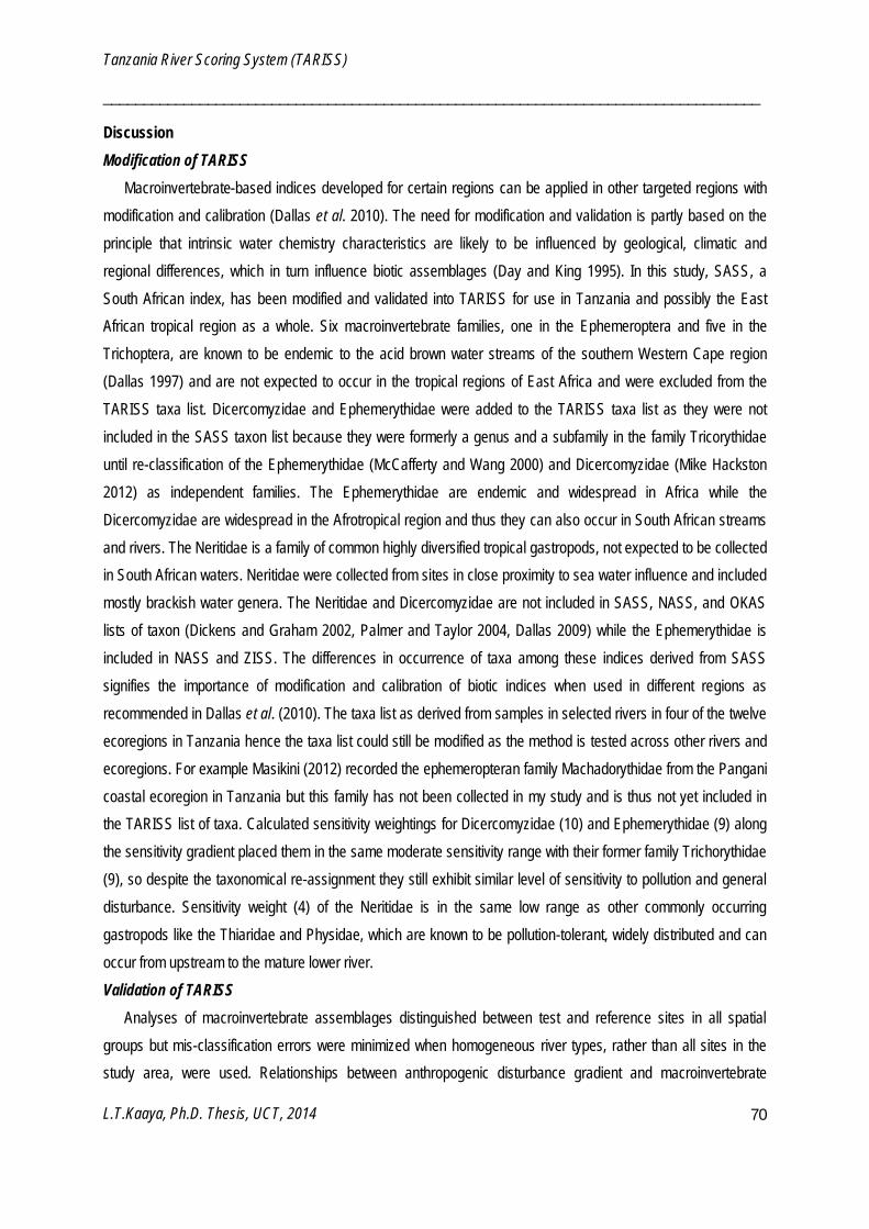
Tanzania River Scoring System (TARISS)
__________________________________________________________________________________
L.T.Kaaya, Ph.D. Thesis, UCT, 2014
70
Discussion Modification of TARISS
Macroinvertebrate-based indices developed for certain regions can be applied in other targeted regions with modification and calibration (Dallas et al. 2010). The need for modification and validation is partly based on the principle that intrinsic water chemistry characteristics are likely to be influenced by geological, climatic and regional differences, which in turn influence biotic assemblages (Day and King 1995). In this study, SASS, a South African index, has been modified and validated into TARISS for use in Tanzania and possibly the East African tropical region as a whole. Six macroinvertebrate families, one in the Ephemeroptera and five in the Trichoptera, are known to be endemic to the acid brown water streams of the southern Western Cape region (Dallas 1997) and are not expected to occur in the tropical regions of East Africa and were excluded from the TARISS taxa list. Dicercomyzidae and Ephemerythidae were added to the TARISS taxa list as they were not included in the SASS taxon list because they were formerly a genus and a subfamily in the family Tricorythidae until re-classification of the Ephemerythidae (McCafferty and Wang 2000) and Dicercomyzidae (Mike Hackston 2012) as independent families. The Ephemerythidae are endemic and widespread in Africa while the Dicercomyzidae are widespread in the Afrotropical region and thus they can also occur in South African streams and rivers. The Neritidae is a family of common highly diversified tropical gastropods, not expected to be collected in South African waters. Neritidae were collected from sites in close proximity to sea water influence and included mostly brackish water genera. The Neritidae and Dicercomyzidae are not included in SASS, NASS, and OKAS lists of taxon (Dickens and Graham 2002, Palmer and Taylor 2004, Dallas 2009) while the Ephemerythidae is included in NASS and ZISS. The differences in occurrence of taxa among these indices derived from SASS signifies the importance of modification and calibration of biotic indices when used in different regions as recommended in Dallas et al. (2010). The taxa list as derived from samples in selected rivers in four of the twelve ecoregions in Tanzania hence the taxa list could still be modified as the method is tested across other rivers and ecoregions. For example Masikini (2012) recorded the ephemeropteran family Machadorythidae from the Pangani coastal ecoregion in Tanzania but this family has not been collected in my study and is thus not yet included in the TARISS list of taxa. Calculated sensitivity weightings for Dicercomyzidae (10) and Ephemerythidae (9) along the sensitivity gradient placed them in the same moderate sensitivity range with their former family Trichorythidae (9), so despite the taxonomical re-assignment they still exhibit similar level of sensitivity to pollution and general disturbance. Sensitivity weight (4) of the Neritidae is in the same low range as other commonly occurring gastropods like the Thiaridae and Physidae, which are known to be pollution-tolerant, widely distributed and can occur from upstream to the mature lower river. Validation of TARISS
Analyses of macroinvertebrate assemblages distinguished between test and reference sites in all spatial groups but mis-classification errors were minimized when homogeneous river types, rather than all sites in the study area, were used. Relationships between anthropogenic disturbance gradient and macroinvertebrate

Tanzania River Scoring System (TARISS)
__________________________________________________________________________________
L.T.Kaaya, Ph.D. Thesis, UCT, 2014
71
assemblages were stronger and thus more reliable when homogenous river types were used compared to the entire study area. In the central eastern Africa uplands river type (CEAU), when macroinvertebrate assemblage data were further classified based on substrate type, and sandy substrate sites from Luwegu sub-catchment were excluded, the mis-classification error was minimized and the differences between test and reference sites increased. This is an important aspect in the application of TARISS because it shows that the less variable macroinvertebrates assemblages among sites are, the more reliable TARISS may be and vice versa, indicating that if natural variability exists among sites, it may influence the functioning of TARISS. Thus when using TARISS, it is important to classify river systems into homogenous regions or river types as frameworks for conducting bioassessment. Reference conditions should be developed for each river type. It is also vital to understand and describe natural variability within different homogenous regions and using this information to analyze and interpret TARISS data. In the CEAU river type, the ability of TARISS to differentiate test from reference sites was reduced by the variability of the substrate, a feature which could lead to inappropriate inferences if not taken into consideration in the analysis and interpretation of TARISS data. Substrate features have been identified as important predictors in the classification of rivers (Dallas 2007a). The GSM biotope in CEAU was mostly dominated by loose sand, which is distinct from stone biotopes in terms of macroinvertebrate assemblages. The exclusion of these sandy sites from the overall CEAU data set increased the separation of test from reference sites.
Cross-validation of the (CAP) Canonical analysis of principal model showed sites that were potentially mis-classified. Sites that were misclassified in PHU, CEAL and CEAU (excluding sandy sites) river types P13, P17 and R01 were mis-classified as test (rather than reference) sites and P28, W01 and W09 were mis-classified as reference (rather than test) sites. Most rivers in the Pangani highlands ecoregion have been severely impacted by a variety of human activities which influences the availability of reference sites thus the best available least disturbed sites such as P13 and P17 were considered as reference sites. R01 was influenced by dam-construction activities upstream of the site between the dry and wet periods of sampling during the course of the study. Thus these three sites, although initially categorized as reference sites, may be in changing from reference to impacted status hence classified as test sites. Sites mis-classified as reference instead of test (P28, W01 and W09), were also least impacted with one major human activity having a direct effect on the site and perhaps influencing ecosystem functioning and biological assemblages. P28 was located downstream of the flower plantation and received agricultural waste products at certain times of the year; and W01 and W09 were influenced by informal settlements where direct activities such as bathing and washing were common. These sites are mainly characterised by local and periodic anthropogenic disturbances. Potential mis-classification of sites brings a challenge to the ability of TARISS to draw conclusions in sites that fall at the boundary or in transition between reference and test status and vice versa. In such sites it is necessary to collect physical and chemical data when collecting macroinvertebrate samples in order to increase the power of detecting anthropogenic impacts. Where disturbances or stressors are minimal, the macroinvertebrate assemblages might
Tanzania River Scoring System (TARISS)
__________________________________________________________________________________
L.T.Kaaya, Ph.D. Thesis, UCT, 2014
72
not change to the extent that TARISS can detect and this should be considered when analyzing and interpreting data from these sites.
TARISS metrics detected changes and showed differences between test and reference sites in all spatial groups. In biological assessment, it is important also to understand how the biotic metrics are correlated with anthropogenic stress (Vlek et al. 2006). Correlation strength reflects the reliability of the metrics. Of the three TARISS metrics, TARIS scores and ASPT correlated more strongly with the anthropogenic disturbance gradient in the overall study area and for all river types indicating that TARISS scores and ASPT are more reliable in depicting anthropogenic impacts than number of taxa. Number of taxa is known to be a poor metric (Karr and Chu 1999) in detecting disturbance. Since both TARISS score and ASPT detected disturbance in all river types during the validation, it is thus recommended that both TARISS score and ASPT be used in interpreting TARISS data. In other words, if a site has either TARISS score or ASPT value within the range of reference condition, then the site should be categorized as a reference site.
As shown that TARISS can be used to detect disturbance by comparisons between reference and test sites, it may also be used to detect changes at a site over time. Some TARISS metrics may be useful for either site to site comparisons or changes over time. While number of taxa is not considered a reliable metric for inter-site comparisons compared to TARISS score and ASPT; it is useful for intra-site comparisons over time. The use of TARISS is dependent on the purpose and aim of the monitoring or assessment. Changes over time might be essential in sites occurring at boundary between reference and test conditions such as sites on transition from recovery to impairment or vice versa. This is because changes at a site over time will give the trend of the site’s condition and unpack the position of the site at the boundary to either reference or test condition. Changes over time, also gives insights to local and periodic disturbances at a site and can be useful in identifying sources of disturbance. However, intra-site comparisons must be separated from influences of natural seasonal variability which highlights up another important aspect in TARISS application. It is thus recommended to examine and characterize seasonal variability and its influence on TARISS for each river type. Within-site sample variability
From the above discussions, natural spatial variability at catchment level and natural temporal variability have featured as potential sources of misinterpreting TARISS data. Furthermore, spatial heterogeneity in micro-habitats at a site has been shown to influence the presence and distribution of macroinvertebrate assemblages (Clarke and Hering 2006) and could be another potential source of misinterpreting TARISS data. Within-biotope variability in macroinvertebrate assemblages may influence the reliability of TARISS metrics. Results showed that ASPT was a less variable metric than TARISS score or number of taxa, perhaps because ASPT is calculated as the ratio of TARISS scores to number of taxa. ASPT should not be affected by the number of replicate samples, possibly because even if only a few taxa are present in a sample they are likely to have appropriate sensitivity scores (Grahams and Dickens 2002). Chutter (1998), Dallas (2000) and Grahams and Dickens (2002) also found ASPT to be a less variable and a more robust metric than number of taxa and SASS score. Number of taxa and
Tanzania River Scoring System (TARISS)
__________________________________________________________________________________
L.T.Kaaya, Ph.D. Thesis, UCT, 2014
73
TARISS score would thus require more replicate samples to achieve less than 10% coefficient of variation than ASPT.
The low coefficient of variation in the Msawate samples can be attributed to the nature of the GSM biotope, comprised of homogenous sandy micro-biotope reaches, which reduced the possibility of under-representation of micro-biotopes among sample replicates. In contrast, Grahams and Dickens (2002) reported GSM as the most variable biotope in terms of scores and number of taxa, perhaps because of the possible varying nature of the percentage of the GSM biotope, which may be comprised of either sand or mud and silt or gravel, affecting the macroinvertebrate assemblages. The composition and quality of GSM biotope may influence the variability of the macroinvertebrate assemblage (Dallas 2007a,b) so TARISS metrics in gravel-dominated GSM are more likely to differ from the sand or mud-dominated GSM. The Miyombo site was under the influence of local anthropogenic disturbances such as bathing, washing and bank erosion, which could have contributed to the higher variability among the replicate samples. GSM in un-impacted homogenous sites can be a less variable and a more reliable biotope than in impacted sites. TARISS, like many other rapid bioassessment methods, uses a single-sample approach for data collection. A single sample, regardless of the method in terms of sampling effort and time, is unlikely to reveal all taxa at a particular site (Nichols et al. 2006). The TARISS sampling approach, of pooling samples from the different biotopes available at a site, reduces the impact of heterogeneity and increases the accuracy of a site sample however. In general, results have shown only a small degree of variability, coefficient of variation being less than or equal to 20% for all TARISS metrics. The important question is whether this variability has an impact on the conclusions regarding river conditions. Clustering of replicate samples within their respective sites (Figure 5.8) showed that the within-site variability among replicate samples is less than the between-site variability. Conclusion and way forward
The validated TARISS technique has proven to be a reliable method for rapid biological assessment of rivers in Tanzania, and probably in the whole East African region. TARISS is designed to be rapid, inexpensive and appropriate for assessment of water quality, general river condition and ecological status in river ecosystems. In addition, TARISS is useful in assessing spatial and temporal trends in river conditions and can serve as a bioassessment tool. TARISS is not intended to identify the nature or type of impact, although it guides physico-chemical water quality monitoring to areas where biological impacts have been detected. TARISS was validated and confirmed for certain ecoregions in Tanzania, therefore there is a need for continuous modification and validation in the other ecoregions in order for TARISS to qualify as a national biotic index. Modification of TARISS in other ecoregions might lead to inclusion of other taxa not currently included in this first version of TARISS. In conclusion TARISS method has been sufficiently validated to be used in other ecoregions in the country.
Several aspects regarding the unbiased, reliable application and interpretation of TARISS which have surfaced include, regional classification, natural spatial and temporal variability, overlapping of sites at the boundary of reference and test conditions and variation in the reliability of different TARISS metrics. Except for
Tanzania River Scoring System (TARISS)
__________________________________________________________________________________
L.T.Kaaya, Ph.D. Thesis, UCT, 2014
74
the regional classification which has been addressed in chapter 4, the remaining issues are indispensable and must be addressed in order for TARISS to be applied as a bioassessment index in Tanzanian. Standard interpretation guidelines for each river type must be developed following river type specific reference conditions. The remaining chapters of this thesis focus on these aspects.
Influence of temporal variation on Bioassessment
__________________________________________________________________________________
L.T.Kaaya, Ph.D. Thesis, UCT, 2014
75
Chapter 6: Influence of Temporal variation on Bioassessment
________________________________________________________________

Influence of temporal variation on Bioassessment
__________________________________________________________________________________
L.T.Kaaya, Ph.D. Thesis, UCT, 2014
76
Introduction
Lotic systems in tropical regions exhibit seasonal variation in hydrology (Lewis 2008) due to climatic seasonality in the form of rainfall which occurs in alternating wet and dry periods (Jacobsen et al. 2008). Hydrological variation is usually associated with seasonal variation in flow, depth and velocity, stream width (e.g Minshall et al. 1985), water chemistry, sediment transport, allochthonous inputs and metabolic rates (e.g. Lewis 2008). Temporal variation in these physical and chemical variables may result in natural temporal variation in macroinvertebrate assemblages. The inherent temporal variation in macroinvertebrate assemblages may influence bioassessment indices or metrics and their interpretation. For instance, comparison of test samples collected in a particular sampling period with reference conditions derived from another sampling period is likely to result in biased conclusions regarding ecological status of the test site (e.g. Linke et al. 1999, Reece et al. 2001). A study by Linke et al. (1999) in Ontario, Canada showed that bioassessment using taxon richness and Family Biotic Index metrics in winter resulted in a higher water quality status than in summer, while a predictive model developed by Reece et al. (2001) in British Columbia using macroinvertebrate reference data from autumn could not be used to accurately predict macroinvertebrates at test sites in other seasons because of seasonal variation.
The primary objective of bioassessment is to detect the degree of impairment on a test site by comparing it to a reference condition. It is important to ensure the accuracy and reliability of the reference condition by understanding the effects of seasonal variability (Dallas 2004a). Temporal variability has been controlled or reduced either by collecting samples within a short period of time (i.e. in established index periods: Barbour et al. 1999) or by combining multiple season samples of a site (Wright 2000). Combined seasons datasets have been shown to increase the prediction accuracy of faunal composition of test sites (Furse et al. 1984). However the increased time and costs of data collection in multiple seasons creates a negative implication in bioassessment. Prior to the application of bioassessment for river health assessment, it is important to examine and characterise temporal variability of biotic assemblages, indices and metrics in order to avoid incorrect inferences. This chapter objectives to 1) to examine temporal variation in TARISS taxa, macroinvertebrate assemblages, number of taxa, TARISS scores and ASPT; and 2) to test the hypothesis that combined seasons reference data increases the accuracy of distinguishing test sites from reference sites’.
Materials and Methods
Macroinvertebrate assemblages
Macroinvertebrates were sampled in wet (long rains and short rains) and dry seasons using the TARISS (Tanzania River Scoring System) sampling protocol as described in chapter 5. Data from three river types namely, Pangani highland uplands (PHU), Central eastern Africa uplands (CEAU) and central eastern Africa lowlands (CEAL) were analysed in combined biotopes data set (stone, vegetation, gravel sand mud) and stone biotopes data set. The three river types were selected because they had adequate number of sites sampled
Influence of temporal variation on Bioassessment
__________________________________________________________________________________
L.T.Kaaya, Ph.D. Thesis, UCT, 2014
77
across seasons. Vegetation and GSM biotopes were not singly analysed because they occurred in fewer sites compared to stones, hence stone biotope and a set of combined biotopes were used.
Data Analysis
Individual taxa
Frequency of occurrence of individual TARISS taxa was calculated separately for the long rains, short rains and dry sampling periods by counting the number of times a taxon occurred among sampling occasions divided by the total number of sampling occasions and expressed as a percentage. Taxa from different biotopes were combined (TARISS total taxa at a site).
Macroinvertebrate assemblages
ANOSIM was used to test the hypothesis that there was no difference in community patterns among the sampling periods within each river type (Clarke and Gorley 2006). Cluster analysis was used to visualize grouping of macroinvertebrate assemblages between wet and dry sampling periods in CEAL because ANOSIM showed significant differences in CEAL only (Clarke and Gorley 2006). SIMPER analyses were used to identify taxa responsible for within–group similarities and between group dissimilarities (Clarke and Gorley 2006). Principle coordinate ordinations were used to show clustering of sites between sampling periods and for exploration of macroinvertebrate taxa contributing to the clustering (Anderson et al. 2008).
Analysis of number of taxa, TARISS scores and ASPT
Number of taxa, TARISS scores and ASPT were compared among the sampling periods using one–way ANOVA after passing the Kolmogorov-Smirnov and Liliefurs test for normality in Statistica at 10 intervals. Number of taxa, TARISS scores and ASPT from single sampling period datasets (i.e. dry, long rains and short rains), were compared with number of taxa, TARISS scores and ASPT calculated from a combined sampling period dataset using one–way ANOVA. Percentage contribution of number of taxa, TARISS scores and ASPT of each sampling period to combined sampling period values were calculated. TARISS metrics from single sampling periods at test sites were compared with metrics from reference data collected in a single period and combined periods for PHU, CEAU and CEAL to compare the two reference datasets.

Influence of temporal variation on Bioassessment
__________________________________________________________________________________
L.T.Kaaya, Ph.D. Thesis, UCT, 2014
78
Results
Frequency of occurrence of TARISS taxa among sampling periods
Frequencies of occurrence of individual TARISS taxa in each sampling period for PHU, CEAU and CEAL are provided in Table 6.1.
Table 6.1: Relative frequency of occurrence (%) of TARISS taxon in the long rains (L), dry (D) and short rains (S) in the Pangani highland uplands (PHU), central eastern Africa uplands (CEAU) and central eastern Africa lowlands (CEAL) river types. (Bold numbers indicate ≥ 50% frequency and shading indicates taxa temporal variation among periods)
PHU CEAU CEAL Order TARISS Taxon L D S L D S L D Turbellaria Turbellaria 10 30 40 0 6 0 0 0 Annelida Oligochaeta 20 10 20 14 22 0 33 21 Hirudinea 10 0 0 7 17 0 8 0 Decapoda Amphipoda 0 0 0 0 0 0 8 0 Potamonautidae 30 50 60 64 67 33 92 79 Atyidae 0 0 0 14 6 0 8 29 Palaemonidae 0 0 0 0 0 0 8 0 Hydrachanellae 10 10 10 7 11 0 8 0 Plecoptera Perlidae 20 30 40 36 44 83 67 43 Ephemeroptera Baetidae 1 sp 10 0 30 29 17 17 17 7 Baetidae 2 sp 0 10 30 14 17 33 8 21 Baetidae >2 sp 80 90 40 64 61 83 75 71 Caenidae 40 60 50 21 61 50 42 29 Heptageniidae 50 50 50 29 33 83 75 43 Leptophlebiidae 40 50 30 50 44 50 83 57 Oligoneuridae 0 10 0 21 33 17 0 7 Polymitarcyidae 10 0 0 14 17 33 0 0 Prosopistomatidae 0 0 0 7 22 17 67 0 Ephemerythidae 20 20 0 29 50 100 58 71 Dicercormyzidae 10 20 0 29 17 0 25 29 Tricorythidae 0 10 0 7 28 0 0 0 Odonata Calopterygidae 0 10 0 29 17 17 17 21 Chlorocyphidae 10 10 0 7 17 67 17 21 Chlorolestidae 0 0 0 7 0 0 0 0 Coenagrionidae 30 60 70 64 61 67 17 79 Lestidae 0 0 0 7 0 0 0 0 Aeshnidae 50 50 50 36 6 17 8 7 Corduliidae 10 30 0 36 44 17 8 29 Gomphidae 60 30 30 86 89 67 75 93
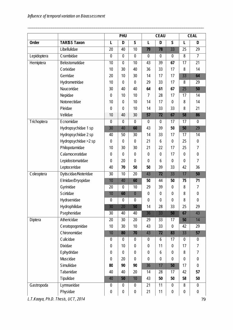
Influence of temporal variation on Bioassessment
__________________________________________________________________________________
L.T.Kaaya, Ph.D. Thesis, UCT, 2014
79
PHU CEAU CEAL Order TARISS Taxon L D S L D S L D Libellulidae 20 40 10 79 78 33 25 29 Lepidoptera Crambidae 0 0 0 0 0 0 8 7 Hemiptera Belostomatidae 10 0 10 43 39 67 17 21 Corixidae 10 30 40 36 33 17 8 14 Gerridae 20 10 30 14 17 17 33 64 Hydrometridae 10 0 0 29 33 17 8 29 Naucoridae 30 40 40 64 61 67 25 50 Nepidae 0 10 10 7 28 17 17 14 Notonectidae 10 0 10 14 17 0 8 14 Pleidae 0 0 10 14 33 33 8 21 Veliidae 10 40 30 57 72 67 58 86 Trichoptera Ecnomidae 0 0 0 0 0 17 17 0 Hydropsychidae 1 sp 30 40 60 43 39 50 50 29 Hydropsychidae 2 sp 40 50 30 14 33 17 17 14 Hydropsychidae >2 sp 0 0 0 21 6 0 25 0 Philopotamidae 10 30 30 21 22 17 25 7 Calamoceratidae 0 0 0 0 0 17 0 0 Lepidostomatidae 0 20 0 0 6 0 0 7 Leptoceridae 40 70 50 50 39 33 42 36 Coleoptera Dytiscidae/Noteridae 30 10 20 43 72 33 17 50 Elmidae/Dryopidae 10 40 60 50 44 50 75 71 Gyrinidae 20 0 10 29 39 0 8 7 Scirtidae 10 60 0 0 0 0 8 0 Hydraenidae 0 0 0 0 0 0 8 0 Hydrophilidae 30 20 50 14 28 33 25 29 Psephenidae 30 40 40 36 33 50 67 43 Diptera Athericidae 20 30 20 29 33 17 50 14 Ceratopogonidae 10 30 10 43 33 0 42 29 Chironomidae 10 80 70 43 72 83 33 57 Culicidae 0 0 0 0 6 17 0 0 Dixidae 0 10 0 0 11 0 17 7 Ephydridae 0 0 0 0 6 0 8 7 Muscidae 0 20 0 0 0 0 0 0 Simuliidae 80 90 90 36 17 50 17 0 Tabanidae 40 40 20 14 28 17 42 57 Tipulidae 40 50 10 43 50 50 58 50 Gastropoda Lymnaeidae 0 0 0 21 11 0 8 0 Physidae 0 0 0 21 11 0 0 0
Influence of temporal variation on Bioassessment
__________________________________________________________________________________
L.T.Kaaya, Ph.D. Thesis, UCT, 2014
80
PHU CEAU CEAL Order TARISS Taxon L D S L D S L D Planorbinae 0 30 20 0 11 0 0 0 Thiaridae 0 0 0 7 17 0 0 0
Many taxa occurred in all sampling periods for all river types while a few taxa were present or absent, or occurred more or less frequently in certain sampling periods. In PHU, CEAU and CEAL, 10, 7 and 13 taxa respectively showed temporal preferences by occurring in higher frequencies in a particular sampling period. In PHU and CEAU the majority of taxa that indicated temporal preferences occurred at lower frequencies in the long rains than in the short rains and dry periods. In CEAL, taxa associated with stone and fast flowing biotopes such as the Perlidae, Heptageniidae, Leptophlebiidae, Prosopistomatidae, Psephenidae and Athericidae occurred at higher frequencies during the wet than dry period. On the contrary, vegetation-associated taxa such as the Coenogrionidae and Naucoridae and slow flow, stream edges and pools associated taxa such as the Gerridae, Veliidae, Chironomidae and Dytiscidae occurred in higher frequencies during dry period than the wet period. Prosopistomatidae did not occur in the dry period in CEAL. Only five taxa showed temporal preferences in more than one river type. The Coenogrionidae, Velidae and Dytiscidae occurred in higher frequencies in the dry period, the Hepategeniidae occurred in higher frequencies in wet periods and the Chironomidae occurred in higher frequencies in the dry period in CEAL, and in dry and short periods in PHU and CEAU. Potamonautidae, Chironomidae, Gomphidae, Leptophlebiidae, Coenogrionidae, Baetidae > 2sp, Elmidae, Tipulidae and Veliidae occurred in higher frequencies among the sampling periods than other taxa in all river types.
Temporal variation in macroinvertebrate assemblages
Macroinvertebrate assemblages did not show any temporal variation among the sampling periods in PHU (global R = 0.009, p = 0.401 and global R = 0.04, p = 0.204) or CEAU (global R = 0.015, p = 0.326 and global R = 0.104, p = 0.051) in both combined biotopes and stone biotope respectively In contrast, in the CEAL, macroinvertebrate assemblages showed significant temporal differences between the wet and dry periods in both combined and stone biotopes (global R = 0.201, p = 0.005 and global R = 0.034, p = 0.001 respectively). Cluster analysis in CEAL illustrates grouping patterns of macroinvertebrate assemblages in combined biotopes and stone biotope (Figure 6.1). Analyses for similarity levels within the wet and dry periods were performed using SIMPER analysis by the Bray-Curtis similarity with a 90% cut off for low contributions. In combined biotopes analysis, within–wet period similarity was 50.74% contributed by Potamonautidae, Leptophlebiidae, Gomphidae, Elmidae, Heptageniidae and Prosopistomatidae and the within–dry period similarity was 53.38% contributed by Gomphidae, Potamonautidae, Veliidae, Ephemerythidae, Coenogrionidae and Baetidae >2sp. Analysis of stone biotope dataset revealed stronger differences between the wet and dry periods with the within-wet period similarity of 62.76% contributed by Potamonautidae, Leptophlebiidae, Prosopistomatidae, Psephenidae,
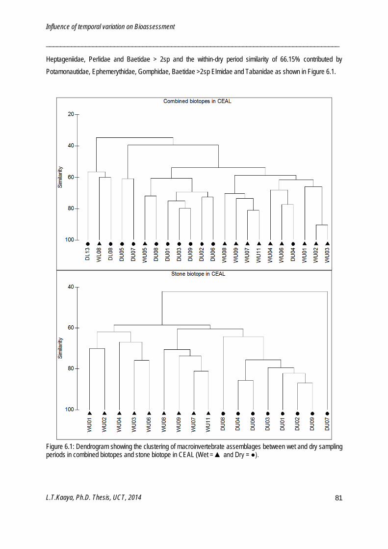
Influence of temporal variation on Bioassessment
__________________________________________________________________________________
L.T.Kaaya, Ph.D. Thesis, UCT, 2014
81
Heptageniidae, Perlidae and Baetidae > 2sp and the within-dry period similarity of 66.15% contributed by Potamonautidae, Ephemerythidae, Gomphidae, Baetidae >2sp Elmidae and Tabanidae as shown in Figure 6.1.
Figure 6.1: Dendrogram showing the clustering of macroinvertebrate assemblages between wet and dry sampling periods in combined biotopes and stone biotope in CEAL (Wet = ▲ and Dry = ●).
Influence of temporal variation on Bioassessment
__________________________________________________________________________________
L.T.Kaaya, Ph.D. Thesis, UCT, 2014
82
Temporal variation in TARISS metrics
In the combined biotopes, the only significant difference in TARISS metrics amongst sampling periods was for ASPT in PHU (F = 3.504, p = 0.0407) and CEAL (t = 2.896, p = 0.0084, DF = 22). In the stone biotope, significant differences between wet and dry sampling periods were found in CEAL only for number of taxa (t = 2.565, p = 0.0215, DF = 15), TARISS scores (t = 3.971, p = 0.0012, DF = 15) and ASPT (U’ = 60, p = 0.0206).
Comparisons of TARISS metrics between single sampling periods (i.e. dry, long rains and short rains) and combined sampling periods using combined biotope data sets for PHU showed significant differences between single and combined sampling periods in the number of taxa (p = 0.0008, F = 6.954) and TARISS scores (p = 0.0009, F = 6.917) where significant differences were between the combined period and long rains and short rains. No significant differences were found between metrics for the combined period and dry period’s metrics. In CEAU significant differences occurred only in the number of taxa (p = 0.0016, F = 5.853) between combined periods and dry and long rains while in CEAL there were no significant differences between combined periods and dry or wet periods in either number of taxa (p = 0.1318, F = 2.145) nor TARISS score (p = 0.1145, F = 2.303). ASPT only varied between wet and dry periods in CEAL (p = 0.01, F = 5.249). Combined sampling period’s data resulted in more significant differences between reference and test sites than did single sampling period’s data for all seasons. Significant differences were in the number of taxa and TARISS score in PHU, and in the number of taxa, TARISS score and ASPT in CEAL (Table 6.2). Table 6.2 gives a summary of statistical comparison between reference and test metrics.

Influence of temporal variation on Bioassessment
__________________________________________________________________________________
L.T.Kaaya, Ph.D. Thesis, UCT, 2014
83
Table 6.2: One-way analysis of variance (ANOVA) of TARISS metrics between combined periods, long rains, dry, short rains references and long rains, dry, short rains test sites. The Turkey-Kramer multiple comparison test (q) determined significant differences between groups in PHU and CEAL. Shaded cells indicate comparisons with significant differences. (CR= Combined periods reference, LR = long rains reference, SR = short rains reference, DR = dry reference, LT = long rains test, ST = short rains test, DT = dry test). PHU q p CEAL q p
Number of Taxa
CR vs LT 8.229 <0.001 CR vs LT 8.68 <0.001 CR vs DT 9.842 <0.001 CR vs DT 6.783 <0.001 CR vs ST 7.94 <0.001 LR vs LT 0.207 >0.05 LR vs LT 5.274 <0.001 LR vs T 1.856 >0.05 LR vs T 3.085 >0.05 LR vs ST 0.7575 >0.05 DR vs LT 3.125 >0.05 DR vs LT 5.94 <0.001 DR vs DT 4.774 <0.05 DR vs DT 3.814 >0.05 DR vs ST 3.307 >0.05
SR vs LT 1.729 >0.05 SR vs DT 3.378 >0.05 SR vs ST 2.088 >0.05
TARISS Score
CR vs LT 9.126 <0.001 CR vs LT 9.457 <0.001 CR vs DT 10.548 <0.001 CR vs DT 8.597 <0.001 CR vs ST 8.631 <0.001 LR vs LT 1.547 >0.05 LR vs LT 6.903 <0.001 LR vs DT 2.962 >0.05 LR vs DT 5.799 <0.001 LR vs ST 2.008 >0.05 DR vs LT 4.696 <0.05 DR vs LT 6.303 <0.001 DR vs DT 6.118 <0.05 DR vs DT 5.142 <0.001 DR vs ST 4.76 <0.05
SR vs LT 2.125 >0.05 SR vs DT 3.548 >0.05 SR vs ST 2.514 >0.05
ASPT
CR vs LT 2.817 >0.05 CR vs LT 5.476 <0.001 CR vs DT 4.337 <0.05 CR vs DT 7.356 <0.001 CR vs ST 2.581 >0.05 LR vs LT 3.583 >0.05 LR vs LT 7.65 <0.001 LR vs DT 5.103 <0.01 LR vs DT 9.669 <0.001 LR vs ST 3.25 >0.05 DR vs LT 3.77 >0.05 DR vs LT 4.19 <0.05 DR vs DT 5.289 <0.01 DR vs DT 5.858 <0.001 DR vs ST 3.413 >0.05
SR vs LT 1.503 >0.05 SR vs DT 3.023 >0.05 SR vs ST 1.433 >0.05
Influence of temporal variation on Bioassessment
__________________________________________________________________________________
L.T.Kaaya, Ph.D. Thesis, UCT, 2014
84
Discussion
Temporal variation of aquatic macroinvertebrates in the tropical east African region is poorly known and the literature is limited to a few studies e.g. Mathooko and Mavuti (1992), Shivoga (2001), Jacobsen et al. (2008). This paucity of information necessitated the investigation of temporal variability in macroinvertebrates assemblages and the potential influence of this variability on the performance of TARISS in assessing conditions in river and stream ecosystems. The majority of tropical stream insects have semi-continuous or year-round reproductive cycles almost independent of seasons, although, some show strong seasonality, usually related to stream-flow patterns (Mathooko 1996 in Jacobsen et al. 2008, Jacobsen et al. 2008).
In this study, major temporal variation in the frequency of occurrence of individual TARISS taxa among different sampling periods was limited to a few taxa and varied among river types. Higher frequencies of lithophilic taxa in the wet period than the dry period may be due to influences of changes in flow regime or availability of stony biotopes as well as their stability. The Perlidae, Heptageniidae, Leptophlebiidae, Prosopistomatidae, Psephenidae, Athericidae and Hydropsychidae are all known to occur in stony or rocky substrate in moderately to fast-flowing streams. In the wet period, flow depth and velocity increase hence availability of riffles increased, and supported the occurrence and dominance of these taxa. For example, the Prosopistomatidae, which showed a marked occurrence in the wet period only in CEAL, is known to be lithophilic and rheophilic because its distribution is driven primarily by substratum and current features (Schletterer and Fureder 2009). In contrast, higher frequencies of the Coenogrionidae, Gerridae, Naucoridae, Veliidae, Dytiscidae and Chironomidae that inhabit vegetation, stream edges and pools may also be associated with reduction in flow which supports availability of vegetation, and pool associated habitats. In addition, allochthonous materials such as leaves and twigs accumulated during the dry period as a result of slow transport of materials due to low flow velocity may have provided food and surfaces for attachment of these taxa (Mathooko and Mavuti 1992).
In East African tropical region, flow regime and habitat stability as functions of seasonality, have a primary influence on macroinvertebrate life cycles and population dynamics (Jacobsen et al. 2008); temperature is less important because of minimal variability in mean annual temperatures (Griffiths 1972, Mwamende 2009). The seasonal variability in the frequency of occurrence of TARISS taxa in this study is important in biological assessment of rivers and streams because taxa with higher frequencies in the wet period tend to be the more sensitive taxa (sensitivity weightings of 10 – 15) while the dry period is dominated by more tolerant taxa (sensitivity weightings of 2 – 7). This means the wet period samples will reflect a higher ecological category than the dry period samples at the same site leading to two different ecosystem status values. Understanding and considering the temporal variation in the three regions of this study assist in the interpretation of bioassessment data, and allow for temporal variability to be accounted for in bioassessment.
Macroinvertebrate assemblages showed temporal variation only in CEAL and did not vary significantly in PHU or CEAU. These results can be explained by the frequency of occurrence results, where more taxa in CEAL
Influence of temporal variation on Bioassessment
__________________________________________________________________________________
L.T.Kaaya, Ph.D. Thesis, UCT, 2014
85
showed temporal variation than in PHU and CEAU. Furthermore, CEAL was the only river type that included sites from unimodal rainfall regions which have one rainy sampling period and one dry period. Truly seasonal conditions in the tropics occur in rivers within the moonsonal regions where there are marked wet and dry periods (Jacobsen et al. 2008). Unimodal rainfall patterns generate a stronger difference between the wet and dry periods than bimodal rainfall patterns where the difference between the wet and dry period is reduced by the short rains. Marked seasonal conditions transform into marked seasonal changes in flow regime, sediment transport, allochthonous materials supply, habitat availability and stability which in the end define macroinvertebrate life histories and distribution. As a result, macroinvertebrate taxon composition changes less annually in bimodal regions than in unimodal regions. This is relevant to the issue of appropriate TARISS sampling period. The choice of when TARISS samples are collected should be determined based on the rainfall pattern at a given region and the knowledge of differences in macroinvertebrate assemblages brought by the wet and dry period cycles should be considered in the interpretation of data.
Examination of macroinvertebrates assemblages in the CEAL stone biotope resulted in a clearer differentiation between the rainy and dry periods than when combined biotopes were used, possibly because the stone biotope is more sensitive to flow regime changes than the other biotopes are (Dallas 2002). Dallas (2002) found stronger differences in macroinvertebrate assemblages in stone-associated biotopes between spring and autumn periods in South Africa than in combined biotopes. In this study, when stone biotope sample was used, the taxa contributing to within group similarity in the wet period included more taxa associated with stone, fast flowing biotope than in combined biotopes. This resulted in increased differences between the wet and dry sampling periods compared to when combined biotopes was used CEAL substrata were characterised by gravel and small stones including pebbles and cobbles. Taxa such as Perlidae and Prosopistomatidae, which showed differences in occurrence between wet and dry periods, are known to occur in gravel, pebble and small stone dominated habitats (Ogbogu 2006, Schletterer and Fureder 2009) and so any flow changes might have an impact on the stone biotope and hence on their occurrence and distribution.
Seasonal changes in macroinvertebrate assemblages have been found to have marked effects on many biotic indices (e.g. Reece et al. 2001, Sporka et al. 2006). Invertebrate life cycles and changes in macroinvertebrate composition may affect bioassessment metrics. Observed temporal variation in macroinvertebrate taxa and assemblages in this study have also influenced the ASPT in PHU and CEAL with combined biotopes, and the number of taxa, TARISS scores and ASPT in CEAL when stone biotopes were used. These marked differences between the wet and dry periods in TARISS reference metrics bring an alert to the use of reference conditions for comparison with test sites. Reference conditions should be able to differentiate natural temporal variation from variation caused by human disturbance and stressors. As a consequence, test sites from wet period should be compared to wet period reference conditions and test sites from dry period should be compared to dry period reference conditions. In this way hydrology is taken into account, and potential biases associated with hydrological changes are accounted for.

Influence of temporal variation on Bioassessment
__________________________________________________________________________________
L.T.Kaaya, Ph.D. Thesis, UCT, 2014
86
Because of spatio-temporal variation in macroinvertebrate assemblages, Ormerod (1987) suggested that the most accurate data set of macroinvertebrate assemblages involves sampling that combines both habitat and seasonal data. Results from this study support the higher precision in using combined biotopes and sampling periods reference conditions for detecting changes in test sites. In all TARISS metrics, combined spatial and temporal reference data set resulted in higher significances of variation from test sites of all three sampling periods, suggesting that it is a more reliable and possibly accurate way of categorising the types of macroinvertebrate data in river systems.
Understanding natural variability in macroinvertebrate taxa and TARISS metrics is important in monitoring programmes of river and stream ecosystems where a particular site is examined for changes over a period of time i.e. annually. In such a situation, temporal changes can easily be mis-interpreted for changes due to anthropogenic impacts. Thus in regions where temporal variability is apparent, e.g. CEAL, monitoring programmes should be conducted over a period of time and seasonal reference conditions should be used to detect and interpret changes at a site.
It is recommended that, in order to account for temporal variability when using TARISS it is important to ascertain the presence of significant temporal variability in TARISS metrics among the main seasons in a particular region. If there are no significant temporal differences among seasons, then a combined-seasonal reference condition should be used. In cases where there are significant differences among seasons, it is best recommended to use season-specific reference conditions to detect changes in their respective test sites. However, even for sites where seasonal differences in TARISS metrics exists, combined reference metrics are also suitable for use in situations where development of seasonal reference conditions is not feasible. The use of combined reference condition approach is useful in bioassessment as one combined reference condition can be used to compare data from all sampling periods. Another advantage of a reference condition developed from multiple sampling periods is that it reduces challenges of deciding a suitable time period for sampling, since a test sample from any time of the year can be compared with a single set of reference conditions. Another option in regions were seasonal variations exists is to conduct bioassessment only during one season and use a single season established reference condition.
Ways to account for temporal variation in the development and application of TARISS reference conditions and interpretation guidelines are detailed in the next chapter.
Influence of spatial variation on TARISS Reference Conditions
__________________________________________________________________________________
L.T.Kaaya, Ph.D. Thesis, UCT, 2014
87
Chapter 7: Influence of Spatial variation on TARISS Reference Conditions
________________________________________________________________

Influence of spatial variation on TARISS Reference Conditions
__________________________________________________________________________________
L.T.Kaaya, Ph.D. Thesis, UCT, 2014
88
Introduction
Rivers are generally heterogeneous and complex systems because of spatial and temporal variability in abiotic and biotic variables and their interaction at different scales. Spatial variability occurs in rivers at multiple scales namely, catchment such as longitude, latitude, altitude, geology, climate and catchment area (Richards et
al. 1997, Turak et al. 1999), habitat such as substrate type, substrate composition, biotope availability and abundance (Reynoldson et al. 1997, Collier et al. 1999) and site characteristics such as flow pattern, canopy cover (Kay et al .1999, Dallas 2007b), stream depth, stream width, flow and velocity (Poff and Ward 1990). Macroinvertebrate assemblages are known to be influenced by spatial and temporal variability in river systems, hence their heterogeneity and patchy distribution (Poff and Ward 1990, Palmer and Poff 1997, Dallas 2004b, Dallas 2007a). Additional variables that may also influence macroinvertebrate assemblages under natural conditions include oxygen levels, electrical conductivity, pH, nutrient concentrations and water temperature (Collier 1995, Hawkins et al.1997, Dallas and Day 2004). In the context of bioassessment, reliable and unbiased interpretation of assessment data and derived conclusions are important aspects. One approach to meaningful and unbiased interpretation of biological data is based on the assessment of influential environmental variables that best explain biological assemblages in a region. Because of this, it is crucial to characterise and identify environmental variables that best describe macroinvertebrate assemblages under natural conditions when establishing reference conditions.
There is limited published information on spatial and temporal variability in river systems and macroinvertebrate assemblages in Tanzania. Regional classification of Tanzanian rivers, as described in chapter 4, resulted in spatially variable 12 ecoregions, 36 slope classes and 144 geomorphologic landforms based on climatic and geomorphologic characteristics. The above results from chapter 4 indicate the presence of spatial variability in river systems and possibly therefore of macroinvertebrate taxa and assemblages in Tanzanian rivers. Information on spatial variability in river systems and macroinvertebrate assemblages, and how such variability may influence development and use of TARISS reference conditions, forms the basis of this chapter. In this chapter, I investigate the spatial variability in environmental variables in three river types and how such variability influences variability in metrics relating to macroinvertebrate assemblages: number of taxa, TARISS scores and ASPT values. The influence of variability on the number of taxa, TARISS scores and ASPT values on the development of reference conditions and detection of disturbance at impaired sites has been examined.
In this chapter, guidelines for interpretation of TARISS data will be established by developing “biological bands”, identifying taxa expected in reference conditions and giving trends of taxon occurrence between reference and impaired conditions. A biological band is an ecosystem status category in terms of human disturbance defined by a range of TARISS scores and ASPT values derived by percentiles of a biotic data set.
Therefore this chapter objectives 1) to examine the spatial variability of environmental variables 2) to examine if spatial variability in environmental variables influences the TARISS metrics 3) to develop and validate TARISS
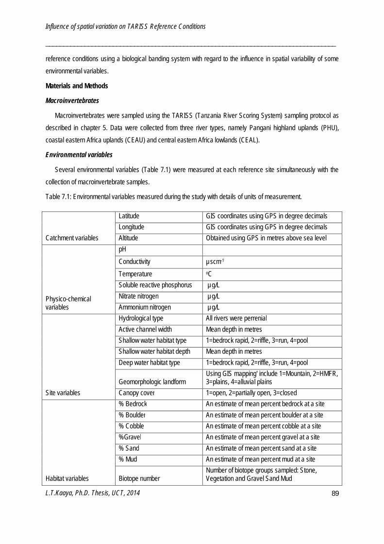
Influence of spatial variation on TARISS Reference Conditions
__________________________________________________________________________________
L.T.Kaaya, Ph.D. Thesis, UCT, 2014
89
reference conditions using a biological banding system with regard to the influence in spatial variability of some environmental variables.
Materials and Methods
Macroinvertebrates
Macroinvertebrates were sampled using the TARISS (Tanzania River Scoring System) sampling protocol as described in chapter 5. Data were collected from three river types, namely Pangani highland uplands (PHU), coastal eastern Africa uplands (CEAU) and central eastern Africa lowlands (CEAL).
Environmental variables
Several environmental variables (Table 7.1) were measured at each reference site simultaneously with the collection of macroinvertebrate samples.
Table 7.1: Environmental variables measured during the study with details of units of measurement.
Catchment variables
Latitude GIS coordinates using GPS in degree decimals Longitude GIS coordinates using GPS in degree decimals Altitude Obtained using GPS in metres above sea level
Physico-chemical variables
pH Conductivity µscm-1 Temperature oC Soluble reactive phosphorus µg/L Nitrate nitrogen µg/L Ammonium nitrogen µg/L
Site variables
Hydrological type All rivers were perrenial Active channel width Mean depth in metres Shallow water habitat type 1=bedrock rapid, 2=riffle, 3=run, 4=pool Shallow water habitat depth Mean depth in metres Deep water habitat type 1=bedrock rapid, 2=riffle, 3=run, 4=pool
Geomorphologic landform Using GIS mapping' include 1=Mountain, 2=HMFR, 3=plains, 4=alluvial plains
Canopy cover 1=open, 2=partially open, 3=closed
Habitat variables
% Bedrock An estimate of mean percent bedrock at a site % Boulder An estimate of mean percent boulder at a site % Cobble An estimate of mean percent cobble at a site %Gravel An estimate of mean percent gravel at a site % Sand An estimate of mean percent sand at a site % Mud An estimate of mean percent mud at a site
Biotope number Number of biotope groups sampled: Stone, Vegetation and Gravel Sand Mud

Influence of spatial variation on TARISS Reference Conditions
__________________________________________________________________________________
L.T.Kaaya, Ph.D. Thesis, UCT, 2014
90
Environmental variables were grouped into four categories namely, catchment (longitude, latitude, altitude and geological landform), site (shallow water habitat type, shallow water habitat depth, deep water habitat type and deep water habitat depth, active channel width and canopy cover), habitat (percentage cover of bedrock, boulders, cobbles, gravel, sand, mud and number of biotopes sampled) and water chemistry (pH, electrical conductivity, water temperature, soluble reactive phosphorous, nitrate and ammonium nutrients).
Data Analysis
Macroinvertebrate assemblages
Cluster and MDS analyses were used to examine and visualize grouping of sites based on macroinvertebrate assemblages (Clarke and Gorley 2006). Analyses were done separately for combined biotopes, stone biotope, vegetation biotope and GSM biotope in PHU, CEAU and CEAL. One-way analysis of similarities (ANOSIM) was used to test whether or not there were significant differences among groups based on macroinvertebrate assemblages (Clarke and Gorley 2006). Data from different sampling periods were combined into one data set. In chapter 6, based on results, the use of combined season data set was recommended over use of single season data sets. Taxa responsible for within-group similarity, and dissimilarity between groups, were identified using SIMPER analysis (Clarke and Gorley 2006).
Environmental variables
Environmental variables distinguishing groups of sites with similar macroinvertebrate assemblages were identified in PHU, CEAU and CEAL using stepwise Discriminant Function Analysis (DFA). Data from separate sampling periods were averaged to one data set for each site. Only groups formed by combined biotope data sets were used in the DFA analysis. Prior to DFA, variables were compared among groups using a one-way ANOVA and only variables that showed significant differences (p<0.005) among groups were considered for DFA analysis. Variables that contributed most to the discrimination were identified by DFA coefficient Partial Wilk’s Lambda which measures the discriminatory power. Partial Wilk’s Lambda ranges from 0 to 1 where 0 = perfect discriminatory power and 1 = no discriminatory power Predictive classification for each group was examined and predictive percentage correctness errors were noted.
Derivation of biological bands
Macroinvertebrate assemblages from reference and test sites were used to derive biological bands in each river type. Combined data sets for all sampling periods were used for reference sites while for test sites, data sets from separate sampling periods were used. Prior to developing biological bands, variability of TARISS metrics were examined by calculating minimum, median, maximum, 90th,67.5th, 45th and 22.5th percentiles of number of taxa, TARISS scores and ASPT.
A biological banding system which uses variability in absolute scores and ASPT values as described in Dallas (2007) and Dallas and Day (2007) was used to develop biological bands in each river type.
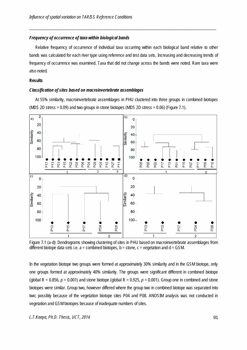
Influence of spatial variation on TARISS Reference Conditions
__________________________________________________________________________________
L.T.Kaaya, Ph.D. Thesis, UCT, 2014
91
Frequency of occurrence of taxa within biological bands
Relative frequency of occurrence of individual taxa occurring within each biological band relative to other bands was calculated for each river type using reference and test data sets. Increasing and decreasing trends of frequency of occurrence was examined. Taxa that did not change across the bands were noted. Rare taxa were also noted.
Results
Classification of sites based on macroinvertebrate assemblages
At 55% similarity, macroinvertebrate assemblages in PHU clustered into three groups in combined biotopes (MDS 2D stress = 0.09) and two groups in stone biotopes (MDS 2D stress = 0.06) (Figure 7.1).
Figure 7.1 (a-d): Dendrograms showing clustering of sites in PHU based on macroinvertebrate assemblages from different biotope data sets i.e. a = combined biotopes, b = stone, c = vegetation and d = GSM.
In the vegetation biotope two groups were formed at approximately 30% similarity and in the GSM biotope, only one groups formed at approximately 40% similarity. The groups were significant different in combined biotope (global R = 0.856, p = 0.001) and stone biotope (global R = 0.925, p = 0.001). Group one in combined and stone biotopes were similar. Group two, however differed where the group two in combined biotope was separated into two; possibly because of the vegetation biotope sites P04 and P08. ANOSIM analysis was not conducted in vegetation and GSM biotopes because of inadequate numbers of sites.

Influence of spatial variation on TARISS Reference Conditions
__________________________________________________________________________________
L.T.Kaaya, Ph.D. Thesis, UCT, 2014
92
Macroinvertebrate assemblages in CEAU clustered into three groups at approximate 44% similarity in combined biotopes (MDS 2D stress = 0.17), two groups at approximate 55% similarity in stone biotope (MDS 2D stress = 0.08), three groups at approximate 48% in vegetation (MDS 2D stress = 0.16) and in two groups at approximate 25% similarity in GSM (MDS 2D stress = 0.10) as shown in Figure 7.2. The groups were significant different in combined biotopes (global R = 0.564, p = 0.001), stone (global R = 0.876, p = 0.002), vegetation (global R = 0.630, p = 0.001) and GSM (global R = 0.627, p = 0.001).
Figure 7.2 (a-d): Dendrograms showing clustering of sites in CEAU based on macroinvertebrate assemblages from different biotope data sets i.e. a = combined biotopes, b = stone, c = vegetation and d = GSM.
Macroinvertebrate assemblages in CEAL clustered sites into three groups at 50% similarity in combined biotopes (MDS 2D stress = 0.11), two groups at 37% similarity in vegetation (MDS 2D stress = 0.17) and two groups at 35% similarity in GSM (MDS 2D stress = 0.05) as shown in Figure 7.3. In stone biotope all sites are similar at approximately 70% (MDS 2D stress = 0.11). The groups were significant different in combined biotopes (global R = 0.918, p = 0.002), vegetation (global R = 0.588, p = 0.001) and GSM (global R = 0.778, p = 0.014). Sites L08 and L09 were consistently in group two in the combined biotopes, vegetation and GSM biotope.
Influence of spatial variation on TARISS Reference Conditions
__________________________________________________________________________________
L.T.Kaaya, Ph.D. Thesis, UCT, 2014
93
Figure 7.3 (a-d): Dendrograms showing clustering of sites in CEAL based on macroinvertebrate assemblages from different biotope data sets i.e. a = combined biotopes, b = stone, c = vegetation and d = GSM.
In PHU, the stone classification was more similar to the combined classification than the vegetation and GSM classifications; in CEAL, stone, vegetation and GSM classifications all showed strong resemblance to the combined classification; while in CEAU, none of the single biotope classifications showed clear resemblance to the combined classification. Results of classifications in PHU and CEAL suggests differentiation of sites between sub catchments within respective river types. Within-group similarity of macroinvertebrates assemblages in the combined data sets was more than 50% in all groups formed within each river type (Table 7.2). Highest dissimilarity was between group one and three (63.87%) in PHU, between group two and three in CEAU (61.88%) and between group one and two in CEAL (62.29%). Taxa that contributed to the grouping of sites among river types in the combined data sets were identified and are shown in Table 7.2.
Influence of spatial variation on TARISS Reference Conditions
__________________________________________________________________________________
L.T.Kaaya, Ph.D. Thesis, UCT, 2014
94
Table 7.2: List of taxa contributing to 90% within-group similarity of groups formed by reference sites from PHU, CEAU and CEAL using SIMPER analysis. Taxa contributing to the first 50% similarity are indicated by▲and taxa contributing to the remaining 40%percent similarity are indicated by □.
PHU CEAU CEAL Group 1 2 3 1 2 3 1 2 3 % Similarity 65.67 63.21 72.00 53.43 57.17 58.06 67.26 61.22 62.02 Aeshnidae ▲ ▲ □ Ancylidae □ □ □ □ Athericidae ▲ □ □ Baetidae >2sp ▲ ▲ ▲ ▲ ▲ ▲ ▲ Belostomatidae □ ▲ Caenidae ▲ □ □ ▲ ▲ Ceratopogonidae □ □ Chironomidae □ ▲ □ □ ▲ Chlorocyphidae ▲ Coenagrionidae □ ▲ ▲ ▲ □ ▲ Corduliidae □ ▲ Corixidae □ ▲ Culicidae □ □ □ □ Dicercormyzidae □ Dytiscidae □ □ □ □ Ecnomidae □ Elmidae □ □ □ □ Ephemerythidae □ ▲ ▲ Gerridae □ □ ▲ Gomphidae ▲ ▲ ▲ ▲ ▲ ▲ ▲ ▲ Gyrinidae □ ▲ □ □ Heptageniidae ▲ ▲ Hydrachanellae □ Hydraenidae □ ▲ Hydropsychidae 1 sp □ □ Hydropsychidae 2 sp □ ▲ □ Hydrophilidae □ □ Leptoceridae □ ▲ □ □ Leptophlebiidae ▲ □ □ ▲ ▲ ▲ ▲ Libellulidae □ ▲ ▲ ▲ ▲ ▲ Lymnaeidae □ Naucoridae ▲ ▲ □ □ □ Nepidae □ □
Influence of spatial variation on TARISS Reference Conditions
__________________________________________________________________________________
L.T.Kaaya, Ph.D. Thesis, UCT, 2014
95
Notonectidae □ □ Oligochaeta □ □ Perlidae □ ▲ □ Philopotamidae □ Pleidae □ □ Potamonautidae ▲ □ ▲ ▲ ▲ Prosopistomatidae □ ▲ Psephenidae □ □ Syrphidae □ □ □ □ Tabanidae □ Tipulidae □ ▲ Tricorythidae □ Turbellaria □ Veliidae □ ▲ ▲ □ □ □
Variability in number of taxa, TARISS scores and ASPT values
Minimum, median, maximum, first and third percentiles for number of taxa, TARISS scores and ASPT for macroinvertebrate groups formed with reference sites in PHU, CEAU and CEAL are shown in Figure 7.4-7.6. The percentile values are provided in appendix 7.1. In PHU, group two varied less than combined group two and three in number of taxa, TARISS scores and ASPT. Generally, ASPT was least varying than number of taxa and TARISS scores in PHU (Figure 7.4). In CEAU, group two varied least in number of taxa, TARISS scores and ASPT while group one was most variable in all metrics. Combined group two and three was slightly more varying than group two in ASPT (Figure 7.5). In CEAL, number of taxa and TARISS score was slightly less variable in group one than in combined group one and two. ASPT least varied in group one than combined group one and two however (Figure 7.6).
Influence of spatial variation on TARISS Reference Conditions
__________________________________________________________________________________
L.T.Kaaya, Ph.D. Thesis, UCT, 2014
96
Figure 7.4: Minimum, median, maximum, first and third quartile values for the number of taxa, TARISS Scores and ASPT for the macroinvertebrate groups formed in the Pangani highland uplands river type (PHU).
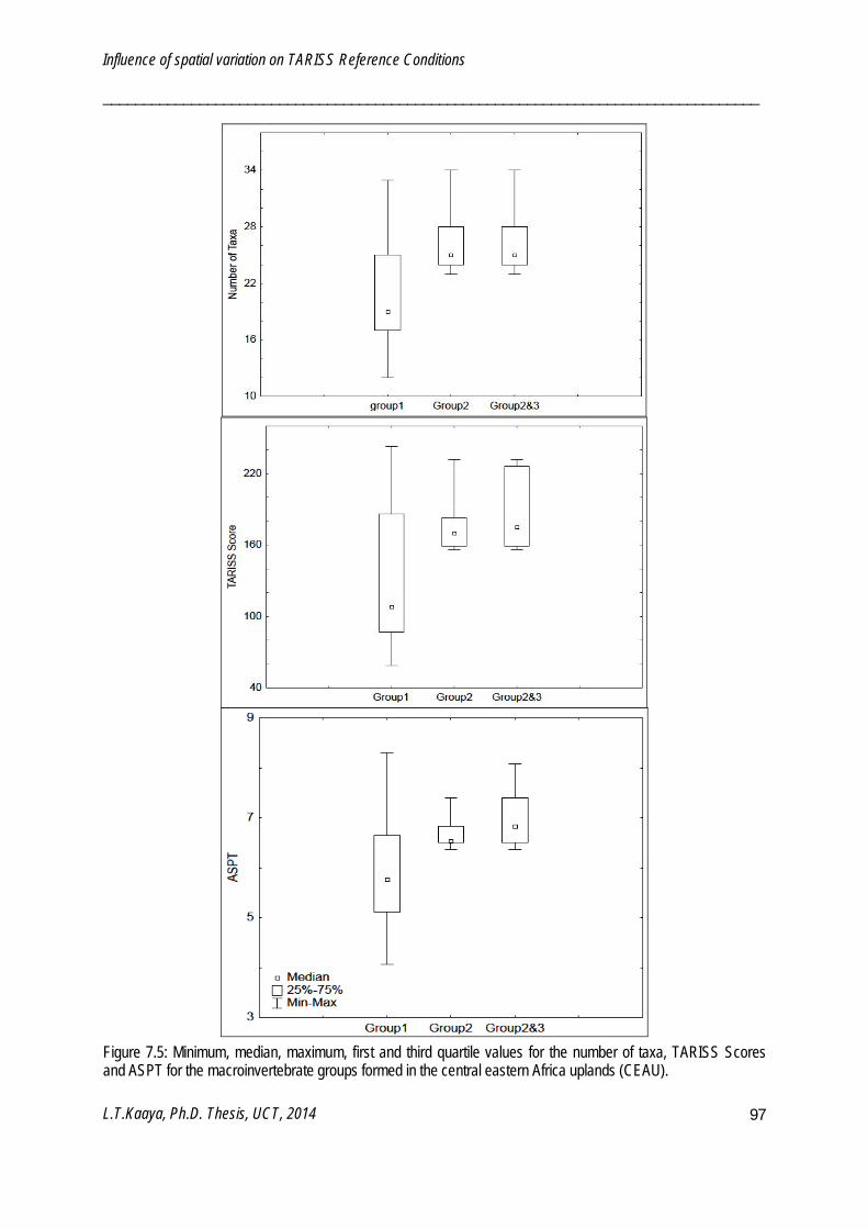
Influence of spatial variation on TARISS Reference Conditions
__________________________________________________________________________________
L.T.Kaaya, Ph.D. Thesis, UCT, 2014
97
Figure 7.5: Minimum, median, maximum, first and third quartile values for the number of taxa, TARISS Scores and ASPT for the macroinvertebrate groups formed in the central eastern Africa uplands (CEAU).

Influence of spatial variation on TARISS Reference Conditions
__________________________________________________________________________________
L.T.Kaaya, Ph.D. Thesis, UCT, 2014
98
Figure 7.6: Minimum, median, maximum, first and third quartile values for the number of taxa, TARISS Scores and ASPT for the macroinvertebrate groups formed in the central eastern Africa lowlands (CEAL).
Influence of spatial variation on TARISS Reference Conditions
__________________________________________________________________________________
L.T.Kaaya, Ph.D. Thesis, UCT, 2014
99
Environmental variables
Environmental variables were ranked based on their discriminatory power following Partial Wilk’s Lambda (lower numbers indicate higher discriminating power) as shown previously in Table 7.2. Electrical conductivity, water temperature, altitude and active channel width were identified as discriminating variables in PHU. Results showed that discrimination was more significant and clearer in group three (means of canonical correlations = 6.74369) than with group one (means of canonical correlations = -1.99) and group two (means of canonical correlations = 0.15233). The discrimination function shows that a site with higher water temperatures, wider active channel, lower electrical conductivity and altitude is less likely to be in group three and more likely to be in group one.
In CEAU, active channel width, percentage sand, latitude, percentage cobble, percentage boulder, and nitrate concentration were the best discriminating environmental variables. The discrimination was more significant and clearer in group two (means of canonical correlations = -3.4279) than group three (means of canonical correlations = 2.1628) and group one (means of canonical correlations = 0.9153). Discrimination results showed that, with narrower active channel, lower percentage of sand, higher latitudes, higher percentages of cobble and boulder, and higher nitrate concentrations, a site is more likely to be in group two and less likely to be in group three and one. Latitude and Longitude were identified as important discriminating environmental variables in CEAL. The discriminating variables appear to be more significant and clearer in separating group two (means of canonical correlations = 53.7812) than group one (means of canonical correlations = -11.9514). DFA results indicate that a site with lower latitude and longitudes is more likely to be a member of group two and less likely a member of group one.
In summary all four categories of variables, namely catchment, water chemistry, site and habitat, were important in discriminating among the faunal groups among river types as shown in Table 7.3. Physico-chemical variables and site characteristic was important only in PHU. Catchment characteristics showed a vital discriminating role in all river types where altitude was important in PHU, latitude in CEAU and latitude and longitude in CEAL. Latitude was the most discriminating variable in CEAL, percentage boulder in CEAU and water temperature in PHU.

Influence of spatial variation on TARISS Reference Conditions
__________________________________________________________________________________
L.T.Kaaya, Ph.D. Thesis, UCT, 2014
100
Table 7.3: Environmental variables that best discriminated groups of sites based on macroinvertebrates assemblages in Pangani highland uplands (PHU), central eastern Africa uplands (CEAU) and central eastern Africa lowlands (CEAL). (DP = Discriminatory Power, PWL = Partial Wilki’s Lambda, FS = Factor structure). Variable Category
Variable PHU CEAU CEAL
DP PWL FS DP PWL FS DP PWL FS n 13 20 14
Catchment Latitude 3 0.683 -0.450 1 0.013 -0.849 Longitude 2 0.722 -0.110 Altitude 3 0.551 0.230
Physico-chemistry
Conductivity 2 0.373 0.443 Water temperature
1 0.189 -0.225
Nitrate 6 0.832 -0.144 Site Active channel
width 4 0.701 -0.195 1 0.597 0.126
Habitat % Boulder 5 0.759 -0.758 % Cobble 4 0.706 -0.385 % Sand 2 0.651 0.415
Establishment of TARISS Reference conditions
Grouping of reference sites based on macroinvertebrate occurrence within river types (Figure 7.4-7.6) gave an opportunity for developing biological meaningful reference conditions. Groups that had at least five sites were used for development of reference conditions. In PHU, Group 1 and combined Groups 2 and 3 were considered for development of reference conditions. In CEAU, Group 1 was highly variable in all TARISS metrics. Ranges for TARISS metrics were 12 to 33 for number of taxa, 59 to 243 for TARISS Scores and 4.1 to 8.3 for ASPT. Such vast variation in metrics is considered unsuitable for development of reference conditions. Three sites namely R05, R06 and U10 had TARISS metrics higher than other sites in the group (191 to 220 TARISS score and 7.1 to 8.3 ASPT) which contributed to the high ranges. An alternative approach of delineating the river type based on latitude and substrate composition was used given that three substrate percentages; ‘boulder, cobble and sand’ were among the best discriminating variables in CEAU. Latitude and substrate percentages divided CEAU into two groups; Group 1 comprising sites occurring at latitudes >10oS and composed of mixed of substrates; and Group 2 which has sites that occur at latitudes ≤10oS and do not have boulders or cobble and is dominated by sand and silt substrates. In CEAL, Group 2 had only two sites which when combined with Group 1, the variability in TARISS metrics increased; as a result, only Group 1 was considered for the development of reference conditions.
Influence of spatial variation on TARISS Reference Conditions
__________________________________________________________________________________
L.T.Kaaya, Ph.D. Thesis, UCT, 2014
101
Linear regression analysis showed significant positive relationship between the number of sampled biotopes and the number of taxa (r=0.4081, p=0.006) and TARISS scores (r=0.3365, p=0.0096) (Figure 7.7). ASPT, also showed a positive, however not significant correlation with the number of sampled biotopes (r=0.1714 p=0.2659) (Figure 7.7). These results suggest that ASPT is less affected by the number of biotopes sampled at a site, such that at a site with one biotope; number of taxa and TARISS scores are more likely to be lower than expected while the ASPT value will be less affected and more likely be close to the expected value. Based on these relationships, it is recommended to have an interpretation guideline that incorporates ASPT and either number of taxa or TARISS scores. An example of such interpretation guideline is for the South African Scoring System which uses both ASPT and SASS Scores to delineate biological bands representing different ecological status (Dallas 2007a, Dallas and Day 2007). In this study, the same approach was used to develop TARISS interpretation guidelines in form of biological bands developed using ASPT and TARISS scores.
Reference conditions for the five groups in all river types were developed and their expected ranges are provided in Table 7.4. The reference condition ranges include the physico-chemical and biological conditions that were measured and calculated from the sites during this study. Two groups namely combined Group 2and 3 in PHU and Group 2 in CEAU did not have impaired test sites to enable validation of the reference conditions, thus only preliminary reference conditions were provided for these two groups. The remaining three groups namely Group 1 in PHU, Group 1 in CEAU and Group 1 in CEAL were validated using biological conditions as TARISS scores and ASPT from impaired or test sites. Biological bands for Group 1 in PHU, Group 1 in CEAU and Group 1 in CEAL were thus derived.
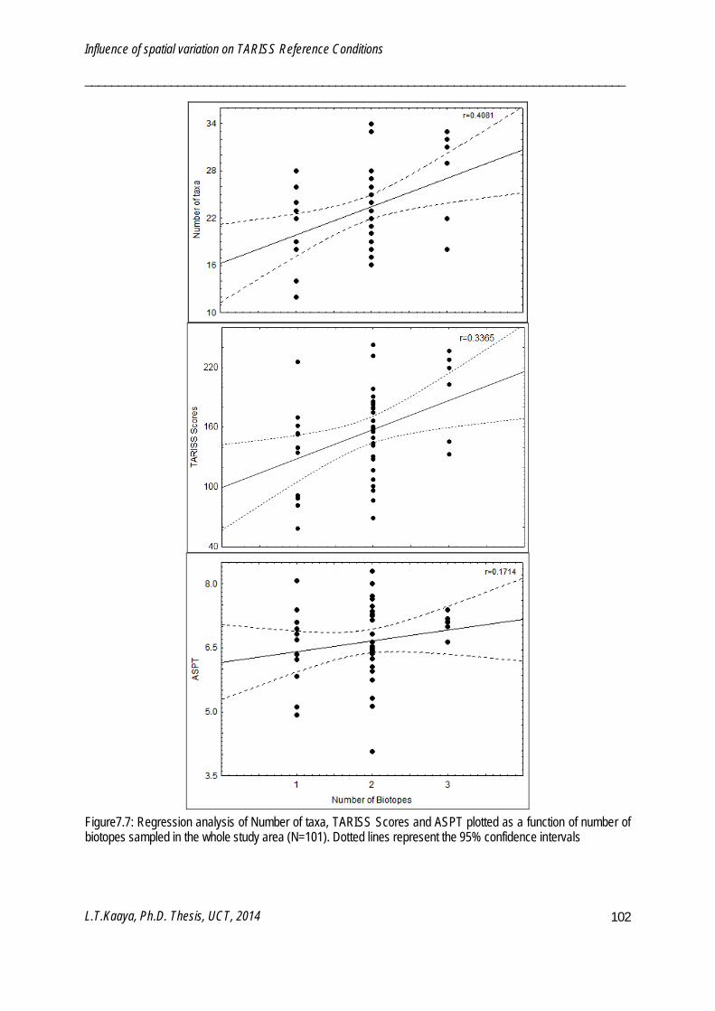
Influence of spatial variation on TARISS Reference Conditions
__________________________________________________________________________________
L.T.Kaaya, Ph.D. Thesis, UCT, 2014
102
Figure7.7: Regression analysis of Number of taxa, TARISS Scores and ASPT plotted as a function of number of biotopes sampled in the whole study area (N=101). Dotted lines represent the 95% confidence intervals
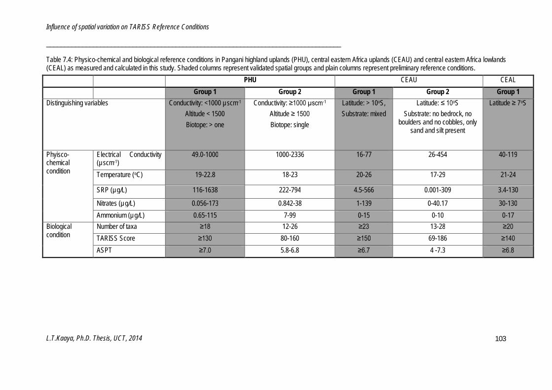
Influence of spatial variation on TARISS Reference Conditions
__________________________________________________________________________________
L.T.Kaaya, Ph.D. Thesis, UCT, 2014
103
Table 7.4: Physico-chemical and biological reference conditions in Pangani highland uplands (PHU), central eastern Africa uplands (CEAU) and central eastern Africa lowlands (CEAL) as measured and calculated in this study. Shaded columns represent validated spatial groups and plain columns represent preliminary reference conditions. PHU CEAU CEAL Group 1 Group 2 Group 1 Group 2 Group 1 Distinguishing variables Conductivity: <1000 µscm-1
Altitude < 1500 Biotope: > one
Conductivity: ≥1000 µscm-1 Altitude ≥ 1500 Biotope: single
Latitude: > 10oS, Substrate: mixed
Latitude: ≤ 10oS Substrate: no bedrock, no
boulders and no cobbles, only sand and silt present
Latitude ≥ 7oS
Phyisco-chemical condition
Electrical Conductivity (µscm-1)
49.0-1000 1000-2336 16-77 26-454 40-119
Temperature (oC) 19-22.8 18-23 20-26 17-29 21-24
SRP (µg/L) 116-1638 222-794 4.5-566 0.001-309 3.4-130
Nitrates (µg/L) 0.056-173 0.842-38 1-139 0-40.17 30-130 Ammonium (µg/L) 0.65-115 7-99 0-15 0-10 0-17
Biological condition
Number of taxa ≥18 12-26 ≥23 13-28 ≥20 TARISS Score ≥130 80-160 ≥150 69-186 ≥140 ASPT ≥7.0 5.8-6.8 ≥6.7 4 -7.3 ≥6.8

Influence of spatial variation on TARISS Reference Conditions
__________________________________________________________________________________
L.T.Kaaya, Ph.D. Thesis, UCT, 2013 104
Derivation and validation of biological bands
Test sites and reference sites were used together to develop and validate biological bands.Review of previous developed biological bands in South African studies provided a baseline of percintiles that can be used to classify the distribution of TARISS metrics into different ecological categories. Data in this study were also explored at various percentiles to establish suitable percentiles for use in each river type. 90th, 67.5th, 45th and 22.5th percentiles of TARISS scores and ASPTs were used as boundaries of biological bands. The 67.5th percentile was considered as a boundary between reference and impaired conditions. In Group 1 in PHU, the 67.5th percentile with TARISS Score of 84 and ASPT of 6.4, could not differentiate the reference sites from test sites thus the scale was increased and the 85th percentile with TARISS Score of 120 and ASPT of 7.1 was used to define the boundary between reference and impaired conditions. Percentiles for biological bands in PHU were 85th, 56.7th and 28.3th. Therefore, in PHU there was no biological band X which was supposed to indicate a more than reference condition ecological status (Figure 7.8).
Figure 7.8: Scatter plot of ASPT values as a function of TARISS Scores from reference and test sites in Group 1 in PHU. Biological bands calculated by percentiles are shown by the solid lines and labeled X, A, B, C, and D. Black symbols represent reference sites while transparent symbols represent monitoring sites.
In Group 1 in CEAU, at the 67.5th percentile boundary had TARISS score = 157 and ASPT = 6.7 which separated reference conditions from impaired conditions as shown in Figure 7.9. Three test sites, R07, R09 and W09, fell in band B of reference sites possibly because they had few taxa summing into low scores hence resulting to higher ASPT values. In Group 1 in CEAL, reference sites were separated from test sites except for site U05 which fell in band B of test sites (Figure 7.6). Although the reason for U05 to fall in the test band B could be an artefact of sampling error, but this site differed from other reference sites by not having a stone biotope and characterised only by GSM and vegetation biotopes which might have contributed to its lower score and ASPT. The 67.5th percentile boundary had TARISS score = 142 and ASPT = 6.9 as shown in Figure 7.10.

Influence of spatial variation on TARISS Reference Conditions
__________________________________________________________________________________
L.T.Kaaya, Ph.D. Thesis, UCT, 2013 105
Figure 7.9: Scatter plot of ASPT values as a function of TARISS Scores from reference and test sites in Group 1 in CEAU. Biological bands calculated by percentiles are shown by the solid lines and labeled X, A, B, C, and D. Black symbols represent reference sites while transparent symbols represent monitoring sites.
Figure 7.10: Scatter plot of ASPT values as a function of TARISS Scores from reference and test sites in Group 1 in CEAL. Biological bands calculated by percentiles are shown by the solid lines and labeled X, A, B, C, and D. Black symbols represent reference sites while transparent symbols represent monitoring sites.
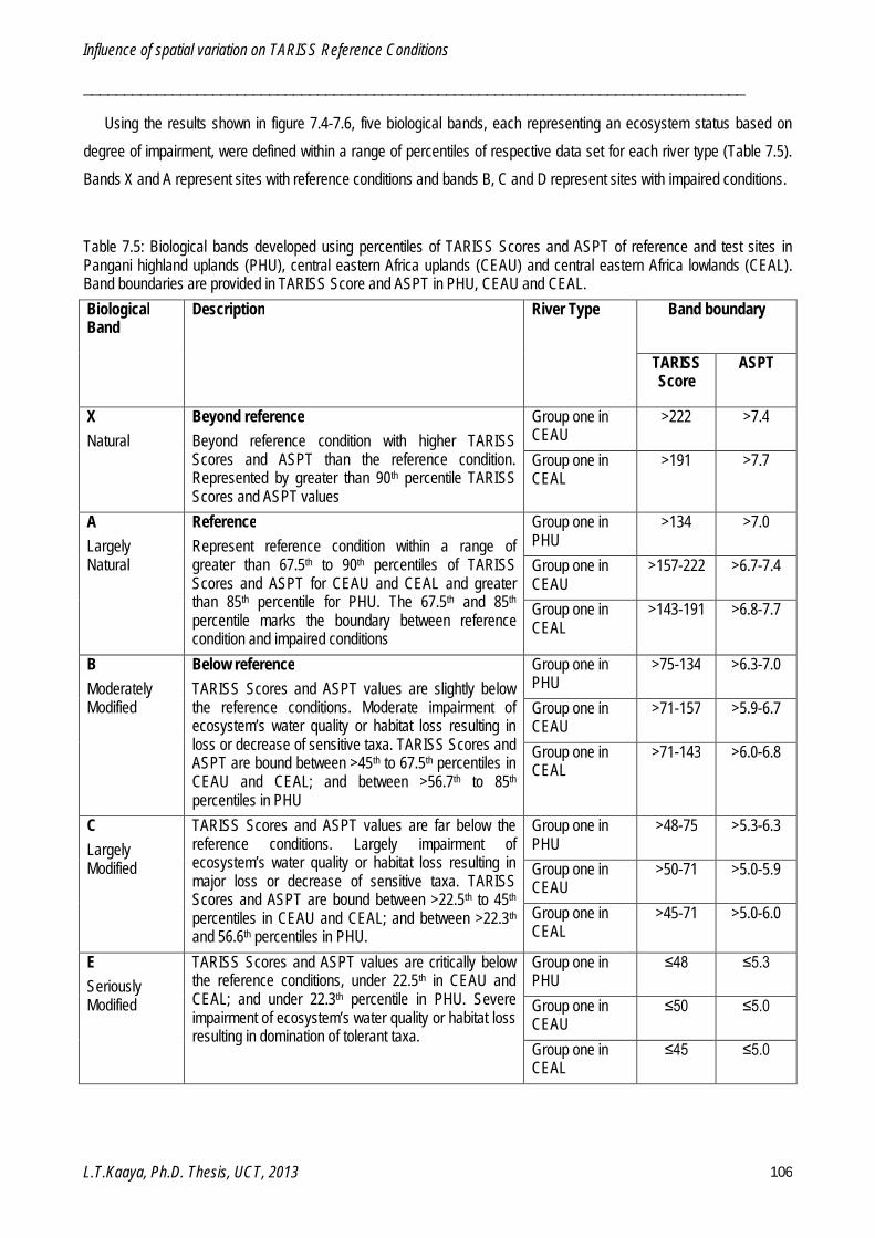
Influence of spatial variation on TARISS Reference Conditions
__________________________________________________________________________________
L.T.Kaaya, Ph.D. Thesis, UCT, 2013 106
Using the results shown in figure 7.4-7.6, five biological bands, each representing an ecosystem status based on degree of impairment, were defined within a range of percentiles of respective data set for each river type (Table 7.5). Bands X and A represent sites with reference conditions and bands B, C and D represent sites with impaired conditions.
Table 7.5: Biological bands developed using percentiles of TARISS Scores and ASPT of reference and test sites in Pangani highland uplands (PHU), central eastern Africa uplands (CEAU) and central eastern Africa lowlands (CEAL). Band boundaries are provided in TARISS Score and ASPT in PHU, CEAU and CEAL. Biological Band
Description River Type Band boundary
TARISS Score
ASPT
X Natural
Beyond reference Beyond reference condition with higher TARISS Scores and ASPT than the reference condition. Represented by greater than 90th percentile TARISS Scores and ASPT values
Group one in CEAU
>222 >7.4
Group one in CEAL
>191 >7.7
A Largely Natural
Reference Represent reference condition within a range of greater than 67.5th to 90th percentiles of TARISS Scores and ASPT for CEAU and CEAL and greater than 85th percentile for PHU. The 67.5th and 85th percentile marks the boundary between reference condition and impaired conditions
Group one in PHU
>134 >7.0
Group one in CEAU
>157-222 >6.7-7.4
Group one in CEAL
>143-191 >6.8-7.7
B Moderately Modified
Below reference TARISS Scores and ASPT values are slightly below the reference conditions. Moderate impairment of ecosystem’s water quality or habitat loss resulting in loss or decrease of sensitive taxa. TARISS Scores and ASPT are bound between >45th to 67.5th percentiles in CEAU and CEAL; and between >56.7th to 85th percentiles in PHU
Group one in PHU
>75-134 >6.3-7.0
Group one in CEAU
>71-157 >5.9-6.7
Group one in CEAL
>71-143 >6.0-6.8
C Largely Modified
TARISS Scores and ASPT values are far below the reference conditions. Largely impairment of ecosystem’s water quality or habitat loss resulting in major loss or decrease of sensitive taxa. TARISS Scores and ASPT are bound between >22.5th to 45th percentiles in CEAU and CEAL; and between >22.3th and 56.6th percentiles in PHU.
Group one in PHU
>48-75 >5.3-6.3
Group one in CEAU
>50-71 >5.0-5.9
Group one in CEAL
>45-71 >5.0-6.0
E Seriously Modified
TARISS Scores and ASPT values are critically below the reference conditions, under 22.5th in CEAU and CEAL; and under 22.3th percentile in PHU. Severe impairment of ecosystem’s water quality or habitat loss resulting in domination of tolerant taxa.
Group one in PHU
≤48 ≤5.3
Group one in CEAU
≤50 ≤5.0
Group one in CEAL
≤45 ≤5.0

Influence of spatial variation on TARISS Reference Conditions
__________________________________________________________________________________
L.T.Kaaya, Ph.D. Thesis, UCT, 2013 107
Discussion
Understanding natural variability of river systems and their macroinvertebrate assemblages at different spatial scales in a particular region is important for the interpretation of bioassessment data and making reliable inferences. Inherent variability in macroinvertebrate assemblages among sites in a region may influence the establishment of reference conditions because reference conditions are usually defined from a group of similar sites. One way of dealing with natural variability is classifying rivers into homogenous groups under the principle that homogenous river types will have homogenous biotic assemblages. However this is not always the case and macroinvertebrate assemblages within homogenous rivers may still vary because of other factors such as predation (Crowl et al. 1997), evolutionary aspects (Dallas 2002) and biotope availability and quality (Kay et al. 1999, Dallas 2004a).
Investigation of spatial variability of macroinvertebrate assemblages in this study showed that assemblages do vary within all three homogenous river types examined namely PHU, CEAU and CEAL. Closer examination of macroinvertebrate assemblages within each river type indicated that, the grouping in PHU was influenced by catchment, physico-chemical and site characteristics. Water temperature was the most significant discriminating variable in PHU, possibly influenced by altitude. Differences in altitude may drive local longitudinal climatic differences, which in turn influence differences in macroinvertebrate assemblages. Electrical conductivity was the second discriminator and may reflect geological and hydro-geochemical characteristics of the region. Sites in Group 3 in PHU originate from the south-eastern side of Mount Meru, which is dominated by volcanic rocks contributing to highly alkaline water chemistry with high conductivity.
In CEAU, environmental variables grouped sites into narrower streams with higher percentage of boulders and cobble at latitudes higher than 10oS (Group 2) and wider streams dominated by sandy and silt substrate occurring at latitudes equal and lower than10oS (Group 1) except for R05 and R05 sites. The grouping also reflects catchment differences as Group 1 sites with exception of R05 and R06, originated from the Luwegu catchment and sites in Group 2 are from the Wami and Ruvu catchments. The variability in substrate type in CEAU influenced habitat characteristics which support different types and forms of food for the biota (Buss et al. 2004) and this could also contribute to the variation in macroinvertebrate assemblages. Variation in substrate type and composition influenced TARISS metrics. TARISS scores and ASPT values varied between sandy and stone biotopes; and also varied within the stone rivers. Sites from mountain streams dominated by large stones (i.e. bedrock and boulders) had lower TARISS scores and ASPT values compared to upper foothill sites dominated by gravels and cobbles. Studies have shown that macroinvertebrate abundance and taxon richness increase with size of substrates up to gravel and cobble (Minshall 1984, Mackay 1992). This was true even with number of taxa, which was generally higher at sites with higher percentage of gravel and cobble than in sites with more sand, boulders and bedrock. Nitrate concentration was also a discriminator variable in CEAU where sites in Group 1 had lower nitrate concentrations of ≤0.04mg/L; nitrate concentration in Group 2 sites ranged from 0.0167-0.0834mg/L; and in Group 3, site R04 had the highest nitrate concentration of 0.1394mg/L. The variation in nitrate concentrations may be caused by climatic features such as rainfall and weathering of rocks and soil; and by catchment characteristics such as geology and landform (Dallas and Day 2004).
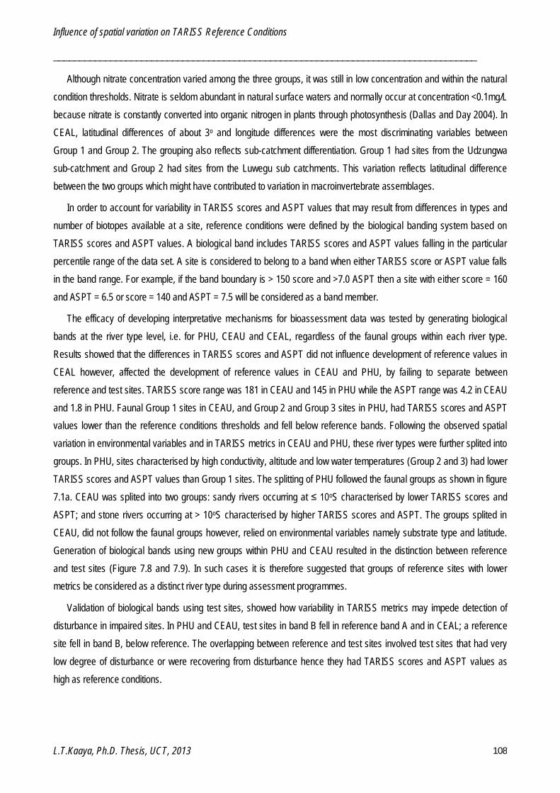
Influence of spatial variation on TARISS Reference Conditions
__________________________________________________________________________________
L.T.Kaaya, Ph.D. Thesis, UCT, 2013 108
Although nitrate concentration varied among the three groups, it was still in low concentration and within the natural condition thresholds. Nitrate is seldom abundant in natural surface waters and normally occur at concentration <0.1mg/L because nitrate is constantly converted into organic nitrogen in plants through photosynthesis (Dallas and Day 2004). In CEAL, latitudinal differences of about 3o and longitude differences were the most discriminating variables between Group 1 and Group 2. The grouping also reflects sub-catchment differentiation. Group 1 had sites from the Udzungwa sub-catchment and Group 2 had sites from the Luwegu sub catchments. This variation reflects latitudinal difference between the two groups which might have contributed to variation in macroinvertebrate assemblages.
In order to account for variability in TARISS scores and ASPT values that may result from differences in types and number of biotopes available at a site, reference conditions were defined by the biological banding system based on TARISS scores and ASPT values. A biological band includes TARISS scores and ASPT values falling in the particular percentile range of the data set. A site is considered to belong to a band when either TARISS score or ASPT value falls in the band range. For example, if the band boundary is > 150 score and >7.0 ASPT then a site with either score = 160 and ASPT = 6.5 or score = 140 and ASPT = 7.5 will be considered as a band member.
The efficacy of developing interpretative mechanisms for bioassessment data was tested by generating biological bands at the river type level, i.e. for PHU, CEAU and CEAL, regardless of the faunal groups within each river type. Results showed that the differences in TARISS scores and ASPT did not influence development of reference values in CEAL however, affected the development of reference values in CEAU and PHU, by failing to separate between reference and test sites. TARISS score range was 181 in CEAU and 145 in PHU while the ASPT range was 4.2 in CEAU and 1.8 in PHU. Faunal Group 1 sites in CEAU, and Group 2 and Group 3 sites in PHU, had TARISS scores and ASPT values lower than the reference conditions thresholds and fell below reference bands. Following the observed spatial variation in environmental variables and in TARISS metrics in CEAU and PHU, these river types were further splited into groups. In PHU, sites characterised by high conductivity, altitude and low water temperatures (Group 2 and 3) had lower TARISS scores and ASPT values than Group 1 sites. The splitting of PHU followed the faunal groups as shown in figure 7.1a. CEAU was splited into two groups: sandy rivers occurring at ≤ 10oS characterised by lower TARISS scores and ASPT; and stone rivers occurring at > 10oS characterised by higher TARISS scores and ASPT. The groups splited in CEAU, did not follow the faunal groups however, relied on environmental variables namely substrate type and latitude. Generation of biological bands using new groups within PHU and CEAU resulted in the distinction between reference and test sites (Figure 7.8 and 7.9). In such cases it is therefore suggested that groups of reference sites with lower metrics be considered as a distinct river type during assessment programmes.
Validation of biological bands using test sites, showed how variability in TARISS metrics may impede detection of disturbance in impaired sites. In PHU and CEAU, test sites in band B fell in reference band A and in CEAL; a reference site fell in band B, below reference. The overlapping between reference and test sites involved test sites that had very low degree of disturbance or were recovering from disturbance hence they had TARISS scores and ASPT values as high as reference conditions.
Influence of spatial variation on TARISS Reference Conditions
__________________________________________________________________________________
L.T.Kaaya, Ph.D. Thesis, UCT, 2013 109
In such situations, it is recommended that interpretation of TARISS data requires investigation of the ecological conditions at a site as well as identifying biological bands, in order to avoid misclassifying reference sites as impaired or test sites as reference. Reference sites did not always have highest TARISS scores and ASPT values in a particular river type such as sites in the sandy rivers in CEAU and sites in Group 2 and 3 in PHU. In Group 1 of PHU; the 67.5th percentile was inadequate to separate reference sites from disturbed sites.
Most of the reference sites in PHU can be considered as the best available in the region and have the potential to go below reference if management interventions are not applied. Therefore, for the practicality of distinguishing reference conditions from below reference conditions, TARISS score and ASPT boundaries were increased from 67.5th to 85th percentile.
In conclusion, variation of macroinvertebrate assemblages observed in all three river types was driven by both catchment and local variables. Macroinvertebrate variation was translated into TARISS scores and ASPT values to the extent of influencing development of reference conditions in PHU and CEAU river types. For river types exhibiting significant natural variability, it is necessary to further delineate a particular river type in order to obtain reliable reference conditions capable of detecting disturbance in test tests. Thus, it is important to understand spatial variability in TARISS metrics in relation to inherent variation in environmental variables for each river type in order to increase the accuracy and reliability of TARISS conclusions.
Synthesis and General Discussion
__________________________________________________________________________________
L.T.Kaaya, Ph.D. Thesis, UCT, 2013 110
Chapter 8: Synthesis and General Discussion
________________________________________________________________

Synthesis and General Discussion
__________________________________________________________________________________
L.T.Kaaya, Ph.D. Thesis, UCT, 2013 111
Introduction
This thesis focused on disclosing the potentials and opportunities for bioassessment of river systems in Tanzania. Important concepts such as regional classification of rivers, spatio-temporal variability of macroinvertebrates and reference conditions approach have been examined and discussed in the context of bioassessment. Tanzania River Scoring System (TARISS), macroinvertebrates-based bioassessment method was developed and validated. Analyses and discussions through chapters 3 to 7 revealed several aspects regarding TARISS application such as the influence of spatial and temporal variation of macroinvertebrate assemblages and how they may influence the establishment of TARISS reference conditions and the interpretation. In this synthesis chapter, such issues are further discussed, major findings are summarised and way forward is proposed for bioassessment of rivers in Tanzania.
Does river type classification minimize the effect of natural spatial variation in macroinvertebrate assemblages on bioassessment?
Classification of rivers into types is considered a way to help account for natural spatial variation in biotic assemblages in bioassessment methods under the hypothesis that, ‘rivers with similar abiotic features have similar biotic assemblages’ (Brown et al. 1996, Hawkins et al. 2000, Sandin and Verdonschot 2006 and Turak and Koop 2008). The validity of this hypothesis is influenced by the level at which the homogeneity rivers in abiotic features is considered. Similarities in macroinvertebrate assemblages in river types formed under ecoregion-landform classification were higher than in river types formed under the ecoregion classification (Chapter 4). River types formed at the ecoregion-slope class classification showed significant within-type differences in macroinvertebrate assemblages and TARISS metrics resulting in two sub-Groups in each river type. The sub-Groups were differentiated by either catchment or local abiotic factors related to climate, geology, geomorphologic landform, channel form and habitat substrate. Thus the hypothesis is more likely to be true with lower (reach) classification level than higher (basin) classification levels. Lower or reach level classification gives stronger partitioning of macroinvertebrate assemblages and may have higher power for detecting difference and changes in biological assemblages. Lower classification levels give large numbers of river types however, and it may become impractical to provide sufficient reference sites, and expensive to implement (Mykra et al. 2009). Although the choice of which regional classification should be adopted is expected to be determined by programme objectives, management goals and financial resources, care should be taken not to compromise the degree of the biological homogeneity. Within a spatial region, where natural variation in abiotic features is inevitable, classifying rivers into types provides an organized partitioning framework in biotic assemblages which minimizes the effect of natural biotic variability and gives clarity in bioassessment.

Synthesis and General Discussion
__________________________________________________________________________________
L.T.Kaaya, Ph.D. Thesis, UCT, 2013 112
The effect of biotope availability at a site on TARISS metrics and interpretation
Not all sites occurring in a river type are expected to have all three TARISS biotopes available. Biotope availability at a site and biotope variability among sites occurring in the same river type may influence macroinvertebrate assemblages and TARISS metrics and may lead to erroneous comparisons between reference and test sites. Interpretation of data among sites sampled from different biotopes may be difficult. Several options for dealing with this problem have been put forward. They include interpreting data on a site basis despite biotope variability; limiting sampling to one biotope type (Parsons and Norris 1996; Hewlett 2000); comparing biotope data separately among sites (Chessman 1995 and Kay et al. 1999) and limiting sampling to two key biotopes in a region (Dallas 2007a). Limiting sampling to one or two biotopes is impractical for Tanzanian rivers, which are diverse, making it unlikely to find same biotope or pair of biotope present in all test and reference sites. All three TARISS biotopes occur in Tanzanian rivers and each can occur as a dominant biotope in different sites and be absent from others. Investigation of the influence of number of sampled biotopes at a site and TARISS metrics showed that number of taxa and TARISS score have stronger and more significantly positive correlations with number of sampled biotopes than with ASPT. Since differences in number of sampled biotopes influence number of taxa and TARISS scores than ASPT it is recommended to interpret and derive conclusions based on either number of taxa or TARISS score and ASPT value simultaneously because the ASPT value will less likely be influenced and more likely be close to the expected value. This theory lent support to the TARISS interpretation concept of biological bands (Chapter 7), which was adopted from the South African approach (Dallas and Day 2007). This concept involves development and use of biological bands defined by ranges of TARISS scores and ASPT values which ensure incorporation of biotope variability in the interpretation of TARISS data.
Does temporal variation in macroinvertebrates influence reference conditions?
Influences of temporal variation on bioassessment are discussed in Chapter 6, where it was revealed that temporal variation in macroinvertebrate taxa occurred in all river types while temporal variation in assemblages occurred only in CEAL. Number of taxa, TARISS scores and ASPT values varied between wet and dry periods only in the CEAL stone biotope data set. Therefore the influence of temporal variation should be considered important only in regions were temporal variability in macroinvertebrates has been ascertained, meaning that prior to bioassessment using TARISS, temporal variability in macroinvertebrates must be examined. In regions where temporal variation is minimal, it is not necessary to restrict the establishment of reference conditions to a single season. But for regions such as CEAL, were temporal variation is significant, actions for reducing the effects of temporal variation in reference conditions must be put in place. Approaches for incorporating seasonal variability include collection of samples within a short period of time (e.g in Barbour et al. 1999) and combining multiple-season samples for each site (e.g in Wright 2000). Combined-seasons datasets for Tanzania increased the accuracy of prediction of biotic composition of test sites, as had previously been found by Furse et al. (1984). Thus for TARISS, two options are recommended: firstly the development and use of seasonal reference conditions for testing sites (i.e. wet reference conditions should be used to test sites in the wet season). Secondly, development and use of combined-seasons reference conditions for testing sites from either of the
Synthesis and General Discussion
__________________________________________________________________________________
L.T.Kaaya, Ph.D. Thesis, UCT, 2013 113
seasons. In the use of combined reference condition, all seasonally associated differences must be considered in the interpretation. For example absence of taxa known to occur only or more frequently in a particular season, should be known to reflect seasonality and not disturbance.
Potentials, Challenges and Way forward for TARISS as a bioassessment method for Tanzanian rivers.
With the increasing popularity, efficiency and usefulness of bioassessment methods in assessment and monitoring programmes for rivers globally (Wright et al. 1984, Rosenberg et al. 1999, Chutter 1998, Barbour et al. 1999 and Dickens and Graham 2002), Tanzania has also shown the need to use biological assessment methods. Endeavors have been conducted in Tanzanian river basins using bioassessment methods developed for other regions. For instance SASS, the South African method, has been used in the Pangani basin (PWBO/IUCN 2007) and the Mara basin (EFA-Mara river basin 2007). The long-term vision of my study is for Tanzania to have a national biotic index for assessment of rivers. In this study, a bioassessment method for assessment and monitoring anthropogenic disturbance in Tanzanian rivers, was developed and validated in three river types from two ecoregions. The way forward towards the national biotic index thus requires further validation of TARISS in additional ecoregions. Although TARISS was validated in the two ecoregions, it can be used with confidence in other ecoregions across the country and is expected to detect disturbance and change in rivers, given that the sampling and analytical procedures remain the same. Experiences and challenges that may be encountered with use of TARISS in additional ecoregions will facilitate the modification and validation processes of TARISS. For example when new macroinvertebrate taxa are identified, they will be incorporated in the TARISS method. Guidelines for interpreting TARISS such as reference conditions and reference taxa may be different among ecoregions. Therefore it is necessary to establish reference conditions for the additional ecoregions in the country in order to facilitate interpretation of TARISS data. Procedures for establishing reference conditions are detailed in Chapter 7, and illustrated in Figure 8.1 in order to assist researchers, TARISS practitioners and water-basin officers.
TARISS is suitable for assessment and monitoring of river’s water quality and ecosystem status in general. In monitoring programmes, TARISS can be used to assess spatial and temporal trends of ecosystem state and to assess emerging and potential impacts of infrastructure, industrial and agricultural developments. Given that TARISS uses a reference-condition approach to compare test sites, it is important to tally the monitoring objectives with the type of reference condition to be used. Reference conditions as a representation of least-impacted sites organised by physical, chemical and biological variables (Reynoldson et al. 1997), enable the detection of deviation of rivers from natural conditions due to anthropogenic disturbance.
There are two categories of reference conditions, namely site-specific and region-specific. Site-specific reference conditions either 1) compare the same site over a period of time or 2) compare between two sites either upstream or downstream a disturbance or 3) in a paired scenario, compare between a test site and a reference site. Region-specific or type-specific reference conditions are derived from a group of similar reference sites.

Synthesis and General Discussion
__________________________________________________________________________________
L.T.Kaaya, Ph.D. Thesis, UCT, 2013 114
Region-specific reference conditions may be developed at the level of ecoregion, slope class, landform or river type and biological attributes of a group of reference sites in a particular level are compared to a test site occurring in the same spatial group. In this study, regional reference conditions were established at an ecoregion-slope class level and validated using biotic data from test sites for the PHU, CEAU and CEAL. Of the three TARISS metrics, TARISS score and ASPT were more robust than number of taxa in detecting changes using region-specific reference conditions. The number of taxa is considered a suitable metric in detecting changes using site-specific reference conditions, though. Importantly, reference conditions should be used with background knowledge of the spatial and temporal variation in macroinvertebrate assemblages in the particular river type or site.
Although the reference condition approach provides a useful measure of anthropogenic disturbance, there are possibilities of reference-condition sites are not being distinguishable from test sites. TARISS metrics did not necessarily differentiate reference from test sites, possibly because of the natural spatial variation among sites. The biological banding system developed using regional reference conditions as a guideline for interpreting TARISS was capable of differentiating test sites from reference conditions in most cases. Few sites were misclassified as either a reference site instead of test site or a test site instead of reference site however. Examination of mis-classified sites indicated that they were either influenced by an anthropogenic disturbance such as dam construction (R01) or flower plantation (P28) or had been restored from disturbance (P13). For such sites, it is recommended that intra-site monitoring using site-specific reference condition over time should be used in order to monitor changes and establish the ecological status of the particular site. Changes over time might be essential in sites occurring in close proximity to the reference band (67.5th to 90th percentile) such as sites that are on transition from recovery to impairment and vice versa. Note that, a reference biological band i.e. 67.5th to 90th percentile, is a range and will most likely have certain TARISS score and ASPT values slightly above or lower the reference band. Furthermore, interpretation of TARISS data should be done together with analysis of environmental variables, which should increase the robustness of the conclusions about ecological status.
The sensitivity weightings of the majority of TARISS taxa reflect without doubt the ecosystem condition of river sites where they occur in relation to anthropogenic disturbance. Sensitivity weightings of a few taxa are controversial, however. The Chironomidae, is considered to be tolerant and thus has been assigned a low sensitivity weighting (2) but in fact varies widely in sensitivity to disturbance at sub-family, generic and specific level.
Although the TARISS taxon list does not go to generic and specific level, an understanding of lower taxonomic levels of the Chironomidae ,their distribution in Tanzanian rivers and their sensitivity to anthropogenic disturbance, would be valuable particularly where a sensitive genus or species occurring in a reference site in influences the overall TARISS score and ASPT value. Furthermore, investigation of the frequency of occurrence of taxa at reference sites in this study, has also shown that the Potamonautidae, which have been assigned a low sensitivity weighting (3), occur in higher frequencies in reference sites than disturbed sites. Therefore, studies on
Synthesis and General Discussion
__________________________________________________________________________________
L.T.Kaaya, Ph.D. Thesis, UCT, 2013 115
taxonomy, sensitivity to disturbance and distribution of the Chironomidae and Potamonautidae in Tanzanian rivers are recommended.
Examination of occurrence and distribution of taxa between reference and disturbed sites suggested that certain macroinvertebrate orders can stand out and be used to detect disturbance in rivers. These are the Ephemeroptera, Diptera, Odonata and Trichoptera. Sensitivity weightings ranges of the Ephemeroptera and Trichoptera ranges from moderately to highly sensitive (6-15); and of the Diptera and Odonata from least to moderately sensitive (1-10). The Diptera have more least-sensitive taxa than the Odonata, and the Ephemeroptera have more highly sensitive taxa than the Trichoptera do. Number of taxa within the orders varied with Trichoptera having fewer taxa (6) than Odonata (9), Ephemeroptera (10) and Diptera (10). Based on these observations, I recommend further investigations on the potential of developing a biotic index based on the four orders (EDOT) Ephemeroptera, Diptera, Odonata and Trichoptera for assessing changes in Tanzanian rivers.
For practicalities in applying TARISS, a detailed TARISS protocol has been provided in chapter 5, yet the application of TARISS may still be hindered by the limitation of taxonomic identification keys and guides for freshwater macroinvertebrates in Tanzania, East Africa and tropical region in general. In addition, limited freshwater macroinvertebrate taxonomists within the country and in the region may limit quality assurance of TARISS samples and compromise the accurate application of TARISS. Thus for accurate and reliable use of TARISS, the following are recommended: 1) Training of taxonomists in freshwater macroinvertebrates for purposes of quality assurance; 2) training of TARISS practitioners; and 3) developing identification keys and guides for macroinvertebrates at family levels for Tanzanian rivers.
In conclusion, I consider that the TARISS method has been developed sufficiently to be used nationally as a bioassessment method in Tanzania but that it would be worthwhile to establish reference conditions for sites in ecoregions not covered by this thesis. TARISS should also work for East Africa, tropical and Afrotropical regions, with examination and development of reference conditions however.
Major Thesis Deliverables
In addition to the scientific knowledge on macroinvertebrates and bioassessment produced in this thesis, the following outputs are considered useful for bioassessment procedures in Tanzania.
1. A set of 20 criteria for Screening Reference sites in Tanzania river systems. The criteria were based on the commonly occurring land uses and ecosystem stressors within Tanzanian catchments. The description and steps for screening are found in Chapter 3.
2. A spatial framework for Regional Classification of freshwater systems in Tanzania (Figure 4.1). This is an important advance given that currently, freshwater systems in Tanzania have not yet been classified.
3. A validated biotic index namely TARISS for assessing and monitoring river systems in Tanzania. This is the first step towards the development of the national biotic index. The detailed protocol is provided in Chapter 5. Together with TARISS, a data recording and scoring sheet has also been produced for users (Appendix 5.1).

Synthesis and General Discussion
__________________________________________________________________________________
L.T.Kaaya, Ph.D. Thesis, UCT, 2013 116
4. A process for establishing Reference Conditions in Tanzania (Figure 8.1) and for the study area, established TARISS reference conditions and interpretation guidelines are provided for each river type (Chapter 7).
Figure 8.1: A Flow Chart Diagram showing the five steps (I-V) for establishing reference conditions for rivers in Tanzania. Sections in the thesis where the steps have been provided and discussed are shown in brackets.
Idlnfly homogenoul llgiolll Reg unil ClassifiAtion
I Ecoregun
Ecoreg iJ n-SI~e class
Ecoregun-Loodform
(Chlpt .. ,)
j
II I Select IU!fen"n lit. I Srte Screenirg and GrollHi-truthi rg
'''''''''"
SarTlllng 'oe m oc fcl rr.'e rte b rates "9 Me<JS ure erroirormenlal ¥ariab les
T,IRISS meltlld (OIIptIr5) lollO'llling •• ~, chilroclerisafun miYluil
III
Verily homogerllllS reg mlS .. Identity en'lironmental ¥ariab les thai best
IV m oc ro i rr.-e rte b rate data '" <JSCerta in tl ooc discriTl nate the biotic relere ru groups relere r.;e groops ard ¥ali dale llS irg mpa ire d
''''''''' n ~esfj srtes (CMptIr 1)
Ch aroclerise Rlflnnu COlllltian. in terms 01 Prrt' iCil( Crm, l;; .. and bu lCl;ll;iI ¥ilriilb les
v (T .... l.tl
References
________________________________________________________________________________
L.T.Kaaya, Ph.D. Thesis, UCT, 2013 117
References
Anderson MJ, Gorley RN and Clarke KR (2008) PERMANOVA + for PRIMER: Guide to software and statistical methods. The University of Auckland, Plymouth, UK.
Allan JD, Erickson Dl and Fay J (1997) The influence of catchment land use on stream integrity across multiple spatial scales. Freshwater Biology 37: 149–161.
Allen TFH and Star TB (1982) Hierarchy University of Chicago Press, Chicago, IL, USA.
APHA (1995) Standard method for the examination of water and waste water. American Public Health Association, Washington DC, USA, 19th edition.
Armitage PD, Moss D, Wright JF and Furse MT (1983)The performance of a new biological water quality score system based on macroinvertebrates over a wide range of unpolluted running-water sites. Water Research 17(3): 333–347.
Armitage PD, Pardo I and Brown A (1995) Temporal constancy of faunal assemblages in ‘mesohabitats’ – application to management? Archiv fur Hydrobiologie, 133: 367–387.
Bailey RC, Norris RH and Reynoldson TB (2004) Bioassessment of Freshwater Ecosystems. Using Reference Condition Approach. Kluwer Academic Publishers. 1-15p.
Baptista DF, Buss DF, Egler M, Giovanelli A, Silveira MP and Nessimian JL (2007) A multimetric index based on benthic macroinvertebrates for evaluation of Atlantic Forest streams at Rio de Janeiro State, Brazil. Hydrobiologia 575: 83–94.
Barbour MT and Gerritsen J (1996) Subsampling of benthic samples: a defense of the fixed-count method. Journal of the North American Benthological Society 15(3):386-391.
Barbour MT, Gerritsen J, Snyder BD and Stribling BJ (1999) Rapid Bioassessment Protocols for Use in Streams and Wadeable Rivers: Periphyton, Benthic Macroinvertebrates and Fish. Second Edition. EPA 841-B-99-002. U.S. Environmental Protection Agency; Office of Water; Washington, DC, USA.
Brewin PA, Newman TML and Ormerod SJ (1995) Patterns of macroinvertebrate distribution in relation to altitude, habitat structure and land use in streams of the Nepalese Himalaya. Archiv fur Hydrobiologie, 135: 79–100.
Biervliet O, Wis´niewski K, Daniels J and Vonesh JR (2009) Effects of Tea Plantations on Stream Invertebrates in a Global Biodiversity Hotspot in Africa. Biotropica 41(4): 469–475.
Brown CA, Eekhout S and King JM (1996) National Biomonitoring Programme for Riverine Ecosystems: technical consideration and protocol for the selection of reference and monitoring sites. National Biomonitoring Programme for Riverine Ecosystems: Report series No 3. Institute for Water Quality Studies, Department of Water Affairs and Forestry, Pretoria, South Africa.
Buss DF, Baptista DF, Jorge L. Nessimian JL and Egler M (2004) Substrate specificity, environmental degradation and disturbance structuring macroinvertebrate assemblages in neotropical streams. Hydrobiologia 518: 179–188.

References
________________________________________________________________________________
L.T.Kaaya, Ph.D. Thesis, UCT, 2013 118
Chaves ML (2008) Spatio-temporal dynamics of undisturbed macroinvertebrate communities in the Mondego River basin - Contribution to the ecological assessment of streams. PhD Thesis, Universidade de Lisboa, Portugal.
Chaves ML, Chainho P, Costa JL, Prat N, and Costa MJ (2005) Regional and local environmental factors structuring undisturbed benthic macroinvertebrate communities in the Mondego River basin, Portugal. Archive für Hydrobiologie 163: 497-523.
Chaves ML, Costa JL, Chainho P, Costa MJ and Prat N (2006) Selection and validation of reference sites in small river basins. Hydrobiologia 573:133–154.
Chessman BC, Growns JE and Kotlash AR (1997) Objective derivation of macroinvertebrate family sensitivity grades numbers for SIGNAL biotic index: application to the Hunter River System. New South Wales. Marine and Freshwater Research 48: 159– 172.
Chessman BC (1995) Rapid river assessment using macroinvertebrates: a procedure based on habitat specific family level identification and a biotic index. Australian Journal of Ecology 20: 122–129.
Chutter FM (1998) Research on the Rapid Biological Assessment of Water Quality Impacts in Streams and Rivers.Water Research Commission Report No 422/1/98.Water Research Commission, Pretoria, South Africa.
Clarke KR and Gorley RN (2006) PRIMER Version 6: User Manual/Tutorial. Plymouth, UK.
Clarke RT and Hering D (2006) Errors and uncertainty in bioassessment methods–major results and conclusions from the STAR project and their application using STARBUGS. Hydrobiologia 566: 433–439.
Collier KJ (1995) Environmental factors affecting the taxonomic composition of aquatic macroinvertebrate assemblages in lowland waterways of Northland, New Zealand, New Zealand Journal of Marine and Freshwater Research, 29(4): 453-465.
Collier KJ, Champion PD and Croker GF (1999) Patch- and reach-scale dynamics of a macrophyte-invertebrate system in a New Zealand lowland stream. Hydrobiologia 392: 89–97.
Crowl TA, Townsend CR, Bouwes N and Thomas H (1997) Scales and causes of patchiness in stream invertebrate assemblages: top-down predator effects. Journal of the North American Benthological Society 16(1): 277–285.
Dallas HF (1997) A preliminary evaluation of aspects of SASS (South African Scoring System) for the rapid bioassessment of water quality in rivers, with particular reference to the incorporation of SASS in a national biomonitoring programme. Southern African Journal of Aquatic Sciences 23(1): 79–94.
Dallas HF (2000) Ecological reference condition project: Field-Manual, Volume 1: General information, Catchment condition, Invertebrates and Water chemistry. Southern Waters Ecological Research and Consulting, Freshwater Research Unit University of Cape Town.
Dallas HF (2002) Spatial and temporal heterogeneity in lotic systems: implications for defining reference conditions for macroinvertebrates. Ph.D. Thesis, University of Cape Town.
References
________________________________________________________________________________
L.T.Kaaya, Ph.D. Thesis, UCT, 2013 119
Dallas HF (2004a) Spatial variability in macroinvertebrate assemblages: comparing regional and multivariate approaches for classifying reference sites in South Africa. African Journal of Aquatic Science 29(2): 161–171.
Dallas HF (2004b) Seasonal variability of macroinvertebrate assemblages in two regions of South Africa: implications for aquatic bioassessment. African Journal of Aquatic Science 29(2): 173-184.
Dallas HF (2005) River Health Programme: Site characterisation field-manual and field-data sheets. National Aquatic Ecosystem Biomonitoring Programme Report Series No 18. Institute for Water Quality Studies, Department of Water Affairs and Forestry, Pretoria, South Africa.
Dallas HF (2007a) The influence of biotope availability on macroinvertebrate assemblages in South African rivers: implications for aquatic bioassessment. Freshwater Biology 52: 370–380.
Dallas HF (2007b) The effect of biotope-specific sampling for aquatic macroinvertebrates on reference site classification and the identification of environmental predictors in Mpumalanga, South Africa. African Journal of Aquatic Science 32(2): 165–173.
Dallas HF (2009) Wetland monitoring using aquatic macroinvertebrates. Technical Report. Report 5/2009, Prepared for the Biokavango Project, Harry Oppenheimer Okavango Research Centre, University of Botswana. The freshwater Consulting Group, University of Cape Town, Cape Town, South Africa.
Dallas HF and Day JA (2004) The effect of water quality variables on aquatic ecosystems: a review. Water Research Commission Technical Report TT 224/04, Pretoria, South Africa.
Dallas HF and Day JA (2007) Natural variation in macroinvertebrate assemblages and the development of a biological banding system for interpreting bioassessment data—a preliminary evaluation using data from upland sites in the south-western Cape, South Africa. Hydrobiologia 575: 231–244.
Dallas HF, Day JA and Reynoldson E (1995) The effect of water quality variables on riverine biotas. Water Research Commission Report No. 351/1/94. Water Research Commission, Pretoria. 230pp.
Dallas HF, Kennedy M, Taylor J, Lowe S and Murphy K (2010) SAFRASS: Southern African River Assessment Scheme. WP4: Review of existing biomonitoring methodologies and appropriateness for adaptation to river quality assessment protocols for use in southern tropical Africa.
Day (2000) Biomonitoring: appropriate technology for the 21st century.1 st WARFSA/WaterNet Symposium: Sustainable Use of Water Resources, Maputo, Mozambique.
Day JA and King JM (1995) Geographical patterns, and their origins, in the dominance of major ions in South African rivers. South African Journal of Science 91: 299–306.
Dickens CWS and Graham PM (2002) The South African Scoring System (SASS) Version 5 Rapid Bioassessment Method for Rivers. African Journal of Aquatic Science 27: 1.10
Dodkins I, Rippeya B, Harrington TJ, Bradley C, Chathainb BN, Kelly-Quinn M, McGarrigled M, Hodgea S and Trigge D (2005) Developing an optimal river typology for biological elements within the Water Framework Directive. Water Research 39: 3479–3486.

References
________________________________________________________________________________
L.T.Kaaya, Ph.D. Thesis, UCT, 2013 120
Downes BJ and Keough MJ (1998) Scaling of colonization processes in streams: Parallels and lessons from marine hard substrata. Australian Journal of Ecology 23: 8-26.
Downes BJ, Lake PS and Schreiber ESG (1993) Spatial variation in the distribution of stream invertebrates: implications of patchiness for models of community organization. Freshwater Biology 30:119-132.
Dudgeon D (1992) Endangered ecosystems: a review of the conservation status of tropical Asian rivers. Hydrobiologia 248: 167–191.
Dudgeon D (2000) The ecology of tropical Asian rivers and streams in relation to biodiversity conservation. Annual Review of Ecology and Systematics 31: 239–263.
Dudgeon D, Arthington AH, Gessner MO, Kawabata Z, Knowler D, Lévêque C, Naiman R J, Prieur-Richard AH, Soto D, Stiassny MLJ and Sullivan CA (2006) Freshwater biodiversity: importance, threats, status and conservation challenges. Biological Reviews 81: 163–182.
Eekhout S, King JM and Wackernagel A (1997) Classification of South African Rivers. Volume 1. Department of Environment Affairs and Tourism, Pretoria, South Africa.
Economou AN (2002) Defining reference conditions (WP3). Development, evaluation & implementation of a standardised fish-based assessment method for the ecological status of European rivers: A contribution to the Water Framework Directive. FAME project.
Environmental Flow Assessment (EFA) Mara River Basin: Proceedings of the Final EFA Workshop (2007) 83 p.
European Commission (2000) Directive 2000/60/EC of the European Parliament and Council, establishing a framework for Community action in the field of water policy. Official Journal of the Europen Community L327: 1–72.
Flowers RW and Pringle CM (1995) Yearly fluctuations in the mayfly community of a tropical stream draining lowland pasture in Costa Rica. In “Current Directions in Research on Ephemeroptera” (Eds. Corkum LD and Ciborowski JH) Canadian Scholars’ Press, Toronto, Ontaria. 131–150p.
Frissel CA, Liss WJ, Warren CE and Hurley MD (1986) A hierarchical framework for stream habitat classification: viewing streams in a watershed context. Environmental Management 10:199–214.
Furse MT, Moss D, Wright JF and Armitage PD (1984) The influences of seasonal and taxonomic factors on the ordination and classification of running water sites and on their prediction of macro-invertebrate communities. Freshwater Biology 14: 257-280
Gerber A and Gabriel MJM (2002) Aquatic Invertebrates of South African Rivers Field Guide. First Edition. Institute for Water quality Studies, Department of Water Affairs and Forestry.
Gregory KJ (2006) The human role in changing river channels. Geomorphology 79: 172–191
Griffiths JF (1972) ‘Eastern Africa’, in Climates of Africa, World Survey of Climatology, Volume 10, Elsevier, 604 p.
Hawkins CP, Hougue JN and Decker LM and Feminella JW (1997) Channel morphology, water temperature, and assemblage structure of stream insects. Journal of the North American Benthological Society 16(4):728-749.

References
________________________________________________________________________________
L.T.Kaaya, Ph.D. Thesis, UCT, 2013 121
Hawkins CP, Norris RH, Hogue JN and Feminella JW (2000) Development and evolution of predictive models for measuring the biological integrity of streams. Ecological applications 10 (5): 1456–1477.
Hawkins CP, Olson JR, and Hill RA (2010) The reference condition: predicting benchmarks for ecological and water-quality assessments. Journal of the North American Benthological Society 29(1): 312–343.
Heino J and Mykra H (2006) Assessing physical surrogates for biodiversity: Do tributary and stream type classifications reflect macroinvertebrate assemblage diversity in running waters? Biological Conservation 129: 418-426.
Henne LJ, Schneider DW and Martinez LM (2002): Rapid Assessment of Organic Pollution in a West-central Mexican River Using a Family-level Biotic Index, Journal of Environmental Planning and Management 45(5): 613-632.
Hering D, Buffagni A, Moog O, Sandin L, Sommerhauser M, Stubauer I, Feld C, Johnson R, Pinto P, Skoulidis N, Verdonschot P, and Zahraskova S (2003) The Development of a System to Assess the Ecological Quality of Streams Based on Macroinvertebrates–Design of the Sampling Programme within the AQEM Project. International Review. Hydrobiologia 88: 345–361
Hering D, Moog O, Sandin L and Verdonschot PFM (2004) Overview and application of the AQEM assessment system. Hydrobiologia 516: 1–20.
Hewlett R (2000) Implications of taxonomic resolution and sample habitat for stream classification at a broad geographic scale. Journal of the North American Benthological Society 19: 352–361.
Hilsenhoff WL (1988) Rapid field assessment of organic pollution with a family-level biotic index. Journal of the North American Benthological Society 7(1): 65–68.
Hughes RM (1995) Defining acceptable biological status by comparing with reference conditions. In: Biological assessment and criteria: tools for water resource planning and decision making. (Eds. Davies WS and Simon TP) Lewis Publishers, Florida USA. 31-47p.
Humphries P (1996) Aquatic macrophytes, macroinvertebrate associations and water levels in a lowland Tasmanian river. Hydrobiologia, 321: 219–233.
Indeje M, Semazzi F and Ogallo L (2000) Enso signals in east African rainfall seasons. International Journal of Climatology 20: 19–46.
IUCN Eastern Africa Programme (2003) The Pangani River Basin: A Situation Analysis. 104p.
Jacobsen D and Marın R (2007) Bolivian Altiplano streams with low richness of macroinvertebrates and large diel fluctuations in temperature and dissolved oxygen. Aquatic Ecology 42: 643–656.
Jacobsen D, Cressa C, Mathooko JM, and Dudgeon D (2008) Macroinvertebrates: Composition, Life Histories and Production. (Ed D. Dudgeon) Academic Press, USA. 66-96p.
Johnson RK, Goedkoop W and Sandin L (2004) Spatial scale and ecological relationships between the macroinvertebrate assemblages of stone habitats of streams and lakes. Freshwater Biology 49: 1179–1194.
References
________________________________________________________________________________
L.T.Kaaya, Ph.D. Thesis, UCT, 2013 122
Kasangaki A, Babaasa D, Efitre J, McNeilage A and Bitariho R (2006) Links between anthropogenic perturbation and benthic macroinvertebrate assemblages in Afromontane forest streams in Uganda. Hydrobiologia 563: 231–245.
Kay WR, Smith MJ, Pinder AM, Mcrae JM, Davis JA and Halse SA (1999) Patterns of distribution of macroinvertebrate families in rivers of north-western Australia. Freshwater Biology 41, 299–316.
Kleynhans CJ (1996) A qualitative procedure for the assessment of the habitat integrity status of the Luvuvhu River (Limpopo system, South Africa). Journal of Aquatic Ecosystem Health 5: 41-54.
Kohler SL (1992) Competition and the structure of a benthic stream community. Ecological Monographs 62:165-188.
Kohler SL and Wiley MJ (1997) Pathogen outbreaks reveal large-scale effects of competition in stream communities. Ecology 78(7): 2164-2176.
Lammert M and Allan JD (1999) Auditing: assessing biotic integrity of streams: effects of scale in measuring the influence of land use/cover and habitat structure on fish and macroinvertebrates. Environmental Management 23: 257–270.
Lenat DR and Barbour MT (1994) Using benthic macroinvertebrate community structure for rapid, cost-effective, water quality monitoring: rapid bioassessment. In: Biological monitoring of aquatic systems. (Eds. Loeb LL and Spacie A) Lewis Publishers, Ann Arbor, Michigan. 187-216 p.
Lewis Jr WM (2008) Physical and Chemical Features of Tropical Flowing Waters. (Ed D. Dudgeon) Academic press, USA. 1-20pp.
Linke S, Bailey RC and Schwindt J (1999) Temporal variability of stream bioassessments using benthic macroinvertebrates. Freshwater Biology 42: 575-584
Lowe S, Dallas H, Kennedy M, Taylor JC, Gibbins C, Lang P, Day J, Sichingabula H, Saili K, Willems F, Briggs JA and Murphy K (2013) The SAFRASS biomonitoring scheme: general aspects, macrophytes (ZMTR) and benthic macroinvertebrates (ZISS) protocols. Produced for the ACP Science and Technology Programme.
LVBC & WWF-ESARPO (2010) Assessing Reserve Flows for the Mara River. Nairobi and Kisumu, Kenya.
Maddock I (1999) The importance of physical habitat assessment for evaluating river health. Freshwater Biology 41: 373-391.
Mathooko JM (1996) Artificial Physical Disturbance at the Sediment Surface of a Kenyan Mountain Stream with Particular Reference to the Ephemeroptera Community. Ph.D. Thesis, University of Vienna, Vienna, Austria.
Mathooko JM and Mavuti KM (1992) Composition and seasonality of benthic invertebrates, and drift in the Naro Moru River, Kenya. Hydrobiologia 232: 47–56.
Marchant R, Hirst A, Norris RH, Butcher R, Metzeling L. and Tiller D. (1997) Classification and prediction of macroinvertebrate assemblages from running waters in Victoria, Australia. Journal of the North American Benthological Society 16: 664-681.
Masikini RJ (2012) Spatial variability of macroinvertebrate assemblages and the influence of hydrology and environmental variables along the Sigi River, Tanzania, East Africa. Masters Thesis, University of Algarve, Portugal.

References
________________________________________________________________________________
L.T.Kaaya, Ph.D. Thesis, UCT, 2013 123
Mancini L (2006) Organization of the biological monitoring in the European Union. In: Biological monitoring of rivers. Applications and perspectives. (Eds. Ziglio G, Siligardi M and Flaim G) John Wiley and Sons Ltd, Chichester, UK. 171-201p.
McElravy EP, Lamberti GA and Resh VH (1989) Year-to-year variation in the aquatic macroinvertebrate fauna of a northern California stream. Journal of the North American Benthological Society 8(1):51-63.
McCafferty WP and Wang TQ (2000) Phylogenetic systematics of the major lineages of Pannote mayflies (Ephemerop
tera: Pannota). Transactions of the American Entomological Society 126:9-101.
Minshall GW (1984) Aquatic insect-substratum relationships. In: The ecology of Aquatic insects (Eds. Resh VH and Rosenberg DM) Praeger Scientific , New York, USA.
Minshall GW (1988) Stream ecosystem theory: a global perspective. Journal of the North American Benthological Society 7:263-288.
Minshall GW, Cummins KW, Petersen RC, Cushing CE, Bruns DA, Sedel JR and Vannote RL (1985) Developments in stream ecosystem theory. Canadian Journal of Fisheries and Aquatic Sciences 42: 1045-1055.
Moya N, Tomanova S and Oberdorff T (2007) Initial development of a multi-metric index based on aquatic macroinvertebrates to assess stream condition in the upper Isiboro-Sécure Basin, Cochabamba, Bolivia. Hydrobiologia 589: 107-116.
Munne A and Prat N (2004) Environmental assessment. Defining River Types in a Mediterranean Area: A Methodology for the Implementation of the EU Water Framework Directive. Environmental Management 34: 711–729.
Mustow SE (2002) Biological monitoring of rivers in Thailand: use and adaptation of the BMWP score Hydrobiologia 479: 191–229.
Mykrä H, Heino J, Muotka T (2004) Variability of stream macroinvertebrate assemblages and environmental characteristics across hierarchical landscape classifications. Environmental Management 34:341–352.
Mykrä H, Aroviita J, Hämäläinen H, Karjalainen SM, Visuri M, Riihimäki J, Miettinen J and Kari-Matti Vuori (2009) Utility of a single a priori river typology for reference conditions of boreal macroinvertebrates and diatoms. Fundamental and Applied Limnology 175(4): 269-280.
Ndaruga AM, Ndiritu GG, Gichuki NN and Wamich WN (2004) Impact of water quality on macroinvertebrate assemblages along a tropical stream in Kenya. African Journal of Ecology 42: 208–216.
Newson MD and Newson CL (2000) Geomorphology, ecology and river channel habitat: mesoscale approaches to basin-scale challenges. Progress in Physical Geography 24 (2): 195–217.
Ngoye E and Machiwa JF (2004) The influence of land-use patterns in the Ruvu river watershed on water quality in the river system. Physics and Chemistry of the Earth 29: 1161–1166.
Nichols SJ, Robinson WA and Norris RH (2006) Sample variability influences on the precision of predictive bioassessment. Hydrobiologia 572: 215–233.

References
________________________________________________________________________________
L.T.Kaaya, Ph.D. Thesis, UCT, 2013 124
Nijboer RC, Johnson RK, Verdonschot PFM, Sommerhäuser M and Buffagni A (2004) Establishing reference conditions for European streams. Hydrobiologia 516: 91–105.
Nilsson C and Berggren K (2000) Alterations of Riparian Ecosystems Caused by River Regulation. Bioscience 50(9): 783-792.
Norris RH and Hawkins CP (2000) Monitoring river health. Hydrobiologia 435: 5–17.
Ogallo LJ (1989) The spatial and temporal patterns of the east African seasonal rainfall derived from principal component analysis. International Journal of Climatology 9: 145-167.
Ogbogu SS. (2006) First Report of the Nymph of Neoperla Needham, 1905 (Plecoptera: Perlidae) from Ile-Ife, southwestern Nigeria. Illiesia 2(4): 27-30.
Ollis DJ, Boucher C, Dallas HF and Esler K (2006) Preliminary testing of the integrated habitat assessment system (IHAS) for aquatic macroinvertebrates. Southern Africa Journal of Aquatic Science 31 (1): 1-14.
O'Neill RV, DeAngelis DL, Wade JB and Allen TFH (1986) A hierarchy concept of ecosystems. Monographs in Population Biology 32. Princeton Univ. Press, Princeton, NJ, USA.
Ormerod S J (1987) The influences of habital and seasonal sampling regimes on the ordination and classification of macroinvertebrate assemblages in the catchment of the River Wye, Wales. Hydrobiologia 150: 143–151.
Orr HG, Large ARG, Newson MD and Walsh CL (2008) A predictive typology for characterising hydromorphology Geomorphology 100: 32–40.
Padmore CL (1998) The role of physical biotopes in determining the conservation status and flow requirements of British rivers. Aquatic Ecosystem Health and Management 1: 25–35.
Palmer MA and Poff NL (1997) Heterogeneity in streams: the influence of environmental heterogeneity on patterns and processes in streams. Journal of the Northern American Benthological Society 16(1): 169-173
Palmer RW and Taylor ED (2004) The Namibian Scoring System (NASS) Version 2 rapid bio-assessment method for rivers. African Journal of Aquatic Science 29(2): 229–234.
Parsons M and Norris RH (1996) The effect of habitat-specific sampling on biological assessment of water quality using a predictive model. Freshwater Biology 36: 419–434.
Parsons M, Thoms MC and Norris RH (2003) Scales of Macroinvertebrate Distribution in Relation to the Hierarchical Organization of River Systems. Journal of the North American Benthological Society 22 (1): 105-122.
Pinder LCV, Ladle M, Gledhill T, Bass JAB and Matthews AM (1987) Biological surveillance of water quality – 1. A comparison of macroinvertebrate surveillance methods in relation to assessment of water quality in a chalk stream. Archiv fu¨ r Hydrobiologie109: 207–226.
Plafkin JL, Barbour MT, Porter KD, Gross SK and Hughes RM (1989) Rapid Bioassessment Protocols for Use in Streams and Rivers: Benthic Macroinvertebrates and Fish. U.S. Environmental Protection Agency Report No. EPA/440/4-89-001. Assessment and Watershed Division, Washington, DC.
References
________________________________________________________________________________
L.T.Kaaya, Ph.D. Thesis, UCT, 2013 125
Poff NL and Ward JV (1990) Physical habitat template of lotic systems: recovery in the context of historical pattern of spatiotemporal heterogeneity. Environmental Management 14: 629–645.
Pringle CM, Scatena FN, Paaby-Hansen P and Nuñez-Ferrera M (2000) River conservation in Latin America and the Caribbean. In: “Global Perspectives on River Conservation: Science, Policy and Practice” (Eds. Boon PJ, Davies BR and Petts GE). John Wiley and Sons, Ltd, Chichester, U.K. 41–77p.
PBWO/IUCN (2007) River Health Assessment for Pangani River Basin. Unpublished Technical report. Pangani Basin Water Office, Moshi and IUCN Eastern Africa Programme. 155 p.
PBWO/IUCN (2008). Basin Delineation Report. Unpublished Technical Report. Pangani Basin Water Office, Moshi and IUCN Eastern Africa Regional Program. p. 57.
Quinn JM and Hickey CW (1990) Characterisation and classification of benthic invertebrate communities in 88 New Zealand rivers in relation to environmental factors. New Zealand Journal of Marine and Freshwater Research 24: 387–409.
Ramírez A and Pringle CM (1998) Structure and production of a benthic insect assemblage in a Neotropical stream. Journal of the Northern American Benthological Society 17: 443–463.
Ramírez A, Pringle CM, and Wantzen KM (2008) Tropical Stream Conservation. (Ed. D. Dudgeon) Academic press, USA. 285-300 p.
Reece PF, Reynoldson TB, Richardson JS and Rosenberg DM (2001) Implications of seasonal variation for biomonitoring with predictive models in the Fraser River catchment, British Columbia. Canadian Journal Fisheries and Aquatic Sciences 58: 1411–1418.
Resh VH and Jackson JK (1993) Rapid assessment approaches to biomonitoring using benthic macroinvertebrates. In: Freshwater biomonitoring benthic macroinvertebrates. (Eds. Rosenberg DM and Resh VH) Chapman and Hall, New York.
Resh VH, Norris RH and Barbour MT (1995) Design and implementation of rapid assessment approaches for water resource monitoring using benthic macroinvertebrates. Australian Journal of Ecology 20:108-121.
Reynoldson TB, Norri RH, Res VH, Day KE, and Rosenberg DM (1997) The reference condition: a comparison of multimetric and multivariate approaches to assess water-quality impairment using benthic macroinvertebrates. Journal of the North American Benthological Society 16(4):833-852.
Richards C, Haro RJ, Johnson LB and Host GE (1997) Catchment and reach-scale properties as indicators of macroinvertebrate species traits. Freshwater Biology 37: 219–230.
Rosenberg DM, Reynoldson TB, and Resh VH (1999) Establishing reference conditions for benthic invertebrate monitoring in the Fraser River catchment, British Columbia, Canada. Fraser River Action Plan, Environment Canada, Vancouver, B.C. FRAP Report No. DOE-FRAP 1998-32.
Ross HH (1963) Stream communities and terestrial biomes. Archiv fur Hydrobiologie 59: 235–242.
References
________________________________________________________________________________
L.T.Kaaya, Ph.D. Thesis, UCT, 2013 126
Rowntree KM, Wadson RA and Keeffe OJ (2000) The development of Geomorphological classification system for the longitudinal zonation of South African Rivers. South African Geographical Journal 82 (3): 163-172.
Sa´nchez-Montoya MM, Punti T, Suarez ML, Vidal-Abarca MR, Pieradevall M, Poquet MJ, Zamora-Munoz C, Robbles S, Alvarez M, Alba-Tercedor, Toro M, Pujante AM, Munne A and Prat N (2007) Concordance between ecotypes and macroinvertebrate assemblages in Mediterranean streams. Freshwater Biology 52: 2240-2255.
Sa´nchez-Montoya MM, Vidal-Abarca MR, Puntı´ T, Poquet MJ, Prat N, Rieradevall M, Alba-Tercedor J, Zamora-Mun˜oz C, Toro M, Robles S, A´ lvarez M and Sua´rez ML (2009) Defining criteria to select reference sites in Mediterranean Streams. Hydrobiologia 619: 39–54.
Sandin L (2003) Benthic macroinvertebrates in Swedish streams: community structure, taxon richness and environmental relations. Ecography 26: 269-282.
Sandin L and Johnson RK (2000) Ecoregions and benthic macroinvertebrate assemblages of Swedish streams. Journal of the North American Benthological Society 19:462-474.
Sandin L and Verdonschot PFM (2006) Stream and river typologies – major results and conclusions from the STAR project. In: The Ecological Status of European Rivers:Evaluation and Intercalibration of Assessment Methods (Eds. Furse MT, Hering D, Brabec K, Buffagni A, Sandin L and Verdonschot PFM) Hydrobiologia 566: 33–37.
Schletterer M and Füreder L (2009) The family Prosopistomatidae (Ephemeroptera): a review on its ecology and distribution, with particular emphasis on the European species Prosopistoma pennigerum Müller, 1785, Aquatic Insects: International Journal of Freshwater Entomology 31(sup1): 603-620.
Simpson JC and Norris RH (2000) Biological assessment of river quality: development of AUSRIVAS models and outputs. In: Assessing the biological quality of freshwaters: RIVPACS and other techniques (Eds. Wright JF, Sutcliffe DW and Furse MT) Freshwater Biological Association, United Kingdom.
Shivoga WA (2001) The influence of hydrology on the structure of invertebrate assemblages in two streams flowing into Lake Nakuru, Kenya. Hydrobiologia 458: 121–130.
Smol PJ (2009) Pollution of Lakes and Rivers: A Paleoenvironmental Perspective.Second Edition. Blackwell Publishing.
Sporka F, Vlek HE, Bulankova E and Krno I (2006) Influence of seasonal variation on bioassessment of streams using macroinvertebrates Hydrobiologia 566: 543–555.
Stoddard JL, Larsen DP, Hawkins CP, Johnson RK and Norris RH (2006) Setting Expectations for the Ecological Condition of Streams: The Concept of Reference Condition. Ecological Applications 16(4): 1267-1276.
SWMP (2010) Informative Policy Brief for the establishment of Community Based Natural Resource Management of Wetlands. Dar es Salaam: MNRT, Sustainable Wetlands Management Program.
Ter Braak CJF and Šmilauer P (2002) CANOCO Reference Manual and CanoDraw for Windows User's Guide: Software for Canonical Community Ordination (version 4.5). Microcomputer Power (Ithaca NY, USA), 500 p.

References
________________________________________________________________________________
L.T.Kaaya, Ph.D. Thesis, UCT, 2013 127
Thieme M L, Abe, R, Stianssny MLJ, Skelton P, Lehner B, Teugels GG, Dinerstein E, Toham AK, Burgess N and Olson D (2005) Freshwater Ecorerions of Africa and Madagascar. A Conservation Assessment. Island Press.
Turak E and Koop K (2008) Multi-attribute ecological river typology for assessing ecological condition and conservation planning Hydrobiologia 603:83–104.
Turak E, Flack LK, Norris RH, Simpson J and Waddell N (1999) Assessment of river condition at a large spatial scale using predictive models. Freshwater Biology 41: 283-298.
Turcotte P and Harper PP (1982) The macro-invertebrate fauna of a small Andean stream. Freshwater Biology 12: 411–419.
URT (United Republic of Tanzania) (2002) National Water Policy. Dar es Salaam, Ministry of Water and Livestock Development.
URT (United republic of Tanzania) (2011) Basic Facts and Figures on Human Settlements. Tanzania mainland. National Bureau of Statistics, Ministry of Finance.
Uys M (1996) National Biomonitoring Programme for Riverine Ecosystems: Ecological indicators. a review and recommendations. NBP Report Series No.4. Institute for Water Quality Studies. Department of Water Affairs and Forestry. Pretoria. South Africa. 93pp.
Vlek HE, Sporka F and Krno I (2006) Influence of macroinvertebrate sample size on bioassessment of streams. Hydrobiologia 566: 523–542.
Wallin M, Wiederholm T and Johnson RK (2003) Guidance on establishing reference conditions and ecological status class boundaries for inland surface waters. European Union Common Implementation Strategy (CIS) for the Water Framework Directive. Swedish University of Agricultural Sciences, Uppsala, Sweden.
Walley WJ and Hawkes HA (1996) A computer-based reappraisal of the biological monitoring working party scores using data from the 1990 river quality survey of England and Wales. Water Research 30(9): 2086–2094.
Wang L, Brenden T, Seelbach P, Cooper A, Allan D, Clark Jr R and Wiley M (2008) Landscape Based Identification of Human Disturbance Environmental Monitoring and Assessment 141:1–17.
Ward JV (1989) The four-dimensional nature of lotic ecosystems. Journal of the North American Benthological Society 8:(1):2-8.
Wishart MJ, Davies BR, Boon PJ and Pringle CM (2000) Global disparities in river conservation: “First World” values and “Third World” realities. In: “Global Perspectives on River Conservation: Science, Policy and Practice” (Eds. Boon PJ, Davies BR and Petts GE) John Wiley and Sons, Ltd, Chichester, United Kingdom. 353–369p.
Wood PJ and Armitage PD (1997) Biological Effects of Fine Sediment in the Lotic Environment. Environmental Management 21(2): 203–217.
Wright JF (1994) Development of RIVPACS in the UK and the value of the underlying data-base. Limnética 10 (1): 15-31.

References
________________________________________________________________________________
L.T.Kaaya, Ph.D. Thesis, UCT, 2013 128
Wright JF (2000) An introduction to RIVPACS. In: Assessing the biological quality of freshwaters: RIVPACS and other techniques (Eds. Wright JF, Sutcliffe DW and Furse MT) Freshwater Biological Association, United Kingdom.
Wright JF, Moss D, Armitage PD and Furse MT (1984) a preliminary classification of running-water sites in Great Britain based on macro-invertebrate species and prediction of community type using environmental data. Freshwater Biology 14: 221-256.

Appendices
________________________________________________________________________________
L.T.Kaaya, Ph.D. Thesis, UCT, 2013 129
Appendices
Appendix 1: List of some macroinvertebrate taxa collected from the study area identified to either generic or specific levels.
Order Family Genus Species
Ephemeroptera Baetidae Afrobaetodes Afrobaetodes pugio
Baetis Baetis harrisoni
Centroptiloides Centroptiloides ornatus
Pseudocleon Pseudocleon sp.
Leptophlebiidae Thraulus Thraulus torrentis
Euthraulus Euthraulus sp.
Trichorythidae Trichorythus Trichorythus sp.
Dicercomyzidae Dicercomyzon Dicercomyzon costale
Ephemerythidae Ephemerythus Ephemerythus sp.
Prosopistomatidae Prosopistoma Prosopistoma africanum
Oligonuridae Elassoneuria Elassoneuria grandis
Elassoneuria Elassoneuria kidali
Caenidae Caenis Caenis sp 1
Caenis sp 2
Heptageniidae Thalerosphyrus Thalerosphyrus sp 1
Thalerosphyrus Thalerosphyrus sp 2
Afronurus Afronurus gilliesi
Polymitarcydae Ephoron Ephoron sp.
Trichoptera Calamoceratidae Arisocentropus Arisocentropus
Leptoceridae Leptocerina Leptocerina sp.
Athripsodes Athripsodes prionii
Athripsodes Athripsodes harrisoni
Oecetis Oecetis sp.
Lepidestomatidae Goerodes Goerodes sp.
Philopotamidae Doliphiloides Dolophiloides sp.

Appendices
________________________________________________________________________________
L.T.Kaaya, Ph.D. Thesis, UCT, 2013 130
Hydropsychidae Hydropsyche Hydropsyche sp.
Amphypsyche Amphypsyche sp.
Cheumatopsyche Cheumatopsyche sp 1
Cheumatopsyche sp 2
Cheumatopsyche sp 3
Cheumatopsyche sp 4
Coleoptera Elmidae Microdinodes Microdinodes sp
Pachyelmis Pachyelmis sp
Pseudancyronyx Pseudancyronyx sp
Psephenidae Afrobrianax Afrobrianax ferdyi
Gyrinidae Orectogyrus Orectogyrus sp.
Gyrinus Gyrinus sp.
Aulonogyrus Aulonogyrus sp.
Hemiptera Veliidae Rhagovelia Rhagovelia sp 1
Pleidae Plea Plea sp 1
Plea sp 2
Nepidae Renatra Renatra sp.
Gerridae Rhagadotarsinae Rhagadotarsus hutchinsonii
Naucoridae Naucorinae Naucorinae macrocoris
Belastomatidae Lethocerus Lethocerus niloticus
Limnogeton Limnogeton fieberi
Appasus Appasus sp.
Odonata Aeshnidae Anax Anax sp.
Aesha Aesha sp.
Chlorocyphidae Platycypha Platycypha sp.
Coenogrionidae Pseudagrion Pseudagrion bicoerulans
Gompidae Paragomphus Paragomphus sp.
Crenigomphus Cregonimphus sp.
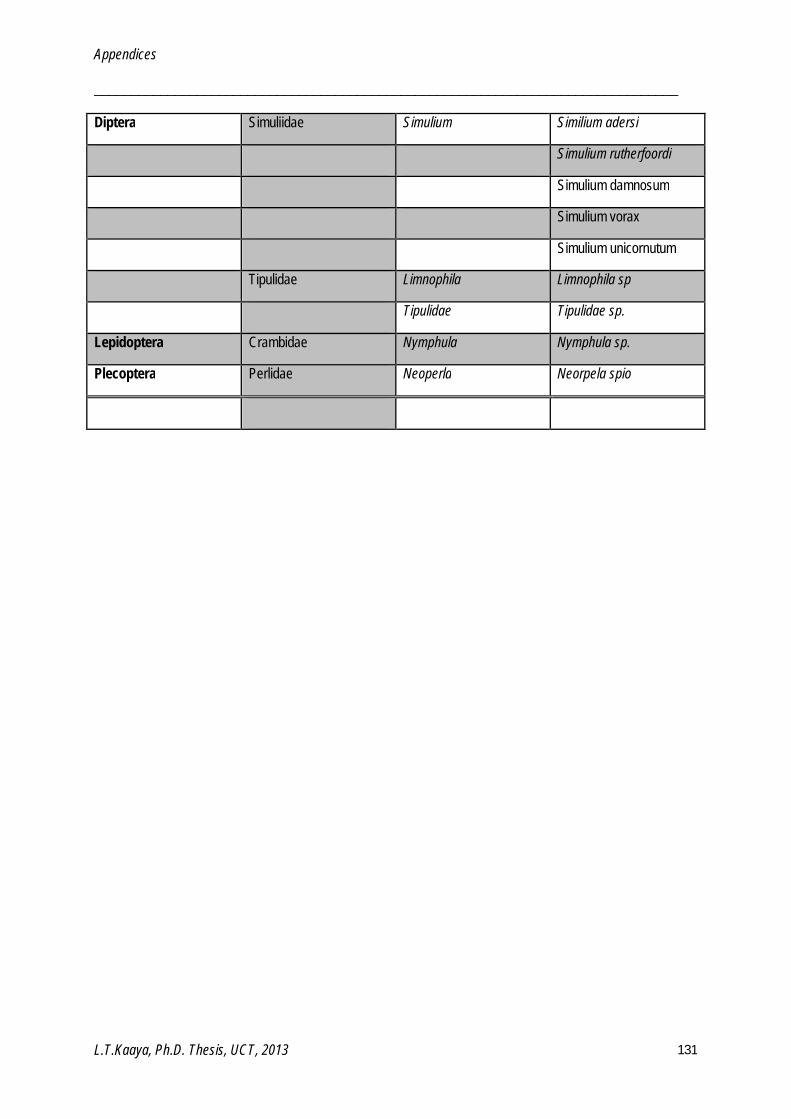
Appendices
________________________________________________________________________________
L.T.Kaaya, Ph.D. Thesis, UCT, 2013 131
Diptera Simuliidae Simulium Similium adersi
Simulium rutherfoordi
Simulium damnosum
Simulium vorax
Simulium unicornutum
Tipulidae Limnophila Limnophila sp
Tipulidae Tipulidae sp.
Lepidoptera Crambidae Nymphula Nymphula sp.
Plecoptera Perlidae Neoperla Neorpela spio

Appendices
________________________________________________________________________________
L.T.Kaaya, Ph.D. Thesis, UCT, 2013 132
Appendix 5.1: TARISS version: 1 scoring sheet showing a list of macroinvertebrate taxa and their respective sensitivity weightings. Columns adjacent to the sensitivity weightings indicate the biotopes at which collected families are to be recorded (S = Stones, V = Vegetation, GSM = Gravel sand mud and C = Combined).

Appendices
________________________________________________________________________________
L.T.Kaaya, Ph.D. Thesis, UCT, 2013 133
Appendix 7.1: Minimum, Median, Maximum and 90th, 67.5th, 45th and 22.5th percentiles of number of taxa, TARISS scores and ASPT of reference sites in PHU, CEAU and CEAL (N = number of sampling occasions).
Number of Taxa TARISS Score ASPT Pangani highland uplands (PHU)
Group 1 (N = 8)
Minimum 18 131 6.2 Median 22 150 7.0 Maximum 32 228 7.4 90th percentile 29 194 7.3 67.5th percentile 25 160 7.1 45th percentile 22 147 7.0 22.5th percentile 19 134 6.5
Group 2 (N = 4)
Minimum 17 105 5.8 Median 24 147 6.2 Maximum 26 162 6.7 90th percentile 25 160 6.6 67.5th percentile 24 154 6.2 45th percentile 23 145 6.2 22.5th percentile 21 129 6.1
Group 2 & 3 (N = 6)
Minimum 12 82 5.8 Median 20 123 6.3 Maximum 26 162 6.8 90th percentile 25 158 6.8 67.5th percentile 23 145 6.5 45th percentile 19 114 6.3 22.5th percentile 14 91 6.2
Central eastern Africa uplands (CEAU)
Group 1( N = 15) Minimum 12 59 4.1 Median 19 108 5.8 Maximum 33 243 8.3 90th percentile 30 208 7.3 67.5th percentile 23 147 6.3 45th percentile 18 103 5.6 22.5th percentile 17 88 5.1
Group 2 (N = 5) Minimum 23 156 6.4 Median 25 170 6.5 Maximum 34 232 7.4 90th percentile 32 212 7.2 67.5th percentile 27 179 6.7 45th percentile 25 168 6.5 22.5th percentile 24 159 6.5
Group 2 & 3 (N = 7) Minimum 23 156 6.4 Median 25 175 6.8 Maximum 34 232 8.1 90th percentile 30 228 7.7
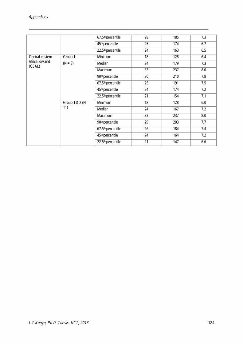
Appendices
________________________________________________________________________________
L.T.Kaaya, Ph.D. Thesis, UCT, 2013 134
67.5th percentile 28 185 7.3 45th percentile 25 174 6.7 22.5th percentile 24 163 6.5
Central eastern Africa lowland (CEAL)
Group 1 (N = 9)
Minimum 18 128 6.4 Median 24 179 7.3 Maximum 33 237 8.0 90th percentile 30 210 7.8 67.5th percentile 25 191 7.5 45th percentile 24 174 7.2 22.5th percentile 21 154 7.1
Group 1 & 2 (N = 11)
Minimum 18 128 6.0 Median 24 167 7.2 Maximum 33 237 8.0 90th percentile 29 203 7.7 67.5th percentile 26 184 7.4 45th percentile 24 164 7.2 22.5th percentile 21 147 6.6