
Logistic Regression and Newton-Raphson · PDF fileLogistic Regression and Newton-Raphson 1.1...
30
Chapter 1 Logistic Regression and Newton-Raphson 1.1 Introduction The logistic regression model is widely used in biomedical settings to model the probability of an event as a function of one or more predictors. For a single predictor X model stipulates that the log odds of “success” is log p 1 - p = β 0 + β 1 X or, equivalently, as p = exp(β 0 + β 1 X ) 1 + exp(β 0 + β 1 X ) where p is the event probability. Depending on the sign of β 1 , p either increases or decreases with X and follows a “sigmoidal” trend. If β 1 =1 then p does not depend on X .
-
Upload
phungkhanh -
Category
Documents
-
view
232 -
download
0
Transcript of Logistic Regression and Newton-Raphson · PDF fileLogistic Regression and Newton-Raphson 1.1...
Chapter 1
Logistic Regression andNewton-Raphson
1.1 Introduction
The logistic regression model is widely used in biomedical settings to model
the probability of an event as a function of one or more predictors. For a
single predictor X model stipulates that the log odds of “success” is
log
(p
1− p
)= β0 + β1X
or, equivalently, as
p =exp(β0 + β1X)
1 + exp(β0 + β1X)
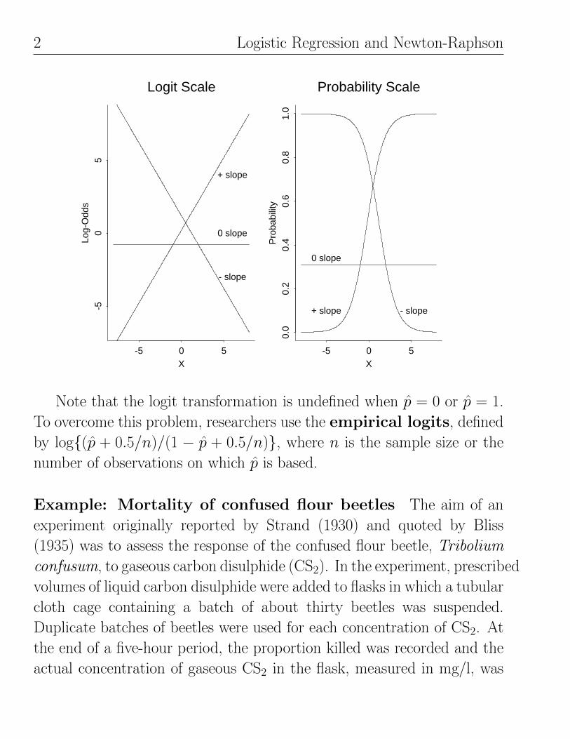
where p is the event probability. Depending on the sign of β1, p either
increases or decreases with X and follows a “sigmoidal” trend. If β1 = 1
then p does not depend on X .
2 Logistic Regression and Newton-Raphson
X
Log-
Odd
s
-5 0 5
-50
5
- slope
+ slope
0 slope
Logit Scale
X
Pro
babi
lity
-5 0 5
0.0
0.2
0.4
0.6
0.8
1.0
0 slope
+ slope - slope
Probability Scale
Note that the logit transformation is undefined when p = 0 or p = 1.
To overcome this problem, researchers use the empirical logits, defined
by log{(p + 0.5/n)/(1 − p + 0.5/n)}, where n is the sample size or the
number of observations on which p is based.
Example: Mortality of confused flour beetles The aim of an
experiment originally reported by Strand (1930) and quoted by Bliss
(1935) was to assess the response of the confused flour beetle, Tribolium
confusum, to gaseous carbon disulphide (CS2). In the experiment, prescribed
volumes of liquid carbon disulphide were added to flasks in which a tubular
cloth cage containing a batch of about thirty beetles was suspended.
Duplicate batches of beetles were used for each concentration of CS2. At
the end of a five-hour period, the proportion killed was recorded and the
actual concentration of gaseous CS2 in the flask, measured in mg/l, was

1.1 Introduction 3
determined by a volumetric analysis. The mortality data are given in the
table below.
## Beetles data set
# conc = CS2 concentration
# y = number of beetles killed
# n = number of beetles exposed
# rep = Replicate number (1 or 2)
beetles <- read.table("http://statacumen.com/teach/SC1/SC1_11_beetles.dat", header = TRUE)
beetles$rep <- factor(beetles$rep)
conc y n rep1 49.06 2 29 12 52.99 7 30 13 56.91 9 28 14 60.84 14 27 15 64.76 23 30 16 68.69 29 31 17 72.61 29 30 18 76.54 29 29 1
conc y n rep9 49.06 4 30 2
10 52.99 6 30 211 56.91 9 34 212 60.84 14 29 213 64.76 29 33 214 68.69 24 28 215 72.61 32 32 216 76.54 31 31 2
Plot the observed probability of mortality and the empirical logits withlinear and quadratic LS fits (which are not the same as the logistic MLEfits).
0.25
0.50
0.75
1.00
50 60 70conc
p.ha
t rep
1
2
Observed mortality, probability scale
−2
0
2
4
50 60 70conc
emp.
logi
t rep
1
2
Empirical logit with `naive' LS fits (not MLE)

4 Logistic Regression and Newton-Raphson
In a number of articles that refer to these data, the responses from
the first two concentrations are omitted because of apparent non-linearity.
Bliss himself remarks that
. . . in comparison with the remaining observations, the two
lowest concentrations gave an exceptionally high kill. Over the
remaining concentrations, the plotted values seemed to form
a moderately straight line, so that the data were handled as
two separate sets, only the results at 56.91 mg of CS2 per litre
being included in both sets.
However, there does not appear to be any biological motivation for this
and so here they are retained in the data set.
Combining the data from the two replicates and plotting the empirical
logit of the observed proportions against concentration gives a relationship
that is better fit by a quadratic than a linear relationship,
log
(p
1− p
)= β0 + β1X + β2X
2.
The right plot below shows the linear and quadratic model fits to the
observed values with point-wise 95% confidence bands on the logit scale,
and on the left is the same on the proportion scale.

1.2 The Model 5
●
●
●
●
●
●
●
●
●
●
●
●
●
●
●●
0.00
0.25
0.50
0.75
1.00
50 60 70conc
p.ha
t
modelorder
●
●
linear
quadratic
rep
● 1
2
Observed and predicted mortality, probability scale
●
●
●
●
●
●
●
●
●
●
●
●
●
●
●
●
−2.5
0.0
2.5
5.0
7.5
50 60 70conc
emp.
logi
t
modelorder
●
●
linear
quadratic
rep
● 1
2
Observed and predicted mortality, logit scale
We will focus on how to estimate parameters of a logistic regression
model using maximum likelihood (MLEs).
1.2 The Model
Suppose Yiind∼ Binomial(mi, pi) random variables, i = 1, 2, . . . , n. For
example, Yi is the number of beetle deaths from a total of mi beetles at
concentration Xi over the i = 1, 2, . . . , n concentrations. Note that mi
can equal 1 (and often does in observational studies). Recall that the
probability mass function for a Binomial is
Pr[Yi = yi|pi] =
(mi
yi
)pyii (1− pi)mi−yi, yi = 0, 1, 2, . . . ,mi.
So the joint distribution of Y1, Y2, . . . , Yn is
Pr[Y1 = y1, . . . , Yn = yn|p1, . . . , pn] =
n∏i=1
(mi
yi
)pyii (1− pi)mi−yi.
6 Logistic Regression and Newton-Raphson
The log-likelihood, ignoring the constant, is
` = log {Pr[Y1 = y1, . . . , Yn = yn|p1, . . . , pn]}
∝ log
{n∏i=1
pyii (1− pi)mi−yi
}
=
n∑i=1
{yi log(pi) + (mi − yi) log(1− pi)}
=
n∑i=1
{mi log(1− pi) + yi log
(pi
1− pi
)}. (1.1)
The logistic regression model assumes that pi depends on r covariates
xi1, xi2, . . . , xir through
log
(pi
1− pi
)= β0 + β1xi1 + · · · + βrxir
=[
1 xi1 xi2 · · · xir]β0
β1
β2...
βr
= x˜>i β˜.
The covariates or predictors are fixed, while β˜ is an unknown parameter
vector. Regardless, pi is a function of both x˜i and β˜,
pi ≡ pi(x˜i, β˜) or pi(β˜) (suppressing x˜i, since it is known).

1.2 The Model 7
Note that the model implies
pi =exp(x˜>i β˜)
1 + exp(x˜>i β˜)and
1− pi =1
1 + exp(x˜>i β˜).
To obtain the MLEs we first write the log-likelihood in (1.1) as a function
of β˜,
`(β˜) =
n∑i=1
mi log
(1
1 + exp(x˜>i β˜)
)+ yi log
exp(x˜>i β˜)
1+exp(x˜>i β˜)
11+exp(x˜>i β˜)
=
n∑i=1
{mi log
(1
1 + exp(x˜>i β˜)
)+ yi(x˜>i β˜)
}
=
n∑i=1
{yi(x˜>i β˜)−mi log(1 + exp(x˜>i β˜))
}. (1.2)
To maximize `(β˜), we compute the score function
˙(β˜) =
∂`(β˜)/∂β0
∂`(β˜)/∂β1...
∂`(β˜)/∂βr
and solve the likelihood equations
˙(β˜) = 0˜r+1.
8 Logistic Regression and Newton-Raphson
Note that ˙(β˜) is an (r + 1)-by-1 vector, so we are solving a system of
r + 1 non-linear equations.
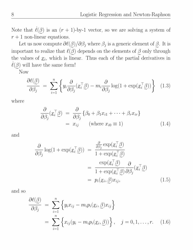
Let us now compute ∂`(β˜)/∂βj where βj is a generic element of β˜. It is
important to realize that `(β˜) depends on the elements of β˜ only through
the values of x˜i, which is linear. Thus each of the partial derivatives in˙(β˜) will have the same form!
Now
∂`(β˜)
∂βj=
n∑i=1
{yi∂
∂βj(x˜>i β˜)−mi
∂
∂βjlog(1 + exp(x˜>i β˜))
}(1.3)
where
∂
∂βj(x˜>i β˜) =
∂
∂βj{β0 + β1xi1 + · · · + βrxir}
= xij (where xi0 ≡ 1) (1.4)
and
∂
∂βjlog(1 + exp(x˜>i β˜)) =
∂∂βj
exp(x˜>i β˜)
1 + exp(x˜>i β˜)
=exp(x˜>i β˜)
1 + exp(x˜>i β˜)
∂
∂βj(x˜>i β˜)
= pi(x˜i, β˜)xij, (1.5)
and so
∂`(β˜)
∂βj=
n∑i=1
{yixij −mipi(x˜i, β˜)xij
}=
n∑i=1
{xij(yi −mipi(x˜i, β˜))
}, j = 0, 1, . . . , r. (1.6)
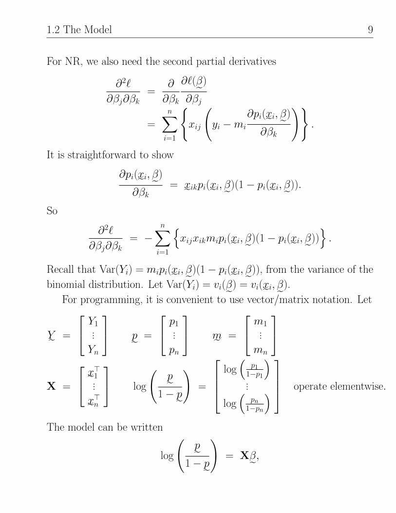
1.2 The Model 9
For NR, we also need the second partial derivatives
∂2`
∂βj∂βk=
∂
∂βk
∂`(β˜)
∂βj
=
n∑i=1
{xij
(yi −mi
∂pi(x˜i, β˜)
∂βk
)}.
It is straightforward to show
∂pi(x˜i, β˜)
∂βk= x˜ikpi(x˜i, β˜)(1− pi(x˜i, β˜)).
So
∂2`
∂βj∂βk= −
n∑i=1
{xijxikmipi(x˜i, β˜)(1− pi(x˜i, β˜))
}.
Recall that Var(Yi) = mipi(x˜i, β˜)(1− pi(x˜i, β˜)), from the variance of the
binomial distribution. Let Var(Yi) = vi(β˜) = vi(x˜i, β˜).
For programming, it is convenient to use vector/matrix notation. Let
Y˜ =
Y1...
Yn
p˜ =
p1...
pn
m˜ =
m1...
mn
X =
x˜>1...x˜>n log
(p˜
1− p˜)
=
log(
p11−p1
)...
log(
pn1−pn
) operate elementwise.
The model can be written
log
(p˜
1− p˜)
= Xβ˜,
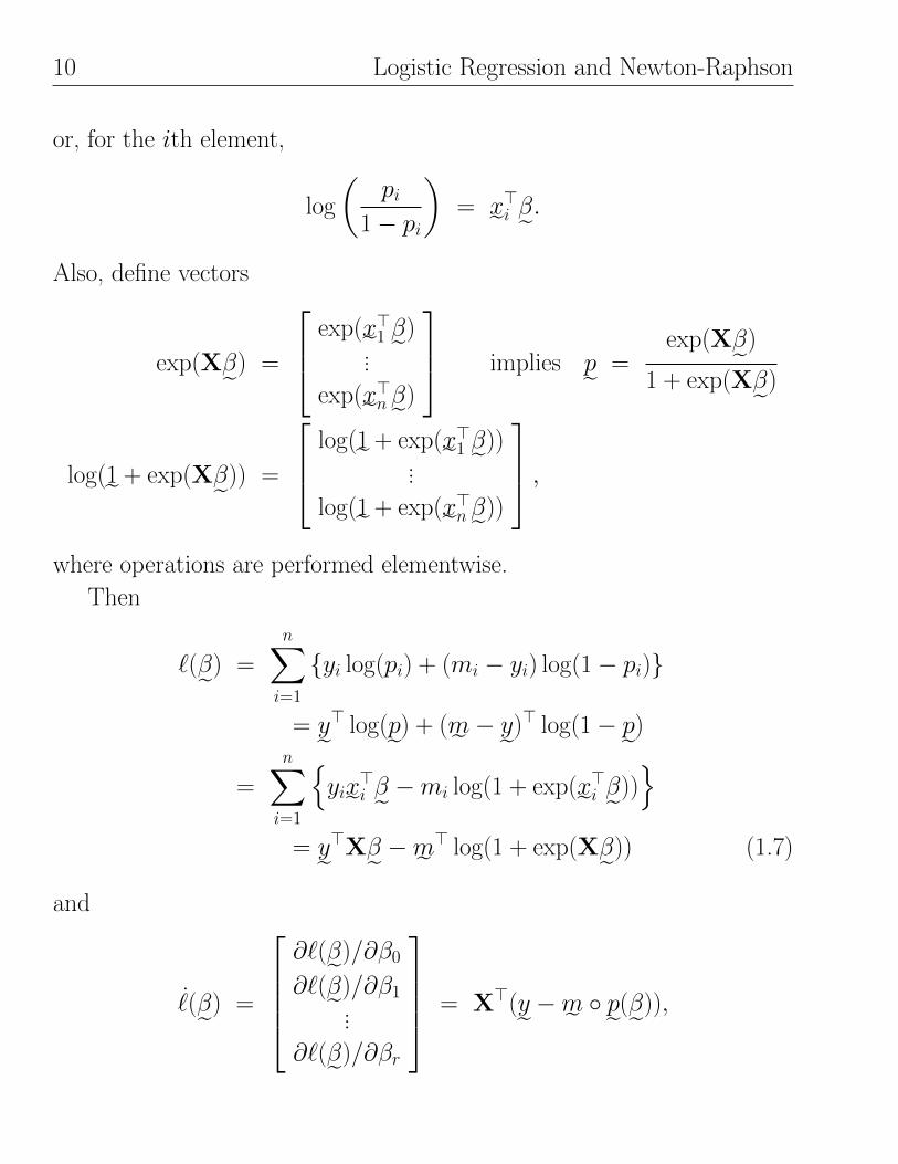
10 Logistic Regression and Newton-Raphson
or, for the ith element,
log
(pi
1− pi
)= x˜>i β˜.
Also, define vectors
exp(Xβ˜) =
exp(x˜>1 β˜)...
exp(x˜>nβ˜)
implies p˜ =exp(Xβ˜)
1 + exp(Xβ˜)
log(1˜+ exp(Xβ˜)) =
log(1˜+ exp(x˜>1 β˜))...
log(1˜+ exp(x˜>nβ˜))
,where operations are performed elementwise.
Then
`(β˜) =
n∑i=1
{yi log(pi) + (mi − yi) log(1− pi)}
= y˜> log(p˜) + (m˜ − y˜)> log(1− p˜)
=
n∑i=1
{yix˜>i β˜ −mi log(1 + exp(x˜>i β˜))
}= y˜>Xβ˜ −m˜> log(1 + exp(Xβ˜)) (1.7)
and
˙(β˜) =
∂`(β˜)/∂β0
∂`(β˜)/∂β1...
∂`(β˜)/∂βr
= X>(y˜−m˜ ◦ p˜(β˜)),
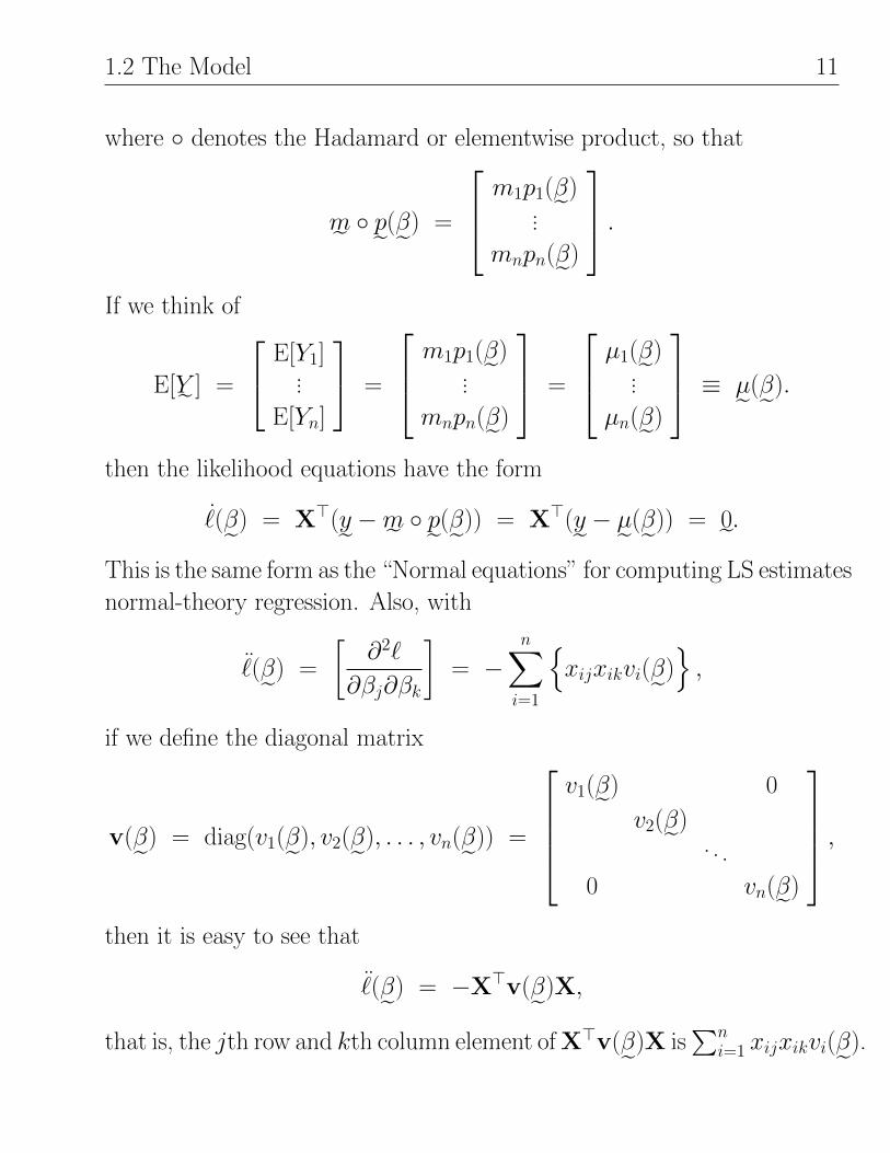
1.2 The Model 11
where ◦ denotes the Hadamard or elementwise product, so that
m˜ ◦ p˜(β˜) =
m1p1(β˜)...
mnpn(β˜)
.If we think of
E[Y˜ ] =
E[Y1]...
E[Yn]
=
m1p1(β˜)...
mnpn(β˜)
=
µ1(β˜)...
µn(β˜)
≡ µ˜(β˜).
then the likelihood equations have the form
˙(β˜) = X>(y˜−m˜ ◦ p˜(β˜)) = X>(y˜− µ˜(β˜)) = 0˜.This is the same form as the “Normal equations” for computing LS estimates
normal-theory regression. Also, with
¨(β˜) =
[∂2`
∂βj∂βk
]= −
n∑i=1
{xijxikvi(β˜)
},
if we define the diagonal matrix
v(β˜) = diag(v1(β˜), v2(β˜), . . . , vn(β˜)) =
v1(β˜) 0
v2(β˜). . .
0 vn(β˜)
,then it is easy to see that
¨(β˜) = −X>v(β˜)X,
that is, the jth row and kth column element of X>v(β˜)X is∑n
i=1 xijxikvi(β˜).
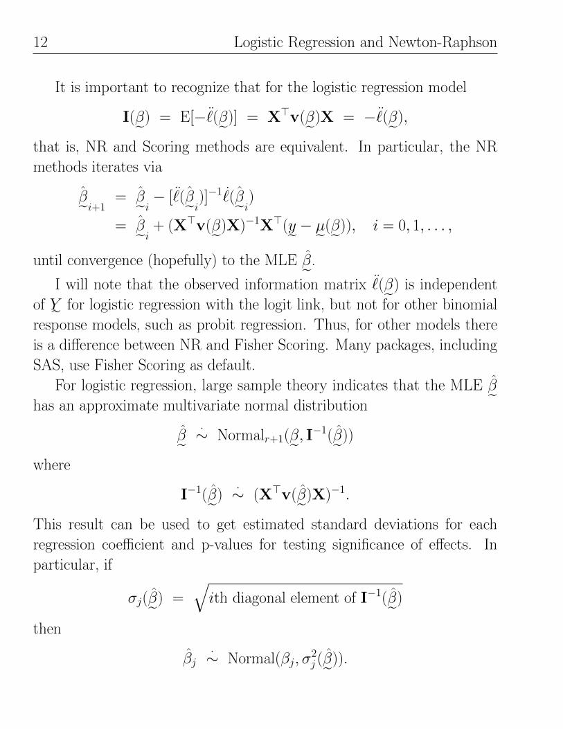
12 Logistic Regression and Newton-Raphson
It is important to recognize that for the logistic regression model
I(β˜) = E[− ¨(β˜)] = X>v(β˜)X = − ¨(β˜),
that is, NR and Scoring methods are equivalent. In particular, the NR
methods iterates via
β˜i+1= β˜i − [ ¨(β˜i)]−1 ˙(β˜i)= β˜i + (X>v(β˜)X)−1X>(y˜− µ˜(β˜)), i = 0, 1, . . . ,
until convergence (hopefully) to the MLE β˜.
I will note that the observed information matrix ¨(β˜) is independent
of Y˜ for logistic regression with the logit link, but not for other binomial
response models, such as probit regression. Thus, for other models there
is a difference between NR and Fisher Scoring. Many packages, including
SAS, use Fisher Scoring as default.
For logistic regression, large sample theory indicates that the MLE β˜has an approximate multivariate normal distribution
β˜ ·∼ Normalr+1(β˜, I−1(β˜))
where
I−1(β˜)·∼ (X>v(β˜)X)−1.
This result can be used to get estimated standard deviations for each
regression coefficient and p-values for testing significance of effects. In
particular, if
σj(β˜) =√ith diagonal element of I−1(β˜)
then
βj·∼ Normal(βj, σ
2j (β˜)).
1.2 The Model 13
A p-value for testing H0 : βj = 0 can be based on
βj − 0
σj(β˜)
·∼ Normal(0, 1).
General remarks
1. There is an extensive literature on conditions for existence and uniqueness
of MLEs for logistic regression.
2. MLEs may not exist. One case is when you have “separation” of
covariates (e.g., all successes to left and all failures to right for some
value of x).
3. Convergence is sensitive to starting values.
For the model
log
(pi
1− pi
)= β0 + β1xi1 + · · · + βrxir
the following starting values often work well, especially if regression
effects are not too strong:
β0 start = log
(p
1− p
)= log
( ∑ni=1
yimi
1−∑n
i=1yimi
)= log
( ∑ni=1 yi∑n
i=1(mi − yi)
),
and β1 start = · · · = βr start = 0, where p =∑n
i=1yimi
is the overall
proportion. This is the MLE for β0 if β1 = · · · = βr = 0.
14 Logistic Regression and Newton-Raphson
4. If you have two observations Y1ind∼ Binomial(m1, p) and Y2
ind∼Binomial(m2, p) with the same success probability p, then the log-
likelihood (excluding constants) is the same regardless of whether
you treat Y1 and Y2 as separate binomial observations or you combine
them as Y1 +Y2ind∼ Binomial(m1 +m2, p). More generally, Bernoulli
observations with the same covariate vector can be combined into
a single binomial response (provided observations are independent)
when defining the log-likelihood.
1.3 Implementation
Function f.lr.p() computes the probability vector under a logistic regression
model
pi =exp(x˜>i β˜)
1 + exp(x˜>i β˜)
from the design matrix X and regression vector β˜. The function assumes
that X and β˜ are of the correct dimensions.
f.lr.p <- function(X, beta) {# compute vector p of probabilities for logistic regression with logit link
X <- as.matrix(X)
beta <- as.vector(beta)
p <- exp(X %*% beta) / (1 + exp(X %*% beta))
return(p)
}
Function f.lr.l() computes the binomial log-likelihood function
` ∝n∑i=1
{yi log(pi) + (mi − yi) log(1− pi)} (1.8)
1.3 Implementation 15
from three input vectors: the counts y˜, the sample sizes m˜ , and the
probabilities p˜. The function is arbitrary, working for all Binomial models.
f.lr.l <- function(y, m, p) {# binomial log likelihood function
# input: vectors: y = counts; m = sample sizes; p = probabilities
# output: log-likelihood l, a scalar
l <- t(y) %*% log(p) + t(m - y) %*% log(1 - p)
return(l)
}
The Fisher’s scoring routine for logistic regression f.lr.FS() finds the
MLE β˜ (without line-search), following from the derivation above.
Convergence is based on the number of iterations, maxit = 50, Euclidean
distance between successive iterations of β˜, eps1, and distance between
successive iterations of the log-likelihood, eps2. The absolute difference
in log-likelihoods between successive steps is new for us, but a sensible
addition.
Comments
1. The iteration scheme
β˜i+1= β˜i + (X>v(β˜)X)−1X>(y˜− µ˜(β˜))
= β˜i + (inverse Info)(Score func)
is implemented below in two ways. The commented method takes
the inverse of the information matrix, which can be computationally
intensive and (occasionally) numerically unstable. The uncommented
method solves
(X>v(β˜)X)(β˜i+1− β˜i) = X>(y˜− µ˜(β˜))
for (increm) = (β˜i+1−β˜i). The new estimate is β˜i+1
= β˜i+(increm).

16 Logistic Regression and Newton-Raphson
2. Line search is implemented by evaluating the log-likelihood over a
range (−1, 2) of α step sizes and choosing the step that gives the
largest log-likelihood.
3. It calls both f.lr.l(), the function to calculate log-likelihood, and
f.lr.p(), the function to compute vector p of probabilities for LR.
f.lr.FS <- function(X, y, m, beta.1
, eps1 = 1e-6, eps2 = 1e-7, maxit = 50) {# Fisher's scoring routine for estimation of LR model (with line search)
# Input:
# X = n-by-(r+1) design matrix
# y = n-by-1 vector of success counts
# m = n-by-1 vector of sample sizes
# beta.1 = (r+1)-by-1 vector of starting values for regression est
# Iteration controlled by:
# eps1 = absolute convergence criterion for beta
# eps2 = absolute convergence criterion for log-likelihood
# maxit = maximum allowable number of iterations
# Output:
# out = list containing:
# beta.MLE = beta MLE
# NR.hist = iteration history of convergence differences
# beta.hist = iteration history of beta
# beta.cov = beta covariance matrix (inverse Fisher's information matrix at MLE)
# note = convergence note
beta.2 <- rep(-Inf, length(beta.1)) # init beta.2
diff.beta <- sqrt(sum((beta.1 - beta.2)^2)) # Euclidean distance
llike.1 <- f.lr.l(y, m, f.lr.p(X, beta.1)) # update loglikelihood
llike.2 <- f.lr.l(y, m, f.lr.p(X, beta.2)) # update loglikelihood
diff.like <- abs(llike.1 - llike.2) # diff
if (is.nan(diff.like)) { diff.like <- 1e9 }
i <- 1 # initial iteration index
alpha.step <- seq(-1, 2, by = 0.1)[-11] # line search step sizes, excluding 0
NR.hist <- data.frame(i, diff.beta, diff.like, llike.1, step.size = 1) # iteration history
beta.hist <- matrix(beta.1, nrow = 1)
while ((i <= maxit) & (diff.beta > eps1) & (diff.like > eps2)) {

1.3 Implementation 17
i <- i + 1 # increment iteration
# update beta
beta.2 <- beta.1 # old guess is current guess
mu.2 <- m * f.lr.p(X, beta.2) # m * p is mean
# variance matrix
v.2 <- diag(as.vector(m * f.lr.p(X, beta.2) * (1 - f.lr.p(X, beta.2))))
score.2 <- t(X) %*% (y - mu.2) # score function
# this increment version inverts the information matrix
# Iinv.2 <- solve(t(X) %*% v.2 %*% X) # Inverse information matrix
# increm <- Iinv.2 %*% score.2 # increment, solve() is inverse
# this increment version solves for (beta.2-beta.1) without inverting Information
increm <- solve(t(X) %*% v.2 %*% X, score.2) # solve for increment
# line search for improved step size
llike.alpha.step <- rep(NA, length(alpha.step)) # init llike for line search
for (i.alpha.step in 1:length(alpha.step)) {llike.alpha.step[i.alpha.step] <- f.lr.l(y, m
, f.lr.p(X, beta.2 + alpha.step[i.alpha.step] * increm))
}# step size index for max increase in log-likelihood (if tie, [1] takes first)
ind.max.alpha.step <- which(llike.alpha.step == max(llike.alpha.step))[1]
beta.1 <- beta.2 + alpha.step[ind.max.alpha.step] * increm # update beta
diff.beta <- sqrt(sum((beta.1 - beta.2)^2)) # Euclidean distance
llike.2 <- llike.1 # age likelihood value
llike.1 <- f.lr.l(y, m, f.lr.p(X, beta.1)) # update loglikelihood
diff.like <- abs(llike.1 - llike.2) # diff
# iteration history
NR.hist <- rbind(NR.hist, c(i, diff.beta, diff.like, llike.1, alpha.step[ind.max.alpha.step]))
beta.hist <- rbind(beta.hist, matrix(beta.1, nrow = 1))
}
# prepare output
out <- list()
out$beta.MLE <- beta.1
out$iter <- i - 1
out$NR.hist <- NR.hist
out$beta.hist <- beta.hist
v.1 <- diag(as.vector(m * f.lr.p(X, beta.1) * (1 - f.lr.p(X, beta.1))))
Iinv.1 <- solve(t(X) %*% v.1 %*% X) # Inverse information matrix
out$beta.cov <- Iinv.1

18 Logistic Regression and Newton-Raphson
if (!(diff.beta > eps1) & !(diff.like > eps2)) {out$note <- paste("Absolute convergence of", eps1, "for betas and"
, eps2, "for log-likelihood satisfied")
}if (i > maxit) {
out$note <- paste("Exceeded max iterations of ", maxit)
}return(out)
}
1.3.1 Example (cont.): Mortality of confused flourbeetles
Load the beetles dataset and fit quadratic model. The model is
log
(p
1− p
)= β0 + β1X + β2X
2.
where X = CS2 level.
## Beetles data set
# conc = CS2 concentration
# y = number of beetles killed
# n = number of beetles exposed
# rep = Replicate number (1 or 2)
beet <- read.table("http://statacumen.com/teach/SC1/SC1_11_beetles.dat", header = TRUE)
beet$rep <- factor(beet$rep)
# create data variables: m, y, X
n <- nrow(beet)
m <- beet$n
y <- beet$y
X.temp <- beet$conc
# quadratic model
X <- matrix(c(rep(1,n), X.temp, X.temp^2), nrow = n)
colnames(X) <- c("Int", "conc", "conc2")
r <- ncol(X) - 1 # number of regression coefficients - 1
1.3 Implementation 19
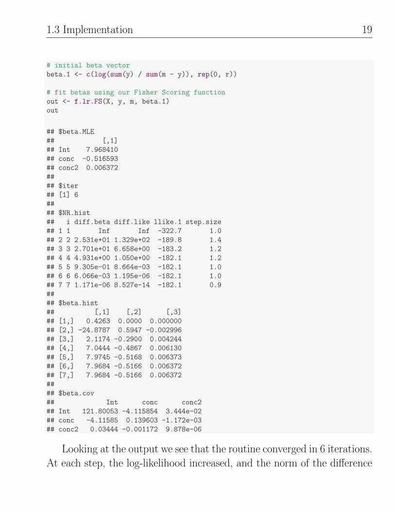
# initial beta vector
beta.1 <- c(log(sum(y) / sum(m - y)), rep(0, r))
# fit betas using our Fisher Scoring function
out <- f.lr.FS(X, y, m, beta.1)
out
## $beta.MLE
## [,1]
## Int 7.968410
## conc -0.516593
## conc2 0.006372
##
## $iter
## [1] 6
##
## $NR.hist
## i diff.beta diff.like llike.1 step.size
## 1 1 Inf Inf -322.7 1.0
## 2 2 2.531e+01 1.329e+02 -189.8 1.4
## 3 3 2.701e+01 6.658e+00 -183.2 1.2
## 4 4 4.931e+00 1.050e+00 -182.1 1.2
## 5 5 9.305e-01 8.664e-03 -182.1 1.0
## 6 6 6.066e-03 1.195e-06 -182.1 1.0
## 7 7 1.171e-06 8.527e-14 -182.1 0.9
##
## $beta.hist
## [,1] [,2] [,3]
## [1,] 0.4263 0.0000 0.000000
## [2,] -24.8787 0.5947 -0.002996
## [3,] 2.1174 -0.2900 0.004244
## [4,] 7.0444 -0.4867 0.006130
## [5,] 7.9745 -0.5168 0.006373
## [6,] 7.9684 -0.5166 0.006372
## [7,] 7.9684 -0.5166 0.006372
##
## $beta.cov
## Int conc conc2
## Int 121.80053 -4.115854 3.444e-02
## conc -4.11585 0.139603 -1.172e-03
## conc2 0.03444 -0.001172 9.878e-06
Looking at the output we see that the routine converged in 6 iterations.
At each step, the log-likelihood increased, and the norm of the difference
20 Logistic Regression and Newton-Raphson
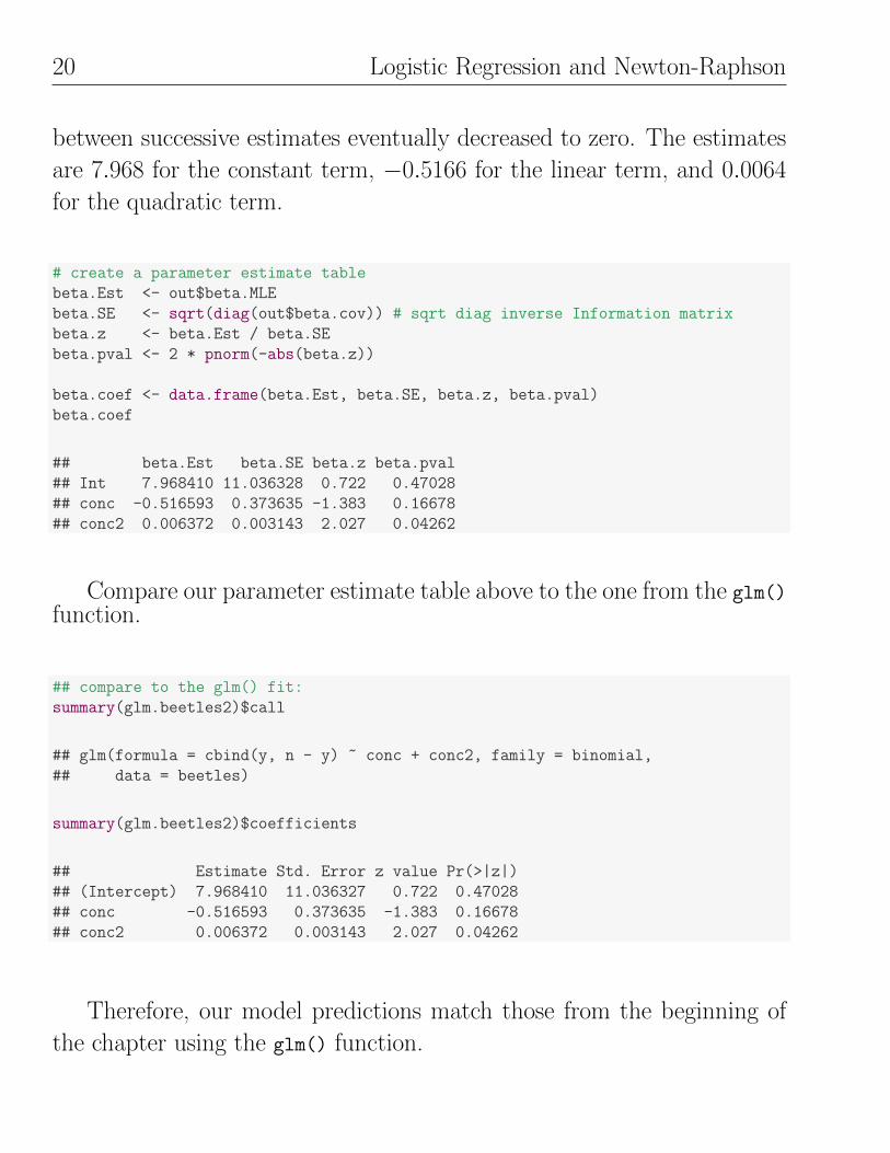
between successive estimates eventually decreased to zero. The estimates
are 7.968 for the constant term, −0.5166 for the linear term, and 0.0064
for the quadratic term.
# create a parameter estimate table
beta.Est <- out$beta.MLE
beta.SE <- sqrt(diag(out$beta.cov)) # sqrt diag inverse Information matrix
beta.z <- beta.Est / beta.SE
beta.pval <- 2 * pnorm(-abs(beta.z))
beta.coef <- data.frame(beta.Est, beta.SE, beta.z, beta.pval)
beta.coef
## beta.Est beta.SE beta.z beta.pval
## Int 7.968410 11.036328 0.722 0.47028
## conc -0.516593 0.373635 -1.383 0.16678
## conc2 0.006372 0.003143 2.027 0.04262
Compare our parameter estimate table above to the one from the glm()function.
## compare to the glm() fit:
summary(glm.beetles2)$call
## glm(formula = cbind(y, n - y) ~ conc + conc2, family = binomial,
## data = beetles)
summary(glm.beetles2)$coefficients
## Estimate Std. Error z value Pr(>|z|)
## (Intercept) 7.968410 11.036327 0.722 0.47028
## conc -0.516593 0.373635 -1.383 0.16678
## conc2 0.006372 0.003143 2.027 0.04262
Therefore, our model predictions match those from the beginning of
the chapter using the glm() function.

1.3 Implementation 21
●
●
●
●
●
●
●●
0.25
0.50
0.75
1.00
50 60 70conc
p.ha
t rep
● 1
2
FS Observed and predicted mortality, probability scale
●
●
●
●
●
●
●●
0.25
0.50
0.75
1.00
50 60 70conc
p.ha
t rep
● 1
2
glm Observed and predicted mortality, probability scale
Also note that the observed and fitted proportions are fairly close,
which qualitatively suggests a reasonable model for the data.
1.3.2 Example: Leukemia white blood cell types
This example illustrates modeling with continuous and factor predictors.
Feigl and Zelen1 reported the survival time in weeks and the white cell
blood count (WBC) at time of diagnosis for 33 patients who eventually
died of acute leukemia. Each person was classified as AG+ or AG−,
indicating the presence or absence of a certain morphological characteristic
in the white cells. Four variables are given in the data set: WBC, a binary
factor or indicator variable AG (1 for AG+, 0 for AG−), NTOTAL
(the number of patients with the given combination of AG and WBC),
1Feigl, P., Zelen, M. (1965) Estimation of exponential survival probabilities with concomitantinformation. Biometrics 21, 826–838. Survival times are given for 33 patients who died from acutemyelogenous leukaemia. Also measured was the patient’s white blood cell count at the time ofdiagnosis. The patients were also factored into 2 groups according to the presence or absence of amorphologic characteristic of white blood cells. Patients termed AG positive were identified by thepresence of Auer rods and/or significant granulation of the leukaemic cells in the bone marrow atthe time of diagnosis.

22 Logistic Regression and Newton-Raphson
and NRES (the number of NTOTAL that survived at least one year from
the time of diagnosis).
The researchers are interested in modelling the probability p of surviving
at least one year as a function of WBC and AG. They believe that WBC
should be transformed to a log scale, given the skewness in the WBC
values.
## Leukemia white blood cell types example
# ntotal = number of patients with IAG and WBC combination
# nres = number surviving at least one year
# ag = 1 for AG+, 0 for AG-
# wbc = white cell blood count
# lwbc = log white cell blood count
# p.hat = Emperical Probability
leuk <- read.table("http://statacumen.com/teach/SC1/SC1_11_leuk.dat", header = TRUE)
leuk$lwbc <- log(leuk$wbc)
leuk$p.hat <- leuk$nres / leuk$ntotal
ntotal nres ag wbc lwbc p.hat1 1 1 1 75 4.32 1.002 1 1 1 230 5.44 1.003 1 1 1 260 5.56 1.004 1 1 1 430 6.06 1.005 1 1 1 700 6.55 1.006 1 1 1 940 6.85 1.007 1 1 1 1000 6.91 1.008 1 1 1 1050 6.96 1.009 3 1 1 10000 9.21 0.3310 1 1 0 300 5.70 1.0011 1 1 0 440 6.09 1.0012 1 0 1 540 6.29 0.0013 1 0 1 600 6.40 0.0014 1 0 1 1700 7.44 0.0015 1 0 1 3200 8.07 0.0016 1 0 1 3500 8.16 0.0017 1 0 1 5200 8.56 0.0018 1 0 0 150 5.01 0.0019 1 0 0 400 5.99 0.0020 1 0 0 530 6.27 0.0021 1 0 0 900 6.80 0.0022 1 0 0 1000 6.91 0.0023 1 0 0 1900 7.55 0.0024 1 0 0 2100 7.65 0.0025 1 0 0 2600 7.86 0.0026 1 0 0 2700 7.90 0.0027 1 0 0 2800 7.94 0.0028 1 0 0 3100 8.04 0.0029 1 0 0 7900 8.97 0.0030 2 0 0 10000 9.21 0.00
1.3 Implementation 23
As an initial step in the analysis, consider the following model:
log
(p
1− p
)= β0 + β1LWBC + β2AG,
where LWBC = log(WBC). The model is best understood by separating
the AG+ and AG− cases. For AG− individuals, AG=0 so the model
reduces to
log
(p
1− p
)= β0 + β1LWBC + β2 ∗ 0 = β0 + β1LWBC.
For AG+ individuals, AG=1 and the model implies
log
(p
1− p
)= β0 + β1LWBC + β2 ∗ 1 = (β0 + β2) + β1LWBC.
The model without AG (i.e., β2 = 0) is a simple logistic model where
the log-odds of surviving one year is linearly related to LWBC, and is
independent of AG. The reduced model with β2 = 0 implies that there is
no effect of the AG level on the survival probability once LWBC has been
taken into account.
Including the binary predictor AG in the model implies that there
is a linear relationship between the log-odds of surviving one year and
LWBC, with a constant slope for the two AG levels. This model includes
an effect for the AG morphological factor, but more general models are
possible. A natural extension would be to include a product or interaction
effect, a point that I will return to momentarily.
The parameters are easily interpreted: β0 and β0 +β2 are intercepts for
the population logistic regression lines for AG− and AG+, respectively.
The lines have a common slope, β1. The β2 coefficient for the AG indicator
is the difference between intercepts for the AG+ and AG− regression lines.
24 Logistic Regression and Newton-Raphson
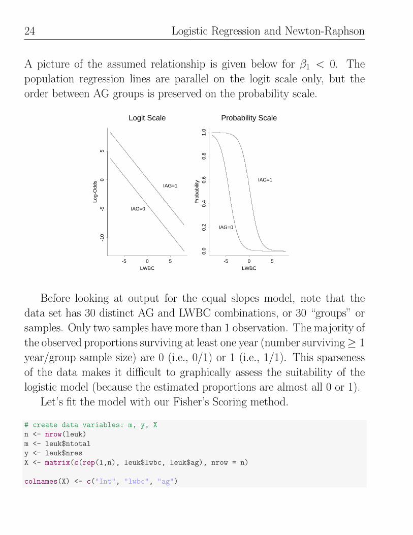
A picture of the assumed relationship is given below for β1 < 0. The
population regression lines are parallel on the logit scale only, but the
order between AG groups is preserved on the probability scale.
LWBC
Log-
Odd
s
-5 0 5
-10
-50
5
IAG=1
IAG=0
Logit Scale
LWBC
Pro
babi
lity
-5 0 5
0.0
0.2
0.4
0.6
0.8
1.0
IAG=0
IAG=1
Probability Scale
Before looking at output for the equal slopes model, note that the
data set has 30 distinct AG and LWBC combinations, or 30 “groups” or
samples. Only two samples have more than 1 observation. The majority of
the observed proportions surviving at least one year (number surviving≥ 1
year/group sample size) are 0 (i.e., 0/1) or 1 (i.e., 1/1). This sparseness
of the data makes it difficult to graphically assess the suitability of the
logistic model (because the estimated proportions are almost all 0 or 1).
Let’s fit the model with our Fisher’s Scoring method.
# create data variables: m, y, X
n <- nrow(leuk)
m <- leuk$ntotal
y <- leuk$nres
X <- matrix(c(rep(1,n), leuk$lwbc, leuk$ag), nrow = n)
colnames(X) <- c("Int", "lwbc", "ag")

1.3 Implementation 25
r <- ncol(X) - 1 # number of regression coefficients - 1
# initial beta vector
beta.1 <- c(log(sum(y) / sum(m - y)), rep(0, r))
# fit betas using our Fisher Scoring function
out <- f.lr.FS(X, y, m, beta.1)
out
## $beta.MLE
## [,1]
## Int 5.543
## lwbc -1.109
## ag 2.520
##
## $iter
## [1] 5
##
## $NR.hist
## i diff.beta diff.like llike.1 step.size
## 1 1 Inf 1.000e+09 -21.00 1.0
## 2 2 6.081e+00 7.168e+00 -13.84 1.3
## 3 3 5.602e-01 4.164e-01 -13.42 1.2
## 4 4 1.814e-01 4.077e-03 -13.42 1.0
## 5 5 3.747e-03 1.267e-06 -13.42 1.0
## 6 6 1.368e-06 1.901e-13 -13.42 0.9
##
## $beta.hist
## [,1] [,2] [,3]
## [1,] -0.6931 0.0000 0.000
## [2,] 4.9039 -0.9312 2.188
## [3,] 5.3702 -1.0819 2.460
## [4,] 5.5399 -1.1082 2.518
## [5,] 5.5433 -1.1088 2.520
## [6,] 5.5433 -1.1088 2.520
##
## $beta.cov
## Int lwbc ag
## Int 9.1350 -1.3400 0.4507
## lwbc -1.3400 0.2125 -0.1798
## ag 0.4507 -0.1798 1.1896
Looking at the output we see that the routine converged in 5 iterations.

26 Logistic Regression and Newton-Raphson
At each step, the log-likelihood increased, and the norm of the difference
between successive estimates eventually decreased to zero. The estimates
are 5.543 for the constant term, −1.109 for the linear term, and 2.52 for
the quadratic term.
# create a parameter estimate table
beta.Est <- out$beta.MLE
beta.SE <- sqrt(diag(out$beta.cov)) # sqrt diag inverse Information matrix
beta.z <- beta.Est / beta.SE
beta.pval <- 2 * pnorm(-abs(beta.z))
beta.coef <- data.frame(beta.Est, beta.SE, beta.z, beta.pval)
beta.coef
## beta.Est beta.SE beta.z beta.pval
## Int 5.543 3.0224 1.834 0.06664
## lwbc -1.109 0.4609 -2.405 0.01616
## ag 2.520 1.0907 2.310 0.02088
Compare our parameter estimate table above to the one from the glm()
function.
## compare to the glm() fit:
summary(glm.i.l)$call
## glm(formula = cbind(nres, ntotal - nres) ~ ag + lwbc, family = binomial,
## data = leuk)
summary(glm.i.l)$coefficients
## Estimate Std. Error z value Pr(>|z|)
## (Intercept) 5.543 3.0224 1.834 0.06664
## ag1 2.520 1.0907 2.310 0.02088
## lwbc -1.109 0.4609 -2.405 0.01615
Given that the model fits reasonably well, a test of H0 : β2 = 0 might
be a primary interest here. This checks whether the regression lines are
identical for the two AG levels, which is a test for whether AG affects the
1.3 Implementation 27
survival probability, after taking LWBC into account. This test is rejected
at any of the usual significance levels, suggesting that the AG level affects
the survival probability (assuming a very specific model).
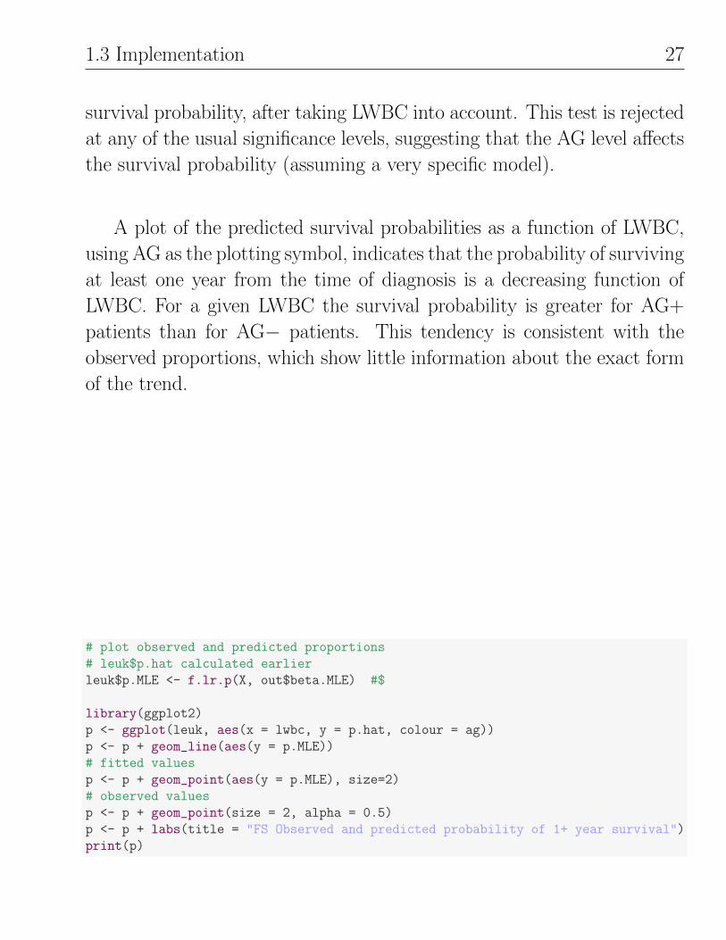
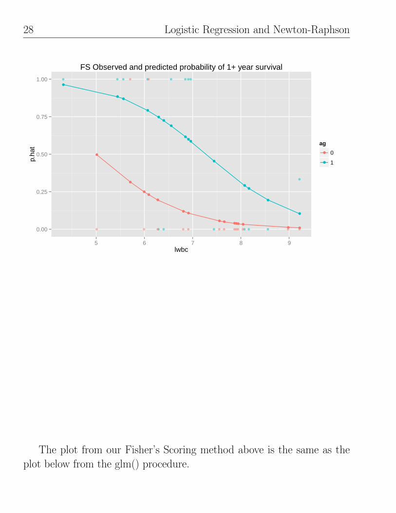
A plot of the predicted survival probabilities as a function of LWBC,
using AG as the plotting symbol, indicates that the probability of surviving
at least one year from the time of diagnosis is a decreasing function of
LWBC. For a given LWBC the survival probability is greater for AG+
patients than for AG− patients. This tendency is consistent with the
observed proportions, which show little information about the exact form
of the trend.
# plot observed and predicted proportions
# leuk$p.hat calculated earlier
leuk$p.MLE <- f.lr.p(X, out$beta.MLE) #$
library(ggplot2)
p <- ggplot(leuk, aes(x = lwbc, y = p.hat, colour = ag))
p <- p + geom_line(aes(y = p.MLE))
# fitted values
p <- p + geom_point(aes(y = p.MLE), size=2)
# observed values
p <- p + geom_point(size = 2, alpha = 0.5)
p <- p + labs(title = "FS Observed and predicted probability of 1+ year survival")
print(p)
28 Logistic Regression and Newton-Raphson
●
●●
●
●
●●
●
●
●
●
●●
●
●●
●
●
●
●
●●
● ● ●●● ●● ●0.00
0.25
0.50
0.75
1.00
5 6 7 8 9lwbc
p.ha
t ag
●
●
0
1
FS Observed and predicted probability of 1+ year survival
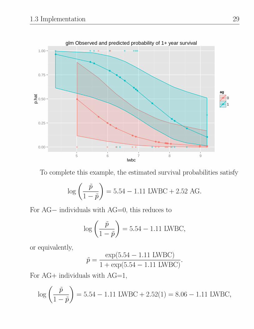
The plot from our Fisher’s Scoring method above is the same as the
plot below from the glm() procedure.
1.3 Implementation 29
●
●●
●
●
●●
●
●
●
●
●●
●
●●
●
●
●
●
●●
● ● ●●● ●● ●0.00
0.25
0.50
0.75
1.00
5 6 7 8 9lwbc
p.ha
t ag
●
●
0
1
glm Observed and predicted probability of 1+ year survival
To complete this example, the estimated survival probabilities satisfy
log
(p
1− p
)= 5.54− 1.11 LWBC + 2.52 AG.
For AG− individuals with AG=0, this reduces to
log
(p
1− p
)= 5.54− 1.11 LWBC,
or equivalently,
p =exp(5.54− 1.11 LWBC)
1 + exp(5.54− 1.11 LWBC).
For AG+ individuals with AG=1,
log
(p
1− p
)= 5.54− 1.11 LWBC + 2.52(1) = 8.06− 1.11 LWBC,

30 Logistic Regression and Newton-Raphson
or
p =exp(8.06− 1.11 LWBC)
1 + exp(8.06− 1.11 LWBC).
Although the equal slopes model appears to fit well, a more general
model might fit better. A natural generalization here would be to add an
interaction, or product term, AG ∗ LWBC to the model. The logistic
model with an AG effect and the AG ∗ LWBC interaction is equivalent
to fitting separate logistic regression lines to the two AG groups. This
interaction model provides an easy way to test whether the slopes are
equal across AG levels. I will note that the interaction term is not needed
here.


