Newton Raphson
38
Principles of Linear Algebra With Maple TM The Newton–Raphson Method Kenneth Shiskowski and Karl Frinkle c Draft date July 26, 2010
-
Upload
rafael-rguez-s -
Category
Documents
-
view
130 -
download
1
Transcript of Newton Raphson

Principles of Linear Algebra With MapleTM
The Newton–Raphson Method
Kenneth Shiskowski and Karl Frinkle
c© Draft date July 26, 2010

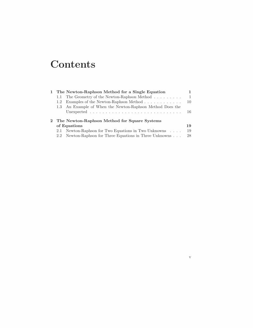
Contents
1 The Newton-Raphson Method for a Single Equation 1
1.1 The Geometry of the Newton-Raphson Method . . . . . . . . . 11.2 Examples of the Newton-Raphson Method . . . . . . . . . . . . 101.3 An Example of When the Newton-Raphson Method Does the
Unexpected . . . . . . . . . . . . . . . . . . . . . . . . . . . . . 16
2 The Newton-Raphson Method for Square Systems
of Equations 19
2.1 Newton-Raphson for Two Equations in Two Unknowns . . . . 192.2 Newton-Raphson for Three Equations in Three Unknowns . . . 28
v

Chapter 1
The Newton-Raphson
Method for a Single
Equation
1.1 The Geometry of the Newton-Raphson
Method
In studying astronomy, Sir Isaac Newton needed to solve an equation f(x) = 0involving trigonometric functions such as sine. He could not do it by anyalgebra he knew and all he really needed was just a very good approximationto the equation’s solution. He then discovered the basic algorithm called theNewton-Raphson Method although Newton found it in a purely algebraic formatwhich was very difficult to use and understand. The general method and itsgeometric basis was actually first seen by Joseph Raphson (1648 - 1715) uponreading Newton’s work although Raphson only used it on polynomial equationsto find their real roots.
The Newton-Raphson method is the true bridge between algebra (solvingequations of the form f(x) = 0 and factoring) and geometry (finding tangentlines to the graph of y = f(x)). What follows will explore the idea of theNewton-Raphson Method and how tangent lines will help us solve equationsboth quickly and easily although not for exact solutions, only approximateones.
The reason that we are studying the Newton-Raphson Method in this bookis that it can also solve square non-linear systems of equations using matricesand their inverses as we shall see later. It is part of the wonderful effectivenessof the Newton-Raphson Method in that it can solve either a single equationor a square system of equations for its real or complex solutions, but only
1
2 Chapter 1. Newton-Raphson Method for a Single Equation
approximately although to as many decimal places as you want.Now we will discuss the important application of using tangent lines to solve
a single equation of the form f(x) = 0 for approximate solutions either real orcomplex.
Example 1.1.1. The best way to understand the simplicity of this methodand its geometric basis is to look at an example. Let’s say that we want tosolve the equation
x3 − 5x2 + 3x+ 5 = 0 (1.1)
for an approximate solution x. We can easily estimate where the real solutionsare by finding the x-intercepts of the graph of y = x3−5x2+3x+5. Rememberthat the total number of real or complex roots to any polynomial is its degree(or order) which in this case is three. Also, when a polynomial has all realcoefficients as this one does all of the complex roots (if there are any) occurin complex conjugate pairs. This particular polynomial has exactly three realroots and no complex roots by looking at its graph below.
> with(plots): with(plottools):
> f:= x -> xˆ3 - 5*xˆ2 + 3*x + 5:
> roots f:= [fsolve(f(x), x, complex)];
roots f := [−0.7092753594, 1.806063434, 3.903211926]
> plot xintercepts:= seq(circle([roots f[j],0], .3, color = blue), j=1..3):
> plotf:= plot(f(x), x = -3..7, thickness = 2):
> display({plotf, plot xintercepts}, view = [-3..7,-4..6]);
–4
–2
2
4
6
y
–2 2 4 6x
Figure 1.1: The three roots of the polynomial x3 − 5x2 + 3x + 5 are its threex-intercepts (circled)
1.1 Geometry of the Newton-Raphson Method 3
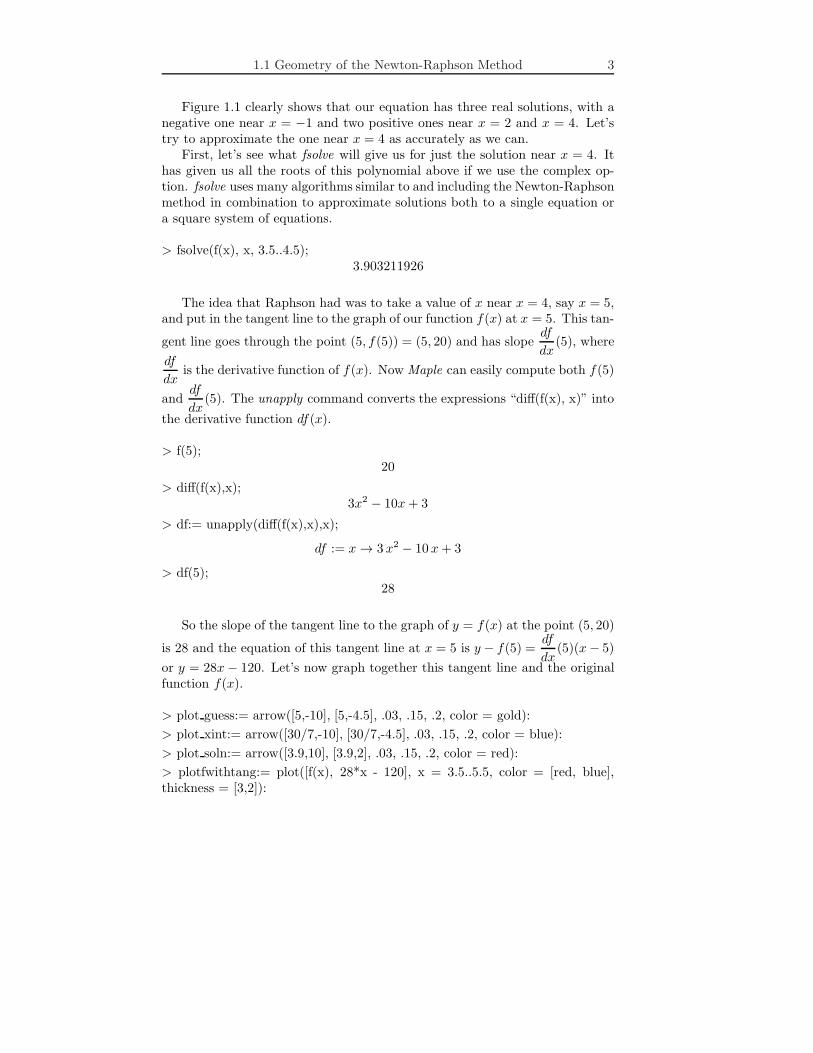
Figure 1.1 clearly shows that our equation has three real solutions, with anegative one near x = −1 and two positive ones near x = 2 and x = 4. Let’stry to approximate the one near x = 4 as accurately as we can.
First, let’s see what fsolve will give us for just the solution near x = 4. Ithas given us all the roots of this polynomial above if we use the complex op-tion. fsolve uses many algorithms similar to and including the Newton-Raphsonmethod in combination to approximate solutions both to a single equation ora square system of equations.
> fsolve(f(x), x, 3.5..4.5);3.903211926
The idea that Raphson had was to take a value of x near x = 4, say x = 5,and put in the tangent line to the graph of our function f(x) at x = 5. This tan-
gent line goes through the point (5, f(5)) = (5, 20) and has slopedf
dx(5), where
df
dxis the derivative function of f(x). Now Maple can easily compute both f(5)
anddf
dx(5). The unapply command converts the expressions “diff(f(x), x)” into
the derivative function df(x).
> f(5);20
> diff(f(x),x);3x2 − 10x+ 3
> df:= unapply(diff(f(x),x),x);
df := x → 3 x2 − 10 x+ 3
> df(5);28
So the slope of the tangent line to the graph of y = f(x) at the point (5, 20)
is 28 and the equation of this tangent line at x = 5 is y − f(5) =df
dx(5)(x− 5)
or y = 28x− 120. Let’s now graph together this tangent line and the originalfunction f(x).
> plot guess:= arrow([5,-10], [5,-4.5], .03, .15, .2, color = gold):
> plot xint:= arrow([30/7,-10], [30/7,-4.5], .03, .15, .2, color = blue):
> plot soln:= arrow([3.9,10], [3.9,2], .03, .15, .2, color = red):
> plotfwithtang:= plot([f(x), 28*x - 120], x = 3.5..5.5, color = [red, blue],thickness = [3,2]):
4 Chapter 1. Newton-Raphson Method for a Single Equation
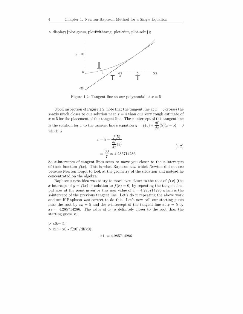
> display({plot guess, plotfwithtang, plot xint, plot soln});
–20
0
20y
4 4.5 5 5.5x
Figure 1.2: Tangent line to our polynomial at x = 5
Upon inspection of Figure 1.2, note that the tangent line at x = 5 crosses thex-axis much closer to our solution near x = 4 than our very rough estimate ofx = 5 for the placement of this tangent line. The x-intercept of this tangent line
is the solution for x to the tangent line’s equation y = f(5)+df
dx(5)(x− 5) = 0
which is
x = 5− f(5)
df
dx(5)
=30
7≈ 4.285714286
(1.2)
So x-intercepts of tangent lines seem to move you closer to the x-interceptsof their function f(x). This is what Raphson saw which Newton did not seebecause Newton forgot to look at the geometry of the situation and instead heconcentrated on the algebra.
Raphson’s next idea was to try to move even closer to the root of f(x) (thex-intercept of y = f(x) or solution to f(x) = 0) by repeating the tangent line,but now at the point given by this new value of x = 4.285714286 which is thex-intercept of the previous tangent line. Let’s do it repeating the above workand see if Raphson was correct to do this. Let’s now call our starting guessnear the root by x0 = 5 and the x-intercept of the tangent line at x = 5 byx1 = 4.285714286. The value of x1 is definitely closer to the root than thestarting guess x0.
> x0:= 5.:
> x1:= x0 - f(x0)/df(x0);
x1 := 4.285714286
1.1 Geometry of the Newton-Raphson Method 5
> f(x1);
4.73760934
> df(x1);
15.24489796
> f(x1) - x1*df(x1);
−60.59766764
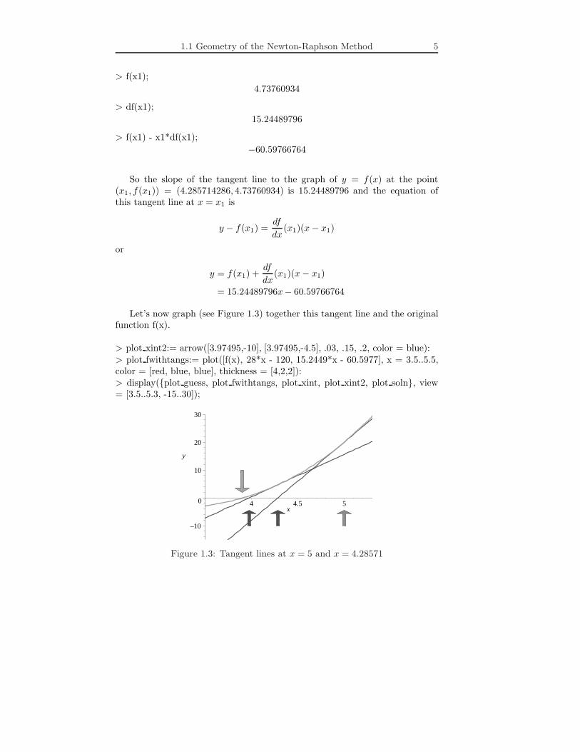
So the slope of the tangent line to the graph of y = f(x) at the point(x1, f(x1)) = (4.285714286, 4.73760934) is 15.24489796 and the equation ofthis tangent line at x = x1 is
y − f(x1) =df
dx(x1)(x− x1)
or
y = f(x1) +df
dx(x1)(x − x1)
= 15.24489796x− 60.59766764
Let’s now graph (see Figure 1.3) together this tangent line and the originalfunction f(x).
> plot xint2:= arrow([3.97495,-10], [3.97495,-4.5], .03, .15, .2, color = blue):> plot fwithtangs:= plot([f(x), 28*x - 120, 15.2449*x - 60.5977], x = 3.5..5.5,color = [red, blue, blue], thickness = [4,2,2]):> display({plot guess, plot fwithtangs, plot xint, plot xint2, plot soln}, view= [3.5..5.3, -15..30]);
–10
0
10
20
30
y
4 4.5 5x
Figure 1.3: Tangent lines at x = 5 and x = 4.28571

6 Chapter 1. Newton-Raphson Method for a Single Equation
Raphson clearly has a very good idea in the use of tangent lines to approxi-mately solve single equations of the form f(x) = 0 if our picture above is trulycorrect. Happily for both Raphson and us, this picture is right and successivetangent lines and their x-intercepts do move closer and closer to the x-interceptof their underlying function f(x).
The general formula for the x-intercept of the tangent line to the graph ofy = f(x) at the point where x = a is
x = a− f(a)
df
dx(a)
, (1.3)
since the equation of the tangent line at x = a is
y = f(a) +df
dx(a)(x − a)
If you now solve
f(a) +df
dx(a)(x− a) = 0
for x, you will get equation (1.3).Let’s use this formula below to get the successive x-intercepts for these
tangent lines. The values of these x-intercepts are clearly moving towards theroot of our polynomial which is roughly at x = 3.9 on the x-axis below the redarrow in the above plots.
The number of digits is now set to twelve instead of the default of ten sincewe want to get ten accurate digits when we round down to ten.
> Digits:= 12:
> x0:= 5.:
> x1:= x0 - f(x0)/df(x0);
x1 := 4.28571428571
> x2:= x1 - f(x1)/df(x1);
x2 := 3.97494740867
> x3:= x2 - f(x2)/df(x2);
x3 := 3.90652292594
> x4:= x3 - f(x3)/df(x3);
x4 := 3.90321950278

1.1 Geometry of the Newton-Raphson Method 7
> x5:= x4 - f(x4)/df(x4);
x5 := 3.90321192597
> x6:= x5 - f(x5)/df(x5);
x6 := 3.90321192590
> x7:= x6 - f(x6)/df(x6);
x7 := 3.90321192592
This is the answer accurate to ten decimal places that fsolve gave us ofx = 3.903211926. We perhaps got it the same way fsolve did since the Newton-Raphson Method is part of fsolve. To get this answer accurate to ten decimalplaces, it took only six repeated applications of the Newton-Raphson Method.This is a very fast procedure even when our starting guess of x = 5 is not veryclose to the root nearest to it.
It should be noted that you stop the Newton-Raphson Method when youget a repetition in the value for two consecutive x-intercepts of your tangentlines accurate to the number of digits you desire. This is the reason we couldcould stop after we got x6 since x6 = x5 accurate to ten digits.
Newton’s Method will in general solve equations of the form f(x) = 0 forthe solution nearest a starting estimate of x = x0. It then creates a list ofvalues xn where each xn (the nth element of this list) is the x-intercept of thetangent line to y = f(x) at the previous list value of x = xn−1. This gives thegeneral formula for the xn of
xn+1 = xn − f(xn)
df
dx(xn)
(1.4)
starting with x0. Each xn is usually closer to being a solution to f(x) = 0 thanthe previous xn−1. The xn can all be gotten from iterating the starting guessx0 in the iteration function
g(x) = x− f(x)
df
dx(x)
(1.5)
This means that xn+1 = g(xn) for all n starting with 0.The method we are using is called iteration since it begins with a starting
guess value of x0 and then finds the iteration values x1, x2, . . . thereafter using
8 Chapter 1. Newton-Raphson Method for a Single Equation
the same formula g(x) based on the previous value. The function g(x) whichcomputes these iteration values is called the iterator.
The following procedure will table some values of this Newton sequenceof iterates from Example 1.1.1 and x0’s near our three solutions which youmust provide as x0. We will carry out n = 8 iterations of the Newton-RaphsonMethod to generate the list of lists called newton. Try different list of values forx0 to see how they affect the Newton list moving toward the solutions nearestthem. The starting list for x0 below was chosen from the graphs above sothat the tangents at these points will intersect the x-axis towards the solutionnearest it. We stop iterating with the iterator g(x) when two consecutive valuesin the sequence of xn’s are the same to the accuracy desired.
We will use the three starting guesses for x0 of 0, 1, and 5 or the list [0., 1., 5.]where the decimal point is used to tell Maple that we want decimal approxima-tions and not exact values since to Maple any number with a decimal point init is considered an approximation. Without these decimal points Maple wouldcompute exact values giving us horrendous fractions for the values of our iter-ates instead of decimal approximations.
> Digits:= 12:
> f:= x -> xˆ3 - 5*xˆ2 + 3*x + 5:
> df:= unapply(diff(f(x),x), x);
df := x → 3x2 − 10x+ 3
> x0:= [0., 1., 5.]:
> n := 8:
> g := unapply(x - f(x)/df(x), x);
g := x → x− x3 − 5 x2 + 3 x+ 5
3 x2 − 10 x+ 3
> newt:= proc(i) map(g, newt(i-1)) end:
> newt(1):= x0:
> newton:= [seq(newt(i), i = 1..n+1)];
[ [0.0, 1.0, 5.0], [−1.66666666667, 2.0, 4.28571428571], [−1.00529100529,
1.80000000000, 3.97494740867], [−0.751331029986, 1.80606060606,
3.90652292594], [−0.710320317972, 1.80606343352, 3.90321950278],
[−0.709276029619, 1.80606343353, 3.90321192597], [−0.709275359437,
1.80606343355, 3.90321192590], [−0.709275359437, 1.80606343352,
3.90321192592], [−0.709275359437, 1.80606343353, 3.90321192589] ]
1.1 Geometry of the Newton-Raphson Method 9
> evalf(fsolve(f(x),x,complex),10);
−0.7092753594, 1.806063434, 3.903211926
> evalf(newton[9],10);
[−0.7092753594, 1.806063434, 3.903211926]
The evalf command has rounded the values in the list newton[9] to tendigits and it agrees to ten digits the results from fsolve. You have just seen theNewton-Raphson Method solve for the three real roots of our polynomial f(x)simultaneously working on finding each root based on three different startingguesses near them.
The next section will continue looking at more examples of the uses of theNewton-Raphson algorithm. It will look for complex roots to polynomials,solve for thirteenth roots of numbers, find inverse trignometric function values.
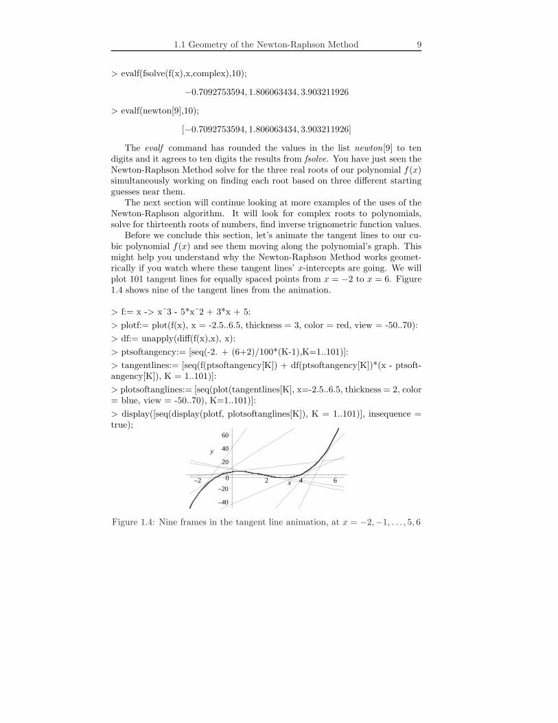
Before we conclude this section, let’s animate the tangent lines to our cu-bic polynomial f(x) and see them moving along the polynomial’s graph. Thismight help you understand why the Newton-Raphson Method works geomet-rically if you watch where these tangent lines’ x-intercepts are going. We willplot 101 tangent lines for equally spaced points from x = −2 to x = 6. Figure1.4 shows nine of the tangent lines from the animation.
> f:= x -> xˆ3 - 5*xˆ2 + 3*x + 5:
> plotf:= plot(f(x), x = -2.5..6.5, thickness = 3, color = red, view = -50..70):
> df:= unapply(diff(f(x),x), x):
> ptsoftangency:= [seq(-2. + (6+2)/100*(K-1),K=1..101)]:
> tangentlines:= [seq(f(ptsoftangency[K]) + df(ptsoftangency[K])*(x - ptsoft-angency[K]), K = 1..101)]:
> plotsoftanglines:= [seq(plot(tangentlines[K], x=-2.5..6.5, thickness = 2, color= blue, view = -50..70), K=1..101)]:
> display([seq(display(plotf, plotsoftanglines[K]), K = 1..101)], insequence =true);
–40
–20
0
20
40
60
y
–2 2 4 6x
Figure 1.4: Nine frames in the tangent line animation, at x = −2,−1, . . . , 5, 6
10 Chapter 1. Newton-Raphson Method for a Single Equation
1.2 Examples of the Newton-Raphson Method
In this section, we will use the machinery developed in Section 1.1, we willapply the Newton-Raphson Method to specific problems.
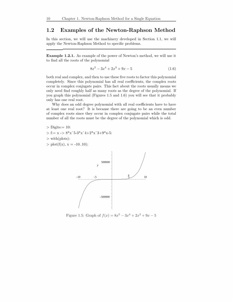
Example 1.2.1. As example of the power of Newton’s method, we will use itto find all the roots of the polynomial
8x5 − 3x4 + 2x3 + 9x− 5 (1.6)
both real and complex, and then to use these five roots to factor this polynomialcompletely. Since this polynomial has all real coefficients, the complex rootsoccur in complex conjugate pairs. This fact about the roots usually means weonly need find roughly half as many roots as the degree of the polynomial. Ifyou graph this polynomial (Figures 1.5 and 1.6) you will see that it probablyonly has one real root.
Why does an odd degree polynomial with all real coefficients have to haveat least one real root? It is because there are going to be an even numberof complex roots since they occur in complex conjugate pairs while the totalnumber of all the roots must be the degree of the polynomial which is odd.
> Digits:= 10:
> f:= x -> 8*xˆ5-3*xˆ4+2*xˆ3+9*x-5:
> with(plots):
> plot(f(x), x = -10..10);
–500000
500000y
–10 –5 5 10x
Figure 1.5: Graph of f(x) = 8x5 − 3x4 + 2x3 + 9x− 5

1.2 Examples of the Newton-Raphson Method 11
> plot(f(x), x = -3..3);
–2000
–1000
0
1000y
–3 –2 –1 1 2 3x
Figure 1.6: Graph of f(x) = 8x5 − 3x4 + 2x3 + 9x− 5
> df:= unapply(diff(f(x),x),x);
df := x → 40x4 − 12x3 + 6x2 + 9
> x0:= [1., 1.+I, -1.-I]:
> g:= unapply(x - f(x)/df(x), x);
g := x → x− 8 x5 − 3 x4 + 2 x3 + 9 x− 5
40 x4 − 12 x3 + 6 x2 + 9
> newt:= proc(i) map(g, newt(i-1)) end:
> newt(1):= x0:
> n:= 8:
> newton:= [seq(newt(i), i = 1..8)];
newton := [ [1., 1.+ 1.I,−1.− 1.I], [0.7441860465, 0.8299022921
+ 0.8664659252I,−0.8350302309− 0.8574919332I], [0.5697030175,
0.7080864702+ 0.8082690821I,−0.7475807128− 0.7820854080I],
[0.5186129098, 0.6518047690+ 0.8166926208I,−0.7231360472
− 0.7605178310I], [0.5161116670, 0.6507190475+ 0.8253549920I,
− 0.7214092342− 0.7588957152I], [0.5161066849, 0.6508476751
+ 0.8252171251I,−0.7214010980− 0.7588870360I], [0.5161066849,
0.6508477553+ 0.8252171632I,−0.7214010978− 0.7588870357I],
[0.5161066849, 0.6508477553+ 0.8252171633I,−0.7214010978
− 0.7588870357I] ]

12 Chapter 1. Newton-Raphson Method for a Single Equation
> rootsf:= [op({op(newton[8]), op(map(conjugate, newton[8]))})];
rootsf := [0.5161066849,−0.7214010978− 0.7588870357I,−0.7214010978
+ 0.7588870357I, 0.6508477553− 0.8252171633I, 0.6508477553
+ 0.8252171633I]
> p:= coeff(f(x),xˆ5)*mul(x-rootsf[j], j=1..5);
p := 8(x− 0.5161066849)(x+ 0.7214010978+ 0.7588870357I)×(x+ 0.7214010978− 0.7588870357I)(x− 0.6508477553+
0.8252171633I)(x− 0.6508477553− 0.8252171633I)
> expand(p);
8x5 − 2.999999999x4 + (8. 10−10I)x+ 1.999999999x3 − 1.6 10−9x2
+ 9.000000000x− 4.999999998+ 4.159135129 10−10)I
> f(x);8x5 − 3x4 + 2x3 + 9x− 5
> factor(f(x),complex);
8.(x + 0.7214010978+ 0.7588870357I)(x+ 0.7214010978− 0.7588870357I)×(x − 0.5161066849)(x− 0.6508477554+ 0.8252171634I)×(x − 0.6508477554− 0.8252171634I)
The polynomial p above gives the complete factoring of f(x) using theroots found from Newton’s method. When we expand p we do not get f(x)back exactly, but we are very close to it due to rounding error in our roots. Thefactor command in Maple using the complex option will factor the polynomialcompletely also.
Example 1.2.2. Now let’s use the Newton-Raphson Method to solve the equa-tion
ex = cos(2x) + 5 (1.7)
for its single real solution where we actually solve
f(x) = ex − cos(2x)− 5 = 0
We will get that the solution is x = 1.400545514 after five iterations startingwith x0 = 2. In order to see where the solution to this equation lies, we will ploteach side of the equation separately and find their intersection point (Figure1.7).
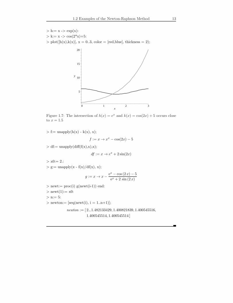
1.2 Examples of the Newton-Raphson Method 13
> h:= x -> exp(x):
> k:= x -> cos(2*x)+5:
> plot([h(x),k(x)], x = 0..3, color = [red,blue], thickness = 2);
5
10
15
20
y
0 1 2 3x
Figure 1.7: The intersection of h(x) = ex and k(x) = cos(2x) + 5 occurs closeto x = 1.5
> f:= unapply(h(x) - k(x), x);
f := x → xx − cos(2x)− 5
> df:= unapply(diff(f(x),x),x);
df := x → ex + 2 sin(2x)
> x0:= 2.:
> g:= unapply(x - f(x)/df(x), x);
g := x → x− ex − cos (2 x)− 5
ex + 2 sin (2 x)
> newt:= proc(i) g(newt(i-1)) end:
> newt(1):= x0:
> n:= 5:
> newton:= [seq(newt(i), i = 1..n+1)];
newton := [ 2., 1.482133429, 1.400821839, 1.400545516,
1.400545514, 1.400545514 ]
14 Chapter 1. Newton-Raphson Method for a Single Equation
Example 1.2.3. As our next example of the Newton-Raphson Method, weuse it to find arctan(1.26195) from the function tan(x) alone. If we let x =arctan(1.26195), then by taking tangent of both sides we have
tan(x) = tan(arctan(1.26195)) = 1.26195
Now rewriting this as f(x) = tan(x)− 1.26195 = 0, we have our function f(x)
which has the arctan(1.26195) as root. Since arctan(z) is always between −π
2and
π
2, we let x0 = 1 because if z > 0, then arctan(z) > 0. Using twelve digits,
the end result of the Newton-Raphson Method should be accurate to ten digits.
> Digits:= 12:
> f:= x -> tan(x) - 1.26195:
> df:= unapply(diff(f(x),x),x);
df := x → 1 + tan(x)2
> x0:= 1.:
> g:= unapply(x - f(x)/df(x), x);
g := x → x− tan (x)− 1.26195
1 + (tan (x))2
> newt:= proc(i) g(newt(i-1)) end:
> newt(1):= x0:
> n:= 5:
> newton:= [seq(newt(i), i = 1..6)];
newton := [ 1., 0.913748036398, 0.900908331438, 0.900691798443,
0.900691739234, 0.900691739234 ]
> evalf(newton[6],10);0.9006917392
> evalf(arctan(1.26195),10);
0.9006917392
1.2 Examples of the Newton-Raphson Method 15
Example 1.2.4. As the last example of this section, we use the Method tofind
13√8319407225, or 83194072251/13. This thirteenth root can be found by
letting x = 83194072251/13 and then rewriting this equation without the rootas
x13 − 8319407225 = 0 (1.8)
We then havef(x) = x13 − 8319407225 = 0 (1.9)
Now we have our function f(x) for the Method. Since
513 = 1220703125< 8319407225 < 13060694016 = 613
we can take the starting guess to be either x0 = 5 or x0 = 6 since we usuallychoose an integer for the starting value x0 (although not required). You couldalso plot y = f(x) and look for the x-intercept of this graph.
> 5ˆ13;1220703125
> 6ˆ13;13060694016
> f:= x -> xˆ13-8319407225:
> df:= unapply(diff(f(x),x),x);
df := x → 13 x12
> x0:= 6.:
> g:= unapply(x - f(x)/df(x), x);
g := x → x− 1
13
x13 − 8319407225
x12
> newt:= proc(i) g(newt(i-1)) end:
> newt(1):= x0:
> n:= 5:
> newton:= [seq(newt(i), i = 1..n+1)];
newton := [ 6., 5.83245253211, 5.79678752512, 5.79541014785,
5.79540818028, 5.79540818028 ]
> evalf(newton[6],10);5.795408180
> evalf(8319407225ˆ(1/13),10);
5.795408180

16 Chapter 1. Newton-Raphson Method for a Single Equation
These last two examples of the Method illustrate that it can be used tofind the values of inverse trignometric functions using the regular trignometricfunctions and to get roots of numbers using powers. It can also find the valuesof logarithms using exponentials. The Method also has a version which allowsyou to solve square systems of non-linear equations.
1.3 An Example of When the Newton-Raphson
Method Does the Unexpected
The next example of the Method will show you that if you start with an x0
which isn’t very good, then you may slowly move towards a solution of f(x) = 0,but not the nearest one to where you started.
Example 1.3.1. Let’s solve the trigonometric equation sin(x) = 0 with astarting value of x0 = 1.97603146838. You should expect that we will get thevalue of π using the Method. The graph of sin(x) is given in Figure 1.8 below.
> Digits:= 12:
> f:= x -> sin(x):
> plot(f(x), x=0..2*Pi);
–1
–0.5
0
0.5
1
y
2 4 6x
Figure 1.8: Graph of f(x) = sin(x) on the interval [0, 2π]
> n:= 20:
> x0:= 1.97603146838:
> df:= unapply(diff(f(x),x),x);
df := x → cos(x)
> g:= unapply(x - f(x)/df(x), x);
g :=→ x− sin(x)
cos(x)
1.3 When the Newton-Raphson Method Does the Unexpected 17
> newt:= proc(i) evalf(g(newt(i-1))) end:
> newt(1):= x0;newt(1) := 1.97603146838
> newton:= [seq(newt(i), i = 1..n+1)];
newton := [ 1.97603146838, 4.30715383881, 1.97603146831, 4.30715383919,
1.97603146625, 4.30715385038, 1.97603140544, 4.30715418084,
1.97602960967, 4.30716393934, 1.97597657917, 4.30745215919,
1.97440902034, 4.31601007571, 1.92670276467, 4.61678041455,
− 5.81064450865,−6.32181094255,−6.28316608667,
− 6.28318530718,−6.28318530718 ]
> evalf(-2*Pi,12);−6.28318530718
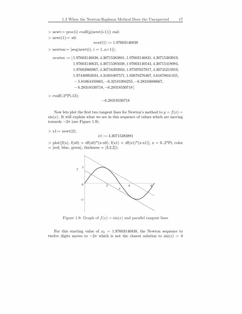
Now lets plot the first two tangent lines for Newton’s method to y = f(x) =sin(x). It will explain what we see in this sequence of values which are movingtowards −2π (see Figure 1.9).
> x1:= newt(2);x1 := 4.30715383881
> plot([f(x), f(x0) + df(x0)*(x-x0), f(x1) + df(x1)*(x-x1)], x = 0..2*Pi, color= [red, blue, green], thickness = [3,2,2]);
–1
0
1y
2 4 6x
Figure 1.9: Graph of f(x) = sin(x) and parallel tangent lines
For this starting value of x0 = 1.97603146838, the Newton sequence totwelve digits moves to −2π which is not the closest solution to sin(x) = 0
18 Chapter 1. Newton-Raphson Method for a Single Equation
to x0, which is π. The values in this sequence approximately alternate eachother for a long time until suddenly they move off towards −2π. They do thisbecause the tangent lines used in the Method are approximately parallel lineswhere each has x-intercept approximately the x-coordinate value of the other.You should see what happens to this sequence of iterates if you increase thenumber of digits to sixteen.
The Newton-Raphson Method works quickly to give very good accuracy.It normally takes no more than five to ten iterations from a reasonable initialguess x0 to get the solution accurate to ten or more decimal places. Eachiteration usually produces greater accuracy, and you reach the accuracy youwant when two consecutive iterations agree in value to this accuracy.

Chapter 2
The Newton-Raphson
Method for Square Systems
of Equations
2.1 Newton-Raphson for Two Equations in Two
Unknowns
In this section we will discuss the Newton-Raphson method for solving square(as many equations as variables) systems of two non-linear equations
f(x, y) = 0, g(x, y) = 0
in the two variables x and y. In order to do this we must combine these twoequations into a single equation of the form F (x, y) = 0 where F must give usa two component column vector and 0 is also the two component zero columnvector, that is,
F (x, y) =
[
f(x, y)g(x, y)
]
(2.1)
and 0 =
[
00
]
. Then clearly the equation F (x, y) = 0 is the same as
[
f(x, y)g(x, y)
]
=
[
00
]
(2.2)
which is equivalent to the system of two equations f(x, y) = 0 and g(x, y) = 0.Now let F : R2 → R
2 be a continuous function which has continuous firstpartial derivatives where F is defined as in equation (2.1) for variables x, y andcomponent functions f(x, y), g(x, y). We wish to solve the equation F (x, y) =
19

20 Chapter 2. Newton-Raphson Method for Square Systems
0 which is really solving simultaneously the square system of two non-linearequations given by f(x, y) = 0 and g(x, y) = 0.
In order to do this, we shall have to generalize the one variable Newton-Raphson method iterator formula for solving the equation f(x) = 0 given bythe sequence pk for p0 the starting guess where
pk+1 = pk − f(pk)
df
dx(pk)
(2.3)
orpk+1 = g(pk)
where
g(pk) = pk −f(pk)
df
dx(pk)
(2.4)
is the (single equation) Newton-Raphson iterator.To see how this can be done, you must realize that now in the two equation
case that
p0 =
[
x0
y0
]
(2.5)
is our starting guess as a point in the xy-plane written as a column vector,
pk =
[
xk
yk
]
(2.6)
is the kth iteration of our method, and
F (pk) =
[
f(xk, yk)g(xk, yk)
]
are all two component column vectors in R2 and not numbers as in the single
variable case. Thus, dividing a two component column vector by a derivativerequires that we be dividing by a 2 × 2 matrix, or multiplying by the inverse
of this matrix. Thus, we need to replacedf
dxin our old iterator g(x) by a 2× 2
matrix consisting of the four partial derivatives of F (x, y), which are∂f
∂x,∂f
∂y,
∂g
∂x, and
∂g
∂y.
The choice of this new derivative matrix is the 2×2 Jacobian matrix J(x, y),of F(x,y), given by the 2× 2 matrix
J(x, y) =
∂f
∂x
∂f
∂y
∂g
∂x
∂g
∂y
(2.7)
2.1 Newton-Raphson for Two Equations in Two Unknowns 21
Other choices for this 2 × 2 matrix of partial derivatives are possible and youshould see if they will also work in place of this Jacobian matrix, but thisJacobian matrix seems most logical if you think about the fact that for F (x, y),the first row is f(x, y) and g(x, y) is in the second row while the variables aregiven as x first and y second in all these functions. Thus, the Newton-Raphsonarray (list or sequence) is now for a starting vector p0, as defined in equation(2.5), given by
pk+1 = pk − (J(pk))−1
F (pk) (2.8)
where the vector F (pk) is multiplied on its left by the inverse of the Jacobianmatrix J(x, y) evaluated at pk, i.e., J(pk) = J(xk, yk).
Note that finding (J(pk))−1
in each iteration is a formidable task if thesystem of equations is large, say 25× 25 or more, and so at each iteration youcan instead solve for pk+1 by solving the square linear system of equations
J(pk) pk+1 = J(pk) pk − F (pk)
where the components of pk+1 are the unknowns. Of course, it is easy to findpk+1 directly if you are in a small number of equations case such as ours usingthe inverse matrix.
Example 2.1.1. Let F : R2 → R2 be given in the form of equation (2.1), for
f(x, y) =1
64(x− 11)2 − 1
100(y − 7)2 − 1, g(x, y) = (x − 3)2 + (y − 1)2 − 144
We wish to apply the Newton-Raphson method to solve F (x, y) =
[
00
]
or
equivalently the square system
f(x, y) = 0, g(x, y) = 0
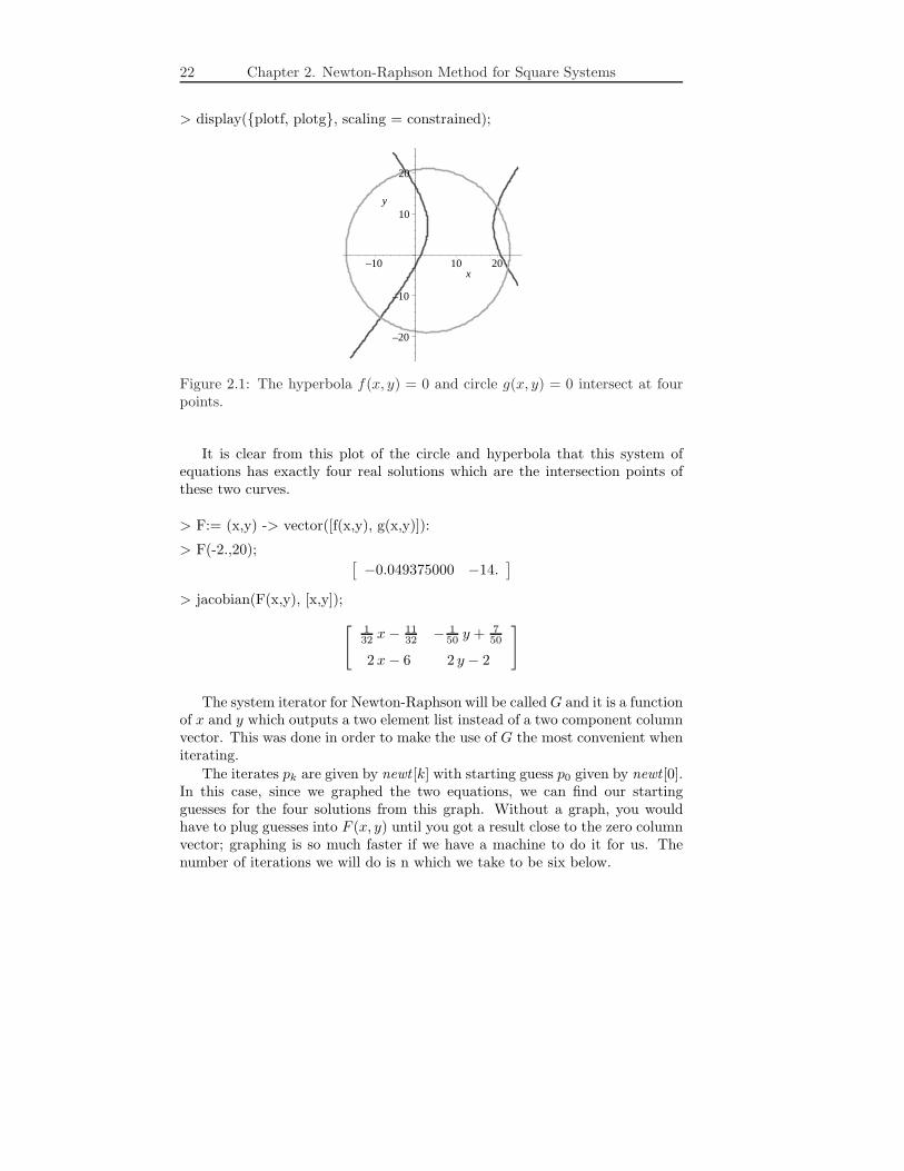
The solutions are the intersection points of these two curves f(x, y) = 0 whichis a hyperbola, and g(x, y) = 0 which is a circle, and is depicted in Figure 2.1.
> with(linalg): with(plots):
> f:= (x,y) -> (x-11)ˆ2/64 - (y-7)ˆ2/100 - 1:
> g:= (x,y) -> (x-3)ˆ2 + (y-1)ˆ2 - 400:
> plotf:= implicitplot(f(x,y) = 0, x = -25..25, y = -25..25, color = blue, grid= [50,50]):
> plotg:= implicitplot(g(x,y) = 0, x = -25..25, y = -25..25, color = red, grid= [50,50]):
22 Chapter 2. Newton-Raphson Method for Square Systems
> display({plotf, plotg}, scaling = constrained);
–20
–10
10
20
y
–10 10 20x
Figure 2.1: The hyperbola f(x, y) = 0 and circle g(x, y) = 0 intersect at fourpoints.
It is clear from this plot of the circle and hyperbola that this system ofequations has exactly four real solutions which are the intersection points ofthese two curves.
> F:= (x,y) -> vector([f(x,y), g(x,y)]):
> F(-2.,20);[
−0.049375000 −14.]
> jacobian(F(x,y), [x,y]);
[
132 x− 11
32 − 150 y +
750
2 x− 6 2 y − 2
]
The system iterator for Newton-Raphson will be calledG and it is a functionof x and y which outputs a two element list instead of a two component columnvector. This was done in order to make the use of G the most convenient wheniterating.
The iterates pk are given by newt [k] with starting guess p0 given by newt [0].In this case, since we graphed the two equations, we can find our startingguesses for the four solutions from this graph. Without a graph, you wouldhave to plug guesses into F (x, y) until you got a result close to the zero columnvector; graphing is so much faster if we have a machine to do it for us. Thenumber of iterations we will do is n which we take to be six below.

2.1 Newton-Raphson for Two Equations in Two Unknowns 23
> G:= unapply(convert(simplify(evalm(vector([x, y]) - jacobian(F(x,y),[x,y])ˆ(-1)&*F(x, y))), list), x, y);
G := (x, y) →[
1
2
41 x2y − 137 x2 + 5599 y− 96 y2 − 43039
41 xy − 137 x− 323 y+ 611,
−1
2
−41 xy2 + 323 y2 + 200 x2 − 10391 x+ 109173
41 xy − 137 x− 323 y+ 611
]
> G(-.25+.433*I,.433-.75*I);
[−35.67946232+ 9.764850390I,−92.91549690+ 40.44912122I]
> n:= 6:> newt[0]:= [-2., 20]:> for i from 1 to n do
newt[i]:= G(newt[i-1][1], newt[i-1][2]);od:
> seq(newt[i-1],i=1..n+1);
[−2., 20], [−2.305821206, 20.28794179], [−2.302041868, 20.28440766],
[−2.302041289, 20.28440713], [−2.302041292, 20.28440712],
[−2.302041294, 20.28440712], [−2.302041294, 20.28440712]
> root1 := newt[6];
root1 := [−2.302041294, 20.28440712]
So the root of the system of equations closest to the point (−2, 20) is newt [6]which we have called root1. We also check this root using fsolve where we musttell it where to look in order to get back just this single root.
After each computation of the table newt we will unassign it so that it iscleared to be used again without worrying that if we change n to a smallervalue we may get leftover values in newt from its previous use. You can clearnewt using the unassign command or by saying “newt:= ‘newt’;”.
> fsolve({f(x,y) = 0, g(x,y) = 0}, {x, y}, {x=-3..0,y=15..25});
{x = −2.302041291, y = 20.28440712}
> unassign(’newt’);
> n:= 7:
> newt[0]:= [20., 13]:
> for i from 1 to n do

24 Chapter 2. Newton-Raphson Method for Square Systems
newt[i]:= G(newt[i-1][1], newt[i-1][2]);od:
> seq(newt[i-1],i=1..n+1);
[20., 13], [19.84349030, 11.84672207], [19.85957225, 11.75930869],
[19.85966012, 11.75880390], [19.85966010, 11.75880388],
[19.85966012, 11.75880390], [19.85966010, 11.75880388],
[19.85966012, 11.75880390]
> root2:= newt[7];
root2 := [19.85966012, 11.75880390]
> unassign(’newt’);
> newt[0]:= [20., -4]:
> newt[0]:= [20., 13]:
> for i from 1 to n donewt[i]:= G(newt[i-1][1], newt[i-1][2]);
od:
> seq(newt[i-1],i=1..n+1);
[20.,−4], [22.75576876,−3.230386204], [22.52089182,−3.359663132],
[22.51902586,−3.359774453], [22.51902576,−3.359774536],
[22.51902576,−3.359774542], [22.51902576,−3.359774539],
[22.51902574,−3.359774540]
> root3:= newt[6];
root3 := [22.51902576,−3.359774539]
> unassign(‘newt’);
> newt[0]:= [-10., -16]:
> for i from 1 to n donewt[i]:= G(newt[i-1][1], newt[i-1][2]);
od:
> seq(newt[i-1],i=1..n+1);
[−10.,−16], [−8.625683855,−15.34506528], [−8.564570385,−15.31763460],
[−8.564449435,−15.31758282], [−8.564449440,−15.31758282],
[−8.564449445,−15.31758282], [−8.564449435,−15.31758282],
[−8.564449440,−15.31758282]
2.1 Newton-Raphson for Two Equations in Two Unknowns 25
> root4:= newt[6];
root4 := [−8.564449435,−15.31758282]
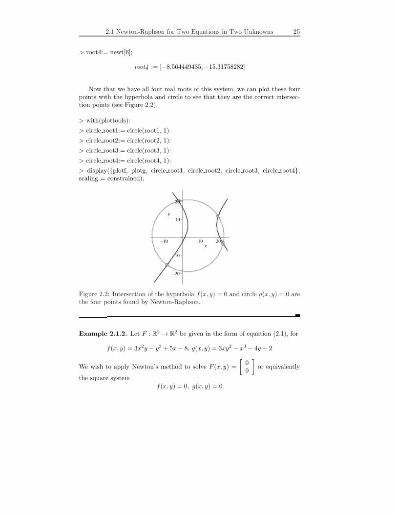
Now that we have all four real roots of this system, we can plot these fourpoints with the hyperbola and circle to see that they are the correct intersec-tion points (see Figure 2.2).
> with(plottools):
> circle root1:= circle(root1, 1):
> circle root2:= circle(root2, 1):
> circle root3:= circle(root3, 1):
> circle root4:= circle(root4, 1):
> display({plotf, plotg, circle root1, circle root2, circle root3, circle root4},scaling = constrained);
–20
–10
10
20
y
–10 10 20x
Figure 2.2: Intersection of the hyperbola f(x, y) = 0 and circle g(x, y) = 0 arethe four points found by Newton-Raphson.
Example 2.1.2. Let F : R2 → R2 be given in the form of equation (2.1), for
f(x, y) = 3x2y − y3 + 5x− 8, g(x, y) = 3xy2 − x3 − 4y + 2
We wish to apply Newton’s method to solve F (x, y) =
[
00
]
or equivalently
the square system
f(x, y) = 0, g(x, y) = 0
26 Chapter 2. Newton-Raphson Method for Square Systems
The real solutions are the real intersection points of these two curves.
> with(linalg): with(plots):
> f:= (x,y) -> 3*xˆ2*y-yˆ3+5*x-8:
> g:= (x,y) -> 3*x*yˆ2-xˆ3-4*y+2:
> plotf:= implicitplot(f(x,y) = 0, x = -10..10, y = -10..10, color = blue, grid= [50,50]):
> plotg:= implicitplot(g(x,y) = 0, x = -10..10, y = -10..10, color = red, grid= [50,50]):
> display({plotf, plotg});
–10
–5
5
10
y
–10 –5 5 10x
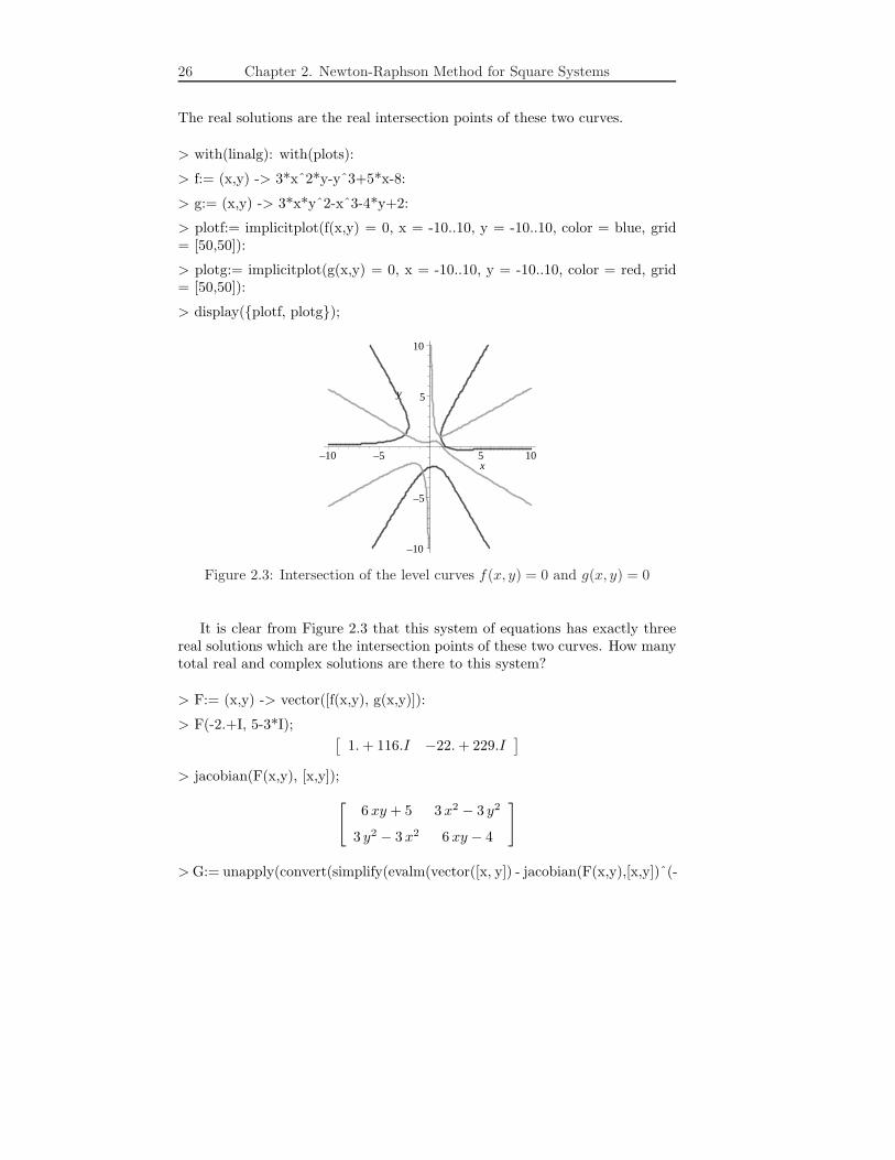
Figure 2.3: Intersection of the level curves f(x, y) = 0 and g(x, y) = 0
It is clear from Figure 2.3 that this system of equations has exactly threereal solutions which are the intersection points of these two curves. How manytotal real and complex solutions are there to this system?
> F:= (x,y) -> vector([f(x,y), g(x,y)]):
> F(-2.+I, 5-3*I);[
1.+ 116.I −22.+ 229.I]
> jacobian(F(x,y), [x,y]);
[
6 xy + 5 3 x2 − 3 y2
3 y2 − 3 x2 6 xy − 4
]
>G:= unapply(convert(simplify(evalm(vector([x, y]) - jacobian(F(x,y),[x,y])ˆ(-

2.1 Newton-Raphson for Two Equations in Two Unknowns 27
1)&*F(x, y))), list), x, y);
G := (x, y) →[
2(
6 x3y2 − 12 x2y + 3 x5 + 3 xy4 + 24 xy + 4 y3 − 16 + 3 x2 − 3 y2)
18 x2y2 + 6 xy − 20 + 9 x4 + 9 y4,
2(
6 x2y3 + 15 xy2 + 3 yx4 + 3 y5 − 5 x3 + 12 x2 − 12 y2 − 6 xy − 5)
18 x2y2 + 6 xy − 20 + 9 x4 + 9 y4
]
> G(-.25+.433*I,.433-.75*I);
[1.067211700− .3138214174I,−0.05450721154− 0.4714997210I
> n:= 12:
> unassign(‘newt’):
> newt[0]:= [7.-10*I, -5+3*I]:
> for i from 1 to n donewt[i]:= G(newt[i-1][1], newt[i-1][2]);
od:
> seq(newt[i-1],i=1..n+1);
[7.− 10.I,−5 + 3I],
[4.716076290− 6.600715228I,−3.382974902+ 2.012179590I],
[3.224169736− 4.308649374I,−2.326626794+ 1.372634953I],
[2.283146120− 2.754133252I,−1.643936873+ 0.9907359528I],
[1.742859710− 1.716145676I,−1.178525033+ 0.8220028622I],
[1.465295509− 1.093767693I,−0.7709379106+ 0.7882814566I],
[1.292418266− 0.7605470184I,−0.3991705530+ 0.7485523402I],
[1.204529252− 0.5825119536I,−0.1451240359+ 0.6817317358I],
[1.196760919− 0.5156573282I,−0.05289160786+ 0.6188832694I],
[1.202567805− 0.5094748562I,−0.04975287894+ 0.6035737078I],
[1.202681506− 0.5095861122I,−0.05002819636+ 0.6035124202I],
[1.202681462− 0.5095860764I,−0.05002810388+ 0.6035124460I],
[1.202681463− 0.5095860762I,−0.05002810432+ 0.6035124462I]
> F(newt[12][1], newt[12][2]);
[
7. 10−9 + 1. 10−9I −2.8 10−9 + 3. 10−9I]
28 Chapter 2. Newton-Raphson Method for Square Systems
This last example indicates that we have at least one complex solution tothis real system of equations.
Conclusions: (1) It should be clear from the above examples that even thesystem of equations version of the Newton-Raphson method is very fast! It alsoworks to generate complex solutions as long as the starting value of newt [0] isalso complex when your equations are real. Redo the above example to see ifyou can find another complex solution. Is the complex conjugate of a solutionin the last example also a solution?
(2) Also, rewrite the code above so that no inverse of the Jacobian is neededsince this is impractical for large matrices and systems of equations.
(3) Now try using the Newton-Raphson method to solve the system
(x − 4)2 + (y − 9)2 = 25, (x− 3)2 + (y − 7)2 = 36
for both solutions. The two real solutions here are the intersection points ofthese two circles. Are there any complex solutions?
2.2 Newton-Raphson for Three Equations in
Three Unknowns
In this section we will look at an example of using the system version of theNewton-Raphson method to solve a 3 × 3 system of equations which are allspheres in space.
Example 2.2.1. Our three spheres have the equations
(x− 5)2 + (y − 9)2 + (z − 4)2 = 49
(x− 2)2 + (y − 7)2 + (z − 13)2 = 100
(x− 6)2 + (y − 11)2 + (z − 10)2 = 64
(2.9)
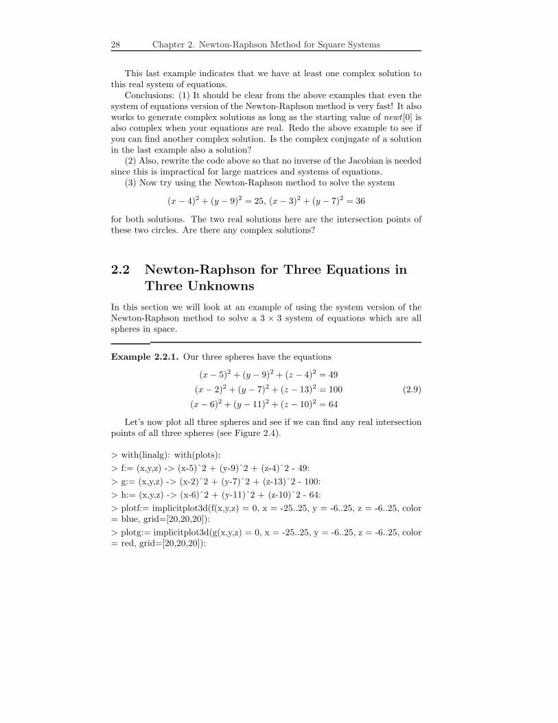
Let’s now plot all three spheres and see if we can find any real intersectionpoints of all three spheres (see Figure 2.4).
> with(linalg): with(plots):
> f:= (x,y,z) -> (x-5)ˆ2 + (y-9)ˆ2 + (z-4)ˆ2 - 49:
> g:= (x,y,z) -> (x-2)ˆ2 + (y-7)ˆ2 + (z-13)ˆ2 - 100:
> h:= (x,y,z) -> (x-6)ˆ2 + (y-11)ˆ2 + (z-10)ˆ2 - 64:
> plotf:= implicitplot3d(f(x,y,z) = 0, x = -25..25, y = -6..25, z = -6..25, color= blue, grid=[20,20,20]):
> plotg:= implicitplot3d(g(x,y,z) = 0, x = -25..25, y = -6..25, z = -6..25, color= red, grid=[20,20,20]):
2.1 Newton-Raphson for Three Equations in Three Unknowns 29
> ploth:= implicitplot3d(h(x,y,z) = 0, x = -25..25, y = -6..25, z = -6..25, color= green, grid=[20,20,20]):
> display({plotf, plotg, ploth}, axes = boxed, scaling = constrained);
–200 10 20x 0 10 20
y
0
10
20
z
Figure 2.4: Intersection of three spheres
It is clear from this plot of the three spheres that this system of equationshas exactly two real solutions which are the intersection points of these threespheres near the points (−2, 14, 6) and (8, 5, 7).
We now use the Newton-Raphson system method to solve our problemwhere F : R3 → R
3 be given by
F (x, y, z) =
f(x, y, z)g(x, y, z)h(x, y, z)
(2.10)
for
f(x, y, z) = (x− 5)2 + (y − 9)2 + (z − 4)2 − 49
g(x, y, z) = (x− 2)2 + (y − 7)2 + (z − 13)2 − 100
h(x, y, z) = (x− 6)2 + (y − 11)2 + (z − 10)2 − 64
(2.11)
We wish to apply the Newton-Raphson method to solve
F (x, y, z) =
000
> F:= (x,y,z) -> vector([f(x,y,z), g(x,y,z), h(x,y,z)]):
> F(-2.,14,6);[
29. 14. 25.]

30 Chapter 2. Newton-Raphson Method for Square Systems
> jacobian(F(x,y,z), [x,y,z]);
2 x− 10 2 y − 18 2 z − 82 x− 4 2 y − 14 2 z − 262 x− 12 2 y − 22 2 z − 20
The system iterator for Newton-Raphson will be calledG and it is a functionof x, y, and z which outputs a three element list instead of a three componentcolumn vector. This was done in order to make the use ofG the most convenientwhen iterating.
The iterates pk are given by newt [k] with starting guess p0 given by newt [0].In this case, since we graphed the three equations, we can find our startingguesses for the two solutions from this graph. Without a graph, you wouldhave to plug guesses into F (x, y, z) until you got a result close to the zero col-umn vector; graphing is so much faster. The number of iterations we will do isn which we take to be seven below.
> G:= unapply(convert(simplify(evalm(vector([x, y, z]) - jacobian(F(x, y, z),[x, y, z])ˆ (-1)&*F(x, y, z))), list), x, y, z);
G := (x, y) →[
3118− 169 z − 393 y+ 15 x2 + 15 y2 + 15 z2
30 x− 27 y + 4 z + 77,
−1
2
−409 z − 786 x+ 27 x2 + 27 y2 + 27 z2 + 3595
30 x− 27 y + 4 z + 77,
1
2
1699 + 338 x− 409 y + 4 x2 + 4 y2 + 4 z2
30 x− 27 y + 4 z + 77
]
> G(-2.,14,6);
[−0.4213649852, 13.47922848, 5.577151335]
> n:= 7:
> newt[0]:= [-2., 14, 6]:
> for i from 1 to n donewt[i]:= G(newt[i-1][1], newt[i-1][2], newt[i-1][3]);
od:
> seq(newt[i-1],i=1..n+1);
[−2., 14, 6],
[−.4213649852, 13.47922848, 5.577151335],
[−.2622019058, 13.33598171, 5.598373075],
[−.2596155823, 13.33365402, 5.598717920],
[−.2596148955, 13.33365340, 5.598718015],

2.1 Newton-Raphson for Three Equations in Three Unknowns 31
[−.2596148984, 13.33365341, 5.598718015],
[−.2596149018, 13.33365340, 5.598718015],
[−.2596148982, 13.33365340, 5.598718015]
> root1 := newt[7];
root1 := [−.2596148982, 13.33365340, 5.598718015]
> F(root1[1], root1[2], root1[3]);
[
−4. 10−8 −1.0 10−7 −3. 10−8]
> fsolve({f(x, y, z) = 0, g(x, y, z) = 0, h(x, y, z)=0}, {x, y, z}, {x=-4..0,y=10..18, z=0..12});
{x = −.2596148966, y = 13.33365341, z = 5.598718014}
So the root of the system of equations closest to the point (−2, 14, 6) isnewt [7] which we have called root1 . We also checked this root in two ways byfirst plugging it back in the function F to see if we get very close to zero (whichwe do) and then by using fsolve where we must tell it where to look in orderto get back just this single root.
After each computation of the table newt we will unassign it so that it iscleared to be used again without worrying that if we change n to a smallervalue we may get leftover values in newt from its previous use. You can clearnewt using the unassign command or by saying “newt:= ‘newt’;”.
> unassign(’newt’);
> n:= 10:
> newt[0]:= [8., 5, 7]:
> for i from 1 to n donewt[i]:= G(newt[i-1][1], newt[i-1][2], newt[i-1][3]);
od:
> seq(newt[i-1],i=1..n+1);
[8., 5, 7],
[9.714285714, 4.357142857, 6.928571430],
[9.533470118, 4.519876898, 6.904462680],
[9.530132750, 4.522880526, 6.904017705],
[9.530131613, 4.522881542, 6.904017550],
[9.530131612, 4.522881554, 6.904017545],

32 Chapter 2. Newton-Raphson Method for Square Systems
[9.530131611, 4.522881541, 6.904017545],
[9.530131612, 4.522881544, 6.904017550],
[9.530131612, 4.522881538, 6.904017550],
[9.530131612, 4.522881536, 6.904017545],
[9.530131612, 4.522881542, 6.904017550]
> root2:= newt[10];
root2 := [9.530131612, 4.522881542, 6.904017550]
> F(root2[1], root2[2], root2[3]);
[
4. 10−8 −3. 10−7 5. 10−8]
> fsolve({f(x,y,z) = 0, g(x,y,z) = 0, h(x,y,z) = 0}, {x, y, z}, {x=5..15, y=0..10,z=0..14});
{x = 9.530131614, y = 4.522881547, z = 6.904017549}
Now we will start with a complex guess to see if our system might have anycomplex solutions.
> unassign(’newt’);
> n:= 10:
> newt[0]:= [15.-20*I, -14+8*I, -50-9*I]:
> for i from 1 to n donewt[i]:= G(newt[i-1][1], newt[i-1][2], newt[i-1][3]);
od:
> seq(newt[i-1],i=1..n+1);
[15.− 20.I,−14 + 8I,−50− 9I], [30.72301499+ 36.44398407I,
− 14.55071349− 32.79958566I, 9.729735330+ 4.859197876I],
[17.83472141+ 18.00464381I,−2.951249272− 16.20417943I,
8.011296190+ 2.400619174I], [11.55226588+ 8.569543596I,
2.702960707− 7.712589245I, 7.173635450+ 1.142605814I],
[8.777004113+ 3.438297071I, 5.200696300− 3.094467366I,
6.803600550+ .4584396097I], [8.418505686+ .2976097941I,
5.523344885− 0.2678488144I, 6.755800760+ 0.03968130744I],
[9.673970474− 0.09876135077I, 4.393426578+ 0.08888521560I,
6.923196065− 0.01316818010I], [9.531271615− 0.002796971041I,

2.1 Newton-Raphson for Three Equations in Three Unknowns 33
4.521855548+ 0.002517273967I, 6.904169550− 0.0003729294942I],
[9.530130955− 6.516297833 10−7I, 4.522882147+ 5.864707365 10−7I,
6.904017460− 8.688510460 10−8I], [9.530131615+ 8.855537408 10−14I,
4.522881549− 7.890932410 10−14I, 6.904017550+ 1.237092006 10−14I],
[9.530131616− 2.761169677 10−23I, 4.522881547+ 3.876817403 10−23I,
6.904017545+ 2.647815558 10−23I]
With this complex starting value we have gotten back to the previous realsolution in root2 since all of the imaginary parts of the solution above are allvery close to zero. You should try more complex starting guesses and see ifthey all give these two real solutions or not. Do you believe that this systemof equations has only two real solutions and no complex ones?