LINEAR ALGEBRA - cool.ntu.edu.tw
179
LINEAR ALGEBRA (Draft) I-Liang Chern National Taiwan University November 9, 2021
Transcript of LINEAR ALGEBRA - cool.ntu.edu.tw

LINEAR ALGEBRA
(Draft)
I-Liang Chern
National Taiwan University
November 9, 2021

2

Contents
1 Vector Spaces 51.1 The Rn space . . . . . . . . . . . . . . . . . . . . . . . . . . . . . . . . . . . 5
1.1.1 Real line and real number system . . . . . . . . . . . . . . . . . . . . 51.1.2 Plane vector and Plane coordinate . . . . . . . . . . . . . . . . . . . 61.1.3 Inner product and Euclidean space . . . . . . . . . . . . . . . . . . . 8
1.2 Subspaces . . . . . . . . . . . . . . . . . . . . . . . . . . . . . . . . . . . . . 121.2.1 Subspaces . . . . . . . . . . . . . . . . . . . . . . . . . . . . . . . . . 121.2.2 Linear Spans and orthogonal complements . . . . . . . . . . . . . . . 141.2.3 Affine Subspaces . . . . . . . . . . . . . . . . . . . . . . . . . . . . . 18
1.3 Linear Independence and Bases . . . . . . . . . . . . . . . . . . . . . . . . . 211.3.1 Linear Independence . . . . . . . . . . . . . . . . . . . . . . . . . . . 211.3.2 Dimensions . . . . . . . . . . . . . . . . . . . . . . . . . . . . . . . . 24
1.4 System of Linear Equations . . . . . . . . . . . . . . . . . . . . . . . . . . . 281.4.1 Setup and matrix notation . . . . . . . . . . . . . . . . . . . . . . . . 281.4.2 Geometric view point of linear equations . . . . . . . . . . . . . . . . 32
1.5 Gaussian elimination . . . . . . . . . . . . . . . . . . . . . . . . . . . . . . . 351.5.1 Elimination as a reduction process . . . . . . . . . . . . . . . . . . . 351.5.2 Solving a linear system in a reduced echelon form . . . . . . . . . . . 431.5.3 Geometric interpretation of the Gaussian elimination . . . . . . . . . 46
1.6 Applications . . . . . . . . . . . . . . . . . . . . . . . . . . . . . . . . . . . . 521.6.1 Polynomial interpolation . . . . . . . . . . . . . . . . . . . . . . . . . 521.6.2 Compatibility condition for solvability . . . . . . . . . . . . . . . . . 561.6.3 Linear systems modeled on graphs . . . . . . . . . . . . . . . . . . . 58
2 Function Spaces 652.1 Abstract Vector Spaces . . . . . . . . . . . . . . . . . . . . . . . . . . . . . . 65
2.1.1 Examples of function spaces . . . . . . . . . . . . . . . . . . . . . . . 652.1.2 Inner product in abstract vector spaces . . . . . . . . . . . . . . . . . 662.1.3 Basis in function spaces . . . . . . . . . . . . . . . . . . . . . . . . . 67
3 Linear Transformations 713.1 Linear Transformations–Introduction . . . . . . . . . . . . . . . . . . . . . . 71
3.1.1 Linear transformations in R2 . . . . . . . . . . . . . . . . . . . . . . . 71
1

3.1.2 The space of linear transformations . . . . . . . . . . . . . . . . . . . 733.2 General Theory for Linear Transformations . . . . . . . . . . . . . . . . . . . 75
3.2.1 Fundamental theorem of linear maps . . . . . . . . . . . . . . . . . . 753.2.2 Matrix representation for linear maps . . . . . . . . . . . . . . . . . . 803.2.3 Change-basis formula . . . . . . . . . . . . . . . . . . . . . . . . . . . 84
3.3 Duality . . . . . . . . . . . . . . . . . . . . . . . . . . . . . . . . . . . . . . . 883.3.1 Motivations . . . . . . . . . . . . . . . . . . . . . . . . . . . . . . . . 883.3.2 Dual spaces . . . . . . . . . . . . . . . . . . . . . . . . . . . . . . . . 893.3.3 Annihilator . . . . . . . . . . . . . . . . . . . . . . . . . . . . . . . . 943.3.4 Dual maps . . . . . . . . . . . . . . . . . . . . . . . . . . . . . . . . . 95
3.4 Fundamental Theorem of Linear Algebra . . . . . . . . . . . . . . . . . . . . 973.5 Applications . . . . . . . . . . . . . . . . . . . . . . . . . . . . . . . . . . . . 98
3.5.1 Topological property of the graphs . . . . . . . . . . . . . . . . . . . 98
4 Orthogonality 1054.1 Orthonormal basis and Gram-Schmidt Process . . . . . . . . . . . . . . . . . 105
4.1.1 Orthonormal basis and Orthogonal matrices . . . . . . . . . . . . . . 1054.1.2 Gram-Schmidt Process . . . . . . . . . . . . . . . . . . . . . . . . . . 107
4.2 Orthogonal Projection . . . . . . . . . . . . . . . . . . . . . . . . . . . . . . 1114.2.1 Orthogonal Projection operators . . . . . . . . . . . . . . . . . . . . . 111
4.3 Least-squares method . . . . . . . . . . . . . . . . . . . . . . . . . . . . . . . 1154.3.1 Least-squares method for a line fitting . . . . . . . . . . . . . . . . . 1154.3.2 Least-squares method for general linear systems . . . . . . . . . . . . 119
5 Determinant 1255.1 Determinant of matrices . . . . . . . . . . . . . . . . . . . . . . . . . . . . . 125
5.1.1 Determinant as a signed volume . . . . . . . . . . . . . . . . . . . . . 1255.1.2 Properties of determinant . . . . . . . . . . . . . . . . . . . . . . . . 1285.1.3 Cramer’s formula . . . . . . . . . . . . . . . . . . . . . . . . . . . . . 131
5.2 Determinant of operators . . . . . . . . . . . . . . . . . . . . . . . . . . . . . 136
6 Eigenvalues and Eigenvectors 1396.1 Conic sections and eigenvalue problem . . . . . . . . . . . . . . . . . . . . . 140
6.1.1 Normalizing conic section by solving an eigenvalue problem . . . . . . 1406.1.2 Procedure to solve an eigenvalue problem . . . . . . . . . . . . . . . . 143
6.2 Eigen expansion for 2-by-2 matrices . . . . . . . . . . . . . . . . . . . . . . . 1466.2.1 Diagonalizable case: λ1, λ2 are real and distinct . . . . . . . . . . . . 1476.2.2 Double root and Jordan form . . . . . . . . . . . . . . . . . . . . . . 1486.2.3 λ1, λ2 are complex conjugates . . . . . . . . . . . . . . . . . . . . . . 150
6.3 Eigen expansion for symmetric matrices . . . . . . . . . . . . . . . . . . . . 1526.3.1 Eigen expansion for symmetric matrices . . . . . . . . . . . . . . . . 152
6.4 Singular value decomposition (SVD) . . . . . . . . . . . . . . . . . . . . . . 1566.4.1 Theory of SVD . . . . . . . . . . . . . . . . . . . . . . . . . . . . . . 156
2

6.4.2 SVD and the four fundamental subspaces . . . . . . . . . . . . . . . . 1596.4.3 SVD and the least-squares method . . . . . . . . . . . . . . . . . . . 1596.4.4 SVD and deformation in continuum mechanics . . . . . . . . . . . . . 1606.4.5 SVD and the discrete Laplacian . . . . . . . . . . . . . . . . . . . . . 1616.4.6 SVD and principal component analysis (PCA) . . . . . . . . . . . . . 164
6.5 Quadratic Forms . . . . . . . . . . . . . . . . . . . . . . . . . . . . . . . . . 164
7 Operators over Complex Vector Spaces 1657.1 Complex number system and Polynomials . . . . . . . . . . . . . . . . . . . 166
7.1.1 Complex number system . . . . . . . . . . . . . . . . . . . . . . . . . 1667.1.2 Polynomials . . . . . . . . . . . . . . . . . . . . . . . . . . . . . . . . 1677.1.3 Complex vector space Cn . . . . . . . . . . . . . . . . . . . . . . . . . 1687.1.4 Trigonometric polynomials . . . . . . . . . . . . . . . . . . . . . . . . 170
7.2 Invariant subspaces for operators over complex vector spaces . . . . . . . . . 1707.2.1 Invariant subspaces . . . . . . . . . . . . . . . . . . . . . . . . . . . . 170
7.3 Diagonalizable and Jordan forms . . . . . . . . . . . . . . . . . . . . . . . . 1737.3.1 Eigenspace and generalized eigenspace . . . . . . . . . . . . . . . . . 1737.3.2 Diagonalizable operators . . . . . . . . . . . . . . . . . . . . . . . . . 1747.3.3 Adjoint operator . . . . . . . . . . . . . . . . . . . . . . . . . . . . . 176
8 Applications 1778.1 Interpolation and Approximation . . . . . . . . . . . . . . . . . . . . . . . . 177
8.1.1 Polynomial interpolation . . . . . . . . . . . . . . . . . . . . . . . . . 1778.1.2 Spline approximation . . . . . . . . . . . . . . . . . . . . . . . . . . . 1778.1.3 Fourier approximation . . . . . . . . . . . . . . . . . . . . . . . . . . 1778.1.4 Wavelet approximation . . . . . . . . . . . . . . . . . . . . . . . . . . 177
8.2 Modeling linear systems on graphs . . . . . . . . . . . . . . . . . . . . . . . 1778.3 Geometry and topology . . . . . . . . . . . . . . . . . . . . . . . . . . . . . . 1778.4 Image processing and inverse problems . . . . . . . . . . . . . . . . . . . . . 1778.5 Statistics and machine learning . . . . . . . . . . . . . . . . . . . . . . . . . 1778.6 Evolution process and dynamical systems . . . . . . . . . . . . . . . . . . . . 1778.7 Markov process . . . . . . . . . . . . . . . . . . . . . . . . . . . . . . . . . . 177
3

4

Chapter 1
Vector Spaces
Study Goals
• To learn a language to describe the Euclidean space Rn.
• To understand a geometric interpretation for systems of linear equations. The impor-tant result is the fundamental theorem of linear algebra.
1.1 The Rn space
1.1.1 Real line and real number system
1. We measure the size of a geometric object in terms of real numbers.
2. The real number system R is equipped with two operations: addition and multiplica-tion. They satisfy
• Addition:
(a) Closure: a+ b ∈ R if a, b ∈ R(b) associativity: (a+ b) + c = a+ (b+ c)
(c) There exists a zero 0 such that a+ 0 = 0 + a = a
(d) For every a, there exists a unique b such that a+ b = 0. We denote such b by−a.
(e) commutativity: a+ b = b+ a
• Multiplication
(a) Closure: ab ∈ R if a, b ∈ R,
(b) associativity: (ab)c = a(bc)
(c) There exists a unity 1 such that a1 = 1a = a
(d) For every a, there exists a unique b such that ab = 1. We denote such b bya−1.
5

(e) commutativity: ab = ba
(f) distributivity: a(b+ c) = ab+ ac.
3. A straight line is a geometric aspect of the real line. On a straight line, we choose apoint to be the origin and assign another point to be the unit length. By mapping theorigin to 0 and the unit length to 1, doubling the distance between 0 and 1 to be 2,and so on, we can build a one-to-one correspondence between the straight line and thereal number system. A point on the straight line is thus associated with a number,called its coordinate. Thus, the assignment of the origin “0” and a basis “1” bridgesthe geometry of a straight line and the algebra of real number system.
1.1.2 Plane vector and Plane coordinate
Planes also have geometric and algebraic aspects.
1. Coordinate and relative position In high school, we have learned that coordinateson the plane are ordered pairs (a1, a2) which label points on the plane. I would like topoint out two hidden concepts behind. The first concept is that, the coordinate is arelative position of the point with respective to the origin. The second is the coordinateaxes, called the basis. Each coordinate component records the relative position alongeach coordinate axis. So when we want to introduce algebraic operations to coordinatesof points, we should understand that we are dealing with relative quantities. Suchrelative quantity is the concept of vector.
2. Vectors on the plane We define the ordered two points−→PQ as a vector, with P being
the starting point and Q the end point. On the plane, we introduce the concept of
parallelism. Two vectors−→PQ and
−−→P ′Q′ are the same if they are identical after parallel
transportation. A vector has magnitude and direction. It can start from any point.Thus, a vector is a relative quantity.
3. Vector operations: With the parallelism, we can define addition and scalar multi-plication for vectors.
• Vector addition Given two vectors−→PQ and
−−→P ′Q′. Their addition is defined to
be the vector−→PR :=
−→PQ+
−→QR, where we parallel transport
−−→P ′Q′ to
−→QR.
• Scalar multiplication Let α ∈ R and−→PQ be a vectror. Define α
−→PQ =
−−→PQ′,
where Q′ lies on the straight line PQ and PQ′ = αPQ. Here, we count on
direction. If α > 0, then−−→PQ′ and
−→PQ have the same direction. Otherwise, they
are in opposite direction. Two vectors are parallel if one is the scalar multiple ofthe other.
Let us denote vectors by boldface characters such as a,b,v, and the set of all vectorsby V . Below, let a,b, c ∈ V and α, β ∈ R. The addition and scalar multiplicationshould satisfy the following properties:
6

(a) Closure: if a,b ∈ V and α ∈ R, then a + b ∈ V, αa ∈ V ;
(b) Commutativity: a + b = b + a;
(c) Associativity: (a + b) + c = a + (b + c);
(d) Zero vector: there exists a special vector 0 :=−→PP for any P such that: a + 0 = a
for any a ∈ V ;
(e) For every a, there exists a unique −a such that a + (−a) = 0.
(f) α(βa) = (αβ)a;
(g) (α + β)a = αa + βa;
(h) α(a + b) = αa + αb.
Proof.
Commutativity: Based on parallelism hypothesis, we can draw a parallelogram
PQRS such that a =−→PQ and b =
−→PR. Then
−→PQ =
−→RS,−→PR =
−→QS. By
definition,
a + b =−→PQ+
−→QS =
−→PS,
b + a =−→PR +
−→RS =
−→PS.
Thus, a + b = b + a.We leave the rests for readers to complete.
4. Position vector On the plane, we assign a point as the origin, denoted by O. Then
any plane vector a corresponds to a unique point P on the plane such that−→OP = a.
Conversely, any point P associates with a vector−→OP . Such vector is called the position
vector corresponding to the point P . The plane has geometric aspect: parallelism andalgebraic aspect: vector operations.
5. Plane coordinate. On the plane, we can assign a point as the origin and two non-parallel vectors v1,v2 as a basis. Then any vector a on the plane can be representedas
a = a1v1 + a2v2 =[v1 v2
] [a1
a2
].
If a corresponds to the position vector−→OP , we say (a1, a2) the coordinate of the point P
under the basis v1,v2. In terms of coordinate, the addition and scalar multiplicationfor vectors read
(a1, a2) + (b1, b2) = (a1 + b1, a2 + b2), α(a1, a2) = (αa1, αa2).
It allows us to do arithmetics and calculus. Thus, the coordinate system is anotherway to provide algebraic structure for the plane. In addition to assigning the origin,it also requires to assign a basis v1,v2.
7

Remarks
• Note that the concept of vectors depends only on the parallelism of the plane, noton the location of the origin and the choice of a basis. On the other hand, theconcept of coordinate depends on the choice of an origin and a basis. Thus, theconcept of vector is more fundamental.
• Adding a vector to a point becomes another point. This is defined as Q = P+−→PQ.
A vector can add to a vector to produce another vector. However, points cannotadd to each other, only the coordinates of points can add to each other.
6. Inner product and Euclidean space On the plane, we introduce another concept,the inner product, which measures angles between two vectors. A vector space withthis inner product is called a Euclidean space. We will study this in the next section.
7. Applications of vector operation. With the algebraic operations, we can describeand manipulate many geometric objects.
(a) The triangle 4ABC can be expressed as
4ABC = αa + βb + γc|α + β + γ = 1, α, β, γ ≥ 0
where a :=−→OA, b :=
−−→OB and c :=
−→OC.
(b) The centroid of the above triangle 4ABC is 13
(a + b + c).
(c) A simplex in R3 consists four vertices A0, A1, A2, A3 and all points enclosed by
the four triangles determined by them. Let ai :=−−→OAi. We express the simplex
in terms of vectors as
σ := 3∑i=0
αiai|3∑i=0
αi = 1, αi ≥ 0.
How to find the centroid of a simplex?
(d) How do you express a convex polygon on the plane?
1.1.3 Inner product and Euclidean space
1. The Rn Space is just an extension of the above algebraic structure for the plane. Theordered pair (a1, a2) in R2 is extended to ordered n-tuple (a1, ..., an) in Rn. The Rn
space consists of a vector space structure, an inner product structure, an origin O, anda standard basis e1, ..., en. It is called a Euclidean space. A vector a is representedas
a =[e1 · · · en
] a1...an
, or in short a =
a1...an
,8

when the standard basis is used. In particular, the vectors of the standard basis arerepresented as
e1 =
10...0
, e2 =
01...0
, ... , en =
00...1
.2. Inner product in Rn Let a = (a1, ..., an) and b = (b1, ..., bn) be two vectors in Rn,
their inner product is defined as
a · b := a1b1 + · · ·+ anbn.
It has the following properties: for any a,b ∈ Rn and any scalar α ∈ R,
(a) a · a ≥ 0,
(b) a · a = 0 ⇔ a = 0,
(c) a · b = b · a,
(d) (a + b) · c = a · c + b · c,
(e) (αa) · b = α a · b.
3. The inner product provides length concept of a vector. Define the norm of avector a by
‖a‖ = (a · a)1/2 =√a2
1 + · · ·+ a2n.
It defines the length of a.
4. The inner product provides the angle concept between two vectors.
(a) Orthogonality: Two vectors a and b are said to be orthogonal if a · b = 0.Denote this relation by a ⊥ b.
(b) Orthogonal projection: Given two vectors a and b, define
b‖ :=b · a‖a‖2
a, b⊥ := b− b‖.
Thenb = b‖ + b⊥, b‖ ⊥ b⊥.
To show b⊥ ⊥ a, we check
b⊥ · a =
(b− b · a‖a‖2
a
)· a = b · a− b · a
‖a‖2a · a = 0.
The vector b‖ is called the projection of b on a. The statement above means thatb can be decomposed into two vectors, one is parallel to a, the other is orthogonalto a.
9

(c) Consider a triangle 4OAB. Let a =−→OA, b =
−−→OB. We want to express the angle
θ := ∠AOB in terms of the inner product of a and b. The projection of b on a is
b‖ =b · a‖a‖2
a.
Let us call it−→OC. Then we measure the angle θ from a to b by
cos θ =
|OC||OB| = a·b
‖a‖‖b‖ if 0 ≤ θ ≤ π2
− |OC||OB| = a·b‖a‖‖b‖ if π
2< θ ≤ π.
In both cases, we geta · b = ‖a‖‖b‖ cos θ. (1.1)
This is the geometric meaning of the inner product.
Alternatively, we can investigate the cosine law. In 4OAB, let a b, c be thelengths of OA, OB and AB, respectively, and let θ = ∠AOB. The cosine lawreads
c2 = a2 + b2 − 2ab cos θ.
In terms of vector notation, this is
‖a− b‖2 = ‖a‖2 + ‖b‖2 − 2‖a‖‖b‖ cos θ.
Expand‖a− b‖2 = (a− b) · (a− b) = ‖a‖2 − 2a · b + ‖b‖2,
we geta · b = ‖a‖‖b‖ cos θ.
5. Cauchy-Schwartz inequality
Lemma 1.1. For any a,b ∈ Rn, we have
|a · b| ≤ ‖a‖‖b‖.
The equality holds if and only if a ‖ b.
Proof. Consider the vector a + tb with t ∈ R as a free parameter. Consider thequadratic form:
‖a + tb‖2 = (a + tb) · (a + tb) = ‖a‖2 + 2ta · b + t2‖b‖2
This quadratic form is nonnegative for any t ∈ R. This implies that its discreminant:
(a · b)2 − ‖a‖2‖b‖2 ≤ 0.
The equality holds only when the quadratic form ‖a+tb‖2 = 0. In this case, a+tb = 0.This means a ‖ b.
10

6. Triangle inequality The Cauchy-Schwarz inequality also tell us the projection lengthis smaller than the original length:
|a · b| ≤ ‖a‖‖b‖.
Indeed, Cauchy-Schwarz inequality is equivalent the triangle inequality
‖a− b‖ ≤ ‖a‖+ ‖b‖.
Its proof is simple. By expanding ‖a− b‖2, we get
‖a− b‖2 = ‖a‖2 − 2a · b + ‖b‖2
≤ ‖a‖2 + 2‖a‖‖b‖+ ‖b‖2
= (‖a‖+ ‖b‖)2 .
The triangle inequality is a fundamental inequality in analysis because we need toestimate the difference of two quantities.
7. Applications
(a) Find the angle between a vector (a1, a2, a3) and the standard basis e1, e2, e3.
(b) Given two vectors a =−→OA and b =
−→OC, how to find a vector c =
−→OC such that
the line OC divides the angle ∠AOB evenly.
(c) Find the circumcenter of a triangle 4OAB.
Summary
• Vector space is an algebraic structure introduced for a geometric object with paral-lelism. It consists of vectors and is endowed with two operations: addition and scalarmultiplication.
• Geometric objects such as points, lines, simplices, convex domains can be expressedin terms of vectors through equations. Midpoints, centroids, etc. can be representedin terms of vectors. Many geometric properties can be discovered through algebraiccalculation.
• The introduction of origin and basis leads to coordinate geometry, which enables us todo arithmetics and calculus for geometric objects.
• The introduction of inner product provides a mean to measure geometric quantitiessuch as lengths, angles, areas, etc. An n-dimensional vector space with inner productis called a Euclidean space. This is the Rn space.
• However, we should remember, geometry and physics should be independent of howyou choose a coordinate system.
11

Exercise 1.1. 1. Prove the parallelogram law
‖a− b‖2 + ‖a + b‖2 = 2(‖a‖2 + ‖b‖2).
2. Given three points A,B,C, find their centroid, circumcenter, center of the inscribedcircle.
1.2 Subspaces
In Rn, an important geometric object is the subspaces. Lines, planes are subspaces in R3.
1.2.1 Subspaces
1. Subspace Let V be a vector space. A subset U ⊂ V is called a subspace of V if U isa vector space. This means that U is closed under addition and scalar multiplication.This is,
αu + βv ∈ U for any u,v ∈ U and any α, β ∈ R.
Note that a subspace always contains 0.
2. Sum of two subspaces Let U1, U2 ⊂ V be two subspaces of V . Define
U1 + U2 = u1 + u2|u1 ∈ U1,u2 ∈ U2.
It is called the sum of U1 and U2. If U1 ∩ U2 = 0, then such sum is called a directsum, and is denoted by U1 ⊕ U2.
3. Lemma If Ui ⊂ V , i = 1, 2 are two subspaces of V , then U1 ∩U2 and U1 +U2 are alsosubspaces of V .
Proof. You can check both of them are closed under addition and scalar multiplication.
4. Examples of subspaces:
(a) The sets 0, V ⊂ V are subspaces of a vector space V .
(b) Let v ∈ Rn. The setU := tv|t ∈ R
is a straight line spanned by the vector v.
(c) Let
v =
121
, w =
−12−1
12

be two vectors in R3. The set
U := sv + tw|s, t ∈ R
is the subspace in R3 spanned by v and w.
(d) Hyperplanes: The set (x1, x2, x3)|2x1 + x2 − x3 = 0 is a subspace of R3. It is aplane through 0 with normal (2, 1,−1).
In general, let a ∈ Rn and a 6= 0, then the set
U := x ∈ Rn|a · x = 0
is a subspace of Rn.
Proof. If x1,x2 ∈ U , this means that
a · x1 = 0, a · x2 = 0.
Then for any α, β ∈ R,
a · (αx1 + βx2) = αa · x1 + βa · x2 = 0.
Thus, αx1 + βx2 ∈ U as well. This shows that U is closed under addition andscalar multiplication. Thus, U is a subspace.
Such subspace is called a hyperplane with normal a. The reason that a is calleda normal of U is that a ⊥ u for any u ∈ U .
(e) Intersection of hyperplanes: Let a1, a2 ∈ Rn be two nonzero vectors. The set
U := x ∈ Rn|a1 · x = 0 and a2 · x = 0
is a subspace of Rn. It is the intersection of two hyperplanes:
U = x ∈ Rn|a1 · x = 0 ∩ x ∈ Rn|a2 · x = 0.
For instance,
U = x ∈ R3|2x1 − x2 = 0, x1 + 2x2 + x3 = 0
is the intersection of two hyperplanes. It is a line passing through 0.
In general, suppose a1, ..., am ∈ Rn, then the set
U := x ∈ Rn|ai · x = 0 for i = 1, ...,m
is a subspace of Rn. It is the intersection of m hyperplanes in Rn.
13

1.2.2 Linear Spans and orthogonal complements
Subspaces have two kinds of expressions:
• (explicit) parameter form: linear spans. (Examples (b), (c))
• (implicit) equation form: orthogonal complements. (Examples (d),(e))
1. Linear Span Let V be a vector space. Suppose v1, ...,vk ∈ V , the set
Span(v1, ...,vk) := α1v1 + · · ·+ αkvk|α1, ..., αk ∈ R
is called the linear span of v1, ...,vk. Span(v1, ...,vk) is a subspace of V because itis closed under vector addition and scalar multiplication.
In the above example (b), U = tv|t ∈ R is the subspace spanned by v, while inexample (c), U = sv + sw|s, t ∈ R is the plane spanned by the vectors v and w.
2. Orthogonal complements Let U ⊂ V be a subset. We define
U⊥ := v ∈ V |v · u = 0 for all u ∈ U.
The set U⊥ is a subspace of V . For, if v1,v2 ∈ U⊥, then v1 · u = 0 and v2 · u = 0 forall u ∈ U . And for any real numbers α1, α2, we have
(α1v1 + α2v2) · u = α1v1 · u + α2v2 · u = 0
for all u ∈ U . Thus, U⊥ is closed under addition and scalar multiplication. It is asubspace.
Example: The orthogonal complement of v = (1, 2, 3) is
v⊥ = x ∈ R3|x1 + 2x2 + 3x3 = 0.
The orthogonal complement of U = Span((2, 1, 0), (1, 2, 1)) is the subspace
U⊥ := x ∈ R3|2x1 − x2 = 0, x1 + 2x2 + x3 = 0.
3. Change expressions of subspaces We use examples to illustrate change of expres-sion of a subspace.Equation form → Linear span form
(a) Let
U =
x1
x2
x3
|x1 − 2x2 + 3x3 = 0
14

This is a subspace in R3 in implicit equation form. It is a hyperplane in R3 withnormal a = (1,−2, 3). For (x1, x2, x3) ∈ U , we can express x1 in terms of x2 andx3 as
x1 = 2x2 − 3x3.
Thus, any vector x ∈ U can be expressed asx1
x2
x3
= x2
210
+ x3
−301
for some x2, x3 ∈ R, and vice versa. In other word,
U =
x1
x2
x3
|x1 − 2x2 + 3x3 = 0
= Span(
210
,−3
01
).
(b) Let
U :=
x1
x2
x3
|x1 − 2x2 + x3 = 0
x2 − 2x3 = 0
.
This is the intersection of two hyperplanes. We eliminate x2 from the first equa-tion: 2× 2 + 1 gives
x1 − 3x3 = 0.
The second equation isx2 − 2x3 = 0.
Thus, any x ∈ U can be can be expressed asx1
x2
x3
= x3
321
.Thus,
U =
x1
x2
x3
|x1 − 2x2 + x3 = 0
x2 − 2x3 = 0
= Span(
321
).
Linear span form → Equation form
(c) Let U = Span(v1,v2), where v1 = (1, 3,−2) and v2 = (0, 2, 1). Find a vectora such that U = x ∈ R3|a · x = 0. The vector a = (a1, a2, a3) should beorthogonal to both v1 and v2. That is
a1 + 3a2 − 2a3 = 0
2a2 + a3 = 0
15

This gives
a2 = −1
2a3, a1 = −3a2 + 2a3 =
7
2a3.
Thus, the solution a is
a = a3(7
2,−1
2, 1), a3 ∈ R.
The Cartesian equation to determine U is
7x1 − x2 + 2x3 = 0.
Thus,
Span(
13−2
,0
21
) =
x1
x2
x3
|7x1 − x2 + 2x3 = 0.
.
(d) Suppose U = Span(v1,v2), where v1 = (1, 2,−1, 0) and v2 = (−1, 0, 0, 1). FindCartesian equations that determine U .The Cartesian equation is determined by a · vi = 0, i = 1, 2. This gives
a1 + 2a2 − a3 = 0
−a1 + a4 = 0
By eliminating a1 from the first equation, we geta1 − a4 = 0
2a2 − a3 + a4 = 0
This givesa1 = a4, a2 = a3 − a4.
Or equivalently a1
a2
a3
a4
= a3
0110
+ a4
1−101
Thus,
Span(
12−10
,−1001
) =
x1
x2
x3
x4
|
x2 + x3 = 0
x1 − x2 + x4 = 0
.
4. Some properties of orthogonal complements.
• Lemma Let V be a vector space. We have 0⊥ = V and V ⊥ = 0.
16

• Lemma U ∩ U⊥ = 0.Proof. If u ∈ U ∩ U⊥, then u · u = 0. This implies u = 0.
• Lemma If U1 ⊂ U2, then U⊥1 ⊃ U⊥2 .
Proof. Suppose v ∈ U⊥2 , it means that v · u = 0 for all u ∈ U2. Since U1 ⊂ U2,we have v · u = 0 is also valid for alll u ∈ U1. This means that v ∈ U⊥1 . Thus,U⊥2 ⊂ U⊥1 .
• Lemma Suppose U ⊂ V . We have U ⊂ (U⊥)⊥.
Proof. If u ∈ U , then u ⊥ v for any v ∈ U⊥ (from the definition of U⊥). Thismeans u ⊥ U⊥. Thus, u ∈ (U⊥)⊥.
We will see later that when U ⊂ V is a subspace, then U = (U⊥)⊥. Its proof involvesmore.
Summary
• A subspace can have two representations:
– (explicit) linear span form: U = Span(v1, ...,vr)
– (implicit) equation form: U = x|A1 · x = 0, ...,Am · x = 0.
We can convert each other by solving linear equations.
Exercise 1.2. 1. Change the subspace U from equation form to linear span form:
(a). U :=
x1
x2
x3
x4
|x1 − 2x2 + x3 + x4 = 0
x2 − 2x3 − x4 = 0
,
(b). U :=
x1
x2
x3
x4
|x1 − 2x2 + x3 + x4 = 0
x2 − 2x3 − x4 = 0
x2 + x4 = 0
.
2. Find the equation form for the subspace U :
(a). U := Span(
130−1
,
0101
),
17

(b). U := Span(
1−10−1
,
01−12
,
10−13
)
1.2.3 Affine Subspaces
1. Let V be a vector space. An affine subspace has the form: x0 + U , where x0 ∈ V andU is a subspace of V .
2. Representation of affine subspaces: Like vector subspaces, the expression of the affinesubspace also have explicit parameter form and implicit equation form:
• Explicit parameter form:
S = x0 + Span(v1, ...,vk).
• Implicit equation form:
S = x|A1 · x = b1, ...,Am · x = bm
For instance, consider the equationsx1 − x2 − x3 = 1
x2 − 2x3 = 2
Its solution set is
S = x ∈ R3|x1 − x2 − x3 = 1, x2 − 2x3 = 2
which is an affine hyperplane. Solving these equations, we get
x2 = 2x3 + 2, x1 = x2 + x3 + 1 = (2x3 + 2) + x3 + 1 = 3x3 + 3.
Thus, the solution set can also be expressed as
S =
x1
x2
x3
=
320
+ x3
321
, x3 ∈ R.
We will show the equivalence of these two expressions later.
3. Let S = x0 + U be an affine subspace. If vi ∈ S, i = 1, 2, then v1 − v2 ∈ U .
18

4. Two affine subspace x0 + U = x′0 + U if and only if x0 − x′0 ∈ U .
Proof. If x′0 − x0 ∈ U , then x′0 − x0 + U = U , and
x′0 + U = x0 + [(x′0 − x0) + U ] = x0 + U.
Conversely, if x0 +U = x′0 +U , then x′0−x0 +U = U . This means that x′0−x0 ∈ U .
Figure
5. Affine hyperplane:
• Consider the set
Sb := x ∈ Rn|a · x = b,
where
a =[a1 · · · an
]T 6= 0, b ∈ R.
The notation [ · · · ]T means that it turns a row vector to a column vector. Whenb = 0, the set S0 is a subspace, a hyperplane passing through 0 with normal a.Let us denote S0 by U . When b 6= 0, this equation can be rewritten as
a ·(
x− b
‖a‖2a
)= 0.
Let us denote b‖a‖2 a by x0. The above equation is equivalent to
a · y = 0, y = x− x0.
Thus any vector x ∈ Sb can be expressed as x0 + y for some y ∈ U . In otherwords,
Sb = x0 + U, where U = y|a · y = 0.
• All Sb, b ∈ R have the same normal a. We say they are parallel.
• The distance between Sb and 0 is measured by the their distance in the normaldirection, which is |b|
‖a‖ . Sometimes, we use the signed distance: b‖a‖ , which is
positive if Sb is in the same direction of a and negative if opposite direction.
• Exercise: What is the distance between the two parallel planes:
2x1 − x2 + x3 = 1 and 2x1 − x2 + x3 = 4?
• Since a 6= 0, one of its component is not zero, say, a1 6= 0. We can express
x1 = b− 1
a1
(a2x2 + · · ·+ anxn) .
19

Then any vector x ∈ Sb can be expressed asx1
x2...xn
=
b0...0
+ x2
−a2a1
1...0
+ · · ·+ xn
−ana1
0...1
= xp + x2v2 + · · · xnvn.
This is another expression of Sb with different x0.
6. Consider the Cartesian equationsx1 + x2 − x3 = 3
x2 + 2x3 = 2(1.2)
It is the intersection of two hyperplanes. By eliminating x2 from the first equation, thesystem is equivalent to
x1 − 3x3 = 1
x2 + 2x3 = 2
Its solutions can be expressed as
x1 = 1 + 3x3, x2 = 2− 2x3,
Thus, its solution set is
x =
120
+ x3
3−21
:= xp + x3v1, x3 ∈ R,
which is a straight line. Note that v1 is the solution of the homogeneous equation:x1 − 3x3 = 0
x2 + 2x3 = 0
and xp is a special solution of the inhomogeneous equation (1.2).
Summary
• Affine subspaces have two kinds of expressions:
– (explicit) parameter form: xp + Span(v1, ...,vr)
– (implicit) equation form: x|A1 · x = b1, ...,Am · x = bm
• From the above two examples, we see that the solution set of system of inhomogeneousequations is an affine subspace of the form:
xp + U
where U is the solution set of the corresponding homogeneous equation Ax = 0. Thiswill be studied the later section.
20

Exercise 1.3. 1. Solve the equationx1 − 2x2 + x3 − x4 = 0
x2 + x3 + 2x4 = 0
2. Find the distance between the two affine hyperplanes:
S1 = x|2x1 + 3x2 − x3 = 1, S2 = x|2x1 + 3x2 − x3 = 2.
1.3 Linear Independence and Bases
1.3.1 Linear Independence
Motivations
• Unique representation of vectors In a subspace U = Span(v1, ...,vk), every vectorv ∈ U can be expressed as
v =k∑i=1
aivi.
The coefficients (a1, ..., ak) is called a representation (or coordinate) of v in termsof v1, ...,vk. However, such expression may not be unique, some of vi’s may beredundant. For instance,
R2 = Span
([10
],
[−12
],
[−1−2
])Any vector v ∈ R2 can be expressed in terms of these three vectors. But the expressionis not unique. So, in Span(v1, ...,vk), we want to find a smallest set u1, ...,ur suchthat
Span(u1, ...,ur) = Span(v1, ...,vk).
If so, then the representation is unique and also efficient.
For example,
U = Span (v1,v2,v3) , v1 =
101
, v2 =
01−1
, v3 =
110
We note that v3 = v1 + v2. So these three vectors are not independent. We can pickup any two of the three vectors v1,v2,v3, then they can span the subspace U . Letv = (3, 2, 1). Then you can represent
v = 3v1 + 2v2 = −v2 + 3v3.
21

It can also be represented as
v = 2(3v1 + 2v2)− (−v2 + 3v3) = 6v1 + 5v2 − 3v3.
There are infinite many representations of v in terms of the three vectors v1,v2,v3,because v1,v2,v3 is not independent.
• Need independent set of equations In solving the linear systemA1 · x = b1
...Am · x = bm,
some of the equations may be a linear combination of some others. This is called aredundant equation. In this case, we want to eliminate those redundant ones and leaveonly an independent set of equations.
The above motivations lead us to introduce the concept of dependence/independence ofvectors.
1. Linear dependence/independence
Definition 1.1. A set of vectors v1, ...,vk is said to be linearly dependent if one ofthem can be written as a linear combination of the rest.
Definition 1.2. A set of vectors v1, ...,vk is said to be linearly independent if noneof them can be written as a linear combination of the rest.
2. Examples:
(a) Consider the matrix
A =
1 −1 02 1 33 −1 2
.The three vectors
a1 =
123
, a2 =
−11−1
, a3 =
032
are called the column vectors of A, whereas the vectors
A1 =
1−10
, A2 =
213
, A3 =
3−12
22

are called the row vectors of A. It easy to see that a3 = a1 +a2. Thus, a1, a2, a3is linearly dependent. Can you check that the set of row vectors A1,A2,A3 isalso linearly dependent? In the system Ax = 0:
x1 − x2 = 0
2x1 + x2 + 3x3 = 0
3x1 − x2 + 2x3 = 0
Can you check that one of them is redundant?
3. Linear dependence Definition 1.1 is equivalent to: A set of vectors v1, ...,vk islinearly dependent if there exists a set of coefficients c1, ..., ck, which are not all zeros,such that
c1v1 + · · ·+ ckvk = 0.
Proof. (⇒) If v1, ...,vk are linearly dependent, then one of them, say vi can beexpressed as a linear combination of the rest. This means that there exists coefficientc1, ..., ci−1, ci+1, ..., ck such that
vi = c1v1 + · · · ci−1vi−1 + ci+1vi+1 + · · ·+ ckvk.
We choose ci = −1. Thenc1v1 + · · ·+ ckvk = 0.
and at least one of the coefficients is nonzero (ci = −1 6= 0).(⇐) Conversely, if there exists a set of coefficients c1, ..., ck, which are not all zeros,such that
c1v1 + · · ·+ ckvk = 0.
Suppose ci 6= 0. Then we can express vi as
vi = − 1
ci(c1v1 + · · · ci−1vi−1 + ci+1vi+1 + · · ·+ ckvk) ,
a linear combination of the rest of v1, ...,vk. This is the definition of linear depen-dence.
4. Linear independence Definition 1.2 is equivalent to: if there exists c1, ..., ck suchthat
c1v1 + · · ·+ ckvk = 0
then c1, ..., ck = 0. Or, another equivalent statement: The only coefficients c1, ..., ckwhich makes
c1v1 + · · ·+ ckvk = 0
are all zeros. The converse statement of this statement is: there exists a set of coeffi-cients c1, ..., ck, which are not all zeros, such that
c1v1 + · · ·+ ckvk = 0.
This is precisely the definition of linear dependence.
23
5. We conclude that: to determine that a set S = v1, ...,vk is linearly independent ornot, we solve the linear equations:
x1v1 + · · ·+ xkvk = 0.
If the only solution is x1 = 0, ..., xk = 0, then S is linearly independent. If there is anonzero solution, then S is linearly dependent.
6. Examples
(a) Let
v1 =
130
, v2 =
−101
, v3 =
012
, v4 =
201
.To check their dependence, suppose there exists coefficients x1, x2, x3, x4 such that
x1v1 + x2v2 + x3v3 + x4v4 = 0.
This leads to solve a linear systemx1 − x2 + 2x4 = 0
3x1 + x3 = 0
x2 + 2x3 + x4 = 0
.
You can solve this system and find that there are infinite many nonzero solutions.
(b) It is an important issue to construct a basis for a subspace. Later, we will useGaussian elimination to construct basis in U = Span(A1, ...,Am).
1.3.2 Dimensions
1. Finite dimensional vector space A vector space V is called finite dimensional if itcan be spanned by finite many vectors.
2. Basis A set of vectors v1, ...,vk is called a basis of a vector space U if
(i) U = Span(v1, ...,vk),
(ii) v1, ...,vk is linearly independent.
3. Examples:
(a) Let e1 = [1, 0, · · · , 0]T , e2 := [0, 1, · · · , 0]T , etc. The set e1, ..., en constitutes abasis of Rn. It is called the standard basis or the Cartesian basis of Rn.
24

(b) Let U = Span (v1,v2,v3), where
v1 :=
13−2
, v2 :=
−2−32
, v3 :=
03−2
.You can check that v3 = 2v1 + v2. Thus, v1,v2,v3 is not a basis of U . But anytwo of v1,v2,v3 forms a basis of U .
4. Proposition Every finite dimensional vector space has a basis
Proof. A finite dimensional vector space V has a finite spanning list, say, V =Span(v1, ...,vm). We will delete redundant ones. Let S = v1, ...,vm. Supposev2 ∈ Span(v1), then we delete v2 from S. Otherwise, we leave it in S. We con-tinue this process in index i. Suppose vi ∈ Span(v1, ...,vi−1), then we delete vi fromS. Otherwise, we leave it in S. The process will stop because there are only fi-nite many elements in S. The remaining list, say v1, ...,vk, has the property thatvi 6∈ Span(v1, ...,vi−1). This shows independence of the list. The spanning property isunchanged from the above deleting process. Thus, the remaining list is a basis.Example. Consider the space U spanned by the list of the vectors
v1 =
1010
, v2 =
0101
, v3 =
1111
, v4 =
2121
.We can eliminate v3 and v4 from the list, the remaining list v1,v2 still spans U . Itconstitutes a basis of U .
5. Dimensions. Given a finite dimensional vector space V (i.e. V can be spanned byfinite many vectors), there are infinite many bases. We will show that all bases havethe same number of elements. Such number is called the dimension of the vector space.
Lemma 1.2. Let A1,A2 ∈ V . Suppose A′2 = a2A2 + a1A1 with a2 6= 0. ThenSpan(A1,A
′2) = Span(A1,A2).
Proof. Since A′2 ∈ Span(A1,A2), we get Span(A1,A′2) ⊂ Span(A1,A2). Conversely,
because a2 6= 0, we have
A2 =1
a2
(A′2 − a1A1) .
This gives A2 ∈ Span(A1,A′2). Thus, Span(A1,A2) ⊂ Span(A1,A
′2).
Proposition 1.1. Let U = Span(w1, ...,w`). Suppose v1, ...,vk ⊂ U is linearlyindependent, then k ≤ `.
25
Proof. (a) The idea is to show that we can replace the spanning list w1, ...,w` bya new list containing independent elements of v’s, i.e. the new list looks likev1, ...,vk, ...,w` with possible re-indexing of w’s. If this is possible, then k ≤ `.
(b) Let us start from the list w1, ...,w`. It spans U . We want to replace one of w’sby v1 in the list. From v1 ∈ U , there exists coefficients c1
1, ..., c1` such that
v1 = c11w1 + · · ·+ c1
`w`.
These coefficients can not be all zeros because v1 6= 0. Suppose ci11 6= 0, then, bythe above lemma, we replace wi1 by v1 in the list w1, ...,w`. The new list stillspan U because wi1 is a linear combination of the new list. By renaming the indexof w’s, let us call the new list v1,w2, ...,w`. We have U = Span(v1,w2, ...,w`).
(c) From v2 ∈ U , we can find coefficients c21, ...c
2` such that
v2 = c21v1 + c2
2w2 + · · · c2`w`.
The coefficients c22, ..., c
2` cannot be all zeros. Otherwise it would lead to lin-
ear dependence of v1,v2, which violates our assumption. Among c22, ..., c
2`,
we choose an index i2 such that c2i26= 0, then replace wi2 by v2 in the list
v1,w2, ...,w`. As before, let us rename the index of w’s and call the new listv1,v2,w3, ...,w`. This new list still spans U .
(d) We can continue this process until all v1, ...,vk replace k of w’s and the final listv1, ...,vk, ...,w` still spans U . We can go to the last one because all vi are inU . Since there may still have w’s left, we conclude k ≤ `.
Theorem 1.1. If B1 = v1, ...,vk and B2 = w1, ...,w` are both bases of a vectorspace V , then k = `.
Proof. From the above proposition, we have both k ≤ ` and ` ≤ k. Thus, k = `.
In the example above, U = Span(v1,v2,v3,v4), where
v1 =
1010
, v2 =
0101
, v3 =
1111
, v4 =
2121
.We see that v3 = v1 + v2, v4 = 2v1 + v2. We see that the collection v1,v2,v3 islinearly dependent. Indeed, any collection of the four vectors with number more than2 is linearly dependent. On the other hand, the collection of any two of them forms abasis. That is, v1,v2, v1,v3, v2,v3, v3,v4, ...,etc are bases of U .
26

Definition 1.3. If v1, ...,vn constitutes a basis of a vector space U , we define thedimension of U to be n, and denote it by dimU .
Remark
• The dimension of the zero space 0 is defined to be 0.
Proposition 1.2. If B = v1, ...,vn is a basis of U , then every vector v ∈ U has aunique representation by B as
v =n∑i=1
aivi.
Proof. The existence of the coefficients is due to U = SpanB. The uniqueness followsfrom independence of B. Indeed, if v has two representations by B:
v =n∑i=1
aivi, v =n∑i=1
bivi
Then we would haven∑i=1
(ai − bi)vi = 0.
From the linear independence of B, we get
ai − bi = 0 for all i = 1, ...n.
Thus, the representation is unique.
Proposition 1.3. Let U1, U2 ⊂ V be subspaces. Then
dim(U1 + U2) = dimU1 + dimU2 − dim(U1 ∩ U2). (1.3)
Proof. (Hint) We choose a basis B0 := u1, ...,ur for U1 ∩ U2. Then extend it withB1 := v1, ...,vp such that B0 ∪ B1 is a basis for U1. Similarly, we extend B0 withB2 := w1, ...,wq such that B0∪B2 is a basis for U2. Then show that the set B0∪B1∪B2
is a basis for U1 + U2.
As U1 ∩ U2 = 0, as a corollary, we have
dim(U1 ⊕ U2) = dimU1 + dimU2.
Let U1 = x ∈ R3|x1 − 2x2 + 3x3 = 0, U2 = x ∈ R3|x2 + x3 = 0. We have
dimU1 = dimU2 = 2,
27

whiledimU1 ∩ U2 = x ∈ R3|x1 − 2x2 + 3x3 = 0, x2 + x3 = 0 = 1
anddim(U1 + U2) = dimR3 = 3.
The following proposition will be used frequently in later sections.
Proposition 1.4. Let U ⊂ V be a subspace. If dimU = dimV , then U = V .
Proof. Suppose u1, ...,ur is a basis for U . Suppose U ( V . Then there exist v ∈ Vand v 6∈ Span(u1, ...,ur). This implies v,u1, ...,ur is independent. Therefore ,
dimV ≥ r + 1 > dimU.
This is a contradiction. Thus, U = V .
Remark. The nice thing of this proposition is that: the identity U = V is checked byU ⊂ V and the dimension identity dimU = dimV . The later is usually easier than tocheck V ⊂ U .
Summary
• We use independent vectors to span a subspace. Similarly, we use independent linearequations to characterize a subspace.
• Dimension of a subspace is the number of its independent spanning vectors. It isindependent of choice of basis.
1.4 System of Linear Equations
1.4.1 Setup and matrix notation
1. We will solve the following system of linear equations:a11x1 + a12x2 + · · ·+ a1nxn = b1
a21x1 + a22x2 + · · ·+ a2nxn = b2...
am1x1 + am2x2 + · · ·+ amnxn = bm.
(1.4)
This system has m equations for n unknowns. In matrix notation, it readsa11 a12 · · · a1n
a21 a22 · · · a2n...
.... . .
...am1 am2 · · · amn
x1
x2...xn
=
b1
b2...bn
.28
In symbolic form, it isAx = b.
The equation Ax = 0 is called a homogeneous equation, while Ax = b with b 6= 0 iscalled an inhomogeneous equation.
2. General questions:
(a) Existence of solution? Uniqueness of solution?
(b) How to characterize the solution set? Expression of the solution? Constructionof solutions?
(c) If there is no solution, what is the “best possible solution”?
We shall answer these questions in later sections.
3. Matrix notation Let matrix A be
A =
a11 a12 · · · a1n
a21 a22 · · · a2n...
.... . .
...am1 am2 · · · amn
,an m-by-n matrix.
• The transpose of A, denoted by AT , is defined as
AT =
a11 a21 · · · am1
a12 a22 · · · am2...
.... . .
...a1n a2n · · · amn
.It is an n-by-m matrix.
• The row vectors and column vectors of A are defined as
A =
− AT
1 −− AT
2 −...
− ATm −
=
| |a1 · · · an| |
,where
Ai :=
ai,1...ai,n
(row vector), aj =
a1,j...
am,j
(column vector).
29

For example, suppose
A =
[2 1 30 1 2
]Then the column vectors are
a1 =
[20
], a2 =
[11
], a3 =
[32
].
The row vectors are, (expressed in column vector form)
A1 =
213
, A1 =
012
• Matrix A as a linear map
A : V → W by x 7→ Ax,
Ax =
a11 a12 · · · a1n
a21 a22 · · · a2n...
.... . .
...am1 am2 · · · amn
x1
x2...xn
:=
∑n
j=1 a1jxj∑nj=1 a2jxj
...∑nj=1 amjxj
.Here, V = Rn and W = Rm. A mapping A is called linear if it preserves linearstructure. That is
A(α1x1 + α2x2) = α1Ax1 + α2Ax2.
The term Ax means the matrix multiplication of an m×n A with an n×1 matrixx. The result Ax is an m× 1 matrix. It also means that A is a linear map fromRn to Rm. It maps x to Ax. We shall not distinguish between a matrix A and alinear map A. In the context, it may have both meaning.
• Matrix multiplication: Suppose B,A are respectively p×m and m× n matrices.Then BA is a p× n matrix defined by
(BA)ij =m∑k=1
BikAkj
Matrix multiplication can be viewed as a composition of linear maps:
Rn A−→ Rm B−→ Rp, x 7→ Ax 7→ B(Ax) = BAx.
The composition B(Ax) is usually denoted by (B A)x. Thus, the matrix mul-tiplication BA corresponds to the composition of the two linear maps B A.
• Let Mn be the set of all n × n matrices. Then M is a vector space with thematrix addition and scalar multiplication. In addition, the matrix multiplicationgives another operation in Mn which satisfies
30

– Closure: if A,B ∈Mn, then AB ∈Mn;
– Associativity: (AB)C = A(BC),
– Distributivity: (A+B)C = AC +BC,
– There exists a special matrix called identity matrix I such that AI = IA = Afor all A ∈Mn. The identity matrix has the expression
I =
1 0 · · · 00 1 · · · 0...
.... . .
...0 0 · · · 1
.• Matrix inverse: Suppose A ∈Mn. If there is a B ∈Mn such that AB = BA = I,
we say B is the inverse of A and is denoted by A−1. Not all matrices has inverse.For instance,
A =
[0 10 0
]has no inverse. When A−1 exists, we say that A is invertible, or non-singular.The inverse operation has the following properties:
– (A−1)−1 = A,
– Suppose A,B ∈Mn and both have inverse. Then AB also has inverse, and
(AB)−1 = B−1A−1.
– For 2× 2 matrices [a bc d
]−1
=1
ad− bc
[d −b−c a
].
• Let V = Rn and W = Rm. Suppose A is an m-by-n matrix. Thus A : V → W isa linear map. The transpose AT can be viewed as a linear mapping from W to Vby
AT : W → V, y 7→ ATy.
ATy =
a11 a21 · · · am1
a12 a22 · · · am2...
.... . .
...a1n a2n · · · amn
y1
y2...ym
Some important properties of AT :
– (AT )T = A.
– (AB)T = BTAT .
– If A has inverse, then AT also has inverse and (AT )−1 = (A−1)T . We denoteit by A−T .
31

– Duality formula:
y · (Ax) = (ATy) · x, for any x ∈ V,y ∈ W. (1.5)
which is derived from
y · (Ax) =m∑i=1
yi
(n∑j=1
aijxj
)=
n∑j=1
(m∑i=1
aijyi
)xj.
This can also be expressed in terms of the following matrix multiplication:
y · Ax = yT (Ax) = (yTA)x = (ATy)Tx = (ATy) · x.
1.4.2 Geometric view point of linear equations
1. Linear Transformation interpretation
• Let A be an m× n matrix. Matrix A can be thought as a linear map from V toW :
A : V → W,
where V = Rn and W = Rm.
• Given b ∈ W , the problemAx = b
is to find x ∈ V such that its image under A is b. We call x the pre-image of b.
• Kernel (or null space) of A is defined as
N(A) := x ∈ V |Ax = 0 ⊂ V.
• Range of A is defined as
R(A) := Ax |x ∈ V ⊂ W.
Suppose A = [a1, ..., an], where aj are column vectors of A. Then
R(A) = Span(a1, ..., an).
This is because any element in R(A) can be expressed as Ax with x ∈ Rn. Wehave
Ax = [a1, ..., an]
x1...xn
=n∑j=1
xjaj,
which is exactly the span of a1, ..., an.
32

• The kernel and range of AT are defined as
N(AT ) := y ∈ W |ATy = 0 ⊂ W,
R(AT ) := ATy|y ∈ W ⊂ V.
Recall
A =
− AT
1 −− AT
2 −...
− ATm −
, AT =
| |A1 · · · Am
| |
.Thus, range of AT is
R(AT ) = ATy|y ∈ Rm = m∑i=1
yiAi = Span(A1, ..., Am).
• The kernels and ranges
N(A),R(AT ) ⊂ V, N(AT ),R(A) ⊂ W
are subspaces.
2. Row vector point of view
• The subspace R(AT ) is the span of row vectors of A:
R(AT ) = Span(A1, ...,Am).
This is because Ai = ATei, i = 1, ...,m. And an element of range of AT can beexpressed as
AT
(m∑i=1
αiei
)=
m∑i=1
αiAi.
For example, suppose
A =
[2 1 30 1 2
].
Then the row vectors are
AT1 = [2, 1, 3], AT2 = [0, 1, 2]
These row vectors written in column forms are
A1 =
213
, A1 =
012
The range of AT is the span of A1 and A2, which is a plane in R3:
R(AT ) = Span(A1, A2).
33

• The set of all solutions of homogeneous equation Ax = 0 is N(A), which satisfies
N(A) = x|A1 · x = 0, ...,Am · x = 0 = Span(A1, ...,Am)⊥ = R(AT )⊥. (1.6)
In the above example,
N(A) =
x1
x2
x3
|2x1 + x2 + 3x3 = 0
x2 + 2x3 = 0
It is the intersection of tow hyperplanes.
• The solution set of the inhomogeneous equation is the intersection of m affinehyperplanes:
A1 · x = b1...
Am · x = bm.
Proposition 1.5. Consider the equation Ax = b. Suppose xp is a solution toAx = b, then the solution set of the inhomogeneous equation Ax = b has theexpression:
xp + N(A),
where N(A) = x|Ax = 0 is the solution set of the homogeneous equation.
Proof.
(a) Any element in xp + N(A) can be expressed as xp + v for some v ∈ N(A).We have A(xp + v) = Axp + Av = b. Thus, xp + v is a solution.
(b) Conversely, suppose x1 satisfies Ax1 = b. Let v = x1 − xp. Then Av =Ax1 − Axp = 0. Thus, v ∈ N(A) and x1 = xp + v ∈ xp + N(A).
3. Column vector point of view
• The range A is the span of the column vectors of A:
R(A) = Span(a1, ..., an).
• The linear equation Ax = b is interpreted as representing b in terms of a1, ..., anin W :
b = x1a1 + · · ·+ xnan.
The existence problem of Ax = b is equivalent to
b?∈ Span(a1, ..., an).
34

• From the duality property: ATy · x = y · Ax, we get
N(AT ) = R(A)⊥.
Proof.
y ∈ N(AT )⇔ ATy = 0⇔ (ATy · x = 0 ∀x ∈ V )
⇔ (y · (Ax) = 0 ∀x ∈ V )⇔ y ⊥ R(A).
• We will show that R(A) = N(AT )⊥. Thus, the solvability of Ax = b is to checkwhether b ⊥ N(AT ).
Summary Solving the linear equation: Ax = b has the following viewpoints:
• A as a linear transform A : V → W . We look for x ∈ V such that it is mapped to bunder A.
• Row vectors point of view:
– The solution set of homogeneous equation Ax = 0 is
N(A) = x|A1 · x = 0, ...,Am · x = 0 = Span(A1, ...,Am)⊥ = R(AT )⊥.
– The solution set of the inhomogeneous equation Ax = b is the intersection of mhyperplanes. Its solution can be expressed as
x|A1 · x = b1, ...,Am · x = bm = xp + N(A).
• Column vector view point. We ask b?∈ Span(b1, ...,bn). From the duality property:
ATy · x = y · Ax, we haveN(AT ) = R(A)⊥.
We will show that R(A) = N(AT )⊥. Thus the solvability of Ax = b is to checkb ⊥ N(AT ).
1.5 Gaussian elimination
1.5.1 Elimination as a reduction process
1. We will solve the equationAx = b
by Gaussian elimination. It is to change the equations to a set of equivalent yet simplerequations. In terms of matrix, the Gaussian elimination process is a sequence of rowoperations on the row vectors of A (or the augmented matrix [A|b]). A row operationis to replace a row Ai by a new row A′i.
35

• There are three kinds of row operations:
(1) scaling: Ai αAi, α 6= 0,
(2) swapping: Ai ↔ Aj
(3) shearing: A′i = Ai − αAj, α 6= 0.
• The Gaussian elimination process is divided into two parts:
– Forward elimination
– Backward substitution
• The resulting matrix after forward elimination is called a matrix in echelon form(see the matrix U below), while the resulting matrix after backward substitutionis called a reduced echelon form (see the matrix C below).
U =
× × × × × ×
× × × ×× × ×
0 × ××
, C =
1 × 0 0 0 ×
1 0 0 ×1 0 ×
0 1 ××
– Echelon form: each row is either zero or has a nonzero starting entry, called
the pivot entry (marked by ×); the entries below pivot entry are all zeros.
– Reduced echelon form: each pivot entry is normalized to be 1; all entriesabove or below the pivot entry are zeros.
• The advantage of the reduced echelon form is that we can construct a basis inR(AT ) and a basis in N(A) easily.
• In matlab, the command [R,p] = rref(A) returns the reduced row echelon matrixand the nonzero pivots p.
2. Forward elimination
(a) The forward elimination is performed from row 1 to row m.
(b) Let us start from row 1. First, we search for the largest entry in magnitude inthe first column ak1|k = 1, ...,m, say ap1. That is,
|ap1| = max|ak1| |k = 1, ...,m.
We are only interested to find the index p. Let us introduce the following notationfor this index p:
p := arg max|ak1| |k = 1, ...,m.
Then we swap the 1st equation and the pth equation. This swapping does noteffect the solution at all. Let us still call the resulting matrix (aij).
36

(c) If a11 6= 0, then we perform the shearing row operation to eliminate all ak1 fork = 2, ...,m:
−a21a11
(a11x1 + a12x2 + · · ·+ a1nxn = b1)
+ (a21x1 + a22x2 + · · ·+ a2nxn = b2) ( 0 + a′22x2 + · · ·+ a′2nxn = b′2)
where
a′22 = a22 −a21
a11
a12, · · · , a′2n = a2n −a21
a11
a1n, b′2 = b2 −a21
a11
b1.
Let us denote this procedure
−a21
a11
× 1 + 2 2’.
In terms of the augmented matrix, it looks likea11 a12 · · · a1n b1
a21 a22 · · · a2n b2...
.... . .
......
am1 am2 · · · amn bn
a11 a12 · · · a1n b1
0 a′22 · · · a′2n b′2...
.... . .
......
am1 am2 · · · amn bn
We can repeat the above procedure for the third row, ..., till the mth row:
−a31
a11
× 1 + 3 3’, · · · · · · ,−am1
a11
× 1 + m m’
Eventually, we arrive at
a11 a12 · · · a1n b1
0 a′22 · · · a′2n b′20 a′32 · · · a′3n b′3...
.... . .
......
0 a′m2 · · · a′mn b′n
(d) If a11 = 0, it means that all ai1 = 0 for all i = 1, ...,m. The matrix looks like
0 a12 · · · a1n b1
0 a22 · · · a2n b2...
.... . .
......
0 am2 · · · amn bn
.In this case, we go to the next entry of this row, that is a12. We repeat theabove procedure to eliminate all entries below a12, and so on. This finishes theprocedure for the first row.
37

(e) We continue the above elimination process for row 2, row 3, and so on, until nomore entry to be eliminated. The resulting matrix looks like:
× × × × × ×× × × ×× × ×
0 × ××
Such a matrix is called in echelon form (staircase). Suppose there are r nonzerorow vectors. We will see later that this is exactly the dimension of the subspaceSpan(A1, ...,Am). We call r the row rank of A.
(f) For each nonzero row, there is a nonzero leading entry (circled in the above figure).This leading entry is called a pivot of that row. Let us denote the pivot index ofthe ith row by jp(i). It has the following properties:
(i) jp(i+ 1) > jp(i);
(ii) all entries below jp(i) are zeros;
(iii) rows with all zeros are at the bottom of the matrix.
The variable xjp(i) is called a pivot variable, otherwise, a free variable.
3. Backward substitution
(a) We perform backward substitution on the above echelon matrix from row r to row1. The substitution is to use the pivot coefficient ai,jp(i) to eliminate all entriesabove it (i.e. ak,jp(i), k = i− 1, ..., 1.)× × × × × ×
× × × ×× × ×
0 × ××
× × × × 0 ×
× × 0 ×× 0 ×
0 × ××
× × 0 0 0 ×
× 0 0 ×× 0 ×
0 × ××
(b) For each nonzero row i, i = r, ..., 1, we divide it by ai,jp(i) so that all pivot coeffi-
cients ai,jp(i) = 1. The resulting matrix has the form1 × 0 0 0 ×
1 0 0 ×1 0 ×
0 1 ××
Such matrix is called in reduced echelon form. Let us denote it by
[C d
]=
− CT
1 − d1...
...− CT
r − dr0 d′
m×(n+1)
(1.7)
38

Thus, the system Ax = b is changed to an equivalent system:
Cx = d. (1.8)
4. Examples
(a) Consider the system x1 − 3x2 + x4 = 1
x3 + 2x4 = 3
The variables x1 and x3 are the pivot variables, while x2, x4, the free variables.We can express x1 and x3 in terms of x2 and x4 as
x3 = 3− 2x4, x1 = 1− 3x2 − x4.
In vector form: x1
x2
x3
x4
=
1030
+ x2
−3100
+ x4
−10−21
.The solution [1 0 3 0]T is called a special solution, which corresponds to thesolution with x2 = x4 = 0. The variables x2 and x4 are free parameters.
(b) This is an example for backward substitution and getting solutions from the re-duced echelon form. First we perform a row scaling to normalize each pivot entryto be 1:
2 4 6 8 −6 43 9 12 3
5 −20 5
0 3 6
1 2 3 4 −3 21 3 4 1
1 −4 1
0 1 2
Next we perform row operation to eliminate all entries above the pivot entry tobe zeros.
1 2 3 4 0 81 3 0 −7
1 0 9
0 1 2
1 2 3 0 0 −281 0 0 −34
1 0 1
0 1 2
1 2 0 0 0 741 0 0 −34
1 0 1
0 1 2
A linear system in such reduced echelon form can be solved easily. In this example,the solution is
x1 + 2x2 = 74, x3 = −34, x4 = 1, x5 = 2.
39

Here, x2 is a free variable. In vector form, the solution readsx1
x2
x3
x4
x5
=
740−34
12
+ x2
−21000
.(c) This is an example for forward elimination. Consider the system
x1 + x2 = b1
−x1 = b2
2x1 + x2 = b3
2x1 + 3x2 = b4
The Gaussian elimination for the augmented matrix is shown below:1 1 b1
−1 0 b2
2 1 b3
2 3 b4
1 1 b1
0 1 b1 + b2
0 −1 −2b1 + b3
0 1 −2b1 + b4
1 1 b1
0 1 b1 + b2
0 0 −b1 + b2 + b3
0 0 −3b1 − b2 + b4
This gives constraints on b to guarantee existence of solution:
0 = −b1 + b2 + b3
0 = −3b1 − b2 + b4.
The solution is given by
x1 = b2
x2 = b1 + b2.
Alternatively, we can also find the constraint equations from the lower triangularmatrix which transform A to an echelon form (an upper triangular matrix). Therow operation for the first column is a matrix multiplication from left-side by alower triangular matrix L1:
1 0 0 01 1 0 0−2 0 1 0−2 0 0 1
1 1 b1
−1 0 b2
2 1 b3
2 3 b4
=
1 1 b1
0 1 b1 + b2
0 −1 −2b1 + b3
0 1 −2b1 + b4
The second row operation is a matrix multiplication by L2
1 0 0 00 1 0 00 1 1 00 −1 0 1
1 1 b1
0 1 b1 + b2
0 −1 −2b1 + b3
0 1 −2b1 + b4
=
1 1 b1
0 1 b1 + b2
0 0 −b1 + b2 + b3
0 0 −3b1 − b2 + b4
40

The two row operations can be put together to get
L2L1 =
1 0 0 00 1 0 00 1 1 00 −1 0 1
1 0 0 01 1 0 0−2 0 1 0−2 0 0 1
=
1 0 0 01 1 0 0−1 1 1 0−3 −1 0 1
= L.
We summarize the above elimination process as1 0 0 01 1 0 0−1 1 1 0−3 −1 0 1
1 1−1 02 12 3
=
1 10 10 00 0
,or
LA = U
The matrix L is a lower triangular matrix, whereas U an upper triangular ma-trix. The last two rows of L constitute a basis for N(AT ). Thus, the constraintequations read
−b1 + b2 + b3 = 0−3b1 − b2 + b4 = 0.
In general, if the last m− r rows of U are zeros, then the last m− r row vectorsconstitute a basis for N(AT ).
5. Gaussian elimination as an LU decomposition of a matrix
(a) A matrix L is called lower triangular matrix if
`ij = 0 for all i < j.
(b) A matrix U is called upper triangular matrix if
uij = 0 for all i > j.
(c) A shearing row operation corresponds to a transformation: A LA, where L isa lower triangular matrix. See the example:
1 0 0 · · · 0˜21 1 0 · · · 00 0 1 · · · 0
.... . . 0
0 0 0 · · · 1
a11 a12 a13 · · · a1n
a21 a22 a23 · · · a2n
a31 a32 a33 · · · a3n...
. . ....
am1 am2 am3 · · · amn
41

=
a11 a12 a13 · · · a1n
a21 + ˜21a11 a22 + ˜
21a12 a23 + ˜21a12 · · · a2n + ˜
21a1n
a31 a32 a33 · · · a3n...
......
. . ....
am1 am2 am3 · · · amn
In terms of row vectors, it is
1 0 0 · · · 0˜21 1 0 · · · 0
.... . . 0
0 0 0 · · · 1
− AT
1 −− AT
2 −...
− ATm −
=
− AT
1 −− AT
2 + ˜21A
T1 −
...− AT
m −
(d) If we ignore the swapping, then the forward step of the Gaussian elimination is
to transform A to an upper triangular matrix U by a lower triangular matrix L:1 0 0 · · · 0˜21 1 0 · · · 0
˜31
˜32 1 · · · 0...
. . . 0˜m1
˜m2
˜m3 · · · 1
a11 a12 a13 · · · a1n
a21 a22 a23 · · · a2n
a31 a32 a33 · · · a3n...
. . ....
am1 am2 am3 · · · amn
=
u11 u12 u13 · · · u1n
0 u22 u23 · · · u2n
0 0 u33 · · · u3n...
. . .
0 0 0 · · · umn
This can be rewritten asa11 a12 a13 · · · a1n
a21 a22 a23 · · · a2n
a31 a32 a33 · · · a3n...
. . ....
am1 am2 am3 · · · amn
=
1 0 0 · · · 0`21 1 0 · · · 0`31 `32 1 · · · 0
.... . . 0
`m1 `m2 `m3 · · · 1
u11 u12 u13 · · · u1n
0 u22 u23 · · · u2n
0 0 u33 · · · u3n...
. . .
0 0 0 · · · umn
where
1 0 0 · · · 0`21 1 0 · · · 0`31 `32 1 · · · 0
.... . . 0
`m1 `m2 `m3 · · · 1
m×m
1 0 0 · · · 0˜21 1 0 · · · 0
˜31
˜32 1 · · · 0...
. . . 0˜m1
˜m2
˜m3 · · · 1
m×m
=
1 0 0 · · · 00 1 0 · · · 00 0 1 · · · 0
.... . . 0
0 0 0 · · · 1
m×m
The decompositionA = LU (1.9)
is called the LU decomposition of a matrix. We can obtain L from L by a recursionformula.
(e) If we include swapping, then there exists a permutation matrix P such that
PA = LU.
42

Exercise 1.4. 1. (Shifrin-Adam, pp.49) Solve3x1 − 6x2 − x3 + x4 = 6
−x1 + 2x2 + 2x3 + 3x4 = 3
4x1 − 8x2 − 3x3 − 2x4 = 3
2. (Shifrin-Adam, pp.50, Ex.1.3, 3) For matrices below, determine its reduced echelonform and give the general solution of Ax = 0 in parameter form (standard form).
A1 =
1 0 −1−2 3 −13 −3 0
, A2 =
1 2 −11 3 12 4 3−1 1 6
, A3 =
[1 −2 1 02 −4 3 −1
]
3. Find all x ∈ R4 that are orthogonal to both
(a) (1, 0, 1, 1) and (0, 1,−1, 2);
(b) (1, 1, 1,−1) and (1, 2,−1, 1).
4. Find the general solutions for Ax = bj with
A =
[1 2 −1 02 3 2 1
],b1 =
[10
],b2 =
[01
].
1.5.2 Solving a linear system in a reduced echelon form
1. Recall (1.7)(1.8), the existence of solution for Ax = b ⇔ d′ = 0. And d′ 6= 0 if andonly if there is no solution.
2. In the case when d′ = 0, we have solutions. To find the solutions, we classify thecolumn indices 1, ..., n into the pivot indices P = jp(1), ..., jp(r) and the free indicesF = 1, ..., n \ P . Let us rearrange the order of x1, ..., xn such that
xP =
xjp(1)
xjp(2)...
xjp(r)
∈ Rr, xF =
xj1xj2...
xjn−r
, jk ∈ F , j1 < · · · < jn−r.
In this order, all pivot entries are put to the front and free-variable columns are moved
43

to the rear. The reduced echelon form (without d′ = 0 terms) looks like− CT
1 − d1
− CT2 − d2...
...− CT
r − dr
=
1 0 · · · 0 c1,j1 · · · c1,jn−r d1
0 1 · · · 0 c2,j1 · · · c2,jn−r d2...
.... . .
......
...0 0 · · · 1 cr,j1 · · · cr,jn−r dr
The equations read
xjp(i) +∑j∈F
ci,jxj = di, i = 1, ..., r.
Thus,
xjp(i) = di −∑j∈F
ci,jxj, i = 1, ..., r.
The solution has the explicit form[xPxF
]=
[dP0
]+∑j∈F
xj
[−cjδj
]Here,
dP =
d1...dr
, cj =
c1,j...cr,j
, δj =
δj1,j...
δjn−r,j
, j ∈ F . (1.10)
The notation δi,j is called the Kronecker delta function. It is defined as
δi,j =
1 if i = j0 if i 6= j
.
We rewrite the solution as
x = xp +∑j∈F
xjvj, xp :=
[dP0
], vj :=
[−cjδj
]. (1.11)
The list vjj∈F is independent. For, if there are coefficients aj|j ∈ F such that∑j∈F
ajvj = 0,
it implies ∑j∈F
ajδj = 0.
In matrix form, it reads 1 · · · 0. . .
0 · · · 1
aj1
...ajn−r
=
0...0
44

This leads to aji = 0 for all i = 1, ..., n−r. Or equivalently, aj = 0 for all j ∈ F . Thus,vj|j ∈ F is independent.
3. Example Consider
A =
1 1 2 −1 0 10 1 1 0 1 10 0 0 1 −1 10 0 0 0 1 0
This is a matrix in echelon form. The pivot and free indices are
P = 1, 2, 4, 5, F = 3, 6.
The reduced echelon matrix is
C =
1 0 1 0 0 10 1 1 0 0 10 0 0 1 0 10 0 0 0 1 0
This is the system
x1 + x3 + x6 = 0
x2 + x3 + x6 = 0
x4 + x6 = 0
x5 = 0
This gives
x1 = −x3 − x6
x2 = −x3 − x6
x3 = x3
x4 = −x6
x5 = 0
x6 = x6.
Or x1
x2
x3
x4
x5
x6
= x3
−1−11000
+ x6
−1−10−101
= x3v1 + x6v2.
You can check thatAvi = 0, Cvi = 0, I = 1, 2.
Thus, N(A) = N(C) = Span(v1,v2).
45

1.5.3 Geometric interpretation of the Gaussian elimination
The row operations of Gaussian elimination construct bases for R(AT ) and N(A).
1. The list of vectors C1, ...,Cr constitutes a basis for R(AT ).
Proof. The row vector operations ( scaling, swapping, and shearing) transform
A =
− AT
1 −− AT
2 −...
− ATm −
C :=
− CT
1 −...
− CTr −
0
.These row operations are closed in the row space R(AT ) = Span(A1, ...,Am). And byLemma 1.2, we get
Span(C1, ...,Cr) = Span(A1, ...,Am) = R(AT ).
The row vector of C has the form
− CT1 −
− CT2 −...
− CTr −
0...0
m×n
=
1 0 · · · 0 c1,j1 · · · c1,jn−r
0 1 · · · 0 c2,j1 · · · c2,jn−r
......
. . ....
...0 0 · · · 1 cr,j1 · · · cr,jn−r
0 0 · · · 0 0 · · · 0...
......
......
0 0 · · · 0 0 · · · 0
m×n
(1.12)
From this expression, it is easy to read that C1, ...,Cr is independent. We con-clude that the Gaussian elimination provides an algorithm to construct a special basisC1, ...,Cr for the subspace Span(A1, ...,Am).
2. The list of vectors vjj∈F constitutes a basis for N(A), where
vj :=
[−cjδj
], cj =
c1,j
...cr,j
, δj =
δj1,j...
δjn−r,j
, j ∈ F
Proof. The kernel
N(A) = x ∈ V |x ⊥ Span(A1, ...,Am) = x ∈ V |x ⊥ Span(C1, ...,Cr)
We have seen the general solution for Ax = b has the expression (1.11)
x = xp +∑j∈F
xjvj.
46

When b = 0, xp = 0, we obtain
N(A) = Spanvj|j ∈ F.
We have seen that vjj∈F is independent. Thus, vjj∈F is a basis for N(A).
3. The vectors Ci ⊥ vj for i ∈ P and j ∈ F .
We have seen this from above expression for v ∈ N(A). Alternatively, we can directlycheck this orthogonality. Suppose j = j1 ∈ F . Then
− CT1 −
− CT2 −...
− CTr −
0...0
−c1,j1
−c2,j1...
−cr,j11...0
=
1 0 · · · 0 c1,j1 · · · c1,jn−r
0 1 · · · 0 c2,j1 · · · c2,jn−r
......
. . ....
...0 0 · · · 1 cr,j1 · · · cr,jn−r
0 0 · · · 0 0 · · · 0...
......
......
0 0 · · · 0 0 · · · 0
−c1,j1
−c2,j1...
−cr,j11...0
= 0.
This shows
CTi vj1 = 0 for all i ∈ P .
Similar proof for CTi vj = 0 for other j ∈ F . .
4. The set Ci |i ∈ P ∪ vj|j ∈ F constitutes a basis in V and
V = N(A)⊕R(AT ).
Proof.
(a) We show N(A) ∩ R(AT ) = 0. Suppose v ∈ N(A) ∩ R(AT ). From N(A) =R(AT )⊥, v ⊥ v. This implies v = 0.
(b) We show N(A)+R(AT ) = V . From N(A)+R(AT ) ⊂ V , and dimV = |P|+|F| =dimR(AT ) + dimN(A), by Proposition 1.4, we get
V = N(A) + R(AT ).
5. N(A)⊥ = R(AT ).
Proof.
47

(a) First we show R(AT ) ⊂ N(A)⊥. Suppose v ∈ R(AT ). This means that there is aw ∈ W such that v = ATw. For any u ∈ N(A), we have
v · u = (ATw) · u = (ATw)Tu = wTAu = w · (Au) = 0.
Thus, v ∈ N(A)⊥.
(b) Next, we show N(A)⊥ ⊂ R(AT ). Suppose v ∈ N(A)⊥ ⊂ V . From V = R(AT )⊕N(A), we can expand v as
v =∑i∈P
αiCi +∑j∈F
βjvj.
Since v ∈ N(A)⊥, we have
v · vk = 0 for all k ∈ F .
This leads to βk = 0 for all k ∈ F . Thus,
v =∑i∈P
αiCi ∈ R(AT ).
Theorem 1.2 (Fundamental theorem of linear algebra). Let A be an m×n matrix. Thenthe four fundamental subspaces R(A), R(AT ), N(A) and N(AT ) have the properties:
(1) The domain V has the orthogonal decomposition
V = R(AT )⊕N(A), R(AT ) = N(A)⊥, N(A) = R(AT )⊥. (1.13)
(2) The range W has the orthogonal decomposition:
W = R(A)⊕N(AT ), R(A) = N(AT )⊥, N(AT ) = R(A)⊥. (1.14)
(3) Row rank of A = Column rank of A:
dimR(AT ) = dimR(A). (1.15)
(4) The linear map x 7→ Ax, is 1-1 and onto from R(AT ) to R(A).
Proof. 1. We have proven (1).
48

2. The proof of (2) is a duality argument. We simply replace A by AT and use (AT )T = Ato get the result.
3. We prove (3). First, we claim that ACii∈P constitutes a basis for R(A). For anyv ∈ V , v can be represented as
v =∑j∈F
ajvj +∑i∈P
biCi
We get
Av = A
(∑i∈P
biCi
)=∑i∈P
biACi.
This shows R(A) = Span(ACii∈P). Next, we show ACii∈P is independent. Sup-pose we have ∑
i∈P
biACi = 0.
Then
A
(∑i∈P
biCi
)= 0. ⇒
∑i∈P
biCi ∈ N(A).
But Ci ∈ N(A)⊥ for i ∈ P , thus we get all bi = 0, i ∈ P . This shows that ACii∈Pis a basis for R(A). The consequence of this result is
dimR(A) = |P| = r.
Recall that Cii∈P is a basis for R(AT ). Thus we obtain
dimR(A) = dimR(AT ) = |P|.
4. The restricted linear map
A : R(AT )→ R(AT )
is 1-1 and onto (check by yourself.). For any v =∑
i∈P biCi ∈ R(AT ), its image by Ais
Av =∑i∈P
biACi ∈ R(A).
Corollary 1.1. The following statements hold and are equivalent:
(a) For any subspace U ⊂ V , it holds
V = U ⊕ U⊥ (1.16)
49

(b) For any subspace U ⊂ V , it holds
(U⊥)⊥ = U. (1.17)
(c) If U ( V , then there exists a nonzero subspace Z ⊂ V such that U = Z⊥.
Proof. (a) We show (a) by the fundamental theorem of linear algebra. Let us choosea basis A1, ...,Ar in U , and define a r × n matrix:
A =
− AT1 −...
− ATr −
with AT
i ri=1 being its row vectors. Then U = R(AT ). From the fundamental theoremof linear algebra, we have
V = R(AT )⊕N(A),
R(AT ) = U, N(A) = R(AT )⊥ = U⊥.
Thus, we getV = U ⊕ U⊥.
(a) ⇒ (b). First, (1.16) implies
dimU = dimV − dimU⊥.
Next, we apply (1.16) again with U replaced by U⊥ to get
U⊥ ⊕ (U⊥)⊥ = V.
This impliesdim(U⊥)⊥ = dimV − dimU⊥.
The above two givesdimU = dim(U⊥)⊥.
On the other hand, we recall U ⊂ (U⊥)⊥. This together with dimU = dim(U⊥)⊥
imply U = (U⊥)⊥.
(b) ⇒ (c). We choose Z = U⊥. Then Z 6= 0. Otherwise, U = V . From (U⊥)⊥ = U ,we get Z⊥ = U .
(c) ⇒ (a). Suppose U + U⊥ ( V . Then we can find a nonzero subspace Z such thatZ⊥ = U + U⊥. Then, for any u ∈ Z, we have
u ⊥ U and u ⊥ U⊥.
This implies u ⊥ u. Thus, u = 0. This contradicts to Z 6= 0. Hence, U + U⊥ = V .
50

Summary
Gaussian elimination perform row operations to transform [A|b] to an equivalent but simplersystem (a reduced echelon form).
• The Gaussian elimination process is divided into two parts:
– forward elimination
– backward substitution
• There are three kinds of row operations:
(1) scaling: Ai αAi, α 6= 0,
(2) swapping: Ai ↔ Aj
(3) shearing: A′i = Ai − αAj, α 6= 0.
• The row operations construct a basis C1, ...,Cr for R(AT ) = Span(A1, ...,Am). Theinterpretation of the homogeneous equations: A1 · x = 0, ...,Am · x = 0 is
N(A) = R(AT )⊥.
• The reduced equations read
xjp(i) +∑j∈F
ci,jxj = di, i = 1, ..., r.
which give solutions of the form[xPxF
]=
[dP0
]+∑j∈F
xj
[−cjδj
]= xp +
∑j∈F
xjvj.
• N(A) has a basis vj|j ∈ F.
R(AT ) = N(A)⊥, N(A) = R(AT )⊥.
V = N(A)⊕R(AT ).
• The range space has the decomposition:
W = R(A)⊕N(AT )
N(AT ) = R(A)⊥, R(A) = N(AT )⊥.
• A : R(AT )→ R(A) 1-1 and onto.
row rank (A) = column rank (A).
51

Exercise 1.5. 1. Find the constraint equations (if any) that b should satisfy in orderfor Ax = b to be solvable.
(a)A =
1 1 1−1 1 21 3 4
, (b) A =
1 2 10 1 1−1 3 4−2 −1 1
2. Let A = [v1, ...,vn] be an m × n matrix. Suppose a1 + · · · + an = 0. Show that
rank(A) < n.
3. (Strang, pp. 99) Find the dimensions and construct a basis for the four fundamentalsubspaces associated with
A1 =
[0 1 4 00 2 8 0
], A2 =
1 2 0 10 1 1 00 0 0 0
A3 =
1 2 −3 2 −42 4 −5 1 −65 10 −13 4 −16
, A4 =
1 2 −12 5 21 4 71 3 3
.4. Find the rank of A and express A = uvT :
A =
1 0 0 30 0 0 02 0 0 6
5. If A is an n × n and rank 1 matrix. Show that there are two vectors u,v ∈ Rn
such thatA = uvT .
1.6 Applications
1.6.1 Polynomial interpolation
1. Polynomial interpolation problem. In many applications, we are given data (xi, fi),i = 0, 1, ..., n, with
x0 < x1 < · · · < xn.
We look for a polynomial p(x) of degree n such that
p(xi) = fi, i = 1, ..., n.
52

Let us see a simple example in polynomial interpolation problem. Suppose we havethree data
(x0, f0) = (1, 3), (x1, f1) = (2, 5), (x2, f2) = (3, 4).
• General interpolation formula: We look for a polynomial p(x) = c0 + c1x + c2x2
such that p(xi) = fi, i = 0, 1, 2. The equations arec0 + c1 + c2 = 3
c0 + 2c1 + 4c2 = 5
c0 + 3c1 + 9c2 = 4
You can solve this equation to obtain the coefficients. Below, we shall use otherbases to represent the polynomial interpolant.
• Newton’s interpolant. We consider 1, (x − 1), (x − 1)(x − 2) as the basis. Weexpress p in terms of these polynomials as:
p(x) = a0 + a1(x− 1) + a2(x− 1)(x− 2).
We plug p(1) = 3, p(2) = 5, p(3) = 4 :a0 = 3
a0 + a1 = 5
a0 + 2a1 + 3a2 = 4
This is a lower triangular matrix. We can use forward substitution to solve thisequation.
• Lagrange interpolant. We choose (x− 2)(x− 3), (x− 1)(x− 3) and (x− 1)(x− 2)as a basis. We express
p(x) = b0(x− 2)(x− 3) + b1(x− 1)(x− 3) + b2(x− 1)(x− 2).
We plug p(1) = 3, p(2) = 5, p(3) = 4 into the expression of p to get2b0 = 3
− b1 = 5
2b2 = 4
.
This is a diagonal matrix. We can obtain b0 = 3/2, b1 = −5 and b2 = 2.
2. Let us solve the general polynomial interpolation problem: Given data (xi, fi), i =0, 1, ..., n, with
x0 < x1 < · · · < xn,
we look for a polynomial p(x) of degree n such that
p(xi) = fi, i = 0, ..., n.
53

• If p(x) = c0 + c1x+ · · ·+ cnxn, then ci’s satisfy the linear equation
1 x0 · · · xn01 x1 · · · xn1...
.... . .
...1 xn · · · xnn
c0
c1...cn
=
f0
f1...fn
.This matrix is called Vandermonde matrix. It is invertible if all xi are distinct.However, the inversion of this matrix is not easy to compute numerically.
• Newton’s interpolant: We express
p(x) = a0 + a1(x− x0) + a2(x− x0)(x− x1) + · · · an(x− x0) · · · (x− xn−1).
The equations for ai’s is given by1 0 · · · 01 x1 − x0 · · · 0...
.... . .
...1 xn − x0 · · · (xn − x0) · · · (xn − xn−1)
a0
a1...an
=
f0
f1...fn
.We can solve this equation by forward substitution:
a0 = f0
a1 =f1 − f0
x1 − x0
a2 =f2 − f0 − (x2 − x0)a1
(x2 − x0)(x2 − x1)...
Let us introduce Newton’s divided differences:
f [xi] := fi
f [xi, xi+1] :=f [xi+1]− f [xi]
xi+1 − xi
f [xi, xi+1, xi+2] :=f [xi+1, xi+2]− f [xi+1, xi]
xi+2 − xi.
Then the solution ai’s are given by
a0 = f [x0]
a1 = f [x0, x1]
a2 = f [x0, x1, x2]
54

...
an = f [x0, ..., xn].
Thus, the expansion formula looks like
p(x) = f [x0]+f [x0, x1](x−x0)+f [x0, x1, x2](x−x0)(x−x1)+· · ·+f [x0, ..., xn](x−x0) · · · (x−xn−1).
It is similar to the Taylor expansion of a function about a point x0, with the terms(x−x0)i there replaced by (x−x0) · · · (x−xi−1). Indeed, the limits of the divideddifferences are the derivatives of f at x0. Namely,
limx1→x0
f [x0, x1] = f ′(x0)
limx1,x2→x0
f [x0, x1, x2] =f ′′(x0)
2!...
limx1,x2,...,xk→x0
f [x0, x1, x2, ..., xk] =f (k)(x0)
k!
• Lagrange interpolant: Let us define
`i(x) =
∏k 6=i(x− xk)∏k 6=i(xi − xk)
, for i = 0, ..., n.
This is a polynomial pf degree n. For instance, when n = 2,
`0(x) =(x− x1)(x− x2)
(x0 − x1)(x0 − x2)
`1(x) =(x− x0)(x− x2)
(x1 − x0)(x1 − x2)
`2(x) =(x− x0)(x− x1)
(x2 − x0)(x2 − x1)
These polynomials are called Lagrangian interpolants. It is easier to check that
`i(xj) = δij, 0 ≤ i, j ≤ n,
and the interplant is given by
p(x) =n∑i=0
fi`i(x).
55

Exercise 1.6. 1. Let x0 < x1 < x2 < x3. Show that (a) p[x0, x1, x2, x3] = 0 forany polynomial of degree 2, (b) If a polynomial p[x0, x1, x2, x3] = 0, then p is apolynomial of degree at most 2.
2. (S-A pp.76, Pb 10) Find the center and radius of the circle that passes (−7,−2), (−1, 4),and (1, 2).
3. (S-A pp.76, Pb 11) Let (xi, yi), i = 1, 2, 3 are three points on the plane. Find thecondition that these three points are collinear.
1.6.2 Compatibility condition for solvability
The solvability of the systemAx = b
is b ⊥ N(AT ). This is equivalent to state as the following Fredholm alternative theorem.
Theorem 1.3. Consider the system Ax = b, where A is m× n matrix and b an m× 1column vector. Then exactly one of the following must hold:
(1) either Ax = b has a solution x,
(2) or ATy = 0 has a solution y with b · y 6= 0.
Proof. (1) is the solvability of Ax = b ⇔ b · y = 0 for all y ∈ N(AT ). This is exactly theconverse of (2).
Below, we demonstrate by examples how to use this theorem.
1. Let us consider the following linear system
Ax = b, A =
1 −1 0 · · · 0−1 2 −1 · · · 0...
. . . . . . . . ....
0 · · · −1 2 −10 · · · −1 1
The problem is arisen from discretizing the differential equation
−u′′(x) = f(x), x ∈ [0, 1]
with Neumann boundary condition:
u′(0) = u′(1) = 0.
56
The solvability of the system isb ⊥ N(AT ).
Since AT = A and from observation, we find that
A1 = 0, where 1 =
1...1
.That is, 1 ∈ N(A). In fact,
N(A) = Span(1).
This part can be proven by variational argument. ∗ Let us accept this result. So thesolvability of this equation is
b · 1 =n∑j=1
bj = 0.
2. An equivalent problem is the discrete version of the same equation −u′′ = f but onperiodic domain:
−u′′ = f, x ∈ [0, 1]
with periodic boundary condition:
u(1) = u(0), u′(1) = u′(0).
This gives the discrete system:
Ax = b, with A =
2 −1 0 · · · −1−1 2 −1 · · · 0...
. . . . . . . . ....
0 · · · −1 2 −1−1 · · · 0 −1 2
The solvability condition is
b · 1 = 0.
∗The variational approach is to show
minx∈Span(1)⊥
〈Ax,x〉〈x,x〉
= µ1 > 0.
Suppose this is true. if x ∈ Span(1)⊥ and Ax = 0, then 0 = 〈Ax,x〉 ≥ µ1〈x,x〉. This shows N(A) ∩Span(1)⊥ = 0. This minimal value is the first nonzero eigenvalue µ1 of A. However, its proof is beyondthe elementary level of this course.
The continuous version of this compatibility is´ 10f(x) dx = 0. This necessary condition for solvability is
obtained by integrating the equation and applying the Neumann boundary condition:ˆ 1
0
f(x) dx =
ˆ 1
0
−u′′(x) dx = u′(0)− u′(1) = 0.
Such a condition is called Fredholm alternative in Functional Analysis.
57

Exercise 1.7. 1. Consider a matrix A of the form
A =
a1 a2 · · · an−1 ana2 a3 · · · an a1...
.... . .
......
an a1 · · · an−2 an−1
is called a Toepliz matrix. Show that 1 satisfies
A1 = λ1, with λ =n∑i=1
ai.
1.6.3 Linear systems modeled on graphs
In applications, vectors can arise from data that have some internal structure. For instance,in numerical simulations of physical systems, the vector may be some physical quantity onsome computational grid system. The grid has a discrete spatial structure. This meansthat the vectors have some internal structure. This can lead to certain special structureof the underlying linear system. For instance, the underlying matrices are sparse if theyare derived from differential operators (which are local operators and the discretization onlyinvolves neighboring grids). The underlying operator is Toplitz if the system is translationalinvariant. Below, we shall study the graph structure. This structure gives us neighboringinformation. Many physical systems built upon such graph structure have some commonmodel form and can be solved by a unified method.
1. Graph. A (directed) graph G consists of vertices V and connecting directed edges E.That is,
G = (V,E), V = v1, ..., vn, E = e1, ..., em.Each edge e has starting vertex vk and end vertex v`, denoted by the ordered paire = (vk, v`).
2. Examples of Graphs
(a) Example 1. Consider a graph G with vertices V = 1, 2, 3, 4 and edges
E = (4, 1), (1, 2), (1, 3), (2, 3), (2, 4), (3, 4).
This graph is fully connected. It represents a simplex in R3. See Fig. 1.1 (left).
(b) Example 2. Let G = (V,E). V = 1, 2, 3, 4, 5, E = (1, 2), (2, 3), (3, 1), (4, 5).This graph consists of two components. The vertices 1, 2, 3 is in one componentconnected by edges (1, 2), (2, 3), (3, 1). The other component contains vertices4, 5 connected by only one edge (4, 5). The edge indices are ordered by(1, 2), (2, 3), (3, 1), (4, 5). See Fig. 1.1 (right).
58

Figure 1.1: Left: a fully connected graph. Right: a graph with two components.
Figure 1.2: Left: a graph with duplicated edges. Right: a one-dimensional chain.
(c) Example 3. Consider the circuit system which consists 3 wires connected at twonodes:
• Node: V = 1, 2• Edges: E = e1 = (1, 2), e2 = (1, 2), e3 = (2, 1)
See Fig. 1.2 (left).
(d) Example 4. Consider the graph is a one-dimensional grid system: G = (V,E).V = 0, 1, ..., n, E = (0, 1), (1, 2), ..., (n − 1, n). This may be thought as adiscretization of the closed interval [0, 1]. The grids are j/n|j = 0, 1, ..., n. SeeFig. 1.2 (right top).
(e) Example 5. Same as the above one-dimensional graph, but periodic. Thus,V = 0, 1, ..., n, E = (0, 1), (1, 2), ..., (n− 1, n), (n, 0). See Fig. 1.2 (right).
3. Connection to Applications The graph contains only topological information (i.e.
59

connectivity). One can build up physical models on graphs. For instance, electriccircuit systems, water pipe systems, spring-mass systems, cyber information systems,etc. In these examples, material properties are assigned on each edges. At each node, aphysical balanced law is imposed. It can be an energy balance law, a mass balance law,or a force balance law. The resulting equations look like (1.18). A graph with materialproperty on edges is called a network. You can learn more examples in Strang’s book.Let us see the electric circuit system and the spring-mass system below.
(a) Electric circuit system: In an electric circuit system, E = e1, ..., en repre-sents the wires connected at nodes v1, ..., vn. Let us see Example 3. We associateedge i a current Ii, node j an electric potential Vj. There are two physical lawsthe electric circuit system should obey:
• Kirchhoff first law: the net current at each node should be zero. (i.e. conser-vation of electric charge).
• Kirchhoff second law: the potential drop along each edge is the sum of thepotential drops of each component on the edge (wire). The component canbe a resistant, a battery. The potential drop is ∆V = IR across a resistant,and −V0 across a battery.
For this simple circuit (see Fig. 1.2 (left)), we can write down three equations forI based on the Kirchhoff second law on edges and two equations for V based onthe Kirchhoff first law at nodes:
V2 − V1 = I1R1 − V0
V1 − V2 = I2R2
V1 − V2 = I3R3.I1 − I2 − I3 = 0I2 + I3 − I1 = 0,
R1 0 0 −1 10 R2 0 1 −10 0 R3 1 −1−1 1 1 0 01 −1 −1 0 0
I1
I2
I3
V1
V2
=
V0
0000
This equation can be expressed in block matrix form as[
C−1 DDT 0
] [IV
]=
[VB0
]where
C−1 =
R1 0 00 R2 00 0 R3
, D =
−1 11 −11 −1
, I =
I1
I2
I3
, V =
V1
V2
, VB =
V0
00
.60

These equations are reduced to the following three independent equations for I1, I2
and I3:I2R2 = I3R3 = V0 − I1R1.
I1 − I2 − I3 = 0.
This gives (1 +
R1
R2
+R1
R3
)I1 =
(1
R2
+1
R3
)V0.
I1 =R2 +R3
R1R2 +R2R3 +R3R1
V0.
You can find I2, I3 and V1 − V2. We can only determine the potentials up toa constant because only the potential drop along an edge is relevant. Also notethat the equations at two nodes are the same. This means that we have only fourindependent equations. We can only determine 4 quantities, which are I1, I2, I3
and V1 − V2.
(b) Spring-mass system Consider a spring-mass system which consists of n massesplaced vertically between two walls. The n masses and the two end walls areconnected by n+1 springs. If all masses are zeros, the springs are “at rest” states.When the masses are greater than zeros, the springs are elongated due to thegravitational force. The massmj moves down uj distance, called the displacement.The goal is to find the displacements uj of the masses mj, j = 1, ..., n.
In this model, the nodes are the masses mi. We may treat the end walls as thefixed masses, and call them m0 and mn+1, respectively. The edges are the springs.Let us call the spring connecting mi and mi+1 by edge (or spring) i, i = 1, ..., n+1.Suppose the spring i has spring constant ci. Let us call the downward directionthe positive direction.
Let us start from the simplest case: n = 1 and no bottom wall. The mass m1
elongates the spring 1 by a displacement u1. The elongated spring has a restorationforce −c1u1 acting on m1.† This force must be balanced with the gravitationalforce on m1.Thus, we have
−c1u1 + f1 = 0,
where f1 = m1g, the gravitation force on m1, and g is the gravitation constant.From this, we get
u1 =f1
c1
.
Next, let us consider the case where there is a bottom wall. In this case, bothsprings 1 and 2 exert forces upward to m1. The balance law becomes
−c1u1 − c2u1 + f1 = 0.
This results u1 = f1/(c1 + c2). Let us jump to a slightly more complicated case,
†The minus sign is due to the direction of force is upward.
61

u1
m1 m1
-c1u1
m1g
-c1u1
m1g
-c2u1
Figure 1.3: The left one is a spring without any mass. The middle one is a spring hanging amass m1 freely. The right one is a mass m1 with two springs fixed on the ceiling and floor.
say n = 3. The displacements
u0 = 0, u4 = 0,
due to the walls are fixed. The displacements u1, u2, u3 cause elongations of thesprings:
ei = ui − ui−1, i = 1, 2, 3, 4.
The restoration force of spring i is
wi = ciei.
The force exerted to mi by spring i is−wi = −ciei. In fact, when ei < 0, the springis shortened and it pushes downward to mass mi (the sign is positive), hence theforce is −ciei > 0. On the other hand, when ei > 0, the spring is elongated andit pull mi upward. We still get the force −wi = −ciei < 0. Similarly, the forceexerted to mi by spring i+ 1 is wi+1 = ci+1ei+1. When ei+1 > 0, the spring i+ 1is elongated and it pulls mi downward, the force is wi+1 = ci+1ei+1 > 0. Whenei+1 < 0, it pushes mi upward, and the force wi+1 = ci+1ei+1 < 0. In both cases,the force exerted to mi by spring i+ 1 is wi+1.
Thus, the force balance law on mi is
wi+1 − wi + fi = 0, i = 1, 2, 3.
There are three algebraic equations for three unknowns u1, u2, u3. In principle,we can solve it.
Let us express the above equations in matrix form.
62
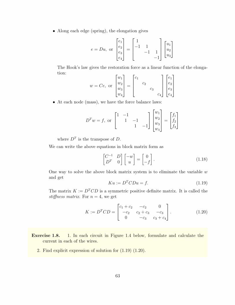
• Along each edge (spring), the elongation gives
e = Du, or
e1
e2
e3
e4
=
1−1 1
−1 1−1
u1
u2
u3
The Hook’s law gives the restoration force as a linear function of the elonga-tion:
w = Ce, or
w1
w2
w3
w4
=
c1
c2
c3
c4
e1
e2
e3
e4
• At each node (mass), we have the force balance laws:
DTw = f, or
1 −11 −1
1 −1
w1
w2
w3
w4
=
f1
f2
f3
where DT is the transpose of D.
We can write the above equations in block matrix form as[C−1 DDT 0
] [−wu
]=
[0−f
]. (1.18)
One way to solve the above block matrix system is to eliminate the variable wand get
Ku := DTCDu = f. (1.19)
The matrix K := DTCD is a symmetric positive definite matrix. It is called thestiffness matrix. For n = 4, we get
K := DTCD =
c1 + c2 −c2 0−c2 c2 + c3 −c3
0 −c3 c3 + c4
. (1.20)
Exercise 1.8. 1. In each circuit in Figure 1.4 below, formulate and calculate thecurrent in each of the wires.
2. Find explicit expression of solution for (1.19) (1.20).
63

3. (Strang pp.130) Find bases for the four fundamental subspaces of
A1 =
1 2 0 30 2 2 20 0 0 00 0 0 4
, A2 =
111
[1 4].
4. Draw the graph whose incidence matrix is
D =
−1 1 0 0−1 0 1 00 1 0 −10 0 −1 1
.
Figure 1.4: In these circuits, each has two nodes and three wires.
64

Chapter 2
Function Spaces
2.1 Abstract Vector Spaces
An abstract vector space is a set V endowed with addition and multiplication operationswhich satisfy the properties mentioned in Chapter 1. Function spaces are typical examplesof abstract vector spaces. Partial differential equations (PDEs) are treated as equations onsuch function spaces. Usually, function spaces are infinite dimensional. In order to solvethese PDEs on computers, approximation theory is introduced, which approximate infinitedimensional function space by finite dimensional vector spaces. The main task there is toconstruct nice bases for efficient approximation. The polynomials, splines, Fourier basis,wavelets, and some special functions such as Legendre functions, Bessel functions, etc, areexamples of such bases for functions defined on various domains with certain symmetry.
2.1.1 Examples of function spaces
We will consider vector spaces either over R or over C. Let us denote an abstract field byF. In this note, it represents either R or C.
1. Function space: Let S be a set. Consider
F(S,F) := f : S → F is a function.
In F(S,F), we define addition and scalar multiplication by
(f + g)(x) := f(x) + g(x), (αf)(x) = αf(x).
Then F(S,F) endowed with these two operations is a vector space over F. WhenS = 1, ..., n, then F(S,R) = Rn, and F(S,C) = Cn.
2. We denote the space F(N,F) by Fω, which is infinite dimensional. Its elements areinfinite sequence
(a1, a2, · · · ).
65

There are important subspaces of Fω common occurred in partial differential equations:for any p ≥ 1,
`p := a ∈ Fω |∞∑i=1
|ai|p <∞.
For p =∞,`∞ := a ∈ Fω|ai is a bounded sequence.
3. DefineC[a, b] := f : [a, b]→ R is continuous.
With function addition and scalar multiplication, C[a, b] forms a vector space. Notethat the set 1, x, x2, · · · is linearly independent (why?). There are infinite may ofthem. Thus, dimC[a, b] =∞. Similarly,
Ck[a, b] = f : [a, b]→ R with f, f ′, ..., f (k) are continuous.
is a vector space.
4. Define
Lp(a, b) = f : (a, b)→ R|ˆ b
a
|f(x)|p dx <∞, p ≥ 1.
It is called the Lp space. Similarly, we define
Wm,p(a, b) = f : (a, b)→ R|ˆ b
a
(|f(x)|p + |f ′(x)|p + · · ·+ |f (m)(x)|p
)dx <∞,m ≥ 0, p ≥ 1,
the Sobolev spaces of order (m, p). These function spaces play important role in non-linear analysis and PDEs.
5. Let Pn = p(x)| p is a polynomial of degree n. With the polynomial addition andscalar multiplication , Pn is a vector space. We will see later that 1, x, x2, ..., xn isindependent. Since Pn is spanned by 1, x, x2, ..., xn, we have dimPn = n+ 1.
2.1.2 Inner product in abstract vector spaces
Let V be an abstract vector space. An inner product structure on V is a mapping 〈·, ·〉 :V × V → R which satisfies
• For every fixed a ∈ V , 〈a, ·〉 is linear. This means that
〈a, α1b1 + α2b2〉 = α1〈a,b1〉+ α2〈a,b2〉;
• 〈·, ·〉 is symmetric. This means that for any a,b ∈ V , we have
〈b, a〉 = 〈a,b〉.
66

• Positivity: for any a ∈ V , we have 〈a, a〉 ≥ 0 and (〈a, a〉 = 0⇒ a = 0).
A vector space V endowed with such inner product structure 〈·, ·〉 is called an inner-productspace.
1. In `2 space, we define the inner product by
〈a,b〉 =∞∑i=1
aibi.
2. In L2[a, b], we define inner product by
〈f, g〉 =
ˆ b
a
f(x)g(x) dx
2.1.3 Basis in function spaces
1. Hat functions In approximation theory, smooth functions are approximated by somespecial functions defined on grids. Here, we introduce piecewise linear functions forapproximating smooth functions defined on [0, 1].
(a) First, we discretize the domain [0, 1] by grid points x0, x1, ..., xn ⊂ [0, 1], wheren is a given positive integer and 0 = x0 < x1 < · · · < xn−1 < xn = 1.
(b) We consider the vector space
V := f : [0, 1]→ R is continuous and linear on each [xj, xj+1] for j = 0, ..., n
Such functions are called piecewise linear functions. Note that V is closed underfunction addition and scalar multiplication. (check?) Thus, V is a vector spaceover R.
(c) For i = 0, ..., n, let us define a function φi which is continuous and piecewise linearon each [xj, xj+1] and φi(xj) = δij, for j = 0, ..., n. You can check that φini=0 isindependent.
(d) Any function f ∈ V can be expressed as
f(x) =n∑i=0
f(xi)φi(x).
That is, any f ∈ V is uniquely determined by its values at the grid points(x0, ..., xn):
f ↔ (f(x0), f(x1), ..., f(xn)).
Thus, φini=0 is a basis for V and dimV = n+ 1.
67

2. Trigonometric functions Let Tn(R) be the space spanned by the set
S = 1, cosx, sinx, cos 2x, sin 2x, ..., cosnx, sinnx
A function of the form
f(x) = a0 +n∑k=1
(ak cos(kx) + bk sin(kx)) , ak, bk ∈ R,
is called a real-valued trigonometric polynomial of degree n. We show that S is inde-pendent.
Proof. (a) Suppose there are real coefficients a0, a1, ..., an, b1, ..., bn such that
a0 +n∑k=1
(ak cos(kx) + bk sin(kx)) = 0. (2.1)
We want to show all these coefficients are zeros.
(b) We multiply (2.1) by cos(`x), ` = 0, ..., n then integrate in x over [0, 2π]. We get
ˆ 2π
0
(a0 +
n∑k=1
(ak cos(kx) + bk sin(kx))
)cos(`x) dx = 0.
We applyˆ 2π
0
cos(kx) cos(`x) dx =
ˆ 2π
0
1
2(cos((k + `)x) + cos((k − `)x)) dx = πδk,`
ˆ 2π
0
sin(kx) cos(`x) dx =
ˆ 2π
0
1
2(sin((k + `)x) + sin((k − `)x)) dx = πδk,`
to geta`π = 0, for ` = 0, ..., n.
(c) Similarly, we multiply (2.1) by sin(`x), ` = 1, ..., n, then integrate in x over [0, 2π],we get
b`π = 0, for ` = 1, ..., n.
We conclude that 1, cosx, sinx, ..., cosnx, sinnx is independent.
3. Chebyshev polynomials. On interval [−1, 1], we consider the function
Tn(x) := cos(nθ), θ = cos−1(x), x ∈ [−1, 1], θ ∈ [0, π]
These functions are called the Chebyshev functions of the first kind. This is anotherkind of special function to approximate functions defined on interval. The function Tnis a polynomial.
68

• n = 0: T0(x) = 1.
• n = 1: T1(x) = cos (cos−1(x)) = x.
• n = 2: T2(x) = cos(2θ) = 2 cos2 θ − 1 = 2x− 1.
• We claim thatTn+1(x) = 2xTn(x)− Tn−1(x). (2.2)
From this and T0 = 1, T1 = x, by mathematical induction, we can get that Tn isa polynomial of degree n. The recursive formula (2.2) is obtained from
cos((n+ 1)θ) = cosnθ cos θ − sinnθ sin θ
cos((n− 1)θ) = cosnθ cos θ + sinnθ sin θ
Adding these two, we get
cos((n+ 1)θ) + cos((n− 1)θ) = 2 cosnθ cos θ
Since cos θ = x, we get (2.2). Note that
ˆ 1
−1
Tn(x)Tm(x)dx√
1− x2=
ˆ π
0
Tn(cos θ)Tm(cos θ)d cos θ√
1− cos2 θ
=
ˆ π
0
cos(nθ) cos(mθ) dθ
=
0 if m 6= nπ if m = n = 0π2
if m = n 6= 0
Thus Tknk=0 constitutes a basis in Pn. They are orthogonal with the innerproduct
〈f, g〉 :=
ˆ 1
−1
f(x)g(x)dx√
1− x2.
69

70

Chapter 3
Linear Transformations
3.1 Linear Transformations–Introduction
1. Let V and W be two vector spaces over a field F. A function T : V → W is called alinear transformation, or a linear map, if T preserves the linear structure. That is
T (αv1 + βv2) = αT (v1) + βT (v2)
for any scalars α, β and any vectors v1,v2 ∈ V .
2. A linear map T : V → W is uniquely determined by its images on the basis. Supposev1, ...,vn is a basis of V . Their images under T are Tv1, ..., Tvn. For any v ∈ V , vcan be represented as v =
∑nj=1 xjvj. Then
Tv = T
(n∑j=1
xjvj
)=
n∑j=1
xjT (vj).
Thus, Tv is uniquely determined by Tv1, ..., Tvn.
3. An m × n matrix A induces a linear map from Rn → Rm by matrix multiplication:x 7→ Ax, where x is represented as an n× 1 column vector, and Ax, the matrix-vectormultiplication, is an m× 1 column vector.
For an abstract linear map T , sometimes, we write T (v) by Tv in order to be consistentto the notation of matrix multiplication.
3.1.1 Linear transformations in R2
1. A linear transformation A : R2 → R2 is uniquely determined by its images on the basise1, e2. Suppose Ae1 = a1 and Ae2 = a2. Then any v = x1e1 + x2e2 is mapped tox1a1 + x2a2. In particular, A0 = 0. We write A = [a1, a2].
71

2. Stretching in R2: Let
A = λI,
Then Ax = λx. We call such mapping a stretching.
3. Rotation in R2: Let
Rθ :=
[cos θ − sin θsin θ cos θ
]Then
Rθe1 =
[cos θsin θ
], Rθe2 =
[− sin θcos θ
]Any vector x ∈ R2 is mapped to
Rθx = R (x1e1 + x2e2) = x1
[cos θsin θ
]+ x2
[− sin θcos θ
]=
[cos θ − sin θsin θ cos θ
] [x1
x2
].
Figure
4. Shearing in R2.
S =
[1 a0 1
]is a shearing operator. It maps[
1 a0 1
] [10
]=
[10
],
[1 a0 1
] [01
]=
[a1
].
This operator appears in continuum mechanics.Figure
5. Orthogonal Projection. Suppose u 6= 0. The projection of any vector v onto thevector u is given by
Pu(v) =1
‖u‖2(u · v)u.
In matrix form, it is
Pu =1
‖u‖2uuT .
Figure
6. Oblique projection. Let u, u ∈ R2. The mapping
Pu,u :=1
uTuuuT
projects a vector v to uTv〈uTu〉u.
72

7. Reflection in R2. Let 0 6= u ∈ R2. A reflection of v ∈ R2 with respect to u is anothervector w ∈ R2 such that (w − v) ⊥ u and v+w
2‖ u. The vector v − Pu(v) ⊥ u. This
gives w = v−2(v−Pu(v)) = (2Pu−I)(v). The matrix representation of the reflectionabout u is
2
‖u‖2uuT − I.
Figure
Remark In the above examples, (1),(3),(5) do not use the orthogonality, whereas (2),(4),(6)use concept of orthogonality.
3.1.2 The space of linear transformations
1. We denote the space of all m-by-n matrices by Mm×n.
Mm×n := A|A is an m× n matrix.
Let us abbreviate Mn×n by Mn. That is,
Mn := A|A is an n× n matrix.
The set Mm×n with matrix addition and scalar multiplication forms a vector space.
2. In Mm×n, let the matrix ek` be defined to be 1 at entry (k, `) and 0 elsewhere. Thenek,`|k = 1, ...,m, ` = 1, ..., n is a natural basis in Mm×n. We thus have
dimMm×n = mn.
In M2×2, the set
e1,1 =
[1 00 0
], e1,2 =
[0 10 0
], e2,1 =
[0 01 0
], e2,2 =
[0 00 1
]constitutes a basis.
3. We denoteL(V,W ) = T : V → W is linear .
Note that L(V,W ) is a vector space as well. In L(V,W ), we define addition andmultiplication by function addition and multiplication. That is, suppose T1, T2 ∈L(V,W ), define T1 + T2 as a map V → W by
(T1 + T2)(v) := T1(v) + T2(v),
If α ∈ R and T ∈ L(V,W ), define
(αT )(v) := αT (v).
You can check that L(V,W ) is closed under the above function addition and scalarmultiplication. Thus, it is a vector space. We abbreviate L(V, V ) by L(V ).
73

4. Suppose v1, ...,vn be a basis of V and w1, ...,wm a basis of W . For k = 1, ..., n and` = 1, ...m, let us define the linear map Tk,` : V → W by
Tk,`(vj) =
w` if j = k0 otherwise,
for j = 1, ..., n.
The definition of Tk,` on the basis v1, ...,vn is extended to all v ∈ V by linearity ofTk,`. Thus, Tk,` ∈ L(V,W ). You can show that Tk,`|k = 1, ..., n, ` = 1, ...,m is a basisof L(V,W ).
Exercise 3.1. 1. What is the matrix J that is a 90 rotation in R2? Show thatJ2 = −I.
2. Suppose P is an orthogonal projection. Show that P 2 = P . Show the same resultwhen P is an oblique projection.
3. On R2, show that the rotation matrix Rθ satisfies Rθ1Rθ2 = Rθ1+θ2 .
4. Find the rotation in R3 that has z-axis as the rotation axis and θ as the rotationangle.
5. (Kazdan) Construct the linear map that maps F to F. Also find its inverse (seefigure).
74

3.2 General Theory for Linear Transformations
The general theory of linear transformation is based on the vector space structure. Noorthogonality concept is involved. Which is replaced by somewhat more general concept, theduality.
3.2.1 Fundamental theorem of linear maps
Let V,W be two vector spaces over a field F. Let T : V → W be a linear map.
1. Kernel and Range We define the kernel of T as
N(T ) := v ∈ V |T (v) = 0,
the range of T asR(T ) := Tv|v ∈ V .
One can check that N(T ) and R(T ) are subspaces of V and W, respectively.
2. Example:
• Hyperplane in Rn: Let α : Rn → R be defined as
α(x) = a1x1 + · · ·+ anxn.
ThenN(α) = x ∈ Rn|a1x1 + · · ·+ anxn = 0
If a := (a1, ..., an) 6= 0, then at least some ai 6= 0. Then
R ⊃ R(α) ⊃ a · x|xi ∈ R, xj = 0 for j 6= i = R.
This shows R(α) = R.
• Hyperplane in V : Let α : V → R be a linear map. The set
N(α) = v|α(v) = 0
is the kernel of α. We will show later that it is a hyperplane in V if α 6= 0. Whichmeans that
dimN(α) = dimV − 1.
In fact, if α 6= 0, then there must be a v ∈ V such that α(v) 6= 0. With this v,we get
Span(α(v)) = R.
Thus,R ⊃ R(α) ⊃ Span(α(v)) = R.
75

• Intersection of hyperplanes: Let αi : V → R, i = 1, 2 be linear maps. Let
T (v) =
[α1(v)α2(v)
]Then
T : V → R2.
The kernel of T is
N(T ) = v ∈ V |αi(v) = 0 = N(α1) ∩N(α2).
is the intersection of two hyperplanes. If R(T ) = 2, that is, two independentconstraints, then dimN(T ) = dimV − 2.
3. Fundamental Theorem of Linear Maps.Many properties of linear maps are derived from dimension arguments. Below is thefundamental one.
Theorem 3.1 (Fundamental Theorem of Linear Maps). Let F be a field and V,Wbe two vector spaces over F. Suppose T : V → W is a linear map. Then
dimN(T ) + dimR(T ) = dimV. (3.1)
Proof. (a) Suppose dimN(T ) = k. k ≥ 0. Let us choose v1, ...,vk as a basis forN(T ). We can extend them to vk+1, ...,vn to form a basis of V .
(b) We claim that Tvk+1, ..., Tvn is independent. Suppose there are ci, i = k +1, ..., n such that
n∑i=k+1
ciTvi = 0.
By linearity of T , we get
T
(n∑
i=k+1
civi
)= 0.
Thus,∑n
i=k+1 civi ∈ N(T ). This means that there are c1, ..., ck such that
n∑i=k+1
civi =k∑i=1
civi.
From vini=1 being a basis of V , we get all ci = 0 for i = 1, ..., n. This shows thatTvi|i = k + 1, ..., n is independent.
76

(c) We claim that R(T ) = Span(Tvk+1, ..., Tvn).
R(T ) = Tv|v ∈ V =
T
(n∑i=1
aivi
)|ai ∈ R
=
n∑
i=k+1
aiT (vi) |ai ∈ R
= Span(Tvk+1, ..., Tvn).
Thus, Tvk+1, ..., Tvn constitutes a basis for R(A). We have dimN(T ) = k anddimR(T ) = n− k. This shows (3.1)
Remarks.
• Although the proof uses basis, the result involves only dimensions, which is inde-pendent of choices of bases.
• Many problems in linear algebra can be solved by comparing dimensions. Animportant lemma isIf U ⊂ V a subspace and dimU = dimV , then U = V .
• Let α : V → R. Suppose α 6= 0. Then dimN(α) = dimV − 1. It means that therange of α gives one constraint to the n parameters x1, ..., xn, resulting in (n− 1)free parameters in the kernel subspace.
4. One-to-one and Onto
• “1-1” means that: if v1 6= v2, then Tv1 6= Tv2;
• “Onto” means that the range of T is the whole space, that is R(T ) = W .
Lemma 3.1. A linear map T : V → W is 1-1 ⇔ N(T ) = 0.
Proof. (⇒) If there is a v ∈ N(T ) and v 6= 0, then Tv = 0 and T0 = 0. We get thatT is not 1-1.(⇐) If Tv1 = Tv2, then T (v1 − v2) = 0. We get (v1 − v2) ∈ N(T ) which is 0 byour assumption. Thus, v1 = v2.
Theorem 3.2. Let V be a finite dimensional vector spaces. A linear map T : V →V is 1-1 ⇔ it is onto. In this case, we say T is non-singular. Otherwise, we sayT is singular.
Proof. (a) (⇒) If T is 1-1, then N(T ) = 0. Hence, dimR(T ) = dimV . ButR(T ) ⊂ V is a subspace. By Proposition 1.4, we get R(T ) = V .
77

(b) (⇐) If R(T ) = V , then dimR(T ) = dimV . From the fundamental theorem oflinear map, we get dimN(T ) = 0. Thus N(T ) = 0.
Corollary 3.1. Suppose S, T ∈ L(V ). Then S T is nonsingular if and only ifboth S and T are nonsingular.
Proof. (a) If both S and T are nonsingular, then both of them are 1-1. This impliesS T is also 1-1:
S T (x) = 0⇒ T (x) = 0. (∵ S is 1-1)
T (x) = 0⇒ x = 0. (∵ T is 1-1).
This shows S T is 1-1. From the previous theorem, S T ∈ L(V ) is 1-1 isequivalent to S T is nonsingular.
(b) Suppose S T ∈ L(V ) is nonsingular. Then R(S T ) = V . Let us denoteR(T ) = W . Then W ⊂ V . Note that
S : W → V
has range S(W ) = S(T (V )) = V . By the fundamental theorem of linear maps,dimS(W ) ≤ dimW . Thus,
dimV ≤ dimW
This together W ⊂ V , we get W = V . That is, T (V ) = V . We also haveS(V ) = S(W ) = V . Thus, both S and T are onto. By the previous theorem,both S and T are non-singular.
Definition 3.1. • A matrix A ∈Mn is called singular if A is not 1-1.
• A matrix A ∈Mn is said to have a right (resp. left) inverse if there exists B ∈Mn
such that AB = I (resp. BA = I).
• A matrix A is said to be invertible if it there exists a B ∈ Mn such that AB =BA = I. We denote such B by A−1.
Corollary 3.2. A square matrix A ∈Mn has right inverse if and only if it has aleft inverse. In this case, A is non-singular.
78

Proof. (a) Suppose A has a left inverse, call it B. This means that B ∈ Mn andBA = I. By the previous corollary, BA = I implies both B and A are 1-1 andonto. Now, for any y ∈ V , there exists a unique x ∈ V such that Ax = y (becauseA is 1-1 and onto). We have
ABy = AB(Ax) = A(BA)x = AIx = Ax = y.
Thus, AB = I. B is also a right-inverse of A.
(b) Suppose A has right-inverse, called C. This means that C ∈ Mn and AC = I.By the previous corollary, both C and A are 1-1 and onto. For any x ∈ V , thereexists a unique z ∈ V such that Cz = x (because C is 1-1 and onto). We have
CAx = CA(Cz) = C(AC)z = Cz = x.
Thus, CA = I. C is also a left-inverse of A.
5. Isomorphism A linear map T : V → W is called an isomorphism if it is also 1-1 andonto. In this case, we denote its inverse map by T−1, which is also linear.
Let V and W be two vector spaces. If there exists an isomorphism T : V → W , wesay that V is isomorphic to W .
Theorem 3.3. Every n-dimensional vector space over R is isomorphic to Rn.
Proof. We choose a basis B = v1, ...,vn of V . Then every v ∈ V can be representeduniquely by
v =n∑i=1
civi
The mapping T : V → Rn byTv = (c1, ..., cn)
is well-defined. It is 1-1 and onto from the definition of basis.
We denote
[v]B =
c1...cn
and call it as the representation of v under the basis B. Thus, v is expressed as
v =[v1 · · · vn
] c1...cn
=[v1 · · · vn
][v]B.
Corollary 3.3. The space Mm×n is isomorphic to Rmn.
79

Remark The above results hold with R replaced by a general field F.
Exercise 3.2. 1. (a). Suppose T : V → W is 1-1. Show that dimW ≥ dimV .(b). Suppose T : V → W is onto. Show that dimW ≤ dimV .
2. In M2×2, show that the 4 matrices
e1 =
[1 00 1
], e2 =
[0 −11 0
], e3 =
[0 11 0
], e4 =
[1 00 −1
],
constitutes a basis for M2×2.
3. Show that
I =
[1 00 1
], J =
[0 −11 0
]is independent in M2×2. Show that the space spanned by I, J is isomorphic toC.
4. (Axler, pp.67) Give an example of a linear map T : R4 → R4 such that
R(T ) = N(T )
5. (Axler, pp.67)Prove that there does not exist a linear map T : R5 → R5 such that
R(T ) = N(T ).
6. (Axler pp.68) Suppose U, V,W are finite dimensional vector spaces and
US−→ V
T−→ W
be linear maps. Prove that
dimN(T S) ≤ dimN(S) + dimN(T ).
dimR(T S) ≤ mindimR(S), dimR(T ).
3.2.2 Matrix representation for linear maps
1. Coordinate representation for vectors Let V be a vector space. If we choose abasis B = v1, ...,vn, then every vector v ∈ V can be represented as
v =[v1 · · · vn
] c1...cn
=[v1 · · · vn
][v]B.
80

The column vector [v]B is called the coordinate representation of v under B.
2. Matrix representation for linear maps Let T ∈ L(V,W ). Let us choose bases
B1 = v1, ...,vn for V and B2 = w1, ...,wm for W .
Suppose
Tvj =m∑i=1
aijwi, j = 1, ..., n,
we call the matrix A = (aij)m×n the matrix representation of T under the bases B1
and B2. We denote it by[T ]B1,B2 = A.
The matrix representation of T under B1,B2 is expressed as[Tv1 · · · Tvn
]=[w1 · · · wm
][T ]B1,B2 (3.2)
For v ∈ V and the corresponding Tv ∈ W , they can be represented as
v =n∑j=1
xjvj, Tv =m∑i=1
yiwi.
Then
Tv =n∑j=1
xjTvj =n∑j=1
xj
m∑i=1
aijwi =m∑i=1
(n∑j=1
aijxj
)wi =
m∑i=1
yiwi.
Or[Tv]B2 = [T ]B1,B2 [v]B1 (3.3)
Example 1 Let T : V → W . dimV = 3, dimW = 2. Let us choose the standardbasis in both spaces. If
Te1 = 2e1 − e2, Te2 = e1 + 3e2, Te3 = −e1 + 2e2.
That is,
[Te1, Te2, Te3] = [e1, e2]
[2 1 −1−1 3 2
]The matrix representation of T under the standard bases is
[T ]Bs,Bs =
[2 1 −1−1 3 2
].
Suppose we choose B2 = w1,w2:
w1 =
[11
], w2 =
[01
].
81

Then2e1 − e2 = xw1 + yw2
This is [1 01 1
] [xy
]=
[2−1
].
It gives [xy
]=
[1 0−1 1
] [2−1
]=
[2−3
].
Hence, 2e1 − e2 = 2w1 − 3w2. Similarly, we have
e1 + 3e2 = w1 + 2w2, −e1 + 2e2 = −w1 + 3w2.
Thus,Te1 = 2w1 − 3w2, Te2 = w1 + 2w2, Te3 = −w1 + 3w2.
The matrix representation of T under Bs and B is
TBs,B =
[2 1 −1−3 2 3
].
Proposition 3.1. Suppose U, V,W are finite dimensional vector spaces and
US−→ V
T−→ W
be linear maps. Let B1,B2,B3 are bases of U, V,W , respectively. Then we have
[T S]B1,B3 = [T ]B2,B3 [S]B1,B2 . (3.4)
Proof. Suppose B1 = u1, ...,un, B2 = v1, ...,vm and B3 = w1, ...,wp. Supposethe matrix representations of S and T are
Suj =m∑k=1
skjvk, [S]B1,B2 = (skj)m×n
Tvk =
p∑i=1
tikwi, [T ]B2,B3 = (tik)p×m
Then
(T S)uj = T (Suj) = T
(m∑k=1
skjvk
)=
m∑k=1
skjTvk
=m∑k=1
skj
(p∑i=1
tikwi
)=
p∑i=1
(m∑k=1
tikskj
)wi
Thus, the matrix representation of T S under B1 and B3 is the matrix∑m
k=1 tikskj,which is [T ]B2,B3 [S]B1,B2 .
82

Proposition 3.2. Let V be an n-dimensional vector space and W be an m-dimensionalvector space. Then the vector space L(V,W ) is isomorphic to Mm×n.
Proof. We choose a basis B1 = v1, ...,vn for V and a basis B2 = w1, ...,wm for W .Then the mapping
M(T ) := [T ]B1,B2
is a mapping L(V,W )→Mm×n. We show that M is linear, 1-1 and onto.
(a) Linear: Suppose T 1, T 2 are two linear maps in L(V,W ) with [T `]B1,B2 = (t1ij),` = 1, 2. This means that
T `vj =m∑i=1
t`ijwi.
Suppose a, b ∈ R, we have
(aT 1 + bT 2)vj = aT 1vj + bT 2vj =m∑i=1
at1ijwi +m∑i=1
bt2ijwi
=m∑i=1
(at1ij + bt2ij
)wi
This shows
[aT 1 + bT 2]B1,B2 = a[T 1]B1,B2 + b[T 2]B1,B2 .
Thus, the mapping M is linear.
(b) 1-1: If [T ]B1,B2 = 0, we want to show T ≡ 0. [T ]B1,B2 = 0 means that
Tvj =m∑i=1
0wi = 0. for all j = 1, ..., n.
Thus, T ≡ 0.
(c) Onto. Given any matrix A = (aij)m×n. We define
Tvj =m∑i=1
aijwi, j = 1, ..., n.
This defines a linear map T ∈ L(V,W ) with [T ]B1,B2 = A.
83

3. Matrix representation for operators Let T ∈ L(V, V ). We abbreviate L(V, V ) byL(V ). Suppose B = v1, ...,vn is a basis of V . The matrix representation of T is[
Tv1 · · · Tvn]
=[v1 · · · vn
][T ]B (3.5)
Here, we abbreviate [T ]B,B by [T ]B. In terms of coordinate, we have
[Tv]B = [T ]B[v]B. (3.6)
In R3, let us choose the standard basis Bs = e1, e2, e3. Suppose
Te1 = e1 + 2e2 + 3e3,
Te2 = 4e1 + 5e2 + 6e3,
Te3 = 7e1 + 8e2 + 9e3,
the matrix representation of T under Bs is
[T ]Bs =
1 4 72 5 83 6 9
Suppose a vector v = e1 + e3. The coordinate of v is
[v]B =
101
.The transformation Tv is
T (e1 + e3) = Te1 + Te3
= (e1 + 2e2 + 3e3) + (7e1 + 8e2 + 9e3)
= 8e1 + 10e2 + 12e3.
In terms of matrix representation and coordinate, it is
[Tv]B = [T ]B[v]B =
1 4 72 5 83 6 9
101
=
81012
3.2.3 Change-basis formula
1. Basis change formula for vectors Let V be a vector space and suppose B =v1, ...,vn and B′ = v′1, ...,v′n are two bases of V . Let Id : V → V denote theidentity map (i.e. Id(v) = v). The matrix representation of Id under B,B′ is (3.2):[
v1 · · · vn]
=[v′1 · · · v′n
][Id]B,B′ .
84

Then the change-basis formula for vectors is given by (3.3):
[v]B′ = [Id]B,B′ [v]B.
Note that[v]B = [Id]B′,B[v]B′ = [Id]B′,B[Id]B,B′ [v]B
Thus,[Id]B′,B = [Id]−1
B,B′ .
Example 1 (continue) In Example 1, we have two bases in W : the standard basesBs = e1, e2 and B = w1,w2. The matrix representation of the basis-changeformula is
w1 = e1 + e2, w2 = e2,
or equivalently,
[w1,w2] = [e1, e2][Id]B,Bs = [e1, e2]
[1 01 1
].
Recall the matrix representation for T : V → W under standard bases is
[T ]Bs,Bs =
[2 1 −1−1 3 2
].
With the basis Bs in W replaced by B, the matrix representation of T is
[T ]Bs,B = [Id]Bs,B[T ]Bs,Bs = [Id]−1B,Bs [T ]Bs,Bs
=
[1 0−1 1
] [2 1 −1−1 3 2
]=
[2 1 −1−3 2 3
].
Example 2. In R3, let B = w1,w2,w3, where
w1 =
123
, w2 =
456
, w3 =
789
.Then
[Id]B,Bs =
1 4 72 5 83 6 9
2. Basis change formula for operators. Suppose T ∈ L(V ). Suppose B and B′ are
two bases of V . We have
[Tv]B = [T ]B[v]B, [Tv]B′ = [T ]B′ [v]B′
85

[v]B′ = [Id]B,B′ [v]B, [Tv]B = [Id]B′,B[Tv]B′
Thus, we obtain[T ]B′ = [Id]B,B′ [T ]B[Id]B′,B.
Note that from Proposition 3.1,
[Id]B,B′ [Id]B′,B = I.
We have[T ]B′ = S[T ]BS
−1, where S = [Id]B,B′ . (3.7)
Example 3 Suppose T : R3 → R3 has the representation under standard basis Bs =e1, e2, e3:
[T ]Bs =
2 1 30 1 21 0 1
Consider another basis B = w1,w2,w3,
w1 =
100
, w2 =
110
, w3 =
011
.Then
[Id]B,Ss = [w1,w2,w3] =
1 1 00 1 10 0 1
.The matrix representation of T under B is
[T ]B = [Id]Bs,B[T ]Bs [Id]B,Bs
=
1 1 00 1 10 0 1
−1 2 1 30 1 21 0 1
1 1 00 1 10 0 1
=
1 −1 10 1 −10 0 1
2 1 30 1 21 0 1
1 1 00 1 10 0 1
=
3 3 2−1 0 21 1 1
.3. Similarity of matrices. Two matrices A and B are called similar if there is an
invertible matrix S such that A = SBS−1. Thus, the matrices that representing anoperator are all similar. Conversely, the class of all similar matrices corresponds to anoperator.
86

Exercise 3.3. 1. (Schaum’s pp. 299) Let
A =
[2 5 −31 −4 7
]be the matrix representation of a linear map T : R3 → R2 under the standardbases. Now, we choose B1 = v1,v2,v3 and B2 = w1,w2. Find the matrixrepresentation [T ]B1,B2 .
v1 =
111
, v2 =
110
, v3 =
100
, w1 =
[13
], w2 =
[25
].
2. (Schaum pp. 310) Find the chang-of-basis matrix formula under the above basisv1,v2,v3 in the previous problem for the matrix1 3 2
1 0 −40 1 3
.3. Represent
v =
[13
]In terms of
v1 =
[1−1
], v2 =
[21
]and in terms of
v′1 =
[1−1
], v′2 =
[1
−1 + 0.001
]4. Let T ∈ L(R2). Let
[T ]Bs =
[3 1−1 2
],
where Bs stands for the standard basis e1, e2. Find the representation of T under
B1 = v1,v2, v1 =
[1−1
], v2 =
[21
],
87

and under
B′1 = v′1,v′2, v′1 =
[1−1
], v′2 =
[1
−1 + 0.001
].
Find the similarity transform matrix S = [Id]B,B′ .
5. Find the coordinates of (a, b, c) with respective to the basis B = v1,v2,v3,
v1 =
120
, v2 =
132
, v3 =
013
.This means that we want to find the coordinates (x, y, z) such thatab
c
= x
120
+ y
132
+ z
013
.6. Prove Proposition 3.1.
7. Complete the proof of Proposition 3.2.
3.3 Duality
3.3.1 Motivations
Duality is a very fundamental concept in linear algebra. It is a pair of two quantities a,b withthe same number of components, but different physical meaning. They are arisen naturallyfrom applications. Thus, let us learn this concept from some concrete examples.
Examples in finite dimensions
1. Suppose we have n commodities, say, item 1 to item n. There are two quantitiesassociated with each item: the price ai and the amount bi. Let a = (a1, ..., an),b = (b1, ..., bn). We may call the space spanned by a the price space, the spacespanned by b the quantity space. Although both spaces are isomorphic to Rn, theyare different in application sense. Yet, they are paired to each other, or dual to eachother from application point of view. If we denote the price space by V , we will denotethe quantity space by V ∗, the dual space of V .
2. Let us consider the spring-mass system in a graph G = (V,E). At each node j, we canassociate it with mj, the displacement uj, the force fj = mjg. We say (uj, fj) are dualto each other because in application, we use
∑j fjuj for the work done by the system.
Similarly, on the edges, we can associate elongation (strain) ei and restoration force
88

(stress) wi. There is also a connection between them. Namely∑
i eiwi is the potentialenergy of the system.
3. Let V = v1, ..., vn be a set of vertices. We define a formal vertex space to be
V := n∑j=1
ajvj| aj ∈ R.
This space is dual to F(V,R). A function f ∈ F(V,R) is paired with an elementa =
∑nj=1 ajvj by
〈f , a〉 =∑j
ajf(vj) =∑j
ajfj.
In above examples, the pairing of a and b (or f) comes from applications. If the spaceformed by all possible a is V . We denote The space formed by all possible dual variableby V ∗. Although both of them is isomorphic to Rn, (or Fn if the underlying field is F) wedistinguish them from the nature of applications.
Examples in infinite dimensions Duality also appears naturally in infinite dimensionalfunction spaces. Consider V = C[0, 1], the set of all continuous functions on [01, ]. Let useconsider the following maps for f ∈ C[0, 1]:
• f 7→´ 1
0f(x) dx;
• f 7→ f(x1), where x1 ∈ [0, 1] is a fixed point;
• Given xi ∈ [0, 1] and ai, I = 1, ..., n, the map is defined as
f 7→n∑i=1
aif(xi).
In these examples, the pairing object with the function f is a geometric object. In the firstexample, it is the interval [0, 1]. In the second example, it is a fixed point x1 ∈ [0, 1]. Inthe third example, it is a set of points x1, ..., xn together with weights a1, ..., an. All of thesegeometric objects lie in the dual space of C[0, 1]. In real analysis, you will learn that thedual space of C[0, 1] is the set of all measurable sets on [0, 1].
3.3.2 Dual spaces
The concept of duality will replace the inner product structure in our earlier study. Thus,the fundamental theorem of linear algebra can be build only on the vector space structure,no need on the inner-product structure. First, the normal a is replaced by a linear functionalα; and the hyperplane U defined by a · x = 0 is replaced by the annihilator of the linearfunctional α.
89

1. Linear functionals and Dual Spaces
(a) A linear function α : V → F is called a linear functional on V .
(b) Let us choose a basis B = v1, ...,vn for V . Then, given a linear functionalα : V → F, it has the representation
α(x) = a1x1 + · · ·+ anxn,
where
x =n∑i=1
xivi, ai = α(vi).
Conversely, given (a1, ..., an) ∈ Fn, it induces a linear functional α : V → F suchthat
α(vi) = ai, I = 1, ..., n.
Thus, with the help of a basis B, a linear functional α is equivalent to a rowvector (a1, ..., an).
(c) The set of all linear functionals on V is a vector space, and is called the dual spaceof V . We denote it by V ∗. That is, V ∗ = L(V,F). An element α ∈ V ∗ is alsocalled a covector. From Corollary 3.3, V ∗ is isomorphic to M1×n, the space ofrow vectors of size n.
(d) In the example of commodity price, let a = (a1, ..., an) be the price, (x1, ..., xn)the quantity of the commodity. Let us denote the space formed by all possible xby V . On V , given a price list a, we define the price functional as
α(x) := a1x1 + · · ·+ anxn.
The function α is a linear functional on V . There is a natural correspondencebetween the price list a := (a1, ..., an) and the price functional α. We can use α toreplace a, because the price for each commodity can be obtained from ai = α(vi).
(e) Recall that, the formulaa1x1 + · · ·+ anxn,
which was interpreted as the inner product of a and x, is not natural from ap-plication of view, because a and x are not in the same space. Here, it is morenatural to interpret it as the representation of a linear functional α under somebasis B in V .
2. Geometric picture of a linear functional Following the above discussion, we shallgive a geometric picture in V for a covector α, which does not involve an inner productstructure. We claim that a geometric picture of a covector α can be interpreted by thefollowing affine hyperplane:
Sα := x ∈ V |α(x) = 1. (3.8)
Conversely, given an affine hyperplane S, we can construct a linear functional α suchthat S = Sα. Let us explain this below.
90
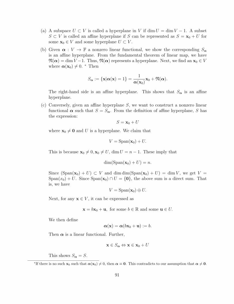
(a) A subspace U ⊂ V is called a hyperplane in V if dimU = dimV − 1. A subsetS ⊂ V is called an affine hyperplane if S can be represented as S = x0 + U forsome x0 ∈ V and some hyperplane U ⊂ V .
(b) Given α : V → F a nonzero linear functional, we show the corresponding Sα
is an affine hyperplane. From the fundamental theorem of linear map, we haveN(α) = dimV −1. Thus, N(α) represents a hyperplane. Next, we find an x0 ∈ Vwhere α(x0) 6= 0. ∗ Then
Sα := x|α(x) = 1 =1
α(x0)x0 + N(α).
The right-hand side is an affine hyperplane. This shows that Sα is an affinehyperplane.
(c) Conversely, given an affine hyperplane S, we want to construct a nonzero linearfunctional α such that S = Sα. From the definition of affine hyperplane, S hasthe expression:
S = x0 + U
where x0 6= 0 and U is a hyperplane. We claim that
V = Span(x0) + U.
This is because x0 6= 0,x0 6= U , dimU = n− 1. These imply that
dim(Span(x0) + U) = n.
Since (Span(x0) + U) ⊂ V and dim dim(Span(x0) + U) = dimV , we get V =Span(x0) + U . Since Span(x0) ∩ U = 0, the above sum is a direct sum. Thatis, we have
V = Span(x0)⊕ U.
Next, for any x ∈ V , it can be expressed as
x = bx0 + u, for some b ∈ R and some u ∈ U.
We then define
α(x) = α(bx0 + u) := b.
Then α is a linear functional. Further,
x ∈ Sα ⇔ x ∈ x0 + U
This shows Sα = S.
∗If there is no such x0 such that α(x0) 6= 0, then α ≡ 0. This contradicts to our assumption that α 6= 0.
91

3. Dual basis Suppose B = v1, ...,vn is a basis of V . Recall that a linear transfor-mation is uniquely determined by its values on a basis. We thus define the linearfunctionals v∗i , i = 1, ..., n by
v∗i (vj) = δij, j = 1, ..., n.
Then B∗ := v∗1, ...,v∗n is a basis for V ∗. It is called the dual basis of B. AS aconsequence,
dimV ∗ = dimV.
Proof.
(a) Independence: suppose there are coefficients c1, ..., cn such that
c1v∗1 + · · ·+ cnv
∗n = 0.
Then (n∑i=1
civ∗i
)(vj) = 0 for all j = 1, ..., n.
But the left-hand side isn∑i=1
civ∗i (vj) =
n∑i=1
ciδij = cj.
We get all cj = 0. Thus, v∗1, ...,v∗n is independent.
(b) Span: V ∗ = Span(v∗1, ...,v∗n. For any α ∈ V ∗, we claim that
α =n∑j=1
ajv∗j , with aj = α(vj).
For any v ∈ V , it can be expressed under B by
v =n∑i=1
xivi.
Then
α(v) = α
(n∑i=1
xivi
)=
n∑i=1
xiα(vi)
On the other hand,(n∑j=1
α(vj)v∗j
)(v) =
n∑j=1
α(vj)v∗j
(n∑i=1
xivi
)=
n∑j=1
α(vj)n∑i=1
xiδij =n∑i=1
xiα(vi)
Thus,
α =n∑j=1
α(vj)v∗j .
92

4. Representation of vectors and covectors
We have the following representation of v ∈ V and α ∈ V ∗ under the bases B and B∗:
[v]B =
v∗1(v)...
v∗n(v)
, [α]B∗ =
α(v1)...
α(vn)
.Note that α also has a matrix representation. With the basis B for V and the unity1 the basis for F, the matrix representation of the linear functional α : V → F is
[α]B,1 = [α(v1), ...,α(vn)] = [α]TB∗ .
With these representations, we can write
α(v) = α
(n∑i=1
xivi
)=
n∑i=1
aixi = [α]TB∗ [v]B = [α]B,1[v]B.
where
[α]B,1 = [a1, ..., an], [v]B =
x1...xn
.5. Double dual.
Lemma 3.2. . Let V be a finite dimensional vector space. We have
(V ∗)∗ = V.
Here, (V ∗)∗ is the dual of V ∗. We denote it by V ∗∗.
(a) V ⊂ V ∗∗. Any v ∈ V can be thought as a linear functional on V ∗ by
α 7→ α(v).
By function addition and scalar multiplication, we have
(α + β)(v) = α(v) + β(v)
(aα)(v) = aα(v).
Thus, v ∈ V ∗∗.(b) We recall Lemma 1.4: If U ⊂ V is a subspace and dimU = dimV , then U = V .
Here, we havedimV = dimV ∗ = dimV ∗∗.
By Lemma 1.4, we have V = V ∗∗
93
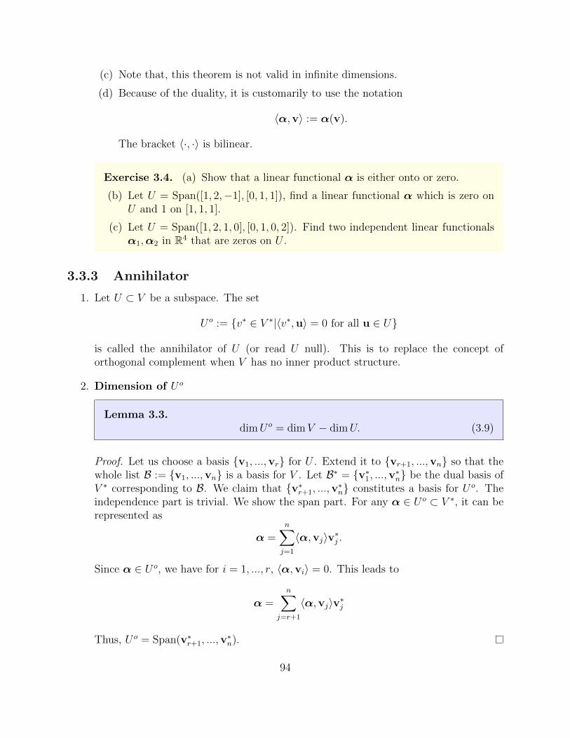
(c) Note that, this theorem is not valid in infinite dimensions.
(d) Because of the duality, it is customarily to use the notation
〈α,v〉 := α(v).
The bracket 〈·, ·〉 is bilinear.
Exercise 3.4. (a) Show that a linear functional α is either onto or zero.
(b) Let U = Span([1, 2,−1], [0, 1, 1]), find a linear functional α which is zero onU and 1 on [1, 1, 1].
(c) Let U = Span([1, 2, 1, 0], [0, 1, 0, 2]). Find two independent linear functionalsα1,α2 in R4 that are zeros on U .
3.3.3 Annihilator
1. Let U ⊂ V be a subspace. The set
U o := v∗ ∈ V ∗|〈v∗,u〉 = 0 for all u ∈ U
is called the annihilator of U (or read U null). This is to replace the concept oforthogonal complement when V has no inner product structure.
2. Dimension of U o
Lemma 3.3.dimU o = dimV − dimU. (3.9)
Proof. Let us choose a basis v1, ...,vr for U . Extend it to vr+1, ...,vn so that thewhole list B := v1, ...,vn is a basis for V . Let B∗ = v∗1, ...,v∗n be the dual basis ofV ∗ corresponding to B. We claim that v∗r+1, ...,v
∗n constitutes a basis for U o. The
independence part is trivial. We show the span part. For any α ∈ U o ⊂ V ∗, it can berepresented as
α =n∑j=1
〈α,vj〉v∗j .
Since α ∈ U o, we have for i = 1, ..., r, 〈α,vi〉 = 0. This leads to
α =n∑
j=r+1
〈α,vj〉v∗j
Thus, U o = Span(v∗r+1, ...,v∗n).
94

3. The double annihilator. We have identify (V ∗)∗ = V . The annihilator of a subsetU ⊂ V ∗ is defined to be
U o := v ∈ V |〈u,v〉 = 0 for all u ∈ U.
Lemma 3.4. Let U ⊂ V be a subspace. Then the double annihilator of U is itself.
(U o)o = U.
Proof. (a) We show U ⊂ U oo. For any u ∈ U any u∗ ∈ U o, we have
〈u∗,u〉 = 0
This also means u annihilates U o. Thus, u ∈ (U o)o.
(b) From Lemma 3.3, we get
dimU oo = dimV ∗ − dimU o = dimV − (dimV − dimU) = dimU.
Thus, U ⊂ U oo and have same dimensions, we get U = uoo.
Exercise 3.5. (a) Suppose U1 ⊂ U2 ⊂ V are two subspace. Show that U o2 ⊂ U o
1 .
(b) Suppose U1, U2 ⊂ V are two subspaces. Show that
(U1 + U2)o = U o1 ∩ U o
2 .
(c) Suppose α1, ...,αr is independent in V ∗. Let U = v|α1(v) = 0, ...,αr(v) =0. Show that dimU = dimV − r.
3.3.4 Dual maps
1. Let V,W be vector spaces over F with dimensions n and m, respectively. Let
T : V → W
be a linear map. The map T induces a linear map
T ∗ : W ∗ → V ∗ by T ∗β := β T for any β ∈ W ∗.
This definition is equivalent to say that for any β ∈ V ∗ and for any v ∈ V , T ∗ satisfies
T ∗β(v) = β(Tv).
In terms of the notation 〈α,v〉 := α(v), it is
〈T ∗β,v〉 := 〈β, Tv〉.
95

2. Representation of T ∗
Proposition 3.3. Suppose B1 = v1, ...,vn is a basis of V , B2 = w1, ...,wm abasis of W . Their duals B∗1 = v∗1, ...,v∗n and w∗1, ...,w∗m are respectively basesof V ∗ and W ∗. We have
[T ∗]B∗2 ,B∗1 = [T ]TB1,B2 .
Here, the right-hand side is the transpose of the complex-valued matrix [T ]B1,B2 .
Proof. We have〈w, Tv〉 = [w]TB2 [Tv]B2 = [w]TB2 [T ]B1,B2 [v]B1 .
〈T ∗w∗,v〉 = [T ∗w∗]TB∗1 [v]B1 =([T ∗]B∗2 ,B∗1 [w∗]B2
)T[v]B1
From 〈w∗, Tv〉 = 〈T ∗w∗,v〉 for all v and f¯w∗, we get
[T ∗]TB∗2 ,B∗1 = [T ]B1,B2 .
3. Double dual is itself.
Lemma 3.5.T ∗∗ = T.
Proof. The mapping T ∗∗ : V ∗∗ → W ∗∗. Since V = V ∗∗ and W = W ∗∗. For any v ∈ Vand any w∗ ∈ W ∗, we have
〈T ∗∗v,w∗〉 = 〈v, T ∗w∗〉 = 〈Tv,w∗〉
4. The dual of composition.
Lemma 3.6. If T, S ∈ L(V ), then (T S)∗ = S∗ T ∗.
Proof. For any v ∈ V and any w∗ ∈ V ∗, we have
〈(T S)v,w∗〉 = 〈T (Sv),w∗〉 = 〈Sv, T ∗w∗〉 = 〈v, S∗(T ∗w∗)〉 = 〈v, (S∗ T ∗)w∗〉
On the other hand,〈(T S)v,w∗〉 = 〈v, (T S)∗w∗〉.
Thus, 〈v, (T S)∗w∗〉 =< v, (S∗ T ∗)w∗〉 for any v ∈ V and any w∗ ∈ V ∗. We get(T S)∗ = S∗ T ∗.
96

Exercise 3.6. 1. Let I : V → V be the identity map. Show that I∗ is also theidentity map in V ∗.
3.4 Fundamental Theorem of Linear Algebra
Theorem 3.4 (Fundamental theorem of linear algebra). Let V and W be vector spacesover F with dimensions n and m. Let
T : V → W
be a linear map. Then
(a) N(T ) = R(T ∗)o, N(T ∗) = R(T )o
(b) dimR(T ∗) = dimR(T )
(c) R(T ∗) = N(T )o, R(T ) = N(T ∗)o
Proof. 1. We show (a).
v ∈ R(T ∗)o ⇔ 〈T ∗β,v〉 = 0 for all β ∈ W ∗
⇔ 〈β, Tv〉 = 0 for all β ∈ W ∗
⇔ Tv = 0⇔ v ∈ N(T ).
2. To show N(T ∗) = R(T )o, we use duality argument. We apply the previous statementto T ∗ to get
N(T ∗) = R(T ∗∗)o = R(T )o.
3. We show (b).
dimR(T ∗) = dimW − dimN(T ∗)
= dimW − dimR(T )o
= dimR(T )
The first equality is from the fundamental theorem of linear map for T ∗; the second isfrom (a); the third one is from Lemma 3.3.
4. To show (c), we take annihilation of the equalities in (a) to get
N(T )o = R(T ∗)oo = R(T ∗)
AndN(T ∗)o = R(T )oo = R(T ).
Here, Lemma 3.4 is used.
97

Remark The four fundamental subspace theorem in the case of inner product, it is harderto show
N(T )⊥ = R(T ∗)
Or equivalently, it is the same problem to show U⊥⊥ = U , see Corollary 1.1 . What is behindis the Riesz representation theorem when we want to show U⊥⊥ = U . We will study this inthe next Chapter. In our present case, U oo = U is much easier.
Exercise 3.7. 1. Consider
D =
1 −1 0 00 1 −1 00 0 1 −1
It is a linear map from R4 to R3. Find N(D), N(DT ).
2. Prove Corollary 3.1.
3. Prove Corollary 3.2.
3.5 Applications
3.5.1 Topological property of the graphs
Let us study topological property of the graphs. Let G = (V,E) be a directed graph.
1. The connectivity of a graph is encoded by the incident matrix D = (dij)m×n definedby
dij =
−1 if edge i starts at vertex j1 if edge i ends at vertex j0 otherwise
For each row (i.e. edge), there is a −1 (starting node) and a +1 (end node). The totalsum of each row is 0.
In the above Example 1, The vertices V = 1, 2, 3, 4 and edges
E = (4, 1), (1, 2), (1, 3), (2, 3), (2, 4), (3, 4).
Let label the edges in order from edge 1 to edge 6. The corresponding incident matrixis
D =
1 0 0 −1−1 1 0 0−1 0 1 00 −1 1 00 −1 0 10 0 −1 1
edges×vertices
98

2. Suppose G = (V,E) is a directed graph. Our goal is to understand the meaning of thefour subspaces associated with the corresponding incident matrix D. There are fourvector spaces naturally associated with G:
• Vertex space: C0(G) := R|V |,• Edge space: C1(G) := R|E|,• Dual vertex space Ω0(G) := x : V → R This space is still the same as R|V |,• Dual edge space Ω1(G) := y : E → R. It is the same as R|E|.
Here, |V | denotes for the number of vertices in V . Suppose |V | = n and |E| = m.
(a) Vertex space. C0(G) is spanned by ej, j = 1, ..., n. ej represents vertex j. Anelement c0 ∈ C0(G) is represented as c0 =
∑nj=1 ajej.
(b) Edge space. The linear combination of edges with integer coefficients can bethought as a path of the graph. For instance, (1, 2) + (2, 4)− (3, 4) is a path goingthrough the edges (1, 2), (2, 4), (4, 3). In terms of the labeled edges (i.e. (1, 2)is labeled as edge 2 and represented as e2 in edge space C1(G), (2, 4) is labeledby 5 (e5 ∈ C1(G)) and (3, 4) by 6 (e6 ∈ C1(G)), a path is a vector in the edgespace with integer coefficients. In this example, c = [0, 1, 0, 0, 1,−1]T ∈ C1(G)represents the path: edge 2 + edge 5 - edge 6.
(c) Dual vertex space Ω0(G). An element x ∈ Ω0(G) is merely a function definedon vertices. For instance, x = (x1, ..., xn) is the electric potential in an electricalgraph. There is a natural pairing between an element x ∈ Ω0(G) and an elementc0 =
∑nj=1 ajej ∈ C0(G) by
〈x, c0〉 :=n∑j=1
xjaj.
For instance, if c0 = [1, 0, 0,−1]T , then 〈x, c0〉 measures the potential differencex1 − x4. From the bilinear structure of 〈·, ·〉, we say that Ω0(G) is the dual spaceof C0(G).
(d) Dual edge space Ω1(G). Similarly, an element y ∈ Ω1(G) is a function definedon edges. For instance, y = (y1, ..., ym) represents the electric current in an electricgraph. There is also a natural pairing between an element c1 =
∑mi=1 biei ∈ C1(G)
and an element y ∈ Ω1(G), defined by
〈y, c1〉 :=m∑i=1
yibi.
In example 1, if c1 = e1 − e2 − e3 (that is, (4, 1)− (1, 2)− (1, 3)), then
〈y, c1〉 = y1 − y2 − y3,
which is the total current flowing into node 1.
99

3. Incident matrix D can be thought as a linear map
D : Ω0(G)→ Ω1(G).
Suppose x ∈ Ω0(G). Then Dx ∈ Ω1(G), a function defined on edges. Suppose e =(j1, j2), then
Dx(e) = xj2 − xj1 .
Thus, D is a difference operator.
4. DT is a boundary operator. DT , the dual of D, is thought as: DT : C1(G)→ C0(G)satisfying: for any c1 ∈ C1(G),
〈x, DTc1〉 = 〈Dx, c1〉 for any x ∈ Ω0(G).
Given an edge, say edge 2, or equivalently, z = [0, 1, 0, 0, 0, 0]T ∈ C1(G).
DTz =
1 −1 −1 0 0 00 1 0 −1 −1 00 0 1 1 0 −1−1 0 0 0 1 1
010000
=
−1100
.
Thus, DTz gives the signed values of the boundary of z. (Starting node has value −1,end node has value 1.) In our early example where c = [0, 1, 0, 0, 1,−1]T , the pathstarts from node 1 and ends at node 3. The corresponding DTc is −1 at the startingnode, and −1 at the ending node. That is,
1 −1 −1 0 0 00 1 0 −1 −1 00 0 1 1 0 −1−1 0 0 0 1 1
01001−1
=
−1010
.
Thus, DT transforms a path to its boundary: with 1 at the ending node and −1 at thestarting node, and 0 at the rest nodes. We call DT the boundary operator.
5. What is N(DT )? A closed path is a path with ending node equals the starting node.It is also called a loop. Thus, a loop c is a vector in the edge space such that DTc = 0.Thus,
N(DT ) = Span of loops in C1(G).
100

We look for a basis for N(DT ). In example 1, N(DT ) has a basis c1, c2, c3, where
c1 :=
101001
, c2 :=
01−1100
, c3 :=
110010
They correspond to the following loops:
• c1 connecting the nodes (4, 1, 3),
• c2 connecting the nodes (1, 2, 3),
• c3 connecting (4, 1, 2).
6. In example 2 of the last subsection, V = 1, 2, 3, 4, 5, E = (1, 2), (2, 3), (3, 1), (4, 5).This graph consists of two components. The vertices 1, 2, 3 is in one component con-nected by edges (1, 2), (2, 3), (3, 1). The other component contains vertices 4, 5 con-nected by only one edge (4, 5). The edge indices are ordered by (1, 2), (2, 3), (3, 1), (4, 5).
(a) The incident matrix D is
D =
−1 1 0 0 00 −1 1 0 01 0 −1 0 00 0 0 −1 1
We apply the Gaussian elimination to get LA = U :
1 0 0 00 1 0 01 1 1 00 0 0 1
−1 1 0 0 00 −1 1 0 01 0 −1 0 00 0 0 −1 1
=
−1 1 0 0 00 −1 1 0 00 0 0 0 00 0 0 −1 1
(3.10)
(b) The meaning ofD is a difference of vertex function. Suppose x := [x1, x2, ..., x5]T ∈Ω0(G) is a function defined on the vertices V . The vector Dx is a function definedon edges:
Dx =
−1 1 0 0 00 −1 1 0 01 0 −1 0 00 0 0 −1 1
x1
x2
x3
x4
x5
=
x2 − x1
x3 − x2
x1 − x3
x5 − x4
.(c) A basis for R(DT ) is obtained from (3.10), which gives
R(DT ) = Span([−1, 1, 0, 0, 0]T , [0,−1, 1, 0, 0]T , [0, 0, 0,−1, 1]T ).
101

(d) A basis for N(D) is obtained from Dx = 0, which gives−x1 + x2 = 0
− x2 + x3 = 0
− x4 + x5 = 0
This gives x1 = x2 = x3 and x4 = x5. Thus,
N(D) = Span([1, 1, 1, 0, 0]T , [0, 0, 0, 1, 1]T ).
It means that there are two components of the graph. The function x satisfyingDx = 0 must be constant on each component.
(e) A basis for R(D) is given by De1, De2, De4. That is
R(D) = Span([−1, 0, 1, 0]T , [1,−1, 0, 0]T , [0, 0, 0,−1]T ).
This is because x1, x2 and x4 are the pivot variables.
(f) A basis for N(DT ) ⊂ C1(G) is given by [1, 1, 1, 0]T.
N(DT ) = Span([1, 1, 1, 0]T ).
This is obtained from the third row of L. Alternatively, we can solve DTc = 0directly. This gives
−c1 + c3 = 0
c1 − c2 = 0
c2 − c3 = 0
c4 = 0
This impliesc1 = c2 = c3, c4 = 0.
Thus, [1, 1, 1, 0]T is a basis for N(DT ). Note that c = e1 + e2 + e3. is a closedpath: (1, 2), (2, 3), (3, 1). And DTc = 0. In fact, a path c is closed if and only ifDTc = 0. Thus, we see N(DT ) = Span(c = [1, 1, 1, 0]T ) reflects that there is onlyone loop in the graph G, which is (1, 2), (2, 3), (3, 1).
(g) The orthogonality N(D) = R(DT )⊥ is interpreted as the duality of C0(G) andΩ0(G). This means that, instead of using N(D)⊥, we use annihilation:
R(DT )o := x ∈ Ω0(G)|〈x, DTc1〉 = 0 for all c1 ∈ C1(G)
which is N(D), the disconnected components of G. Similarly, we define
R(D)o := c1 ∈ C1(G)|〈Dx, c1〉 = 0 for all x ∈ Ω0(G),
which is N(DT ), the loops of the graph G.
102

Figure 3.1: Copied from Shifrin-Adam pp.175. Problem 1,2,3.
(h) We summarize the above discussion.
• dimN(D) gives the number of connected components of G.
• dimN(DT ) gives the number of loops in G.
Exercise 3.8. 1. (ShifrinAdam pp.175 Ex 3.5 Prob 1,2,3) For the following graphics,construct the incident matrices D. Find N(D) and N(DT ).
103

104

Chapter 4
Orthogonality
4.1 Orthonormal basis and Gram-Schmidt Process
4.1.1 Orthonormal basis and Orthogonal matrices
1. Definition Let V be an inner-product space. A basis q1, ...,qn is called an orthog-onal basis if 〈qi,qj〉 = 0 for i 6= j. It is called an orthonormal if
〈qi,qj〉 = δij for 1 ≤ i, j ≤ n.
2. Suppose B = q1, ...,qn is an orthonormal basis in V . Then the representation ofvectors under B is
v = 〈v,q1〉q1 + · · ·+ 〈v,qn〉qn.
Proof. Since B is a basis, we can express v ∈ V in terms of B. Suppose
v = c1q1 + · · ·+ cnqn.
By taking inner product of v with qi, we get
〈v,qi〉 = 〈n∑j=1
cjqj,qi〉 =n∑j=1
cjδij = ci.
Thus,
v = c1q1 + · · ·+ cnqn = 〈v,q1〉q1 + · · ·+ 〈v,qn〉qn.
3. Orthogonal matrix A matrix formed by an orthonormal basis q1, ...,qn:
Q = [q1, ...,qn]
105

is called an orthogonal matrix. It has the property
QTQ =
qT1...
qTn
[q1 · · · qn]
= (qTi qj)n×n = (〈qi,qj〉)n×n = I.
Conversely, if a matrix Q = [q1, ...,qn] satisfies QTQ = I, then q1, ...,qn is anorthonormal basis.
Example. The orthonormal matrices in 2D is a rotation. Suppose the orthonormalmatrix is R = [q1,q2]. Since ‖q1‖ = 1, we can express
q1 =
[cos θsin θ
]for some θ ∈ R.
Since q2 ⊥ q1 and is a unit vector, there are only two such vectors:
q2 =
[− sin θcos θ
], or q2 =
[sin θ− cos θ
]If we denote
Rθ :=
[cos θ − sin θsin θ cos θ
]Then there are only two kinds of rotations: Rθ or R−θ, counter-clockwise or clockwise.
4. Column orthonormal ⇔ row orthonormal.
Proposition 4.1. The column vectors of Q forms an orthonormal basis if andonly if its row vectors form an orthonormal basis. This is equivalent to
QTQ = I ⇔ QQT = I.
Proof. From QTQ = I, we get that QT is a left-inverse of Q. From Corollary 3.2, thisis equivalent to both Q and QT are non-singular and Q−1 = QT . Thus, we obtain
QQT = QQ−1 = I.
Example Let Q = [q1,q2,q3],
q1 =1√2
110
, q2 =1√6
1−12
, q3 =1√3
−111
.We can check QTQ = QQT = I.
106
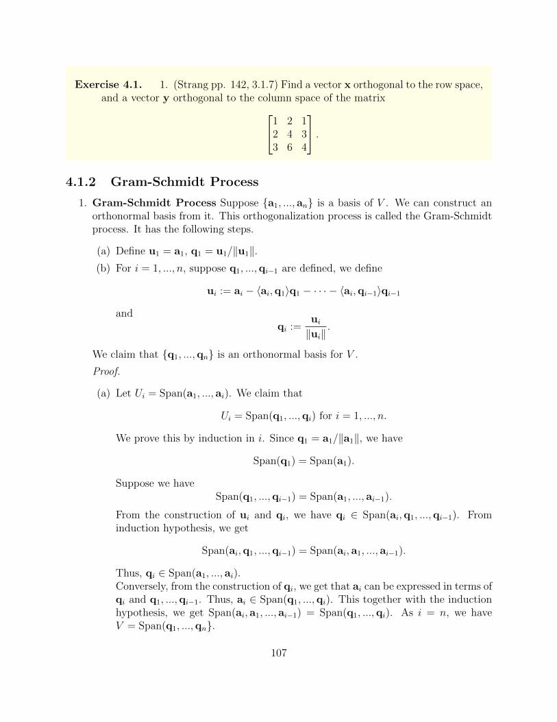
Exercise 4.1. 1. (Strang pp. 142, 3.1.7) Find a vector x orthogonal to the row space,and a vector y orthogonal to the column space of the matrix1 2 1
2 4 33 6 4
.4.1.2 Gram-Schmidt Process
1. Gram-Schmidt Process Suppose a1, ..., an is a basis of V . We can construct anorthonormal basis from it. This orthogonalization process is called the Gram-Schmidtprocess. It has the following steps.
(a) Define u1 = a1, q1 = u1/‖u1‖.(b) For i = 1, ..., n, suppose q1, ...,qi−1 are defined, we define
ui := ai − 〈ai,q1〉q1 − · · · − 〈ai,qi−1〉qi−1
andqi :=
ui‖ui‖
.
We claim that q1, ...,qn is an orthonormal basis for V .
Proof.
(a) Let Ui = Span(a1, ..., ai). We claim that
Ui = Span(q1, ...,qi) for i = 1, ..., n.
We prove this by induction in i. Since q1 = a1/‖a1‖, we have
Span(q1) = Span(a1).
Suppose we haveSpan(q1, ...,qi−1) = Span(a1, ..., ai−1).
From the construction of ui and qi, we have qi ∈ Span(ai,q1, ...,qi−1). Frominduction hypothesis, we get
Span(ai,q1, ...,qi−1) = Span(ai, a1, ..., ai−1).
Thus, qi ∈ Span(a1, ..., ai).Conversely, from the construction of qi, we get that ai can be expressed in terms ofqi and q1, ...,qi−1. Thus, ai ∈ Span(q1, ...,qi). This together with the inductionhypothesis, we get Span(ai, a1, ..., ai−1) = Span(q1, ...,qi). As i = n, we haveV = Span(q1, ...,qn.
107

(b) Given i = 2, ..., n, we show ui ⊥ qj for j < i.
〈ui,qj〉 = 〈ai −i−1∑k=1
〈ai,qk〉qk,qj〉
= 〈ai,qj〉 −i−1∑k=1
〈ai,qk〉δkj
= 〈ai,qj〉 − 〈ai,qj〉 = 0.
Since qi = ui/‖ui‖, we thus have qi ⊥ Ui−1 for i = 2, ..., n. This shows q1, ...,qnis orthonormal.
2. Example 1: Let
A = [a1, a2, a3] =
1 1 01 0 10 1 1
We perform Gram-Schmidt orthonormal process:
u2 = a2 −1
‖a1‖2〈a2, a1〉a1
= [1, 0, 1]T − 1
2[1, 1, 0]T = [
1
2,−1
2, 1]T .
u3 = a3 −1
‖a1‖2〈a3, a1〉a1 −
1
‖u2‖2〈a3,u2〉u2
= [0, 1, 1]T − 1
2[1, 1, 0]T − 2
3
1
2[1
2,−1
2, 1]T
=2
3[−1, 1, 1]T .
After normalization, we get
q1 =1√2
110
, q2 =1√6
1−12
, q3 =1√3
−111
.3. Example 2. Legendre polynomials. In the function space C[−1, 1], we define the inner
product by
〈f, g〉 :=
ˆ 1
−1
f(x)g(x) dx.
For polynomials 1, x, x2, ..., xn, we perform Gram-Schmidt procedure to get the Leg-endre polynomial p`. Let us construct few of them.
108

• ` = 0, we start with p0(x) ≡ 1.
• ` = 1, we find 〈x, 1〉 = 0. Thus, we choose p1(x) = x.
• ` = 2, the Gram-Schmidt orthogonalization gives
p2(x) = x2 − 〈x2, 1〉〈1, 1〉
1− 〈x2, x〉〈x, x〉
x = x2 − 1
3.
• For ` = 3, instead of performing Gram-Schmidt process on x3, we apply thisprocess on xp2(x):
p3(x) = xp2(x)− 〈xp2, p2〉〈p2, p2〉
p2(x)− 〈xp2, p1〉〈p1, p1〉
p1(x)− 〈xp2, p0〉〈p0, p0〉
p0
The advantage is that the last term is zero because
〈xp2, p0〉 = 〈p2, xp0〉 = 0, ∵ xp0 is of degree 1.
The calculation gives
p3(x) = x3 − 3
5x.
• In general, suppose we have found p0, ..., pn, we obtain pn+1 by
pn+1(x) = xpn(x)− 〈xpn, pn〉〈pn, pn〉
pn(x)− 〈xpn, pn−1〉〈pn−1, pn−1〉
pn−1(x)−n−2∑j=0
〈xpn, pj〉〈pj, pj〉
pj(x).
The last terms are all zeros:
〈xpn, pj〉 = 〈pn, xpj〉 = 0 for 0 ≤ j ≤ n− 2
because xpj is a polynomial of degree j+1 which is orthogonal to pn for j ≤ n−2.Thus,
pn+1(x) = xpn(x)− 〈xpn, pn〉〈pn, pn〉
pn(x)− 〈xpn, pn−1〉〈pn−1, pn−1〉
pn−1(x).
• The polynomials pn are orthogonal to each other. The standard Legendre poly-nomial Pn(x) is a normalization of pn by
Pn(x) = cnpn(x)
The constant cn is chosen such that
Pn(1) = 1.
By a direct calculation of the coefficients of pn, one can obtain
cn =(2n)!
2n(n!)2.
109

• The standard Legendre polynomial Pn satisfies an easier recurrence relation:
(n+ 1)Pn+1(x) = (2n+ 1)xPn(x)− nPn−1(x).
And the orthogonal property
〈Pn, Pm〉 =2
2n+ 1δm,n.
4. QR decomposition
(a) Let A = [a1, ..., an] be an n × n matrix. The Gram-Schmidt orthogonalizationprocess constructs q1, ...,qn such that
Span(q1, ...,qi) = Span(a1, ..., ai), i = 1, ..., n.
q1, ...,qn is orthonormal.
Thus, we can express ai in terms of qj as
ai =n∑j=1
〈ai,qj〉qj =i∑
j=1
〈ai,qj〉qj. (∵ qj ⊥ Span(a1, ..., ai) for j > i)
In matrix form, it reads
A = QR, Q = [q1, ...,qn], R =
〈a1,q1〉 〈a2,q1〉 · · · 〈an,q1〉
0 〈a2,q2〉 · · · 〈an,q2〉...
. . ....
0 0 · · · 〈an,qn〉
.This is called a QR decomposition of a matrix A. In our early example,
A =
1 1 01 0 10 1 1
, Q =
1√2
1√6− 1√
31√2− 1√
61√3
0 2√6
1√3
, R =
√
2 1√2
1√2
0√
3√2
1√6
0 0√
3
.(b) Suppose A = [a1, ..., an] is an m× n matrix and m < n. Then the QR decompo-
sition has the formA = Qm×mRm×n.
The upper triangular matrix R is a fat matrix.
5. Application of QR decomposition. Usually, QR decomposition is used for computingdeterminant or eigenvalues/eigenvectors. Here, we will use it to solve the linear system
Ax = b.
110

For the case m ≤ n, we assume A is of full rank. That is, rank(A) = m. As A isdecomposed in QR form, the equation Ax = b becomes
QRx = b.
Since Q−1 = QT , this equation is equivalent to
Rx = QTb.
The inversion of R can be solved by backward substitution.
Exercise 4.2. 1. (Strang pp. 181, 3.4.13) Apply the Gram-Schmidt process to
a1 =
001
, a2 =
011
, a3 =
111
,and write the result in A = QR form.
2. (Strang pp. 181, 3.4.15) Find an orthonormal set q1,q2,q3 for which q1,q2 spanthe column space of
A =
1 12 −1−2 4
.What is the fundamental subspace of A contains q3? What is the least-squaressolution of Ax = b if b = [1, 2, 7]T ?
4.2 Orthogonal Projection
4.2.1 Orthogonal Projection operators
1. Given a subspace Z ⊂ W , we would like to construct a linear map PZ : W → Z suchthat
PZb ∈ Z, and (b− PZb) ⊥ Z for all b ∈ W.
Such an operator is called the orthogonal projection operator onto Z.
2. Case 1, Z = Span(a). We have seen that we can decompose another vector b into twoparts
b = b‖ + b⊥,
where
b‖ =b · aaTa
a, b⊥ = b− b‖, b‖ ⊥ b⊥.
111

We call b‖ the projection of b onto a. In terms of operator, it is
Pa(b) =1
aTaaaTb.
For example, a = [1, 2,−1]T ∈ R3, the matrix representation for the projection operatorPa is
Pa =1
aTaaaT =
1
6
12−1
[1 2 −1]
=1
6
1 2 −12 4 −2−1 −2 1
3. Case 2, Z = Span(a1, a2). We assume a1, a2 is independent. The projection operator
is PZ(b) = b‖, with b‖ ∈ Z and b− b‖ ⊥ Z. To find b‖, we set
b‖ = x1a1 + x2a2.
From b− b‖ ⊥ Z, we get two equations
〈b− b‖, ai〉 = 0, i = 1, 2.
This gives two equations 〈a1, a1〉x1 + 〈a1, a2〉x2 = 〈a1,b〉〈a2, a1〉x1 + 〈a2, a2〉x2 = 〈a2,b〉
for x1, x2. Its solution can be obtained by[x∗1x∗2
]=
[〈a1, a1〉 〈a1, a2〉〈a2, a1〉 〈a2, a2〉
]−1 [〈a1,b〉〈a2,b〉
].
We note that [〈a1, a1〉 〈a1, a2〉〈a2, a1〉 〈a2, a2〉
]= ATA,
[〈a1,b〉〈a2,b〉
]= ATb.
Thus,x∗ = (ATA)−1ATb.
The projection operator
PZ(b) = b‖ = x∗1a1 + x∗2a2 = Ax∗ = A(ATA)−1ATb.
Example Suppose
A =
1 12 00 −1
.We consider the problem
Ax = b.
112

The least-squares solution is the solution x∗ which solves the normal equation
ATAx∗ = ATb.
Since u1,u2 is independent, we get that ATA is non-singular and x∗ = (ATA)−1Ab.The projection of b onto Span(u1,u2) is
PZ = A(ATA)−1AT .
In this example,
ATA =
[1 2 01 0 −1
]1 12 00 −1
=
[5 11 2
]
PZ = A(ATA)−1AT =
1 12 00 −1
[5 11 2
]−1 [1 2 01 0 −1
]
=1
9
1 12 00 −1
[ 2 −1−1 5
] [1 2 01 0 −1
]=
1
9
5 2 −42 8 2−4 2 5
4. Alternatively, we can apply the Gram-Schmidt orthogonalization on a1, a2. This
gives u1,u2 with u2 ⊥ u1. Suppose b‖ = y1u1+y2u2. Then the condition b−b‖ ⊥ Zgives
〈u1,u1〉y1 = 〈u1,b〉〈u2,u2〉y2 = 〈u2,b〉
.
We get
PZ(b) = y1u1 + y2u2 =〈u1,b〉〈u1,u1〉
u1 +〈u2,b〉〈u2,u2〉
u1
=
(1
〈u1,u1〉u1u
T1 +
1
〈u2,u2〉u2u
T2
)b.
Now in the above exampleA = [a1, a2].
Let us perform Gram-Schmidt orthogonalization to the column vectors of A to get
u1 =
120
, u2 =
45
−25
−1
The projection operator is given by
PZ =1
5u1u
T1 +
1
9/5u2u
T2
113
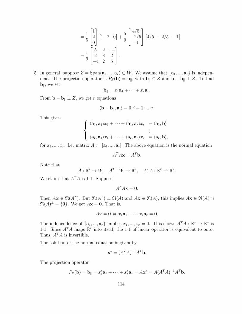
=1
5
120
[1 2 0]
+5
9
4/5−2/5−1
[4/5 −2/5 −1]
=1
9
5 2 −42 8 2−4 2 5
.5. In general, suppose Z = Span(a1, ..., ar) ⊂ W . We assume that a1, ..., ar is indepen-
dent. The projection operator is PZ(b) = b‖, with b‖ ∈ Z and b − b‖ ⊥ Z. To findb‖, we set
b‖ = x1a1 + · · ·+ xrar.
From b− b‖ ⊥ Z, we get r equations
〈b− b‖, ai〉 = 0, i = 1, ..., r.
This gives 〈a1, a1〉x1 + · · ·+ 〈a1, ar〉xr = 〈a1,b〉
...〈ar, a1〉x1 + · · ·+ 〈ar, ar〉xr = 〈ar,b〉,
for x1, ..., xr. Let matrix A := [a1, ..., ar]. The above equation is the normal equation
ATAx = ATb.
Note thatA : Rr → W, AT : W → Rr, ATA : Rr → Rr.
We claim that ATA is 1-1. Suppose
ATAx = 0.
Then Ax ∈ N(AT ). But N(AT ) ⊥ R(A) and Ax ∈ R(A), this implies Ax ∈ R(A) ∩R(A)⊥ = 0. We get Ax = 0. That is,
Ax = 0⇔ x1a1 + · · ·xrar = 0.
The independence of a1, ..., ar implies x1, ..., xr = 0. This shows ATA : Rr → Rr is1-1. Since ATA maps Rr into itself, the 1-1 of linear operator is equivalent to onto.Thus, ATA is invertible.
The solution of the normal equation is given by
x∗ = (ATA)−1ATb.
The projection operator
PZ(b) = b‖ = x∗1a1 + · · ·+ x∗rar = Ax∗ = A(ATA)−1ATb.
114

6. The orthogonal projection P satisfies
P 2 = P = P T .
This can be seen from
P T = (A(ATA)−1AT )T = A(ATA)−TAT = A(ATA)−1AT = P.
To show P 2 = P ,
P 2 = (A(ATA)−1AT )(A(ATA)−1AT ) = A(ATA)−1(ATA)(ATA)−1AT = A(ATA)−1AT = P.
7. Conversely, suppose an operator P : W → W satisfies P 2 = P = P T , then it is anorthogonal projection operator. To show this, we define Z := R(P ), and choose a basisa1, ..., ar for Z. Let A = [a1, ..., ar]. Then we claim that P = PZ .
Proof. (Hint) You can decompose W = Z ⊕ Z⊥. For any b ∈ W , b = b‖ + b⊥ withb‖ ∈ Z and b⊥ ∈ Z⊥. Then show Pb = b‖.
4.3 Least-squares method
4.3.1 Least-squares method for a line fitting
1. In statistical analysis, a regression model is to link dependent variables to independentvariables through a set of data. The data look like (X1, Y1), ..., (Xn, Yn). A linearregression model has the form
y = β0 + β1x+ η,
where x is the independent variable, y the dependent variable, η the error, ∗ and β0, β1
the parameters to be determined. If there is no error, then we would get
β0 +Xiβ1 = Yi, i = 1, ..., N.
In matrix formAβ = Y, (4.1)
where
A =[1 X
], β =
[β0
β1
], 1 =
1...1
, X =
X1...XN
, Y =
Y1...YN
.Equation 4.1 is an over-determined system when N > 2. In general, there is no solutionfor (β0, β1) unless Y ⊥ N(AT ). Thus, we should allow errors in the data in order tohave a suitable solution.
∗η is a random variable. Different sampling may give different error.
115

2. A regression process is to determine the parameters β0 and β1 so that the model is bestfit to the data. One way is to minimize the total error
E(β0, β1) :=1
2
N∑j=1
(Yj − (β0 + β1Xj))2 . (4.2)
If (β∗0 , β∗1) is the minimal solution, it satisfies
∂E
∂β0
(β∗0 , β∗1) =
N∑j=1
(β∗0 + β∗1Xj − Yj) = 0
∂E
∂β1
(β∗0 , β∗1) =
N∑j=1
(β∗0 + β∗1Xj − Yj)Xj = 0.
In matrix form, it reads [〈1,1〉 〈1,X〉〈1,X〉 〈X,X〉
] [β∗0β∗1
]=
[〈1,Y〉〈X,Y〉
]. (4.3)
When it is expressed in terms of A = [1,X], it reads
ATAβ∗ = ATY.
This is called the normal equation corresponding the original over-determined system.It is solvable if the column vectors of A are independent. Its solution is given by
β∗0 =
∣∣∣∣ 〈1,Y〉 〈1,X〉〈X,Y〉 〈X,X〉
∣∣∣∣∣∣∣∣ 〈1,1〉 〈1,X〉〈1,X〉 〈X,X〉
∣∣∣∣ , β∗1 =
∣∣∣∣ 〈1,1〉 〈1,Y〉〈1,X〉 〈X,Y〉
∣∣∣∣∣∣∣∣ 〈1,1〉 〈1,X〉〈1,X〉 〈X,X〉
∣∣∣∣ .The solution (β∗0 , β
∗1) is called the least-squares solutions for (4.1) because it minimizes
the total squares of the errors (4.2).
3. Now, we take the point of view of orthogonal projection for the above least-squaressolutions. Recall that the matrix A = [1,X] is a linear transformation from R2 to RN .The over-determined system Aβ = Y has a solution only when Y ∈ R(A). In the casewhen Y 6∈ R(A), we project Y to R(A) in order to find a best fit solution. We claimthat Aβ∗, with β∗ being the least-squares solution, is the orthogonal projection of Yon R(A). This is the Theorem 4.1 below.
4. Example (Strang’s pp. 161). The data set is (−1, 1), (1, 1), (2, 3). We look for a liney = β0 + β1x that best fits to these data. The equation for exact fitting is1 −1
1 11 2
[β0
β1
]=
113
.116

The corresponding normal equation is ATAβ = ATY:
[1 1 1−1 1 2
]1 −11 11 2
[β∗0β∗1
]=
[1 1 1−1 1 2
]113
⇒[3 22 6
] [β∗0β∗1
]=
[56
]
This gives
β∗0 =9
7, β∗1 =
4
7.
The vector Aβ∗ = [5/7, 13/7, 17/7]T is the projection of Y = [1, 1, 3] onto the columnspace R(A).
5. We can express the normal equation in a saddle form. Recall that our regression modelis
Y = Aβ + η.
Here, η is the error. It is an N -by-1 column matrix. The normal equation is
AT (Aβ −Y) = 0.
Combine these two, we getATη = 0.
Thus, the least-squares solution β∗ and the corresponding error η∗ satisfy[I AAT 0
] [η∗
β∗
]=
[Y0
]. (4.4)
†
6. Weighted least-squares method In general, we consider weighted least-squaresmethod which minimizes the weighted errors
Ew(β0, β1) :=1
2
N∑j=1
wj (Yj − (β0 + β1Xj))2 , (4.6)
where wj > 0, j = 1, ..., N are the weights. The minimum (β∗0 , β∗1) satisfies
∂E
∂β0
(β∗0 , β∗1) =
N∑j=1
wj(β∗0 + β∗1Xj − Yj) = 0
†We may compare this equation with the equation appeared in Chapter 1[C−1 AAT 0
] [wu
]=
[fg
]. (4.5)
Such kinds of equations appear commonly in various fields.
117

∂E
∂β1
(β∗0 , β∗1) =
N∑j=1
wj(β∗0 + β∗1Xj − Yj)Xj = 0.
In matrix form, it is [〈1,1〉w 〈1,X〉w〈1,X〉w 〈X,X〉w
] [β∗0β∗1
]=
[〈1,Y〉w〈X,Y〉w
]. (4.7)
Here, the weighted inner product 〈·, ·〉w is defined as
〈a,b〉w :=n∑j=1
wjajbj.
One can show that 〈·, ·〉w is an inner product when w’s are positive. The normalequation becomes
ATWAβ∗ = WY.
where
W =
[w1
w2
]is called the weighted matrix. As we express this normal equation in saddle form, it is[
W−1 AAT 0
] [η∗
β∗
]=
[Y0
]. (4.8)
The weighted matrix W is indeed the correlation matrix of the random error η.
Exercise 4.3. 1. Suppose we are given data (1, 3), (2, 5), (3, 6), (4, 7). We look for alinear model
y = β0 + β1x+ η
such that the error
E(β0, β1) =1
2[(β0 + β1 − 3)2 + (β0 + 2β1 − 5)2 + (β0 + 3β1 − 6)2 + (β0 + 4β1 − 7)2]
is the smallest. Find best β0 and β1.
2. (Strang pp. 165, 3.3.4) Find the best straight line fit to the following measurements:(xi, yi) are
(−1, 2), (0, 0), (1,−3), (2,−5).
3. (Strang pp. 165, 3.3.5) For the above data, we want to fit them to a parabola:y = a2x
2 + a1x+ a0. What are the best fit coefficients if you want to have a leastsquares errors.
118

4. Consider a measurement on the plane, we obtain Y = 2, 3, 4, 5 respectively at grids(X1, X2) = (1, 1), (1, 2), (2, 1), (2, 2). Find a least-squares solution for a plane-fitfor these data. That is, the regression model is
y = β0 + β1x1 + β2x2 + η.
5. (Strang 209, 3.33)
(a) Find an orthonormal basis for the column space of
A =
1 −63 64 85 07 8
(b) Find QR decomposition of A.
(c) Find the least-squares solution of Ax = b for b = [−3, 7, 1, 0, 4]T .
6. Find the curve y = C +D2x which gves the best least squares fit to the measure-ments (xi, yi) = (0, 6), (1, 4), (2, 0).
4.3.2 Least-squares method for general linear systems
1. The above procedure can be generalized to curve fitting, surface fitting, and moregeneral statistical models for fitting a data set. A measurement model is usuallyexpressed as
Ax = b + η.
where A is called the measurement matrix, b the measured data, η the measurementerrors. The unknowns x are the parameters we look for. Usually, the number ofparameters and number of measurements may not be the same. Secondly, b may notbe in R(A) and thus may lead to no solution. Thirdly, small perturbation of b maylead to big change of the parameters. This kind of data fitting is not robust. Thus, welook for the least-squares solution with minimum norm. This is to solve
minx‖Ax− b‖2
and with minimal ‖x‖2.
2. For the least-squares solutions, we have the following theorem.
Theorem 4.1. The solution x∗ which satisfies
‖Ax∗ − b‖2 ≤ ‖Az− b‖2 for all z ∈ V
119

if and only if x∗ satisfies the normal equation:
ATAx∗ = ATb.
Proof. Note that
ATAx = ATb⇔ AT (Ax∗ − b) = 0⇔ Ax∗ − b ∈ N(AT )⇔ Ax∗ − b ⊥ R(AT ).
Suppose AT (Ax∗ − b) = 0. For any z ∈ V ,
Az− b = A(z− x∗) + (Ax∗ − b).
This is an orthogonal decomposition: the first term is in R(A), the second term isperpendicular to R(A). Thus,
‖Az− b‖2 = ‖A(z− x∗)‖2 + ‖Ax∗ − b‖2 ≥ ‖Ax∗ − b‖2.
Conversely, if y∗ ∈ R(A) with ‖y∗ − b‖ having the shortest distance to R(A), theny∗ − b ⊥ R(A). This implies AT (y∗ − b) = 0.
3. Next, we analyze the solution structure for the normal equation: ATAx = b. SupposeA =
[a1 · · · an
]. Then
ATA =
a1 · a1 · · · a1 · an...
. . ....
an · a1 · · · an · an
.The mapping ATA : V → V . Since R(AT ) ⊂ V is a subspace. We also noticethat R(ATA) ⊂ R(AT ). We can restrict ATA to the subspace R(AT ). Denote thisrestrxicted mapping by ATA|R(AT ).
Proposition 4.2. (a) N(ATA) = N(A),
(b) R(ATA) = R(AT )
(c) The mapping ATA|R(AT ) : R(AT )→ R(AT ) is 1-1 and onto.
Proof. (a) If ATAx = 0, then xT (ATAx) = 0. This is ‖Ax‖2 = 0. Hence Ax = 0.We get x ∈ N(A). Hence N(ATA) ⊂ N(A). The other side is trivial.
(b) R(ATA) ⊂ R(AT ) is trivial. The other side follows from (c). Alternatively, weprove directly. For any b ∈ W , it can be decomposed into b = b‖ + b⊥ withb‖ ∈ R(A) and b⊥ ∈ N(AT ). For b‖ ∈ R(A), there exists v ∈ V such thatAv = b‖. Thus, we get
ATb = AT (b‖ + b⊥) = ATAv ∈ R(ATA).
120

(c) We show that the restricted mapping is 1-1, or equivalently
N(ATA|R(AT )) = N(ATA) ∩R(AT ) = 0.
This follows from N(ATA) = N(A) and R(AT )⊥ = N(A).
Next, The onto part of ATA|R(AT ) follows from the fundamental theorem of linearmap, which gives
dimR(AT ) = dimR(ATA|R(AT )) + dimN(ATA|R(AT )) = dimR(ATA).
Since R(ATA) ⊂ R(AT ), we conclude that R(ATA) = R(AT ).
4. For the minimal norm solution among all least-squares solutions, we have the followingtheorem.
Theorem 4.2. (a) The general form of the least-squares solution of Ax = b hasthe expression:
xlsq = x∗ + xnull, with xnull ∈ N(A).
where x∗ is the least-squares solution that lies in R(AT ).
(b) x∗ is the least-squares solution with minimal norm.
Proof. (a) From Theorem 4.1, we have that the least-squares solution satisfies thenormal equation ATAx = ATb.
(b) From Proposition 4.2, the solution of the normal equation has the form
x∗ + N(ATA) = x∗ + N(A),
where
x∗ =(ATA|R(AT )
)−1(ATb). (4.9)
(c) Since x∗ ∈ R(AT ) which is orthogonal to N(A), we have that
‖x∗‖ ≤ ‖xlsq‖.
Thus, among all least-square solutions, the particular solution x∗ has the leastnorm. That is, x∗ is the least-squares solution with least norm.
121

5. Remark. This particular solution x∗ is usually denoted by A+b, and is called theMoore-Penrose pseudo inverse of A. That is,
A+ :=(ATA|R(AT )
)−1AT .
It satisfies A+Ax = x, when A is invertible. We will see in Chapter 5 that
A+A = PR(AT ), AA+ = PR(A).
6. Example Consider the following measurement matrix and data:
A =
1 −1 2 00 1 −1 11 0 1 1
, b =
133
.We look for a least-squares solution with minimal norm.
Hint. The normal equation ATAx = ATb is2 −1 3 1−1 2 −3 13 −3 6 01 1 0 2
x1
x2
x3
x4
=
4226
You can check that
N(A) = Span(
−1110
,−1−101
).
Find a special solution, then among all least-squares solution find the one which isperpendicular to N(A).
Exercise 4.4. 1. (Strang pp. 451) What is the minimum length least squares solutionx∗ = A+b to
Aa =
1 0 01 0 01 1 1
a0
a1
a2
=
022
?
This problem fits the best plane y = a0+a1x1+a2x2 to the data points (x1, x2, y) =(0, 0, 0), (0, 0, 2), (1, 1, 2).
2. (Strang pp. 452 A.6)
(a) If A has independent columns, its left-inverse (ATA)−1AT is its pseudoinverse.
122

(b) (Strang pp. 452 A.6) If A has independent rows, its right-inverse AT (AAT )−1
is its pseudoinverse.
(c) In both cases, verify A+b ∈ R(AT ) and ATAx∗ = ATb.
123

124

Chapter 5
Determinant
5.1 Determinant of matrices
5.1.1 Determinant as a signed volume
1. Given an n× n matrix A, its determinant is defined to measure the signed volume ofthe parallelotope ∗ spanned by its column vectors. We will show later that it is alsoequal to the signed volume of the parallelotope spanned by its its row vectors. Suppose
A =[a1 · · · an
],
the determinant of A is denoted by
det(A) = det (a1, ..., an) =
∣∣∣∣∣∣∣a11 · · · a1n...
. . ....
an1 · · · ann
∣∣∣∣∣∣∣ .2. The determinant function is required to satisfy the following properties:
(a) The determinant changes sign if we exchange two columns:
det (a1, · · · , aj, · · · , ai, · · · , an) = − det (a1, · · · , ai, · · · , aj, · · · , an) .
For instance, in two dimensions,
det(e2, e1) = − det(e1, e2).
It means that the signed area of (a2, a1) is the negative of the signed area of(a1, a2). The orientation of (a1, a2) matters. In three dimensions,
det(e2, e1, e3) = det(e1, e3, e2) = det(e3, e2, e1) = − det(e1, e2, e3),
∗It is called the parallelogram in 2D, parallelelepiped in 3D, and parallelotope in high dimensions.
125

anddet(e2, e3, e1) = det(e3, e1, e2) = det(e1, e2, e3).
In the first example, there is only one column exchange. In the second example,there are two column exchanges, therefore the sign is changed back.As a consequence this property, the determinant is zero if there are two equalcolumns.
(b) The determinant is linear in each column vector:
det(a1, · · · , a1
i + a2i , · · · , an
)= det
(a1, · · · , a1
i , · · · , an)+det
(a1, · · · , a2
i , · · · , an)
det (a1, · · · , αai, · · · , an) = α det (a1, · · · , ai, · · · , an)
Here is the graphic explanation of this property in two dimensions.
(c) The determinant of the volume spanned by the standard basis e1, ..., enis 1:
det(e1, · · · , en) = 1.
3. We will show that the determinant function satisfying the above three properties doesexist, and has an exact expression. Let us study the expression of determinant in 2Dand 3D first.
(a) In 2D,
det(a1, a2) = det(a11e1 + a21e2, a12e1 + a22e2)
= a11a12 det(e1, e1) + a11a22 det(e1, e2)
+ a21a12 det(e2, e1) + a21a22 det(e2, e2)
= a11a22 det(e1, e2) + a21a12 det(e2, e1)
= (a11a22 − a21a12) det(e1, e2)
= a11a22 − a21a12.
(b) In 3D, we have
det(a1, a2, a3) = det
(3∑
j1=1
a1,j1ej1 ,3∑
j2=1
a2,j2ej2 ,3∑
j3=1
a3,j3ej3
)
=3∑
j1=1
3∑j2=1
3∑j3=1
a1,j1a2,j2a3,j3 det(ej1 , ej2 , ej3)
Now, det(ej1 , ej2 , ej3) = 0 if two of j1, j2, j3 are equal. Let us rename j1, j2, j3by σ1, σ2, σ3. The index function σ is a mapping from 1, 2, 3 to itself. It hasto be 1-1 and onto, otherwise the corresponding det(eσ1 , eσ2 , eσ3) = 0. Suchan index function is called a permutation. We denote it by the ordered tupleσ = (σ1, σ2, σ3). For instance, σ = (3, 1, 2) means that (σ1, σ2, σ3) = (3, 1, 2), or
126

σ : 1, 2, 3 → 1, 2, 3 with σ(1) = 3, σ(2) = 1 and σ(3) = 2. There are 3! per-mutations of the set 1, 2, 3. They are (1, 2, 3), (2, 3, 1), (3, 1, 2), (2, 1, 3), (1, 3, 2)and (3, 2, 1). The determinant of det(eσ1 , eσ2 , eσ3) can be changed to the normalone det(e1, e2, e3) by using property (a):
det(e2, e1, e3) = det(e3, e2, e1) = det(e1, e3, e2) = − det(e1, e2, e3).
det(e2, e3, e1) = − det(e2, e1, e3) = det(e1, e2, e3)
det(e3, e1, e2) = − det(e1, e3, e2) = det(e1, e2, e3)
Thus, the determinant of a 3× 3 matrix is
det(a1, a2, a3) =3∑
j1=1
3∑j2=1
3∑j3=1
a1,j1a2,j2a3,j3 det(ej1 , ej2 , ej3)
= a11a22a33 + a12a23a31 + a13a21a32
− a13a22a31 − a11a23a32 − a12a21a33.
(c) In general, the set of all permutations of (1, 2, ..., n) forms a group under functioncomposition. It is denoted by Sn.
Sn := σ : 1, ..., n → 1, ..., n 1-1 and onto.
The multiplication of two permutations σ, τ ∈ Sn is defined as
(στ)(i) = τ(σ(i)).
For instance, σ = (1, 3, 2), τ = (3, 1, 2) ∈ S3. We have
σ : 1 7→ 1, 2 7→ 3, 3 7→ 2,
τ : 1 7→ 3, 2 7→ 1, 3 7→ 2,
στ : 1 7→ 1 7→ 3, 2 7→ 3 7→ 2, 3 7→ 2 7→ 1.
Thus, (1, 3, 2)(3, 1, 2) = (3, 2, 1). Sn with function composition forms a group.The number of Sn = n!.
A transposition of a permutation σ is a pair (j, i) with i < j such that i appearsafter j in (σ1, ..., σn). A permutation is called even (resp. odd) if it has even(resp. odd) number of transpositions. The sign of a permutation σ is defined by
sign(σ) =
1 if σ is an even permutation−1 if σ is an odd permutation.
For example, (1, 3, 2) has one transposition (3, 2). Thus, it is an odd permutation.Whereas (2, 3, 1) has two transpositions (2, 1), (3, 1). It is an even permutation.Note that an even (resp. odd) permutation can be expressed as a composition ofeven (resp. odd) number transpositions. Thus, we have
det(eσ1 , · · · , eσn) = sign(σ) det(e1, · · · , en).
We conclude with the following theorem.
127

Theorem 5.1. The determinant function det(a1, · · · , an) exists and has the fol-lowing expression
det(A) =∑σ∈Sn
sign(σ)a1,σ1 · · · an,σn . (5.1)
Here, the summation is over all permutations σ : 1, ..., n → 1, ..., n.
4. det(A) = 1n!
∑σ,τ sign(σ)sign(τ)aτ1,σ1 · · · aτn,σn .
Exercise 5.1. 1 In R4, what is the signed volume of the hypercubes:
det(e1, e4, e2, e3), det(e3, e1, e2, e4), det(e2, e3, e4, e1).
2 (Schaum pp. 122) Find the signs of the following permutations in S5 and S6:
σ = (2, 1, 3, 5, 4), (3, 1, 2, 4, 5), (5, 2, 1, 3, 4); (5, 4, 2, 1, 6, 3).
3 (Schaum pp. 122) Find τ σ in S5, where
σ = (2, 4, 5, 1, 3), τ = (4, 1, 3, 5, 2).
4 Find the determinants of the following two matrices:
A1 =
0 0 0 10 0 1 00 1 0 01 0 0 0
, A2 =
0 1 0 00 0 1 00 1 0 01 0 0 0
5.1.2 Properties of determinant
1. The determinant is also a measure of signed volume of the palallelotope spanned bythe row vectors.
Theorem 5.2. Suppose A has column vectors (a1, ..., an) and row vectors (A1, ...,An).Then
det(A1, ...,An) = det(a1, ..., an).
In other words,det(AT ) = det(A). (5.2)
Proof. Every permutation σ is 1-1 and onto, thus invertible. Let us denote its inverseby σ−1. You can check that
sign(σ−1) = sign(σ).
128

Then the determinant formula (5.1) can be expressed as
det(A) =∑σ
sign(σ)a1,σ1 · · · an,σn
=∑σ
sign(σ)aσ−11 ,1 · · · aσ−1
n ,n
=∑σ
sign(σ−1)aσ−11 ,1 · · · aσ−1
n ,n
=∑τ
sign(τ)aτ1,1 · · · aτn,n
= det(AT ) = det(A1, ...,An).
2. Product rule: det is multiplicative:
Theorem 5.3 (Product rule). The determinant is multiplicative:
det(AB) = det(A) det(B). (5.3)
Proof. Let us write B = [b1, ...,bn].
det(AB) = det(Ab1, ..., Abn)
= det
(A
n∑i1
bi1,1ei1 , ..., An∑in
bin,nein
)
=n∑
i1=1
· · ·n∑
in=1
bi1,1 · · · bin,n det (Aei1 , ..., Aein)
=∑
(i1,··· ,in)
bi1,1 · · · bin,nsign(i1, · · · , in) det(Ae1, ..., Aen)
= det(BT ) det(A) = det(B) det(A).
As a corollary,
det(A−1) = det(A)−1.
3. The determinant of an upper triangular matrix A is the product of its diagonal terms.∣∣∣∣∣∣∣∣∣a11 a12 · · · a1n
0 a22 · · · a2n...
. . . . . ....
0 · · · 0 ann
∣∣∣∣∣∣∣∣∣ = a11 · · · ann.
129

Proof. The upper triangular matrix A has the property:
aij = 0, for all i > j.
In the determinant formula (5.1), only the natural permutation σ = (1, 2, ..., n) satisfiesσi = i for all i = 1, ..., n. The rest σ has at least one i satisfying i > σi. This leads toai,σi = 0, because A is upper triangular. Thus,
det(A) =∑σ
sign(σ)a1,σ1 · · · an,σn = a11 · · · ann.
4. Properties (a) and (b) imply that the determinant is unchanged under shearing columnoperations or shearing row operations:
det(a1, ..., ai, ..., aj + αai, ..., an) = det(a1, ..., ai, ..., aj, ..., an) + α det(a1, ..., ai, ..., ai, ..., an)
= det(a1, ..., ai, ..., aj, ..., an),
det
AT1
...ATi
...ATj + αAT
i...
ATn
= det
AT1
...ATi
...ATj
...ATn
+ α det
AT1
...ATi
...ATi
...ATn
= det
AT1
...ATi
...ATj
...ATn
.
5. Examples Use row operations to compute det(A).
(a) ∣∣∣∣∣∣1 −1 20 1 −2−1 0 −1
∣∣∣∣∣∣ =
∣∣∣∣∣∣1 −1 20 1 −20 −1 1
∣∣∣∣∣∣ =
∣∣∣∣∣∣1 −1 20 1 −20 0 −1
∣∣∣∣∣∣ = −1.
(b) ∣∣∣∣∣∣1 2 20 5 −21 −3 4
∣∣∣∣∣∣ =
∣∣∣∣∣∣1 2 20 5 −20 −5 2
∣∣∣∣∣∣ = 0
(c) Let
det(A) =
∣∣∣∣cos(θ) − sin(θ)sin(θ) cos(θ)
∣∣∣∣ = 1.
In general, let R be a rotational matrix, i.e. RTR = I. Then
1 = det(RTR) = det(R)2.
Thus, det(R) = ±1.
130

6. We can use Gaussian elimination to compute detA: From Gaussian elimination, A =LU (1.9):
a11 a12 a13 · · · a1n
a21 a22 a23 · · · a2n
a31 a32 a33 · · · a3n...
. . .
an1 an2 an3 · · · ann
=
1 0 0 · · · 0`21 1 0 · · · 0`31 `32 1 · · · 0
.... . .
`n1 `n2 `n3 · · · 1
u11 u12 u13 · · · u1n
0 u22 u23 · · · u2n
0 0 u33 · · · u3n...
. . .
0 0 0 · · · unn
Then
detA = det(L) det(U) = det(U) = u11 · · ·unn.
7. Determinant and Singularity
• Properties (a) and (b) implies that det(A) = 0 if a1, ..., an is linearly dependent⇔ R(A) is not onto ⇔ A is singular.
• Recall that the echelon form of a matrix A is an upper triangular matrix U . Therow vectors of U constitute a basis for R(AT ). Thus,
R(AT ) = Rn ⇔ (uii 6= 0 for all i = 1, ...n)⇔ detA 6= 0.
But R(AT ) = Rn is equivalent to R(A) = Rn. Thus, A is onto. This is againequivalent to A is nonsingular.
This shows the following theorem:
Theorem 5.4. Let A be an n × n matrix. Then A is singular if and only ifdet(A) = 0.
5.1.3 Cramer’s formula
There is a useful determinant formula, the rank reduction formula.
1. First we need some definitions.
Definition 5.1. Let A = (aij) be an n-by-n matrix. Let Ai,j be the determinant ofthe (n− 1)× (n− 1) submatrix obtained by eliminating ith row and jth column fromA.
• Ai,j is called the (i, j) minor of A,
• Ci,j := (−1)i+jAi,j is called the (i, j) cofactor of A,
• The adjugate of A is the transpose of the cofactor matrix (i.e. CT ).
131

2. Example Let
A =
a1 b1 c1
a2 b2 c2
a3 b3 c3
, det(A) = a1b2c3 + a2b3c1 + a3b1c2 − a1b3c2 − a2b1c3 − a3b2c1.
The minor is (Aij)3×3:
A11 =
∣∣∣∣b2 c2
b3 c3
∣∣∣∣ , A12 =
∣∣∣∣a2 c2
a3 c3
∣∣∣∣ , A13 =
∣∣∣∣a2 b2
a3 b3
∣∣∣∣ ,A21 =
∣∣∣∣b1 c1
b3 c3
∣∣∣∣ , A22 =
∣∣∣∣a1 c1
a3 c3
∣∣∣∣ , A23 =
∣∣∣∣a1 b1
a3 b3
∣∣∣∣ ,A31 =
∣∣∣∣b1 c1
b2 c2
∣∣∣∣ , A32 =
∣∣∣∣a1 c1
a2 c2
∣∣∣∣ , A33 =
∣∣∣∣a1 b1
a2 b2
∣∣∣∣ .The cofactor is
C =
A11 −A12 A13
−A21 A22 −A23
A13 −A32 A33
We note that ∣∣∣∣∣∣
a1 b1 c1
a2 b2 c2
a3 b3 c3
∣∣∣∣∣∣ = +a1
∣∣∣∣b2 c2
b3 c3
∣∣∣∣− b1
∣∣∣∣a2 c2
a3 c3
∣∣∣∣+ c1
∣∣∣∣a2 b2
a3 b3
∣∣∣∣= −a2
∣∣∣∣b1 c1
b3 c3
∣∣∣∣+ b2
∣∣∣∣a1 c1
a3 c3
∣∣∣∣− c2
∣∣∣∣a1 b1
a3 b3
∣∣∣∣= +a3
∣∣∣∣b1 c1
b2 c2
∣∣∣∣− b3
∣∣∣∣a1 c1
a2 c2
∣∣∣∣+ c3
∣∣∣∣a1 b1
a2 b2
∣∣∣∣3. Rank reduction property:
Theorem 5.5. Let A = (aij) be an n-by-n matrix. Let Ai,j be the determinant ofthe (n − 1) × (n − 1) submatrix obtained by eliminating ith row and jth columnfrom A. Then for each j = 1, ..., n
det(A) =n∑i=1
(−1)i+jai,jAi,j.
The proof for this reduction formula for a fixed j is by decomposing a permutation
σ : 1, ..., n → 1, ..., n
intoσ = (i 7→ j)
(σ′i : 1, ..., i, ..., n → 1, ..., j, ..., n
).
132

Here, i means the term i is eliminated from the set. † Note that
sign(σ) = (−1)i+jsign(σ′i).
We have, for fixed j,
det(A) =∑i
∑σ′i
(−1)i+jsign(σ′i)ai,j∏k 6=i
ai,σ′i(k) =∑i
(−1)i+jai,jAi,j.
4. Cramer’s formula:
Theorem 5.6. The inverse matrix A−1 can be expressed in terms of cofactors ofA:
A−1 =CT
detA.
orACT = det(A)I. (5.4)
Proof. This is obtained from
det(A) =∑j
(−1)i+jai,jAi,j
and
0 =∑j
(−1)i+jai,jAk,j, if k 6= i.
Remark Cramer’s formula gives exact solution expression for n-by-n linear system
Ax = b, where A = [a1, ..., an]
The solution is given by
x =1
detACTb.
This gives
xi =det(a1, ...,b, ..., an)
det(a1, ..., ai, ..., an)(5.5)
where ai is replaced by b in the enumerator.
†For instance, suppose j = 1, then (3, 1, 2) is decomposed into (2 7→ 1)(1 7→ 3, 3 7→ 2). The correspondinga1,σ1a2,σ2a3,σ3 = a13a21a32 is decomposed into a21 (a13a32). Let us collect all terms in det(A) with the factora21. They are a21 (a13a32) and a21 (a12a33). The latter corresponds to σ = (2, 1, 3), which is decomposed into(2 7→ 1)(1 7→ 2, 3 7→ 3). Thus,, with fixed (2 7→ 1), the rests of maps are (1 7→ 3, 3 7→ 2) and (1 7→ 2, 3 7→ 3).
133

For instance, for 2-by-2 system
x1 =det(b, a2)
det(a1, a2), x2 =
det(a1,b)
det(a1, a2).
For 3-by-3 system,
x1 =det(b, a2, a3)
det(a1, a2, a3), x2 =
det(a1,b, a3)
det(a1, a2, a3), x3 =
det(a1, a2,b)
det(a1, a2, a3).
5. An application of this formula is the following matrix volume change formula:
Proposition 5.1. Consider F (t) which satisfies a matrix ODE
F (t) = A(t)F (t).
Let J(t) := detF (t). Then J(t) satisfies
J(t) = Tr(A(t))J(t).
Here, dot denotes for time derivative, Tr(A) denotes for∑n
i=1 aii, called the trace ofA.
In continuum mechanics, the material coordinate is denote by X ∈ R3, the observor’scoordinate is denoted by x. Given a velocity field v(t,x), the flow map x(t,X) is thetrajectory of a fluid parcel located at X initially. Let F (t,X) := ∂x
∂X. It is called
the deformation gradient of the flow. detF (t,X) = J(t,X) is the volume-ratio at thecurrent time and initial time. F satisfies
F = (∇v)F
The term ∇v is called the deformation rate. The volume change rate is
J = Tr(∇v)J = (∇ · v)J.
The flow is called incompressible if ∇·v = 0. In this case, J(t) = 0. Thus, the volumeis unchanged during time evolution.
Proof. Let C be the cofactor matrix of F . Using Cramer’s formula, we have
J(t) =d
dtdet(F (t)) =
∑i,j
∂ detF
∂fij
dfij(t)
dt=∑i,j
Cij fij
=∑i,j
Ci,j∑k
ai,kfk,j =∑i
∑k
ai,k∑j
Ci,jfk,j
=∑i
∑k
ai,kδi,kJ(t) = Tr(A(t))J(t).
134

Exercise 5.2. Some of these exercises are from Straing’s book, pp. 218-219.
1. Find ∣∣∣∣∣∣∣∣1 1 −1 01 1 0 −11 −1 0 1−1 0 1 1
∣∣∣∣∣∣∣∣ ,∣∣∣∣∣∣∣∣1 1 −1 01 2 0 10 −1 0 11 0 1 1
∣∣∣∣∣∣∣∣ .2. (a) Let u = (u1, ..., un)T and v = (v1, ..., vn)T . Find det(uTv).
(b) Show that the determinant of an n× n matrix with rank 1 is zero for n ≥ 2.
3. Show that the Vandermonde determinant is∣∣∣∣∣∣∣∣∣1 x0 x2
0 · · · xn01 x1 x2
1 · · · xn1...
.... . .
...1 xn x2
n · · · xnn
∣∣∣∣∣∣∣∣∣ =∏
1≤i<j≤n
(xi − xj)
For n = 2, ∏1≤i<j≤n
(xi − xj) = (x0 − x1)(x0 − x2)(x1 − x2)
(Hint: when xi = xj, then the determinant is zero.)
4. Consider the matrix
A =
0 1 0 · · · 00 0 1 · · · 0...
. . . . . .
0 0 0 1a0 a1 · · · an−2 an−1
n×n
Show thatdet(xI − A) = xn + an−1x
n−1 + · · ·+ a1x+ a0.
(Hint: use column operation to transform the matrix to a lower triangular matrix.)
5. Show that det(−A) = (−1)n det(A) for an n× n matrix A.
6. Show that for skew-symmetric n× n matrix A (i.e. AT = −A), detA = 0 for oddn, and detA may not be zero for even n.
135

7. Suppose
M =
[A B0 D
]is a n × n block matrix, and A is p × p, D q × q and n = p + q. Show thatdetM = (detA)(detD).(Hint: use row operations to transform M to an upper tridiagonal matrix.)
8. Prove the Weinstein–Aronszajn identity: Let A and B are matrices of sizes m× nand n×m respectively. The Weinstein–Aronszajn identity states that
det(Im + AB) = det(In +BA).
(Hint) Consider the matrix
M =
[Im −AB In
]Try to convert M to block (upper and lower) triangular form, then apply the resultof problem 7.
5.2 Determinant of operators
1. Let T ∈ L(V ). Let us choose a basis B for V . We can talk about the determinant ofthe representation matrix under B. We claim
det[T ]B
is independent of choice of the basis B. To show this claim, suppose B1, B2 be twobases of V . Then
[T ]B1 = [Id]B2,B1 [T ]B2 [Id]B1,B2 .
Note that
[Id]B2,B1 = [Id]−1B1,B2
and detA−1 = det(A)−1. From the multiplicative property of the determinant, we get
det[T ]B1 = det[Id]B2,B1 det[T ]B2 det[Id]B1,B2 = det[T ]B2 .
2. If S, T ∈ L(V ), then
det(S T ) = det(S) det(T ).
3. If T ∈ L(V ) is invertible, then
det(T−1) = det(T )−1.
136

4. The determinant (of the Jacobian of a map) is the volume ratio. Let T : Rn → Rn.Then
det(T ) =det(Tv1, ..., Tvn)
det(v1, ...,vn)
Proof. Suppose vi =∑
j bijej. Let B = [v1, ...,vn]. Let A = [T ]Bs . Then det(T ) =det(A), and
det(Tv1, ..., Tvn) = det(AB) = det(A) det(B) = det(A) det(v1, ...,vn).
137

138

Chapter 6
Eigenvalues and Eigenvectors
“The prefix eigen- is adopted from the German word eigen (cognate with the English wordown) for ”proper”, ”characteristic”, ”own”.”(quoted from Eigenvalues and Eigenvectors,wiki). Motivations of eigenvalue problems include:
(1) Analyze principal axes and lengths of conic sections, quadratic forms.
(2) Study material response to its deformation, the stress-strain relation, (singular valuedecomposition).
(3) Principal component analysis (PCA) in data science, singular value decomposition(SVD).
(4) Exact expression of linear evolution equations arisen from ordinary and partial differ-ential equations, difference equations, stochastic processes.
(5) Stability analysis for dynamic systems, numerical methods, structure mechanics, fluidmechanics, structure chemistry, quantum mechanics, etc.
(6) Markov chain on graphs, search engine.
• In (1), we look for the principal axes and the corresponding lengths of major/minoraxes of ellipsoids and hyperboloids, or general conic sections.
• In (2), an energy function of a material is usually a function of the invariants of thedeformations F of materials. The invariants are closely related to the singular valuesof the deformation.
• In (3), PCA can be thought to fit an r-dimensional ellipsoid to data. The axes of theellipsoid are the principal directions of the data.
• In (4),(5),(6), a common issue in these applications is to compute Ak and exp(tA) intime-evolution problems. So, the goal is to find a suitable basis B so that [A]B is simpleand [Ak]B is easily to compute.
139

6.1 Conic sections and eigenvalue problem
6.1.1 Normalizing conic section by solving an eigenvalue problem
1. Conic sections are level sets of quadratic functions Conic sections had beenstudied by ancient Greek mathematicians: Euclid, Archimedes, Apollonius, Pappus.In seventeenth century, Descartes and Fermat established the analytic geometry. Theconic sections are represented as solution sets of quadratic equations. Consider a conez2 = x2 + y2 intersects with a plane z = ax+ by + c. The intersection satisfies
x2 + y2 = (ax+ by + c)2.
Figure 6.1: This is a file from the Wikimedia Commons.
This is a quadratic equation. The general form is
ax2 + 2bxy + cy2 + dx+ ey + f = 0.
In geometry, it is important to find the major/minor axes and their lengths of the conicsection. We will neglect the first order terms (they can be handled by translation afterwe have diagonalized the quadratic terms), and change the variables (x, y) to (x1, x2)in order to be consistent to our notation for general dimensions.
A normalized quadratic equation in 2D is given by
ax21 + 2bx1x2 + cx2
2 = 1. (6.1)
140

Its center is at 0. The equation can be expressed as
Q(x) := 〈x, Ax〉 := xTAx = 1, where A =
[a bb c
],x =
[x1
x2
](6.2)
The matrix A is symmetric, which satisfies
〈Ax,y〉 = 〈x, Ay〉
for any x,y ∈ R2. Since
〈x, Ay〉 = xTAy = (ATx)Ty = 〈ATx,y〉,
we get that for real-valued matrix A,
AT = A⇔ 〈Ax,y〉 = 〈x, Ay〉.
2. Variational approach Our goal is to find the lengths and directions of the major/mi-nor axes of the conic section. The variational approach is to find extremal circles thatare tangent to the conic section. This means that we look for
min ‖x‖2 subject to 〈Ax,x〉 = 1.
ormax ‖x‖2 subject to 〈Ax,x〉 = 1.
The extremals (the tangent points of the circle touching the conic section) are thelocations of the major/minor axes intersecting the conic section. By using the methodof Lagrange multiplier, we get that, at the tangent point, the gradients of Q and ‖x‖2
are parallel to each other:(∇Q(x)) ‖
(∇‖x‖2
).
The gradient of ‖x‖2 is
∇‖x‖2 =
[∂x1∂x2
] (x2
1 + x22
)=
[2x1
2x2
]= 2x.
∇Q(x) =
[∂x1∂x2
] (ax2
1 + 2bx1x2 + cx22
)=
[2ax1 + 2bx2
2bx1 + 2cx2
]= 2Ax.
Thus, the condition that ∇Q(x) is parallel to ∇‖x‖2 implies that: there exists a realnumber λ such that
Ax = λx. (6.3)
We expect there are two solutions for (6.3), one is for major axis, the other is for minoraxis. Suppose (λ1,x1) and (λ2,x2) are two sets of solutions for (6.3). We require xilies on the conic section. Thus,
〈Axi,xi〉 = 1.
141
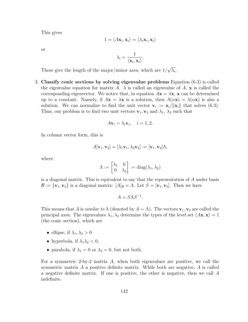
This gives
1 = 〈Axi,xi〉 = 〈λixi,xi〉
or
λi =1
〈xi,xi〉.
These give the length of the major/minor axes, which are 1/√λi.
3. Classify conic sections by solving eigenvalue problems Equation (6.3) is calledthe eigenvalue equation for matrix A. λ is called an eigenvalue of A, x is called thecorresponding eigenvector. We notice that, in equation Ax = λx, x can be determinedup to a constant. Namely, if Ax = λx is a solution, then A(αx) = λ(αx) is also asolution. We can normalize to find the unit vector vi := xi/‖xi‖ that solves (6.3).Thus, our problem is to find two unit vectors v1,v2 and λ1, λ2 such that
Avi = λivi, i = 1, 2.
In column vector form, this is
A[v1,v2] = [λ1v1, λ2v2] := [v1,v2]Λ,
where
Λ :=
[λ1 00 λ2
]:= diag(λ1, λ2)
is a diagonal matrix. This is equivalent to say that the representation of A under basisB := v1,v2 is a diagonal matrix: [A]B = Λ. Let S = [v1,v2]. Then we have
A = SΛS−1.
This means that A is similar to Λ (denoted by A ∼ Λ). The vectors v1,v2 are called theprincipal axes. The eigenvalues λ1, λ2 determine the types of the level set 〈Ax,x〉 = 1(the conic section), which are
• ellipse, if λ1, λ2 > 0
• hyperbola, if λ1λ2 < 0,
• parabola, if λ1 = 0 or λ2 = 0, but not both.
For a symmetric 2-by-2 matrix A, when both eigenvalues are positive, we call thesymmetric matrix A a positive definite matrix. While both are negative, A is calleda negative definite matrix. If one is positive, the other is negative, then we call Aindefinite.
142

6.1.2 Procedure to solve an eigenvalue problem
The goal of this subsection is to solve an eigenvalue problem in details. Let
A =
[a bb c
].
be a real-valued 2× 2 symmetric matrix.
1. Finding eigenvalues Definition: A pair (λ,v) is called an eigen pair of A if v 6= 0and
Av = λv.
This is equivalent to N(A− λI) 6= 0 ⇔ det(λI − A) = 0. Thus, our first step is tosolve the following characteristic equation for eigenvalues λ:
pA(λ) := det(λI − A) = 0.
For the present 2× 2 case, this is∣∣∣∣λ− a −b−b λ− c
∣∣∣∣ = 0.
It givesλ2 − Tλ+D = 0,
whereT = a+ c, D = ac− b2.
They are called the trace and the determinant of matrix A, respectively. The solutionsof this quadratic equation are
λ1 =T −√T 2 − 4D
2, λ2 =
T +√T 2 − 4D
2.
Note thatT 2 − 4D = (a+ c)2 − 4(ac− b2) = (a− c)2 + 4b2 ≥ 0.
Thus, the eigenvalues are real.
2. Find the corresponding eigenvectors vi. We solve the equation
(A− λi)vi = 0.
For λ1, this equation is [λ1 − a −b−b λ1 − c
] [x1
x2
]=
[00
].
It gives
v1 =
[b
λ1 − a
].
143
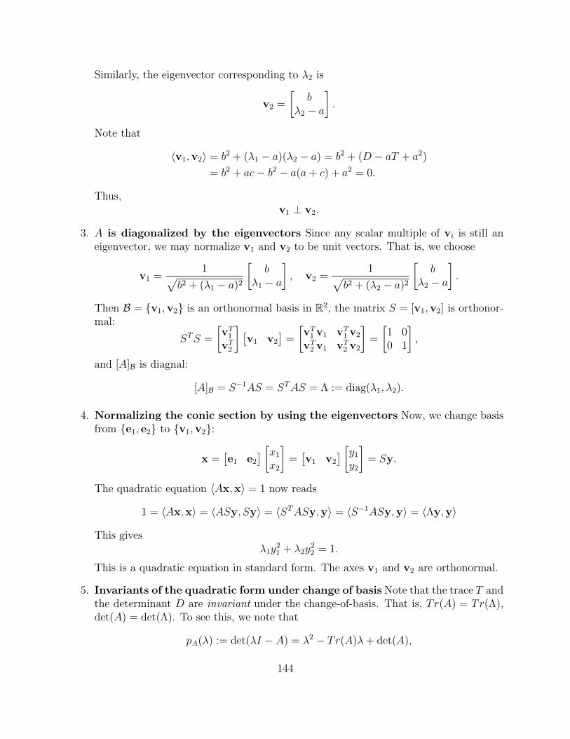
Similarly, the eigenvector corresponding to λ2 is
v2 =
[b
λ2 − a
].
Note that
〈v1,v2〉 = b2 + (λ1 − a)(λ2 − a) = b2 + (D − aT + a2)
= b2 + ac− b2 − a(a+ c) + a2 = 0.
Thus,v1 ⊥ v2.
3. A is diagonalized by the eigenvectors Since any scalar multiple of vi is still aneigenvector, we may normalize v1 and v2 to be unit vectors. That is, we choose
v1 =1√
b2 + (λ1 − a)2
[b
λ1 − a
], v2 =
1√b2 + (λ2 − a)2
[b
λ2 − a
].
Then B = v1,v2 is an orthonormal basis in R2, the matrix S = [v1,v2] is orthonor-mal:
STS =
[vT1vT2
] [v1 v2
]=
[vT1 v1 vT1 v2
vT2 v1 vT2 v2
]=
[1 00 1
],
and [A]B is diagnal:
[A]B = S−1AS = STAS = Λ := diag(λ1, λ2).
4. Normalizing the conic section by using the eigenvectors Now, we change basisfrom e1, e2 to v1,v2:
x =[e1 e2
] [x1
x2
]=[v1 v2
] [y1
y2
]= Sy.
The quadratic equation 〈Ax,x〉 = 1 now reads
1 = 〈Ax,x〉 = 〈ASy, Sy〉 = 〈STASy,y〉 = 〈S−1ASy,y〉 = 〈Λy,y〉
This givesλ1y
21 + λ2y
22 = 1.
This is a quadratic equation in standard form. The axes v1 and v2 are orthonormal.
5. Invariants of the quadratic form under change of basis Note that the trace T andthe determinant D are invariant under the change-of-basis. That is, Tr(A) = Tr(Λ),det(A) = det(Λ). To see this, we note that
pA(λ) := det(λI − A) = λ2 − Tr(A)λ+ det(A),
144

whilepΛ(λ) := det(λI − Λ) = λ2 − Tr(Λ)λ+ det(Λ).
But, from A = SΛS−1, we get
det(λI − A) = det(λI − SΛS−1) = det(S(λI − Λ)S−1)
= det(S) det(λI − Λ) det(S−1) = det(λI − Λ).
Thus, the coefficients of the two polynomials are identical. It means that they areinvariant under change of basis.
6. Example: Let
A =1
5
[13 −4−4 7
]The eigenvalues λi are solutions of the characteristic equation
det(λI − A) =
∣∣∣∣135− λ −4
5
−45
75− λ
∣∣∣∣ = 0.
This isλ2 − 4λ+ 3 = 0.
Its solutions areλ1 = 1, λ2 = 3.
The eigenvector corresponding to λ1 satisfies
(A− I)v1 = 0
which is [135− 1 −4
5
−45
75− 1
] [x1
x2
]=
[00
].
This gives
v1 =1√5
[12
]Similarly, the eigenvector v2 satisfies
(A− 3I)v2 = 0
which is [135− 3 −4
5
−45
75− 3
] [x1
x2
]=
[00
].
This gives
v2 =1√5
[−21
]145

The new equation under the change of basis:[x1
x2
]=[v1 v2
] [y1
y2
]is
y21 + 3y2
2 = 1.
This is an ellipse with axes lengths 1 and 1/√
3. The major axis is v1. The minor axisis v2.
Exercise 6.1. 1. (Strang pp. 328) Find the eigenvalues/eigenvectors of the followingmatrices
(a)
[1 33 5
], (b)
[1 −1−1 1
], (c)
[−1 22 −8
].
6.2 Eigen expansion for 2-by-2 matrices
1. Goal Let us study eigenvalue problem for general 2-by-2 real-valued matrix A. Theyappear in ODE problems, and many problems in stochastic process. The goal there isto compute Ak and exp(tA).
2. Finding eigenvalues and eigenvectors Let
A =
[a bc d
], a, b, c, d ∈ R. (6.4)
An eigenvalue λ of A satisfies
det(λI − A) =
∣∣∣∣λ− a −b−c λ− d
∣∣∣∣ = 0,
orλ2 − Tλ+D = 0,
whereT = a+ d, D = ad− bc
are the trace and determinant of A, respectively. The roots are
λ1 =T −√T 2 − 4D
2, λ2 =
T +√T 2 − 4D
2. (6.5)
The corresponding eigenvectors are
v1 =
[b
λ1 − a
], v2 =
[b
λ2 − a
].
146

3. Three cases:
(1) λ1, λ2 are real and distinct,
(2) λ1 = λ2 are real,
(3) λ1, λ2 are complex conjugates.
6.2.1 Diagonalizable case: λ1, λ2 are real and distinct
In this case, the corresponding eigenvectors v1,v2 are also real.
1. v1,v2 is independent in R2. Suppose there are c1, c2 such that
c1v1 + c2v2 = 0.
Applying A to this equation, using Avi = λivi, we get
c1λ1v1 + c2λ2v2 = 0.
Eliminating c1 from these two equations, we get
c2(λ2 − λ1)v2 = 0.
The condition λ1 6= λ2 implies c2 = 0. From this we also get c1 = 0.
2. Matrix A is diagonalized by the basis v1,v2 in R2. Let S = [v1,v2]. The formulaAvi = λivi, i = 1, 2 can be casted as
A[v1,v2] = [v1,v2]Λ, Λ = diag(λ1, λ2),
orA = SΛS−1.
3. With this eigen expansion, we can compute Ak, exp(tA) as the follows.
Ak = (SΛS−1)k = (SΛS−1)(SΛS−1) · · · (SΛS−1) = SΛkS−1.
Λk =
[λ1 00 λ2
]· · ·[λ1 00 λ2
]=
[λk1 00 λk2
]
exp(tA) =∞∑k=0
1
k!(tA)k =
∞∑k=0
tk
k!(SΛS−1)k
= S
(∞∑k=0
tk
k!Λk
)S−1 = S
[etλ1 00 etλ2
]S−1.
147

6.2.2 Double root and Jordan form
In this case, λ1 = λ2. This is a double root.
1. Let us study this case from special examples. Consider the following two matrices
A =
[λ 10 λ
], Λ =
[λ 00 λ
]You can check that they are not similar to each other. (If yes, then there exists S suchthat AS = SΛ. Show that no such a matrix can exist.)
The above example shows that A cannot be diagonalized. Yet, it is not hard to computeAn and exp(tA). Let us compute them below.
A2 =
[λ 10 λ
] [λ 10 λ
]=
[λ2 2λ0 λ2
],
A3 =
[λ2 2λ0 λ2
] [λ 10 λ
]=
[λ3 3λ2
0 λ3
].
In general, we have
An =
[λn nλn−1
0 λn
].
You can check this formula by mathematical induction. We can also see anothercalculation. We write
A = λI +N, N =
[0 10 0
].
The matrix N is called a nilpotent matrix. It satisfies N2 = 0. We have
An = (λI +N)n = λnI + nλn−1IN =
[λn nλn−1
0 λn
].
Note that the matrix multiplication does not have commutativity. But here, the matrixinvolved is the identity matrix I, which commutes with any matrix. To compute theexponential function of A, we use Taylor expansion
exp(tA) =∞∑n=0
1
n!(tA)n =
∞∑n=0
tn
n!
[λn nλn−1
0 λn
]=
[etλ tetλ
0 etλ
].
We call such matrix A is a Jordan form. Our next question is: Can a general matrixwith double eigenvalue be transformed to a Jordan form? The answer is Yes! Seebelow.
148

2. Let us consider general A (6.4) with double eigenvalues (6.5): λ1 = λ2 = λ. SinceA− λI is singular, its rank can only be 1 or 0. If the rank is 0, then A = λI. This isa trivial case. If the rank is 1, then there is only one eigenvector v1(up to scaling):
(A− λI)v1 = 0.
Now, we consider the equation
(A− λI)v2 = v1
This will give us[Av1, Av2] = [λv1,v1 + λv2],
or
A[v1,v2] = [v1,v2]
[λ 10 λ
].
Thus, we only need to solve the (A− λI)v2 = v1. The trick is the follows. We pick upany vector in R2 to be v2 such that (A−λI)v2 6= 0. Then we redefine v1 as (A−λI)v2.We need to show that (A− λI)v1 = 0. This is equivalent to
(A− λI)2v2 = 0.
This indeed holds for any vector v ∈ R2. This is the amazing Caley-Hamilton theorem,
which will discuss this later. For the moment, let us check it: The matrix A =
[a bc d
]satisfies
A2 − (a+ d)A+ (ad− bc)I = 0.
(check this by yourself.) So, we can find v1,v2 which convert A to Jordan form.
3. Let us find a Jordan form for a concrete matrix.
A =
[5 −11 3
]The eigenvalue λ satisfies ∣∣∣∣λ− 5 1
−1 λ− 3
∣∣∣∣ = 0.
This givesλ2 − 8λ+ 16 = 0.
The eigenvalue is 4 with multiplicity 2. Let us choose v2 = [1, 0]T . Then define
v1 = (A− 4I)v2 =
[1 −11 −1
] [10
]=
[11
]Thus, A becomes a Jordan form under the similarity transform AS = SJ , where
[v1,v2] =
[1 11 0
], J =
[4 10 4
].
You may wonder what happens if we choose a different v2. Try it by yourself.
149

6.2.3 λ1, λ2 are complex conjugates
When T − 4D < 0, we don’t have real eigenvalues and no real-valued eigenvectors. If weextend our space from R2 to C2, we can still find eigenvalues in C and eigenvectors in C2.It turns out such extension is useful for applications. So, let us work out such extension.
1. Let us start from a concrete example. Let
J =
[0 −11 0
].
The eigenvalues are
λ1 = −i, λ2 = i.
If we extend R2 to C2, then the corresponding eigenvectors in C2 are
v1 =
[1i
], v2 =
[1−i
].
They are complex conjugates. The similarity matrix is
S =
[1 1i −i
], S−1 =
1
2
[1 −i1 i
].
The matrix
J = SΛS−1, Λ =
[−i 00 i
].
Then
Jn = (SΛS−1)(SΛS−1) · · · (SΛS−1) = SΛnS−1.
exp(θJ) =∞∑k=0
1
k!(θJ)k =
∞∑k=0
θk
k!(SΛS−1)k = S
(∞∑k=0
θk
k!Λk
)S−1
= S
[e−iθ 0
0 eiθ
]S−1 =
1
2
[1 1i −i
] [e−iθ 0
0 eiθ
] [1 −i1 i
]=
[cos θ − sin θsin θ cos θ
].
2. Let us study the general case. We claim that: If A is real, then the eigenvalues andeigenvectors of A are conjugate pair. That means, the two eigenvalues are λ and λ,the corresponding eigenvectors are v and v. Here, the complex conjugate is defined as
a+ ib := a− ib.
This is simple. If (λ,v) is an eigen pair of A:
Av = λv,
150

thenAv = Av = λv = λv.
Thus, (λ, v) is another eigen pair of A if λ 6= λ. That is, if λ is not real, then λ 6= λand v 6= v. Indeed, v and v are independent. In C2, v, v constitute a basis. LetS = [v, v]. Then
A = SΛS−1, Λ = diag(λ, λ).
The power and exponential functions are given by
An = SΛnS−1 = Sdiag(λn, λn)S−1,
exp(tA) = S exp(tΛ)S−1 = Sdiag(etλ, etλ)S−1. (6.6)
3. Note that the expressions of both An and exp(tA) on the right-hand side are stillreal-valued matrices. In fact, we can translate the eigen expansion: AS = SΛ in realcoefficients. Suppose
λ = α + iβ, v = v1 + iv2, vi ∈ R2.
ThenA[v, v] = [v, v]diag(λ, λ)
can be expressed as
A[v1,v2]
[1 1i −i
]= [v1,v2]
[1 1i −i
] [α + iβ 0
0 α− iβ
]Thus,
A[v1,v2] = [v1,v2]
[1 1i −i
] [α + iβ 0
0 α− iβ
]1
2
[1 −i1 i
]= [v1,v2] (αI + βJ) , J =
[0 −11 0
].
Now, let S = [v1,v2]. You can show that
exp(tA) = Seαt exp(tJ)S−1 = Seαt[cos(tβ) − sin(tβ)sin(tβ) cos(tβ)
]S−1.
Exercise 6.2. 1. Find exp(tA) for the following matrices.
(a)
[1 23 2
], (b)
[1 −13 1
]
151

2. The Nilpotent matrix in Rn has the form
N =
0 1 0 · · · 0
0 1 · · · 0. . . . . .
10
n×n
Find N2, N3 and show Nn = 0.
3. A matrix N is called nilpotent if there exists k > 0 such that Nk = 0. Let us
consider a Nilpotent matrix N =
[a bc d
]in M2. Suppose N2 = 0.
(a) Prove all eigenvalues of N must be zeros.
(b) Find the conditions on a, b, c, d such that N is a Nilpotent matrix.
(c) If c = 0, then a, d = 0.
(d) Find a basis v1,v2 in R2 such that N ∼[0 10 0
]under the basis v1,v2.
6.3 Eigen expansion for symmetric matrices
The goal of this section is to find eigen expansion for symmetric matrix A ∈ Mn(R). Thatis, we look for orthonormal basis v1, ...,vn and λ1, ..., λn ∈ R such that
A[v1, ...,vn] = [v1, ...,vn]diag(λ1, ..., λn).
6.3.1 Eigen expansion for symmetric matrices
1. Definition: eigen pair of A over a field F. Let F be a field, either R or C. LetA ∈ Mn(F) be a F-valued n-by-n matrix. A pair (λ,v) with λ ∈ F and 0 6= v ∈ Fnsatisfying
Av = λv
is called an eigen pair of A over F. We have seen that a real-valued matrix may not
have eigen pair over R, but can have eigen pairs over C. For instance, A =
[0 −11 0
]has no eogenvalue over R, but has complex eigenvalue i and −i. The correspondingeigenvectors are [i, 1]T and [−i, 1]T .
2. Note that λ is an eigenvalue of A if and only if
pA(λ) := det(λI − A) = 0.
152

The polynomial pA(λ) is called the characteristic polynomial of A. The roots of apolynomial are in general complex numbers. Thus, we inevitably encounter complexeigenvalues. We thus extend Rn to Cn.
3. The vector space Cn is an n-dimensional space over C with the standard basis
e1 =
1...0
n×1
, ..., en :=
0...1
n×1
.
A vector v ∈ Cn can be uniquely represented as
v =n∑i=1
viei, with vi ∈ C.
The complex conjugate of a complex number z = a+ ib is defined as z := a− ib. Theconjugate operation satisfies
z1 + z2 = z1 + z2, z1z2 = z1z2.
Further, z is real if and only if z = z. For v =∑n
i=1 viei ∈ Cn, its complex conjugateis defined as
v =n∑i=1
viei.
4. Conjugate pairs of eigenvalue/eigenvector.
Proposition 6.1. If A ∈Mn(R), then the eigenvalues/eigenvectors are pairs of com-plex conjugates. That is, if (λ,v) is an eigen pair of A, so is (λ, v).
5. Inner product structure in Cn: In Cn, we define the inner product 〈·, ·〉 by
〈v,w〉 := vTw =n∑i=1
viwi.
Then
〈v,v〉 =n∑i=1
|vi|2 > 0, for all v 6= 0.
The norm of a complex vector v is defined as ‖v‖ =√〈v,v〉.
6. Let (V, 〈·, ·〉) be a vector space with inner product 〈·, ·〉. An operator T ∈ L(V ) iscalled self-adjoint if
〈Tu,v〉 = 〈u, Tv〉 for all u,v ∈ V.
153

In this definition, we only assume there is an inner product structure in V . The vectorspace V can be over R or C. Suppose A is a matrix representation of T ∈ L(V ). Thenthe condition for self-adjointness of T is
AT = A, if V is over R
AT = A, if V is over C.
See Proposition below for the part of the proof. You may fill out the rest of the proof.
Proposition 6.2. Let A ∈Mn(C). Then A is self-adjoint in (Cn, 〈·, ·〉) if and only ifAT = A.
Proof. On one-hand, we have
〈Au,v〉 =∑i
(∑j
aijuj)vi =∑i
∑j
aijujvi;
On the other hand,
〈u, Av〉 =∑i
ui∑j
aijvj =∑j
∑i
ujajivi.
In the above formula, the second equality comes from switching indices i and j. Fromself-adjointness of A, the above two formulae equal for all u,v ∈ Cn. This is equivalentto aij = aji.
7. The eigenvalues of self-adjoint operators must be real.
Proposition 6.3. The eigenvalues of self-adjoint operators are real.
Proof. If (λ,v) is an eigen pair of A over C. Then
λ〈v,v〉 = 〈λv,v〉 = 〈Av,v〉 = 〈v, Av〉 = 〈v, λv〉 = λ〈v,v〉.
Since v is an eigenvector, v 6= 0. Thus we get λ = λ.
In the example above, A =
[0 1−1 0
], the eigenvalues are i and −i. For A =
[a bc d
],
the eigenvalues are
λ =1
2T ±√T 2 − 4D
where T = a+ d, D = ad− bc. The discriminant
T 2 − 4D = (a− d)2 + 4bc.
We see that if b = c (i.e. A is symmetric) then the eigenvalues are real.
154

8. When A ∈Mn(R) and the eigenvalue λ is real, then
det(λI − A) = 0⇔ N(λI − A) 6= 0.
Thus, there exists v ∈ Rn such that
Av = λv.
We conclude that: if λ is a real-valued eigenvalue of A, then there must have a corre-sponding eigenvector v ∈ Rn. Let us denote
E(λ) := N(λI − A) ⊂ Rn,
called the eigenspace of A corresponding to λ.
Proposition 6.4. If λ and µ are two distinct eigenvalues of A, then the two eigenspacesE(λ) and E(µ) are perpendicular in Rn.
Proof. Suppose u ∈ E(λ) and v ∈ E(µ).
λ〈u,v〉 = 〈λu,v〉 = 〈Au,v〉 = 〈u, Av〉 = 〈u, µv〉 = µ〈u,v〉.
The second equality is due to λ ∈ R. The fourth equality is from A being self-adjoint.Since λ 6= µ, we get 〈u,v〉 = 0.
9. Suppose A ∈ L(V ). A subspace U ⊂ V is called invariant under A if AU ⊂ U .
Proposition 6.5. Suppose A ∈ Mn(R) is self-adjoint. Suppose U ⊂ V is invariantunder A. Then U⊥ is also invariant under A, and A|U⊥ is also self-adjoint.
Proof. (a) Suppose v ∈ U⊥. This means that 〈v,u〉 = 0 for all u ∈ U . Then
〈Av,u〉 = 〈v, Au〉 = 0,
because Au ∈ U . Thus, Av ∈ U⊥. This shows AU⊥ ⊂ U⊥.
(b) The restriction operator A|U⊥ is defined to be
A|U⊥(v) := Av for v ∈ U⊥.
Thus, for any v1,v2 ∈ U⊥,
〈A|U⊥v1,v2〉 = 〈Av1,v2〉 = 〈v1, Av2〉 = 〈v1, A|U⊥v2〉.
Thus, A|U⊥ is self-adjoint in L(U⊥).
155

Theorem 6.1. Suppose A ∈ L(V ) is self-adjoint. Then there exists an orthonor-mal basis B = v1, ...,vn in V and real numbers λ1, ..., λn such that
Avi = λvi, i = 1, ..., n.
Proof. (a) We prove this theorem by mathematical induction in dimV .
(b) If dimV = 1, then A is a scalar multiplication: Av = av. The theorem is triviallytrue.
(c) Suppose the theorem is true for all V with dimV < n. Now, suppose A ∈ L(V )with dimV = n. We claim that A has at least one eigenvalue. This is becausethe characteristic polynomial pA(λ) := det(A−λI) has at least one root in C (bythe fundamental theorem of algebra). Then by Proposition 6.3, such eigenvaluemust be real. Thus, there exists λ ∈ R such that
det(λI − A) = 0⇔ N(λI − A) = E(λ) 6= 0.
(d) Let U = E(λ). By Proposition 6.5, A|U⊥ ∈ L(U⊥) and self-adjoint. NotedimU⊥ < n. By induction, there exists an orthonormal basis B1 = v1, ...,vmfor U⊥ such that
Avi = λivi, i = 1, ...m.
(e) Now V = U ⊕U⊥. We have an orthonormal basis B1 in U⊥. Let us extend B1 toan orthonormal basis in V by picking up an orthonormal basis B′ = vm+1, ...,vnin E(λ). They satisfy
Avi = λvi, i = m+ 1, ..., n.
Then v1, ...,vm, ...,vn is an orthonormal basis of V and they are eigenvectorsof A.
6.4 Singular value decomposition (SVD)
6.4.1 Theory of SVD
Theorem 6.2. Let V , W be real vector spaces with inner products. Suppose dimV = nand dimW = m. Suppose A ∈ L(V,W ) and A 6= 0. Then there exist orthonormal basesv1, ...,vn in V and u1, ...,um in W , and singular values
σ1 ≥ σ2 ≥ · · · ≥ σr > 0
156

such that
A =r∑i=1
σiuivTi . (6.7)
Equivalently, A is decomposed into
A = UΣV T , (6.8)
where
U = [u1, ...,um], V = [v1, ...,vn], Σ =
σ1
. . .
σr
m×n
.
Proof. 1. First we note that ATA ∈ L(V ) is self-adjoint (which is equivalent to symmetricfor real vector spaces).
2. By spectral decomposition theorem, there exists λ1, ..., λn ∈ R and an orthonormalbasis v1, ...,vn such that
ATAvi = λivi, i = 1, ..., n.
3. We claim that the eigenvalues λi ≥ 0. Because
λi = λi〈vi,vi〉 = 〈λivi,vi〉 = 〈ATAvi,vi〉 = 〈Avi, Avi〉 ≥ 0.
4. Let us order these eigenvalues by
λ1 ≥ λ2 ≥ · · · ≥ λr > 0,
λr+1 = · · · = λn = 0.
5. The subspace N(ATA) = Span(vr+1, ...,vn), and R(ATA) = Span(v1, ...,vr). We haveseen that N(ATA) = N(A) and R(ATA) = R(AT ).
6. For i = 1, ..., r, define
σi :=√λi, ui :=
1
σiAvi.
Then we haveAvi = σiui.
and
〈ui,ui〉 =1
σ2i
〈Avi, Avi〉 =1
σ2i
〈ATAvi,vi〉 =1
σ2i
〈σ2i vi,vi〉 = 1,
σiσj〈ui,uj〉 = 〈σiui, σjuj〉 = 〈Avi, Avj〉 = 〈ATAvi,vj〉 = 〈λivi,vj〉 = 0.
Thus, u1, ...,ur is orthonormal in W . We can extend it to u1, ...,ur,ur+1, ...,umto be an orthonormal basis of W .
157

7. For any v ∈ V ,
v =n∑i=1
〈v,vi〉vi
and
Av = A
(n∑i=1
〈v,vi〉vi
)=
r∑i=1
σi〈v,vi〉ui.
This shows R(A) = Span(u1, ...,ur) and
A =r∑i=1
σiuivTi .
From four subspace theorem, we get N(AT ) = R(A)⊥ = Span(ur+1, ...,um).
Example Let us work out an example by assigning U , Σ and V first. We construct A fromA = UΣV T . We choose
U =1√2
[1 11 −1
], Σ =
[2 0 00 1 0
], V T =
1√2
1 0 −11 0 10 1 0
.The matrix
A = UΣV T =1
2
[3 0 −11 0 −3
].
ATA =1
4
10 0 −60 0 0−6 0 10
, AAT =1
4
[10 66 10
].
You can check that the eigenvalues of AAT are λ1 = 4, λ2 = 1 with eigenvectors
u1 =1
2
[11
], u2 =
1
2
[1−1
].
The eigenvalues of ATA are λ1 = 4, λ2 = 1, λ3 = 0. The corresponding eigenvectors are
v1 =1√2
[1 0 −1
], v2 =
1√2
[1 0 1
], v3 =
[0 1 0
].
The SVD isA =
√λ1u1v
T1 +
√λ2u2v
T2
1
2
[3 0 −11 0 −3
]= 2
1
2
[1 0 −11 0 −1
]+
1
2
[1 0 1−1 0 −1
].
158

Exercise 6.3. 1. Find the SVD for the matrix A =
[3 40 5
].
2. (Strang) Find SVD for the matrix
A =
0 2 00 0 30 0 0
.3. Let A ∈Mn(R). Do ATA and AAT have the same eigenvalues?
4. If R ∈Mn(R) is a rotation, what is the SVD of R?
5. Suppose PU is an orthogonal projection onto a subspace U ⊂ V ,what is the SVDof PU?
6. Suppose A = UΣV T is invertible. What is the SVD of A−1?
6.4.2 SVD and the four fundamental subspaces
The four fundamental subspaces theorem is refined by the singular value decompositiontheorem.
Theorem 6.3. Let V,W be inner product spaces with dimensions n and m. Let A ∈L(V,W ). Then we can find an orthonormal basis v1, ...,vn in V with
R(AT ) = Span(v1, ...,vr), N(A) = Span(vr+1, ...,vn),
and an orthonormal basis u1, ...,um in W with
R(A) = Span(u1, ...,ur), N(AT ) = Span(ur+1, ...,um).
The linear map A : R(AT )→ R(A) is a stretching on vi
Avi = σiui, i = 1, ..., r.
6.4.3 SVD and the least-squares method
Corollary 6.1. Given b ∈ W . The least square solution x∗ ∈ R(AT ) for
‖Ax∗ − b‖2 = minz‖Az− b‖2
159

is given by
x∗ =r∑i=1
1
σi〈b,ui〉vi. (6.9)
Remark This solution is usually denoted by x∗ = A+b, the pseudo inverse of A. It satisfies
A+A = PR(AT ), AA+ = PR(A).
where PR(AT ) is the orthogonal projection onto the subspace R(AT ) in V , and PR(A) is theorthogonal projection onto the subspace R(A) in W .
6.4.4 SVD and deformation in continuum mechanics
In continuum mechanics, the flow is described by the flow map x(t,X), where X ∈ R3 calledthe material coordinate, x ∈ R3, called the observer’s coordinate. The deformation gradientF (t,X) is defined as
F iα(t,X) :=
∂xi
∂Xα(t,X), i = 1, 2, 3, α = 1, 2, 3.
The SVD of F characterizes the deformation of the flow:
• F is decomposed into F = UΣV T .
• In the material frame of reference (the space V ), choose an orthonormal basis v1,v2,v3,then F is a stretching on each axis by σi. A unit sphere is stretched to an ellipsoidwith axes lengths σ1, σ2, σ3.
• The material also undergoes a rotation U in the observer’s coordinate. The resultingdeformation is UΣV T .
• The longest stretching ratio is
σ1 = maxdX∈R3
‖FdX‖‖dX‖
= maxdX∈R3
√〈FdX,FdX〉√〈dX, dX〉
= maxdX∈R3
√〈F TFdX, dX〉√〈dX, dX〉
.
Here, dX an infinitesimal tangent vector in the material domain. Its image dx =FdX is the infinitesimal tangent vector in the observer’s domain. Thus, ‖dx‖/‖dX‖measures the stretching ratio after deformation.
SVD and polar decomposition of matrices A polar representation of a complex is
z = reiθ
160

That is, z is factorized into a stretching and a rotation. Similarly, we want to factorizea matrix A ∈ L(Rn) into a stretching and a rotation. The stretching is indeed a positivedefinite matrix. We have
A = SlR := (UΣUT )(UV T ),
A = RSr := (UV T )(V ΣV T ).
Here, R is a rotation. Sl, Sr are symmetric. Their eigenvalues are σi > 0, i = 1, ..., r. If A isnon-singular, then all σi are positive and Sl and Sr are positive definite.
6.4.5 SVD and the discrete Laplacian
We consider the (minus) discrete Laplacian with three kinds of boundary condition:
• Dirichlet boundary condition
• Neumann boundary condition
• Periodic boundary condition.
1. Dirichlet Laplacian. Consider functions defined on the nodes: xj = j/n, j = 0, ..., nwith zero boundary. That is
u : x0, x,..., xn → R with u(x0) = u(xn) = 0.
These discrete functions form a vector space.
V := u = (u(x0), ..., u(xn))|u(x0) = u(xn) = 0.
We abbreviate u(xj) by uj. Next, we consider another set of functions which are definedon edges ei := (xi−1, xi), i = 1, ..., n. That is,
v : e1, ..., en → R.
These discrete functions also form a vector space:
W := v = (v1, ..., vn)|vi ∈ R.
Here, we abbreviate v(ei) by vi. Note that dimV = n− 1, dimW = n.
Define the difference operator
D : V → W, Du(ei) = u(xi)− u(xi−1).
In terms of the abbreviated notation,
(Du)i = ui − ui−1, i = 1, ..., n.
161

The matrix representation of D under standard basis is
D =
1 0 0 · · · 0−1 1 0 · · · 00 −1 1 · · · 0
. . . . . .
−1 10 0 · · · 0 −1
n×(n−1)
DT =
1 −1 0 · · · 0 00 1 −1 · · · 0 0
0 0 1. . .
......
. . . . . . −1 00 0 · · · 0 1 −1
(n−1)×n
The Laplacian with Dirichlet boundary condition is defined to be
LD := DTD =
2 −1 0 · · · 0−1 2 −1 · · · 0
. . . . . . . . .
−1 2 −10 −1 2
(n−1)×(n−1)
.
2. Neumann Laplacian The Neumann Laplacian is LN = DDT :
LN :=
1 −1 0 · · · 0−1 2 −1 · · · 0
. . . . . . . . .
−1 2 −10 −1 1
n×n
3. Periodic Laplacian The underlying nodes and edges are required to satisfy xn = x0
and en = e0. The functions defined on nodes are
V := u = (u0, ..., un)|u0 = un, uj ∈ R
The functions defined on edges are
W := v = (v1, ..., vn)|v0 = vn, vi ∈ R.
162

The difference operator DP : V → W is
DP =
1 0 0 · · · −1−1 1 0 · · · 00 −1 1 · · · 0
. . . . . .
−1 11 0 · · · 0 −1
n×n
The corresponding Laplacian with periodic boundary condition becomes
LP := DTPDP =
2 −1 0 · · · −1−1 2 −1 · · · 0
. . . . . . . . .
−1 2 −1−1 −1 2
n×n
4. We consider the following vectors
vk =
sin(kπ/n)sin(2kπ/n)
...sin(2kπ(n− 1)/n)
∈ Rn−1, k = 1, ..., n− 1,
uk =
cos(kπ/n)cos(2kπ/n)
...cos(2kπ(n− 1)/n)
∈ Rn, k = 0, ..., n− 1,
wk =
1
e2πik/n
...e2πik(n−1)/n
∈ Cn, k = 0, 1, ..., n− 1.
Exercise 6.4. 1. Show that vk, k = 1, ..., n − 1 are eigenvectors of LD. Find thecorresponding eigenvalues.
2. Show that uk, k = 0, ..., n − 1 are eigenvectors of LN . Find the correspondingeigenvalues.
3. Find the SVD of D : Vn−1 → Wn.
163

4. Show that wk, k = 0, ..., n − 1 are eigenvectors of LP . Find the correspondingeigenvalues.
Given a graph G = (V,E). Let D be its incident matrix. D is an |E|× |V | matrix. DTDis a |V | × |V | matrix, which is self-adjoint. It is called the graph Laplacian, which reflectstopological information of the graph.
6.4.6 SVD and principal component analysis (PCA)
6.5 Quadratic Forms
164

Chapter 7
Operators over Complex VectorSpaces
General operator is to find suitable basis, or suitable transformation, that can change theoperator under consideration to a simple form. The simple forms are:
• diagonal form,
• block Jordan form,
• block cyclic form,
• block upper triangular form,
• block tri-diagonal form,
The transformation or the bases we use may be
• Similarity transform: S−1AS,
• Orthonormal transform: S−1AS with STS = I.
• Unitary transform: U−1AU with UTU = I.
In matrix analysis, a general theory allows nonlinear transformation, which can give bestsparse matrix, or low rank matrix.
The spectral theory includes
• If A has full rank of eigenvectors, then A is similar to a diagonal matrix.
• A is normal if and only if A is unitary similar to a diagonal matrix.
• A self-adjoint operator is a normal operator.
• Every matrix is unitary similar to an upper triangular matrix.
• Every matrix is similar to a block Jordan matrix.
165

7.1 Complex number system and Polynomials
7.1.1 Complex number system
We have seen the Euclidean vector space Rn, which is a vector space over the scalar field R.The complex field C is another important field that we will encounter in many branches ofscience and engineering.
1. The complex field is defined as
C := a+ bi | a, b ∈ R,
where i is a formal symbol. It is required to satisfy
i2 = −1.
The addition and multiplication of complex numbers are defined as
(a+ bi) + (c+ di) := (a+ c) + i(b+ d)
(a+ bi)(c+ di) := (ac− bd) + (ad+ bc)i.
The requirement of i2 = −1 is inherited in the multiplication rule. One can check thatC endowed with the addition and multiplication is a field (see the definition in Chapterfor the real number system). In particular, for z = a+ bi 6= 0, we look for c+ di suchthat
(a+ bi)(c+ di) = 1.
This gives
c =a
a2 + b2, d = − b
a2 + b2.
We denote this inverse (of z) by
z−1 =a− bia2 + b2
.
2. Geometrically, C can be viewed as R2, called the complex plane, or the Gauss plane.From geometric viewpoint, the multiplication of a complex number z = a + bi by i isa rotation of z by 90. Thus, the abscissa is the real axis. Its 90 rotation, the verticalaxis, is called the imaginary axis. For a complex number z = a+ bi, we call a the realpart, b the imaginary part. Denote them by
a = Re(z), b = Im(z).
It is natural to define the length of a complex number to be
|a+ bi| :=√a2 + b2,
because 1 and i are perpendicular to each other. It satisfies the usual properties ofnorm: the triangle inequality: |z + w| ≤ |z|+ |w|. In addition, |zw| = |z| |w|.
166

3. It is convenient to introduce the complex conjugate for z = a+ bi as
z = a− bi.With this notation, we have
z1 + z2 = z1 + z2, z1z2 = z1z2.
zz = |z|2, z−1 =z
|z|2, |z| = |z|,
z + z = 2Re(z), z − z = 2Im(z).
A complex number z is real if and only if z = z.
7.1.2 Polynomials
1. Roots of polynomials. The most fundamental property of C is that every polynomialover C has at least a root in C. Unlike C, the real number system R does not havethis property. For example, x2 + 1 = 0 has no root in R. This property is called thefundamental theorem of algebra.
Theorem 7.1 (Fundamental Theorem of Algebra). Every non-constant polynomialover C has a root in C.
Sketch proof. If a polynomial p(z) has no root, then 1/p(z) is bounded and analytic.By Liouville theorem , a bounded analytic function on entire C must be a constant.This contradicts to our assumption.
Proposition 7.1. That λ is a root of p(z) = 0 if and only if there exists a polynomialq(z) with deg(q) = deg(p)− 1 such that
p(z) = (z − λ)q(z).
Corollary 7.1. A polynomial p(z) of degree n can be factorized uniquely as
p(z) = c(z − λ1) · · · (z − λn).
where c 6= 0, λ1, ..., λn ∈ C.
Corollary 7.2. If the coefficients of polynomial p(z) are real, then the roots are inpair, namely, if λ is a root, so is λ.
If we denote such root λ = a+ bi, then the factors
(x− λ)(x− λ) = (x− a)2 + b2.
Corollary 7.3. A real-coefficient polynomial p(x) of degree n can be factorized uniquelyas
p(x) = c(x− λ1) · · · (x− λr)[(x− a1)2 + b21] · · · [(x− as)2 + b2
s]
where, c, λi, aj, bj ∈ R, and r + 2s = n.
2. Great common divisors
3. Lagrange interpolation and partition of unity
167

7.1.3 Complex vector space Cn
1. Cn is the Cartesian product of C:
Cn = a = (a1, ..., an)|ai ∈ C, i = 1, ..., n.
2. In Cn, we define the inner product 〈·, ·〉 as
〈a,b〉 :=n∑i=1
aibi. (7.1)
The inner product has the following properties:
(a) 〈a,b〉 is linear in b,
(b) 〈b, a〉 = 〈a,b〉,(c) 〈a, a〉 ≥ 0,
(d) 〈a, a〉 = 0 if and only if a = 0.
Note that we have
〈a1 + a2,b〉 = 〈a1,b〉+ 〈a2,b〉, 〈λa,b〉 = λ〈a,b〉.
3. We define the norm ‖a‖ :=√〈a, a〉.
4. The above inner product implies the Cauchy-Schwarz inequality:
|〈a,b〉| ≤ ‖a‖‖b‖.
Proof. Consider the quadratic form
0 ≤ ‖ta + b‖2 = 〈ta + b, a + tb〉 = t2‖a‖2 + 2Re〈a,b〉+ ‖b‖2.
Since this quadratic function in t is nonnegative, its discriminant satisfies
|Re〈a,b〉| ≤ ‖a‖‖b‖.
Replacing a by ia, we get
|Re〈ia,b〉| ≤ ‖ia‖‖b‖ = ‖a‖‖b‖.
But |Re〈ia,b〉| = |Im〈a,b〉|, we thus obtain
|〈a,b〉|2 = |Re〈a,b〉|2 + |Im〈a,b〉|2 ≤ ‖a‖2‖b‖2.
168

5. As a consequence of the Cauchy-Schwarz inequality, we have the triangle inequality
‖a + b‖ ≤ ‖a‖+ ‖b‖.
6. The parallelogram law
‖a + b‖2 + ‖a− b‖2 = 2(‖a‖2 + ‖b‖2
).
The geometric reason why this equality is important is that if a norm satisfying theparallelogram law, then you can define an inner product which is compatible to thisnorm.
7. Orthogonality in Cn.
(a) We say that a and b are orthogonal to each other if 〈a,b〉 = 0. We denote thisrelation by a ⊥ b.
(b) The projection of b onto a is defined to be
b‖ :=〈b, a〉‖a‖2
a.
We have
〈b− b‖, a〉 = 〈b, a〉 − 〈b, a〉‖a‖2
〈a, a〉 = 0.
We define the perpendicular part b⊥ := b−b‖. Thus, the vector b is decomposedinto
b = b‖ + b⊥ with b‖ ⊥ b⊥.
(c) Remark.
• There is a difficulty to define the angle between two complex vectors a andb. The main reason is that the inner product 〈a,b〉 is a complex number. Onone hand, if we want the cosine law hold, that is
‖a− b‖2 = ‖a‖2 + ‖b‖2 − 2‖a‖‖b‖ cos θ.
then, by expanding the left-hand side, we should define
cos θ = Re〈a,b〉.
However, the orthogonality from this definition (i.e. Re〈a,b〉 = 0) is differentfrom the orthogonality 〈a,b〉 = 0, which is not correct. On the other hand,from the Cauchy-Schwarz inequality, we may use
cos θ = |〈a,b〉|.
If so, however, we cannot distinguish between an acute angle and an obtuseangle, when both a and b are only real vectors. This is inconsistent to thedefinition of angle in Rn. Indeed, in the theory of linear algebra, we only needthe concept of orthogonality. We don’t need the concept of angle.
169

• Alternatively, in complex analysis, one can define cosine function for complexangle to resolve the aforementioned difficulty. Yet, we will not discuss suchtopic in this elementary course.
8. Dimension The set e1, ..., en constitutes a basis of Cn, thus dimCn = n. However,Cn can also be thought as a vector space over R. Namely, any vector z ∈ Cn can beexpressed as z = a + bi, where a,b ∈ Rn. Thus, there is a natural correspondencebetween Cn and R2n. The set e1, ..., en, e1i, ..., eni constitutes a basis for Cn astreated as a vector space over R.
7.1.4 Trigonometric polynomials
1. Let Tn(C) be the function space spanned by
S = 1, e±ix, ..., e±inx
An element f ∈ Tn(C) is called a trigonometric polynomial of degree n:
f(x) =n∑
k=−n
ckeikx.
The set S is independent:
ˆ 2π
0
eikxei`x dx =
ˆ 2π
0
e−ikxei`x dx
=
ˆ 2π
0
ei(`−k)x dx
=
2π if k = `0 if k 6= `.
Thus, eikx|k = −n, ..., n are orthogonal set, which implies independence.
7.2 Invariant subspaces for operators over complex vec-
tor spaces
7.2.1 Invariant subspaces
Let V be a vector space over C. Let T ∈ L(V ).
Definition 7.1. A subspace U ⊂ V is called an invariant subspace of T if T (U) ⊂ U .
1. The operator T induces a restriction operator T |U ∈ L(U) which is defined by T |U(u) =Tu for u ∈ U . Because U is invariant under T , we have T |Uu ∈ U for u ∈ U . Thus,T |U ∈ L(U).
170

2. Roughly speaking, the eigen-expansion is to decompose V into U1, ..., Um such thateach Ui is invariant under T . Then we reduce the operator T into many smaller anddecoupled operators T |Ui
.
3. The simplest restriction operator T |U is λIU , where I is the identity map.
4. However, there are linear transformations in R2 which cannot be a scalar multiples ofidentity. For instance, a rotation, or a shearing.
Definition 7.2. A complex number λ is called an eigenvalue of T if there exists a 0 6= v ∈ Vsuch that
Tv = λv.
The vector v is called an eigenvector corresponding to the eigenvalue λ. The kernel E(λ) :=N(T − λI) is called the eigenspace corresponding to the eigenvalue λ.
This definition is also applied to matrices, as we treat them as operators in L(Cn).
Criterion to determine an eigenvalue The following criterion is to determine eigenval-ues of a matrix A and an operator T .
Proposition 7.2. Let A be an n× n matrix. Then λ is an eigenvalue of A if and only if
det(λI − A) = 0.
Proof. λ is an eigenvalue of A ⇔ N(λI −A) 6= 0 ⇔ det(λI −A) = 0. The last statementfollows from Theorem ??.
We recall that the determinant of an operator T is independent of the choice of basis.Thus, the above criterion for matrices is also suitable for operators.
Corollary 7.4. Let T ∈ L(V ). Then λ is an eigenvalue of T if and only if
det(λI − T ) = 0.
Definition 7.3. The polynomial pT (λ) := det(λI−T ) is called the characteristic polynomialof T .
The characteristic polynomial is independent the choice of basis. Namely,
pT (λ) = p[T ]B(λ)
for any basis B of V .
Existence of eigenvalue.
171

Theorem 7.2. Let V be a complex vector space. Suppose T ∈ L(V ). Then T has aneigenvalue λ ∈ C.
Proof. 1. λ is an eigenvalue of T if and only if
pT (λ) := det(λI − T ) = 0.
From the fundamental theorem of algebra, all non-constant polynomial has at least aroot in C. Thus, there exists a λ ∈ C such that det(λI − T ) = 0.
2. Recalldet(λI − T ) = 0⇔ N(λI − T ) 6= 0.
Thus, there exists a vector v ∈ V such that
Tv − λv = 0.
Nested invariant subspaces and upper-triangular matrix representation SupposeT ∈ L(V ). Suppose v1, ...,vn is a basis of V such that
Tvj ∈ Span(v1, ...,vj), for j = 1, ..., n.
Then
• The subspace Uj := Span(v1, ...,vj) is invariant under T ;
• The matrix representation of T under B is an upper-triangular matrix. That is
[T ]B =
∗ ∗ · · · ∗0 ∗ · · · ∗...
. . ....
0 · · · ∗
Theorem 7.3. Let V be a complex vector space and T ∈ L(V ). Then there exists a basisB = v1, ...,vn such that the matrix representation of T under B is an upper triangularmatrix.
Proof. 1. We prove this theorem by induction in the dimension of V . For n = 1, this the-orem is trivially true. Suppose it holds for all complex vector space V with dimensions< n. We show it is also true for V with dimV = n.
172

2. By the previous theorem, T has an eigenvalue λ. Then, let U = R(λI − T ). ThendimU < n and U is also invariant under T . Thus, T |U ∈ L(U). By inductionhypothesis, there exists a basis u1, ...,um in U such that
T |Uuj ∈ Spanu1, ...,uj, for j = 1, ...,m.
3. We extend u1, ...,um to B = u1, ...,um,v1, ...,vn, a basis of V . Then for any k,
Tvk = (T − λI)vk + λvk ∈ Span(u1, ...,um,v1, ...,vk).
For j = 1, ...,m,Tuj = T |Uuj ∈ Span(u1, ...,uj).
Thus, T is an upper-triangular matrix under the basis B.
Remark This theorem tells us that
• Eigenvalues are the diagonals of [T ]B. This gives the invariants of T .
• The structure of the invariant subspaces is in B, or equivalently, Uj are nested:
U1 ⊂ U2 ⊂ · · · ⊂ Un = V.
There are two approaches to give more detail structure of T . One relies on the inner productstructure of V . The other does not. We discuss the latter first.
7.3 Diagonalizable and Jordan forms
7.3.1 Eigenspace and generalized eigenspace
1. Generalized eigenspaces. Let V be a vector space over F and T ∈ L(V ).
Definition 7.4. • The set E(λ, T ) := N(λI − T ) is called the eigenspace of Tcorresponding to λ.
• A vector v ∈ V is called a generalized eigenvector of T if there exists a positiveinteger j such that
(λI − T )jv = 0.
• The set of all such generalized eigenvectors, denoted by G(λ, T ) is called thegeneralized eigenspace corresponding to λ.
Clearly,E(λ, T ) ⊂ G(λ, T ).
173

2. Examples: Consider
A1 =
[3 00 2
], A2 =
[2 30 2
], A3 =
2 0 00 2 30 0 2
• The eigenvalues of A1 are 3 and 2. The corresponding eigenvecrtors are e1 and
e2. Thus,
E(3, A1) = G(3, A1) = Span(e1), E(2, A1) = G(2, A1) = Span(e2).
• The eigenvalue of A2 is 2. To find the corresponding eigenvector, we solve
(A2 − 2I)v = 0
for v. This gives x2 = 0. The corresponding eigenvector is e2. Thus,
E(2, A2) = Span(e2), G(2, A2) = Span(e1, e2).
• The eigenvalue of A3 is 2. To find the eigenvectors, we solve the equations
(A3 − 2I)v = 0.
There are two independent eigenvectors: e1 and e3. We note that (A3 − 2I)e2 =3e3. We apply (A3 − 2I) on both sides and get (A3 − 2I)e2 = 0. Thus, e2 is ageneralized eigenvector. From above discussion, we get
E(2, A3) = Span(e1, e3), G(2, A3) = Span(e1, e3, e2).
7.3.2 Diagonalizable operators
1. Diagonalization. Diagonalization of a matrix A is to decompose A into small blocks.Each block is just an 1× 1 matrix.
Definition 7.5. Let V be an n-dimensional vector space over F. An operator T ∈ L(V )is called diagonalizable in F if there exist eigenvalues λi ∈ F , i = 1, ..., n such that thecorresponding eigenvectors B = v1, ...,vn constitutes a basis of V .
In this case, we have
T [v1, ...,vn] = [v1, ...,vn]Λ, Λ :=
λ1
. . .
λn
,where Λ is a diagonal matrix. It is also denoted by diag(λ1, ..., λn). Or equivalently,
[T ]B = diag(λ1, ..., λn).
We say T is diagonalized by B.
174

2. Distinct eigenvalues correspond to independent eigenvectors.
Proposition 7.3. Let T ∈ L(V ). Suppose λ1, ..., λm are distinct eigenvalues of Tcorresponding eigenvectors v1, ...,vm. Then v1, ...,vm is linearly independent.
Proof. Let us prove it by induction. Suppose v1, ...,vk is independent, but vk+1 ∈Span(v1, ...,vk). Then there exist c1, ..., ck, not all zeros, such that
vk+1 =k∑i=1
civi.
Applying T to this equality, we get
λk+1vk+1 =k∑i=1
ciλivi.
Together this the formula for vk+1, we obtain
0 =k∑i=1
ci(λi − λk+1)vi.
By our induction hypothesis and the assumption (λi 6= λj for i 6= j), we get ci = 0 forall i = 1, ..., k. Thus, vk+1 = 0. This contradicts to vk+1 being an eigenvector.
Corollary 7.5. Let T ∈ L(V ). Suppose dimV = n and suppose T has n distincteigenvalues, then T is diagonalizable.
Proof. From the proposition, v1, ...,vn is a linearly independent set in the n dimen-sional space V . Thus, it is a basis. This shows T is diagonalized by v1, ...,vn.
3. Diagonalization procedure Let A be an n× n matrix. The procedure to diagonalize A(if possible) is the following:
(a) Find eigenvalues by solving the characteristic equation
det(λI − A) = 0.
Suppose λ1, ..., λp are the solutions with multiplicities k1, ..., kp.
(b) For each λi, solve the linear equation (say, by Gaussian elimination)
(A− λi)v = 0.
This gives the vectors which span E(λi).
(c) If dimE(λi, A) = ki, i = 1, ..., p, then A is diagonalizable.
The last statement is a theorem, which will be stated and proved after we learned someexamples.
175

7.3.3 Adjoint operator
Given an operator T ∈ L(V ), its adjoint operator T ∗ is defined as the follows: given y ∈ V ,T ∗y is defined such that
〈T ∗y,x〉 = 〈y, Tx〉
for all x ∈ V . Suppose B = v1, ...,vn be a basis of V . Then
[T ∗]B = [T ]TB .
Proof. Let us express T ∈ L(V ), x,y ∈ V in terms of B as the follows:
x =n∑i=1
xivi, y =n∑i=1
yivi, Tvj =n∑i=1
aijvi.
Then
〈Tx,y〉 =∑i
(∑j
aijxj
)yi =
∑j
∑i
ajixiyj.
〈x, T ∗y〉 =∑i
xi
(∑j
[T ∗]ijyj
)=∑i
xi
(∑j
[T ∗]ijyj
).
From 〈Tx,y〉 = 〈x, T ∗y〉 for all x,y, we get
[T ∗]ij = aji, or equivalently, [T ∗]ij = aji.
176

Chapter 8
Applications
8.1 Interpolation and Approximation
8.1.1 Polynomial interpolation
8.1.2 Spline approximation
8.1.3 Fourier approximation
8.1.4 Wavelet approximation
8.2 Modeling linear systems on graphs
8.3 Geometry and topology
8.4 Image processing and inverse problems
8.5 Statistics and machine learning
8.6 Evolution process and dynamical systems
8.7 Markov process
177