Life Cycle Wage Growth across Countries
53
Life Cycle Wage Growth across Countries David Lagakos University of California, San Diego and National Bureau of Economic Research Benjamin Moll Princeton University and National Bureau of Economic Research Tommaso Porzio University of California, San Diego and Centre for Economic Policy Research Nancy Qian Northwestern University, Centre for Economic Policy Research, National Bureau of Economic Research, and Bureau for Research in Economic Analysis of Development Todd Schoellman Federal Reserve Bank of Minneapolis This paper documents how life cycle wage growth varies across coun- tries. We harmonize repeated cross-sectional surveys from a set of coun- tries of all income levels and then measure how wages rise with poten- tial experience. Our main finding is that experience-wage profiles are on average twice as steep in rich countries as in poor countries. In ad- dition, more educated workers have steeper profiles than the less edu- This version supersedes an earlier version of the paper entitled “Experience Matters: Human Capital and Development Accounting.” We thank four anonymous referees and the editor, Erik Hurst, for numerous helpful comments. For helpful suggestions and crit- icisms we also thank Daron Acemoglu, Mark Aguiar, Paco Buera, Francesco Caselli, Thomas Chaney, Sylvain Chassang, Angus Deaton, Mike Golosov, Fatih Guvenen, Lutz Hendricks, Electronically published March 12, 2018 [ Journal of Political Economy, 2018, vol. 126, no. 2] © 2018 by The University of Chicago. All rights reserved. 0022-3808/2018/12602-0008$10.00 797
Transcript of Life Cycle Wage Growth across Countries
Life Cycle Wage Growth across Countries
David Lagakos
University of California, San Diego and National Bureau of Economic Research
Benjamin Moll
Princeton University and National Bureau of Economic Research
Tommaso Porzio
University of California, San Diego and Centre for Economic Policy Research
Nancy Qian
Northwestern University, Centre for Economic Policy Research, National Bureau of EconomicResearch, and Bureau for Research in Economic Analysis of Development
Todd Schoellman
Federal Reserve Bank of Minneapolis
ThHumthe eicismChan
Electro[ Journa© 2018
This paper documents how life cycle wage growth varies across coun-tries.We harmonize repeated cross-sectional surveys from a set of coun-tries of all income levels and then measure how wages rise with poten-tial experience. Our main finding is that experience-wage profiles areon average twice as steep in rich countries as in poor countries. In ad-dition, more educated workers have steeper profiles than the less edu-
is version supersedes an earlier version of the paper entitled “Experience Matters:an Capital and Development Accounting.” We thank four anonymous referees andditor, Erik Hurst, for numerous helpful comments. For helpful suggestions and crit-s we also thank Daron Acemoglu, Mark Aguiar, Paco Buera, Francesco Caselli, Thomasey, Sylvain Chassang, Angus Deaton, Mike Golosov, Fatih Guvenen, Lutz Hendricks,
nically published March 12, 2018l of Political Economy, 2018, vol. 126, no. 2]by The University of Chicago. All rights reserved. 0022-3808/2018/12602-0008$10.00
797
Ginny Wiehardt
https://www.journals.uchicago.edu/toc/jpe/current
Joe KSam Sipantand FMassaQueband cties DSummDynain St.the Fas sup
798 journal of political economy
cated; this accounts for around one-third of cross-country differencesin aggregate profiles. Our findings are consistent with theories inwhich workers in poor countries accumulate less human capital or facegreater search frictions over the life cycle.
I. Introduction
This paper documents how life cycle wage growth varies across countries.It is well known that wages grow substantially over the life cycle in theUnited States and other advanced economies. However, there is littlecomparable evidence from less developed countries. This is unfortunate,as cross-country differences in life cycle wage growth are key for address-ing questions such as the importance of human capital and labor marketfrictions for explaining cross-country income differences (Burdett 1978;Jovanovic 1984; Klenow andRodriguez-Clare 1997; Bils and Klenow 2000;Caselli 2005; Manuelli and Seshadri 2014).We fill this gap by measuring life cycle wage growth in both low- and
high-income countries. We use representative large-sample householdsurveys from18 countries with individual-level data on educational attain-ment, labor earnings, and the number of hours worked. These data allowus to construct comparable measures of hourly wages and potential ex-perience for all countries in our sample.Our main finding is that wages increase substantially more over the
life cycle in rich countries than in poor countries. We take three alterna-tive approaches to measuring life cycle wage growth. The first and sim-plest approach is to construct cross-sectional experience-wage profilesin which experience is measured as years of potential experience, thatis, years elapsed since finishing school. To do this, we computemeanwagesfor each 5-year experience bin relative to the bin with the least experi-ence. We show that profiles are steeper in rich countries than in poorcountries, with differences that are statistically and economically signifi-cant: wages almost double over the life cycle in rich countries whereas
aboski, Nobu Kiyotaki, Pete Klenow, Jonathan Parker, Richard Rogerson, Paul Romer,chulhofer-Wohl, David Sraer, David Weil, and Fabrizio Zillibotti, plus seminar partic-s at Columbia, Chicago, City University of New York, Einaudi Institute for Economicsinance, European University Institute, Harvard, Laval, London School of Economics,chusetts Institute of Technology, Northwestern, Princeton, Rochester, University ofec at Montreal, University of Southern California, Warwick, and the World Bankonference participants at BREAD, German Research Foundation, Northeast Universi-evelopment Consortium, the NBER Summer Institute Growth Workshop, the NBERer Institute Economic Fluctuations and Growth meeting, the Society for Economic
mics annual meetings, and the Human Capital Conference at Washington UniversityLouis. The views expressed herein are those of the authors and not necessarily those ofederal Reserve Bank of Minneapolis or the Federal Reserve System. Data are providedplementary material online.
life cycle wage growth across countries 799
they increase by only around 50 percent in poor countries. Put differently,wages rise almost twice as much in rich countries as in poor ones.Our second approach follows Mincer (1974), which allows us to con-
trol for years of schooling in the standard way. It also provides a frame-work for addressing the well-known challenge to estimating life cycleprofiles in age (or potential experience), which is that age is collinear withtime and birth cohort (i.e., calendar year and birth year). This means thatone cannot separately identify the effect of age from the effect of time orbirth cohort without further restrictions, a point that has not been ad-dressed in the existing cross-country literature. We begin by followingthe standard approach outlined by Hall (1968) and Deaton (1997). Theyshow that experience or age profiles can be estimated if one assumptionabout the source of aggregate income growth is imposed. We find that iftime effects explain half or more of growth, then wages rise more overthe life cycle in rich countries.However, there are two challenges: one doesnot know in general what fraction of growth is due to time effects, and thisfraction could differ across countries.Our third and preferred approach draws on economic theory to ad-
dress this challenge. We draw on a common prediction of theories of lifecycle wage growth that there should be little or no effect of experienceon wages near the end of the life cycle.1 For example, human capital the-ory predicts that the incentive to invest in human capital formation de-clines at the end of the life cycle, while search and matching theory pre-dicts that the incentive to search for better matches declines similarly. Ourinsight, based on the work ofHeckman, Lochner, andTaber (1998), is thatthis theoretical prediction is sufficient to disentangle experience, time,and cohort effects. Intuitively, if we follow a fixed cohort across multiplecross sections for the last years of their working life, then we rule out bothcohort effects (by construction) and experience effects (by the theoreticalresult above), allowing us to attribute any wage changes to time effects.Once we have recovered the aggregate time effects, it is straightforwardto estimate the experience and cohort effects of workers who are not nearthe end of the life cycle. Applying thismethod, we again find that estimatedexperience-wage profiles are substantially steeper in rich countries than inpoor countries.We also experimentwith variants of this idea inwhichwageprofiles are assumed to decrease at the end of the life cycle, for example,because of human capital depreciation, and find similar results.We provide evidence that our findings are robust to a number of alter-
native measurement assumptions and sample restrictions. While our
1 For example, Rubinstein and Weiss (2006) review the literature on life cycle wagegrowth and explain in detail the three main mechanisms emphasized in this literature (hu-man capital investment, search, and learning), noting that all three have “similar implica-tions with respect to the behavior of mean wages, implying rising and concave wage pro-files” (4).

800 journal of political economy
benchmark results focus on full-time male wage workers, we show thatexperience-wage profiles are steeper in rich countries when we includewomen, part-time workers, and the self-employed. To address concernsthat our findings are driven by mismeasurement of experience, we showthat our results are similar when using an alternative measure of expe-rience based on age- and education-specific employment rates. Further-more, adding plausible amounts of measurement error to the age andeducation variables in rich countries does not cause the profiles of richcountries to look like those of poor ones. Finally, we show that our cross-sectional experience profiles from the United States andMexico are sim-ilar to those computed using panel data.We next explore one natural hypothesis for why experience-wage pro-
files are steeper in richer countries, which is that richer countries have agreater fraction of educated workers. While Mincer (1974) found thatUS experience-wage profiles were similar for different education groups,more recent work has tended to find that more educated workers havesteeper experience-wage profiles (Lemieux 2006). Overall, we find thatacross our 18 countries, more educated workers have steeper experience-wage profiles on average than less educated workers and that cross-countrydifferences in the distribution of educational attainment account foraroundone-thirdof theflatter aggregate experienceprofiles inpoor coun-tries. This implies that education is likely to be an important factor forexplaining cross-country differences in life cycle wage growth but alsosuggests that other factors play important roles.We conclude by returning to the interpretation and broader implica-
tions of our findings. Three popular theories of life cycle earnings patternsand wage dynamics are human capital accumulation, on-the-job search,and long-term contracts. While it is hard to provide definitive conclusionsabout which theory best explains our findings, several pieces of evidencepoint to human capital and search frictions as playing important roles.First, when we look at profiles by broad occupation category, we find ro-bust evidence that manual occupations have flatter profiles than cogni-tive occupations. Since manual occupations likely have less scope for life-time learning and since around half of workers in poor countries are inmanual occupations, this suggests a human capital interpretation. Sec-ond, we find that wage variances generally increase over the life cycle,with some evidence of a dip for early experience levels in rich countries.We note that this is predicted by several classes of theories of human cap-ital and search andmatching frictions. Finally, we look at wage profiles forday laborers, who are not engaged in long-term wage contracts, and findthat, in the poor countries for which we have data, these are again flatterthan in rich countries.Both human capital and search theories suggest that our findings may
help explain cross-country income differences. Through the lens of hu-
life cycle wage growth across countries 801
man capital theory, our findings point to a much greater role for humancapital in accounting for cross-country income differences than suggestedby previous studies, in particular those of Klenow and Rodriguez-Clare(1997), Bils and Klenow (2000), and Caselli (2005). Specifically, our find-ings are consistent with workers in rich countries accumulating more hu-man capital over the life cycle than workers in poor countries. This is ex-actly the theoretical prediction of Manuelli and Seshadri (2014). Throughthe lens of search and matching theory, our findings suggest less labormarket fluidity in poor countries, which prevents workers from climbingthe job ladder and may act as a form of misallocation: workers are lessable to move to better jobs that fit their skills in poor countries. This mis-allocation could once again be an important contributor to cross-countryincome differences, in the spirit of Hsieh et al. (2013).We are not the first to examine the relationship between wages and
experience across countries. Our findings contrast with those of earlierwork, in particular, Psacharopoulos (1994) and Bils and Klenow (2000),who found no relationship between returns to experience and GDP percapita. Our conclusion differs for three main reasons. First, previousstudies focus on earnings, which conflates growth in hourly wages andgrowth in hours worked. Second, some of the earlier estimates draw onsmall, nonrepresentative samples and the cross-country comparisons com-bine estimates from underlying studies with different specifications andsampling frames. In contrast, we restrict our attention to comparable na-tionally representative samples of 5,000 or more full-time, male, private-sector workers. Third, the previous literature focuses exclusively on cross-sectional estimates—often a single cross section—and does not addressthe potentially confounding influences of cohort and time effects.This paper is organized as follows. Section II describes our household
survey data. Section III documents that simple cross-sectional experience-wageprofiles areflatter inpoorer countries. Section IVmeasures experience-wage profiles using the Deaton-Hall and Heckman-Lochner-Taber meth-ods. SectionV investigates the robustness of our estimated experience-wageprofiles. Section VI considers interactions between schooling and experi-ence and the role of schooling in accounting for aggregate experience pro-files. Section VII discusses broader implications and interpretations of ourfindings. Section VIII concludes the paper.
II. Data
Our analysis uses large-sample household survey data from 18 countries.The surveys we use satisfy three criteria: (i) they are nationally represen-tative andhave at least 5,000 observations on full-timemales in the privatesector; (ii) they contain individual labor earnings; and (iii) they contain

802 journal of political economy
individual data on the number of hours worked. The large sample size inrestriction i is important for estimates that require us to cut the sampleinto multiple groups, such as our estimates of life cycle wage growth byeducational attainment later in the paper. Restrictions ii and iii are im-portant because they allow us to compute individual-level wages. Notethat all of our data have demographic as well as educational attainmentinformation on all individuals. We focusmuch of our analysis on a sampleof eight core countries that satisfy restrictions i–iii and additionally haverepeated cross sections spanning 15 or more years. This additional re-striction is necessary for our method to disentangle experience, time,and cohort effects in Section IV.2
Table 1 lists the countries in our sample, the income level of eachcountry, the data source, the years of coverage, and whether each coun-try is in the core sample. The countries in both the full and core samplescomprise a wide range of income levels, from the United States and Ger-many to Bangladesh (in the extended sample) or Jamaica (in the coresample). Please see table 1 and online appendix A.1 for the source ofeach survey. The main limitation in terms of data coverage is that wedo not observe the poorest countries in the world, such as those in sub-Saharan Africa, since data from these countries do not satisfy the criteriadescribed earlier. We define the rich countries to be the United States,Germany, Australia, Canada, France, and South Korea, and we define thepoor countries to be all the rest.The main outcome variable is an individual’s wage, which we define to
be his labor earnings divided by the number of hours that he worked. Inmost countries, we observe earnings during the month prior to the sur-vey and hours worked during the week prior to the survey. For the UnitedStates, Canada, Brazil, and Jamaica, we observe labor income and hoursworked at an annual frequency. We restrict attention to individuals with0–40 years of experience who have positive labor income and nonmissingage and schooling information. In all surveys, we impute the years ofschooling using educational attainment data. For all countries, we exam-ine earnings and wages in local currency units of the most recent year forwhich we have a survey, using the price deflators provided by the Interna-tional Monetary Fund’s International Financial Statistics.In our main analysis we use sample selection criteria that are standard
in the labor and development literature on returns to education and ex-
2 A number of survey results are freely downloadable from IPUMS (Minnesota Popula-tion Center 2011), and all are publicly available. An earlier version of our paper (Lagakoset al. 2012) used data from 35 countries. For 14 of these countries, the data did not satisfyall of the criteria i–iii listed above. An additional three countries were removed becausethey reported income in a way that was inconsistent with all of the other countries. Detailsare available on request. However, note that our main finding that experience-wage pro-files are steeper in rich countries is still present in this expanded set of countries.

life cycle wage growth across countries 803
perience (Murphy and Welch 1990; Duflo 2001; Lemieux 2006). We re-strict our attention to male, full-time workers who earn wages. These re-strictions are motivated by the fact that potential experience is a betterproxy of actual experience for male and full-time workers than for fe-male and part-time workers. The restriction to wage workers is motivatedby the observation that earnings of self-employed workers can reflect pay-ments to both capital and labor, making it difficult to accurately measurewages of the self-employed (see, e.g., Deaton 1997; Gollin 2002; Hurst, Li,and Pugsley 2014). In addition to these standard restrictions, we focus ouranalysis on private-sector workers, which is motivated by the concern thatpublic-sector workers may receive nonwage compensation such that theirwages do not reflect the full payment for their labor. In the main analysis,we follow the literature and define potential experience as experience 5age 2 schooling 2 6 for individuals with 12 or more years of schoolingand as experience 5 age 2 18 for individuals with fewer than 12 years ofschooling. This definition implies that individuals begin to work at age 18
TABLE 1Summary of Data
GDP per Capita(2011)(1)
Data Source(2)
YearsCovered
(3)
United States* 49,781 Census, American Community Survey 1960–2013Germany* 42,143 German Socioeconomic Panel
(SOEP)1991–2009
Australia 41,763 Household Income and LabourDynamics
2001–9
Canada* 41,567 Census of Canada 1971–2001France 37,325 Survey of Employment 1993–2001United Kingdom* 36,590 British Household Panel Survey
(BHPS)1994–2008
South Korea 31,327 Korea Labor and Income Panel Study 1999–2008Chile* 20,266 National Socioeconomic Survey
(CASEN)1990–2011
Uruguay 17,905 Extended National Survey ofHouseholds
2006
Mexico* 15,730 General Population and HousingCensus
1990–2010
Brazil* 14,831 General Census of Brazil 1991–2010Peru 10,379 National Household Survey 2004, 2010Indonesia 8,870 National Labor Force Survey 2001–10Jamaica* 8,481 Population Census 1982–2001Guatemala 6,799 National Living Standards Survey 2000, 2006Vietnam 4,717 Living Standards Survey 1998, 2002India 4,686 Human Development Survey 2012Bangladesh 2,579 Household Income and Expenditure
Survey2005, 2010
Note.—Core countries are denoted by an asterisk. GDP data are from the World Bank’sWorld Development Indicators (2016), and the measure used is 2011 GDP per capita(PPP) in constant 2011 international dollars. For exact years of each survey, see onlineapp. sec. A.1.

804 journal of political economy
or after they finish school, whichever comes later. The cutoff at age 18 ismotivated by the fact that few individuals have positive wage income be-fore the age of 18 in the data. Although each of these sample restrictionsand the definition of potential experience are fairly standard in the liter-ature, we reconsider each of them in Section V.
III. Life Cycle Wage Growth:Cross-Sectional Evidence
In this section, we present cross-sectional evidence on life cycle wagegrowth.We focus first on our core eight countries, where we have themostdata, and compute experience-wage profiles, a simple measure of life cy-cle wage growth that has been studied in the literature. We find that pro-files are steeper in the rich countries than in the poor countries. We thenturn to our full set of countries and document the same pattern.
A. Experience-Wage Profiles for Core Countries
Webegin by presenting experience-wage profiles for our eight core coun-tries. We focus on experience-wage profiles as our measure of life cyclewage growth rather than age-wage profiles. The reason is that experience-wage profiles allow us to summarize the evolution of wages over the lifecycle for groupswith different educational attainment and hence differentages of entry into the labor market. Relatedly, age-wage profiles typicallydiffer by education groups, while experience profiles tend to be muchmore parallel. We discuss these issues in detail in Section VI.A, where wepresent age- and experience-wage profiles separately by educational attain-ment.For each country, we calculate an experience-wage profile for each sur-
vey year by computing the average wage by 5-year experience bin and ex-pressing it as a percent difference from the average wage of the lowest ex-perience bin (0–4 years of experience). We then compute each country’sexperience-wage profile as the average profile across calendar years. Notethat this is conceptually similar to estimating experience-wage profiles withrepeated cross sections while controlling for time (i.e., the year of each sur-vey) fixed effects. The reason is that, by normalizing the average wages ofworkers in each experience group by the average wage of the lowest expe-rience bin in each year, the profiles are made comparable over time forcountries with different time trends.Figure 1 plots experience-wage profiles for our core countries.3 For ex-
positional purposes we plot the profiles for rich countries on the left-
3 See app. fig. A.1 (all app. figures and tables are available online) for the same figurewith the 95 percent confidence intervals.
life cycle wage growth across countries 805
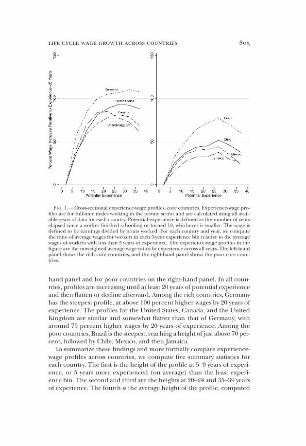
hand panel and for poor countries on the right-hand panel. In all coun-tries, profiles are increasing until at least 20 years of potential experienceand then flatten or decline afterward. Among the rich countries, Germanyhas the steepest profile, at above 100 percent higher wages by 20 years ofexperience. The profiles for the United States, Canada, and the UnitedKingdom are similar and somewhat flatter than that of Germany, witharound 75 percent higher wages by 20 years of experience. Among thepoor countries, Brazil is the steepest, reaching a height of just above 70 per-cent, followed by Chile, Mexico, and then Jamaica.To summarize these findings and more formally compare experience-
wage profiles across countries, we compute five summary statistics foreach country. The first is the height of the profile at 5–9 years of experi-ence, or 5 years more experienced (on average) than the least experi-ence bin. The second and third are the heights at 20–24 and 35–39 yearsof experience. The fourth is the average height of the profile, computed
FIG. 1.—Cross-sectional experience-wage profiles, core countries. Experience-wage pro-files are for full-time males working in the private sector and are calculated using all avail-able years of data for each country. Potential experience is defined as the number of yearselapsed since a worker finished schooling or turned 18, whichever is smaller. The wage isdefined to be earnings divided by hours worked. For each country and year, we computethe ratio of average wages for workers in each 5-year experience bin relative to the averagewages of workers with less than 5 years of experience. The experience-wage profiles in thefigure are the unweighted average wage ratios by experience across all years. The left-handpanel shows the rich core countries, and the right-hand panel shows the poor core coun-tries.

806 journal of political economy
as the average across all experience bins other than the lowest. The fifthis the average height when discounting each year at 4 percent per year,which is meant to be a simple measure of the discounted value of life-time income gains.4
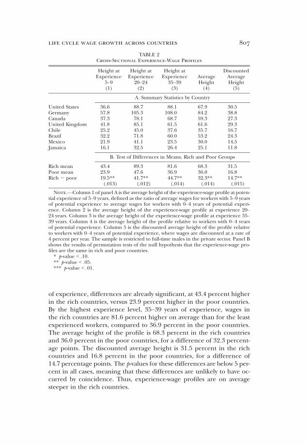
Panel A of table 2 reports the summary statistics for each country. Thereported heights are relative to the least experienced group, which com-prises workers with 0–4 four years of experience. Germany’s profile is thesteepest, reaching 105 percent by 20–24 years of experience. This is fol-lowed by the United States (90 percent), the United Kingdom (85 per-cent), and Canada (80 percent).5 Brazil’s profile is the steepest amongpoor countries, at approximately 70 percent. This is followed by Chile(45 percent), Mexico (40 percent), and Jamaica (33 percent). The heightsat 35–39 years of experience paint a similar picture, as do the average anddiscounted heights.Panel B of table 2 presents permutation tests of the null hypothesis
that experience-wage profiles are the same in the rich and poor coun-tries. The logic of the permutation test is that under the null, one canresample the data many times to compute the probability that one wouldobserve a difference as extreme as the actual difference in the data bychance. Permutation tests have better properties for small samples thanother commonly used tests, such as t -tests (Lehmann and Romano 2005).The differences between the means for rich countries and poor coun-
tries are large and statistically significant for all four of the summary sta-tistics. In the rich countries, the wages of workers with 20–24 years of ex-perience are 89.3 percent higher than those with less than 5 years ofexperience. In contrast, in the poor countries, the wages of workers with20–24 years of potential experience are just 47.6 percent higher thanthose with less than 5 years of experience. The difference is 41.7 percent-age points, which means that experience-wage profiles are roughly twiceas steep on average in rich countries by 20 years of experience.The profiles are also roughly twice as steep in rich countries according
to the other summary statistics. At the lowest experience level, 5–9 years
4 A convenient property of the discounted average height is that it appropriately tradesoff wage gains that occur early vs. late in life, and it therefore can be used, e.g., to comparethe profiles of two countries that cross. This summary statistic is also related to a statisticcommonly used to compute returns to education: the difference in the present discountedvalue of lifetime earnings across different education groups (see, e.g., Todaro and Smith[2012], sec. 8.2, and references cited there).
5 Our estimated experience-wage profiles for the rich countries are largely in line withprevious estimates in the literature. In the United States, e.g., Lemieux (2006) uses Cur-rent Population Survey data to estimate an increase in wages of 0.7 log points, or roughly100 percent, between 0 and 20 years of experience. Our estimates of other measures of lifecycle income growth, e.g., age-earnings profiles, also line up well with previous estimates inthe literature. Guvenen et al. (2014) use administrative data to estimate 127 percent higheraverage earnings for those aged 51 than those aged 25. Using our data, we calculate116 percent higher average earnings for those aged 51 than those aged 25.
life cycle wage growth across countries 807
of experience, differences are already significant, at 43.4 percent higherin the rich countries, versus 23.9 percent higher in the poor countries.By the highest experience level, 35–39 years of experience, wages inthe rich countries are 81.6 percent higher on average than for the leastexperienced workers, compared to 36.9 percent in the poor countries.The average height of the profile is 68.3 percent in the rich countriesand 36.0 percent in the poor countries, for a difference of 32.3 percent-age points. The discounted average height is 31.5 percent in the richcountries and 16.8 percent in the poor countries, for a difference of14.7 percentage points. The p-values for these differences are below 5 per-cent in all cases, meaning that these differences are unlikely to have oc-curred by coincidence. Thus, experience-wage profiles are on averagesteeper in the rich countries.
TABLE 2Cross-Sectional Experience-Wage Profiles
Height atExperience
5–9(1)
Height atExperience
20–24(2)
Height atExperience
35–39(3)
AverageHeight(4)
DiscountedAverageHeight(5)
A. Summary Statistics by Country
United States 36.6 88.7 88.1 67.9 30.5Germany 57.8 105.3 108.0 84.2 38.8Canada 37.3 78.1 68.7 59.3 27.3United Kingdom 41.8 85.1 61.5 61.6 29.3Chile 25.2 45.0 37.6 35.7 16.7Brazil 32.2 71.8 60.0 53.2 24.3Mexico 21.9 41.1 23.5 30.0 14.5Jamaica 16.1 32.5 26.4 25.1 11.8
B. Test of Differences in Means, Rich and Poor Groups
Rich mean 43.4 89.3 81.6 68.3 31.5Poor mean 23.9 47.6 36.9 36.0 16.8Rich 2 poor 19.5** 41.7** 44.7** 32.3** 14.7**
(.013) (.012) (.014) (.014) (.015)
Note.—Column 1 of panel A is the average height of the experience-wage profile at poten-tial experience of 5–9 years, defined as the ratio of average wages for workers with 5–9 yearsof potential experience to average wages for workers with 0–4 years of potential experi-ence. Column 2 is the average height of the experience-wage profile at experience 20–24 years. Column 3 is the average height of the experience-wage profile at experience 35–39 years. Column 4 is the average height of the profile relative to workers with 0–4 yearsof potential experience. Column 5 is the discounted average height of the profile relativeto workers with 0–4 years of potential experience, where wages are discounted at a rate of4 percent per year. The sample is restricted to full-time males in the private sector. Panel Bshows the results of permutation tests of the null hypothesis that the experience-wage pro-files are the same in rich and poor countries.* p -value < .10.** p -value < .05.*** p -value < .01.
808 journal of political economy
Finally, a point worth emphasizing is that virtually the entire differ-ence in steepness between rich and poor countries occurs over the first20 years of workers’ potential experience. For instance, panel B of table2 shows that 41.7 of the 44.7 percentage point mean difference betweenrich and poor countries in the height of the experience profiles is due topotential experience increasing from 0–4 to 20–24 years, and only an ad-ditional 3 percentage points are due to potential experience increasingfurther to 35–39 years. This fact is also apparent visually from figure 1. Inonline appendix A.3, we explore in more detail at what point of the lifecycle the differences in returns to experience between rich and poorcountries occur and show that about half of the difference in profilesat 20–24 years of experience is realized after only 5 years.
B. Experience-Wage Profiles for All Countries
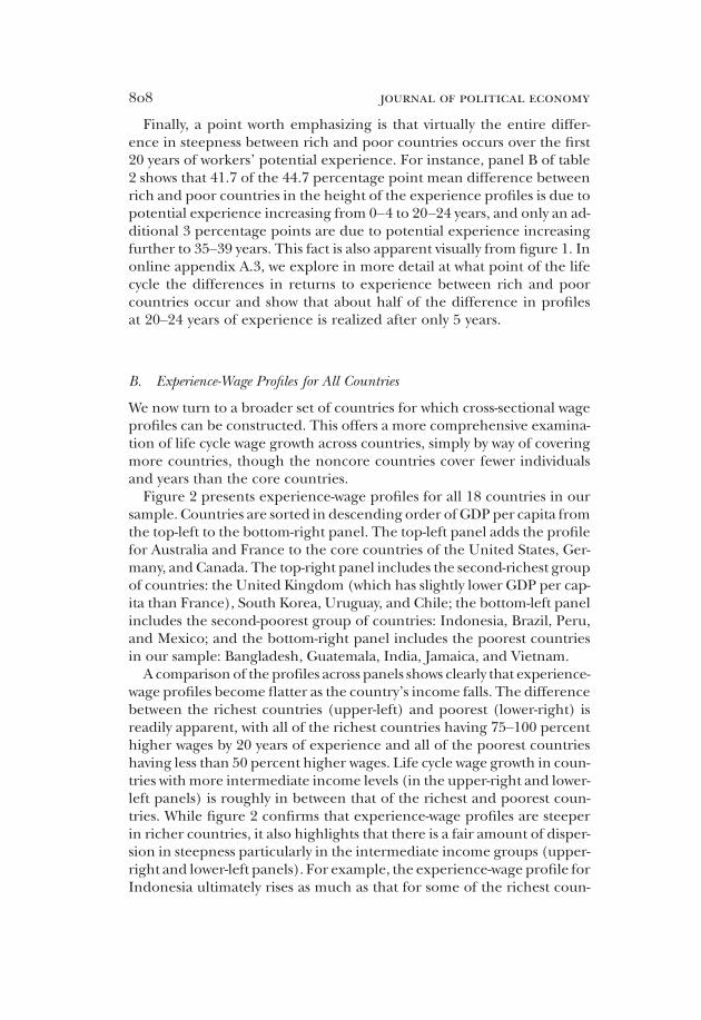
We now turn to a broader set of countries for which cross-sectional wageprofiles can be constructed. This offers a more comprehensive examina-tion of life cycle wage growth across countries, simply by way of coveringmore countries, though the noncore countries cover fewer individualsand years than the core countries.Figure 2 presents experience-wage profiles for all 18 countries in our
sample. Countries are sorted in descending order of GDPper capita fromthe top-left to the bottom-right panel. The top-left panel adds the profilefor Australia and France to the core countries of the United States, Ger-many, and Canada. The top-right panel includes the second-richest groupof countries: the United Kingdom (which has slightly lower GDP per cap-ita than France), South Korea, Uruguay, and Chile; the bottom-left panelincludes the second-poorest group of countries: Indonesia, Brazil, Peru,and Mexico; and the bottom-right panel includes the poorest countriesin our sample: Bangladesh, Guatemala, India, Jamaica, and Vietnam.A comparisonof the profiles across panels shows clearly that experience-
wage profiles become flatter as the country’s income falls. The differencebetween the richest countries (upper-left) and poorest (lower-right) isreadily apparent, with all of the richest countries having 75–100 percenthigher wages by 20 years of experience and all of the poorest countrieshaving less than 50 percent higher wages. Life cycle wage growth in coun-tries withmore intermediate income levels (in the upper-right and lower-left panels) is roughly in between that of the richest and poorest coun-tries. While figure 2 confirms that experience-wage profiles are steeperin richer countries, it also highlights that there is a fair amount of disper-sion in steepness particularly in the intermediate income groups (upper-right and lower-left panels). For example, the experience-wage profile forIndonesia ultimately rises as much as that for some of the richest coun-
life cycle wage growth across countries 809
tries. Nevertheless, on average, the overall pattern that experience-wageprofiles are steeper in richer countries remains: taking an average acrossall rich countries (in the core and full samples), the average height at 20–24 years of experience is 83.5 percent. For the poor countries, the averageis 45.9 percent, which results in a difference between rich and poor coun-tries of 37.5 percentage points. This difference is statistically significantat the 1 percent level and comparable in magnitude to the difference inthe core sample. Thus, figure 2 shows that the finding that experience-wage profiles are steeper in richer countries is true in the full sample aswell as in the sample of core countries. Finally, as already noted in the pre-vious section, the majority of the differences in profiles between rich andpoor countries occur over the first 20 years of workers’ life cycle.A complementary way to present the data is to look at the height of the
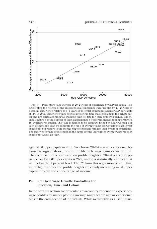
profiles at one particular experience level by GDP per capita. Figure 3plots the heights of the profiles after 20–24 years of potential experience
FIG. 2.—Cross-sectional experience-wage profiles, all countries. Experience-wage pro-files are for full-time males working in the private sector and are calculated using all avail-able years of data for each country. Potential experience is defined as the number of yearselapsed since a worker finished schooling or turned 18, whichever is smaller. The wage isdefined to be earnings divided by hours worked. For each country and year, we computethe ratio of average wages for workers in each 5-year experience bin relative to the averagewages of workers with less than 5 years of experience. The experience-wage profiles in thefigure are the unweighted average wage ratios by experience across all years. Countries aresorted in order of 2011 PPP GDP per capita from the top-left to the bottom-right panel.
810 journal of political economy
against GDP per capita in 2011. We choose 20–24 years of experience be-cause, as argued above, most of the life cycle wage gains occur by then.The coefficient of a regression on profile heights at 20–24 years of expe-rience on log GDP per capita is 26.2, and it is statistically significant atwell below the 1 percent level. The R 2 from this regression is .70. Thus,as the figure shows, the profile heights are clearly increasing in GDP percapita through the entire range of income.
IV. Life Cycle Wage Growth: Controlling forEducation, Time, and Cohort
In the previous section, we presented cross-country evidence on experience-wage profiles by simply plotting average wages within age or experiencebins in the cross section of individuals. While we view this as a useful start-
FIG. 3.—Percentage wage increase at 20–24 years of experience by GDP per capita. Thisfigure plots the heights of the cross-sectional experience-wage profiles by 20–24 years ofpotential experience relative to 0–4 years of potential experience against GDP per capitaat PPP in 2011. Experience-wage profiles are for full-time males working in the private sec-tor and are calculated using all available years of data for each country. Potential experi-ence is defined as the number of years elapsed since a worker finished schooling or turned18, whichever is smaller. The wage is defined to be earnings divided by hours worked. Foreach country and year, we compute the ratio of average wages for workers in each 5-yearexperience bin relative to the average wages of workers with less than 5 years of experience.The experience-wage profiles used in the figure are the unweighted average wage ratios byexperience across all years.
life cycle wage growth across countries 811
ing point because it imposes minimal structure and assumptions on thedata, there are a number of important issues that such a simple exercisedoes not address. First, our cross-sectional profiles ignore the role ofschooling. Second, cross-sectional estimates leave open the possibilitythat experience-wage profiles are driven by cohort effects, such as im-provements in the health of subsequent birth cohorts. In this sectionwe address both of these issues.Throughout this section, we estimate flexible versions of Mincer re-
gressions of individuals’ wages on their years of schooling and potentialexperience. That is, we estimate equations of the form
log wict 5 a 1 vsict 1 f xictð Þ 1 gt 1 wc 1 εict , (1)
where wict is the wage of individual i, who is a member of birth cohort cand is observed at time t; sict and xict are her years of schooling and expe-rience; gt is a vector of time period dummy variables; wc is a vector of co-hort dummy variables; and εict is a mean zero error term. We follow thetextbook specification and assume that schooling and experience enterin an additively separable fashion. This assumption is relaxed in Sec-tion VI.A, where we allow the returns to experience to differ betweenmoreand less educated workers. In what follows, we estimate equation (1) sep-arately for each country under various assumptions on cohort and timeeffects and then assess how the function f(⋅) varies across countries. Equa-tion (1) differs from the traditional Mincer regression in two ways. First,we allow the relationship between experience and wages to be flexible anddo not restrict the functional form to be linear. Second, we allow for co-hort and time effects, as we describe below.
A. Deaton-Hall Approach
The main challenge to estimating returns to experience (or age) is thatone cannot separately identify the effects of experience, birth cohort,and time because of collinearity. In this section, we consider the effectsof cohort and time controls following the approach proposed by Hall(1968) and Deaton (1997) for estimating returns to experience using re-peated cross sections. The main purpose of the Deaton-Hall approach isto illustrate themechanics of the econometric difficulty. The next sectionthen provides a theoretically motivated method for disciplining time andcohort effects. Before proceeding, we note that panel data would notsolve this identification problem. The reason is that even when followingspecific individuals (rather than cohorts) over time, one cannot separatehow much of their wage growth is due to aging or the passing of time. Ineither cross-sectional or panel data these effects can be identified only
812 journal of political economy
with additional assumptions, which, as is well known in the literature, areidentical for both types of data.6
To implement (1), we regress the logarithm of wages on schooling anda set of dummy variables for 5-year experience groups,
log wict 5 a 1 vsict 1 ox∈X
fxDxict 1 gt 1 xc 1 εict , (2)
in combination with one additional linear restriction on the set of cohortand time effects corresponding to different versions of the Deaton-Hallapproach. The term Dx
ict is a dummy variable that takes the value of oneif a worker is in experience group x ∈ X 5 f5–9, 10–14, : : :g; the omit-ted category is experience less than 5 years. This specification allows usto capture nonlinearities in a flexible way. The coefficient fx estimatesthe average wage of workers in experience group x relative to the averagewage of workers with less than 5 years of experience. In terms of our no-tation of equation (1), the fx terms represent f(x) such that the coeffi-cient estimate corresponding to each experience level, x, identifies theexperience-wage profile evaluated at point x.To resolve the difficulty of collinearity, Hall (1968) and Deaton (1997)
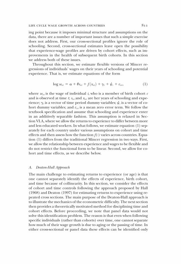
impose one additional linear restriction on the set of cohort and time ef-fects in equation (2). We consider three different versions of the Deaton-Hall approach. The first version attributes all labor productivity growthto cohort effects and uses year dummies to capture only cyclical fluctua-tions. This is the assumption made in Deaton’s (1997) original analysisand more recently by Aguiar and Hurst (2013). We implement this by es-timating equation (2) with birth cohort dummies and time dummies,with the restriction that the time dummies are orthogonal to a time trend.See online appendix A.2 for a more formal description of our methodol-ogy. The second version takes the opposite extreme and attributes all laborproductivity growth to time effects. We implement this by estimating equa-tion (2) with cohort and time dummies, but now we restrict the cohort ef-fects to be orthogonal to a time trend. The third takes the intermediateview that productivity growth is attributed in equal parts to cohort and timeeffects. While we are agnostic on the most natural split between time andcohort effects, the case of an equal split is nonetheless useful for illustrat-ing how the estimated returns to experience across countries depend onthe relative importance of the two effects.Figure 4A plots the estimates from the first version, in which all in-
come growth is attributed to cohort effects.7 The left-hand panel shows
6 For example, Heckman and Robb (1985, 140) note that “it is by now well known (Ca-gan 1973) that [panel] data do not solve the identification problem” and that “panel dataand a time series of cross sections of unrelated individuals are equally informative.”
7 The confidence intervals tend to be narrow for most countries, so we omit them forbrevity.
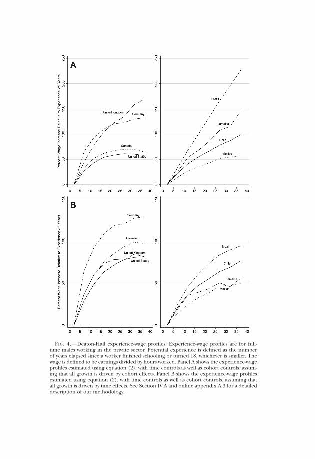
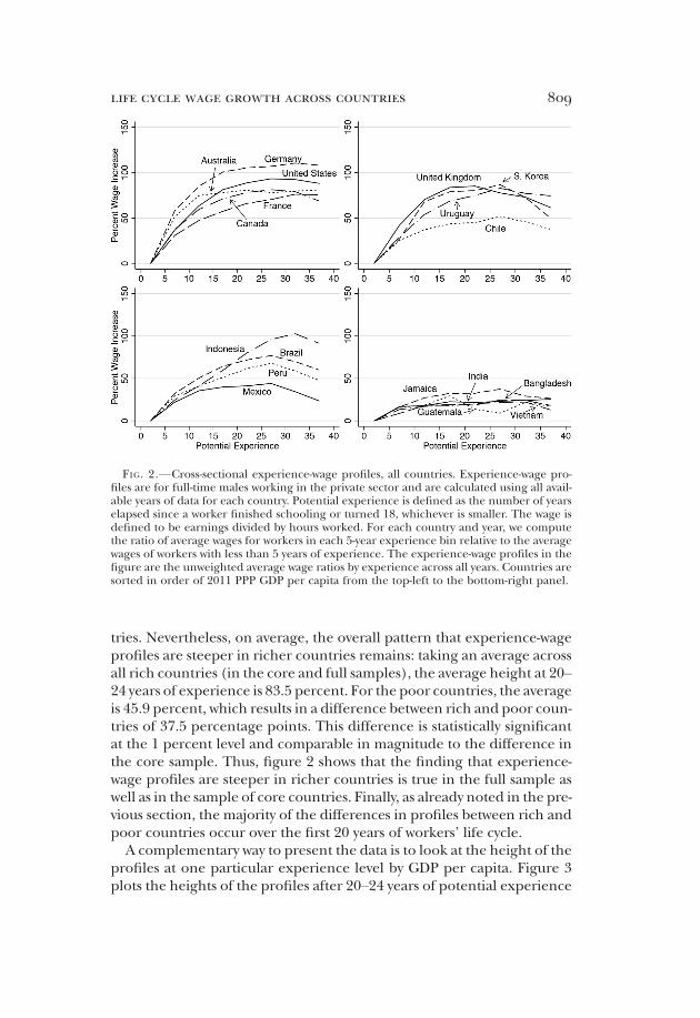
FIG. 4.—Deaton-Hall experience-wage profiles. Experience-wage profiles are for full-time males working in the private sector. Potential experience is defined as the numberof years elapsed since a worker finished schooling or turned 18, whichever is smaller. Thewage is defined to be earnings divided by hours worked. Panel A shows the experience-wageprofiles estimated using equation (2), with time controls as well as cohort controls, assum-ing that all growth is driven by cohort effects. Panel B shows the experience-wage profilesestimated using equation (2), with time controls as well as cohort controls, assuming thatall growth is driven by time effects. See Section IV.A and online appendix A.3 for a detaileddescription of our methodology.
814 journal of political economy
that Germany and the United Kingdom have the steepest profiles, withmore than 100 percent growth by 20 years of experience, while the UnitedStates and Canada have around 60 percent growth by 20 years of experi-ence. The right-hand panel shows that all of the poor countries have steepand linear (or close to linear) experience profiles, with Brazil being thesteepest, followed by Jamaica, Chile, and then Mexico. The reason thatthis version has such steep profiles is that, with time effects shut down,all wage growth by individual cohorts over their lifetimes is attributed totheir increased experience. In countries such as Brazil and Jamaica thathave experienced high rates of aggregate growth over this period, the sizeof the effects attributed to experience is large.8
Figure 4B plots the estimates from the second version, in which all la-bor productivity growth is attributed to time effects. The left-hand panelshows that Germany is still the highest, at more than 100 percent growth,while Canada, the United Kingdom, and the United States are close be-hind at between 75 percent and 90 percent growth. The right-hand panelshows that the poor countries have flatter profiles than the rich coun-tries, with Brazil still highest at around 70 percent growth, followed byChile at 65 percent growth and Mexico and Jamaica at just under 50 per-cent growth. These profiles are very similar to the cross-sectional profilesin Section III because both sets of profiles attribute wage growth overtime to changes in aggregate economic conditions rather than to im-provements across cohorts.Panel A of table 3 reports the five summary statistics when all growth
is explained by cohort effects. By 5–9 years of experience, profiles are18.3 percentage points higher in the rich than in the poor countries (andstatistically significant). By 20–24 years of experience, profiles are, on av-erage, 10.8 percentage points higher in the rich countries, and by 35–39 years the difference is 38.8 percentage points (though neither differ-ence is statistically significant). The average and discounted heights areslightly higher in the rich countries, but themagnitudes are small and sta-tistically insignificant.Panel B of table 3 shows the intermediate case in which growth is ex-
plained equally by cohort and time effects. By 5–9 years of experience,the difference is 20.2 percentage points and is statistically significant atthe 5 percent level. By 20–24 years of experience, the richmean is 27.4 per-centage points higher than the poor country mean, which is significant atthe 10 percent level. By 35–39 years of experience, rich and poor countrieshave similar means. The average height is 16.1 percentage points higheramong the rich, while the discounted height is 9.0 percentage points higher
8 Brazil and Jamaica had wage growth of 3.5 percent per year and 2.1 percent per year onaverage, while Chile and Mexico had growth of 1.6 percent and 1.1 percent. Among therich countries, the United Kingdom and Germany had wage growth of 2.0 and 1.9 percent,while Canada and the United States had average wage growth of 0.5 percent.

life cycle wage growth across countries 815
among the rich, with the latter being statistically significant at the 10 per-cent level.Panel C of table 3 reports the results when all growth is explained by
time effects. Themean for rich countries is 22.2 percentage points higherby 5–9 years, 44.4 percentage points higher by 20–24 years, and 31.1 per-centage points higher by 35–39 years. The average height is 31.6 percent-age points higher for the rich countries, while the discounted height is15.0 percentage points higher. All differences are statistically significantat the 5 percent level except for the height at 35–39 years.
TABLE 3Deaton-Hall Eperience-Wage Profiles
Height atExperience
5–9(1)
Height atExperience
20–24(2)
Height atExperience
35–39(3)
AverageHeight(4)
DiscountedAverageHeight(5)
A. All Growth Explained by Cohort Effects
Rich mean 42.6 90.9 94.1 70.9 32.0Poor mean 24.3 80.1 132.7 70.5 28.9Rich 2 poor 18.3** 10.8 238.7 .4 3.1
(.04) (.352) (.839) (.489) (.365)
B. Growth Explained Equally by Cohort and Time Effects
Rich mean 42.4 93.2 96.7 72.7 32.7Poor mean 22.2 65.8 99.5 56.6 23.7Rich 2 poor 20.2** 27.4* 22.8 16.1 9.0*
(.030) (.082) (.562) (.106) (.089)
C. All Growth Explained by Time Effects
Rich mean 41.9 95.8 101.1 75.0 33.6Poor mean 19.7 51.4 69.9 43.4 18.6Rich 2 poor 22.2** 44.4** 31.1 31.6** 15.0**
(.016) (.029) (.117) (.042) (.024)
Note.—This table reports summary statistics of experience-wage profiles estimated us-ing the Deaton-Hall method under the assumptions that all growth is driven by cohort ef-fects (panel A), growth is equally explained by cohort and time effects (panel B), and allgrowth is driven by time effects (panel C). The rows present the average of the rich coun-tries, the average of the poor countries, and the difference between the rich and poormeans,plus the results of permutation tests of the null hypothesis that the experience-wage profilesfor rich and poor are the same. Column 1 is the average height of the experience-wage pro-file at potential experience of 5–9 years, defined as the ratio of average wages for workerswith 5–9 years of potential experience to average wages for workers with 0–4 years of poten-tial experience. Column 2 is the average height of the experience-wage profile at experience20–24 years. Column 3 is the average height of the experience-wage profile at experience35–39 years. Column 4 is the average height of the profile relative to workers with 0–4 yearsof potential experience. Column 5 is the discounted average height of the profile relativeto workers with 0–4 years of potential experience, where wages are discounted at a rate of4 percent per year.* p -value < .10.** p -value < .05.*** p -value < .01.
816 journal of political economy
We conclude that if cohort effects explain all of growth, the profiles ofthe rich countries are marginally steeper than those of the poor coun-tries we observe. If, however, time effects explain half or more of growth,then experience-wage profiles are steeper in rich countries than in poorcountries, with differences that are statistically and economically signif-icant. Thus, we next ask whether economic theory can help us furtherdiscipline these profiles.
B. Heckman-Lochner-Taber Approach: No Growth at theEnd of the Life Cycle
The insight from the previous illustration is that the interpretation of thecross-sectional results depends on the extent to which aggregate growthis attributable to time or cohort effects. In this section, we propose a the-oretically motivated method for disentangling the relative importance oftime and cohort effects. In particular, we draw on the basic prediction of alarge number of theories of life cycle wage growth that there should belittle or no growth in the final years of a worker’s career. This predictionis shared by the three basicmechanisms for explaining life cycle wage pro-files emphasized in the literature, namely, human capital investment, search,and learning.9 The basic idea of our approach is to use the assumptionthat there are no experience effects in the final working years as a restric-tion to identify time effects and cohort effects. A similar reasoning has beenused by Heckman, Lochner, and Taber (1998), so we refer to this as theHeckman-Lochner-Taber (HLT) approach, though credit is due morebroadly, as variants of this idea have appeared in the works of McKenzie(2006), Huggett, Ventura, and Yaron (2011), Bowlus and Robinson (2012),and Schulhofer-Wohl (2013).10
A simple example helps motivate how this method identifies the effectof wages due to experience (or age) rather than time or cohort. Imaginethat we follow the wages of two cohorts: a “young cohort” that has 0–4 yearsof experience in the year 2000 and an “old cohort” that has 30–34 years ofexperience in the year 2000. Say we observe that the young cohort has wagegrowth of 5 percent between 2000 and 2005, while the old cohort hasgrowth of only 1 percent over the same period. Under the assumption that
9 See, e.g., the review by Rubinstein and Weiss (2006).10 Heckman et al. (1998) and Bowlus and Robinson (2012) have used a similar insight in
models of human capital to separate prices and quantities of human capital, and Huggettet al. (2011) have used the assumption of no human capital investment at the end of thelife cycle to identify shocks to human capital. McKenzie (2006) shows that when using re-peated cross-sectional data, second differences of age, cohort, and time effects are identi-fied without any assumptions and that first differences can be identified as well with a re-striction on one first difference. Our method selects one such restriction using economictheory. Similarly, Schulhofer-Wohl (2013) argues that one should use the curvature of wageprofiles to identify parameters of structural models.
life cycle wage growth across countries 817
the old cohort has no wage growth coming through experience, the differ-ence in the time effects between 2000 and 2005 must be 1 percent. Thus,we infer that the young cohort had wage increases of 4 percent (5 2 1)coming from their increased experience. Repeating this idea for manycohorts, we can build up a full series of time effects. Given time effects,we can then estimate the remaining cohort and life cycle age or experienceeffects. This method is easily extended to allow for depreciation of skills orof match quality at the end of life. In this case, we replace the assumptionthat age/experience effects are zero with the assumption that they are2d percent, where d is the depreciation rate. The rest of the method pro-ceeds as above.This approach requires assumptions about two main parameters: first,
the number of years at the end of the life cycle for which there are no ex-perience effects and, second, a number for the depreciation rate. We fol-low Huggett et al. (2011) and consider either 5 or 10 years with no expe-rience effects. We consider two alternative depreciation rates of either 0or 1 percent per year. Given the assumptions about the number of yearswithout experience effects, y, and a depreciation rate, d, this approach toestimating the experience-wage profile in a particular country works asfollows. First, we guess an initial trend in the time effects. We then de-flate wages for each individual in each year by the wage growth rate im-plied by the time effect. Next, we estimate equation (1) with experienceeffects and cohort effects, and we check whether the estimated experi-ence effects have declined, on average, by d percent in the last y years.If they have, we stop. Otherwise we adjust the trend in the time effectsand repeat. Once the process has converged, it produces separate esti-mates of cohort effects, time effects, and experience effects for a givencountry and for given values of y and d.For the purposes of our paper, there are two main benefits to this HLT
approach. First, it uses economic theory to motivate restrictions on timeand cohort effects. Second, it allows the sources of growth to be countryspecific, which is useful when comparing countries with very different in-come levels and growth rates.11
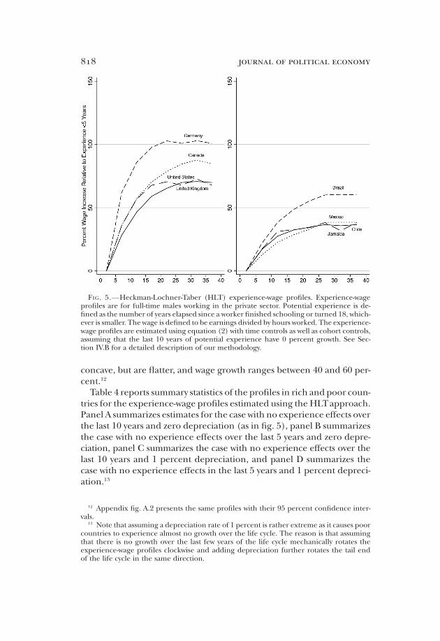
Figure 5 plots the experience-wage profiles estimated using the HLTmethod under the assumption that there are no experience effects inthe last 10 years of the life cycle and no depreciation. In the rich coun-tries, the experience-wage profiles are concave and grow by 70–100 per-cent by 20 years of experience. Profiles for the poor countries are also
11 Themost widely applied alternative theoretical restriction, proposed by Deaton (1997),restricts time effects to sum to zero, as in fig. 4A above. The theoretical rationale for this was“to use the year effects to capture cyclical fluctuations or business-cycle effects that average tozero over the long run” (126). This restriction is less relevant for our analysis given that oursample includes many fast-growing countries.
818 journal of political economy
concave, but are flatter, and wage growth ranges between 40 and 60 per-cent.12
Table 4 reports summary statistics of the profiles in rich and poor coun-tries for the experience-wage profiles estimated using the HLTapproach.Panel A summarizes estimates for the case with no experience effects overthe last 10 years and zero depreciation (as in fig. 5), panel B summarizesthe case with no experience effects over the last 5 years and zero depre-ciation, panel C summarizes the case with no experience effects over thelast 10 years and 1 percent depreciation, and panel D summarizes thecase with no experience effects in the last 5 years and 1 percent depreci-ation.13
FIG. 5.—Heckman-Lochner-Taber (HLT) experience-wage profiles. Experience-wageprofiles are for full-time males working in the private sector. Potential experience is de-fined as the number of years elapsed since a worker finished schooling or turned 18, which-ever is smaller. The wage is defined to be earnings divided by hours worked. The experience-wage profiles are estimated using equation (2) with time controls as well as cohort controls,assuming that the last 10 years of potential experience have 0 percent growth. See Sec-tion IV.B for a detailed description of our methodology.
12 Appendix fig. A.2 presents the same profiles with their 95 percent confidence inter-vals.
13 Note that assuming a depreciation rate of 1 percent is rather extreme as it causes poorcountries to experience almost no growth over the life cycle. The reason is that assumingthat there is no growth over the last few years of the life cycle mechanically rotates theexperience-wage profiles clockwise and adding depreciation further rotates the tail endof the life cycle in the same direction.

life cycle wage growth across countries 819
In all four panels the rich-poor country differences in heights at 5–9 years and 20–24 years of experience are large and statistically signifi-cant. The same is true for the heights at 35–39 years of experience, theaverage heights, and discounted average heights. The largest differencesare estimated under the assumption that there are no experience effectsin the last 5 years and no depreciation (panel B), while the differences
TABLE 4Heckman-Lochner-Taber (HLT) Experience-Wage Profiles
Height atExperience
5–9(1)
Height atExperience
20–24(2)
Height atExperience
35–39(3)
AverageHeight(4)
DiscountedAverageHeight(5)
A. No Experience Effects in Last 10 Years, 0% Depreciation
Rich mean 40.3 79.3 80.8 62.5 28.5Poor mean 17.2 39.2 43.3 31.3 14.0Rich 2 poor 23.1** 40.1** 37.5** 31.2** 14.5**
(.014) (.013) (.013) (.013) (.013)
B. No Experience Effects in Last 5 Years, 0% Depreciation
Rich mean 42.3 90.3 100.7 72.1 32.3Poor mean 16.0 33.2 33.1 26.2 12.0Rich 2 poor 26.3** 57.0** 67.6** 45.9** 20.3**
(.015) (.013) (.013) (.016) (.015)
C. No Experience Effects in Last 10 Years, 1% Depreciation
Rich mean 33.9 47.1 27.5 35.2 17.7Poor mean 12.1 14.3 1.3 10.0 5.6Rich 2 poor 21.8** 32.7** 26.2** 25.3** 12.2**
(.015) (.015) (.017) (.015) (.014)
D. No Experience Effects in Last 5 Years, 1% Depreciation
Rich mean 35.8 55.9 41.3 42.6 20.7Poor mean 10.9 9.4 26.0 5.9 3.9Rich 2 poor 24.9** 46.5** 47.3** 36.7** 16.8**
(.013) (.014) (.013) (.014) (.015)
Note.—This table reports summary statistics of the estimated experience-wage profilesestimated under the assumption that there are no experience effects in the last 10 years ofpotential experience and no depreciation (panel A), no experience effects in the last5 years and no depreciation (panel B), no experience effects in the last 10 years and 1 per-cent depreciation (panel C), and no experience effects in the last 5 years and 1 percentdepreciation (panel D). The rows present the average of the rich and poor countries, pluspermutation tests of the null hypothesis that rich and poor are the same. Column 1 is theaverage height of the experience-wage profile at potential experience of 5–9 years. Col-umns 2 and 3 are the same but for 20–24 and 35–39 years of potential experience. Col-umn 4 is the average height of the profile relative to workers with 0–4 years of potentialexperience. Column 5 is the discounted average height of the profile, relative to 0–4 yearsof experience, where wages are discounted at a rate of 4 percent per year.* p -value < .10.** p -value < .05.*** p -value < .01.
820 journal of political economy
are smallest when depreciation is 1 percent and there are no experienceeffects in the last 10 years (panel C). The reason is that when there is de-preciation, the profiles themselves are flatter in all countries; hence cross-country differences become smaller. In summary, the results in table 4show that the heights of the profiles can be sensitive to the depreciationrate or the length of time with no gains from experience. However, ourmain result that there are more life cycle wage gains in rich countriesis present in all cases.Similarly to the cross-sectional profiles in Section III.A, most of the dif-
ference in steepness between rich and poor countries occurs over thefirst 20 years of workers’ potential experience. For instance, panel Ashows that with no experience effects over the last 10 years and zero de-preciation, experience-wage profiles at 20–24 years are 40.1 higher inrich countries, and at 35–39 years they are 37.5 percent higher. Thatis, toward the end of the life cycle poor countries actually make up fora small part of the gap in the height of the profiles. Also see online ap-pendix A.3, where we explore this point in greater detail and show that,similarly to our cross-sectional results, about half of the difference inprofiles at 20–24 years of experience is realized after 5 years only.Note that the HLT results in table 4 are quite similar to the cross-
sectional estimates shown earlier in table 2. In light of the discussion inthe previous section, this is consistent withmost of the growth experiencedby the countries in our core sample being attributable to time effects.
V. Robustness
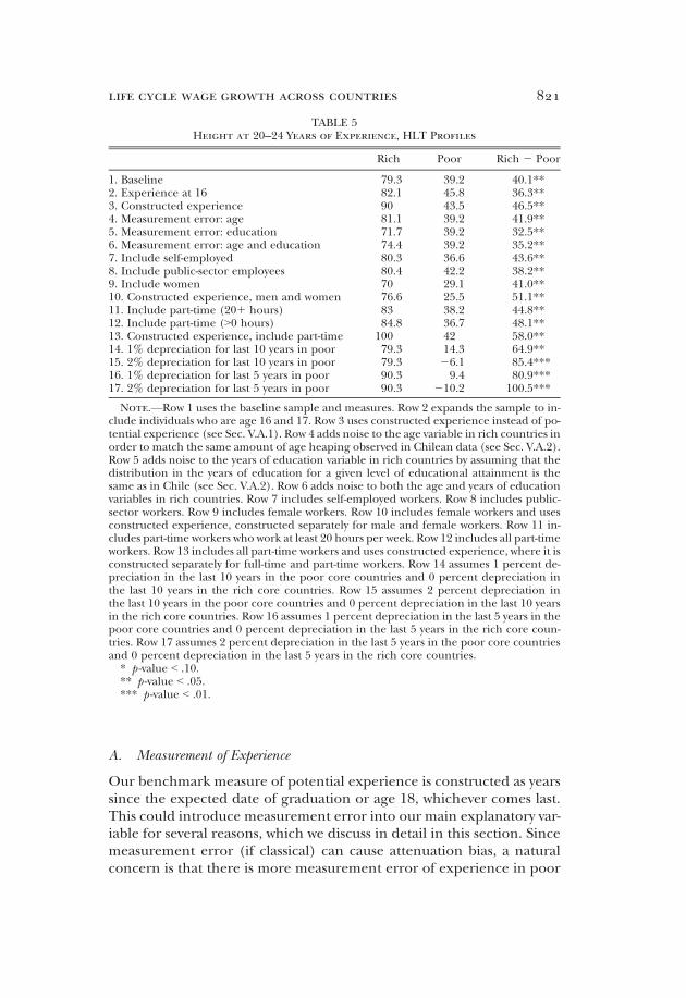
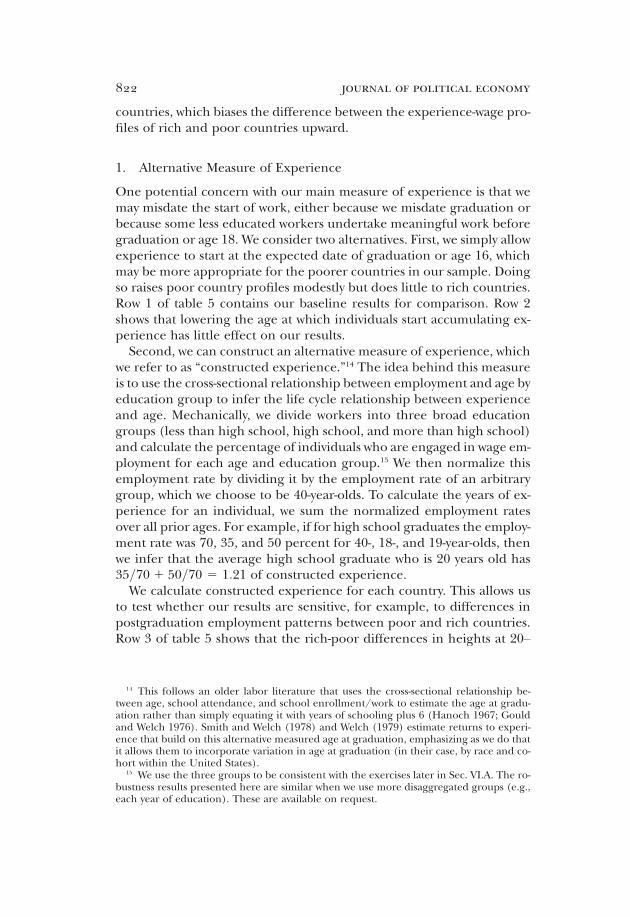
This section considers the robustness of our main finding that life cyclewage profiles are steeper in richer than in poorer countries. In particu-lar, we demonstrate that our main result that experience-wage profilesare steeper in rich countries is unlikely to be an artifact of how we mea-sure experience or restrict the sample. Unless otherwise stated, we focuson our preferred estimates that use the HLT method to decompose age,time, and cohort effects and restrict our attention to the core sample ofcountries.Most of our results are summarized in table 5. Each row corresponds
to an alternative sample selection criterion or variable construction. Wefocus on the heights of the profiles at 20–24 years of experience for brev-ity. The columns contain the average height across the four rich coun-tries, the average height across the four poor countries, and the differ-ence. We conducted similar analyses to verify that our cross-sectionalresults from Section III are also robust. See appendix table A.2, wherewe present the results for both the core sample of eight countries andthe full sample of 18 countries.
life cycle wage growth across countries 821
A. Measurement of Experience
Our benchmark measure of potential experience is constructed as yearssince the expected date of graduation or age 18, whichever comes last.This could introduce measurement error into our main explanatory var-iable for several reasons, which we discuss in detail in this section. Sincemeasurement error (if classical) can cause attenuation bias, a naturalconcern is that there is more measurement error of experience in poor
TABLE 5Height at 20–24 Years of Experience, HLT Profiles
Rich Poor Rich 2 Poor
1. Baseline 79.3 39.2 40.1**2. Experience at 16 82.1 45.8 36.3**3. Constructed experience 90 43.5 46.5**4. Measurement error: age 81.1 39.2 41.9**5. Measurement error: education 71.7 39.2 32.5**6. Measurement error: age and education 74.4 39.2 35.2**7. Include self-employed 80.3 36.6 43.6**8. Include public-sector employees 80.4 42.2 38.2**9. Include women 70 29.1 41.0**10. Constructed experience, men and women 76.6 25.5 51.1**11. Include part-time (201 hours) 83 38.2 44.8**12. Include part-time (>0 hours) 84.8 36.7 48.1**13. Constructed experience, include part-time 100 42 58.0**14. 1% depreciation for last 10 years in poor 79.3 14.3 64.9**15. 2% depreciation for last 10 years in poor 79.3 26.1 85.4***16. 1% depreciation for last 5 years in poor 90.3 9.4 80.9***17. 2% depreciation for last 5 years in poor 90.3 210.2 100.5***
Note.—Row 1 uses the baseline sample and measures. Row 2 expands the sample to in-clude individuals who are age 16 and 17. Row 3 uses constructed experience instead of po-tential experience (see Sec. V.A.1). Row 4 adds noise to the age variable in rich countries inorder to match the same amount of age heaping observed in Chilean data (see Sec. V.A.2).Row 5 adds noise to the years of education variable in rich countries by assuming that thedistribution in the years of education for a given level of educational attainment is thesame as in Chile (see Sec. V.A.2). Row 6 adds noise to both the age and years of educationvariables in rich countries. Row 7 includes self-employed workers. Row 8 includes public-sector workers. Row 9 includes female workers. Row 10 includes female workers and usesconstructed experience, constructed separately for male and female workers. Row 11 in-cludes part-time workers who work at least 20 hours per week. Row 12 includes all part-timeworkers. Row 13 includes all part-time workers and uses constructed experience, where it isconstructed separately for full-time and part-time workers. Row 14 assumes 1 percent de-preciation in the last 10 years in the poor core countries and 0 percent depreciation inthe last 10 years in the rich core countries. Row 15 assumes 2 percent depreciation inthe last 10 years in the poor core countries and 0 percent depreciation in the last 10 yearsin the rich core countries. Row 16 assumes 1 percent depreciation in the last 5 years in thepoor core countries and 0 percent depreciation in the last 5 years in the rich core coun-tries. Row 17 assumes 2 percent depreciation in the last 5 years in the poor core countriesand 0 percent depreciation in the last 5 years in the rich core countries.* p -value < .10.** p -value < .05.*** p -value < .01.
822 journal of political economy
countries, which biases the difference between the experience-wage pro-files of rich and poor countries upward.
1. Alternative Measure of Experience
One potential concern with our main measure of experience is that wemay misdate the start of work, either because we misdate graduation orbecause some less educated workers undertake meaningful work beforegraduation or age 18. We consider two alternatives. First, we simply allowexperience to start at the expected date of graduation or age 16, whichmay be more appropriate for the poorer countries in our sample. Doingso raises poor country profiles modestly but does little to rich countries.Row 1 of table 5 contains our baseline results for comparison. Row 2shows that lowering the age at which individuals start accumulating ex-perience has little effect on our results.Second, we can construct an alternative measure of experience, which
we refer to as “constructed experience.”14 The idea behind this measureis to use the cross-sectional relationship between employment and age byeducation group to infer the life cycle relationship between experienceand age. Mechanically, we divide workers into three broad educationgroups (less than high school, high school, and more than high school)and calculate the percentage of individuals who are engaged in wage em-ployment for each age and education group.15 We then normalize thisemployment rate by dividing it by the employment rate of an arbitrarygroup, which we choose to be 40-year-olds. To calculate the years of ex-perience for an individual, we sum the normalized employment ratesover all prior ages. For example, if for high school graduates the employ-ment rate was 70, 35, and 50 percent for 40-, 18-, and 19-year-olds, thenwe infer that the average high school graduate who is 20 years old has35=70 1 50=70 5 1:21 of constructed experience.We calculate constructed experience for each country. This allows us
to test whether our results are sensitive, for example, to differences inpostgraduation employment patterns between poor and rich countries.Row 3 of table 5 shows that the rich-poor differences in heights at 20–
14 This follows an older labor literature that uses the cross-sectional relationship be-tween age, school attendance, and school enrollment/work to estimate the age at gradu-ation rather than simply equating it with years of schooling plus 6 (Hanoch 1967; Gouldand Welch 1976). Smith and Welch (1978) and Welch (1979) estimate returns to experi-ence that build on this alternative measured age at graduation, emphasizing as we do thatit allows them to incorporate variation in age at graduation (in their case, by race and co-hort within the United States).
15 We use the three groups to be consistent with the exercises later in Sec. VI.A. The ro-bustness results presented here are similar when we use more disaggregated groups (e.g.,each year of education). These are available on request.
life cycle wage growth across countries 823
24 years of experience using constructed experience are, if anything,slightly larger than our baseline results.16
2. Measurement Error in Age or Education
Since potential experience is constructed using reported age and esti-mated years of schooling, mismeasurement of either variable that ismore pronounced in poor countries could cause the experience-wageprofiles of poor countries to attenuate more than that of rich countries.In particular, one may worry that survey respondents in poor countriesare more likely to round their ages or provide a noisy estimate of theiractual educational attainment. This could in principle lead to a spuriousfinding of flatter experience-wage profiles.When looking at reported age distributions in the poor core coun-
tries, we do observe that there is some age heaping in Mexico and Chile,where there are small spikes in population frequency at every 10 years ofage (see fig. A.6). To examine whether age heaping drives the differencebetween poor and rich country experience-wage profiles, we artificiallydistort the age distributions of rich countries to match the age heapingobserved in the Chilean data.17 We then reconstruct potential experi-ence using the distorted age data in each country and reestimate theexperience-wage profiles using ourHLTapproach.We find that with thesedistorted age data, the experience-wage profiles of the rich countries arevery similar to the actual profiles. Row4 in table 5 shows that with distortedages, the rich countries have an average height of 81.1 compared to the79.3 in the baseline. Artificially distorting the age distribution to replicatethe same level of age heaping observed in Chile makes the profile of Ger-many slightly steeper and the profiles of the United States, Canada, andthe United Kingdom marginally flatter (see app. fig. A.3). We concludethat it is unlikely thatmismeasurement of age plays an important role in ex-plaining our findings.
16 Note that interpreting the results using constructed experience relies on the assump-tion that patterns of work are consistent over time within a country: that if the average highschool graduate gains 0.5 year of experience at age 18 in 2001, the same was true for earliercohorts. We do not expect this assumption to hold exactly but nevertheless find it a usefulrobustness check as it allows us to present results that do not depend on assumptions aboutthe expected graduation date or the earliest possible age of work.
17 We estimate a smooth version of the age distribution in Chile using a quintic regres-sion and define age heaping as the difference between the actual age distribution and thesmoothed one. Equipped with the estimated age heaping level for each age, we turn backto the microdata from the rich countries and artificially distort them. For example, if weobserve that in Chile there are 5 percent fewer individuals aged 19 than expected accord-ing to the smoothed age distribution and 5 percent more individuals aged 20, then we ran-domly assign 5 percent of 19-year-olds to be 20 years old instead in each rich country. Thisexercise replicates, by construction, the same amount of age heaping as in Chile.
824 journal of political economy
To address concerns about measurement error in education, we turnto the Chilean data, where respondents were asked to report both thenumber of years they attended school and the highest level of attain-ment.18 The data show that there is indeed variation in the number of yearsof actual schooling for a given level of attainment (see app. table A.4). Forexample, in Chile, the years of schooling for someone who completed“some primary” range from 3 to 8 years. For those who complete “college,”the number of years varies only between 16 and 18 years. Thus, those whoreport having “some primary” range between 33 percent fewer and 100 per-cent more than the imputed number of years of schooling. And thosewho complete college range between 0 percent less and 12.5 percentmorethan the imputed number of years of schooling.To investigate whether this variability drives the steeper profiles in rich
countries, we impose the same dispersion onto the four rich countries inour core sample. Since the categories of educational attainment differacross surveys, we divide the data into three groups: less than high school,high school, andmore than high school. For each group, we use the datafromChile to calculate the averagepercentagedeviation from the imputedyears of schooling for each percentile. We then distort the data for the richcountries such that the dispersion in the years of schooling for each attain-ment level follows the Chilean distribution of the group that the level be-longs to, and we reestimate the experience-wage profiles with the distorteddata.We find that the data with distorted education levels yield experience-
wage profiles that are modestly flatter than the actual profiles. Table 5,row 5, shows that the mean for rich countries is 71.7 compared to 79.3in the benchmark. The difference with the poor countries is still large,at 32.5, and statistically significant at the 5 percent level. Therefore, at leastwith the measurement error in the Chilean data as a guide, mismeasure-ment of education is not likely to explain much of our findings.19
B. Sample Selection
Our baseline analysis focused on a sample that is designed to maximizecomparability between countries and minimize measurement concerns:
18 We focus on the Chilean data from 2009 since it is the most recent year, though similardata are available in 2000, 2003, and 2006. The Jamaican data from 1991 and 2001 alsoasked these questions. However, the quality of the data for years of education is poor: thereare many missing values and implausible responses (e.g., the number of years for thosewho report “no education” as their highest level of attainment ranges from 0 to 15 years).Thus, we do not use the data from Jamaica.
19 Appendix fig. A.4 presents the experience-wage profiles using the distorted and actualeducation data. We also estimated the profiles using distorted age and education data,finding profiles that were again only modestly flatter than those of the baseline analysis;see app. fig. A.5 and row 6 of table 5 for the rich-poor differences in profile heights.
life cycle wage growth across countries 825
full-time, private-sector male wage workers. This raises two questions.The first and most important for our study is the concern that the mainresult that experience-wage profiles are steeper for the sample of inter-est in richer countries is driven by differential selection into the sample.For example, if less productive workers select out of wage employment inrich countries as they age while such workers select into wage employ-ment in poor countries as they age, our finding of steeper profiles forwage workers could be driven by differential selection. The second ques-tion is whether the profiles will still be steeper once we relax the samplerestrictions and include other types of workers.20 In this section, we pro-vide evidence against the concern that selection is the main driving forceof our results and suggestive evidence that the profiles will still be steeperwhen we expand the sample. We explain our approach in detail for self-employed workers and then briefly overview the parallel results for public-sector workers, women, and part-time workers.
1. Self-Employed Workers
An important sample restriction is that we focus on wage earners becausewage income is a direct payment for labor services that is generally con-sidered to be accurately reported. In contrast, the income of the self-employed presents two challenges. First, it can represent payments forboth labor and capital services, implying that it is less directly related tolife cycle theories of human capital accumulation or search and match-ing. Second, it is well known that the reported incomeof the self-employedsuffers from substantial underreporting (Hurst et al. 2014).A concern with using only wage workers in repeated cross-sectional data
is that there may be selection into or out of self-employment over time.We address this concern in several ways. One is to simply include theseworkers in our estimates. In row 7 of table 5, we show the result from in-cluding the self-employed, taking their reported income to be their wageand salary income. Doing so has little effect on our results.The caveat for interpreting this result is that proxying for wages this
way introduces measurement error for the reasons discussed earlier.To address this, we use panel data. Since panel data are not widely avail-able, we choose one rich country, the United States (Panel Study of In-come Dynamics [PSID], annually 1975–97, biannually 1999–2013), andone poor country, Mexico (Mexican Family Life Survey [FLS], 2002,2005, and 2009). In the main analysis, US workers have very steep pro-
20 Note that for the eight core countries, the size of our sample as a percentage of totalmale workers is 63 percent in the United States, 66 percent in the United Kingdom, 65 per-cent in Mexico, 45 percent in Jamaica, 67 percent in Germany, 70 percent in Chile, 67 per-cent in Canada, and 61 percent in Brazil.

826 journal of political economy
files, while Mexican workers have flat profiles. Thus, they are useful forunderstanding whether selection into or out of self-employment causesprofiles in rich countries to be steeper. Moreover, to the best of ourknowledge, Mexico is the only poor country within our core sample tohave panel data. As with the main exercise, we examine male full-timeworkers in the private sector.Experience-wage profiles following the same individuals.—First, we show that
the estimated experience-wage profiles from panel data are similar tothose from repeated cross sections. To be transparent, we employ a non-parametric approach and simply follow individuals over time withoutcontrolling for time fixed effects. Since the Mexican FLS data are avail-able only for the years 2002, 2005, and 2009, we use waves of the PSID froma comparable time period, 2003–13. The sample is restricted to individualswho were present during all of the specified waves for the surveys.We divide the sample into cohorts based on the level of potential expe-
rience in the first year of the data (i.e., 2002 for the FLS and 2003 for thePSID). As with the main exercise, a cohort group comprises 5 years of ex-perience levels (e.g., the youngest cohort in Mexico had 0–4 years of ex-perience in 2002). We then calculate the average wage for each bin andnormalize it by dividing it by the average wage of the youngest cohort thatyear.Figure 6A shows that the US profile is higher than theMexican profile.
Each line segment in the figure is the normalized wage of a cohort overtime. Figure 6B shows the analogous profiles from the repeated cross-sectional data (these are identical to those in fig. 1). A comparison ofthe two figures shows that the panel and repeated cross-sectional dataare broadly similar.Selection into and out of wage employment.—Another concern is that our
results are driven by differential selection into (or out of) our sampleacross countries. In online appendix A.4 we use the panel data describedabove from the United States and Mexico to show that this is unlikely.Specifically, we show that selection into or out of wage employment,private-sector employment, and full-time employment has negligible ef-fects on the estimated relationship between experience and wages in theUnited States and Mexico.
2. Other Sample Selection
In this section we quantify the importance of the remaining sample se-lection criteria, using many of the same techniques introduced at lengthin the previous section. We start with the restriction to private-sectorworkers. Row 8 of table 5 shows that our results are very similar if we in-clude public-sector employees. We then repeat the same analysis using
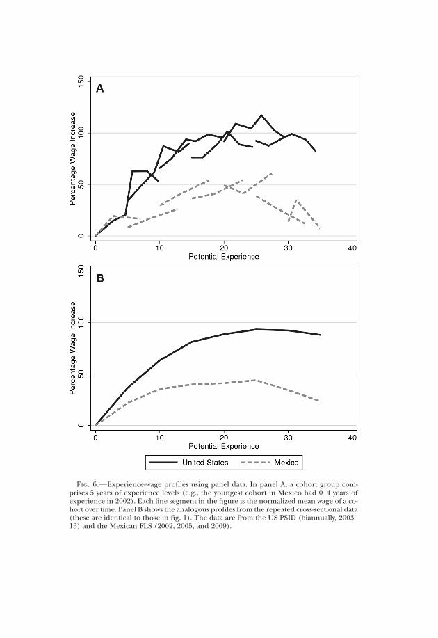
FIG. 6.—Experience-wage profiles using panel data. In panel A, a cohort group com-prises 5 years of experience levels (e.g., the youngest cohort in Mexico had 0–4 years ofexperience in 2002). Each line segment in the figure is the normalized mean wage of a co-hort over time. Panel B shows the analogous profiles from the repeated cross-sectional data(these are identical to those in fig. 1). The data are from the US PSID (biannually, 2003–13) and the Mexican FLS (2002, 2005, and 2009).
828 journal of political economy
panel data to compare workers who remain private-sector workers tothose who switch to or from public-sector employment. We find thatthere is no obvious pattern over the life cycle, and the flow of workers fromone sector to the other is very low such that selection into and out of theprivate sector can have only negligible effects on our estimates; the detailsand figures are in online appendix A.5. Finally, we find that public-sectoremployment is unlikely to drive our results because very few workers areemployed in the public sector: on average, 8 percent in the rich countriesin our sample and 3 percent in the poor countries in our sample.We next turn to female workers, who were excluded from the baseline
analysis. Table 5, row 9, shows the results if we include female full-timeworkers in the private sector. The results are very similar to the baselinein row 1. We do not use the panel data approach employed elsewheresince gender is a fixed characteristic, and we therefore are not worriedabout women transitioning in and out of our sample as we are for theself-employed. Instead, we consider robustness to measuring women’sexperience using constructed experience as in Section V.A.1 rather thanpotential experience; this helps address the concern that potential expe-rience may not accurately reflect the women’s actual experience if theyare more likely to experience career interruptions. The results in row 10show that this actually increases the gap in the heights of experience pro-files between rich and poor countries.Finally, we investigate the importance of the exclusion of part-time
workers (those who work less than 30 hours a week). Rows 11 and 12of table 5 show that the estimates change little when we include workerswho work at least 20 hours a week or all part-time workers (i.e., workerswho report any wage income). Row 13 shows the results when we useconstructed experience, where this measure is constructed for full-timeand part-time workers separately. The results are very similar to the base-line. Finally, in online appendix A.5 we study the experience profiles ofworkers who switch between part-time and full-time work. We find thatsuch switches are common but have little effect on the profiles, suggest-ing that they are unlikely to drive our results.
C. Alternative Assumptions about Depreciationat the End of the Life Cycle
Our implementation of the HLT method relies on the assumption thatwage movements near the end of the working life can be attributed todepreciation rates. We started with the natural assumption that the de-preciation rate was common across countries. In this section we considerrelaxing that assumption and allowing the depreciation rate of humancapital to differ across countries. In order to discipline this analysis, welink possible variation in the depreciation rate to the type of jobs done.

life cycle wage growth across countries 829
As we will document below in Section VII, most workers in rich countriesare engaged in occupations that use their learned knowledge, whereasaround half of workers in poor countries are engaged in occupations thatuse physical strength and stamina. This leads us to discipline the analysisthrough the age-related decline in mental and physical performance.For the former, we draw on a large literature that documents the life
cycle performance of athletes who compete in track and field events onan age-adjusted basis (Tanaka and Seals 2008). Consistent with the model,we study the decline in record performance (measured as distance ortime) between ages 60–64 and ages 65–69, downloaded from World Mas-ters Athletics Current Records (http://www.world-masters-athletics.org/records/current-records). Peak performance declines in all categories,with themedian andmeandepreciation agreeing closely at 1.2 and 1.3 per-cent. For the depreciation of knowledge we turn to the corresponding psy-chological literature, which generally focuses on vocabulary knowledge orother forms of related, easy-to-measure knowledge. The stylized finding inthis literature is that learnedknowledge grows until roughly age 60, withnolarge changes for the subsequent 10 years, implying that knowledge depre-ciation is 0 percent at least through age 70 (Salthouse 2003, 2013).We consider four additional robustness checks based on these find-
ings. In each, we fix the depreciation rate in rich countries at 0 percent.We consider allowing the depreciation rate in poor countries to be 1 or2 percent for 5 or 10 years, motivated by the depreciation of physicalstrength and stamina. The results are given in rows 14–17 of table 5.The main result is that these robustness checks flatten out experienceprofiles in poor countries, which serves only to increase the gap betweenpoor and rich countries. We conclude that restricting depreciation ratesto be the same in poor and rich countries is probably a conservative as-sumption.
VI. Interactions between Schooling and Experience
In this section, we allow for interactions between schooling and age or ex-perience and ask what fraction of cross-country differences in aggregatewage profiles is accounted for by cross-country differences in educationlevels.
A. Experience-Wage Profiles by Schooling Level
We have so far presented experience-wage profiles under the standardassumption that returns to experience do not vary by educational attain-ment. We now relax this assumption. That is, we generalize equation (1)to allow schooling and experience to enter in a nonseparable fashion andestimate returns to experience separately for different education groups.
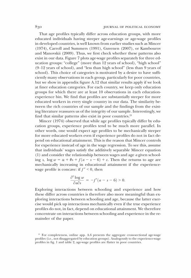
830 journal of political economy
That age profiles typically differ across education groups, with moreeducated individuals having steeper age-earnings or age-wage profilesin developed countries, is well known from earlier studies such as Mincer(1974), Carroll and Summers (1991), Guvenen (2007), or Kambourovand Manovskii (2009). Thus, we first check whether these patterns alsoexist in our data. Figure 7 plots age-wage profiles separately for three ed-ucation groups: “college” (more than 12 years of school), “high school”(9–12 years of school), and “less than high school” (less than 9 years ofschool). This choice of categories is motivated by a desire to have suffi-ciently many observations in each group, particularly for poor countries,but we show in appendix figure A.12 that similar results apply if we lookat finer education categories. For each country, we keep only educationgroups for which there are at least 10 observations in each education-experience bin. We find that profiles are substantially steeper for moreeducated workers in every single country in our data. The similarity be-tween the rich countries of our sample and the findings from the exist-ing literature reassures us of the integrity of our sample. Interestingly, wefind that similar patterns also exist in poor countries.21
Mincer (1974) observed that while age profiles typically differ by edu-cation groups, experience profiles tend to be much more parallel. Inother words, one would expect age profiles to be mechanically steeperfor more educated workers even if experience profiles do not in fact de-pend on educational attainment. This is the reason that Mincer controlsfor experience instead of age in the wage regression. To see this, assumethat individuals’ wages satisfy the additively separable Mincer equation(1) and consider the relationship between wages and age a given school-ing s, log w 5 a 1 vs 1 f ða 2 s 2 6Þ 1 ε. Then the returns to age aremechanically increasing in educational attainment if the experience-wage profile is concave: if f 00 < 0, then
∂2 log w
∂a∂s5 2f 00 a 2 s 2 6ð Þ > 0:
Exploring interactions between schooling and experience and howthese differ across countries is therefore also more meaningful than ex-ploring interactions between schooling and age, because the latter exer-cise would pick up interactions mechanically even if the true experienceprofiles do not, in fact, depend on educational attainment. We thereforeconcentrate on interactions between schooling and experience in the re-mainder of the paper.
21 For completeness, online app. A.6 presents the aggregate cross-sectional age-wageprofiles (i.e., not disaggregated by education groups). Analogously to the experience-wageprofiles in fig. 1 and table 2, age-wage profiles are flatter in poor countries.
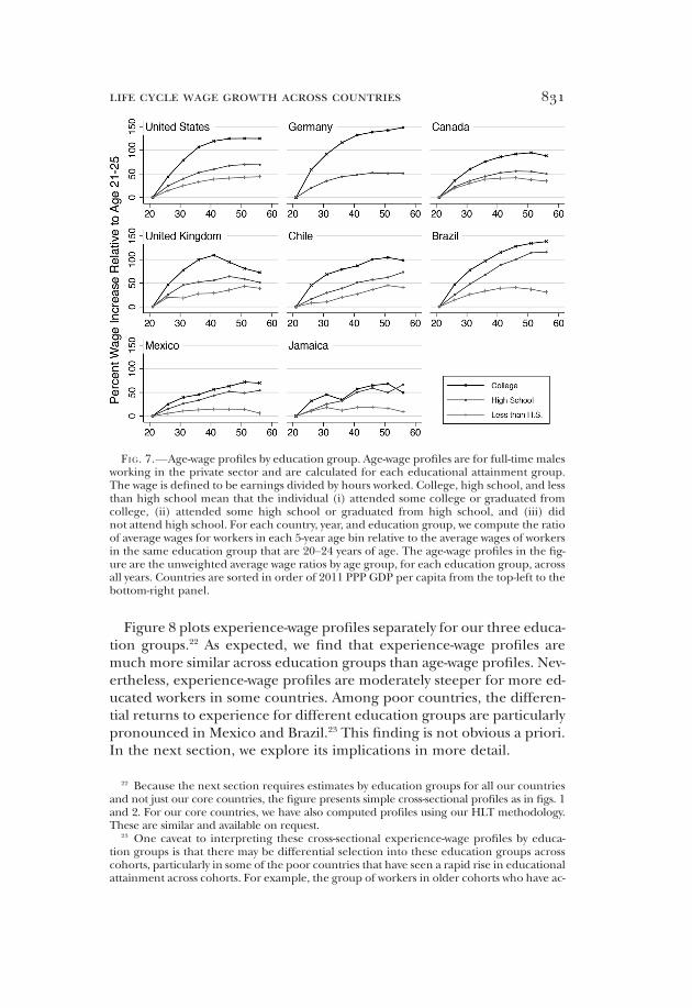
life cycle wage growth across countries 831
Figure 8 plots experience-wage profiles separately for our three educa-tion groups.22 As expected, we find that experience-wage profiles aremuch more similar across education groups than age-wage profiles. Nev-ertheless, experience-wage profiles are moderately steeper for more ed-ucated workers in some countries. Among poor countries, the differen-tial returns to experience for different education groups are particularlypronounced in Mexico and Brazil.23 This finding is not obvious a priori.In the next section, we explore its implications in more detail.
FIG. 7.—Age-wage profiles by education group. Age-wage profiles are for full-time malesworking in the private sector and are calculated for each educational attainment group.The wage is defined to be earnings divided by hours worked. College, high school, and lessthan high school mean that the individual (i) attended some college or graduated fromcollege, (ii) attended some high school or graduated from high school, and (iii) didnot attend high school. For each country, year, and education group, we compute the ratioof average wages for workers in each 5-year age bin relative to the average wages of workersin the same education group that are 20–24 years of age. The age-wage profiles in the fig-ure are the unweighted average wage ratios by age group, for each education group, acrossall years. Countries are sorted in order of 2011 PPP GDP per capita from the top-left to thebottom-right panel.
22 Because the next section requires estimates by education groups for all our countriesand not just our core countries, the figure presents simple cross-sectional profiles as in figs. 1and 2. For our core countries, we have also computed profiles using our HLT methodology.These are similar and available on request.
23 One caveat to interpreting these cross-sectional experience-wage profiles by educa-tion groups is that there may be differential selection into these education groups acrosscohorts, particularly in some of the poor countries that have seen a rapid rise in educationalattainment across cohorts. For example, the group of workers in older cohorts who have ac-
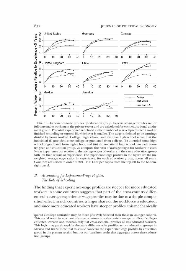
832 journal of political economy
B. Accounting for Experience-Wage Profiles:The Role of Schooling
The finding that experience-wage profiles are steeper for more educatedworkers in some countries suggests that part of the cross-country differ-ences in average experience-wage profiles may be due to a simple compo-sition effect: in rich countries, a larger share of the workforce is educated,and sincemore educated workers have steeper profiles, thismechanically
FIG. 8.—Experience-wage profiles by education group. Experience-wage profiles are forfull-time males working in the private sector and are calculated for each educational attain-ment group. Potential experience is defined as the number of years elapsed since a workerfinished schooling or turned 18, whichever is smaller. The wage is defined to be earningsdivided by hours worked. College, high school, and less than high school mean that theindividual (i) attended some college or graduated from college, (ii) attended some highschool or graduated from high school, and (iii) did not attend high school. For each coun-try, year, and education group, we compute the ratio of average wages for workers in each5-year experience bin relative to the average wages of workers in the same education groupwith less than 5 years of experience. The experience-wage profiles in the figure are the un-weighted average wage ratios by experience, for each education group, across all years.Countries are sorted in order of 2011 PPP GDP per capita from the top-left to the bottom-right panel.
quired a college education may be more positively selected than those in younger cohorts.This would result in mechanically steep cross-sectional experience-wage profiles of college-educated workers and mechanically flat cross-sectional profiles of less educated workers.This logic may partly explain the stark differences in profiles across education groups inMexico and Brazil. Note that this issue concerns the experience-wage profiles by educationgroup in the present section but not our baseline results that aggregate across these educa-tion groups.
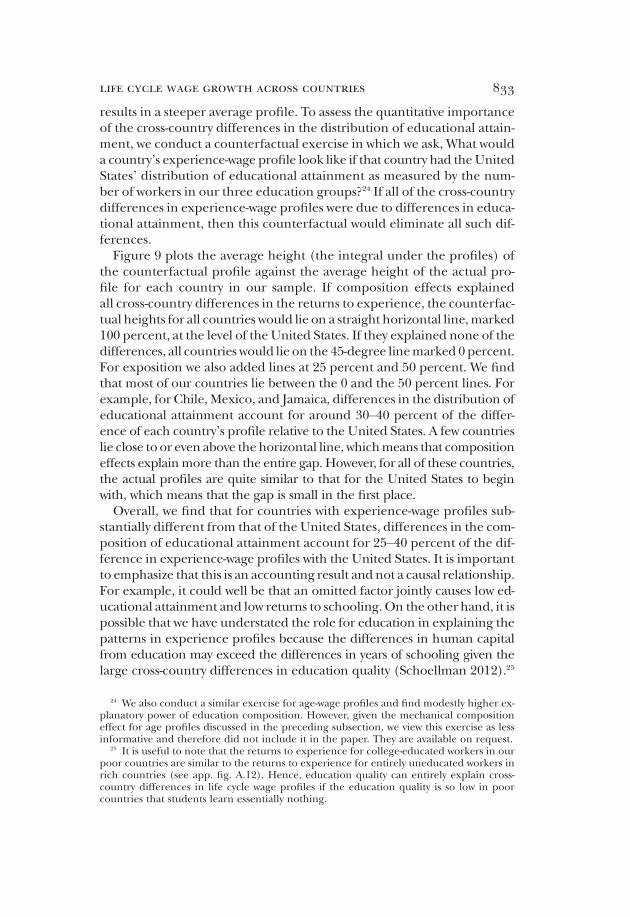
life cycle wage growth across countries 833
results in a steeper average profile. To assess the quantitative importanceof the cross-country differences in the distribution of educational attain-ment, we conduct a counterfactual exercise in which we ask, What woulda country’s experience-wage profile look like if that country had theUnitedStates’ distribution of educational attainment as measured by the num-ber of workers in our three education groups?24 If all of the cross-countrydifferences in experience-wage profiles were due to differences in educa-tional attainment, then this counterfactual would eliminate all such dif-ferences.Figure 9 plots the average height (the integral under the profiles) of
the counterfactual profile against the average height of the actual pro-file for each country in our sample. If composition effects explainedall cross-country differences in the returns to experience, the counterfac-tual heights for all countries would lie on a straight horizontal line,marked100 percent, at the level of the United States. If they explained none of thedifferences, all countries would lie on the 45-degree linemarked 0percent.For exposition we also added lines at 25 percent and 50 percent. We findthat most of our countries lie between the 0 and the 50 percent lines. Forexample, for Chile, Mexico, and Jamaica, differences in the distribution ofeducational attainment account for around 30–40 percent of the differ-ence of each country’s profile relative to the United States. A few countrieslie close toor even above the horizontal line, whichmeans that compositioneffects explainmore than the entire gap.However, for all of these countries,the actual profiles are quite similar to that for the United States to beginwith, which means that the gap is small in the first place.Overall, we find that for countries with experience-wage profiles sub-
stantially different from that of the United States, differences in the com-position of educational attainment account for 25–40 percent of the dif-ference in experience-wage profiles with the United States. It is importantto emphasize that this is an accounting result and not a causal relationship.For example, it could well be that an omitted factor jointly causes low ed-ucational attainment and low returns to schooling.On the otherhand, it ispossible that we have understated the role for education in explaining thepatterns in experience profiles because the differences in human capitalfrom education may exceed the differences in years of schooling given thelarge cross-country differences in education quality (Schoellman 2012).25
24 We also conduct a similar exercise for age-wage profiles and find modestly higher ex-planatory power of education composition. However, given the mechanical compositioneffect for age profiles discussed in the preceding subsection, we view this exercise as lessinformative and therefore did not include it in the paper. They are available on request.
25 It is useful to note that the returns to experience for college-educated workers in ourpoor countries are similar to the returns to experience for entirely uneducated workers inrich countries (see app. fig. A.12). Hence, education quality can entirely explain cross-country differences in life cycle wage profiles if the education quality is so low in poorcountries that students learn essentially nothing.
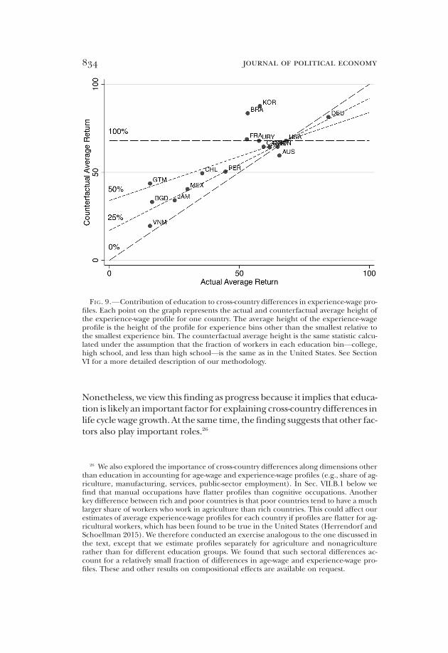
834 journal of political economy
Nonetheless, we view this finding as progress because it implies that educa-tion is likely an important factor for explaining cross-country differences inlife cycle wage growth.At the same time, thefinding suggests that other fac-tors also play important roles.26
FIG. 9.—Contribution of education to cross-country differences in experience-wage pro-files. Each point on the graph represents the actual and counterfactual average height ofthe experience-wage profile for one country. The average height of the experience-wageprofile is the height of the profile for experience bins other than the smallest relative tothe smallest experience bin. The counterfactual average height is the same statistic calcu-lated under the assumption that the fraction of workers in each education bin—college,high school, and less than high school—is the same as in the United States. See SectionVI for a more detailed description of our methodology.
26 We also explored the importance of cross-country differences along dimensions otherthan education in accounting for age-wage and experience-wage profiles (e.g., share of ag-riculture, manufacturing, services, public-sector employment). In Sec. VII.B.1 below wefind that manual occupations have flatter profiles than cognitive occupations. Anotherkey difference between rich and poor countries is that poor countries tend to have a muchlarger share of workers who work in agriculture than rich countries. This could affect ourestimates of average experience-wage profiles for each country if profiles are flatter for ag-ricultural workers, which has been found to be true in the United States (Herrendorf andSchoellman 2015). We therefore conducted an exercise analogous to the one discussed inthe text, except that we estimate profiles separately for agriculture and nonagriculturerather than for different education groups. We found that such sectoral differences ac-count for a relatively small fraction of differences in age-wage and experience-wage pro-files. These and other results on compositional effects are available on request.
life cycle wage growth across countries 835
VII. Potential Explanations
In this section, we discuss several potential explanations of lower life cy-cle wage growth in poor countries. We focus on three main candidatetheories suggested by the literature: human capital accumulation, searchand matching frictions, and long-term wage contracts. It is beyond thescope of this paper to conclusively rule in or rule out any particular the-ory. However, we can shed light on the likely relevance of theories bycomputing additional moments with our data. First, we compute life cy-cle wage profiles by broad occupation groups and find that manual oc-cupations have substantially flatter profiles than cognitive occupations.Second, we compute life cycle wage variance profiles, finding some evi-dence of U-shaped profiles, at least in the rich countries. Third, we lookat wage profiles for day laborers, who are not engaged in long-term wagecontracts, and find that, in the poor countries for which we have data,these are again flatter than in rich countries. Finally, we discuss the evi-dence from a companion study to this one that looks at experience-wageprofiles for immigrants to the United States. We find that these momentsare consistent with theories based on human capital or search frictionsand less supportive of models based on long-term contracts.
A. Candidate Mechanisms
1. Human Capital
There is a long tradition in economics that interprets experience-wageprofiles as reflecting human capital accumulation (Becker 1964). Underthis interpretation, our findings imply lower human capital accumula-tion over the life cycle in poor countries. The simplest version of this the-ory is that workers in poor countries use simpler technologies or engagein simpler tasks at work, for which there is less scope for learning. Onemay imagine that manual occupations, such as agricultural tasks, for ex-ample, have fewer possibilities for learning over the life cycle.27 It is wellknown that manual occupations are more common in poor countriesthan in rich countries.Another possibility is that workers in poor countries have fewer incen-
tives to accumulate human capital over their lifetimes. Manuelli andSeshadri (2014) propose a model of this type in which human capital ac-cumulation requires inputs of both goods and time, as in Ben-Porath
27 One way of capturing the idea that simpler technologies result in fewer learning op-portunities is as follows. Assume that the output of a firm is Leontief in the firm’s technol-ogy and the human capital of each of the workers it employs: y 5 oN
i51 minfA, hig, where ydenotes the firm’s output, A denotes its technology, and hi is the human capital of each ofits workers indexed by i 5 1, : : :,N . Since the human capital of a worker equals zero onceher human capital reaches A, no worker has an incentive to invest past this point.
836 journal of political economy
(1967). In theirmodel, low total factor productivity depresses the returnsto the accumulation of human capital by raising the price of physical in-puts to human capital production, thereby resulting in flat experience-wage profiles. Alternatively, extractive institutions in poor countries maydiscourage workers from investing in human capital, since their returnscan be arbitrarily expropriated (Bhattacharya, Guner, and Ventura 2013).This logic is consistent with recent evidence that higher taxation of laborincome in Europe can explain a substantial fraction of European-USdifferences in wage inequality and life cycle wage growth (Guvenen, Ku-ruscu, and Ozkan 2014).Another class of theories based on human capital accumulation fo-
cuses on learning through interactions with other individuals. For exam-ple, the models of Lucas (2009), Lucas and Moll (2014), and Perla andTonetti (2014) posit that human capital is accumulated through socialinteractions with others; all determinants of the frequency or qualityof such interactions are potential determinants of cross-country differ-ences in life cycle wage growth. As one example, de la Croix, Doepke,andMokyr (2016) argue that in the industrial revolution, the emergenceof institutions such as guilds allowed skills to be disseminated faster,which led to increased lifetime human capital accumulation and, hence,economic growth.
2. Search and Matching Frictions
Another candidate explanation for slow life cycle wage growth in poorcountries is search and matching frictions. If the labor market featuressearch frictions and match-specific productivity, slow life cycle wagegrowth in poor countries may partly reflect low labor market turnover.This could work through several mechanisms. Burdett (1978), Jovanovic(1984), Burdett and Mortensen (1998), and Bagger et al. (2014) empha-size on-the-job search as a theory of job shopping. If frictions to searchand matching lower the incentives or ability of workers to shop for jobs,they are less likely to climb the job ladder and will forgo some of the po-tential increase in labor productivity over the life cycle.28 Empirically,one would then expect to see workers in poor countries experiencingfewer job-to-job transitions and receiving smaller wage gains during suchtransitions.29
28 Burdett (1978, 219) puts it succinctly: “In the present study it has been assumed work-ers do not accumulate human capital while working. Older workers in the present studyreceive higher wage rates, on average, because they have obtained more job offers. Andthe more job offers a worker receives, the greater the probability a ‘high’ wage rate job willbe found.”
29 There is little work comparing such moments between rich and poor countries or re-gions. One exception is the study by Heise and Porzio (2015), who use matched employer-
life cycle wage growth across countries 837
Although these ideas have been applied to studying aggregate laborproductivity over the business cycle or across developed countries (Liseand Robin 2013; Postel-Vinay and Turon 2014), the large cross-countrydifferences in life cycle wage profiles suggest a nexploration. Alternatively,long-lasting frictionsmay prevent workers from sorting to the jobs that aremost suitable to their heterogeneous skills and tastes (Hsieh et al. 2013).Again, the implication would be that workers forgo labor productivity in-creases as they age.
3. Long-Term Contracts
Finally, if workers and firms form long-term contracts (e.g., Lazear 1979),wages may not equal workers’ marginal product of labor, and this maylead to cross-country differences in returns to experience.One version of these theories features back-loaded contracts, where
workers get less than their marginal products when young and morewhen they are older. This is the typical prediction of theories with moralhazard or limited commitment on the part of workers. These theorieshave the potential to explain our finding that experience-wage profilesare steeper in rich countries if long-term contracts are more prevalentin rich countries or they are equally prevalent but more back-loaded. Asecond version of these theories features front-loaded contracts, whereworkers get paid more than their marginal product when young and lesslater in the life cycle. Front-loading could arise, for example, becausefirms implicitly lend to financially constrained workers (Azariadis 1988;Bernhardt and Timmis 1990). To explain our findings, one would needa theory with more front-loading in poor countries. In summary, long-term contracts have the potential to explain flatter experience-wage pro-files in poor countries if wages are eithermore front-loaded in poor coun-tries or more back-loaded in rich countries or both.
B. Distinguishing between Mechanisms:Additional Moments
We now examine some additional moments in our data to attempt to dis-tinguish between potential mechanisms. We find several pieces of evi-dence that are consistent with human capital and search frictions con-tributing to our main findings and no obvious evidence that long-termcontracts play an important role. Distinguishing between human capital
employee data from Germany to compare wage dynamics in West Germany with those inthe considerably poorer East. They find that, when moving job to job, workers in the Eastexperience smaller wage gains than those in the richer West; i.e., they face a flatter job lad-der.

838 journal of political economy
and search is, in turn, more difficult for three reasons. First, our cross-sectional data do not allow us to construct moments typically thoughtto be informative about these two classes of theories, for example, wagechanges with job-to-job transitions. Second, search and human capitalaccumulation are difficult to tell apart even with high-quality panel dataor matched employer-employee data. One can think of workers in searchmodels accumulating “search capital” while employed that is destroyedupon job loss (Manning 2000), and at an abstract level, certain searchtheories may be observationally equivalent to theories of human capitalaccumulation. A number of existing studies assess the relative contribu-tion of human capital and job search in the United States and otherhigh-income countries (see, e.g., Topel and Ward 1992; Rubinstein andWeiss 2006; Altonji, Smith, andVidangos 2013; Bowlus andLiu 2013; Bag-ger et al. 2014). While these studies generally agree that both human cap-ital and search are important determinants of life cycle wage growth,there is considerable debate about the precise quantitative importanceof the two mechanisms, consistent with the idea that the two are hardto tell apart. Third, another difficulty is that there are likely nontrivial in-teractions between search and human capital (Bowlus and Liu 2013).With this in mind, we now present four pieces of evidence that makesome progress in distinguishing between potential explanations forcross-country differences in life cycle wage growth.
1. Experience-Wage Profiles by Occupation
We first explore differences in wage profiles by occupations. Most of oursamples report data on occupation. Although the occupational codingschemes vary by country, we are able to translate occupational codes intothe International Labour Office’s International Standard Classificationof Occupations (ISCO) at the one-digit level. We then aggregate theISCO one-digit occupational categories further to two broad categories:manual and cognitive. The reason we choose this split is that manual oc-cupations are relatively intensive in physical tasks, rather than mentalones, and may therefore have less scope for learning. If so, this may helpexplain our overall findings, since manual occupations are more com-mon in poor countries.In the data, we define manual occupations as elementary occupations,
agricultural workers, and plant/machine operators and assemblers (ISCOcodes 6, 8, and9). Cognitive occupations include legislators andmanagers,professionals, technicians, clerks, service and sales, and craftsmen (ISCOcodes 1–5 and 7).We exclude from this analysis workers withmissing occu-pations or those in the armed forces.For each country, we compute the life cycle wage profile of workers in
manual and cognitive occupations following our cross-sectional method

life cycle wage growth across countries 839
of Section III.30 In figure 10, we plot the resulting profiles by occupationfor our core countries. Two facts stand out. First, for all of our core coun-tries, the profiles are flatter formanual occupations than for cognitive occu-pations. Second, the difference is often substantial. For the average countryin our sample the return to 20–24 years of experience is 23 percentagepoints higher for workers in cognitive than in manual occupations.These differences potentially matter because of the sizable differences
in employment composition by country (plotted in app. fig. A.13). Richcountries have considerably more workers in cognitive occupations, atroughly 80 percent, while in poor countries the labor force is fairly evenlysplit. Formost countries, the employment composition across occupationschanges little inmagnitude over the life cycle, consistent with the idea thatmost workers will not systematically move from manual to cognitive workover the life cycle. The differences in life cycle wage growth across occupa-tions we find are particularly remarkable given our crude classification ofworkers into manual and cognitive occupations and given the likely possi-bility that a givenmanual occupation may vary in its manual and cognitiveintensity between rich and poor countries. We conjecture that more fine-grained data that allow for a less noisy proxy for occupations with differentlearning opportunities would likely result in even larger differences in em-ployment shares between rich and poor countries.As with education, we use a simple accounting exercise to quantify the
importance of occupation for aggregate life cycle wage profile differencesacross countries. As a reminder, the accounting exercise holds fixed eachcountry’s experience profiles by occupation and asks how much steeperthe country’s experience profile would be if it instead had the US em-ployment shares in cognitive and manual occupations. According to thisaccounting exercise, for most countries, the distribution of employmentacross occupations accounts for between 0 and 25 percent of the differ-ence of each country’s profile relative to the United States. Given the strik-ing differences in experience-wage profiles across occupations in figure 10,it is surprising that this counterfactual does not have larger predictivepower. Mechanically, this is true because with our crude occupational clas-sification, even in our poorest countries, the employment share in manualoccupations is only around 50 percent.
30 The reason for presenting the cross-sectional estimates rather than our HLTestimatesis that the accounting exercise below requires estimates by occupation groups for all ourcountries and not just our core countries. Moreover, the HLT methodology requires theassumption that there are no occupation transitions in the last 5 or 10 years of the life cycle,which could be more controversial than the analogous assumption about wage growth inour baseline HLTexercise. In any case, for our core countries, we have also computed pro-files by occupation using our HLT methodology. These are similar to the cross-sectionalestimates and are available on request.
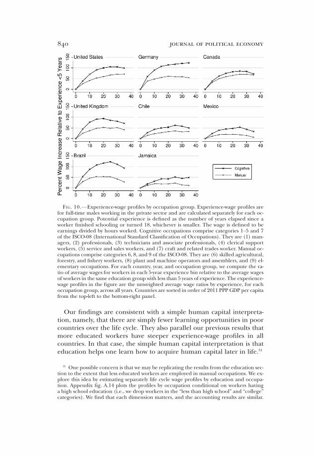
840 journal of political economy
Our findings are consistent with a simple human capital interpreta-tion, namely, that there are simply fewer learning opportunities in poorcountries over the life cycle. They also parallel our previous results thatmore educated workers have steeper experience-wage profiles in allcountries. In that case, the simple human capital interpretation is thateducation helps one learn how to acquire human capital later in life.31
FIG. 10.—Experience-wage profiles by occupation group. Experience-wage profiles arefor full-time males working in the private sector and are calculated separately for each oc-cupation group. Potential experience is defined as the number of years elapsed since aworker finished schooling or turned 18, whichever is smaller. The wage is defined to beearnings divided by hours worked. Cognitive occupations comprise categories 1–5 and 7of the ISCO-08 (International Standard Classification of Occupations). They are (1) man-agers, (2) professionals, (3) technicians and associate professionals, (4) clerical supportworkers, (5) service and sales workers, and (7) craft and related trades worker. Manual oc-cupations comprise categories 6, 8, and 9 of the ISCO-08. They are (6) skilled agricultural,forestry, and fishery workers, (8) plant and machine operators and assemblers, and (9) el-ementary occupations. For each country, year, and occupation group, we compute the ra-tio of average wages for workers in each 5-year experience bin relative to the average wagesof workers in the same education group with less than 5 years of experience. The experience-wage profiles in the figure are the unweighted average wage ratios by experience, for eachoccupation group, across all years. Countries are sorted in order of 2011 PPP GDP per capitafrom the top-left to the bottom-right panel.
31 One possible concern is that we may be replicating the results from the education sec-tion to the extent that less educated workers are employed in manual occupations. We ex-plore this idea by estimating separately life cycle wage profiles by education and occupa-tion. Appendix fig. A.14 plots the profiles by occupation conditional on workers havinga high school education (i.e., we drop workers in the “less than high school” and “college”categories). We find that each dimension matters, and the accounting results are similar.
life cycle wage growth across countries 841
2. Experience-Wage Profiles of Day Laborers
We next explore the importance of labor market contracts for our pat-terns. We note first that theories of long-term contracting all refer tothe returns to tenure (experience at a specific firm) rather than the re-turn to lifetime potential experience. Thus, long-term contracts are un-likely to have large quantitative effects on experience-wage profiles unlessaverage worker tenure is reasonably long. The limited data on worker ten-ure do not support this: for example, in theUnited States, themedian ten-ure is 4.6 years (Bureau of Labor Statistics 2012), and for Brazil, Chile,Gua-temala, Jamaica, Peru, and Uruguay, it ranges between 1.5 and 5.5 years(Interamerican Development Bank 2016).32
To provide additional evidence on this point, we study the life cyclewage profiles of workers employed without long-term contracts. The ra-tionale is that these profiles speak directly to the question of whether ourpatterns are likely to be explained by contractual arrangements betweenworkers and firms that introduce a wedge between life cycle wage andlife cycle productivity profiles. We provide such evidence for three coun-tries for which we can identify workers who are unlikely to be on long-term contracts. For India andMexico, we can identify a subset of workerswho are daily workers: those whose employer varies on a day-to-day basis.Clearly, these workers’ profiles are not driven by employer-specific con-tracting. For the United States, we draw on the Current Population Sur-vey (King et al. 2010), where we can identify workers who work part-timeand are not interested in working full-time even if it were available. Theseworkers report other commitments (home, family, and so on) that makefull-time work undesirable. Since these workers apparently value the flex-ibility and lack of commitment that come with short-term work arrange-ments, our interpretation is that they are also unlikely to be taking part inlong-term contracts.Appendix figure A.15 presents the experience-wage profiles for work-
ers on short-term contracts and the rest of the workforce in these threecountries. Recall from above that long-term contracts can explain flatterexperience-wage profiles in poor countries in two scenarios. The firstscenario is that wages are more front-loaded in poor countries. In thiscase we would expect day laborers in poor countries to have steeper pro-files than the rest of the workforce. The second scenario is that wages aremore back-loaded in rich countries. In this case, we would expect day la-borers in rich countries to have flatter profiles. We find no evidence ofeither of these scenarios. In India and the United States the two sets
32 The Interamerican Development Bank (2016) provides estimates only for Central andSouth American countries, and we are not aware of corresponding data for other countriesin our sample. The numbers for Brazil, Chile, Guatemala, Jamaica, Peru, and Uruguay aremedian tenure for the most recent year in which these data are available.

842 journal of political economy
of profiles are quite similar, and in Mexico the day laborers have flatterprofiles than other workers. An obvious caveat to this exercise is that daylaborers are likely a selected group of workers who differ from the rest ofthe workforce in a number of other characteristics, for example, theirskills. Nevertheless, the comparison of day laborers to other workers to-gether with the relatively short job tenure of the typical worker in bothrich and poor countries suggests that long-term contracts are unlikely toexplain our cross-country patterns.
3. Variance Profiles
Thus far, we have focused on mean wages by experience. Now we turnour attention to the variance of wages by experience to see if they canprovide any additional information. Both human capital and searchmodels make a wide variety of predictions for how the variance of wagesmight evolve over the life cycle. Hence, these predictions are useful fordiscriminating among specific human capital theories or among searchtheories, but not between the two.For human capital models, the key determinant of the shape of vari-
ance profiles is the correlation between learning ability and initial hu-man capital (Huggett et al. 2011). Intuitively, individuals with higherlearning ability endogenously choose to invest more at the beginningof the life cycle. These choices lead them to have steeper wage profilesthan individuals with low learning ability. The level of initial human cap-ital mostly affects the intercept of the profile. Hence, if the two are weaklycorrelated, the model predicts that high–learning ability individualshave lower levels but steeper slopes of wages than their low–learning abil-ity counterparts. Therefore, profiles cross at some point, implying a U-shaped pattern for the variance of wages over the life cycle (Mincer 1974;Rubinstein andWeiss 2006). On the other hand, if the two are sufficientlystrongly positively correlated, then high–learning ability individuals willhave higher levels and steeper slopes of wages, implying that the varianceof wages rises continuously over the life cycle.Among search theories, we focus on theories of on-the-job search be-
cause these have implications for life cycle wage profiles. Hornstein,Krusell, and Violante (2011) show that some recent theories of on-the-job search have the potential to generate realistic levels of wage disper-sion. The implications for the shape of variance profiles over the life cy-cle are less clear. Among existing theories, the study by Bagger et al. (2014)stands out for making quantitative predictions about the life cycle profileof wage dispersion, finding that it rises at a decreasing rate.33 The key
33 Burdett, Carrillo-Tudela, and Coles (2011) also formulate a model with life cycle pat-terns of dispersion, but they do not calibrate or estimate the model to provide a full de-scription of what the profile might look like.
life cycle wage growth across countries 843
mechanism is a rise in the heterogeneity of firms that workers are matchedwith over the life cycle. In contrast, Manning (2000) presents a simplemodel of on-the-job search that generates a U-shaped life cycle varianceprofile.To compute variances over the life cycle, we take the variance of log
wages in each experience bin, by the three education groups discussedabove. We then take the weighted average log wage variance across expe-rience bins, where each education group is weighted by its share amongall workers. Figure 11 plots profiles for the variance of the logarithm ofwages across countries. The empirical results generally follow one of twopatterns. In four of the five richest countries (top-left quadrant) as wellas in South Korea and Jamaica, variance profiles follow a U shape: declin-ing at the beginning of the life cycle and then rising toward the end. In theremaining countries (the United States and most poorer countries), theprofiles are generally rising throughout the life cycle.34 In summary, the ev-idence on variance profiles is mixed and appears consistent with differ-ent versions of both human capital and search theories. For both classesof theories, our empirical results imply restrictions on the range of plau-sible parameterizations that will be consistent with the data in differentcountries. This is an interesting avenue for future research.35
4. Evidence from Immigrants to the United States
In a companion paper (Lagakos et al. 2016), we study how wages in theUnited States vary for immigrant workers of different experience levels.We document that, for immigrants from rich countries, more experi-enced immigrants tend to earn substantially more than less experiencedimmigrants. In contrast, for immigrants from poor countries, more ex-perienced immigrants tend to earn only somewhat more than the lessexperienced. We show that this is true for new immigrants, who earnedall their experience abroad, as well as for all immigrants when we controlfor the amount of US work experience.
34 In some countries, the variance profiles are mildly declining at the end of the life cy-cle, a pattern that could be interpreted as an inverse U shape.
35 In Ben-Porath-type models, one form of investment in human capital accumulationmay be reflected in part-time work and low hours worked more broadly. To investigate thispossibility, in online app. A.7 we relax the restriction to only full-time workers that we havemade so far and examine hours and earnings profiles over the life cycle in this larger sam-ple. We find that in rich countries, hours rise steeply early on in the life cycle, largely re-flecting movements from part-time into full-time work. These cross-country patterns areconsistent with theories of human capital accumulation, in particular, the prediction thatworkers in rich countries initially invest a lot of time in human capital accumulation, andtherefore work little, but then increase their time working over their life cycle. The fact thatpoor countries generally do not see such hours increases is consistent with the predictionof less investment early in the life cycle. We also examine variance profiles in the largersample including both part-time and full-time workers and find stronger evidence of aU shape (perhaps unsurprisingly given the evidence on hours profiles).
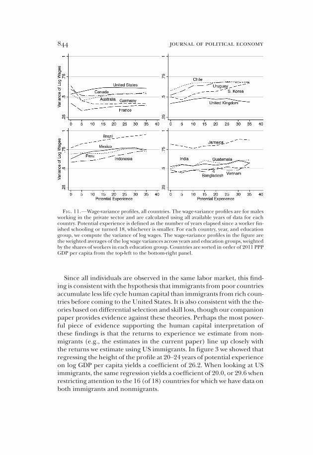
844 journal of political economy
Since all individuals are observed in the same labor market, this find-ing is consistent with the hypothesis that immigrants from poor countriesaccumulate less life cycle human capital than immigrants from rich coun-tries before coming to the United States. It is also consistent with the the-ories based ondifferential selection and skill loss, though our companionpaper provides evidence against these theories. Perhaps the most power-ful piece of evidence supporting the human capital interpretation ofthese findings is that the returns to experience we estimate from non-migrants (e.g., the estimates in the current paper) line up closely withthe returns we estimate using US immigrants. In figure 3 we showed thatregressing the height of the profile at 20–24 years of potential experienceon log GDP per capita yields a coefficient of 26.2. When looking at USimmigrants, the same regression yields a coefficient of 20.0, or 29.6 whenrestricting attention to the 16 (of 18) countries for which we have data onboth immigrants and nonmigrants.
FIG. 11.—Wage-variance profiles, all countries. The wage-variance profiles are for malesworking in the private sector and are calculated using all available years of data for eachcountry. Potential experience is defined as the number of years elapsed since a worker fin-ished schooling or turned 18, whichever is smaller. For each country, year, and educationgroup, we compute the variance of log wages. The wage-variance profiles in the figure arethe weighted averages of the log wage variances across years and education groups, weightedby the shares of workers in each education group. Countries are sorted in order of 2011 PPPGDP per capita from the top-left to the bottom-right panel.

life cycle wage growth across countries 845
5. Summary of Evidence
In summary, the four pieces of evidence we presented in this section sug-gest that long-term contracts are unlikely to be an important driver ofcross-country differences in life cycle wage growth. In contrast, both hu-man capital and search appear consistent with the moments we have pre-sented here. A particularly simple explanation for slow life cycle wagegrowth in poor countries is that workers in poor countriesmay simply havefewer opportunities for learning because of the nature of the occupationsor tasks they perform, consistent with the evidence on experience-wageprofiles across occupations we presented above. At the same time and asnoted in the beginning of this section, it is generally hard to tell apart hu-man capital and search as drivers of life cycle wage growth, and as such,more severe labor market frictions are an equally promising candidate ex-planation for flat experience-wage profiles in poor countries.
VIII. Conclusion
This paper documents that experience-wage profiles are steeper in richcountries than inpoor countries. In the rich countries, thewages of themostexperienced workers are, on average, almost 100 percent larger than thewages of the least experienced workers. In contrast, in the poor countries,the wages of the most experienced workers are only around 50 percentlarger than the wages of the least experienced workers.We find that some,but not all, of this pattern is accounted for by differences in education lev-els across countries, with more educated workers having steeper profiles.While it is difficult to provide a definitive explanation of our findings,
several additional moments of our data support human capital or searchfrictions as promising explanations. Providing a more definitive explana-tion for cross-country differences in life cycle wage growth is an importanttask for future research. In particular, doing so could help account forcross-country income differences. Earlier studies in this literature foundno relationship between returns to experience and GDP per capita(Psacharopoulos 1994; Bils and Klenow 2000) and concluded that it wassafe to ignore any cross-country human capital differences arising throughexperience rather than schooling. Recent work by Manuelli and Seshadri(2014) predicts that workers in rich countries accumulate more humancapital over the life cycle as well, and our evidence offers support for thisidea. If true, the importance of human capital in accounting for incomedifferences is substantially higher than previously concluded.36
36 Any development accounting exercise along these lines would need to be careful todistinguish between two different forms of human capital accumulation with potentiallydifferent quantitative implications: on-the-job training as in Ben-Porath (1967) and learn-

846 journal of political economy
Turning to the implications of a search-based explanation of flat experi-ence profiles in poor countries, the macro-development literature gener-ally assumes competitive labor markets. The main exceptions are papersthat focus on distortions to the allocation across sectors or locations, whichgenerate misallocations of labor (Caselli 2005; Restuccia, Yang, and Zhu2008; Gollin, Lagakos, and Waugh 2014). Viewed through the lens of asearch andmatchingmodel, our findings suggest that it may be time to in-corporate analogous frictions to on-the-job search or job choice that gen-erate misallocation of labor over the life cycle. Explorations along theselineswould be particularly interesting given that low labormarket turnoverin poor countries could have implications for a number of important issuesbesides aggregate productivity. For example, low turnover could hampermobility if poor workers escapingpoverty involves an element of “job shop-ping.”
References
Aguiar, Mark, and Erik Hurst. 2013. “Deconstructing Life Cycle Expenditure.”J.P.E. 121 (3): 437–92.
Altonji, Joseph G., Anthony A. Smith Jr., and Ivan Vidangos. 2013. “ModelingEarnings Dynamics.” Econometrica 81 (4): 1395–1454.
Azariadis, Costas. 1988. “Human Capital and Self-Enforcing Contracts.” Scandi-navian J. Econ. 90 (4): 507–28.
Bagger, Jesper, Francois Fontaine, Fabien Postel-Vinay, and Jean-Marc Robin.2014. “Tenure, Experience, Human Capital, and Wages: A Tractable Equilib-rium Search Model of Wage Dynamics.” A.E.R. 104 ( June): 1551–96.
Becker, Gary S. 1964. Human Capital: A Theoretical and Empirical Analysis, with Spe-cial Reference to Education. Chicago: Univ. Chicago Press.
Ben-Porath, Yoram. 1967. “The Production of Human Capital and the Life Cycleof Earnings.” J.P.E. 75 (4): 352–65.
Bernhardt, Dan, and Gerald C. Timmis. 1990. “Multiperiod Wage Contracts andProductivity Profiles.” J. Labor Econ. 8 (October): 529–63.
Bhattacharya, Dhritman, Nezih Guner, and Gustavo Ventura. 2013. “Distortions,Endogenous Managerial Skills and Productivity Differences.” Rev. Econ. Dy-namics 16 ( January): 11–25.
Bils, Mark, and Peter J. Klenow. 2000. “Does Schooling Cause Growth?” A.E.R. 90(December): 1160–83.
Bowlus, Audra J., and Huju Liu. 2013. “The Contributions of Search and HumanCapital to Earnings Growth over the Life Cycle.” European Econ. Rev. 64:305–31.
Bowlus, Audra J., and Chris Robinson. 2012. “Human Capital Prices, Productiv-ity, and Growth.” A.E.R. 102 (7): 3483–3515.
ing by doing. Through the lens of models of on-the-job training, the steep wage growth inearly years of the life cycle in rich countries may partly reflect a declining time investmentin human capital accumulation, so that the underlying human capital profile is flatter thanthe observed wage profile. Therefore, cross-country differences in life cycle human capitalwould be smaller than those implied by simple learning-by-doing models in which a work-er’s wage is proportional to her human capital.
life cycle wage growth across countries 847
Burdett, Kenneth. 1978. “A Theory of Employee Job Search and Quit Rates.”A.E.R. 68 (1): 212–20.
Burdett, Kenneth, Carlos Carrillo-Tudela, and Melvyn G. Coles. 2011. “HumanCapital Accumulation and Labor Market Equilibrium.” Internat. Econ. Rev. 52(August): 657–77.
Burdett, Kenneth, and Dale T. Mortensen. 1998. “Wage Differentials, EmployerSize, and Unemployment.” Internat. Econ. Rev. 39 (May): 257–73.
Bureau of Labor Statistics. 2012. “Employee Tenure Summary.”Washington, DC:Bur. Labor Statis.
Cagan, Phillip. 1973. “Measuring Quality Changes and the Purchasing Power ofMoney: An Exploratory Study of Automobiles.” In Price Indexes and QualityChange, edited by Zvi Griliches. Cambridge, MA: Harvard Univ. Press.
Carroll, Christopher D., and Lawrence H. Summers. 1991. “ConsumptionGrowth Parallels Income Growth: Some New Evidence.” In National Savingand Economic Performance, edited by B. Douglas Bernheim and John B. Shoven,305–43. Chicago: Univ. Chicago Press.
Caselli, Francesco. 2005. “Accounting for Cross-Country Income Differences.” InHandbook of Economic Growth, edited by P. Aghion and S. Durlauf, 679–741. Am-sterdam: Elsevier.
Deaton, Angus. 1997. The Analysis of Household Surveys: A Microeconometric Ap-proach to Development Policy. Washington, DC: World Bank.
de la Croix, David, Matthias Doepke, and Joel Mokyr. 2016. “Clans, Guilds, andMarkets: Apprenticeship Institutions and Growth in the Pre-industrial Econ-omy.” Working paper, Northwestern Univ.
Duflo, Esther. 2001. “Schooling and Labor Market Consequences of School Con-struction in Indonesia: Evidence from an Unusual Policy Experiment.” A.E.R.91 (4): 795–813.
Gollin, Douglas. 2002. “Getting Income Shares Right.” J.P.E. 110 (April): 458–74.Gollin, Douglas, David Lagakos, and Michael E. Waugh. 2014. “The Agricultural
Productivity Gap.” Q.J.E. 129 (2): 939–93.Gould, William, and Finis Welch. 1976. “Imputing Labor Market Experience.”
Manuscript, Rand Corp., Santa Monica, CA.Guvenen, Fatih. 2007. “Learning Your Earning: Are Labor Income Shocks Really
Very Persistent?” A.E.R. 97 ( June): 687–712.Guvenen, Fatih, Fatih Karahan, Serdar Ozkan, and Jae Song. 2014. “What Do
Data onMillions of U.S. Workers Reveal about Life-Cycle Earnings Risk?”Man-uscript, Fed. Reserve Bank Minneapolis.
Guvenen, Fatih, Burhanettin Kuruscu, and Serdar Ozkan. 2014. “Taxation of Hu-man Capital and Wage Inequality: A Cross-Country Analysis.” Rev. Econ. Studies81 (2): 818–50.
Hall, Robert E. 1968. “Technical Change and Capital from the Point of View ofthe Dual.” Rev. Econ. Studies 35 (1): 35–46.
Hanoch, Giora. 1967. “An Economic Analysis of Earnings and Schooling.” J. Hu-man Resources 2 (3): 310–29.
Heckman, James, Lance Lochner, and Christopher Taber. 1998. “Explaining Ris-ingWage Inequality: Explanations with a Dynamic General EquilibriumModelof Labor Earnings with Heterogeneous Agents.” Rev. Econ. Dynamics 1 ( Janu-ary): 1–58.
Heckman, James, and Richard Robb. 1985. “Using Longitudinal Data to Esti-mate Age, Period and Cohort Effects in Earnings Equations.” In Cohort Analysisin Social Research, edited by William M. Mason and Stephen E. Fienberg, 137–50. New York: Springer.

848 journal of political economy
Heise, Sebastian, and Tommaso Porzio. 2015. “Unemployment Risk and Flat JobLadders: Lessons from the German Reunification.”Working paper, Yale Univ.
Herrendorf, Berthold, and Todd Schoellman. 2015. “Why Is Measured Produc-tivity So Low in Agriculture?” Rev. Econ. Dynamics 18 (4): 1003–22.
Hornstein, Andreas, Per Krusell, and Giovanni L. Violante. 2011. “FrictionalWage Dispersion in Search Models: A Quantitative Assessment.” A.E.R. 101(December): 2873–98.
Hsieh, Chang-Tai, Erik Hurst, Charles I. Jones, and Peter J. Klenow. 2013. “TheAllocation of Talent and U.S. Economic Growth.” Working Paper no. 18693( January), NBER, Cambridge, MA.
Huggett, Mark, Gustavo Ventura, and Amir Yaron. 2011. “Sources of Lifetime In-equality.” A.E.R. 101 (7): 2923–54.
Hurst, Erik, Geng Li, and Ben Pugsley. 2014. “Are Household Surveys Like TaxForms? Evidence from Income Underreporting of the Self Employed.” Rev.Econ. and Statis. 96 (1): 19–33.
Inter-American Development Bank. 2016. Harmonized Household Survey DataBases of Latin America and the Caribbean—Sociómetro-BID. Washington, DC:Inter-American Development Bank.
Jovanovic, Boyan. 1984. “Matching, Turnover, and Unemployment.” J.P.E. 92 (1):972–90.
Kambourov, Gueorgui, and Iourii Manovskii. 2009. “Accounting for the ChangingLife-Cycle Profile of Earnings.” Working paper, Dept. Econ., Univ. Pennsylvania.
King,Miriam, et al. 2010. Integrated Public UseMicrodata Series, Current Population Sur-vey: Version 3.0 [machine-readable database]. Minneapolis: Univ. Minnesota.
Klenow, Pete, and Andres Rodriguez-Clare. 1997. “The Neoclassical Revival inGrowth Economics: Has It Gone Too Far?” In NBER Macroeconomics Annual,vol. 12, edited by Ben S. Bernanke and Julio J. Rotemberg, 73–114. Cam-bridge, MA: MIT Press.
Lagakos, David, Benjamin Moll, Tommaso Porzio, Nancy Qian, and ToddSchoellman. 2012. “Experience Matters: Human Capital and Development Ac-counting.” Working Paper no. 18602 (December), NBER, Cambridge, MA.
———. 2016. “Lifecycle Human Capital Accumulation across Countries: Lessonsfrom U.S. Immigrants.” Working Paper no. 21914 ( January), NBER, Cam-bridge, MA.
Lazear, Edward P. 1979. “Why Is There Mandatory Retirement?” J.P.E. 87 (De-cember): 1261–84.
Lehmann, Erich Leo, and Joseph P. Romano. 2005. Testing Statistical Hypotheses.New York: Springer.
Lemieux, Thomas. 2006. “TheMincer Equation Thirty Years after Schooling, Ex-perience, and Earnings.” In Jacob Mincer: A Pioneer of Modern Labor Economics,edited by S. Grossbard-Schechtman, 127–45. New York: Springer.
Lise, Jeremy, and Jean-Marc Robin. 2013. “The Macro-Dynamics of Sorting be-tween Workers and Firms.” Working Paper no. W13/22 (August), Inst. FiscalStudies, London.
Lucas, Robert E. 2009. “Ideas and Growth.” Economica 76 (301): 1–19.Lucas, Robert E., and Benjamin Moll. 2014. “Knowledge Growth and the Alloca-
tion of Time.” J.P.E. 122 (1): 1–51.Manning, Alan. 2000. “Movin’ on Up: Interpreting the Earnings-Experience Pro-
file.” Bull. Econ. Res. 52 (October): 261–95.Manuelli, Rodolfo E., and Ananth Seshadri. 2014. “Human Capital and the
Wealth of Nations.” A.E.R. 104 (9): 2736–62.
life cycle wage growth across countries 849
McKenzie, David J. 2006. “Disentangling Age, Cohort and Time Effects in the Ad-ditive Model.” Oxford Bull. Econ. and Statis. 68 (4): 473–95.
Mincer, Jacob A. 1974. Schooling, Experience, and Earnings. New York: ColumbiaUniv. Press (for NBER).
Minnesota Population Center. 2011. Integrated Public Use Microdata Series, Interna-tional: Version 6.1 [machine-readable database]. Minneapolis: Univ. Minnesota.
Murphy, Kevin M., and Finis Welch. 1990. “Empirical Age-Earnings Profiles.” J.Labor Econ. 8 (April): 202–29.
Perla, Jesse, and Christopher Tonetti. 2014. “Equilibrium Imitation and Growth.”J.P.E. 122 (1): 52–76.
Postel-Vinay, Fabien, and Hélène Turon. 2014. “The Impact of Firing Restric-tions on Labour Market Equilibrium in the Presence of On-the-Job Search.”Econ. J. 124 (575): 31–61.
Psacharopoulos, George. 1994. “Returns to Investment in Education: A GlobalUpdate.” World Development 22 (9): 1325–43.
Restuccia, Diego, Dennis Tao Yang, and Xiaodong Zhu. 2008. “Agriculture andAggregate Productivity: A Quantitative Cross-Country Analysis.” J. MonetaryEcon. 55:234–50.
Rubinstein, Yona, and Yoram Weiss. 2006. “Post Schooling Wage Growth: Invest-ment, Search and Learning.” In Handbook of the Economics of Education, vol. 1,edited by Eric Hanushek and Finis Welch, 1–67. Amsterdam: Elsevier.
Salthouse, Timothy A. 2003. “Interrelations of Aging, Knowledge, and CognitivePerformance.” In Understanding Human Development: Dialogues with Lifespan Psy-chology, edited by Ursula M. Staudinger and Ulman Lindenberger, 265–87.New York: Springer.
———. 2013. “Within-Cohort Age-Related Differences in Cognitive Function-ing.” Psychological Sci. 24 (2): 123–30.
Schoellman, Todd. 2012. “Education Quality and Development Accounting.”Rev. Econ. Studies 3 (March): 133–75.
Schulhofer-Wohl, Sam. 2013. “The Age-Time-Cohort Problem and the Identifi-cation of Structural Parameters in Life-Cycle Models.” Manuscript, Fed. Re-serve Bank Minneapolis.
Smith, James P., and Finis Welch. 1978. “Race Differences in Earnings: A Surveyand New Evidence.” Tech. Report no. R-2295-NSF, Rand Corp., Santa Mon-ica, CA.
Tanaka, Hirofumi, and Douglas R. Seals. 2008. “Endurance Exercise Perfor-mance in Masters Athletes: Age-Associated Changes and Underlying Physio-logical Mechanisms.” J. Physiology 586 (1): 55–63.
Todaro, Michael P., and Stephen C. Smith. 2012. Economic Development. 11th ed.Boston: Addison-Wesley.
Topel, Robert H., and Michael P. Ward. 1992. “Job Mobility and the Careers ofYoung Men.” Q.J.E. 107 (May): 439–79.
Welch, Finis. 1979. “Effects of Cohort Size on Earnings: The Baby Boom Babies’Financial Bust.” J.P.E. 87, no. 5, pt. 2 (October): S65–S97.