DI

SC

US

SI

ON

P

AP

ER

S

ER

IE

S

Forschungsinstitut zur Zukunft der ArbeitInstitute for the Study of Labor

Wage Work for Women:The Menstrual Cycle and the Power of Water

IZA DP No. 4776

February 2010

Yasheng MaimaitiW. S. Siebert

Wage Work for Women: The Menstrual

Cycle and the Power of Water

Yasheng Maimaiti University of Birmingham

W. S. Siebert

University of Birmingham and IZA

Discussion Paper No. 4776 February 2010

IZA

P.O. Box 7240 53072 Bonn

Germany

Phone: +49-228-3894-0 Fax: +49-228-3894-180

E-mail: iza@iza.org

Any opinions expressed here are those of the author(s) and not those of IZA. Research published in this series may include views on policy, but the institute itself takes no institutional policy positions. The Institute for the Study of Labor (IZA) in Bonn is a local and virtual international research center and a place of communication between science, politics and business. IZA is an independent nonprofit organization supported by Deutsche Post Foundation. The center is associated with the University of Bonn and offers a stimulating research environment through its international network, workshops and conferences, data service, project support, research visits and doctoral program. IZA engages in (i) original and internationally competitive research in all fields of labor economics, (ii) development of policy concepts, and (iii) dissemination of research results and concepts to the interested public. IZA Discussion Papers often represent preliminary work and are circulated to encourage discussion. Citation of such a paper should account for its provisional character. A revised version may be available directly from the author.

IZA Discussion Paper No. 4776 February 2010

ABSTRACT

Wage Work for Women:

The Menstrual Cycle and the Power of Water We hypothesise that women’s participation in wage (off-farm) work is reduced when their greater water needs due to the menstrual cycle are not met because their household has poor access to water. For testing, we use the data from rural villages in China. Controlling for village fixed effects, poor access to water is found to decrease the probability of wage work participation of affected (pre-menopause) women by about 10 percentage points, a large effect. As expected, there is no adverse causal impact of poor household access to water for women post-menopause, or for men, ceteris paribus.

NON-TECHNICAL SUMMARY

In this study, we investigate the impact of poor access to water on women’s wage work participation in rural China. This study hypothesises that women pre-menopause face higher costs of participation and achieve lower productivity when access to water is poor (holding other things equal), and therefore have lower rate of wage work participation. We use the China Health and Nutrition Survey dataset for 1993 to test the hypothesis. In this dataset, about half of the respondents do not have access to improved water, and also a large number of respondents are not involved in any type of wage work. Most importantly, there is specific information about women’s menopause status. We use both regression analysis and Propensity Score Matching methods to test the hypothesis. Both approaches yield supportive results. Women pre-menopause are found to be especially affected by poor access to water, that is, their probability of participating in wage work is about 10 percentage points lower than their peers with good access to water controlling for other confounding factors. For men, and for women post-menopause, poor access to water per se has no causal impact on wage work participation. Therefore, a major benefit of policies to improve water supplies may not be the obvious household or industrial benefit, but rather an unseen benefit, the improvement in the working position of women. While much of these benefits have already been gained in China which has made good progress in raising access to water, the results should be relevant to other areas of the developing world. JEL Classification: J16, J21, O15 Keywords: wage work, women, menopause, water engineering, rural development, China Corresponding author: W. S. Siebert Birmingham Business School University House Edgbaston Birmingham B15 2TT United Kingdom E-mail: w.s.siebert@bham.ac.uk

2

1. Introduction

In the developing world, women’s participation in wage work (off-farm work) fallswell behind that of men, reducing women’s income (Zhang et al, 2002, 2004), andwomen’s reproductive health (Stewart et al 2004, Wang 2007). There are alsoimportant implications for society and democracy. Lack of employment outside thehome reduces women’s participation in the political system (Burns, 1997; Chhibber,2002), which feeds back into less concern for women’s education, and perhaps a lesssecure democracy given the link (Glaeser et al, 2007) between education anddemocracy. Indeed, increasing the proportion of women in wage employment in thenon-agricultural sector is now one of the United Nation’s millennium developmentgoals to empower women (UN, 2009).

This paper starts from the observation that women fall behind particularlywhen the household has poor access to water. Figure 1 demonstrates this fact, using across-country dataset. Moreover, menstrual health problems are reported to be morepronounced for women with poor hygiene facilities (Ahmed and Yesmin, 2008) orwho experience stress (Deuster et al., 1999) which can be linked to poor access towater. Building on these observations, we hypothesise that where there is a lack of tapwater for women to wash during the menstrual cycle, they will find it more difficult tobe hired for, and succeed in, wage work. Water engineering might therefore have arole in advancing not only women's education and health, but also their incomes, andultimately their wider participation in society.

Variables relating to the menstrual cycle, and to water supply, have onlyrecently begun appearing in economic analysis. In studies of education, following thedevelopment literature (e.g., Bharadwaj and Patkar, 2004) the onset of menstruation(menarche) is increasingly seen as playing a role in explaining rural girls’ lowschooling attainment (but for contrary evidence see Oster and Thornton, 2008).Possible avenues are that menarche pushes elder sisters into early marriage (Field andArbus, 2008), or alternatively that it interacts with lack of water to raise girls’ school-going costs (see Maimaiti and Siebert, 2009). Goldin and Katz’s (2002) work on therole of the pill in expanding women’s higher education is also noteworthy. Beyondthe economics of education there has been little economic interest, though Ichino andMoretti (2009) have recently used the menstrual cycle variable to explain women’sabsenteeism (see also Chawla et al, 2002).

Lack of a water supply, for its part, is obviously important for studies of health(e.g., Wateraid, 2008), and there is a growing health economics literature (e.g.,Galiani et al 2005 and 2009, Mangyo 2008). It is seen also as important for economicdevelopment in general, and sustainable access to safe drinking water is again a UNMillennium target (UN, 2009). But in studies of wage work opportunities for women(e.g., Hare, 1999; Zhang 2002) the possibility of a particular adverse effect for womenof lack of water has not been explored until now. The typical study of course includeslocal economic development variables and village fixed effects to pick up the regionaleconomic environment which will influence wage work opportunities for both menand women. However, general regional environment variables may fail to pick up thepeculiar adverse impact of poor access to water on women, our focus.

3

The data we use for testing relate to China, because the Chinese Health andNutrition Survey (CHNS) provides a good dataset, not because China currently hasparticular problems either with poor water or with women lagging in wage work. Ouraim is to estimate effect magnitudes, which hopefully will be applicable to the manydeveloping countries where women are disadvantaged. The CHNS is a nationallyrepresentative dataset which has specific information on household access to tapwater as well as information on women’s menopause status (though only in wave1993), and is therefore well suited to test our hypotheses.

2. The Hypothesis

The following quotation gives an idea of the problems that women without goodwater access face. Clearly in these circumstances, engaging in responsible wage workwill be difficult.

“Women and girls in poor countries cannot afford sanitary pads andtampons … Instead the vast majority of women and girls in Bangladeshuse rags. These are usually torn from old saris and known as ‘nekra’…there is no private place to change and clean the rags and often no safewater and soap to wash them properly … This practice is responsible fora significant proportion of illness and infection… ” (Ahmed andYesmin, 2008, 284)

Our study hypothesizes that, on the supply side, poor access to water posesspecial costs of wage work involvement for women pre-menopause. The problem isthe increased time, health and psychic costs associated with the menstrual cycle inpoor water circumstances, as shown in the quotation (in the related context of girls’education see also Burrows et al 2004, and Kirk and Sommer 2006). These costsimply a higher wage (compensation) will be required to undertake a given job.

On the demand side, menstruation-related poor health and pain cause higherabsence (Ichino and Moretti, 2009; Dean et al, 2004), and lower productivity even ingood water circumstances. In bad circumstances (Deuster et al 1999), theconsequences are greater. Hence we would expect reduced labour demand for womenwith adverse backgrounds. Thus demand and supply side factors both point to pre-menopause women with poor access to water having lower wage work employment.

There are further implications of the hypothesis for post-menopause women andfor men. For both these groups, the menstruation-related impact of poor access towater on wage work involvement cannot exist. Hence, both these groups can providea baseline against which to assess this impact. Admittedly, both groups have theirproblems as comparators. There is not much age overlap between pre- and post-menopause women, which makes for difficulties in controlling for age and homeworkresponsibilities. The comparison with men suffers because men might be generallyadvantaged in the workforce – and have fewer home responsibilities. Nevertheless,the comparisons have some utility since we would expect that, for these groups,adequate allowance for local poverty and lack of development should eliminate anyseparate effect of poor access to water on opportunities for wage work.

4

3. Data and variables

The research context for this study is rural China. This setting provides suitableconditions to test the hypothesis. First, a considerable number of households did nothave access to tap water in rural China in our survey year, 1993. Figure 2 gives theproportion of households which have access to different types of water in rural Chinafor the sample. As can be seen, in 1993, about 50% of the households did not haveaccess to tap water (either in-house and in-yard). Access to tap water is theconventional standard (Jalan and Ravallion, 2003), which we adopt. Second, there is agood opportunity to participate in rural wage work thanks to China’s economicreforms - about 1/3 of total rural labour force in the 1990s were engaged in wagework (Sicular and Zhao, 2004, 241). Hence there are good sample sizes in allcategories.

As noted above, we use the CHNS which is jointly conducted by the Universityof North Carolina and the Chinese Academy of Preventive Medicine, Beijing. TheCHNS is designed to examine “how the social and economic transformation ofChinese society and family planning programs implemented by national and localgovernment affect the economic, health and nutritional status of its population”(CHNS, 2007). From the CHNS we form a 1993 dataset with information for men andwomen aged 16-60 from 128 rural sites (“rural” for individual respondents beingdefined according to household registration) in 8 provinces. These provinces stretchfrom the North-East to the South-West, and vary substantially in geography andeconomic development (Yang, 2006), which provides good variation andrepresentative coverage of a large part of China.

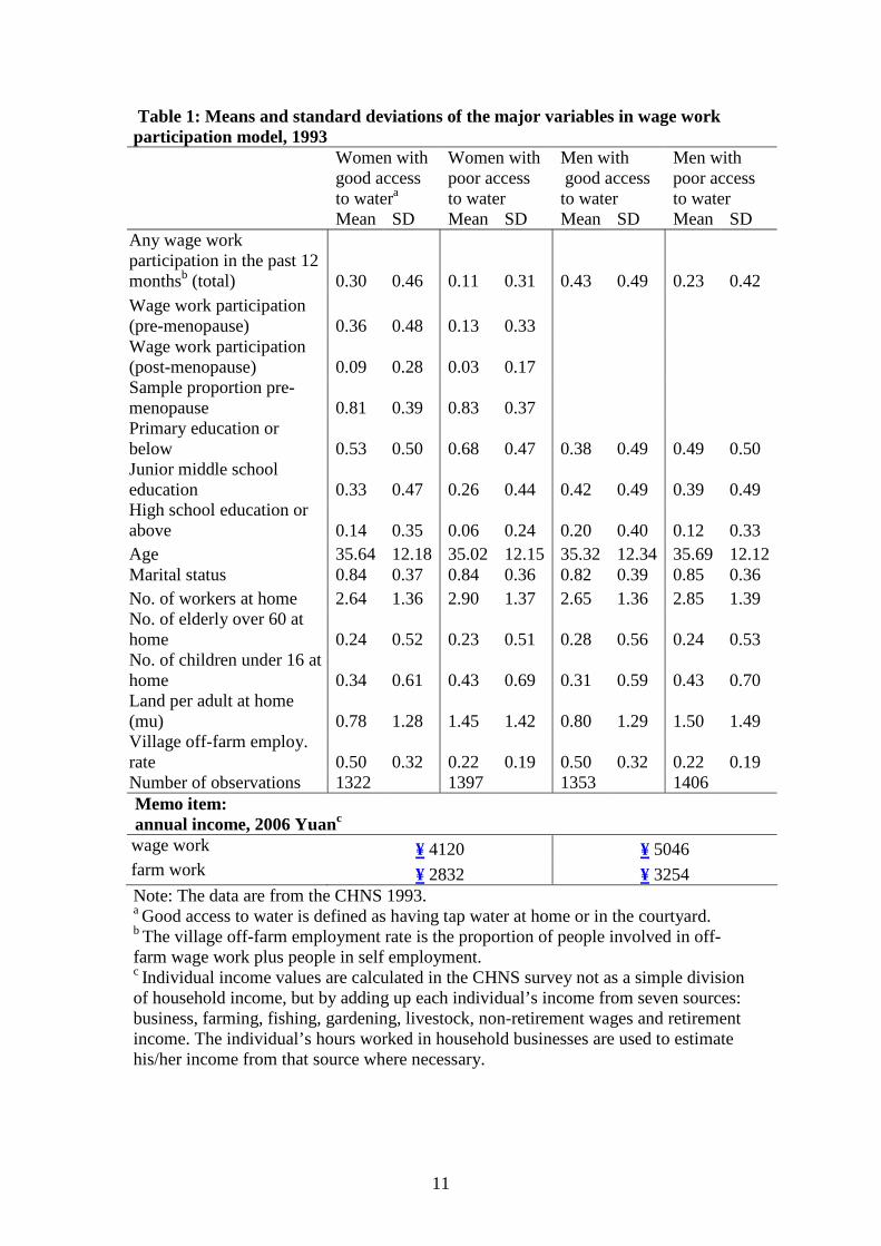
Our work is most closely related that of Hare (1999) and Zhang et al (2002) whoalso investigate determinants of the wage work status in China. Following Hare(1999), we construct a ‘wage work participant’ status dummy variable dependingupon whether the respondent has been involved in wage work activity as an employeeduring the last 12 months. (Note, we include all self-employed in the non-wage workcategory.) The relevant percentages, by household water access, are given in Table 1:As can be seen, men in general participate more in wage work than women, and wagework (see memo items in the bottom rows) pays much better than farm work. Alsogood household access to water is correlated with more wage work, for both sexes,presumably because of the better economic environment in which household withgood water access find themselves. Thus, the village average off-farm employmentrate is 50% in good access to water areas, and only 22% in poor access areas.Moreover, individuals, both male and female, are better educated in the good accessto water categories, indicating a sorting of the more productive workers into the moreproductive areas.

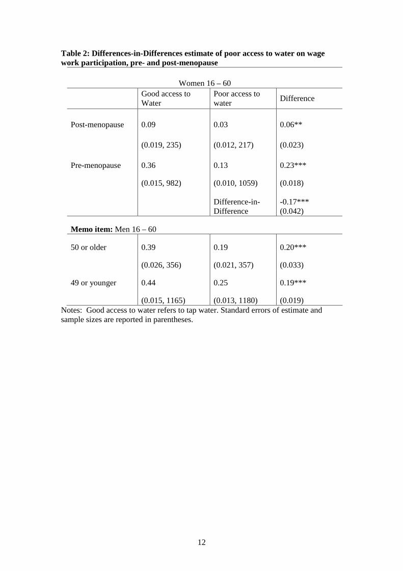
However, following our hypothesis, note the bigger impact of poor access towater for the pre-menopause women, 23 percentage points (=36–13) than for post-menopause women, 6 percentage points (=9–3), or men, 20 points (=43–23). Thisdifference in difference analysis can be pursued using Table 2, pointing to a possiblerole for menopause in explaining the impact of poor access to water, though of courselocal economic development which is correlated with poor access to water must becontrolled.

5

The control variables included in the regression, apart from access to water andmenopause, are similar to those used in (Hare, 1999 and Zhang et al., 2002). Therespondent’s educational qualifications and age are included as measures of humancapital which act as proxy for the expected wage offer. Family structure variables arealso included to allow for supply side effects on wage work participation. Under thisheading come marital status, the number of elderly people over 60 who are present inthe home, and numbers of children present in the home. Some of these variables canbe expected to affect women pre- and post-menopause, and men, differently, and socross-products will be required. Also included in the regression is land owned perfamily adult member, which will affect alternatives to wage work.

Judging by the statistics shown in Table 1, poor access to water is likely to beassociated with backward geographical location and a generally unfavourable villageenvironment. These factors may generate a “culture” unfavourable to women (forexample see Song et al 2006). To tackle this problem, we control for the proportion ofoff-farm employment in the village. As a further control, we include 128 villagedummies, converting the analysis to a within-village analysis. “Culture” effects willthus have to be interpreted as applying to only part of a village, which is possible, butless likely.

A further problem is that unobserved individual characteristics (e.g., an activeattitude for hygiene and work) may be positively correlated with wage workparticipation and access to good water. This linkage would cast doubt on theexogeneity of access to tap water, raising the need for instrumentation. In fact, wefind that government investment in village water construction (variable water planthereafter) is a good instrument – well correlated with the probability of a householdhaving access to tap water, but not directly linked to an individual’s wage workparticipation. We therefore have a reasonable basis to test for endogeneity.

4. Empirical Strategies

Regression Analysis. To study the interaction of access to water and menstrual cycle,we use a difference-in-difference specification:

Yi = β1 + β2Wi+ β3Mi+ β4WiMi + β5Xi + φs + εi

where i denotes individuals; Yi is an indicator for having participated in any wagework during the last 12 months; Xi is a vector of controls for individual and householdcharacteristics; Wi is an indicator equal to one if the household has no access to tapwater; Mi is an indicator equal to one if the individual is pre-menopause; φs is a full setof 128 village dummies (for small samples, 36 county dummies); and εi is the errorterm.

β4 is the coefficient of interest. We expect poor access to water to have a moreadverse impact on pre-menopause women’s wage work participation, due to thehygiene/time/psychic related menstrual problems they face as described earlier. Theseconsiderations point to a negative interaction between the access to water andmenstrual cycle. The adverse impact of poor access to water on pre-menopausewomen (β2) is expected to be small or zero. In order to allow full variation of theimpacts of the other control variables, we also estimate probit models for these twogroups of women separately. In this case, for pre-menopause women we have:

Yi = (β1 + β3) + (β2+ β4 )Wi + β5Xi + φs + εi

6

showing that the coefficient on W is the sum of both β2 and β4, while for post-menopause women we have simply:

Yi = β1 + β2Wi + β5Xi + φs + εi

Thus, we can recover β4 simply by comparing the coefficient on W in the tworegressions.

After estimating the probit coefficients, we calculate average marginal effects(AME) of the regressors since estimating the AME is recommended for policyanalysis (Cameron and Trivedi, 2009, 340). (Where there are many cross-products,however, we simply give the raw probit coefficients (see Bartus 2005), since AMEare then misleading.) The AME may also be more comparable to the averagetreatment on the treated (ATT) that is to be obtained in the second phase of thisresearch via Propensity Score matching techniques, since both of these measureaverage effects of a treatment on those who received the treatment.

Propensity Score Matching. Regression analysis provides a complete mechanism toanalyse treatment effects, but only in ideal circumstances, and Propensity ScoreMatching (PSM) (see Caliendo and Kopeinig, 2008; Imbens and Wooldridge, 2009)might be more robust. In the regression case, a full model is estimated which gives acheck on the plausibility of the model as a whole, and on effect sizes for manyvariables of interest. On the other hand, selection bias needs to be tackled byincluding all ‘necessary’ variables in the regression as controls (the so called ‘longmodel’) and appropriate instrumentation (see Angrist and Pischke, 2009), which isobviously difficult to do.

PSM works by making the assignment of the poor access to water “treatment”random between the comparison groups. A ‘score’ based on a logit determining pooraccess to water is estimated for all individuals in the sample. This ‘propensity score’is the conditional probability of receiving the poor access to water treatment givenpre-treatment characteristics (Rosenbaum and Rubin, 1983). The sample is thenseparated into about five different blocks or strata (Imbens and Wooldridge, 2009, 33)according to the propensity scores so that within each block the propensity score isessentially constant and the data can be taken as coming from a randomisedexperiment. The effect of the treatment is then identified within each block and theaverage taken across blocks to give the average treatment effect on the treated (ATT).

PSM reduces the effect of unobserved, possibly endogenous (see Frolich, 2008),factors causing differences between treated and controls by accurate matching (but fora warning see Pearl, 2009). Matching is assisted by the blocking technique notedabove, and also via the “common support” requirement. This requirement involvesdropping individuals in the treatment group who have a probability of poor access towater that lies outside the range for the control group. Admittedly this commonsupport requirement results in dropping many observations (see below), which raisesthe problem of whether effects measured via PSM are representative of the broaderpopulation. However, if our results using regression analysis on the whole sample aresimilar to results for PSM we will be reassured. A further factor important formatching (Heckman et al, 1997) is that both treated and controls reside in the samenarrowly-defined local labour markets, in our case, rural villages.

7

We make the propensity score logit for poor access to water depend upongovernment investment in water construction in the individual’s village (water plant),and all 128 village dummies. We also include a broad set of further variables (seeCaliendo and Kopeinig, 2008) on individual and household level characteristicsrelevant to wage work participation. Then, to match treatment and control groups weuse four common matching techniques: Nearest neighbour, Radius, Kernel andStratification matching. Each has its own advantages and disadvantages (see Beckerand Ichino, 2002), and we report outcomes for all.

5. The Results

Regression results. First, we estimate an IV probit model for women and menseparately to test the exogeneity of the poor access to water variable for wage workparticipation models. Table 3 shows that the impact of poor access to water is onlysignificant for women. It is also quantitatively large, -0.50 for the pre-menopausegroup. In fact, for all groups in Table 3, the Wald test indicates that poor water accessis exogenous, so we will proceed on that basis.

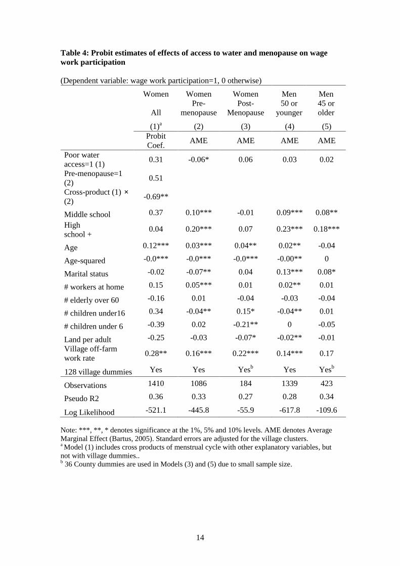
Table 4 then presents probits for various groups. Most models include all 128village fixed effects, though samples for models (3) and (5) are too small, and so only36 county effects incorporated. In the first column, results for a sample pooling allwomen are given which shows explicitly the separate effects of poor access to water,menopause, and their interaction. As can be seen, the cross-product is significant, andit is large, -0.69. The effect of poor water access alone is -0.38 (=-0.69+0.31),somewhat smaller than the IV result shown in Table 3 (-0.46) indicating somedownward bias results from the ordinary probit approach. In columns (2) and (3),results are given for the pre- and post-menopause groups separately, and since cross-products are not needed, average marginal effects (AMEs) can be calculated. Twoprobit models are also estimated for men aged 50 or younger and over 45 forcomparison purposes (the age spans chosen generally match the age spans of pre- andpost-menopause women in the sample).

As can be seen from Table 4, the effect of poor access to water is onlysignificant for women pre-menopause, while it is virtually zero for post-menopausewomen and men after controlling for other factors. The AME of poor access to water(column 2) implies that poor access to water reduces the probability of wage workparticipation for women pre-menopause by 6 percentage points, holding other thingsequal.

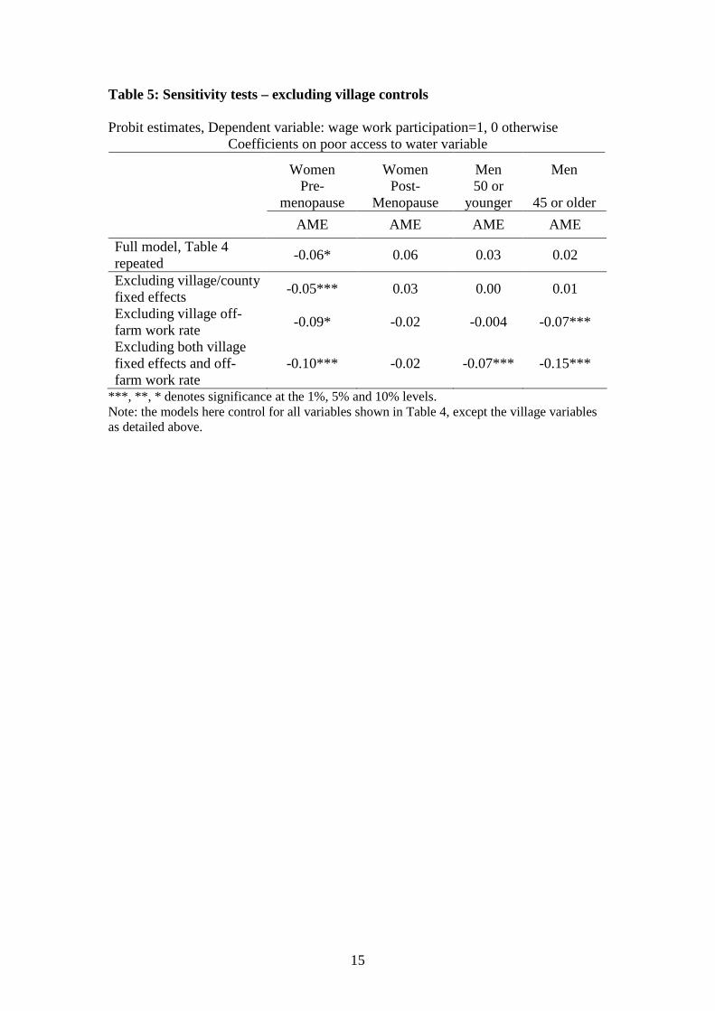
It is interesting that poor water access has so little effect on men’s wage workparticipation, ceteris paribus, despite its strong association with participation in Table2. However, we are controlling for the village off-farm work rate, and also villagefixed effects, all of which pick up local opportunities for wage work, and arecorrelated with poor water access. Table 5 shows that if we exclude village controls(the village fixed effects, and village off-farm work rates) from the probits, the pooraccess to water variable becomes significant for men. We conclude that while localopportunities for wage work play an important role for all groups, this fact does notoverturn our hypothesis that poor water access plays an independent role negativelyimpacting pre-menopause women.

8

Most other variables have the signs expected. Having children under 6 in thehousehold has a particular negative impact (-0.21) on post-menopause women’s wagework participation while it has virtually no impact for other groups. This findingrelates to the low wage work participation for this group (Table 2), and chimes in withthe fact that in rural China, older women often look after young children to supportyounger women and men at work (Entwissle and Chen, 2002)

Finally, it must be emphasised that village dummies are included in the model topick up unobserved village fixed effects – e.g. culture and remote geography. Whilesome village dummies have to be dropped due to collinearities in the regression, manyof the remaining villages possess significant fixed effects, a fact that shows theimportance of controlling at the village level.

PSM results. The covariates included in the logit models to derive the propensityscores are generally the same with those in IV probit models in Table 3 (first stage),apart from the fact that now 128 village dummies are included instead of 36 countydummies. The impacts of covariates however remain generally the same and thereforethe results are not given. The logit model is estimated for men and women (pre-menopause) separately in order to enable covariate balancing before matching. Themost important determinant of poor access to water is government investment invillage water construction (water plant), plus the village fixed effects.

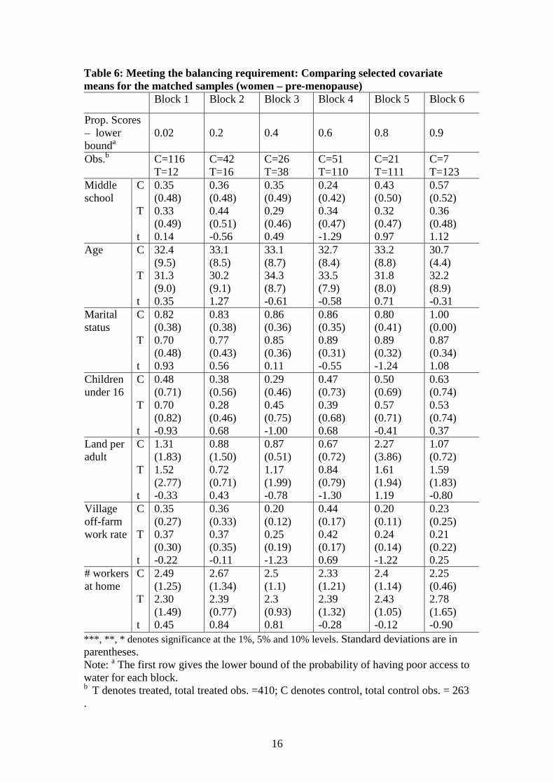
The results of the covariate mean comparisons between treated and controlgroups of women are shown in the Table 6. (Results are not given for men as theyshow the same pattern as for women.). The first row gives the lower bound of theprobability of having poor access to water for each block. For example, in block 2, theprobability of having access to poor water varies from 0.2 to (maximum) 0.39. The t-test results show that the mean values of selected covariates within each block are notdifferent between the treatment and control groups – in fact, there is not a singlesignificant difference (For other covariates not shown in the table, the means are alsofound to be not different.)

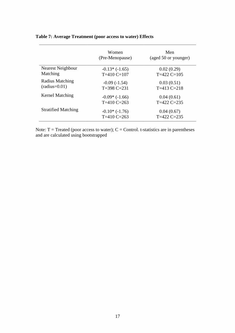
Table 7 gives the estimated ATT results using the four matching techniques. Thetechniques show a similar negative effect of poor access to water on wage workparticipation of women. No impact is found for men. The size of the impact variesbetween –0.09 and –0.13 depending upon technique. Interestingly, this effect isgreater than the –0.06 average marginal effect estimated from the regressions, furtherindicating that some downward bias results from the ordinary probit approach.

An impact of around –0.10 is large, considering the unconditional meandifference of wage work participation between pre-menopause women with good andpoor access to water is about 23 percentage points (Table 1). In other words, about40% (=0.10/0.23) of the disadvantage in wage work participation that women in pooraccess to water households suffer is really due to poor access to water. The remainderis due to factors such as lack of village development which are associated with pooraccess to water. For men, poor access to water has no causal effect on wage workparticipation.

9

6. Conclusions

In this study, we investigate the impact of poor access to water on wage workparticipation in rural China. This study hypothesises that women pre-menopause facehigher costs of participation and achieve lower productivity when access to water ispoor (holding other things equal), and therefore have lower rate of wage workparticipation. We use CHNS data for 1993 to test the hypothesis. In this dataset, abouthalf of the respondents do not have access to improved water, and also a large numberof respondents are not involved in any type of wage work. Most importantly, there isspecific information about women’s menopause status.

We use both regression analysis and PSM methods to test the hypothesis. Bothapproaches yield supportive results. Women pre-menopause are found to beespecially affected by poor access to water, that is, their probability of participating inwage work is about 10 percentage points lower than their peers with good access towater controlling for other confounding factors. For men, poor access to water per sehas no causal impact on wage work participation. Therefore, a major benefit ofpolicies to improve water supplies may not be the obvious household or industrialbenefit, but rather an unseen benefit, the improvement in the working position ofwomen. While much of these benefits have already been gained in China which hasmade good progress in raising access to water, the results should be relevant to otherareas of the developing world.

10

Figure 1: Women’s share in wage work and access to sanitation facilities,developing countries in 2000

Bangladesh

Brazil

Chile

China

Ghana

India

Indonesia

Jamaica

Jordan

Kenya

Malawi

Morocco

Nepal

Nigeria

Peru

Tunisia

Uganda

Tanzania

Zimbabwe

10

20

30

40

50

wom

en

inwage

em

plo

ym

ent(%

)

0 20 40 60 80 100population using improved sanitation facility %

Source: UN (2009)

Figure 2: Trends in household access to water

0

5

10

15

20

25

30

35

40

45

50

1989 1991 1993 1997 2000 2004

In House Tap Water In Yard Tap Water In Yard Well Water Other Water

Source: CHNS 1989 – 2004.

In-house tap water

Other water

In-yard well water

In-yard tap water

11

Table 1: Means and standard deviations of the major variables in wage workparticipation model, 1993

Women withgood accessto watera

Women withpoor accessto water

Men withgood accessto water

Men withpoor accessto water

Mean SD Mean SD Mean SD Mean SDAny wage workparticipation in the past 12monthsb (total) 0.30 0.46 0.11 0.31 0.43 0.49 0.23 0.42

Wage work participation(pre-menopause) 0.36 0.48 0.13 0.33Wage work participation(post-menopause) 0.09 0.28 0.03 0.17Sample proportion pre-menopause 0.81 0.39 0.83 0.37Primary education orbelow 0.53 0.50 0.68 0.47 0.38 0.49 0.49 0.50Junior middle schooleducation 0.33 0.47 0.26 0.44 0.42 0.49 0.39 0.49High school education orabove 0.14 0.35 0.06 0.24 0.20 0.40 0.12 0.33

Age 35.64 12.18 35.02 12.15 35.32 12.34 35.69 12.12Marital status 0.84 0.37 0.84 0.36 0.82 0.39 0.85 0.36

No. of workers at home 2.64 1.36 2.90 1.37 2.65 1.36 2.85 1.39No. of elderly over 60 athome 0.24 0.52 0.23 0.51 0.28 0.56 0.24 0.53No. of children under 16 athome 0.34 0.61 0.43 0.69 0.31 0.59 0.43 0.70Land per adult at home(mu) 0.78 1.28 1.45 1.42 0.80 1.29 1.50 1.49Village off-farm employ.rate 0.50 0.32 0.22 0.19 0.50 0.32 0.22 0.19Number of observations 1322 1397 1353 1406Memo item:annual income, 2006 Yuanc

wage work ¥ 4120 ¥ 5046farm work ¥ 2832 ¥ 3254Note: The data are from the CHNS 1993.a Good access to water is defined as having tap water at home or in the courtyard.b The village off-farm employment rate is the proportion of people involved in off-farm wage work plus people in self employment.c Individual income values are calculated in the CHNS survey not as a simple divisionof household income, but by adding up each individual’s income from seven sources:business, farming, fishing, gardening, livestock, non-retirement wages and retirementincome. The individual’s hours worked in household businesses are used to estimatehis/her income from that source where necessary.

12

Table 2: Differences-in-Differences estimate of poor access to water on wagework participation, pre- and post-menopause

Women 16 – 60

Good access toWater

Poor access towater

Difference

Post-menopause 0.09 0.03 0.06**

(0.019, 235) (0.012, 217) (0.023)

Pre-menopause 0.36 0.13 0.23***

(0.015, 982) (0.010, 1059) (0.018)

Difference-in-Difference

-0.17***(0.042)

Memo item: Men 16 – 60

50 or older 0.39 0.19 0.20***

(0.026, 356) (0.021, 357) (0.033)

49 or younger 0.44 0.25 0.19***

(0.015, 1165) (0.013, 1180) (0.019)Notes: Good access to water refers to tap water. Standard errors of estimate andsample sizes are reported in parentheses.

13

Table 3: The effect of access to water on wage work participation – instrumentalvariables results (IV)

IV Probit All WomenWomen Pre-menopause

All Men

Coef z Coef z Coef zSecond Stage – Dependent Variable: wage work participation=1, 0 otherwisePoor water access -0.46*** -2.86 -0.50*** -2.73 -0.13 -1.00Middle school 0.42*** 4.19 0.45*** 4.09 0.35*** 4.18High school + 0.75*** 5.58 0.78*** 5.36 0.84*** 7.99Age 0.13*** 4.10 0.13*** 2.33 0.10*** 4.02Age-squared -0.00*** -4.98 -0.00** -2.42 -0.00*** -4.41Marital status -0.17 -1.03 -0.35* -1.65 0.19 1.34# workers at home 0.17*** 4.81 0.20*** 4.43 0.07** 2.25# elderly over 60 -0.02 -0.25 0.03 0.36 -0.14 -1.55# children under16 -0.18* -1.61 -0.20 -1.58 -0.15* -1.75# children under 6 0.03 0.23 0.12 0.76 0.02 0.16Land per adult -0.17*** -3.49 -0.16*** -3.17 -0.11*** -3.42Village off-farmwork rate 0.75*** 8.49 0.76*** 7.67 0.59*** 10.24County (36)dummies Yes Yes YesFirst Stage – Dependent Variable: Poor access to water=1, 0 otherwiseWater Plant -0.88*** -3.48 -0.88*** -2.86 -0.91*** -3.29Middle school 0.01 0.35 0.01 0.49 0.02 0.84High school + 0.02 0.77 0.02 0.51 -0.01 -0.40Age -0.01 -1.29 0.00 0.13 0.00 -0.69Age-squared 0.00 1.58 -0.00 -0.10 0.00 0.98Marital status 0.01 0.54 -0.00 -0.01 0.03 1.10# workers at home 0.00 0.73 0.01 0.64 0.00 0.12# elderly over 60 0.05 3.02 0.03* 1.73 0.04* 1.92# childr. under16 -0.01 -0.39 -0.01 -0.29 -0.01 -0.33# childr. under 6 0.01 0.36 0.00 0.09 0.01 0.32Land per adult 0.00 0.35 0.00 0.62 0.00 -0.06Village off-farmwork rate -0.03** -2.34 -0.03** -2.10 -0.02* -1.60County (36)dummies Yes Yes YesWald Test ofExogeneity,prob>Chi2 0.19 0.35 0.69Observations 2033 1469 1864Log likelihood -1274.8 -977.5 -1441.8Note: ***, **, * denotes significance at the 1%, 5% and 10% levels. Standard errors areadjusted for the county clusters. The inclusion of village dummies is not possible for IVprobit due to non-concavity, but they are included in the main probit models in Table 4. Theimpact of poor access to water is insignificant for women post-menopause in a separate IVprobit model (results not shown, but similar results are given in Table 4).

14

Table 4: Probit estimates of effects of access to water and menopause on wagework participation

(Dependent variable: wage work participation=1, 0 otherwise)

Women Women Women Men Men

AllPre-

menopausePost-

Menopause50 or

younger45 orolder

(1)a (2) (3) (4) (5)ProbitCoef.

AME AME AME AME

Poor wateraccess=1 (1)

0.31 -0.06* 0.06 0.03 0.02

Pre-menopause=1(2)

0.51

Cross-product (1) ×(2)

-0.69**

Middle school 0.37 0.10*** -0.01 0.09*** 0.08**

Highschool +

0.04 0.20*** 0.07 0.23*** 0.18***

Age 0.12*** 0.03*** 0.04** 0.02** -0.04

Age-squared -0.0*** -0.0*** -0.0*** -0.00** 0

Marital status -0.02 -0.07** 0.04 0.13*** 0.08*

# workers at home 0.15 0.05*** 0.01 0.02** 0.01

# elderly over 60 -0.16 0.01 -0.04 -0.03 -0.04

# children under16 0.34 -0.04** 0.15* -0.04** 0.01

# children under 6 -0.39 0.02 -0.21** 0 -0.05

Land per adult -0.25 -0.03 -0.07* -0.02** -0.01

Village off-farmwork rate

0.28** 0.16*** 0.22*** 0.14*** 0.17

128 village dummies Yes Yes Yesb Yes Yesb

Observations 1410 1086 184 1339 423

Pseudo R2 0.36 0.33 0.27 0.28 0.34

Log Likelihood -521.1 -445.8 -55.9 -617.8 -109.6

Note: ***, **, * denotes significance at the 1%, 5% and 10% levels. AME denotes AverageMarginal Effect (Bartus, 2005). Standard errors are adjusted for the village clusters.a Model (1) includes cross products of menstrual cycle with other explanatory variables, butnot with village dummies..b 36 County dummies are used in Models (3) and (5) due to small sample size.

15

Table 5: Sensitivity tests – excluding village controls

Probit estimates, Dependent variable: wage work participation=1, 0 otherwiseCoefficients on poor access to water variable

Women Women Men MenPre-

menopausePost-

Menopause50 or

younger 45 or older

AME AME AME AME

Full model, Table 4repeated

-0.06* 0.06 0.03 0.02

Excluding village/countyfixed effects

-0.05*** 0.03 0.00 0.01

Excluding village off-farm work rate

-0.09* -0.02 -0.004 -0.07***

Excluding both villagefixed effects and off-farm work rate

-0.10*** -0.02 -0.07*** -0.15***

***, **, * denotes significance at the 1%, 5% and 10% levels.Note: the models here control for all variables shown in Table 4, except the village variablesas detailed above.

16

Table 6: Meeting the balancing requirement: Comparing selected covariatemeans for the matched samples (women – pre-menopause)

Block 1 Block 2 Block 3 Block 4 Block 5 Block 6

Prop. Scores– lowerbounda

0.02 0.2 0.4 0.6 0.8 0.9

Obs.b C=116T=12

C=42T=16

C=26T=38

C=51T=110

C=21T=111

C=7T=123

C 0.35(0.48)

0.36(0.48)

0.35(0.49)

0.24(0.42)

0.43(0.50)

0.57(0.52)

T 0.33(0.49)

0.44(0.51)

0.29(0.46)

0.34(0.47)

0.32(0.47)

0.36(0.48)

Middleschool

t 0.14 -0.56 0.49 -1.29 0.97 1.12C 32.4

(9.5)33.1(8.5)

33.1(8.7)

32.7(8.4)

33.2(8.8)

30.7(4.4)

T 31.3(9.0)

30.2(9.1)

34.3(8.7)

33.5(7.9)

31.8(8.0)

32.2(8.9)

Age

t 0.35 1.27 -0.61 -0.58 0.71 -0.31C 0.82

(0.38)0.83(0.38)

0.86(0.36)

0.86(0.35)

0.80(0.41)

1.00(0.00)

T 0.70(0.48)

0.77(0.43)

0.85(0.36)

0.89(0.31)

0.89(0.32)

0.87(0.34)

Maritalstatus

t 0.93 0.56 0.11 -0.55 -1.24 1.08C 0.48

(0.71)0.38(0.56)

0.29(0.46)

0.47(0.73)

0.50(0.69)

0.63(0.74)

T 0.70(0.82)

0.28(0.46)

0.45(0.75)

0.39(0.68)

0.57(0.71)

0.53(0.74)

Childrenunder 16

t -0.93 0.68 -1.00 0.68 -0.41 0.37C 1.31

(1.83)0.88(1.50)

0.87(0.51)

0.67(0.72)

2.27(3.86)

1.07(0.72)

T 1.52(2.77)

0.72(0.71)

1.17(1.99)

0.84(0.79)

1.61(1.94)

1.59(1.83)

Land peradult

t -0.33 0.43 -0.78 -1.30 1.19 -0.80C 0.35

(0.27)0.36(0.33)

0.20(0.12)

0.44(0.17)

0.20(0.11)

0.23(0.25)

T 0.37(0.30)

0.37(0.35)

0.25(0.19)

0.42(0.17)

0.24(0.14)

0.21(0.22)

Villageoff-farmwork rate

t -0.22 -0.11 -1.23 0.69 -1.22 0.25C 2.49

(1.25)2.67(1.34)

2.5(1.1)

2.33(1.21)

2.4(1.14)

2.25(0.46)

T 2.30(1.49)

2.39(0.77)

2.3(0.93)

2.39(1.32)

2.43(1.05)

2.78(1.65)

# workersat home

t 0.45 0.84 0.81 -0.28 -0.12 -0.90

***, **, * denotes significance at the 1%, 5% and 10% levels. Standard deviations are inparentheses.Note: a The first row gives the lower bound of the probability of having poor access towater for each block.b T denotes treated, total treated obs. =410; C denotes control, total control obs. = 263.

17

Table 7: Average Treatment (poor access to water) Effects

Women(Pre-Menopause)

Men(aged 50 or younger)

Nearest NeighbourMatching

-0.13* (-1.65)T=410 C=107

0.02 (0.29)T=422 C=105

Radius Matching(radius=0.01)

-0.09 (-1.54)T=398 C=231

0.03 (0.51)T=413 C=218

Kernel Matching -0.09* (-1.66)T=410 C=263

0.04 (0.61)T=422 C=235

Stratified Matching -0.10* (-1.76)T=410 C=263

0.04 (0.67)T=422 C=235

Note: T = Treated (poor access to water); C = Control. t-statistics are in parenthesesand are calculated using bootstrapped

18

REFERENCES:

Ahmed, R., and Yesmin, K. (2008) “Menstrual Hygiene: Breaking the Silence”, inWateraid, Beyond Construction – A collection of case studies from sanitationand hygiene promotion practitioners in South Asia, London: Water Aid, 2009.

Angrist, J., D. and Pischke, J-S (2009) Mostly Harmless Econometrics, PrincetonUniversity Press, Princeton and Oxford

Bharadwaj, S., and Archana, P. (2004) “Menstrual Hygien and Management inDeveloping Countries: Taking Stock”, Mumbai: Junction Social.

Bartus, T. (2005) “Estimation of Marginal Effects Using margeff”, The Stata Journal,5 (3): pp. 309-329

Becker, S., and A. Ichino (2002) “Estimation of Average Treatment Effects Based onPropensity Scores,” The Stata Journal 2 (4): pp. 358–377

Benjamin, D., Brandt, l., Glewwe, P., and Li, G. (2000) “Markets, Human Capital andInequality: Evidence from Rural China”, University of Michigan BusinessSchool Working Paper No.298.

Bryson A., Dorsett, R. and Purdon, S. (2002). “The Use of Propensity Score Matchingin the Evaluation of Active Labour Market Policies”, Working Paper Number 4,London: Department of Work and Pensions.

Burns N., Scholzman K., and Verba S. (1997). “The Public Consequences of PrivateInequality: Family Life and Citizen Participation”, The American PoliticalScience Review, 91 (2): 373-89.

Burrows, G., Acton, J., and Maunder, T. (2004) Water and Sanitation: the EducationDrain, London: Wateraid,http://www.wateraid.org/other/startdownload.asp?DocumentID=113

Caliendo, M.and Kopeinig, S. (2008) “Some Practical Guidance for theImplementation of Propensity Score Matching”, Journal of Economic Surveys,22: 31-72.

Cameron, A., C. and Trivedi, P., K. (2005) Microeconometrics: Methods andApplications, Cambridge, New York

Cameron, A., C. and Trivedi, P., K. (2009) Microeconometrics Using Stata, StataPress, Texas

Chawla, A., Swindle, R., Long, S., Kennedy S., and Steinfeld, B. (2002).“Premenstrual Dysphoric Disorder – Is There an Economic Burden of Illness?”,Medical Care 40 (11): 1101-12.

Chhibber, P. (2002). “Why Are Some Women Politically Active? The Household,Public Space and Political Participation in India”, International Journal ofComparative Sociology, 43: 409-29.

CHNS (2009) China Health and Nutrition Survey, Chapel Hill, North Carolina:Carolina Population Center, http://www.cpc.unc.edu/projects/china

Dean, B., and Borenstein, J. (2004). “A Prospective Assessment Investigating theRelationship between Work Productivity and Impairment with PremenstrualSyndrome”, Journal of Occupational and Environmental Medicine, 46 (7): 649-56.

Deuster P., Adera T., and South-Paul J. (1999). “Biological, Social and BehaviouralFactors Associated with Premenstrual Syndrome”, Archives of FamilyMedicine, 8: 122-28.

19

Entwisle, B., and Chen, F-N (2002) “Work Patterns Following a Birth in Urban andRural China: A Longitudinal Study”, European Journal of Population, 18:pp.99-119

Field, E. and Arbus, A. (2008) “Early Marriage, Age of Menarche and FemaleSchooling Attainment in Bangladesh”, Journal of Political Economy, 116(5):881-930.

Flabbi, L., and Ichino, A. (2001) “Productivity, Seniority and Wages: New Evidencefrom Personnel Data”, Labour Economics, 8: pp 359-387.

Frolich, M. (2008). “Parametric and Nonparametric Regression in the Presence ofEndogenous Control Variables”, International Statistical Review, 76: 214-227.

Galiani S., Gonzalez-Rozada M., and Schargrodsky E. (2009) “Water Expansions inShantytowns: Health and Savings”, Economica 76: 607-22.

Galiani S., Gertler P., and Schargrodsky E. (2005). “Water for Life: The Impact of thePrivatization of Water Services on Child Mortality”, Journal of PoliticalEconomy, 113: 83-120.

Glaeser, E., Ponzetto G., and Shleifer, A. (2007) “Why Does Democracy NeedEducation?”, Journal of Economic Growth, 12: 77-99.

Goldin C., and Katz L. (2002). “The Power of the Pill: Oral Contraceptives andWomen’s Career and Marriage Decisions”, Journal of Political Economy, 110(4): 730-70.

Guo, S-Y, and Fraser, M., W. (2009) Propensity Score Matching, Sage, LondonHare, D. (1999) “Women’s Economic Status in Rural China: Household

Contributions to Male-Female Disparities in the Wage-Labour Market”, WorldDevelopment, 27(6): pp 1011-1029

Heckman, J., Ichimura, H., and Todd, P. (1997) “Matching as a EconometricEvaluation Estimator: Evidence from Evaluating a Job Training Programme”,Review of Economic Studies, 64: 605-54.

Ichino, A. and Moretti, E. (2009) “Biological Gender Differences, Absenteeism andthe Earning Gap”, American Economic Journal: Applied Economics, 1(1): pp.183-218

Imbens, G. and Wooldridge, J. (2009) “Recent Developments in the Econometrics ofProgram Evaluation”, Journal of Economic Literature, 47: 5-86.

Iversen T., and Rosenbluth, R. (2006). “The Political Economy of Gender: ExplainingCross-National Variation in the Gender Division of Labor and the GenderVoting Gap”, American Journal of Political Science, 50 (1): 1-19.

Jacka, T. (1997) Women's Work in Rural China: Change and Continuity in an Era ofReform, Cambridge University Press, Cambridge

Jalan, J., and Ravallion, M (2003) “Does piped water reduce diarrhoea for children inrural India?”, Journal of Econometrics, 112: pp153-173

Kirk, J. and Sommer, M. (2006) “Menstruation and Body Awareness: Critical Issuesfor Girls’ Education”, EQUALS, 15: pp 4-5.

Maimaiti, Y. and Siebert, W. S. (2009) “The Gender Education Gap in China – ThePower of Water”, IZA Discussion Paper 4018

Mangyo E. (2008). “The Effect of Water Accessibility on Child Health in China”,Journal of Health Economics 27: 1343-56.

Oster, E., and Thornton, R (2009) “Menstruation and Education in Nepal”, NBERworking paper, 14853.

Pearl, J. (2009). Causality, 2d edition, Cambridge: Cambridge University PressRosenbaum, P., and Rubin, D (1983) “The Central Role of the Propensity Score in

Observational Studies for Causal Effects,” Biometrika, 70, pp.41–55

20

Sicular, T., and Zhao, Y-H (2004) “Earnings and Labour Mobility in Rural China:Implications for China’s Accession to the WTO”, In China and the WTO:Accession, Policy Reform and Poverty Reduction Strategies (Ed: Bhattasali, D.,Li, S-T, Martin, W), The World Bank, Oxford University Press, pp. 239-260

Song, L., and Appleton, S., and Knight, J., 2006, “Why Do Girls in Rural China HaveLower School Enrolment?” World Development, 34(9), 1639_1653

UN (2009) Millennium Development Goals Indicators Database,http://mdgs.un.org/unsd/mdg/Data.aspx

UNICEF (2009). Unicef and Education: Menstruating Girls, Aspen Design Summit,November 11-14, Aspen Colorado

Wateraid (2009). Beyond Construction – A collection of case studies from sanitationand hygiene promotion practitioners in South Asia, London: Water Aid

Wang G. (2007). “Testing the Impact of Gender Equality on Reproductive Health: AnAnalysis of Developing Countries”, The Social Science Journal 44: 507-24.

Stewart F., Shields, W., and Hwang A. (2004). “Cairo Goals for Reproductive Health:Where Do We Stand at 10 Years?” Contraception 70: 1-2.

Yang, J. H. (2006) “Has the One-Child Policy Improved Adolescents’ EducationalWellbeing in China?” __ CHNS discussion paper 2006.

Zhang, L-X, de Brauw, A., and Rozelle, S (2004) “China’s Rural Labour MarketDevelopment and Its Gender Implications”, China Economic Review, 15: pp.230-247

Zhang, L-X, Huang J-K, and Rozelle, S. (2002) “Employment, Emerging LabourMarkets and the Role of Education in Rural China”, China Economic Review,13: pp. 313-328