Full Terms & Conditions of access and use can be found athttp://www.tandfonline.com/action/journalInformation?journalCode=unht20

Download by: [East China University of Science and Technology], [Dr Zuojin Zhu] Date: 21 December 2016, At: 17:15

Numerical Heat Transfer, Part A: ApplicationsAn International Journal of Computation and Methodology

ISSN: 1040-7782 (Print) 1521-0634 (Online) Journal homepage: http://www.tandfonline.com/loi/unht20

LES of convective heat transfer andincompressible fluid flow past a square cylinder

Xiaowang Sun, C. K. Chan, Bowen Mei & Zuojin Zhu

To cite this article: Xiaowang Sun, C. K. Chan, Bowen Mei & Zuojin Zhu (2016) LES of convectiveheat transfer and incompressible fluid flow past a square cylinder, Numerical Heat Transfer,Part A: Applications, 69:10, 1106-1124

To link to this article: http://dx.doi.org/10.1080/10407782.2015.1109386

Published online: 23 Mar 2016.

Submit your article to this journal

Article views: 98

View related articles

View Crossmark data

Citing articles: 2 View citing articles

NUMERICAL HEAT TRANSFER, PART A 2016, VOL. 69, NO. 10, 1106–1124 http://dx.doi.org/10.1080/10407782.2015.1109386

LES of convective heat transfer and incompressible fluid flow past a square cylinder Xiaowang Suna, C. K. Chanb, Bowen Meia, and Zuojin Zhua,b

aFaculty of Engineering Science, University of Science and Technology of China, Hefei, P.R. China; bDepartment of Applied Mathematics, The Hong Kong Polytechnic University, Kowloon, Hong Kong

ABSTRACT This paper presents large eddy simulation (LES) results of convective heat transfer and incompressible-fluid flow around a square cylinder (SC) at Reynolds numbers in the range from 103 to 3.5 � 105. The LES uses the swirling-strength based sub-grid scale (SbSGS) model. Several flow proper-ties at turbulent regime are explored, including lift and drag coefficients, time-spanwise averaged sub-grid viscosity, and Kolmogorov micro-scale. Local and mean Nusselt numbers of convective heat transfer from the SC under isothermal wall temperature are predicted and compared with empirical results.

ARTICLE HISTORY Received 23 June 2015 Accepted 28 August 2015

1. Introduction

Incompressible turbulent flows past a square cylinder (SC) are important in engineering science, and numerical solutions are useful for the understanding of the flow characteristics. A literature review for the work before 1990 was given previously by Zhu [1], and some academic backgrounds are addressed in this paper.

The heat transfer from SC was measured by Hilpert [2] and Igarishi [3], as reported in [4, 5]. The experimental work of Igarashi was done in a low speed wind tunnel with rectangular cylinders of height 30 mm heated under constant heat flux. After the wake flow measurements [6–11], Lyn and Rodi [12] conducted some experiments on the flapping shear layer formed by flow separation from the forward corner of a SC, with the associated recirculation region on the sidewall, and they found that the recirculation is an important aspect of some flow properties. For drag forces acting on flat- sided columns, the study encompassed by Tong et al. [13] revealed all chamfering can reduce the drag compared with the sharp-cornered case.

Together with the experimental studies reported recently [14–18], there are also numerical simu-lations [19–34], some based on the k–ε turbulence model [19–21] or direct numerical simulation (DNS) [22–32], with others by means of large eddy simulation (LES) [33, 34]. For turbulent flow simulations, three strategies, phenomenological modeling [35, 36], DNS [37], and LES [38], are usually employed. In recent years, as reported widely [38–46], LES has become a viable and popular simulation tool.

For LES, in addition to the earlier sub-grid scale (SGS) model of Smagorinsky [38], many SGS models have been developed, including the dynamic SGS model given by Germano et al. [47], a sub-sequent modification given by Lilly [48], the SGS model based on the Kolmogorov equation for resolved turbulence given by Cui et al. [49, 50], the model based on algebraic theory [51], the model assuming sub-grid stress to be proportional to the temporal increment of filtered strain rate by

CONTACT Zuojin Zhu Zuojin@ustc.edu.cn Faculty of Engineering Science, University of Science and Technology of China, Jin Zhai Road 96, Hefei 230026, P.R. China. Color versions of one or more of the figures in the article can be found online at www.tandfonline.com/unht. © 2016 Taylor & Francis

Zhu et al. [52], the singular valued SGS model [53], and the recent SGS model based on dynamic estimation of Lagrangian time scale given by Verma and Mahesh [54].

In LES the unclosed stresses are usually modeled by SGS-viscosity models. Alternatively, the nonlinear convective terms may be modified directly \citepHolm, based on these regulations [56–59]. The concept of spectral-vanishing-viscosity can be used to mimic SGS model for LES [60–64].

Turbulent flow is intermittent such that at a local point the flow may be swirling or non-swirling. The commonly used SGS models [38] have assigned artificially dependent sub-grid viscosity without taking care of the intermittency. A novel SGS model has been developed more recently [65, 66], which properly models turbulent flow intermittency.

This paper presents LES results for zero-incident incompressible turbulent flows around a single SC with convective heat transfer under constant wall temperature condition at Reynolds numbers in

Table 2. Re dependence of CL, CD, (νsr)pm, the relevant RMS values, and the Strouhal number.

Rea3 CL CD (νsr)pm CL

0

CD0

ðnsrÞ0p St

1 � 0.0027 1.543 0.5567 0.1440 0.0346 0.1021 0.1079 2 � 0.00542 1.560 1.726 0.120 0.0643 0.3311 0.1079 2.5 � 0.00913 1.594 2.338 0.1302 0.0734 0.5841 0.1079 5. � 0.0250 1.736 5.197 0.1711 0.0781 1.194 0.1079 7.5 � 0.0330 1.770 8.133 0.1776 0.0854 1.705 0.1079 10 � 0.0365 1.788 10.971 0.1817 0.0877 2.723 0.1079 12.5 � 0.0345 1.786 13.959 0.1726 0.0892 3.365 0.1079 25 � 0.0359 1.813 28.953 0.1748 0.0979 6.562 0.1079 50 � 0.0359 1.804 58.421 0.1612 0.0986 14.15 0.1079 75 � 0.0369 1.834 82.453 0.1779 0.1048 16.66 0.1079 100 � 0.0374 1.816 109.57 0.1624 0.1019 24.85 0.1079 125 � 0.0370 1.825 146.23 0.1679 0.1013 34.14 0.1079 150 � 0.0365 1.834 172.91 0.1721 0.1016 39.98 0.1079 200 � 0.0373 1.832 228.38 0.1708 0.1024 43.92 0.1079 250 � 0.0370 1.833 290.74 0.1710 0.1022 71.81 0.1079 275 � 0.0369 1.845 292.59 0.1789 0.1040 60.42 0.1079 300 � 0.0369 1.841 342.65 0.1817 0.1081 65.17 0.1079 325 � 0.0367 1.843 366.75 0.1795 0.1046 81.55 0.1079 350 � 0.0374 1.834 404.23 0.1725 0.1042 89.92 0.1079

aNote that Re3 ¼ Re/103.

Nomenclature

A matrix expression of velocity gradient ∇u aij element of matrix A B spanwise length of square cylinder (m) Cμ artificially defined constant in Eq. (1) d cross-sectional side length of SC (m) fI FSI, factor of swirling-strength

intermittency, given by Eq. (2) k ¼ 1

2 u02i turbulence kinetic energy Num mean Nusselt number p normalized pressure Re ¼ duin/ν Reynolds number Smax assumed allowable total error T temperature (K) Tw temperature on SC wall surface (K) T∞ temperature of incoming flow fluid

u velocity vector uin incoming flow speed (m/s) u, v, w normalized velocity components (m/s) x, y, z Cartesian coordinates ε dissipation rate of k λci swirling-strength (1/s) λ ¼ λcr þ iλci eigenvalue of ∇u ρ fluid density (kg/m3) ν fluid kinematic viscosity (m2/s) νs sub-grid viscosity (m2/s) νsr =νs/ν viscosity ratio (νsr)pm time-averaged (νsr)peak

ðnsrÞ0p root mean square of (νsr)peak

(νsr)peak peak value of νsr

Θ normalized temperature θ normalized temperature fluctuation

Table 1. Computational parameters.

xu/d xd/d yb/d yt/d N1 N2 N3 RaS

8.5 15 8.5 8.5 191 145 41 0.819 aSmax ≈ 0.5%, with actual number if time steps n=13800 relevant to the final time t=170.

NUMERICAL HEAT TRANSFER, PART A 1107

the range of Re ∈ [103, 3.5 � 105]. Nineteen scenarios are presented, as shown in in Table 2, where the SbSGS model is described [65, 66], with the turbulent heat flux expressed under the gradient diffusion assumption [52, 67]. The objective of this paper is to explore numerically the characteristics of the heat and fluid flows past a SC, with particular reference to the three aspects of Reynolds number dependence, distributions of t–z averaged sub-grid viscosity ratio and Kolmogorov micro-scale, and the local and mean Nusselt numbers.

2. Governing equations

2.1. SbSGS model

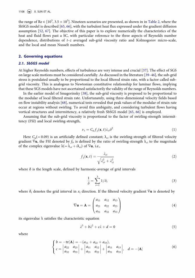
At higher Reynolds numbers, effects of turbulence are very intense and crucial [37]. The effect of SGS on large scale motions must be considered carefully. As discussed in the literature [39–46], the sub-grid stress is postulated usually to be proportional to the local filtered strain rate, with a factor called sub- grid viscosity. This is analogous to Newtonian constitutive relationship for laminar flows, implying that these SGS models have not ascertained satisfactorily the validity of the range of Reynolds numbers.

In the earlier model of Smagorinsky [38], the sub-grid viscosity is proposed to be proportional to the modular of local filtered strain rate. Unfortunately, using three-dimensional velocity fields based on flow instability analysis [68], numerical tests revealed that peak values of the modular of strain rate occur at regions without swirling. To avoid this ambiguity, and considering turbulent flows having vortical structures and intermittency, a relatively fresh SbSGS model [65, 66] is employed.

Assuming that the sub-grid viscosity is proportional to the factor of swirling-strength intermit-tency (FSI) and local swirling-strength,

ns ¼ Cm f Iðx; tÞkcid2 ð1Þ

Here Cμ(¼ 0.09) is an artificially defined constant; λci is the swirling-strength of filtered velocity gradient ∇u, the FSI denoted by fI, is defined by the ratio of swirling-strength λci to the magnitude of the complex eigenvalue λ(¼ λcr þ iλci) of ∇u, i.e.,

f Iðx; tÞ ¼kciffiffiffiffiffiffiffiffiffiffiffiffiffiffiffiffi

k2cr þ k2

ci

q ð2Þ

where δ is the length scale, defined by harmonic-average of grid intervals

1d¼X3

i¼11=di ð3Þ

where δi denotes the grid interval in xi direction. If the filtered velocity gradient ∇u is denoted by

ru ¼ A ¼a11 a12 a13

a21 a22 a23

a31 a32 a33

0

B@

1

CA ð4Þ

its eigenvalue λ satisfies the characteristic equation

k3 þ bk2 þ ckþ d ¼ 0 ð5Þ

where

b ¼ � trðAÞ ¼ � ða11 þ a22 þ a33Þ;

c ¼ a22 a23a32 a33

����

����þ

a11 a12a21 a22

����

����þ

a11 a13a31 a33

����

����; d ¼ � jAj

8<

:ð6Þ

1108 X. SUN ET AL.

with |A| being the determinant of matrix A. For incompressible flows, b ¼ 0. For non-rotating coordinates, the roots of Eq. (5) are real when the local flow is temporally laminar. When the local flow becomes turbulent spontaneously, the roots have two conjugate complex eigenvalues denoted by λcr � iλci, where ið¼

ffiffiffiffiffiffi� 1p

Þ is the unit of imaginary number. Iso-surfaces of swirling-strength have been used to illustrate vortices in turbulent flows previously [69–71].

Assigning the parameter Cμ to be the same value as that used to define turbulent eddy viscosity of phenomenological models [35], the relevant value in the sub-grid model of Vreman [51] has been set as 2:5C2

S. While CS ¼ 0.17 is the theoretical value for homogeneous isotropic turbulence [72], suggest-ing a parametric value of 0.07. Furthermore, to accomplish robust simulations in complex cases the practical value of CS is usually higher. For example, CS ¼ 0.2 has frequently been used in literature, giving a value 0.1. It is noted that in the SGS model of Germano et al. [47], the relevant coefficient is obtained by grid and test-grid filtering, and the coefficient is temporally and spatially changing, hence such kind of model is called a dynamic model.

As the sub-grid viscosity νs has a factor fI, the decaying factor of length scale [1 � exp (� yþ/25)] near the wall as used by Moin and Kim [39] is not used in the present study.

It is noted that swirling-strength does not vanish completely in laminar flows under a rotating framework. To observe the difference in different SGS models, a comparison of the present SbSGS model with that of Vreman [51] is given in Figures 1a, b, where two top-views of the contours of sub-grid viscosity are illustrated. It can be seen that the sub-grid viscosity based on the present model is zero if the local flow is non-swirling, while sub-grid viscosity based on the Vreman’s SGS model does not hold.

2.2. Governing equations

Consider the turbulent SC flow in a Cartesian coordinate system, as schematically shown in Figure 2, in which x(x1) is the horizontal coordinate, with y(x2) and z(x3) denoting the vertical and spanwise directions. The origin is allocated at the left-bottom corner of the SC. Let the incoming flow velocity be uin, the Reynolds number of the SC flow can be defined by Re ¼uind/ν.

Taking the length scale as the SC cross-sectional side length d, the time and pressure scales are t0 ¼ d/uin and qu2

in, where ρ is the fluid density. Therefore, for the zero-incident incompressible heat and fluid flow past a SC, the dimensionless governing equations have the following form:

r � u ¼ 0 ð7Þ

Figure 1. The comparison of the sub-grid model with the previous one proposed by Vreman [51]. (a) A top-view of the contours of νs based on the present model; (b) a top-view of the contours of νs based on the Vreman’s model. Note that the sub-grid viscosity has a unit of W0d0 as seen in Appendix A. The contours in part (a) are labeled by values from 0.0004 to 0.0016 with an increment of 0.0003, while the contours in part (b) are labeled by values from 0.0004 to 0.012 with an increment of 0.0029.

NUMERICAL HEAT TRANSFER, PART A 1109

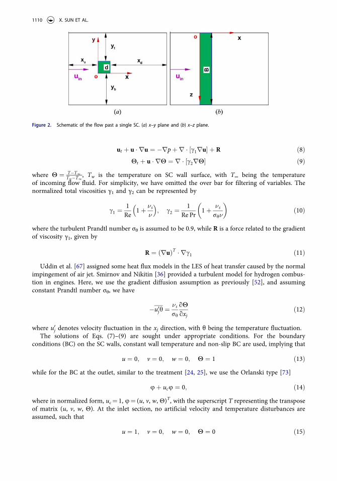
ut þ u � ru ¼ � rpþr � ½c1ru� þ R ð8Þ

Ht þ u � rH ¼ r � ½c2rH� ð9Þ

where H ¼ T� T1Tw� T1, Tw is the temperature on SC wall surface, with T∞ being the temperature

of incoming flow fluid. For simplicity, we have omitted the over bar for filtering of variables. The normalized total viscosities γ1 and γ2 can be represented by

c1 ¼1

Re1þ

ns

n

� �; c2 ¼

1Re Pr

1þns

rhn

� �

ð10Þ

where the turbulent Prandtl number σθ is assumed to be 0.9, while R is a force related to the gradient of viscosity γ1, given by

R ¼ ðruÞT � rc1 ð11Þ

Uddin et al. [67] assigned some heat flux models in the LES of heat transfer caused by the normal impingement of air jet. Smirnov and Nikitin [36] provided a turbulent model for hydrogen combus-tion in engines. Here, we use the gradient diffusion assumption as previously [52], and assuming constant Prandtl number σθ, we have

� u0jh ¼ns

rh

qH

qxjð12Þ

where u0j denotes velocity fluctuation in the xj direction, with θ being the temperature fluctuation. The solutions of Eqs. (7)–(9) are sought under appropriate conditions. For the boundary

conditions (BC) on the SC walls, constant wall temperature and non-slip BC are used, implying that

u ¼ 0; v ¼ 0; w ¼ 0; H ¼ 1 ð13Þ

while for the BC at the outlet, similar to the treatment [24, 25], we use the Orlanski type [73]

uþ ucu ¼ 0; ð14Þ

where in normalized form, uc ¼ 1, u ¼ (u, v, w, Θ)T, with the superscript T representing the transpose of matrix (u, v, w, Θ). At the inlet section, no artificial velocity and temperature disturbances are assumed, such that

u ¼ 1; v ¼ 0; w ¼ 0; H ¼ 0 ð15Þ

Figure 2. Schematic of the flow past a single SC. (a) x–y plane and (b) x–z plane.

1110 X. SUN ET AL.

On the lower and upper side boundaries of the computational domain, we use

uy ¼ 0; v ¼ 0; w ¼ 0; Hy ¼ 0 ð16Þ

On the spanwise boundaries, periodic condition is used such that

uðx; y; z; tÞ ¼ uðx; y; z þ B; tÞ ð17Þ

where B is the spanwise (z) length of SC as shown in Figure 2. The initial condition is given by

u ¼ 1; v ¼ 0; w ¼ 0; H ¼ 0 ð18Þ

3. Numerical method

3.1. Solution procedure

The governing Eqs. (7)–(9) of the heat and fluid flows past a single SC are discretized by a finite difference method in a staggered grid system, where the convective terms are treated using a fourth-order upwind scheme [74]. By making some changes, the existing numerical methods, such as described [75–86] are also applicable. The simple approach recently reported by Trias et al. [87], which on any structured or unstructured grid can be implemented easily, is also suitable for LES of incompressible flows.

The solutions procedure is based on the accurate projection algorithm PmIII developed by Brown et al. [88]. Let intermediate velocity vector, pressure potential, and time level be u, ϕ, and n, respectively. Denoting H ¼ (u·∇)u � R, then letting

unþ1 ¼ u � Dtr/ ð19Þ

we can calculate u by means of

u � un

DtþHnþ1=2 ¼ r � c1r un þ

12ðu � unÞ

� �� �

ð20Þ

and calculate pressure p by

pnþ1=2 ¼ f1 � 0:5ðDtÞr � c1r½ �g/ ð21Þ

where the pressure potential ϕ satisfies the Poisson’s equation

r2/ ¼ r � u=Dt ð22Þ

The temperature Θnþ1 can be calculated by

Hnþ1 � Hn

Dtþ Hnþ1=2

4 ¼ r � c2r Hn þ12ðHnþ1 � HnÞ

� �� �

ð23Þ

where H4 ¼ (u·∇)Θ, and the terms at the level of (n þ 1/2) are calculated explicitly using the second- order Adams–Bashforth formula [89]. Nonlinear convective terms in the governing equations are spatially discretized by a fourth-order upwind finite difference scheme [74], with viscous diffusion terms by a second-order central difference scheme.

The pressure potential Poisson’s equation is initially solved by the approximate factorization one (AF1) method [90], and subsequently corrected by the stabilized bi-conjugate gradient method (Bi- CGSTAB) given by Van der Vorst [91] to improve its accuracy. In the AF1 application, for SC wake flow simulation, the numerical experience reported elsewhere [1] is useful for numerical stability of pressure potential iteration. The criterion for pressure potential iteration is chosen so that the relative

NUMERICAL HEAT TRANSFER, PART A 1111

error defined [89] is less than 1 � 10� 7. In spatial discretization, the implicit second-order Crank– Nicolson method is used to solve the diffusion terms on right-hand side in a non-standard way, where the part depending on the viscosity gradient (∇γ1) in Eq. (10) is calculated explicitly, while the remaining part denoted by [∇·(γ1∇u)] is calculated implicitly.

3.2. Reliability evaluation

In the recent numerical study of Smirnov et al. [92], simulating hydrogen fuel rocket engines using LOGOS simulator [93], an approach for predicting accumulated error in numerical work based on Navier–Stokes equations was reported in detail. As the diffusive terms are treated with the second- order central difference scheme, using the values of N1, N2, and N3 as given in Table 1, and the assumed allowable total error Smax ¼ 0.5%, the ratios of maximum allowable number of time steps to the actual number of time steps used to obtain the result, Rs ¼ 0.819, are estimated and shown in Table 1. This ratio estimation has indicated reliability of the LES results, as reported by Smirnov et al. [92]. The ratio Rs characterizes reliability of results, i.e., how far below the limit the simulations were finalized. Indirectly it characterizes the accumulated error. The higher the value Rs is, the lower is the error. As Rs approaches to unity the error tends to the maximum allowable value.

4. Results and discussion

Using the solution method given above, LES of heat and fluid flows past a single SC, as shown schematically in Figure 2, was encompassed in a personal computer with a memory of 3.2 Gb and CPU frequency 3.30 GHz. Each case requires a CPU time of about 86 hours. As can be seen in Table 2, classified by Re3 ¼ Re/103, 19 scenarios were studied in the LES work. For each scenario the spanwise length of the SC (B) is set at 4.

In the z-direction, the grid is uniform with number Nk set as 41. While the grids are non-uniform in the x- and y-directions, the grid-numbers are set at 191 and 145, respectively, with grid arrange-ments based on a geometric-series algorithm [65]. In this LES, the assignment of grids on the SC section walls uses two key parameters of amplifying-factor (1/0.847) and series termination number (14). The total number of vertical grid-line through the SC cross-sectional side is 34.

At the bottom and top of the SC, the y-grid is assigned with an amplifying-factor of 1/0.9 and a series-termination number of 37. For the x-grid, the relevant values are 1/0.817 and 17, respectively, for the region upstream of the SC, but 1/0.927 and 47 for the region downstream of the SC. Using a geometric-series algorithm for grid partition, it can be seen that the finest grid distance to each SC wall is 2.733 � 10� 3d. Such a grid arrangement leads to a time step of Δt ¼ 1.25 � 10� 3, which is smaller than that used in the LES reported [65].

To show the distribution of Kolmogorov micro–scale in the x–y plane, time-spanwise (t–z) aver-aging is used. A subscript m is used to represent the t–z averaged variables, with a symbol 0 used to denote the root mean square (RMS) values of the variables. The subscript m is omitted for t–z average lift (CL) and drag (CD) for simplicity. Furthermore, grid spacing and time step for the 19 scenarios remain the same. To remove the effect of initial condition, data in the time period of t ∈ [68, 170] are processed.

4.1. Fluid flow characteristics

For turbulent SC flows, the flow induced forces acting on SC, usually decompose into drag (CD) and lift (CL). As the SC flows have fixed vortex separation points, vortex shedding is different from that in a single CC flow.

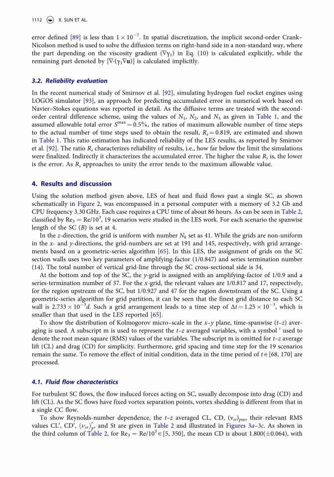
To show Reynolds-number dependence, the t–z averaged CL, CD, (νsr)pm, their relevant RMS values CL0, CD0, ðnsrÞ

0p, and St are given in Table 2 and illustrated in Figures 3a–3c. As shown in

the third column of Table 2, for Re3 ¼ Re/103 ∈ [5, 350], the mean CD is about 1.800(�0.064), with

1112 X. SUN ET AL.

maximum relative deviation of 3.56%. This indicates that in the range of Re3 ∈ [5, 350], drag coef-ficient is Reynolds-number independent. For Re3 ∈ [1, 50], with the increase of Reynolds number, the mean CD increases gradually from 1.543 to 1.804. As indicated in the second column of Table 2, the mean CD is approximately zero. The Reynolds-number dependence of mean CD and CL is also shown in Figure 3a.

The Re dependence of relevant RMS values CL0, CD0, and ðnsrÞ0p can be found from the fifth, sixth,

and seventh columns of Table 2. The sub-grid viscosity is calculated from Eq. (1). Corresponding to the values given by the fifth and sixth columns of Table 2, the CL0 and CD0 are shown as functions of Re3, as shown in Figure 3b. For Re3 ∈ [5, 350], CL0 is about 0.17(�0.0117) with a maximum relative deviation of 6.88%; CD0 is around 0.1(�0.0219).

It can be seen that values of the mean CD and its RMS values agree well with existing experimental data of Luo et al. [14] and LES results of Sohankar [34], although the RMS value of CL is less well predicted. The present LES results indicate that the CL0 value is about twice the CD0 value. Consider-ing the wind tunnel measurement of Tamura and Miyagi [15], the effect of inlet turbulence on aero-dynamic forces on a SC with various corner shapes indicates that the reason of the discrepancy requires further investigation.

The peak value of viscosity ratio (νsr) is sought from the entire computational domain, whose geo-metric parameters are shown in Table 1. As turbulent SC flow involves vortex shedding, the location point of the peak value changes temporally. The mean peak value of viscosity ratio (νsr)pm is based on t-averaging. From Figure 3c, it can be seen that Re dependence of (νsr)pm and its RMS value can be described by the power law, the (νsr)pm and its RMS value increase with Reynolds number, but the growing rate of (νsr)pm is larger. For instance, at Re3 ¼ 125, (νsr)pm is 146.23 with its RMS value of 34.14, as shown in Table 2.

As shown in Table 2, based on lift analysis with discrete Hilbert transform [94], for Re3 ∈ [1, 350], St is 0.1079 for all values of Re, with the power-spectra diagrams for Re3 ¼ 1, 2, …, 250 and 350 given in Figures 4a–4h. This St number is close to the predicted St number of 0.124 for the case of Re ¼ 2.2 � 104 [19], when two-dimensional flow calculation was carried out based on the two-layer (TL) approach with standard k � ε equation with inlet viscosity ratio (rμ ¼ νt/ν) set as 100. As reported by Bosch and Rodi [19], St number measured by Bearman and Trueman [8] was 0.123 for the SC flow at Re ≈ 5 � 104 when the inlet flow turbulence level Tuð¼

ffiffiffiffiffiffiu02pÞ was less than 1.2%.

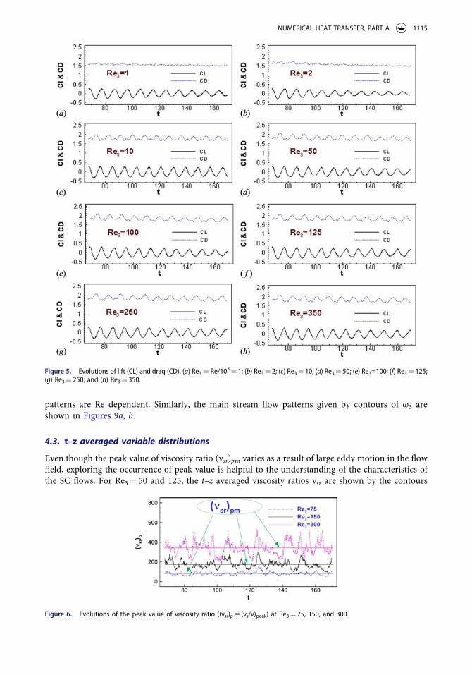
The relevant evolutions of CL and CD at Re3=1, 2, …, and 325 are given in Figures 5a–5h. It can be seen that fluctuation of CD is less than that of CL, which is consistent with the CL0 and CD0 listed in the fifth and sixth columns of Table 2.

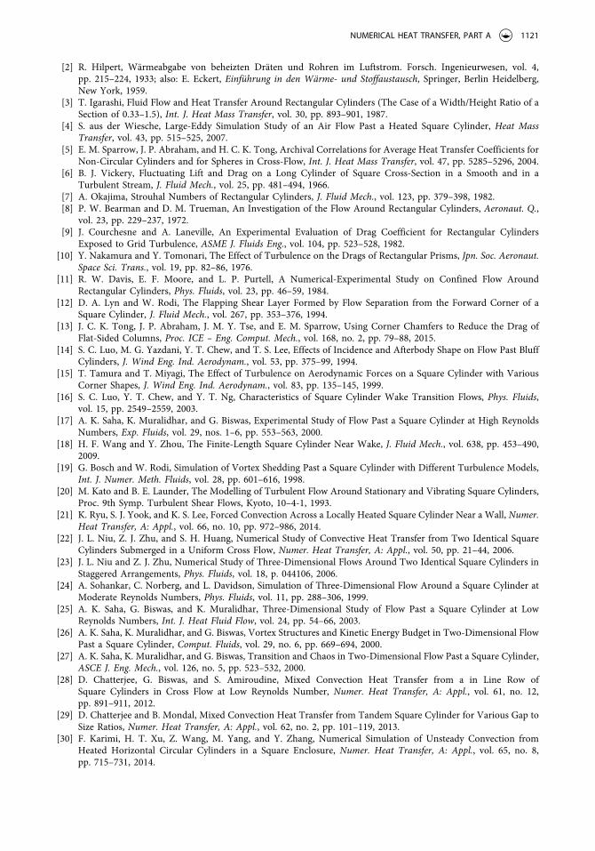
Some properties of the peak value of viscosity ratio can be seen in Figure 6. Both the mean peak value of viscosity ratio (νsr)pm and its RMS value have growing tendency, as shown in Figure 3c. The values of (νsr)pm as shown in Figure 6 are consistent with values shown in Table 2 for Re3 ¼ 75, 150, and 300.

Figure 3. Re dependence of mean lift (CL) and drag (CD) (a), their root mean square (RMS) values of CL and CD (b), and the time- averaged viscosity ratio (νsr)pm as well as its relevant RMS ðnsrÞ

0p (c). Note that (νsr)pm is calculated merely by time-averaging for the

peak value of νsr(¼ νs/ν) in the computational domain, as seen in Figure 6.

NUMERICAL HEAT TRANSFER, PART A 1113

In Table 2, it can be seen that at Re3 ¼ 50, CL0 ¼ 0.1612, and CD0 ¼ 0.0986; while at Re3 ¼ 125, CL0 ¼ 0.1679, and CD0 ¼ 0.1013. In Figures 7a, b, it can be seen that the fluctuation magnitudes of CL and CD are approximately identical for the two cases Re3 ¼ 50, 125.

4.2. Fluid flow patterns

At x ¼ 3, 6, 9, 12 and time t ¼ 170, labeled by values � 0.3, � 0.2, � 0.1, 0, 0.1, 0.2, and 0.3, the contours of streamwise vorticity component ω1 for Re3 ¼ 50 are shown in Figures 8a–8d, with the relevant ω1 contours for Re3 ¼ 125 shown in Figures 8e–8h. A comparison indicates that the secondary flow

Figure 4. Power spectra of the evolutions of CD and CL at (a) Re3 ¼ 1; (b) Re3 ¼ 2; (c) Re3 ¼ 10; (d) Re3 ¼ 50; (e) Re3 ¼ 100; (f) Re3 ¼ 125; (g) Re3 ¼ 250; and (h) Re3 ¼ 350.

1114 X. SUN ET AL.

patterns are Re dependent. Similarly, the main stream flow patterns given by contours of ω3 are shown in Figures 9a, b.

4.3. t–z averaged variable distributions

Even though the peak value of viscosity ratio (νsr)pm varies as a result of large eddy motion in the flow field, exploring the occurrence of peak value is helpful to the understanding of the characteristics of the SC flows. For Re3 ¼ 50 and 125, the t–z averaged viscosity ratios νsr are shown by the contours

Figure 5. Evolutions of lift (CL) and drag (CD). (a) Re3 ¼ Re/103 ¼ 1; (b) Re3 ¼ 2; (c) Re3 ¼ 10; (d) Re3 ¼ 50; (e) Re3=100; (f) Re3 ¼ 125; (g) Re3 ¼ 250; and (h) Re3 ¼ 350.

Figure 6. Evolutions of the peak value of viscosity ratio ((νsr)p � (νs/ν)peak) at Re3 ¼ 75, 150, and 300.

NUMERICAL HEAT TRANSFER, PART A 1115

labeled as 0.05, 1, 5, and 10 in Figures 10a, b. The red colored zone corresponds to the t–z averaged viscosity ratio νsr ≥ 10, the blue colored region corresponds to νsr � 0.05, whereas the yellow, green, and cyan colored regions refer to the ranges of νsr ∈ (5, 10), (1, 5), and (0.05, 1). As shown in Figures 10a, b, for Re3 ¼ 50, and 125, the peak of viscosity ratio occurs in two downstream regions, where the coherent interaction of large eddies is more intense.

For turbulent SC flows, Kolmogorov micro-scale is predicted on the basis of estimating the kinetic energy dissipation rate, similar to previous work [52, 65]. Denoting the Taylor micro-scale as λu [95], we have

k2u ¼ 10nk=e; g2

u ¼ n2=e� �1=2

¼ k2u n e=nð Þ

1=2=ð10 kÞ

h ið24Þ

where k ¼ 12 u02i is the time and z-averaged turbulent kinetic energy, u0i is the instantaneous fluctuation

of velocity component in the xi-direction. While ε is the dissipation rate of k

e ¼ 2nsijsij; sij ¼ ðqu0i=qxj þ qu0j=qxiÞ=2 ð25Þ

with sij being the fluctuation of strain rate of velocity field.

Figure 7. Evolutions of lift (CL) (a) and drag (CD) (b) coefficients at Re3 ¼ 50 and 125.

Figure 8. Contours of streamwise vorticity component (ω1) at t ¼ 170, and four x-locations (i.e., x¼3, 6, 9, and 12) for Re3 ¼ 50 (a–d) and Re3 ¼ 125 (e–h). Note that the contours are labeled by � 0.3, � 0.2, � 0.1, 0, 0.1, 0.2, and 0.3.

1116 X. SUN ET AL.

The t–z averaged field of Kolmogorov micro-scale [log (ηu)] is shown in Figures 11a, b for two Reynolds numbers Re3 ¼ 50 and 125. The t–z averaged Kolmogorov micro-scale [log (ηu)] is less than � 3 for blue colored region, but larger than � 2.7 for red colored region. The yellow, green, and cyan colored regions correspond to log (ηu) ∈ (� 3, � 2.9), (� 2.9, � 2.8), and (� 2.8, � 2.7).

From Figures 11a, b, it can be seen that in the near SC wall regions log (ηu) is less than � 3. With respect to the definition of ηu given by Eq. (24), this property of log (ηu) distribution indicates that near the SC, the dissipation rate of turbulent kinetic energy is larger because of the fluid–solid interaction. From Figures 11a, b, there is an asymmetry of distribution of log (ηu), suggesting that in the SC flow the vortex shedding from the two fix points is not equivalent, which may lead to an asymmetrical distribution of k and its dissipation rate ε [96].

4.4. Instantaneous iso-surfaces

The iso-surfaces of FSI at t ¼ 170 in the sub-domain {x ∈ (0, 7), y ∈ (� 2, 3), z ∈ (1, 3)} are shown in Figures 12a, c. As seen in Eq. (2), the iso-surfaces of FSI depend on vortex motion, which can be quantified by swirling-strength λci [69–71]. The FSI has a laminated structure involving vortex shedding, in addition to those relatively small vortex structures in the SC wake. The distribution of FSI iso-surfaces is Re dependent, since the FSI iso-surfaces as shown in Figure 12a have some differences from those shown by Figure 12c.

The iso-surfaces of viscosity ratio νsr are shown in Figures 12b, d, indicating the reliability of t–z averaged distribution as given in Figures 11a, b.

Figure 9. Contours of spanwise vorticity component (ω3) at t ¼ 170 and z ¼ 2 for Re3 ¼ 50 (a) and Re3=125 (b). Note that contours of ω3 are labeled by � 2, � 1, � 0.5, 0, 0.5, 1, and 2.

Figure 10. Contours of the (t–z) averaged sub-grid viscosity ratio (νsr) at Re3 ¼ 50 (a) and 125 (b). Note that the contours of νsr are labeled by 0.05, 1, 5, and 10.

NUMERICAL HEAT TRANSFER, PART A 1117

4.5. Nusselt numbers

The Re dependence of time-face averaged Nusselt numbers and their arithmetic mean are given in Table 3, with the relevant RMS values shown in Table 4. These Nusselt numbers are based on the length scale d, as shown in Figures 13a, b. Figure 13a shows that the frontal face averaged Nusselt number Nuf is rather sensitive to Re, having the largest growing rate. This is mainly caused by the impingement of free flow stream. While the growing rates of bottom, top, and rear face averaged Nusselt numbers, Nub, Nut, and Nur are smaller, and comparable to each other, primarily caused by the SC flows at zero incident angle have fixed separation points. Influenced by the recirculation near the rear face, the RMS value Nu0r is larger than other RMS values, see in Table 4 or Figure 13b.

Following the comparison approach of Wiesche [4], we further choose 2d as the length scale for the arithmetic mean Nusselt number calculation. In comparing, respectively, with empirical correlations of Hilpert [2] and Igarashi [3], the Re dependence of Nu2d and the corresponding relative deviations

Figure 11. Contours of the (t–z) averaged logarithm of Kolmogorov micro-scale to the base of 10 [log(ηu)] at Re3 ¼ 50 (a) and 125 (b). Note that the contours of log(ηu) are labeled by � 3, � 2.9, � 2.8, and � 2.7.

Figure 12. Iso-surfaces of factor of swirling-strength intermittency (FSI) at t ¼ 170 for Re3 ¼ 75 (a) and Re3 ¼ 150 (c); iso-surfaces of sub-grid viscosity ratio (νsr) at t ¼ 170 for Re3 ¼ 75 (b) and Re3=150 (d). Note that the SC is illustrated simply by a yellow cylinder frame; the FSI iso-surfaces are labeled by 0.05, 0.5, and 0.95, with νsr iso-surfaces labeled by 0.05, 1, and 5.

1118 X. SUN ET AL.

Table 3. Re dependence of Nusselt numbers.

Re3 Nub Nut Nuf Nur Nuam

1 4.941 5.180 21.38 2.416 8.477 2 5.709 6.228 30.28 3.454 11.42 2.5 6.068 6.789 34.08 4.155 12.77 5 7.928 9.625 49.52 7.281 18.59 7.5 9.647 11.874 62.09 9.746 23.34 10 11.28 14.02 73.10 12.03 27.61 12.5 12.81 15.98 84.32 14.33 31.86 25 21.31 24.86 130.41 21.97 49.64 50 33.69 40.41 203.15 36.66 78.48 75 46.57 53.87 263.45 53.99 104.47 100 55.98 65.61 309.14 61.68 123.09 125 65.03 79.04 356.69 73.97 143.68 150 72.79 89.86 405.63 85.21 163.37 200 89.45 111.66 508.36 114.43 205.97 250 100.36 127.41 623.69 142.75 248.55 275 107.02 139.74 690.60 162.30 274.91 300 113.17 148.76 764.71 175.91 300.64 325 117.09 154.58 878.87 192.40 335.73 350 118.77 158.32 1134.57 197.64 402.32

aThe arithmetic mean Nusselt number, Num ¼ (Nub þNut þNuf þNur)/4.

Table 4. Re dependence of the RMS values of Nusselt numbers.

Re3 Nu0b Nu0t Nu0f Nu0r Nu0m

1 0.2076 0.3650 0.0868 0.2670 0.1250 2 0.1874 0.4965 0.2407 0.5667 0.2795 2.5 0.1875 0.6016 0.2838 0.7099 0.3802 5 0.3304 0.5897 0.3082 0.8985 0.4657 7.5 0.6190 0.646 0.3962 1.117 0.4568 10 0.9046 0.9851 0.4588 1.383 0.4224 12.5 1.172 1.364 0.583 1.525 0.4680 25 2.136 2.687 1.160 4.029 1.379 50 4.743 5.191 1.881 8.715 3.734 75 7.163 7.541 1.911 13.63 5.486 100 9.488 10.46 2.616 17.33 7.575 125 11.56 12.66 3.04 20.86 8.84 150 13.34 15.66 3.51 25.29 10.16 200 17.61 22.20 4.92 62.71 20.30 250 18.30 42.65 7.18 93.93 32.37 275 19.53 49.19 8.67 113.78 37.85 300 20.07 53.48 12.66 120.66 40.39 325 21.71 55.67 34.69 139.73 47.20 350 25.66 60.95 65.24 147.66 50.02

Figure 13. Re dependence of Nusselt numbers and their RMS values. Note that here d is used as the length scale to define these Nusselt numbers.

NUMERICAL HEAT TRANSFER, PART A 1119

(σ1, σ2) are shown in Figures 14a, b. It can be seen that the present LES has predicted the mean Nusselt numbers which are consistent with the empirical correlation obtained by earlier experiments of Hilpert [2].

According to the review of Sparrow et al. [5], the change of length scale is to some extent inappropriate. For the SC wake flows at incident angle, the length scale for Nusselt numbers should be the SC’s sectional side length d. The present LES has predicted the mean Nusselt number in good agreement with the correlation of Hilpert [2]. Igarashi [3] utilized constant heat flux in the wind tunnel measurement, resulting in higher values of mean Nusselt number in comparison with those under isothermal wall temperature [97].

5. Conclusions

A swirling-strength based SGS (SbSGS) model is used in the LES of zero-incident incompressible turbulent flows around a SC with convective heat transfer at Reynolds numbers ranging from 103

to 3.5 � 105. LES is performed by a finite difference method, where Taylor-expansion is used to improve the accuracy of discretization. It reveals the following: 1. For Reynolds numbers in the range of 103 to 3.5 � 105, Strouhal number is 0.1079, independent of

Reynolds number. 2. Mean drag coefficient CD is about 1.800(�0.064) when Re ≥ 5000, with a maximum relative

deviation of 3.56%. 3. The peak value of sub-grid viscosity ratio and its RMS values increase with Reynolds number. The

peak occurs in two regions downstream of the SC, when the coherent interactions of large eddies are more intensive.

4. Kolmogorov micro-scale is less than 10� 3 in the near SC wall region when the Reynolds number is over 7.5 � 104. The larger the Reynolds number, the smaller is the Kolmogorov micro-scale.

5. The time-averaged Nusselt number at the frontal face increases with Re rapidly due to the free flow stream impingement. While the RMS at the rear face is larger than other RMS values.

Funding

This work was supported by the Research Committee of The Hong Kong Polytechnic University (Grant No. G-YL03 and G-YM37) and NSFC (11372303).

References

[1] Z. J. Zhu, Numerical Study of Flows Around Rectangular Cylinders, Ph.D. thesis, Shanghai Jiaotong University, P.R. China, pp. 1–22, 1990 (in Chinese).

Figure 14. Re dependence of Nu2d and the relevant relative deviations σ1 and σ2. Note that σ1 ¼ (Nu2d � Nuexp1)/Nuexp1 � 100%, σ2 ¼ (Nu2d � Nuexp2)/Nuexp2 � 100%, where for Re2d ¼ 2Re, Nuexp1 ¼ 0:085Re0:675

2d in Ref. [2]; Nuexp2 ¼ 0:14Re0:662d in Ref. [3].

1120 X. SUN ET AL.

[2] R. Hilpert, Wärmeabgabe von beheizten Dräten und Rohren im Luftstrom. Forsch. Ingenieurwesen, vol. 4, pp. 215–224, 1933; also: E. Eckert, Einführung in den Wärme- und Stoffaustausch, Springer, Berlin Heidelberg, New York, 1959.

[3] T. Igarashi, Fluid Flow and Heat Transfer Around Rectangular Cylinders (The Case of a Width/Height Ratio of a Section of 0.33–1.5), Int. J. Heat Mass Transfer, vol. 30, pp. 893–901, 1987.

[4] S. aus der Wiesche, Large-Eddy Simulation Study of an Air Flow Past a Heated Square Cylinder, Heat Mass Transfer, vol. 43, pp. 515–525, 2007.

[5] E. M. Sparrow, J. P. Abraham, and H. C. K. Tong, Archival Correlations for Average Heat Transfer Coefficients for Non-Circular Cylinders and for Spheres in Cross-Flow, Int. J. Heat Mass Transfer, vol. 47, pp. 5285–5296, 2004.

[6] B. J. Vickery, Fluctuating Lift and Drag on a Long Cylinder of Square Cross-Section in a Smooth and in a Turbulent Stream, J. Fluid Mech., vol. 25, pp. 481–494, 1966.

[7] A. Okajima, Strouhal Numbers of Rectangular Cylinders, J. Fluid Mech., vol. 123, pp. 379–398, 1982. [8] P. W. Bearman and D. M. Trueman, An Investigation of the Flow Around Rectangular Cylinders, Aeronaut. Q.,

vol. 23, pp. 229–237, 1972. [9] J. Courchesne and A. Laneville, An Experimental Evaluation of Drag Coefficient for Rectangular Cylinders

Exposed to Grid Turbulence, ASME J. Fluids Eng., vol. 104, pp. 523–528, 1982. [10] Y. Nakamura and Y. Tomonari, The Effect of Turbulence on the Drags of Rectangular Prisms, Jpn. Soc. Aeronaut.

Space Sci. Trans., vol. 19, pp. 82–86, 1976. [11] R. W. Davis, E. F. Moore, and L. P. Purtell, A Numerical-Experimental Study on Confined Flow Around

Rectangular Cylinders, Phys. Fluids, vol. 23, pp. 46–59, 1984. [12] D. A. Lyn and W. Rodi, The Flapping Shear Layer Formed by Flow Separation from the Forward Corner of a

Square Cylinder, J. Fluid Mech., vol. 267, pp. 353–376, 1994. [13] J. C. K. Tong, J. P. Abraham, J. M. Y. Tse, and E. M. Sparrow, Using Corner Chamfers to Reduce the Drag of

Flat-Sided Columns, Proc. ICE – Eng. Comput. Mech., vol. 168, no. 2, pp. 79–88, 2015. [14] S. C. Luo, M. G. Yazdani, Y. T. Chew, and T. S. Lee, Effects of Incidence and Afterbody Shape on Flow Past Bluff

Cylinders, J. Wind Eng. Ind. Aerodynam., vol. 53, pp. 375–99, 1994. [15] T. Tamura and T. Miyagi, The Effect of Turbulence on Aerodynamic Forces on a Square Cylinder with Various

Corner Shapes, J. Wind Eng. Ind. Aerodynam., vol. 83, pp. 135–145, 1999. [16] S. C. Luo, Y. T. Chew, and Y. T. Ng, Characteristics of Square Cylinder Wake Transition Flows, Phys. Fluids,

vol. 15, pp. 2549–2559, 2003. [17] A. K. Saha, K. Muralidhar, and G. Biswas, Experimental Study of Flow Past a Square Cylinder at High Reynolds

Numbers, Exp. Fluids, vol. 29, nos. 1–6, pp. 553–563, 2000. [18] H. F. Wang and Y. Zhou, The Finite-Length Square Cylinder Near Wake, J. Fluid Mech., vol. 638, pp. 453–490,

2009. [19] G. Bosch and W. Rodi, Simulation of Vortex Shedding Past a Square Cylinder with Different Turbulence Models,

Int. J. Numer. Meth. Fluids, vol. 28, pp. 601–616, 1998. [20] M. Kato and B. E. Launder, The Modelling of Turbulent Flow Around Stationary and Vibrating Square Cylinders,

Proc. 9th Symp. Turbulent Shear Flows, Kyoto, 10–4-1, 1993. [21] K. Ryu, S. J. Yook, and K. S. Lee, Forced Convection Across a Locally Heated Square Cylinder Near a Wall, Numer.

Heat Transfer, A: Appl., vol. 66, no. 10, pp. 972–986, 2014. [22] J. L. Niu, Z. J. Zhu, and S. H. Huang, Numerical Study of Convective Heat Transfer from Two Identical Square

Cylinders Submerged in a Uniform Cross Flow, Numer. Heat Transfer, A: Appl., vol. 50, pp. 21–44, 2006. [23] J. L. Niu and Z. J. Zhu, Numerical Study of Three-Dimensional Flows Around Two Identical Square Cylinders in

Staggered Arrangements, Phys. Fluids, vol. 18, p. 044106, 2006. [24] A. Sohankar, C. Norberg, and L. Davidson, Simulation of Three-Dimensional Flow Around a Square Cylinder at

Moderate Reynolds Numbers, Phys. Fluids, vol. 11, pp. 288–306, 1999. [25] A. K. Saha, G. Biswas, and K. Muralidhar, Three-Dimensional Study of Flow Past a Square Cylinder at Low

Reynolds Numbers, Int. J. Heat Fluid Flow, vol. 24, pp. 54–66, 2003. [26] A. K. Saha, K. Muralidhar, and G. Biswas, Vortex Structures and Kinetic Energy Budget in Two-Dimensional Flow

Past a Square Cylinder, Comput. Fluids, vol. 29, no. 6, pp. 669–694, 2000. [27] A. K. Saha, K. Muralidhar, and G. Biswas, Transition and Chaos in Two-Dimensional Flow Past a Square Cylinder,

ASCE J. Eng. Mech., vol. 126, no. 5, pp. 523–532, 2000. [28] D. Chatterjee, G. Biswas, and S. Amiroudine, Mixed Convection Heat Transfer from a in Line Row of

Square Cylinders in Cross Flow at Low Reynolds Number, Numer. Heat Transfer, A: Appl., vol. 61, no. 12, pp. 891–911, 2012.

[29] D. Chatterjee and B. Mondal, Mixed Convection Heat Transfer from Tandem Square Cylinder for Various Gap to Size Ratios, Numer. Heat Transfer, A: Appl., vol. 62, no. 2, pp. 101–119, 2013.

[30] F. Karimi, H. T. Xu, Z. Wang, M. Yang, and Y. Zhang, Numerical Simulation of Unsteady Convection from Heated Horizontal Circular Cylinders in a Square Enclosure, Numer. Heat Transfer, A: Appl., vol. 65, no. 8, pp. 715–731, 2014.

NUMERICAL HEAT TRANSFER, PART A 1121

[31] D. Chatterjee and S. K. Gupta, Convective Transport Around a Rotating Square Cylinder at Moderate Reynolds Numbers, Numer. Heat Transfer, A: Appl., vol. 67, no. 12, pp. 1386–1407, 2015.

[32] D. Chatterjee and S. K. Gupta, Convective Transport Around Rows of Square Cylinders in Staggered Fashion at Moderate Reynolds Numbers, Numer. Heat Transfer, A: Appl., vol. 68, no. 4, pp. 388–410, 2015.

[33] S. Krajnovic and L. Davidson, Large Eddy Simulation of the Flow Around a Bluff Body, AIAA J., vol. 40, no. 5, pp. 927–936, 2002.

[34] A. Sohankar, Flow over a Bluff Body from Moderate to High Reynolds Numbers using Large Eddy Simulation, Comput. Fluids, vol. 35, pp. 1154–1168, 2006.

[35] K. Hanjalic, One-Point Closure Model for Buoyancy-Driven Turbulent Flows, Annu. Rev. Fluid Mech., vol. 34, pp. 321–347, 2002.

[36] N. N. Smirnov and V. F. Nikitin, Modeling and Simulation of Hydrogen Combustion in Engines, Int. J. Hydrogen Energy, vol. 112, pp. 1122–1136, 2014.

[37] P. Holmes, J. L. Lumley, and G. Berkooz, Turbulence, Coherent Structures, Dynamical Systems and Symmetry, Cambridge University Press, Cambridge, 1996.

[38] J. S. Smagorinsky, Gesneral Circulation Experiments with the Primitive Equations, the Basic Experiment, Mon. Weather Rev., vol. 91, no. 3, pp. 99–164, 1963.

[39] P. Moin and J. Kim, Numerical Investigation of Turbulent Channel Flow, J. Fluid Mech., vol. 118, pp. 341–377, 1982.

[40] M. S. Vázquez and O. Métais, Large-Eddy Simulation of the Turbulent Flow through a Heated Square Duct, J. Fluid Mech., vol. 453, pp. 201–238, 2002.

[41] O. Métais and M. Lesieur, New Tren in Large Eddy Simulation of Turbulence, Annu. Rev. Fluid Mech., vol. 28, pp. 45–82, 1996.

[42] J. Pallares and L. Davidson, Large-Eddy Simulations of Turbulent Flow in a Rotating Square Duct, Phys. Fluids, vol. 12, pp. 2878–2894, 2000.

[43] K. F. Yu, K. S. Lau, and C. K. Chan, Large Eddy Simulation of Particle-Laden Turbulent Flow over a Backward- Facing Step, Commun. Nonlinear Sci. Numer. Simul., vol. 9, no. 2, pp. 251–262, 2004.

[44] Y. C. Guo, P. Jiang, C. K. Chan, and W. Y. Lin, Large Eddy Simulation of Coherent Structures in Rectangular Methane Non-Premixed Flame, J. Comput. Appl. Math., vol. 235, no. 13, pp. 3760–3767, 2011.

[45] C. Duwig, K. J. Nogenmyr, C. K. Chan, and M. Dunn, Large Eddy Simulations of a Piloted Lean Premixed Jet Flame using Finite-Rate Chemistry, Combust., Theory Modell., vol. 15, no. 4, pp. 537–568, 2011.

[46] Y. Y. Wu, C. K. Chan, and L. X. Zhou, Large Eddy Simulation of an Ethylene-Air Turbulent Premixed v-Flame, J. Comput. Appl. Math., vol. 235, no. 13, pp. 3768–3774, 2011.

[47] M. Germano, U. Piomelli, P. Moin, and W. H. Cabot, A Dynamic Subgrid-Scale Eddy Viscosity Model, Phys. Fluids A, vol. 3, no. 7, pp. 1760–1765, 1991.

[48] D. K. Lilly, A Proposed Modification of the Germano Subgrid-Scale Closure Model, Phys. Fluids A, vol. 4, no. 3, pp. 633–635, 1992.

[49] G. X. Cui, C. X. Xu, and Z. S. Zhang, Progress in Large Eddy Simulation of Turbulent Flows, Acta Aerodynam. Sin., vol. 22, no. 2, pp. 121–129, 2004 (in Chinese).

[50] G. X. Cui, H. B. Zhou, Z. S. Zhang, and L. Shao, A New Subgrid Eddy Viscosity Model and Its Application, Chin. J. Comput. Phys., vol. 21, no. 3, pp. 289–293, 2004 (in Chinese).

[51] A. W. Vreman, An Eddy-Viscosity Subgrid-Scale Model for Turbulent Shear Flow: Algebraic Theory and Applications, Phys. Fluids, vol. 16, no. 10, pp. 3670–3681, 2004.

[52] Z. J. Zhu, H. X. Yang, and T. Y. Chen, Numerical Study of Turbulent Heat and Fluid Flow in a Straight Square Duct at Higher Reynolds Numbers, Int. J. Heat Mass Transfer, vol. 53, pp. 356–364, 2010.

[53] F. Nicoud, H. B. Toda, O. Cabrit, S. Bose, and J. Lee, Using Singular Values to Build a Subgrid-Scale Model for Large Eddy Simulations, Phys. Fluids, vol. 23, p. 085106, 2011.

[54] A. Verma and K. Mahesh, A Lagrangian Subgrid-Scale Model with Dynamic Estimation of Lagrangian Time Scale for Large Eddy Simulation of Complex Flows, Phys. Fluids, vol. 24, p. 085101, 2012.

[55] D. D. Holm, Fluctuation Effects on 3d Lagrangian Mean and Eulerian Mean Fluid Motion, Phys. D, vol. 133, nos. 1–4, pp. 215–269, 1999.

[56] A. Cheskidov, D. D. Holm, E. Olson, and E. S. Titi, On a Leray- Model of Turbulence, Proc. Roy. Soc. Lond. A, vol. 461, no. 2055, pp. 629–649, 2005.

[57] B. J. Geurts and D. D. Holm, Regularization Modeling for Large-Eddy Simulation, Phys. Fluids, vol. 15, pp. L13–L16, 2003.

[58] M. van Reeuwijk, H. J. J. Jonker, and K. Hanjalic, Wind and Boundary Layers in Rayleigh Bernard Convection. I. Analysis and Modelling, Phys. Rev. E, vol. 77, p. 036311, 2008.

[59] M. van Reeuwijk, H. J. J. Jonker, and K. Hanjalic, Leray- Simulations of Wall-Bounded Turbulent Flows, Int. J. Heat Fluid Flow, vol. 30, pp. 1044–1053, 2009.

[60] E. Tadmor, Convergence of Spectral Methods for Nonlinear Conservation Laws, SIAM J. Numer. Anal., vol. 26, pp. 1–30, 1989.

1122 X. SUN ET AL.

[61] G. Karamanos and G. E. Karniadakis, A Spectral Vanishing Viscosity Method for Large-Eddy Simulations, J. Comput. Phys., vol. 163, pp. 22–50, 2000.

[62] R. Pasquetti, Spectral Vanishing Viscosity Method for Large-Eddy Simulation of Turbulent Flows, J. Sci. Comput., vol. 27, pp. 365–375, 2006.

[63] E. Lamballais, V. Fortuné, and S. Laizet, Straightforward High-Order Numerical Dissipation via the Viscous Term for Direct and Large Eddy Simulation, J. Comput. Phys., vol. 230, pp. 3270–3275, 2011.

[64] T. Dairay, V. Fortuné, E. Lamballais, and L. E. Brizzi, LES of a Turbulent Jet Impinging on a Heated Wall using High-Order Numerical Schemes, Int. J. Heat Fluid Flow, vol. 50, pp. 177–187, 2014.

[65] Z. J. Zhu, J. L. Niu, and Y. L. Li, Swirling-Strength based Large Eddy Simulation of Turbulent Flows Around Single Square Cylinder at Low Reynolds Numbers, Appl. Math. Mech. Engl. Ed., vol. 35, pp. 959–978, 2014.

[66] Z. Zhang, W. Chen, Z. J. Zhu, and Y. L. Li, Numerical Exploration of Turbulent Natural-Convection in a DASC (i.e., Differentially-Heated Air-Filled Square Cavity) at Ra ¼ 5.33�109, Heat Mass Transfer, vol. 50, pp. 1737–1749, 2014.

[67] N. Uddin, S. O. Neumann, B. Weigand, and B. A. Younis, Large Eddy Simulation and Heat Flux Modeling in a Turbulent Impinging Jet, Numer. Heat Transfer, A: Appl., vol. 55, pp. 906–930, 2009.

[68] S. Chandrasekhar, Hydrodynamic and Hydromagnetic Stability, Chap. III, Oxford University Press, Cambridge, 1961.

[69] J. Zhou, R. J. Adrian, S. Balachandar, and T. M. Kendall, Mechanisms of Generating Coherent Packets of Hairpin Vortices in Channel Flow, J. Fluid Mech., vol. 387, pp. 353–396, 1999.

[70] B. Ganapathisubramani, E. K. Longmire, and I. Marusic, Experimental Investigation of Vortex Properties in a Turbulent Boundary Layer, Phys. Fluids, vol. 18, p. 155105, 2006.

[71] C. T. Lin and Z. J. Zhu, Direct Numerical Simulation of Incompressible Flows in a Zero-Pressure Gradient Turbulent Boundary Layer, Adv. Appl. Math. Mech., vol. 2, pp. 503–517, 2010.

[72] D. K. Lilly, The Representation of Small-Scale Turbulence in Numerical Simulation Experiments, in H. H. Goldstine (ed.), Proc. of IBM Scientific Computing Symposium on Environmental Sciences, Yorktown Heights, New York, pp. 195–210, 1967.

[73] I. Orlanski, A Simple Boundary Condition for Unbounded Flows, J. Comput. Phys., vol. 21, pp. 251–269, 1976.

[74] H. X. Yang, T. Y. Chen, and Z. J. Zhu, Numerical Study of Forced Turbulent Heat Convection in a Straight Square Duct, Int. J. Heat Mass Transfer, vol. 52, pp. 3128–3136, 2009.

[75] W. Q. Tao, Numerical Heat Transfer, Xi’an Jiantong University Press, P.R. China, pp. 195–251, 2001 (in Chinese). [76] S. V. Patankar, Numerical Heat Transfer and Fluid Flow, Hemisphere, New York, 1980. [77] F. H. Harlow and J. E. Welch, Numerical Calculation of Time Dependent Viscous Incompressible flow of Fluid

with Free Surfaces, Phys. Fluids, vol. 8, pp. 2182–2188, 1965. [78] G. Groetzbach, Direct Numerical Simulation of Laminar and Turbulent Benard Convection, J. Fluid Mech.,

vol. 119, pp. 27–53, 1982. [79] M. Manhart, A Zonal Grid Algorithm for DNS of Turbulent Boundary Layers, Comput. Fluids, vol. 33,

pp. 435–461, 2004. [80] K. Khanafer, K. Vafai, and M. Lightstone, Mixed Convection Heat Transfer in Two Dimensional Open-Ended

Enclosures, Int. J. Heat Mass Transfer, vol. 45, pp. 5171–5190, 2002. [81] E. Papanicolaou and Y. Jaluria, Transition to a Periodic Regime in Mixed Convection in a Square Cavity, J. Fluid

Mech., vol. 239, pp. 489–509, 1992. [82] N. Nikitin, Finite-Difference Method for Incompressible Navier-Stokes Equations in Arbitrary Orthogonal

Curvilinear Coordinates, J. Comput. Phys., vol. 217, pp. 759–781, 2006. [83] M. J. Ni and M. A. Abdou, A Bridge between Projection Methods and Simple Type Methods for Incompressible

Navier-Stokes Equations, Int. J. Numer. Meth. Eng., vol. 72, pp. 1490–1512, 2007. [84] Z. F. Tian, X. Liang, and P. X. Yu, A Higher Order Compact Finite Difference Algorithm for Solving the Incompressible

Navier-Stokes Equations, Int. J. Numer. Meth. Eng., vol. 88, pp. 511–532, 2011. [85] M. ElAbdallaoui, M. Hasnaoui, and A. Amahmid, Lattice-Bolzmann Modeling of Natural Convection between a

Square Outer Cylinder, and an Inner Isoscales Triangular Heating Body, Numer. Heat Transfer, A: Appl., vol. 66, no. 9, pp. 1076–1096, 2014.

[86] Z. Wang, Z. Huang, W. Zhang, and G. Xi, A Multidomain Chebyshev Pseudo-Spectral Method for Fluid Flow, and Heat Transfer from Square Cylinders, Numer. Heat Transfer, B: Fundam., vol. 68, no. 3, pp. 224–238, 2015.

[87] F. X. Trias, A. Gorobets, and A. Oliva, A Simple Approach to Discretize the Viscous Terms with Spatially Varying (Eddy-) Viscosity, J. Comput. Phys., vol. 253, pp. 405–417, 2013.

[88] D. L. Brown, R. Cortez, and M. L. Minion, Accurate Projection Methods for the Incompressible Navier-Stokes Equations, J. Comput. Phys., vol. 168, pp. 464–499, 2001.

[89] Z. J. Zhu and H. X. Yang, Numerical Investigation of Transient Laminar Natural Convection of Air in a Tall Cavity, Heat Mass Transfer, vol. 39, pp. 579–587, 2003.

[90] T. J. Baker, Potential Flow Calculation by the Approximate Factorization Method, J. Comput. Phys., vol. 42, pp. 1–19, 1981.

NUMERICAL HEAT TRANSFER, PART A 1123

[91] H. A. Van Der Vorst, BiCGSTAB: A Fast and Smoothly Converging Variant of BICG for the Solution of Non-Symmetric Linear System, SIAM (Soc. Ind. Appl. Math.) J. Sci. Stat. Comput., vol. 13, pp. 631–644, 1992.

[92] N. N. Smirnov, V. B. Betelin, R. M. Shagaliev, V. F. Nikitin, I. M. Belyakov, Yu. N. Deryuguin, S. V. Aksenov, and D. A. Korchazhkin, Hydrogen Fuel Rocket Engines Simulation using LOGOS Code, Int. J. Hydrogen Energy, vol. 39, pp. 10748–10756, 2014.

[93] V. B. Betelin, R. M. Shagaliev, S. V. Aksenov, I. M. Belyakov, Yu. N. Deryuguin, D. A. Korchazhkin, A. S. Kozelkov, V. F. Nikitin, A. V. Sarazov, and D. K. Zelenskiy, Mathematical Simulation of Hydrogen-Oxygen Combustion in Rocket Engines using LOGOS Code, Acta Astronaut., vol. 96, pp. 53–64, 2014.

[94] Z. J. Zhu and H. X. Yang, Discrete Hilbert Transformation and Its Application to Estimate the Wind Speed in Hong Kong, J. Wind Eng. Ind. Aerodynam., vol. 90, pp. 9–18, 2002.

[95] H. Tennekes and J. L. Lumley, A First Course in Turbulence, MIT Press, Cambridge, pp. 146–195, 1974. [96] U. Frisch, The Legacy of A. N. Kolmogorov, in Turbulence, Cambridge University Press, pp. 81–88, 1995. [97] M. Mihiev, Fundamentals of Heat Transfer, National-Thermodynamic Publisher, Moscow, Russia, pp. 1–392,

1956 (In Russian).

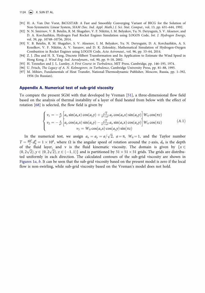
Appendix A. Numerical test of sub-grid viscosity

To compare the present SGM with that developed by Vreman [51], a three-dimensional flow field based on the analysis of thermal instability of a layer of fluid heated from below with the effect of rotation [68] is selected, the flow field is given by

v1 ¼ �pa2 ax sinðaxxÞ cosðayyÞ þ

ffiffiffiTp

p2þa2 ay cosðaxxÞ sinðayyÞh i

W0 cosðpzÞ

v2 ¼ �pa2 ay cosðaxxÞ sinðayyÞ �

ffiffiffiTp

p2þa2 ax sinðaxxÞ cosðayyÞh i

W0 cosðpzÞv3 ¼W0 cosðaxxÞ cosðayyÞ sinðpzÞ

8>><

>>:

ðA:1Þ

In the numerical test, we assign ax ¼ ay ¼ a=ffiffiffi2p

, a ¼ π, W0 ¼ 1, and the Taylor number T ¼ 4X2

nd4

0 ¼ 1� 106, where Ω is the angular speed of rotation around the z-axis, d0 is the depth of the fluid layer, and ν is the fluid kinematic viscosity. The domain is given by x 2fð0; 2

ffiffiffi2pÞ; y 2 ð0; 2

ffiffiffi2pÞ; z 2 ð� 1; 1Þg and is partitioned by 51 � 51 � 51 grids. The grids are distribu-

ted uniformly in each direction. The calculated contours of the sub-grid viscosity are shown in Figures 1a, b. It can be seen that the sub-grid viscosity based on the present model is zero if the local flow is non-swirling, while sub-grid viscosity based on the Vreman’s model does not hold.

1124 X. SUN ET AL.