Computational Challenges of Viscous Incompressible Flows ...
LECTURES
in
COMPUTATIONAL FLUID DYNAMICS
of
INCOMPRESSIBLE FLOW:
Mathematics, Algorithms and Implementations
J. M. McDonough
Departments of Mechanical Engineering and Mathematics
University of Kentucky
c©1991, 2003, 2007
PROLOGUE
Computational fluid dynamics (CFD) can be traced to the early attempts to numerically solve theEuler equations in order to predict effects of bomb blast waves following WW II at the beginning of theCold War. In fact, such efforts were prime drivers in the development of digital computers, and whatwould ultimately come to be termed supercomputers. Such work was motivated further by the “SpaceRace” with the (former) Soviet Union, beginning in the late 1950s. The terminology “computational fluiddynamics,” however, was seldom, if ever, used during this early period; moreover, computational facilitieswere so inadequate that it was not until the late 1960s that anything even remotely resembling a modernCFD problem could be attempted.
The first book devoted to CFD was written by Patrick Roache during a year-long visit to the MechanicalEngineering Department of the University of Kentucky during 1970–71, and was published the followingyear [1]. Computing power at that time was still grossly inadequate for what we today would consideruseful calculations, but significant efforts in algorithm development and analysis were underway in manyleading research universities and national laboratories within the U.S., in Europe (especially France, GreatBritain and Sweden) and in the (former) Soviet Union.
Today, at the beginning of the 21st Century, CFD can be viewed as a mature discipline, at least in thesense that it has been universally recognized as essential for engineering analyses associated with transportphenomena, and with regard to the fact that numerous commercial computer codes are now available. Suchcodes can be executed even on PCs for fairly complex fluid flow problems. Despite this, CFD is not alwaysa part of university curricula and, indeed, it is almost never a required component for a degree—primarilybecause faculty whose backgrounds do not include CFD have yet to retire, and consequently badly-neededcurriculum renovations have not been possible.
We have offered elective courses on CFD at both graduate and undergraduate levels for the past 12 yearsat the University of Kentucky, but like most universities we do not have a formal “CFD Program” in place.Such a program should consist of at least one required undergraduate course in which students would learnto employ a well-known commercial CFD package in solving “real-world” engineering problems involvingfluid flow and heat and mass transfer (just has been required in finite-element analysis of structures formany years). Then at least one (but preferably two) graduate classes in computational numerical analysisshould be available—possibly through an applied mathematics program. The CFD graduate curriculum,per se, should consist of at least the following four one-semester courses: i) CFD of incompressible flow,ii) CFD of compressible flow, iii) turbulence modeling and simulation and iv) grid generation. Clearly,a fifth course on computational transport processes and combustion would be very desirable. The twocomputational numerical analysis courses and the first two CFD classes have been taught at the Universityof Kentucky since 1990 with an introduction to grid generation provided in the second of the numericalanalysis classes, an advanced graduate numerical partial differential equations (PDEs) course.
The present lecture notes correspond to the first item of the above list. They are written to emphasizethe mathematics of the Navier–Stokes (N.–S.) equations of incompressible flow and the algorithms thathave been developed over the past 30 years for solving them. This author is thoroughly convinced thatsome background in the mathematics of the N.–S. equations is essential to avoid conducting exhaustivestudies (and expending considerable effort in doing so) when the mathematics of the problem shows thatthe direction being pursued cannot possibly succeed. (We will provide specific examples of this in Chap. 2of these lectures.) Thus, Chap. 1 is devoted to a fairly advanced presentation of the known theory of theN.–S. equations. The main theorems regarding existence, uniqueness and regularity of solutions will bepresented, and put into a computational context, but without proofs. Omission of these (which tend to beextremely technical, mathematically) is for the sake of engineering students, and we will provide essentialreferences from which mathematicians can obtain proofs and other details of the mathematics.
Chapter 2 will be devoted to presentation of a number of basically elementary topics that are specificallyrelated to CFD but yet impact details of the numerical analysis ultimately required to solve the equationsof motion (the N.–S. equations). They are often crucial to the successful implementation of CFD codes,but at the same time they are not actually a part of the mathematical aspects of numerical analysis. Thesetopics include the different forms into which the N.–S. equations might be cast prior to discretization,the various possible “griddings” of the physical domain of the problem that can be used in the contextof finite-difference, finite-element and finite-volume methods, treatment of the so-called “cell Reynoldsnumber problem” and introduction to “checkerboarding” associated with velocity-pressure decoupling. Anunderstanding of these subjects, along with competence in the numerical analysis of PDEs (a prerequisitefor this course) will serve as adequate preparation for analysis and implementation of the algorithms to beintroduced in Chap. 3. Unlike what is done in most treatments of CFD, we will view numerical analysisas an essential tool for doing CFD, but not, per se, part of CFD itself—so it will not be included in theselectures.
In Chap. 3 we present a (nearly) chronological historical development of the main algorithms employedthrough the years for solving the incompressible N.–S. equations, starting with the marker-and-cell methodand continuing through the SIMPLE algorithms and modern projection methods. We remark that this isone of the main features of the current lectures that is not present in usual treatments. In particular, mostCFD courses tend to focus on a single algorithm and proceed to demonstrate its use in various physicalproblems. But at the level of graduate instruction being targeted by this course we feel it is essential toprovide alternative methods. It is said that “those who do not know history are doomed to repeat it,” andone can see from the CFD literature that, repeatedly, approaches that long ago were shown to be ineffectivecontinue to resurface—and they still are ineffective but may appear less so because of tremendous increasesin computing power since the time of their last introduction. This happens because researchers simply arenot aware of earlier attempts with these very “natural” methods. It is this author’s opinion that the placeto prevent such wasted effort is in the classroom—by presenting both “good” and “bad” (and maybe even“ugly”) algorithms so they can be analyzed and compared, leading the student to a comprehensive andfundamental understanding of what will and will not work for solving the incompressible N.–S. equations—and why.
We note at the outset that all details of algorithms will be presented in the context of finite-difference/finite-volume discretizations, and in essentially all cases they will be restricted to two space dimensions. Butthe algorithms, per se, could easily be implemented in a finite-element setting (and in some cases, even forspectral methods). Furthermore, all details and analyses are conceptually easy to transfer to three spacedimensions. The actual construction of working codes, however, is much more tedious in 3D, and studentsare expected to write and debug codes corresponding to various of the algorithms to be presented. So webelieve the 2-D treatment is to be preferred.
As hinted above, this set of lectures is intended to be delivered during a (three-unit) one-semester course(or, essentially equivalently, during a four-unit quarter course) to fairly advanced graduate students whoare expected to have had at least a first course in general graduate numerical analysis, and should also havehad a second course emphasizing numerical PDEs. It is desired to spend as much time as possible focusingon topics that are specific to solution of the incompressible Navier–Stokes equations without having toexpend lecture time on more elementary topics, so these are considered to be prerequisites. Lectures onthese elements of numerical analysis can be obtained over the Internet as pdf files that can be downloadedby visiting the website http://www.engr.uky.edu/∼acfd and following the links to “lecture notes.”.

Contents
1 The Navier–Stokes Equations: a mathematical perspective 1
1.1 Introductory Remarks . . . . . . . . . . . . . . . . . . . . . . . . . . . . . . . . . . . . . . . 1
1.1.1 The Navier–Stokes equations . . . . . . . . . . . . . . . . . . . . . . . . . . . . . . . 1
1.1.2 Brief history of mathematical analyses of the N.–S. equations . . . . . . . . . . . . . 2
1.1.3 Why study mathematics of the N.–S. equations? . . . . . . . . . . . . . . . . . . . . 2
1.2 Some Basic Functional Analysis . . . . . . . . . . . . . . . . . . . . . . . . . . . . . . . . . . 3
1.2.1 Fourier series and Hilbert spaces . . . . . . . . . . . . . . . . . . . . . . . . . . . . . 3
1.2.2 Classical, weak and strong solutions to PDEs . . . . . . . . . . . . . . . . . . . . . . 8
1.2.3 Finite-difference/finite-volume approximations of non-classical solutions . . . . . . . 21
1.3 Existence, Uniqueness and Regularity of N.–S. Solutions . . . . . . . . . . . . . . . . . . . . 26
1.3.1 Function spaces incorporating physics of incompressible flow . . . . . . . . . . . . . 27
1.3.2 The Helmholtz–Leray decomposition and Leray projection . . . . . . . . . . . . . . . 29
1.3.3 Derivation of “mathematical” forms of the Navier–Stokes equations . . . . . . . . . 30
1.3.4 The main well-known N.–S. solution results . . . . . . . . . . . . . . . . . . . . . . . 38
1.4 Summary . . . . . . . . . . . . . . . . . . . . . . . . . . . . . . . . . . . . . . . . . . . . . . 42
2 Special Numerical Difficulties of the Navier–Stokes Equations 45
2.1 Forms of the Navier–Stokes Equations . . . . . . . . . . . . . . . . . . . . . . . . . . . . . . 45
2.1.1 Primitive-variable formulation . . . . . . . . . . . . . . . . . . . . . . . . . . . . . . . 45
2.1.2 Stream function/vorticity formulations . . . . . . . . . . . . . . . . . . . . . . . . . . 47
2.1.3 Velocity/vorticity formulations . . . . . . . . . . . . . . . . . . . . . . . . . . . . . . 48
2.1.4 Further discussions of primitive variables . . . . . . . . . . . . . . . . . . . . . . . . 49
2.2 Pressure-velocity coupling . . . . . . . . . . . . . . . . . . . . . . . . . . . . . . . . . . . . . 51
2.2.1 Types of grid configurations . . . . . . . . . . . . . . . . . . . . . . . . . . . . . . . . 51
2.2.2 Finite-difference/finite-volume discretization of the N.–S. equations . . . . . . . . . . 54
2.3 Treatments for the Cell-Re Problem and Aliasing . . . . . . . . . . . . . . . . . . . . . . . . 76
2.3.1 The cell-Re problem—its definition and treatment . . . . . . . . . . . . . . . . . . . 77
2.3.2 Treatment of effects of aliasing . . . . . . . . . . . . . . . . . . . . . . . . . . . . . . 87
2.4 Summary . . . . . . . . . . . . . . . . . . . . . . . . . . . . . . . . . . . . . . . . . . . . . . 96
3 Solution Algorithms for the N.–S. Equations 99
3.1 The Marker-and-Cell Method . . . . . . . . . . . . . . . . . . . . . . . . . . . . . . . . . . . 99
3.1.1 Momentum equations . . . . . . . . . . . . . . . . . . . . . . . . . . . . . . . . . . . 100
3.1.2 The pressure Poisson equation . . . . . . . . . . . . . . . . . . . . . . . . . . . . . . 100
3.1.3 Implementation near boundaries . . . . . . . . . . . . . . . . . . . . . . . . . . . . . 102
3.1.4 Marker particle trajectories for free surface tracking . . . . . . . . . . . . . . . . . . 103
3.1.5 The MAC algorithm . . . . . . . . . . . . . . . . . . . . . . . . . . . . . . . . . . . . 105
3.2 SOLA Method . . . . . . . . . . . . . . . . . . . . . . . . . . . . . . . . . . . . . . . . . . . 105
3.3 Artificial Compressibility . . . . . . . . . . . . . . . . . . . . . . . . . . . . . . . . . . . . . 108
3.4 Projection Methods . . . . . . . . . . . . . . . . . . . . . . . . . . . . . . . . . . . . . . . . 111
i

ii CONTENTS
3.4.1 Outline of Chorin’s projection method . . . . . . . . . . . . . . . . . . . . . . . . . . 1123.4.2 Analytical construction of a modern projection method . . . . . . . . . . . . . . . . 1123.4.3 Numerical implementation of projection methods . . . . . . . . . . . . . . . . . . . . 1143.4.4 A second-order projection method . . . . . . . . . . . . . . . . . . . . . . . . . . . . 132
3.5 The SIMPLE Algorithms . . . . . . . . . . . . . . . . . . . . . . . . . . . . . . . . . . . . . 1333.5.1 An analytical version of SIMPLE . . . . . . . . . . . . . . . . . . . . . . . . . . . . . 1333.5.2 The discrete SIMPLE algorithm . . . . . . . . . . . . . . . . . . . . . . . . . . . . . 1353.5.3 The SIMPLER algorithm . . . . . . . . . . . . . . . . . . . . . . . . . . . . . . . . . 140
3.6 Summary . . . . . . . . . . . . . . . . . . . . . . . . . . . . . . . . . . . . . . . . . . . . . . 143
References 144

List of Figures
1.1 Comparison of two boundary condition assignments for the Poisson equation. . . . . . . . . 101.2 Step function constructed by applying the characteristic function to a function f . . . . . . . 231.3 C∞
0 δǫ mollification functions for three values of ǫ. . . . . . . . . . . . . . . . . . . . . . . . 24
2.1 Alternative grid structures for solving the 2-D incompressible N.–S. equations; (a) naturalunstaggered, (b) staggered, (c) partially staggered, (d) cell-centered unstaggered and (e)staggered w/ multiple momentum equations. . . . . . . . . . . . . . . . . . . . . . . . . . . 52
2.2 Lid-driven cavity geometry, boundary conditions and streamlines for the viscous, incom-pressible N.–S. equations. . . . . . . . . . . . . . . . . . . . . . . . . . . . . . . . . . . . . . 54
2.3 Basic unstaggered gridding of problem domain. . . . . . . . . . . . . . . . . . . . . . . . . . 562.4 Non-constant grid function satisfying discrete 1-D continuity equation. . . . . . . . . . . . . 612.5 Non-physical grid function satisfying discrete 2-D continuity equation. . . . . . . . . . . . . 622.6 Non-physical checkerboard pressure distribution. . . . . . . . . . . . . . . . . . . . . . . . . 622.7 Staggered grid cell, Ωi,j. . . . . . . . . . . . . . . . . . . . . . . . . . . . . . . . . . . . . . . 642.8 Grid cell (shaded region) for x-momentum equation. . . . . . . . . . . . . . . . . . . . . . . 662.9 Grid cell (shaded region) for y-momentum equation. . . . . . . . . . . . . . . . . . . . . . . 682.10 Grid-cell indexing. . . . . . . . . . . . . . . . . . . . . . . . . . . . . . . . . . . . . . . . . . 702.11 Staggered-grid boundary condition implementation schematic. . . . . . . . . . . . . . . . . . 722.12 Cell-centered, unstaggered grid. . . . . . . . . . . . . . . . . . . . . . . . . . . . . . . . . . . 752.13 Grid point to grid point oscillations caused by cell-Re problem. . . . . . . . . . . . . . . . . 802.14 Dependence of z+ on cell Re. . . . . . . . . . . . . . . . . . . . . . . . . . . . . . . . . . . . 812.15 Under-sampled oscillatory function demonstrating effects of aliasing. . . . . . . . . . . . . . 882.16 Schematic of a discrete mollifier. . . . . . . . . . . . . . . . . . . . . . . . . . . . . . . . . . 912.17 Wavenumber response of Shuman filter for various values of filter parameter. . . . . . . . . 932.18 Shuman filter applied to solution of Burgers’ equation. . . . . . . . . . . . . . . . . . . . . . 95
3.1 Location of averaged velocity components needed for mixed derivative approximations. . . . 1023.2 Near-boundary grid cells for treatment of right-hand side of Eq. (3.9). . . . . . . . . . . . . 1033.3 Introduction of massless marker particles. . . . . . . . . . . . . . . . . . . . . . . . . . . . . 1043.4 Dependent-variable arrangement for δ-form upwind differencing. . . . . . . . . . . . . . . . 122
iii
Chapter 1
The Navier–Stokes Equations: a
mathematical perspective
In this chapter we provide an introduction to the Navier–Stokes equations from a mainly mathematicalpoint of view in order to lay the proper groundwork for the numerical treatments to follow in subsequentchapters. We begin with a very brief discussion of the equations, themselves, reserving details for later,and we provide an outline of the history of the analysis of these equations. But we make no claim asto completeness of this; the intent is merely to indicate the tremendous amount of work that has beendone. We follow this with basic functional analysis relating to the Navier–Stokes equations, including suchkey ideas as “weak” and “strong” solutions. We then state, without proof, the main results concerningexistence, uniqueness and regularity of solutions, and we discuss these in the framework of the numericalprocedures that will be needed to actually produce solutions.
1.1 Introductory Remarks
As indicated above, this section will consist of presenting the Navier-Stokes equations with cursory remarksregarding the physics embodied in them, and a brief outline of the history of their investigation by, mainly,mathematicians. It will conclude with some remarks on why a basic mathematical study of these equationsis important.
1.1.1 The Navier–Stokes equations
The equations of viscous, incompressible fluid flow, known as the Navier–Stokes (N.–S.) equations afterthe Frenchman (Claude Louis Marie Henri Navier) and Englishman (George Gabriel Stokes) who proposedthem in the early to mid 19th Century, can be expressed as
ρDu
Dt= −∇p+ µ∆u + F
B(1.1a)
∇ · u = 0 , (1.1b)
where ρ is density of the fluid (taken to be a known constant); u ≡ (u1, u2, u3)T is the velocity vector
(which we will often write as (u, v,w)T ); p is fluid pressure; µ is viscosity, and FB
is a body force. D/Dtis the substantial derivative expressing the Lagrangian, or total, acceleration of a fluid parcel in terms of aconvenient laboratory-fixed Eulerian reference frame; ∇ is the gradient operator; ∆ is the Laplacian, and∇· is the divergence operator. We remind the reader that the first of these equations (which is a three-component vector equation) is just Newton’s second law of motion applied to a fluid parcel—the left-handside is mass (per unit volume) times acceleration, while the right-hand side is the sum of forces acting onthe fluid element. Equation (1.1b) is simply conservation of mass in the context of constant-density flow.In the sequel we will provide alternative forms of these basic equations.
1

2 CHAPTER 1. THE NAVIER–STOKES EQUATIONS: A MATHEMATICAL PERSPECTIVE
1.1.2 Brief history of mathematical analyses of the N.–S. equations
It is interesting to note that Navier derived Eq. (1.1a) in 1822 on a very fundamental physical basis includingeffects of attraction and repulsion of neighboring molecules, but did not specify the physics embodied inthe coefficient that ultimately came to be taken as viscosity. Indeed, the effects of molecular interactionsmight be viewed as being somehow equivalent to viscosity (they are certainly related to it, but Navier couldnot have known the details of this), but one must not lose sight of the fact that the continuum hypothesis isactually required to make analysis of fluid flow reasonable in the context of any equations less fundamentalthan the Boltzmann equation (in particular, the N.–S. equations). The derivation by Stokes in 1845 wasthe first to explicitly introduce viscosity.
During the 20th Century the N.–S. equations received increasing attention from mathematicians follow-ing the early studies of Leray [2, 3] in the 1930s in which it was proposed that solutions to these equationscould possibly be singular and that this might be associated with turbulence. The work of Leray spurredconsiderable development of 20th Century functional analysis, and it is often claimed that the N.–S. equa-tions are one of two main progenitors of modern 20th Century mathematical analysis—the other beingSchrodinger’s equation of quantum mechanics. Following Leray’s work was the seminal contribution ofLadyzhenskaya [4] (first available in English in 1963) which provided basic direction and results for furtheranalysis of the N.–S. equations. Beginning in the early 1970s numerous works began to appear that led toa rather different, and modern, view of the equations of fluid motion, namely as dynamical systems. Thebest known of these is probably that of Ruelle and Takens [5] in which it is proposed that the N.–S. equa-tions are capable of describing turbulent fluid motion, that such motion is not random but instead chaoticand associated with a strange attractor of the flow of the dynamical system (the N.–S. equations), andfurthermore such behavior must arise after only a small number (possibly as few as three) of bifurcationsof the equations of motion.
It is interesting to note that this view of the N.–S. equations was in a sense foreseen in the numericalwork of Lorenz [6] in 1963 and the early attempts at direct numerical simulation (DNS) of turbulence by,e.g., Orszag and Patterson [7] in the late 1960s and early 70s. It has in recent years provided the contextfor numerous works on the Navier–Stokes equations beginning with Ladyzhenskaya [8, 9], Temam [10]–[12], Constantin and Foias [13] and many others. Recently, there have been a number of new monographspublished on the Navier–Stokes equations. These include the work by Doering and Gibbon [14] and thevery up-to-date volume by Foias et al. [15] that will be used extensively in the present chapter. We highlyrecommend both of these, but especially the latter, to students interested in details of the mathematicsthat will be somewhat diluted in the current lectures.
1.1.3 Why study mathematics of the N.–S. equations?
Before launching into a mathematical discussion of the N.–S. equations that to some may seem a needlesswaste of time at best (and maybe worse, completely useless impractical ramblings) we need to provide arationale for doing so. The first point to be aware of is that in the 21st Century most (probably eventuallyall) analyses of fluid flow will be performed via CFD. Moreover, such analyses will almost always be carriedout using commercial flow codes not written by the user—and possibly (probably, in most cases) not evenunderstood by the user. One of the main goals of these lectures is to provide the reader with sufficientunderstanding of what is likely to be going on “under the hood” in such codes to motivate caution inaccepting computed results as automatically being accurate. At the same time it is hoped that the readerwill also develop an ability to test the validity and accuracy of computed results. It will be apparent as weproceed that a fair amount of mathematical understanding of the N.–S. equations, and the nature of theirsolutions, is required to do this.
Beyond this is the fact, underscored by Eqs. (1.1), that the N.–S. equations comprise a system of PDEsrequiring the user of commercial software to prescribe sufficient data associated with any given physicalsituation to produce a mathematically well-posed problem. Commercial CFD codes tend generally to bequite robust, and they will often produce results even for problems that are not properly posed. These can
1.2. SOME BASIC FUNCTIONAL ANALYSIS 3
range from easily recognized “garbage out” due to “garbage in” to solutions that look “physically correct”but which are wrong in subtle ways. Clearly, the latter are far more dangerous, but in any case it behoovesusers of commercial software to know sufficient mathematics of the N.–S. equations to reliably constructwell-posed problems—and, sometimes what is required to do so can be counter intuitive based on physicsalone.
1.2 Some Basic Functional Analysis
In this section we will introduce some basic notions from fairly advanced mathematics that are essential toanything beyond a superficial understanding of the Navier–Stokes equations. Indeed, as we have alreadyindicated, a not insignificant part of what we will present was developed by mathematicians in theirstudies of these equations. As might be expected, much of this material is difficult, even for students ofmathematics, and as a consequence, we will usually dilute it considerably (but, hopefully, not fatally) inan effort to render it comprehensible to those not especially well trained in modern analysis.
There are numerous key definitions and basic ideas needed for analysis of the N.–S. equations. Theseinclude Fourier series, Hilbert (and Sobolev) spaces, the Galerkin procedure, weak and strong solutions, andvarious notions such as completeness, compactness and convergence. In some cases we will provide preciseand detailed definitions, while in others we may present only the basic concept. As often as possible we willalso discuss characterizations of the idea under consideration in terms of simpler (hopefully, well-known)mathematics—and/or physics—to clarify these principles and to make them seem more natural.
1.2.1 Fourier series and Hilbert spaces
In this subsection we will briefly introduce several topics required for the study of PDEs in general, andthe Navier–Stokes equations in particular, from a modern viewpoint. These will include Fourier series,Hilbert spaces and some basic ideas associated with function spaces, generally.
Fourier Series
We begin by noting that there has long been a tendency, especially among engineers, to believe thatonly periodic functions can be represented by Fourier series. This misconception apparently arises frominsufficient understanding of convergence of series (of functions), and associated with this, the fact thatperiodic functions are often used in constructing Fourier series. Thus, if we demand uniform convergencesome sense could be made of the claim that only periodic functions can be represented. But, indeed, it isnot possible to impose such a stringent requirement; if it were the case that only periodic functions couldbe represented (and only uniform convergence accepted), there would be no modern theory of PDEs.
Recall for a function, say f(x), defined for x ∈ [0, L], that formally its Fourier series is of the form
f(x) =
∞∑
k
akϕk(x) , (1.2)
where ϕk is a complete set of basis functions, and
ak = 〈f, ϕk〉 ≡∫ L
0f(x)ϕk(x) dx . (1.3)
The integral on the right-hand side is a linear functional termed the inner product when f and ϕk are inappropriate function spaces. We will later return to requirements on f for existence of such a representation.At this time we can at least discuss some terminology associated with the above expressions.
First, the notion of basis functions is analogous to that of basis vectors in linear algebra. For example,in the real N -dimensional Euclidean space RN we can construct a basis eiN
i=1 of the form
ei = (0, 0, . . . ,
i︷︸︸︷1 , 0, . . . , 0)T , (1.4)
4 CHAPTER 1. THE NAVIER–STOKES EQUATIONS: A MATHEMATICAL PERSPECTIVE
with all components of the vector being zero except the ith one, which has a value of unity. We can thenrepresent every vector v ∈ RN as
v =N∑
i=1
〈v,ei〉ei , (1.5)
wherev = (v1, v2, . . . , vN )T ,
and 〈v,ei〉 is now just the usual “dot” product of two vectors. (Also note from our choice of the eis that〈v,ei〉 = vi.) We see from this that we can view Eq. (1.2) as an infinite-dimensional version of (1.5) and,correspondingly, the set ϕk is the infinite-dimensional analogue of the basis set with vectors defined asin Eq. (1.4). But care must be exercised in using such interpretations too literally because there is noquestion of convergence regarding the series in (1.5) for any N <∞. But convergence (and, moreover, thespecific type of convergence) is crucial in making sense of Eq. (1.2). Furthermore, in the finite-dimensionalcase of Eq. (1.5) it is easy to construct the basis set and to guarantee that it is a basis, using simple resultsfrom linear algebra. Treatment of the infinite-dimensional case is less straightforward. In this case weneed the idea of completeness. Although we will not give a rigorous definition, we characterize this in thefollowing way: if a countable basis set is complete (for a particular space of functions, i.e., with respectto a specified norm), then any (and thus, every) function in the space can be constructed in terms of thisbasis.
We remark that completeness is especially important in the context of representing solutions to dif-ferential equations. In particular, in any situation in which the solution is not a priori known (and, e.g.,might have to be determined numerically), it is essential that the chosen solution representation include acomplete basis set. Otherwise, a solution might not be obtained at all from the numerical procedure, or ifone is obtained it could be grossly incorrect.
The question of where to find complete basis sets then arises. In the context of Fourier representationsbeing considered at present we simply note without proof (see, e.g., Gustafson [16] for details) that suchfunctions can be obtained as the eigenfunctions of Sturm–Liouville problems of the form
− d
dx
(p(x)
dϕ
dx
)+ q(x)ϕ = λr(x)ϕ , x ∈ [a, b] (1.6a)
Baϕ = Bbϕ = 0 , (1.6b)
where Ba and Bb are boundary operators at the respective endpoints a and b of the interval; p, q and r aregiven functions of x, and λ is an eigenvalue. It is shown in [16] that such problems have solutions consistingof a countable infinity of λks, and associated with these is the countable and complete set of ϕks.
At this point we see, at least in an heuristic sense, how to construct the series in Eq. (1.2). But wehave not yet indicated for what kinds of functions f this might actually be done. To accomplish this wewill need a few basic details regarding what are called Hilbert spaces.
Hilbert Spaces
We have already implied at least a loose relationship between the usual N -dimensional vector spacesof linear algebra and the Fourier representation Eq. (1.2). Here we will make this somewhat more precise.We will first introduce the concept of a function space, in general, and then that of a Hilbert space. Wefollow this with a discussion of the canonical Hilbert space, denoted L2, and relate this directly to Fourierseries. Finally, we extend these notions to Sobolev spaces which, as we will see, are Hilbert spaces withsomewhat “nicer” properties than those of L2 itself—i.e., functions in a Sobolev space are “smoother”(more regular) than those in L2.
First recall that vector spaces possess the linearity property: if v and w are in the vector space S, forexample, RN and a, b ∈ R (or a, b ∈ C), then
av + bw ∈ S .
1.2. SOME BASIC FUNCTIONAL ANALYSIS 5
This implies that S is closed with respect to finite linear combinations of its elements.If we replace the finite-dimensional vectors v and w with functions f and g, both having Fourier
representations of the form Eq. (1.2), closedness still holds (modulo a few technical details), and we havethe beginnings of a function space. But as we have already hinted, because of the infinite basis set,convergence now becomes an issue, and we need tools with which to deal with it. If we consider a sequenceof functions fn(x)∞n=0, and a possible limit function, say f(x), then we need a way to precisely characterizethe heuristic fn → f as n→ ∞. Recall from elementary analysis that if instead of a sequence of functionswe were to consider a sequence of numbers, say an, we would say that an converges to a, denotedan → a, when |a − an| < ǫ ∀ ǫ > 0, but depending on n. Furthermore, we remind the reader that it isoften essential to be able to consider convergence in a slightly different sense, viz., in the sense of Cauchy:|am − an| < ǫ ⇒ an → a. This property does not always hold, but the class of sequences for which itdoes is large, and any space in which convergence in the sense of Cauchy implies convergence (in the usualsense) is said to be complete.
The natural generalization of this to sequences of functions is to replace the absolute value | · | witha norm ‖ · ‖. We will not at the moment specify how ‖ · ‖ is to be calculated (i.e., which norm is tobe used), but however this might be done we expect that ‖f − fn‖ < ǫ would imply fn → f “in somesense.” This provides sufficient machinery for construction of a function space: namely, a function spaceis a complete linear space of functions equipped with a norm. Such spaces are called Banach spaces, andthey possess somewhat less structure than is needed for our analyses of the N.–S. equations. Independentof this observation, however, is the fact that because there are many different norms, we should expectthat the choice of norm is a key part of identifying/characterizing the particular function space. Indeed,for an expression such as ‖f − fn‖ < ǫ to make sense, it must first be true that ‖f − fn‖ exists; i.e., itmust be that ‖f − fn‖ <∞. This leads us to consider some specific examples of norms.
It is worthwhile to first consider a particular vector norm in a finite-dimensional real Euclidean space—the Euclidean length: let v = (v1, v2, . . . , vN )T ; then the Euclidean norm is simply
‖v‖2 =
(N∑
i=1
v2i
)1/2
,
which is recognized as the length of v. (We have used a “2” subscript notation to specifically distinguishthis norm from the infinity of other finite-dimensional p norms defined in an analogous way.) It is alsoeasy to see that the above expression is (the square root of) the vector dot product of v with itself:
‖v‖22 = v · v = 〈v,v〉 ,
the last equality representing the notation to be used herein, and which is often termed a scalar product—ageneralization of inner product. We can see from these last two equations a close relationship betweennorm and inner (dot) product in Euclidean spaces, and a crucial point is that this same relationship holdsfor a whole class of (infinite-dimensional) function spaces known as Hilbert spaces. In particular, a Hilbertspace is any complete normed linear space whose norm is induced by an inner product. Thus, one canthink of Hilbert spaces as Banach spaces with more structure arising from the “geometry” of the innerproduct. (Recall that in finite-dimensional spaces the dot product can be used to define angles; this is truein infinite-dimensional inner product spaces as well.)
As we will see shortly there are many different Hilbert spaces, but we will begin by considering whatis termed the “canonical” Hilbert space denoted L2. L2 is one member of the family of Lp spaces (all therest of which are only Banach spaces) having norms defined by
‖f‖L
p ≡(∫
Ω|f |p dµ
)1/p
, (1.7)
where Ω is a domain (bounded, or unbounded) in, say RN ; | · | denotes, generally, the complex modulus(or, if f is real valued, absolute value), and µ is a “measure” on Ω. We will neither define, nor explicity

6 CHAPTER 1. THE NAVIER–STOKES EQUATIONS: A MATHEMATICAL PERSPECTIVE
use, the notion of measure to any extent in these lectures, despite its extreme importance in intermediateto advanced analysis, in general. For those readers not familiar with the concept, it will be sufficient forpurposes herein to think of measure as being an interval (or subinterval, possibly small), and to associatedµ with the usual differential dx.
The integral in Eq. (1.7) is a Lebesgue integral (hence, the notation Lp) which provides a crucialgeneralization of the Riemann integral from elementary calculus. In light of our earlier discussions wesee that a function f is in the function space Lp(Ω) if and only if ‖f‖
Lp < ∞. In particular, f ∈ L2(Ω)
whenever ‖f‖L
2 <∞, where
‖f‖L
2 ≡(∫
Ω|f |2 dµ
)1/2
. (1.8)
In the sequel we will consider only real-valued functions f , obviating the need for the | · | notation whenconsidering L2 (or any other even-p Lp space). In addition, we will replace the Lebesgue measure µ withintervals contained in Ω and revert to the usual dx notation, even when the integral formally must be ofLebesgue type.
There is an important easily-proven inequality, applicable in any Hilbert space, known as the Cauchy–Schwarz inequality, and expressed in L2(Ω) as
〈f, g〉 ≤ ‖f‖L
2 ‖g‖L
2 ∀ f, g ∈ L2(Ω) . (1.9)
Hence, the inner product of two functions in L2 is bounded by the product of their L2 norms, both of whichare finite. This turns out to be very important in constructing estimates needed for proofs of existence ofsolutions to PDEs, and holds only in Hilbert spaces. We recognize from this that Hilbert spaces are closedunder multiplication of their elements as well as under finite linear combination. A generalization to otherLp spaces, known as Holder’s inequality, is similarly important, but more difficult to employ for technicalreasons, not the least of which is the fact that closure under multiplication no longer holds.
We now have in place the tools needed to return to the question of what classes of functions maybe represented by Fourier series. The basic answer to this is: any function in L2 (or any other Hilbertspace) can be expressed as a Fourier series. (There are other functions that also can be so represented, butdiscussion of this would take us too far from the main topics of these lectures.) There are several relatedheuristic justifications one can provide for this result. First, we recall that for a function f(x) the formalcalculation of its Fourier coefficients is performed with the formula given in Eq. (1.3), repeated here as
ak = 〈f, ϕk〉 ≡∫
Ωf(x)ϕk(x) dx
for all k in a countably-infinite index set, and where in (1.3) Ω = [0, L] was used. We see by comparing thiswith the Cauchy–Schwarz inequality, Eq. (1.9), that if the ϕks are only in L2(Ω), and f is also in L2(Ω),we can guarantee boundedness (and hence, existence) of the ak.
There are two remarks that should be made at this point. First, in typical cases ϕk lies in nicerspaces than simply L2(Ω), and second the preceding observation is not sufficient to guarantee validity ofthe Fourier representation Eq. (1.2) for L2 functions. In particular, existence of the inner products thatproduce the coefficients does not guarantee that they decay sufficiently fast with increasing k to implyconvergence of the Fourier series. The Riemann–Lebesgue lemma (see any text on beginning graduateanalysis), however, provides a suggestion that this must be true; namely, it states that ak → 0 as k → ∞,even with quite weak hypotheses regarding f and ϕk. But the strongest results come from the Rieszrepresentation theorem that can be used to deduce both existence of Fourier coefficients and convergence ofthe resulting series for f ∈ L2(Ω). A yet more elementary way to see this is through the Parseval identitywhich, in the case that the ϕks are orthonormal, gives
‖f‖2
L2
=∞∑
k
|ak|2 .

1.2. SOME BASIC FUNCTIONAL ANALYSIS 7
Thus, for f ∈ L2(Ω), ‖f‖L
2 <∞ ⇒∑∞k |ak|2 <∞, and by orthonormality
∥∥∥∥∥
∞∑
k
akϕk(x)
∥∥∥∥∥
2
L2
=∞∑
k
|ak|2 <∞ .
Consequently, the Fourier series converges in the L2 norm. The texts by Stakgold [17] provide easily-understood discussions of these various concepts.
We emphasize that periodicity of f has never been used in any of these arguments, but we must alsonote that the above expressions do not imply uniform convergence in Ω. We remark here that by nature ofthe Lp spaces, convergence in L2 does not even imply convergence at every point of Ω—in sharp contrastto uniform convergence. This arises because the Lebesgue integral is based on the concept of (Lebesgue)measure, and it is shown in beginning graduate analysis classes that integration over a set of zero measureproduces a null result. In turn, this implies that we can ignore sets of measure zero when performingLebesgue integration; hence, when calculating the L2 norm, we are permitted to delete regions of “badbehavior” if these regions have zero measure. Furthermore, this leads to the widely-used concept “almosteverywhere.” When dealing with Lp spaces one often specifies that a given property (e.g., convergence ofa Fourier series) holds almost everywhere, denoted a.e. This means that the property in question holdseverywhere in the domain under consideration except on a set of measure zero.
For later purposes it is useful to note that functions in L2 are often characterized as having finite energy.This description comes from the fact that, up to scaling, U2 ≡ U · U is kinetic energy of a velocity fieldhaving magnitude U . This notion extends naturally to functions in general, independent of whether theyhave any direct association with actual physics. Hence, Eq. (1.8) could be associated with (the square rootof) the “energy” of the function f , i.e., f2, and this is clearly finite if f ∈ L2.
Sobolev Spaces
In the analysis of PDEs, especially nonlinear ones such as the N.–S. equations, it is often necessary toestimate the magnitude of derivatives of the solution and, morever, to bound these derivatives. In orderto work more conveniently with such estimates it is useful to define additional function spaces in terms ofnorms of derivatives. The Sobolev spaces, comprise one class of such spaces that can be defined for any Lp
space but herein will be associated only with L2.
To obtain a concise definition of these spaces we will introduce some notation. First, let α = (α1, α2, . . . , αd)denote a vector of d non-negative integers, a multi-index, and define |α| ≡ α1 + α2 + · · · + αd. Then wedenote the partial differential operator ∂|α|/∂xα1
1 · · · ∂xαd
d by Dα. We can now define a general Sobolevnorm (associated with L2(Ω)) as
‖f‖H
m(Ω)
≡(〈f, f〉
Hm
(Ω)
)1/2, (1.10)
where
〈f, g〉H
m(Ω)
≡∑
|α|≤m
∫
ΩDαfDαg dx . (1.11)
The Sobolev space, itself, is defined as
Hm(Ω) =f ∈ L2(Ω);Dαf ∈ L2(Ω), |α| ≤ m
. (1.12)
Clearly, when m = 0, Hm = H0 = L2; m = 1 and m = 2 will be the most important cases for thepresent lectures. The first of these implies that not only is f ∈ L2(Ω), but so also is its first derivative,with analogous statements involving the second derivative when m = 2. We remark that these notions andadditional ones (especially the Sobolev inequalities) are essential to the modern theory of PDEs, but wewill not specifically use anything beyond the results listed above in the present lectures.

8 CHAPTER 1. THE NAVIER–STOKES EQUATIONS: A MATHEMATICAL PERSPECTIVE
1.2.2 Classical, weak and strong solutions to PDEs
In this section we will provide considerable detail on some crucial ideas from modern PDE theory associatedwith so-called weak and strong solutions, and we will also note how these differ from the “classical”solutions familiar to engineers and physicists. To do this we will need the concept of a distribution (or“generalized” function), and we will also require an introduction to the Galerkin procedure. We begin bymaking precise what is meant by a “classical” solution to a differential equation to permit making a cleardistinction between this and weak and strong solutions. We then provide an example of a weak solution tomotivate the need for such a concept and follow this with an introduction to distribution theory, leadingto the formal definition of weak solution. Next we show that such solutions can be constructed using theGalerkin procedure, and we conclude the section with a definition of strong solution.
Classical Solutions
It is probably useful at this point to recall some generally-known facts regarding partial differentialequations and their (classical) solutions, both to motivate the need for and to better understand the maintopics of this section, namely weak and strong solutions. We let P(·) denote a general partial differentialoperator, common examples of which are the heat, wave and Laplace operators; P could be abstractnotation for any of these, but also for much more general operators such as the N.–S. operator. To makethe initial treatment more concrete we will take P to be the heat operator:
P( · ) ≡[∂
∂t− κ
∂2
∂x2
]( · ) , (1.13)
where κ > 0 is thermal diffusivity, here taken to be constant.
If we now specify a spatial domain and initial and boundary data we can construct a well-posed problemassociated with this operator. For example, if the spatial domain is Ω = R1, then no boundary conditionsneed be given, and the complete heat equation problem can be expressed as
∂u
∂t= κ
∂2u
∂x2, x ∈ Ω ≡ (−∞,∞) (1.14a)
u(x, 0) = u0(x), x ∈ Ω , (1.14b)
where u0(x) is given initial data.
A classical solution to this problem is one that satisfies Eq. (1.14a) ∀ t > 0, and coincides with u0(x)at t = 0 ∀ x ∈ Ω. For this to be true (assuming such a solution exists) it is necessary that u ∈ C1 withrespect to time, and u ∈ C2 with respect to the spatial coordinate; i.e., u ∈ C1(0,∞)×C2(Ω).
As we noted earlier, a modern view of the N.–S. equations is as a dynamical system, and it is worthwhileto introduce this viewpoint here in the well-understood context of the heat equation. From a non-rigorousviewpoint dynamical system is simply anything that undergoes evolution in time, and it is clear that Eqs.(1.14) fit this description. Because of the emphasis on temporal behavior it is common to express dynamicalsystems in the abstract form
du
dt= F (u) , (1.15a)
u(0) = u0 , (1.15b)
even though F may be a (spatial) partial differential operator, and u thus depends also on spatial coordi-nates.
This leads to a slightly different, but equivalent, view of the solution and corresponding notationassociated with the function spaces of which it is a member. Namely, we can think of Eq. (1.15a) as
1.2. SOME BASIC FUNCTIONAL ANALYSIS 9
abstractly providing a mapping from the space of functions corresponding to the right-hand side, that is,C2(Ω) in the present case, to those of the left-hand side, C1(0,∞), and denote this as
u(t) ∈ C1(0,∞;C2(Ω)) . (1.16)
This notation will be widely used in the sequel, so it is worthwhile to understand what it implies. In words,it says that u(t) is a function that is once continuously differentiable in time on the positive real line, andis obtained as a mapping from the twice continuously differentiable functions in the (spatial) domain Ω.
The final piece of terminology that is readily demonstrated in the context of classical solutions (butwhich applies in general) is that of solution operator. Recall from elementary PDE theory that Eqs. (1.14)have the exact solution
u(x, t) =1√
4πκt
∫ ∞
−∞u0(ξ)e
−(x−ξ)2
4κt dξ ∀ (x, t) ∈ (−∞,∞)×(0,∞) . (1.17)
It is obvious from the form of (1.17) that it is a linear transformation that maps the initial data u0 tothe solution of the PDE at any specified later time, and for all spatial locations of the problem domain Ω.Such a mapping is called a solution operator, and the notation
u(t) = S(t)u0 (1.18)
is widely used. This corresponds to choosing a time t, substituting it into the kernel of the solution operator,e−(x−ξ)2/4κt, and evaluating the integral for all desired spatial locations x. Suppression of the x notation, asin (1.18), can to some extent be related to the dynamical systems viewpoint described above. We remarkthat derivation of (1.17) is elementary, but it is particularly important because its form permits explicitanalysis of regularity (i.e., smoothness) of solutions to the problem and, in particular, determination thatindeed the solution is of sufficient smoothness to be classical in the sense indicated earlier. Such an analysisis provided in Berg and McGregor [18], among many other references.
A Non-Classical Solution
The concept of weak solution is one of the most important in the modern theory of partial differentialequations—basically, the theory could not exist without this idea. It was first introduced by Leray in hisstudies of the Navier–Stokes equations, but we will present it here first in a more general abstract (andhence, simpler) setting and later apply it to the N.–S. equations.
The basic idea underlying the term weak solution is that of a solution to a differential equation that isnot sufficiently regular to permit the differentiations required to substitute the solution into the equation.This lack of smoothness might occur on only small subsets of the domain Ω, or it could be present foressentially all of Ω. In any case, there would be parts of the solution domain on which the solution couldnot be differentiated enough times to satisfy the differential equation in the classical sense.
For those readers who have had no more than a first course in PDEs such ideas may seem rathercounterintuitive, at best. Indeed, most solutions studied in a first course are classical; but not all are.Unfortunately, in a beginning treatment the tools needed for analysis of non-classical solutions (eitherweak or strong) are not available, so no attempts are usually made to address lack of regularity of suchsolutions. Here we will present a simple example to demonstrate that solutions to PDEs need not alwaysbe smooth. This is intended to provide motivation/justification for the discussions of weak and strongsolutions that follow.
We consider Poisson’s equation on the interior of the unit square Ω with Dirichlet conditions prescribedon the boundary of Ω, denoted ∂Ω:
∆u = f , (x, y) ∈ (0, 1)×(0, 1) ≡ Ω , (1.19a)
u(x, y) = g(x, y) , (x, y) ∈ ∂Ω . (1.19b)
10 CHAPTER 1. THE NAVIER–STOKES EQUATIONS: A MATHEMATICAL PERSPECTIVE
The reader can easily check that if
f(x, y) =13
4π2 sinπx sin
3
2πy , ∀ (x, y) ∈ Ω , (1.20)
then the function
u(x, y) = − sinπx sin3
2πy (1.21)
is a solution to the differential equation (1.19a). Clearly this solution is a classical one if the boundaryfunction g satisfies
g(x, y) = u(x, y)∣∣∣∂Ω. (1.22)
That is, g ≡ 0 except at y = 1, where g = sinπx holds.
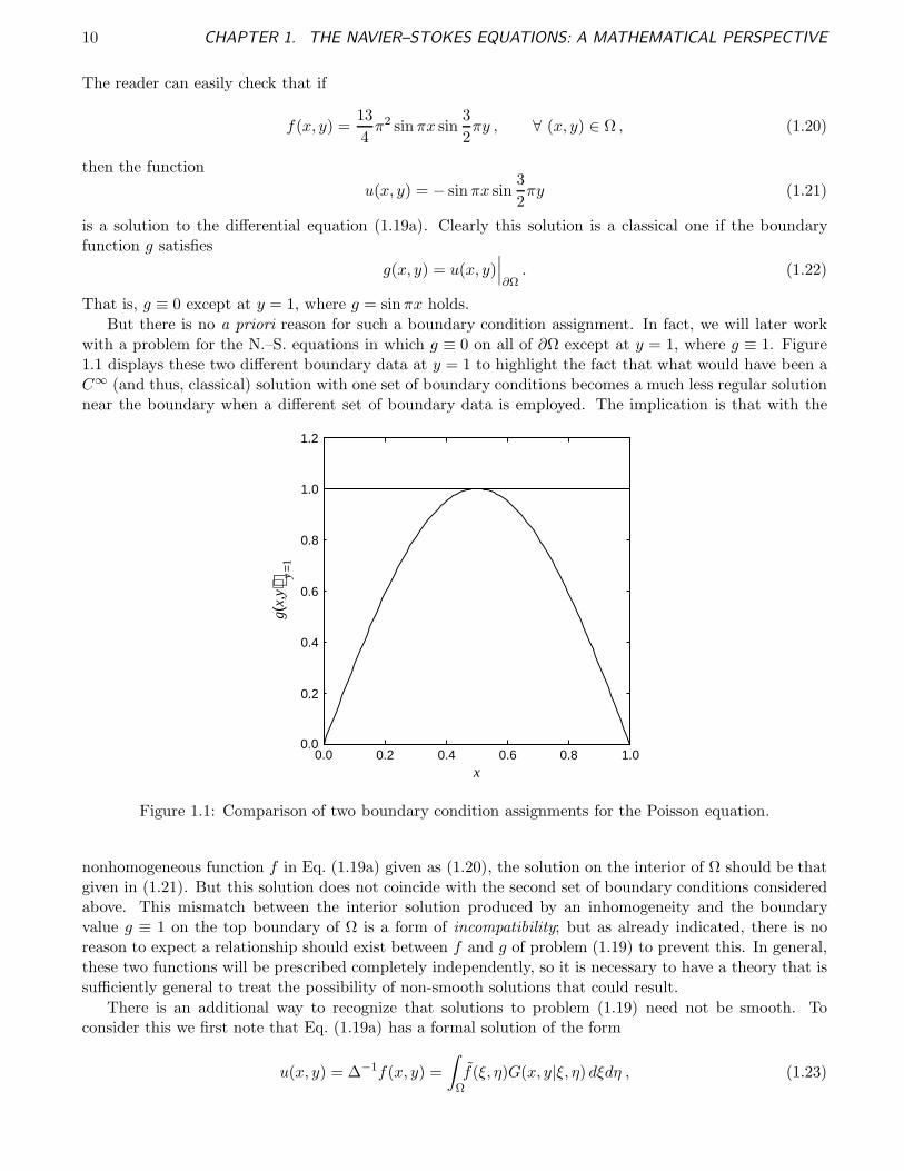
But there is no a priori reason for such a boundary condition assignment. In fact, we will later workwith a problem for the N.–S. equations in which g ≡ 0 on all of ∂Ω except at y = 1, where g ≡ 1. Figure1.1 displays these two different boundary data at y = 1 to highlight the fact that what would have been aC∞ (and thus, classical) solution with one set of boundary conditions becomes a much less regular solutionnear the boundary when a different set of boundary data is employed. The implication is that with the
0
0.2
0.4
0.6
0.8
1
1.2
0 0.2 0.4 0.6 0.8 1
x
g(x,
y) y
=1
1.2
1.0
0.8
0.6
0.4
0.2
0.00.0 0.2 0.4 0.6 0.8 1.0
Figure 1.1: Comparison of two boundary condition assignments for the Poisson equation.
nonhomogeneous function f in Eq. (1.19a) given as (1.20), the solution on the interior of Ω should be thatgiven in (1.21). But this solution does not coincide with the second set of boundary conditions consideredabove. This mismatch between the interior solution produced by an inhomogeneity and the boundaryvalue g ≡ 1 on the top boundary of Ω is a form of incompatibility; but as already indicated, there is noreason to expect a relationship should exist between f and g of problem (1.19) to prevent this. In general,these two functions will be prescribed completely independently, so it is necessary to have a theory that issufficiently general to treat the possibility of non-smooth solutions that could result.
There is an additional way to recognize that solutions to problem (1.19) need not be smooth. Toconsider this we first note that Eq. (1.19a) has a formal solution of the form
u(x, y) = ∆−1f(x, y) =
∫
Ωf(ξ, η)G(x, y|ξ, η) dξdη , (1.23)
1.2. SOME BASIC FUNCTIONAL ANALYSIS 11
where G(· | ·) is the Green’s function for the 2-D Laplacian with (homogeneous) Dirichlet boundary condi-tions (see, e.g., Stakgold [17] for construction of Green’s functions), and f is the original right-hand sidefunction f in Eq. (1.19a) modified to account for transformation of the nonhomogeneous boundary data(1.19b) to the inhomogeneity of the differential equation (see Berg and McGregor [18] for details).
First observe that Eq. (1.23) provides a second example of a solution operator, now acting only oninhomogeneities and boundary data. But the terminology is more widely used in the context of time-dependent problems discussed earlier; in this regard we also note that the kernel of the solution operatorin Eq. (1.17) is often called the causal Green’s function to emphasize the fact that it is associated withtime-dependent behavior.
We next notice that the right-hand side of Eq. (1.23) is in the form of an inner product. Thus, if Gis at least in L2(Ω), the Cauchy–Schwarz inequality guarantees boundedness of this integral and, hence,existence of the solution u to problem (1.19) even if f is no smoother than being in L2(Ω) would imply.Indeed, this guarantees no smoothness at all—not even continuity in the usual sense. For example, it iseasily checked that the function defined by
f(x) =
1 , x irrational
0 , x rational ,
for x ∈ [0, 1] is in L2.Suppose now that f ∈ L2(Ω), but not any smoother. Then we must ask what this implies regarding
regularity of u, the solution to (1.19). From Eq. (1.19a) we see that f ∈ L2(Ω) implies ∆u ∈ L2(Ω), andhence u ∈ H2(Ω); i.e., the second derivatives of u are in L2. Thus, the second derivatives of u exist a.e.,but may not be smooth—hence, it may be the case that no higher derivatives exist. (Recall that evencontinuity of the second derivative would not be sufficient to guarantee existence of the third derivative.)We remark, however, that u ∈ H2 implies existence of ∆u a.e., which characterizes a strong, but notclassical, solution.
Introduction to Distribution Theory
We emphasize at this point that preceding discussion has been heuristic and lacking precision. Inparticular, it is possible that u is not even in H2, implying existence only of what are termed distributional(or weak) derivatives. We will now summarize some key elements from the theory of distributions to allowa more accurate description. We first observe that what is termed a distribution by mathematicians isusually called a “generalized function” by physicists and engineers. Indeed, use of so-called “operationalcalculus” on such functions, especially by engineers in the early 20th Century, preceded by many years therigorous distribution theory of Schwartz [19] that ultimately provided justification for such techniques.
The main difficulty with generalized functions is that they are not functions. Hence, even pointwiseevaluation cannot necessarily be performed, and differentiation is completely meaningless if viewed in theusual sense. We can see this by examining what is probably the best-known generalized function, the Diracδ-function which arises repeatedly in quantum mechanics, but which can also be used to define the Green’sfunction discussed earlier (see, e.g., Stakgold [17] for details). The Dirac δ-function possesses the followingproperties:
i) it is zero on all of R1 except at zero, where its value is infinity;
ii) it has the normalization ∫ ∞
−∞δ(x) dx = 1 ;
iii) it exhibits the “sifting property,”∫ ∞
−∞f(x)δ(x− x0) dx = f(x0) .

12 CHAPTER 1. THE NAVIER–STOKES EQUATIONS: A MATHEMATICAL PERSPECTIVE
It is clear from the first of the above properties that δ(x) cannot be a function in any reasonable sense—itis zero everywhere except at a single point, where it is undefined! But the sifting property turns out tobe valuable. Our main reason for presenting this function here, however, is to introduce a method ofapproximating generalized functions that suggests how they might be interpreted, and at the same timecan sometimes be valuable in its own right.
When applying operational calculus it is often useful to obtain the δ-function by differentiating theHeaviside function, defined as
H(x) =
0 x < 0 ,
1 x ≥ 0 .
Clearly, this function is not continuous at x = 0 and so cannot possibly be differentiable there. So whatsense can be made of the notion that the δ-function is the derivative of the Heaviside function? To answerthis question we employ what is sometimes called a δ-sequence (see Stakgold [17]). The starting point (butnot the one used in [17]) in the present case is the hyperbolic tangent function tanh kx. This function isin C∞(R1) ∀ k <∞, but it is easily seen (at least heuristically) that
1
2
[tanh kx+ 1
]→ H(x)
as k → ∞. Since tanh kx is differentiable (in fact, C∞) we can perform the differentiation and then letk → ∞ to find that we obtain (after appropriate normalization) a function with precisely the properties ofthe δ-function. This suggests that a useful way to define distributions would be in terms of C∞ functions.As we will now show, however, this is not quite as direct as utilizing δ-sequences, but can be made to bevery general.
We begin with some additional notation and terminology. Let C∞0 denote the space of infinitely
continuously differentiable functions having compact support, the latter meaning that such functions vanishoutside a bounded interval. It is common in the theory of generalized functions to term functions of thistype as test functions and denote the space of test functions by D. Next, recall that when we introduced theinner product in Eq. (1.3) we noted that this is in the form of a so-called linear functional. In particular, ifneither f nor ϕk of (1.3) is in L2, then the expression cannot be viewed as an inner product, but instead isa more general scalar product, and in the context of Banach spaces this is (loosely—see below) referred toas a linear functional. It will be convenient to define distributions (generalized functions) in terms of linearfunctionals 〈 · , · 〉 such that one of the two entries comes from the space D of test functions. In particular,as in [17], we state the following.
Definition 1.1 A linear functional on the space D of test functions is a mapping f that assigns to eachtest function ϕ(x) a real number 〈f, ϕ〉 with the property that ∀ a, b ∈ R1 and ∀ ϕ1, ϕ2 ∈ D,
〈f, aϕ1 + bϕ2〉 = a〈f, ϕ1〉 + b〈f, ϕ2〉 . (1.24)
In the present context f need not be a function in the usual sense, and we often apply the term linearfunctional to f itself, rather than to the number 〈f, ϕ〉 that it generates when integrated against a testfunction.
We next define a “weak form of continuity” for linear functionals in the following way. First observethat if ϕ ≡ 0, then 〈f, ϕ〉 = 0 for any f that is finite a.e. on its domain of definition. Now let ϕn denotea sequence of functions in D. Then continuity of a linear functional f is defined as follows.
Definition 1.2 A linear functional f on D is continuous if and only if 〈f, ϕn〉 → 0 whenever ϕn → 0.
Observe that in contrast to the pointwise definition for continuity of functions, continuity of a functionalis defined in terms of an integral and is thus often termed weak continuity. Moreover, a sequence of (test)functions is required to check continuity of a functional. Also note, however, that for each n 〈f, ϕn〉 is a
1.2. SOME BASIC FUNCTIONAL ANALYSIS 13
real number (from the definition of functional), so the test of continuity of a functional is equivalent tochecking convergence (to zero) of a sequence of real numbers. We remark that, conceptually, this is notextremely different from the δ-ǫ definition of continuity in elementary analysis where we must permit δ > 0to be arbitrarily small. Here, we would simply use ‖ϕ‖ < δ with ‖ · ‖ being the uniform norm.
We have now accumulated sufficient information to be able to give a precise meaning to the termdistribution; in particular, we have the following:
Definition 1.3 A distribution is a continuous linear functional on the space D of test functions.
Because of linearity we have not only (1.24), but also that ∀ ϕ ∈ D and a, b ∈ R1 (or in C) we candefine new distributions as linear combinations of other distributions. For example, suppose f1 and f2 aredistributions. Then f ≡ af1 + bf2 is also a distribution for we have
〈f, ϕ〉 = 〈af1 + bf2, ϕ〉 = a〈f1, ϕ〉 + b〈f2, ϕ〉 . (1.25)
Finally, we remark that not all distributions are defined via linear functionals. (Recall that no testfunction was used to define the Dirac δ-function.) More details regarding this can be found in [17], but wenote that for our purposes Def. 1.3 will usually suffice.
From the standpoint of understanding weak solutions to differential equations, the most importantoperation associated with distributions clearly must be differentiation. (There are several other operations,and we refer the reader to [17] for discussions of these.) Indeed, it was specifically the possibility thatsolutions might exist that were not sufficiently differentiable to satisfy the differential equation that hasmotivated these discussions. But because distributions are defined in terms of integrals, we first need tointroduce some terminology associated with these.
Definition 1.4 A function is said to be integrable on R if∫ ∞
−∞|f | dx <∞ . (1.26)
From Eq. (1.7) it is clear that this implies f ∈ L1(R). In the sense of Riemann integration from elementaryanalysis we might say that f is “absolutely integrable.” It is possible, of course, that the integral overR might not exist in the sense of Eq. (1.26), but that integrals over subsets of R might still be finite.Associated with this is the concept of local integrability. We say a function f is locally integrable, denotedhere as L1
loc, if for every finite subset Ω ⊂ R we have∫
Ω|f | dx <∞ , (1.27)
even though integrability in the sense of (1.26) might not hold. We can construct analogous definitionscorresponding to any of the other Lp spaces (and the Hm spaces, as well), but this is not needed for ourimmediate purposes.
We can now state a lemma that is important in constructing derivatives of distributions.
Lemma 1.1 Every locally-integrable function generates a distribution.
This is easily proven since local integrability along with compact support of test functions is sufficientto guarantee (weak) continuity of the associated linear functional.
Now let f be a differentiable function whose derivative f ′ is in L1loc. In addition, let ϕ ∈ D. From the
preceding statement we see that f ′ generates the distribution
〈f ′, ϕ〉 ≡∫ ∞
−∞f ′(x)ϕ(x) dx
= fϕ
∣∣∣∣∞
−∞
−∫ ∞
−∞f(x)ϕ′(x) dx .

14 CHAPTER 1. THE NAVIER–STOKES EQUATIONS: A MATHEMATICAL PERSPECTIVE
But since ϕ ∈ D has compact support, we see that
fϕ
∣∣∣∣∞
−∞
= 0 .
This suggests how we can construct the derivative of a distribution. Namely, now let f be any distri-bution associated with a linear functional, and write
〈f ′, ϕ〉 = −〈f, ϕ′〉 . (1.28)
That is, we have used integration by parts to move (formal) differentiation off of a generally non-differentiabledistribution and onto a C∞
0 test function. Again, the compact support of ϕ removes the need to deal withboundary terms that arise during integration by parts. Furthermore, it is clear that the right-hand side of(1.28) is also a distribution since ϕ′ is also a valid test function.
The derivative calculated in Eq. (1.28) in general possesses no pointwise values. It is termed a distri-butional, or weak, derivative because it is defined only in terms of integration over the support of the testfunction ϕ. We also note that higher distributional derivatives can be calculated via repeated integrationsby parts and satisfy the general formula
〈f (n), ϕ〉 = (−1)n〈f, ϕ(n)〉 (1.29)
for the nth distributional derivative of f , as the reader may easily demonstrate..
An important—and in some sense surprising—observation is that distributions are infinitely differen-tiable in the weak sense, even though they may have no derivatives at all (in fact, might not even becontinuous) in the pointwise sense. This follows from the fact that the test functions, by definition, are inC∞, and it is only these that are actually differentiated when performing distributional differentiation.
Weak Solutions—in General
We now have the tools needed to consider weak solutions to differential equations. There is one addi-tional piece of terminology required for a concise statement, and it furthermore has much wider applicationthan we will utilize herein. It is the (formal) adjoint of a differential operator. We will explicitly consideronly spatial operators, but the basic ideas can be extended to more general cases. Let
L(·) ≡[
n∑
k=0
ak(x)dk
dxk
](·) (1.30)
be a general variable-coefficient nth-order linear operator. Then the formal adjoint of L, denoted L∗, isobtained by forming a linear functional—simply an inner product in Hilbert spaces, integrating by parts,and ignoring boundary terms. This leads to
L∗(·) ≡n∑
k=0
(−1)kdk(ak(x) ·)
dxk., (1.31)
as the reader is encouraged to demonstrate.
Because the adjoint is such an important concept, in general, it is worthwhile to consider constructingone in a specific case.
EXAMPLE 1.1: Consider the second-order linear operator
L = a(x)d2
dx2+ b(x)
d
dx+ c(x) ,
1.2. SOME BASIC FUNCTIONAL ANALYSIS 15
operating on C2 functions that do not necessarily possess compact support. As noted above, we begin byforming the inner product
〈Lu, v〉 =
∫ (a(x)u′′ + b(x)u′ + c(x)u
)v dx
=
∫a(x)u′′v dx+
∫b(x)u′v dx+
∫c(x)uv dx ,
for v also in C2 (and not possessing compact support, in general). Application of integration by parts(twice) to the first integral on the right-hand side of the above produces
∫au′′v = au′v
∣∣∣− u(av)′∣∣∣+∫
(av)′′u .
Similarly, from the second integral we obtain
∫bu′v = buv
∣∣∣−∫
(bv)′u ,
and the third integral remains unchanged.Now disregard the boundary terms, and collect the above results to obtain
〈Lu, v〉 = 〈u, (av)′′〉 − 〈u, (bv)′〉 + 〈u, (cv)〉= 〈u,L∗v〉 ,
with the last line following from the definition/notation of Eq. (1.31).There are three things to note at this point. First, if 〈u, v〉 had been a distribution on v ∈ D, the
the boundary terms would have automatically vanished due to the compact support of v. Second, if theoperator L were part of a boundary-value problem, then the boundary terms arising in the integrations byparts would be used to determine the adjoint boundary conditions for the corresponding adjoint boundary-value problem. In this situation, if it happens that L∗ = L and the adjoint boundary conditions are ofthe same form as those for L, the boundary-value problem is said to be self adjoint. In an abstract sensethis is analogous to symmetry of a matrix, and indeed, the matrices arising from, e.g., finite-difference,discretization of such problems are symmetric. Finally, we note that analogous constructions can be carriedout in higher spatial dimensions.
With this notion of adjoint operators in hand, we can now give a precise definition of weak solution toa differential equation.
Definition 1.5 Let P be a differential operator with formal adjoint P∗, and let f be a distribution. Thena weak solution to the differential equation
Pu = f
is any distribution u that satisfies
〈u,P∗ϕ〉 = 〈f, ϕ〉 ∀ ϕ ∈ D . (1.32)
We remark that while such definitions are extremely important for theoretical purposes, they are of littlepractical (computational) use, in general, with the main exception being finite-element methods based onvariational principles. In particular, this is a global (integral) rather than pointwise result, and it formallymust be tested ∀ ϕ ∈ D. Thus, we need to investigate how weak solutions might be generated via numericaltechniques.
16 CHAPTER 1. THE NAVIER–STOKES EQUATIONS: A MATHEMATICAL PERSPECTIVE
The Galerkin Procedure
The best-known approach to obtaining weak solutions via numerical methods is the Galerkin procedure.This technique is also very important in theoretical analyses, especially for the N.–S. equations, as willbecome evident below. Here we will provide a somewhat general and abstract treatment, and later studythe N.–S. equations as a specific example.
The Galerkin procedure can be formally constructed via the following sequence of steps.
i) Represent each dependent variable and forcing term of the differential equation (DE) as a Fourierseries with basis functions depending on spatial coordinates. (Note: if the DE is not time dependent,the Fourier coefficients are constants; otherwise, they are functions of time.)
ii) Substitute these solution representations into the DE.
iii) Commute differentiation and series summation for each appropriate term, and differentiate the basisfunctions and/or Fourier coefficients, as appropriate.
iv) Form inner products with the DE and every member of the basis set. This will formally result ina countably-infinite system of equations (either algebraic or differential initial-value) for the Fouriercoefficients.
v) Truncate this system to a finite number N , and solve (or analyze—this may be all that is possible innonlinear cases) the result for the Fourier coefficients.
We emphasize that it is merely the Fourier coefficients that are to be determined from any suchnumerical procedure, and once these are found they can be substituted into the solution representation toobtain the solution itself. Furthermore, as we have emphasized earlier, all that is required for existence ofsuch solutions is that they be in L2, so in general they are weak in the sense indicated above; i.e., they arenot necessarily sufficiently smooth to satisfy the differential equation in the classical sense. Moreover, aswill be clear, these will be solutions to integral forms of the original DE. On the other hand, in contrastwith the general situation for weak solutions, pointwise evaluation will now be possible.
In the following examples we will demonstrate application of the Galerkin procedure for two specificcases, both of which have particular importance with respect to the N.–S. equations. The first will belinear and independent of time, corresponding to what we will later term a pressure Poisson equation inthe N.–S. context. The second will be nonlinear and time dependent and thus, in a generic way, analogousto the N.–S. equations themselves.
EXAMPLE 1.2: Let the partial differential operator P be the Laplacian in two space dimensions, andconsider
∆u = f(x, y) , (x, y) ∈ Ω ⊂ R2 ,
with boundary conditionsu(x, y) = g(x, y) , (x, y) ∈ ∂Ω .
We assume these nonhomogeneous conditions can be transformed to the differential equation (see, e.g.,[18]) so that we actually solve the related problem
∆v = f(x, y) , (x, y) ∈ Ω ,
with boundary conditionsv(x, y) = 0 , (x, y) ∈ ∂Ω .
We assume f ∈ L2(Ω) and choose a complete (in L2(Ω)) orthonormal basis ϕk vanishing on ∂Ω. Thenwe express v and f as the Fourier series
v(x, y) =∑
k
akϕk(x, y) ,
f(x, y) =∑
k
bkϕk(x, y) ,
1.2. SOME BASIC FUNCTIONAL ANALYSIS 17
respectively, with k = (k1, k2)T .
Next, substitute these series into the differential equation:
∂2
∂x2
(∑akϕk
)+
∂2
∂y2
(∑akϕk
)=∑
bkϕk .
Then commuting differentiation and summation leads to
∑ak (ϕk)xx +
∑ak (ϕk)yy =
∑bkϕk ,
and we note that subscript notation such as xx indicates partial differentiation. Since the bks all are knownthe only unknowns are the aks. To find these we first construct the inner products
⟨∑ak
[(ϕk)xx + (ϕk)yy
], ϕn
⟩=⟨∑
bkϕk, ϕn
⟩,
∀ n = n0, . . . ,∞. We observe that the specific value of n0 must be the same as the minimum k, whichtypically will be one of −∞, 0, 1, depending on details of the particular problem and selected basis set.
We will now assume, for simplicity, that derivatives of the ϕks also exhibit orthogonality but not neces-sarily the same normality, and that they behave like complex exponentials with respect to differentiation.It should be noted that this usually is not the case, but that the widely-used complex exponentials andtrigonometric functions obviously exhibit this behavior. This implies that in the above summations onlythe nth term will be nonzero, and we obtain
[C∗
1n21 〈ϕn, ϕn〉 + C∗
2n22 〈ϕn, ϕn〉
]an = bn , ∀ n ,
with the C∗i , i = 1, 2 depending on length scales associated with Ω, and in particular arising due to
possible non-normality of derivatives of basis functions and defined to include any sign changes arisingfrom differentiation of basis functions. We can now solve for the ans and obtain the exact solution
an =bn
C∗1n
21 + C∗
2n22
,
for n = n0, . . . ,∞. Notice that in this simple linear case there was no need to truncate the representationsprior to solving for the Fourier coefficients because these are completely decoupled and satisfy the givengeneral formula.
The above result can now be substituted back into the Fourier series for v, which can then be trans-formed back to the desired result, u. We leave as an exercise to the reader construction of this transforma-tion, but we comment that if g is not at least in C2(Ω), the derivatives required for this construction willtruly be only distributional. It should be recalled that this was, in fact, the case for a Poisson equationproblem treated earlier.
As a further example of constructing a Galerkin procedure we consider a time-dependent nonlinearproblem which is, in a sense, a generalization of typical problems associated with the N.–S. equations.
EXAMPLE 1.3: We now let
P ≡ ∂
∂t+ N + L ,
where N is a nonlinear operator, and L is linear, and consider the initial boundary value problem givenas follows.
Pu =∂u
∂t+ N (u) + Lu = f , (x, y) ∈ Ω ⊂ R2 , t ∈ (0, tf ] ,
with initial conditionsu(x, y, 0) = u0(x, y) , (x, y) ∈ Ω ,
and boundary conditionsu(x, y, t) = 0 , (x, y) ∈ ∂Ω ∀ t .
18 CHAPTER 1. THE NAVIER–STOKES EQUATIONS: A MATHEMATICAL PERSPECTIVE
In this example we have assumed homogeneous Dirichlet conditions from the start. We again begin byexpanding u and f in the Fourier series
u(x, y, t) =∑
k
ak(t)ϕk(x, y) ,
f(x, y, t) =∑
k
bk(t)ϕk(x, y) .
We note that if it happens that f is independent of time, then the bks will be constants. In either case,since f ∈ L2(Ω) is a given function we can calculate the bks directly as
bk(t) =
∫
Ωf(x, y, t)ϕk(x, y) dxdy ,
in which t is formally just a parameter. We remark here that our treatment of f is not precise. In particular,it would be possible for f to be in L2 spatially but exhibit less regularity in time. We are tacitly assumingthis is not the case.
Substitution of these representations into the differential equation results in
∂
∂t
∑ak(t)ϕk(x, y) + N
(∑ak(t)ϕk(x, y)
)+ L
∑ak(t)ϕk(x, y) =
∑bk(t)ϕk(x, y) ,
or, after commuting differentiation and summation,
∑akϕk + N
(∑akϕk
)+∑
akLϕk =∑
bkϕk .
Here, we should note that formal differentiation of the aks with respect to time is done without proof thatsuch temporal derivatives exist. Clearly, this will be influenced, at least, by the nature of f and that ofany time-dependent boundary conditions.
We observe that the nonlinear operator N (u) can appear in many different forms, and clearly detailsof its treatment depend crucially on the specific form. We consider two examples here to demonstrate therange of possibilities. First, if N is quasilinear, as occurs in the N.–S. equations, then, e.g.,
N (u, u) = u∂u
∂x,
and it follows that
N (u, u) =
(∑
k
akϕk
)∂
∂x
(∑
ℓ
aℓϕℓ
)
=∑
k,ℓ
akaℓϕkϕℓ,x .
The important feature of this case is that although the Fourier coefficients appear nonlinearly, it is nev-ertheless possible to express the complete equation in terms only of these (and, of course, the variousconstants that arise during subsequent construction of required inner products), as is readily seen by sub-stituting this expression into the above ordinary differential equation (ODE), and computing the innerproducts. We leave this as an exercise for the reader.
By way of contrast, consider the nonlinearity that arises in Arrhenius-like reaction rate terms in theequations of combustion chemistry:
N (u) = Auβ exp
(−Cu
),

1.2. SOME BASIC FUNCTIONAL ANALYSIS 19
where A, β and C are known constants for any particular chemical reaction, and the dependent variable uis now temperature. Substitution of the Fourier series yields
N(∑
k
akϕk
)= A
(∑
k
akϕk
)β
exp
−C∑
k
akϕk
.
It is often the case that β is not a rational number, and it can be either positive or negative. Thus,there is no means of separating ak from ϕk in this factor; an even more complicated situation arisesfor the exp factor. This leads to two related consequences. First, inner products must be calculatedvia numerical methods (rather than analytically) and second, after each nonlinear iteration for findingthe aks, the solution representation for u must be constructed for use in evaluating the nonlinear terms.These difficulties are of sufficient significance to generally preclude use of Galerkin procedures for problemsinvolving such nonlinearities. Nevertheless, we will retain the full nonlinear formalism in the presentexample to emphasize these difficulties.
If, as in the preceding example, we assume the ϕks are not only orthonormal but also are orthogonalto all their derivatives, then construction of Galerkin inner products leads to
⟨∑
k
ak, ϕn
⟩+
⟨N(∑
k
akϕk
), ϕn
⟩+
⟨∑
k
akLϕk, ϕn
⟩=
⟨∑
k
bkϕk, ϕn
⟩,
or, upon invoking orthogonality of the ϕks,
an +
⟨N(∑
k
akϕk
), ϕn
⟩+ an 〈Lϕn, ϕn〉 = bn , ∀ n0, . . . ,∞ .
We again emphasize that the ϕn and bn are known, so the above comprises an infinite system ofnonlinear ODE initial-value problems often termed the Galerkin ODEs. It is thus necessary to truncatethis after N = N1×N2 equations, where N = (N1,N2)
T is the highest wavevector considered (i.e., Nterms in the Fourier representation). For definiteness take n0 = 1. Then we can express the problem forfinding the ans as
an +
⟨N(∑
k
akϕk
), ϕn
⟩+Anan = bn , n = 1, . . . ,N,
withan(0) ≡ 〈u0, ϕn〉 ,
andAn ≡ 〈Lϕn, ϕn〉 ,
Clearly, it is straightforward, in principle, to solve this system if the nonlinear operator N is notextremely complicated, after which we obtain a N -term approximation for u:
uN (x, y, t) =N∑
k
ak(t)ϕk(x, y) .
But as we have already noted, if N is a general nonlinearity, evaluation of the second term on the left inthe above ODEs, possibly multiple times per time step, can be prohibitively CPU time consuming.
In any case, just as was true in the preceding example, the fact that the solution is in the form of aFourier series guarantees, a priori, that it might be no more regular than L2. Hence, it may satisfy theoriginal PDE only in the weak sense.
20 CHAPTER 1. THE NAVIER–STOKES EQUATIONS: A MATHEMATICAL PERSPECTIVE
In closing this discussion of the Galerkin procedure as a means of generating weak solutions to differ-ential equations, we first observe that although there are formal similarities between this approach andthe Def. 1.5 of a weak solution, they are not identical. The general linear functional of the definition hasbeen replaced with an inner product (a special case) in the Galerkin procedure, hence restricting its useto Hilbert space contexts. At the same time, these inner products are, themselves, constructed using thebasis functions of the corresponding Fourier series solution representations, rather than from C∞
0 test func-tions. As described briefly in Mitchell and Griffiths [20], it is possible to calculate the inner products usingother than the basis set. In such a case the basis functions are termed trial functions, and the functionsinserted into the second slot of the inner product are called test functions as usual. But, in any case, theFourier coefficients that are the solution of the Galerkin equations are, by construction, solutions to a weakform—that is, an inner product (or linear functional) form of the original differential equation(s).
It is also important to recognize that typical Fourier series basis functions do not have compact support,although they are usually in C∞. But details of construction of the Galerkin procedure render compactsupport less important than is true in the definition of weak solution—where, as observed earlier, it iscrucial. Indeed, we should recall that in the Galerkin procedure, shifting of differentiation to the test func-tions is not necessary provided the basis functions are sufficiently smooth because differentiation is applieddirectly to the Fourier solution representation. In the foregoing we have not been careful to emphasizethat proof of the ability to commute the two limit processes, differentiation and series summation, is notautomatic. On the other hand, if the basis functions are sufficiently smooth this can always be carriedout formally. But the question of convergence and, in particular, in what sense, must then be raised withregard to the differentiated series. There are a number of techniques needed to rigorously address suchquestions, and it is not our intent to introduce these in the present lectures. Our goal is simply to makethe reader aware that validity of the Galerkin procedure requires proof—it is not automatic, in general.
Strong Solutions
In this subsection we will briefly introduce the notion of strong solution to a differential equation. It issomewhat difficult to find explicit definitions of this concept, and indeed, sometimes strong and classicalsolutions are equated. This is patently incorrect. The approach we follow in the present discussions issimilar to that used in Foias et al. [15]; but we will provide a specific definition, in contrast to the treatmentof [15].
There are several related ways to approach such a definition, and it is worthwhile to consider theseto acquire a more complete understanding than can be obtained from a single viewpoint. We begin byrecalling from our introductory discussions of weak solutions that a solution to a PDE might be weakonly locally in space at any given time and, except on very small subsets of the problem domain Ω,might be classical. A somewhat similar notion can be associated with the fact, vaguely alluded to earlier,that distributional solutions to differential equations can be considered as comprising three specific types,described heuristically as:
i) classical solutions—these trivially satisfy the weak form of the differential equation;
ii) solutions that are differentiable, but not sufficiently so to permit formal substitution into the differ-ential equation;
iii) solutions that are not differentiable at all, and may possibly not even be continuous.
Further details may be found in Stakgold [17].
To arrive at what is a widely-accepted definition of strong solution we will, in a sense, combine some ofthese ideas and cast the result in the notation introduced earlier in defining Sobolev spaces. We consider
1.2. SOME BASIC FUNCTIONAL ANALYSIS 21
the following abstract initial boundary value problem. Let
Pu = f in Ω×(t0, tf ], Ω ⊆ RN , (1.33a)
with initial conditions
u(x, t0) = u0(x) , x ∈ Ω , (1.33b)
and boundary conditions
Bu(x, t) = g(x, t) , x ∈ ∂Ω , t ∈ (t0, tf ] . (1.33c)
We assume P in (1.33a) is first order in time and of mth order in space; B is a boundary operatorconsistent with well posedness for the overall problem (1.33). The operator P may be linear, or nonlinear,and we assume f ∈ L2(Ω). As we have discussed earlier, this latter assumption has the consequence thatu ∈ Hm(Ω), and hence that u can be represented by a Fourier series on the interior of Ω. If we requireonly that u0, g ∈ L2(Ω), then it is clear that u might not be in Hm(Ω) at early times and/or up to ∂Ωfor all time. (We remark that there are theorems known as “trace” theorems dealing with such ideas; thereader is referred to, e.g., Treves [21].) At the time we discuss behavior of N.–S. solutions we will providesome further details of some of these concepts, but here we consider only a case associated with strongsolutions. Thus, we will suppose that both u0 and g are sufficiently smooth that u ∈ Hm(Ω) holds. Wethen have the following definition.
Definition 1.6 A strong solution to Prob. (1.33) is any function u that satisfies
‖Pu− f‖L
2(Ω)
= 0 , and ‖Bu− g‖L
2(∂Ω)
= 0 , ∀ t ∈ (t0, tf ] , (1.34)
and is in C1 with respect to time. That is,
u(t) ∈ C1(t0, tf ;Hm(Ω)) . (1.35)
From the theory of Lebesgue integration it follows that Eqs. (1.34) imply satisfaction of Eqs. (1.33)a.e. in Ω, and in particular, u is sufficiently smooth that its mth derivatives exist except on sets of zeromeasure. This implies that over “most” of Ω, (spatial) differentiation can be performed in the usual sensethrough mth order, but there could be some locations (that might move as the system evolves in time)at which this cannot be done. We also comment that our requirement of u ∈ C1 with respect to time isslightly stronger than needed, and we will at times relax this in the sequel. Nevertheless, it is worthwhileto note that this requirement (invoked somewhat implicitly) and the norms of Eqs. (1.34) are widely usedin the context of numerical solution of the N.–S. equations, as will be seen later. A final remark is that(1.34) can be written for any Lp space, but only L2 will be needed herein.
1.2.3 Finite-difference/finite-volume approximations of non-classical solutions
Because essentially all of what we will later do in these lectures is finite-difference/finite-volume based, andwe have already demonstrated the likelihood that N.–S. equations may exhibit non-classical solutions, itis important to consider how (or whether?) it is mathematically possible to produce such a solution withthese approaches.
We first observe that any finite-difference (or finite-volume) solution is an approximation, supported ona finite number of points, of a true solution (if it exists) for a given problem—supported on an uncountableinfinity of points. Moreover, for the low-order numerical methods we will utilize herein, it is clear thatsuch numerical solutions are only piecewise Ck, with k fairly small when viewed as ordinary functions.For example, solutions obtained from second-order methods are piecewise linear with two different slopesmeeting at each grid point (in 1D). This implies that at each such point the second derivatives are Diracδ-functions, and thus are distributions. Hence, the numerical solution, itself, is clearly weak when viewed
22 CHAPTER 1. THE NAVIER–STOKES EQUATIONS: A MATHEMATICAL PERSPECTIVE
as a function on the continuum of the problem domain. The question that now arises is, “What happensas we refine the computational grid?” Clearly, we need to know the answer to this question in both thecase of classical solutions and that of non-classical ones. In particular, are we able to obtain classicalsolutions when they exist, and is it possible to compute approximations to weak (or strong) solutions viafinite-difference methods when classical solutions do not exist?
The former case is the subject of standard numerical analysis, and we shall merely recall a few simplefacts here. We know for a grid function, uiN
i=1, computed on a grid of N points as an approximation toa function u(x) that the relationship between ui and u(xi) at any of the N points is given by
ui = u(xi) +
∞∑
n=k
Cn,ihn , (1.36)
where the Cn,i are constants (independent of h) that depend on derivatives of the true solution u(x) at thepoint xi, and h is the (possibly local) discrete step size. It is well known from basic analysis that if u ∈ C∞
in a neighborhood of xi, then the above series converges, and the corresponding method is said to be oforder k. In particular, each of the Cn,is is bounded independent of h, so as h → 0, the difference betweenthe true and numerical solutions approaches zero. Hence, the numerical approximation converges to thetrue C∞ solution, despite the fact that any individual solution with N finite is formally a distribution.
It is important to recognize, however, that if u∈Ck(Ω) with k<∞, terms in the Taylor expansion of(1.36) are not necessarily bounded for n > k + 1. Thus, even if the solution is classical, it is still possiblefor a numerical method to perform poorly in attempting to approximate it. For example, suppose thedifferential operators of the problem are of order no higher than two (our usual case), and suppose theexact solution to the problem can be shown to be in C2, but not in C3. Clearly, by our earlier definition, thisis a classical solution, but even a low-order approximation will possess a truncation error whose dominantterm will typically contain derivatives of at least fourth order—which do not exist. The situation becomeseven more severe as we attempt use of higher-order methods with correspondingly higher-order derivativesas their leading truncation error terms, and this raises a serious question as to the value of such methodsfor anything but problems possessing Ck solutions with k quite large. We remark that C∞ solutions areessentially always employed to test high-order methods, and in this context they are always shown toperform better than do low-order techniques—as should be expected. But this is not the correct approachfor testing such methods. Instead, exact solutions employed should only be in Ck, with k less than theorder of the method.
The foregoing provides a hint at the direction that must be taken when non-classical solutions are to beapproximated using finite-difference or finite-volume methods. In both weak and strong cases, it is possiblethat no derivatives in the typical truncation error expansion exist in the usual sense, at least at some pointsin the solution domain Ω. In particular, in the case of weak solutions there may be no derivatives at all,while in the strong case derivatives may exist only in the sense of a global (over Ω) norm, and there may beat least a countable number of points in Ω where they do not exist. In order to understand the numericaltreatment of such problems it is worthwhile to briefly look at what can be done analytically in such cases.We will need several specific results to carry this out.
The first of these is that any Lp function can be approximated arbitrarily closely in the Lp norm bystep functions. This is a well-known result, the details of which can be found in any text on graduate-levelanalysis, e.g., Royden [22]. Recall that step functions are piecewise constant, so they are precisely whatwould be produced by a first-order finite-difference method. We can analytically construct such functionsvery easily by first defining the characteristic function of a set A. Herein we will assume A is any connectedsubset of a solution domain Ω ⊂ Rd, d = 1, 2, 3, but we note that A could be a much more complicatedset, and its characteristic function would still be well defined. In terms of this we have the following:
Definition 1.7 For a subset A of a domain Ω, the characteristic function of A, denoted χA, is defined as
χA
=
1 ∀ x ∈ A ,
0 otherwise .(1.37)
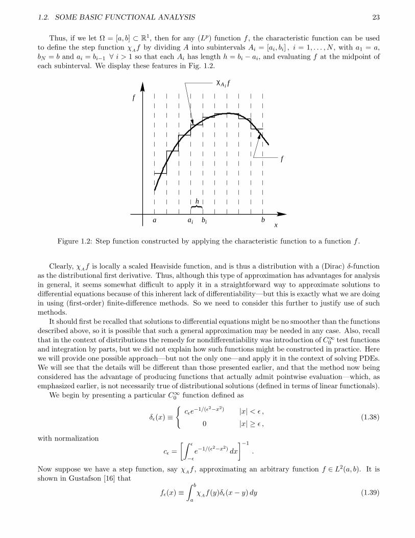
1.2. SOME BASIC FUNCTIONAL ANALYSIS 23
Thus, if we let Ω = [a, b] ⊂ R1, then for any (Lp) function f , the characteristic function can be usedto define the step function χ
Af by dividing A into subintervals Ai = [ai, bi] , i = 1, . . . ,N , with a1 = a,
bN = b and ai = bi−1 ∀ i > 1 so that each Ai has length h = bi − ai, and evaluating f at the midpoint ofeach subinterval. We display these features in Fig. 1.2.
bi
A iχ f
ai b
f
a
h
x
f
Figure 1.2: Step function constructed by applying the characteristic function to a function f .
Clearly, χAf is locally a scaled Heaviside function, and is thus a distribution with a (Dirac) δ-function
as the distributional first derivative. Thus, although this type of approximation has advantages for analysisin general, it seems somewhat difficult to apply it in a straightforward way to approximate solutions todifferential equations because of this inherent lack of differentiability—but this is exactly what we are doingin using (first-order) finite-difference methods. So we need to consider this further to justify use of suchmethods.
It should first be recalled that solutions to differential equations might be no smoother than the functionsdescribed above, so it is possible that such a general approximation may be needed in any case. Also, recallthat in the context of distributions the remedy for nondifferentiability was introduction of C∞
0 test functionsand integration by parts, but we did not explain how such functions might be constructed in practice. Herewe will provide one possible approach—but not the only one—and apply it in the context of solving PDEs.We will see that the details will be different than those presented earlier, and that the method now beingconsidered has the advantage of producing functions that actually admit pointwise evaluation—which, asemphasized earlier, is not necessarily true of distributional solutions (defined in terms of linear functionals).
We begin by presenting a particular C∞0 function defined as
δǫ(x) ≡cǫe
−1/(ǫ2−x2) |x| < ǫ ,
0 |x| ≥ ǫ ,(1.38)
with normalization
cǫ =
[∫ ǫ
−ǫe−1/(ǫ2−x2) dx
]−1
.
Now suppose we have a step function, say χAf , approximating an arbitrary function f ∈ L2(a, b). It is
shown in Gustafson [16] that
fǫ(x) ≡∫ b
aχ
Af(y)δǫ(x− y) dy (1.39)
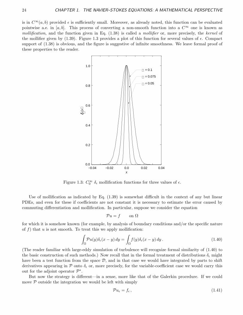
24 CHAPTER 1. THE NAVIER–STOKES EQUATIONS: A MATHEMATICAL PERSPECTIVE
is in C∞(a, b) provided ǫ is sufficiently small. Moreover, as already noted, this function can be evaluatedpointwise a.e. in [a, b]. This process of converting a non-smooth function into a C∞ one is known asmollification, and the function given in Eq. (1.38) is called a mollifier or, more precisely, the kernel ofthe mollifier given by (1.39). Figure 1.3 provides a plot of this function for several values of ǫ. Compactsupport of (1.38) is obvious, and the figure is suggestive of infinite smoothness. We leave formal proof ofthese properties to the reader.
0
0.2
0.4
0.60.6
0.8
1
-0.04 -0.03 -0.02 -0.01 0 0.01 0.02 0.03 0.040.0−0.04 −0.02 0.02 0.04
δ ∋ (x
)
0.0
0.2
0.4
0.6
0.8
1.0
x
∋
∋
∋
= 0.1
= 0.075
= 0.05
Figure 1.3: C∞0 δǫ mollification functions for three values of ǫ.
Use of mollification as indicated by Eq. (1.39) is somewhat difficult in the context of any but linearPDEs, and even for these if coefficients are not constant it is necessary to estimate the error caused bycommuting differentiation and mollification. In particular, suppose we consider the equation
Pu = f on Ω
for which it is somehow known (for example, by analysis of boundary conditions and/or the specific natureof f) that u is not smooth. To treat this we apply mollification:
∫
ΩPu(y)δǫ(x− y) dy =
∫
Ωf(y)δǫ(x− y) dy . (1.40)
(The reader familiar with large-eddy simulation of turbulence will recognize formal similarity of (1.40) tothe basic construction of such methods.) Now recall that in the formal treatment of distributions δǫ mighthave been a test function from the space D, and in that case we would have integrated by parts to shiftderivatives appearing in P onto δǫ or, more precisely, for the variable-coefficient case we would carry thisout for the adjoint operator P∗.
But now the strategy is different—in a sense, more like that of the Galerkin procedure. If we couldmove P outside the integration we would be left with simply
Puǫ = fǫ , (1.41)
1.2. SOME BASIC FUNCTIONAL ANALYSIS 25
as is clear from (1.40). But since the limits of integration are constants for each fixed ǫ, this is possiblewhenever P is a constant-coefficient (and, in particular, linear) operator. Otherwise, there is an inherentcommutation error. Up to estimating the damage done by such errors we see that in principle we cananalytically treat the mollified equation for a nondifferentiable solution as if it were a C∞ function a.e.From a practical, computational standpoint this corresponds to mollification od f , and probably also of u.
In the case of time-dependent problems such as will often be treated in the sequel, there is an alternativeapproach for utilizing mollification. Recall that in such cases we can, in principle, construct a solutionoperator such as Eq. (1.18), an example of which is provided by Eq. (1.17). (We can always constructdiscrete versions of solution operators numerically.) We have not previously discussed properties of solutionoperators, but a particularly important one for our purposes here is
S(t+ s)u0 = S(t)S(s)u0 = u(t) . (1.42)
This is one of several properties required for a family of operators to constitute a continuous semigroup(of operators). The interested reader is referred to texts on functional analysis such as Aubin [23] andGoldstein [24].
The notation of Eq. (1.42) implies that we can solve initial value problems over extended time intervalsby subdividing these into smaller subintervals and solving a new initial value problem on each, using thefinal value attained on the previous interval as the initial data for the next succeeding one. It is easily seenthat essentially all techniques for numerical integration of differential equations make use of this property,but we emphasize that it is not a trivial notion, as is clear from the cited references. We can formallyexpress the above as
S(t)u0 = S(t+ s)u0 = S(t)S(s)u0 = S(t)u(s) = u(t) ,
where 0 < s < t. It is easily seen that typical discrete solution operators satisfy this property (e.g.,consider the forward-Euler approximation to the heat equation), but it is not trivial to demonstrate thisin the continuous case.
It is clear from this (and more particularly, from extensions to larger numbers of subintervals) that wecan actually apply mollification to the solution, itself, rather than to the PDE as done above, and this inturn permits us to treat even nonlinear problems in a natural way. The overall process then begins withmollification of the initial data (if necessary):
u0,ǫ(x) =
∫ ǫ
−ǫu0(y)δǫ(x− y) dy .
ThenS(s)u0,ǫ ≃ u(s) ,
with approximate equality because u0,ǫ(x) does not exactly equal u0(x) at all points of Ω.Now, even though u0,ǫ ∈ C∞(Ω), it can easily be the case that u(s) = S(s)u0,ǫ 6∈ C∞(Ω). Thus, to
compute u(t) we should first apply mollification to u(s) to obtain
uǫ(x, s) =
∫ ǫ
−ǫu(y, s)δǫ(x− y) dy ,
where we have re-inserted explicit notation for spatial dependence of u for clarity. Then we obtain
S(t)uǫ(s) ≃ u(t) .
We remark that it is often the case, especially for nonlinear problems such as those associated with theN.–S. equations, that existence of solutions can be proven only over finite (and sometimes rather short)time intervals. The preceding suggests a way by means of which time of existence might be extended.But it is important to recognize that this is not accomplished without a price. In particular, error mustaccumulate as the result of repeated mollification, so it is necessary to quantify and control such errors
26 CHAPTER 1. THE NAVIER–STOKES EQUATIONS: A MATHEMATICAL PERSPECTIVE
if the result at the final time is to be an accurate representation of the solution to the original problem.(In an analytical problem this error can be formally removed in the limit ǫ → 0, but in a computationalsetting this is not a useful limit because it recovers the non-smooth solution that was causing problems inthe first place.)
We can now relate the preceding to the ability to approximate non-classical solutions using finite-difference and finite-volume procedures. The first point to note is that, as discussed earlier, discretesolutions by their basic nature are nonclassical, and we have already indicated how these are able toconverge to true classical solutions—at least in cases where these are sufficiently smooth. At this point weneed to reconsider what happens to a discrete solution approximating a non-classical one as discretizationstep sizes are decreased.
Suppose the true solution is sufficiently badly behaved that the formal dominant truncation error(obtained via Taylor expansion) is already a δ-function. Then as grid spacing is decreased by increasingthe number of grid points, the number of points at which δ-function like errors occur will also increase,making convergence in a (uniform) pointwise sense impossible (as it must be for weak solutions, and oftenwill be for strong ones at some points). Moreover, in the case of nonlinear problems such errors can easilybe amplified, leading to numerical instability. So it might seem that attempts to accurately approximatenon-classical solutions using difference approximations are doomed to failure. But just as was the case inthe analytical treatment described above, the remedy is mollification. This has been used in many differentforms beginning as early as the 1940s, and in a sense all are equivalent. Here, we emphasize a version ofthis that closely mimics the analytical procedure presented above.
For readers familiar with signal processing, or with any situation in which filters are employed (forexample, large-eddy simulation, LES, of turbulent fluid flow mentioned earlier), it is readily apparent thatEq. (1.39) represents application of a filter with kernel δǫ to the non-smooth function χ
Af . This implies
that if we can find a digital filter to apply to the numerical solution obtained after each step of a discretesolution operator, then we can produce a smooth solution that can, in principle, be made arbitrarily closeto the exact non-classical solution. Figure 1.3 provides a hint as to the nature of a filter applicable tonumerical mollification. In particular, it is apparent from the figure, that independent of the value ofǫ > 0, the graph of δǫ is fairly close to being triangular (but smooth); i.e., it consists, to a fairly goodapproximation, of two straight line segments. In turn, this implies that the product of δǫ and any stepfunction can be integrated exactly via trapezoidal integration provided ǫ is sufficiently small that δǫ spansonly three function values of the (numerical) step function.
It turns out, as we will show in some detail in Chap. 2, that this heuristic argument can be mademore precise to derive a specific form of filter introduced by Shuman [25] for the analysis of atmosphericdata. For now we simply note that such procedures, as well as other similar approaches, are available forconverting non-smooth numerical solutions to smooth ones. We will later provide details of some of these,and furthermore explain exactly how they accomplish the desired end. But we will do this more specificallyin the context of the Navier–Stokes equations. In any case, at this point we expect that we can actuallyproduce numerical approximations to non-classical solutions of PDEs in general, so it is now time to beginstudy of the nature of solutions to the N.–S. equations, which as we will see, are often nonclassical.
1.3 Existence, Uniqueness and Regularity of N.–S. Solutions
In this section we begin by introducing three physically-based ideas somewhat specific to the incompress-ible Navier–Stokes equations and use these to define function spaces needed to precisely state theoremsassociated with existence, uniqueness and regularity of N.–S. solutions. In particular, we will define spacesof functions based on finite energy and enstrophy, along with satisfaction of the divergence-free constraint.We will also present some specific mathematical techniques applied to the N.–S. equations that will bevaluable both in discussing the theorems alluded to above and in understanding the foundations of someof the solution algorithms to be analyzed in the sequel. These will include Helmholtz–Leray projection,construction of weak and Galerkin forms of the N.–S. equations and energy (in)equalities. We conclude
1.3. EXISTENCE, UNIQUENESS AND REGULARITY OF N.–S. SOLUTIONS 27
the section by stating and discussing some of the main well-known results from the mathematical theoryof the Navier–Stokes equations.
1.3.1 Function spaces incorporating physics of incompressible flow
We begin this treatment by reminding the reader of the relationship between functions in L2 and finitekinetic energy, and we describe a corresponding notion associated with the Sobolev space H1 and a physicalquantity known as enstrophy.
Finite Energy and the Function Space H(Ω)
Recall from Eq. (1.8) that a function f is in L2(Ω) if (and only if)
∫
Ω|f |2 dx <∞
where |·| denotes the modulus of f in the sense of complex numbers (and thus can be dropped for real-valuedscalar functions). We can readily extend this to vector-valued real functions, say u = (u(x), v(x), w(x))T
with x = (x, y, z), for example, by replacing the complex modulus with Euclidean length (and retainingthe same notation). Thus, for Ω ⊆ R3 we write
∫
Ω|u|2 dx ≡
∫
Ωu2 + v2 + w2 dxdydz =
∫
Ωu · u dxdydz , (1.43)
which up to a factor of 12ρ, with ρ being fluid density, is the kinetic energy per unit volume. For incom-
pressible flow, ρ ≡ const., and in mathematics it is common to set this constant to unity. Hence, we definethe (mathematical) energy of the flow field in a domain Ω as
e(u) ≡ 1
2
∫
Ω|u|2 dx . (1.44)
Clearly, since e = 12‖u‖2
L2, if u ∈ L2(Ω) the flow has finite energy.
Now recall that the incompressible N.–S. equations comprise a system of initial boundary value problems(whose solutions must be divergence free—recall Eqs. (1.1) and so must have initial and boundary dataprescribed to constitute a well-posed problem. From the perspective of mathematics, it is convenient toinclude at least the boundary data and the divergence-free requirement in definitions of function spaces inwhich solutions might be sought. We thus define the space of functions denoted H on a domain Ω as
H(Ω) ≡f ∈ L2(Ω); ∇·f = 0 , B∂Ωf prescribed
, (1.45)
where B∂Ω denotes the boundary operators on ∂Ω appearing in the boundary conditions of the given N.–S.problem. In words, we say a function f is in the space H(Ω) if it is divergence free, satisfies the prescribedboundary conditions of the problem and has finite energy in Ω in the sense of Eq. (1.44). This functionspace plays a key role in the theory of N.–S. solutions, as will become apparent. We also remark that forvector-valued functions (herein denoted by bold type) containing d components, as we are now treating,the corresponding function spaces are sometimes denoted as, e.g., L2(Ω)d or H(Ω)d. We will not, however,follow this practice in these lectures as it is superfluous if the number of components of f is known. Wefurther note that H(Ω) is not the same as the Sobolev space H1(Ω).

28 CHAPTER 1. THE NAVIER–STOKES EQUATIONS: A MATHEMATICAL PERSPECTIVE
Finite Enstrophy and the Function Space V (Ω)
The term “enstrophy” seldom arises in elementary fluid dynamics—and probably almost never in math-ematics; but it occurs frequently in studies of turbulence because, at least in classical analyses, muchemphasis is placed on the role of vorticity in turbulence generation, and as shown below, enstrophy isessentially the L2 norm of vorticity.
We first recall from elementary fluid dynamics that vorticity is defined as the curl of the velocity vector:
ω ≡ ∇×u .
This is, of course, a vector if u ∈ R3 (but only a scalar for u ∈ R2); so we can write ω = (ω1, ω2, ω3)T and
calculate a quantity analogous to energy (but without the factor of 1/2):
E(u) ≡∫
Ω|ω|2 dx . (1.46)
This equation defines physical enstrophy; clearly, enstrophy is simply the square of the L2 norm of thevector vorticity.
The mathematical definition is slightly different, but equivalent in a sense we will indicate below.Recall that the components of vorticity are computed as differences of velocity derivatives (i.e., fluid parcelangular rotation rates); for example,
ω3 =
(∂v
∂x− ∂u
∂y
).
In light of (1.46) this suggests that enstrophy is associated with (first) derivatives of the velocity field beingin L2(Ω), and hence with the Sobolev space H1(Ω). In turn, this implies we instead might consider the L2
norm of the velocity gradient matrix (tensor):
∫
Ω|∇u|2 dx ,
where now | · | denotes the finite-dimensional matrix 2-norm.Now observe that if we add and subtract the transpose of ∇u, we obtain
∇u =
ux uy uz
vx vy vz
wx wy wz
=1
2
2ux uy + vx uz + wx
vx + uy 2vy vz + wy
wx + uz wy + vy 2wz
+
0 uy − vx uz −wx
vx − uy 0 vz − wy
wx − uz wy − vz 0
.
The first matrix on the right-hand side is the strain rate (tensor), while the second contains the componentsof the vorticity and is sometimes referred to as the rotation tensor. We leave as an exercise to the readerdemonstration that √
2
2|ω| ≤ |∇u| ,
and hence that using
E(u) =
∫
Ω|∇u|2 dx (1.47)
is equivalent to using the physical definition of enstrophy in the sense that if E(u) is finite by Eq. (1.47)then it will also be when calculated in terms of Eq. (1.46), but in general could be either somewhat smalleror larger. Equation (1.47) is the mathematical definition of enstrophy.
1.3. EXISTENCE, UNIQUENESS AND REGULARITY OF N.–S. SOLUTIONS 29
We can write this as
E(u) =d∑
i,j=1
∫
Ω
(∂ui
∂xj(x)
)2
dx ,
where d = 2, 3, and we assume all partial derivatives take on only real values. This leads us to a definitionof the function space usually denoted as V :
V (Ω) ≡f ∈ L2(Ω); ∇·f = 0 , B∂Ωf prescribed , ∇f ∈ L2(Ω)
. (1.48)
In words, the function space V (Ω) consists of those vector-valued functions on Ω that are divergence free,satisfy boundary conditions for the given N.–S. problem and have finite enstrophy. It is clear that onecould replace the finite enstrophy requirement by f ∈ H1(Ω). If we recall Eq. (1.11) and extend this in anatural way to the vector-valued functions we are now considering, we see that the H1 norm of u will begreater than or equal to the square root of the enstrophy.
1.3.2 The Helmholtz–Leray decomposition and Leray projection
In this subsection we will present two pieces of mathematics that are crucial to modern analysis of the N.–S.equations. These are the Helmholtz–Leray decomposition of vector fields and the related Leray projector.It will be evident in Chap. 3 that the latter of these is widely used in modern numerical algorithms employedto solve the incompressible N.–S. equations.
Helmholtz–Leray Decomposition
The Helmholtz decomposition is fairly well known and widely used in specific situations in CFD, forexample in simulation of geophysical flows by spectral methods. It is a special case of a more generalmathematical result known as the Hodge decomposition [26] which can be loosely paraphrased as: any L2
vector field can be decomposed as the sum of curl-free and divergence-free parts. The Helmholtz version ofthis actually applies to functions generally smoother than those simply in L2 (but we could, in principle,use weak forms of the derivatives to circumvent this technicality). It should be further noted that suchdecompositions are not unique, and they do not explicitly account for boundary conditions associated withspecific problems whose solutions might be the vector fields in question.
Leray provided a modification of the above description that addresses both of these two difficulties,and we present this here. We remark that this material is taken nearly verbatim from the monograph byFoias et al. [15].
In constructing a Helmholtz–Leray decomposition we consider a specified vector field v on a boundeddomain Ω ⊂ Rd, d = 2, 3, taking on specified conditions on ∂Ω. We seek a representation of v in the form
v = ∇φ+ u , with ∇ · u = 0 . (1.49)
We will consider any required differentiation in the classical sense, but note that formal (as opposed torigorous) extension to weak derivatives, if necessary, is straightforward, e.g., via mollification. Now observethat in this context ∇φ is clearly curl free (proof of this, using only elementary vector calculus, is left asan exercise for the reader), and u is divergence free by stipulation (but we will see below that this followsfrom the construction used to produce it). The question is whether for a given arbitrary vector field v onΩ we can actually find a scalar φ and a divergence-free vector field u such that the first of Eqs. (1.49) issatisfied.
Application of the divergence operator to (1.49) leaves
∆φ = ∇ · v , (1.50)
which is just a Poisson equation for φ and can be directly solved if boundary conditions for φ in terms ofv can be obtained. If v satisfies no-slip and no-flux conditions, it follows that if we only require u · n = 0
30 CHAPTER 1. THE NAVIER–STOKES EQUATIONS: A MATHEMATICAL PERSPECTIVE
on ∂Ω, we can derive an appropriate boundary condition. In particular, if we take the dot product of thefirst equation in (1.49) with the outward unit normal vector n to ∂Ω, and use the condition just given foru, we see that
∇φ · n = v · n ,or, equivalently, in more suggestive notation,
∂φ
∂n= v · n on ∂Ω . (1.51)
Together, Eqs. (1.50) and (1.51) constitute a Neumann problem for the Poisson equation for φ. To guaranteeexistence of a solution to such problems it is required that the right-hand side of the boundary conditionsatisfy a consistency or compatibility condition of the form (see Stakgold, Vol. II [17] or Garabedian [27])
∫
∂Ωv · n dA = 0 ,
which holds automatically when no-slip/no-flux conditions are imposed on v∣∣∂Ω
. Thus in this case (cor-responding, physically, to solid impenetrable boundaries), we are guaranteed that φ is well defined andunique (only) to within an additive constant. Then u can be computed directly from Eq. (1.49) rearrangedas
u = v −∇φ . (1.52)
Furthermore, applying the divergence operator to both sides of this result, and using Eq. (1.50), showsthat u is indeed divergence free, as required.
We comment that we will encounter an identical construction associated with a particular class ofN.–S. solution algorithms (the projection methods) in Chap. 3 of these lectures, and that the formalismjust presented provides a rigorous justification for use of these methods. We should also note that similarresults can be obtained for periodic boundary conditions for u (see [15]). We leave proof of uniqueness (upto an additive constant) as an exercise for the mathematically-inclined reader. It requires only the mostbasic standard techniques used to prove uniqueness for PDE solutions.
The Leray Projector
Assuming the preceding operations have been carried out, we see that the mapping v 7−→ u(v) on Ωis well defined, and we denote this as
PL : v 7−→ u(v) . (1.53)
This is formal symbolism for the Leray projector. Indeed, PL is a projector, for if v is already divergencefree it will remain unchanged upon application of Eq. (1.52), as follows from the fact that Eq. (1.50)becomes ∆φ = 0 which implies φ ≡ const for the boundary conditions considered here. Hence, P 2
L = PL,as required.
1.3.3 Derivation of “mathematical” forms of the Navier–Stokes equations
There are three forms of the N.–S. equations that have been widely studied by mathematicians, andindeed, the formal theorems to be presented below have been proven within the context of one or more ofthese forms—and not in the form of Eqs. (1.1). This fact tends to lead engineers to conclude that “themathematicians don’t know what they are doing.” But we will show here that the mathematical forms areequivalent to Eqs. (1.1), and in some cases are (almost) directly used in modern simulation procedures.There are three such forms that we will discuss in these lectures: i) an evolution equation (dynamicalsystem) for the velocity field obtained by Leray projection, ii) a weak form of the N.–S. equations andiii) the Galerkin form of the N.–S. equations (which is also a dynamical system, but now expressing timeevolution of the Fourier coefficients—hence, also formally a weak representation).
1.3. EXISTENCE, UNIQUENESS AND REGULARITY OF N.–S. SOLUTIONS 31
For convenience we begin by recalling Eqs. (1.1) and expressing them in a slightly different and moreuseful form:
∂u
∂t+ u · ∇u = −∇p+ ν∆u + F
B(1.54a)
∇ · u = 0 , (1.54b)
where we have divided by the constant density to arrive at kinematic viscosity ν as the coefficient of theLaplace operator; we have also absorbed the density into the pressure (resulting in what is sometimesreferred to as “kinematic” pressure) and the body-force terms without changing their notation from thatof Eqs. (1.1).
Leray Projection of the N.–S. Equations
The reader will recall that earlier (when the solution operator was introduced) we noted it is sometimesconvenient to view the N.–S. equations as a dynamical system. Here we will provide the details of derivingthis particular form. As already hinted, this can be done by Leray projection; the treatment presentedhere follows very closely that found in [15].
From Eq. (1.54b) we see that u must be divergence free (without concern for how this might actuallyoccur—but we know it can be made divergence free via Leray projection). So application of the Lerayprojector, given symbolically in (1.53) and “computationally” in (1.52), results in
PLu = u , PL∂u
∂t=∂u
∂t, and PL∇p = 0 .
Since u is divergence free, validity of the first two of these is obvious. We leave verification of the lastresult to the reader as an exercise in applying Leray projection.
There are three terms remaining in (1.54a) yet requiring projection. The simplest is the body force,and since we have not provided a specific form for this explicitly in terms of physical dependent variables,we will simply represent it symbolically as f = PLF
B. (We note, however, that this is often required to be
divergence free in mathematical analysis of the N.–S. equations.)The next term we consider is the Laplacian of the velocity field, for which the following notation is
standard in mathematical treatments:Au = −PL∆u .
The operator A ≡ −PL∆ is called the Stokes operator. It is worth noting that for periodic boundaryconditions A = −∆ holds, but the case of no-slip conditions is more complicated. In any case, it can beshown that the eigenfunctions of the Stokes operator provide a complete orthonormal basis for constructingFourier representations of N.–S. solutions in the sense described earlier for Sturm–Liouville problems ingeneral (but only in one space dimension). We emphasize that this is not a trivial result due to thenonlinearity of the N.–S. equations. Leray projection of these nonlinear terms is typically representedusing the notation
B(u) = B(u,u) ≡ PL(u · ∇u) .
We now substitute these notations back into Eq. (1.54a) to obtain
du
dt+ νAu +B(u) = f , (1.55)
where we have replaced ∂/∂t with d/dt to emphasize the view that spatial dependence is completelyabsorbed in the operators A, B and in f , and that u = u(t) represents temporal evolution of the vectorfield u(x, t). This suggests the usual notation employed for dynamical systems:
u′ = F (u, t) ,
32 CHAPTER 1. THE NAVIER–STOKES EQUATIONS: A MATHEMATICAL PERSPECTIVE
or if FB
is independent of time,
u′ = F (u) ,
with
F (u) ≡ f − νAu −B(u) .
We note that F (u) contains no explicit information from the pressure. We will see from the Galerkin formof the N.–S. equations, below, how effects of pressure can be incorporated without explicitly includingpressure-gradient terms, and we will later see that not having to explicitly deal with these is a significantadvantage in practical N.–S. solution algorithms.
Weak Form of the N.–S. Equations
We begin by recalling that, in general, the weak form of a PDE is obtained by integrating the PDEagainst C∞
0 test functions ϕ over the domain Ω. That is, we form the scalar product of terms in thePDE with test functions, and then integrate by parts to move derivatives from the nondifferentiable PDEsolution variable to the test function, as in Eqs. (1.28), (1.29) and (1.32). The approach for the N.–S.equations is the same, in principle, but there are differences in details that will be evident as we proceed.
The first difference occurs with the choice of test functions. In obtaining the weak form of the N.–S.equations we employ test functions from the space V (Ω). Thus, instead of being infinitely continuouslydifferentiable as are the functions ϕ ∈ D used previously, the functions v ∈ V (Ω) are only in H1(Ω); i.e.,they have only a single derivative in L2. But we will see that this is all that is needed. Also recall thatfunctions v ∈ V must be divergence free, and they must satisfy the same boundary conditions imposedon the N.–S. solutions, themselves, for any specific problem under consideration. With these basic ideasin mind, we now consider each of the terms in Eq. (1.54a) individually. We will carry out details only forthe case of solid-wall boundaries on which are imposed the usual no-slip/no-flux boundary conditions, butmost of what we present can be employed in cases of other standard boundary conditions, at least aftersome modification.
As is usual, the simplest term is the body-force term, and we write this in weak form as
〈FB,v〉 =
∫
ΩF
B· v dx ,
which clearly is in the form of the L2 (vector) inner product. For this to make sense we must require thatF
B∈ L2(Ω) hold. The next simplest term in Eq. (1.54a) is the time derivative. We have
∫
Ω
∂
∂tu(x, t) · v(x) dx =
d
dt
∫
Ωu(x, t) · v(x) dx ,
which emphasizes the fact that the test functions v depend only on the spatial coordinates, and not ontime. We also require Ω, itself, be independent of time. Then correctness of the above equality is obvious,and we express this as
d
dt〈u,v〉 =
∫
Ω
∂u
∂t· v dx .
We next consider the pressure gradient term of Eq. (1.54a). This leads to
〈∇p,v〉 =
∫
Ω∇p · v dV
=
∫
∂Ωpv · n dA−
∫
Ωp∇ · v dV
= 0 .
1.3. EXISTENCE, UNIQUENESS AND REGULARITY OF N.–S. SOLUTIONS 33
To see that this result holds, we first note that v ∈ V implies ∇ · v = 0 by the definition of the functionspace V ; hence, the second term is zero. The first term is clearly zero as well in the case of no-flux boundaryconditions considered here. We note that other boundary conditions are somewhat more difficult to analyze,but for conditions typical for the N.–S. equations the above result holds generally.
Now we treat the viscous (Laplacian) term. We have, by a direct calculation (left to the interestedreader),
〈∆u,v〉 =
d∑
i,j=1
∫
∂Ω
∂ui
∂xjvi dA−
d∑
i,j=1
∫
Ω
∂ui
∂xj
∂vi
∂xjdV , d = 2, 3 .
(The notation being used here is sometimes referred to as “Cartesian tensor” notation, and is widelyused in classical turbulence formalisms. It corresponds to u = (u1, u2, u3) and x = (x1, x2, x3).) Forno-slip/no-flux boundary conditions vi = 0 on ∂Ω, so the first integral on the right-hand side vanishesleaving
〈∆u,v〉 = −d∑
i,j=1
∫
Ω
∂ui
∂xj
∂vi
∂xjdV .
Similarity of the right-hand side of this equation to the H1 inner product, Eq. (1.11), should be noted.Indeed, in (1.11) we need only start the indexing of the first summation at k = 1 to obtain the form givenabove. There are specific notations for this result, although none appear to be very standard. Since bydefinition ∇v ∈ L2(Ω) must hold for v to be in V , we use the notation
〈u,v〉V (Ω)
≡d∑
i,j=1
∫
Ω
∂ui
∂xj
∂vi
∂xjdV . (1.56)
Finally, we note that little can be done with the nonlinear term beyond introducing some notation forit. The scalar product in this case takes the form
〈u · ∇u,v〉 =
d∑
i,j=1
∫
Ωui∂uj
∂xivj dV ,
and we employ the fairly standard short-hand notation
b(u,u,v) ≡ 〈u · ∇u,v〉 . (1.57)
We now combine the various preceding results and express them in a form that emphasizes temporaldependence, since now the spatial dependence will be integrated out in formally calculating the innerproducts. Thus, the weak form of the N.–S. equations can be written as
d
dt〈u(t),v〉 + ν〈u(t),v〉
V (Ω)+ b(u(t),u(t),v) = 〈F
B,v〉 , (1.58)
which holds ∀ v ∈ V (Ω). Once initial data u(0) = u0(x) have been specified, this equation can beintegrated in time to find 〈u(t),v〉. It should be clear that such a result must correspond to u ∈ H1, butu ∈ H2 is required to have even a strong (but not a classical) solution. Furthermore, the “algorithm”by means of which this might actually be carried out is not obvious. In particular, note that there is nostraightforward procedure for computing ∂ui/∂xj knowing only 〈u,v〉. Hence, it is not clear how 〈u,v〉
V (Ω)
and b(u,u,v) might be evaluated. On the other hand, these forms readily lend themselves to mathematicalanalysis.
One of the more practically useful things (from a mathematical standpoint) that can be obtained fromthe weak form of the N.–S. equations is an energy equation that describes the time evolution of (kinetic)energy of a velocity field, and hence whether the L2 norm of the solution remains bounded. Two thingsare required to derive this. First, we choose a very special test function, viz., u itself. Then we need to

34 CHAPTER 1. THE NAVIER–STOKES EQUATIONS: A MATHEMATICAL PERSPECTIVE
show that b(u,u,u) = 0 in order to obtain the desired result. To show this we observe that using Eq.(1.57) with v = u and the equation preceding this results in
b(u,u,u) =d∑
i,j=1
∫
Ωuj∂ui
∂xjui dV
=1
2
d∑
i,j=1
∫
Ωuj
∂
∂xj
(u2
i
)dV
= −1
2
d∑
i,j=1
∫
Ω
∂uj
∂xju2
i dV
= 0 ,
since
∇ · u =∂u1
∂x1+∂u2
∂x2+∂u3
∂x3= 0 ,
and boundary terms arising from integration by parts in going between the second and third steps dropout due to the no-slip/no-flux conditions.
We also have∫
Ω
∂u
∂t· u dV =
1
2
∫
Ω
∂
∂t(U2) dV =
1
2
d
dt
∫
ΩU2 dV
=d
dte(u) ,
where we have used the notation U2 ≡ u · u. We can now identify Eq. (1.56) with (1.47) to arrive at
d
dte(u) = −νE(u) + 〈F
B,u〉 , (1.59)
which shows that the growth (or decay) of energy of the flow field depends on a balance between dissipationdue to viscosity times enstrophy and forcing from body forces (or boundary conditions). We remark thatalthough the boundary conditions considered here arise frequently in physical problems, there are otherpossibilities, and these must be treated somewhat differently.
The Galerkin Procedure Applied to the N.–S. Equations
We have already presented a fairly detailed, general treatment of the Galerkin procedure in our earlierdiscussions of weak solutions. As noted at that time, this provides a weak form admitting pointwiseevaluation and is thus potentially useful for practical computations. Here we apply this specifically to theN.–S. equations which for simplicity we treat in 2-D dimensionless form in the absence of body forces. Wecan express this case as
ut + (u2)x + (uv)y = −px +1
Re∆u , (1.60a)
vt + (uv)x + (v2)y = −py +1
Re∆v , (1.60b)
ux + vy = 0 . (1.60c)
Here subscripts denote partial differentiation, and ∆ is the Laplacian; Re is the Reynolds number: Re =UL/ν with U and L being appropriate velocity and length scales, respectively. We observe that Eqs.

1.3. EXISTENCE, UNIQUENESS AND REGULARITY OF N.–S. SOLUTIONS 35
(1.60a) and (1.60b) are in so-called “conservation form,” which we will discuss in more detail in Chap.2. Here, we simply note that it is a convenient form of the equations for application of the Galerkinprocedure. Moreover, we note that considerations of 3-D domains and/or including forcing terms does notchange what we shall present in any essential way from the standpoint of the computational process, perse. On the other hand, as will be clear in the next subsection, these impose a significant change in whatis guaranteed regarding nature of solutions.
In Examples 1.2 and 1.3 we earlier expressed the dependent variables in Fourier series; we follow thesame approach here:
u(x, y, t) =
∞∑
k
ak(t)ϕk(x, y) , (1.61a)
v(x, y, t) =
∞∑
k
bk(t)ϕk(x, y) , (1.61b)
p(x, y, t) =
∞∑
k
ck(t)ϕk(x, y) . (1.61c)
As was true in earlier discussions of the Galerkin procedure, k ≡ (k1, k2), and the lower bound for compo-nents of this wavevector is typically one of −∞, 0 or 1. Also, an analogous expansion would be given forthe body force if one were present.
For convenience we will assume Ω is a rectangle and that the boundary conditions used with Eqs.(1.60) are periodicity conditions. Although this is a quite restrictive situation, our main goal here is tointroduce some mathematical notions associated with the N.–S. equations when viewed in Fourier space,so the overall simplicity of this arrangement is an advantage. It is important to note, however, that itis difficult to lift these conditions and retain a numerically efficient procedure; as a consequence, mostcomputer implementations of this method are quite similar to the version we will discuss here.
In light of the periodicity conditions we can employ complex exponentials as basis functions; that is,we set
ϕk(x, y) = eik·x = ei(k1x+k2y) = eik1xeik2y . (1.62)
The last form on the right is often termed a “tensor product” basis because its two factors are defined inan uncoupled way on two separate copies of subsets of R1.
To begin construction of the Galerkin form of Eqs. (1.60) we start with the simplest, Eq. (1.60c), thedivergence-free condition, or continuity equation. We substitute Eqs. (1.61a) and (1.61b) into this equationand commute summation and differentiation to obtain
i∞∑
k
(k1ak + k2bk)ϕk = 0 .
Since this must hold at all points of Ω (or, at least a.e. in Ω), and ϕk 6≡ 0, we must have
k1ak + k2bk = 0 ∀ k . (1.63)
Similarly, if we substitute these expansions into the x-momentum equation (1.60a), we obtain
∂
∂t
∑
ℓ
aℓϕℓ +∂
∂x
∑
ℓ,m
aℓamϕℓϕm +∂
∂y
∑
ℓ,m
aℓbmϕℓϕm =
− ∂
∂x
∑
ℓ
cℓϕℓ +1
Re
[∂2
∂x2
∑
ℓ
aℓϕℓ +∂2
∂y2
∑
ℓ
aℓϕℓ
].

36 CHAPTER 1. THE NAVIER–STOKES EQUATIONS: A MATHEMATICAL PERSPECTIVE
Again commuting summation and differentiation yields
∑
ℓ
aℓϕℓ + i∑
ℓ,m
(ℓ1 +m1)aℓamϕℓϕm + i∑
ℓ,m
(ℓ2 +m2)aℓbmϕℓϕm= −i∑
ℓ
ℓ1cℓϕℓ −1
Re
∑
ℓ
(ℓ21 + ℓ22
)aℓϕℓ .
It can be seen that solutions (the aℓs, bℓs, cℓs) to this equation can be complex, but we are only interestedin those that are real if we are considering solutions corresponding to physical fluid flow. Indeed, if we hadused sine and cosine as basis functions rather than the otherwise more convenient complex exponentials,this would not have been a concern. Furthermore, the reader will recall that sines and cosines may beexpressed in terms of complex exponentials in any case (and conversely). This suggests that a meansof avoiding the potentially complex solutions should be available. In fact, all that is required is settinga−k = ak, where the overbar denotes complex conjugate, and the imaginary parts become zero (see, e.g.,[15]).
This permits us to consider the preceding equation without the imaginary factors i and proceed for-mally. (This is not exactly what is actually done in a computational setting, but it is sufficient for ouranalytical purposes.) We now form inner products of each basis function with the above equation and useorthonormality of ϕk to obtain
ak +∑
ℓ,m
A(1)kℓm
aℓam +∑
ℓ,m
B(1)kℓm
aℓbm = −k1ck − |k|2Re
ak , ∀ k . (1.64)
In these equations the A(1)kℓm
s and B(1)kℓm
s, sometimes termed Galerkin triple products, are defined as, forexample,
A(1)kℓm
≡ (ℓ1 +m1)
∫
Ωϕkϕℓϕm dV , (1.65)
where the superscript (1) denotes the x-momentum equation. Clearly, an analogous result holds for they-momentum equation:
bk +∑
ℓ,m
A(2)kℓm
bℓam +∑
ℓ,m
B(2)kℓm
bℓbm = −k2ck − |k|2Re
bk . (1.66)
At this point we should recall that in both of the two forms of the N.–S. equations considered previously(Leray projected and weak) it was possible to eliminate pressure from the momentum equations, suggestingthat this should be possible also in the present case. If we view Eqs. (1.64) and (1.66) as a vector equationfor the vector (ak, bk) of Fourier coefficients, we can take the dot product of these equations with thewavevector k = (k1, k2) to obtain
k1ak + k2bk +∑
ℓ,m
[k1
(A
(1)kℓm
aℓam +B(1)kℓm
aℓbm
)+ k2
(A
(2)kℓm
bℓam +B(2)kℓm
bℓbm
)]
= −(k21 + k2
2
)ck − |k|2
Re(k1ak + k2bk) ∀ k .
From Eq. (1.63) we see that the first term on the left-hand side and the second on the right-hand sideare both zero, and moreover, we can solve what remains for ck in terms of only the aks and bks:
ck = − 1
|k|2∑
ℓ,m
[k1
(A
(1)kℓm
aℓam +B(1)kℓm
aℓbm
)+ k2
(A
(2)kℓm
bℓam +B(2)kℓm
bℓbm
)]. (1.67)
This implies, as we expected, that Eqs. (1.64) and (1.66) can be expressed in a form that is independent ofpressure, just as was true in the previous cases. But beyond this it explicitly demonstrates the quantitative
1.3. EXISTENCE, UNIQUENESS AND REGULARITY OF N.–S. SOLUTIONS 37
dependence of pressure on nonlinear aspects of the velocity field—in Fourier space. Furthermore, Eq. (1.67)can be substituted into these equations without altering their form.
Independent of this, it is worthwhile to examine some of the details of the Galerkin form of the N.–S.equations. We first make the obvious observation that this form comprises a system of equations for thetime evolution of the Fourier coefficients of the velocity components, and as such is a dynamical system.Furthermore, at each instant in time for which ak(t) and bk(t) are known the Fourier coefficients for pressurecan be calculated directly from Eq. (1.67), and these coefficients can be inserted into Eqs. (1.61) to obtainvalues of u, v and p at any point x ∈ Ω. Of course, in practice these Fourier representations can containonly a finite number N of terms, so the results are only approximate. But at least for solutions possessinga high degree of regularity, the Fourier representations converge very rapidly (in fact, exponentially fast),so not many terms are needed to obtain accurate approximations. For the reader interested in this feature,as well as numerous other details associated with these types of approximations, the monograph by Canutoet al. [28] is recommended.
It is also of interest to note that a Galerkin procedure might be applied to the Leray-projected formof the N.–S. equations given in Eq. (1.55). The natural basis set for this is the set of eigenfunctions of theStokes operator, but other bases might be used as long as some provision is made regarding satisfaction ofthe divergence-free constraint.
Our main purpose in presenting the Galerkin form of the N.–S. equations is to demonstrate how thisFourier-space representation can be used to deduce qualitative mathematical (and physical) features ofN.–S. flows. Here, we consider only the x-momentum equation (1.64); but the same treatment applies toy-momentum, and extension to 3-D flows occurs in a natural way. We begin by temporarily neglecting allnonlinear terms in Eq. (1.64). Then what remains is
ak = −|k|2Re
ak , (1.68)
the solution of which is
ak(t) = ak(0)e−|k|2
Ret , (1.69)
where
ak(0) ≡∫
Ωu0(x)e−ik·x dV . (1.70)
Clearly, this solution decays in time and approaches zero as t → ∞. Moreover, the rate at which thisoccurs is |k|2/Re. In particular, for fixed Re higher-wavenumber Fourier modes decay faster than do lowerones. From a mathematical perspective this suggests (but does not prove) convergence of the Fourier seriesrepresentation and, hence, existence of solutions of the form Eqs. (1.61). On the other hand, if |k| is fixed,then the rate of decay of ak decreases with increasing Re. Now if we recall that the right-hand side of Eq.(1.68) is precisely the Fourier-space representation of the viscous terms of Eq. (1.60a), we see that we canassociate the rate of decay of ak with viscous dissipation; in particular, increasing Re implies decreasingviscous dissipation, and conversely.
We now consider effects of the nonlinear terms. To do this we first drop the linear viscous dissipationterm from Eq. (1.64), and we also drop the term containing ck arising from the pressure gradient in Eq.(1.60a) since, as can be seen from Eq. (1.67), this is directly related to the nonlinear terms, so nothing islost at the qualitative level by ignoring it. Then we are left with
ak = −∑
ℓ,m
[A
(1)kℓm
aℓam +B(1)kℓm
aℓbm
]. (1.71)
We first observe that when ℓ = m a quadratic term appears in the equation. It is worthwhile to considerthe effects of this alone since an analytical solution can be obtained, and this will provide at least someinsight into the qualitative behavior of the nonlinear terms in general. Thus, we solve the initial-valueproblem
ak = −A(1)a2k , (1.72)
38 CHAPTER 1. THE NAVIER–STOKES EQUATIONS: A MATHEMATICAL PERSPECTIVE
with ak(0) again given by Eq. (1.70) and subscript notation for A(1)kℓm
suppressed. We leave as a simpleexercise to the reader demonstration that
ak(t) =1
A(1)t+ 1/ak(0).
It is clear from this that if A(1)ak(0) > 0, then |ak| → 0 as t → ∞, although only algebraically. But ifA(1) and ak(0) are of opposite signs, ak(t) → ∞ can occur in finite time. This implies a potential for veryill behavior (including nonexistence after only a finite time) of N.–S. solutions. We will see in the nextsection that more sophisticated analyses of the 2-D case than considered here show this does not actuallyoccur, but in 3D it is still considered a possibility.
There is a further aspect of the behavior of the terms on the right-hand side of Eq. (1.71) that deservesmention. It is that such nonlinearities can generate new Fourier modes not present in the original repre-sentation (or in initial data for the problem). Consideration of this will be important in Chap. 2 when webegin studies of discretization of the N.–S. equations. Here we consider only the first advective term of thex-momentum equation, (u2)x, and recall its Fourier representation:
(u2)x =∂
∂x
N∑
ℓ,m
aℓamϕℓϕm ,
written now for only a finite numberN of Fourier modes, as would be required for computer implementation.Now if the basis set ϕk is similar to complex exponentials or trigonometric functions we see that,
e.g.,ϕℓ(x)ϕm(x) = eiℓ·xeim·x = ei(ℓ+m)·x .
Since each of ℓ and m can be as large as N , their sum can be greater than N , and the corresponding nonlin-ear term aℓam generates solution behaviors that cannot be resolved by the given N -mode representation.We will return to this in Chap. 2. We note here that this does not occur for the Galerkin procedure dueto the values taken on by the Galerkin triple products and the intrinsically global nature of the Galerkinconstruction; but it does occur for the various Fourier collocation methods that are widely used as a moreefficient alternative to the Galerkin procedure (see [28]). Moreover, it is easily argued that this must occurfor finite-difference and finite-volume methods as well.
Finally, we emphasize that the actual time evolution of each of the aks is effected by combinationsof all the abovementioned behaviors, and as a consequence solutions can be very complicated—and verydifficult to simulate. (The reader may wish to combine Eqs. (1.68) and (1.72), find an exact solution, andanalyze its properties.)
1.3.4 The main well-known N.–S. solution results
In this section we will present the key results of this chapter, the main theorems on existence, uniquenessand regularity of solutions to the Navier–Stokes equations. While practitioners of CFD have a generaltendency to pay little attention to such results we emphasize, as we have already in these lectures, thatit is best to heed and, to the greatest extent possible, use the results from pure mathematics. At thesame time it is recognized that these are often difficult to comprehend, and it has been the purpose ofthe foregoing sections to develop the material that should now make at least a superficial understandingpossible.
The theorems we will state and discuss can be classified as pertaining to 2-D or to 3-D flows, andas to whether they relate to weak or strong solutions to the N.–S. equations. With regard to theseclassifications, it is usually said that essentially everything worth proving for 2-D problems has beenproven. In particular, existence and uniqueness of solutions, both weak and strong, have been provenfor all time beyond any specified initial time for quite reasonable (physically) problems. In 3D, long-timeexistence can be demonstrated for weak solutions, but uniqueness has not been proven for this case. On the

1.3. EXISTENCE, UNIQUENESS AND REGULARITY OF N.–S. SOLUTIONS 39
other hand, only short-time existence has been proven for 3-D strong solutions, but it is known that theseare unique. Especially with regard to existence of strong solutions, the constraints that must be imposedon the shape of the domain Ω (in particular, smoothness of ∂Ω), the boundary and initial conditions, andparticularly on body-force terms and Reynolds number (∼viscosity), can be quite stringent if solutions areto be proven to exist for any but very short times.
Thus, the longstanding mathematical problem, first identified by Leray in the early 1930s, is proof ofexistence and uniqueness of strong (but not necessarily classical) solutions to the N.–S. equations for longtimes, and under reasonable physical conditions. It is of interest to mention that this problem is consideredto be one of the most important problems in mathematics for the 21st Century, and it carries a $1 million“price on its head.” Quite literally, the first person who succeeds in rigorously solving this problem willbe awarded a prize of a million dollars!
In earlier subsections we constructed weak forms of the N.–S. equations, and we defined the strong formas studied by mathematicians: in the next two subsections we will provide a few of the important well-known results for solutions to the Navier–Stokes equations, first in 2D and then in 3D in this framework.(This treatment closely follows that of Foias et al. [15], and as noted in that work, the results were alreadyknown to Ladyzhenskaya [4].) Then, in a final subsection we will summarize some basic conclusions thatimpact the choice of numerical algorithms for solving the N.–S. equations, and at the same time providean indication of what we should expect regarding the qualitative nature of solutions.
Solutions to the N.–S. Equations in 2D
As we noted above, the 2-D N.–S. problem is generally viewed as having been completely solved in themathematical sense. Here we present two of the main results that have contributed to this understanding.We begin with the following theorem on existence and uniqueness for weak solutions, i.e., solutionsto Eq.(1.58) which we repeat here for easy reference:
d
dt〈u(t),v〉 + ν〈u(t),v〉
V (Ω)+ b(u(t),u(t),v) = 〈F
B,v〉 .
Theorem 1.1 Let u0, FB
and tf > 0 be given such that
u0(x) ∈ H(Ω) , and FB(x, t) ∈ L2(0, tf ;H) .
Then ∃ a unique solution u = (u1, u2)T of Eq. (1.58) ∋
ui ,∂ui
∂xj∈ L2(Ω×(0, tf )) , i, j = 1, 2 ,
and u is continuous from [0, tf ] into H. Moreover, the following energy equation holds for t ∈ [0, tf ]:
1
2
d
dt‖u(t)‖2
L2+ ν‖u(t)‖2
H1= 〈F
B(t),u(t)〉 .
There are a number of remarks to be made regarding this theorem. First, no restriction has been placedon the value of the final time, tf , other than it be greater than zero—backward in time N.–S. problems areill posed, and tf = 0 would be trivial. Likewise, no restrictions are placed on the domain Ω. Second, fromthe definition of H(Ω) (Eq. (1.45)), it is clear that u0, the initial data, must be divergence free, and that itmust satisfy whatever boundary conditions have been imposed on u. Thus, initial and boundary data arecompatible in the usual sense of elementary PDE theory, modulo the fact that this need only hold a.e. ina neighborhood of ∂Ω. Furthermore, again from the definition of the function space H, we see that bothu0 and F
Bmust be in L2(Ω) with respect to spatial coordinates, and F
Bmust also be in L2 with respect
to the time interval (0, tf ); moreover, FB
must be divergence free. We remark that this last requirementoften cannot be realized in physical problems.

40 CHAPTER 1. THE NAVIER–STOKES EQUATIONS: A MATHEMATICAL PERSPECTIVE
We next observe that the theorem statement conclusions indicate that the solution to the weak form ofthe N.–S. equations (1.58) is unique. Rather generally, weak solutions typically are not unique. Moreover,the fact that both ui and ∂ui/∂xj , i, j = 1, 2 are in L2 for all time implies that the solutions are actuallyin H1(Ω). Thus, we see that the Navier–Stokes equations in this 2-D setting are providing smoothing; thesolution operator is mapping L2 initial data (and forcing function) into a solution in H1. In addition, thefact that u is continuous for [0, tf ] to H means that if only a small change in time is considered, then thechange of the L2 norm of u during this time will be small. Finally, satisfaction of the energy equality showsthat the L2 norm of u is bounded for all time, provided F
B∈ L2, as required in the theorem statement.
We now state an analogous result concerning strong solutions. We remind the reader of Def. 1.6 for astrong solution, viz., a solution possessing sufficient derivatives to permit evaluation of the correspondingdifferential equation a.e. in the domain Ω, leading to an ability to calculate a desired Lp norm of theequation “residual.”
Theorem 1.2 Suppose u0, FB
are given and are such that
u0(x) ∈ V (Ω) , and FB(x, t) ∈ L2(0, tf ;H) ,
for tf > 0. Then ∃ a unique (strong) solution u = (u1, u2)T with
ui ,∂ui
∂t,∂ui
∂xj,∂2ui
∂xj∂xk∈ L2(Ω×(0, tf )) , i, j, k = 1, 2 ,
and u is continuous from [0, tf ] into V .
As was true for the preceding theorem, this result requires considerable explanation for those not wellversed in the mathematics involved. We should first note that the requirement on u0 is stronger in thiscase; in particular, u0 must now be in V rather than in H, implying that it must be once differentiablea.e. and thus in H1(Ω) instead of only in L2. On the other hand, requirements on the forcing function F
B
remain the same as in the previous case.As a result of this change in required smoothness of initial data, the first derivative with respect to
time and the second with respect to space are now in L2, implying that Eqs. (1.60) can be evaluated a.e.in Ω. Hence, the L2 norm of the differential equation exists, and the solution u is strong in the sense ofDef. 1.6. Here, we have relaxed the C1 condition in time of that definition to continuity in time, but westill must require that ∂ui/∂t exist a.e. in Ω for (almost) every t ∈ (0, tf ]. We should also again observethe smoothing properties of the N.–S. operator. Namely, in the present case initial data were in H1, andthe solution evolved so as to be in H2; this should be expected, at least in an heuristic and qualitativeway, due to the viscous dissipation of the diffusion terms of Eqs. (1.60).
There are two other important points to make at this time. The first is that because both weak andstrong solutions can be proven to be unique, it follows that, in fact, there is only one solution—and it isstrong. It is easily checked (and we leave this as an exercise) that strong (and even classical) solutionssatisfy the weak form of the equations, as noted earlier in our initial discussions of strong solutions (but, ofcourse, the converse is not true). Thus, if both weak and strong solutions exist and are unique, the uniquestrong solution must also be the unique weak one. We comment that it is often the practice in PDE theoryto take the path of first proving weak results followed by proving strong results, and then attempting toshow they are the same.
The final remark of this section is emphasis that although we have indicated existence of unique, strongsolutions to the N.–S. equations (1.60), for all time in 2D, this does not imply that such solutions areany more regular than H2 in space and H1 in time. This has important implications concerning thechoice of numerical methods to be used in implementing CFD algorithms (as was recognized already byRichtmyer and Morton [29], but seems to have been ignored in recent years) because it indicates that theTaylor series needed for truncation error analysis may not exist, and in turn, use of high-order methodsis not likely to produce uniformly superior results. But in addition, this suggests that mollification (often
1.3. EXISTENCE, UNIQUENESS AND REGULARITY OF N.–S. SOLUTIONS 41
termed regularization, especially in the numerical analytic context) will probably be needed, especiallywhen coarse discretizations are used, to control growth of effects from unrepresented high modes arisingfrom nonexistence of high-order derivatives and from nonlinear terms. Details of this will be provided inChap. 2.
Solutions to the N.–S. Equations in 3D
The results we present in this subsection are in many respects quite similar to those given above fortwo space dimensions. But there are important differences as we will note in the following discussions. Weagain first provide results associated with weak solutions, and follow this with corresponding results forstrong solutions.
Theorem 1.3 Let u0, FB
and tf > 0 be given and such that
u0(x) ∈ H(Ω) , and FB(x, t) ∈ L2(0, tf ;H) .
Then ∃ at least one solution u = (u1, u2, u3)T to Eq. (1.58) ∋
ui,∂ui
∂xj∈ L2(Ω×(0, tf )) , i, j = 1, 2, 3,
and u is weakly continuous from [0, tf ] into H.
We first remind the reader that weak continuity was introduced in Def. 1.2 in terms of linear functionalsbased on C∞
0 test functions. But here we will replace these test functions with functions v(x) ∈ V (Ω) (⊂H1). Then weak continuity of u implies that ∀ v ∈ V the mapping
t 7−→ 〈u(x, t),v(x)〉 =
∫
Ωu(x, t) · v(x) dV
must be continuous (in the usual sense). We should note that this is different from the 2-D case in whichcontinuity of u into H was strong. A second difference from the 2-D case is that weak solutions in 3D maynot be unique (it is currently not known whether they are, or not). Finally, in place of the energy equalitygiven in Theorem 1.1, only an energy inequality can be proven for the 3-D case:
1
2
d
dt‖u(t)‖2
L2+ ν‖u(t)‖2
H1≤ 〈F
B(t),u(t)〉 ,
in which all differentiations must be taken in the sense of distributions constructed with L2 and H1 innerproducts, as appropriate for individual terms.
Theorem 1.3 clearly is not a very favorable result; its one good feature is that there is no restriction ontf ; i.e., we have global in time existence, but possibly nonuniqueness, of the weak solution(s) in 3D. Wewill now see that, in a sense, just the opposite holds for strong solutions.
Theorem 1.4 Let u0, FB
and tf > 0 be given and such that
u0(x) ∈ V (Ω) , and FB(x, t) ∈ L2(0, tf ;H) .
Then ∃ t∗∈(0, tf ] and depending on u0, FB, ν and Ω ∋ there is a unique strong solution u = (u1, u2, u3)
T
to Eqs. (1.60) with the properties
ui,∂ui
∂t,∂ui
∂xj,∂2ui
∂xj∂xk∈ L2(Ω×(0, t∗)) , i, j, k = 1, 2, 3 ,
and u is a (strongly) continuous function from [0, t∗) into V .

42 CHAPTER 1. THE NAVIER–STOKES EQUATIONS: A MATHEMATICAL PERSPECTIVE
It is of interest to note that by arguments analogous to those used in 2D, we see that uniquenessof this solution implies that there is no other solution—strong or weak—on the interval [0, t∗). But wecannot prove existence of any strong solution beyond the time t∗, while time of existence for the possiblynonunique weak solution(s) is unlimited.
We should again observe that just as in 2D, we bought better solution behavior by requiring moreregular initial data. But in the present case we can only prove such a solution exists for a finite time, atime which is influenced by essentially everything associated with the problem. Constantin and Foias [13]can be consulted for more details on this aspect of N.–S. solutions; here we simply note that, e.g., as Rebecomes large (and hence dissipation, i.e., ν, becomes small), the provable time of existence of a strongsolution becomes short—as one might expect.
Some Conclusions
We end this section with some basic conclusions that are easily deduced from the foregoing discussions.First, it is clear in both 2D and 3D that the nature of initial data has a significant impact on ultimateregularity of N.–S. solutions. In particular, for the theorems quoted here it is necessary that initial data bedivergence free and be compatible with boundary conditions. Without these restrictions it is not clear thateven existence can be proven; but at the very least, if these requirements are not met, smoothness of N.–S.solutions will be reduced. Thus, the first step in any computational algorithm for solving the incompressibleN.–S. equations should be mollification to achieve boundary compatibility followed by projection of themollified initial data to a divergence-free subspace via Leray projection.
Furthermore, there is no prescription for initial pressure in any of the theorem statements. In the caseof weak solutions pressure does not enter the problem in any direct way, so this is to be expected. But forstrong solutions this could be different, and in either case it leaves open the question of how to handle thisin the context of numerical methods that generally do not employ divergence-free bases. In particular, itshould be clear that regardless of any algorithmic details, pressure (initial, or otherwise) must be obtainedfrom the velocity field (recall the Galerkin representation of the N.–S. equations, for example) so as to beconsistent with the divergence-free condition.
The next thing to note is that the forcing function FB
has also been required to be divergence free; itis a mapping from H to L2. In physical problems, as mentioned earlier, this might not be the case—andthere may be nothing that can be done to improve the situation. Hence, solution behavior may be worsethan indicated by the theorems of this section. On the other hand, with F
B≡ 0, as often occurs, the given
results probably represent a “worst case.” But even so, as we have already noted, especially in the mostimportant case of 3-D flows at high Re, it is unlikely that solutions will be classical. As a consequence,much of Taylor series based numerical analysis is inapplicable without modification. We will treat somedetails of this in the next chapter.
1.4 Summary
In this introductory chapter we have provided some basic notions from functional analysis—definitions ofvarious function spaces, linear functionals and distributions—that permit us to understand the conceptsof weak and strong solutions to partial differential equations. In addition we have presented variousmathematical techniques that are crucial for being able to analyze the N.–S. equations: mollification,Helmholtz–Leray decomposition, Leray projection and the Galerkin procedure. These tools permittedus to discuss weak and strong solutions to PDEs in general and to construct various forms of the N.–S.equations. We then stated and discussed some of the main theorems describing existence, uniqueness andregularity properties of N.–S. solutions. We have emphasized that in three space dimensions the theory ofthese equations is incomplete: existence of weak solutions can be proven for all time, but it is not knownwhether such solutions are unique; existence and uniqueness of strong solutions can be proven only for finitetime. Finally, we have stressed that even strong solutions are considerably different from classical ones, and

1.4. SUMMARY 43
generally do not possess sufficient regularity for typical Taylor series based approaches to error analysis.This casts doubt on, among other things, the utility of attempting to employ higher-order methods whenapproximating solutions to the Navier–Stokes equations, and it implies that considerable care must beexercised in constructing solution algorithms and in attempting to validate computed results.

44 CHAPTER 1. THE NAVIER–STOKES EQUATIONS: A MATHEMATICAL PERSPECTIVE
Chapter 2
Special Numerical Difficulties of the
Navier–Stokes Equations
In this chapter we present several mathematical/numerical analytic topics that are quite specific to treat-ments of the Navier–Stokes equations. We begin by summarizing essentially all the different forms intowhich the N.–S. equations have been cast during attempts to solve them. We follow this with a descriptionof the various grid structures one can consider and compare advantages and disadvantages of these as theyrelate to the problem of pressure-velocity coupling. Finally, we treat the problem associated with cell-Rerestrictions on difference approximations and grid spacing, and we conclude the chapter with discussionspertaining to the related problem of aliasing.
2.1 Forms of the Navier–Stokes Equations
The N.–S. equations have, through the years, been cast in many different forms during attempts to solvethem, especially in 2D. Here we will review essentially all of these. But we note that the main purpose ofthis is to allow the reader to recognize that in the current era of very powerful computing hardware it isseldom that anything but the so-called “primitive-variable” form of the equations is employed. Thus, wewill begin this section with this basic form. We follow this with the stream function/vorticity formulationthat once was widely used for 2-D calculations, and we then consider the velocity/vorticity formulation.Finally, we return to the primitive-variable equations and consider various modifications of these thatsometimes can provide specific advantages.
2.1.1 Primitive-variable formulation
We previously presented the N.–S. equations in Chap. 1 as
ρDu
Dt= −∇p+ µ∆u + F
B, (2.1a)
∇ · u = 0 . (2.1b)
Here, ρ and µ are constant density and viscosity, and FB
is a body force. The dependent variables inthis equation are the velocity vector u = (u, v,w)T and the pressure p. This set of variables is termed“primitive” since in most typical laboratory experiments it includes the physical variables that can bedirectly measured. Moreover, other quantities of interest in a fluid flow (e.g., vorticity or circulation)can be computed directly from these. It is important to recognize, however, that the body force F
Bmay
contain further dependent variables, e.g., temperature T , and when this is the case additional transport(or other) equations will be required. For the present we ignore such added complications beyond notingthat typical body forces arise from buoyancy, rotation and electromagnetic fields.
45
46 CHAPTER 2. SPECIAL NUMERICAL DIFFICULTIES OF THE NAVIER–STOKES EQUATIONS
A fundamental observation associated with Eqs. (2.1) is that the momentum equations (2.1a) should beviewed as the equations that describe the velocity field, while the divergence-free condition (2.1b) providesan equation for pressure. This should seem rather natural in light of our discussions in Chap. 1 where itwas shown that the momentum equations can be solved for the velocity field in the absence of pressuregradient terms. This leaves only ∇ · u = 0 for finding the pressure; indeed, it is often said that “pressureenforces the divergence-free constraint in an incompressible flow.” But this equation does not explicitlycontain the pressure, and this has caused significant problems from a computational standpoint; we willconsider several treatments of these difficulties in the sequel.
The first attempts to rectify this problem arose from recognition that a Poisson equation for pressure(the so-called PPE) can be derived by calculating the divergence of Eq. (2.1a): we have
ρ∇ · Du
Dt= −∇ · (∇p) + µ∇ · ∆u + ∇·F
B,
or after commuting the divergence operator with other differential operators wherever this is convenient(and appropriate) we have (after expanding the substantial derivative)
ρ∂(∇ · u)
∂t+ ρ∇ · (u · ∇u) = −∆p+ µ∆(∇ · u) + ∇·F
B,
or
∆p = ∇·FB
+ µ∆(∇ · u) − ρ
[∂(∇ · u)
∂t+ ∇ · (u · ∇u)
]. (2.2)
This implies that pressure can be calculated provided the velocity field is known, a result we earlier deducedfrom the Galerkin form of the N.–S. equations. But Eq. (2.2) requires boundary conditions at all points onthe boundary of the solution domain Ω. This fact led to considerable misunderstandings regarding solutionof the N.–S. equations (see, e.g., Gresho and Sani [30]) and was one of the motivations for solving variousalternative forms of the equations of motion we will discuss in subsequent sections.
Before turning to these, however, there are two main points that should be made regarding Eq. (2.2).The first is that if we assume that (2.1b) is satisfied, Eq. (2.2) collapses to
∆p = ∇·FB− ρ∇ · (u · ∇u) . (2.3)
Moreover, if FB∈ H(Ω), as required by hypotheses of the theorems concerning existence, uniqueness and
regularity of N.–S. equation solutions given in Chap. 1, this becomes
∆p = −ρ∇ · (u · ∇u) .
Thus, if we have somehow obtained a divergence-free velocity field we can determine the pressure fromthis equation supplemented with appropriate boundary conditions, which we will treat in more detail in alater section. But we note here that on solid surfaces the pressure usually is not known and is typically amajor part of the desired information to be obtained by solving the problem.
The second thing to observe regarding use of (2.2) or (2.3) is that it does not accomplish the desiredtask of forcing the velocity field to be divergence free. In fact, within the confines of the description givenhere it is necessary to already have a divergence-free velocity in order to use Eq. (2.3) (or the equationfollowing it). Moreover, solutions to the momentum equations (2.1a) are not necessarily divergence free(and this is all the more true of their discrete representations). Clearly, if they were, the constraint (2.1b)would be unnecessary. But we have already seen in Chap. 1 a procedure for obtaining a divergence-freevelocity field—Leray projection, and we will later see that this provides a crucial computational tool inthe present context.
2.1. FORMS OF THE NAVIER–STOKES EQUATIONS 47
2.1.2 Stream function/vorticity formulations
Difficulties with satisfying the divergence-free condition and prescribing boundary conditions for pressureled researchers to seek formulations that did not include the pressure, and which automatically enforcedthe divergence-free constraint. The first, and probably the most successful, of these is the stream func-tion/vorticity formulation. The stream function was widely used in analytical treatments of the N.–S.equations (e.g., in boundary-layer theory), so this was a natural approach. But it possesses two majorshortcomings, the first of which is that there is no straightforward extension of the 2-D formulation to 3D.
We begin this section with the basic, well-known 2-D treatment, and follow this with a brief discussionof a possible way to handle 3-D cases.
2-D Stream Function/Vorticity
Consider a velocity field u = (u, v)T defined on a domain Ω and the divergence-free constraint
ux + vy = 0 . (2.4)
We wish to find a way to automatically satisfy this condition. It is clear for any function ψ ∈ C2(Ω) thatits mixed partial derivatives satisfy
ψxy = ψyx .
It follows that we should define the stream function ψ by
u = ψy , and v = −ψx . (2.5)
Then Eq. (2.4) is automatically satisfied. Thus, if we could find a PDE satisfied by ψ, and related toproperties of the flow field, we would be able to obtain a divergence-free velocity field via Eqs. (2.5).
To do this we first recall that in 2D the vorticity vector has only a single component,
ω = vx − uy . (2.6)
Now substitution of Eqs. (2.5) into this yields
∆ψ = −ω , (2.7)
so if we can find an equation for ω we will have obtained a formulation that automatically producesdivergence-free velocity fields. While the formal equivalence of this formulation with the N.–S. equationsrequires rigorous proof, the construction we will employ is suggestive, and we will not be further concernedwith this approach in any case.
In 3D we would take the curl of the momentum equations to produce the desired result. But in 2D itis easier to simply “cross differentiate” the two momentum equations, and then subtract the x-momentumequation from the y-momentum equation. In this case the equations are (in the absence of body forces)
ρ (ut + uux + vuy) = −px + µ∆u , (2.8a)
ρ (vt + uvx + vvy) = −py + µ∆v , (2.8b)
and cross differentiation leads to
ρ (uyt + uyux + uuxy + vyuy + vuyy) = −pxy + µ∆uy ,
ρ (vxt + uxvx + uvxx + vxvy + vvxy) = −pxy + µ∆vx ,
where we have assumed sufficient smoothness to permit changing the order of differentiation whenever thisis convenient.
48 CHAPTER 2. SPECIAL NUMERICAL DIFFICULTIES OF THE NAVIER–STOKES EQUATIONS
Next substract the first of these from the second to obtain
ρ(vx − uy)t + (vx − uy)ux + (vxx − uxy)u+ (vx − uy)vy + (vxy − uyy)v = µ∆(vx − uy) .
We observe that the second and fourth terms on the left-hand side can be combined to give
(vx − uy)(ux + vy) = ω∇ · u = 0 ,
and what remains can be expressed as
ρ(ωt + uωx + vωy) = µ∆ω , (2.9)
or, after using Eqs. (2.5),ωt + ψyωx − ψxωy = ν∆ω . (2.10)
This is the basic transport equation for vorticity, and it completes the system of PDEs comprising thestream function/vorticity formulation of the 2-D incompressible N.–S. equations.
Clearly, boundary and initial conditions must be prescribed to complete a well-posed problem for Eqs.(2.7) and (2.10). Initial conditions are needed only for the latter of these, and they can be computeddirectly from the initial velocity field using Eqs. (2.5) and (2.6). Construction of boundary conditions isless straightforward and, as it turns out, rather counterintuitive—the second of the major shortcomingsof this approach alluded to earlier. Much effort was devoted to this and other aspects of solving theseequations during the 1970s and 80s, but because they are now seldom used, we will not here providefurther details.
Extension to 3D
Extension of the stream function/vorticity formulation to 3D is not straightforward for two mainreasons. First, there is no natural definition of the stream function in 3D; in place of the stream functionone must employ a (vector) velocity potential φ such that u = ∇×φ. But now the vorticity equation mustbe replaced with a system of three equations for the components of the vorticity vector, each of which ismore complicated than Eq. (2.9) due to the “vortex stretching” terms that occur in 3D. The problemsassociated with boundary condition formulation are now even more formidable, and since this 3-D versionis almost never used we will not devote any further space to it here. The interested reader may wish toconsult, e.g., Fletcher [31] for a complete treatment.
A final remark on stream function/vorticity formulations in general is worthwhile. It is that althoughthey do accomplish the desired goal of automatic satisfaction of the divergence-free condition, they merelyshift problems associated with pressure boundary conditions to (even more difficult—see, e.g., Gresho [32])problems for vorticity boundary conditions.
2.1.3 Velocity/vorticity formulations
We will treat this formulation only in 2D. The corresponding 3-D treatment is similar but more involved(again, because vorticity is a vector in 3D but only a scalar in 2D). Moreover, this approach has not beenwidely used; our main purpose in presenting it is simply to make the reader aware that such efforts havepreviously been made, and that there is little reason to re-invent these (basically flawed) techniques.
The 2-D vorticity transport equation has already been derived in the previous section and given as Eq.(2.9); we repeat this here in its more often-used form
ωt + uωx + vωy = ν∆ω . (2.11)
This equation contains three unknowns, vorticity and the two components of the velocity vector. Thus weneed two more equations. These are supplied by the definition of vorticity,
ω = vx − uy , (2.12)
2.1. FORMS OF THE NAVIER–STOKES EQUATIONS 49
and the divergence-free constraint,
ux + vy = 0 . (2.13)
This formulation is sometimes popular with mathematicians because the last two equations comprisea Cauchy–Riemann system for which a great deal is known from complex analysis. Indeed, this has beenemployed by Kreiss and Lorenz [33] to prove existence of periodic C∞ solutions to the N.–S. equations viawhat is formally a numerical algorithm, allowing discretization step sizes to approach zero, and examiningthe properties of the limits. Actual numerical simulations using Eqs. (2.11)–(2.13) are relatively rare (anexample can be found due to Gatski et al. [34]). This is mainly because of problems with vorticity boundaryconditions, as already briefly indicated.
As a consequence of these and various related problems, which are exacerbated in 3D, we will giveno further consideration to this formulation except to observe that although finding vorticity boundaryconditions to produce a well-posed problem for the vorticity equation (2.11) can be difficult, using thisequation on an outflow boundary as a boundary condition in conjunction with Eqs. (2.12) and (2.13) mayprovide a useful augmentation to the boundary treatment of various primitive-variable formulations. See,e.g., Ziaei et al. [35], and references therein for a 3-D treatment of this.
2.1.4 Further discussions of primitive variables
As we have already emphasized, the primitive-variable form of the N.–S. equations is now employed almostexclusively, both in new research codes and in commercial software. It will be the only form treated in theremainder of these lectures. It is important to recognize, however, that this form, itself, has many differentsubforms that are formally equivalent analytically in the context of classical solutions but which can leadto different algorithmic behaviors when replaced by discrete approximations, especially to non-classicalsolutions. The goal of this section is to provide an overview of these various forms. We begin by notingthat the information presented here has appeared at numerous times in the archival literature, and thecurren treatment relies heavily on the work of Gresho [32]. We will concentrate on alternative forms of theadvective terms and note, in passing, that additional forms of the diffusion terms can also be used—andoften are, mainly in the context of finite-element discretizations.
For purposes of comparisons, we first express the N.–S. equations in what might be viewed as a “stan-dard” form (termed the “advective/convective” form in [32]) for the case of constant kinematic viscosity:
ut + u · ∇u = −∇p+ ν∆u , (2.14)
again with body-force terms omitted because they will not influence the present developments. It is alsoto be noted that pressure is now the “kinematic” pressure, i.e., pressure divided by density ρ; but we willmake no specific notational distinction.
Conservation Form
The conservation (or divergence) form of the momentum equations can be written as
ut + ∇ · (uu) = −∇p+ ν∆u , (2.15)
and has already been encountered in applying the Galerkin procedure to the N.–S. equations in Chap. 1.Since
uu =
uvw
(u v w) =
u2 uv uw
vu v2 vw
wu wv w2
, (2.16)
it follows that
∇ · (uu) = u · ∇u + u(∇ · u) .
50 CHAPTER 2. SPECIAL NUMERICAL DIFFICULTIES OF THE NAVIER–STOKES EQUATIONS
But from the divergence-free constraint the second term on the right-hand side is zero, showing that(2.15) is equivalent to (2.14) in the analytical sense. As noted in [32], Eq. (2.14) (the standard form)provides the simplest form for discretization and is widely used; but such discretizations generally do not“conserve” either momentum or kinetic energy. On the other hand, straightforward discretizations of Eq.(2.15) do conserve momentum. We remark, however, that as has already been shown in the mathematicalanalyses of Chap. 1, the N.–S. equations are not conservation laws, so the importance, per se, of preservingconservation is not entirely obvious. Nevertheless, in the absence of the viscous terms they would be; so,especially for high-Re flows, it can possibly be advantageous for discretizations of the advective terms tobe conservative.
Rotation Form
The rotation form of the incompressible N.–S. equations is expressed as
ut + ω×u = −∇PT
+ ν∆u , (2.17)
where PT is the (kinematic) total pressure given by
PT
= p+1
2U2 , with U2 = u2 + v2 + w2 . (2.18)
To see that this is equivalent to the standard form of the momentum equations we first note that
ω×u =[w(uz − wx) − v(vx − uy)
]e1
+[u(vx − uy) −w(wy − vz)
]e2 (2.19)
+[v(wy − vz) − u(uz − wx)
]e3 .
If we consider only the first component we see that
(ω×u)1 = vuy + wuz − vvx − wwx
= uux + vuy + wuz −1
2
∂
∂x(u2 + v2 + w2)
= u · ∇u− 1
2
∂
∂x
(U2),
where uux has been added and subtracted in the second line. We leave complete verification of Eqs. (2.17)and (2.18) as an exercise for the reader.
The rotation form is widely used, especially in the context of pseudo-spectral approximations to theN.–S. equations where it, or the skew-symmetric form described below, is necessary for stability (see, e.g.,Canuto et al. [28]). It is clear that somewhat more arithmetic is required to evaluate discretizations of Eq.(2.17) in comparison with that needed for corresponding evaluations of either the standard or conservedforms. On the other hand, discrete conservation of both momentum and kinetic energy is easily achievedwith this formulation, so it could potentially be of value in simulating very high-Re flows.
Skew-Symmetric Form
The skew-symmetric form of the N.–S. equations is constructed as the average of the conserved andunconserved (standard) forms, i.e., the average of Eqs. (2.14) and (2.15); the form of the momentumequations in this case is
ut +1
2[u · ∇u + ∇ · (uu)] = −∇p+ ν∆u . (2.20)
2.2. PRESSURE-VELOCITY COUPLING 51
This form leads readily to discrete conservation of kinetic energy and, like the rotation form, enhancesstability of pseudo-spectral methods. Furthermore, it is claimed to be more accurate than the rotationform in this context (see [32] and references cited therein).
The preceding formulations have all been specifically associated with treatment of the advective terms.In problems for which transport properties are nonconstant with respect to spatial coordinates, it is neces-sary to include a modification of the diffusion terms. In the present case we need consider only nonconstantviscosity, say ν = ν(x, y, z), for example. In this situation it is necessary to express the Laplace operatorof the various preceding forms as
∆u = ∇·(ν∇u) .
We also observe that the divergence form appearing on the right-hand side must also be employed if theproblem being considered is posed in a generalized coordinate system resulting in a variable coefficientgradient operator.
This concludes our discussions of the forms of the Navier–Stokes equations. We once again emphasizethat the primitive-variable formulation is, by far, the most widely used in modern CFD, and from thispoint on in the present lectures we will consider only this form.
2.2 Pressure-velocity coupling
The pressure-velocity coupling problem is a difficulty that is quite specific to the incompressible N.–S.equations; it does not occur for numerical approximations of the compressible equations, and it seldom ifever occurs in the numerical analysis of other PDEs. It is a problem whose symptoms are easily recognized,as we will demonstrate in more detail below, but one which is not easily understood in the context offinite-difference/finite-volume approximations. On the other hand, it is well understood in the finite-element analysis of the incompressible equations. In a superficial way one might associate pressure-velocity“uncoupling” with the fact that pressure does not appear explicitly in the equation that must be used toset the pressure (the divergence-free condition), as we have already noted, and even more, the pressureitself does not appear in the momentum equations. In particular, only its gradient is present, implyingthat at best pressure might only be determined to within an additive function of time.
The correct treatment of the pressure-velocity coupling problem can be prescribed very precisely forfinite-element methods, as hinted above. In the case of finite-difference and finite-volume methods onwhich we will focus attention in these lectures, much of what is known is based on physical arguments andtrial-and-error approaches to algorithm development, although it is possible to draw some analogies withthe finite-element analyses. As we will describe in the following subsections, the correct treatment requiresspecific combinations of grid structure and discrete approximation of the equations of motion. We willbegin by describing various grid structures that have been employed, and we follow this with two specificdiscretizations of the N.–S. equations. We then briefly discuss a necessary modification to one of these.
2.2.1 Types of grid configurations
There are three main types of grid structures (and some modifications of these) that have been employedin attempts to numerically solve the N.–S. equations. They are: i) unstaggered, ii) staggered and iii)“partially staggered.” These, along with their common modifications, are shown in Fig. 2.1. In each casewe display a single 2-D grid cell and indicate the locations within such a cell where each of the dependentvariables is to be calculated. We have chosen to use 2D here for clarity; extension to 3D is straightforward.We now briefly discuss the features and advantages/disadvantages of each of these alternatives.
Unstaggered, Natural Grid
From the viewpoint of basic numerical analysis of partial differential equations the unstaggered grid,shown in part (a) of the figure, with all variables defined at grid points in their natural locations at the

52 CHAPTER 2. SPECIAL NUMERICAL DIFFICULTIES OF THE NAVIER–STOKES EQUATIONS
(d)
u, v, p
hy
hx
u, v, p
(a) (b)
u, v
p u
v
u, v
p
(e)
(c)
p
u, v
Figure 2.1: Alternative grid structures for solving the 2-D incompressible N.–S. equations; (a) naturalunstaggered, (b) staggered, (c) partially staggered, (d) cell-centered unstaggered and (e) staggered w/multiple momentum equations.
cell vertices would be the likely choice for discretization of any system of PDEs. With all discrete variablesdefined at each vertex, implementation of boundary conditions is straightforward. In particular, grid pointswill coincide with discrete boundary points, implying that Dirichlet conditions can be implemented withoutany approximation—a highly desirable situation. But in the context of the incompressible N.–S. equationsthere is a basic flaw with this grid configuration; namely, as we will see below, it is possible to discretelysatisfy the divergence-free condition with velocity fields that are physically unrealistic, and in any givencalculation there are essentially always some regions in the physical domain at which such velocities areproduced. We will discuss this in more detail later.
Staggered Grid
The grid configuration presented in part (b) of the figure is termed “staggered” because the location atwhich each dependent variable is computed is different for all variables—the variables are staggered aboutthe grid cell. The figure also displays a typical grouping of variables (clearly, there are other possibilities)needed for efficient indexing when coding computational algorithms. This type of grid was introduced byHarlow and Welch [36] in constructing the marker-and-cell (MAC) method to be described in Chap. 3, andit was the first configuration with which the N.–S. equations could be reliably solved in a primitive-variableformulation. In particular, the problem of pressure-velocity decoupling seen on the natural unstaggeredgrid does not occur. On the other hand, without the benefit of physical arguments such an arrangement ofvariables might seem counterintuitive, at best. But even worse is the fact that, as is easily seen, the no-slipcondition cannot be exactly satisfied with this type of gridding. One might be inclined to simply shiftdependent-variable locations down and to the left by a half grid spacing. This would completely remedythe problem with no-slip conditions, but it would at the same time introduce inability to exactly prescribemass and momentum fluxes. These boundary condition difficulties at least in part motivated the search
2.2. PRESSURE-VELOCITY COUPLING 53
for other gridding arrangements.
Partially-Staggered (ALE) Grid
One such grid is the ALE (arbitrary Lagrangian-Eulerian) grid of Hirt et al. [37] which we loosely term“partially-staggered” because pressure is computed at cell centers as is the case for staggered grids, but bothvelocity components are calculated at the natural finite-difference grid points as in the unstaggered case. Itis clear that such gridding provides a remedy to the problem of satisfying the no-slip and no-flux boundaryconditions. But at any boundary point where pressure is to be specified, it is not possible to do this exactly(which is also true for the staggered grid). The major problems with this approach, however, are that thealgorithm needed to implement the ALE method is quite complicated, and pressure-velocity decouplingcan still occur, albeit, usually with less severity than is true for unstaggered grids. As a consequence ofthese difficulties ALE methods are seldom used, and we will provide no further consideration of them inthese lectures.
Cell-Centered Unstaggered Grids
The cell-centered “unstaggered” grid (sometimes, and more appropriately, termed a co-located grid)has experienced much popularity following appearance of the paper by Rhie and Chow [38] in 1983. Itis often simply called an unstaggered grid, but as can be seen by comparing parts (a) and (d) of Fig.2.1, this is not the same configuration as the usual unstaggered grid. While all solution components arecomputed at the same location (hence, the terminology “co-located”), this location corresponds to the cellcenter rather than to a natural grid point at a cell vertex. Although one might imagine shifting all the cellcenters to the lower left-hand vertex of each cell to formally obtain the structure of the natural unstaggeredgrid, this would not be consistent with details of constructing difference approximations as done in [38].Indeed, the approximations employed are quite similar to those typically used for the compressible flowequations (see, e.g., Hirsch [39]). Namely, all dependent variables are computed at cell centers, and thefluxes needed for these calculations are obtained at the cell walls. But for reasons to be discussed in moredetail below, it is necessary to also alter the pressure Poisson equation for this approach to be successfulin the incompressible case.
We also note that the original work of Rhie and Chow [38] was done in the context of 2-D steady-state calculations using a solution procedure that is basically a SIMPLE algorithm (see Patankar [40])to be discussed in detail in Chap. 3 of these lectures. Zang et al. [41] later extended this unstaggeredformulation to 3-D time-dependent problems employing a projection method (see Chap. 3) as the basicsolution technique.
It is important to recognize that independent of whether the implementation is for steady or unsteadyproblems, co-located, cell-centered variables lead to inability to exactly satisfy all boundary conditions.Hence, results are generally less accurate than those computed on a staggered grid. Nevertheless, this formof gridding is widely used in present-day commercial CFD software.
Staggered Grids with Multiple Momentum Equations
The final combination of gridding and dependent variable placement we consider here consists of theusual staggered grid shown in Fig. 2.1(b) but with all velocity components computed on each cell wall, asindicated in Fig. 2.1(e). This approach is motivated by concerns regarding accuracy of interpolations ofvelocity components to locations where they have not been computed from the corresponding momentumequation(s) during construction of advective terms of the momentum equation associated with the partic-ular cell wall location. (But note that very similar interpolations must be performed in the cell-centeredunstaggered approaches in order to construct the required wall fluxes.) Moreover, computing all velocitycomponents on all cell walls leads to exact satisfaction of no-slip and no-flux boundary conditions, which isnot possible with the usual staggered gridding as we earlier noted. But the multiple-momentum equation

54 CHAPTER 2. SPECIAL NUMERICAL DIFFICULTIES OF THE NAVIER–STOKES EQUATIONS
approach leads to approximately twice the arithmetic required of the usual staggered method for momen-tum equation solutions in 2D, and three times the amount in 3D. As will be shown in more detail later,the averaging employed for the usual staggered-grid technique does not result in loss of formal accuracy,and there is thus little reason to accept the extra arithmetic required in the multiple-momentum equationmethods unless accuracy of boundary conditions is a particularly serious issue in a specific problem.
We will not give further consideration to this approach in these lectures except to note that use ofstaggered grids has sometimes been criticized specifically because of the perceived extra required arithmetic(see Zang et al. [41]). But this involves a comparison between unstaggered methods and the multiple-momentum equation versions of the staggered-grid approach, rather than with the more widely-used oneemploying only a single momentum equation on each cell wall. Thus, such criticisms are inaccurate andmisrepresent the actual situation. In fact, the arithmetic required for the typical staggered-grid formulationis actually slightly less than that required for co-located grid formulations due to the additional arithmeticrequired for the modified Poisson equation solves of the latter. In the sequel we will consider only the formof staggered grid depicted in Fig. 2.1(b).
2.2.2 Finite-difference/finite-volume discretization of the N.–S. equations
In this section we will treat the basic finite-difference spatial discretization of N.–S. equations. We willleave details of time integration procedures to Chap. 3 where we will consider specific solution algorithms,and here consider only the simple backward Euler integration scheme. In the present subsection, we willemploy only centered-difference approximations, and in the next section of this chapter we will study somemodifications to this that are sometimes used for the advective terms. We will consider three main cases: i)the natural, unstaggered grid, ii) the staggered grid and iii) the cell-centered (co-located) unstaggered grid.We will consider each of these in the context of a straightforward model problem, the so-called “lid-drivencavity” problem, depicted in Fig. 2.2 along with qualitative solution features.
Lx
Ly
u v 0= =
uv
0=
=u
v0
==
v 0=u =1,
y
x
Figure 2.2: Lid-driven cavity geometry, boundary conditions and streamlines for the viscous, incompressibleN.–S. equations.
2.2. PRESSURE-VELOCITY COUPLING 55
Lid-Driven Cavity Problem Statement
We begin by providing a complete statement of the mathematically well-posed problem. We define thedomain Ω ≡ (0, Lx)×(0, Ly) and let Lx = Ly = 1. Then we solve
ut + u · ∇u = −∇p+ ν∆u , (x, y) ∈ Ω , (2.21)
with initial data
u ≡ 0 in Ω \ (x, 1) ;
that is,
u = 1 for y = 1 .
The boundary conditions are as shown in Fig. 2.2 and correspond to no-slip and no mass flow on andthrough all solid boundaries with the top boundary moving fromleft to right at a uniform, constant speedof unity.
To obtain an equation explicitly in terms of pressure, we use the PPE given in Eq. (2.3) in place of theusual continuity equation. Thus, in the present case we have
∆p = −∇ · (u · ∇u) (2.22)
with the boundary conditions∂p
∂n= 0 on ∂Ω .
It is known that if ν is not too small, this problem possesses a steady solution. We shall assume that isa possibility, but we will nevertheless construct a solution procedure capable of computing time-dependentsolutions as well.
Before starting discretization of this problem it is important to notice that the PDE boundary valueproblem for pressure is of Neumann type, and as such does not possess a unique solution. Indeed, theredoes not exist any solution for Poisson/Neumann problems in general unless
∫
Ωf dx =
∫
∂Ωg dℓ ,
where f is the right-hand side forcing of the Poisson equation (2.22), and g is the right-hand side of theNeumann boundary condition. This follows directly from the divergence theorem (demonstration of whichwe leave as an exercise to the reader), and in the present case leads to the solvability condition
∫
Ωuyvx − uxvy dx = 0
via direct calculation that invokes the divergence-free requirement. We emphasize that this solvabilitycondition is not guaranteed to hold, a priori , and we will later see how to construct Neumann conditionsthat guarantee its satisfaction.
Discretization of the N.–S. Equations on an Unstaggered Grid
We begin this treatment with discretization of the momentum equations for which we use the formalnotation
D0,x ≡ ui+1,j − ui−1,j
2h
D20,x ≡ ui+1,j − 2ui,j + ui−1,j
h2,

56 CHAPTER 2. SPECIAL NUMERICAL DIFFICULTIES OF THE NAVIER–STOKES EQUATIONS
with analogous definitions for the y-direction centered differences D0,y and D20,y. Here, h is the (uniform)
grid spacing. We follow this with a similar discretization for the PPE, and we then describe the nature ofthe computed results arising from this treatment, in particular, discussing what has gone wrong with thisproposed formulation.
Momentum Equation Treatment. For the grid covering the problem domain displayed in Fig. 2.3, we seethat hx = hy = h, and we can apply very standard, straightforward difference techniques to approximateEqs. (2.21). We first express these in component form as
ut + uux + vuy = −px + ν∆u , (2.23a)
vt + uvx + vvy = −py + ν∆v . (2.23b)
These are (coupled) quasilinear, parabolic PDEs, and if we use backward Euler time integration with time
hy
hx
Nx1 2 . . . . .Ny
1
2.
.
.
. .
i,j( )
grid stencil
Figure 2.3: Basic unstaggered gridding of problem domain.
step k (= ∆t) we can express these as
I + k
[u
(m)i,j D0,x + v
(m)i,j D0,y − ν
(D2
0,x +D20,y
)]u
(m+1)i,j = un
i,j −D0,x p(m)i,j , (2.24a)
I + k
[u
(m)i,j D0,x + v
(m)i,j D0,y − ν
(D2
0,x +D20,y
)]v(m+1)i,j = vn
i,j −D0,y p(m)i,j . (2.24b)
Here, parenthesized superscripts denote iteration counters associated with any chosen nonlinear iterativeprocedure, and such that, e.g., u(m) → un+1 as m → ∞. The grid stencil for this discretization shown inFig. 2.3 is the standard one. It is clear from this, and the fact that only Dirichlet conditions are beingimposed on Eqs. (2.23), that discrete boundary condition implementation is trivial, and we will not givefurther consideration to this here. (The reader unfamiliar with the necessary procedure is referred toMcDonough [42].)
It is also easily seen from the grid stencil that the coefficient matrices arising from collection of theleft-hand sides of the individual Eqs. (2.24) must be of the form of 2-D discrete Laplacians, that is,noncompactly banded five-band matrices. (We remark that if the discrete system is left in fully-coupledform, the single matrix will be a 2×2 block coupled five-band one. But this is seldom done when solvingthe incompressible equations.) This implies that in the context of generating time-accurate solutions, themost efficient approach should be some form of time splitting. It is assumed readers are familiar with such
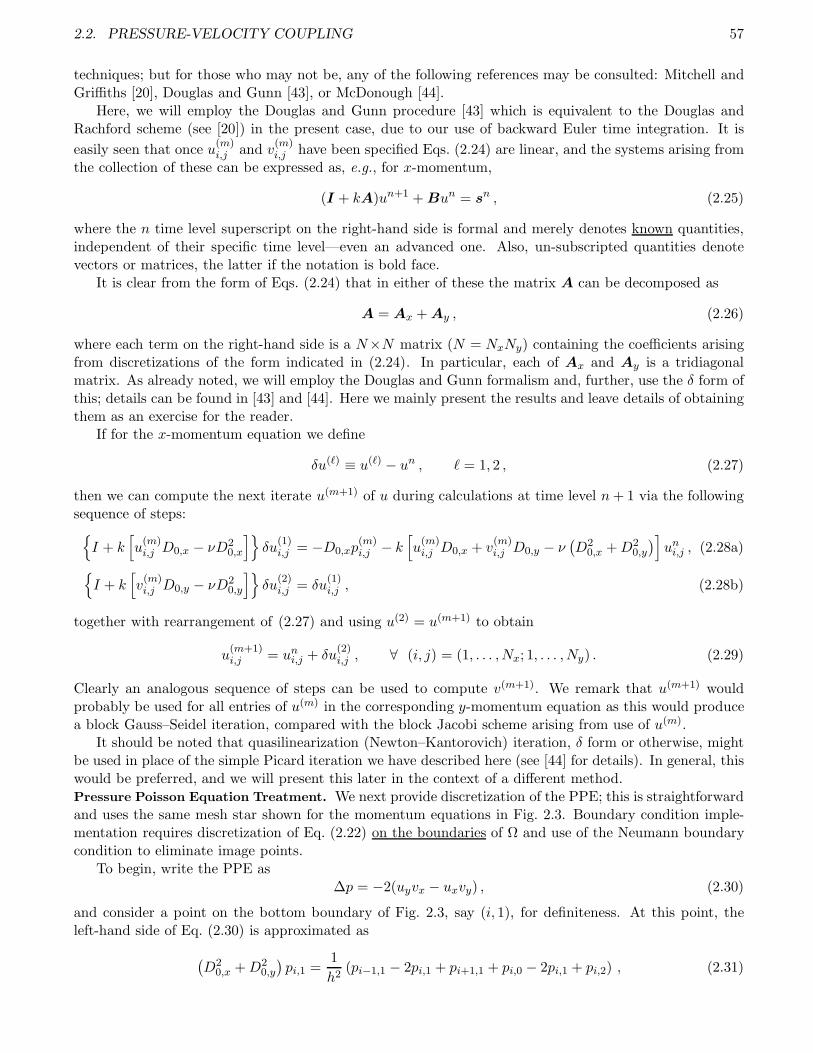
2.2. PRESSURE-VELOCITY COUPLING 57
techniques; but for those who may not be, any of the following references may be consulted: Mitchell andGriffiths [20], Douglas and Gunn [43], or McDonough [44].
Here, we will employ the Douglas and Gunn procedure [43] which is equivalent to the Douglas andRachford scheme (see [20]) in the present case, due to our use of backward Euler time integration. It is
easily seen that once u(m)i,j and v
(m)i,j have been specified Eqs. (2.24) are linear, and the systems arising from
the collection of these can be expressed as, e.g., for x-momentum,
(I + kA)un+1 + Bun = sn , (2.25)
where the n time level superscript on the right-hand side is formal and merely denotes known quantities,independent of their specific time level—even an advanced one. Also, un-subscripted quantities denotevectors or matrices, the latter if the notation is bold face.
It is clear from the form of Eqs. (2.24) that in either of these the matrix A can be decomposed as
A = Ax + Ay , (2.26)
where each term on the right-hand side is a N×N matrix (N = NxNy) containing the coefficients arisingfrom discretizations of the form indicated in (2.24). In particular, each of Ax and Ay is a tridiagonalmatrix. As already noted, we will employ the Douglas and Gunn formalism and, further, use the δ form ofthis; details can be found in [43] and [44]. Here we mainly present the results and leave details of obtainingthem as an exercise for the reader.
If for the x-momentum equation we define
δu(ℓ) ≡ u(ℓ) − un , ℓ = 1, 2 , (2.27)
then we can compute the next iterate u(m+1) of u during calculations at time level n+ 1 via the followingsequence of steps:I + k
[u
(m)i,j D0,x − νD2
0,x
]δu
(1)i,j = −D0,xp
(m)i,j − k
[u
(m)i,j D0,x + v
(m)i,j D0,y − ν
(D2
0,x +D20,y
)]un
i,j , (2.28a)
I + k
[v(m)i,j D0,y − νD2
0,y
]δu
(2)i,j = δu
(1)i,j , (2.28b)
together with rearrangement of (2.27) and using u(2) = u(m+1) to obtain
u(m+1)i,j = un
i,j + δu(2)i,j , ∀ (i, j) = (1, . . . ,Nx; 1, . . . ,Ny) . (2.29)
Clearly an analogous sequence of steps can be used to compute v(m+1). We remark that u(m+1) wouldprobably be used for all entries of u(m) in the corresponding y-momentum equation as this would producea block Gauss–Seidel iteration, compared with the block Jacobi scheme arising from use of u(m).
It should be noted that quasilinearization (Newton–Kantorovich) iteration, δ form or otherwise, mightbe used in place of the simple Picard iteration we have described here (see [44] for details). In general, thiswould be preferred, and we will present this later in the context of a different method.Pressure Poisson Equation Treatment. We next provide discretization of the PPE; this is straightforwardand uses the same mesh star shown for the momentum equations in Fig. 2.3. Boundary condition imple-mentation requires discretization of Eq. (2.22) on the boundaries of Ω and use of the Neumann boundarycondition to eliminate image points.
To begin, write the PPE as∆p = −2(uyvx − uxvy) , (2.30)
and consider a point on the bottom boundary of Fig. 2.3, say (i, 1), for definiteness. At this point, theleft-hand side of Eq. (2.30) is approximated as
(D2
0,x +D20,y
)pi,1 =
1
h2(pi−1,1 − 2pi,1 + pi+1,1 + pi,0 − 2pi,1 + pi,2) , (2.31)

58 CHAPTER 2. SPECIAL NUMERICAL DIFFICULTIES OF THE NAVIER–STOKES EQUATIONS
which contains a value of p at the image point (i, 0). On this boundary the homogeneous normal derivativeboundary condition is
∂p
∂n=∂p
∂y= 0 ,
which upon discretization with a centered difference implies that pi,0 = pi,2. Then substitution of this intothe right-hand side of (2.31) yields
1
h2(pi−1,1 − 4pi,1 + pi+1,1 + 2pi,2) ,
thus eliminating the image point.Similar results can be obtained for the remaining three boundaries, including corner points. We leave
demonstration of this as an exercise for the reader. We note at this point that the system matrix arisingfrom this discretization is nearly singular—theoretically, it is singular; but in machine arithmetic it missesbeing singular by the level of representation and rounding errors. Iterative solution methods perform verypoorly in this nearly-singular context.
We now consider treatment of the right-hand side of Eq. (2.30) on the boundaries of Ω. It should beclear that for the present problem, we have ux = vx = 0 at all horizontal boundary points, and similarlyuy = vy = 0 at vertical boundary points. At the same time, the right-hand side of Eq. (2.30) contains onex derivative and one y derivative in each term; hence, it is zero around the entire boundary. So no furtherattention need be given to the boundary treatment for this equation, and the basic problem discretizationis complete.
There is a final detail to consider before presenting a pseudo-language algorithm for solving the currentproblem. Recall that, as already noted, solutions to Neumann problems are not unique. Two mainapproaches have been used to address this numerically. The first, and less often used, is to set 〈p, 1〉 = 0.That is, at the end of the iterations associated with solving the PPE, we average the result and subtract theaverage value from the solution. The main difficulty with this approach is that it does nothing to improvethe performance of the iterative technique being used to solve the PPE. It is a satisfactory analyticalapproach that is of little value in practical computational procedures.
The second alternative entails assigning a value of pressure at one boundary point. Formally, this isequivalent to adding a constant value at all points, but since we do not yet know the pressure at any pointit does not matter whether we actually make the assignment anywhere except at the chosen boundarypoint. Once this has been done, the PPE problem becomes a mixed Dirichlet–Neumann one, possessing aunique solution and no longer exhibiting a singular coefficient matrix, although the condition number maystill be quite large. Thus, numerical solution procedures perform somewhat better. Moreover, adding aconstant in this way is of no other consequence since solutions to the original Neumann problem are uniqueonly to within an additive function of time in any case.
This completes the basic treatment required to formulate a pseudo-language algorithm; we present thisas follows.
Algorithm 2.1 (Basic unstaggered-grid treatment of N.–S. equations) Suppose n time steps (or pseudo-time steps, if a steady solution is being sought) have been completed. To advance the solution to time leveln+ 1, perform the following steps.
1. Do m1 = 1,maxpitrDo m2 = 1,maxitrsolve discrete x-momentum equations (2.28) with fixed p(m1)
solve discrete y-momentum equation analogous to (2.28) with fixed p(m1)
test convergence of velocity iterations:
If max(∥∥u(m2+1) − u(m2)
∥∥ ,∥∥v(m2+1) − v(m2)
∥∥) < ǫ, then go to 2Repeat m2
Write error message
2.2. PRESSURE-VELOCITY COUPLING 59
2. Solve PPEset pNx/2,1 = 0iteratively solve discretization of Eq. (2.30)test convergence of pressure iterations:
If(∥∥p(m1+1) − p(m1)
∥∥) < ǫ, then print resultsstop
else Repeat m1
3. Write error message
A few remarks are in order regarding details of the algorithm, per se, aside from those concerning theproblem formulation. First, the choice of solving the PPE in the outer loop is arbitrary, but preciselywhere this is done has little effect on the ultimate outcome. On the other hand, from a pure mathematicsstandpoint, it leads to difficulty in solving the momentum equations at the first time step since we are notpermitted to prescribe initial pressure independent of the velocity field. A simple remedy is to “create”initial data for pressure using initial velocity data to evaluate the right-hand side of Eq. (2.20). But thisimplies that the velocity field should be divergence free. An obvious alternative is to interchange steps 1and 2.
Second, the value of p chosen for the boundary assignment needed to produce a Dirichlet condition iscompletely arbitrary in the present problem, as should be clear from replacing p with p+C for any constantC in the PPE and Neumann conditions. Finally, the location on the grid at which this assignment is madeis also arbitrary in principle, but not completely so in practice. In particular, for centered approximations ofthe Laplacian, as employed herein, it is necessary to avoid the corners of a domain represented in Cartesiancoordinates because Dirichlet conditions at such points are never included in the discrete equations. It iscommon to make the Dirichlet condition assignment at a the midpoint of one of the sides of the domain,as done in the algorithm presented above.
Shortcomings of Basic Approach
As intuitively appealing as this algorithm might seem, it embodies many fundamental flaws renderingit incapable of producing correct numerical solutions to the N.–S. equations. For the most part these arerelated to the PPE and/or the divergence-free condition. We first list these, and then provide some furtherdetails.
i) The PPE is constructed under the assumption of satisfaction of the divergence-free constraint, butthere is no mechanism within the algorithm to guarantee this.
ii) Boundary conditions for the PPE are not generally correct—neither physically, nor mathematically.
iii) Centered finite-difference approximations on unstaggered grids permit discrete satisfaction of thedivergence-free constraint by non-physical velocity fields.
iv) Similarly, centered approximations to the pressure gradient terms (on unstaggered grids) in themomentum equations allow non-physical pressure fields to go “undetected”—and thus, uncorrected.
v) There exists a basic theorem from finite-element analysis of the N.–S. equations showing that useof centered approximations of both velocity and pressure, together, on an unstaggered grid will notconverge to a physically correct divergence-free solution.
We now present further details associated with each of these.
Failure to Explicitly Satisfy ∇·u = 0. With regard to the first item we note that although the divergence-free constraint has been employed to simplify the PPE, it (the constraint equation) has not been “solved.”Moreover, solutions to the momentum equations are not necessarily divergence free. (It they were, we would

60 CHAPTER 2. SPECIAL NUMERICAL DIFFICULTIES OF THE NAVIER–STOKES EQUATIONS
not need to separately impose the divergence-free constraint in the first place.) It is worth noting, however,that if initial data are divergence free, pressure is calculated correctly, and truncation and rounding errorsare negligible, then time evolution of such initial data preserves this property. It is well known that thiscan be accomplished for short times using spectral methods and high-precision machine arithmetic, buteventually the divergence-free property is lost.
Incorrect PPE Boundary Conditions. We next consider the boundary conditions required to solve thePPE, Eq. (2.30). It is often argued that at least in flow situations not too different from unseparatedboundary layers the condition
∂p
∂n= 0
might be adequate. (Indeed, it is often viewed as an “assumption”—but it is actually an outcome—inboundary-layer theory.) Here, we will show more precisely under what circumstances this is true, and thatit cannot be used in general. In the course of doing this we provide the correct boundary conditions.
To begin, we recall that to guarantee existence of solutions to Poisson/Neumann problems of the form
∆p = f in Ω (2.32)
with boundary conditions∂p
∂n= g on ∂Ω , (2.33)
the following consistency condition (or solvability condition), derived from the divergence theorem, mustbe satisfied (see, e.g., [27]): ∫
Ωf dx =
∫
∂Ωg dℓ , (2.34)
as noted earlier.Now recall that in constructing the PPE we started by taking the divergence of the momentum equa-
tions, and then simplified the result using the divergence-free condition. We begin in the same way here,but it is not useful to apply the divergence-free condition in this case because this arises as a vectoroperator, and here we will want to identify scalar boundary conditions. Thus, we write
−∇ · ∇p = ∇ · (ut + u · ∇u − ν∆u) ≡ f ,
but we do not carry out details of constructing the divergence. Instead, we nowapply the divergencetheorem to see that ∫
Ω∇ · ∇p dx =
∫
∂Ωn · ∇p dℓ ,
and at the same time we have (by using the N.–S. equations on the right-hand side)
∫
Ω∇ · ∇p dx = −
∫
Ω∇ · (ut + u · ∇u − ν∆u) dx =
∫
Ωf dx
= −∫
∂Ωn · (ut + u · ∇u − ν∆u) dℓ
(≡∫
∂Ωg dℓ
),
with the divergence theorem used to obtain the equality in the second line. Thus, we see that the consistencyrequirement is automatically satisfied if on vertical boundaries we set
∂p
∂x= − (ut + uux + vuy − ν∆u) , (2.35)
and on horizontal boundaries we use
∂p
∂y= − (vt + uvx + vvy − ν∆v) , (2.36)

2.2. PRESSURE-VELOCITY COUPLING 61
as proposed by Gresho and Sani [30]. In this way we have prescribed functions g that automatically satisfy(2.34).
It is of interest at this point to see under what conditions the above essentially collapse to the homo-geneous Neumann conditions that are often used. First, it is clear that the boundary values of u must beindependent of time. Furthermore, if u and v are both zero on all boundaries, then the only remainingterms are ν∆u on vertical boundaries and ν∆v on horizontal ones. (We remark that such a combinationof velocity boundary conditions will require that body forces be acting to drive the flow unless there is theadditional complication of inflow and outflow.) In any case, under these assumed conditions we see thatas ν → 0 (or, equivalently, as Re→ ∞), the above general conditions collapse to
∂p
∂x≃ 0 , and
∂p
∂y≃ 0 .
Effects of Centered Differencing of Continuity Equation. We next consider the effects of centered differ-encing with respect to satisfaction of the continuity equation. In particular, we will show that completelynon-physical velocity fields are able to satisfy the discrete divergence-free condition obtained by centereddifferencing. We begin by considering the simple 1-D case for which the divergence-free condition collapsesto ux = 0. This, of course, implies u ≡ const. But in Fig. 2.4 we display a non-constant grid function uithat satisfies D0,xui = 0.
=u
−i 1 +i 1
2 2 2 21 1 1 1 12
ih
Figure 2.4: Non-constant grid function satisfying discrete 1-D continuity equation.
The same situation occurs also in 2D and 3D. We illustrate this here for the former case, and leave asimilar construction in 3D for the reader. Now the discrete divergence-free constraint is
D0,xui,j +D0,yvi,j = 0 ,
or with hx = hy = h,
ui+1,j − ui−1,j + vi,j+1 − vi,j−1 = 0 . (2.37)
Figure 2.5 presents a velocity field that exactly satisfies Eq. (2.37), but which makes no physical sense. Thereader can easily check that Eq. (2.37) is satisfied at all interior grid points. Clearly, somewhat unrealisticboundary conditions would be needed to produce this uniform distribution of values, and in practice theeffect is not so perfectly obtained. Nevertheless, it is observed in significant regions of a domain for actualcalculations carried out with centered-difference approximations on unstaggered and partially-staggeredgrids.
For reasons that should be obvious from the figure, this phenomenon is termed “checkerboarding.”It is interesting to note that in the extreme case depicted in Fig. 2.5 the right-hand side of the usualdiscrete PPE would be zero. Together with homogeneous Neumann boundary conditions this would resultin a constant pressure field, so its use in the discrete momentum equations would have no effect on thecomputed velocity field. We see from this that once it occurs, the checkerboard solution is very stable andcannot easily be corrected.
It is clear from Fig. 2.5 that if we were to employ first-order forward differencing to approximate thecontinuity equation, the checkerboard solution shown here would not be discretely divergence free. On theother hand, if we were to use a combination of forward and backward differences such as
D+,xui,j +D−,yvi,j = 0 ,

62 CHAPTER 2. SPECIAL NUMERICAL DIFFICULTIES OF THE NAVIER–STOKES EQUATIONS
hy
hx
1,3 2,4 1,3 1,32,4
1,3 2,4 1,3 1,32,4
2,4 1,3 2,4 1,3 2,4
i,j
u,v = 1,3 2,4 1,3 1,32,4
2,4 1,3 2,4 1,3 2,4
( )
Figure 2.5: Non-physical grid function satisfying discrete 2-D continuity equation.
we would recover satisfaction of the discrete divergence-free constraint. This suggests that use of low-order, one-sided difference approximations, as has sometimes been proposed, will not necessarily correctthe problem.Centered Approximation of Pressure Gradient in Momentum Equations. It can also be seen thatcentered approximations to the pressure-gradient terms of the momentum equations are unable to correcta checkerboard phenomenon. For example, consider the pressure field exhibited in Fig. 2.6. Clearly, once
hy
hx
p = 1 2 1 2 1
1 2 1 2 1
1 2 1 2 1
1 2 1 2 1
1 2 1 2 1
i,j( )
Figure 2.6: Non-physical checkerboard pressure distribution.
this pressure field exists, it can no longer act to modify the velocity field that may have been responsiblefor creating it in the first place because the centered discretizations representing the pressure gradient,D0,xpi,j and D0,ypi,j, produce identically zero results for both components, and the momentum equationscan no longer effect changes to this velocity distribution.
The Div-Stability Condition. The last main issue with the current algorithm to be considered here is inmany ways the most important, and at the same time the least well known and understood. In finite-elementanalysis of the Navier–Stokes equations there is a condition known as the Ladyzhenskaya–Babuska–Brezzi(LBB) condition, more recently termed the div-stability condition (see Gunzburger [45] and referencestherein), whose satisfaction guarantees that associated finite-element spaces for velocity and pressure aresuch that divergence-free finite-element approximations converge to divergence-free exact solutions as theelement size approaches zero. Details of this condition are technically difficult; moreover, the condition is

2.2. PRESSURE-VELOCITY COUPLING 63
not easily checked for general practical situations. As a consequence we will not present the mathematicalrepresentation of the condition, itself, but rather list some well-known and important consequences. Theseare as follows:
i) the combination of centered finite-difference approximation and unstaggered gridding does not satisfythe div-stability condition;
ii) in general, for finite-element methods it is necessary either to use different degree polynomial ap-proximations for velocity and pressure (so-called mixed finite elements) on the same mesh, or to usethe same degree and different meshes (staggered grid) in order to satisfy the div-stability condition;
iii) in the finite-element context, satisfaction of the div-stability requirement can be circumvented viamodifications to the discrete continuity equation.
We note that ii) can be taken to imply that staggered grids should be used in the finite-differencecontext if the same order of accuracy is to be used in approximating both velocity and pressure. Inaddition, within the confines of finite-difference approximations iii) implies that modifications to the PPE(or other equations for pressure—see the artificial compressibilty method in Chap. 3) might be made topermit calculations on unstaggered grids, or from ii), a lower order of accuracy might be employed forpressure calculations.
Finite-Volume Discretization of the N.–S. Equations on Staggered Grids
In this subsection we present a detailed analysis of finite-volume discretization of the N.–S. equationson a staggered grid. We note that, in principle, this is equivalent to a finite-difference approximation;indeed, the final results will be identical. But the finite-volume derivation is useful in its own right, andin addition it actually provides the motivation for specific point location, and dependent variable location,assignments on the staggered grid. Hence, we will emphasize it here. We begin with discretization of thecontinuity equation which requires dependent variable assignments at grid locations different from thoseof the natural finite-difference grid points; so this permits us to set up the staggered-grid formalism in thesimplest possible situation. We follow this with a corresponding treatment of the x-momentum equationand an abbreviated analysis of the y-momentum equation, and we conclude by briefly describing boundarycondition implementations.
Continuity Equation. Consider the continuity equation (divergence-free constraint) in 2D,
∇ · u = ux + vy = 0 , (2.38)
on a single grid cell, denoted Ωi,j and displayed in Fig. 2.7. As the figure shows, this cell is defined asthe region bounded by the i − 1 and i grid lines in the x-direction, and by the j − 1 and j lines in they-direction. These are separated by the grid spacings hx and hy, respectively. On each such cell we musthave ∫
Ωi,j
∇ · u dV = 0
(since Eq. (2.38) holds at every point in the continuum), and from Gauss’s theorem we obtain
∫
∂Ωi,j
u · n dA = 0 ,
or ∫
∂Ωi,j
unx + v ny dA = 0 . (2.39)
Here, the differential elements dV and dA correspond to the 3-D case, but we will retain this notation herein 2D where they actually imply area and arclength, respectively.

64 CHAPTER 2. SPECIAL NUMERICAL DIFFICULTIES OF THE NAVIER–STOKES EQUATIONS
Figure 2.7: Staggered grid cell, Ωi,j.
If we let u denote the average velocity through a vertical segment of ∂Ωi,j and let v be the averagethrough horizontal segments we can evaluate (2.39) as
(ui − ui−1)hy + (vj − vj−1)hx = 0 , (2.40)
with single indices denoting the associated face of Ωi,j. But it is convenient to view these averages assimply being values at the center of the corresponding cell faces (which they are as the discretization stepsizes approach zero). So, by using the notation of Fig. 2.7, we can write Eq. (2.40) as
1
hx
(ui,j−1/2 − ui−1,j−1/2
)+
1
hy
(vi−1/2,j − vi−1/2,j−1
)= 0 . (2.41)
It should be noted that this is a centered approximation to the divergence-free constraint, but one usingonly a single grid cell rather than the usual four cells that would be needed in the context of unstaggeredgridding. We leave demonstration of second-order accuracy of this approximation as an exercise for thereader.
Now with this representation of the continuity equation it is natural to locate the associated pressureat the cell center, as indicated in Fig. 2.7. In particular, recall that pressure must be determined so as tosatisfy the divergence-free constraint expressed here as Eq. (2.41), and the grid location (i− 1/2, j − 1/2)is closest to (in fact, equidistant from, if hx = hy) all of the grid locations used in (2.41). Indeed, it isthe location at which the divergence is being calculated, as is clear from Eq. (2.41); thus, it should be thepreferred location for p.
Momentum Equations. Having established a rationale for grid function locations within a grid cell, wecan now proceed to the more complicated derivation of the finite-volume form of the momentum equations.We will carry this out in detail for the x-momentum equation and merely outline steps and give the resultfor y-momentum, leaving the details of obtaining this as an exercise for the reader.
We start with the vector form of the equations (in the absence of body forces),
Du
Dt= −∇p+ ν∇·∇u ,
2.2. PRESSURE-VELOCITY COUPLING 65
which we integrate over the grid cell Ωi,j:
∫
Ωi,j
Du
DtdV =
∫
Ωi,j
−∇p+ ν∇·∇udV .
Application of the divergence theorem to the right-hand side results in
∫
Ωi,j
Du
DtdV =
∫
∂Ωi,j
−pn + ν∇u·n dA ,
and we write this in component form as
∫
Ωi,j
D
Dt
(uv
)dV =
∫
∂Ωi,j
−(pnx
pny
)+ ν
(uxnx + uyny
vxnx + vyny
)dA . (2.42)
We now consider the x-component of this,
∫
Ωi,j
∂u
∂t+ u·∇u dV =
∫
∂Ωi,j
−pnx + ν(uxnx + uyny) dA , (2.43)
in detail. By assuming the problem geometry and grid configuration are independent of time we cancommute differentiation and integration in the first term on the left-hand side, and after applying Gauss’stheorem to the second term on the left, we obtain
∂
∂t
∫
Ωi,j
u dV +
∫
∂Ωi,j
u2nx + vuny dA =
∫
∂Ωi,j
−pnx + ν(uxnx + uyny) dA . (2.44)
Here, we have used u·∇u = ∇·(uu) (which follows from the divergence-free constraint) in order to obtaina form to which Gauss’s theorem applies. (Observe that this step automatically produces the conservationform of the momentum equations.)
The next step is to evaluate each of the terms in Eq. (2.44) on the grid cell shown in Fig. 2.8. Weemphasize that this is not the same grid cell utilized in the analysis of the continuity equation. Indeed,when working with a staggered grid it is necessary to define separate grid cells for each of the momentumequations, and for the continuity equation; pressure, and all other scalar quantities, use the same grid cellas that employed for the continuity equation. We observe that the grid cell displayed in Fig. 2.8 is centeredon the location of the x-component of velocity at the ith grid line. The vertical cell walls correspond tolocations i− 1/2 and i+ 1/2, and horizontal cell walls coincide with the j − 1 and j grid lines. There aretwo main factors motivating this choice of cell boundaries. First, accurate evaluation of the first term onthe left-hand side of Eq. (2.44) is simpler if the velocity component is at the cell center. Second, becausepressure is often viewed, physically, as the main driving force in the momentum equations (in the absenceof body forces), it is natural to define pressure on cell walls—pressure produces a surface force, so thenatural place to represent it is on a cell boundary. We remark that this is completely analogous to thecontrol-volume analyses learned in elementary fluid dynamics courses, but there the control volume wouldusually be of macroscopic size, rather than the grid cell used here that in principle will be allowed to goto zero area or volume.
In terms of the grid cell shown in Fig. 2.8 it is clear that the first term in Eq. (2.44) can be evaluatedas
∂
∂t
∫
Ωi,j
u dV =∂
∂tui,j−1/2hxhy , (2.45)
under the assumption that ui,j−1/2 is the average x-component velocity within the cell. We note that sinceui,j−1/2 is cell centered, spatial integration over the grid cell presented in Fig. 2.8 corresponds to midpointquadrature, and thus is third-order accurate, locally.
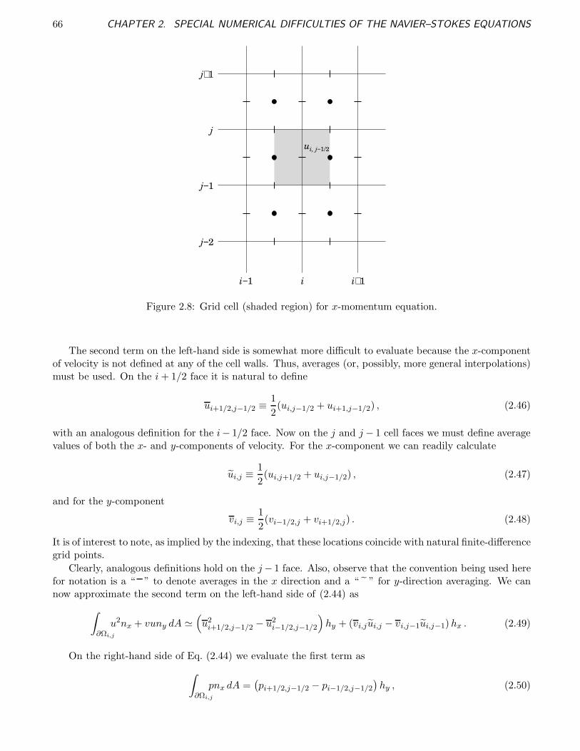
66 CHAPTER 2. SPECIAL NUMERICAL DIFFICULTIES OF THE NAVIER–STOKES EQUATIONS
ui, j−1/2
i−1 i i+1
j−2
j−1
j
j+1
Figure 2.8: Grid cell (shaded region) for x-momentum equation.
The second term on the left-hand side is somewhat more difficult to evaluate because the x-componentof velocity is not defined at any of the cell walls. Thus, averages (or, possibly, more general interpolations)must be used. On the i+ 1/2 face it is natural to define
ui+1/2,j−1/2 ≡ 1
2(ui,j−1/2 + ui+1,j−1/2) , (2.46)
with an analogous definition for the i− 1/2 face. Now on the j and j − 1 cell faces we must define averagevalues of both the x- and y-components of velocity. For the x-component we can readily calculate
ui,j ≡1
2(ui,j+1/2 + ui,j−1/2) , (2.47)
and for the y-component
vi,j ≡1
2(vi−1/2,j + vi+1/2,j) . (2.48)
It is of interest to note, as implied by the indexing, that these locations coincide with natural finite-differencegrid points.
Clearly, analogous definitions hold on the j− 1 face. Also, observe that the convention being used herefor notation is a “ ” to denote averages in the x direction and a “ ˜ ” for y-direction averaging. We cannow approximate the second term on the left-hand side of (2.44) as
∫
∂Ωi,j
u2nx + vuny dA ≃(u2
i+1/2,j−1/2 − u2i−1/2,j−1/2
)hy + (vi,jui,j − vi,j−1ui,j−1)hx . (2.49)
On the right-hand side of Eq. (2.44) we evaluate the first term as
∫
∂Ωi,j
pnx dA =(pi+1/2,j−1/2 − pi−1/2,j−1/2
)hy , (2.50)
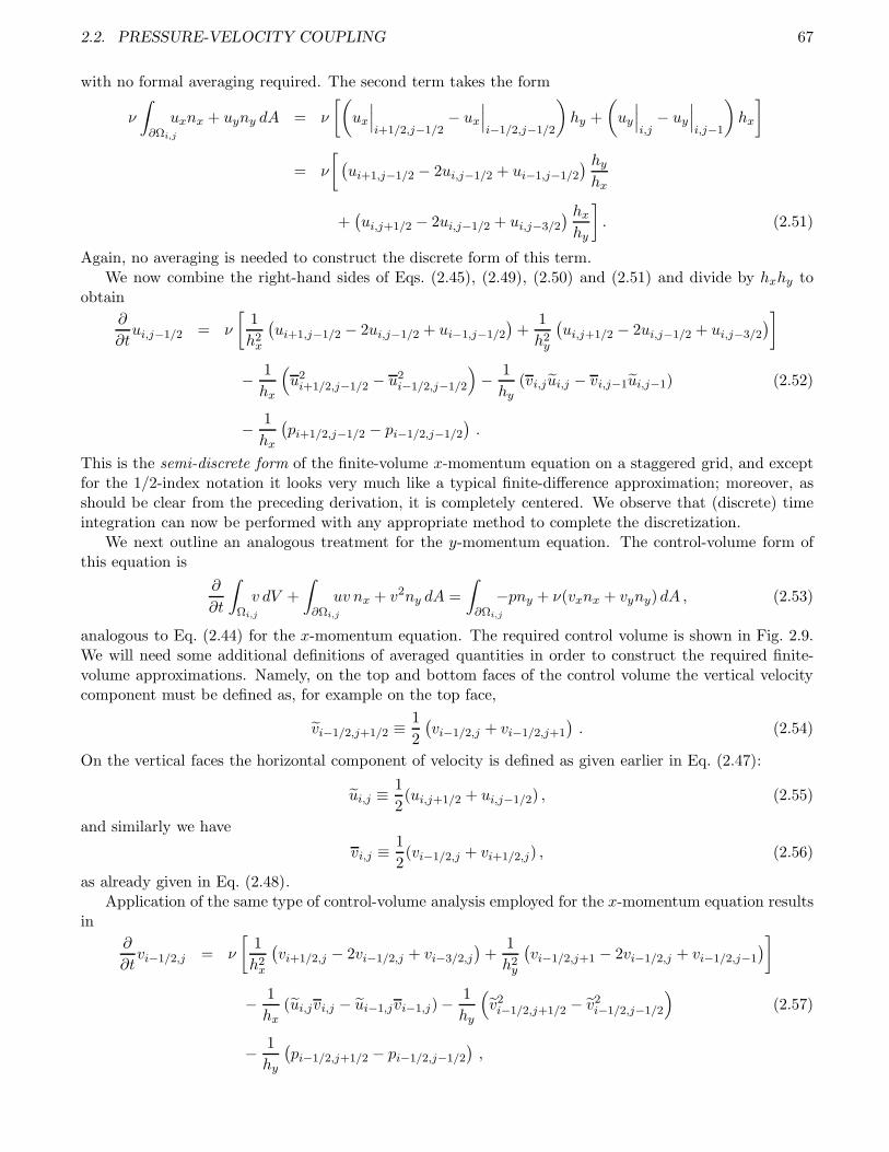
2.2. PRESSURE-VELOCITY COUPLING 67
with no formal averaging required. The second term takes the form
ν
∫
∂Ωi,j
uxnx + uyny dA = ν
[(ux
∣∣∣i+1/2,j−1/2
− ux
∣∣∣i−1/2,j−1/2
)hy +
(uy
∣∣∣i,j
− uy
∣∣∣i,j−1
)hx
]
= ν
[ (ui+1,j−1/2 − 2ui,j−1/2 + ui−1,j−1/2
) hy
hx
+(ui,j+1/2 − 2ui,j−1/2 + ui,j−3/2
) hx
hy
]. (2.51)
Again, no averaging is needed to construct the discrete form of this term.We now combine the right-hand sides of Eqs. (2.45), (2.49), (2.50) and (2.51) and divide by hxhy to
obtain
∂
∂tui,j−1/2 = ν
[1
h2x
(ui+1,j−1/2 − 2ui,j−1/2 + ui−1,j−1/2
)+
1
h2y
(ui,j+1/2 − 2ui,j−1/2 + ui,j−3/2
)]
− 1
hx
(u2
i+1/2,j−1/2 − u2i−1/2,j−1/2
)− 1
hy(vi,jui,j − vi,j−1ui,j−1) (2.52)
− 1
hx
(pi+1/2,j−1/2 − pi−1/2,j−1/2
).
This is the semi-discrete form of the finite-volume x-momentum equation on a staggered grid, and exceptfor the 1/2-index notation it looks very much like a typical finite-difference approximation; moreover, asshould be clear from the preceding derivation, it is completely centered. We observe that (discrete) timeintegration can now be performed with any appropriate method to complete the discretization.
We next outline an analogous treatment for the y-momentum equation. The control-volume form ofthis equation is
∂
∂t
∫
Ωi,j
v dV +
∫
∂Ωi,j
uv nx + v2ny dA =
∫
∂Ωi,j
−pny + ν(vxnx + vyny) dA , (2.53)
analogous to Eq. (2.44) for the x-momentum equation. The required control volume is shown in Fig. 2.9.We will need some additional definitions of averaged quantities in order to construct the required finite-volume approximations. Namely, on the top and bottom faces of the control volume the vertical velocitycomponent must be defined as, for example on the top face,
vi−1/2,j+1/2 ≡ 1
2
(vi−1/2,j + vi−1/2,j+1
). (2.54)
On the vertical faces the horizontal component of velocity is defined as given earlier in Eq. (2.47):
ui,j ≡1
2(ui,j+1/2 + ui,j−1/2) , (2.55)
and similarly we have
vi,j ≡1
2(vi−1/2,j + vi+1/2,j) , (2.56)
as already given in Eq. (2.48).Application of the same type of control-volume analysis employed for the x-momentum equation results
in
∂
∂tvi−1/2,j = ν
[1
h2x
(vi+1/2,j − 2vi−1/2,j + vi−3/2,j
)+
1
h2y
(vi−1/2,j+1 − 2vi−1/2,j + vi−1/2,j−1
)]
− 1
hx(ui,jvi,j − ui−1,jvi−1,j) −
1
hy
(v2i−1/2,j+1/2 − v2
i−1/2,j−1/2
)(2.57)
− 1
hy
(pi−1/2,j+1/2 − pi−1/2,j−1/2
),
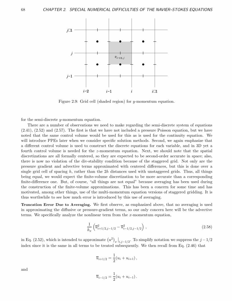
68 CHAPTER 2. SPECIAL NUMERICAL DIFFICULTIES OF THE NAVIER–STOKES EQUATIONS
i−1 i i+1i−2
j−1
j
j+1
vi−1/2, j
Figure 2.9: Grid cell (shaded region) for y-momentum equation.
for the semi-discrete y-momentum equation.
There are a number of observations we need to make regarding the semi-discrete system of equations(2.41), (2.52) and (2.57). The first is that we have not included a pressure Poisson equation, but we havenoted that the same control volume would be used for this as is used for the continuity equation. Wewill introduce PPEs later when we consider specific solution methods. Second, we again emphasize thata different control volume is used to construct the discrete equations for each variable, and in 3D yet afourth control volume is needed for the z-momentum equation. Next, we should note that the spatialdiscretizations are all formally centered, so they are expected to be second-order accurate in space; also,there is now no violation of the div-stability condition because of the staggered grid. Not only are thepressure gradient and advective terms approximated with centered differences, but this is done over asingle grid cell of spacing h, rather than the 2h distances used with unstaggered grids. Thus, all thingsbeing equal, we would expect the finite-volume discretization to be more accurate than a correspondingfinite-difference one. But, of course, “all things are not equal” because averaging has been used duringthe construction of the finite-volume approximations. This has been a concern for some time and hasmotivated, among other things, use of the multi-momentum equation versions of staggered gridding. It isthus worthwhile to see how much error is introduced by this use of averaging.
Truncation Error Due to Averaging. We first observe, as emphasized above, that no averaging is usedin approximating the diffusive or pressure-gradient terms, so our only concern here will be the advectiveterms. We specifically analyze the nonlinear term from the x-momentum equation,
1
hx
(u2
i+1/2,j−1/2 − u2i−1/2,j−1/2
), (2.58)
in Eq. (2.52), which is intended to approximate(u2)x
∣∣i,j−1/2
. To simplify notation we suppress the j−1/2
index since it is the same in all terms to be treated subsequently. We then recall from Eq. (2.46) that
ui+1/2 =1
2(ui + ui+1) ,
and
ui−1/2 =1
2(ui + ui−1) .
2.2. PRESSURE-VELOCITY COUPLING 69
We next note that for uniform grid spacing, hx = h,
ui = ui+1/2 −h
2u′i+1/2 +
h2
8u′′i+1/2 + · · · ,
ui+1 = ui+1/2 +h
2u′i+1/2 +
h2
8u′′i+1/2 + · · · ,
which implies that
ui+1/2 = ui+1/2 +h2
8u′′i+1/2 + · · · ,
where “ ′ ” denotes differentiation (with respect to x in this case). Similarly, we obtain
ui−1/2 = ui−1/2 +h2
8u′′i−1/2 + · · · .
Substitution of the expansions for ui+1/2 and ui−1/2 into (2.58) results in
1
hx
(u2
i+1/2 − u2i−1/2
)=
1
hx
(u2
i+1/2 − u2i−1/2
)+h2
x
4
[1
hx
(ui+1/2u
′′i+1/2 − ui−1/2u
′′i−1/2
)]
+h4
x
64
[1
hx
(u′′i+1/2 − u′′i−1/2
)]+ · · · ,
=(u2)x
∣∣∣∣i
+h2
x
4(uuxx)x
∣∣∣∣i
+ O(h4x) . (2.59)
It is easily checked that the O(h2) term on the right-hand side of this expression is of exactly the sameform as the dominant truncation error term of a conserved-form centered-difference approximation usingthe natural finite-difference grid points i− 1 and i+ 1, but it is actually smaller. In particular, the latteris h2
3 uuxxx + h2uxuxx, so each term of this is larger than the corresponding term in the staggered-gridfinite-volume approximation, the second term on the right-hand side of Eq. (2.59) after expansion bydifferentiation. Thus, we see that the combination of averaging and then differencing over an interval halfthe usual size actually reduces the error, and concerns that have been raised regarding effects of averagingare probably unwarranted—at least in many situations. Moreover, we observe that the truncation errorexpansions contain only even powers of h; hence, Richardson extrapolation will be effective for improvingaccuracy. We leave as an exercise for the reader the task of comparing the corresponding errors in bilinearterms such as (uv)y and the nonlinear term (v2)y from the y-momentum equation.
Notation and Implementation Considerations. As we have already noted, the staggered-grid formulationrequires use of three separate control volumes in 2D (four in 3D), and in addition to this the one-halfindexing is very inconvenient from the standpoint of coding and implementation. There is little doubt thatthese problems played at least some role in the use of the “NESW indexing” that has been widely used inCFD at least since introduction of the SIMPLE algorithm by Patankar, which we will study in detail inthe next chapter. But this notation does not extend in any natural way to 3D, and it is difficult (but, ofcourse, not impossible) to use for any but the simplest discretizations. Here we intoduce an approach thatremoves the problem of one-half indices without requiring storage of every point of the staggered grid. Inparticular, we will demonstrate how to employ “cell” notation and storage instead of the usual grid-pointnotation (and storage). In light of the fact that our discretizations have been constructed on grid cells viacontrol-volume analysis on each such cell, this will be a natural approach. We note that it had first beenintroduced (using different notation) at least by the time of publication of Patankar’s book [40].
Figure 2.10 provides a schematic of the notation, and a motivation for this approach in terms of thethree overlapping staggered-grid control volumes. In this figure we display with dashed lines the threecontrol volumes treated earlier, and we also indicate a mesh star associated with the collection of staggered

70 CHAPTER 2. SPECIAL NUMERICAL DIFFICULTIES OF THE NAVIER–STOKES EQUATIONS
i−1i−2 i i+1
j−2
j−1
j
j+1
(i,j) grid cellth
x momentum
y momentum
pressure, divergence
u
v
p
v
u
Figure 2.10: Grid-cell indexing.
points, one from the center of each of the three control volumes, corresponding to the dependent variablesassociated with the grid cell (i, j), i.e., Ωi,j. (Observe that the cell multi index corresponds to that ofthe natural finite-difference grid point in the upper right-hand corner of the cell.) We remark that thisconfiguration is not the only possible one, as the reader will quickly recognize, but in general all otheralternatives are of no more (or less) utility than the one shown; and this one is widely used.
The important point to observe is that with this change of indexing, ui,j−1/2 7−→ ui,j , vi−1/2,j 7−→ vi,j,and pi−1/2,j−1/2 7−→ pi,j, corresponding to the indicated mesh star, all cell values of dependent variablesare taken into account as i and j are ranged over the total set of grid cells. Moreover, there is no extrastorage needed in simple implementations beyond the one storage location per dependent variable, per gridcell—precisely the same as for an unstaggered grid. Finally, we can express the difference approximationsobtained earlier as Eqs. (2.41), (2.52) and (2.57) in the non-fractional index notation as follows.
Continuity (divergence-free constraint):
1
hx(ui,j − ui−1,j) +
1
hy(vi,j − vi,j−1) = 0 (2.60)
2.2. PRESSURE-VELOCITY COUPLING 71
Momentum equations (Newton’s second law of motion):
∂
∂tui,j = ν
[1
h2x
(ui+1,j − 2ui,j + ui−1,j) +1
h2y
(ui,j+1 − 2ui,j + ui,j−1)
]
− 1
hx(pi+1,j − pi,j) −
1
hx
(u2
i+1,j − u2i,j
)− 1
hy(vi,jui,j − vi,j−1ui,j−1) , (2.61a)
∂
∂tvi,j = ν
[1
h2x
(vi+1,j − 2vi,j + vi−1,j) +1
h2y
(vi,j+1 − 2vi,j + vi,j−1)
]
− 1
hy(pi,j+1 − pi,j) −
1
hx(ui,jvi,j − ui−1,jvi−1,j) −
1
hy
(v2i,j+1 − v2
i,j
). (2.61b)
The various averaged quantities used in these equations are now defined in terms of integer indices as
ui,j =1
2(ui,j + ui−1,j) , (2.62a)
vi,j =1
2(vi,j + vi+1,j) , (2.62b)
ui,j =1
2(ui,j + ui,j+1) , (2.62c)
vi,j =1
2(vi,j + vi,j−1) . (2.62d)
We comment that, at face value, the various approximations of first derivative terms appear to correspondto first-order accurate forward and backward differences, so it is important to recognize that this is onlynotation, and not the actual form (centered with step size h) of the difference approximations.
A final note is needed here with regard to implementation. Namely, most CFD post-processing tools(e.g., FieldView and TecPlot) construct their displays based on unstaggered, natural grid-point locations.Thus, computed results from staggered (and also from cell-centered unstaggered) grids must be interpolatedto these cell-vertex locations. Clearly, there are many possible approaches for doing this, and we leaveselection of any specific one to the reader. We observe, however, that in practice very simple multi-linearinterpolations are often employed, for good or for ill—even in commercial software.
Implementation of Boundary Conditions on Staggered Grids. Now that we have a practical indexingsystem at our disposal we can consider the final topic of this section, implementation of boundary condi-tions in the context of staggered-grid discretizations. Figure 2.11 displays a neighborhood of the bottomhorizontal boundary of a computational domain. We will consider boundary conditions for x- and y-momentum equations and the pressure Poisson equation at the grid cell Ωi,2. Analogous treatments can beconstructed on all other boundaries, and for other equations associated with any specific physical problem(e.g., thermal energy or species concentration).
Since the grid line j = 1 coincides with the actual physical boundary, we observe that the no-slipcondition for the x-momentum equation cannot be exactly satisfied, as we have noted earlier. In particular,this condition must be applied at the natural finite-difference grid point indicated with a solid square in thefigure, i.e., on the physical boundary. It is patently incorrect to attempt to impose the no-slip conditionfor the x-momentum equation at the point corresponding to the u-component of velocity in the (i, 2) gridcell.
But it is clear that required discretizations in the y direction at this point will involve the u-componentimage point (i, 1) whose value is unknown. Hence, in addition to attempting to satisfy a boundary conditionat a point that is not even a part of the calculation, we will in any case need a grid-point value at a pointoutside the solution (and physical) domain for which we have no governing equation. Fortunately, theremedy for both of these difficulties is the same—and it is well known.
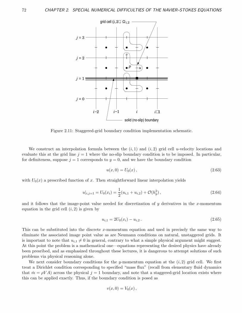
72 CHAPTER 2. SPECIAL NUMERICAL DIFFICULTIES OF THE NAVIER–STOKES EQUATIONS
j = 0
j = 1
j = 2
j = 3
i−2 i−1 i i+1
solid (no-slip) boundary
grid cell (i,2), Ω i,2
u
v
p
Figure 2.11: Staggered-grid boundary condition implementation schematic.
We construct an interpolation formula between the (i, 1) and (i, 2) grid cell u-velocity locations andevaluate this at the grid line j = 1 where the no-slip boundary condition is to be imposed. In particular,for definiteness, suppose j = 1 corresponds to y = 0, and we have the boundary condition
u(x, 0) = U0(x) , (2.63)
with U0(x) a prescribed function of x. Then straightforward linear interpolation yields
u|i,j=1 = U0(xi) =1
2(ui,1 + ui,2) + O(h2
y) , (2.64)
and it follows that the image-point value needed for discretization of y derivatives in the x-momentumequation in the grid cell (i, 2) is given by
ui,1 = 2U0(xi) − ui,2 . (2.65)
This can be substituted into the discrete x-momentum equation and used in precisely the same way toeliminate the associated image point value as are Neumann conditions on natural, unstaggered grids. Itis important to note that ui,1 6= 0 in general, contrary to what a simple physical argument might suggest.At this point the problem is a mathematical one—equations representing the desired physics have alreadybeen presribed, and as emphasized throughout these lectures, it is dangerous to attempt solutions of suchproblems via physical reasoning alone.
We next consider boundary conditions for the y-momentum equation at the (i, 2) grid cell. We firsttreat a Dirichlet condition corresponding to specified “mass flux” (recall from elementary fluid dynamicsthat m = ρV A) across the physical j = 1 boundary, and note that a staggered-grid location exists wherethis can be applied exactly. Thus, if the boundary condition is posed as
v(x, 0) = V0(x) ,
2.2. PRESSURE-VELOCITY COUPLING 73
then the associated numerical boundary condition is
v|i,j=1 = V0(xi) .
But because the numerical boundary point in this case coincides with the physical boundary, these valuescan be assigned in the usual way, with no approximation. Moreover, the difference approximation to they-momentum equation is first employed in the (i, 2) cell because the boundary condition is of Dirichlettype. The y-direction discretization will include the point at (i, 1), and the value of V0(xi) can be directlysubstituted for the corresponding grid-function value.
Just as the Dirichlet conditions are handled in the usual way for the y-momentum/horizontal boundarycase, so also are Neumann conditions. In this situation it is clear that the boundary at j = 1 cannot besolid. Furthermore, as is always the case with Neumann boundary conditions, the differential equationmust be solved on the boundary. It is easily seen that the corresponding discretization will include a grid-point value on the j = 0 line, i.e., an image-point value. But the Neumann condition, when discretized inthe usual way, will contain this same value; so it can be eliminated in a manner that is identical to thatused in the same circumstance on a natural, unstaggered grid.
Finally, we consider the PPE. In the case of solid boundaries we have already seen that the correctboundary condition for the present case is Eq. (2.36), which we repeat here:
∂p
∂y= −(vt + uvx + vvy − ν∆v) . (2.66)
For definiteness we suppose v ≡ 0 (i.e., a homogeneous Dirichlet condition) holds on the j = 1 boundary,and we leave as an exercise for the interested reader the task of identifying and treating other cases.
We first consider the left-hand side of this equation. The PPE, itself, will have been discretized in thegrid cell (i, 2), but not in general in the image cell (i, 1). Approximation of ∂2p/∂y2 in the usual way thenleads to
1
h2y
(pi,1 − 2pi,2 + pi,3) ,
and pi,1 must be determined from the Neumann boundary condition.Now just as was true for the x-momentum equation, the grid points for pressure do not occur on the
horizontal boundary (in fact, for pressure, they do not coincide with any boundaries), but the Neumanncondition must be applied on the physical boundary, i.e., at j = 1. This implies that ∂p/∂y|i,j=1 shouldbe approximated as
∂p
∂y
∣∣∣∣i,j=1
=1
hy(pi,2 − pi,1) , (2.67)
showing that pi,1 can be expressed in terms of pi,2 in order to eliminate it from the difference equation forthe latter.
What remains is to treat the right-hand side of Eq. (2.66). In the specific case of v ≡ 0 on the boundary,as being considered here, it is clear that vt ≡ 0, and vx ≡ 0. Thus, the only nonzero term in the right-handside of (2.66) is ν∂2v/∂y2. Because of the Dirichlet condition applied to the y-momentum equation inthis case, there is no image-point value available with which to construct a centered approximation on theboundary in any direct way, except to first perform an extrapolation. A typically-better alternative is toemploy a one-sided difference approximation. This can be done to maintain second-order accuracy withthe following discretization:
∂2v
∂y2=
1
h2y
(2vi,1 − 5vi,2 + 4vi,3 − vi,4) + O(h2
y
)(2.68)
with vi,1 ≡ 0 in the present case. Although this appears somewhat complicated, it does not pose any seriousdifficulties because vi,j will already have been determined prior to its use in a boundary condition forpressure of the form Eq. (2.66).

74 CHAPTER 2. SPECIAL NUMERICAL DIFFICULTIES OF THE NAVIER–STOKES EQUATIONS
The final case of boundary conditions to be considered is that of Dirichlet conditions for the pressurePoisson equation. These often arise as part of outflow boundary specification for incompressible flows,and they are sometimes used at inflows although this is generally ill posed for the N.–S. equations. Thetreatment is analogous to that employed to implement the no-slip condition for the x-momentum equation.In particular, the line j = 1 is the location at which pressure, p|i,j=1 is to be assigned a value. Discretizationof the PPE in the y direction on the grid cell (i, 2) produces the need for a value of pi,1. But this can beobtained as
pi,1 = 2p|i,j=1 − pi,2 ,
with p|i,j=1 given, just as in the x-momentum equation case.
We close this section by noting that more complicated Robin conditions, when appropriate, can beconstructed as linear combinations of Dirichlet and Neumann conditions, so the treatment provided herecovers essentially all cases of physical linear boundary conditions except more elaborate outflow conditionsfor the momentum equations.
Finite-Difference Approximation of N.–S. Equationson Cell-Centered Unstaggered Grids
In this subsection we will briefly treat an approach that in recent years has become quite popular and,indeed, is now often used in commercial CFD codes. It is use of cell-centered unstaggered, or co-located,grid systems in which all dependent variables are computed at the same locations. Such an approach isconceptually simpler than the staggered gridding treated in detail in the preceding section provided simpleprocedures can be found to circumvent the div-stability condition requirement described earlier.
As might be inferred from those discussions, a remedy must involve applying different orders of accuracyin approximating pressure and velocity on the same grid. In the finite-element context there are manynatural ways in which this can be done because finite-element methods are defined (and constructed)in terms of discrete function spaces used to approximate the required dependent variables. For finite-difference/finite-volume methods the approach to satisfying the div-stability condition is less clear cut.Nevertheless, there have been several successful algoithms. We briefly describe the fundamentals of thesehere, leaving details to the specific cited references.
We will consider two different implementations of the co-located grid system. The first is due to Rhieand Chow [38]. This approach, while clearly only ad hoc, has had a major impact on recent incompressibleflow code implementations, probably in large part because as noted earlier it is based on the highly-popularSIMPLE scheme of Patankar [40]. The modification required to satisfy the div-stability condition is in thiscase made in discretization of the pressure-gradient terms. The second approach we will treat is that ofZang et al. [41] which is based on the same projection method studied earlier by Kim and Moin [46], andtermed a “fractional-step” method. In this case the modifications needed for satisfaction of the div-stabilitycondition are introduced in approximations to momentum fluxes on cell boundaries.
Before proceeding to the main details of these two methods we provide a few general remarks specificallyassociated with the cell-centered grid depicted in Fig. 2.12. We first observe that all dependent variablesare computed at cell centers, and no solution components are calculated at the natural finite-differencegrid points. If a control-volume analysis is employed to construct the required approximations, the samecontrol volume can be used for all variables. As a consequence of this, boundary condition treatment isthe same for all variables; in particular, it is carried out in the same way as is done for pressure (andother scalars) in the staggered-grid arrangement. This, in turn, implies that no boundary conditions canbe implemented exactly. Recall that in the staggered-grid case, while the no-slip condition could not berepresented exactly, at least exact representation of mass fluxes across a boundary was possible; this is nolonger the case with a co-located grid arrangement.
Second, we observe that the standard treatment of co-located grids is finite-volume based, and as aconsequence fluxes must be computed on all cell walls via interpolation, as is true for staggered grids.Thus, the amount of required arithmetic, and the overall numerical accuracy, are generally quite similar.

2.2. PRESSURE-VELOCITY COUPLING 75
hy
xh
(i,j) (i+1,j)(i−1,j)
(i,j+1)
(i,j−1)
Figure 2.12: Cell-centered, unstaggered grid.
It should be noted, however, that because no solution components are directly computed on any cell wall,and in addition because of the need to circumvent the div-stability condition, the averaging (interpolation)needed is usually more elaborate than that required on a staggered grid for the same level of accuracy.Hence, the simplicity of a single control volume is for the most part offset by the additional effort neededto construct the approximations required because of the single control volume.
Finally, we again emphasize that calculation of all dependent variables at cell centers implies that nocomputational points coincide with the boundary of the computational domain. This not only leads toproblems for implementing boundary conditions, as noted above, but it also imposes a requirement forsolution averaging prior to output to a post processor. As is clear from Fig. 2.12, these averages typicallymust be constructed from solution values at at least four (in 2D, and six in 3D) locations surroundingthe natural finite-difference grid point, and unless this is done carefully, significant numerical error can beintroduced. (In the staggered-grid case, only two points per velocity component are needed to constructaverages, even in 3D; but, of course, averaging of scalars must be done in the same way indicated here forthe co-located grid.)
The Rhie & Chow Algorithm. As was mentioned earlier, the Rhie and Chow [38] approach was firstpresented in the context of a 2-D, steady-state SIMPLE algorithm. We will provide details of this algorithmin Chap. 3 and here be concerned only with the specific form of discretizations employed to circumventthe div-stability problem.
We begin by noting three specific points. First, no special treatment of second-order derivative diffusionterms has been employed for any of the methods treated herein. It appears that no such treatment is needed(but see Tafti [47]). Second, as we have already seen, fluxes must be calculated on cell walls for any approachbased on a finite-volume formalism; in the case of co-located variables this can be done in the same wayfor all required variables. Finally, for the SIMPLE method, the pressure-gradient terms appear explicitlyin the momentum equations.
In the Rhie & Chow algorithm, simple arithmetic averaging (which is second-order accurate) is employedfor constructing fluxes on cell walls, and from consequences of the div-stability condition discussed earlier,we know this implies that pressure-gradient terms in the momentum equations must be approximated toa different order. Indeed, in the finite-element context one might use linear elements (second order) forvelocity, and constant elements (first order) for pressure. In fact, Rhie and Chow introduce an alternativeapproximation of the pressure gradient based on a first-order difference approximation applied on cell walls.

76 CHAPTER 2. SPECIAL NUMERICAL DIFFICULTIES OF THE NAVIER–STOKES EQUATIONS
It is clear that in general this lower-order accuracy might not be desirable in flow situations where accuraterepresentation of pressure is crucial. On the other hand, we have earlier seen that theoretically it is notessential to calculate pressure accurately in order to obtain a correct velocity field. Moreover, as we willsee in Chap. 3, details of the SIMPLE algorithm are such as to correct inaccuracies of the type induced bythe above approximation as calculations are iterated to steady state.
The Zang et al. Procedure. Zang et al. [41] provide a cell-centered, unstaggered grid procedure for 3-Dunsteady problems. Because their algorithm is based on a projection method for which pressure-gradientterms do not explicitly occur in the momentum equations, it is more convenient to alter discretization ofvelocity derivatives in order to circumvent the div-stability condition. This is done in [41] in both theadvective terms of the momentum equations and in approximating the divergence of the velocity fieldappearing on the right-hand side of the (pseudo-) pressure Poisson equation. In either case, in orderto approximate velocity derivatives at the cell-centered points, it is necessary to obtain velocity valuesinterpolated to the cell walls. Because second-order centered discretizations were used for pseudo-pressuregradients in the projection step, consistent with standard second-order approximation of the Laplacian inthe PPE, it is necessary to use something other than linear interpolation to obtain the cell-wall velocities.
Zang et al. [41] report using the QUICK interpolation of Leonard [48] (also see Fletcher [31]) given,e.g., at the point (i+ 1/2, j) as
ui+1/2,j =1
2(ui,j + ui+1,j) −
q
3(ui−1,j − 2ui,j + ui+1,j)
= −q3ui−1,j +
(2
3q +
1
2
)ui,j −
(q
3− 1
2
)ui+1,j ,
with q chosen to improve accuracy or stability. (q = 3/8 is generally associated with QUICK.) Observe thatq = 0 corresponds to linear interpolation, which does not lead to satisfaction of the div-stability condition,but the results in [41] suggest that q = 3/8 does satisfy this.
We note that the required arithmetic for this form of interpolation is approximately double that of thebasic arithmetic average employed on a staggered grid, but in addition the differencing, itself, is based onQUICK, so the total arithmetic for advective terms in the momentum equations is as much as a factor offour higher than would be required on a staggered grid. Moreover, the QUICK discretization of derivativesis only second-order accurate (but the above interpolation is third order), so a considerable amount ofextra arithmetic beyond that needed for a staggered grid arrangement has been expended simply to satisfythe div-stability condition imposed by the unstaggered grid.
In concluding this brief section on co-located grid treatments we observe that the generally ad hocapproaches constructed to allay the div-stability condition difficulties are not guaranteed to be effectivein all situations. Symptoms of failure include the typical checkerboard velocity and/or pressure fieldsdiscussed earlier. One of the simplest remedies is to use solutions (grid-function values) only from everysecond discrete point (in each coordinate direction). Hence, in 2D far more than four times the arithmeticrequired for a staggered-grid solution is expended to produce a solution on only one fourth as many gridpoints. Another alternative is to employ smoothing methods (to be discussed below in the context ofaliasing of under-resolved calculations) to remove solution “oscillations” associated with checkerboarding.Both of these approaches treat symptoms rather than causes, and in the present case this is probably notthe best strategy since use of a staggered grid removes the cause of the problems leading to checkerboard,non-physical discrete solutions.
2.3 Treatments for the Cell-Re Problem and Aliasing
In addition to the pressure-velocity decoupling treated in the preceding section, those writing CFD codesfor solving the incompressible N.–S. equations must be able to handle yet another form of non-physicalsolutions, namely, those arising from the so-called cell-Re problem, and from aliasing. We will consider
2.3. TREATMENTS FOR THE CELL-RE PROBLEM AND ALIASING 77
each of these in the current section. In the first subsection we will give a basic treatment of the cell-Reproblem, indicating how it arises and some well-known remedies. In a second subsection we provide anintroductory analysis of the more general problem of aliasing, the treatments of which generally also workfor the cell-Re problem as well.
2.3.1 The cell-Re problem—its definition and treatment
In this subsection we begin by showing how the cell-Re problem arises as a consequence of specific propertiesof solutions to difference equations. This will provide some insight into how the problem might be treated,and we will introduce some examples of this. It will be seen that, contrary to what has sometimes beenclaimed, the problem does not arise simply from nonlinearities of the Navier–Stokes equations. Indeed,linear equations can, when discretized, exhibit the same kind of behavior as is seen in the N.–S. equationsolutions. Thus, our analysis will be performed with linear model problems for which exact solutions canoften be derived. Furthermore, introduction of time dependence has little effect on the basic phenomenoninvolved, so we will restrict attention to the simpler steady-state case.
A Burgers’ Equation Model Problem
Burgers’ equation has been widely used as a (usually) 1-D model of the incompressible (and, sometimes,compressible) momentum equations of the N.–S. system. The homogeneous Burgers’ equation,
ut + uux = νuxx , (2.69)
is one of the few nonlinear equations to possess an exact solution. Here, we will consider a significantsimplification that will be adequate for our purposes. Namely, as noted above, we will treat the steady-state, linearized form
Uux − νuxx = 0 , (2.70)
where U is an assigned constant.This equation provides a 1-D model of the balance between advection and diffusion in a constant-
velocity flow. (In this context, we must clearly view u as some other flow property, e.g., temperature.) Wenow discretize Eq. (2.70) with centered differences to obtain
UD0,xui − νD20,xui = 0 ,
orU
2h(ui+1 − ui−1) −
ν
h2(ui−1 − 2ui + ui+1) = 0 ,
where h is the discretization step size. Multiplication by h/U leaves this in the form
1
2(ui+1 − ui−1) −
ν
Uh(ui−1 − 2ui + ui+1) = 0 . (2.71)
We now define the cell Reynolds number as
Reh ≡ Uh
ν. (2.72)
We note that if we were considering, e.g., convective heat transfer, then ν would be replaced with κ, thethermal diffusivity, and we would replace cell Re with the cell Peclet number, defined as
Peh ≡ Uh
κ. (2.73)
Analogous terminology applies for any advective-diffusive (transport) equation. It is of interest to note thatunlike the corresponding dimensionless counterparts, Reh and Peh may be negative; that is, U may take
78 CHAPTER 2. SPECIAL NUMERICAL DIFFICULTIES OF THE NAVIER–STOKES EQUATIONS
on either sign. Furthermore, we point out that if the governing equation is already cast in dimensionlessform so that, e.g., ν → 1/Re, then the cell Reynolds number is calculated as Reh = Reh, where Re isthe usual dimensionless Reynolds number, and h is a dimensionless (scaled with the same length used todefine Re) grid spacing. Obviously, in this formulation Reh ≥ 0 must hold.
Some Basic Theory of Difference Equations
In this subsection we will describe, both heuristically and with fairly rigorous mathematics (the theo-retical structure of solutions to difference equations), how the cell-Re problem arises. The mathematicaltreatment will suggest ways to construct (partial) remedies, but we will also see that there is no completelyuniversal and affordable (from the standpoint of computer run times) way to deal with this problem.
The starting point toward understanding what the cell-Re problem is comes from a property of ellipticand parabolic differential equations known as a maximum principle. There are numerous of these, and thereader is referred to the various references on PDEs already cited in these lectures for detailed treatments.Here, we will provide just an heuristic description. Suppose L is a linear partial differential operator ofelliptic type, and consider the problem
Lu = 0 on Ω ⊆ Rd , d = 1, 2, 3 ,
with boundary conditions
u(x) = g(x) , x ∈ ∂Ω ,
where g(x) is a prescribed function. Then the maximum principle states that the maximum and minimumvalues taken on by u ∈ Ω must occur on ∂Ω. We remark that this principle is widely used in the theory ofelliptic PDEs to demonstrate uniqueness of solutions without ever having to actually construct the solution.
For our purposes herein it is useful to note that a similar principle exists for difference approximationsto elliptic equations. Moreover, it can be shown (see [20]) that the following two conditions are sufficientto guarantee satisfaction of such a maximum principle for discretizations of the general form
Lhui = a0ui −s+∑
α=s−
aαui+α = 0 .
i) nonnegativity: a0 > 0 and aα ≥ 0, α ∈ [s−, s+], the set of neighbors of i, where bold-facedquantities represent multi-indices with dimension consistent with the spatial dimension of the problembeing considered.
ii) diagonal dominance:∑
s+
α=s− aα ≤ a0 ∀ i in the grid function index set, and with strict inequalityfor at least one i.
We note that these requirements do not depend on the spatial dimension of the problem or on the spe-cific form of differencing used to construct the approximation. In particular, they are sufficient even onunstructured grids.
We remark that the importance of the maximum principle in the present context is with regard tolocal, rather than global (over the whole spatial domain) behavior. In particular, if we consider placing an“internal boundary” around each mesh star, the maximum principle implies that the grid function value atthe point (i, j) cannot exceed that of any of its (nearest) neighbors, and because there is a correspondingminimum principle, the grid-function value cannot be lower than that of any neighbor. In particular, itcannot oscillate from point to point.
As we implied at the beginning of this section, this initial treatment is intended to be heuristic. Wewill now take a more precise look at the cell-Re problem by studying the theoretical behavior of solutionsto linear difference equations. In particular, we will solve Eq. (2.71) analytically and investigate the natureof the solution(s) as cell-Re is varied.

2.3. TREATMENTS FOR THE CELL-RE PROBLEM AND ALIASING 79
If we use Eq. (2.72), the definition of Reh, in (2.71) we obtain
Reh2
(ui+1 − ui−1) − (ui−1 − 2ui + ui+1) = 0 ,
or, after rearrangement,
−(
1 +Reh2
)ui−1 + 2ui −
(1 − Reh
2
)ui+1 = 0 . (2.74)
It is immediately clear from this form of the difference equation that |Reh| > 2 will result in failure tosatisfy the above the non-negativity condition, which in turn means (possible) failure of the maximumprinciple and consequent local maxima and minima in the interior of the solution. We will now show insome detail how this occurs. In order to do this we will need to introduce some facts regarding lineardifference equations.
Definition 2.1 The order of a difference equation is the difference between the highest and lowest sub-scripts appearing on its terms.
Thus, in the present case we see that the order is (i+ 1) − (i− 1) = 2. We also have the following.
Theorem 2.1 The number of independent solutions to a linear difference equation is equal to its order.
Further, we note that (linear) difference equations are solved (analytically) in a manner quite similarto what is done for differential equations, as we will now demonstrate for a simple example that is of thesame form as Eq. (2.74). In particular, consider the general second-order linear difference equation
a2yi+1 + a1yi + a0yi−1 = 0 , (2.75)
whose characteristic equation is
a2z2 + a1z + a0 = 0 ,
or
z2 +a1
a2z +
a0
a2= 0. (2.76)
In the cases of second-, third- and fourth-order difference equations this characteristic equation can besolved exactly (in terms of elementary functions) since it is just a polynomial of degree equal to the order.In particular, the solutions to Eq. (2.76) are
z± =
−a1
a2±√(
a1
a2
)2
− 4
(a0
a2
)
2, (2.77)
and the corresponding independent solutions to Eq. (2.75) are
y± = (z±)i , i = 1, . . . ,N , (2.78)
with N being the number of discrete points in space, or discrete time indices, as appropriate.
The final piece of information needed for a sufficient understanding of solutions to difference equationsis the following.
Theorem 2.2 The general solution to the difference equation (2.75) is a linear combination of the inde-pendent solutions given by (2.78).

80 CHAPTER 2. SPECIAL NUMERICAL DIFFICULTIES OF THE NAVIER–STOKES EQUATIONS
Thus, we have
y = c1zi+ + c2z
i− , (2.79)
where c1 and c2 are constants to be determined from either initial or boundary conditions associated witha specific problem.
Before continuing, we remark that this level of information on difference equations can be found inmost standard texts on numerical analysis, and further details can be found in more advanced treatmentssuch as given in the monograph by Mickens [49].
The Cell-Re Problem
At this point it is time to focus on the cell-Re “problem.” In numerical computations involving transportequations the symptom of this problem is (non-physical) oscillation of the numerical solution from one gridpoint to the next, as displayed schematically in Fig. 2.13. It is clear from (2.78) and (2.79) that if z+ and z−
exact solution
numerical solution
x
y
hi i+1i−1
Figure 2.13: Grid point to grid point oscillations caused by cell-Re problem.
are not both nonnegative, it it possible for cell-Re “wiggles,” as displayed in the figure, to occur. It shouldfurther be observed that the magnitude of these oscillations tends to increase with increasing solutionmagnitude, corresponding to increasing cell Re. Moreover, as we have already noted, such increases resultin loss of the non-negativity and diagonal dominance properties of the difference equation.
As we have already indicated, our model Burgers’ equation problem is in a form identical to that ofEq. (2.75), and it can be shown (an exercise for the reader) that solutions take the form
z+ =1 + 1
2Reh
1 − 12Reh
, and z− = 1 . (2.80)
We see from this that z+ → 1 as Reh → 0, and z+ → −1 as Reh → ±∞. Moreover, z+ first becomesnegative as |Reh| exceeds 2, and also z+ → ±∞ as Reh → 2 from below and above, respectively—in accordwith the result we obtained from the earlier heuristic analysis based on the maximum principle. Thus, thewell-known cell-Re restriction associated with centered-difference approximations can be derived purelyfrom the mathematical theory of difference equations without invoking any physical arguments such as,for example, appealing to flow direction to suggest inadequacy of centered approximations.
We comment that failure to maintain |Reh| < 2 represents a form of under resolution as can be seenfrom the definition in Eq. (2.72). But this is different from under resolution in the usual sense where the
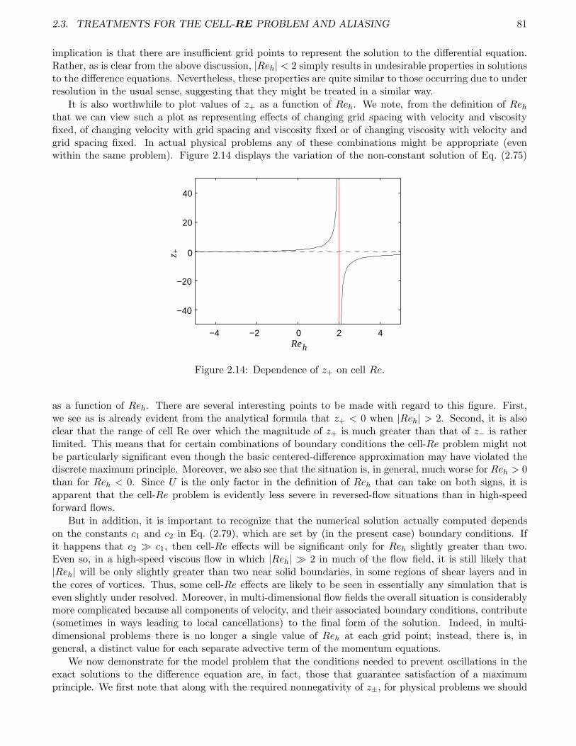
2.3. TREATMENTS FOR THE CELL-RE PROBLEM AND ALIASING 81
implication is that there are insufficient grid points to represent the solution to the differential equation.Rather, as is clear from the above discussion, |Reh| < 2 simply results in undesirable properties in solutionsto the difference equations. Nevertheless, these properties are quite similar to those occurring due to underresolution in the usual sense, suggesting that they might be treated in a similar way.
It is also worthwhile to plot values of z+ as a function of Reh. We note, from the definition of Rehthat we can view such a plot as representing effects of changing grid spacing with velocity and viscosityfixed, of changing velocity with grid spacing and viscosity fixed or of changing viscosity with velocity andgrid spacing fixed. In actual physical problems any of these combinations might be appropriate (evenwithin the same problem). Figure 2.14 displays the variation of the non-constant solution of Eq. (2.75)
-40
-20
0
20
40
-4 -2 0 2 4−4 −2 0 2 4
+z
−40
−20
0
20
40
Reh
Figure 2.14: Dependence of z+ on cell Re.
as a function of Reh. There are several interesting points to be made with regard to this figure. First,we see as is already evident from the analytical formula that z+ < 0 when |Reh| > 2. Second, it is alsoclear that the range of cell Re over which the magnitude of z+ is much greater than that of z− is ratherlimited. This means that for certain combinations of boundary conditions the cell-Re problem might notbe particularly significant even though the basic centered-difference approximation may have violated thediscrete maximum principle. Moreover, we also see that the situation is, in general, much worse for Reh > 0than for Reh < 0. Since U is the only factor in the definition of Reh that can take on both signs, it isapparent that the cell-Re problem is evidently less severe in reversed-flow situations than in high-speedforward flows.
But in addition, it is important to recognize that the numerical solution actually computed dependson the constants c1 and c2 in Eq. (2.79), which are set by (in the present case) boundary conditions. Ifit happens that c2 ≫ c1, then cell-Re effects will be significant only for Reh slightly greater than two.Even so, in a high-speed viscous flow in which |Reh| ≫ 2 in much of the flow field, it is still likely that|Reh| will be only slightly greater than two near solid boundaries, in some regions of shear layers and inthe cores of vortices. Thus, some cell-Re effects are likely to be seen in essentially any simulation that iseven slightly under resolved. Moreover, in multi-dimensional flow fields the overall situation is considerablymore complicated because all components of velocity, and their associated boundary conditions, contribute(sometimes in ways leading to local cancellations) to the final form of the solution. Indeed, in multi-dimensional problems there is no longer a single value of Reh at each grid point; instead, there is, ingeneral, a distinct value for each separate advective term of the momentum equations.
We now demonstrate for the model problem that the conditions needed to prevent oscillations in theexact solutions to the difference equation are, in fact, those that guarantee satisfaction of a maximumprinciple. We first note that along with the required nonnegativity of z±, for physical problems we should

82 CHAPTER 2. SPECIAL NUMERICAL DIFFICULTIES OF THE NAVIER–STOKES EQUATIONS
also require z± ∈ R. This latter requirement implies that in Eq. (2.77)
(a1
a2
)2
≥ 4
(a0
a2
),
or
|a1| ≥ 2√a0a2 . (2.81)
Now if we are to permit equality to hold in (2.81), the solution given by Eq. (2.77) can be positive onlyif
sgn(a1a2) = −1 . (2.82)
On the other hand, if strict inequality holds in (2.81), then we must require in addition to (2.82) that
a1
a2≥√(
a1
a2
)2
− 4
(a0
a2
).
But this can be guaranteed only if
sgn(a0a2) = +1 . (2.83)
We note that conditions (2.82) and (2.83), taken together, are equivalent to the usual non-negativityrequirement.
We will now show that satisfaction of the inequality (2.81) is equivalent to diagonal dominance. Againusing (2.82) and (2.83), we see that we can assume a0, a2 ≥ 0 and a1 < 0 hold. In this case, diagonaldominance would imply
|a1| ≥ |a0| + |a2| . (2.84)
Now since a0 and a2 are nonnegative, their square roots are real, and we have
(√a0 −
√a2)
2 ≥ 0 ⇒ a0 − 2√a0a2 + a2 ≥ 0 .
Thus,
2√a0a2 ≤ a0 + a2 = |a0| + |a2| . (2.85)
Now suppose diagonal dominance holds. Then
|a1| ≥ |a0| + |a2| ≥ 2√a0a2 ;
hence, inequality (2.81) is satisfied. On the other hand, suppose (2.81) does not hold; i.e.,
|a1| < 2√a0a2 .
Then, from inequality (2.85) it follows that diagonal dominance does not hold, completing the equivalenceproof.
Remedies for the Cell-Re Problem
In this subsection we will introduce several of the more widely-used treatments of the cell-Re problem.As we have hinted earlier, none of these provide a complete solution to the problem; moreover, fromdiscussions in the preceding section, it would appear likely that there cannot be a single approach thatis guaranteed to always work without causing other difficulties. The specific techniques we consider hereare first-order upwinding, the so-called “hybrid” scheme, second-order upwinding and QUICK. Nearly allcommercial CFD codes provide options for employing all of these except second-order upwinding (whichis available in some code, but not on others)—in addition to use of standard centered differencing, and insome codes even further options are available, thus underscoring the significance attached to this problem.
2.3. TREATMENTS FOR THE CELL-RE PROBLEM AND ALIASING 83
To understand why this is so, recall the basic centered approximation of the Burgers’ equation modelproblem, expressed here as
(1 +
Reh2
)ui−1 − 2ui +
(1 − Reh
2
)ui+1 = 0 . (2.86)
We again note that to prevent non-physical oscillatory solutions it is generally necessary to require
|Reh| ≤ 2 , (2.87)
which is termed the cell-Re restriction for centered-difference approximations. The consequence of thisrestriction is readily seen. Namely, suppose the flow velocity is O(1) and viscosity ν ∼ O(10−4), both ofwhich are reasonable magnitudes for physical problems. Now from inequality (2.87) it follows that the gridspacing h must satisfy
h ≤ 2ν
|U | . (2.88)
Hence, in the present case we have h ≤ 2×10⁻⁴, which in a 3-D calculation on the unit cube would requireover 1011 grid points. Clearly, this is a nearly intractable problem on current computing hardware, andit will probably not be routinely possible to achieve the industrial standard of “overnight turnaround” forproblems of this size any time in the next 10 years.
First-Order Upwinding. So-called first-order upwind differencing was probably the first proposed remedyfor the cell-Re problem. It was introduced on the basis of ad hoc “physical reasoning” (see, e.g., Patankar[40]). Namely, it was argued that the reason centered differencing led to non-physical solution oscilla-tions was that it could sense both upstream and downstream flow behavior, and it combined these in itsrepresentation of the velocity gradient. It was further argued that a difference approximation using onlyinformation carried in the flow direction would be more appropriate; i.e., the difference approximationsshould be one-sided (or at least biased) into the flow direction. The simplest such procedure is the basicfirst-order difference.
For the Burgers’ equation model problem with U > 0, this takes the form
UD−ui − νD20ui = 0 ,
or after expanding the difference operator symbolism, introducing the definition of cell Re and rearrangingthe results, (
1 +1
Reh
)ui−1 −
(1 +
2
Reh
)ui +
1
Rehui+1 = 0 . (2.89)
It is easily checked that this difference equation satisfies both the non-negativity and diagonal dominanceconditions needed to guarantee that no interior maxima or minima exist, independent of the value of Reh,and it is also easy to directly solve this difference equation, as we have already done for the centered-difference case. The result of this is that both independent roots of the characteristic equation analogousto Eq. (2.76) are nonnegative for any value of Reh > 0. This latter requirement is guaranteed to hold,in general, if we switch to a forward-difference approximation in cases where U < 0. It is left as anexercise for the reader to analyze this case; the results are essentially the same as those just given. Thus,we can summarize the first-order upwind discretization as follows, expressed here for non-constant U innon-conserved form:
Uiux|i =
UiD−ui , Ui > 0 ,
UiD+ui , Ui < 0 .(2.90)
There are at least two major difficulties with first-order upwind treatment of the cell-Re problem, andthese were recognized fairly soon after its introduction. The analysis of this that we present here followsthat of de Vahl Davis and Mallinson [50], who were among the first to analyze this approach in detail.
84 CHAPTER 2. SPECIAL NUMERICAL DIFFICULTIES OF THE NAVIER–STOKES EQUATIONS
It is clear that the simple first-order differences employed in Eq. (2.90) degrade the overall accuracyof a discretization in any case that second-, or higher-, order methods are being used for terms otherthan advective terms, and in conjunction with this is the fact that this reduction in accuracy is globalsince, presumably, we are usually solving boundary value problems. But there are additional, more subtle,problems that arise from first-order upwind differencing. To see this we consider the dimensionless form ofthe Burgers’ equation model problem,
Uux − 1
Reuxx = 0 , (2.91)
with U > 0. Equation (2.90) implies that upwind differencing will employ the backward difference
D−ui =ui − ui−1
h
in the advective term, and expansion of ui−1 yields the following:
ui−1 = ui − hux
∣∣i+h2
2uxx
∣∣i− h3
6uxxx
∣∣i± · · · .
This shows that Eq. (2.91) can be expressed as
Uux −(
1
Re+Uh
2
)uxx +
h2
6Uuxxx ± · · · = 0 ,
or
Uux − 1
Re∗uxx + O(h2) = 0 , (2.92)
where Re∗ is the effective Reynolds number defined as
Re∗ ≡ 1
1
Re+Uh
2
. (2.93)
Equation (2.92) is often termed the “modified equation,” and its significance is that it, rather thanthe original PDE, is solved to within second-order accuracy instead of first-order accuracy implied by thediscretization. This suggests that the numerical solution is a more accurate representation of solutionsto the modified equations than to solutions of the actual (in the case of the N.–S. equations, physical)equation(s). Thus, it is important to consider this modified equation in more detail.
What is rather obvious is that the only difference between physical and modified equations in the caseof first-order upwinding is the coefficient of the diffusion term. That is, in the modified equation theoriginal physical Reynolds number is replaced with the effective Reynolds number, Re∗ given in Eq. (2.93),and it is essential to understand the consequences of this. Indeed, it has often been argued that for veryhigh Re, the flow is convection dominated, and since upwinding imposes the “correct physics,” use of thisapproximation should be quite accurate. But this is a spurious argument, especially when simulating wall-bounded flows. In such flows, no matter what the value of Re, some regions of the flow will be significantlyaffected by viscous forces; consequently, if anything is done to the equations of motion to alter this aspectof the physics (the diffusion terms), it cannot be expected that accurate solutions will be obtained.
With this in mind, it is of interest to examine the specific effects of Re→ ∞ in the modified equation.In particular, consider the limit of Re∗ as Re→ ∞. It is easily seen from Eq. (2.93) that
limRe→∞
Re∗ =2
Uh. (2.94)
Hence, as the physical Reynolds number approaches infinity, the computational one approaches a finitelimit—in fact, one that could be quite small if coarse grids are employed. This provides an explanationfor a phenomenon observed in early uses of first-order upwinding; namely, it was seen that solutions for
2.3. TREATMENTS FOR THE CELL-RE PROBLEM AND ALIASING 85
a given physical situation and discrete approximation did not appear to change much with Re after thevalue of this parameter exceeded ∼ O(103). Of course, in most situations this is counter intuitive on aphysical basis, and it provided motivation for investigations of the sort we have just presented.
Clearly, the ultimate effect of first-order upwinding is to increase the coefficient of the diffusion term(s)in the governing equations. The factor producing this effect, Uh/2, (and similar factors arising in othermethods) is often called numerical diffusion or numerical viscosity. Although these factors are related to,and in many ways similar to, “artificial viscosity,” or “artificial dissipation,” in the present lectures we willconsider them to be distinct. In particular, numerical diffusion is, in general, an unwanted effect arising inan uncontrolled way from (usually) inadequate numerical analytic procedures—basically mistakes, whereasin essentially all cases artificial dissipation is added deliberately and at least to some extent, controllably, ina manner that has minimal effect on the physics represented by the final discrete equations. Furthermore,as is evident from (2.94), numerical diffusion can often completely dominate physical diffusion, and this isnot usually the case with artificial dissipation except when it is employed with inviscid forms (the Eulerequations) of the equations of motion.
The Hybrid Scheme. One of the early modifications that is still widely used today, especially as anoption in commercial CFD software, is the so-called “hybrid” scheme of Spalding [51] (also, see [40]). Inthis approach the solution is tested locally to determine whether a centered difference cell-Re restrictionviolation is likely, and if it is the scheme is automatically switched to first-order upwinding. To constructthis method for the model Burgers’ equation problem, we now consider the conservation form and allow Uto be the variable Ui, leading to
(Uu)x − νuxx = 0 . (2.95)
We first express the discrete equation in the general form valid for any 1-D three-point grid stencil,
a1ui−1 + a2ui + a3ui+1 = 0 ,
and then define the difference equation coefficients as follows:
a1 = max
[−Ui−1h, ν −
Ui−1h
2, 0
], (2.96a)
a2 = −a1 − a3 − h (Ui+1 − Ui−1) , (2.96b)
a3 = max
[Ui+1h, ν +
Ui+1h
2, 0
]. (2.96c)
It is important to recognize that if use of the hybrid method results in switching to first-order upwindingat very many grid points, the solution behavior will be no different than that of first-order upwinding itself,and this is often the case. Thus, we do not recommend its use. We have included it here simply for thesake of completeness; as we have already mentioned, it is widely used in commercial CFD codes.
In summarizing this presentation on first-order upwind differencing, we again emphasize that, while ituniformly cures the cell-Re problem, its use results in a possibly drastic alteration of the physics beingconsidered; the end result is that solutions obtained in this way cannot, in general, be trusted to accuratelyrepresent the physical phenomena being simulated. Thus, this approach should almost never be employed.But we note that there is one particular valid application for first-order upwind differencing. We will inChap. 3 present a detailed algorithm for solving the N.–S. equations in which δ-form quasilinearizationwill be used to treat nonlinearities appearing in the momentum equations. In this particular instance it isquite convenient, and effective, to utilize first-order upwinding in constructing the left-hand side Jacobianmatrix with respect to which the Newton iterations are computed. This is a valid approach provided theright-hand side of the equation is discretized in a physically-correct manner (i.e., different from first-orderupwinding) because approximate Jacobian matrices can be useful in Newton iteration procedures, and theone produced via first-order upwinding is numerically very stable.
86 CHAPTER 2. SPECIAL NUMERICAL DIFFICULTIES OF THE NAVIER–STOKES EQUATIONS
Second-Order Upwinding. Here we will very briefly treat an approach at one time favored by Shyy [52]and others, namely, use of second-order one-sided differences with switching similar to that employed infirst-order upwinding in order to difference into the flow direction. We again employ the conserved-formBurgers’ equation, (2.95), as our model problem. Then second-order upwinding takes the form
(Uu)x,i =1
2h
3Uiui − 4Ui−1ui−1 + Ui−2ui−2 , Ui > 0 ,
−Ui+2ui+2 + 4Ui+1ui+1 − 3Uiui , Ui < 0 .(2.97)
As is well known, this discretization is second-order accurate. Moreover, it turns out that the leadingterms of the modified equation are identical to those of the original equation. Thus, no physics has beencompromised by this approximation. It can also be checked (by setting U ≡ const. that the roots of thecorresponding difference equation are all nonnegative, independent of the value of cell Re. Hence, formally,there is no cell-Re restriction associated with this approximation. It should also be noted that neithernonnegativity of the difference equation coefficients nor diagonal dominance hold for this scheme, implyingthat it does not satisfy a maximum principle in the sense described earlier. The lesson to be taken from thisis that while satisfaction of these properties is desirable, it is not necessary in general, and more emphasisshould be placed on finding the solutions to the difference equation.
Finally, we observe that actual computational experience with second-order upwinding has been rathermixed. Shyy [52] claims it is the best of numerous methods that he tested. But other investigatorshave shown less favorable results. Furthermore, it is clear that Eq. (2.97) leads to a five-point discreterepresentation, resulting in a more complicated matrix structure if implicit time stepping is employedin the solution algorithm. Nevertheless, second-order upwinding is often an available option for treatingadvective terms of the N.–S. equations in commercial CFD codes.
QUICK. The quadratic upstream interpolation for convective kinematics scheme of Leonard [48] is oneof the most widely-used methods for treating the cell-Re problem. It is available as an option in mostcommercial CFD packages, and primarily for that reason we include it herein. The formula given belowcorresponds to the same Burgers’ equation model problem we have been considering throughout thesediscussions.
(Uu)x,i =1
8h
3Ui+1ui+1 + 3Uiui − 7Ui−1ui−1 + Ui−2ui−2 , Ui > 0 ,
−Ui+2ui+2 + 7Ui+1ui+1 − 3Uiui − 3Ui−1ui−1 , Ui < 0 .(2.98)
It is worthwhile to note that Leonard originally indicated third-order accuracy for this method, but thiswas with respect to a location in the grid stencil that did not correspond to any grid point. Careful analysisshows the scheme to be second-order accurate. This confusion likely still persists to the present; at leastsome commercial flow codes claim to have on option for third-order “upwinding,” and it is often a form ofQUICK that is being used. It is also useful to note that although this is a switching scheme like the twopreceding upwind methods, it is not truly an upwind approach, but rather an “upwind biased” scheme,because its stencil extends to both sides of the grid point in question.
As was true of the second-order upwind method, QUICK does not lead to nonnegativity of differenceequation coefficients, nor do corresponding coefficients exhibit diagonal dominance. But unlike the second-order upwinding procedure, QUICK does have a cell-Re restriction—and it is nearly as severe as that foundfor simple centered-difference approximations; viz.,
|Reh| ≤ 8/3 . (2.99)
Nevertheless, computational experience with QUICK has been generally favorable.There are numerous other upwind-like treatments of the cell-Re problem. Some have at times been fairly
widely used while most have been rather seldom employed. We do not intend to attempt an encyclopediccoverage of such methods, in large part because all have their shortcomings; and the ones discussed here

2.3. TREATMENTS FOR THE CELL-RE PROBLEM AND ALIASING 87
are most often used. It is worth mentioning, however, that a related treatment has received considerableattention in recent years, and it is usually quite successful. It is to employ techniques originally derivedfor use in shock capturing associated with solving the Euler equations of compressible flow. There areseveral classes of these methods, and we merely mention them here: flux-corrected transport (FCT), totalvariation diminishing (TVD) and essentially non-oscillatory (ENO). While use of such methods can behighly effective in terms of removing non-physical oscillations, they are in general somewhat more difficultto code, and they typically increase required arithmetic very significantly.
In closing this section we provide in Table 2.1 a summary of the methods for treating the cell-Reproblem that we have discussed in at least a cursory way. The table contains the independent roots of thedifference equation and the cell-Re restriction for the Burgers’ equation model problem, if any, for eachprocedure.
Table 2.1 Difference equation roots and cell-Re restrictions for model problem1 + jRehj ; 1(1+ 32 jRehj)q(1+ 32 jRehj)22jRehj2 ; 11+ 12Reh1 12Reh ; 1 jRehj 2(1+ 34 jRehj)q(1+ 34 jRehj)2 12 jRehj(1+ 38 jRehj)2(1+ 38 jRehj) ; 1 jRehj 8=3st
QUICK
nd
nd
RestrictionCell-ReScheme Roots of Difference Equation
1 -order upwind
2 -order upwind
2 -order centered
none
none
Use of absolute-value symbols in all of the formulas except that for centered differencing arises from thefact that all other techniques involve a switch in formulas so as to always be differencing in the (mainly)flow direction. As a consequence, there are actually two possible difference equations in each such case;but their roots are the same if one expresses them in terms of |Reh|.
2.3.2 Treatment of effects of aliasing
In this section we will first indicate in fairly precise detail just what “aliasing” is, and how it arises. Wewill see that its symptoms are somewhat similar to those of the cell-Re problem treated above, but itsroot cause is rather different. We will then consider techniques for treating this problem. It will be seenthat since aliasing arises from an inability of a numerical approximation to represent high-wavenumbercomponents in its solution, the remedy must always be some form of smoothing, or mollification, thatintroduces additional dissipation into the numerical scheme, and thus damps effects of high wavenumbers.
In the context of the N.–S. equations there have been three main approaches used to do this: i)flux modification, ii) artificial dissipation and iii) filtering. We mentioned the first two of these duringearlier discussion of the cell-Re problem; both have received considerable attention in the CFD literature,especially in the context of shock capturing in high-speed compressible flow simulations. Here, however, wewill emphasize the last possibility. This approach has been utilized mainly in the context of meteorologicalflows, but Yang and McDonough [53] and McDonough and Yang [54] have recently demonstrated itseffectiveness in simulations involving a Burgers’ equation model of turbulence. Moreover, applications ofthis approach to 2-D incompressible N.–S. flows have previously been presented by McDonough et al. [55]

88 CHAPTER 2. SPECIAL NUMERICAL DIFFICULTIES OF THE NAVIER–STOKES EQUATIONS
and [56], and to 3-D incompressible flows by McDonough and Yang [53]. Similar techniques are employedby Visbal and Gaitonde [58] and others.
How Aliasing Occurs
A straightforward, intuitive view of aliasing comes from the following simple plot, Fig. 2.15, in whichwe demonstrate an extreme case of under sampling of a signal. The basic signal is a sine function (plusits first subharmonic) with wavelength h, and it is being sampled at this same wavelength, presumably
sampled signal
actual signalh
0.0
Figure 2.15: Under-sampled oscillatory function demonstrating effects of aliasing.
for later reconstruction. It is evident that the sampled signal is a (nonzero) constant. Moreover, it canalso be seen that a Fourier analysis of the actual signal would show that its lowest mode (the average)has zero magnitude while the lowest (and only) mode of the sampled signal has magnitude near unity.We see from this that not only has the sampled signal lost the high-wavenumber content of the originalsignal, but it has also misrepresented even the lowest wavenumber, which in principle it should have beencapable of representing. Thus, what we term as aliasing has two main effects. It results in failure torepresent high-wavenumber (and/or high-frequency) behavior, and (as it turns out, a consequence of this)it incorrectly represents lower wavenumbers.
The mathematics associated with this has been known for a long time, especially in the context ofsignal processing. Here, we provide a description taken from the text by Ames [59]. Let f(x) be a functionin L2(−1, 1), and consider its Fourier representation given by
f(x) =∞∑
k=−∞
akeikπx (2.100)
with
ak =1
2
∫ 1
−1f(x)e−ikπx dx .
Now if one partitions the interval [−1, 1] with 2N uniformly-spaced points such that xj = j/N , for−N ≤ j < N , one can construct the (exact) Fourier polynomial which when evaluated at x = xj gives thevalue
fj =
N−1∑
m=−N
Ameimπj/N ,
where
Am =1
2N
N−1∑
j=−N
fje−imπj/N . (2.101)
2.3. TREATMENTS FOR THE CELL-RE PROBLEM AND ALIASING 89
The basic question at this point is, “How are the Ams, obtained from the discrete approximation, relatedto the actual Fourier coefficients, the aks?” To find this relationship we evaluate f(x) at the discrete pointx = xj = j/N :
f(xj) =∞∑
k=−∞
akeikπxj =
∞∑
k=−∞
akeikπj/N .
At this point we observe that due to periodicity of the complex exponential there can be only 2N distinctvalues of eikπj/N . Then for any finite N we can rewrite the infinite sum as
∞∑
k=−∞
akeikπj/N =
∞∑
k=−∞
N−1∑
n=−N
an+2Nkei(n+2Nk)πj/N . (2.102)
We now substitute the right-hand side of Eq. (2.102) for fj into Eq. (2.101) to obtain
Am =1
2N
N−1∑
j=−N
∞∑
k=−∞
N−1∑
n=−N
an+2Nkei(n+2Nk)πj/Ne−imπj/N
=∞∑
k=−∞
am+2Nk
= am +∑
|k|>0
am+2Nk , (2.103)
with the second equality following from discrete orthonormality of the complex exponentials.The first thing to notice regarding this result is that if it happens that only 2N Fourier coefficients of a
signal are nonzero, the coefficients of the Fourier polynomial will agree with these. Similarly, if the functionbeing represented by the Fourier series and Fourier polynomial is very smooth so that high-wavenumbercoefficients in the Fourier series go to zero rapidly as wavenumbers become large, the Fourier polynomialcoefficients will not differ greatly from the Fourier series coefficients. On the other hand, if the functionf is not very smooth so that high-wavenumber coefficients have significant magnitude, and at the sametime N is not sufficiently large, the difference between am and Am will be significant because am+2Nk willstill be large enough, even at very high values of k (and for all m, including m = 0), to contribute to thediscrepancy. This is the fundamental cause of aliasing.
At this point one might question what any of this has to do with the finite-difference/finite-volumeapproximations that are the main topic of these lectures. But the answer to this is quite straightforward.It is easily checked that the relationship between the discrete function values fj and the coefficients Am
of the Fourier polynomial in Eq. (2.101) is a linear transformation consisting of a 2N×2N matrix. Thatis, given any set of 2N function values we can construct the 2N Ams. Furthermore, the result of com-puting with a finite-difference or finite-volume method is a grid function consisting of a finite numberof values that is supposed to approximate, in some sense, the exact solution to the PDE that has beendiscretized. We also expect, based on discussions in Chap. 1, that this exact solution possesses a Fourierseries representation. Thus, our finite-difference approximation is, to within a linear transformation, aFourier polynomial intended to approximate the Fourier series of the exact solution. Hence, it is clear thatif there are insufficient grid points in the representation, the effect will be identical to under sampling ofa signal, and the result will be aliased. Conversely, a fully-resolved, fine-grid solution will not exhibit anyeffects of aliasing.
It is important to recognize that in the case of attempting to solve the N.–S. equations, this situationis exacerbated by nonlinearity capable of generating high-wavenumber modes—even when they are notpresent in initial data—in the time evolving solutions of these equations. This combination makes theproblem of aliasing very serious, especially for high-Re flows, and it is thus crucial to be able to treat iteffectively.

90 CHAPTER 2. SPECIAL NUMERICAL DIFFICULTIES OF THE NAVIER–STOKES EQUATIONS
Treatment of the Aliasing Problem
We have already mentioned the three main approaches currently employed to treat aliasing, and wehave also noted that independent of the details the end result must be an increase in dissipation inorder for a treatment to be effective. As noted earlier, flux-modification schemes can provide a suitableapproach despite the fact that they were originally designed to mitigate a rather different problem (Gibbsphenomenon oscillations in the presence of shocks), but one exhibiting similar symptoms. The same canbe said for use of artificial dissipation. The main difference between these approaches is in the details ofimplementation. Flux modification is specifically numerical (i.e., it is applied to the discrete equations),whereas introduction of artificial dissipation can be viewed also in an analytical context. Furthermore, flux-modification methods are relatively difficult to implement while addition of artificial dissipation terms isfairly straightforward, except possibly near boundaries. But it should also be mentioned that the end resultof flux modification is introduction of additional truncation error of a diffusive nature. Thus, in principle,given a flux-modification scheme it is possible to find an equivalent artificial dissipation, although this is notgenerally easy. Finally, we note (as we have already hinted) that considerable programming effort and/orextra floating-point arithmetic is involved with implementing either of these general classes of methods,especially the former.
In the current lectures we will present a different treatment of the aliasing problem. This approachis not new; indeed, it is actually older than flux-modification and cell-Re treatments (that sometimes aremistakenly attempted). It is use of post-processing filters as is routinely done in essentially all signalprocessing. (After all, a collection of numbers comprising a discrete solution can easily be interpreted asa “signal.”) Use of filters in the manner to be described here was probably first introduced by Shuman[25] and analyzed in considerable detail by Shapiro [60]—but not in the context of CFD. Our descriptionherein will be based on the modern treatment of PDEs given in Chap. 1 of these lectures.
We first recall the idea of a solution operator discussed in Chap. 1 and consider a discrete case of this.Recall that a solution operator is a mathematical construct that acts on initial data (prescribed at t = t0)to produce a solution at a later time t > t0. For example, if u0(x) provides initial data for some PDE andS is its solution operator, then we can formally express the solution at time t as
u(t) = S(t)u0 .
It is useful for our purposes here to associate S(t) with some form of (temporal) integration over the interval(t0, t], although this is not the only possible form (recall the solution operator for the heat equation, Eq.(1.17)).
We next observe that discrete solution operators can be easily constructed via formal numerical inte-gration of this form. Consider a nonlinear PDE with the representation
ut = N (u) ,
where N (u) represents some, generally, nonlinear (e.g., Navier–Stokes) spatial operator. We can integratethis to obtain
u(t) = u(t0) +
∫ t
t0
N (u) dτ ,
and replacing the integral on the right-hand side with a quadrature will yield a discrete solution operator.For example, if we were to use simple forward-Euler time integration, we would obtain
un+1 = un + kN (un) ,
and we can express this formally asun+1
h = Sh(k)unh (2.104)
to indicate that spatial discretization has been done with a grid of spacing h, and discrete time integrationis being performed with time step k.
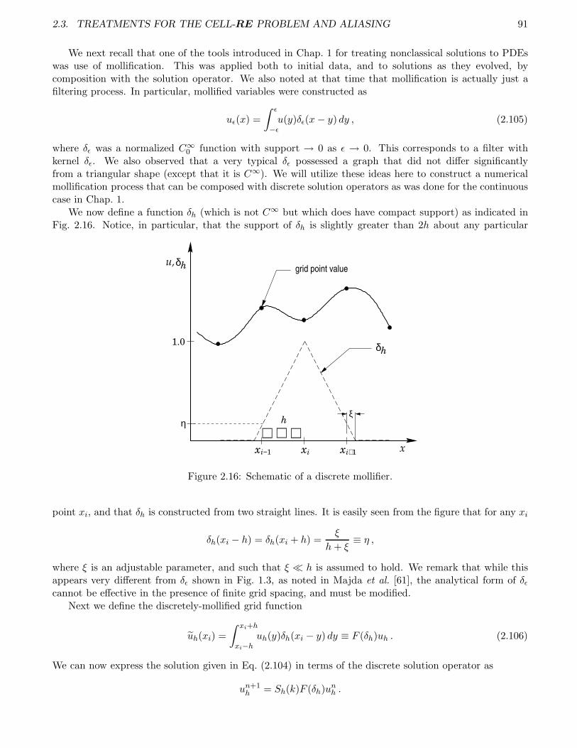
2.3. TREATMENTS FOR THE CELL-RE PROBLEM AND ALIASING 91
We next recall that one of the tools introduced in Chap. 1 for treating nonclassical solutions to PDEswas use of mollification. This was applied both to initial data, and to solutions as they evolved, bycomposition with the solution operator. We also noted at that time that mollification is actually just afiltering process. In particular, mollified variables were constructed as
uǫ(x) =
∫ ǫ
−ǫu(y)δǫ(x− y) dy , (2.105)
where δǫ was a normalized C∞0 function with support → 0 as ǫ → 0. This corresponds to a filter with
kernel δǫ. We also observed that a very typical δǫ possessed a graph that did not differ significantlyfrom a triangular shape (except that it is C∞). We will utilize these ideas here to construct a numericalmollification process that can be composed with discrete solution operators as was done for the continuouscase in Chap. 1.
We now define a function δh (which is not C∞ but which does have compact support) as indicated inFig. 2.16. Notice, in particular, that the support of δh is slightly greater than 2h about any particular
ξη h
xi−1 i+1xxi
grid point value
δh1.0
δhu,
x
Figure 2.16: Schematic of a discrete mollifier.
point xi, and that δh is constructed from two straight lines. It is easily seen from the figure that for any xi
δh(xi − h) = δh(xi + h) =ξ
h+ ξ≡ η ,
where ξ is an adjustable parameter, and such that ξ ≪ h is assumed to hold. We remark that while thisappears very different from δǫ shown in Fig. 1.3, as noted in Majda et al. [61], the analytical form of δǫcannot be effective in the presence of finite grid spacing, and must be modified.
Next we define the discretely-mollified grid function
uh(xi) =
∫ xi+h
xi−huh(y)δh(xi − y) dy ≡ F (δh)uh . (2.106)
We can now express the solution given in Eq. (2.104) in terms of the discrete solution operator as
un+1h = Sh(k)F (δh)un
h .

92 CHAPTER 2. SPECIAL NUMERICAL DIFFICULTIES OF THE NAVIER–STOKES EQUATIONS
We first observe that formally integration in (2.106) should be over the interval [xi − h− ξ, xi + h+ ξ],but there are no grid function values in the border regions of length ξ, so results (numerical) from theabove formula would be unchanged by including this. We now perform trapezoidal quadrature betweenxi − h and xi, and again between xi and xi + h. This results in
uh(xi) =h
2[2uh(xi)δh(xi − xi) + uh(xi−1)δh(xi − xi + h) + uh(xi+1)δh(xi − xi − h)]
=h
2[ηuh(xi−1) + 2uh(xi) + ηuh(xi+1)]
=ηh
2
[uh(xi−1) +
2
ηuh(xi) + uh(xi+1)
]. (2.107)
But for proper normalization of this discrete case we must require uh(xi) = uh(xi) if uh ≡ const. Thus, wemust have
uh(xi) =uh(xi−1) + βuh(xi) + uh(xi+1)
2 + β, (2.108)
with β ≡ 2/η. This is the filter used by Shuman [25], and we call β the filter parameter.It is clear that η → 0 as ξ → 0, and in this limit β → ∞. This has the same effect as ǫ → 0 in the
definition of mollifier given in Eq. (2.105) and would be equivalent if h → 0 also holds. Furthermore, itis clear from Eq. (2.106), the definition of the discrete mollifier, that uh(xi) → uh(xi) as h → 0. Whilethis is not immediately obvious from the final form of the Shuman filter given in Eq. (2.108), it can bedemonstrated via a simple truncation error analysis which we now carry out as follows.
We first express (2.108) in the more concise notation
ui =ui−1 + βui + ui+1
2 + β, (2.109)
and then expand ui−1 and ui+1 in Taylor series:
ui−1 = ui − hux|i +h2
2uxx|i −
h3
6uxxx|i ± · · · ,
and
ui+1 = ui + hux|i +h2
2uxx|i +
h3
6uxxx|i + · · · .
(We remark here that existence of derivatives needed to construct these expansions is, in general, opento question, especially for the N.–S. equations, and it may be necessary to view these in the sense ofdistributions, as discussed in Chap. 1.) Then substitution of these into the above yields
ui = ui +h2
2 + βuxx|i + O(h4) . (2.110)
This representation highlights two important features of this filter. First, it demonstrates that ui isbeing replaced with a quantity explicitly containing added dissipation—one of the main requirements forsuccessful treatment of aliasing. In particular, it can be seen that the dominant truncation error is diffusive,corresponding to addition of a scaled (discrete inthis case) Laplacian. At the same time, the actual amountof added diffusion is controllable through the parameter β and the grid spacing h. Thus, even though amodified equation would contain extra diffusion at the level of the (physical) second-order operators, thisgoes to zero with h2 rather than only as h in first-order upwinding. Moreover, it turns out that the O(h4)term is anti-diffusive, leading to some cancellation of the effects at second order.
There are several additional items that should be investigated for the filter given in Eq. (2.109). Thefirst of these is what is usually termed “frequency response” in the context of signal processing (in whichthe signals are typically functions of time), and which we will here more appropriately for our purposes
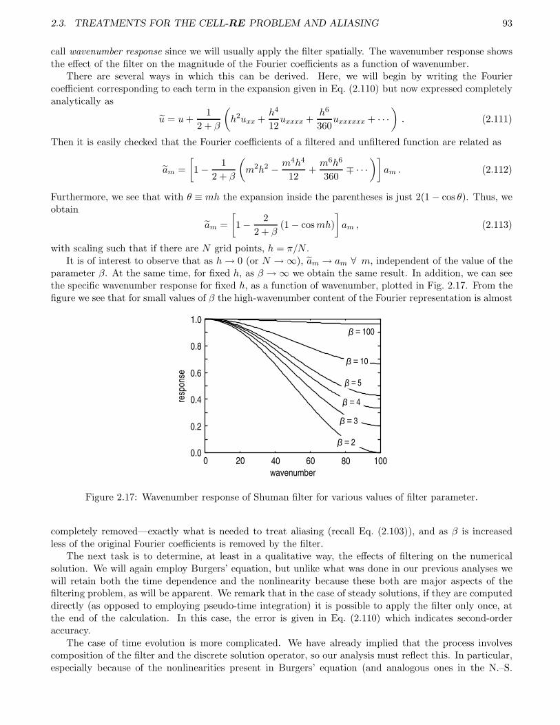
2.3. TREATMENTS FOR THE CELL-RE PROBLEM AND ALIASING 93
call wavenumber response since we will usually apply the filter spatially. The wavenumber response showsthe effect of the filter on the magnitude of the Fourier coefficients as a function of wavenumber.
There are several ways in which this can be derived. Here, we will begin by writing the Fouriercoefficient corresponding to each term in the expansion given in Eq. (2.110) but now expressed completelyanalytically as
u = u+1
2 + β
(h2uxx +
h4
12uxxxx +
h6
360uxxxxxx + · · ·
). (2.111)
Then it is easily checked that the Fourier coefficients of a filtered and unfiltered function are related as
am =
[1 − 1
2 + β
(m2h2 − m4h4
12+m6h6
360∓ · · ·
)]am . (2.112)
Furthermore, we see that with θ ≡ mh the expansion inside the parentheses is just 2(1 − cos θ). Thus, weobtain
am =
[1 − 2
2 + β(1 − cosmh)
]am , (2.113)
with scaling such that if there are N grid points, h = π/N .It is of interest to observe that as h→ 0 (or N → ∞), am → am ∀ m, independent of the value of the
parameter β. At the same time, for fixed h, as β → ∞ we obtain the same result. In addition, we can seethe specific wavenumber response for fixed h, as a function of wavenumber, plotted in Fig. 2.17. From thefigure we see that for small values of β the high-wavenumber content of the Fourier representation is almost
0
0.1
0.2
0.3
0.4
0.5
0.6
0.7
0.8
0.9
1
0 20 40 60 80 100
0 20 40 60 80 1000.0
0.2
0.4
0.6
0.8
1.0
wavenumber
resp
onse
β = 4
β = 2
β = 3
β = 5
β = 10
β = 100
Figure 2.17: Wavenumber response of Shuman filter for various values of filter parameter.
completely removed—exactly what is needed to treat aliasing (recall Eq. (2.103)), and as β is increasedless of the original Fourier coefficients is removed by the filter.
The next task is to determine, at least in a qualitative way, the effects of filtering on the numericalsolution. We will again employ Burgers’ equation, but unlike what was done in our previous analyses wewill retain both the time dependence and the nonlinearity because these both are major aspects of thefiltering problem, as will be apparent. We remark that in the case of steady solutions, if they are computeddirectly (as opposed to employing pseudo-time integration) it is possible to apply the filter only once, atthe end of the calculation. In this case, the error is given in Eq. (2.110) which indicates second-orderaccuracy.
The case of time evolution is more complicated. We have already implied that the process involvescomposition of the filter and the discrete solution operator, so our analysis must reflect this. In particular,especially because of the nonlinearities present in Burgers’ equation (and analogous ones in the N.–S.
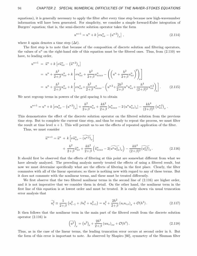
94 CHAPTER 2. SPECIAL NUMERICAL DIFFICULTIES OF THE NAVIER–STOKES EQUATIONS
equations), it is generally necessary to apply the filter after every time step because new high-wavenumberinformation will have been generated. For simplicity, we consider a simple forward-Euler integration ofBurgers’ equation; that is, the semi-discrete solution operator takes the form
un+1 = un + k[νun
xx −(un 2
)x
], (2.114)
where k again denotes a time step (∆t).The first step is to note that because of the composition of discrete solution and filtering operators,
the values of un on the right-hand side of this equation must be the filtered ones. Thus, from (2.110) wehave, to leading order,
un+1 = un + k[νun
xx −(un 2
)x
]
= un +h2
2+βun
xx + k
[νun
xx +h2
2+βun
xxxx −((
un +h2
2+βun
xx
)2)
x
]
= un +h2
2+βun
xx + k
[νun
xx+h2
2+βun
xxxx−(un 2+
2h2
2+βunun
xx+h4
(2+β)2un 2
xx
)
x
]. (2.115)
We next regroup terms in powers of the grid spacing h to obtain
un+1 = un + k[νun
xx −(un 2
)x
]+
h2
2+βun
xx +kh2
2+β[un
xxxx − 2 (ununxx)x] − kh4
(2+β)2(un 2
xx
)x.
This demonstrates the effect of the discrete solution operator on the filtered solution from the previoustime step. But to complete the current time step, and thus be ready to repeat the process, we must filterthe result at time level n+ 1. This will permit us to see the effects of repeated application of the filter.
Thus, we must consider
un+1 = un + k[νun
xx − (un 2)x
]
+h2
2+βun
xx +kh2
2+β
(un
xxxx − 2 ˜(ununxx)x
)− kh4
(2+β)2(un 2
xx )x . (2.116)
It should first be observed that the effects of filtering at this point are somewhat different from what wehave already analyzed. The preceding analysis merely treated the effects of using a filtered result, butnow we must determine specifically what are the effects of filtering in the first place. Clearly, the filtercommutes with all of the linear operators; so there is nothing new with regard to any of these terms. Butit does not commute with the nonlinear terms, and these must be treated differently.
We first observe that the two filtered nonlinear terms in the second line of (2.116) are higher order,and it is not imperative that we consider them in detail. On the other hand, the nonlinear term in thefirst line of this equation is at lowest order and must be treated. It is easily shown via usual truncationerror analysis that
u2i ≡ 1
2+β
(u2
i−1 + βu2i + u2
i+1
)= u2
i +2h2
2+β(uiui,x)x + O(h4) . (2.117)
It then follows that the nonlinear term in the main part of the filtered result from the discrete solutionoperator (2.116) is (
u2)x
=(u2)x
+2h2
2+β(uux)xx + O(h4) . (2.118)
Thus, as in the case of the linear terms, the leading truncation error occurs at second order in h. Butthe form of this error is important to note. As observed by Shapiro [60], symmetry of the Shuman filter
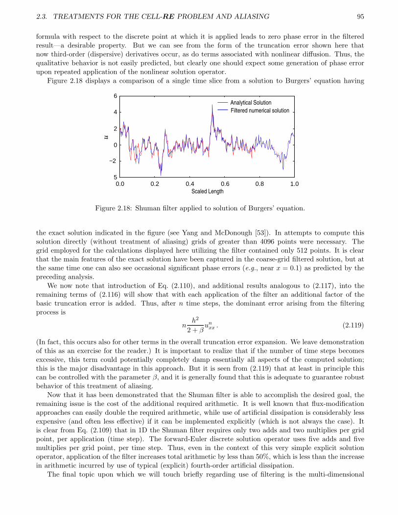
2.3. TREATMENTS FOR THE CELL-RE PROBLEM AND ALIASING 95
formula with respect to the discrete point at which it is applied leads to zero phase error in the filteredresult—a desirable property. But we can see from the form of the truncation error shown here thatnow third-order (dispersive) derivatives occur, as do terms associated with nonlinear diffusion. Thus, thequalitative behavior is not easily predicted, but clearly one should expect some generation of phase errorupon repeated application of the nonlinear solution operator.
Figure 2.18 displays a comparison of a single time slice from a solution to Burgers’ equation having
Scaled Length
u
0.8 1 1.2 1.4 1.6 1.8
0.0 0.2 0.4 0.6 0.8 1.00.8 1 1.2 1.4 1.6 1.80.8 1 1.2 1.4 1.6 1.8
Analytical Solution
Filtered numerical solution
-3
5
6
0
-3
-2
0
1
3
4
5
−2
2
4
Figure 2.18: Shuman filter applied to solution of Burgers’ equation.
the exact solution indicated in the figure (see Yang and McDonough [53]). In attempts to compute thissolution directly (without treatment of aliasing) grids of greater than 4096 points were necessary. Thegrid employed for the calculations displayed here utilizing the filter contained only 512 points. It is clearthat the main features of the exact solution have been captured in the coarse-grid filtered solution, but atthe same time one can also see occasional significant phase errors (e.g., near x = 0.1) as predicted by thepreceding analysis.
We now note that introduction of Eq. (2.110), and additional results analogous to (2.117), into theremaining terms of (2.116) will show that with each application of the filter an additional factor of thebasic truncation error is added. Thus, after n time steps, the dominant error arising from the filteringprocess is
nh2
2 + βun
xx . (2.119)
(In fact, this occurs also for other terms in the overall truncation error expansion. We leave demonstrationof this as an exercise for the reader.) It is important to realize that if the number of time steps becomesexcessive, this term could potentially completely damp essentially all aspects of the computed solution;this is the major disadvantage in this approach. But it is seen from (2.119) that at least in principle thiscan be controlled with the parameter β, and it is generally found that this is adequate to guarantee robustbehavior of this treatment of aliasing.
Now that it has been demonstrated that the Shuman filter is able to accomplish the desired goal, theremaining issue is the cost of the additional required arithmetic. It is well known that flux-modificationapproaches can easily double the required arithmetic, while use of artificial dissipation is considerably lessexpensive (and often less effective) if it can be implemented explicitly (which is not always the case). Itis clear from Eq. (2.109) that in 1D the Shuman filter requires only two adds and two multiplies per gridpoint, per application (time step). The forward-Euler discrete solution operator uses five adds and fivemultiplies per grid point, per time step. Thus, even in the context of this very simple explicit solutionoperator, application of the filter increases total arithmetic by less than 50%, which is less than the increasein arithmetic incurred by use of typical (explicit) fourth-order artificial dissipation.
The final topic upon which we will touch briefly regarding use of filtering is the multi-dimensional
96 CHAPTER 2. SPECIAL NUMERICAL DIFFICULTIES OF THE NAVIER–STOKES EQUATIONS
case. All of our analyses have been one-dimensional, but we note that there is a formal, although ad hoc,extension to multi-dimensions, which in 2D is
ui,j =ui−1,j + ui,j−1 + βui,j + ui,j+1 + ui+1,j
4 + β. (2.120)
Moreover, an extension of this form to 3D is obvious. We note that all of the preceding development relieson uniform grid spacing in Cartesian coordinates. Little beyond preliminary studies has been completedfor more complicated problem domains and non-uniform gridding. Moreover, a rigorous extension ofthe Shuman filter to higher dimensions is likely to result in a more complex grid stencil than the onecorresponding to (2.120).
2.4 Summary
In this chapter we have presented a number of somewhat special aspects of the incompressible Navier–Stokesequations that require more than just a basic knowledge of numerical analysis to successfully treat them.We began the chapter by discussing the various forms of the N.–S. equations that have been employedthrough the years in efforts to mitigate some of the difficulties that arise in numerical simulations. Weobserved that of these only the stream function/vorticity and primitive-variable formulations have seenwide application. But in modern 3-D simulations the latter of these is essentially the only viable approachbecause the former has no direct extension from 2D to 3D. The primitive-variable form, itself, has numerousdistinct subforms, all of which are analytically equivalent but which produce different behaviors in numericalimplementations.
Following the discussions of N.–S. equation forms we considered the problem of pressure-velocity cou-pling. We began with fairly detailed descriptions of the three main types of grid structures that have beenemployed in efforts to achieve this coupling; these are: i) (natural) unstaggered, ii) partially staggeredand iii) (fully) staggered. There is also an important modification of the unstaggered grid, often termednonstaggered, or more appropriately, co-located. It was noted that there is a very fundamental mathe-matical constraint, known as the div-stability condition, which imposes restrictions on the combinationof grid structure and form of discretization of the governing equations that must be used to guaranteethat discretely divergence-free velocity fields converge to continuous divergence-free ones as grid spacingis refined. These restrictions are automatically satisfied by centered discretizations on a staggered grid,and with modifications to the discretization of either the advective terms of the momentum equations ortreatment of the pressure Poisson equation, or both, they can be satisfied on co-located (cell-centered,unstaggered) grids. We observed that failure to satisfy the div-stability condition can lead to so-called“checkerboard” solutions containing non-physical, and yet very stable, oscillatory behaviors. The naturalunstaggered and partially staggered grid configurations are prone to producing such behaviors.
The final topics treated in this chapter, like checkerboarding, are associated with the tendency ofdiscrete solutions to the N.–S. equations to exhibit physically unrealistic oscillations. These can arise fromeither (or both) of two forms of under resolution, and their treatment has constituted a significant portionof the archival literature of CFD. The first of these, termed the cell-Re problem, is very specifically aproperty of the difference approximations employed to treat the combination of advection and diffusionterms, as appear in any transport equation—even linear ones. In this linear case it is possible to exactlysolve the corresponding difference equations, thus permitting detailed analysis of the cell-Re problem andits origins. We presented such analyses above, and we discussed several proposed remedies. But it must beemphasized that the most important consequence of these analyses is that there is no single modificationto the discrete equations that is guaranteed to always be effective for all flow conditions, or sometimes evenat all locations of a flow under fixed conditions.
The second topic covered in the last section of this chapter was that of aliasing. We described the basicnature of aliasing—what it is, and how it arises—and provided a specific representation of its effects interms of a Fourier expansion. We noted that the basic problem arises when discretization step sizes are

2.4. SUMMARY 97
too large to permit resolution of high-wavenumber components of the true solution. It can be expectedfrom the form of the Fourier representation that the observed consequence of aliasing will be spuriousoscillations in a computed solution—the same symptom as seen in the cell-Re problem. It is well knownin the field of signal processing that the universal treatment of aliasing is application of a filter to thealiased signal. (Of course, the filter needed for this is not universal, and depends strongly on the type ofsignal being treated.) Moreover, we saw in Chap. 1 that the analytical treatment of non-smooth solutions(those having significant high-wavenumber content) to PDEs was use of a mollifier, which is in fact a filter.Thus, in the present chapter we derived a discrete form of the typical analytical mollification operator andfound that this was precisely the Shuman filter [25]. We then showed in a formal way how this can beapplied to treat both cell-Re and aliasing problems. In particular, it was shown how to construct a formaldiscrete solution operator that employs the filter to smooth the solution at the end of each time step (postprocessing) before starting the next time step.

98 CHAPTER 2. SPECIAL NUMERICAL DIFFICULTIES OF THE NAVIER–STOKES EQUATIONS
Chapter 3
Solution Algorithms for the N.–S. Equations
In this chapter we will present many of the main solution algorithms that have been developed and usedthrough the years in efforts to solve the incompressible Navier–Stokes equations. We will do this by meansof a more or less chronological ordering to provide a sense of how the current understanding of solutionmethods has evolved. For each method treated we will usually provide a fairly complete derivation alongwith details of implementation, and in most cases a detailed pseudo-language algorithm.
Thus, in the first section we will derive and discuss the marker-and-cell (MAC) method of Harlow andWelch [36]. We follow this with a presentation of the SOLA method. At this point, it turns out that atleast two methods were introduced nearly simultaneously: these are artificial compressibility and projectionmethods. We will treat these in this order because there is a fairly direct relationship between artificialcompressibility and SOLA, and also between projection methods and the SIMPLE algorithms that will bethe last to be discussed, but are at present the most widely used—especially in commercial CFD software.
Before beginning these treatments we again present the Navier–Stokes equations in the form that theywill most often be encountered in the remainder of these lectures; namely
ut + (u2)x + (u v)y = −px + ν∆u , (3.1a)
vt + (u v)x + (v2)y = −py + ν∆v , (3.1b)
andux + vy = 0 . (3.2)
We observe that the algorithms to be presented in the sequel are of two main types. MAC, SIMPLE andthe projection methods employ a pressure Poisson equation to satisfy the divergence-free constraint, Eq.(3.2), while SOLA and the artificial compressibility method attempt to satisfy this condition by directlysolving modifications of (3.2). Both approaches have been fairly successful; the latter is widely used in thecontext of finite-element implementations. On the other hand, essentially all commercial CFD softwaremakes use of the former approach. In what follows we will have the opportunity to compare these twoclasses of techniques.
3.1 The Marker-and-Cell Method
The marker-and-cell technique was first proposed by Harlow and Welch [36] as a method for solvingfree-surface problems, but the staggered arrangement of dependent variables proved to be so effective atpreventing checkerboard solutions (because it automatically satisfies the div-stability condition) that it hasbecome an important method in its own right. Here, we will put little emphasis on the free-surface aspectsof its implementation. We begin with formal discretization of the momentum equations, followed by moredetailed treatment of the PPE. We then discuss implementation of boundary conditions for this latterequation and briefly describe computation of marker trajectories. We then conclude with a coarse-grainedpseudo-language algorithm suitable for MAC implementation.
99
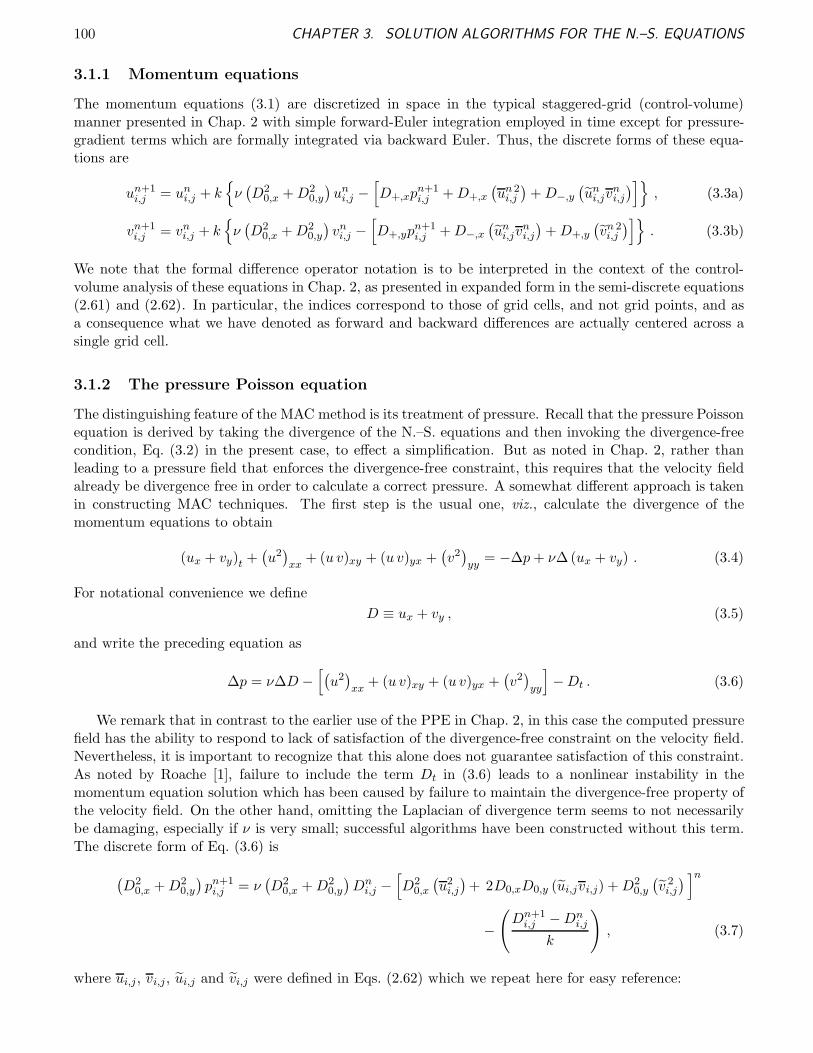
100 CHAPTER 3. SOLUTION ALGORITHMS FOR THE N.–S. EQUATIONS
3.1.1 Momentum equations
The momentum equations (3.1) are discretized in space in the typical staggered-grid (control-volume)manner presented in Chap. 2 with simple forward-Euler integration employed in time except for pressure-gradient terms which are formally integrated via backward Euler. Thus, the discrete forms of these equa-tions are
un+1i,j = un
i,j + kν(D2
0,x +D20,y
)un
i,j −[D+,xp
n+1i,j +D+,x
(un 2
i,j
)+D−,y
(un
i,jvni,j
)], (3.3a)
vn+1i,j = vn
i,j + kν(D2
0,x +D20,y
)vni,j −
[D+,yp
n+1i,j +D−,x
(un
i,jvni,j
)+D+,y
(vn 2i,j
)]. (3.3b)
We note that the formal difference operator notation is to be interpreted in the context of the control-volume analysis of these equations in Chap. 2, as presented in expanded form in the semi-discrete equations(2.61) and (2.62). In particular, the indices correspond to those of grid cells, and not grid points, and asa consequence what we have denoted as forward and backward differences are actually centered across asingle grid cell.
3.1.2 The pressure Poisson equation
The distinguishing feature of the MAC method is its treatment of pressure. Recall that the pressure Poissonequation is derived by taking the divergence of the N.–S. equations and then invoking the divergence-freecondition, Eq. (3.2) in the present case, to effect a simplification. But as noted in Chap. 2, rather thanleading to a pressure field that enforces the divergence-free constraint, this requires that the velocity fieldalready be divergence free in order to calculate a correct pressure. A somewhat different approach is takenin constructing MAC techniques. The first step is the usual one, viz., calculate the divergence of themomentum equations to obtain
(ux + vy)t +(u2)xx
+ (u v)xy + (u v)yx +(v2)yy
= −∆p+ ν∆ (ux + vy) . (3.4)
For notational convenience we define
D ≡ ux + vy , (3.5)
and write the preceding equation as
∆p = ν∆D −[(u2)xx
+ (u v)xy + (u v)yx +(v2)yy
]−Dt . (3.6)
We remark that in contrast to the earlier use of the PPE in Chap. 2, in this case the computed pressurefield has the ability to respond to lack of satisfaction of the divergence-free constraint on the velocity field.Nevertheless, it is important to recognize that this alone does not guarantee satisfaction of this constraint.As noted by Roache [1], failure to include the term Dt in (3.6) leads to a nonlinear instability in themomentum equation solution which has been caused by failure to maintain the divergence-free property ofthe velocity field. On the other hand, omitting the Laplacian of divergence term seems to not necessarilybe damaging, especially if ν is very small; successful algorithms have been constructed without this term.The discrete form of Eq. (3.6) is
(D2
0,x +D20,y
)pn+1
i,j = ν(D2
0,x +D20,y
)Dn
i,j −[D2
0,x
(u2
i,j
)+ 2D0,xD0,y (ui,jvi,j) +D2
0,y
(v 2i,j
) ]n
−(Dn+1
i,j −Dni,j
k
), (3.7)
where ui,j, vi,j, ui,j and vi,j were defined in Eqs. (2.62) which we repeat here for easy reference:
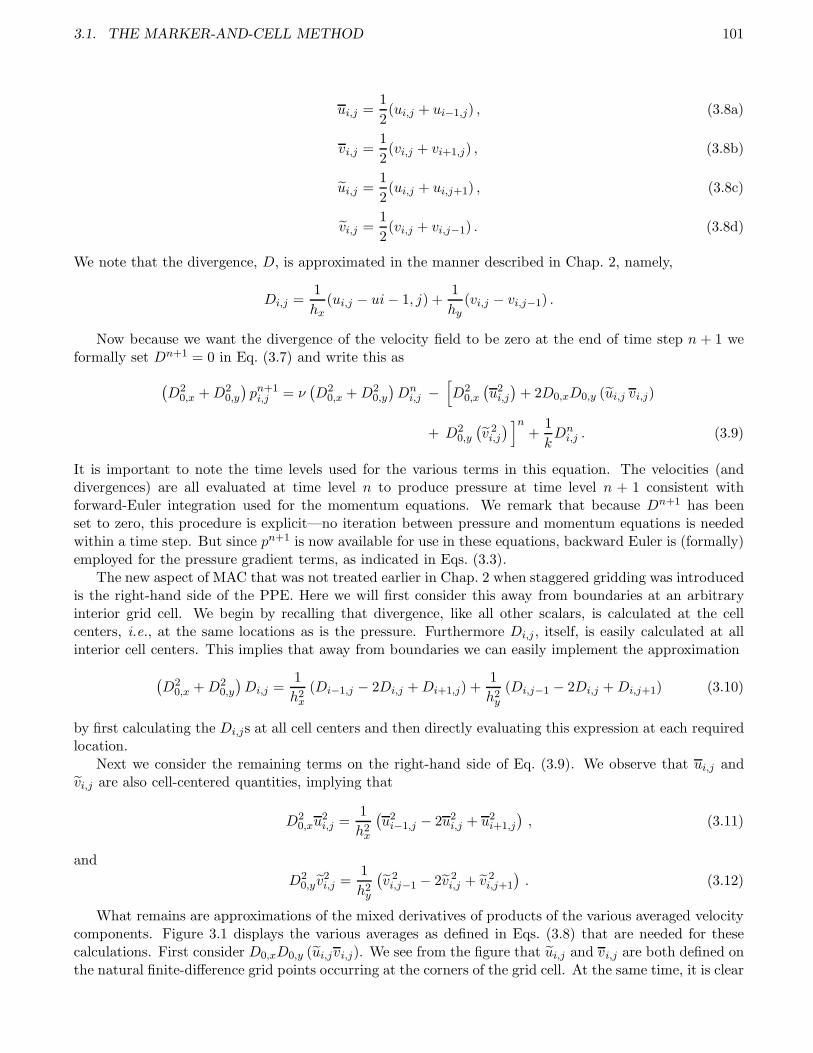
3.1. THE MARKER-AND-CELL METHOD 101
ui,j =1
2(ui,j + ui−1,j) , (3.8a)
vi,j =1
2(vi,j + vi+1,j) , (3.8b)
ui,j =1
2(ui,j + ui,j+1) , (3.8c)
vi,j =1
2(vi,j + vi,j−1) . (3.8d)
We note that the divergence, D, is approximated in the manner described in Chap. 2, namely,
Di,j =1
hx(ui,j − ui− 1, j) +
1
hy(vi,j − vi,j−1) .
Now because we want the divergence of the velocity field to be zero at the end of time step n + 1 weformally set Dn+1 = 0 in Eq. (3.7) and write this as
(D2
0,x +D20,y
)pn+1
i,j = ν(D2
0,x +D20,y
)Dn
i,j −[D2
0,x
(u2
i,j
)+ 2D0,xD0,y (ui,j vi,j)
+ D20,y
(v 2i,j
) ]n+
1
kDn
i,j . (3.9)
It is important to note the time levels used for the various terms in this equation. The velocities (anddivergences) are all evaluated at time level n to produce pressure at time level n + 1 consistent withforward-Euler integration used for the momentum equations. We remark that because Dn+1 has beenset to zero, this procedure is explicit—no iteration between pressure and momentum equations is neededwithin a time step. But since pn+1 is now available for use in these equations, backward Euler is (formally)employed for the pressure gradient terms, as indicated in Eqs. (3.3).
The new aspect of MAC that was not treated earlier in Chap. 2 when staggered gridding was introducedis the right-hand side of the PPE. Here we will first consider this away from boundaries at an arbitraryinterior grid cell. We begin by recalling that divergence, like all other scalars, is calculated at the cellcenters, i.e., at the same locations as is the pressure. Furthermore Di,j , itself, is easily calculated at allinterior cell centers. This implies that away from boundaries we can easily implement the approximation
(D2
0,x +D20,y
)Di,j =
1
h2x
(Di−1,j − 2Di,j +Di+1,j) +1
h2y
(Di,j−1 − 2Di,j +Di,j+1) (3.10)
by first calculating the Di,js at all cell centers and then directly evaluating this expression at each requiredlocation.
Next we consider the remaining terms on the right-hand side of Eq. (3.9). We observe that ui,j andvi,j are also cell-centered quantities, implying that
D20,xu
2i,j =
1
h2x
(u2
i−1,j − 2u2i,j + u2
i+1,j
), (3.11)
and
D20,y v
2i,j =
1
h2y
(v 2i,j−1 − 2v 2
i,j + v 2i,j+1
). (3.12)
What remains are approximations of the mixed derivatives of products of the various averaged velocitycomponents. Figure 3.1 displays the various averages as defined in Eqs. (3.8) that are needed for thesecalculations. First consider D0,xD0,y (ui,jvi,j). We see from the figure that ui,j and vi,j are both defined onthe natural finite-difference grid points occurring at the corners of the grid cell. At the same time, it is clear
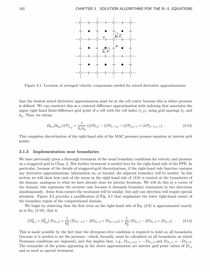
102 CHAPTER 3. SOLUTION ALGORITHMS FOR THE N.–S. EQUATIONS
u, v_ ∼
u, v_∼
u
v
Figure 3.1: Location of averaged velocity components needed for mixed derivative approximations.
that the desired mixed derivative approximation must be at the cell center because this is where pressureis defined. We can construct this as a centered difference approximation with indexing that associates theupper right-hand finite-difference grid point of a cell with the cell index (i, j), using grid spacings hx andhy. Thus, we obtain
D0,xD0,y (u v)i,j =1
hxhy((u v)i,j − (u v)i−1,j − (u v)i,j−1 + (u v)i−1,j−1) . (3.13)
This completes discretization of the right-hand side of the MAC pressure poisson equation at interior gridpoints.
3.1.3 Implementation near boundaries
We have previously given a thorough treatment of the usual boundary conditions for velocity and pressureon a staggered grid in Chap. 2. But further treatment is needed here for the right-hand side of the PPE. Inparticular, because of the details of staggered-grid discretizations, if the right-hand side function containsany derivative approximations, information on, or beyond, the adjacent boundary will be needed. In thissection we will show how each of the terms in the right-hand side of (3.9) is treated at the boundaries ofthe domain, analogous to what we have already done for interior locations. We will do this at a corner ofthe domain; this represents the severest case because it demands boundary treatments in two directionssimultaneously. Away from corners the treatment will be similar, but only one direction will require specialattention. Figure 3.2 provides a modification of Fig. 3.1 that emphasizes the lower right-hand corner ofthe boundary region of the computational domain.
We begin by observing that the first term on the right-hand side of Eq. (3.9) is approximated exactlyas in Eq. (3.10); that is
(D2
0,x +D20,y
)DNx,2 =
1
h2x
(DNx−1,2 − 2DNx,2 +DNx+1,2) +1
h2y
(DNx,1 − 2DNx,2 +DNx,3) . (3.14)
This is made possible by the fact that the divergence-free condition is required to hold on all boundaries(because it is needed to set the pressure—which, formally, must be calculated on all boundaries on whichNeumann conditions are imposed), and this implies that, e.g., DNx+1,2 = −DNx,2 and DNx,1 = −DNx,2.The remainder of the points appearing in the above approximation are interior grid point values of Di,j
and so need no special treatment.
3.1. THE MARKER-AND-CELL METHOD 103
u, v_∼
N x( ,2 )
u, v_ ∼
bottomboundary
boundaryright
u
v
Figure 3.2: Near-boundary grid cells for treatment of right-hand side of Eq. (3.9).
Next we consider Eq. (3.11) evaluated at the point (Nx, 2). This now takes the form
D20,xu
2Nx,2 =
1
h2x
(u2
Nx−1,2 − 2u2Nx,2 + u2
Nx+1,2
),
where only the term u2Nx+1,2 needs any special attention. But this value occurs at the cell center in the
image cell to the right of the interior point (Nx, 2). The u-component of velocity on the vertical boundaryof this cell must satisfy a zero mass flux condition because of the solid wall. As a consequence, we must haveu2
Nx+1,2 = −u2Nx,2, and this completes evaluation of this approximation. The approximation of D2
0,y v2i,j
corresponding to Eq. (3.12) is done in a completely analogous way, using the same reasoning.Similarly, approximation of the first mixed-derivative term, D0,xD0,y (u v)i,j, given in Eq. (3.13), is
completely trivial. Three of its four entries on the right-hand side are products of velocity componentsresiding on physical (solid) boundaries, and the remaining entry is an interior point. Hence, no specialtreatment is needed.
3.1.4 Marker particle trajectories for free surface tracking
The final item we treat with regard to the MAC method is its ability to predict the location of free surfaces.This is accomplished by introducing massless marker particles in the flow and following their Lagrangiantrajectories as the flow field evolves in time. Figure 3.3 provides an indication of how this is done inpractice. In particular, at the time marker particles are first introduced it is common to place four orfive markers in each grid cell, as noted in [1]. Because these are massless, they follow the velocity field toproduce Lagrangian pathlines, and this is implemented by noting that the (x, y) position of a particle isgiven by
dxp
dt= u ,
dyp
dt= v , (3.15)
or
xn+1p = xn
p +
∫ tn+1
tnu dt , (3.16a)
yn+1p = yn
p +
∫ tn+1
tnv dt . (3.16b)

104 CHAPTER 3. SOLUTION ALGORITHMS FOR THE N.–S. EQUATIONS
marker particles
Figure 3.3: Introduction of massless marker particles.
Forward-Euler integration, e.g., then leads to
xn+1p = xn
p + kup , (3.17a)
yn+1p = yn
p + kvp , (3.17b)
where up and vp represent appropriately interpolated velocity components at the location (xp, yp), asdiscussed next, and k is the time step used to integrate the momentum equations.
Clearly, there are two main problems associated with this approach. The first is interpolation of thevelocity field at each time step to provide computed results at correct Lagrangian locations so that thenumerical integration can be conducted. It has been typical to employ multi-linear interpolation, butobviously for complicated flow behavior this would prove to be rather inaccurate except on very fine grids.Thus, higher-order methods might be desirable, including use of cubic splines. It should also be notedthat on highly non-orthogonal generalized-coordinate grids it may be necessary to employ contravariantvelocity components
The second problem is the numerical integration itself. Here, we have employed simple forward-Eulerintegration as was done in the original presentation of the MAC method in [36]. This is consistent withthe order of accuracy of the velocity field simulation. But, especially if a higher-order integration scheme isused to solve the momentum equations, as will be done later for other techniques (and could be done here,as well), then it would be desirable to employ more accurate integrations to obtain the particle trajectories.Another approach is to use multiple time steps of smaller size than the momentum equation time steps toproduce smoother particle trajectories.
It should be clear that the initial placement of marker particles indicated in Fig. 3.3 is rather arbitrary,as is the number of particles per grid cell. Handling details such as these is generally left to the specificimplementation. A related problem is introduction of new particles at later times in situations that resultin some (or even all) of the original particles exiting the computational domain. There are numerous casesto be dealt with in this regard, and methods of treatment tend to be ad hoc. Thus, we will not providefurther discussions here.
Finally, we mention that despite the fact that the MAC method is intended for treating free surfaces,no effects of surface tension have been incorporated in this basic formulation. Correspondingly, no specificeffort is made to guarantee satisfaction of free-surface kinematic conditions. Despite all this, MAC has beena quite successful tool, both for simulating free-surface flows, and for incompressible flow in general—andit was the first method to have this capability. Nevertheless, there are by now more modern (and better)
3.2. SOLA METHOD 105
approaches, and we will discuss these in the sequel. Before doing that, however, we will end this sectionwith a presentation of the formal MAC algorithm and some closing discussions associated with it.
3.1.5 The MAC algorithm
In this final subsection we present a coarse-grained pseudo-language algorithm that summarizes the essentialparts of the MAC approach.
Algorithm 3.1 (Marker and Cell) Suppose n time steps have been completed. To advance the solution totime level n+ 1, perform the following steps:
1. load right-hand side of discrete PPE (3.9) using time level n velocity results to calculate divergencesand other terms;
2. solve the PPE for time level n+ 1 pressure using any appropriate elliptic solver;
3. apply explicit Euler integration to advance the momentum equations to time level n + 1 using timelevel n information for all terms except those corresponding to pressure gradients;
4. if marker particles are active, perform required interpolations and ODE integrations of Eqs. (3.16) toadvance particle locations to the n+ 1 time level.
It should be noticed that because forward-Euler (explicit) integration is used in the momentum equa-tions, the time stepping is only conditionally stable. In particular, if Re is small, we expect the time stepto be limited by diffusive stability requirements similar to those needed for the heat equation. On theother hand, if Re is relatively large we would expect that a CFL-type condition would be required. Resultspresented in Fletcher [31] confirm the first of these, but a somewhat different requirement is found in thesecond case. According to [31], linear stability analyses carried out by Peyret and Taylor [62] show thatthe time step size for a 2-D problem is limited by
k ≤ min
[(1
4Reh2
),
(4/Re
maxi,j (|ui,j| + |vi,j|)2
)]. (3.18)
This stability condition is quite restrictive, and in recent years the trend has been toward use of implicit(and mixed) schemes in the present context.
Finally, it must be cautioned that although the MAC algorithm formally leads to satisfaction of thedivergence-free constraint, it does this indirectly through details of the PPE; so fairly tight convergencetolerances must be employed for the PPE iterations to be sure the pressures computed from Eq. (3.9)actually correspond to a mass-conserved velocity field. Moreover, the approximation used for the timederivative of the divergence on the right-hand side of this equation introduces further error with respectto satisfying the divergence-free constraint, and the velocity field at time level n + 1 is calculated onlyfrom the momentum equation, thus introducing additional divergence. Finally, if we recall the theoreticalanalyses of the N.–S. equations from Chap. 1, we recognize that in the context of the MAC algorithm itis essential that the initial velocity field be very accurately divergence free. On the other hand, consistentwith well-posedness requirements for the N.–S. equations, it is not necessary to specify initial data for thepressure field.
3.2 SOLA Method
The SOLA algorithms were originally developed at the Los Alamos National Laboratories as a simplificationof the MAC methods. Solution of the PPE at each time step in MAC procedures was considered overlyexpensive, and in addition it was recognized that for many flows there was not any real need to track
106 CHAPTER 3. SOLUTION ALGORITHMS FOR THE N.–S. EQUATIONS
the Lagrangian marker particles. Ultimately, versions of SOLA were developed to treat free surfaces ina rather different way (the “volume-of-fluid,” VOF approach) from that done in MAC methods. In thepresent discussions, however, we will consider only the simplest form of the algorithm. With only a fewminor modifications, we will basically follow the original treatment of Hirt et al. [63].
We begin by recalling that there are two main classes of approaches to satisfying the divergence-freeconstraint associated with solving the incompressible N.–S. equations: i) direct solution of the continuityequation, and ii) use of a PPE. The MAC method treated in the preceding section is an example of thelatter, and SOLA is based on the former. This is accomplished by constructing a fixed-point iteration ofthe continuity equation as follows.
As we have noted previously, although the pressure does not appear explicitly in the divergence ofthe velocity field, it is certainly present implicitly since the velocity components are calculated from themomentum equations which contain the pressure gradient. Thus, we can formally express the solenoidalcondition as
D(p) = 0 , (3.19)
where D represents the divergence as in the preceding section.Now if we were to solve this locally in a single grid cell via Newton iterations we would obtain
p(m+1)i,j = p
(m)i,j − Di,j
∂Di,j/∂pi,j, (3.20)
where the superscript (m) is an iteration counter. We next calculate ∂Di,j/∂pi,j using the discrete formof the momentum equations substituted into the divergence. Since SOLA employs forward-Euler timeintegration, as used in MAC methods, the discrete momentum equations take the form
un+1i,j = un
i,j + kν(D2
0,x +D20,y
)un
i,j −[D+,xpi,j +D+,x
(un 2
i,j
)+D−,y
(un
i,jvni,j
)], (3.21a)
vn+1i,j = vn
i,j + kν(D2
0,x +D20,y
)vni,j −
[D+,ypi,j +D−,x
(un
i,jvni,j
)+D+,y
(vn 2i,j
)]. (3.21b)
These equations are the same as Eqs. (3.3) used in the MAC method except we have suppressed the timelevel indexing on pressure. It will be seen that in the context of the SOLA algorithm these equationsprovide only estimates of the velocity field, and these are, in turn, corrected in a manner that will later beseen to be closely related to Leray projection.
We now differentiate Eq. (3.21a) with respect to x, thus obtaining an expression for the first term inthe discrete divergence Di,j , and then we differentiate the result with respect to pi,j. This leads to
∂
∂pi,jun+1
x,i,j ≃ − ∂
∂pi,j(D−,xD+,xpi,j)
=2k
h2. (3.22)
Exactly the same result is obtained by differentiating (3.21b) with respect to y and again differentiatingwith respect to pi,j. Thus, we can combine these to obtain
∂Di,j
∂pi,j=
4k
h2, (3.23)
and it follows that (3.20) can be written as
p(m+1)i,j = p
(m)i,j − h2
4kDi,j , (3.24)
or
δpi,j = −h2
4kDi,j . (3.25)
3.2. SOLA METHOD 107
We next observe that because discretization of the momentum equations is explicit, a change in pressureas given in (3.25) will be the only direct effect leading to a change in velocity. In particular, replacing ui,j
with ui,j + δui,j and pi,j with pi,j + δpi,j in Eq. (3.21a) shows that
δui,j =k
hδpi,j ,
and thus
un+1 (m+1)i,j = u
n+1 (m)i,j +
k
hδpi,j . (3.26)
We obtain a completely analogous result from the y-momentum equation:
vn+1 (m+1)i,j = v
n+1 (m)i,j +
k
hδpi,j . (3.27)
Now note that the iterations indicated in Eqs. (3.24) through (3.27) are intended to achieve massconservation; viz., δpi,j → 0 as Di,j → 0. But this implies that whenever ui,j and vi,j are modified, it willbe necessary to also adjust ui−1,j and vi,j−1 in the same grid cell in order to satisfy the divergence-freeconstraint for the entire grid cell. Thus, we also perform the following calculations:
un+1 (m+1)i−1,j = u
n+1 (m)i−1,j − k
hδpi,j , (3.28)
and
vn+1 (m+1)i,j−1 = v
n+1 (m)i,j−1 − k
hδpi,j . (3.29)
The minus signs on δpi,j in this second set of formulas should be noted. These arise directly from therequirement that Di,j = 0 in each grid cell when evaluated with the new iterate. In particular, observethat for uniform grid spacing that is equal in both directions we have
D(m)i,j =
1
h
(u
(m)i,j − u
(m)i−1,j + v
(m)i,j − v
(m)i,j−1
). (3.30)
If one solves each of Eqs. (3.26) through (3.29) for the value at the mth iterate and substitutes the resultinto (3.30), one obtains
D(m)i,j = D
(m+1)i,j − 4k
h2δpi,j .
But we want the divergence to be zero at the advanced iteration; that is, D(m+1)i,j = 0 should hold. This
implies that
D(m)i,j = −4k
h2δpi,j ,
which is identical to (3.25) after rearrangement. Clearly, this can only be achieved with the combinationof signs employed in the above equations. Indeed, a more intuitive sign combination would lead to the
useless result D(m)i,j = 0.
In executing the SOLA algorithm the preceding equations, (3.24) through (3.29) are evaluated suc-cessively for each grid cell. This represents a Gauss–Seidel iteration, suggesting that introduction of arelaxation parameter, ω, might be of value in speeding convergence. In SOLA this is done by replacing(3.25) with
δpi,j = −ωh2
4kD
(m)i,j . (3.31)
In [63] it is recommended that ω be selected from 0 < ω < 2, as would be the case for successive overre-laxation applied directly to the PPE; but we know from the theory of linear fixed-point iteration that, in
108 CHAPTER 3. SOLUTION ALGORITHMS FOR THE N.–S. EQUATIONS
general, ω should be increased as h is decreased. In addition we would expect that ω might decrease as kis decreased if we assume there is an optimal value of the parameter
C ≡ −ωh2
4k(3.32)
corresponding to a minimum of the spectral radius of the iteration matrix that arises from this iterationprocess. We also note that because the point iteration scheme constructed with the preceding equations isso similar to SOR, it would be reasonable to consider various other forms such as line SOR and red-blackordering.
We are now prepared to provide a pseudo-language algorithm by means of which SOLA can be imple-mented.
Algorithm 3.2 (SOLA) Suppose n time steps have been completed. Then velocities and pressures for timestep n+ 1 can be calculated as follows:
1. Estimateun+1
i,j
and
vn+1i,j
; using a forward-Euler discretization of the momentum equations with
the time-level n pressure, Eqs. (3.21).
2. Compute a mass-conserved velocity field, and the corresponding pressure, by carrying out the itera-tions corresponding to Eqs. (3.24) through (3.29).
This algorithm is quite straightforward and easily coded. Boundary condition implementation is thesame as for any other staggered-grid algorithm, so we will not present any further details. In contrast tothe MAC method, the divergence-free condition is explicitly satisfied at the end of each time step; but themanner in which this is done is such as to potentially cause considerable error in the discrete momentumequations. So although in principle one might expect to be able to employ SOLA for time-accuratesimulations, this has not been very successful. In particular, besides the error in the momentum balancesinduced by this approach, the iteration procedure is actually no faster than very primitive procedures forsolution of the Poisson equation for pressure. Thus, the original goal of improving the efficiency of MACmethods has not actually been realized with SOLA.
3.3 Artificial Compressibility
Of the methods treated so far in these lectures, artificial compressibility is probably the most widely-used.It is a second example of an attempt to solve the continuity equation (in contrast to solving a pressurePoisson equation) as was SOLA, and we will see that it is in some respects very similar to SOLA. Themethod of artificial compressibility was originated by Chorin [64] and [65] and was developed into a practicalmethod by Kwak and coworkers (see, e.g., Kwak et al. [66]). The first work by Chorin actually precededdevelopment of SOLA by nearly a decade, but artificial compressibility did not become well known orwidely used until the work by Kwak. Here, we will very briefly outline the early approach of Chorin andthen discuss changes made by Kwak in producing the NASA code known as INS3D which is documentedin the report by Rogers et al. [67]. We will follow this with some more recent updates due to Soh [68].
In the original development of the artificial compressibility method Chorin [64] and [65] starts with theusual incompressible N.–S. equations in unconserved form but replaces the divergence-free condition with
ρt + ux + vy = 0 , (3.33)
and defines an “artificial compressibility” by
δa ≡ ρ
p, (3.34)
3.3. ARTIFICIAL COMPRESSIBILITY 109
where ρ is density, and p is pressure. Recall from basic fluid mechanics that compressibility is defined as
δ ≡ ∂ρ
∂p. (3.35)
It should be observed that although Eq. (3.33) is intended to appear as the compressible continuity equation,it is, in fact, quite different. (Indeed, it is not even dimensionally consistent.) Furthermore, it is easy tosee that the divergence-free condition will be recovered only as ρt → 0, so this is intrinsically a steady-stateapproach.
In [65] Eq. (3.34) is solved for density in terms of pressure, and the result is substituted into themomentum equations while taking δa to be constant. Then (3.33) is discretized via centered differences inboth space and time (except adjacent to boundaries, where one-sided spatial discretizations are employed).The momentum equations are approximated with the Dufort–Frankel scheme (see [20]), and all calculationsare performed on an unstaggered grid. The solution is marched forward in (pseudo) time until
∂ρ
∂t= δa
∂p
∂t= 0 .
At this point the velocity field is divergence free, and the discrete momentum equations have also beensatisfied. But it is important to note, as hinted above, that this scheme is only consistent with the steadyform of the N.–S. equations. Chorin [65] views δ as a relaxation parameter similar to those used in SORschemes, and in addition he employs red-black ordering in his solution procedure.
Kwak et al. [66] present a fully-implicit version of artificial compressibility, also employing an unstag-gered grid. They replace Eq. (3.33) with
∂p
∂t+
1
δa(ux + vy) = 0 , (3.36)
and they provide the following bounds on the artificial compressibility:
O(h) . δa ≪ 1[1 + 4
Re
(LLω
)2 (Lp
L
)]2
− 1
. (3.37)
As discussed in [66], the left-hand inequality arises from stiffness considerations associated with typicalsolution procedures. In the right-hand inequality L is a characteristic length used to define the Reynoldsnumber, and Lω and Lp are lengths over which vorticity and pressure, respectively, propagate in a singletime step.
In [66] a generalized-coordinate formulation of the N.–S. equations is utilized with trapezoidal timeintegration and centered spatial differencing. Because this combination of discretization methods has nodissipation, a fourth-order artificial dissipation term is employed. The implicit formulation is fully coupledand solved at each time step using δ-form Douglas and Gunn time splitting; however, quasilinearization isnot employed. Also, the fourth-order dissipation is replaced with a second-order term on the left-hand sideof the discrete equations to preserve the block tridiagonal matrix structure. The calculations are marchedforward in (pseudo) time until a steady state is reached, as was the case with Chorin’s implementation.
Artificial compressibility has also been implemented on staggered grids, for example by Soh [68]; we willprovide a modification of this treatment herein. We note from the start that we will consider computing onlysteady solutions. The nature of the basic formulation is such that the time scales of temporal derivatives inthe continuity and momentum equations would need to be very different in order for unsteady calculationsto be performed correctly, and this is quite inefficient. Thus we express the incompressible N.–S. equations

110 CHAPTER 3. SOLUTION ALGORITHMS FOR THE N.–S. EQUATIONS
as
uτ +(u2)x
+ (uv)y = −px + ν∆u , (3.38a)
vτ + (uv)x +(v2)y
= −px + ν∆u , (3.38b)
pτ +1
δa(ux + vy) = 0 , (3.38c)
where τ is pseudo time.
We will employ the control-volume centered-difference approximations as done previously because weare again working with a staggered grid, and because only steady solutions are to be considered we willimplement a backward-Euler temporal integration procedure with linearization about the previous timestep in the momentum equations. The continuity equation will be discretized with forward Euler in timeand centered (with respect to a single cell) differencing in space. Thus, the system of fully-discrete equationstakes the form
1 − k
[ν(D2
0,x +D20,y
)−D+,x
(un
i,j ·)−D−,y
(vn
i,j ·)]
un+1i,j = un
i,j − kD+,xpi,j , (3.39a)
1 − k
[ν(D2
0,x +D20,y
)−D+,x
(un
i,j ·)−D−,y
(vni,j ·)]
vn+1i,j = vn
i,j − kD+,ypi,j , (3.39b)
pn+1i,j = pn
i,j −k
δah(D−,xui,j +D−,yvi,j) . (3.39c)
In these equations the notation D+,x
(un
i,j ·), e.g., has the following interpretation:
D+,x
(un
i,j ·)
= D+,x
(un
i,j un+1i,j
)
→ D+,x
(un
i,jun+1i,j
)
=1
h
(un
i+1,jun+1i+1,j − un
i,jun+1i,j
)
=1
2h
[un
i+1,j
(un+1
i+1,j + un+1i,j
)− un
i,j
(un+1
i,j + un+1i−1,j
)],
=1
2h
[un
i+1,jun+1i+1,j +
(un
i+1,j + uni,j
)un+1
i,j − uni,ju
n+1i−1,j
], (3.40)
with similar expansions for the various other nonlinear terms in Eqs. (3.39a) and (3.39b). Also we note thattime-level notation has been suppressed on velocity component entries in the continuity equation (3.39c)because this will depend on details of the implementation, as will be discussed below. Furthermore, it is ofinterest to observe that Eq. (3.39c) is of precisely the same form as the pressure update formula in SOLA,Eq. (3.24).
We are now prepared to consider some details of implementation of artificial compressibility. There areactually several ways by which this might be done; here we will provide a pseudo-language algorithm thatis similar in structure to a MAC method. In particular, the first step at each new pseudo-time step willbe computation of pressure at the new time level. Once this has been done the momentum equations willbe solved for ui,j and vi,j. Although these will not be mass-conserved, we expect that as τ → ∞ massconservation will occur. The pseudo-language algorithm is the following.
Algorithm 3.3 (Artificial Compressibility) Suppose n pseudo-time steps have been completed. The n+1th
step is calculated as follows.
1. Update pressure to time level n+ 1 using Eq. (3.39c) with velocities from the nth time level.
3.4. PROJECTION METHODS 111
2. Solve the momentum equations (3.39a) and (3.39b) for velocity components u and v using advancedtime level pressure computed in step 1., and employing a fully implicit backward-Euler time steppingprocedure implemented with Douglas–Rachford time splitting.
3. Test convergence to steady state; if not converged, return to step 1.
There are a number of observations to be made regarding this algorithm. Probably the most importantis that even if ∂p/∂t → 0 occurs, there is nothing to guarantee, a priori, that the associated pressureis in any way related to the physical pressure. In particular, Eq. (3.39c) depends on a parameter δa(the artificial compressibility) that is only approximately related to true physical compressibility, and thecontinuity equation being employed is very different from the actual compressible continuity equation. Onthe other hand, the pressure field obtained via (3.39c) is such as to lead to satisfaction of the divergence-freeconstraint, but it does not satisfy any particular boundary conditions. Moreover, because the computedpressure is in no (theoretical) way directly related to the pressure gradient appearing in the momentumequations (in contrast to the case of pressures computed from a true pressure Poisson equation, as inthe MAC method), it is difficult to justify its use in the momentum equations as done here. We againemphasize that it is not even a dimensionally-correct quantity. Finally, the pressure computed from Eq.(3.39c) is unique only up to an arbitrary function of (x, y). Thus, pressure gradients used in the momentumequations could be very inaccurately predicted. Nevertheless, the steady-state pressures produced by thisalgorithm generally appear to be at least qualitatively in accord with physical expectations although it isnot clear that many detailed investigations of this have been conducted to ascertain the level of absoluteaccuracy.
We next observe that there are other alternatives to implementing artificial compressibility. In lightof the close relationship to SOLA, an obvious one would be to compute a provisional velocity from themomentum equations at the beginning of each time step, as done in SOLA, and follow this with a pressureupdate obtained from Eq. (3.39c). This could then be iterated (within the momentum equation time step)with the SOLA velocity updates to produce a divergence-free velocity field at the end of each time step,thus permitting solution of time-dependent problems. There are also other alternatives, but it is not clearthat any of these deserve much serious attention because the algorithms to be presented in the next twosections of these notes have proven to be so effective that it is unlikely that other approaches will be verycompetitive.
3.4 Projection Methods
Projection methods as a class of Navier–Stokes equation solution procedures can be viewed as arisingin the work of Leray [2] and [3] dating back to the early 20 th Century, but they were introduced inthe context of numerical simulations of the N.–S. equations by Chorin [64] and [69]. The basic ideas,however, were already known to Krzywicki and Ladyzhenskaya [70], although they were not implementedin computational procedures. Furthermore, Fujita and Kato [71] employed similar ideas for proofs ofexistence and uniqueness of N.–S. solutions.
One of the most attractive features of projection methods is that unlike all of the previously discussedtechniques which have been constructed mainly on the basis of ad hoc (often physical) arguments, pro-jection methods, at least in an abstract setting, (disregarding what actually is necessary to produce animplementation) have a quite sound mathematical underpinning.
There have been numerous versions of the projection method following its introduction by Chorin, butit is not the purpose of these notes to provide a detailed survey of these. We will briefly review Chorin’soriginal approach because it contains elements that are important for a basic understanding of the methodin general, and we will then proceed to a fairly detailed description of a modern approach that containsparts of the method presented by Kim and Moin [46] and also aspects studied by Gresho [72]. We willcarry this out first in an analytical framework in which it is easy to understand the basic principles beingused, and we then provide details needed for implementation of a computational algorithm. We note that
112 CHAPTER 3. SOLUTION ALGORITHMS FOR THE N.–S. EQUATIONS
much has been accomplished by various investigators, beyond what we present in these lectures, includingearly work of Fortin et al. [73] published soon after Chorin’s method, a second-order method by Bell et al.[74] and fairly recent studies by Shen [75] and [76], to name only a few.
3.4.1 Outline of Chorin’s projection method
The basic idea underlying construction of any projection method is the following theorem often referredto as the Hodge decomposition theorem, as mentioned in Chap. 1.
Theorem 3.1 Every vector-valued function v ∈ L2(Ω), Ω ⊂ Rd, d = 2, 3, can be decomposed as
v = ∇q + ∇×φ,
where q and φ are appropriately smooth in the sense of distributions.
This theorem is stated more precisely, and proven (for Ω ⊂ R2), in Girault and Raviart [77], and it is ofcourse reminiscent of the Helmholtz–Leray projection discussed in Chap. 1, which should not be surprising.Clearly, since curl of a gradient is automatically zero, as is the divergence of a curl (demonstration of whichwe leave to the reader), it follows that in words we could state this theorem as “Any L2 vector-valuedfunction can be decomposed as the sum of curl-free and divergence-free parts.”
Chorin makes direct use of this in the following way. Write the momentum equations as
ut + ∇p = F (u) , (3.41)
where, as usual, u = (u, v)T , and where F (u) must contain the advective and diffusive terms of the N.–S.equations. Now if we suppose F (u) ∈ L2, (i.e., u ∈ H2) the Hodge decomposition theorem implies thatit can be expressed as a sum of curl-free and divergence-free parts. But it is clear that the second term onthe left in (3.41) is curl-free, and moreover if we assume the velocity field is divergence-free, as it must befor an incompressible flow, then the first term on the left is divergence free.
We observe that specific details of application of these ideas are somewhat complicated, and the resultingalgorithm is no longer widely used (but see various works by Bell and coworkers, e.g., [74]); so we willnot spend much time on this. But we do note that from the standpoint of implementation, the aboveequation was split in the sense of fractional-step operator splitting (as in Yanenko [78]), discretized on anunstaggered grid, and stepped forward in time using the Dufort–Frankel procedure (see, e.g., [20]). Thespatial discretizations were centered except near boundaries, where they were one-sided, and the algorithmemployed an iteration of velocity and pressure similar to what we have already seen in the SOLA algorithm.It is of interest to note that Chorin’s algorithm preceded SOLA by nearly 10 years, but the authors ofSOLA were apparently not aware of its existence. Finally, we note that as in Rhie and Chow [38], thediv-stability condition was circumvented via alterations to both advective term discretizations (only nearboundaries) and use of specific averaging procedures in constructing pressure gradient terms. It does notappear, however, that these authors were aware of Chorin’s work, which preceded theirs by nearly 15 years.
3.4.2 Analytical construction of a modern projection method
In this subsection we provide a detailed analysis of a more modern projection method, probably first usedby Kim and Moin [46] in a form somewhat similar to what we present. Considerable analysis of many ofthe steps employed can be found in the paper by Gresho [72], where the method emphasized here is termedprojection-1.
We begin with the incompressible Navier–Stokes equations expressed in conservation form as
ut + ∇·(u2)
= −∇p+ ν∆u , (3.42a)
∇·u = 0 . (3.42b)
3.4. PROJECTION METHODS 113
These equations can be viewed as being either two or three dimensional; our treatment would be the samein either case, so we will simply employ the vector notation given here until we begin construction ofcomputational algorithms.
The first step in most basic projection methods is to solve the momentum equations without pressuregradient terms, and then “solve” a simple equation including the pressure gradient. Formally, this is afractional-step procedure, as studied extensively by Yanenko [78], which we can express as
ut + ∇·(u2)
= ν∆u , (3.43a)
ut = −∇p . (3.43b)
The first of these is a vector system of Burgers’ equations to be solved for u, an “auxiliary velocity” thatis not divergence free, which is relatively easy, assuming that such difficulties as the cell-Re problem andaliasing can be handled. The second equation is converted to a pressure Poisson equation whose solutionleads to construction of the Leray projector needed to obtain the required divergence-free solution.
Taking the divergence of Eq. (3.43b) yields
∇·ut = (∇·u)t = −∇·∇p = −∆p .
At this point we recognize that this is not the pressure Poisson equation for the true pressure (recall Eq.(2.22)), and we introduce the notation φ ∼ p for the “pseudo pressure.” Thus, we write the above as
−∆φ = (∇·u)t , (3.44)
and we approximate the right-hand side as
(∇·u)t ≃(∇·u)n+1 − (∇·u)
k. (3.45)
Here, as usual, k denotes a time step size (the same one used to numerically solve Eq. (3.43a)).Now we require (∇·u)n+1 = 0 as was done in the MAC method, and this allows us to write (3.44) as
∆φ =∇·uk
. (3.46)
It is clear that for any u, no matter how obtained, if φ satisfies (3.46), then constructing un+1 as
un+1 = u − k∇φ (3.47)
implies (∇·u)n+1 = 0, as required. The reader will recognize Eq. (3.47) as the Leray projector of Chap. 1,except for the factor k. The need for this factor will become clear as we proceed.
A few observations regarding this procedure are in order. First, it is equivalent to Gresho’s projection-1[72] method provided we set
pn+1 = φ ,
with p being the physical pressure. Considerable analysis of this is provided in [72], but the most notableresult is one given by Kim and Moin [46]; namely
p = φ+ O(k/Re) . (3.48)
We remark that a proof of this is alluded to in [46], but the approach suggested is spurious except possiblyin the 2-D case where it can be guaranteed that N.–S. solutions are unique. Even then, however, the sameuniqueness would need to be proven for the discretized equations in order for the proposed “proof” to bevalid.

114 CHAPTER 3. SOLUTION ALGORITHMS FOR THE N.–S. EQUATIONS
Second, we should observe that because of the fractional-step construction of this projection method,independent of the integration procedure used to advance the momentum equations in time, the final resultfor u can have order of accuracy no better than O(k)—and it could be worse. We can, in fact, obtaina rough estimate in the following way. For simplicity consider a forward-Euler time integration of themomentum equations, so we can express the semi-discrete form of Eq. (3.43a) as
u = un + k[ν∆un∇·un 2
].
Then from (3.47) it follows thatu = un+1 + k∇φ ,
and substitution of this into the above yields, after rearrangement,
un+1 = un + k[ν∆un −∇·un 2 −∇φ
]. (3.49)
We first notice that this would be exactly the forward-Euler integration of the momentum equations (and,thus, would be first-order accurate in time) if φ were replaced with the physical pressure p. But from Eq.(3.48) we see that φ and p differ by O(k), so this substitution will result in a local O(k2) error, and thus aglobal error that is O(k). We emphasize that this is separate from the integration error. It comes from thefractional-steps operator splitting, and it cannot be removed by simply increasing the order of accuracy ofthe integration scheme. Nevertheless, the overall projection scheme constructed in this way is first orderin time and is thus an acceptable practical approach. Moreover, the same result can be obtained for theimplicit backward-Euler time integration method. We leave demonstration of this as an exercise for thereader.
Finally, we note that for simulations of fluid flow in which high-order accuracy is needed for the pressure(e.g., flows with free surfaces in which pressure is involved in a force balance needed to set the locationof the free surface), it may be necessary to solve the actual Poisson equation for pressure. This cannow be done without any but the usual numerical approximations because the velocity field is divergencefree, and Eq. (2.22) can be used directly with appropriate boundary conditions given in Eqs. (2.35) and(2.36), in contrast to what was necessary, for example, in the MAC method. The disadvantage of this is,of course, that an additional PPE must be solved, and this can be quite expensive. In cases where thephysical pressure is not needed in the solution process, but might be desired at particular times during thesimulation, it is possible to perform this second PPE solve only at those desired times because the exactpressure is not needed in advancing the projection method forward in time.
3.4.3 Numerical implementation of projection methods
As we have already noted, there have been numerous versions of the basic idea first implemented by Chorin[64], and what is to be presented here is a fairly modern approach, due in part to Kim and Moin [46] andto Gresho [72]. We begin by providing an outline of the steps needed to implement this procedure, andwe follow this with subsections detailing each of these steps. Finally, we will present a fairly detailed, butstill coarse-grained, pseudo-language algorithm casting the original outline in a more computational form.
Outline of Basic Steps
The basic steps needed to construct a projection method of the form we will consider herein are thefollowing.
1. Solve the “Burgers’ equation” form of the momentum equations via the following steps/techniques:
(a) generalized trapezoidal integration in time;
(b) δ-form quasilinearization (or Newton’s method);
(c) spatial discretization of right-hand sides of equations;

3.4. PROJECTION METHODS 115
(d) spatial discretization of left-hand sides of equations;
(e) Douglas & Gunn time splitting;
(f) boundary condition treatment during Newton iterations.
2. Filter solution u obtained from Burgers’ equation, if necessary.
3. Perform Leray projection to obtain divergence-free advanced time level solution, un+1:
(a) construct divergence of u;
(b) solve PPE for pseudo pressure φ;
(c) use φ to construct Leray projector, and apply to u.
4. Solve true PPE for physical pressure, if needed.
5. Prepare results for output to post processing software.
We observe that Chorin’s original projection method was used by him only for steady-state problems.Indeed, it does not seem possible to rigorously prove that its temporal order of accuracy is any better thanO(k1/4). However, this low accuracy appears to be caused by near-boundary discretizations employed tocircumvent the div-stability condition on the (natural) unstaggered grid employed by Chorin [64]. Onstaggered grids as we are using herein, the preceding algorithm is temporally O(k), and we will later seethat it is relatively easy to upgrade it to O(k2) accuracy, at least for the velocity components. Thus, it isa viable procedure for time-dependent problems and, in fact, probably the best that is available.
The fact that this approach is useful for such problems leads us to summarize it via a formal discretesolution operator expressed as
un+1 = PLF (δh)Sh(k)un , (3.50)
where Sh is any chosen basic discrete solution operator constructed on a grid of spacing h and evolvingthe (discrete) solution for a time step k; F (δh) is a discrete mollifier with kernel δh such as the Shumanfilter [25] described in Chap. 2, and PL is the Leray projector of Chap. 1. We will consider each of thesein more detail in what follows, but we emphasize here that (3.50) shows that filtering must be done beforeprojection to guarantee the required divergence-free velocity field.
Solution of Burgers’ equation form of momentum equations
As the preceding outline shows, there are numerous tasks associated with this first step correspondingto construction of the discrete solution operator Sh, and from the standpoint of programming a computercode this is the most difficult part. We will be working with the staggered-grid formulation of the governingequations, but most of what we do here could also be done on cell-centered, co-located grids, as presentedin Zang et al. [41]. We begin by presenting the staggered-grid finite-volume equations in a formal analyticalform that follows directly from Eqs. (3.3)—by working in reverse, from discrete to continuous—to providea reminder of the various averages that must be employed in this formulation:
ut +(u2)x
+ (u v)y = −px + ν∆u , (3.51a)
vt + (u v)x +(v 2)y
= −py + ν∆v , (3.51b)
where “ ” and “ ˜ ” denote horizontal and vertical averages, repectively, as given in Eqs. (3.8). To obtainthe corresponding Burgers’ equations we simply delete the pressure-gradient terms and introduce the “ ”notation to indicate auxiliary velocity components.
Generalized Trapezoidal Integration. We can now immediately apply generalized trapezoidal integrationto these equations to obtain, for example, for the x-momentum equation,
un+1 = un + θk[ν∆u−
(u2)x− (u v)y
]n+1+ (1 − θ)k
[ν∆u−
(u2)x− (u v)y
]n. (3.52)

116 CHAPTER 3. SOLUTION ALGORITHMS FOR THE N.–S. EQUATIONS
Here, θ is a user-provided parameter that when set equal to 1.0 yields a backward-Euler integration scheme,and when set to 0.5 produces trapezoidal integration. As is also clear, θ = 0 in (3.52) yields the explicitforward-Euler method, which is rather trivial and will not be specifically treated herein. (The “ ” notationhas been temporarily suppressed for simplicity, but it is understood that the solution to this equation is uin the absence of a pressure-gradient term.) We remark that the backward-Euler scheme can be valuablewhen only a steady-state solution is sought because this form is usually somewhat more stable for nonlinearproblems than is the trapezoidal method, and temporal accuracy is of no importance for a steady-statesolution. Thus, with θ = 1 it is possible to employ larger time step sizes k, and reach a steady statesomewhat sooner—in principle. But the reader should be cautioned that very large time steps are notguaranteed to be optimal because the essential aspect of any such calculation (equivalent to a fixed-pointiteration for the steady-state solution) is the spectral radius of the corresponding iteration matrix (see[44]), and this is not necessarily a monotone function of the time step size k.
Quasilinearization. Quasilinearization (the Newton–Kantorovich procedure—see, e.g., Ames [59]) is, inone form or another, the most widely-used linearization of the N.–S. equations. In many problems it iscompletely equivalent to ordinary Newton iteration, but in the present case this is not true due to averagingof the velocity field needed to construct the control-volume implementation on a staggered grid. In thissection we will see that it is possibly better to completely discretize the governing equations, and thenapply the usual Newton method approach rather than linearizing first and then discretizing the linearPDEs, as done in quasilinearization. Nevertheless, we provide a complete treatment of quasilinearization,if for no other reason than to contrast the two approaches in the case of a staggered-grid implementation.
We will demonstrate the difficulty that arises by first considering the x-direction advection term fromthe x-momentum equation in detail: that is,
(u2)x. We initially perform quasilinearization in the usual
way by defining
F (u) ≡ u2 , (3.53)
and writing
F (u) ≃ u(m) 2 +
(∂F
∂u
)(m)
δu+ · · · ,
where, as usual, the superscript (m) denotes an iteration counter, and
δu ≡ u− u(m) . (3.54)
We now observe that because some terms in Eq. (3.52) involve averaged quantities, and others do not,it is somewhat difficult to directly apply the above definitions on a discrete, pointwise basis. We mustultimately solve a system for δu consisting of the Jacobian matrix (constructed from the (∂F/∂u)(m))and a right-hand side function, but the right-hand side will be expressed in terms of both averaged andunaveraged quantities on a staggered grid, ultimately introducing discrete values of δu other than simplyδui,j at each grid point (i.e., in each grid cell). This then complicates construction of the left-hand side(Jacobian) matrix; but if this is carried out properly, the usual band structure is not altered.
To see this, replace u with u in Eq. (3.53), as required by (3.52):
F (u) = u2 .
Now substitute the definition of u, Eq. (3.8a), on the right-hand side, and suppress the constant j indexingfor simplicity, to obtain
Fi(ui) =
[1
2(ui + ui−1)
]2
=1
4
(u2
i−1 + 2uiui−1 + u2i
).
3.4. PROJECTION METHODS 117
This shows that, discretely, Fi(ui) depends on u at two different grid points, implying there must be twodifferent contributions to δu, viz., δui and δui−1.
Thus, in this case we see that
Fi(ui) = Fi(u(m)i ) +
(∂F
∂ui−1
)(m)
i
δui−1 +
(∂F
∂ui
)(m)
i
δui + · · ·
= u(m) 2i + u
(m)i δui−1 + u
(m)i δui + · · · . (3.55)
It then follows, using the D+ difference operator applied with cell indexing, that
(Fi(ui))x =(u
(m) 2i
)x
+(u
(m)i δui−1
)x
+(u
(m)i δui
)x
+ · · ·
≃ 1
h
(u
(m) 2i+1 − u
(m) 2i
)+
1
h
(u
(m)i+1δui − u
(m)i δui−1
)+
1
h
(u
(m)i+1δui+1 − u
(m)i δui
), (3.56)
rather than simply
(Fi(ui))x =1
h
(u
(m) 2i+1 − u
(m) 2i
)+
1
h
(u
(m)i+1δui+1 − u
(m)i δui
),
as would be obtained without taking into account the dependence of Fi on both ui and ui−1.
If, on the other hand, we quasilinearize with respect to u instead of with respect to u, despite the factthat it is δu (and not δu) that is needed, we obtain
F (u) ≡ u(m) 2 +
(∂F
∂u
)(m)
δu+ · · · , (3.57)
and in this case (∂F
∂u
)(m)
= 2u(m) .
Thus, we have
F (u) = u(m) 2 + 2u(m)δu+ · · · ,
and
(u(m) 2
)x
∣∣∣∣i
≃ 1
h
(u
(m) 2i+1 − u
(m) 2i
)+
2
h
(u
(m)i+1δui+1 − u
(m)i δui
)
=1
h
(u
(m) 2i+1 − u
(m) 2i
)+
1
h
(u
(m)i+1(δui+1 + δui) − u
(m)i (δui + δui−1)
)
=1
h
(u
(m) 2i+1 − u
(m) 2i
)+
1
h
(u
(m)i+1δui − u
(m)i δui−1
)+
1
h
(u
(m)i+1δui+1 − u
(m)i δui
), (3.58)
which now is the same as (3.56). We again remind the reader that indexing is that of cells, and not of gridpoints (see Fig. 2.10), and as a consequence what appear as one-sided first-order difference approximationsare actually centered with respect to an appropriate cell (and are thus, formally, second-order accurate).
We see that although Eqs. (3.56) and (3.58) are identical, the analysis leading to the latter is somewhatnonintuitive. As a consequence, it is possibly better in this situation to directly apply Newton’s method tothe fully-discrete equations rather than attempting to use quasilinearization in this somewhat ambiguoussituation; we will do this in the next section. In any case, it is clear from these results that the Jacobianmatrix needed on the left-hand side of the equation is somewhat different than would be the case in theabsence of averaging.
118 CHAPTER 3. SOLUTION ALGORITHMS FOR THE N.–S. EQUATIONS
Since we see that the correct result can be recovered by a slight modification of the usual approach toquasilinearization, we will carry this out here for the second advective term of the x-momentum equation,and check this later via Newton’s method. Thus, we consider
G(u) ≡ u v , (3.59)
Then formal quasilinearization with respect to u results in
G(u) = (u v)(m) +
(∂G
∂u
)(m)
δu+ · · · ,
where we have not linearized with respect to v because we intend to ultimately employ a sequential solutionprocess for the momentum equations, and in this case nothing is gained by introducing terms associatedwith δv in the x-momentum equation. But we note that if a fully-coupled solution algorithm were employed,it would be necessary to also include terms associated with δv.
From Eq. (3.59) we see that∂G
∂u= v ,
so we have
G(u) = (u v)(m) + v(m)δu+ · · · . (3.60)
Then differentiation with respect to y, as required in (3.52), yields
(G(u))y = (u v)(m)y +
(v(m)δu
)y
+ · · · ,
and evaluation at a vertical grid location j (x-direction indices are now constant, and suppressed) resultsin
(u v)y
∣∣∣∣j
=1
h(uj vj − uj−1 vj−1)
(m) +1
h
(v(m)j δuj − v
(m)j−1δuj−1
)
=1
h(uj vj − uj−1 vj−1)
(m) +1
2h
(v(m)j (δuj + δuj+1) − v
(m)j−1(δuj−1 + δuj)
)
=1
h(uj vj−uj−1 vj−1)
(m)+1
2h
(v(m)j δuj − v
(m)j−1δuj−1
)+
1
2h
(v(m)j δuj+1−v(m)
j−1δuj
). (3.61)
This completes the analyses needed to construct the Jacobian matrix corresponding to quasilinearizationof the x-momentum equation. In particular, at each grid point the elements of this matrix are just thecoefficients of δui−1,j , δui,j and δui+1,j , all of which can be read from (3.58) and (3.61).
For the sake of completeness we present analogous results for the advective terms of the y-momentumequation, but leave details of their derivations to the interested reader. We have
(u v)x
∣∣∣∣i
=1
h(ui vi−ui−1 vi−1)
(m) +1
2h
(u
(m)i δvi−u(m)
i−1δvi−1
)+
1
2h
(u
(m)i δvi+1−u(m)
i−1δvi
), (3.62)
and
(v(m) 2
)y
∣∣∣∣j
=1
h
(v(m) 2j+1 − v
(m) 2j
)+
1
h
(v(m)j+1δvj+1 − v
(m)j δvj
)+
1
h
(v(m)j+1δvj − v
(m)j δvj−1
), (3.63)
with
δv ≡ v − v(m) , (3.64)
analogous to Eq. (3.54).
3.4. PROJECTION METHODS 119
At this point only treatment of linear terms remains, but of course there is no actual linearization tobe done—linearization of a linear operator reproduces the linear operator. One simply needs to substitutethe definitions of δu and δv, Eqs. (3.54) and (3.64), respectively, into the corresponding time level n + 1entries of the Burgers’ equation forms of the x- and y-momentum equations. Thus, for example, from Eq.(3.52) we consider
∆u = ∆(u(m) + δu
)
≃(D2
0,x +D20,y
) (u
(m)i,j + δui,j
), (3.65)
and we observe that these contributions consist only of grid-cell values, and not their averages; hence, theyare simpler to treat.
We will close this section on quasilinearization by presenting the complete δ-form of the momentumequations and noting some of the features of this representation. The preceding analyses can be combinedto produce the following semi-discrete (discrete in time only) result:
I−θk
[ν∆ ( · )−
(u(m) ·
)x−(v(m) ·
)y
]δu = un−u(m)+θk
[ν∆u(m)−
(u(m) 2
)x−(u(m)v(m)
)y
]
+ (1 − θ)k
[ν∆un−
(un 2
)x−(unvn)y
], (3.66a)
andI−θk
[ν∆ ( · )−
(u(m) ·
)x−(v(m) ·
)y
]δv = vn−v(m)+θk
[ν∆v(m)−
(u(m)v(m)
)x−(v(m) 2
)y
]
+ (1 − θ)k
[ν∆vn−(unvn)x−
(vn 2)y
]. (3.66b)
In the above representations notation such as, e.g.,(u(m) ·
)x
implies that an appropriately-averaged valueof δu is to be inserted into the slot indicated by the “ · ” and then discretized by a chosen method consistentwith what was done earlier in arriving at results given in Eqs. (3.58) and (3.61).
It should be observed that the right-hand sides of these equations are, in fact, the complete originalequations in the limit m → ∞, and they can be directly (explicitly) evaluated for any m; the left-handsides are equivalent to the Jacobian matrices of a Newton’s method. In this regard we note that theformer should be discretized to gain as much accuracy as is appropriate, and the left-hand side shouldbe approximated so as to obtain maximum numerical stability. In particular, it is not necessary that theleft-hand sides of (3.66) be the exact Jacobian matrix corresponding to the right-hand sides, although ifthe differences are too great the favorable convergence properties of Newton’s method may be lost. Wewill make use of these ideas in what follows.
Spatial Discretization of Right-Hand Side. Spatial discretization of the right-hand sides of Eqs. (3.66) isstraightforward, at least if relatively low-order approximations are employed as we will do here. We willcarry out details for the x-momentum equation, and simply state the corresponding result for y momentum.
We begin by introducing formal difference operators into the right-hand side of Eq. (3.66a) in place ofthe differential operators: thus, we obtain
uni,j − u
(m)i,j + θk
[ν(D2
0,x +D20,y
)u
(m)i,j −D+,x
(u
(m) 2i,j
)−D−,y
(u
(m)i,j v
(m)i,j
)]
+ (1 − θ)k[ν(D2
0,x +D20,y
)un
i,j −D+,x
(un 2
i,j
)−D−,y
(un
i,j vni,j
) ].
The next step is to expand the difference operators. We do this only for the first line of terms involvingthe mth quasilinearization iterate because this is all that will be needed to construct the Newton method
120 CHAPTER 3. SOLUTION ALGORITHMS FOR THE N.–S. EQUATIONS
Jacobian matrix, as we will do momentarily, and the second line of terms will take an identical form withrespect to discretization but is not needed in the Jacobian matrix. We thus obtain
uni,j − u
(m)i,j + θk
[ν
(1
h2x
(ui−1,j − 2ui,j + ui+1,j)(m) +
1
h2y
(ui,j−1 − 2ui,j + ui,j+1)
)(m)
(3.67)− 1
hx
(u2
i+1,j − u2i,j
)(m) − 1
hy(ui,j vi,j − ui,j−1 vi,j−1)
(m)
].
The analogous result for the y-momentum equation is
vni,j − v
(m)i,j + θk
[ν
(1
h2x
(vi−1,j − 2vi,j + vi+1,j)(m) +
1
h2y
(vi,j−1 − 2vi,j + vi,j+1)
)(m)
(3.68)− 1
hx(ui,j vi,j − ui−1,j vi−1,j)
(m) − 1
hy
(v2
i,j+1 − v2i,j
)(m)].
The next step obviously must be introduction of appropriate definitions of the averaged quantities sothat it will be possible to apply Newton’s method only to unaveraged ones. (Note that this was necessaryfor quasilinearization as well—but was less obvious.) Recall that we are solving the momentum equationssequentially, so the x-momentum equation will be linearized only with respect to the discrete entries of u(and not with respect to those of v)—and, conversely for the y-momentum equation. This corresponds towhat is sometimes termed a “diagonal” Newton method. Thus, in Eq. (3.67) we will need to insert thedefinitions of u and u (but not that of v from Eqs. (3.8a) and (3.8c), respectively, into the advective terms.For the first of these we obtain
u2i+1,j − u2
i,j =1
4
[(ui+1,j + ui,j)
2 − (ui,j + ui−1,j)2]
=1
4
[u2
i+1,j + 2 (ui+1,j − ui−1,j) ui,j − u2i−1,j
], (3.69)
where we have suppressed the iteration index since it is understood that this will occur on all terms.Similarly, for the second advective term we have
ui,j vi,j − ui,j−1 vi,j−1 =1
2
[(ui,j + ui,j+1)vi,j − (ui,j−1 + ui,j)vi,j−1
]. (3.70)
The fully-discrete time-level n+ 1 part of the right-hand side of the x-momentum equation can now beexpressed at iteration m as
Fn+1x = −u
(m)i,j + θk
ν
[1
h2x
(ui−1,j − 2ui,j + ui+1,j)(m) +
1
h2y
(ui,j−1 − 2ui,j + ui,j+1)(m)
]
− 1
4hx
[u2
i+1,j + 2 (ui+1,j − ui−1,j) ui,j − u2i−1,j
](m)(3.71)
− 1
2hy
[(ui,j + ui,j+1)vi,j − (ui,j−1 + ui,j)vi,j−1
](m).
An analogous expression holds for the y-momentum equation:
Fn+1y = − v
(m)i,j + θk
ν
[1
h2x
(vi−1,j − 2vi,j + vi+1,j)(m) +
1
h2y
(vi,j−1 − 2vi,j + vi,j+1)(m)
]
− 1
2hx
[(vi,j + vi,j+1)ui,j − (vi,j−1 + vi,j)ui−1,j
](m)(3.72)
− 1
4hy
[v2i,j+1 + 2 (vi,j+1 − vi,j−1) vi,j − v2
i,j−1
](m).

3.4. PROJECTION METHODS 121
At this point we recognize that there is a completely analogous term Fnx corresponding to known time
level n information, and that at each time step we require iteration until
Fx(ui−1,j , ui,j−1, ui,j, ui,j+1, ui+1,j) = 0 ,
to within a specified tolerance, with Fx ≡ Fn+1x + Fn
x , and similarly for Fy.
The Jacobian matrix required for implementing a Newton iteration procedure is obtained by differen-tiating the right-hand sides of (3.71) and (3.72)—the n + 1 time level part of Fx and Fy—with respectto each of the five entries of u (or v) for every grid point. The corresponding matrices, J(Fx) and J(Fy),will each have the structure of a discrete Laplacian, and the system to be solved at each Newton iterationwithin a time step is of the form, e.g.,
J(Fx)δu = −Fx ,
with δu as defined earlier in Eq. (3.54) in the context of quasilinearization. An analogous equation holdsfor δv in terms of functions Fy for solving the y-momentum equation. We remark that one iterationwill usually involve computing a single solution of each of the x- and y-momentum equations rather thanseparate converged iterations of each in succession.
Spatial Discretization of Left-Hand Side. What now remains is to construct the elements of J(Fx) andJ(Fy) to obtain the left-hand sides of Eqs. (3.66). We again emphasize that construction of the Jacobianmatrices requires derivatives with respect only to variables at time level n+ 1 and that these componentsmust be associated with the iteration counter m which we have suppressed in Eqs. (3.71) and (3.72). Wealso note that parts of J(Fx) and J(Fy) associated with the discrete Laplacian already appear explicitlyin Eqs. (3.66), as do the factors θk. Nevertheless, we will include these in the expressions that follow sothat for each δui,j and δvi,j the elements of the corresponding row of the Jacobian matrix are completelyknown. Thus, for J(Fx) we have
∂Fn+1x
∂u(m)i−1,j
= −θkνh2
x
− 1
2hx(ui,j + ui−1,j) , (3.73a)
∂Fn+1x
∂u(m)i,j−1
= −θkνh2
y
, (3.73b)
∂Fn+1x
∂u(m)i,j
= 1 − 2θkν
(1
h2x
+1
h2y
)+
1
2hx(ui+1,j − ui−1,j) +
1
2hy(vi,j − vi,j−1) , (3.73c)
∂Fn+1x
∂u(m)i,j+1
= −θkνh2
y
, (3.73d)
∂Fn+1x
∂u(m)i+1,j
= −θkνh2
x
− 1
2hx(ui+1,j + ui,j) . (3.73e)

122 CHAPTER 3. SOLUTION ALGORITHMS FOR THE N.–S. EQUATIONS
Similarly, for the components of J(Fy) we have
∂Fn+1y
∂v(m)i−1,j
= −θkνh2
x
, (3.74a)
∂Fn+1y
∂v(m)i,j−1
= −θkνh2
y
− 1
2hy(vi,j + vi,j−1) , (3.74b)
∂Fn+1y
∂v(m)i,j
= 1 − 2θkν
(1
h2x
+1
h2y
)+
1
2hx(ui,j − ui−1,j) +
1
2hy(vi,j+1 − vi,j−1) , (3.74c)
∂Fn+1y
∂v(m)i,j+1
= −θkνh2
y
+1
2hy(vi,j+1 + vi,j) , (3.74d)
∂Fn+1y
∂v(m)i+1,j
= −θkνh2
x
. (3.74e)
We remark that these matrix elements are precisely the same as would be obtained from a properly-constructed quasilinearization as presented in Eqs. (3.56) through (3.65). We leave the task of demonstrat-ing this for the interested reader.
The final item to consider when treating the left-hand sides of Eqs. (3.66) is introduction of first-orderupwinding to guarantee satisfaction of a discrete maximum principle for equations for δu and δv. Thisgenerally leads to improved stability of the overall algorithm, but we emphasize that it does not remedythe cell-Re problem for the complete equations because it is actually the right-hand sides which are beingsolved (for u and v). Use of upwinding for the left-hand side advective terms is common practice while,as we indicated in Chap. 2, treatment of the cell-Re problem in general (here, in our right-hand sideequations) is done in many ways.
The basic form of the first-order upwind-difference formula is given in Eq. (2.90). We repeat this herein conserved form presently being employed:
(u
(m)i,j ·
)x≃ D∓
(u
(m)i,j ·
)≡
D−
(u
(m)i,j ·
), u
(m)i,j > 0 ,
D+
(u
(m)i,j ·
), u
(m)i,j < 0 .
(3.75)
Some care must be exercised when implementing this basic formula in the context of δ-form linearization.As implied by Fig. 3.4 shown here, it is important to recall that it is now the dependent-variable increments
Figure 3.4: Dependent-variable arrangement for δ-form upwind differencing.
that occur at the staggered-grid points. This makes upwind differencing particularly straightforward; in
3.4. PROJECTION METHODS 123
particular, it is constructed across the natural pressure grid cell with the direction of differencing selected
on the basis of the average velocity at the cell center. Thus, for example, if u(m)i,j > 0, then we employ the
backward difference
(u
(m)i,j δui,j
)x≃ D−,x
(u
(m)i,j δui,j
)=
1
hx
(u
(m)i,j δui,j − u
(m)i−1,jδui−1,j
).
Similar results hold for all other discrete advective terms, derivation of which we leave as an exercise forthe reader.
There are several comments of importance regarding use of upwinding in this manner. The first, andpossibly most important, is that it preserves tridiagonality of system matrices; this will be particularlyimportant for implementation of efficient time-splitting solution procedures to be discussed in the sequel.Associated with this is the fact that the Jacobian matrix elements that arise from (first-order) upwindingare somewhat simpler than those given above in Eqs. (3.73) and (3.74). Second, as we have alreadyemphasized, use of this approximate Jacobian matrix usually produces no serious side effects other thanto slightly slow convergence of Newton iterations; but this is typically minor (or even nonexistent) inthe context of sequential solution algorithms as being employed herein. We point out, however, thatthe discrete representation of the N.–S. equations comprises a nonlinear algebraic system, and as suchit can potentially possess multiple solutions—some physical, and others not. (Indeed, there is growingexperimental evidence that non-unique physical solutions are possible.) This opens the possibility thatinaccurate Jacobian matrices could lead to convergence of Newton iterations to a non-physical solution.We simply note this here in passing because in most cases it is evident that this does not occur.
We conclude this section with a fully-discrete representation of the Burgers’-equation form of the mo-mentum equations that will be of use in the next section where we discuss preferred solution procedures.Here, we will employ the simplified form of upwind differencing just discussed for left-hand side matricesand the usual centered approximations on the right-hand sides. Difference-operator notation will be usedthroughout with the understanding that this should be replaced with detailed formulas given in the pre-ceding analyses. We again remind the reader that the forward and backward operators appearing in theright-hand sides represent differences taken across grid cells, and thus are actually centered. The left-handside one-sided differences are also across a grid cell; but as indicated in Fig. 3.4, they are not centered withrespect to the δ variable being differenced.
Thus, if we let u represent the grid function ui,j for i, j = 1, 2, . . . ,Nx,Ny, and similarly for δu, v
and δv, we have
I − θk
[ν(D2
0,x +D20,y
)( · ) −D∓,x
(u(m)·
)−D∓,y
(v(m)·
)]δu = un − u(m)
+ θk
[ν(D2
0,x +D20,y
)u(m) −D+,x
(u(m) 2
)−D−,y
(u(m)v(m)
)]
+ (1 − θ)k
[ν(D2
0,x +D20,y
)un −D+,x
(un 2
)−D−,y (unvn)
], (3.76a)
I − θk
[ν(D2
0,x +D20,y
)( · ) −D∓,x
(u(m)·
)−D∓,y
(v(m)·
)]δv = vn − v(m)
+ θk
[ν(D2
0,x +D20,y
)v(m) −D−,x
(u(m)v(m)
)−D+,y
(v(m) 2
)]
+ (1 − θ)k
[ν(D2
0,x +D20,y
)un −D−,x (unvn) −D+,y
(vn 2
) ]. (3.76b)
Douglas and Gunn Time Splitting of Momentum Equations. The basic approach we shall describe hereis widely used in the context of modern projection methods, but it can easily be applied to time-dependent,multi-dimensional PDEs, in general. Indeed, it is often used as part of the solution procedure for artificial

124 CHAPTER 3. SOLUTION ALGORITHMS FOR THE N.–S. EQUATIONS
compressibility and modern MAC methods described earlier when implicit time-integration methods areemployed.
We begin by recalling a few basic facts regarding this approach (more detail can be found in the originalpaper by Douglas and Gunn [43] and in [44]), and follow this with details of implementation in the contextof δ-form quasilinearization of the N.–S. equations, as just presented. The first of these facts is that anysystem of PDEs, when discretized with a two-level finite-difference/finite-volume method, can be cast inthe form (
I + An+1)un+1 + Bnun = sn , (3.77)
where u is a grid function intended to provide an approximate solution to a multi-dimensional vector systemof PDEs, say u(x, y, t) = (u(x, y, t), v(x, y, t))T , as in the 2-D incompressible Navier–Stokes equations. In(3.77) the symbols I, A and B are matrices of appropriate dimension for the given discretization, and sn
represents a collection of all previously-known results (from the preceding time step) plus any prescribedforcing functions. Observe that the term Bnun can be (and often is) included in sn.
Because we are employing a sequential solution procedure, the system (3.77) will be decomposed intoseparate subsystems corresponding to the two dependent variables (u and v—or, as we will see below, δuand δv). These will be solved separately with coupling provided through the same iterations used to treatnonlinearities; i.e., no additional re-coupling iterations will be needed for the decomposed system. Thus,we will solve the following system, one equation at a time:
(I + An+1u )u = Sn
u , (3.78a)
(I + An+1v )v = Sn
v , (3.78b)
where Sn ≡ sn−Bnun. The matrices An+1u and An+1
v are generally of the form of discrete Laplacians, andthe goal of any time-splitting procedure is to reduce these to sequences of tridiagonal (or other compactly-banded) matrices by solving in separate (1-D) spatial directions during each fraction of a given time step.Thus, for either of the above matrices, An+1
u or An+1v , we write
A = Ax + Ay , (3.79)
where both right-hand side matrices are tridiagonal if standard second-order (or lower) discretizations havebeen employed on a structured grid. (We observe that this is not generally true in any other situation,rendering finite-element methods and/or any method(s) utilizing an unstructured grid considerably lessefficient.) On the other hand, use of typical (e.g., centered) higher-order accurate discretizations on a struc-tured grid will usually lead to compactly-banded matrices (modulo boundary condition implementations),as is well known.
There are several different forms of the Douglas and Gunn (D–G) approach (see, e.g., [44]), but the onewe demonstrate here is generally used in CFD. In terms of Eq. (3.77), it is constructed as follows. First,(in 2D) define
δu(1) ≡ u(1) − un , and δu(2) ≡ u(2) − un . (3.80)
In the present case of 2-D problems, un+1 = u(2) holds. Now use Eq. (3.79) to express any scalar componentof (3.77) as
(I + An+1x + An+1
y )un+1 + Bnun = sn ,
which under the basic form of D–G splitting leads to
(I + Ax)u(1) = sn − Ayu
n − Bun ,
(I + Ay)u(2) = sn − Axu
(1) − Bun .
Subtracting the second of these from the first leaves
u(1) − u(2) + Ay(un − u(2)) = 0 ,
3.4. PROJECTION METHODS 125
and adding and subtracting un yields
u(1) − un − u(2) + un − Ayδu(2) = 0 ,
orδu(1) − δu(2) − Ayδu
(2) = 0 ,
and, finally,(I + Ay)δu
(2) = δu(1) .
This is the form taken by all equations of a D–G δ-form splitting (typically one for each spatial direction)except the first. To obtain this first equation, for δu(1), we subtract (I + Ax)u
n from both sides of theoriginal first split equation:
(I + Ax)u(1) − Axu
n = sn − (I + Ax + Ay)un − Bnun ,
or(I + Ax)δu(1) = sn − (I + A)un − Bnun .
Thus, in 2D the complete set of δ-form D–G split equations corresponding to (3.77) is
(I + Ax)δu(1) = sn − Aun − Bun , (3.81a)
(I + Ay)δu(2) = δu(1) , (3.81b)
andun+1 = un + δu(2) . (3.82)
Several observations are in order regarding this time-splitting procedure. First it is, of course, notnecessary to perform the first split-step calculation in the x direction—the y direction is also valid—although this is typical. Second, it should be clear that each of Eqs. (3.81a) and (3.81b) consist of Ny (Nx)linear systems, each containing Nx (Ny) equations with a sparse, compactly-banded matrix representation.Thus, one pass through these equations requires only O(N) arithmetic operations with N ≡ NxNy, thetotal number of discrete points in a 2-D grid. In addition, parallelization can be easily employed withineach of the two main sets of calculations represented by these equations; on theother hand, these setsof equations must be solved sequentially in order to maintain formal order of accuracy of the underlyingdiscretizations.
Next, we observe that the right-hand side of (3.81a) is the complete original (unsplit) equation. Thisfact implies that each split step is consistent with the unsplit difference equation. Hence, u(1) = un + δu(1)
is a consistent approximation to un+1. We note that such consistency is somewhat rare for split schemes(cf., Yanenko [78]), and in part because of this Douglas and Gunn [43] were able to prove the followingbasic properties of this method:
i) accuracy of the split scheme is formally of the same order in both space and time as that of theunsplit scheme;
ii) stability of the split scheme is at least as strong as that of the unsplit scheme;
iii) (not proven in [43], but fairly obvious) boundary conditions implemented as numerical modificationsto any split part of the matrix An+1 should always be evaluated at time level n+ 1.
We remark that failure of the first of these in many split schemes has been at least partly responsiblefor somewhat reduced use of these methods in recent years. On the other hand, the second property issometimes used to improve stability of explicit methods.
Finally, the third feature is important for maintaining accuracy when implementing time-dependentboundary conditions. It is has long been understood that this poses a difficulty for split schemes. Treatment

126 CHAPTER 3. SOLUTION ALGORITHMS FOR THE N.–S. EQUATIONS
of this is given in [20], among other places, and much effort was expended in the 1970s and 80s on developingsplitting methods and specifying when in time boundary conditions should be evaluated to avoid possibleloss of accuracy. The basic difficulty is that, although formally each split step corresponds to a fractionof the total numerical time step, there is often no straightforward way to specify what the fraction is. Itis apparent that researchers in the 70s and 80s were generally not aware of the D–G results, or if theywere they did not completely comprehend them. In particular, since each split step provides a consistentapproximation to the n+ 1 time-level solution, it is obvious that all boundary conditions implemented inthe context of the matrix An+1 should be evaluated at time tn+1, and correspondingly, those associatedwith Bn should be evaluated at tn, with no intermediate fractional discrete times employed.
We now present details needed to handle D–G time splitting of the discrete equations that arise fromδ-form quasilinearization of (or use of Newton’s method for) the N.–S. equations given earlier in Eqs. (3.76).Inspection of these shows their form, for example, for x momentum, to be
(I + An+1)δu = sn , (3.83)
where sn now contains time level n information associated with Bnun as discussed above. In addition, bothAn+1 and sn contain information from iteration m, but such information is completely known. With respectto the nonlinear terms, we are seeking an update to δu, say δu(m+1), such that u(m+1) = u(m) + δu(m+1).For notational simplicity we will here suppress this iteration index notation.
Application of the D–G procedure to (3.83) in 2D yields
(I + Ax)δu(1) = sn − Ayδun , (3.84a)
(I + Ay)δu(2) = sn − Axδu
(1) . (3.84b)
But we observe that if quasilinear iterations are carried to convergence so that ‖δun‖ < ǫ, then the secondterm on the right-hand side of (3.84a) can be neglected.
Then construction of the D–G δ form for the δ-form quasilinear equations is carried out in the samemanner described above where this resulted in Eqs. (3.81). This now yields
(I + Ax)δu(1) = sn , (3.85a)
(I + Ay)δu(2) = δu(1) , (3.85b)
as the reader may easily show. Hence, analogous to (3.82),
δu(m+1) = δu = δu(2) ,
and the current iteration is completed in the usual way. We note that in Eq. (3.85a) sn is the entireright-hand side of the quasilinearized equations such as (3.76), and as has previously been stressed, thisis the complete discrete equation and thus approaches zero as m → ∞. Hence, it is clear that δu(1) → 0,which implies δu(2) = δu(m+1) → 0 as m→ ∞, just as is the case for the unsplit discrete equations.
Boundary Condition Treatment During Quasilinear Iterations. Implementation of boundary conditionsduring iteration of nonlinear differential equations raises a key question: “When, during the iterations,should boundary conditions be imposed—at the first iteration, at the last (converged) iteration, or at alliterations?” Each of these alternatives has been used with some degree of success, and as the reader mightexpect, the level of effectiveness of any of these choices will be influenced by other details of the overalliteration scheme. Here, we will treat only the case of quasilinear (Newton) iterations in δ form, consistentwith our foregoing analyses.
We first note that use of δ form implies that at each iteration only an increment to the final (hopefully)converged solution at any given time level is computed, as indicated in Eqs. (3.76). We also must recallthat the right-hand sides of these equations comprise the complete discrete equation to be solved, so for aconverged solution these should be zero to within a prescribed error tolerance ǫ in an appropriate norm.
3.4. PROJECTION METHODS 127
These two features of δ-form quasilinearization are important in selecting an effective boundary conditiontreatment.
The fact that the right-hand sides are the complete equations immediately implies that boundaryconditions should be implemented and evaluated in the usual way. In particular, for generalized trapezoidaltime integration used here, boundary conditions for both time levels must be implemented, and thesemust be imposed at every iteration. Recall from the treatment of elementary two-point boundary-valueproblems (see, e.g., Keller [79]) that the effect of this is merely to alter matrix coefficients of the differenceapproximation at boundary points. This, in turn, implies corresponding modifications to the Jacobianmatrices appearing on the left-hand sides of (3.76). This will automatically produce δ quantities on theboundaries that are consistent with those of interior points, thus maintaining correct coupling of boundary-and interior-point solutions during the iterative solution process. Of course, in the special case of Dirichletconditions for which solution values are presrcibed, it must be the case that δu = δv = 0 at all suchboundary points. But this will occur automatically if the right-hand sides of (3.76) have been correctlyconstructed and the correct Jacobian matrix elements have been used.
A final note regarding boundary condition implementation pertains to the case of nonlinear boundaryconditions. These are treated in considerable detail in [44]. Here, we will simply note in summary thatsuch conditions can be treated via δ-form quasilinearization just as the differential equations have been.The results are then linear, so they are implemented in the usual way and iterated simultaneously withthe nonlinrearities of the PDEs. We remark that it is in this context that quasilinearization can sometimespresent some definite advantages over the usual Newton’s method in terms of ease of implementation. Weleave investigation if this to the reader.
Solution Filtering
The preceding development has provided a complete construction of the discrete solution operator Sh(k)appearing in Eq. (3.50). The next required operation of that overall procedure is application of the filter,denoted F (δh). As noted in Chap. 2, there are numerous ways in which the smoothing correspondingto this might be accomplished, and in fact, many of them would be implemented within Sh(k), itself.In particular, the monotone schemes typically used for shock capturing, and now becoming widely usedfor “implicit” large-eddy simulation (ILES) of turbulent flows—see Fureby and Grinstein [80], are of thistype. Moreover, “hyperviscosity” methods (see, e.g., Lamorgese, et al., [81]) are now sometimes used toimplement techniques similar to classical artificial dissipation. But in the context of the incompressible N.–S. equations for which a divergence-free constraint must be satisfied, the approach proposed here exhibitssome advantages.
Foremost among these is the close correspondence with the ‘pure-math’ treatment of non-smooth solu-tions of PDEs, as shown in Chap. 2. In particular, the filter F (δh) will always be some discrete mollifier.There are, of course, many possible choices; in Chap. 2 we emphasized one that can be derived as anapproximation of a widely-used analytical mollifier, partly due to its simplicity, and partly due to its per-formance compared with other possibilities in numerical tests (see Yang and McDonough [53]). As is alsonoted in Chap. 2, this Shuman filter [25] requires only O(N) arithmetic per time step for its applicationvia a straightforward extension of the 1-D formula to 2D, as given in Eq. (2.120).
The disadvantage of this approach is the same as that found in the analytical application of mollifiers,namely, the error induced by this procedure. But similar errors are produced by all other methods usedto treat aliasing. They are unavoidable, but in the case of the Shuman filter they are relatively easy tocontrol—both through discretization step size (as is true with essentially any smoothing technique) andvia a user-selected parameter, denoted by β in Eq. (2.120) and analogous to the support of an analyticalmollifier. We repeat (2.120) here specifically for the auxiliary velocity field produced by the 2-D Burgers’-
128 CHAPTER 3. SOLUTION ALGORITHMS FOR THE N.–S. EQUATIONS
equation form of the N.–S. momentum equations treated here.
ui,j =ui−1,j + ui,j−1 + βuui,j + ui,j+1 + ui+1,j
4 + βu, (3.86a)
vi,j =vi−1,j + vi,j−1 + βv vi,j + vi,j+1 + vi+1,j
4 + βv, (3.86b)
∀ i, j = 1, 2, . . . , Nx, Ny. Here, βu and βv are filter parameters that, in general, must be provided as inputto any computational algorithm; they possess the properties described in Chap. 2, and in particular aresuch that as β → ∞ effects of filtering become negligible. We also note that the meaning of the short-hand symbol “ ˜ ” for F (δh) is clearly different from that of the vertical simple linear averaging neededfor construction of advective terms on staggered grids, that we have used throughout these lectures. It isbelieved that the interpretation of this symbol should be clear from the context in which it appears.
We shall not here give further details of the use of this filter, as it was described quite thoroughly inChap. 2, except to again emphasize that it is applied immediately after use of the discrete solution operatorSh(k). Hence, it smooths a not as yet divergence-free approximation to the solution. Indeed, as we haveearlier pointed out, this is the appropriate time to apply mollification since the high-wavenumber-producingaspects of the solution process are contained in the nonlinear solution operator Sh, and these had bestbe removed as soon as possible. Once this is done, all that remains is the linear projection step whichproduces no new high-wavenumber content (but which can propagate any existing high wavenumbers).
Projection to Divergence-Free Velocity
At this point we have completed calculation of F (δh)Sh(k)un, that is, ˜u; and this does not satisfy thedivergence-free condition ∇·u = 0. To achieve this we must construct and apply the Leray projector PL.This process consists of three steps, all of which have been previously treated in some detail. Here, we willbriefly review these, now, in the context of the complete solution process: construction of the divergenceof u, solution of the PPE for pseudo pressure φ, and construction and application of the Leray projectorPL.
Divergence of u. Construction of divergence of the velocity field earlier provided motivation for assigninglocations of the dependent variables on a staggered grid (recall Fig. 2.7 and Eqs. (2.41) and (2.60)). Thelatter of these is expressed in cell-index notation, and in the notation of the present chapter we use this toexpress the divergence of u as
Di,j ≡1
hx(ui,j − ui−1,j) +
1
hy(vi,j − vi,j−1) . (3.87)
Then, analogous to the formal projection method construction of Eqs. (3.43)–(3.48), we have a PPE of theform
∆φ =1
kD . (3.88)
Solution of the PPE. As already noted, this is an elliptic equation for the pseudo pressure, φ, which is actu-ally a velocity potential. Solution technuiques for such equations are treated in detail in [44] and numerousreferences therein. Here, we merely point out that despite its simplicity, successive line overrelaxation(SLOR) is still widely used. It requires minimal arithmetic per iteration, and it is readily parallelized. Italso forms the basis for various more modern techniques associated with domain decomposition (see [44]),and in one form or another is typically a solution option in most commercial CFD codes, both for the PPEand for the momentum equations. In such codes SLOR is often termed “alternating-direction implicit”(ADI), and while there are some similarities it should be noted that this is actually a misuse of terms. Infact, true ADI in this context can be constructed only for 2-D problems, but SLOR can be used for anynumber of dimensions.

3.4. PROJECTION METHODS 129
Because Eq. (3.88) is elliptic, it must have boundary conditions prescribed on all boundaries. Details ofthis have been given earlier for staggered-grid formulations, and we will not repeat that material here. Butwe remark that Neumann conditions are always imposed on solid boundaries, wheras Dirichlet conditionsmay be employed at open boundaries if pressure is known there, and if we are willing to accept theapproximation φ ∼ p to permit assigning physical values of pressure to the boundary values for φ. We alsonote, however, that such assignments are not generally mathematically valid at inflows: the N.–S. problemis formally ill posed with assignment of pressure at an inlet.
It is clear that in cases where all problem domain boundaries are solid, the PPE problem is of pureNeumann type, and as we have discussed in earlier chapters this problem is mildly ill posed (solutions arenot unique). Even within the context of modifications proposed in Chap. 2, numerical methods typicallyemployed converge rather slowly. Indeed, it is well known that numerical methods for solution of ellipticproblems generally converge much faster for Dirichlet problems than for those of other types. Here we brieflydescribe a technique that can sometimes be useful to improve convergence rates of Neumann problems.
This begins by recalling that on a staggered grid, cell-centered solution variables such as pressure, orpseudo pressure being treated here, require definition of image-point values independent of the boundarycondition type. In particular, the same image point must be used for both Dirichlet and Neumann boundaryconditions (but, of course, the two types of conditions must be implemented in slightly different ways).This allows us to use image-point values from the preceding time step to construct Dirichlet boundaryconditions for use at a new time step, and thus improve the convergence rate of linear elliptic iterativesolvers. This can be done as follows. Assume time step n has been completed. Then the grid functionφNx,Ny
i,j for pseudo pressure is known at all interior points. Now if Neumann conditions have been imposedon any particular boundary, say the left one for definiteness, then the image-point values at time level ncan be computed as
φn1,j = φn
2,j .
We now use this to construct the boundary value that must exist on the actual domain boundary via linearinterpolation. In particular, we have
φnb,j =
1
2
(φn
1,j + φn2,j
),
which in this case is just φn2,j, itself. We now assume that we can approximate the time level n+1 boundary
value with the time level n one. Then the PPE for φ can be solved as a Dirichlet problem with much higherconvergence rates at time level n + 1. Once this has been done, the entire process is formall repeated,starting with calculating the Neumann condition image-point value. But, of course, with the low-orderapproximation treated herein, we will always have φn+1
1,j = φn2,j ultimately resulting in φn+1
b,j = φn2,j , and
hence, a Dirichlet boundary condition.But it should also be clear that this cannot be done without incurring some error. For steady-state
problems this ultimately vanishes since, in fact, φn+1b,j = φn
b,j ; so any Dirichlet condition constructed fromthe same data used to produce the actual boundary value will lead to a correct result. But for time-dependent solutions this is not the case. The basic approximation in which we set the n + 1 time levelboundary value to the computed n level one clearly introduces an O(k) error in boundary values, and thisis propagated throughout the solutions for φ. Thus, we can immediately conclude that if this techniqueof employing Dirichlet conditions in place of actual Neumann ones is used, the pseudo-pressure values willbe even farther from those of true physical pressure than is otherwise true. On the other hand, error indivergence-free velocities is not as severe. In particular, in place ∇φ, we must represent the Leray projectoras
un+1 = u − k∇(φ+ O(k)) = u − k∇φ+ O(k2) ,
so the final mass-conserved velocity field is still globally first-order accurate in time.
Construction and application of Leray projector. As we have see earlier in Chap. 1, solution of equationsof the form (3.88) provide the Leray projector, PL, as given in Eq. (3.47). In particular, we have
PLu = u − k∇φ . (3.89)
130 CHAPTER 3. SOLUTION ALGORITHMS FOR THE N.–S. EQUATIONS
The elements of ∇φ are easily constructed via finite differencing, but there is a subtlety which if notobserved will result in an incorrect form of PL, and consequent failure to satisfy the required divergence-free condition for u. Namely, it must be the case that ∇φ is numerically constructed from the grid functionφi,jNx,Ny
i,j=1 in such a way that the discrete form of ∇·∇φ is identical to the discrete form of ∆φ. If this isnot true, then ∇·boldsymbolun+1 = 0 will not hold for un+1 constructed from (3.88). We remark that this can posedifficulties when generalized coordinates are used, and with discretizations necessary for unstructured-gridimplementations. In our present context this problem is, for the most part, nonexistent.
Solution of True PPE for Pressure
We have emphasized that φ 6= p, although φ ∼ p is often sufficiently accurate. But there are flowsituations in which very accurate predictions of physical pressure are needed. Examples include flowscontaining free surfaces and ones involving fluid-structure interactions, especially when the structures arevery responsive to applied forces. In such cases it will be necessary to solve the true PPE given in Eq.(2.30), with boundary conditions Eqs. (2.35) and (2.36), which we repeat here:
∆p = −2(uyvx − uxvy) , (3.90)
with
∂p
∂x= −
(ut + (u2)x + (uv)y − ν∆u
), on vertical boundaries , (3.91a)
and
∂p
∂y= −
(vt + (uv)x + (v2)y − ν∆v
), on horizontal boundaries . (3.91b)
We should recall that (3.90) is valid only if u is divergence free, but we have already guaranteed thisvia Leray projection. Thus, at any desired time step Eqs. (3.90)–(3.91) can be solved using standardtechniques once un+1 has been produced by the discrete solution operator PLF (δh)Sh(k) acting on un.
Preparation of Results for Post Processing
Here we observe that most commercial CFD post-processing tools are built to accept grid functionsdefined only at natural unstaggered finite-difference grid points unless “hooks” are provided in the softwarefor specific commercial flow solvers. In the case of research codes it is necessary for the code developer totransfer all results not already defined at natural finite-difference grid points to these points during theprocess of creating output files to be read by the post processoring software.
Clearly, there are many ways by means of which this might be done, but simple multi-linear interpolationis widely used and is typically as accurate as the original calculations in any case. Furthermore, whenstaggered grids, such as emphasized herein, are used, the averaged velocities u and v (Eqs. (3.8c) and(3.8b), respectively) serve this purpose. On the other hand, the pressure p (or pseudo pressure, φ) mustbe computed from, e.g.,
pi,j =1
4(pi,j + pi,j+1 + pi+1,j + pi+1,j+1) . (3.92)
Any other scalars that might be computed and output would be handled in an analogous way.
Projection 1 Pseudo-Language Algorithm
We are now prepared to construct a pseudo-language algorithm summarizing the methods of the pre-ceding discussions.
3.4. PROJECTION METHODS 131
Algorithm 3.4 (Projection 1) Suppose n time steps have been completed in solving the N.–S. equations.Then the n+ 1st step is computed as follows.
1. Construct averaged velocity components un, vn, un, vn needed to calculate time level n portion ofright-hand side of Eqs. (3.76).
2. Calculate time level n portion of these right-hand sides, and store results, say in RHSn.
3. If nonlinear iteration counter m > 1
then
(a) calculate u(m) and v(m) and construct time-level n+ 1 part of x-momentum equation, (3.76a);
(b) add these to appropriate x-momentum RHSn result computed in 2;
(c) calculate elements of left-hand side Jacobian matrix for x-momentum equation (e.g., Eqs. (3.73));
(d) apply D–G time splitting to compute δu(m+1), and update u-component auxiliary velocity iterate:u(m+1) = u(m) + δu(m+1);
(e) calculate u(m+1) and u(m+1) and construct time-level n+1 part of y-momentum equation, (3.76b);
(f) repeat steps (a) through (d) for y momentum with u → v, ending with the update v(m+1) =v(m) + δv(m+1).
else
carry out steps (a) through (f) above using time-level n values as initial guesses.
4. Calculate complete right-hand side of (3.76) and test convergence of quasilinear iterations:
if ‖RHS‖ > ǫ , then go to 3
else if m > maxitr, print error message.
5. Mollify u(m+1) and v(m+1) using the filter F (δh) given in Eqs. (3.86).
6. Calculate divergence of un+1 (Eq. (3.87), and solve PPE for pseudo pressure φ using Eq. (3.88).
7. Project velocity field to time-level n+ 1 divergence-free field (un+1, vn+1)T with (3.89).
8. Solve true PPE (Eqs. (3.90) and (3.91)) and for physical pressure p, if needed.
9. Prepare computed solutions for output to post processor.
Several remarks are worthwhile with respect to this algorithm. First, as we have previously noted,although we have performed all constructions herein in 2D, all of the results associated with projection 1extend directly to 3D in a straightforward way, coding difficulties not withstanding. Second, it is quiteclear that this algorithm is considerably more elaborate than has been true for earlier ones. This is true,first because we have provided somewhat more detail because of its intrinsic importance, but also becauseit is, in fact, a more complex algorithm than any of preceding ones treated herein. Moreover, it is alsomore intricate than the SIMPLE algorithm to be treated in the next section, and it is probably at leastin part due to this that it has seen very little application in commercial CFD software. Despite this, itis well known to be the method of choice for time-dependent research codes, especially ones intended forturbulence simulations.
132 CHAPTER 3. SOLUTION ALGORITHMS FOR THE N.–S. EQUATIONS
3.4.4 A second-order projection method
There have been numerous attempts to produce second- (and higher-) order (in time) projection methods;typical among these are the works, e.g., of Gresho [72], Bell et al. [74] and Shen [75, 76]. Probably thesimplest of these not requiring additional Poisson equation solves is that due to Shen [75] which we willdescribe here.
There are two key modifications that must be made to the first-order projection method treated above.The first is retention of the time-level n pressure-gradient terms in the momentum equations. For xmomentum, for example, the semi-discrete form written for trapezoidal integration is
un+1 = un − kφnx +
k
2
[ν(∆un+1 + ∆un
)−(u2)n+1
x−(u2)nx− (u v)n+1
y − (uv)ny
]. (3.93)
It is important to observe that it is the pseudo pressure from time level n that appears in this equation,and not the true physical pressure. It will be apparent below that the former must be used to achievehigher-order accuracy, but at the same time not employing true pressure avoids one Poisson equation solve.Furthermore, the temporal discretization of the pressure gradient term here corresponds to a forward-Eulermethod, so it is very simple.
The second key difference from the first-order projection method occurs in the PPE. In this equationwe now employ a δ form by defining
δφ ≡ φn+1 − φn , (3.94)
and solving the pressure Poisson equation
∆δφ =2
k∇ · un+1 (3.95)
for the pseudo pressure increment δφ. Observe that the factor 2 in the right-hand side of this equation iscritical for achieving improved order of accuracy, and as we will now see, it does not influence constructionof the Leray projector provided it is taken into account. In particular, Leray projection is now accomplishedas follows, where we now employ the vector form of this (u = (u, v)T ):
un+1 = un+1 − k
2∇δφ ,
= un+1 − k
2∇(φn+1 − φn
). (3.96)
We next demonstrate that, indeed, this fairly minor modification leads to formal second-order formalaccuracy in time. We first rearrange the preceding equation to obtain en expression for un+1 in terms ofthe divergence-free velocity field and the Leray projector:
un+1 = un+1 +k
2
(φn+1 − φn
)x, (3.97)
where we have written this only for the x-component of velocity. Here, we will carry out analysis only forthe x-momentum equation and leave treatment of y momentum as an exercise for the reader.
We substitute (3.97) into (3.93) to obtain
un+1 +k
2
(φn+1 − φn
)x
= un − kφnx +
k
2
[ν
(∆(un+1 +
k
2
(φn+1 − φn
)x
)+ ∆un
)
−((un+1 +
k
2
(φn+1 − φn
)x
)2)
x
−(u2)nx
−((un+1 +
k
2
(φn+1 − φn
)x
)(vn+1 +
k
2
(φn+1 − φn
)y
))
y
− (uv)ny
].
3.5. THE SIMPLE ALGORITHMS 133
This can be rearranged to the form
un+1 = un − k
2
(φn+1 + φn
)x
+k
2
[ν∆u−
(u2)x− (u v)y
]n+1+[ν∆u−
(u2)x− (u v)y
]n
− k2
4
(φn+1 − φn
)x− k2
4
[un+1
(φn+1 − φn
)x
]x
− k2
4
[un+1
(φn+1 − φn
)y
+ vn+1(φn+1 − φn
)x
]+ O(k3) . (3.98)
We see that the pseudo pressure gradient is now being integrated via trapezoidal quadrature; but at thispoint the leading truncation error terms appear to be at second order, implying only first-order globalaccuracy. But from the mean value theorem we have
φn+1 − φn − ∂φ
∂t(ξ) k for some ξ ∈ [tn, tn+1] .
Thus, if ∂φ/∂t is bounded (which it will be because the velocity components used in the right-hand sideof (3.95) have been mollified), we see that the dominant (local) truncation error is O(k3), and the methodis second-order accurate for velocity. It is easy to show that this will also be true for both pseudo pressureφ and true physical pressure p. We leave demonstration of this to the reader.
3.5 The SIMPLE Algorithms
The SIMPLE (Semi-Implicit Method for Pressure-Linked Equations) algorithm devised by Patankar andSpalding, beginning with [82] and followed by Patankar [40], in its various forms probably is the most widelyused of primitive-variable methods; it is typically the core algorithm in most commercial engineering CFDcodes. The method is very robust on coarse grids, but it exhibits quite low asymptotic convergence rates.Hence, it is effective for calculating rough solutions to even very complex problems, but it rapidly loses itseffectiveness as grids are refined to achieve more spatial accuracy. The method is constructed as a time-stepping procedure, as has been true of all our previously-discussed algorithms, but it is too inefficient tobe used for time-dependent problems containing very many spatial grid points.
Through the years there have been numerous modifications to the basic SIMPLE procedure presented in[40]—some intended to remove some of the assumptions we will discuss in the sequel, and some specificallyintended to improve performance for time-dependent problems. In the present notes we shall not attemptto provide an encyclopedic coverage of these, and instead focus on a fairly complete treatment of the earliestbasic methods given by Patankar in [40], namely, SIMPLE and SIMPLER standing for SIMPLE-Revised.
In the following sections we will first present an analytical form of SIMPLE, as we have previouslydone for the projection method, thus providing some basic heuristics that are more difficult to perceive ina completely discrete treatment. We will follow this with such treatments, first for SIMPLE, and then forSIMPLER.
3.5.1 An analytical version of SIMPLE
SIMPLE is a finite-volume based scheme, utilizing a staggered grid (although there are now many cell-centered unstaggered implementations—especially in commercial flow codes), and as we will see below, itis derived, in part, in terms of discrete equations (especially with respect to the pressure-velocity “link”)rather than from discretizations of a continuous formulation. The details of this are quite tedious—SIMPLEis really not very simple! So before embarking on this we will provide an heuristic treatment in terms ofcontinuous equations following that given by Comini and Del Giudice [83].
The basic assumption employed in constructing the SIMPLE algorithm is that at any given time stepthe flow variables can be expressed as (in 2D)
u = u∗ + u′ , v = v∗ + v′ and p = p∗ + p′ , (3.99)
134 CHAPTER 3. SOLUTION ALGORITHMS FOR THE N.–S. EQUATIONS
where “ ∗ ” denotes an initial estimate, and “ ′ ” represents a correction. Formally, all parts of thesedecompositions are functions of both space and time. Thus, we can substitute these into the Navier–Stokes equations, say, of the form Eqs. (3.1) and (3.2) to obtain for x momentum, for example,
(u∗ + u′)t +((u∗ + u′)2
)x
+((v∗ + v′)(u∗ + u′)
)y
= −(p∗ + p′)x + ν∆(u∗ + u′) . (3.100)
We next ignore effects of the corrections on advective and diffusive terms, and linearize about theprevious time level n to arrive at
u∗t + u′t + (un u∗)x + (vn u∗)y = −pnx − p′x + ν∆u∗ , (3.101)
where we have also set p∗ = pn. We now apply a Yanenko-like splitting in much the same way as was doneearlier in deriving the projection method. This leads to
u∗t + (un u∗)x + (vn u∗)y = −pnx + ν∆u∗ , (3.102a)
and
u′t = −p′x . (3.102b)
A completely analogous set of equations is obtained for y momentum:
v∗t + (un v∗)x + (vn v∗)y = −pny + ν∆v∗ , (3.103a)
and
v′t = −p′y . (3.103b)
Although Eqs. (3.102a) and (3.103a) can be easily solved using pressure from time level n, this will notlead to mass conservation at time level n + 1. To obtain a divergence-free velocity field at the advancedtime level we use Eqs. (3.102b), (3.103b) to develop a pressure Poisson equation as follows. Let
D′ = u′x + v′y ;
then differentiation with respect to time leads to
∂D′
∂t=
∂
∂t
(u′x + v′y
)= u′tx + v′ty . (3.104)
Now, similar to Eqs. (3.99), we have D = D∗ + D′, and at the end of time step n we should haveD = 0, implying that D′ = −D∗. From the left-hand side of (3.104), using a simple forward-differenceapproximation, we have
∂D′
∂t=D′n+1 −D′n
∆t.
For n → ∞ we would expect D∗ → D → 0, and it follows that D′n = 0 should hold. Thus, we can writethe above as
∂D′
∂t≃ D′n+1
∆t≃ −D
∗n+1
∆t. (3.105)
We mention here that there is an alternative way in which this can be argued, based on the form of thesolution algorithm to be presented below. Namely, we will see that this algorithm is constructed so thatD = 0 to some specified tolerance at the end of each (pseudo) time step. But in addition, the iterationsare performed such that D∗ → D within each time step. This, in turn, implies that D′n = 0.
We next use (3.102b), (3.103b) in the right-hand side of Eq. (3.104) to obtain
∂D′
∂t= −p′xx − p′yy ,

3.5. THE SIMPLE ALGORITHMS 135
and equating this to the right-hand side of (3.105) gives the desired result, a PPE for the correctionpressure:
∆p′ =D∗
∆t, (3.106)
where we have suppressed the now superfluous time level notation.The boundary conditions to be employed with this PPE are
p′ = 0
at boundary points where pressure has been assigned, and
∂p′
∂n= 0
at all other boundary points. The similarity of these conditions, and that of the complete PPE problem,to those employed for the pseudo pressure φ in projection methods should be noted.
Once p′ has been calculated we can then update the pressure and velocity components using
pn+1 = pn + p′ , (3.107a)
un+1 = u∗ − ∂p′
∂x∆t ≡ u∗ + u′ , (3.107b)
vn+1 = v∗ − ∂p′
∂y∆t ≡ v∗ + v′ . (3.107c)
The last two of these equations are derived by formally discretizing Eqs. (3.102b) and (3.103b). It is ofinterest to note that Eqs. (3.107) are quite similar to the SOLA updates developed earlier in Eqs. (3.24) andfollowing. In fact, if (3.106) is discretized in the standard way and all off-diagonal terms then discarded,the result is the SOLA pressure update, Eq. (3.25). (Recall that this was derived as a “diagonal” Newtonmethod during analysis of SOLA.)
We see from this that SIMPLE is structurally similar to both a projection method (which incorporates aPPE solve) and to SOLA (which only uses pressure and velocity updates—without a PPE solve). However,it is important to recognize that the analysis just carried out with the continuous equations does nottranslate into the discrete numerical algorithm known as SIMPLE in a completely direct way. Our next taskwill be to formulate a discrete version of the above equations and to produce a corresponding computationalprocedure.
3.5.2 The discrete SIMPLE algorithm
We will begin by discretizing Eqs. (3.1) in time with a backward-Euler method, and in space via centereddifferencing, and we linearize advective terms about the time-level n solution when computing time-leveln+1 results. This leads to the system of discrete equations introduced earlier as Eqs. (3.39) in the contextof the artificial compressibility method, which we repeat here for convenience:
1 − k
[ν(D2
0,x +D20,y
)−D+,x
(un
i,j ·)−D−,y
(vn
i,j ·) ]
un+1i,j = un
i,j − kD+,xpi,j , (3.108a)
1 − k
[ν(D2
0,x +D20,y
)−D+,x
(un
i,j ·)−D−,y
(vni,j ·) ]
vn+1i,j = vn
i,j − kD+,ypi,j . (3.108b)
As can be seen from the notation employed in these equations, we have chosen to retain the typicalnumerical-analytic (i, j) indexing rather than use the juvenile “EWNS” notation found in [40] and in mostother engineering treatments of SIMPLE and similar algorithms. We remark that (i, j) indexing is morecompatible with formal programming languages, it is easier to work with in terms of formal analysis (e.g.,truncation error), and it is readily generalized to 3D.
136 CHAPTER 3. SOLUTION ALGORITHMS FOR THE N.–S. EQUATIONS
Momentum Equations
We will treat only the x-momentum equation in detail; expanding the difference operators in (3.108a)using uniform grid spacing h and time step k results in
ui,j −kν
h2
(ui−1,j + ui,j−1 − 4ui,j + ui,j+1 + ui+1,j
)+k
h
(un
i+1,jui+1,j − uni,jui,j
)
+k
h
(vn
i,jui,j − vni,j−1ui,j−1
)= un
i,j −k
h
(pi+1,j − pi,j
), (3.109)
where variables without superscripts denote advanced time level results to be computed. We also recallthat “ ” and “ ˜ ” correspond to horizontal and vertical averages, respectively, introduced earlier fortreatment of advective terms on staggered grids. Application of formulas for these averages (Eqs. (3.8)),and collecting terms of like spatial subscripts, permits us to express this in the compact form
−A1ui−1,j −A2ui,j−1 +A3ui,j −A4ui,j+1 −A5ui+1,j = bi,j −k
h
(pi+1,j − pi,j
), (3.110)
with the various coefficients given as follows:
A1 =k
h
(ν
h+
1
2un
i,j
), (3.111a)
A2 =k
h
(ν
h+
1
2vn
i,j−1
), (3.111b)
A3 = 1 + 4kν
h2+
k
2h
(un
i+1,j − uni,j + vn
i,j − vni,j−1
), (3.111c)
A4 =k
h
(ν
h− 1
2vn
i,j
), (3.111d)
A5 =k
h
(ν
h− 1
2un
i+1,j
), (3.111e)
and bi,j = uni,j. It is clear from these formulas that the Aℓ s generally are nonconstant and, thus, formally
should contain i, j subscripts; and if time-dependent solutions are to be computed, they must be reevaluatedat each iteration within a time step. In [40] (3.110) is solved for the diagonal term to obtain
A3ui,j =
5∑
ℓ=1ℓ 6=3
Aℓui(ℓ),j(ℓ) + bi,j −k
h
(pi+1,j − pi,j
), (3.112)
where the values of i(ℓ) and j(ℓ) can be read from Eq. (3.110).The next step in constructing the SIMPLE algorithm is to recall from Eq. (3.99) that we are decom-
posing the dependent variables as, for example, u = u∗ + u′. From our treatment of the continuous formof SIMPLE we expect
A3u∗i,j =
∑
ℓ
Aℓu∗i(ℓ),j(ℓ) + bi,j −
k
h
(p∗i+1,j − p∗i,j
)(3.113)
should hold (because the equations for the “ ∗ ” quantities are of the same form as those for the totalquantities), and subtracting this from (3.112) results in
A3u′i,j =
∑
ℓ
Aℓu′i(ℓ),j(ℓ) −
k
h
(p′i+1,j − p′i,j
).
Now also recall that in the continuous equations we ignored all effects of correction quantities in advectiveand diffusive terms. It is easy to see that this results in eliminating the summation in the above expression,and we arrive at the u-component velocity correction in the form
u′i,j =k
A3 h
(p′i,j − p′i+1,j
). (3.114)

3.5. THE SIMPLE ALGORITHMS 137
We should note that although this is of the same general form as would be obtained via direct discretizationof (3.102b)—with the assumption that u′n, it is quite different in detail. In particular, use of Eq. (3.102b)would lead to simply k/h for the coefficient of the pressure difference, but here it contains the complicatedfactor A3 multiplying h in the denominator. As can be seen from Eq. (3.111c) this additional factor isnontrivial, and its presence contributes to the numerical performance of SIMPLE being rather differentfrom that of projection methods.
We now present analogous results for the y-momentum equation, leaving derivation of these as anexercise for the reader.
−B1ui−1,j −B2ui,j−1 +B3ui,j −B4ui,j+1 −B5ui+1,j = ci,j −k
h
(pi,j+1 − pi,j
), (3.115)
with the various coefficients given as
B1 =k
h
(ν
h+
1
2un
i−1,j
), (3.116a)
B2 =k
h
(ν
h+
1
2vni,j
), (3.116b)
B3 = 1 + 4kν
h2+
k
2h
(un
i,j − uni−1,j + vn
i,j+1 − vni,j
), (3.116c)
B4 =k
h
(ν
h− 1
2vni,j+1
), (3.116d)
B5 =k
h
(ν
h− 1
2un
i,j
), (3.116e)
and ci,j = vni,j . Then the equation for v-component velocity predictions is
B3v∗i,j =
∑
ℓ
Bℓv∗i(ℓ),j(ℓ) + ci,j −
k
h
(p∗i,j+1 − p∗i,j
), (3.117)
and that for the corrections is
v′i,j =k
B3 h
(p′i,j − p′i,j+1
). (3.118)
Pressure Poisson Equation
The remaining equation needed to complete the SIMPLE algorithm is that for the pressure corrections,p′. This is constructed by substituting the velocity corrections, (3.114) and (3.118), into the discretecontinuity equation for grid cell (i, j) given as
ui,j − ui−1,j
hx+vi,j − vi,j−1
hy= 0 ,
or after substituting the decomposed velocity components, Eqs. (3.99),
(u∗ + u′)i,j − (u∗ + u′)i−1,j
hx+
(v∗ + v′)i,j − (v∗ + v′)i,j−1
hy= 0 .
For simplicitiy we will set hx = hy = h, and rewrite this as
1
h
(u′i,j − u′i−1,j + v′i,j − v′i,j−1
)= −1
h
(u∗i,j − u∗i−1,j + v∗i,j − v∗i,j−1
)≡ −D∗
i,j . (3.119)
Then using Eqs. (3.114) and (3.118) in the left-hand side of (3.119) leads to
k
A3,i,j h2
(p′i,j−p′i+1,j
)− k
A3,i−1,j h2
(p′i−1,j−p′i,j
)+
k
B3,i,j h2
(p′i,j−p′i,j+1
)− k
B3,i,j−1 h2
(p′i,j−1−p′i,j
)= −D∗
i,j ,

138 CHAPTER 3. SOLUTION ALGORITHMS FOR THE N.–S. EQUATIONS
or
− 1
A3,i−1,jp′i−1,j −
1
B3,i,j−1p′i,j−1 +
(1
A3,i,j+
1
A3,i−1,j+
1
B3,i,j+
1
B3,i,j−1
)p′i,j
− 1
B3,i,jp′i,j+1 −
1
A3,i,jp′i+1,j = −h
2
kD∗
i,j , (3.120)
where we have explicitly retained cell indexing for the various A and B coefficients to emphasize that theseare not constant, and moreover, that they must be inserted at the correct locations with respect to indiceson p′ in (3.120) to produce accurate results.
We now express (3.120) in a more compact form similar to that used for the momentum equations:
C1p′i−1,j + C2p
′i,j−1 + C3p
′i,j + C4p
′i,j+1 + C5p
′i+1,j = d∗i,j , (3.121)
with the various coefficients defined as follows.
C1 ≡ 1
A3,i−1,j, C2 ≡ 1
B3,i,j−1, C3 ≡ −
(1
A3,i,j+
1
A3,i−1,j+
1
B3,i,j+
1
B3,i,j−1
),
(3.122)
C4 ≡ 1
B3,i,j, C5 ≡ 1
A3,i,j, d∗i,j ≡
h2
kD∗
i,j .
It should be observed that Eq. (3.121) is of the general form of a 2-D discrete Laplacian, as wouldbe expected from our treatment involving the continuous form of SIMPLE; but the coefficients are notconstant, in general. Thus, the discrete pressure correction equation would correspond to a more generalelliptic PDE if the continuous version were recovered. But it is worth noting that, as is true for the discreteLaplacian, the sum of the off-diagonal coefficients equals the diagonal coefficient, to within a sign, whichwould not necessarily be true for discretization of a general elliptic operator not in self-adjoint form.
It is evident that carrying out the derivation in terms of discrete equations, as done here, can produceresults that are rather different from those obtained by merely discretizing the continuous PDEs. Clearly,whenever this is the case, consistency of the discrete approximation with the original continuous equation(s)must be a concern. In the present case, however, the goal is to satisfy the divergence-free constraint imposedon the velocity field, so consistency, per se, with a true pressure Poisson equation is less an issue, just as isthe situation when using usual projection methods. Furthermore, it is clear from the derivation leading toEqs. (3.113) and (3.117) that the discrete momentum equations are, in fact, consistent with the continuousNavier–Stokes equations up to possible errors in the pressure. But as is also clear, the pressure arisingfrom Eq. (3.121) is not the true physical pressure, and it is not clear that estimates such as those givenin Eq. (3.48) for the projection method can be demonstrated for SIMPLE. In particular, suppose pn is anaccurate physical pressure. The nature of the pressure update in SIMPLE is such that
pn+1 = pn +∑
m
p′(m) ,
where none of the p′s produced during the iteration are necessarily close to physical pressure. Among otherdifficulties, they do not satisfy boundary conditions for physical pressure. It would thus seem that a usefulremedy would be to solve the true pressure Poisson equation (3.90) with correct boundary conditionsat each time step for which accurate pressures are needed, just as we recommended in some cases forprojection methods. (But note that this would require a divergence-free velocity field—something notusually achieved with SIMPLE until steady state is reached, as will be evident from the pseudo-languagealgorithm of the next section.)
At this juncture we have developed all of the equations needed to calculate the predictions u∗ and v∗
as well as the pressure correction p′. What remains is to formulate the updates needed to proceed fromone iteration to the next during a (pseudo) time step. These are similar to what was presented earlier for

3.5. THE SIMPLE ALGORITHMS 139
the continuous form of SIMPLE, but they are not identical. In the discrete form considered here we havethe following.
p(m+1)i,j = p
(m)i,j + αpp
′i,j , (3.123a)
u(m+1)i,j = u∗i,j + αu
k
A3,i,j h
(p′i,j − p′i+1,j
), (3.123b)
v(m+1)i,j = v∗i,j + αv
k
B3,i,j h
(p′i,j − p′i,j+1
). (3.123c)
In these equations the α s are iteration (under-relaxation) parameters with values in the range 0 < α ≤ 1;but there is no theoretical underpinning to suggest specific values to be assigned. Values between 0.5 and0.8 are widely used because they usually work, but smaller values are sometimes needed. It should also benoted that there is no reason to expect αp = αu = αv to hold, and in fact, typically αp < αu (αv) must beused.
There are several important aspects of these updates that should be noted. The first is that thepressure update is in exactly the same form as found in the continuous version of SIMPLE, except for thepresence of the iteration parameter. Furthermore, it is rather similar (without the iteration parameter) tocalculation of pseudo pressure in Shen’s second-order projection method [75] described earlier. Presence ofthese parameters in the velocity updates makes it clear that a single iteration cannot, in general, producea divergence-free velocity field because they do not appear in the discrete Laplacian being solved forp′—unless, of course, αu and αv both equal unity. But this does not usually lead to convergence of theoverall SIMPLE algorithm—probably due to the somewhat naıve iteration method (Picard) applied to thenonlinear terms of the momentum equations (recall Eqs. (3.113) and (3.117)). On the other hand, takingthe discrete divergence of Eqs. (3.123b) and (3.123c) will lead to Eq. (3.120) in a straightforward way ifαu = αv = 1. Thus, in the absence of relaxation parameters, the velocity updates of Eqs. (3.123) wouldprovide slightly complicated projectors in the sense of Leray. Indeed, the only aspect of SIMPLE leadingto a divergence-free velocity field is derivation of (3.120) directly from the discrete continuity equation,rather than from the momentum equations as was done, e.g., in the MAC method, and one should expecta close correspondence with Leray projection.
SIMPLE Pseudo-Language Algorithm
We now have on hand all of the discrete equations needed to construct the complete SIMPLE pseudo-language algorithm.
Algorithm 3.5 (SIMPLE) Suppose n pseudo-time steps have been completed. To calculate step n+1 levelresults, carry out the following steps.
1. With linearization about current velocity iterate, load x-momentum equation coefficients using Eqs.(3.111).
2. Using the current iterate for pressure (or, pn for first iteration), solve discrete x-momentum equations(3.112) for u∗.
3. Repeat steps 1 and 2 for y momentum, using, respectively, Eqs. (3.116) and (3.117).
4. Evaluate D∗ from RHS of Eq. (3.119).
5. Test convergence:
If ‖D∗‖ < ǫ‖Dn‖ , then stop.
else if ‖D∗‖ < δ‖Dn‖ , start new pseudo-time step.
140 CHAPTER 3. SOLUTION ALGORITHMS FOR THE N.–S. EQUATIONS
6. Solve Poisson equation (3.121) for pressure correction p′.
7. Calculate updated velocity components and pressure from Eqs. (3.123), and return to step 1.
There are several items that should be noted with regard to this algorithm. The first is that, as wehave emphasized throughout, SIMPLE should only be used for steady-state calculations, so we have posedthis algorithm in terms of pseudo-time marching rather than as a time-accurate procedure. Second, wehave placed little emphasis on solution techniques to be used in solving Eqs. (3.112), (3.117) and (3.121).It is easily seen that these are all in the form of discrete Laplacians, and in the context of the SIMPLEalgorithm construction typical Poisson solvers would appear to be appropriate. When SIMPLE was initiallyintroduced, Patankar typically recommended use of successive line overrelaxation for all equations, andthis still is not an unreasonable approach to employ. But there are many other modern alternatives thatmay, in some cases, be more effective—e.g., multigrid and domain decomposition techniques. Moreover,it is quite possible that the overall algorithm could be accelerated significantly if Douglas and Gunn timesplitting were used for the momentum equation solves. The third item is associated with the form ofconvergence test employed. This again reflects the pseudo-time nature of the algorithm. In particular,during each pseudo-time step it typically is not effective to perform iterations until divergence is reducedto a small absolute value. Rather, in the context of SIMPLE, a relative convergence criterion is usedwithin individual pseudo-time steps, along with a smaller overall tolerance. But even this smaller toleranceis typically relative, and moreover, in practice often fairly large—say, O(10−3) or larger. This is in contrastto projection methods which produce divergence-free velocity fields to high precision at every time step;often machine precision is employed, although this seems rather difficult to justify.
3.5.3 The SIMPLER algorithm
In this section we will treat the first, and still one of the more widely-used, modifications to the basicSIMPLE algorithm. SIMPLER, as we have earlier noted, stands for SIMPLE-Revised; it was availableshortly after the introduction of SIMPLE and is discussed in fair detail in [40]. It had been observed veryearly that the pressure corrections used in the updates (3.123) of SIMPLE appeared to provide adequatecorrections for velocity components, but were often quite inaccurate as updates for pressure. This ledPatankar to seek an algorithmic structure that would retain the part of SIMPLE associated with velocitycalculations, but replace the method used to obtain pressure. It will be apparent that the resultingprocedure begins as a projection 1 method, which is used to produce pressure; then the algorithm revertsto SIMPLE to complete the velocity calculations.
Here, we will begin with a brief treatment of the analytical form presented by Comini and De Giudice[83], as we have previously done for the basic SIMPLE procedure. We follow this with a short analysis ofthe additional equations that must be used in the discrete form of this technique, and we conclude with apseudo-language algorithm for SIMPLER.
Analytical Representation of SIMPLER
The first step in SIMPLER is calculation of an auxiliary velocity field, just as is done in typicalprojection algorithms. The momentum equations are expressed in the same form used earlier for projection1. Thus, we have
ut + (unu)x + (vnu)y = ν∆u , (3.124a)
vt + (unv)x + (vnv)y = ν∆v . (3.124b)
We note, as already suggested, that no pressure-gradient terms appear in these equations, but in thecontext of SIMPLER, no quasilinear iterations are performed.
A Yanenko-like splitting is still employed—now identical to that used in projection 1—leading to
u′t = −px , and v′t = −py , (3.125)
3.5. THE SIMPLE ALGORITHMS 141
which can be obtained by setting
u = u+ u′ and v = v + v′ , (3.126)
and linearizing about the current time level in the original momentum equations (3.1). Then, similar tothe approach employed to construct SIMPLE, we take the divergence of Eqs. (3.125) and from (3.126)deduce that D′ = −D to arrive at the pressure Poisson equation
∆p =D
k. (3.127)
The boundary conditions used in this PPE are not the same as used for the pressure correction in SIMPLE;in fact, they are identical to those typically employed in a projection 1 procedure, namely, at boundarypoints where (physical) pressure is known, it is assigned; and elsewhere ∂p/∂n = 0 is used. The pressureobtained from this problem will then be set to p∗ in SIMPLE, but it will not be corrected. We see fromthis that pressures predicted by SIMPLER are exactly the same as those obtained from projection 1, whichwe previously noted are often sufficiently accurate, but are not the exact, physical pressures.
The remaining steps of SIMPLER consist of following the basic SIMPLE algorithm, except for correctingpressure. In particular, momentum equations are solved for u∗ and v∗, but now using pressure obtainedas described above. Then p′ is computed and used to correct the estimated velocities, as in SIMPLE. Weremark that projecting u and v onto a divergence-free subspace would provide far better results than do theiterations involving u∗ and v∗. In fact, if this were done—and it requires very little additional arithmetic—then one could estimate u∗ with u, and similarly for v∗ in the nonlinear terms of the momentum equations,resulting in new computed u∗ and v∗ that would be nearly divergence free. This would significantly decreasethe required iterations, and conceivably might permit use of relaxation parameters much closer to unity.But clearly, SIMPLER would still lack the efficiency (and probably accuracy) of a true projection method.
Discrete Form of SIMPLER
As noted above in the analytical description of SIMPLER, the first step is to solve discrete forms ofthe momentum equations (3.124) written without the pressure-gradient terms. These can be expressed ina form analogous to the equations solved for u∗ and v∗ in the basic SIMPLE algorithm:
ui,j =1
A3
[∑
ℓ
Aℓ ui(ℓ),j(ℓ) + bi,j
], (3.128a)
vi,j =1
B3
[∑
ℓ
Bℓ vi(ℓ),j(ℓ) + ci,j
], (3.128b)
with coefficients identical to those given for SIMPLE in Eqs. (3.111) and (3.116). We also can use approx-imations analogous to those of SIMPLE to produce the velocity update formulas
ui,j = u+k
A3 h
(pi,j − pi+1,j
), (3.129a)
vi,j = v +k
B3 h
(pi,j − pi,j+1
). (3.129b)
These can now be substituted into the discrete continuity equation, as was done for the SIMPLE algorithm,to produce the pressure Poisson equation for the “physical” pressure:
C1pi−1,j + C2pi,j−1 +C3pi,j + C4pi,j+1 +C5pi+1,j =h2
kDi,j , (3.130)
with
Di,j ≡1
h
(ui,j − ui−1,j + vi,j − vi,j−1
), (3.131)
142 CHAPTER 3. SOLUTION ALGORITHMS FOR THE N.–S. EQUATIONS
and all Cℓ s the same as those used in the pressure-correction equation, Eqs. (3.122).
As we have indicated in discussing the analytical form of SIMPLER, the next step will be to solve theSIMPLE momentum equations (3.112) and (3.117) for the velocity predictions u∗ and v∗, respectively, butnow with p∗ = p in the pressure-gradient terms. This, in turn, leads to construction of the divergence ofthis predicted velocity field which is then used as the right-hand side of the pressure-correction equation,(3.121) of SIMPLE. The pressure correction obtained from this equation is used to update the velocityfield using Eqs. (3.123b) and (3.123c), exactly is done in SIMPLE; but now in the case of SIMPLER, nofurther update of the pressure field is done.
Pseudo-Language Algorithm for SIMPLER
We have now completed presentation of all the discrete equations needed to solve the N.–S. equations usingSIMPLER, and we here provide a pseudo-language algorithm for its implementation.
Algorithm 3.6 (SIMPLER) Suppose n pseudo-time steps have been completed. To calculate the solutionat step n+ 1 carry out the following.
1. Calculate coefficients for the momentum equations (Eqs. (3.111) and (3.116)) using current iterate(or time level n results for first iteration of new time step).
2. Sequentially solve momentum equations without pressure-gradient terms (Eqs. (3.128)) for auxiliaryvelocities ui,j and vi,j.
3. Calculate divergence Di,j of auxiliary velocity field using (3.131) and coefficients Cℓ (Eqs. (3.122))of the PPE, and solve for pressure pi,j.
4. Set p∗i,j = pi,j in momentum equations used in SIMPLE (Eqs. (3.112) and (3.117)) and solve foru∗i,j and v∗i,j.
5. Calculate D∗i,j, and test convergence:
If ‖D∗‖ < ǫ‖Dn‖ stop.
6. Solve PPE for pressure correction (Eq. (3.121)) to obtain p′i,j.
7. Correct velocity components as in SIMPLE, using Eqs. (3.123b) and (3.123c); but do not correctpressure. Return to step 1 to start new pseudo-time step.
There are several important items to note regarding SIMPLER. First, it is fairly obvious that therequired arithmetic per iteration is approximately double that of basic SIMPLE. In turn, this implies thatunless the convergence rate of SIMPLER is at least double that of SIMPLE, there is little justification forits use. In fact, in some cases this has been observed, but not in general. Second, as we have previouslynoted, the first part of SIMPLER is precisely projection 1, but the algorithm continues on with the usualsteps of SIMPLE. An obvious consequence of this, as noted in [83] is that SIMPLER is the least efficient ofall possible projection methods. In particular, it requires nearly double the arithmetic per pass through thealgorithm when compared with any other typical projection method, but then introduction of the SIMPLEvelocity updates forces additional complete iterations (i.e., passes through the algorithm) per time stepin an attempt to recover the divergence-free condition which would have held automatically had not thebasic part of SIMPLE been appended. Finally, as has been true with all projection-related algorithms, thecomputed pressures do not necessarily correspond to physical ones. Unlike basic SIMPLE, the pressurecalculated in SIMPLER does bear the error relationship with Re found for other projection methods. Butjust has been true for them, the PPE used to produce this pressure does not satisfy the correct boundaryconditions.

3.6. SUMMARY 143
3.6 Summary
In this chapter we have presented, in more or less chronological order, many of the main algorithms widelyused for solving the incompressible Navier–Stokes equations in primitive-variable form. These fall intotwo main classes: those that require solution of a pressure Poisson equation (MAC, projection methods,various forms of SIMPLE), and those which do not (SOLA and artificial compressibility methods). Wehave placed considerable emphasis on projection and SIMPLE methods because these are almost certainlythe most widely used. In particular, most research codes requiring time accuracy are based on projectionmethods, and most commercial CFD codes used in engineering practice have as their core algorithm someform of SIMPLE. In each case we have provided a pseudo-language algorithm—admittedly, rather sketchyin some cases—usually in a coarse-grained form. But use of these in conjunction with detailed discreteequations contained in the notes should be sufficient to permit construction of computer codes for any ofthe methods treated.
We have restricted the analyses and resulting algorithms to Cartesian coordinates in two space dimen-sions, and to staggered, structured grids. We have chosen the former because it results in a much simplerpresentation, and at the same time, there are no fundamental changes needed for any of the methodstreated here when upgrading to three space dimensions and/or generalized coordinates. The choice ofstaggered grids was made, as discussed in fair detail above, because there is a basic theorem, originating infinite-element analysis, which shows that for typical primitive-variable formulations discretized via finite-difference or finite-volume methods, staggered grids are generally necessary to guarantee convergence ofdiscretely divergence-free solutions to divergence-free continuous ones. As we have previously noted, thereare various ways in which this requirement can be circumvented, but all involve more arithmetic and/orresult in less accurate solutions than can be easily obtained using staggered grids. It thus seems somewhatunreasonable to employ such so-called “co-located” grids, but this is now widely done in commercial CFDcodes. Moreover, it is worth noting that this idea was given serious consideration already as early as thelate 1960s, and was found to be deficient. It is mainly the tremendous advances in computing hardwarethat permit its use today.
Finally, treatment of only structured grids to some extent represents a bias on the part of the author. Inrecent years most commercial CFD codes have been constructed with unstructured gridding. This carriesthe advantage of very easy grid generation—often the most time-consuming part of a CFD problem, at leastin human time, when a structured grid is employed. But use of unstructured gridding carries with it manydisadvantages. It is, in general, more difficult to construct and analyze and less accurate for a given formalaccuracy of discretization; it does not allow use of highly-efficient solution techniques widely-employed forstructured-grid algorithms; it is less easily parallelized, and it presents often severe difficulties in preparingcomputed results for visualization. If only one, or maybe two (depending on which ones) of these, weretrue, it might be more difficult to recommend against unstructured grids; but it seems unreasonable toignore so many difficulties, especially in the context of research codes where speed, accuracy and ease ofparallelization are key requirements.

144 CHAPTER 3. SOLUTION ALGORITHMS FOR THE N.–S. EQUATIONS
References
[1] P. J. Roache. Computational Fluid Dynamics. Hermosa Publishers, Albuquerque, NM, 1972.
[2] J. Leray. Etude de diverses equations integrals non lineaires et de quelques problemes que posel’hydrodynamique. J. Math. Pures Appl. 12, 1–82, 1933.
[3] J. Leray. Essai sur les mouvemnts d’ un liquide visqueaux que limitent des parois. J. Math. PuresAppl. 13, 331–418, 1934.
[4] O. Ladyzhenskaya. The Mathematical Theory of Viscous Incompressible Flow, revised English edition(translated from the Russian by Richard A. Silverman). Gordon & Breach, New York, 1963.
[5] D. Ruelle and F. Takens. On the nature of turbulence. Comm. Math. Phys. 20, 167–192, 1971.
[6] E. N. Lorenz. Deterministic nonperiodic flow. J. Atmos. Sci. 20, 130–141, 1963.
[7] S. A. Orszag and G. S. Patterson. Numerical simulation of turbulence: statistical models and turbu-lence, Lecture Notes in Physics 12, 127–147, Springer-Verlag, Berlin, 1972.
[8] O. Ladyzhenskaya. A dynamical system generated by the Navier–Stokes equations. J. Soviet Math.3, 458–479, 1973.
[9] O. Ladyzhenskaya. Attractors for Semigroups and Evolution Equations, Cambridge University Press,Cambridge, 1991.
[10] R. Temam. Navier–Stokes Equations: Theory and Numerical Analysis, North-Holland Pub. Co.,Amsterdam, 1979. (new edition published by Amer. Math. Soc., Providence, RI, 2001)
[11] R. Temam. Navier–Stokes Equations and Nonlinear Functional Analysis, Soc. Indust. Appl. Math.,Philadelphia, 1983. (2nd edition published by SIAM, 1995)
[12] R. Temam. Infinite Dimensional Dynamical Systems in Mechanics and Physics, Springer-Verlag, NewYork, 1988.
[13] P. Constantin and C. Foias. Navier–Stokes Equations, University of Chicago Press, Chicago, 1988.
[14] C. R. Doering and J. D. Gibbon. Applied Analysis of the Navier–Stokes Equations, CambridgeUniversity Press, Cambridge, 1995.
[15] C. Foias, O. Manley, R. Rosa and R. Temam. Navier–Stokes Equations and Turbulence, CambridgeUniversity Press, Cambridge, 2001.
[16] K. E. Gustafson Introduction to Partial Differential Equations and Hilbert Space Methods, John Wiley& Sons, New York, 1980.
[17] I. Stakgold. Boundary Value Problems of Mathematical Physics I, II. SIAM, Philadelphia, 2000.(Originally published by Macmillan Co., New York, 1967)
145
146 REFERENCES
[18] P. W. Berg and J. L. McGregor. Elementary Partial Differential Equations. Holden-Day, San Francisco,1966.
[19] L. Schwartz. Theorie des Distributions I, II. Hermann, Paris, 1950, 1951.
[20] A. R. Mitchell and D. F. Griffiths. The Finite Difference Method in Partial Differential Equations,John Wiley & Sons, Inc., Chichester, 1980.
[21] F. Treves. Basic Linear Partial Differential Equations, Academic Press, New York, 1975.
[22] H. L. Royden. Real Analysis, 2nd ed. Macmillan, New York, 1971.
[23] J.-P. Aubin. Applied Functional Analysis, John Wiley & Sons, New York, 1979.
[24] J. A. Goldstein. Semigroups of Linear Operators and Applications, Oxford University Press, NewYork, 1985.
[25] F. G. Shuman. Numerical method in weather prediction: smoothing and filtering, Mon. Weath. Rev.85, 357–361, 1957.
[26] W. V. D. Hodge. The Theory and Application of Harmonic Integrals, Cambridge University Press:Cambridge, 1952.
[27] P. R. Garabedian. Partial Differential Equations, John Wiley & Sons, New York, 1964.
[28] C. Canuto, M. Y. Hussaini, A. Quarteroni and T. A. Tang. Spectral Methods in Fluid Dynamics,Springer-Verlag, New York, 1988.
[29] R. D. Richtmyer and K. W. Morton. Difference Methods for Initial-Value Problems, John Wiley &Sons, New York, 1967.
[30] P. M. Gresho and R. L. Sani. On pressure boundary conditions for the incompressible Navier–Stokesequations, Int. J. Numer. Methods Fluids 7, 1111–1145, 1987.
[31] C. A. J. Fletcher. Computational Techniques for Fluid Dynamics, Volume II, Springer-Verlag, Berlin,1988.
[32] P. M. Gresho. Incompressible fluid dynamics: some fundamental formulation issues, Annu. Rev. FluidMech. 23, 413–453, 1991.
[33] H.-O. Kreiss and J. Lorenz. Initial-Boundary Value Problems and the Navier–Stokes Equations, Aca-demic Press, Boston, 1989.
[34] T. B. Gatski, C. E. Grosch and M. E. Rose. A numerical study of the two-dimensional Navier–Stokesequations in vorticity–velocity variables, J. Comput. Phys. 48, 1–22, 1982.
[35] A. N. Ziaei, J. M. McDonough, H. Emdad and A. R. Keshavarzi. Using vorticity to define conditionsat multiple open boundaries for simulating flow in a simplified vortex settling basin, Int. J. Numer.Meth. Fluids 54, 1–28, 2007.
[36] F. H. Harlow and J. E. Welch. Numerical calculation of time-dependent viscous incompressible flowof fluid with free surface, Phys. Fluids 8, 2182–2189, 1965.
[37] C. W. Hirt, A. A. Amsden and J. L. Cook. An arbitrary Lagrangean-Eulerian computing method forall flow speeds, J. Comput. Phys. 14, 227, 1774.
[38] C. M. Rhie and W. L. Chow. Numerical study of the turbulent flow past an airfoil with trailing edgeseparation, AIAA J. 11, 1525–1532, 1983.

REFERENCES 147
[39] C. Hirsch. Numerical Computation of Internal and External Flows, Volume 2: Computational methodsfor inviscid and viscous flows, John Wiley & Sons, Chichester, 1990.
[40] S. V. Patankar. Numerical Heat Transfer and Fluid Flow, McGraw-Hill Book Co., New York, 1980.
[41] Y. Zang, R. L. Street and J. R. Koseff. A non-staggered grid, fractional step method for time-dependent incompressible Navier–Stokes equations in curvilinear coordinates, J. Comput. Phys. 114,18–33, 1994.
[42] J. M. McDonough. Lectures in Basic Computational Numerical Analysis, available in PDF format atthe following URL: http://www.engr.uky.edu/∼egr537
[43] J. Douglas, Jr. and J. E. Gunn. A general formulation of alternating direction methods, part I.parabolic and hyperbolic problems, Numer. Math. bf 6 428–453, 1964.
[44] J. M. McDonough. Lectures in Computational Numerical Analysis of Partial Differential Equations,available in PDF format at the following URL: http://www.engr.uky.edu/∼acfd
[45] M. D. Gunzburger. Finite Element Methods for Viscous Incompressible Flows, Academic Press,Boston, 1989.
[46] J. Kim and P. Moin. Application of a fractional step method to incompressible Navier–Stokes equa-tions, J. Comput. Phys. 59, 308–323, 1985.
[47] D. Tafti. Alternate formulations for the pressure equation Laplacian on a collocated grid for solvingthe unsteady incompressible Navier–Stokes equations, J. Comput. Phys. 116, 143–153, 1995.
[48] B. P. Leonard. A stable and accurate convection modelling procedure based on quadratic upstreaminterpolation, Comput. Meth. Appl. Mech. Engrg. 19, 59–98, 1979.
[49] R. E. Mickens. Difference Equations, Van Nostrand Rheinhold Co., New York, 1987.
[50] G. de Vahl Davis and G. D. Mallinson. An evaluation of upwind and central difference approximationsby a study of recirculating flow, Computers and Fluids 4, 29–43, 1976.
[51] D. B. Spalding. A novel finite-difference formulation for differential expressions involving both firstand second derivatives, Int. J. Num. Methods Eng. 4, 551, 1972.
[52] W. Shyy. A study of finite difference approximations to steady-state convection-dominated flow prob-lems, J. Comput. Phys. 57, 415–438, 1985.
[53] T. Yang and J. M. McDonough. Solution filtering technique for solving Burgers’ equation, acceptedfor special issue of Discrete and Continuous Dynamical Systems, 2003.
[54] J. M. McDonough and T. Yang. Solution filtering technique for solving turbulence problems, to besubmitted to J. Comput. Phys., 2003.
[55] J. M. McDonough, Y. Yang and E. C. Hylin. Modeling Time-dependent turbulent flow over abackward-facing step via additive turbulent decomposition and chaotic algebraic maps, presentedat First Asian Computational Fluid Dynamics Conference, Hong Kong, Jan. 16–19, 1995.
[56] J. M. McDonough, V. E. Garzon and D. Schulte. Effect of film-cooling hole location on turbulatorheat transfer enhancement in turbine blade internal air-cooling circuits, presented at ASME TURBOEXPO 99, Indianapolis, IN, June 7–10, 1999.
[57] J. M. McDonough, T. Yang and M. Sheetz. Parallelization of a modern CFD incompressible turbulentflow code, presented at Parallel CFD 2003, Moscow, May 13–15, 2003.
148 REFERENCES
[58] M. R. Visbal and D. V. Gaitonde. On the Use of Higher-Order Finite-Difference Schemes on Curvilinearand Deforming Meshes, J. Comput. Phys. bf 181, 155–185, 2002.
[59] W. F. Ames. Numerical Methods for Partial Differential Equations Second Edition, Academic Press,New York, 1977.
[60] R. Shapiro. Smoothing, filtering and boundary effects, Rev. Geophys. and Space Phys. 8, 359–387,1970.
[61] A. Majda, J. McDonough, and S. Osher. The Fourier method for nonsmooth initial data, Math.Comput. 32, 1041–1081, 1978.
[62] R. Peyret and T. D. Taylor. Computational Methods for Fluid Flow, Springer-Verlag, New York, 1983.
[63] C. W. Hirt, B. D. Nichols and N. C. Romero. SOLA—A Numerical Solution ALgorithm for TransientFluid Flows, Report LA-5852, Los Alamos Scientific Laboratories, Los Alamos, NM, 1975.
[64] A. J. Chorin. Numerical Study of Thermal Convection in a Fluid Heated from Below, Ph.D. Disser-tation, Department of Mathematics, New York University, 1966.
[65] A. J. Chorin. A Numerical Method for Solving Incompressible Viscous Flow Problems, J. Comput.Phys. 2, 12–26, 1967.
[66] D. Kwak, J. L. C. Chang, S. P. Shanks and S. R. Chakravarthy. A Three-Dimensional IncompressibleNavier–Stokes Flow Solver Using Primitive Variables, AIAA J. 24, 390–396, 1986.
[67] S. E. Rogers, D. Kwak and J. L. C. Chang. INS3D–An Incompressible Navier–Stokes Code in Gen-eralized Three-Dimensional Coordinates, NASA Tech. Memo. 100012, NASA Ames Research Center,1987.
[68] W. Y. Soh. Time-Marching Solution of Incompressible Navier–Stokes Equations for Internal Flow, J.Comput. Phys. 70, 232–252, 1987.
[69] A. J. Chorin. On Convergence of Discrete Approximations to the Navier–Stokes Equations, Math.Comput. 23, 341–353, 1969.
[70] A. Krzywicki and O. A. Ladyzhenskaya. A grid method for the Navier–Stokes equations, Soviet Phys.Dokl. 11, 212, 1966.
[71] H. Fujita and T. Kato. On the Navier–Stokes initial value problem, Arch. Rational Mech. Anal. 16,269–316, 1964.
[72] P. M. Gresho. On the theory of semi-implicit projection methods for viscous incompressible flow andits implementation via a finite element method that also introduces a nearly consistent mass matrix.Part 1: Theory, Int. J. Numer. Meth. Fluids 11, 587–620, 1990.
[73] M. Fortin, R. Peyret and R. Temam. Resolution numerique des equations de Navier–Stokes pour unfluide incompressible, J. de Mecanique 10, 357–390, 1971.
[74] J. B. Bell, P. Colella and H. M. Glaz. A Second-Order Projection Method for the IncompressibleNavier–Stokes Equations, J. Comput. Phys. 85, 257–283, 1989.
[75] J. Shen. On error estimates of some higher order projection and penalty-projection methods forNavier–Stokes equations, Numer. Math. 62, 49–73, 1992.
[76] J. Shen. A remark on the projection-3 method, Int. J. Numer. Meth. Fluids 16, 249–253, 1993.
REFERENCES 149
[77] V. Girault and P.-A. Raviart. Finite Element Methods for the Navier–Stokes Equations, Springer,Berlin, 1986.
[78] N. N. Yanenko. The Method of Fractional Steps, Springer-Verlag, Berlin, 1971.
[79] H. B. Keller. Numerical Methods for Two-Point Boundary-Value Problems. Dover Pub., Inc., NewYork, NY, 1992.
[80] C. Fureby and Fernando F. Grinstein. Large Eddy Simulation of High-Reynolds-Number Free andWall-Bounded Flows, J. Comput. Phys. 181, 68–97, 2002.
[81] A. G. Lamorgese, D. A. Caughey and S. B. Pope. Direct numerical simulation of homogeneousturbulence with hyperviscosity, Phys. Fluids 17, 1–10, 2005.
[82] D. B. Spalding. GENMIX–A General Computer Program for Two-Dimensional Parabolic Phenomena,Pergamon, New York, 1977.
[83] G. Comini and S. Del Guidice. Pressure-Velocity Coupling in Incompressible Fluid Flow, Ann. Rev.Numer. Fluid Mech. and Heat Trans. 1, Hemisphere Pub. Corp., Washington, DC, 1987.