Coupling an Incompressible Fluctuating Fluid with...

Coupling an Incompressible Fluctuating Fluid withSuspended Structures

Aleksandar Donev

Courant Institute, New York University&

Rafael Delgado-Buscalioni, UAMFlorencio Balboa Usabiaga, UAM

Boyce Griffith, Courant

Engineering Sciences and Applied MathematicsNorthwestern University

May 20th 2013

A. Donev (CIMS) IICM 5/20/2013 1 / 46

Outline

1 Fluctuating Hydrodynamics

2 Incompressible Inertial Coupling

3 Numerics

4 Results

5 Outlook

A. Donev (CIMS) IICM 5/20/2013 2 / 46

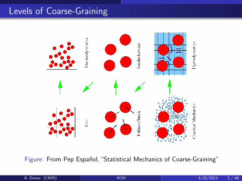
Levels of Coarse-Graining

Figure: From Pep Espanol, “Statistical Mechanics of Coarse-Graining”

A. Donev (CIMS) IICM 5/20/2013 3 / 46

Fluctuating Hydrodynamics

Continuum Models of Fluid Dynamics

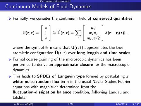
Formally, we consider the continuum field of conserved quantities

U(r, t) =

ρje

∼= U(r, t) =∑i

mi

miυi

miυ2i /2

δ [r − ri (t)] ,

where the symbol ∼= means that U(r, t) approximates the trueatomistic configuration U(r, t) over long length and time scales.

Formal coarse-graining of the microscopic dynamics has beenperformed to derive an approximate closure for the macroscopicdynamics.

This leads to SPDEs of Langevin type formed by postulating awhite-noise random flux term in the usual Navier-Stokes-Fourierequations with magnitude determined from thefluctuation-dissipation balance condition, following Landau andLifshitz.

A. Donev (CIMS) IICM 5/20/2013 5 / 46


Incompressible Fluctuating Navier-Stokes

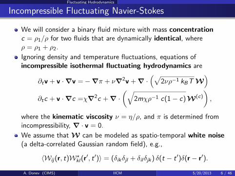
We will consider a binary fluid mixture with mass concentrationc = ρ1/ρ for two fluids that are dynamically identical, whereρ = ρ1 + ρ2.

Ignoring density and temperature fluctuations, equations ofincompressible isothermal fluctuating hydrodynamics are

∂tv + v ·∇v =−∇π + ν∇2v + ∇ ·(√

2νρ−1 kBT W)

∂tc + v ·∇c =χ∇2c + ∇ ·(√

2mχρ−1 c(1− c)W(c)

),

where the kinematic viscosity ν = η/ρ, and π is determined fromincompressibility, ∇ · v = 0.

We assume that W can be modeled as spatio-temporal white noise(a delta-correlated Gaussian random field), e.g.,

〈Wij(r, t)W?kl(r′, t ′)〉 = (δikδjl + δilδjk) δ(t − t ′)δ(r − r′).

A. Donev (CIMS) IICM 5/20/2013 6 / 46


Fluctuating Navier-Stokes Equations

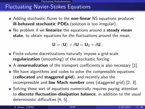
Adding stochastic fluxes to the non-linear NS equations producesill-behaved stochastic PDEs (solution is too irregular).

No problem if we linearize the equations around a steady meanstate, to obtain equations for the fluctuations around the mean,

U = 〈U〉+ δU = U0 + δU.

Finite-volume discretizations naturally impose a grid-scaleregularization (smoothing) of the stochastic forcing.

A renormalization of the transport coefficients is also necessary [1].

We have algorithms and codes to solve the compressible equations(collocated and staggered grid), and recently also theincompressible and low Mach number ones (staggered grid) [2, 3].

Solving these sort of equations numerically requires paying attentionto discrete fluctuation-dissipation balance, in addition to the usualdeterministic difficulties [4, 5].

A. Donev (CIMS) IICM 5/20/2013 7 / 46


Finite-Volume Schemes

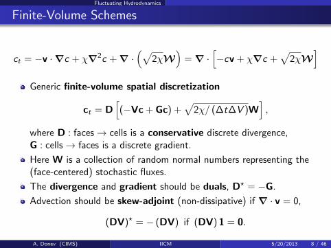
ct = −v ·∇c + χ∇2c + ∇ ·(√

2χW)

= ∇ ·[−cv + χ∇c +

√2χW

]Generic finite-volume spatial discretization

ct = D[(−Vc + Gc) +

√2χ/ (∆t∆V )W

],

where D : faces→ cells is a conservative discrete divergence,G : cells→ faces is a discrete gradient.

Here W is a collection of random normal numbers representing the(face-centered) stochastic fluxes.

The divergence and gradient should be duals, D? = −G.

Advection should be skew-adjoint (non-dissipative) if ∇ · v = 0,

(DV)? = − (DV) if (DV) 1 = 0.

A. Donev (CIMS) IICM 5/20/2013 8 / 46


Temporal Integration

∂tv = −∇π + ν∇2v + ∇ ·(√

2νρ−1 kBT W)

We use a Crank-Nicolson method for velocity with a Stokes solver forpressure:

vn+1 − vn

∆t+ Gπn+ 1

2 = νLv

(vn + vn+1

2

)+

(2νkBT

ρ∆t

) 12

DwWn

Dvn+1 = 0.

This coupled velocity-pressure Stokes linear system can be solvedefficiently even in the presence of non-periodic boundaries by using apreconditioned Krylov iterative solver.

The nonlinear terms such as v ·∇v and v ·∇c are handled explicitlyusing a predictor-corrector approach [5].

A. Donev (CIMS) IICM 5/20/2013 9 / 46


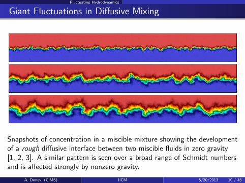
Giant Fluctuations in Diffusive Mixing

Snapshots of concentration in a miscible mixture showing the developmentof a rough diffusive interface between two miscible fluids in zero gravity[1, 2, 3]. A similar pattern is seen over a broad range of Schmidt numbersand is affected strongly by nonzero gravity.

A. Donev (CIMS) IICM 5/20/2013 10 / 46


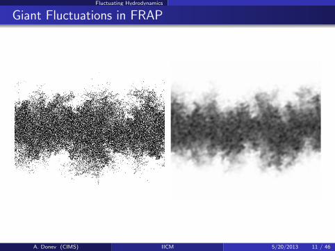
Giant Fluctuations in FRAP

A. Donev (CIMS) IICM 5/20/2013 11 / 46

Incompressible Inertial Coupling

Fluid-Structure Coupling

We want to construct a bidirectional coupling between a fluctuatingfluid and a small spherical Brownian particle (blob).

Macroscopic coupling between flow and a rigid sphere:

No-slip boundary condition at the surface of the Brownian particle.Force on the bead is the integral of the (fluctuating) stress tensor overthe surface.

The above two conditions are questionable at nanoscales, but evenworse, they are very hard to implement numerically in an efficient andstable manner.

We saw already that fluctuations should be taken into account atthe continuum level.

A. Donev (CIMS) IICM 5/20/2013 13 / 46


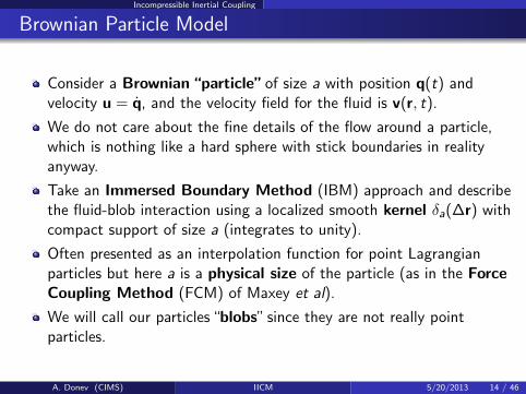
Brownian Particle Model

Consider a Brownian “particle” of size a with position q(t) andvelocity u = q, and the velocity field for the fluid is v(r, t).

We do not care about the fine details of the flow around a particle,which is nothing like a hard sphere with stick boundaries in realityanyway.

Take an Immersed Boundary Method (IBM) approach and describethe fluid-blob interaction using a localized smooth kernel δa(∆r) withcompact support of size a (integrates to unity).

Often presented as an interpolation function for point Lagrangianparticles but here a is a physical size of the particle (as in the ForceCoupling Method (FCM) of Maxey et al).

We will call our particles “blobs” since they are not really pointparticles.

A. Donev (CIMS) IICM 5/20/2013 14 / 46


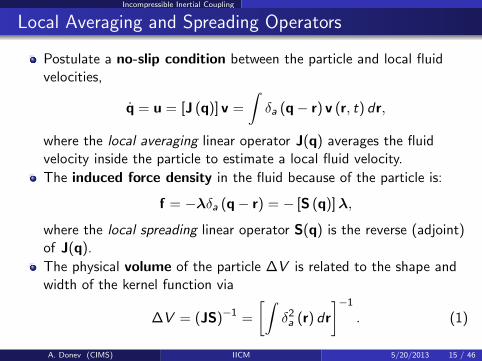
Local Averaging and Spreading Operators

Postulate a no-slip condition between the particle and local fluidvelocities,

q = u = [J (q)] v =

∫δa (q− r) v (r, t) dr,

where the local averaging linear operator J(q) averages the fluidvelocity inside the particle to estimate a local fluid velocity.

The induced force density in the fluid because of the particle is:

f = −λδa (q− r) = − [S (q)]λ,

where the local spreading linear operator S(q) is the reverse (adjoint)of J(q).

The physical volume of the particle ∆V is related to the shape andwidth of the kernel function via

∆V = (JS)−1 =

[∫δ2a (r) dr

]−1

. (1)

A. Donev (CIMS) IICM 5/20/2013 15 / 46


Fluid-Structure Direct Coupling

The equations of motion in our coupling approach are postulated tobe [6]

ρ (∂tv + v ·∇v) = −∇π −∇ · σ − [S (q)]λ+ ’thermal’ drift

me u = F (q) + λ

s.t. u = [J (q)] v and ∇ · v = 0,

where λ is the fluid-particle force, F (q) = −∇U (q) is theexternally applied force, and me is the excess mass of the particle.

The stress tensor σ = η(∇v + ∇Tv

)+ Σ includes viscous

(dissipative) and stochastic contributions. The stochastic stress

Σ = (kBTη)1/2 (W + WT)

drives the Brownian motion.

In the existing (stochastic) IBM approaches inertial effects areignored, me = 0 and thus λ = −F.

A. Donev (CIMS) IICM 5/20/2013 16 / 46


Momentum Conservation

In the standard approach a frictional (dissipative) forceλ = −ζ (u− Jv) is used instead of a constraint.

In either coupling the total particle-fluid momentum is conserved,

P = meu +

∫ρv (r, t) dr,

dP

dt= F.

Define a momentum field as the sum of the fluid momentum and thespreading of the particle momentum,

p (r, t) = ρv + meSu = (ρ+ meSJ) v.

Adding the fluid and particle equations gives a local momentumconservation law

∂tp = −∇π −∇ · σ −∇ ·[ρvvT + meS

(uuT

)]+ SF.

A. Donev (CIMS) IICM 5/20/2013 17 / 46


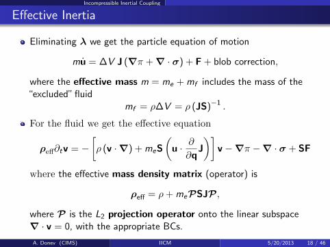
Effective Inertia

Eliminating λ we get the particle equation of motion

mu = ∆V J (∇π + ∇ · σ) + F + blob correction,

where the effective mass m = me + mf includes the mass of the“excluded” fluid

mf = ρ∆V = ρ (JS)−1 .

For the fluid we get the effective equation

ρeff∂tv = −[ρ (v ·∇) + meS

(u · ∂

∂qJ

)]v −∇π −∇ · σ + SF

where the effective mass density matrix (operator) is

ρeff = ρ+ mePSJP ,

where P is the L2 projection operator onto the linear subspace∇ · v = 0, with the appropriate BCs.

A. Donev (CIMS) IICM 5/20/2013 18 / 46


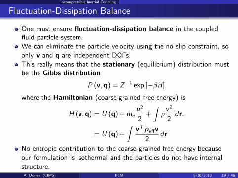
Fluctuation-Dissipation Balance

One must ensure fluctuation-dissipation balance in the coupledfluid-particle system.We can eliminate the particle velocity using the no-slip constraint, soonly v and q are independent DOFs.This really means that the stationary (equilibrium) distribution mustbe the Gibbs distribution

P (v,q) = Z−1 exp [−βH]

where the Hamiltonian (coarse-grained free energy) is

H (v,q) = U (q) + meu2

2+

∫ρ

v 2

2dr.

= U (q) +

∫vTρeffv

2dr

No entropic contribution to the coarse-grained free energy becauseour formulation is isothermal and the particles do not have internalstructure.

A. Donev (CIMS) IICM 5/20/2013 19 / 46


contd.

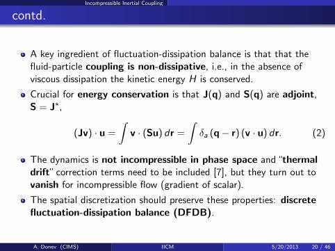
A key ingredient of fluctuation-dissipation balance is that that thefluid-particle coupling is non-dissipative, i.e., in the absence ofviscous dissipation the kinetic energy H is conserved.

Crucial for energy conservation is that J(q) and S(q) are adjoint,S = J?,

(Jv) · u =

∫v · (Su) dr =

∫δa (q− r) (v · u) dr. (2)

The dynamics is not incompressible in phase space and “thermaldrift” correction terms need to be included [7], but they turn out tovanish for incompressible flow (gradient of scalar).

The spatial discretization should preserve these properties: discretefluctuation-dissipation balance (DFDB).

A. Donev (CIMS) IICM 5/20/2013 20 / 46

Numerics

Numerical Scheme

Both compressible (explicit) and incompressible schemes have beenimplemented by Florencio Balboa (UAM) on GPUs.

Spatial discretization is based on previously-developed staggeredschemes for fluctuating hydro [2] and the IBM kernel functions ofCharles Peskin.

Temporal discretization follows a second-order splitting algorithm(move particle + update momenta), and is limited in stability only byadvective CFL.

The scheme ensures strict conservation of momentum and (almostexactly) enforces the no-slip condition at the end of the time step.

Continuing work on temporal integrators that ensure the correctequilibrium distribution and diffusive (Brownian) dynamics.

A. Donev (CIMS) IICM 5/20/2013 22 / 46

Numerics

Spatial Discretization

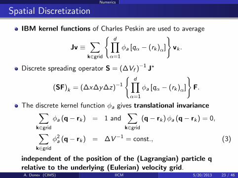
IBM kernel functions of Charles Peskin are used to average

Jv ≡∑

k∈grid

d∏

α=1

φa [qα − (rk)α]

vk .

Discrete spreading operator S = (∆Vf )−1 J?

(SF)k = (∆x∆y∆z)−1

d∏

α=1

φa [qα − (rk)α]

F.

The discrete kernel function φa gives translational invariance∑k∈grid

φa (q− rk) = 1 and∑

k∈grid

(q− rk)φa (q− rk) = 0,

∑k∈grid

φ2a (q− rk) = ∆V−1 = const., (3)

independent of the position of the (Lagrangian) particle qrelative to the underlying (Eulerian) velocity grid.

A. Donev (CIMS) IICM 5/20/2013 23 / 46

Numerics

Temporal Discretization

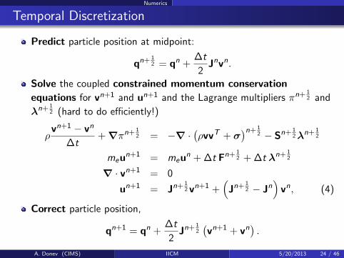
Predict particle position at midpoint:

qn+ 12 = qn +

∆t

2Jnvn.

Solve the coupled constrained momentum conservation

equations for vn+1 and un+1 and the Lagrange multipliers πn+ 12 and

λn+ 12 (hard to do efficiently!)

ρvn+1 − vn

∆t+ ∇πn+ 1

2 = −∇ ·(ρvvT + σ

)n+ 12 − Sn+ 1

2λn+ 12

meun+1 = meun + ∆t Fn+ 12 + ∆t λn+ 1

2

∇ · vn+1 = 0

un+1 = Jn+ 12 vn+1 +

(Jn+ 1

2 − Jn)

vn, (4)

Correct particle position,

qn+1 = qn +∆t

2Jn+ 1

2(vn+1 + vn

).

A. Donev (CIMS) IICM 5/20/2013 24 / 46

Numerics

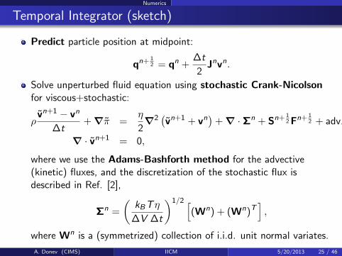
Temporal Integrator (sketch)

Predict particle position at midpoint:

qn+ 12 = qn +

∆t

2Jnvn.

Solve unperturbed fluid equation using stochastic Crank-Nicolsonfor viscous+stochastic:

ρvn+1 − vn

∆t+ ∇π =

η

2∇2(vn+1 + vn

)+ ∇ ·Σn + Sn+ 1

2 Fn+ 12 + adv.,

∇ · vn+1 = 0,

where we use the Adams-Bashforth method for the advective(kinetic) fluxes, and the discretization of the stochastic flux isdescribed in Ref. [2],

Σn =

(kBTη

∆V ∆t

)1/2 [(Wn) + (Wn)T

],

where Wn is a (symmetrized) collection of i.i.d. unit normal variates.

A. Donev (CIMS) IICM 5/20/2013 25 / 46

Numerics

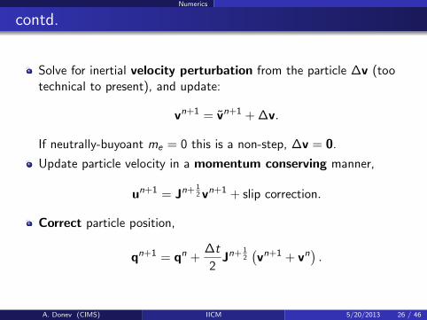
contd.

Solve for inertial velocity perturbation from the particle ∆v (tootechnical to present), and update:

vn+1 = vn+1 + ∆v.

If neutrally-buyoant me = 0 this is a non-step, ∆v = 0.

Update particle velocity in a momentum conserving manner,

un+1 = Jn+ 12 vn+1 + slip correction.


qn+1 = qn +∆t

2Jn+ 1

2(vn+1 + vn

).

A. Donev (CIMS) IICM 5/20/2013 26 / 46

Numerics

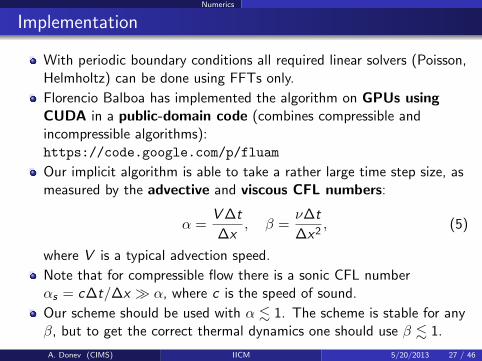
Implementation

With periodic boundary conditions all required linear solvers (Poisson,Helmholtz) can be done using FFTs only.

Florencio Balboa has implemented the algorithm on GPUs usingCUDA in a public-domain code (combines compressible andincompressible algorithms):https://code.google.com/p/fluam

Our implicit algorithm is able to take a rather large time step size, asmeasured by the advective and viscous CFL numbers:

α =V ∆t

∆x, β =

ν∆t

∆x2, (5)

where V is a typical advection speed.

Note that for compressible flow there is a sonic CFL numberαs = c∆t/∆x α, where c is the speed of sound.

Our scheme should be used with α . 1. The scheme is stable for anyβ, but to get the correct thermal dynamics one should use β . 1.

A. Donev (CIMS) IICM 5/20/2013 27 / 46

https://code.google.com/p/fluam

Results

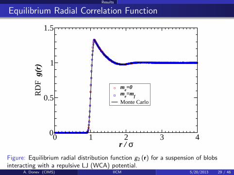
Equilibrium Radial Correlation Function

0 1 2 3 4r / σ

0

0.5

1

1.5R

DF

g(r

)

me=0me=mf

Monte Carlo

Figure: Equilibrium radial distribution function g2 (r) for a suspension of blobsinteracting with a repulsive LJ (WCA) potential.

A. Donev (CIMS) IICM 5/20/2013 29 / 46

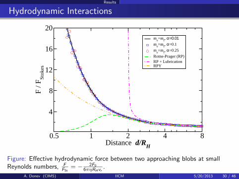
Results

Hydrodynamic Interactions

0.5 1 2 4 8Distance d/RH

4

8

12

16

20F

/ FSt

okes

me=m

f, α=0.01

me=m

f, α=0.1

me=m

f, α=0.25

Rotne-Prager (RP)RP + LubricationRPY

Figure: Effective hydrodynamic force between two approaching blobs at smallReynolds numbers, F

FSt= − 2F0

6πηRHvr.

A. Donev (CIMS) IICM 5/20/2013 30 / 46

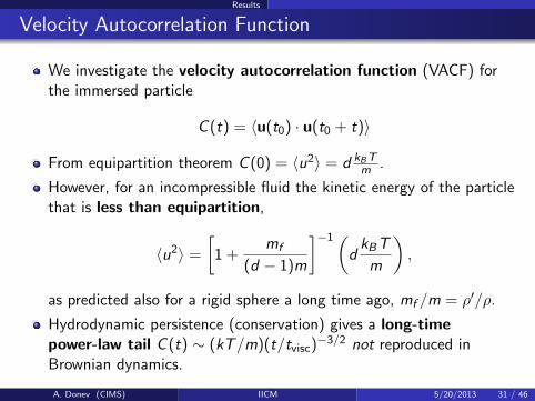
Results

Velocity Autocorrelation Function

We investigate the velocity autocorrelation function (VACF) forthe immersed particle

C (t) = 〈u(t0) · u(t0 + t)〉

From equipartition theorem C (0) = 〈u2〉 = d kBTm .

However, for an incompressible fluid the kinetic energy of the particlethat is less than equipartition,

〈u2〉 =

[1 +

mf

(d − 1)m

]−1(d

kBT

m

),

as predicted also for a rigid sphere a long time ago, mf /m = ρ′/ρ.

Hydrodynamic persistence (conservation) gives a long-timepower-law tail C (t) ∼ (kT/m)(t/tvisc)−3/2 not reproduced inBrownian dynamics.

A. Donev (CIMS) IICM 5/20/2013 31 / 46

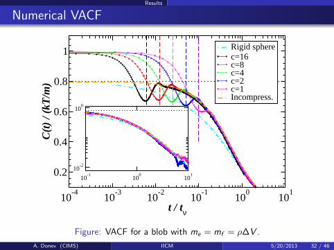
Results

Numerical VACF

10-4

10-3

10-2

10-1

100

101

t / tν

0.2

0.4

0.6

0.8

1C

(t)

/ (kT

/m)

Rigid spherec=16c=8c=4c=2c=1Incompress.

10-1

100

101

10-2

100

Figure: VACF for a blob with me = mf = ρ∆V .

A. Donev (CIMS) IICM 5/20/2013 32 / 46

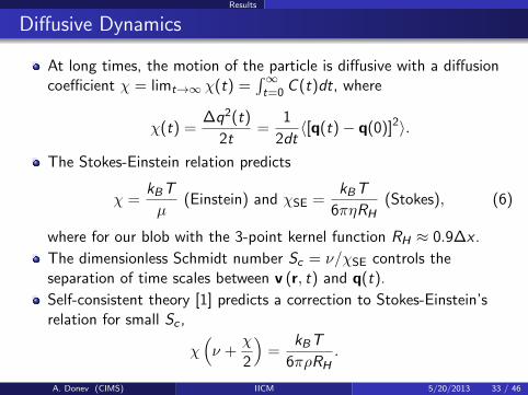
Results

Diffusive Dynamics

At long times, the motion of the particle is diffusive with a diffusioncoefficient χ = limt→∞ χ(t) =

∫∞t=0 C (t)dt, where

χ(t) =∆q2(t)

2t=

1

2dt〈[q(t)− q(0)]2〉.

The Stokes-Einstein relation predicts

χ =kBT

µ(Einstein) and χSE =

kBT

6πηRH(Stokes), (6)

where for our blob with the 3-point kernel function RH ≈ 0.9∆x .

The dimensionless Schmidt number Sc = ν/χSE controls theseparation of time scales between v (r, t) and q(t).

Self-consistent theory [1] predicts a correction to Stokes-Einstein’srelation for small Sc ,

χ(ν +

χ

2

)=

kBT

6πρRH.

A. Donev (CIMS) IICM 5/20/2013 33 / 46

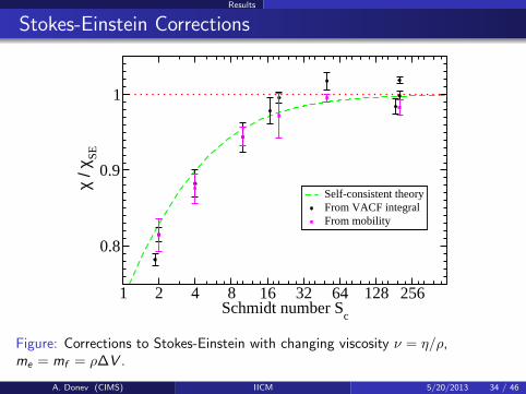
Results

Stokes-Einstein Corrections

1 2 4 8 16 32 64 128 256Schmidt number S

c

0.8

0.9

1 χ

/ χ SE

Self-consistent theoryFrom VACF integralFrom mobility

Figure: Corrections to Stokes-Einstein with changing viscosity ν = η/ρ,me = mf = ρ∆V .

A. Donev (CIMS) IICM 5/20/2013 34 / 46

Results

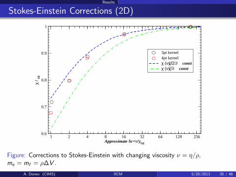
Stokes-Einstein Corrections (2D)

1 2 4 8 16 32 64 128 256Approximate Sc=ν/χSE

0.6

0.7

0.8

0.9

1

χ / SE

3pt kernel4pt kernelχ (ν+χ/2) = constχ (ν+χ) = const

Figure: Corrections to Stokes-Einstein with changing viscosity ν = η/ρ,me = mf = ρ∆V .

A. Donev (CIMS) IICM 5/20/2013 35 / 46

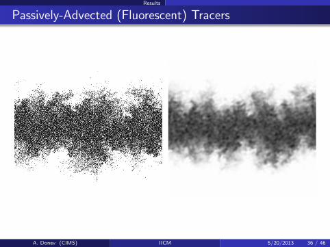
Results

Passively-Advected (Fluorescent) Tracers

A. Donev (CIMS) IICM 5/20/2013 36 / 46

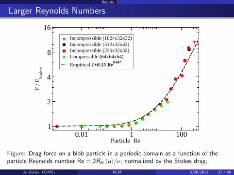
Results

Larger Reynolds Numbers

0.01 1 100Particle Re

1

2

4

8

16F

/ FSt

okes

Incompressible (1024x32x32)Incompressible (512x32x32)Incompressible (256x32x32)Compressible (64x64x64)

Empirical 1+0.15 Re0.687

Figure: Drag force on a blob particle in a periodic domain as a function of theparticle Reynolds number Re = 2RH 〈u〉/ν, normalized by the Stokes drag.

A. Donev (CIMS) IICM 5/20/2013 37 / 46

Outlook

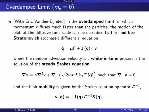
Overdamped Limit (me = 0)

[With Eric Vanden-Eijnden] In the overdamped limit, in whichmomentum diffuses much faster than the particles, the motion of theblob at the diffusive time scale can be described by the fluid-freeStratonovich stochastic differential equation

q = µF + J (q) v

where the random advection velocity is a white-in-time process is thesolution of the steady Stokes equation

∇π = ν∇2v + ∇ ·(√

2νρ−1 kBT W)

such that ∇ · v = 0,

and the blob mobility is given by the Stokes solution operator L−1,

µ (q) = −J (q)L−1S (q) .

A. Donev (CIMS) IICM 5/20/2013 39 / 46

Outlook

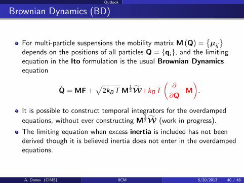
Brownian Dynamics (BD)

For multi-particle suspensions the mobility matrix M (Q) =µij

depends on the positions of all particles Q = qi, and the limitingequation in the Ito formulation is the usual Brownian Dynamicsequation

Q = MF +√

2kBT M12W+kBT

(∂

∂Q·M).

It is possible to construct temporal integrators for the overdamped

equations, without ever constructing M12W (work in progress).

The limiting equation when excess inertia is included has not beenderived though it is believed inertia does not enter in the overdampedequations.

A. Donev (CIMS) IICM 5/20/2013 40 / 46

Outlook

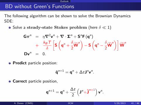
BD without Green’s Functions

The following algorithm can be shown to solve the Brownian DynamicsSDE:

Solve a steady-state Stokes problem (here δ 1)

Gπn = η∇2vn + ∇ ·Σn + SnF (qn)

+kBT

δ

[S

(qn +

δ

2W

n)− S

(qn − δ

2W

n)]

Wn

Dvn = 0.

Predict particle position:

qn+1 = qn + ∆tJnvn.


qn+1 = qn +∆t

2

(Jn+J

n+1)

vn.

A. Donev (CIMS) IICM 5/20/2013 41 / 46

Outlook

Immersed Rigid Blobs

Unlike a rigid sphere, a blob particle would not perturb a pure shearflow.

In the far field our blob particle looks like a force monopole(stokeset), and does not exert a force dipole (stresslet) on the fluid.

Similarly, since here we do not include angular velocity degrees offreedom, our blob particle does not exert a torque on the fluid(rotlet).

It is possible to include rotlet and stresslet terms, as done in the forcecoupling method [8] and Stokesian Dynamics in the deterministicsetting.

Proper inclusion of inertial terms and fluctuation-dissipation balancenot studied carefully yet...

A. Donev (CIMS) IICM 5/20/2013 42 / 46

Outlook

Immersed Rigid Bodies

This approach can be extended to immersed rigid bodies (work withNeelesh Patankar)

ρ (∂tv + v ·∇v) = −∇π −∇ · σ −∫

ΩS (q)λ (q) dq + th. drift

me u = F +

∫Ωλ (q) dq

Ieω = τ +

∫Ω

[q× λ (q)] dq

[J (q)] v = u + q× ω for all q ∈ Ω

∇ · v = 0 everywhere.

Here ω is the immersed body angular velocity, τ is the applied torque,and Ie is the excess moment of inertia of the particle.The nonlinear advective terms are tricky, though it may not be aproblem at low Reynolds number...Fluctuation-dissipation balance needs to be studied carefully...

A. Donev (CIMS) IICM 5/20/2013 43 / 46

Outlook

Conclusions

Fluctuations are not just a microscopic phenomenon: giantfluctuations can reach macroscopic dimensions or certainly dimensionsmuch larger than molecular.

Fluctuating hydrodynamics seems to be a very good coarse-grainedmodel for fluids, and coupled to immersed particles to modelBrownian suspensions.

The minimally-resolved blob approach provides a low-cost butreasonably-accurate representation of rigid particles in flow.

We have recently successfully extended the blob approach toreaction-diffusion problems (with Amneet Bhalla and NeeleshPatankar).

Particle inertia can be included in the coupling between blobparticles and a fluctuating incompressible fluid.

More complex particle shapes can be built out of a collection ofblobs.

A. Donev (CIMS) IICM 5/20/2013 44 / 46

Outlook

Reactive Blobs

Continuum: Diffusion equation for the concentration of the speciesc (r, t),

∂tc = χ∇2c + s (r, t) in Ω \ S, (7)

χ (n ·∇c) = k c on ∂S, (8)

where k is the surface reaction rate.

Reactive-blob model

∂tc = χ∇2c − κ[∫

δa (q− r) c (r, t) dr

]δa (q− r) + s,

and discretization

∂tc = χ∇2c − κSJc + s,

where κ = 4πka2 is the overall reaction rate.

Requires specialized linear solvers in the diffusion-limited regime.

A. Donev (CIMS) IICM 5/20/2013 45 / 46

Outlook

References

A. Donev, A. L. Garcia, Anton de la Fuente, and J. B. Bell.

Enhancement of Diffusive Transport by Nonequilibrium Thermal Fluctuations.J. of Statistical Mechanics: Theory and Experiment, 2011:P06014, 2011.

F. Balboa Usabiaga, J. B. Bell, R. Delgado-Buscalioni, A. Donev, T. G. Fai, B. E. Griffith, and C. S. Peskin.

Staggered Schemes for Incompressible Fluctuating Hydrodynamics.SIAM J. Multiscale Modeling and Simulation, 10(4):1369–1408, 2012.

A. Donev, A. J. Nonaka, Y. Sun, T. Fai, A. L. Garcia, and J. B. Bell.

Low Mach Number Fluctuating Hydrodynamics of Diffusively Mixing Fluids.Submitted to SIAM J. Multiscale Modeling and Simulation, 2013.

A. Donev, E. Vanden-Eijnden, A. L. Garcia, and J. B. Bell.

On the Accuracy of Explicit Finite-Volume Schemes for Fluctuating Hydrodynamics.CAMCOS, 5(2):149–197, 2010.

S. Delong, B. E. Griffith, E. Vanden-Eijnden, and A. Donev.

Temporal Integrators for Fluctuating Hydrodynamics.Phys. Rev. E, 87(3):033302, 2013.

F. Balboa Usabiaga, R. Delgado-Buscalioni, B. E. Griffith, and A. Donev.

Inertial Coupling Method for particles in an incompressible fluctuating fluid.Submitted, code available at https://code.google.com/p/fluam/, 2013.

P. J. Atzberger.

Stochastic Eulerian-Lagrangian Methods for Fluid-Structure Interactions with Thermal Fluctuations.J. Comp. Phys., 230:2821–2837, 2011.

S. Lomholt and M.R. Maxey.

Force-coupling method for particulate two-phase flow: Stokes flow.J. Comp. Phys., 184(2):381–405, 2003.

A. Donev (CIMS) IICM 5/20/2013 46 / 46

https://code.google.com/p/fluam/

Coupling an Incompressible Fluctuating Fluid with...

Documents

Transcript of Coupling an Incompressible Fluctuating Fluid with...