L3: Risk and Risk Measurement 1 Risk and Risk Measurement (L3) Following topics are covered: –Risk...

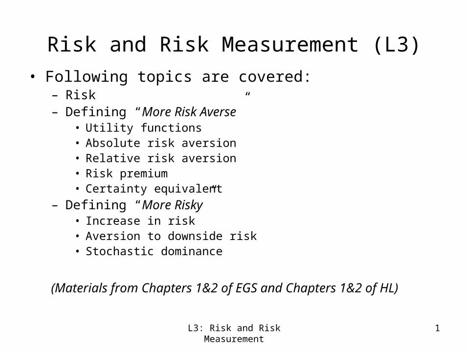
L3: Risk and Risk Measurement 1

Risk and Risk Measurement (L3)

• Following topics are covered:– Risk – Defining “More Risk Averse”

• Utility functions• Absolute risk aversion• Relative risk aversion• Risk premium• Certainty equivalent

– Defining “More Risky”• Increase in risk• Aversion to downside risk• Stochastic dominance

(Materials from Chapters 1&2 of EGS and Chapters 1&2 of HL)


Risk• Risk can be generally defined as “uncertainty”.• Sempronius owns goods at home worth a total of 4000 ducats and in

addition possesses 8000 decats worth of commodities in foreign countries from where they can only be transported by sea, with ½ chance that the ship will perish.

• If he puts all the foreign commodity in 1 ship, this wealth, represented by a lottery, is x ~ (4000, ½; 12000, ½)

• If he put the foreign commodity in 2 ships, assuming the ships follow independent but equally dangerous routes. Sempronius faces a more diversified lottery y ~ (4000, ¼; 8000, ½; 12000, ¼)

• In either case, Sempronius faces a risk on his wealth. What are the expected values of these two lotteries?

• In reality, most people prefer the latter. Why?

St. Petersburg Paradox

• You pay a fixed fee to enter and then a fair coin is tossed repeatedly until a tail appears, ending the game. The pot starts at 1 dollar is doubled every time a head appears. You win whatever is in the pot after the game ends. What is the fair price to pay for entering the game?

• Are you willing to pay this?

• See page 13, HL.L3: Risk and Risk Measurement 3


Risk Aversion and Utility Function• A risk-averse agent is an agent who dislikes zero-mean

risks.• Risk aversion:

– Utility function is the relationship between monetary outcome, x, and the degree of satisfaction, u(x).

• Concavity– a twice-differentiable function u is concave if and only if its second

derivative is negative, i.e., if the marginal utility u’(x) is decreasing in x.

– E.g, u(x)=ln(x)• A decision maker is risk-averse the agent’s utility

function u is concave. – proposition 2, page 8, EGS– Be able to prove this

• Jensen Inequality

)()( EzwuzwEu .


Von Neumann_Morgenstern Utility Function

von Neumann-Morgenstern utility describes a utility function (or perhaps a broader class of preference relations) that has the expected utility property: the agent is indifferent between receiving a given bundle or a gamble with the same expected value.


Risk Premium and Certainty Equivalent

• Risk Premium– Risk-averse investors may want to purchase risky assets if their

expected return exceed the risk-free rate.

– Eu(w+z)=u(w-Π), where z is a zero-mean risk, w is the initial wealth

– Π is risk premium – cost of risk

• Certainty equivalent – The amount of payoff (e.g. money or utility) that an agent would

have to receive to be indifferent between that payoff and a given gamble

– What is certainty equivalent in the above expression?

• Arrow-Pratt approximation of risk premium– where A(w)=-u’’(w)/u(w))(

2

1 2 wA


Deriving Risk Premium (Arrow_Pratt Approximation)

)(''2

1)(

)(''2

1)(')(

)](''2

1)(')([)(

2

2

2

wuwu

wuEzEzwuwu

wuzwzuwuEzwEu

where Ez=0 and variance σ2=Ez2. Also note that Eu(w+z) = u(w-П), where u(w- П) = u(w)- Пu’(w). Thus proved.

Note: The cost of risk, as measured by risk premium, is approximately proportional to the variance of its payoffs. This is one reason why researchers use a mean-variance decision criterion for modeling behavior under risk. However П=1/2σ2*A(w) only holds for small risk (thus we can apply for the 2nd-order approximation).


Further discussions

• Arrow-Pratt expression of risk premium works for small risk or special utility functions where only mean and variance are applicable to the expected utility– See page 20, quadratic utility function


Measuring Risk Aversion• The degree of absolute risk aversion

• For small risks, the risk premium increases with the size of the risk proportionately to the square of the size– Assuming z=k*ε, where E(ε)=0, σ(ε)=σ

• Accepting a small-mean risk has no effect on the wealth of risk-averse agents

• ARA is a measure of the degree of concavity of a utility function, i.e., the speed at which marginal utility decreases

)('

)('')(

wu

wuwA

)(2

1 22 wAk


More Risk Averse Agent

• Consider two risk averse agents u and v. if v is more risk averse than u, this is equivalent to that Av>Au

Proof: Suppose v is a concave transformation of u. I.e., v(w) = φ(u(w)), We have v’(w) = φ’(u(w))u’(w). Hence, v’’(w)= φ’’(u(w))(u’(w))2 +φ’(u(w))u’’(w),

We have ))(('

)('))(('')()(

wu

wuwuwAwA uv

• Conditions leading to more risk Aversion – page 14-15


Example

• Two agents’ utility functions are u(w) and v(w). u(w)= w , v(w)=ln(w);

(1) Which agent is more risk averse in small risks and in large risks? (2) Suppose they have an initial wealth of 4000 ducats and face a risk

of (0, ½; 8000, ½). Find their respective risk premiums.


CARA and DARA• CARA

• However, ARA typically decreases– Assuming for a square root utility function, what would be the risk premium

of an individual having a wealth of dollar 101 versus a guy whose wealth is dollar 100000 with a lottery to gain or lose $100 with equal probability?

• What kind of utility function has a decreasing risk premium?

Eu(w+z)=u(w-π(w)) Eu’(w+z)=(1- π’(w))u’(w-π(w))

)('

)(')(')('

wu

zwEuwuw

u(w) is an increasing and concave utility function, thus, u’(.)>0 to have a decreasing risk premium in w, we need u’(w- π)≤ Eu’(w+z) Defining v=-u’, we have the following condition for decreasing risk premium Ev(w+z) ≤v(w- π) The above condition states that ????


Prudence

• Thus –u’ is a concave transformation of u.• Defining risk aversion of (-u’) as –u’’’/u’’• This is known as prudence, P(w)• The risk premium associated to any risk z is decreasing in

wealth if and only if absolute risk aversion is decreasing or prudence is uniformly larger than absolute risk aversion

• P(w)≥A(w)


Relative Risk Aversion

• Definition

• Using z for proportion risk, the relation between relative risk premium, ПR(z), and absolute risk premium, ПA(wz) is

• This can be used to establish a reasonable range of risk aversion: given that (1) investors have a lottery of a gain or loss of 20% with equal probability and (2) most people is willing to pay between 2% and 8% of their wealth (page 18, EGS).

• CRRA

)()('

)(''

/

)('/)(')( wwA

wu

wwu

wdw

wuwduwR

)(2

1)()( 2 wR

w

wzz

AR


Some Classical Utility Function

A. Quadratic function: u(w)=aw-1/2w2 – increasing absolute risk aversion

B. Exponential function: a

awwu

)exp()(

-- constant absolute risk aversion

C. Power utility function:

1)(

1wwu -- constant relative risk aversion

D. log utility function: u(w) = ln(w) – constant relative risk aversion

For more of utility functions commonly used, see HL, pages 25-28

Also see HL, Page 11 for von Neumann-Morgenstern utility, i.e., utility function having expected value

Appropriate expression of expected utility, see HL, page 6 and 7


Measuring Risks

• So far, we discuss investors’ attitude on risk when risk is given– I.e., investors have different utility functions, how a give risk affects

investors’ wealth

• Now we move to risk itself – how does a risk change?

• Definition: A wealth distributions w1 is preferred to w2, when Eu(w1)≥Eu(w2)– Increasing risk in the sense of Rothschild and Stiglitz (1970)

– An increase in downside risk (Menezes, Geiss and Tressler (1980))

– First-order stochastic dominance


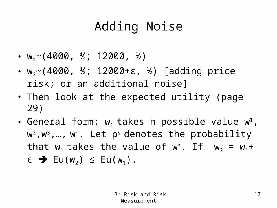
Adding Noise

• w1~(4000, ½; 12000, ½)

• w2~(4000, ½; 12000+ε, ½) [adding price risk; or an additional noise]

• Then look at the expected utility (page 29)

• General form: w1 takes n possible value w1, w2,w3,…, wn. Let ps

denotes the probability that w1 takes the value of ws. If w2 = w1+ ε Eu(w2) ≤ Eu(w1).


Mean Preserving Spread Transformation

• Definition:

– Assuming all possible final wealth levels are in interval [a,b] and I is a subset of [a, b]

– Let fi(w) denote the probability mass of w2 (i=1, 2) at w. w2 is a mean-preserving spread (MPS) of w1 if

1. Ew2= Ew1

2. There exists an interval I such that f2(w)≤ f1(w) for all w in I

• Example: the figure in the left-handed panel of page 31

• Increasing noise and mean preserving spread (MPS) are equivalent


Single Crossing Property• Mean Preserving spread implies that (integration by parts – page 31)

• This implies a “single-crossing” property: F2 must be larger than F1 to the left of some threshold w and F2 must be smaller than F1 to its right. I.e.,

b

adssFsF 0)]()([ 12

w

adssFsFws 0)]()([)( 12


The Integral Condition

b

a

b

a ibwawiii dwwFwuwFwudwwfwuwEu )()('|)()()()()(

I.e., dwwFwubuwEub

a ii )()(')()(

It follows that: dwwFwFwuwEuwEub

a)]()()[(')()( 2112 -- page 32 for

interpretation Integrating by parts yields

dwdwwFwFwuwSwuwEuwEub

a

b

a

ba ))]()([)((''|)()(')()( 2112

Thus dwwSwuwEuwEub

a )()('')()( 12

For a risk averse agent, the above expressive is uniformly negative.


MPS Conditions

Consider two random variable w1 and w2 with the same mean,

(1) All risk averse agents prefer w1 to w2 for all concave function u

(2) w2 is obtained from w1 by adding zero-mean noise to the possible outcome of w1

(3) w2 is obtained w1 by a sequence of mean-preserving spreads

(4) S(w)≥0 holds for all w.


Preference for Diversification

• Suppose Sempreonius has an initial wealth of w (in term of pounds of spicy). He ships 8000 pounds oversea. Also suppose the probability of a ship being sunk is ½. x takes 0 if the ship sinks and 1 otherwise. If putting spicy in 1 ship, his final wealth is w2=w+8000*x

• If he puts spicy in 2 ships, his final wealth is w1=w+8000(x1+x2)/2

• Sempreonius would prefer two ships as long as his utility function is concave

• Diversification is a risk-reduction device in the sense of Rothschild of Stiglitz (1970).


Variance and Preference

• Two risky assets, w1 and w2, w1 is preferred to w2 iff П2> П1• For a small risk, w1 is preferred to w2 iff the variance of w2

exceeds the variance of w1

• But this does not hold for a large risk. The correct statement is that all risk-averse agents with a quadratic utility function prefer w1 to w2 iff the variance of the second is larger than the variance of the first– See page 35.


Aversion to Downside Risk

• Definition: agents dislike transferring a zero-mean risk from a richer to a poor state.

• w2~(4000, ½; 12000+ε, ½)

• w3~(4000+ ε, ½; 12000, ½)

• Which is more risky

• Depends, generally agents dislike risks in lower states more. But it depends on agents’ utility function


First-Degree Stochastic Dominance• Definition: w2 is dominated by w1 in the sense of the first-

degree stochastic dominance order if F2(w)≥F1(w) for all w.

• Consumers would dislike FSD-dominated shifts in the distribution final wealth

• No longer mean preserving

0)]()()[('

)]()()[()()(

21

1212

dwwFwFwu

dwwfwfwuwEuwEu

b

a

b

a

F(w)

w

W2

W1


Equivalent Conditions on FSD• All agents with a nondecreasing utility function prefer w1

to w2: Eu(w2)<=Eu(w1) for all nondecreasing functions u, or stated as,

• W2 is dominated w1 in the sense of FSD: w2 is obtained from w1 by a transfer of probability mass from the high wealth states to lower wealth states, or F2(w)≥F1(w) for all w.

• W1 is obtained from w2 by adding nonnegative noise terms to the possible outcome of w2: where є is no less than 0 with probability one.

21 wwFSD

21 wwd


Second-degree Stochastic Dominance

• Definition

– w1 dominates w2 in the sense of the second-degree stochastic dominance if and only if

– This is same mean preserving spread or adding a noise; see page 49, HL.

]1,0[0)]()([)(

)()(

0 21

21

ydzwFwFys

wEwEy

Allais Paradox

• The Allais paradox is a choice problem designed by Maurice Allais to show an inconsistency of actual observed choices with the predictions of expected utility theory.

• Two pairs of games

• What is your choice?


http://en.wikipedia.org/wiki/Maurice_Allais

Ellsberg Paradox (Ambiguity Aversion)• The Ellsberg paradox is a paradox in decision theory and experimental

economics in which people’s choices violate the expected utility hypothesis. It is generally taken to be evidence for ambiguity aversion.

• The 1urn paradox: suppose you have an urn containing 30 red balls and 60 other balls that are either black or yellow. You don't know how many black or yellow balls there are, but that the total number of black balls plus the total number of yellow equals 60. The balls are well mixed so that each individual ball is as likely to be drawn as any other.

• You are now given a choice:– Gamble A: You receive $100 if you draw a red ball

– Gamble B: You receive $100 if you draw a black ball

• Also you are given options between Gamble C and D– You receive $100 if you draw a red or yellow ball

– You receive $100 if you draw a black or yellow ball



Technical Notes

• Taylor Series Expansion: f(x)=

• Integration by parts

which in a more compact form can be written


Exercises

• EGS, 1.2; 1.4; 2.2

L3: Risk and Risk Measurement 1 Risk and Risk Measurement (L3) Following topics are covered: –Risk...

Documents

Transcript of L3: Risk and Risk Measurement 1 Risk and Risk Measurement (L3) Following topics are covered: –Risk...