Financial Risk Measurement

for

Financial Risk Management∗

Torben G. Andersen† Tim Bollerslev‡

Northwestern University Duke University

Peter F. Christoffersen§ Francis X. Diebold¶

University of Toronto University of Pennsylvania

November 2, 2011

Abstract

Current practice largely follows restrictive approaches to market risk mea-

surement, such as historical simulation or RiskMetrics. In contrast, we propose

flexible methods that exploit recent developments in financial econometrics and

are likely to produce more accurate risk assessments, treating both portfolio-

level and asset-level analysis. Asset-level analysis is particularly challenging

because the demands of real-world risk management in financial institutions

– in particular, real-time risk tracking in very high-dimensional situations –

impose strict limits on model complexity. Hence we stress powerful yet parsi-

monious models that are easily estimated. In addition, we emphasize the need

for deeper understanding of the links between market risk and macroeconomic

fundamentals, focusing primarily on links among equity return volatilities, real

growth, and real growth volatilities. Throughout, we strive not only to deepen

our scientific understanding of market risk, but also cross-fertilize the academic

and practitioner communities, promoting improved market risk measurement

technologies that draw on the best of both.

∗This paper is prepared for G. Constantinedes, M. Harris and Rene Stulz (eds.), Handbook of theEconomics of Finance, Elsevier. For helpful comments we thank Hal Cole and Dongho Song. Forresearch support, Andersen, Bollerslev and Diebold thank the National Science Foundation (U.S.),and Christoffersen thanks the Social Sciences and Humanities Research Council (Canada).

†Torben G. Andersen is Nathan and Mary Sharp Distinguished Professor of Financeat the Kellogg School of Management, Northwestern University, Research Associate atthe NBER, and International Fellow of CREATES, University of Aarhus, Denmark. t-andersen@kellogg.northwestern.edu.

‡Tim Bollerslev is Juanita and Clifton Kreps Professor of Economics, Duke University, Professorof Finance at its Fuqua School of Business, Research Associate at the NBER, and an InternationalFellow of CREATES, University of Aarhus, Denmark. boller@econ.duke.edu.

§Peter F. Christoffersen is Professor of Finance at the Rotman School of Management, Universityof Toronto and affiliated with Copenhagen Business School and CREATES, University of Aarhus,Denmark. peter.christoffersen@rotman.utoronto.ca.

¶Francis X. Diebold is Paul F. and Warren S. Miller Professor of Economics at the Universityof Pennsylvania, Professor of Finance and Statistics and Co-Director of the Financial InstitutionsCenter at its Wharton School, and Research Associate at the NBER. fdiebold@wharton.upenn.edu.

Contents

1 Introduction 1

1.1 Six Emergent Themes . . . . . . . . . . . . . . . . . . . . . . . . . . 1

1.2 Conditional Risk Measures . . . . . . . . . . . . . . . . . . . . . . . . 2

1.3 Plan of the Chapter . . . . . . . . . . . . . . . . . . . . . . . . . . . . 6

2 Conditional Portfolio-Level Risk Analysis 7

2.1 Modeling Time-Varying Volatilities Using Daily Data and GARCH . 8

2.1.1 Exponential Smoothing and RiskMetrics . . . . . . . . . . . . 8

2.1.2 The GARCH(1,1) Model . . . . . . . . . . . . . . . . . . . . . 11

2.1.3 Extensions of the Basic GARCH Model . . . . . . . . . . . . . 14

2.2 Intraday Data and Realized Volatility . . . . . . . . . . . . . . . . . . 18

2.2.1 Dynamic Modeling of Realized Volatility . . . . . . . . . . . . 23

2.2.2 Realized Volatilities and Jumps . . . . . . . . . . . . . . . . . 29

2.2.3 Combining GARCH and RV . . . . . . . . . . . . . . . . . . . 33

2.3 Modeling Return Distributions . . . . . . . . . . . . . . . . . . . . . . 36

2.3.1 Procedures Based on GARCH . . . . . . . . . . . . . . . . . 41

2.3.2 Procedures Based on Realized Volatility . . . . . . . . . . . . 43

2.3.3 Combining GARCH and RV . . . . . . . . . . . . . . . . . . . 45

2.3.4 Simulation Methods . . . . . . . . . . . . . . . . . . . . . . . 46

2.3.5 Extreme Value Theory . . . . . . . . . . . . . . . . . . . . . . 48

3 Conditional Asset-Level Risk Analysis 49

3.1 Modeling Time-Varying Covariances Using Daily Data and GARCH . 51

3.1.1 Dynamic Conditional Correlation Models . . . . . . . . . . . . 54

3.1.2 Factor Structures and Base Assets . . . . . . . . . . . . . . . . 59

3.2 Intraday Data and Realized Covariances . . . . . . . . . . . . . . . . 61

3.2.1 Regularizing Techniques for RCov Estimation . . . . . . . . . 65

3.2.2 Dynamic Modeling of Realized Covariance Matrices . . . . . . 71

3.2.3 Combining GARCH and RCov . . . . . . . . . . . . . . . . . 76

3.3 Modeling Multivariate Return Distributions . . . . . . . . . . . . . . 79

3.3.1 Multivariate Parametric Distributions . . . . . . . . . . . . . . 80

3.3.2 Copula Methods . . . . . . . . . . . . . . . . . . . . . . . . . 82

3.3.3 Combining GARCH and RCov . . . . . . . . . . . . . . . . . 84

3.3.4 Multivariate Simulation Methods . . . . . . . . . . . . . . . . 86

3.3.5 Multivariate Extreme Value Theory . . . . . . . . . . . . . . . 87

3.4 Systemic Risk Definition and Measurement . . . . . . . . . . . . . . . 90

3.4.1 Marginal Expected Shortfall and Expected Capital Shortfall . 90

3.4.2 CoVaR and ∆CoVaR . . . . . . . . . . . . . . . . . . . . . . . 91

3.4.3 Network Perspectives . . . . . . . . . . . . . . . . . . . . . . . 93

4 Conditioning on Macroeconomic Fundamentals 94

4.1 The Macroeconomy and Return Volatility . . . . . . . . . . . . . . . 96

4.2 The Macroeconomy and Fundamental Volatility . . . . . . . . . . . . 97

4.3 Fundamental Volatility and Return Volatility . . . . . . . . . . . . . . 99

4.4 Other Links . . . . . . . . . . . . . . . . . . . . . . . . . . . . . . . . 100

4.5 Factors as Fundamentals . . . . . . . . . . . . . . . . . . . . . . . . . 102

5 Concluding Remarks 104

References 106

1 Introduction

Financial risk management is a huge field with diverse and evolving components, as

evidenced by both its historical development (e.g., Diebold (2012)) and current best

practice (e.g., Stulz (2002)). One such component – probably the key component –

is risk measurement, in particular the measurement of financial asset return volatil-

ities and correlations (henceforth “volatilities”). Crucially, asset-return volatilities

are time-varying, with persistent dynamics. This is true across assets, asset classes,

time periods, and countries, as vividly brought to the fore during numerous crisis

events, most recently and prominently the 2007-2008 financial crisis and its long-

lasting aftermath. The field of financial econometrics devotes considerable attention

to time-varying volatility and associated tools for its measurement, modeling and

forecasting. In this chapter we suggest practical applications of the new “volatility

econometrics” to the measurement and management of market risk, stressing parsi-

monious models that are easily estimated. Our ultimate goal is to stimulate dialog

between the academic and practitioner communities, advancing best-practice market

risk measurement and management technologies by drawing upon the best of both.

1.1 Six Emergent Themes

Six key themes emerge, and we highlight them here. We treat some of them directly

in explicitly-focused sections, while we treat others indirectly, touching upon them

in various places throughout the chapter, and from various angles.

The first theme concerns aggregation level. We consider both portfolio-level (ag-

gregated, “top-down”) and asset-level (disaggregated, “bottom-up”) modeling, em-

phasizing the related distinction between risk measurement and risk management.

Risk measurement generally requires only a portfolio-level model, whereas risk man-

agement requires an asset-level model.

The second theme concerns the frequency of data observations. We consider

both low-frequency and high-frequency data, and the associated issue of parametric

vs. nonparametric volatility measurement. We treat all cases, but we emphasize

the appeal of volatility measurement using nonparametric methods used with high-

1

frequency data, followed by modeling that is intentionally parametric.

The third theme concerns modeling and monitoring entire time-varying condi-

tional densities rather than just conditional volatilities. We argue that a full condi-

tional density perspective is necessary for thorough risk assessment, and that best-

practice risk management should move – and indeed is moving – in that direction.

We discuss methods for constructing, evaluating and combining full conditional den-

sity forecasts.

The fourth theme concerns dimensionality reduction in multivariate “vast data”

environments, a crucial issue in asset-level analysis. We devote considerable atten-

tion to frameworks that facilitate tractable modeling of the very high-dimensional

covariance matrices of practical relevance. Shrinkage methods and factor structure

(and their interface) feature prominently.

The fifth theme concerns the links between market risk and macroeconomic funda-

mentals. Recent work is starting to uncover the links between asset-market volatility

and macroeconomic fundamentals. We discuss those links, focusing in particular on

links among equity return volatilities, real growth, and real growth volatilities.

The sixth theme, the desirability of conditional as opposed to unconditional risk

measurement, is so important that we dedicate the following subsection to an ex-

tended discussion of the topic. We argue throughout the chapter that, for most

financial risk management purposes, the conditional perspective is distinctly more

relevant for monitoring daily market risk.

1.2 Conditional Risk Measures

Our emphasis on conditional risk measurement is perhaps surprising, given that

many popular approaches adopt an unconditional perspective. However, consider,

for example, the canonical Value-at-Risk (V aR) quantile risk measure,

p = PrT (rT+1 ≤ −V aRpT+1|T ) =

∫ −V aRpT+1|T

−∞fT (rT+1)drT+1, (1)

2

where fT (rT+1) denotes the density of future returns rT+1 conditional on time-T

information. As the formal definition makes clear, V aR is distinctly a conditional

measure. Nonetheless, banks often rely on V aR from “historical simulation” (HS-

V aR). The HS-V aR simply approximates the V aR as the 100pth percentile or the

Tpth order statistic of a set of T historical pseudo portfolio returns constructed using

historical asset prices but today’s portfolio weights.

Pritsker (2006) discusses several serious problems with historical simulation. Per-

haps most importantly, it does not properly incorporate conditionality, effectively

replacing the conditional return distribution in equation (1) with its unconditional

counterpart. This deficiency of the conventional HS approach is forcefully high-

lighted by banks’ proprietary P/L as reported in Berkowitz and O’Brien (2002) and

the clustering in time of the corresponding V aR violations, reflecting a failure by

the banks to properly account for persistent changes in market volatility.1 The only

source of dynamics in HS-V aR is the evolving window used to construct historical

pseudo portfolio returns, which is of minor consequence in practice.2

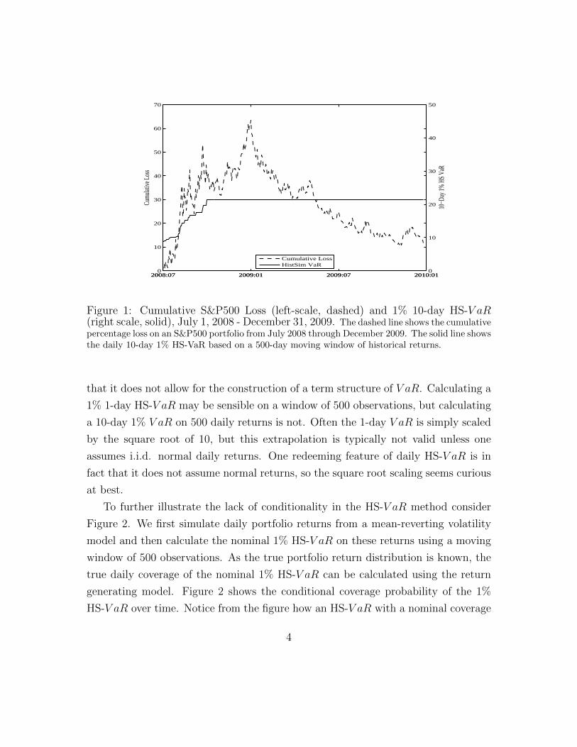
Figure 1 directly illustrates this hidden danger of HS. We plot on the left axis

the cumulative daily loss (cumulative negative return) on an S&P500 portfolio, and

on the right axis the 1% HS-V aR calculated using a 500 day moving window, for a

sample period encompassing the recent financial crisis (July 1, 2008 - December 31,

2009). Notice that HS-V aR reacts only slowly to the dramatically increased risk in

the fall of 2008. Perhaps even more strikingly, HS-V aR reacts very slowly to the

decreased risk following the market trough in March 2009. The 500-day HS-V aR

remains at its peak at the end of 2009. More generally, the sluggishness of HS-

V aR dynamics implies that traders who base their positions on HS will reduce their

exposure too slowly when volatility increases, and then increase exposure too slowly

when volatility subsequently begins to subside.

The sluggish reaction to current market conditions is only one shortcoming of

HS-V aR. Another is the lack of a properly-defined conditional model, which implies

1See also Perignon and Smith (2010a).2Boudoukh et al. (1998) incorporate more aggressive updating into historical simulation, but

the basic concerns expressed by Pritsker (2006) remain.

3

2008:07 2009:01 2009:07 2010:010

10

20

30

40

50

60

70

Cum

ulativ

e Lo

ss

2008:07 2009:01 2009:07 2010:010

10

20

30

40

50

10−D

ay 1

% H

S Va

R

Cumulative LossHistSim VaR

Figure 1: Cumulative S&P500 Loss (left-scale, dashed) and 1% 10-day HS-V aR(right scale, solid), July 1, 2008 - December 31, 2009. The dashed line shows the cumulativepercentage loss on an S&P500 portfolio from July 2008 through December 2009. The solid line showsthe daily 10-day 1% HS-VaR based on a 500-day moving window of historical returns.

that it does not allow for the construction of a term structure of V aR. Calculating a

1% 1-day HS-V aR may be sensible on a window of 500 observations, but calculating

a 10-day 1% V aR on 500 daily returns is not. Often the 1-day V aR is simply scaled

by the square root of 10, but this extrapolation is typically not valid unless one

assumes i.i.d. normal daily returns. One redeeming feature of daily HS-V aR is in

fact that it does not assume normal returns, so the square root scaling seems curious

at best.

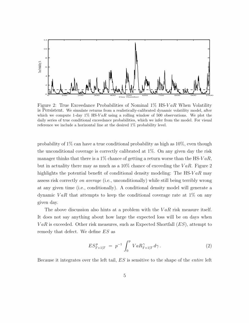
To further illustrate the lack of conditionality in the HS-V aR method consider

Figure 2. We first simulate daily portfolio returns from a mean-reverting volatility

model and then calculate the nominal 1% HS-V aR on these returns using a moving

window of 500 observations. As the true portfolio return distribution is known, the

true daily coverage of the nominal 1% HS-V aR can be calculated using the return

generating model. Figure 2 shows the conditional coverage probability of the 1%

HS-V aR over time. Notice from the figure how an HS-V aR with a nominal coverage

4

0 100 200 300 400 500 600 700 800 900 10000

2

4

6

8

10

12Tru

e Proba

bility, %

Day Number

Figure 2: True Exceedance Probabilities of Nominal 1% HS-V aR When Volatilityis Persistent. We simulate returns from a realistically-calibrated dynamic volatility model, afterwhich we compute 1-day 1% HS-V aR using a rolling window of 500 observations. We plot thedaily series of true conditional exceedance probabilities, which we infer from the model. For visualreference we include a horizontal line at the desired 1% probability level.

probability of 1% can have a true conditional probability as high as 10%, even though

the unconditional coverage is correctly calibrated at 1%. On any given day the risk

manager thinks that there is a 1% chance of getting a return worse than the HS-V aR,

but in actuality there may as much as a 10% chance of exceeding the V aR. Figure 2

highlights the potential benefit of conditional density modeling: The HS-V aR may

assess risk correctly on average (i.e., unconditionally) while still being terribly wrong

at any given time (i.e., conditionally). A conditional density model will generate a

dynamic V aR that attempts to keep the conditional coverage rate at 1% on any

given day.

The above discussion also hints at a problem with the V aR risk measure itself.

It does not say anything about how large the expected loss will be on days when

V aR is exceeded. Other risk measures, such as Expected Shortfall (ES), attempt to

remedy that defect. We define ES as

ES pT+1|T = p−1

∫ p

0

V aR γT+1|T dγ . (2)

Because it integrates over the left tail, ES is sensitive to the shape of the entire left

5

tail of the distribution.3 By averaging all of the V aRs below a prespecified coverage

rate, the magnitude of the loss across all relevant scenarios matters. Thus, even if

the V aR might be correctly calibrated at, say, the 5% level, this does not ensure that

the 5% ES is also correct. Conversely, even if the 5% ES is estimated with precision,

this does not imply that the 5% V aR is valid. Only if the return distribution is

characterized appropriately throughout the entire tail region can we guarantee that

the different risk measures all provide accurate answers.

Our main point of critique still applies, however. Any risk measure, whether V aR,

ES, or anything else, that neglects conditionality, will inevitably miss important

aspects of the dynamic evolution of risk. In the conditional analyses of subsequent

sections, we focus mostly on conditional V aR, but we also treat conditional ES.4

1.3 Plan of the Chapter

We proceed systematically in several steps. In section 2 we consider portfolio level

analysis, directly modeling conditional portfolio volatility using exponential smooth-

ing and GARCH models, along with more recent “realized volatility” procedures that

effectively incorporate the information in high-frequency intraday data.

In section 3 we consider asset level analysis, modeling asset conditional covariance

matrices, again using GARCH and realized volatility techniques. The relevant cross-

sectional dimension is often huge, so we devote special attention to dimensionality-

reduction methods.

In section 4 we consider links between return volatilities and macroeconomic

fundamentals, with special attention to interactions across the business cycle.

We conclude in section 5.

3In contrast to V aR, the expected shortfall is a coherent risk measure in the sense of Artzneret al. (1999) as demonstrated by, e.g., Follmer and Schied (2002). Among other things, this ensuresthat it captures the beneficial effects of portfolio diversification, unlike V aR.

4ES is increasingly used in financial institutions, but it has not been incorporated into theinternational regulatory framework for risk control, likely because it is harder than V aR to estimatereliably in practice.

6

2 Conditional Portfolio-Level Risk Analysis

The portfolio risk measurements that we discuss in this section require only a univari-

ate portfolio-level model. In contrast, active portfolio risk management, including

V aR minimization and sensitivity analysis, as well as system-wide risk measure-

ments, all require a multivariate model, as we discuss subsequently in section 3.

In practice, portfolio level analysis is often done via historical simulation, as

detailed above. We argue, however, that there is no reason why one cannot esti-

mate a parsimonious dynamic model for portfolio level returns. If interest centers

on the distribution of the portfolio returns, then this distribution can be modeled

directly rather than via aggregation based on a larger, and almost inevitably less

well-specified, multivariate model.

The construction of historical returns on the portfolio in place is a necessary

precursor to any portfolio-level risk analysis. In principle it is easy to construct a

time series of historical portfolio returns using current portfolio holdings, WT =

(w1,T , . . . , wN,T )′

and historical asset returns,5 Rt = (r1,t, . . . , rN,t)′:

rw,t =N∑i=1

wi,T ri,t ≡ W′

T Rt, t = 1, 2, ..., T . (3)

In practice, however, historical prices for the assets held today may not be avail-

able. Examples where difficulties arise include derivatives, individual bonds with

various maturities, private equity, new public companies, merger companies and so

on. For these cases “pseudo” historical prices must be constructed using either pric-

ing models, factor models or some ad hoc considerations. The current assets without

historical prices can, for example, be matched to “similar” assets by capitalization,

industry, leverage, and duration. Historical pseudo asset prices and returns can then

be constructed using the historical prices on the substitute assets.

We focus our discussion on V aR.6 We begin with a discussion of the direct com-

5The portfolio return is a linear combination of asset returns when simple rates of returns areused. When log returns are used the portfolio return is only approximately linear in asset returns.

6Although the Basel Accord calls for banks to report 1% V aR’s, for various reasons banks tend

7

putation of portfolio V aR via exponential smoothing, followed by GARCH modeling,

and more recent realized volatility based procedures. Notwithstanding a number of

well-know drawbacks, see, e.g., Stulz (2008), V aR remains by far the most prominent

and commonly-used quantitative risk measure. The main techniques that we discuss

are, however, easily adapted to allow for the calculation of other portfolio-level risk

measures, and we will briefly discuss how to do so as well.

2.1 Modeling Time-Varying Volatilities Using Daily Data

and GARCH

The lack of conditionality in the HS-V aR and related HS approaches discussed above

is a serious concern. Several procedures are available for remedying this deficiency.

Chief among these are RiskMetrics (RM) and Generalized Autoregressive Conditional

Heteroskedasticity (GARCH) models, both of which are easy to implement on a

portfolio basis. We discuss each approach in turn.

2.1.1 Exponential Smoothing and RiskMetrics

Whereas the HS-V aR methodology makes no explicit assumptions about the dis-

tributional model generating the returns, the RM filter/model implicitly assumes

a very tight parametric specification by incorporating conditionality via univariate

portfolio-level exponential smoothing of squared portfolio returns. This directly par-

allels the exponential smoothing of individual return squares and cross products that

underlies the basic RM approach at the individual asset level.7

Again, taking the portfolio-level pseudo returns from (3) as the data series of

to report more conservative V aR’s; see, e.g., the results in Berkowitz and O’Brien (2002), Perignonet al. (2008), Perignon and Smith (2010a) and Perignon and Smith (2010b). Rather than simplyscaling up a 1% V aR based on some “arbitrary” multiplication factor, the procedures that wediscuss below may readily be used to achieve any desired, more conservative, V aR.

7Empirically more realistic long-memory hyperbolic decay structures, similar to the long-memorytype GARCH models briefly discussed below, have also been explored by RM more recently; see,e.g., Zumbach (2006). However, following standard practice we will continue to refer to exponentialsmoothing simply as the RM approach.

8

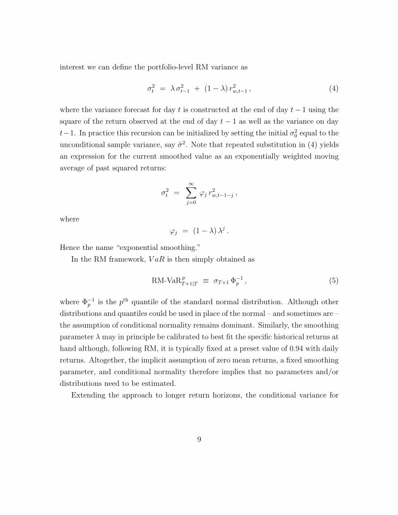
interest we can define the portfolio-level RM variance as

σ2t = λσ2

t−1 + (1− λ) r2w,t−1 , (4)

where the variance forecast for day t is constructed at the end of day t− 1 using the

square of the return observed at the end of day t− 1 as well as the variance on day

t−1. In practice this recursion can be initialized by setting the initial σ20 equal to the

unconditional sample variance, say σ2. Note that repeated substitution in (4) yields

an expression for the current smoothed value as an exponentially weighted moving

average of past squared returns:

σ2t =

∞∑j=0

ϕj r2w,t−1−j ,

where

ϕj = (1− λ)λj .

Hence the name “exponential smoothing.”

In the RM framework, V aR is then simply obtained as

RM-VaR pT+1|T ≡ σT+1 Φ−1

p , (5)

where Φ−1p is the pth quantile of the standard normal distribution. Although other

distributions and quantiles could be used in place of the normal – and sometimes are –

the assumption of conditional normality remains dominant. Similarly, the smoothing

parameter λ may in principle be calibrated to best fit the specific historical returns at

hand although, following RM, it is typically fixed at a preset value of 0.94 with daily

returns. Altogether, the implicit assumption of zero mean returns, a fixed smoothing

parameter, and conditional normality therefore implies that no parameters and/or

distributions need to be estimated.

Extending the approach to longer return horizons, the conditional variance for

9

the k-day return in RM is

V ar(rw,t+k + rw,t+k−1 + ...+ rw,t+1 |Ft) ≡ σ2t:t+k|t = k σ2

t+1 . (6)

Hence the RM model can be thought of as a random walk model in variance, insofar

as the variance scales with the return horizon. More precisely, exponential smoothing

is optimal if and only if squared returns follow a “random walk plus noise” model – a

“local level” model in the terminology of Harvey (1989) – in which case the minimum

MSE forecast at any horizon is simply the current smoothed value.8

Unfortunately, however, the historical record of volatility across numerous asset

classes suggest that volatilities are unlikely to follow random walks, and hence that

the flat forecast function associated with exponential smoothing is inappropriate for

volatility. In particular, the lack of mean-reversion in the RM variance calculations

implies that the term structure of volatility is always flat, which violates both in-

tuition and historical experience. Suppose, for example, that current volatility is

high by historical standards, as was the case during the height of the financial crisis

and the earlier part of the sample in Figures 1 and 2. The RM model will then

simply extrapolate the high current volatility across all future horizons. By contrast,

an empirically more realistic mean-reverting volatility model would correctly predict

that the high volatility observed during the crisis would eventually subside.

The dangers of simply scaling the daily variance by the horizon k, as done in

(6), are discussed further in Diebold et al. (1998a). Of course, the one-day RM

volatility does adjust much more quickly to changing market conditions than the

HS approach, but the flat volatility term structure is unrealistic and, when taken

literally, RM does not appear to be a prudent approach to volatility modeling and

measurement. Furthermore, it is only valid as a volatility filter and not as a data

generating process for simulating future returns. Hence we now turn to GARCH

models, which allow for much richer terms structures of volatility and which can be

used to simulate the return process forward in time.

8See Nerlove and Wage (1964).

10

2.1.2 The GARCH(1,1) Model

To allow for time variation in both the conditional mean and variance of univariate

portfolio returns, we write

rw,t = µt + σt zt , zt ∼ i.i.d. , E(zt) = 0 , V ar(zt) = 1 . (7)

For simplicity we will henceforth assume a zero conditional mean, µt ≡ 0. This

directly parallels the RM approach, and it is a common assumption in risk manage-

ment when short (e.g., daily or weekly) return horizons are considered. It is readily

justified by the fact that the magnitude of the daily volatility (conditional standard

deviation) σt easily dominates that of µt for most portfolios of practical interest. This

is also indirectly manifest by the fact that, in practice, accurate estimation of the

mean is typically much more difficult than accurate estimation of volatility. Still,

conditional mean dynamics could easily be incorporated into any of the GARCH

models discussed below by considering demeaned returns rw,t − µt in place of rw,t.

The key object of interest is the conditional standard deviation, σt. If it depends

non-trivially on the currently observed conditioning information, we say that rw,t

follows a GARCH process. Numerous competing parameterizations for σt have been

proposed in the literature for best capturing the temporal dependencies in the con-

ditional variance of portfolio returns; see, e.g., the list of models and corresponding

acronyms in Bollerslev (2010). However, the simple symmetric GARCH(1,1) intro-

duced by Bollerslev (1986) remains by far the most commonly used formulation in

practice. The GARCH(1,1) model is defined by

σ2t = ω + α r2

w,t−1 + β σ2t−1 . (8)

Extensions to higher order GARCH models are straightforward but usually unnec-

essary empirically, so we concentrate on the GARCH(1,1) throughout most of the

chapter, while discussing some important generalizations in the following section.

Perhaps surprisingly, GARCH is closely-related to exponential smoothing of squared

11

returns. Repeated substitution in (8) yields

σ2t =

ω

1− β+ α

∞∑j=1

βj−1 r2t−j,

so the GARCH(1,1) process implies that current volatility is an exponentially weighted

moving average of past squared returns. Hence GARCH(1,1) volatility measurement

is related to RM volatility measurement.

There are, however, crucial differences between GARCH and RM. First, the

GARCH parameters, and hence ultimately the GARCH volatility, are estimated

using rigorous statistical methods that facilitate probabilistic inference. By contrast,

the parameters used in exponential smoothing are set in an ad hoc fashion. More

specifically, the vector of GARCH parameters, θ = (ω, α, β), is typically estimated

by maximizing the log likelihood function,

lnL(θ; rw,T , ..., rw,1) ∝ −T∑t=1

[ln(σ2t (θ)

)− σ−2

t (θ)r2w,t

]. (9)

This likelihood function is based on the assumption that zt in (7) is i.i.d. N(0, 1).

However, the assumption of conditional normality underlying the (quasi-) likelihood

function in (9) is merely a matter of convenience. If the conditional return distri-

bution is non-normal, the resulting quasi MLE generally still produces consistent

and asymptotically normal, albeit not fully efficient, parameter estimates, see, e.g.,

Bollerslev and Wooldridge (1992). The log-likelihood optimization in (9) can only be

done numerically. However, GARCH models are parsimonious and specified directly

in terms of univariate portfolio returns, so that only a single numerical optimization

is needed.9

Second, and crucially from the vantage point of financial market risk measure-

ment, the covariance stationary GARCH(1,1) process has dynamics that eventually

9This optimization can be performed in a matter of seconds on a standard desktop computerusing standard software such as Excel, as discussed by Christoffersen (2003). For further discussionof inference in GARCH models, see also Andersen et al. (2006a).

12

produce reversion in volatility to a constant long-run value. This enables interesting

and realistic forecasts and contrasts sharply with the RM exponential smoothing

approach in which, as discussed earlier, the term structure of volatility is forced to

be flat. To see the mean reversion that GARCH enables, rewrite the GARCH(1,1)

model in (8) as

σ2t = (1− α− β)σ2 + α r2

w,t−1 + β σ2t−1 , (10)

where σ2 ≡ ω/(1− α − β) denotes the long-run, or unconditional daily variance, or

equivalently as

(σ2t − σ2) = α (r2

w,t−1 − σ2) + β (σ2t−1 − σ2) . (11)

Hence the forecasted deviation of the conditional variance from the long-run vari-

ance is a weighted average of the deviation of the current conditional variance from

the long-run variance, and the deviation of the squared return from the long-run

variance. RM’s exponential smoothing creates a parallel weighted average, with the

key difference that exponential smoothing imposes α + β = 1, whereas covariance

stationary GARCH(1,1) imposes α + β < 1. Finally, we can rearrange (11) to write

(σ2t − σ2) = (α + β) (σ2

t−1 − σ2) + ασ2t−1 (z2

t−1 − 1), (12)

where the last term on the right has zero mean. Hence, the mean reversion of

the conditional variance (or lack thereof) is governed by (α + β). So long as (α +

β) < 1, which must hold for the covariance stationary GARCH(1,1) processes of

empirical relevance, the conditional variance is mean-reverting, with the speed of

mean reversion governed by (α + β).

The mean-reverting property of GARCH volatility forecasts has important impli-

cations for the volatility term structure. To construct the volatility term structure

corresponding to a GARCH(1,1) model, we need the k-day ahead conditional vari-

ance forecast. By repeated substitution in equation (12), we obtain

σ2t+k|t = σ2 + (α + β)k−1 (σ2

t+1 − σ2) . (13)

13

Under our maintained assumption that returns have conditional mean zero, the vari-

ance of the k-day cumulative return is simply the sum of the corresponding 1- through

k-day ahead variance forecasts. Simplifying this sum, it may be informatively ex-

pressed as

σ2t:t+k|t = k σ2 + (σ2

t+1 − σ2)

(1− (α + β)k

1− α− β

). (14)

Hence, in contrast to the flat volatility term structure associated with the RM fore-

cast in (6), the GARCH volatility term structure is upward or downward sloping

depending on the level of current conditional variance compared to long-run vari-

ance.

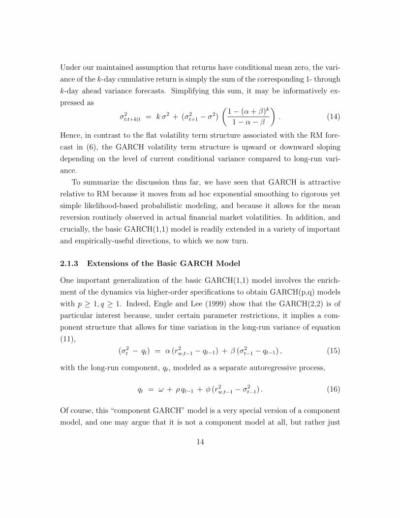
To summarize the discussion thus far, we have seen that GARCH is attractive

relative to RM because it moves from ad hoc exponential smoothing to rigorous yet

simple likelihood-based probabilistic modeling, and because it allows for the mean

reversion routinely observed in actual financial market volatilities. In addition, and

crucially, the basic GARCH(1,1) model is readily extended in a variety of important

and empirically-useful directions, to which we now turn.

2.1.3 Extensions of the Basic GARCH Model

One important generalization of the basic GARCH(1,1) model involves the enrich-

ment of the dynamics via higher-order specifications to obtain GARCH(p,q) models

with p ≥ 1, q ≥ 1. Indeed, Engle and Lee (1999) show that the GARCH(2,2) is of

particular interest because, under certain parameter restrictions, it implies a com-

ponent structure that allows for time variation in the long-run variance of equation

(11),

(σ2t − qt) = α (r2

w,t−1 − qt−1) + β (σ2t−1 − qt−1) , (15)

with the long-run component, qt, modeled as a separate autoregressive process,

qt = ω + ρ qt−1 + φ (r2w,t−1 − σ2

t−1) . (16)

Of course, this “component GARCH” model is a very special version of a component

model, and one may argue that it is not a component model at all, but rather just

14

a restricted GARCH(2,2).

More general component modeling is easily undertaken, however, allowing for

additive superposition of independent autoregressive-type components, as in Gallant

et al. (1999), Alizadeh et al. (2002) and Christoffersen et al. (2008), all of whom

find evidence of component structure in volatility. Under appropriate conditions,

such structures may be shown to approximate very strong dependence, i.e. “long-

memory,” in which shocks to the conditional variance decay at a slow hyperbolic

rate, see, e.g., Granger (1980), Cox (1981), Andersen and Bollerslev (1997), and

Barndorff-Nielsen and Shephard (2001).

Exact long-memory behavior can also easily be incorporated into the GARCH

modeling framework to more closely mimic the dependencies observed with most

financial assets and/or portfolios; see, e.g., Bollerslev and Mikkelsen (1999).10 As

discussed further below, properly incorporating these types of long-memory depen-

dencies generally also results in more accurate volatility forecasts over long horizons.

To take a second example of the extensibility of GARCH models, note that all

of the models considered so far, including the RM filter, imply symmetric response

to positive and negative return shocks. However, equity markets, and particularly

equity indexes, often seem to display a strong asymmetry, whereby a negative return

boosts volatility by more than a positive return of the same absolute magnitude.

The standard GARCH model is readily extended to capture this effect by simply

including a separate term for the past negative return shocks, as in the so-called

threshold-GARCH model proposed by Glosten et al. (1993),

σ2t = ω + α r2

w,t−1 + γ r2w,t−1 I(rw,t−1 < 0) + β σ2

t−1 , (17)

where I(·) denotes the indicator function. For well diversified equity portfolios γ is

typically estimated to be positive and highly statistically significant. In fact, the

asymmetry in the volatility appears to have increased over time and the estimate

10The basic RiskMetrics approach has also recently been extended to allow the smoothing param-eters ϕj used in filtering the returns to exhibit a fixed pre-specified hyperbolic slow long-memorytype decay; see Zumbach (2006). However, the same general set of drawbacks pertaining to thebasic RM filter remain.

15

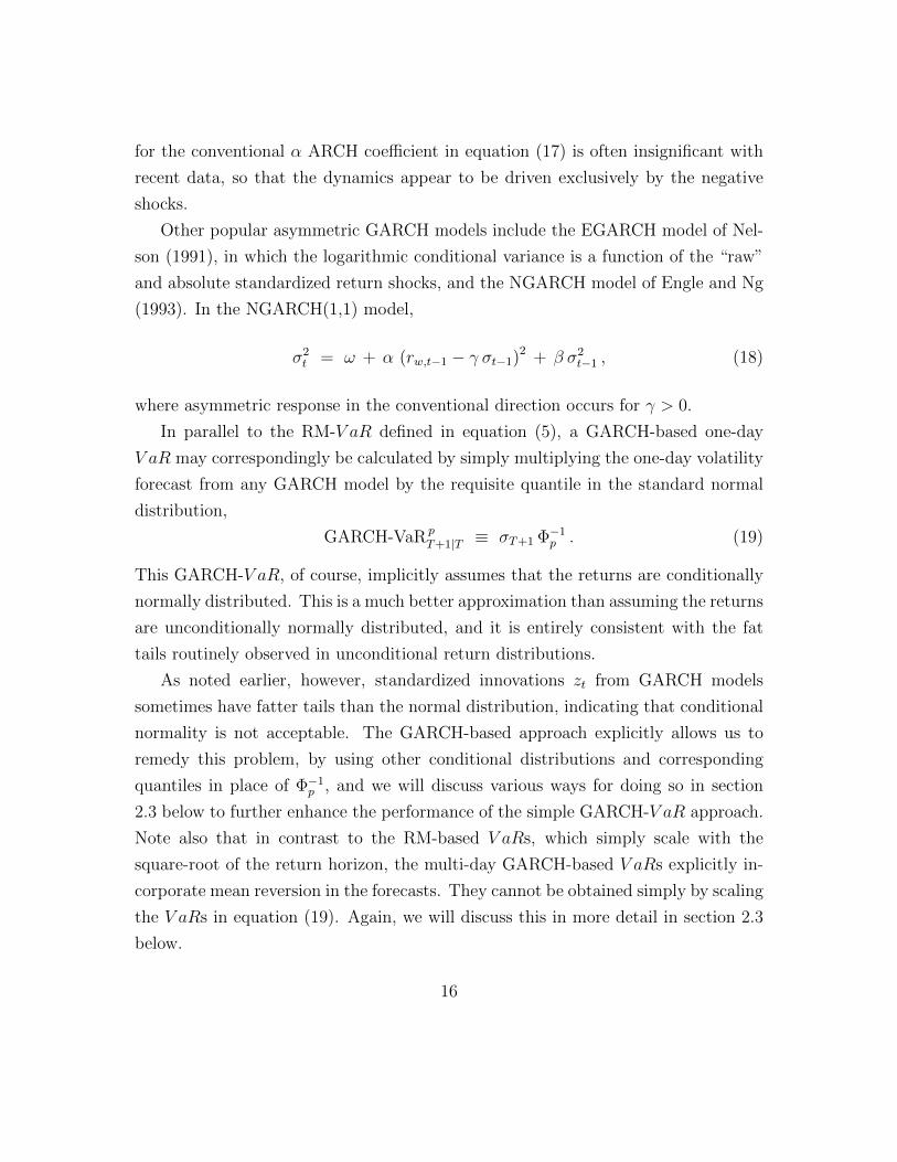
for the conventional α ARCH coefficient in equation (17) is often insignificant with

recent data, so that the dynamics appear to be driven exclusively by the negative

shocks.

Other popular asymmetric GARCH models include the EGARCH model of Nel-

son (1991), in which the logarithmic conditional variance is a function of the “raw”

and absolute standardized return shocks, and the NGARCH model of Engle and Ng

(1993). In the NGARCH(1,1) model,

σ2t = ω + α (rw,t−1 − γ σt−1)2 + β σ2

t−1 , (18)

where asymmetric response in the conventional direction occurs for γ > 0.

In parallel to the RM-V aR defined in equation (5), a GARCH-based one-day

V aR may correspondingly be calculated by simply multiplying the one-day volatility

forecast from any GARCH model by the requisite quantile in the standard normal

distribution,

GARCH-VaR pT+1|T ≡ σT+1 Φ−1

p . (19)

This GARCH-V aR, of course, implicitly assumes that the returns are conditionally

normally distributed. This is a much better approximation than assuming the returns

are unconditionally normally distributed, and it is entirely consistent with the fat

tails routinely observed in unconditional return distributions.

As noted earlier, however, standardized innovations zt from GARCH models

sometimes have fatter tails than the normal distribution, indicating that conditional

normality is not acceptable. The GARCH-based approach explicitly allows us to

remedy this problem, by using other conditional distributions and corresponding

quantiles in place of Φ−1p , and we will discuss various ways for doing so in section

2.3 below to further enhance the performance of the simple GARCH-V aR approach.

Note also that in contrast to the RM-based V aRs, which simply scale with the

square-root of the return horizon, the multi-day GARCH-based V aRs explicitly in-

corporate mean reversion in the forecasts. They cannot be obtained simply by scaling

the V aRs in equation (19). Again, we will discuss this in more detail in section 2.3

below.

16

2008:07 2009:01 2009:07 2010:010

10

20

30

40

50

60

70

Cum

ulat

ive

Loss

2008:07 2009:01 2009:07 2010:010

10

20

30

40

50

10−D

ay 1

% V

aR

Cumulative LossRM−VaRGARCH−VaR

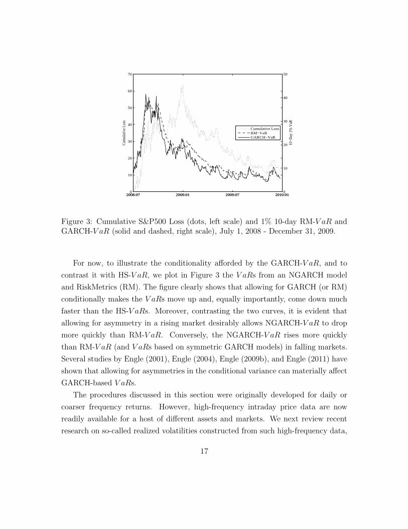
Figure 3: Cumulative S&P500 Loss (dots, left scale) and 1% 10-day RM-V aR andGARCH-V aR (solid and dashed, right scale), July 1, 2008 - December 31, 2009.

For now, to illustrate the conditionality afforded by the GARCH-V aR, and to

contrast it with HS-V aR, we plot in Figure 3 the V aRs from an NGARCH model

and RiskMetrics (RM). The figure clearly shows that allowing for GARCH (or RM)

conditionally makes the V aRs move up and, equally importantly, come down much

faster than the HS-V aRs. Moreover, contrasting the two curves, it is evident that

allowing for asymmetry in a rising market desirably allows NGARCH-V aR to drop

more quickly than RM-V aR. Conversely, the NGARCH-V aR rises more quickly

than RM-V aR (and V aRs based on symmetric GARCH models) in falling markets.

Several studies by Engle (2001), Engle (2004), Engle (2009b), and Engle (2011) have

shown that allowing for asymmetries in the conditional variance can materially affect

GARCH-based V aRs.

The procedures discussed in this section were originally developed for daily or

coarser frequency returns. However, high-frequency intraday price data are now

readily available for a host of different assets and markets. We next review recent

research on so-called realized volatilities constructed from such high-frequency data,

17

and show how to use them to provide even more accurate assessment and modeling

of daily market risks.

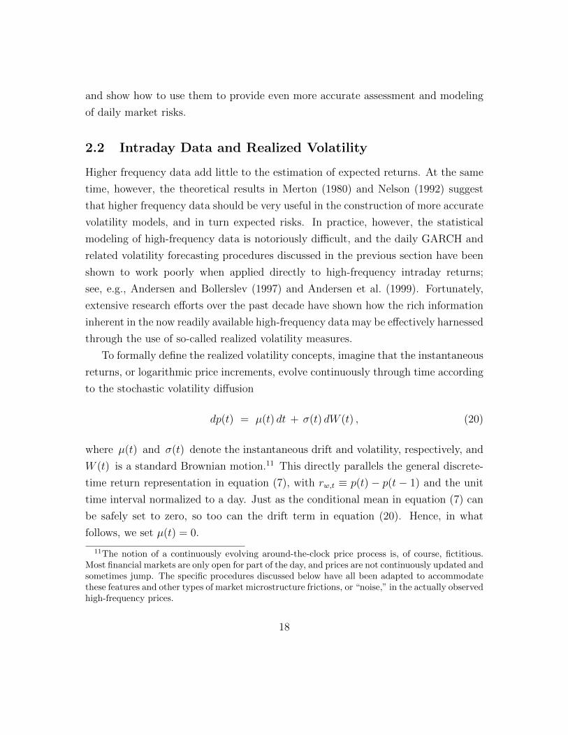
2.2 Intraday Data and Realized Volatility

Higher frequency data add little to the estimation of expected returns. At the same

time, however, the theoretical results in Merton (1980) and Nelson (1992) suggest

that higher frequency data should be very useful in the construction of more accurate

volatility models, and in turn expected risks. In practice, however, the statistical

modeling of high-frequency data is notoriously difficult, and the daily GARCH and

related volatility forecasting procedures discussed in the previous section have been

shown to work poorly when applied directly to high-frequency intraday returns;

see, e.g., Andersen and Bollerslev (1997) and Andersen et al. (1999). Fortunately,

extensive research efforts over the past decade have shown how the rich information

inherent in the now readily available high-frequency data may be effectively harnessed

through the use of so-called realized volatility measures.

To formally define the realized volatility concepts, imagine that the instantaneous

returns, or logarithmic price increments, evolve continuously through time according

to the stochastic volatility diffusion

dp(t) = µ(t) dt + σ(t) dW (t) , (20)

where µ(t) and σ(t) denote the instantaneous drift and volatility, respectively, and

W (t) is a standard Brownian motion.11 This directly parallels the general discrete-

time return representation in equation (7), with rw,t ≡ p(t) − p(t − 1) and the unit

time interval normalized to a day. Just as the conditional mean in equation (7) can

be safely set to zero, so too can the drift term in equation (20). Hence, in what

follows, we set µ(t) = 0.

11The notion of a continuously evolving around-the-clock price process is, of course, fictitious.Most financial markets are only open for part of the day, and prices are not continuously updated andsometimes jump. The specific procedures discussed below have all been adapted to accommodatethese features and other types of market microstructure frictions, or “noise,” in the actually observedhigh-frequency prices.

18

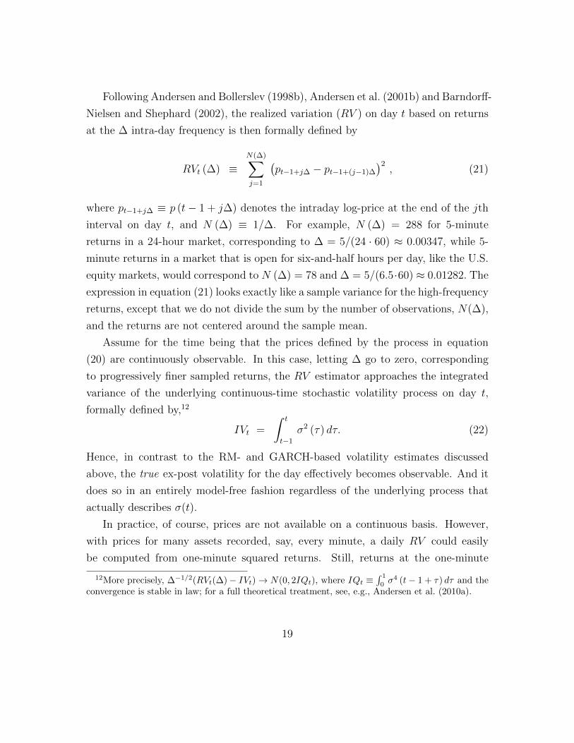
Following Andersen and Bollerslev (1998b), Andersen et al. (2001b) and Barndorff-

Nielsen and Shephard (2002), the realized variation (RV ) on day t based on returns

at the ∆ intra-day frequency is then formally defined by

RVt (∆) ≡N(∆)∑j=1

(pt−1+j∆ − pt−1+(j−1)∆

)2, (21)

where pt−1+j∆ ≡ p (t− 1 + j∆) denotes the intraday log-price at the end of the jth

interval on day t, and N (∆) ≡ 1/∆. For example, N (∆) = 288 for 5-minute

returns in a 24-hour market, corresponding to ∆ = 5/(24 · 60) ≈ 0.00347, while 5-

minute returns in a market that is open for six-and-half hours per day, like the U.S.

equity markets, would correspond to N (∆) = 78 and ∆ = 5/(6.5·60) ≈ 0.01282. The

expression in equation (21) looks exactly like a sample variance for the high-frequency

returns, except that we do not divide the sum by the number of observations, N(∆),

and the returns are not centered around the sample mean.

Assume for the time being that the prices defined by the process in equation

(20) are continuously observable. In this case, letting ∆ go to zero, corresponding

to progressively finer sampled returns, the RV estimator approaches the integrated

variance of the underlying continuous-time stochastic volatility process on day t,

formally defined by,12

IVt =

∫ t

t−1

σ2 (τ) dτ. (22)

Hence, in contrast to the RM- and GARCH-based volatility estimates discussed

above, the true ex-post volatility for the day effectively becomes observable. And it

does so in an entirely model-free fashion regardless of the underlying process that

actually describes σ(t).

In practice, of course, prices are not available on a continuous basis. However,

with prices for many assets recorded, say, every minute, a daily RV could easily

be computed from one-minute squared returns. Still, returns at the one-minute

12More precisely, ∆−1/2(RVt(∆)− IVt)→ N(0, 2IQt), where IQt ≡∫ 1

0σ4 (t− 1 + τ) dτ and the

convergence is stable in law; for a full theoretical treatment, see, e.g., Andersen et al. (2010a).

19

frequency are likely affected by various market microstructure frictions, or noise,

arising from bid-ask bounces, a discrete price grid, and the like.13 Of course, even

with one-minute price observations on hand, we may decide to construct the RV

measures from five-minute returns, as these coarser sampled data are less susceptible

to contamination from market frictions. Clearly, this involves a loss of information

as the majority of the recorded prices are ignored. Expressed differently, it is feasible

to construct five different sets of (overlapping) 5-minute intraday return sequences

from the given data, but in computing the regular five-minute based RV measure we

exploit only one of these series – a theme we return to below.

The optimal choice of high-frequency grid over which to measure the returns

obviously depends on the specific market conditions. The “volatility signature plot”

of Andersen et al. (2000b) is useful for guiding this selection. It often indicates the

adequacy of 5-minute sampling across a variety of assets and markets, as originally

advocated by Andersen and Bollerslev (1998a).14 Meanwhile, as many markets have

become increasingly more liquid it would seem reasonable to resort to even finer

sampling intervals with more recent data although, as noted below, the gains from

doing so in terms of the accuracy of realized volatility based forecast appear to be

fairly minor.

One way to exploit all the high-frequency returns, even if the RV measure is based

on returns sampled at a lower frequency, is to compute alternative RV estimator using

a different offset relative to the first return of the trading day, and then combine

them. For example, if one-minute returns are given, one may construct a new RV

estimator using an equal-weighted average of the five alternative regular five-minute

RV estimators available each day. We will denote this estimator AvgRV below. The

upshot is that the AvgRV estimator based on five-minute returns is much more

robust to microstructure noise than the single RV based on one-minute returns.

In markets that are not open 24 hours per day, the change from the closing price

on day t − 1 to the opening price on day t should also be accounted for. This can

13Brownlees and Gallo (2006) contain a useful discussion of the relevant effects and some of thepractical issues involved in high-frequency data cleaning.

14See also Hansen and Lunde (2006) and the references therein.

20

be done by simply scaling up the trading day RV by the proportion corresponding

to the missing over-night variation, or any of the other more complicated methods

advocated in Hansen and Lunde (2005). As is the case for the daily GARCH mod-

els discussed above, corrections may also be made for the fact that days following

weekends and holidays tend to have proportionally higher than average volatility.

Several other realized volatility estimators have been developed to guard against

the influences of market microstructure frictions. In contrast to the simple RVt(∆)

estimator, which formally deteriorates as the length of the sampling interval ∆ ap-

proaches zero if the prices are observed with error, these other estimators are typ-

ically designed to be consistent for IVt as ∆ → 0, even in the presence of mar-

ket microstructure noise. Especially prominent are the realized kernel estimator of

Barndorff-Nielsen et al. (2008), the pre-averaging estimator of Jacod et al. (2009),

and the two-scale estimator of Aıt-Sahalia et al. (2011). These alternative estimators

are generally more complicated to implement than the AvgRV estimator, requiring

the choice of additional tuning parameters, smoothing kernels, and appropriate block

sizes. Importantly, the results in Andersen et al. (2011a) show that, when used for

volatility forecasting, the simple-to-implement AvgRV estimator performs on par

with, and often better than, these more complex RV estimators.15

To illustrate, we plot in Figure 4 the square root of daily AvgRV s (in annualized

percentage terms) as well as daily S&P 500 returns for January 1, 1990 through

December 31, 2010. Following the discussion above, we construct AvgRV from a

one-minute grid of futures prices and the average of the corresponding five five-

minute RVs.16 Looking at the figure, the assumption of constant volatility is clearly

untenable from a risk management perspective. The dramatic rise in the volatility in

the Fall of 2008 is also immediately evident, with the daily realized volatility reaching

an unprecedented high of 146.2 on October 10, 2008, which is also the day with the

15Note, however, that while the AvgRV estimator provides a very effective way of incorporat-ing ultra high-frequency data into the estimation by averaging all of the possible squared priceincrements over the fixed non-trivial time interval ∆ > 0, the AvgRV estimator is formally notconsistent for IV as ∆→ 0.

16We have one-minute prices from 8:31am to 3:15pm each day. We do not adjust for the overnightreturn.

21

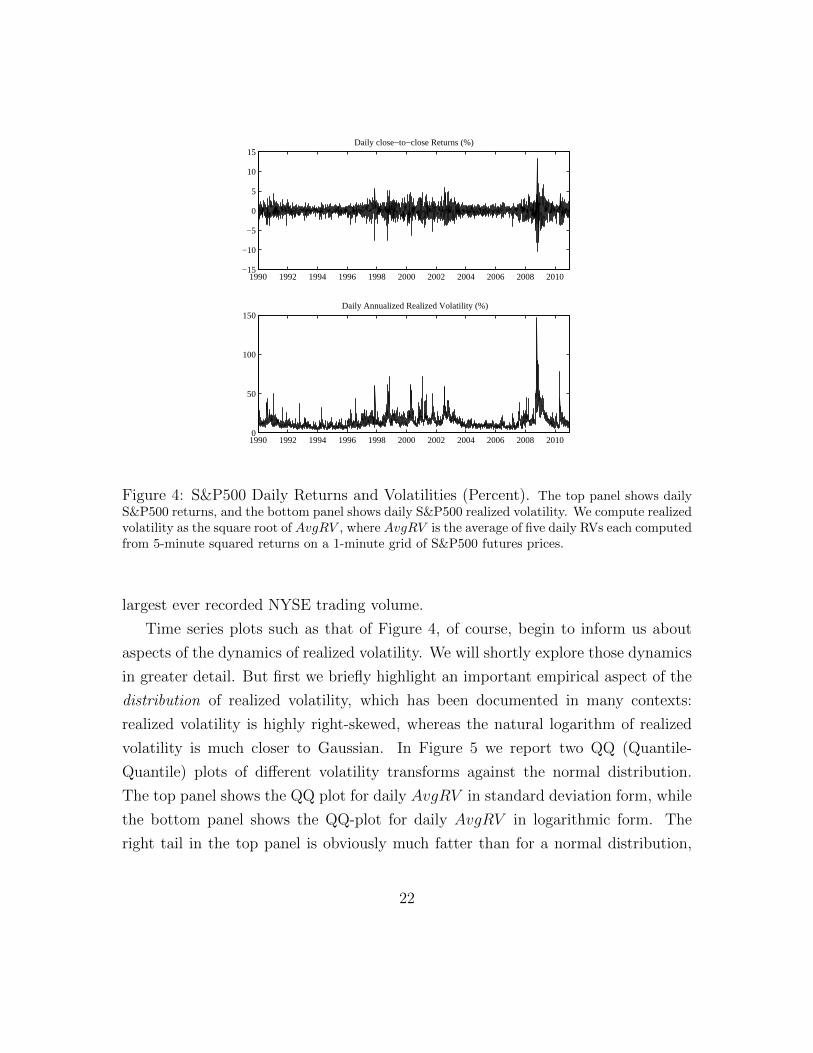
1990 1992 1994 1996 1998 2000 2002 2004 2006 2008 2010−15

−10

−5

0

5

10

15Daily close−to−close Returns (%)

1990 1992 1994 1996 1998 2000 2002 2004 2006 2008 20100

50

100

150Daily Annualized Realized Volatility (%)

Figure 4: S&P500 Daily Returns and Volatilities (Percent). The top panel shows dailyS&P500 returns, and the bottom panel shows daily S&P500 realized volatility. We compute realizedvolatility as the square root of AvgRV , where AvgRV is the average of five daily RVs each computedfrom 5-minute squared returns on a 1-minute grid of S&P500 futures prices.

largest ever recorded NYSE trading volume.

Time series plots such as that of Figure 4, of course, begin to inform us about

aspects of the dynamics of realized volatility. We will shortly explore those dynamics

in greater detail. But first we briefly highlight an important empirical aspect of the

distribution of realized volatility, which has been documented in many contexts:

realized volatility is highly right-skewed, whereas the natural logarithm of realized

volatility is much closer to Gaussian. In Figure 5 we report two QQ (Quantile-

Quantile) plots of different volatility transforms against the normal distribution.

The top panel shows the QQ plot for daily AvgRV in standard deviation form, while

the bottom panel shows the QQ-plot for daily AvgRV in logarithmic form. The

right tail in the top panel is obviously much fatter than for a normal distribution,

22

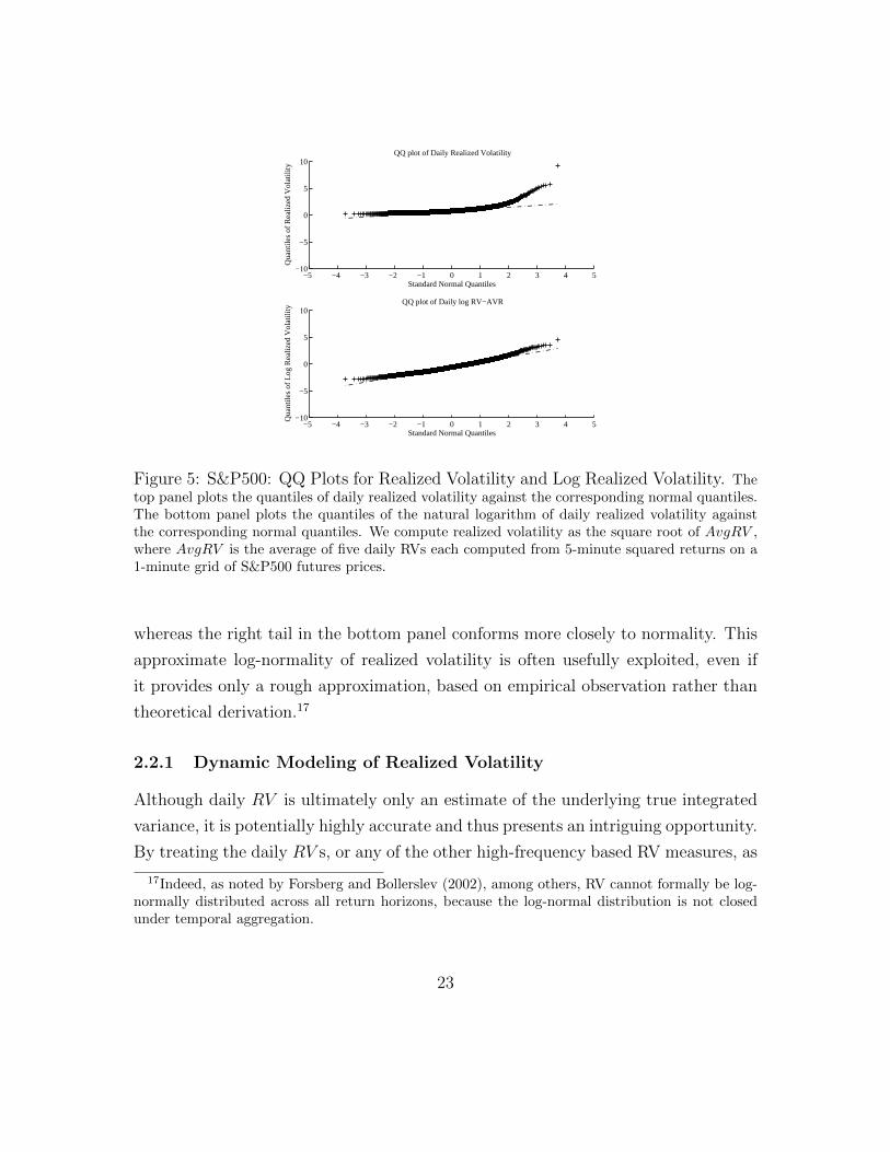
−5 −4 −3 −2 −1 0 1 2 3 4 5−10

−5

0

5

10

Standard Normal QuantilesQ

uant

iles

of R

ealiz

ed V

olat

ility

QQ plot of Daily Realized Volatility

−5 −4 −3 −2 −1 0 1 2 3 4 5−10

−5

0

5

10

Standard Normal Quantiles

Qua

ntile

s of

Log

Rea

lized

Vol

atili

ty QQ plot of Daily log RV−AVR

Figure 5: S&P500: QQ Plots for Realized Volatility and Log Realized Volatility. Thetop panel plots the quantiles of daily realized volatility against the corresponding normal quantiles.The bottom panel plots the quantiles of the natural logarithm of daily realized volatility againstthe corresponding normal quantiles. We compute realized volatility as the square root of AvgRV ,where AvgRV is the average of five daily RVs each computed from 5-minute squared returns on a1-minute grid of S&P500 futures prices.

whereas the right tail in the bottom panel conforms more closely to normality. This

approximate log-normality of realized volatility is often usefully exploited, even if

it provides only a rough approximation, based on empirical observation rather than

theoretical derivation.17

2.2.1 Dynamic Modeling of Realized Volatility

Although daily RV is ultimately only an estimate of the underlying true integrated

variance, it is potentially highly accurate and thus presents an intriguing opportunity.

By treating the daily RV s, or any of the other high-frequency based RV measures, as

17Indeed, as noted by Forsberg and Bollerslev (2002), among others, RV cannot formally be log-normally distributed across all return horizons, because the log-normal distribution is not closedunder temporal aggregation.

23

50 100 150 200 250

0

0.2

0.4

0.6

0.8

Lag Order

Aut

ocor

rela

tion

ACF of Daily RV−AVR

50 100 150 200 250

0

0.2

0.4

0.6

0.8ACF of Daily Return

Lag Order

Aut

ocor

rela

tion

Figure 6: S&P500: Sample Autocorrelations of Daily Realized Variance and DailyReturn. The top panel shows realized variance autocorrelations, and the bottom panel showsreturn autocorrelations, for displacements from 1 through 250 days. Horizontal lines denote 95%Bartlett bands. Realized variance is AvgRV , the average of five daily RVs each computed from5-minute squared returns on a 1-minute grid of S&P500 futures prices.

direct ex-post observations of the true daily integrated variances, the RV approach

permits the construction of ex-ante volatility forecasts using standard ARMA time

series tools. Moreover, recognizing the fact that the measures are not perfect, certain

kinds of measurement errors can easily be incorporated into this framework. The

upshot is that if the frequency of interest is daily, then using sufficiently high-quality

intra-day price data enables the risk manager to treat volatility as effectively ob-

served. This is fundamentally different from the RM filter and GARCH style models

discussed above, in which the daily variances are inferred from past daily returns

conditional on the specific structure of the filter or model.

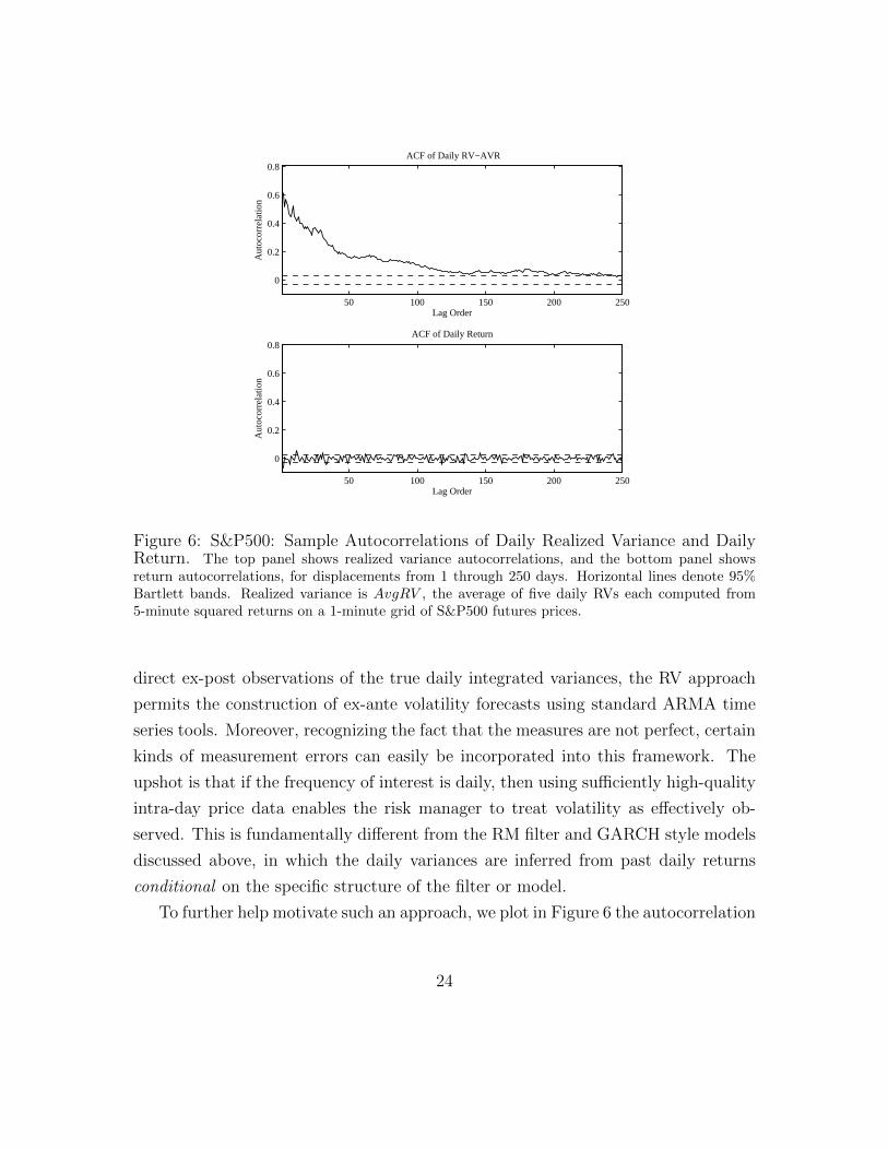
To further help motivate such an approach, we plot in Figure 6 the autocorrelation

24

function (ACF) of daily AvgRV and daily returns. The horizontal lines in each

plot show the Bartlett two-standard-deviation bands around zero. The ACFs are

strikingly different; the realized variance ACF is always positive, highly statistically

significant, and very slowly decaying, whereas the daily return ACF is insignificantly

different from zero. The exceptionally slow decay of the realized variance ACF

suggests long-memory dynamics, in turn implying that equity market volatility is

highly forecastable. This long-memory property of RV is found across numerous asset

classes; see, for example, Andersen et al. (2001b) for evidence on foreign exchange

rates and Andersen et al. (2001a) for comparable results pertaining to individual

equities and equity-index returns.

Simple AR type models provide a natural starting point for capturing these

dependencies. Let RVt denote any of the high-frequency-based realized volatility

measures introduced above. As an example, one could specify a simple first-order

autoregressive model for the daily volatility series,

RVt = β0 + β1RVt−1 + νt . (23)

This, and any higher order AR models for RVt, can easily be estimated by a standard

OLS regression package.

One could go farther and endow integrated variance with AR(1) dynamics, and

recognize that RVt contains some measurement error since in real empirical work the

underlying sampling cannot pass all the way to continuous time. Then RVt would

equal an AR(1) process plus a measurement error, which yields an ARMA(1,1) model

if the two are independent,

RVt = β0 + β1RVt−1 + α1 νt−1 + νt .

Estimation of this model formally requires use of non-linear optimization techniques,

but it is still very easy to do using standard statistical packages.

Although the simple short-memory AR(1) model above may be adequate for

short-horizon risk forecasts, the autocorrelation function for AvgRV shown in Fig-

25

ure 6 clearly suggests that when looking at longer, say monthly, forecast horizons,

more accurate forecasts may be obtained by using richer dynamic models that better

capture the long-range dependence associated with slowly-decaying autocorrelations.

Unfortunately, however, when |β1| < 1 the AR(1) process has short memory, in the

sense that its autocorrelations decay exponentially quickly. On the other hand, when

β1 = 1 the process becomes a random walk (1−L)RVt = β0 +νt, and has such strong

memory that covariance stationarity and mean reversion are both lost. A useful mid-

dle ground may be obtain by allowing for fractional integration,18

(1− L)dRVt = β0 + νt. (24)

This long-memory model is mean reverting if 0 < d < 1 and covariance stationary

if 0 < d < 1/2. Fractional integration contrasts to the extremely strong integer

integration associated with the random walk (d = 1) or the covariance-stationary

AR(1) case (d = 0). Crucially, it allows for long-memory dynamics in the sense that

autocorrelations decay only hyperbolically, akin to the pattern seen in Figure 6.

Long-memory models can, however, be somewhat cumbersome to estimate and

implement. Instead, a simpler approach may be pursued by directly exploiting longer

run realized volatility regressors. Specifically, letting RVt−4:t and RVt−21:t denote the

weekly and monthly realized volatilities, respectively, obtained by summing the cor-

responding daily volatilities. Many researchers, including Andersen et al. (2007a),

have found that the so-called heterogenous autoregressive, or HAR-RV, model, orig-

inally introduced by Corsi (2009),

RVt = β0 + β1RVt−1 + β2RVt−5:t−1 + β3RVt−21:t−1 + νt , (25)

provides a very good fit for most volatility series. As shown in Corsi (2009), the

HAR model may be viewed as an approximate long-memory model. In contrast

to the exact long-memory model above, however, the HAR model can easily be

18The fractional differencing operator (1−L)d is formally defined by its binomial expansion; see,e.g., Baillie et al. (1996) and the discussion therein pertaining to the so-called fractional integratedGARCH (FIGARCH) model.

26

estimated by OLS. Even closer approximations to exact long-memory dependence

can be obtained by including coarser, say quarterly, lagged realized volatilities on

the right-hand side of the equation. A leverage effect, along the lines of the GJR-

GARCH model discussed above, can also easily be incorporated into the HAR-RV

modeling framework by including on the right-hand-side additional volatility terms

interacted with dummies indicating the sign of rt−1, as in Corsi and Reno (2010).

The HAR regressions can, of course, also be written in logarithmic form

logRVt = β0 + β1 logRVt−1 + β2 logRVt−5:t−1 + β3 logRVt−21:t−1 + νt . (26)

The log specification conveniently induces approximate normality, as demonstrated

in Figure 5 above. It also ensures positivity of volatility fits and forecasts, by expo-

nentiating to “undo” the logarithm.19

Armed with a forecast for tomorrow’s volatility from any one of the HAR-RV

or other time series models discussed above, say RV T+1|T , a one-day V aR is easily

computed as

RV − V aR pT+1|T = RV T+1|T Φ−1

p , (27)

where Φ−1p refers to the relevant quantile from the standard normal. Andersen et al.

(2003a) use this observation to construct RV-based V aRs with properties superior to

GARCH-V aR. We will discuss this approach in more detail in section 2.3.2 below.

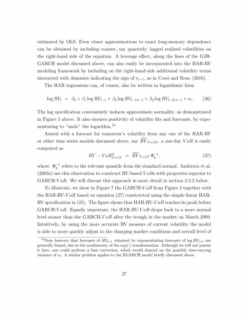
To illustrate, we show in Figure 7 the GARCH-V aR from Figure 3 together with

the HAR-RV-V aR based on equation (27) constructed using the simple linear HAR-

RV specification in (25). The figure shows that HAR-RV-V aR reaches its peak before

GARCH-V aR. Equally important, the HAR-RV-V aR drops back to a more normal

level sooner than the GARCH-V aR after the trough in the market on March 2009.

Intuitively, by using the more accurate RV measure of current volatility the model

is able to more quickly adjust to the changing market conditions and overall level of

19Note however that forecasts of RVt+1 obtained by exponentiating forecasts of logRVt+1 aregenerally biased, due to the nonlinearity of the exp(·) transformation. Although we will not pursueit here, one could perform a bias correction, which would depend on the possibly time-varyingvariance of νt. A similar problem applies to the EGARCH model briefly discussed above.

27

2008:07 2009:01 2009:07 2010:010

5

10

15

20

25

30

35

40

45

50

10−D

ay 1

% V

aR

HAR−VaRGARCH−VaR

Figure 7: 10-day 1% HAR-V aR and GARCH-V aR, July 1, 2008 - December 31,2009. The dashed line shows 10-day 1% HAR-V aR based on the HAR forecasting model for 10-day realized volatility. The solid line shows 10-day 1% GARCH-V aR. When computing V aR the10-day returns divided by the expected volatility are assumed to be normally distributed.

market risk. Of course, the commonly employed RM-V aR in Figure 3 is even slower

to adjust than the GARCH-V aR, and the HS-V aR in Figure 1 adjusts so slowly that

it remains at its maximum sample value at the end of 2009.

As discussed above, V aR and other risk measures are often computed for a two-

week horizon. The risk manager is therefore interested in a 10-day volatility forecast.

Another advantage of the RV based approach, and the HAR-RV model in particular,

is that it can easily be adapted to deliver the required multi-period variance forecasts.

Specifically, consider the modified HAR-RV regression,

RVt:t+9 = β0 + β1RVt−1 + β2RVt−5:t−1 + β3RVt−21:t−1 + νt:t+9 . (28)

An RV based V aR can now easily be computed via

RV − V aRpT+10|T = RV T+1:T+10|T Φ−1

p ,

28

where

RV T+1:T+10|T = β0 + β1RVT + β2RVT−4:T + β3RVT−20:T ,

denotes the 10-day forecast obtained directly from the modified HAR-RV model in

equation (28). Hence, in contrast to GARCH models, there is no need to resort to

the use of complicated recursive expressions along the lines of the formula for σ2t:t+k|t

for the GARCH(1,1) model in equation (14). The modified HAR-RV model in (28)

builds the appropriate mean reversion directly into the requisite variance forecasts.20

2.2.2 Realized Volatilities and Jumps

The continuous-time process in equation (20) formally rules out discontinuities in the

underlying price process. However, financial prices often exhibit “large” movements

over short time-intervals, or “jumps.” A number of these jumps are naturally associ-

ated with readily identifiable macroeconomic news announcement, see, e.g., Andersen

et al. (2003b) and Andersen et al. (2007b), but many others appear idiosyncratic or

asset specific in nature. Such large price moves are inherently more difficult to guard

against, and the measurement and management of jump risk requires the use of dif-

ferent statistical distributions and risk management procedures from the ones needed

to measure and manage the Gaussian diffusive price risks implied by the price process

in equation (20).

In particular, taking into account the possibility of jumps in the underlying price

process, the realized variation measures discussed above no longer converge to the

integrated variance. Instead, the total ex-post variation is given by

QVt = IVt + JVt , (29)

where IVt as before, in equation (22), accounts for the variation coming from the

20Note however that a new HAR-RV model must be estimated for each forecast horizon of interest.

29

continuous, or smooth, price increments over the day, and

JVt =Jt∑j=1

J 2t,j, (30)

measures the variation due to the Jt jumps that occurred on day t; i.e., Jt,j, j =

1, 2, ...,Jt. This does not invalidate AvgRV , or any of the other RV estimators

discussed above, as an ex-post measure for the total daily quadratic variation, or

QVt. It does, however, suggest the use of more refined procedures for separately

estimating QVt and IVt, and in turn JVt.

Several alternative volatility estimators that are (asymptotically) immune to the

impact of jumps have been proposed in the literature. The first was the bipower

variation estimator of Barndorff-Nielsen and Shephard (2004b),

BPVt (∆) =π

2

N (∆)

N (∆)− 1

N(∆)−1∑j=1

|∆pt−1+j∆|∣∣∆pt−1+(j+1)∆

∣∣ , (31)

where ∆pt−1+j∆ ≡ pt−1+j∆ − pt−1+(j−1)∆. The idea behind the bipower variation

estimator is intuitively simple. When ∆ goes to zero the probability of jumps arriving

both in time interval j∆ and (j + 1)∆ goes to zero along with the absolute value of

the non-jump returns. The product |∆pt−1+j∆|∣∣∆pt−1+(j+1)∆

∣∣ will therefore vanish

asymptotically. Consequently, BPVt(∆) will converge to the integrated variance

IVt, as opposed to QVt, for ∆ approaching zero, even in the presence of jumps.21

In contrast, the key terms in the realized variance estimator, namely the intraday

squared returns (∆pt−1+j∆)2, will include the price jumps as well as the “smooth”

continuous price variation. The RVt(∆) estimator therefore always converges to QVt

for ∆ approaching zero.

The BPVt (∆) estimator is subject to the same type of microstructure frictions

that plague the RVt (∆) estimator at ultra-high sampling frequencies. Thus, even

21The π/2 normalization arises from the fact that the expected value of an absolute standardnormal random variable equals (π/2)1/2, while the ratio involving N(∆) provides a finite-sampleadjustment for the loss of one term in the summation.

30

if a one-minute grid of prices is available, it might still be desirable to use coarser,

say five-minute, returns in the calculation of BPVt (∆) to guard against market

microstructure noise. A simple average of the five different BPVt (∆)’s could then

used to compute an improved AvgBPV estimator.

Although the BPVt (∆) estimator is formally consistent for IVt in the idealized

setting without market microstructure noise, the presence of large jumps can result

in non-trivial upward biases in practice. Motivated by this observation, Andersen

et al. (2010c) recently proposed an alternative class of jump-robust estimators, the

neighborhood truncation measures. The simplest version takes the form,

MinRVt (∆) =π

π − 2

(N (∆)

N (∆)− 1

) N(∆)−1∑j=1

min|∆pt−1+j∆| ,

∣∣∆pt−1+(j+1)∆

∣∣2.

The intuition behind the MinRV estimator is similar to that for the original BPV

estimator. When ∆ goes to zero, the probability of jumps arriving in two adjacent

time-intervals of length ∆ goes to zero, so the minimum is unaffected by jumps. The

main difference is that the jump is now fully neutralized, even at a given discrete

sampling frequency, in the sense that the jump size has no direct impact on the

estimator. Hence the finite sample distortion of the MinRV estimator is significantly

less than that of BPV estimator.22 By this same reasoning, a related jump-robust

MedRV estimator may be constructed from the properly scaled square of the median

of three adjacent absolute returns cumulated across the trading day, see Andersen

et al. (2010c) for details.

Another intuitively simple approach for estimating IVt, first explored empirically

by Mancini (2001), is to use truncation, the idea being that the largest price incre-

ments are the ones associated with jumps. Specifically, by only summing the squared

22This is true as long as there are no adjacent jumps at the sampling frequency used. Bothestimators suffer from significant upward biases if adjacent jumps are present. This has led toadditional procedures that enhance the robustness properties even further; see the discussion inAndersen et al. (2011b).

31

return below a certain threshold,

TVt (∆) =

N(∆)∑j=1

∆p2t−1+j∆ I ( ∆pt−1+j∆ < T ) ,

the resulting estimator again consistently estimates only the continuous variation

provided that the threshold T converges to zero at an appropriate rate as ∆ goes

to zero. Since the continuous variation changes over time, and in turn the likely

magnitude of the corresponding continuous price increments, it is also important to

allow the threshold to vary over time, both within and across days. This choice of

time-varying threshold can be somewhat delicate to implement in practice; see, e.g.,

Bollerslev and Todorov (2011b) and the discussion therein.

Regardless of which of these different IVt estimators is used, we obtain an empir-

ically feasible decomposition of the total daily variation into the part associated with

the “small”, or continuous, price moves, and the part associated with the “large,”

and generally more difficult to hedge, price moves, or jumps. Even if the risk man-

ager is not interested in this separation per se, this decomposition can still be very

useful for the construction of improved V aRs and other related risk measures.

In particular, it is often the case that the variation associated with jumps tends

to be much more erratic and less predictable than the variation associated with the

continuous price component. As such, the simple HAR-RV type forecasting models

discussed above may be improved by allowing for different dynamics for the two

different sources of daily variation. Such an approach was first pursued by Andersen

et al. (2007a), who found that the HAR-RV-CJ model,

RVt = β0 + β1 IVt−1 + β2 IVt−5:t−1 + β3 IVt−21:t−1

+ α1 JVt−1 + α2 JVt−5:t−1 + α3 JVt−21:t−1 + νt ,(32)

indeed produces even better RV forecasts than the HAR-RV model in equation (25),

which implicitly restricts the αi and βi coefficients in equation (32) to be identi-

cal. Instead, by allowing for “α effects” and “β effects” in the HAR-RV-CJ model,

we capture the fact that the variation associated with jumps is less persistent and

32

predictable than the continuous variation.

Further refinements allowing for leverage effects and/or other asymmetries and

non-linearities could easily be incorporated into the same HAR-RV modeling frame-

work by including additional explanatory variables on the right-hand-side. But the

simple-to-estimate HAR-RV-CJ model typically does a remarkably good job of ef-

fectively incorporating the empirically most relevant dynamic dependencies of the

intraday price data into the daily and longer-run volatility forecasts of practical

interest.

2.2.3 Combining GARCH and RV

So far we have presented GARCH and RV based procedures as two distinct ap-

proaches. There are, however, good reasons to combine the two. The ability of RV

to rapidly deliver precise information regarding the current level of volatility along

with the ability of GARCH to appropriately smooth noisy volatility proxies make

such a combination appealing. Another advantage of combined models is the ability

to integrate the RV process naturally within a complete characterization of the return

distribution, thus allowing the RV dynamics to become a natural and direct deter-

minant of the time-variation in risk measures such as V aR and expected shortfall.

The following section will elaborate on those features of the approach.

The simplest way of cobining GARCH and RV is to include the RV measure as

an additional explanatory variable on the right-hand-side of the GARCH equation,

σ2t = ω + α r2

w,t−1 + β σ 2t−1 + γ RVt−1 . (33)

This is often referred to as a GARCH-X model.23 Estimating this model typically re-

sults in a statistically insignificant α (ARCH) coefficient, so that the model effectively

reduces to

σ2t = ω + β σ 2

t−1 + γ RVt−1 . (34)

23Professor Robert F. Engle in his discussion of Andersen et al. (2003a) at the 2000 WesternFinance Association meeting in Sun Valley, Idaho, was among the first to empirically explore thisidea. Related analysis appears in Engle (2002b). Lu (2005) provides another early comprehensiveempirical study of GARCH-X type models.

33

Intuitively, the high-frequency-based RV measure affords a superior estimate of the

true ex-post daily variation compared to the daily (de-meaned) squared returns, in

turn driving out the latter as an explanatory variable for tomorrow’s volatility. As

such, whenever high-frequency based RV measures are available, it is always a good

idea to use the GARCH-X model instead of the conventional GARCH(1,1) model

based solely on daily return observations.24

The GARCH-X model defined by equations (7) and (33) or (34) directly provides

one-day volatility forecasts. The calculation of longer-run k-day forecasts σ2t+k|t ne-

cessitates a model for forecasting RVt+k as well. This could be accomplished in an ad

hoc fashion by simply augmenting the GARCH-X model with any one of the HAR-RV

type models discussed in the previous sections. The so-called Realized GARCH class

of models developed by Hansen et al. (2010a) provides a more systematic approach

for doing exactly that.

As an example, consider the specific Realized GARCH model defined by equation

(7) and

σ2t = ω + β σ 2

t−1 + γRVt−1, (35)

RVt = ωX + βX σ2t + τ (zt) + νt , (36)

where νt denotes a random error with the property that Et(νt) = 0, and the τ (zt)

function allows for a contemporaneous leverage effect via the return shock zt in equa-

tion (7).25 Substituting the equation for σ2t into the equation for RVt shows that the

model implies an ARMA representation for the realized volatility, but other HAR-

RV type structures could, of course, be used instead. Note also that unlike regular

GARCH, the Realized GARCH model has two separate innovations. However, be-

24In a related context, Visser (2011) has recently shown how the accuracy of the coefficientestimates in conventional daily GARCH models may be improved through the use of intradayRV-based measures in the estimation.

25A closely related class of two-shock Realized GARCH models, in which the return volatility is aweighted average of the GARCH and RV volatilities, has recently been proposed by Christoffersenet al. (2011b). Their affine formulation has the advantage that option valuation can be donevia Fourier inversion of the conditional characteristic function. Non-affine approaches to optionvaluation using RV have also been pursued by Corsi et al. (2011) and Stentoft (2008).

34

cause RVt is observed, estimation of the model can still be done using bivariate max-

imum likelihood estimation techniques that closely mirror the easily-implemented

procedures available for regular GARCH models.

The Multiplicative Error Model (MEM) of Engle (2002b) and Engle and Gallo

(2006) constitutes another framework for combining different volatility proxies (e.g.,

daily absolute returns, daily high-low ranges, RVs, IVs, or option implied volatilities)

into the estimation of a coherent multivariate model for return variances.26 It is

natural to use this same framework to extend the GARCH-X model to allow for the

construction of multi-day volatility forecasts.

In particular, building on the MEM structure, Shephard and Sheppard (2010)

propose an extension of the basic GARCH-X model in equation (33), in which the

conditional mean of realized volatility, µRV,t ≡ Et−1(RVt ), is defined recursively by

the equation,

µRV,t = ωRV + αRV RVt−1 + βRV µRV,t−1 . (37)

Shephard and Sheppard (2010) refer to this model as a High-frEquency bAsed Volatil-

itY model, or “HEAVY” model. Like the Realized GARCH class of models, HEAVY

models have the advantage that they adapt to new information and market con-

ditions much more quickly than the regular daily GARCH models. In contrast to

the simple GARCH(1,1) model, for which the k-period variance forecasts in equa-

tion (13) converge monotonically to their long-run run average values, the HEAVY

model defined by equations (33) and (37) also might show momentum effects, so that

the convergence of the multi-period variance forecasts to the long-run unconditional

variance is not necessarily monotonic. This point is nicely illustrated by the volatil-

ity forecasts during the recent financial crises reported in Shephard and Sheppard

(2010), which show how the model sometimes predicts rising volatility even when

the current volatility is exceptionally high by historical standards.

Risk managers, of course, typically do not care directly about the dynamics of

volatility but rather about the dynamics of the entire conditional distribution of

26This approach has also been used by Brownlees and Gallo (2011) to compare different volatilitymeasures and their uses in risk management.

35

portfolio returns. Movement in conditional variance is a key driver of movement in

the conditional distribution, but only in the unlikely case of conditional normality is

it the entire story. Hence we next discuss how GARCH and realized variance may

be used in broader modeling of entire return distributions.

2.3 Modeling Return Distributions

We have emphasized – and continue to emphasize – the potentially seriously mislead-

ing nature of unconditional risk analyses. Here we stress the similarly potentially

seriously misleading nature of Gaussian risk analyses. There are four cases to con-

sider, corresponding to the reliance on unconditional/conditional information and

the use of Gaussian/non-Gaussian distributions.

Risk measurement in an unconditional Gaussian framework would be doubly

defective, first because of the deficiencies of the unconditional perspective, and second

because financial returns are simply not unconditionally Gaussian, as has been well-

known at least since the classic contributions of Mandelbrot (1963) and Fama (1965).

For that reason, even crude approaches like historical HS-VaR, although maintaining

an unconditional perspective, dispense with normality by building an approximation

to the unconditional distribution from historically-observed returns.

Figure 8 serves to illustrate the strong unconditional non-normality in returns,

as it displays a QQ plot for daily S&P500 returns from January 2, 1990 to December

31, 2010. That is, it plots quantiles of the standardized returns against quantiles

of the standard normal distribution. If the returns were unconditionally normally

distributed, the points would fall along the 45-degree line. Clearly, the daily returns

are not normally distributed.

Now consider the conditional case. Note that in specifying the general condi-

tional variance model (7) we made no assumptions as to the conditional distribution

of returns. That is, we made no assumptions as to the distribution of returns stan-

dardized by their conditional variance; i.e., the distribution of zt in equation (7).

But in converting objects like GARCH conditional variances into GARCH-VaR, for

example, we did invoke conditional normality. At least four points are worth making.

36

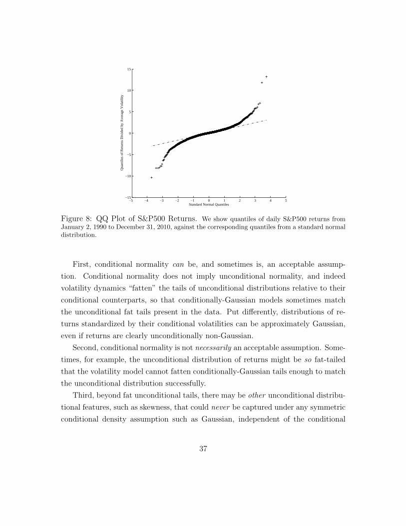
−5 −4 −3 −2 −1 0 1 2 3 4 5−15

−10

−5

0

5

10

15

Standard Normal Quantiles

Qua

ntile

s of

Ret

urns

Div

ided

by

Ave

rage

Vol

atili

ty

Figure 8: QQ Plot of S&P500 Returns. We show quantiles of daily S&P500 returns fromJanuary 2, 1990 to December 31, 2010, against the corresponding quantiles from a standard normaldistribution.

First, conditional normality can be, and sometimes is, an acceptable assump-

tion. Conditional normality does not imply unconditional normality, and indeed

volatility dynamics “fatten” the tails of unconditional distributions relative to their

conditional counterparts, so that conditionally-Gaussian models sometimes match

the unconditional fat tails present in the data. Put differently, distributions of re-

turns standardized by their conditional volatilities can be approximately Gaussian,

even if returns are clearly unconditionally non-Gaussian.

Second, conditional normality is not necessarily an acceptable assumption. Some-

times, for example, the unconditional distribution of returns might be so fat-tailed

that the volatility model cannot fatten conditionally-Gaussian tails enough to match

the unconditional distribution successfully.

Third, beyond fat unconditional tails, there may be other unconditional distribu-

tional features, such as skewness, that could never be captured under any symmetric

conditional density assumption such as Gaussian, independent of the conditional

37

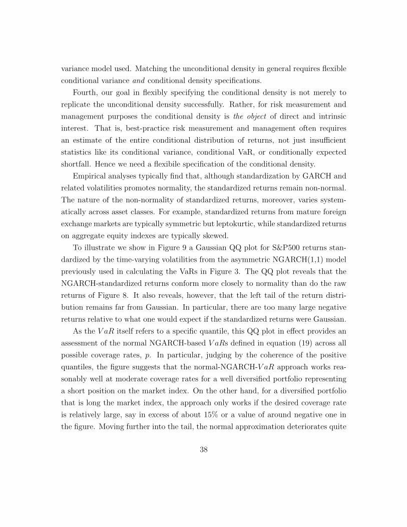
variance model used. Matching the unconditional density in general requires flexible

conditional variance and conditional density specifications.

Fourth, our goal in flexibly specifying the conditional density is not merely to

replicate the unconditional density successfully. Rather, for risk measurement and

management purposes the conditional density is the object of direct and intrinsic

interest. That is, best-practice risk measurement and management often requires

an estimate of the entire conditional distribution of returns, not just insufficient

statistics like its conditional variance, conditional VaR, or conditionally expected

shortfall. Hence we need a flexibile specification of the conditional density.

Empirical analyses typically find that, although standardization by GARCH and

related volatilities promotes normality, the standardized returns remain non-normal.

The nature of the non-normality of standardized returns, moreover, varies system-

atically across asset classes. For example, standardized returns from mature foreign

exchange markets are typically symmetric but leptokurtic, while standardized returns

on aggregate equity indexes are typically skewed.

To illustrate we show in Figure 9 a Gaussian QQ plot for S&P500 returns stan-

dardized by the time-varying volatilities from the asymmetric NGARCH(1,1) model

previously used in calculating the VaRs in Figure 3. The QQ plot reveals that the

NGARCH-standardized returns conform more closely to normality than do the raw

returns of Figure 8. It also reveals, however, that the left tail of the return distri-

bution remains far from Gaussian. In particular, there are too many large negative

returns relative to what one would expect if the standardized returns were Gaussian.

As the V aR itself refers to a specific quantile, this QQ plot in effect provides an

assessment of the normal NGARCH-based V aRs defined in equation (19) across all

possible coverage rates, p. In particular, judging by the coherence of the positive

quantiles, the figure suggests that the normal-NGARCH-V aR approach works rea-

sonably well at moderate coverage rates for a well diversified portfolio representing

a short position on the market index. On the other hand, for a diversified portfolio

that is long the market index, the approach only works if the desired coverage rate

is relatively large, say in excess of about 15% or a value of around negative one in

the figure. Moving further into the tail, the normal approximation deteriorates quite

38

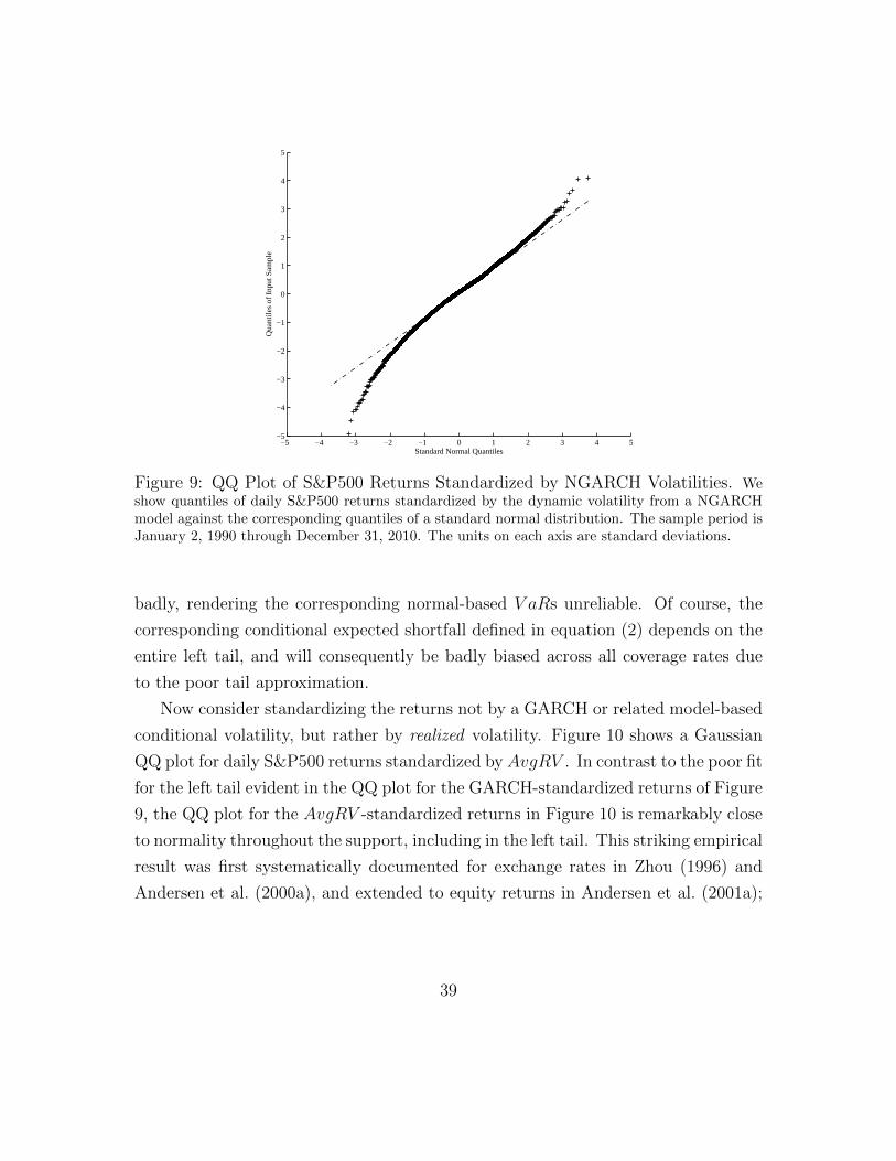
−5 −4 −3 −2 −1 0 1 2 3 4 5−5

−4

−3

−2

−1

0

1

2

3

4

5

Standard Normal Quantiles

Qua

ntile

s of

Inpu

t Sam

ple

Figure 9: QQ Plot of S&P500 Returns Standardized by NGARCH Volatilities. Weshow quantiles of daily S&P500 returns standardized by the dynamic volatility from a NGARCHmodel against the corresponding quantiles of a standard normal distribution. The sample period isJanuary 2, 1990 through December 31, 2010. The units on each axis are standard deviations.

badly, rendering the corresponding normal-based V aRs unreliable. Of course, the

corresponding conditional expected shortfall defined in equation (2) depends on the

entire left tail, and will consequently be badly biased across all coverage rates due

to the poor tail approximation.

Now consider standardizing the returns not by a GARCH or related model-based

conditional volatility, but rather by realized volatility. Figure 10 shows a Gaussian

QQ plot for daily S&P500 returns standardized by AvgRV . In contrast to the poor fit

for the left tail evident in the QQ plot for the GARCH-standardized returns of Figure

9, the QQ plot for the AvgRV -standardized returns in Figure 10 is remarkably close

to normality throughout the support, including in the left tail. This striking empirical

result was first systematically documented for exchange rates in Zhou (1996) and

Andersen et al. (2000a), and extended to equity returns in Andersen et al. (2001a);

39

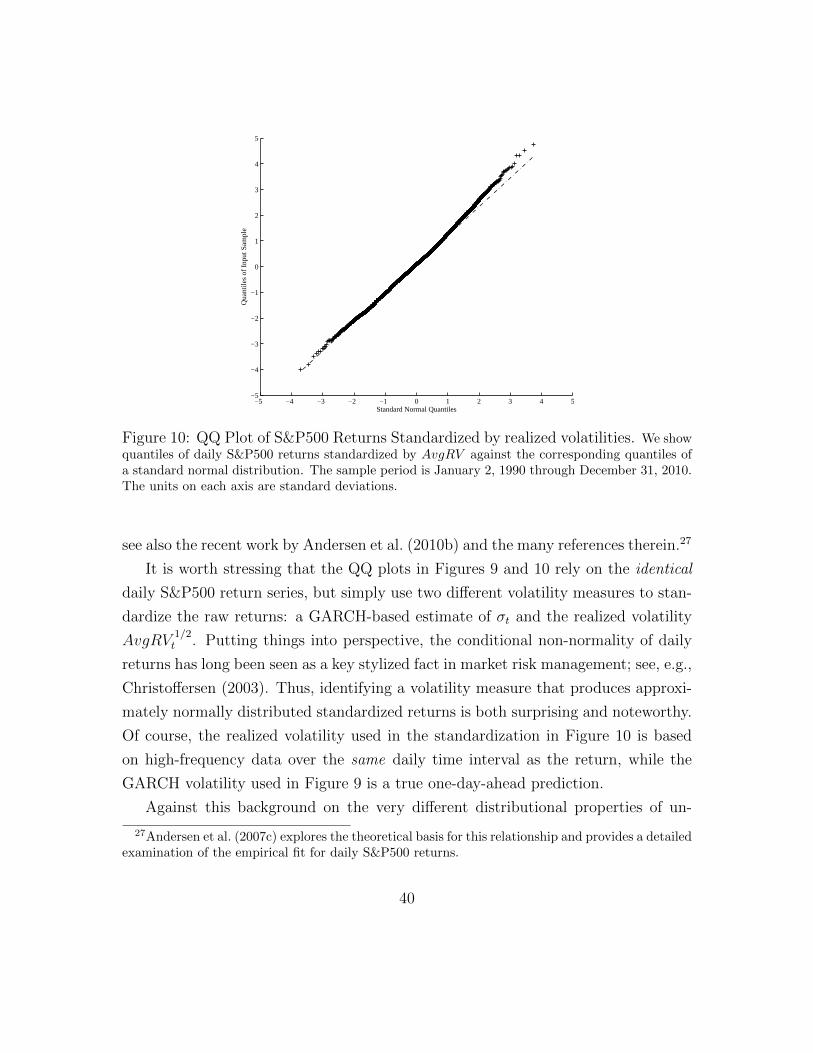
−5 −4 −3 −2 −1 0 1 2 3 4 5−5

−4

−3

−2

−1

0

1

2

3

4

5

Standard Normal Quantiles

Qua

ntile

s of

Inpu

t Sam

ple

Figure 10: QQ Plot of S&P500 Returns Standardized by realized volatilities. We showquantiles of daily S&P500 returns standardized by AvgRV against the corresponding quantiles ofa standard normal distribution. The sample period is January 2, 1990 through December 31, 2010.The units on each axis are standard deviations.

see also the recent work by Andersen et al. (2010b) and the many references therein.27

It is worth stressing that the QQ plots in Figures 9 and 10 rely on the identical

daily S&P500 return series, but simply use two different volatility measures to stan-

dardize the raw returns: a GARCH-based estimate of σt and the realized volatility

AvgRV1/2t . Putting things into perspective, the conditional non-normality of daily

returns has long been seen as a key stylized fact in market risk management; see, e.g.,

Christoffersen (2003). Thus, identifying a volatility measure that produces approxi-

mately normally distributed standardized returns is both surprising and noteworthy.

Of course, the realized volatility used in the standardization in Figure 10 is based

on high-frequency data over the same daily time interval as the return, while the

GARCH volatility used in Figure 9 is a true one-day-ahead prediction.

Against this background on the very different distributional properties of un-

27Andersen et al. (2007c) explores the theoretical basis for this relationship and provides a detailedexamination of the empirical fit for daily S&P500 returns.

40

standardized, GARCH-standardized and RV-standardized returns, in this section we

discuss how to use the different standardizations and resulting distributions to con-

struct accurate predictive return distributions. An important part of that discussion,

particularly in the GARCH-standardized case, involves specification of empirically-

realistic (i.e., non-Gaussian) conditional return distributions.

2.3.1 Procedures Based on GARCH

The GARCH dynamic directly delivers one-day ahead volatility forecasts. In order

to complete the daily predictive return distribution, one simply needs to postulate a

distribution for the zt return shock in equation (7). Although the normal assumption

may work well in certain cases, as Figure 9 makes clear, it often underestimates large

downside risks. As such, it is important to consider alternatives that allow for fat

tails and/or asymmetries in the conditional distribution. Specifically, in the case of

V aR we are looking for ways to more accurately assess the cut-off κ−1p in

V aR pT+1|T ≡ σT+1 κ

−1p , (38)

instead of simply relying on Φ−1p from the standard normal distribution.28 Of course,

doing this for all values of p ∈ [0, 1] essentially amounts to mapping out the entire

conditional return distribution.

Perhaps the most obvious approach is to look for a parametric distribution that is

more flexible than the normal. One example is the (standardized) Student-t distribu-

tion, which relies on only one additional degrees-of-freedom parameter in generating

symmetric fat tails. Such an approach was first pursued by Bollerslev (1987), who

showed how the likelihood function for the normal-GARCH model in equation (9)

is readily extended to the GARCH-t case, thus allowing for the estimation of the

degrees-of-freedom parameter (along with the other GARCH parameters) that best

describes the return distribution, and in turn the requisite κ−1p for calculating the

28The 1996 amendment to the 1988 Basel Accord somewhat arbitrarily recommends the use of amultiplicative factor of at least −3.0 in the construction of a 1% V aR, relative to the Φ−10.01 = −2.33implied by the standard normal distribution; see also the discussion in Chan et al. (2007).

41

V aR in equation (38).

This approach works reasonably well when the conditional return distribution is

close to symmetric. However, as illustrated by the QQ plots discussed above, equity

portfolios are often severely left skewed. The Generalized Error Distribution (GED),

first employed in this context by Nelson (1991), explicitly allows for asymmetries, as

do some of the different generalizations of the Student-t distribution suggested by

Hansen (1994) and Fernandez and Steel (1998), among others. Alternatively, follow-

ing Engle and Gonzalez-Rivera (1991) the whole density for zt may be approximated

using more flexible semiparametric procedures.

Rather than postulating a particular parametric density, one can also simply

approximate the quantiles of non-normal distributions via Cornish-Fisher type ex-

pansions. This approach was first advocated in the context of GARCH modeling

and forecasting by Baillie and Bollerslev (1992). The only inputs needed for esti-

mating κ−1p are the unconditional sample skewness and kurtosis statistics for the

standardized returns.29

Meanwhile, a common problem with most GARCH models, regardless of the

innovation distribution, is that the specific distribution is not preserved under tem-

poral aggregation; see, e.g., the discussion in Drost and Nijman (1993) and Meddahi

and Renault (2004). For example, even if the standardized daily returns from a

GARCH(1,1) model were normal, the implied weekly returns would not be. In turn,

this implies that the term structure of V aRs is not closed under temporal aggrega-

tion either. Instead, the multi-period V aRs need to be computed via Monte Carlo

simulations or other numerical methods, as exemplified by Guidolin and Timmer-

mann (2006).30 This also means that the Cornish-Fisher and related approxima-

tions, which only provide partial characterizations of the underlying daily return

distribution in the form of specific quantiles, generally will not suffice for answer-

29More accurate approximations may in theory be obtained by including higher order uncondi-tional sample moments in the Cornish-Fisher expansion, but this does not always produce satisfac-tory results.

30The affine GARCH models suggested by Heston and Nandi (2000) and Christoffersen et al.(2006), when combined with the methods of Albanese et al. (2004), also allow for relatively easy-to-compute term structures for VaR, but some numerical calculations are still required.

42

ing questions regarding the distribution of temporally aggregated returns. Below,

we discuss a viable approach that effectively combines a parametric volatility model

with a data-driven conditional distribution. First, however, we discuss how realized

volatilities, if available, may be used in the calculation of even more accurate predic-

tive return distributions by effectively incorporating the intraday information into

the distributional forecasts.

2.3.2 Procedures Based on Realized Volatility

The basic idea underlying the construction of RV-based predictive return distri-

butions is to treat the time series of RVs as stochastic. Hence, in contrast to the

GARCH-based procedures, which seek to describe the predictive distribution through

an appropriately specified univariate distribution for the standardized returns, the

RV-based procedures necessitate, at a minimum, a bivariate random distribution for

the returns and the realized volatilities.

This relatively new approach to risk measurement was first suggested by Ander-

sen et al. (2003a). The approach is directly motivated by the empirical regularities

pertaining to the RV measures highlighted above. First, as discussed in section 2.2,

simple time series models for the realized volatilities, like the HAR-RV specifica-

tion, generally result in more accurate volatility forecasts than do the conventional

GARCH models based on daily data only.31 Second, as shown in section 2.3, the

distributions of daily returns standardized by the same-day RVs typically appear

close to Gaussian. Taken together, this suggests a mixture-of-distributions type ap-

proach for characterizing the time T + 1 return distribution, in which the predictive

distribution for RVT+1 serves as the mixture variable.32

Specifically, assuming that the standardized return is normal, rT+1/RV1/2T+1 ∼

N(0, 1), and that the distribution of the time T + 1 realized volatility conditional on

31This empirical regularity may also be justified through more formal theoretical arguments, as towhy the simple reduced form RV-based procedures often work better than structural model-basedapproaches in practice; see, Andersen et al. (2004), Andersen et al. (2011a), and Sizova (2011).

32There is a long history, dating back to Clark (1973), of using mixture-of-distributions to describethe unconditional distribution of returns. What is fundamentally different in the RV-based approachis to treat the mixing variable as directly observable and predictable.

43

time T information is log-normal, the resulting normal log-normal mixture distribu-

tion for the time T + 1 returns may be expressed as

fT (rT+1) =1

2πσ 2`,T+1

∫ ∞0

y−3/2 exp

−r2T+1

2y− 1

2σ 2`,T+1

(ln (y)− µ`,T+1)2

dy ,

where µ`,T+1 and σ 2`,T+1 denote, respectively, the time T conditional mean and vari-

ance of log(RVT+1). For example, postulating a HAR-RV type model for logRV with

homoskedastic errors, we obtain,

µ`,T+1 = β0 + β1 log(RVT ) + β2 log(RVT−4:T ) + β2 log(RVT−20:T ) ,

and σ 2`,T+1 = σ 2

v , respectively.33

The simple HAR-RV model for the conditional mean µ`,T+1 could, of course, be

extended in several directions. For instance, as noted above, when modeling large

equity portfolios, asymmetries, or “leverage effcts,” are often statistically significant.

Also, in their actual empirical implementation Andersen et al. (2003a) use a long-

memory ARFIMA model for logRV in place of the HAR-RV formulation. This

makes little difference for the maximum ten-days forecast horizons considered in

their analysis, but it could be important to do so in the calculation of longer run, say

quarterly (∼ 66 days ahead) or annual (∼ 252 days ahead), distributional forecasts.

The mixture distribution described above treats σ`,t as constant. However, it

is natural to think about the volatility-of-volatility as being time varying with its

own GARCH dynamics. Such an approach has been pursued empirically by Ma-

heu and McCurdy (2011), who report that allowing for temporal variation in σ`,t

does not actually result in materially different predictive return distributions. Go-

ing one step further, Bollerslev et al. (2009a) develop a joint conditional density

model for the returns, the “smooth” volatility, and the variation due to jumps

rt, ln (BPVt) , ln (RVt/BPVt). In that model the predictive distribution for the

33Although it is not possible to express the density function in closed form, it is easy to calculatenumerically by repeated simulations from a normal distribution with a random variance drawn froma log-normal distribution with the requisite mean and variance.

44

returns is therefore obtained through a more complicated normal mixture involving

two separate mixing variables, but the basic idea remains the same.

This continues to be an active area of research, and it is too early to say which of

the different approaches will be the “winner.” It is evident, however, that any of the

relatively simple RV-based procedures described above almost invariably generate

more accurate predictive return distributions than the traditional GARCH-based

distributional forecast, especially over relatively short one-day to one-week horizons.

2.3.3 Combining GARCH and RV

Just as the GARCH and RV concepts may be formally combined in the construction

of volatility forecasts, they may be similarly combined to produce distributional

forecasts. The procedures discussed in the previous section, of course, also utilize

the realized volatility measures in the construction of the forecasts. However, they

generally do not provide a direct link between the GARCH conditional variance σt

and the realized volatility measures.

Forsberg and Bollerslev (2002) provides a first attempt at doing that. Their RV-

GARCH style model is based on the assumption that RV is conditionally Inverse

Gaussian distributed34

fT (RVT+1) ∼ IG(σ 2T+1, η

),

together with a GARCH-style process for the conditional expectation of RV,

ET (RVT+1) = σ 2T+1 = ω + αr2

w,T + β σ 2T .

Further assuming that the RV-standardized returns are normally distributed, re-

sults in the predictive normal inverse Gaussian (NIG) distribution with conditional

34The Inverse Gaussian distribution closely approximates the log-normal distribution for therealized volatility depicted in Figure 5 above.

45

variance σT+1,

fT (rw,T+1) =

∫fT (rw,T+1|RVT+1) fT (RVT+1) dRVT+1 ∼ NIG

(σ2T+1, η

).

Closely related RV-GARCH type models have also been developed and used in the

context of option pricing by Christoffersen et al. (2011b), Corsi et al. (2011) and

Stentoft (2008).

The more recent Realized GARCH and HEAVY models discussed in section 2.2.3

takes this approach one step further by providing a coherent joint modeling frame-

work for rt , σt , RVt , where, importantly, the conditional variance of the returns,

σ 2t , is not identical to the conditional expectation of RVt. These models directly de-

liver one-day volatility and return distribution forecasts. In contrast to the GARCH-

X style models and some of the RV-based procedures discussed above, multi-day

distributional forecasts may also readily be computed using numerical simulation

techniques.

These and other related GARCH-RV forecasting approaches are still being ex-

plored in the literature. Given the significant improvements afforded by incorpo-

rating the intraday information into the GARCH volatility forecasts through the

RV measures, especially during rapidly changing market conditions, we expect these

procedures to play an increasingly important role as the field moves forward.

2.3.4 Simulation Methods

In the discussion above, we have often pointed to the use of numerical simulation

techniques as a way to calculate quantiles or distributions that are not available in

closed form. These techniques differ in terms of their underlying assumptions ranging

from fully parametric to essentially non-parametric.

Bootstrapping, or Filtered Historical Simulation (FHS), assumes a parametric

model for the second moment dynamics, and then bootstraps from the standardized

returns to build up the required distribution. At the portfolio level this is easy to

46

do. First calculate the standardized pseudo portfolio returns as,

zw,t = rw,t / σt, t = 1, 2, ..., T , (39)

using one of the variance models discussed above. Then, in order to calculate a

one-day-ahead V aR, one simply use the order statistic for the standardized returns

combined with the volatility forecast to construct,35

FHS − V aR pT+1 ≡ σT+1 zw((T + 1)p) .

This same idea could also be used to numerically calculate the V aR for parametric

distributions where the quantiles are not readily available, by repeatedly drawing

zw,t from the specific distribution.

The construction of multi-day V aRs is more time consuming, but conceptually

straightforward. It requires simulating future paths from the volatility model using

the standardized returns sampled with replacement as the innovations. This ap-

proach has been exploited by Diebold et al. (1998b), Hull and White (1998) and

Barone-Adesi et al. (1998), among others, and we refer to these studies for further

details concerning its practical implementation.36

The FHS methodology was originally developed in a GARCH setting. However,

for some of the RV-based procedures discussed above, one would naturally use RV

or its expected value to standardize the portfolio returns. In these situations the

standardized returns should be sampled from

zw,t = rw,t /√RVt , t = 1, 2, ..., T .

or

zw,t = rw,t /√Et−1 [RVt] , t = 1, 2, ..., T .

Of course, if the underlying model is based on a specific distributional assumption

35For the Expected Shortfall in equation (2) one would simply average over the draws that exceedzw((T + 1)p.

36Pritsker (2006) also provides additional evidence on the effectiveness of the FHS approach.

47

about the RV-standardized returns, that distribution should be used in lieu of the

non-parametric bootstrap. Also, for RV-based GARCH models and related proce-

dures, one might need to perform a bootstrap from the supposedly i.i.d. bivariate

innovations for RV and returns. But the basic idea remains the same.

2.3.5 Extreme Value Theory

The different parametric and non-parametric procedures discussed above for charac-

terizing the conditional return distribution, including the simulation based bootstrap

procedures, are designed to work well for center of the distribution and V aRs with

relatively large coverage rates, say in excess of 5%. In many situations, however,

one is primarily interested in the tails of the distributions and the risks associated

with extremely large price changes. Extreme Value Theory (EVT) provides a formal

statistical framework for meaningfully estimating the tails based on extrapolating

from the available observations. McNeil et al. (2005) provides an excellent survey

of these techniques and their application in quantitative risk management, and we

merely highlight some of the key ideas here; early important work in this area also

include Diebold et al. (1998b), Longin (2000) and McNeil and Frey (2000).

Standard EVT is based on the assumption of i.i.d. observations. This may be a

good approximation for many applications in actuarial science, but financial returns

and large absolute price changes, in particular, are obviously not i.i.d. through

time. However, in parallel to the FHS approach discussed immediately above, EVT

may easily be combined with dynamic volatility models by applying the EVT-based

approximations to the estimated return shocks zw,t = rw,t/σt rather than the returns

themselves. Since the return shocks are much closer to being i.i.d. than are the

returns, this makes the application of EVT much more reasonable. Having estimated

the tails for zw,t, these are easily transformed to tails or extreme quatiles of the raw

returns by scaling with σt.

EVT has the advantage that each tail of the distribution can be modeled sepa-

rately. But it has the limitation that it only describes the tails of the distribution

and not the entire distribution. It is therefore not possible to simulate data from an

48

EVT distribution unless further assumptions are made. One way to proceed is to use

EVT in the tails combined with FHS for characterizing the center of the distribution.

Assume for example that EVT captures well the 2% most extreme positive shocks

and the 3% most extreme negative shocks. Return shocks can then be simulated

by first drawing a trinomial variable that comes up −1, 0,+1 with probabilities

.03, .95, .02. When the trinomial comes up 0 then a shock is drawn randomly

(with replacement) from the sample of zw,t with the left 3% and right 2% extremes

removed. When the trinomial comes up −1 then a shock is drawn from the left-tail

EVT distribution. Similarly, a draw is made from the right-tail EVT distribution

when the trinomial comes up +1. This same idea may also be used in “stress testing”

the portfolio, by increasing the probabilities assigned to the tails, in turn generating

a disproportionate number of draws from the extreme part of the distribution.

Portraying prices as evolving in continuous time, the extreme price increments are

naturally thought of as “jumps.” The discussion in section 2.2.2 above outlines several

ways for disentangling the jumps on an ex-post basis with the help of high-frequency

intraday data. Following the recent work of Bollerslev and Todorov (2011b), the high-

frequency filtered jumps may in turn be used in the estimation of the corresponding

jump tail distribution and the probability of observing an extreme price change.

Work long these lines is still in its infancy. However, we conjecture that in parallel

to the gains in predictive accuracy afforded by the use of realized volatility measures

relative to GARCH type models estimated with daily data only, similar gains may

be available through the proper use of the high-frequency data for more accurately

estimating the jump tails and the extremes of the return distributions.

3 Conditional Asset-Level Risk Analysis

Our discussion up until now has focused on dynamic volatility models for univariate

returns. These methods are well-suited for portfolio-level risk measures such as

aggregate V aR and ES. However, they are less well-suited for providing input into

the active risk management process. If, for example, the risk manager wants to

know the sensitivity of the portfolio V aR to a simultaneous increase in stock market

49

volatility and asset correlations, as typically occurs in times of market stress, then

a multivariate model is needed. Active risk management, such as portfolio V aR

minimization, also requires a multivariate model that provides a forecast for the

entire covariance matrix.37 Bank-wide V aR is also made up of many desks with

multiple traders on each desk, and any sub-portfolio analysis is not possible with the

aggregate portfolio-based approach. Similarly, multivariate models are needed for

calculating sensitivity risk measures and answering questions such as: “If I add an

additional 1,000 shares of Apple to my portfolio, how much will my V aR increase?”

In this section we therefore consider the specification of models for the full N -

dimensional conditional distribution of asset returns. To set out the notation, let Ωt

denote the N × N covariance matrix of the N × 1 vector of asset returns Rt. The

covariance matrix will have 12N(N + 1) distinct elements, but structure needs to be

imposed to guarantee that the covariance matrix forecasts are positive definite (pd),

or even positive semi-definite (psd). A related, and equally important, practical issue

involves the estimation of the parameters governing the dynamics for the 12N(N + 1)

individual elements.

We begin with a brief discussion of models and methods based on daily data.

We then discuss how high-frequency data and realized variation measures may be

incorporated into the construction of better covariance matrix and multivariate dis-

tributional forecasts. A notable aspect of our treatment is our inclusion and emphasis

emphasis on methods that are applicable even when N is (relatively) large. This con-

trasts with much of the extant literature, which focuses on relatively low-dimensional

models.38

37Brandt et al. (2004) provide an alternative and intriguing approach for dimension reduction byexplicitly parameterizing the portfolio weights as a function of observable state variables, therebysidestepping the need to estimate the full covariance matrix.

38See Bauwens et al. (2006) for a survey of multivariate GARCH models, and Chib and Asai(2009) for a survey of multivariate stochastic volatility models, involving daily data and moderatedimensions.

50

3.1 Modeling Time-Varying Covariances Using Daily Data

and GARCH

The natural multivariate generalization of the RM variance dynamics in equation (4)

provides a particularly simple approach to modeling large dimensional covariance

matrices. It assumes that the dynamics of all the variances and covariances are

driven by a single scalar parameter λ,

Ωt = λΩt−1 + (1− λ)Rt−1R′t−1 . (40)

In parallel to the univariate case, the recursion may be initialized by setting Ω0 equal

to the sample average coverage matrix.39

The simple structure of equation (40) guarantees that the estimated covariance

matrices are psd, and even pd if the initial covariance matrix, Ω0, is pd, as the sum

of a psd and pd matrices is itself pd. Letting Ω0 equal the sample coverage matrix, it

will be pd as long as the sample size T exceeds the number of assets N and none of

the assets are trivial linear combinations of others, thus rendering the RM covariance

matrix forecasts pd as well.

At the same time, however, the RM approach is clearly very restrictive, imposing

the same degree of smoothness on all elements of the covariance matrix. Moreover,

covariance matrix forecasts generated by the multivariate RM approach inherit the

implausible scaling properties of the univariate RM forecasts in section 2.1, and will

in general be suboptimal for the reasons discussed in the univariate context.

This, in turn, motivates a direct extension of the univariate GARCH approach

to a multivariate setting. In particular, extending the expression in equation (6) to

a vector setting, the generic representation for a multivariate return process with

time-varying conditional first- and second-order moments becomes

Rt = Mt + Ω1/2t Zt Zt ∼ i.i.d., E(Zt) = 0 , V ar(Zt) = I , (41)

39As previously noted, empirically more realistic dependence structures have also been exploredby RM, but following standard convention, we will continue to refer to exponential smoothing asthe RM approach.

51

where I denotes the identity matrix, and the N × N matrix Ω1/2t is one of the

“square-root” representations, e.g., the Cholesky decomposition, of the covariance

matrix Ωt. We refer to any specification in which Ωt is a non-trivial function of the

time t− 1 information set as a multivariate GARCH model. As with the univariate

models discussed above, we will assume for simplicity that the daily means are all

zero, or Mt = 0.40

The most obvious extension of the popular univariate GARCH(1,1) model in

equation (8) then takes the form

vech (Ωt) = vech (C) + B vech (Ωt−1) + Avech (Rt−1R′t−1), (42)

where the vech, or “vector-half,”operator converts the unique upper triangular ele-

ments of a symmetric matrix into a 12N(N + 1)× 1 column vector, and the A and B

matrices are both of dimension 12N(N+1)× 1

2N(N+1). In parallel to the expression

for the univariate model in equation (10), the long-run forecasts from the multivariate

GARCH(1,1) model in equation (42) converges to vech(Ω) = (I −A−B)−1vech(C),

provided the eigenvalues of A + B are all less than unity and the inverse of the

(I − A − B)−1vech(C) matrix exists. This model-implied unconditional covariance

matrix can be quite sensitive to small perturbations in A and B. As such, it is often

desirable to restrict the matrix C to ensure that the long-run forecasts from the

model are well behaved and converge to sensible values.

“Variance targeting”provides a powerful tool for doing that, in effect “disci-

plining”multivariate volatility models. This idea was first suggested by Engle and

Mezrich (1996), who proposed replacing the C matrix in the multivariate GARCH(1,1)

model above with

vech(C) = (I − A−B) vech (1

T

T∑t=1

RtR′t ) .

40This assumption is quite innocuous, and does not materially affect the inference over dailyhorizons. For models defined over longer return horizons, simply replace Rt with the demeanedreturns Rt −Mt in all of the expressions below.

52

This in turn ensures that the covariance matrix forecasts converge to their uncon-

ditional sample analogue. Of course, if the risk manager has other information

pertaining to some of the elements in the covariance matrix, this may be used in a

similar manner in fixing the relevant values in C.

Variance targeting also helps in the implementation of multivariate volatility mod-

els more generally, by reducing the number of parameters to be estimated. The most

general version of the multivariate GARCH(1,1) model in equation (42), for example,

has O(N4) parameters. More precisely, there are N4/2+N3 +N2 +N/2 parameters;

hence, for example, for N = 100 there are 51, 010, 050 parameters! Estimating this

many free parameters is obviously infeasible.41 The “diagonal GARCH” parameteri-

zation, originally proposed by Bollerslev et al. (1988), helps by restricting the A and

B matrices to be diagonal. The number of parameters is still O(N2), however, and

full-fledged estimation of the diagonal model is generally deemed computationally

infeasible for systems much larger than N = 5.

Going one step farther, we obtain the most draconian version of the diagonal

GARCH(1,1) model by restricting the A and B matrices to be scalar,

Ωt = C + β Ωt−1 + α (Rt−1R′t−1) . (43)

This, of course, closely mirrors the RM approach discussed above, with the impor-

tant difference that the long-run covariance matrix forecasts converge to the non-

degenerate matrix Ω = (1 − α − β)−1C (provided that α + β < 1). Estimation of

this model may again be further simplified through the use of covariance targeting,

replacing the C matrix by

C = (I − α− β)1

T

T∑t=1

RtR′t ,

leaving only the two scalar parameters, α and β, to be determined.42

41Without further restricting the structure of the model, there is also no guarantee that covariancematrix forecasts produced by the model are actually psd.

42This model also readily ensures that Ωt and the corresponding forecasts are psd, as long as

53

Even so, estimation can still be very cumbersome in large dimensions due to the

need to invert the N ×N covariance matrix Ωt for every day in the sample in order

to evaluate the likelihood function, which, of course, must be done numerous times

during a numerical optimization. In an effort to circumvent this problem, Engle

et al. (2008) suggested replacing the regular likelihood function in the optimization

of the model by a Composite Likelihood (CL) based on summing the log-likelihoods

of pairs of assets,

CL(α, β) =T∑t=1

N∑i=1

N∑j>i

logf(α, β;Ri,t, Rj,t), (44)

where logf(α, β;Ri,t, Rj,t) denotes the bivariate normal density for asset pair Ri,t and

Rj,t. Each pair of assets yields a valid (but inefficient) likelihood for α and β, but by

summing over all pairs the resulting CL-estimator becomes “relatively efficient.”In

contrast to the standard likelihood function, the CL approach requires the inversion

of 2× 2 matrices only, albeit a total of N(N + 1)/2 for each day in the sample, but

that, of course, is easy to do even in high-dimensional situations.

Still, the assumption that all of the variances and covariances have the same

speed of mean reversion, as dictated by the α and β scalar parameters, is obviously

very restrictive. As such, more flexible procedures may be needed in describing the

temporal variation in Ωt in an empirically realistic fashion, especially when consider-

ing disperse types of assets or asset classes. One approach that has proven especially

useful is to focus on modeling the correlations rather than the covariances.

3.1.1 Dynamic Conditional Correlation Models

A conditional covariance matrix may always be decomposed into a conditional corre-

lation matrix pre- and post-multiplied by the diagonal matrix of conditional standard

deviations,

Ωt = Dt ΓtDt . (45)

α > 0 and β > 0.

54

Motivated by this decomposition, Bollerslev (1990) first proposed treating the con-

ditional correlations as constant, Γt = Γ, so that the dynamic dependencies in Ωt

are driven solely by the temporal variation in the conditional variances. The re-

sulting Constant Conditional Correlation (CCC) GARCH model has the advantage

that it is easy to estimate, even in large dimensions, in essence requiring only the

estimation of N univariate models. Specifically, for each of the individual assets,

one may first estimate an appropriate univariate GARCH model. These models may

differ from asset to asset, thus allowing for much richer, possibly asymmetric and

long-memory style, dependencies than in the multivariate diagonal GARCH mod-

els discussed above. Then, denoting the resulting vector of standardized returns

by et = RtD−1t , the conditional correlation matrix Γ is efficiently estimated by the

sample mean of the outer product of these standardized returns.

Although the CCC GARCH model is easy to estimate, and may work well over

relatively short time-spans, the underlying assumption of constant conditional cor-

relation is arguably too restrictive in many situations.43 In response to this, Engle

(2002a) and Tse and Tsui (2002) independently suggested allowing for dynamically

varying conditional correlations within a GARCH framework. Specifically, assuming

a simple scalar diagonal GARCH(1,1) structure for the correlations, the Dynamic

Conditional Correlation (DCC) GARCH model, first proposed by Engle (2002a),

may be expressed as,

Qt = C + β Qt−1 + α ( et−1e′t−1 ) , (46)

where as before et = RtD−1t , and the matrix of conditional correlations are defined

43The literature is rife with examples of time-varying correlations. Cross-market stock-bondreturn correlations, for instance, are often found to be close to zero or slightly positive duringbad economic times (recessions), but negative in good economic times (expansions); see, e.g., thediscussion in Andersen et al. (2007b). Numerous studies, including Longin and Solnik (1995),have also demonstrated that the correlations among international equity markets change over time.Similarly, there is ample evidence from the recent financial crisis that default correlations can changequite dramatically over short periods of time.

55

by the normalized elements of Qt, ρi,j,t = qi,j,t /(√

qi,i,t√qj,j,t

), or in matrix format,

Γt = diagQt−1/2 Qt diagQt−1/2 . (47)

This latter normalization ensures that all of the correlations fall between −1 and 1.

In parallel to the CCC model, estimation of the DCC model may proceed in

two steps, by first estimating univariate GARCH models for each of the assets. In

contrast to the CCC model, however, the second step estimation in the DCC model,

involving the dynamics of the Γt matrix, requires the use of numerical optimization

techniques. To help facilitate this step, and at the same time ensure that the forecasts

from the model are well-behaved, it is often desirable to rely on correlation targeting.

The parametrization in equation (46) does not immediately lend itself to that, as the

unconditional expectation of Qt differs from the unconditional expectation of ete′t.

Instead, following Aielli (2006) and re-parameterizing the dynamics for Qt as

Qt = (1− α− β)C∗ + βQt−1 + α(e∗t−1e

∗′t−1

), (48)

where e∗t = diagQt1/2et , it follows that E(Qt) = E(e∗t e∗′t ). Correlation targeting

is therefore readily implemented by replacing C∗ with the sample mean of the e∗t e∗ ′t

matrix, or some other hypothesized value. This corrected DCC (cDCC) model is

relatively easy to estimate in high dimensions when combined with the composite

likelihood idea discussed earlier.44

Another easy-to-implement DCC type model has recently been proposed by Engle

and Kelly (2008). In this model, instead of assuming the same dynamic dependencies

for all of the correlations, the time-varying correlations are assumed to be the same

across all pairs of assets. Hence the name dynamic equicorrelation, or DECO, model.

The assumption of identical correlations, of course, is only applicable when modeling

similar types of assets, such as, e.g., a large cross-section of stock returns.45 Following

44The original DCC model defined by (46) and (47), and the cDCC version in (48), also bothguarantee that Γt is psd, provided that α > 0 and β > 0.

45If this assumption is valid, imposing identical correlations will also generally enhance estimationefficiency relative to a model that treats the pairwise correlations as unrelated.

56

Engle and Kelly (2008), the DECO model may be conveniently expressed as

Γt = (1− ρt) I + ρt J , (49)

where I denotes the N dimensional identity matrix, and J refers to the N × N

matrix of ones. This representation for Γt has the advantage that the inverse is

available in closed form,46

Γ−1t =

1

(1− ρt)

[I − ρt

1 + (N − 1)ρtJ],

thus rendering the likelihood function easy to evaluate. Implementation of the DECO

model, of course, still requires an assumption about the dynamic dependencies in the

common conditional correlation. In particular, assuming a GARCH(1,1) structure,

ρt = ωρ + αρ ut + βρ ρt−1 ,

with the updating rule naturally given by the average conditional correlation of the

standardized returns,

ut =2∑N

i=1

∑Nj>i ei,t ej,t

N∑N

i=1 e2i,t

,

the model has only three parameters, ωρ , αρ and βρ , to be estimated.

To convey a feel for the importance of allowing for time-varying conditional cor-

relation, we plot in Figure 11 the estimated equicorrelations from a DECO model

for the aggregate equity index returns for 16 different developed markets from 1973

through 2009.47 As the figure shows, there has been a clear low-frequency upward

fluctuation in the cross-country correlations, from a typical value of approximately

0.25 in the late 70’s to around 0.70 toward the end of the sample. The movement

has not been entirely monotone, however, thus highlighting the flexibility of the

46The inverse exists if and only if ρt 6= 1 and ρt 6= −1/(n− 1), while Γt is psd for ρt ∈ (−1/(n−1), 1).

47Similar figures are displayed by Christoffersen et al. (2011a), and we refer to their study foradditional details concerning the data and the methods of estimation.

57

75 80 85 90 95 00 05 100

0.2

0.4

0.6

0.8

DECO Correlation, 1973−2009

Figure 11: Time-Varying International Equity Correlations. The figure shows the esti-mated equicorrelations from a DECO model for the aggregate equity index returns for 16 differentdeveloped markets from 1973 through 2009.

DECO modeling approach also to account for important short-run fluctuations in

the 1/2× 16× 15 = 120 pairwise correlations.

The scalar DCC model defined by equations (46) and (47), the modified DCC

model in equation (48), and the DECO model in equation (11) are all extremely par-

simonious and readily implemented for N large. They do, however, impose severe

restrictions on the correlations, and may thus be seen as overly simplistic in applica-

tions involving only a few assets. More elaborate DCC models, including asymmetric

formulations (e.g., Cappiello et al. (2006)) and regime switching type representations

(e.g., Pelletier (2006)), have been proposed to allow for more nuanced modeling when

N is small, say N ≤ 5. We will not discuss these models here, but refer to the recent

58

book by Engle (2009a) for a comprehensive survey of DCC models. Instead, we turn

to an alternative way of disciplining the covariance matrix, namely factor structures.

3.1.2 Factor Structures and Base Assets

Factor structures are, of course, ubiquitous in finance. However, we will keep our

discussion short and focussed on their explicit use in simplifying the modeling and

forecasting of large dimensional dynamic daily covariance matrices, as required for

risk measurement and management purposes. More detailed discussions of the use

of traditional factor models in the construction of V aRs and risk management more

generally are available in Jorion (2007) and Connor et al. (2010).

Market risk management systems for portfolios of thousands of assets often work

from a set of smaller, say 30, observed base assets believed to be the key drivers of

the underlying risks. The accuracy of the resulting risk management system, in turn,

depends on the distributional assumptions for the base assets and the mapping from

the base assets to the full set of assets. The specific choice of base assets depends

importantly on the portfolio at hand but may, for example, consist of equity market

indices, FX rates, benchmark interest rates, and so on, believed to capture the main

sources of uncertainty. These base assets will typically also be among the most

liquid assets in the market. Such an approach is, of course, easier to contemplate for

a relatively specialized application with readily identifiable risk factors, such as a U.S.

equity portfolio, than a very large diversified entity, such as a major international

bank or conglomerate.

Specifically, let RF,t denote the NF × 1 vector of de-meaned returns on the base

assets, or systematic risk factors. The distribution of the factors may then generally

be expressed as,

RF,t = Ω1/2F,t ZF,t , ZF,t ∼ i.i.d. , E(ZF,t) = 0 , V ar(ZF,t) = I , (50)

where the notation corresponds directly to the one in equation (41) above for the

N × 1 vector of returns Rt. The number of base assets may be considerably higher

than usual for traditional factor models employed in finance, but the basic idea is to

59

keep their number much lower than the total number of assets.

The mapping from the NF base assets to the full set of N assets typically consists

of a linear factor structure,

Rt = B0 + BRF,t + νt , (51)

where νt denotes a N ×1 vector of idiosyncratic risks, B0 is an N ×1 vector, and the

factor loadings are contained in the N ×NF matrix B. The factor loadings may be

obtained from regression, if sufficient historical data exists for the full cross-section

of assets. Alternatively, one may exploit the implications from a specific pricing

model, if such a model exists. Sometimes, the loadings are also determined in more

of an ad hoc fashion, by matching a security without a factor loading to another

similar security with a well-defined loading. Importantly, however, both B0 and B

are assumed to be constant.

Now, combining the distributional assumptions in (50) with the basic factor struc-

ture in (51), the resulting covariance matrix for Rt may be expressed as,

Ωt = B′ΩF,tB + Ων,t , (52)

where Ων,t denotes the N ×N covariance matrix for νt. Since Ωt and Ων,t are both of

the same dimension, this expression does not directly translate into any simplification

in the estimation of the covariance matrix for the full set of N returns. However,

assuming that the idiosyncratic risks are uncorrelated across assets and that their

variances are constant, the expression for Ωt simplifies to

Ωt = B′ΩF,tB + Dν , (53)

where Dν = Ων,t is a time-invariant diagonal matrix. Moreover, the elements in Dν

are readily estimated from the variances of the residuals in the factor model (51).

This, of course, still leaves ΩF,t to be determined. But, by keeping NF moderately

low, ΩF,t is much easier to estimate than Ωt. In fact, in addition to any of the

techniques discussed in this section, some of the more advanced multivariate GARCH

60

procedures alluded to above could be applied for estimating ΩF,t when the number

of base assets, or NF , is kept sufficiently low.48

Although convenient from a modeling perspective, the key assumption that Ων,t

is diagonal and constant over time often appears at odds with the data. Just as vari-

ances (and covariances) of raw returns are clearly time-varying, so are the variances

(and covariances) of idiosyncratic risks. Related to this, the risk exposures of many

assets, as encapsulated in the factor loadings, are also likely to change over time,

rendering the key covariance matrix representation in equation (53) with B constant

a poor approximation over long time periods. However, for applications exploiting

high-frequency intraday data, it is often feasible to alleviate these drawbacks and, as

we shall see below, factor structures are often invoked in such settings.

3.2 Intraday Data and Realized Covariances

Thus far our discussion has focused on models tailored toward capturing the dynam-

ics in daily covariances based on daily data. As discussed in section 2.2, however, for

many assets intraday price data are now readily available, and just as this informa-

tion is useful for the estimation of daily variances, it should be equally, if not more,

useful for the estimation of daily asset covariances.

Generalizing the univariate setting in equation (20), and providing a continuous-

time analogue to the discrete-time representation in (41), we assume that the N × 1

log-price vector, P (t), is governed by the following multivariate diffusion process,

dP (t) = M(t) dt + Ω(t)1/2 dW (t) , (54)

where M(t) and Ω(t)1/2 denote the N × 1 instantaneous drift vector and the N ×Npositive definite “square-root” of the covariance matrix, respectively, while W (t) de-

notes a N -dimensional vector of independent Brownian motions. As before, without

much loss of generality, we assume that M(t) = 0, although non-zero drifts, as rel-

48This basic idea was pioneered by Diebold and Nerlove (1989) in their construction of a multi-variate ARCH factor model, in which the latent time-varying volatility factors may be viewed asthe base assets; see also Engle et al. (1990) and Alexander (2001).

61

evant over longer return horizons, easily can be incorporated into the analysis by

considering de-meaned returns. We also assume that the asset returns are linearly

independent, i.e., no redundant asset is included in the basic set of returns, implying

that the covariance matrix Ω(t) is pd.49

The natural multivariate extension of the realized variation measure, defined in

equation (21), to the notion of a daily realized covariance matrix is simply

RCovt(∆) ≡N(∆)∑j=1

Rt−1+j∆,∆R′t−1+j∆,∆ , (55)

where, as before, N(∆) = 1/∆. If, ideally, the price vector process in equation

(54) is continuously observable, then letting ∆ go to zero enables us to compute the

realized covariance matrix in equation (55) at ever finer sampling intervals. In this

scenario, the RCovt estimator converges to the integrated covariance matrix of the

continuous-time stochastic volatility process on day t, given as,

ICovt =

∫ t

t−1

Ω (τ) dτ . (56)

This expression, and the underlying limiting arguments, represent a direct extension

of the notion of the integrated variance for N = 1 in equation (22).50

Hence, as for the univariate case, the true ex-post covariance matrix becomes

directly observable in this ideal setting, even in the absence of a model for Ω(t). The

upshot is that, as before, variances and covariances no longer have to be extracted

from a nonlinear model estimated via treacherous likelihood procedures, along the

lines of the multivariate GARCH models discussed above. Instead, by treating the

realized covariance matrices as realizations of the true underlying series of interest,

we may apply standard time series techniques for their modeling and forecasting.

Of course, the idealized frictionless setting motivating the recipe for RCovt in

49As we discuss at length later, when the cross-section, N , is large, it can be difficult to generateunbiased estimates of the realized covariance matrix that satisfy this important constraint.

50For more formal development of the associated asymptotic distribution theory, see, e.g., An-dersen et al. (2003a) and Barndorff-Nielsen and Shephard (2004a).

62

equation (55), and its limit in equation (56), provide only an approximate description

of reality. For instance, as discussed in section 2.2, trades are not consummated con-

tinuously, imposing a strict upper bound on the highest possible sampling frequency.

This presents important new implementation challenges compared to the univariate

case, especially if the number of assets is large and the trading intensities of some

assets are relatively low. In particular, while some of the techniques discussed earlier

may be adapted for consistently estimating the individual elements of the covariance

matrix in the presence of market microstructure noise, none of these generally guar-

antee that the estimated covariance matrix is positive definite (pd), or even positive

semi-definite (psd).

Along these lines, Andersen et al. (2003a) first noted that the simple realized

covariance matrix in (55) will be pd by construction, as long as the asset returns are

linearly independent and the trading (or quoting) activity is sufficiently high. The

specific requirement is that price updates are available for the full cross-section of

assets over small enough time increments, ∆, to ensure that the number of intraday

observations, N(∆) = 1/∆, exceeds the number of assets, N . For example, if we

sample individual U.S. stocks every five minutes across the official trading day, the

RCovt matrix is trivially singular if the number of stocks exceeds 78.

For a set of very actively traded securities, the above conditions may not appear

unduly restrictive. After all, many assets trade multiple times each minute on aver-

age, often generating thousands of new trade prices per day. Unfortunately, this is

deceptive. The key point is that all assets must have traded within each sampling

interval. If not, this will generally result in a downward bias in the covariance esti-

mates due to the presence of zero returns induced purely by the absence of trades

(or quote changes) – a feature commonly labeled the Epps effect following the early

characterization in Epps (1979). Since many assets periodically experience a trading

lull, there will often be extended periods of no-trading for some of the assets, so

that this can be a major concern. Hence, when using the basic realized covariance

matrix estimator in equation (55), it is critical to sample fairly sparsely to alleviate

this bias.51 Of course, this then restricts the size of the cross-section that can be

51It is generally also advantageous to follow the subsampling strategy previously outlined in

63

analyzed quite dramatically.

More generally, the price synchronicity requirement implies that the realized

covariance matrix cannot be estimated consistently unless the sampling scheme is

adapted to the trading intensity of the least active asset at any given time. This idea

is encapsulated in the “refresh time” sampling procedure advocated by Barndorff-

Nielsen et al. (2011) as part of their multivariate realized kernel approach to covari-

ance matrix estimation. The kernel consists of the inclusion of a suitably chosen

weight function for the lead and lag returns in the computation of the covariance

matrix. This ensures consistency in the presence of general classes of microstructure

noise, while also guaranteeing that the estimate of the covariance matrix is psd.

Direct application of this approach is eminently feasible for a limited number of

actively traded assets. However, when the number of assets is large, refresh time

sampling results in a dramatic loss of data as intermediary prices for active assets

are discarded until the last asset trades. For example, Hautsch et al. (2011) assess

that, with realistic intra-stock differences in trade arrival rates, more than 90% of

the data are discarded for a system of twenty actively traded assets, and the pro-

portion continues to rise as the cross-section of assets increases. This implies that,

for N rising, the effective sampling frequency, 1/∆, drops quite dramatically, in turn

rendering it difficult to satisfy the positive definiteness bound. Equally problematic

is the loss in estimation precision as each pairwise covariance term is computed from

fewer and fewer intraday observations, ultimately producing a poorly estimated over-

all covariance matrix with many zeros among the eigenvalues. In sum, this strategy

fails for very large cross-sections of assets.

Two main approaches have hitherto been proposed in the literature to accom-

modate large cross-sections, while avoiding dramatic Epps style biases. One avenue

is to initially ignore the requirement of positive definiteness and apply the refresh

sampling scheme on smaller blocks of assets, thus mitigating the problems associated

section 2.2, where one generates multiple subsamples of the intraday return series by initiating thesampling at the given frequency at different offsets relative to the opening trade, and then averagethe resulting covariance measures across the subsamples. For example, by initiating sampling ateach of the first five-minute marks during the trading day, one could secure five distinct five-minutereturn series for each asset.

64

with the loss of data, and then to apply a regularization procedure to restore the

psd property. The second approach is to exploit covariance matrix factor structure

to reduce the effective dimension of the problem, thereby allowing for more reliable

estimates from a given set of intraday observations. We now discuss these techniques.

3.2.1 Regularizing Techniques for RCov Estimation

The simplest method for converting a “vast” N×N positive semi-definite covariance

matrix estimator RCovt (∆) of less than full rank and possibly containing multiple

zero eigenvalues, into a strictly positive definite matrix is shrinkage. The idea is

to combine RCovt (∆) with an N × N shrinkage target matrix, Υt , which is posi-

tive definite and well-conditioned. Ideally, the target should also provide a sensible

benchmark covariance matrix to minimize the resulting bias. Formally,

ΩSt = κRCovt(∆) + (1− κ) Υt , (57)

where the weight assigned to the realized covariance matrix satisfies 0 < κ < 1, so

the shrinkage estimator is a convex linear combination of a positive semi-definite and

a positive definite matrix, implying it will be positive definite.

As an extraordinarily simple illustration of this basic principle, in a setting with

daily data and time-varying covariance matrices, Ledoit and Wolf (2004) propose

shrinkage towards the identity matrix, i.e., Υt = I, with the weight, κ, determined

optimally according to an asymptotic quadratic loss function. While this will reduce

the variance, it may, of course, induce a rather severe bias, as asset returns generally

are highly correlated.

To counteract this bias, Ledoit and Wolf (2003) suggest shrinkage towards the

covariance structure implied by a simple one-factor market model. Specifically, fol-

lowing the discussion in section 3.1.2 above,

Υt = σ2M b b

′+ Dν , (58)

where σ2M refers to the variance of the market return, b denotes the N × 1 vector of

65

factor loadings for each of the assets with respect to the market portfolio, and Dν is a

diagonal matrix composed ot the corresponding idiosyncratic variances. Importantly,

all of these parameters are easy to estimate from simple time series regressions.

In contrast to Υt = I, this procedure allows for non-trivial positive return cor-

relation across assets, thus providing a more suitable shrinkage target for covariance

estimation. However, it assumes that the relevant second order return moments are

time-invariant, so that a long time series of daily returns can be used for estimating

b, along with the other parameters. This is counter to the spirit of high-frequency

return based estimation, where we seek to determine the time variation in the co-

variance matrix and, as an implication, the fluctuations in systematic market risk

exposures, or factor loadings.52 The extreme dichotomy between the realized co-

variance matrix, estimated without bias but with poor precision, and the shrinkage

target, which may be strongly biased but is estimated with better precision, naturally

suggest alternative approaches that better balance the two effects.

In this regard, Hautsch et al. (2011) have recently suggested breaking the covari-

ance matrix into blocks according to the trading intensity of the underlying assets,

thus minimizing the loss of data from refresh time sampling when using the multi-

variate realized kernels to estimate the different blocks. Of course, simply piecing

the covariance matrix together from separate blocks generally produces an indefinite

matrix with negative as well as positive eigenvalues. To circumvent this problem,

Hautsch et al. (2011) adopt so-called eigenvalue cleaning to “regularize” the covari-

ance matrix in a second step, by separating the set of large and significant eigenvalues

from those that are statistically insignificant and may have been generated by ran-

dom noise.53

Specifically, denote the first stage realized kernel blocking estimator for the inte-

grated covariance matrix on day t by Ωt . Eigenvalue cleaning then consists of the

52Again, Ledoit and Wolf (2003) envision their estimator to be applied for daily data but, asmentioned previously, there are recent attempts to adapt similar procedures to the high-frequencysetting.

53 This approach is motivated by random matrix theory; see, e.g., Mehta (1990) for an introduc-tion to the theory and Tola et al. (2008) for a recent application to portfolio choice.

66

following steps. First, define the realized correlation matrix by,

Γt = D−1t Ωt D

−1t . (59)

where, as for equation (45), Dt = diag(Ωt )1/2 denotes the diagonal matrix of realized

standard deviations. Using the conventional spectral decomposition, rewrite the

correlation matrix as,

Γt = Pt Λt P′

t , (60)

where Λt is the diagonal matrix of eigenvalues, λi , i = 1, . . . , N , sorted in descending

order so that λ1 ≥ λ2 . . . λN−1 ≥ λN , and Pt denotes the orthonormal matrix of cor-

responding eigenvectors. Now, letting λ indicate the appropriate (positive) threshold

for the significant eigenvalues, separate the first, say, k eigenvalues which exceed λ

into one group. Next, equate all negative eigenvalues to zero and compute the aver-

age value, λB

t , of the positive and (modified) zero eigenvalues that are less than λ.

The regularized covariance matrix is then constructed from the “cleaned” matrix of

eigenvalues ΛBt , with the original k eigenvalues as the first k diagonal elements and

the remaining N − k diagonal elements replaced by λB

t , according to the formula

ΩRnBt = Dt Pt Λ

Bt P

′

t Dt. (61)

Pursuing a similar approach, but taking the decomposition of the covariance ma-

trix to a logical extreme, Lunde et al. (2011) suggest estimating all covariance terms

using only the corresponding bivariate realized kernel estimator. This minimizes the

loss of information due to refresh time sampling, while permitting an optimal choice

of kernel bandwidth for each pairwise return series. The first stage estimator is then

obtained by assembling all the elements into a “composite realized kernel” covariance

estimator. This heightens the quality of the estimate for each individual term, but it

sacrifices the coherence of the overall matrix by not imposing the pd (or psd) prop-

erty beyond the bivariate systems. Since the resulting composite covariance matrix

typically will be “far” from pd, it requires a more substantial transformation of the

entries in the covariance matrix to obtain a pd matrix than is the case for the RnB

67

estimator of Hautsch et al. (2011), which usually operates with only 3-5 blocks.54

Another closely related approach to the estimation of RCov, inspired by the idea

of dimension reduction through the imposition of a factor structure, has also been

suggested by Lunde et al. (2011). The idea is to let the correlation structure be

determined only by the eigenvectors associated with the largest and most significant

eigenvalues. Again, the significant eigenvalues are identified day-by-day using the

“i.i.d. noise threshold” prescribed by random matrix theory.55 Formally, let

Γt = Pt Λt P′

t , (62)

where Λt denotes the k×k diagonal matrix containing the upper left k×k sub-matrix

of Λt , while Pt denotes the N×k matrix containing the first k columns of eigenvectors

from Pt associated with the largest k eigenvalues. The resulting N ×N matrix, Γt ,

is of rank k and thus not strictly positive definite. It is also not a proper correlation

matrix, as it generally fails to have unit entries along the diagonal. Nonetheless, it

embodies the correlation structure implied by the k most important eigenvectors,

or the first k principal components of the intraday returns. Hence, it is natural to

modify this matrix to construct a proper correlation matrix,56

ΓPCt = I +[Pt Λt P

′

t − diag(Pt Λt P

′

t

) ]. (63)

The resulting principal component regularized realized covariance matrix estimator

is then obtained by simply scaling up ΓPCt ,

ΩPCt = Dt ΓPCt Dt. (64)

54The notion of a distance between covariance matrices requires the adoption of a matrix norm.Since our discussion is heuristic, we abstain from any detailed account; see, e.g., Fan et al. (2008)for a discussion of alternative norms in the context of covariance matrix estimation.

55Alternatively, one may exploit an initial procedure to help decide on an appropriate fixed num-ber of eigenvectors, or “factors”, in order to maintain a constant dimensionality of the correlationstructure across days.

56Notice that for any square matrix A, the operation A− diag(A) leaves the off-diagonal entriesin A unchanged, while producing zeros along the diagonal. Hence, I+[A−diag(A)] yields a matrixwith unit entries on the diagonal and off-diagonal entries inherited from A.

68

as in equation (61).

It remains a matter for future work to systematically characterize the performance

of these approaches to RCovt estimation based on the spectral decomposition in

equation (60) for empirically realistic situations involving different scenarios for the

number of included assets and the trading (quoting) intensities.

Rather than extracting principal components day-by-day to obtain a factor struc-

ture for the realized covariance matrix, a number of authors propose using pre-

specified observable factors, or returns on factor mimicking portfolios, as a way to

reduce the dimensionality of the problem and the associated estimation errors.57

Recall the basic linear factor structure in equation (51), where the parameters

are assumed to be constant across days. Extending the corresponding expression for

the discrete-time returns on the factors in equation (50) to a continuous-time setting,

maintaining the same diffusion representation for the logarithmic factor price process

as for the returns in equation (54), we may write,

dPF (t) = ΩF (t)1/2 dWF (t) , (65)

where ΩF (t)1/2 denotes the NF × NF positive definite “square-root” of the instan-

taneous covariance matrix, and WF (t) is a NF -dimensional vector of independent

Brownian motions. Denoting the resulting day t realized covariance matrix for the

factors by ΩF,t, an implied day-by-day realized covariance matrix estimator for the

N -dimensional vector of returns may then be constructed as,

ΩFt = B ΩF,t B

′+ Dν , (66)

where B and Dν refer to estimates of the factor loadings and the (diagonal) covariance

matrix for the idiosyncratic variances, respectively.

This approach has been successfully implemented by Bannouh et al. (2010) for the

estimation of large dimensional daily covariance matrices for hundreds of individual

stocks. Bannouh et al. (2010) rely on a set of highly liquid exchange traded funds

57Fan et al. (2008) provide a formal theoretical analysis of the impact of dimensionality on theestimation of covariance matrices in the context of factor models.

69

(ETFs) as factors. Prices for these contracts are essentially free of microstructure

noise at relatively high frequencies, allowing for accurate estimation of ΩF,t. In

contrast, they estimate the factor loadings from daily data to avoid biases due to

microstructure and Epps type effects. An even simpler approach would be to rely

on the market model, effectively setting κ = 0 in the earlier equations (57) and (58)

for the shrinkage estimator, thereby only exploiting the realized return variation

of the market index as the single dynamic factor driving the covariance matrix in

accordance with equation (66).

Of course, as already noted in section 3.1.2, the restriction that the covariance

matrix of the idiosyncratic returns is diagonal is rather strong. For example, it

precludes sector specific effects. In an effort to relax this assumption, Fan et al.

(2011) allow for some correlation in the error covariance matrix by imposing the

weaker requirement that the matrix is “sparse.” Their estimation procedure exploits

random matrix theory as they achieve the requisite parsimony, or sparcity, in the

idiosyncratic covariance matrix via so-called thresholding techniques.58

The assumption that the factor loadings are constant may, of course, also be

problematic in some situations. Just as high-frequency data for the factors may be

used in accurately estimating ΩF,t, high-frequency data for the factors and the returns

could similarly be used in the estimation of day-by-day realized factor loadings, or

“betas.” This idea for the estimation of daily realized factor loadings from intraday

data was first pursued empirically by Bollerslev and Zhang (2003) and Andersen

et al. (2006b) for the three Fama-French portfolios and the market, respectively.59

From a practical perspective, however, the estimation of the loadings runs into

the exact same market microstructure problems that plague the original RCovt es-

timator: it is difficult to implement with illiquid assets and the large dimensions

typically required for asset level risk analysis. These difficulties may, of course,

be partly overcome by resorting to some of the techniques already outlined above.

This mainly involves suitably combining the different procedures, and we abstain

58Related banding and thresholding procedures for estimating daily realized covariance matricesare discussed in Wang and Zou (2010).

59Estimation and forecasting of betas based on high-frequency data have also been explored morerecently within the Realized GARCH framework by Hansen et al. (2010b).

70

from fleshing out the details. Hence, instead of further discussion of techniques for

measuring the current realized covariance matrix, we now turn to different dynamic

models for forecasting realized covariance matrices.

3.2.2 Dynamic Modeling of Realized Covariance Matrices

All of the different procedures discussed in the preceding section for estimating the

realized covariance matrix may in principle be applied as short term daily forecasts

as well, when augmented with a martingale assumption for the realized covariance

matrix, e.g., tomorrow’s expected covariance matrix equals today’s realization.60 Of

course, the martingale hypothesis is at best a short term approximation, as both vari-

ances and covariances generally display mean reversion. Hence, for longer horizons

explicit time series models must be developed as a basis for sensible forecasts.

Building on the univariate procedures discussed earlier, this section outlines var-

ious strategies for modeling and forecasting integrated covariance matrices, treating

the realized covariance matrix as directly observable, albeit with some measurement

error. Since the literature on the estimation of large realized covariance matrices is

recent and remains limited, there are still no authoritative studies of the relative per-

formance of different approaches.61 Consequently, our review of existing techniques

is invariably somewhat speculative. However, we anticipate this to be an area where

substantial progress will be made over the coming years, and therefore summarize

what we see as some of the more promising new directions.

In parallel to the notation for the variance forecasts discussed earlier, we denote

the N ×N point forecast of the integrated return covariance matrix for period t+ k

based on information through period t, by Ωt+k|t, while the corresponding measures

for the realized covariance matrix in period t is generically labeled Ωt.62 Just as many

60Both Hautsch et al. (2011) and Lunde et al. (2011) base their exploration of one-day-aheadcovariance matrix forecasts on this hypothesis.

61The set of potential applications is literally unlimited, thus making it hard to settle on a simplemetric for assessing the economic value of improved forecasts, even if one focuses on practical riskmeasurement and management problems. An early study inspiring this literature is Fleming et al.(2003), who suggest dramatic improvements vis-a-vis the RM and multivariate GARCH frameworksfor standard mean-variance efficient asset allocation problems.

62Of course, as discussed in the previous section, there are many alternative proposals for esti-

71

of the forecasting models for the realized volatilities discussed in section 2.2 were

directly inspired by existing techniques for forecasting with daily or lower frequency

data, so are many of the procedures for dynamic realized covariance matrix modeling.

In particular, directly emulating the Risk Metrics approach in equation (40), it

is natural to postulate,

Ωt+1|t = λ Ωt|t−1 + (1− λ) Ωt , (67)

where 0 < λ < 1. Thus, the integrated covariance matrix forecast is generated as an

exponentially weighted average of past realized covariance matrix measures with λ

controlling the relative weight ascribed to the more recent realizations.63 Intuitively,

this allows for persistent time-variation in the realized covariance matrices, while

implicitly acknowledging that each realization is measured with error. Of course,

this approach also inherits all of the problems with the conventional RM approach,

including the lack of mean-reversion, and as such may not be appropriate for longer

forecast horizons.

Alternatively, mimicking the scalar diagonal GARCH model in equation (43)

suggests the following multivariate regression specification,

vech (Ωt+1) = vech (C) + β vech (Ωt) + ξt+1 , (68)

where the N(N + 1)/2 × 1 vector ξt denotes an error term. This system requires

nothing but OLS to implement, and conditional on the estimated parameters, C and

β,, the forecast for the integrated covariance matrix is readily obtained from,

vech (Ωt+1|t) = vech (C) + β vech (Ωt) . (69)

mating Ωt and associated procedures for forecasting it, so Ωt and Ωt+k|t merely serve as genericindicators for the realized covariance measure and forecast being entertained at a given point in theexposition. We reserve the more specific notation, RCovt(∆), for the standard realized covarianceestimator based on the cross-product of returns sampled at fixed frequency ∆. Also, as in theunivariate case, the models will typically stipulate a specific dynamic evolution for Ωt, whereas anyempirical analysis will be based on the time series of observed Ωt .

63This particular procedure is among the set of dynamic specifications explored by, e.g., Fleminget al. (2003), Liu (2009), Bannouh et al. (2010) and Varneskov and Voev (2010).

72

Strict positive definiteness of the covariance matrix forecast in equation (69) is guar-

anteed for any pd matrix C and positive values of β, as long as Ωt is psd.

Even though the above procedure generalizes the “martingale” hypothesis, cor-

responding to C = 0 and β = 1, it still assumes a common degree of mean rever-

sion across all variances and covariances. As noted previously, this is likely overly

restrictive, especially when considering a diverse set of assets, so it is worthwhile

contemplating suitable generalizations.

Pushing the above approach one step further, any of the other procedures dis-

cussed in section 3.1 could be similarly adapted to modeling realized covariances,

keeping in mind the restrictions required for positive definiteness. For example, the

DCC-type framework naturally suggests first modeling the realized standard devia-

tions asset-by-asset using any of the procedures discussed in section 2.2, and the cor-

responding realized correlations in a second step. Specifically, maintaining a simple

dynamic structure as in equation (68), the correlation dynamics for the standardized

returns could be modeled as,

vech(Qt) = vech(C) + β vech(Qt−1) + ξt, (70)

where we have extended the notation for the conventional DCC model in the obvious

way. Again, simple OLS is all that is required for estimation. As for the conventional

DCC model, an additional normalization along the lines of equation (47) is needed

to ensure that the resulting correlation matrix is well defined, with ones along the

diagonal and all of the off-diagonal elements falling between -1 and 1.

The advantages of these approaches are twofold. First, high-frequency informa-

tion is used to obtain more precise estimates of current variances and covariances,

in turn resulting in better “initial conditions” for forecast calculations. Second, by

treating the covariance matrices as directly observable no numerical optimization is

needed for the estimation of the models.

Even though we have focussed on simple first-order models and corresponding

one-day-ahead forecasts, all the procedures discussed above could easily be iterated

forward to generate multi-period forecasts Ωt+k|t. More complicated long-memory

73

dynamics, regime-switching, or asymmetries, could also be incorporated into the

models, provided the dimensionality of the estimation problem is kept in check.

A major obstacle for adopting more realistic and complex representations for

the realized covariance matrix dynamics than offered by, e.g., equation (68) is, as

discussed at length previously, the requirement for positive definiteness. A possible

solution consists of first applying a nonlinear transform to the RCovt matrix with the

property that the inverse transform will ensure positive definiteness. One may then

specify and estimate the dynamics of the transformed system without imposing any

constraints. Once the future expected value of the transformed system is determined,

the inversion back into a covariance representation automatically produces a pd

matrix forecast. A popular example of this approach within the univariate setting

is the specification of dynamic models for log volatility, as in the EGARCH and

log-HAR-RV models discussed in sections 2.1 and 2.2, respectively.

In this regard, Andersen et al. (2003a) proposed modeling the Cholesky decompo-

sition of RCov rather than the matrix itself. The Cholesky decomposition provides

one possible definition of a unique square-root of a positive definite realized covari-

ance matrix estimator,

Ωt = Lt L′t , (71)

where Lt is a unique lower triangular matrix. The data vector subjected to dynamic

modeling is then vech (Lt), and one simply substitute the forecast of vech(Lt+k) back

into equation (71) to construct a forecast of Ωt+k,∆.64 One drawback to the use of

Cholesky decompositions, and other non-linear transformations, is that the estimated

parameters can be difficult to interpret in terms of the marginal impacts of shocks

to specific elements in the covariance matrix. Related to this, the dynamic Cholesky

modeling strategy inevitable involves a bias, arising from modeling and forecasting

a nonlinear transformation and then mapping the resulting point forecasts back into

64Building on this framework, Chiriac and Voev (2011) explore various dynamic specificationsof the realized covariance matrix for six liquid U.S. stocks, and find that a long-memory vectorARFIMA model performs well. The reliance on approximate maximum likelihood estimation ren-ders their approach problematic for large scale systems, but it should be feasible to adopt simplerspecifications that would enable estimation when N is large.

74

the covariance matrix.65

Another strategy, proposed by Bauer and Vorkink (2011), is to exploit the matrix

logarithmic function.66 Specifically, provided that Ωt is positive definite, then the

N ×N symmetric matrix,

At = logm(

Ωt

), (72)

is implicitly defined by the inverse of the matrix exponential function,

Ωt =∞∑n=0

1

n!Ant . (73)

One may then proceed as before by specifying the dynamics of vech(At), estimating

the system and constructing the implied Ωt+k|t forecasts. Of course, the dynamic

specification for vech(At) must be kept relatively simple to remain tractable in large

dimensions.67 Also, the same general problems arising from the use of a non-linear

transformation in the Cholesky decomposition discussed above remain for the At to

Ωt transformation.

In summary, while the literature on modeling the covariance matrix dynamics is

progressing rapidly along many different directions, there is still no consensus on the

relative merits of the approaches. It is clear, however, that the use of high-frequency

intraday data and realized covariance measures hold the promise of substantially

improving the accuracy of covariance matrix forecasting. Going one step further,

in direct parallel to the approach taken in the univariate setting of section 2.2.3,

the realized covariance forecasts discussed above may also be embedded within a

multivariate GARCH setting to provide a vehicle for combining the realized covari-

ance matrices with a multivariate distribution for the return innovations. We briefly

discuss some recent ideas for implementing this next.

65The aforementioned study by Chiriac and Voev (2011) also provides approximate bias correctionterms for this, but deem the extent of the bias to be relatively minor in their empirical application.

66A related multivariate matrix Exponential GARCH model was proposed by Kawakatsu (2006).67The actual application in Bauer and Vorkink (2011) is relatively modest in terms of dimension-

ality, and too highly parameterized to be be practical for high-dimensional applications.

75

3.2.3 Combining GARCH and RCov

As with the univariate setting, it is tempting to combine the precision of high-

frequency realized volatility based measures with the powerful and flexible economet-

ric tools provided by (quasi) likelihood estimation of GARCH models in extracting

the volatility dynamics for multivariate systems. This can be done in a variety of

ways, especially if one breaks the approach down into multiple steps. Nonetheless,

the literature dealing with this approach remains nascent and we have little evidence

regarding the relative performance of alternative procedures, so we only briefly il-

lustrate how these methods may be combined to construct candidate models with

non-trivial dynamic covariance structures through a couple of examples.

First, it is natural to exploit the various techniques for estimation of the realized

correlation matrix, discussed in the initial parts of section 3, with the flexible dynamic

modeling of the individual conditional variances afforded by GARCH style models.

Recall the decomposition in equation (45), Ωt = Dt ΓtDt. The diagonal condi-

tional standard deviation matrix, Dt , may be obtained from univariate models, each

estimated in isolation using flexible dynamic specifications. When high-frequency

data are available, the candidate univariate volatility models include the GARCH-X

and Realized GARCH techniques reviewed in section 2.3.3. These approaches en-

sure volatility dynamics that quickly respond to changes in the underlying realized

volatility measures and provide a great deal of freedom in adapting the estimation to

accommodate critical features of each specific series, including asymmetric return-

volatility relations, long memory dynamic dependencies, calendar effects, and the

degree of heavy tails in the return distributions.

The conditional correlation matrix, Γt , also changes over time, but it is likely to

evolve more slowly than the conditional variances. As such, one may exploit wider

estimation windows to enhance the precision of estimation. Technically, one may sim-

ply stipulate a constant correlation matrix, Γt = Γ , for a period of one week or one

month, say, but allow this constant matrix to be estimated over a rolling window so

that it does evolve slowly over time. The longer time series allows for additional flex-

ibility in estimating the realized correlation matrix, even for a very large set of assets,

76

using the various techniques discussed in the previous sections. The candidate proce-

dures for estimating Γ , include the basic RCovt estimator using appropriately sparse

sampling frequencies, the shrinkage estimators, or the various techniques exploiting

regularization via principal components, observable factor structures, thresholding

and blocking.68 Clearly, the potential for developing alternative approaches along

these lines is vast and we currently have only limited knowledge about the relevant

empirical tradeoffs that will govern the success of the different techniques.

Second, we briefly discuss a proposal that directly combines realized covariance

measures with GARCH style dynamics, namely the multivariate HEAVY model of

Noureldin et al. (2011), which extends the univariate specification in equation (37).

In the general form, the model inherits the curse of dimensionality from multivariate

GARCH representations, so the empirical work focuses on parsimonious, and restric-

tive, representations. The model is explicitly designed for the low-frequency (daily)

realized return cross-product, but the information set is given by corresponding high-

frequency observations. Denoting the realized daily return cross-product by Ut, the

model may be defined as follows,

Ut = RtR′

t = H1/2t Ξ t

(H

1/2t

) ′, (74)

where the N ×N matrix Ht denotes the covariance matrix of the daily return vector

conditional on an information set including the high-frequency returns up to day t,

while Ξ t is a N ×N symmetric innovation matrix with Et−1 [ Ξ t ] = I.

Forecasting the covariance matrix requires a dynamic model for Ht. One tractable

option is the scalar HEAVY parametrization, which is well defined subject to regu-

larity conditions resembling those from the scalar multivariate GARCH model,

Ht+1 = CH C′

H + bH Ht + aH Vt . (75)

Here, aH and bH are positive scalars, CH is a N ×N matrix of constants, which may

be fixed by covariance targeting, and Vt denotes a realized covariance measure, such

68One example of applying such procedures is Rosenow (2008) although he only applies theprocedures for daily data.

77

as, e.g., the realized covariance matrix based on 5-minute sampling.

Equation (75) allows for one-step-ahead forecasting, but multi-step forecasting

requires an explicit representation of the dynamics for Vt as well. Letting Mt =

Et−1 [Vt ], the evolution for Vt is stipulated to follow,

Vt = M1/2t ΨtM

1/2t , (76)

where the Ψt is a N × N symmetric innovation matrix with Et−1 [ Ψt ] = I. The

associated dynamic representation for Mt is analogous to the scalar GARCH style

specification of equation (75), and directly generalizes equation (37),

Mt+1 = CM C′

M + bM Mt + aM Vt . (77)

With covariance matrix targeting, the scalar HEAVY system may be estimated by

standard likelihood techniques once we provide a conditional distribution for the

stochastic shocks to the system. In particular, if the return innovations are i.i.d.

Gaussian, the innovation matrix, Ξ t, in equation (74) will be Wishart distributed.

Likewise, one may assume Ψt in equation (76) to be Wishart distributed.

In parallel to the univariate literature, Noureldin et al. (2011) find the inclusion of

the high-frequency return information to provide significant improvements over cor-

responding GARCH models utilizing only daily return observations. The upshot is

that generalizations of multivariate GARCH models into settings that accommodate

the inclusion of high-frequency data appear to provide a similar boost to the pre-

dictive performance that was observed in the univariate case. Obviously, the models

still impose quite unsatisfactory constraints on the dynamic evolution of the system

as well as the conditional return innovations, rendering further tractable extensions

to the framework important objectives for future work.

In summary, the opportunities for combining factor structures, multiple com-

ponents, GARCH modeling approaches and realized covariance measures in distinct

ways are nearly unlimited. The literature is progressing in different directions, but we

lack consensus on how to assess and rank the performance of alternative procedures.

78

Moreover, it is evident that the focus on the covariance matrix fails to explicitly

incorporate features of the return distribution beyond the second moments, which

are potentially critical for active risk management. We now turn to such issues.

3.3 Modeling Multivariate Return Distributions

Just as a fully specified and realistic univariate distribution is needed for risk mea-

surement, so too is a fully specified and realistic multivariate (non-Gaussian) dis-

tribution needed for risk management. For example, a fully specified multivariate

distribution allows for the computation of VaR sensitivities and VaR minimizing

portfolio weights.

The results of Andersen et al. (2000a) suggest that, at least in the FX market, the

multivariate distribution of returns standardized by the realized covariance matrix

is again closely approximated by a normal distribution. As long as the realized

volatilities are available, a multivariate version of the log-normal mixture model

discussed in section 2.3.2 could therefore be developed.

As discussed at length above, however, construction and use of realized covariance

matrices may be problematic in situations when liquidity is not high. In that situa-

tion one of the more traditional parametric GARCH type models discussed in section

3.1 may be used for modeling the temporal dependencies in the conditional covari-

ance matrix and then combined with an explicit (and by assumption time-invariant)

multivariate distribution for the standardized returns.

Specifically, assuming the mean to be zero, or Mt = 0, we have from equation

(41),

Zt = Ω−1/2t Rt, Zt ∼ i.i.d., Et−1(Zt) = 0 V art−1(Zt) = I, (78)

Alternatively, recalling the decomposition in equation (45), it is sometimes more

convenient to consider the vector of standardized, but correlated asset shocks

et = D−1t Rt, Et−1(et) = 0, V art−1(et) = Γt , (79)

where Dt denotes the diagonal matrix of conditional standard deviations for each

79

of the assets, and Γt refers to the potentially time-varying conditional correlation

matrix.

For concreteness, we focus on the DCC type decomposition in equation (79) and

express the return distributions below in terms of et. As discussed in section 3.1.1,

this is often more convenient in large dimensions, but the same general ideas apply

for the basic decomposition in equation (78) and distributions expressed in terms of

Zt.

3.3.1 Multivariate Parametric Distributions

The normal distribution is convenient and tempting (but dangerous) to use. It

implies that aggregate portfolio returns are also conditionally normally distributed.

The multivariate normal density has the simple form

f(et) = C (Γt) exp(−1

2e′t Γ−1

t et), (80)

where the C (Γt) normalization factor ensures that the density integrates to one.

The multivariate normal distribution, however, typically does not provide an accu-

rate picture of tail risk. In parallel to our earlier discussion of univariate return

distributions, several multivariate distributions have been proposed to remedy this

deficiency.

Especially prominent among these is the multivariate Student’s t-distribution first

employed in this context by Harvey et al. (1992); see also the more recent work by

Glasserman et al. (2002). The multivariate standardized symmetric t-distribution

with correlation matrix Γt has the following density

f(et) = C (d,Γt)

(1 +

e′tΓ−1t et

(d− 2)

)−(d+N)/2

, (81)

where C (d,Γt) again ensures that the density integrates to one. The d > 2 scalar

parameter determines the degree of leptokurtosis in the distribution. When d goes

to infinity the power-form of the t-distribution converges to an exponential function

and the multivariate normal distribution emerges in the limit. Unlike the normal

80

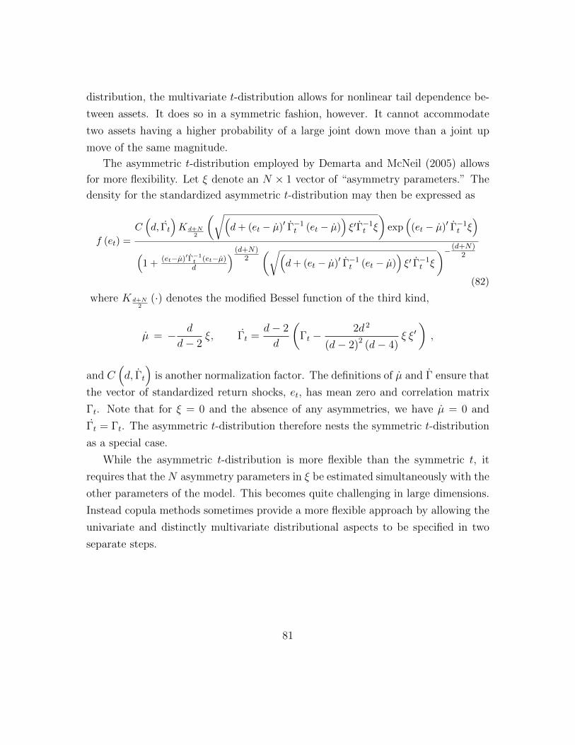
distribution, the multivariate t-distribution allows for nonlinear tail dependence be-

tween assets. It does so in a symmetric fashion, however. It cannot accommodate

two assets having a higher probability of a large joint down move than a joint up

move of the same magnitude.

The asymmetric t-distribution employed by Demarta and McNeil (2005) allows

for more flexibility. Let ξ denote an N × 1 vector of “asymmetry parameters.” The

density for the standardized asymmetric t-distribution may then be expressed as

f (et) =

C(d, Γt

)K d+N

2

(√(d+ (et − µ)′ Γ−1

t (et − µ))ξ′Γ−1

t ξ

)exp

((et − µ)′ Γ−1

t ξ)

(1 +

(et−µ)′Γ−1t (et−µ)d

) (d+N)2

(√(d+ (et − µ)′ Γ−1

t (et − µ))ξ′ Γ−1

t ξ

)− (d+N)2

(82)

where K d+N2

(·) denotes the modified Bessel function of the third kind,

µ = − d

d− 2ξ, Γt =

d− 2

d

(Γt −

2d 2

(d− 2)2 (d− 4)ξ ξ′),

and C(d, Γt

)is another normalization factor. The definitions of µ and Γ ensure that

the vector of standardized return shocks, et, has mean zero and correlation matrix

Γt. Note that for ξ = 0 and the absence of any asymmetries, we have µ = 0 and

Γt = Γt. The asymmetric t-distribution therefore nests the symmetric t-distribution

as a special case.

While the asymmetric t-distribution is more flexible than the symmetric t, it

requires that the N asymmetry parameters in ξ be estimated simultaneously with the

other parameters of the model. This becomes quite challenging in large dimensions.

Instead copula methods sometimes provide a more flexible approach by allowing the

univariate and distinctly multivariate distributional aspects to be specified in two

separate steps.

81

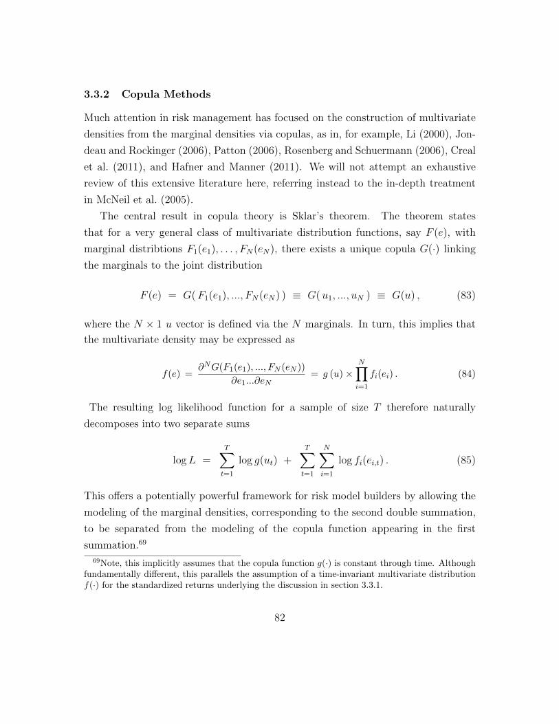
3.3.2 Copula Methods

Much attention in risk management has focused on the construction of multivariate

densities from the marginal densities via copulas, as in, for example, Li (2000), Jon-

deau and Rockinger (2006), Patton (2006), Rosenberg and Schuermann (2006), Creal

et al. (2011), and Hafner and Manner (2011). We will not attempt an exhaustive

review of this extensive literature here, referring instead to the in-depth treatment

in McNeil et al. (2005).

The central result in copula theory is Sklar’s theorem. The theorem states

that for a very general class of multivariate distribution functions, say F (e), with

marginal distribtions F1(e1), . . . , FN(eN), there exists a unique copula G(·) linking

the marginals to the joint distribution

F (e) = G(F1(e1), ..., FN(eN) ) ≡ G(u1, ..., uN ) ≡ G(u) , (83)

where the N × 1 u vector is defined via the N marginals. In turn, this implies that

the multivariate density may be expressed as

f(e) =∂NG(F1(e1), ..., FN (eN ))

∂e1...∂eN= g (u)×

N∏i=1

fi(ei) . (84)

The resulting log likelihood function for a sample of size T therefore naturally

decomposes into two separate sums

logL =T∑t=1

log g(ut) +T∑t=1

N∑i=1

log fi(ei,t) . (85)

This offers a potentially powerful framework for risk model builders by allowing the

modeling of the marginal densities, corresponding to the second double summation,

to be separated from the modeling of the copula function appearing in the first

summation.69

69Note, this implicitly assumes that the copula function g(·) is constant through time. Althoughfundamentally different, this parallels the assumption of a time-invariant multivariate distributionf(·) for the standardized returns underlying the discussion in section 3.3.1.

82

Of course, in order to actually implement this approach, we need to specify the

copula function g(·). The most commonly employed copula is constructed from the

multivariate normal distribution. It may be succinctly expressed as

g(ut; Γ∗t ) = |Γ∗t |− 1

2 exp

−1

2Φ−1(ut)

′(Γ∗−1t − I)Φ−1(ut)

, (86)

where Φ−1(ut) refers to the N × 1 vector of standard inverse univariate normals, and

the correlation matrix Γ∗t pertains to the N × 1 vector e∗t with typical element,

e∗i,t = Φ−1(ui,t ) = Φ−1(Fi (ei,t)). (87)

The normal copula has the advantage that it is relatively easy to work with. However,

even though it is more flexible than the standard multivariate normal distribution, for

many financial risk applications it does not allow for sufficient dependence between

tail events.

To remedy this an alternative copula model can be built from the multivari-

ate t-distribution. The resulting t-copula allows for tail dependence between the

marginal probabilities ui,t but only in a symmetric fashion. Going one step fur-

ther, an asymmetric t-copula may also be developed from the asymmetric multivari-

ate t-distribution discussed above. From a practical modeling perspective, t-copula

models have the potential to break the curse of dimensionality, which is otherwise

unavoidable in multivariate t-distributions when N is large. In particular, while

the asymmetric t distribution in (82) requires the simultaneous estimation of ξ and

d, amounting to a total of N + 1 parameters, when using the asymmetric t-copula

instead, it is possible to separately estimate each of the N marginal distributions

allowing for asset specific distributional features.70 The marginal distributions may

then be “tied” together using an asymmetric t-copula with only two parameters: a

scalar copula dG and a scalar copula asymmetry parameter ξG. This approach has

successfully been implemented by Christoffersen et al. (2011a).

70Of course, the need to estimate the N×N correlation matrix Γt further confound the estimationproblem.

83

Many other classes of copula functions exist as well. Most of these, however,

including the popular Gumbel and Clayton classes, are not yet operational in high

dimensions. An intriguing approach to overcoming this general dimensionality prob-

lem has recently been suggested by Oh and Patton (2011), who recommend relying

on a latent factor structure for the copula. Fully efficient estimation of this new

class of models is complicated by the lack of closed-form expression for the likelihood

function but it is relatively easy to do via simulation-based procedures that match

appropriate rank statistics. Oh and Patton (2011) find that this new approach works

well in an application involving one hundred individual stocks.71 It is too early to

tell how widely applicable this copula-factor structure is.

3.3.3 Combining GARCH and RCov

Another approach for obtaining full-fledged multivariate conditional return distri-

butions is to combine the realized covariance measures and GARCH style dynamic

specifications with specific distributional assumptions, along the lines of the pro-

cedures discussed in section 3.2.3 where the innovation distributions were specified

mostly to ensure tractable (quasi-likelihood) estimation of the underlying dynamic

model parameters.

For example, if the distributions adopted for each of the univariate return innova-

tion series in the GARCH specifications for the individual components of Dt in the

DCC-style decomposition in equation (45) are taken as exact representations of the

data generating process, this in principle defines a conditional one-step-ahead return

distribution given the estimated (and assumed to be constant) realized correlation

matrix. However, this is only tractable if simple, and restrictive, distributional as-

sumptions are imposed. Typically, this implies resorting to a multivariate normal

or student t-distribution for the return innovation vector. This severely limits the

complexity and realism in modeling the individual return innovations and volatili-

ties. Short-term multi-horizon forecasts may be similarly obtained, if one stipulates

71Their actual estimation results also suggest significant tail dependencies for most of the indi-vidual stocks in their sample, with the degree of tail dependence being stronger in crashes thanbooms.

84

that the correlation matrix remains constant. For longer horizons, however, the dy-

namics of the realized correlation matrix would need to be modeled separately. In

that situation the system quickly becomes analytically untractable, and simulation

techniques are required for obtaining the multi-horizon density forecasts.

Another possible route involves the HEAVY model introduced in equations (74)-

(77). Assuming both multivariate innovation distributions are truly Wishart, as

discussed in section 3.2.3, the model naturally delivers a complete characterization

of the one-step-ahead joint return distribution. The multi-horizon density forecasts

must again rely on Monte Carlo procedures.

As an alternative to these GARCH representations, there has recently been an

upsurge in work on related multivariate stochastic volatility models. These specifi-

cations generalize GARCH models in the sense that the dynamics of the volatility

process is governed by independent random shocks rather than a deterministic func-

tion of the return innovations. The models tend to be heavily parametric but they

may, under appropriate simplifying assumptions, be combined with realized covari-

ance matrix measures.72 These models typically exploit Gaussian assumptions for

the return and volatility (square-root covariance matrix) innovations as they produce

“squares” that are Wishart distributed and thus known in closed form.73

The additive component Wishart-RCOV-A(K) model in Jin and Maheu (2010)

provides an interesting example of combining such stochastic volatility representa-

tions with realized measures, by exploiting features akin to a multivariate HAR-RV

model for the individual components of the realized covariance matrix. Although the

empirical results appear promising, the parametric assumptions remain somewhat re-

strictive and estimation must be performed via Bayesian techniques using Markov

Chain Monte Carlo (MCMC) procedures that are tractable only for moderately sized

72Among the initial contributions in this area are Philipov and Glickman (2006), who specify astandard Wishart transition density for the inverse covariance matrix of daily returns, as well asGourieroux et al. (2009) who introduce the Wishart autoregressive model for daily data. Extensionsof these models that involve realized covariance measures have been developed by, e.g., Bonato et al.(2009), Golosnoy et al. (2010), and Asai and So (2010).

73The Wishart distribution provides the matrix generalization of a “squared” normal distribution,i.e., just as the sum of squared i.i.d. normal variates are χ2 distributed, the sampling distributionof the sample covariance matrix for draws from the multivariate normal distribution is Wishart.

85

systems.

To summarize, the work on incorporating time-varying realized covariance mea-

sures within the multivariate GARCH and related stochastic volatility model setting

is in its infancy. Given the need for tractability, the existing procedures invoke overly

simplistic distributional assumptions, rendering the multi-horizon density forecasts

unable to fully account for critical features such as pronounced return-volatility asym-

metries, the possibility of jumps, long memory style volatility dynamics, and extreme

correlations in down markets. For the time being, such features are more readily por-

trayed through the design of appropriate simulation methods.

3.3.4 Multivariate Simulation Methods

The multivariate normal distribution implies normally distributed portfolio returns

so that the V aR, ES and most other risk measures are easily computed analytically.

When using non-normal distributions, or any kind of copula, portfolio V aR and ES

must instead be computed via Monte Carlo simulation, rendering purely simulation-

based methods relatively more attractive.

In the general multivariate case, we can in principle use the Filtered Historical

Simulation (FHS) approach discussed in section 2.3.4, but a multivariate standard-

ization is needed. Using for example the Cholesky or the spectral decomposition we

first create vectors of standardized returns as in equation (78); i.e.,

Zt = Ω−1/2t Rt , t = 1, 2, . . . , T ,

where Ω−1/2t denotes the relevant decomposition of the estimated covariance matrix.74

Now, resampling with replacement vector-wise from the standardized returns will en-

sure that the marginal distributions, as well as particular features of the multivariate

distribution, as for example, the contemporaneous cross-sectional dependencies sug-

gested by Longin and Solnik (2001), will be preserved in the simulated data.

The dimensionality of the system may render the general multivariate standard-

74Patton and Sheppard (2009) recommend the spectral decomposition because unlike theCholesky, it is invariant to a reordering of the variables.

86

ization above practically infeasible. However, the same FHS approach can be applied

with the base asset setup discussed in section 3.1.2, resampling from the factor in-

novations,

ZF,t = Ω−1/2F,t RF,t , t = 1, 2, . . . ... , T ,

where we again rely on the spectral or Cholesky decomposition to build up the

distribution of the factor returns. Given the specification in section 3.1.2, the corre-

sponding idiosyncratic asset innovations may then be constructed from,

νt = Rt − B RF,t , t = 1, 2, . . . ... , T .

Thus, by resampling sequentially from Zt and νt, we can easily build up the required

distribution of the individual asset returns. This, of course, assumes that the base

asset model provides a good description of the joint dependencies.

Alternatively, if one is willing to assume constant conditional correlations, as

in equation (45) with Γt = Γ, then the standardization can simply be done on an

individual asset-by-asset basis using the univariate GARCH or RV-based predictive

volatilities. Resampling vector-wise from the standardized returns will naturally

preserve the cross-sectional dependencies in the historical data.

3.3.5 Multivariate Extreme Value Theory

The simulation procedures discussed above work well for numerically describing cor-

relations and related “central” features of the joint return distributions. Multivariate

Extreme Value Theory (EVT) offers a tool for exploring cross-asset dependencies in

the “tails” of distributions, which are not well-captured by standard parametric dis-

tributions or correlation measures.

For example, Longin and Solnik (2001) define and compute extreme correlations

between monthly U.S. index returns and a number of foreign country indexes. In

the case of the bivariate normal distribution, correlations between extremes taper off

to zero as the thresholds defining the extremes get larger in absolute value. Actual

financial returns, however, behave quite differently. In particular, the correlation

87

between the large (in an absolute sense) negative returns reported in Longin and

Solnik (2001) tend to be much larger than the normal distribution would suggest

(while interestingly, the correlations of large positive returns appear to approach

zero in accordance with the normal distribution).75 Such strong correlation between

negative extremes is clearly a key risk management concern.76

To illustrate the important deviations from multivariate normality commonly

found in financial markets, consider the threshold plots in Figure 12. The solid

lines in Figure 12 show the empirical equity index threshold correlations averaged

across the 120 possible pairs of correlations based on the same 16 developed market

returns used in the estimation of the DECO model in Figure 11. For comparison, the

dashed lines indicate the threshold correlations implied by a multivariate standard

normal distribution with constant correlation, while the lines with square markers are

the threshold correlations computed via simulations from the previously estimated

DECO model.

As the figure clearly shows, the down-market threshold correlations are much

stronger than the up-market correlations. The multivariate normal distribution with

constant correlation captures quite closely the up-market correlations but it cannot

simultaneously account for the much larger, and increasing with the threshold, down-

market correlations. The dynamic normal distribution driven by the basic Gaussian

DECO model generates larger threshold correlations overall, but the model does

not explain the strong multivariate asymmetry that actually exists in the returns.

The specification of dynamic multivariate models and distributions to satisfactorily

account for these important non-linear asymmetric extreme dependencies is challeng-

ing. It remains the focus of much ongoing work, much of which rely on the use of

copulas and/or EVT type approximations.

A full treatment of this literature, and the extensive literature on multivariate

75See also Ang and Bekaert (2002), Ang and Chen (2002) and Ang et al. (2006), among manyothers, for additional empirical evidence on similar nonlinear dependencies in equity returns.

76It is generally unclear where these increased dependencies in the “tails” are coming from. Poonet al. (2004), for instance, report that “devolatilizing” the daily returns for a set of internationalstock markets significantly reduces the joint tail dependence, while Bae et al. (2003) find that time-varying volatility and GARCH effects can not fully explain the counts of coincident “extreme” dailyprice moves observed across international equity markets.

88

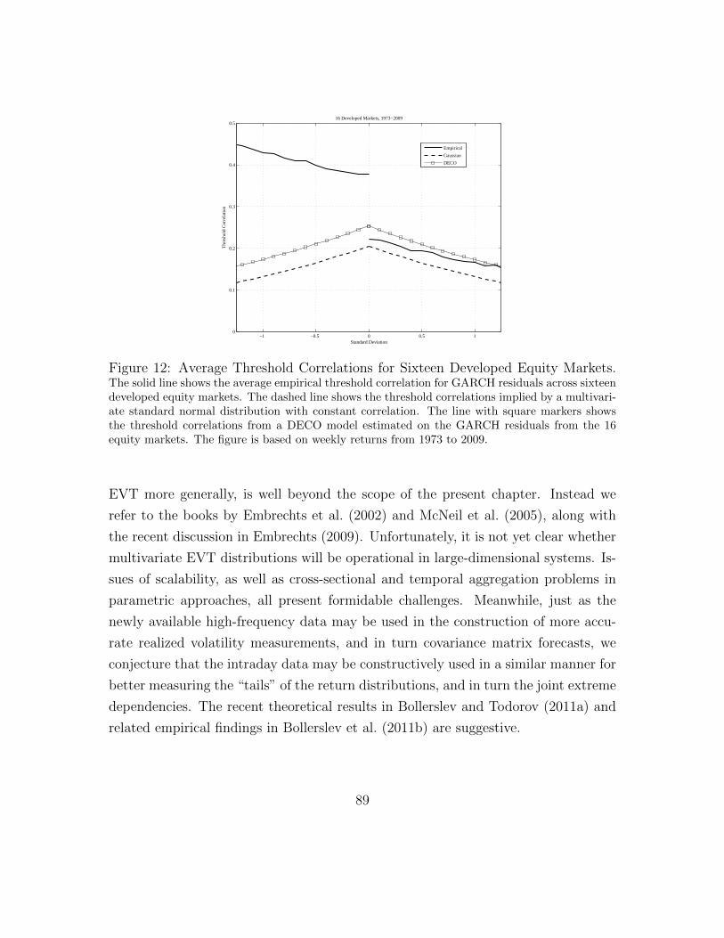
−1 −0.5 0 0.5 10

0.1

0.2

0.3

0.4

0.516 Developed Markets, 1973−2009

Thr

esho

ld C

orre

latio

n

Standard Deviation

Empirical

Gaussian

DECO

Figure 12: Average Threshold Correlations for Sixteen Developed Equity Markets.The solid line shows the average empirical threshold correlation for GARCH residuals across sixteendeveloped equity markets. The dashed line shows the threshold correlations implied by a multivari-ate standard normal distribution with constant correlation. The line with square markers showsthe threshold correlations from a DECO model estimated on the GARCH residuals from the 16equity markets. The figure is based on weekly returns from 1973 to 2009.

EVT more generally, is well beyond the scope of the present chapter. Instead we

refer to the books by Embrechts et al. (2002) and McNeil et al. (2005), along with

the recent discussion in Embrechts (2009). Unfortunately, it is not yet clear whether

multivariate EVT distributions will be operational in large-dimensional systems. Is-

sues of scalability, as well as cross-sectional and temporal aggregation problems in

parametric approaches, all present formidable challenges. Meanwhile, just as the

newly available high-frequency data may be used in the construction of more accu-

rate realized volatility measurements, and in turn covariance matrix forecasts, we

conjecture that the intraday data may be constructively used in a similar manner for

better measuring the “tails” of the return distributions, and in turn the joint extreme

dependencies. The recent theoretical results in Bollerslev and Todorov (2011a) and

related empirical findings in Bollerslev et al. (2011b) are suggestive.

89

3.4 Systemic Risk Definition and Measurement

The univariate portfolio-level and multivariate asset-level risk models discussed in

sections 2 and 3, respectively, may be used in the construction of real-time portfolio

risk measures, such as V aR and ES, conditional on the history of returns. It is

sometimes informative to also consider risk measures that condition not only on

historical returns, but also on assumed scenarios for particular risk factors. We

might, for example, be interested in the market-wide effects of a shock to a particular

firm.

Scenario-based conditional risk measures are also intrinsically related to systemic

risk. Systemic risk measures can help firms to develop richer and more informative

risk reports internally. They can also be used by supervisory authorities to measure

and monitor the contributions from individual firms to aggregate market risk, as well

as total (or average) systemic risk across all firms.

3.4.1 Marginal Expected Shortfall and Expected Capital Shortfall

Marginal expected shortfall (MES) for firm j is

MESj|mktT+1|T = ET [rj,T+1|C (rmkt,T+1)] , (88)

where rmkt,T+1 denotes the overall market return, and C (rmkt,T+1) denotes a systemic

event, such as the market return falling below some threshold C. MESj|mkt tracks

the sensitivity of firm j’s return to a market-wide extreme event, thereby providing

a simple market-based measure of firm j’s fragility.

Ultimately, however, we are interested in assessing the likelihood of firm distress,

and the fact that a firm’s expected return is sensitive to market-wide extreme events

– that is, the fact that its MES is large – does not necessarily mean that market-

wide extreme events are likely to place it in financial distress. Instead, the distress

likelihood should depend not only on MES, but also on how much capital the firm

has on hand to buffer the effects of adverse market moves.

These distress considerations raise the idea of expected capital shortfall (ECS),

90

which is closely related to, but distinct from, MES. ECS is the expected additional

capital needed by firm j in case of a systemic market event. Clearly ECS should be

related to MES, and Acharya et al. (2010) indeed show that in a simple model the

two are linearly related,

ECSj|mktT+1|T = a0j + a1jMES

j|mktT+1|T , (89)

where a0j depends on firm j’s “prudential ratio” of asset value to equity as well as

its debt composition, and a1j depends on firm j’s prudential ratio and initial capi-

tal. Based on this, Brownlees and Engle (2011) propose and empirically implement

ECSj|mktT+1|T as a measure of firm j’s systemic risk contribution to the market at time

T , with overall systemic risk then given by∑N

j=1ECSj|mktT+1|T .

Implementation of MES (and hence ECS) requires specification of the systemic

market event C (rmkt,T+1), or more simply a market return threshold C. Values

of C = 2% and C = 40% have, for example, been suggested for one-day and six-

month returns, respectively. In addition, and of crucial importance, implementation

of MES also requires a multivariate volatility model. That is, the conditioning on

C (rj,T+1) in all of the measures above, from MESj|mktT+1|T through to

∑Nj=1 ECS

j|mktT+1|T ,

requires at least a bivariate volatility model for firm and market returns, and more

generally a high-dimensional volatility model for all firms’ returns. The models

introduced in sections 3.1-3.3 satisfy that need.77

3.4.2 CoVaR and ∆CoVaR

We defined, in equation (1), firm j’s one-period ahead V aR at level p as the value

of V aRp,jT+1|T that solves,

p = PrT

(rj,T+1 < −V aRp,j

T+1|T

).

77Brownlees and Engle (2011), for example, use the daily GARCH-DCC modeling approachdescribed in section 3.1.1. Interestingly, they find that aggregate MES increased sharply startingin mid-2007, and that even by mid-2010 it was still much higher than in the pre-crisis period.

91

Similarly, following Adrian and Brunnermeier (2011), one may define firm j’s one-

period ahead “CoV aR” at level p conditional on a particular outcome for firm i, say

C (ri,T+1), as the value of CoV aRj|iT+1|T that solves,

p = PrT

(rj,T+1 < −CoV aRj|i

T+1|T | C (ri,T+1)). (90)

Because C (ri,T+1) is not in the time-T information set, CoV aR will be different from

the regular time-T conditional V aR. The leading choice of conditioning outcome,

C (ri,T+1), is that firm i exceeds its V aR, or more precisely that ri,T+1 < −V aRp,iT+1|T .

As such, CoV aR is well-suited to measure tail-event linkages between financial in-

stitutions.

A closely-related measure, ∆CoV aRj|iT+1|T (read “Delta CoV aR”), is of particular

interest. It measures the difference between firm-j V aR when firm-i is “heavily”

stressed and firm-j V aR when firm i experiences “normal” times. More precisely,

∆CoV aRj|iT+1|T = CoV aR

j|V aR(i)T+1|T − CoV aRj|Med(i)

T+1|T , (91)

where CoV aRj|V aR(i)T+1|T denotes firm-j V aR when firm i’s return breaches its V aR and

CoV aRj|Med(i)T+1|T denotes firm-j V aR when firm i’s return equals its median.

A direct extension lets us progress to the more interesting case of firm i’s overall

systemic risk, as opposed to just firm i’s impact on firm j. We simply set j = sys,

where sys denotes the financial system as a whole, as measured by the return on

a portfolio of all financial institutions. ∆CoV aRsys|iT+1|T then measures the difference

between financial system V aR conditional on firm i experiencing an extreme re-

turn, and financial system V aR conditional on firm i experiencing a normal return.

Hence ∆CoV aRsys|iT+1|T measures the contribution of firm i to the overall systemic risk,∑N

i=1 ∆CoV aRsys|iT+1|T .78

The conditioning on C (ri,T+1) in all of the CoV aRmeasures above, from CoV aRj|iT+1|T

through to∑N

i=1 ∆CoV aRsys|iT+1|T , requires at least a bivariate volatility model for the

78The concept of CoV aR also has interesting parallels to the conditioning of V aR in Garcia et al.(2007), who show that proper conditioning in V aR can eliminate the subadditivity problems raisedby Artzner et al. (1999).

92

returns on firms i and j, or i and sys, and more generally a high-dimensional volatil-

ity model for all firms’ returns. The models introduced in sections 3.1-3.3 are again

relevant.79

3.4.3 Network Perspectives

Interestingly, modern network theory provides a powerful unifying framework for

systemic risk measures, including measures like CoV aR introduced above.80 The

simplest network is composed of N nodes, where any given pair of nodes may or

may not be linked. We represent the network algebraically by an N ×N symmetric

adjacency matrix A of zeros and ones, A = [aij], where aij = 1 if nodes i and j

are linked, and aij = 0 otherwise. Because all network properties are embedded in

A, any sensible connectedness measure must be based on A. The most important

and popular, by far, are based on the idea of a node’s degree, given by the number

of its links to other nodes δi =∑

j aij, as well as aspects of the degree distribution

across nodes. The total degree Σiδi (or mean degree 1N

Σiδi) is the key network

connectedness measure.

The network structure sketched above is, however, rather too simple to describe

the network connections of relevance in financial risk management (e.g., among fi-

nancial institution equity returns). Generalization in two key directions is neces-

sary. First, links may be of varying strength, not just 0-1. Second, links may be

of different strength in different directions (e.g., firm i may impact firm j more

than firm j impacts firm i). Note, for example, that the systemic risk measures

introduced above are weighted and directional. For example, CoV aRj|iT+1|T tracks

effects from i to j, whereas CoV aRi|jT+1|T tracks effects from j to i, and in general

CoV aRj|iT+1|T 6= CoV aR

i|jT+1|T .

It is a simple matter, however, to characterize directed, weighted networks in a

parallel fashion. To allow for directionality, we allow the adjacency matrix A to be

79Multivariate quantile models, such as those recently developed by White et al. (2010), couldalso be used in this context.

80Here we provide a brief overview of key ideas. Extended discussion, references, and systemic riskmeasures based directly on network topology are contained in Diebold and Yilmaz (2009, 2011a,b).

93

non-symmetric, and to allow for different relationship strengths we allow A to contain

weights aij ∈ [0, 1] rather than simply 0-1 entries. Node degrees are now obtained

by summing weights rather than zeros and ones, and there are now “to-degrees” and

“from-degrees,” corresponding to row sums and column sums, which generally differ

since A is generally non-symmetric. The from-degree of node i is δfromi =∑

j aij,

and the to-degree of node j is δtoj =∑

i aij. The total degree is δ = Σiδfromi = Σjδ

toj .

Crucially, the from-, to- and total degrees measure systemic impacts. The from-

and to-degrees measure systemic risk with respect to particular firms; from degrees

measure systemic impacts from the system to a given firm, and to-degrees measure

systemic impacts from a given firm to the system. The total degree aggregates firm-

specific systemic risk across firms, providing a measure of total system-wide systemic

risk. The key insight is that many approaches to systemic risk measurement fit

naturally into the just-described network framework. Consider, for example, the

earlier-discussed ∆CoV aR measure. One can arrange ∆CoV aRj|iT+1|T , i, j = 1, ..., N

as elements (aji) of an adjacency matrix that defines a weighted directed network of

firms. Then, for example, the systemic risk of firm i, ∆CoV aRsys|iT+1|T , is the network

to-degree of firm i, δtoi = Σj∆CoV aRj|iT+1|T . And finally, the total systemic risk,∑

i ∆CoV aRsys|iT+1|T , is the network total degree δ.

4 Conditioning on Macroeconomic Fundamentals

The risk models that we have discussed thus far are inherently “reduced form,”

in nature. They explain risk in an autoregressive fashion, as exemplified by the

canonical GARCH family. Fortunately, even if the models fail to provide a deep

structural understanding of volatility movements, they are nevertheless powerful and

useful in a variety of contexts. We have obviously emphasized risk measurement and

management, but other successful areas of application include portfolio allocation,

spot and derivative asset pricing, active trading, and dynamic hedging.

Ultimately, however, we aspire to a deeper structural understanding. That is, we

aspire to understand the connections between returns (especially, for our purposes,

return volatilities) and macroeconomic fundamentals, say r ↔ f . Asset prices are

94

µr - σr

-

-

µf

?

6

- σf

?

6

Figure 13: Return and Fundamental Mean and Volatility Linkages. Each link representsa distinct line of inquiry.

risk-adjusted discounted claims on fundamental streams, so prices and their proper-

ties should ultimately depend on expected fundamentals and associated fundamental

risks. Here we sketch emerging empirical aspects of those connections, through the

lens of return and fundamental first and second moments, denoted µr, σr, µf , and σf ,

respectively.81 Figure 13 provides a simple schematic diagram for all of the possible

connections among σr, µr, σf , and µf . Each of the six connections represents a po-

tentially important link, and a correspondingly important line of research inquiry.82

Historically, however, it is well-known that σr, µr, σf , and µf have often ap-

peared only weakly connected, or even disconnected. This observation is memorably

enshrined in equity markets in the “excess volatility” puzzle of Shiller (1981), in

foreign exchange markets in the “exchange rate disconnect” puzzle of Obstfeld and

Rogoff (2000), in bond markets in Alan Greenspan’s long-maturity yield “conun-

drum,” and so on.83

81In parallel to the models for returns emphasized so far in this chapter, we will content ourselveswith means and variances, but one could, of course, also consider higher-order moments.

82Note that the links in Figure 13 are “undirected,” or “non-causal,” and as such more aboutcorrelation than causation. One could go even farther and consider directed, or causal, links, butthat would require replacing each bi-directional arrow in Figure 13 with a pair of uni-directionalarrows, thus doubling the number of links to be addressed.

83On the conundrum: “ ... the broadly unanticipated behavior of world bond markets remainsa conundrum. Bond price movements may be a short-term aberration, but it will be some timebefore we are able to better judge the forces underlying recent experience” [Alan Greenspan, U.S.congressional testimony, February 16, 2005]; see also Backus and Wright (2007).

95

In contrast, we shall present and interpret a variety of accumulating evidence

showing how returns – return volatilities in particular – are connected to fundamen-

tals. Of course many of the links in Figure 13 remain incompletely understood, but

they are receiving increased attention, and volatility features prominently through-

out this emerging research. Given the theme of the chapter, we will focus largely on

three links directly involving σr and/or σf , namely µf ↔ σr, µf ↔ σf , and σf ↔ σr.

We now address them in turn.

4.1 The Macroeconomy and Return Volatility

To begin, consider the link between macroeconomic fundamentals and return volatil-

ity, µf ↔ σr. Officer (1973) was among the first to document and emphasize the

very high stock market volatility during the very severe recession of the 1930s. The

U.S. stock market crash of 1987 spurred additional research into the fundamental

determinants of volatility. In a well-known and exhaustive study in the wake of the

1987 crash, for example, Schwert (1989) went farther, showing that, surprisingly, the

oft-suspected fundamentals (leverage, corporate profitability, etc.) have negligible

impact on market volatility, while recessions do. In particular, return volatility is

significantly higher in recessions, so that high volatility during bad times is not just

a one-off Great Depression phenomenon, but rather a regularly-recurring business

cycle phenomenon.

These findings regarding the link between financial market volatility and the busi-

ness cycle have since been echoed repeatedly. Hamilton and Lin (1996), for example,

provide strong and sophisticated confirmation using regime-switching models of real

growth and equity returns, allowing for both high and low real growth states and

high and low equity return volatility states. Their estimated regime transition prob-

abilities indicate high positive steady-state coherence between low (high) real growth

and high (low) equity return volatility.

More recent work, in particular Bloom et al. (2009) as summarized in Table 1,

also confirms and significantly amplifies Schwert’s earlier result, showing, among

other things, that it holds not only for stock returns at the aggregate level, but

96

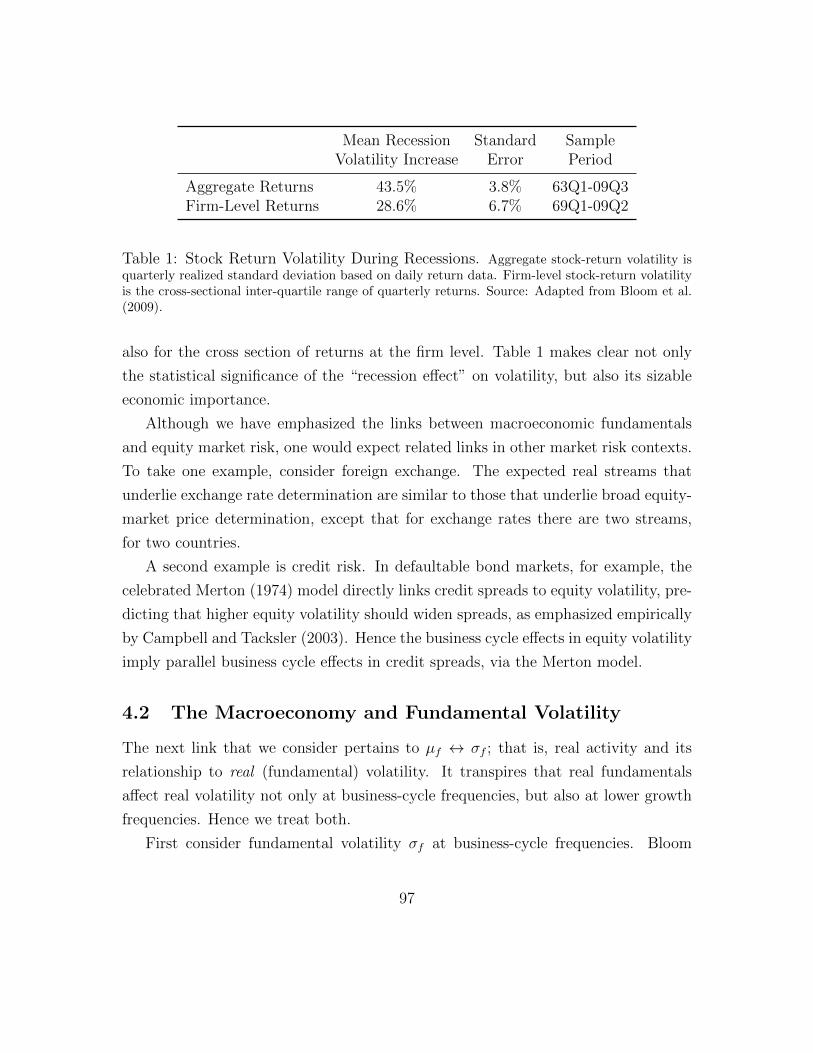
Mean Recession Standard SampleVolatility Increase Error Period

Aggregate Returns 43.5% 3.8% 63Q1-09Q3Firm-Level Returns 28.6% 6.7% 69Q1-09Q2

Table 1: Stock Return Volatility During Recessions. Aggregate stock-return volatility isquarterly realized standard deviation based on daily return data. Firm-level stock-return volatilityis the cross-sectional inter-quartile range of quarterly returns. Source: Adapted from Bloom et al.(2009).

also for the cross section of returns at the firm level. Table 1 makes clear not only

the statistical significance of the “recession effect” on volatility, but also its sizable

economic importance.

Although we have emphasized the links between macroeconomic fundamentals

and equity market risk, one would expect related links in other market risk contexts.

To take one example, consider foreign exchange. The expected real streams that

underlie exchange rate determination are similar to those that underlie broad equity-

market price determination, except that for exchange rates there are two streams,

for two countries.

A second example is credit risk. In defaultable bond markets, for example, the

celebrated Merton (1974) model directly links credit spreads to equity volatility, pre-

dicting that higher equity volatility should widen spreads, as emphasized empirically

by Campbell and Tacksler (2003). Hence the business cycle effects in equity volatility

imply parallel business cycle effects in credit spreads, via the Merton model.

4.2 The Macroeconomy and Fundamental Volatility

The next link that we consider pertains to µf ↔ σf ; that is, real activity and its

relationship to real (fundamental) volatility. It transpires that real fundamentals

affect real volatility not only at business-cycle frequencies, but also at lower growth

frequencies. Hence we treat both.

First consider fundamental volatility σf at business-cycle frequencies. Bloom

97

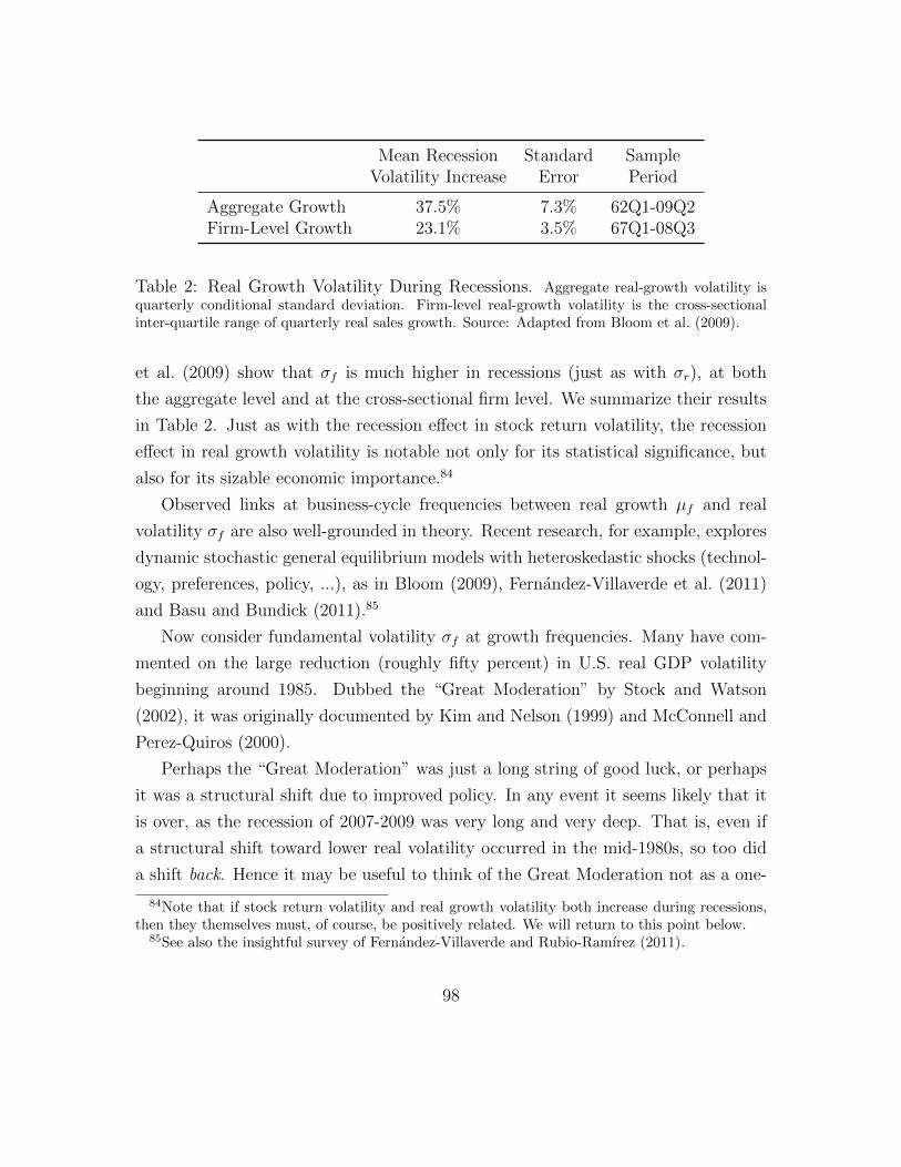
Mean Recession Standard SampleVolatility Increase Error Period

Aggregate Growth 37.5% 7.3% 62Q1-09Q2Firm-Level Growth 23.1% 3.5% 67Q1-08Q3

Table 2: Real Growth Volatility During Recessions. Aggregate real-growth volatility isquarterly conditional standard deviation. Firm-level real-growth volatility is the cross-sectionalinter-quartile range of quarterly real sales growth. Source: Adapted from Bloom et al. (2009).

et al. (2009) show that σf is much higher in recessions (just as with σr), at both

the aggregate level and at the cross-sectional firm level. We summarize their results

in Table 2. Just as with the recession effect in stock return volatility, the recession

effect in real growth volatility is notable not only for its statistical significance, but

also for its sizable economic importance.84

Observed links at business-cycle frequencies between real growth µf and real

volatility σf are also well-grounded in theory. Recent research, for example, explores

dynamic stochastic general equilibrium models with heteroskedastic shocks (technol-

ogy, preferences, policy, ...), as in Bloom (2009), Fernandez-Villaverde et al. (2011)

and Basu and Bundick (2011).85

Now consider fundamental volatility σf at growth frequencies. Many have com-

mented on the large reduction (roughly fifty percent) in U.S. real GDP volatility

beginning around 1985. Dubbed the “Great Moderation” by Stock and Watson

(2002), it was originally documented by Kim and Nelson (1999) and McConnell and

Perez-Quiros (2000).

Perhaps the “Great Moderation” was just a long string of good luck, or perhaps

it was a structural shift due to improved policy. In any event it seems likely that it

is over, as the recession of 2007-2009 was very long and very deep. That is, even if

a structural shift toward lower real volatility occurred in the mid-1980s, so too did

a shift back. Hence it may be useful to think of the Great Moderation not as a one-

84Note that if stock return volatility and real growth volatility both increase during recessions,then they themselves must, of course, be positively related. We will return to this point below.

85See also the insightful survey of Fernandez-Villaverde and Rubio-Ramırez (2011).

98

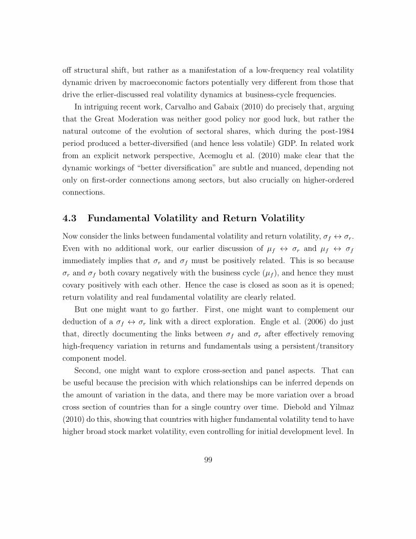
off structural shift, but rather as a manifestation of a low-frequency real volatility

dynamic driven by macroeconomic factors potentially very different from those that

drive the erlier-discussed real volatility dynamics at business-cycle frequencies.

In intriguing recent work, Carvalho and Gabaix (2010) do precisely that, arguing

that the Great Moderation was neither good policy nor good luck, but rather the

natural outcome of the evolution of sectoral shares, which during the post-1984

period produced a better-diversified (and hence less volatile) GDP. In related work

from an explicit network perspective, Acemoglu et al. (2010) make clear that the

dynamic workings of “better diversification” are subtle and nuanced, depending not

only on first-order connections among sectors, but also crucially on higher-ordered

connections.

4.3 Fundamental Volatility and Return Volatility

Now consider the links between fundamental volatility and return volatility, σf ↔ σr.

Even with no additional work, our earlier discussion of µf ↔ σr and µf ↔ σf

immediately implies that σr and σf must be positively related. This is so because

σr and σf both covary negatively with the business cycle (µf ), and hence they must

covary positively with each other. Hence the case is closed as soon as it is opened;

return volatility and real fundamental volatility are clearly related.

But one might want to go farther. First, one might want to complement our

deduction of a σf ↔ σr link with a direct exploration. Engle et al. (2006) do just

that, directly documenting the links between σf and σr after effectively removing

high-frequency variation in returns and fundamentals using a persistent/transitory

component model.

Second, one might want to explore cross-section and panel aspects. That can

be useful because the precision with which relationships can be inferred depends on

the amount of variation in the data, and there may be more variation over a broad

cross section of countries than for a single country over time. Diebold and Yilmaz

(2010) do this, showing that countries with higher fundamental volatility tend to have

higher broad stock market volatility, even controlling for initial development level. In

99

the most thorough study to date, Engle and Rangel (2008) explore time-series, cross-

sections and panels, clearly finding that the “long-term volatilities of macroeconomic

fundamentals ... are primary causes of low-frequency market volatility.”

In closing this section we note that we have largely interpreted “market risk and

macro fundamentals” as “market volatility and macro fundamentals.” As we have

emphasized earlier in our discussion of portfolio-level risk measurement, however,

one may naturally approach market volatility from a top-down (portfolio-level) or

bottom-up (asset-level) perspective. In a bottom-up approach, not only conditional

variances but also conditional correlations among individual returns are of central

importance as they obviously impact portfolio (i.e., market) volatility. Hence the

fundamental determinants of conditional correlations have also recently begun to

receive attention, as in Engle and Rangel (2011).

4.4 Other Links

The links between volatility and fundamentals that we have discussed thus far do not

involve µr. There are two main reasons. First, the horizons emphasized throughout

most of the chapter tend to be fairly short – typically less than a month – and at such

short horizons µr is small and arguably almost constant.86 Second, at longer horizons

for which µr is larger and likely time-varying in interesting ways, we can interpret

µr as an excess return (“the equity premium”), which, of course, is the subject of an

enormous and distinguished literature that is treated extensively elsewhere in this

volume. Hence we provide here only brief glimpses of aspects of the links µr ↔ σr,

µr ↔ µf and µr ↔ σf as they relate most directly to our present concerns.

First, consider the equity premium and return-volatility relationship, µr ↔ σr.

Stimulated by the pioneering work of Markowitz (1959), an enormous amount of asset

pricing research has focused on quantifying various aspects of this financial market

“risk-return tradeoff.” Financial econometric research has followed suit, as exempli-

fied by the GARCH-M model of Engle et al. (1987), defined by equations (7) and (8)

above with µt = x′tβ + δσt. In this model the conditional standard deviation enters

86Indeed that is why we typically fix µr at zero in previous sections.

100

directly as an explanatory variable for the conditional mean – together with other

possible explanatory variables xt – thus providing an econometric approximation to

a time-varying risk premium.87

Although intuitively appealing, a number of subtleties have emerged in both the-

ory and empirics. Modern general equilibrium theory reveals that, in principle, pos-

itive contemporaneous risk-return correlation is not guaranteed, as subtle dynamic

interactions may be operative; see, e.g., Abel (1988), Backus and Gregory (1993),

Whitelaw (2000), and Bollerslev et al. (2011a) among others. In parallel, a wealth

of recent empirical work reveals that, in practice, the contemporaneous risk-return

correlation is often found to be negative; see, e.g., Bollerslev et al. (2006), Lettau and

Ludvigson (2010) and Brandt and Wang (2010). Hence, rather ironically, we now

realize that we know less than we thought about the most-researched connection,

µr ↔ σr.

Second, consider the relationship between the equity premium and the business

cycle, µr ↔ µf . Fama and French (1989) and Fama (1990) emphasize expected busi-

ness conditions as a likely key driver of expected excess returns, with expected excess

returns negative near business cycle peaks and positive near troughs. However, they,

and the huge ensuing literature, use mostly proxies for expected business conditions,

typically the dividend yield, the term premium, and the default premium; see, e.g.,

Campbell and Thompson (2008) and the literature cited therein.88

Lettau and Ludvigson (2001) began a movement toward explicit incorporation of

expected business condition variables with their celebrated generalized consumption-

wealth ratio cay, or more precisely, the cointegrating residual between log consump-

tion and log wealth. Campbell and Diebold (2009), and subsequently Goetzman

et al. (2009), extended the movement with direct inclusion of expected real growth,

or more precisely, Livingston survey expectations of real growth.89 The results sug-

gest that expected growth is indeed a central determinant of expected excess returns,

with the Livingston expectations generally the most stable and significant predictor

87The conditional standard deviation is sometimes replaced by the conditional variance, µt =x′tβ + δσ2

t , or other monotone transformations of σt, in the estimation of the GARCH-M model.88Note that, ironically, the standard proxies are financial rather than real.89For details on the Livingston survey, see Croushore (1997).

101

across numerous competing specifications, including ones involving the “standard”

financial predictor variables.

Having discussed a number of links involving fundamental volatility, we are now

in a position to consider the final link, which also involves fundamental volatility,

namely µr ↔ σf . Modern asset-pricing theory emphasizes not only fundamental

expectations, but also fundamental volatilities in the determination of the equity

premium. An obvious example is the “long-run risk” model by Bansal and Yaron

(2004), and its extension explicitly incorporating time-varying economic uncertainty

in Bollerslev et al. (2009b). In this new class of models, which features Epstein

and Zin (1989) preferences, variation in both consumption’s conditional mean and

conditional variance contribute importantly to variation in the equity premium. Sup-

porting empirical evidence is provided in Bansal et al. (2005) and Bollerslev et al.

(2011a), among others.

4.5 Factors as Fundamentals

In our discussion of the the links between market risk and macro fundamentals we

have sometimes been casual in distinguishing returns from excess returns, realized

from expected returns, realized from expected volatility, and related, in our treatment

of timing. This is to some extent unavoidable, reflecting different conventions both

within and among different and evolving literatures, as well as our desire to convey

wide-ranging ideas in this broad survey. Nevertheless, a clearly-emergent theme

is that financial markets, as summarized by µr and σr, are very much linked to the

business cycle, as summarized by µf and σf . Indeed it is not an exaggeration to claim

that business cycle risk may be the key driver of expected excess equity returns and

return volatilities. Here we expand on that insight.

Although the business cycle may be a key risk factor, a long tradition, dating at

least to Burns and Mitchell (1946) and actively extending to the present, recognizes

that no single observed variable is “the business cycle” or “real activity.” Instead, we

observe literally dozens of indicators (employment, industrial production, GDP, per-

sonal income, etc.), all of which contain information about the business cycle, which

102

is not directly observable. Hence the key business cycle real activity fundamental

underlying risk may be appropriately and productively viewed as a common factor

to be extracted from many individual real activity indicators.

Expanding on this “factors as fundamentals” perspective, another likely-relevant

additional factor candidate is price/wage pressure, which may of course interact with

real activity, as emphasized in Aruoba and Diebold (2010). In any event, the point is

simply that, although we see hundreds of macroeconomic fundamentals, a drastically

smaller set of underlying macroeconomic factors is likely relevant for tracking market

risk. This is useful not only for best-practice firm-level risk management, but also

for regulators. In particular, the factors-as-fundamentals perspective has important

implications for the design of stress tests that simulate financial market responses to

fundamental shocks, suggesting that only a few key fundamentals (factors) need be

stressed.

Not surprisingly, then, we advocate that risk managers pay closer attention to

macroeconomic factors, as they are the ultimate drivers of market risk. We hasten to

add, however, that due to the frequent “disconnect” problems mentioned earlier, we

would never advocate conditioning risk assessments only on macroeconomic factors.

Rather, macroeconomic factors complement, rather than substitute, for the meth-

ods discussed in earlier sections, by broadening the conditioning information set to

include fundamentals in addition to past returns.

One might reasonably question the usefulness of conditioning on macroeconomic

data for daily risk assessment, because macroeconomic data are typically available

only quarterly (e.g., GDP and its components), or sometimes monthly (e.g., indus-

trial production and the CPI). Recent developments that exploit state space methods

and optimal filtering, however, facilitate high-frequency (e.g., daily) monitoring of la-

tent macroeconomic fundamental factors. In particular, based on the high-frequency

real activity monitoring approach of Aruoba et al. (2009), the Federal Reserve Bank

of Philadelphia produces the “ADS index” of real activity, updated and written to

the web in real time as new indicator data, released at different frequencies, are

released or revised.90

90The index and a variety of related materials are available at http://www.philadelphiafed.

103

We have emphasized macroeconomic fundamentals for equity market risk, but the

bond market is also closely linked to macroeconomic fundamentals. In particular,

government bond yield curves are driven by just a few factors (level, slope, curvature),

with the level factor closely linked to price/wage activity and the slope factor closely

linked to real activity.91 The same is true for yield curves of defaultable bonds, except

that there is the additional complication of default risk, but that too is linked to the

business cycle. Hence despite data on dozens of government bond yields, and dozens

of macroeconomic indicators, the interesting reality is their much lower-dimensional

“state vectors” – the level and slope factors beneath the yield curve, and the real

and price/wage activity factors beneath the macroeconomy. One can easily imagine

the usefulness for daily market and credit risk management (say) of systems linking

yield curve factors (level, slope, curvature, ...), equity factors (market, HML, SMB,

momentum, liquidity, ...), and macroeconomic factors (real, price/wage, ...). All of

those factors are now readily available at daily frequency.

5 Concluding Remarks

We have attempted to demonstrate the power and potential of dynamic financial

econometric methods for practical financial risk measurement and management. We

have surveyed the large literature on high-frequency volatility modeling, interpreting

and unifying the most important and intriguing results of practical relevance.92 Our

discussion has many implications for practical financial risk management; some point

toward desirable extensions of existing approaches, and some suggest new directions.

Key points include:

1. Standard “model-free” methods, such as historical simulation, rely on false

org/research-and-data/real-time-center/business-conditions-index.91For background and references, see Diebold and Rudebusch (2012).92We hasten to add that this chapter is a complement, not a substitute, for the more general and

technical survey of volatility and covariance forecasting of Andersen et al. (2006a). In addition,space constraints and other considerations have invariably limited our choice of included topics.For instance, we have largely neglected stochastic volatility and other parameter-driven approachesto volatility modeling, as well as option-implied volatility.

104

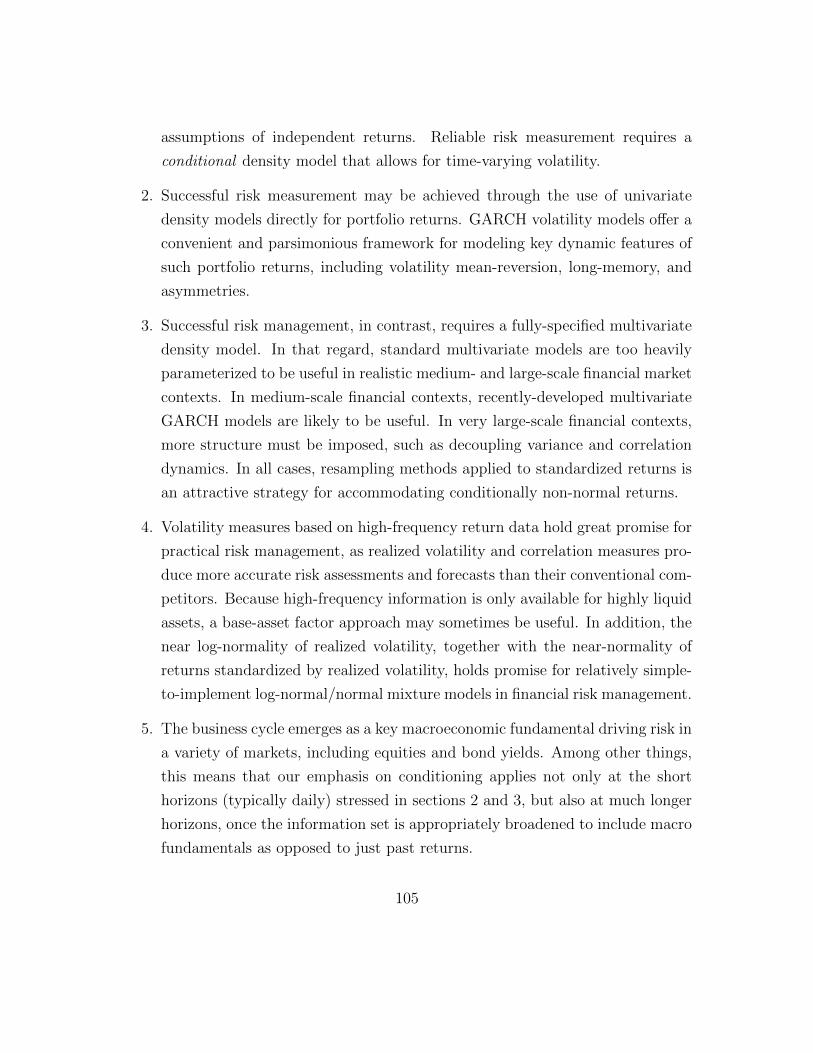
assumptions of independent returns. Reliable risk measurement requires a

conditional density model that allows for time-varying volatility.

2. Successful risk measurement may be achieved through the use of univariate

density models directly for portfolio returns. GARCH volatility models offer a

convenient and parsimonious framework for modeling key dynamic features of

such portfolio returns, including volatility mean-reversion, long-memory, and

asymmetries.

3. Successful risk management, in contrast, requires a fully-specified multivariate

density model. In that regard, standard multivariate models are too heavily

parameterized to be useful in realistic medium- and large-scale financial market

contexts. In medium-scale financial contexts, recently-developed multivariate

GARCH models are likely to be useful. In very large-scale financial contexts,

more structure must be imposed, such as decoupling variance and correlation

dynamics. In all cases, resampling methods applied to standardized returns is

an attractive strategy for accommodating conditionally non-normal returns.

4. Volatility measures based on high-frequency return data hold great promise for

practical risk management, as realized volatility and correlation measures pro-

duce more accurate risk assessments and forecasts than their conventional com-

petitors. Because high-frequency information is only available for highly liquid

assets, a base-asset factor approach may sometimes be useful. In addition, the

near log-normality of realized volatility, together with the near-normality of

returns standardized by realized volatility, holds promise for relatively simple-

to-implement log-normal/normal mixture models in financial risk management.

5. The business cycle emerges as a key macroeconomic fundamental driving risk in

a variety of markets, including equities and bond yields. Among other things,

this means that our emphasis on conditioning applies not only at the short

horizons (typically daily) stressed in sections 2 and 3, but also at much longer

horizons, once the information set is appropriately broadened to include macro

fundamentals as opposed to just past returns.

105

References

Abel, A. (1988), “Stock Prices Under Time-Varying Dividend Risk,” Journal of Monetary

Economics, 35, 375–393.

Acemoglu, D., A. Ozdaglar, and A. Tahbaz-Salehi (2010), “Cascades in Networks and

Aggregate Volatility,” Manuscript, MIT.

Acharya, V., L. Pedersen, T. Philippon, and M. Richardson (2010), “Measuring Systemic

Risk,” Manuscript, NYU.

Adrian, T. and M. Brunnermeier (2011), “CoVaR,” Manuscript, Federal Reserve Bank of

New York.

Aielli, G.P. (2006), “Consistent Estimation of Large Scale Dynamic Conditional Correla-

tions,” Manuscript, University of Florence.

Aıt-Sahalia, Y., P.A. Mykland, and L. Zhang (2011), “Ultra High Frequency Volatility

Estimation with Dependent Microstructure Noise,” Journal of Econometrics, 160,

190–203.

Albanese, C., K. Jackson, and P. Wiberg (2004), “A New Fourier Transform Algorithm for

Value-at-Risk,” Quantitative Finance, 4, 328–338.

Alexander, C. (2001), Market Models: A Guide to Financial Data Analysis, John Wiley

and Sons.

Alizadeh, S., M.W. Brandt, and F.X. Diebold (2002), “Range-Based Estimation of Stochas-

tic Volatility Models,” Journal of Finance, 57, 1047–1091.

Andersen, T. G. and T. Bollerslev (1997), “Heterogeneous Information Arrivals and Return

Volatility Dynamics: Uncovering the Long-Run in High-Frequency Returns,” Journal

of Finance, 52, 975–1005.

Andersen, T. G. and T. Bollerslev (1998a), “Answering the Skeptics: Yes, Standard Volatil-

ity Models do Provide Accurate Forecasts,” International Economic Review , 39, 885–

905.

106

Andersen, T. G. and T. Bollerslev (1998b), “DM-Dollar Volatility: Intraday Activity Pat-

terns, Macroeconomic Announcements, and Longer-Run Dependencies,” Journal of

Finance, 53, 219–265.

Andersen, T. G., T. Bollerslev, P.F. Christoffersen, and F.X. Diebold (2006a), “Volatility

and Correlation Forecasting,” In G. Elliot, C.W.J. Granger and A. Timmermann (eds.),

Handbook of Economic Forecasting, North-Holland, 777-878.

Andersen, T. G., T. Bollerslev, F. X. Diebold, and P. Labys (2003a), “Modeling and

Forecasting Realized Volatility,” Econometrica, 71, 579–625.

Andersen, T. G., T. Bollerslev, and F.X Diebold (2007a), “Roughing It Up: Including

Jump Components in the Measurement, Modeling and Forecasting of Return Volatil-

ity,” Review of Economics and Statistics, 89, 701–720.

Andersen, T. G., T. Bollerslev, and F.X. Diebold (2010a), “Parametric and Nonparamet-

ric Volatility Measurement,” In L.P. Hansen and Y. Aıt-Sahalia (eds.), Handbook of

Financial Econometrics, North-Holland, 67-138.

Andersen, T. G., T. Bollerslev, F.X. Diebold, and P. Labys (2000a), “Exchange Rate

Returns Standardized by Realized Volatility are (Nearly) Gaussian,” Multinational Fi-

nance Journal , 4, 159–179.

Andersen, T. G., T. Bollerslev, F.X. Diebold, and C. Vega (2003b), “Micro Effects of

Macro Announcements: Real-Time Price Discovery in Foreign Exchange,” American

Economic Review , 93, 38–62.

Andersen, T. G., T. Bollerslev, F.X. Diebold, and C. Vega (2007b), “Real-Time Price Dis-

covery in Global Stock, Bond and Foreign Exchange Markets,” Journal of International

Economics, 73, 251–277.

Andersen, T. G., T. Bollerslev, F.X. Diebold, and G. Wu (2006b), “Realized Beta: Persis-

tence and Predictability,” In T.B. Fomby and D. Terrell (eds.), Advances in Economet-

rics: Econometric Analysis of Economic and Financial Time Series, Elsevier, 1-40.

Andersen, T. G., T. Bollerslev, and D. Dobrev (2007c), “No-Arbitrage Semi-Martingale

Restrictions for Continuous-Time Volatility Models subject to Leverage Effects, Jumps

107

and i.i.d. Noise: Theory and Testable Distributional Assumptions,” Journal of Econo-

metrics, 138, 125–180.

Andersen, T. G., T. Bollerslev, P.H. Frederiksen, and M. Nielsen (2010b), “Continuous-

Time Models, Realized Volatilities, and Testable Distributional Implications for Daily

Stock Returns,” Journal of Applied Econometrcs, 25, 233–261.

Andersen, T. G., T. Bollerslev, and S. Lange (1999), “Forecasting Financial Market Volatil-

ity: Sample Frequency vis-a-vis Forecast Horizon,” Journal of Empirical Finance, 6,

457–477.

Andersen, T. G., T. Bollerslev, and N. Meddahi (2004), “Analytical Evaluation of Volatility

Forecasts,” International Economic Review , 45, 1079–1110.

Andersen, T. G., T. Bollerslev, and N. Meddahi (2011a), “Market Microstructure Noise

and Realized Volatility Forecasting,” Journal of Econometrics, 160, 220–234.

Andersen, T. G., D. Dobrev, and E. Schaumburg (2010c), “Jump-Robust Volatility Esti-

mation Using Nearest Neighbor Truncation,” Journal of Econometrics, forthcoming.

Andersen, T. G., D. Dobrev, and E. Schaumburg (2011b), “A Functional Filtering and

Neighborhood Truncation Approach to Integrated Quarticity Estimation,” Manuscript,

Northwestern University.

Andersen, Torben G., Tim Bollerslev, Francis X. Diebold, and Heiko Ebens (2001a), “The

Distribution of Realized Stock Return Volatility,” Journal of Financial Economics, 61,

43–76.

Andersen, Torben G., Tim Bollerslev, Francis X. Diebold, and Paul Labys (2000b), “Great

realizations,” Risk , 13, 105–108.

Andersen, Torben G., Tim Bollerslev, Francis X. Diebold, and Paul Labys (2001b), “The

Distribution of Realized Exchange Rate Volatility,” Journal of the American Statistical

Association, 96, 42–55.

Ang, A. and G. Bekaert (2002), “International Asset Allocation with Regime Shifts,” Re-

view of Financial Studies, 15, 1137–1187.

108

Ang, A. and J. Chen (2002), “Asymmetric Correlations of Equity Portfolios,” Journal of

Financial Economics, 63, 443–494.

Ang, A., J. Chen, and Y. Xing (2006), “Downside Risk,” Review of Financial Studies, 19,

1191–1239.

Artzner, P., F. Delbaen, J.-M. Eber, and D. Heath (1999), “Coherent Measures of Risk,”

Mathematical Finance, 9, 203–228.

Aruoba, S.B. and F.X. Diebold (2010), “Real-Time Macroeconomic Monitoring: Real Ac-

tivity, Inflation, and Interactions,” American Economic Review , 100, 20–24.

Aruoba, S.B., F.X. Diebold, and C. Scotti (2009), “Real Time Measurement of Business

Conditions,” Journal of Business and Economic Statistics, 27, 417–427.

Asai, M. and M.K.P. So (2010), “Stochastic Covariance Models,” Manuscript, Hong Kong

University of Science and Technology.

Backus, D. and A. Gregory (1993), “The Relations Between Risk Premia and Conditional

Variances,” Journal of Business and Economic Statistics, 11, 177–185.

Backus, D. and J. Wright (2007), “Cracking the Conundrum,” Brookings Papers on Eco-

nomic Activity , 38, 293–329.

Bae, K.H., G.A. Karolyi, and R. Stulz (2003), “A New Approach to Measuring Financial

Contagion,” Review of Financial Studies, 16, 717–763.

Baillie, R.T. and T. Bollerslev (1992), “Prediction in Dynamic Models with Time-

Dependent Conditional Variances,” Journal of Econometrics, 52, 91–113.

Baillie, R.T., T. Bollerslev, and H.O. Mikkelsen (1996), “Fractional Integrated Generalized

Autoregressive Conditional Heteroskedasticity,” Journal of Econometrics, 74, 3–30.

Bannouh, K., Martens M., R. Oomen, and D. van Dijk (2010), “Realized Mixed-Frequency

Factor Models for Vast Dimensional Covariance Estimation,” Manuscript, Erasmus

University Rotterdam.

Bansal, R., V. Khatacharian, and A. Yaron (2005), “Interpretable Asset Markets?” Euro-

pean Economic Review , 49, 531–560.

109

Bansal, R. and A. Yaron (2004), “Risks For the Long Run: A Potential Resolution of Asset

Pricing Puzzles ,” Journal of Finance, 59, 1481–1509.

Barndorff-Nielsen, O.E., P.R. Hansen, A. Lunde, and N. Shephard (2008), “Designing

Realised Kernels to Measure the Ex-Post Variation of Equity Prices in the Presence of

Noise,” Econometrica, 76, 1481–1536.

Barndorff-Nielsen, O.E., P.R. Hansen, A. Lunde, and N. Shephard (2011), “Multivariate

Realised Kernels: Consistent Positive Semi-Definite Estimators of the Covariation of

Equity Prices With Noise and Non-Synchronous Trading,” Journal of Econometrics,

162, 149–169.

Barndorff-Nielsen, O.E. and N. Shephard (2001), “Non-Gaussian Ornstein-Uhlenbeck-

Based Models and Some of Their Uses in Financial Economics,” Journal of the Royal

Statistical Society B , 63, 167–241.

Barndorff-Nielsen, O.E. and N. Shephard (2002), “Econometric Analysis of Realized

Volatility and its use in Estimating Stochastic Volatility Models,” Journal of the Royal

Statistical Society B , 64, 253–280.

Barndorff-Nielsen, O.E. and N. Shephard (2004a), “Econometric Analysis of Realized Co-

variation: High Frequency Based Covariance, Regression and Correlation in Financial

Economics,” Econometrica, 72, 885–925.

Barndorff-Nielsen, O.E. and N. Shephard (2004b), “Power and Bipower Variation with

Stochastic Volatility and Jumps,” Journal of Financial Econometrics, 2, 1–48.

Barone-Adesi, G., F. Bourgoin, and K. Giannopoulos (1998), “Don’t Look Back,” Risk ,

11, 100–104.

Basu, S. and B. Bundick (2011), “Uncertainty Shocks in a Model of Effective Demand,”

Manuscript, Boston College.

Bauer, G.H. and K. Vorkink (2011), “Forecasting Multivariate Realized Stock Market

Volatility,” Journal of Econometrics, 160, 93–101.

Bauwens, L., S. Laurent, and J.V.K. Rombouts (2006), “Multivariate GARCH Models: A

Survey,” Journal of Applied Econometrics, 21, 79–109.

110

Berkowitz, J. and J. O’Brien (2002), “How Accurate are Value-at-Risk Models at Com-

mercial Banks?” Journal of Finance, 57, 1093–1111.

Bloom, N. (2009), “The Impact of Uncertainty Shocks,” Econometrica, 77, 623–685.

Bloom, N., M. Floetotto, and N. Jaimovich (2009), “Really Uncertain Business Cycles,”

Manuscript, Stanford University.

Bollerslev, T. (1986), “Generalized Autoregressive Conditional Heteroskedasticity,” Jour-

nal of Econometrics, 31, 307–327.

Bollerslev, T. (1987), “A Conditionally Heteroskedastic Time Series Model for Speculative

Prices and Rates of Return,” Review of Economics and Statistics, 69, 542–547.

Bollerslev, T. (1990), “Modelling the Coherence in Short-run Nominal Exchange Rates:

A Multivariate Generalized ARCH Model,” Review of Economics and Statistics, 72,

498–505.

Bollerslev, T. (2010), “Glossary to ARCH (GARCH),” In T. Bollerslev, J.R. Russell and

M.W. Watson (eds.), Volatility and Time Series Econometrics: Essays in Honor of

Robert F. Engle, Oxford University Press, 137-163.

Bollerslev, T., R.F. Engle, and J.M. Wooldridge (1988), “A Capital Asset Pricing Model

with Time-Varying Covariances,” Journal of Political Economy , 96, 116–131.

Bollerslev, T., U. Kretschmer, C. Pigorsch, and G. Tauchen (2009a), “A Discrete-Time

Model for Daily S&P 500 Returns and Realized Variations: Jumps and Leverage Ef-

fects,” Journal of Econometrics, 150, 151–166.

Bollerslev, T., J. Litvinova, and G. Tauchen (2006), “Leverage and Volatility Feedback

Effects in High-frequency Data,” Journal of Financial Econometrics, 4, 353–384.

Bollerslev, T. and H.O. Mikkelsen (1999), “Long-Term Equity Anticipation Securities and

Stock Market Volatility Dynamics,” Journal of Econometrics, 92, 75–99.

Bollerslev, T., N. Sizova, and G. Tauchen (2011a), “Volatility in Equilibrium: Asymmetries

and Dynamic Dependencies,” Review of Finance, forthcoming.

111

Bollerslev, T., G. Tauchen, and Z. Hao (2009b), “Expected Stock Returns and Variance

Risk Premia,” Review of Financial Studies, 22, 4463–4492.

Bollerslev, T and V. Todorov (2011a), “Estimation of Jump Tails,” Econometrica, 79,

1727–1783.

Bollerslev, T. and V. Todorov (2011b), “Tails, Fears and Risk Premia,” Journal of Finance,

forthcoming.

Bollerslev, T, V. Todorov, and S.Z. Li (2011b), “Jump Tails, Extreme Dependencies, and

the Distribution of Stock Returns,” Journal of Econometrics, forthcoming.

Bollerslev, T. and J.M. Wooldridge (1992), “Quasi-Maximum Likelihood Estimation and

Inference in Dynamic Models with Time-Varying Covariances,” Econometric Reviews,

11, 143–172.

Bollerslev, T. and Y.B. Zhang (2003), “Measuring and Modeling Systematic Risk in Factor

Pricing Models using High-Frequiency Data,” Journal of Empirical Finance, 10, 533–

558.

Bonato, M., M. Caporin, and A. Ranaldo (2009), “Forecasting Realized (Co)Variances with

a Block Structure Wishart Autoregressive Model,” Manuscript, Swiss National Bank.

Boudoukh, J., M. Richardson, and R. Whitelaw (1998), “The Best of Both Worlds,” Risk ,

11, 64–67.

Brandt, M., P. Santa-Clara, and R. Valkanov (2004), “Optimal Portfolios with Parametric

Weights,” Manuscript, Duke University.

Brandt, M. and L. Wang (2010), “Measuring the Time-Varying Risk-Return Relation from

the Cross-Section of Equity Returns,” Manuscript, Duke University.

Brownlees, C. and R.F. Engle (2011), “Volatility, Correlation and Tails for Systemic Risk

Measurement,” Manuscript, NYU.

Brownlees, C.T. and G.M. Gallo (2006), “Financial Econometric Analysis at Ultra-High

Frequency: Data Handling Concerns,” Computational Statistics and Data Analysis,

51, 2232–2245.

112

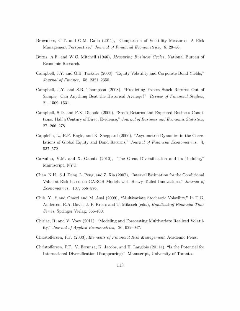
Brownlees, C.T. and G.M. Gallo (2011), “Comparison of Volatility Measures: A Risk

Management Perspective,” Journal of Financial Econometrics, 8, 29–56.

Burns, A.F. and W.C. Mitchell (1946), Measuring Business Cycles, National Bureau of

Economic Research.

Campbell, J.Y. and G.B. Tacksler (2003), “Equity Volatility and Corporate Bond Yields,”

Journal of Finance, 58, 2321–2350.

Campbell, J.Y. and S.B. Thompson (2008), “Predicting Excess Stock Returns Out of

Sample: Can Anything Beat the Historical Average?” Review of Financial Studies,

21, 1509–1531.

Campbell, S.D. and F.X. Diebold (2009), “Stock Returns and Expected Business Condi-

tions: Half a Century of Direct Evidence,” Journal of Business and Economic Statistics,

27, 266–278.

Cappiello, L., R.F. Engle, and K. Sheppard (2006), “Asymmetric Dynamics in the Corre-

lations of Global Equity and Bond Returns,” Journal of Financial Econometrics, 4,

537–572.

Carvalho, V.M. and X. Gabaix (2010), “The Great Diversification and its Undoing,”

Manuscript, NYU.

Chan, N.H., S.J. Deng, L. Peng, and Z. Xia (2007), “Interval Estimation for the Conditional

Value-at-Risk based on GARCH Models with Heavy Tailed Innovations,” Journal of

Econometrics, 137, 556–576.

Chib, Y., S.and Omori and M. Asai (2009), “Multivariate Stochastic Volatility,” In T.G.

Andersen, R.A. Davis, J.-P. Kreiss and T. Mikosch (eds.), Handbook of Financial Time

Series, Springer Verlag, 365-400.

Chiriac, R. and V. Voev (2011), “Modeling and Forecasting Multivariate Realized Volatil-

ity,” Journal of Applied Econometrics, 26, 922–947.

Christoffersen, P.F. (2003), Elements of Financial Risk Management, Academic Press.

Christoffersen, P.F., V. Errunza, K. Jacobs, and H. Langlois (2011a), “Is the Potential for

International Diversification Disappearing?” Manuscript, University of Toronto.

113

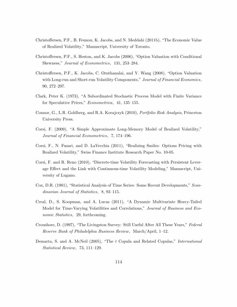
Christoffersen, P.F., B. Feunou, K. Jacobs, and N. Meddahi (2011b), “The Economic Value

of Realized Volatility,” Manuscript, University of Toronto.

Christoffersen, P.F., S. Heston, and K. Jacobs (2006), “Option Valuation with Conditional

Skewness,” Journal of Econometrics, 131, 253–284.

Christoffersen, P.F., K. Jacobs, C. Ornthanalai, and Y. Wang (2008), “Option Valuation

with Long-run and Short-run Volatility Components,” Journal of Financial Economics,

90, 272–297.

Clark, Peter K. (1973), “A Subordinated Stochastic Process Model with Finite Variance

for Speculative Prices,” Econometrica, 41, 135–155.

Connor, G., L.R. Goldberg, and R.A. Korajczyk (2010), Portfolio Risk Analysis, Princeton

University Press.

Corsi, F. (2009), “A Simple Approximate Long-Memory Model of Realized Volatility,”

Journal of Financial Econometrics, 7, 174–196.

Corsi, F., N. Fusari, and D. LaVecchia (2011), “Realizing Smiles: Options Pricing with

Realized Volatility,” Swiss Finance Institute Research Paper No. 10-05.

Corsi, F. and R. Reno (2010), “Discrete-time Volatility Forecasting with Persistent Lever-

age Effect and the Link with Continuous-time Volatility Modeling,” Manuscript, Uni-

versity of Lugano.

Cox, D.R. (1981), “Statistical Analysis of Time Series: Some Recent Developments,” Scan-

dinavian Journal of Statistics, 8, 93–115.

Creal, D., S. Koopman, and A. Lucas (2011), “A Dynamic Multivariate Heavy-Tailed

Model for Time-Varying Volatilities and Correlations,” Journal of Business and Eco-

nomic Statistics, 29, forthcoming.

Croushore, D. (1997), “The Livingston Survey: Still Useful After All These Years,” Federal

Reserve Bank of Philadelphia Business Review , March/April, 1–12.

Demarta, S. and A. McNeil (2005), “The t Copula and Related Copulas,” International

Statistical Review , 73, 111–129.

114

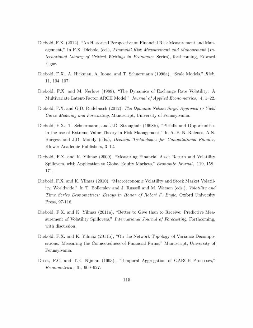
Diebold, F.X. (2012), “An Historical Perspective on Financial Risk Measurement and Man-

agement,” In F.X. Diebold (ed.), Financial Risk Measurement and Management (In-

ternational Library of Critical Writings in Economics Series), forthcoming, Edward

Elgar.

Diebold, F.X., A. Hickman, A. Inoue, and T. Schuermann (1998a), “Scale Models,” Risk ,

11, 104–107.

Diebold, F.X. and M. Nerlove (1989), “The Dynamics of Exchange Rate Volatility: A

Multivariate Latent-Factor ARCH Model,” Journal of Applied Econometrics, 4, 1–22.

Diebold, F.X. and G.D. Rudebusch (2012), The Dynamic Nelson-Siegel Approach to Yield

Curve Modeling and Forecasting, Manuscript, University of Pennsylvania.

Diebold, F.X., T. Schuermann, and J.D. Stroughair (1998b), “Pitfalls and Opportunities

in the use of Extreme Value Theory in Risk Management,” In A.-P. N. Refenes, A.N.

Burgess and J.D. Moody (eds.), Decision Technologies for Computational Finance,

Kluwer Academic Publishers, 3–12.

Diebold, F.X. and K. Yilmaz (2009), “Measuring Financial Asset Return and Volatility

Spillovers, with Application to Global Equity Markets,” Economic Journal , 119, 158–

171.

Diebold, F.X. and K. Yilmaz (2010), “Macroeconomic Volatility and Stock Market Volatil-

ity, Worldwide,” In T. Bollerslev and J. Russell and M. Watson (eds.), Volatility and

Time Series Econometrics: Essays in Honor of Robert F. Engle, Oxford University

Press, 97-116.

Diebold, F.X. and K. Yilmaz (2011a), “Better to Give than to Receive: Predictive Mea-

surement of Volatility Spillovers,” International Journal of Forecasting, Forthcoming,

with discussion.

Diebold, F.X. and K. Yilmaz (2011b), “On the Network Topology of Variance Decompo-

sitions: Measuring the Connectedness of Financial Firms,” Manuscript, University of

Pennsylvania.

Drost, F.C. and T.E. Nijman (1993), “Temporal Aggregation of GARCH Processes,”

Econometrica, 61, 909–927.

115

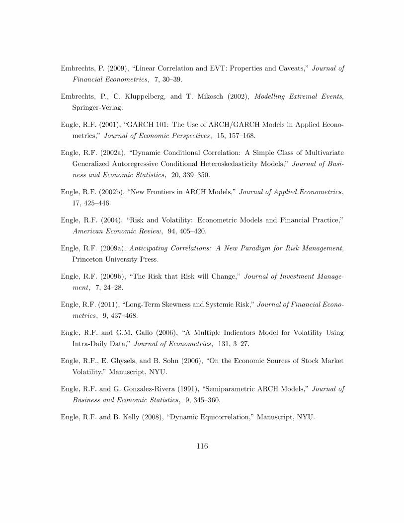
Embrechts, P. (2009), “Linear Correlation and EVT: Properties and Caveats,” Journal of

Financial Econometrics, 7, 30–39.

Embrechts, P., C. Kluppelberg, and T. Mikosch (2002), Modelling Extremal Events,

Springer-Verlag.

Engle, R.F. (2001), “GARCH 101: The Use of ARCH/GARCH Models in Applied Econo-

metrics,” Journal of Economic Perspectives, 15, 157–168.

Engle, R.F. (2002a), “Dynamic Conditional Correlation: A Simple Class of Multivariate

Generalized Autoregressive Conditional Heteroskedasticity Models,” Journal of Busi-

ness and Economic Statistics, 20, 339–350.

Engle, R.F. (2002b), “New Frontiers in ARCH Models,” Journal of Applied Econometrics,

17, 425–446.

Engle, R.F. (2004), “Risk and Volatility: Econometric Models and Financial Practice,”

American Economic Review , 94, 405–420.

Engle, R.F. (2009a), Anticipating Correlations: A New Paradigm for Risk Management,

Princeton University Press.

Engle, R.F. (2009b), “The Risk that Risk will Change,” Journal of Investment Manage-

ment , 7, 24–28.

Engle, R.F. (2011), “Long-Term Skewness and Systemic Risk,” Journal of Financial Econo-

metrics, 9, 437–468.

Engle, R.F. and G.M. Gallo (2006), “A Multiple Indicators Model for Volatility Using

Intra-Daily Data,” Journal of Econometrics, 131, 3–27.

Engle, R.F., E. Ghysels, and B. Sohn (2006), “On the Economic Sources of Stock Market

Volatility,” Manuscript, NYU.

Engle, R.F. and G. Gonzalez-Rivera (1991), “Semiparametric ARCH Models,” Journal of

Business and Economic Statistics, 9, 345–360.

Engle, R.F. and B. Kelly (2008), “Dynamic Equicorrelation,” Manuscript, NYU.

116

Engle, R.F. and G.G.J. Lee (1999), “A Permanent and Transitory Component Model of

Stock Return Volatility,” In R.F. Engle and H. White (eds.), Cointegration, Causality,

and Forecasting: A Festschrift in Honor of Clive W.J. Granger. Oxford University

Press, 475-497.

Engle, R.F., D.M. Lilien, and R.P. Robbins (1987), “Estimating Time-Varying Risk Premia

in the Term Structure: The ARCH-M Model,” Econometrica, 55, 391–407.

Engle, R.F. and J. Mezrich (1996), “GARCH for Groups,” Risk , 9, 36–40.

Engle, R.F. and V.K. Ng (1993), “Measuring and Testing the Impact of News on Volatility,”

Journal of Finance, 48, 1749–1778.

Engle, R.F., V.K. Ng, and M. Rothschild (1990), “Asset Pricing with a Factor-ARCH

Covariance Structure,” Journal of Econometrics, 45, 213–238.

Engle, R.F. and J.G. Rangel (2008), “The Spline GARCH Model for Unconditional Volatil-

ity and Its Global Macroeconomic Causes,” Review of Financial Studies, 21, 1187–

1222.

Engle, R.F. and J.G. Rangel (2011), “The Factor-Spline-GARCH Model for High and Low

Frequency Correlations,” Journal of Business and Economic Statistics, 29, in press.

Engle, R.F., N. Shephard, and K. Sheppard (2008), “Fitting Vast Dimensional Time-

Varying Covariance Models,” Manuscript, NYU.

Epps, T.W. (1979), “Comovement in Stock Prices in the Very Short Run,” Journal of the

American Statistical Association, 74, 291–298.

Epstein, L. and S.E. Zin (1989), “Substitution, Risk Aversion and the Temporal Behavior

of Consumption and Asset Returns: A Theoretical Framework,” Econometrica, 57,

937–969.

Fama, E.F. (1965), “The Behavior of Stock-Market Prices,” Journal of Business, 38,

34–105.

Fama, E.F. (1990), “Stock Returns, Expected Returns, and Real Activity,” Journal of

Finance, 45, 1089–1108.

117

Fama, E.F. and K.R. French (1989), “Business Conditions and Expected Returns on Stocks

and Bonds,” Journal of Financial Economics, 25, 23–49.

Fan, J., Y. Fan, and J. Lv (2008), “High Dimensional Covariance Matrix Estimation Using

a Factor Model,” Journal of Econometrics, 147, 186–197.

Fan, J., Y. Liao, and M. Mincheva (2011), “High Dimensional Covariance Matrix Estima-

tion in Approximate Factor Models,” Manuscript, Princeton University.

Fernandez, C. and M.F.J. Steel (1998), “On Bayesian Modeling of Fat Tails and Skewness.”

Journal of the American Statistical Association, 93, 359–371.

Fernandez-Villaverde, J., P.A. Guerron-Quintana, J. Rubio-Ramırez, and M. Uribe (2011),

“Risk Matters: The Real Effects of Volatility Shocks,” American Economic Review,

forthcoming.

Fernandez-Villaverde, J. and J.F. Rubio-Ramırez (2011), “Macroeconomics and Volatility:

Data, Models, and Estimation,” In D. Acemoglu, M. Arellano and E. Deckel (eds.),

Advances in Economics and Econometrics: Theory and Applications, Tenth World

Congress of the Econometric Society, Cambridge University Press, Forthcoming.

Fleming, J., C. Kirby, and B. Ostdiek (2003), “The Economic Value of Volatility Timing

using Realized Volatility,” Journal of Financial Economics, 63, 473–509.

Follmer, H. and A. Schied (2002), “Convex Measures of Risk and Trading Constraints,”

Finance and Stochastics, 6, 429–447.

Forsberg, L. and T. Bollerslev (2002), “Bridging the Gap Between the Distribution of Re-

alized (ECU) Volatility and ARCH Modeling (of the Euro): The GARCH-NIG Model,”

Journal Applied Econometrics, 17, 535–548.

Gallant, A.R., C.T. Hsu, and G. Tauchen (1999), “Using Daily Range Data to Calibrate

Volatility Diffusions and Extract the Forward Integrated Variance,” Review of Eco-

nomics and Statistics, 81, 617–631.

Garcia, R., E. Renault, and G. Tsafack (2007), “Proper Conditioning for Coherent VaR in

Portfolio Management,” Management Science, 53, 483–494.

118

Glasserman, P., P. Heidelberger, and P. Shahabuddin (2002), “Portfolio Value-at-Risk with

Heavy-Tailed Risk Factors,” Mathematical Finance, 12, 239–269.

Glosten, L.R., R. Jagannathan, and D.E. Runkle (1993), “On the Relation Between the

Expected Value and the Volatility of the Nominal Excess Return on Stocks,” Journal

of Finance, 48, 1779–1801.

Goetzman, W.N., A. Watanabe, and M. Watanabe (2009), “Investor Expectations, Busi-

ness Conditions, and the Pricing of Beta-Instability Risk,” Manuscript, Yale University.

Golosnoy, V., B. Glibisch, and R. Liesenfeld (2010), “The Conditional Autoregressive

Wishart Model for Multivariate Stock Market Volatility,” Manuscript, Christian-

Albrechts-University of Kiel.

Gourieroux, C., J. Jasiak, and R. Sufana (2009), “The Wishart Autoregressive Process of

Multivariate Stochastic Volatility,” Journal of Econometrics, 150, 167–181.

Granger, C. W. J. (1980), “Long Memory Relationships and the Aggregation of Dynamic

Models,” Journal of Econometrics, 14, 227–238.

Guidolin, M. and A. Timmermann (2006), “Term Structure of Risk Under Alternative

Econometric Specifications,” Journal of Econometrics, 131, 285–308.

Hafner, C. and H. Manner (2011), “Dynamic Stochastic Copula Models: Estimation, In-

ference and Applications,” Journal of Applied Econometrics, forthcoming.

Hamilton, J.D. and G. Lin (1996), “Stock Market Volatility and the Business Cycle,”

Journal of Applied Econometrics, 11, 573–593.

Hansen, B.E. (1994), “Autoregressive Conditional Density Estimation,” International Eco-

nomic Review , 35, 705–730.

Hansen, P.R., Z. Huang, and H. Shek (2010a), “Realized GARCH: A Complete Model

of Returns and Realized Measures of Volatility,” Journal of Applied Econometrics,

forthcoming.

Hansen, P.R. and A. Lunde (2005), “A Realized Variance for the Whole Day Based on

Intermittent High-Frequency Data,” Journal of Financial Econometrics, 3, 525–554.

119

Hansen, P.R. and A. Lunde (2006), “Realized Variance and Market Microstructure Noise,”

Journal of Business and Economic Statistics, 24, 127–161.

Hansen, P.R., A. Lunde, and V. Voev (2010b), “Realized Beta GARCH: A Multivariate

GARCH Model with Realized Measures of Volatility and CoVolatility,” Manuscript,

University of Aarhus.

Harvey, A., E. Ruiz, and E. Sentana (1992), “Unobserved Component Time Series Models

with ARCH Disturbances,” Journal of Econometrics, 52, 129–157.

Harvey, A.C. (1989), Forecasting, Structural Time Series Models and the Kalman Filter,

Cambridge University Press.

Hautsch, N., L.M. Kyj, and R.C.A. Oomen (2011), “A Blocking and Regularization Ap-

proach to High Dimensional Realized Covariance Estimation,” Journal of Applied

Econometrics, forthcoming.

Heston, S.L. and S. Nandi (2000), “A Closed-Form GARCH Option Valuation Model,”

Review of Financial Studies, 13, 585–625.

Hull, J. and A. White (1998), “Incorporating Volatility Updating into the Historical Sim-

ulation Method for Value-at-Risk,” Journal of Risk , 1, 5–19.

Jacod, J., Y. Li, P. Mykland, M. Podolskij, and M. Vetter (2009), “Microstructure Noise

in the Continuous Case: The Pre-Averaging Approach,” Stochastic Processes and their

Applications, 119, 2249–2276.

Jin, X. and J.M. Maheu (2010), “Modeling Realized Covariances and Returns,”

Manuscript, University of Toronto.

Jondeau, E. and M. Rockinger (2006), “The Copula-GARCH Model of Conditional Depen-

dencies: An International Stock Market Application,” Journal of International Money

and Finance, 25, 827–853.

Jorion, P. (2007), Value at Risk: The New Benchmark for Managing Financial Risk,

McGraw-Hill, third edition.

Kawakatsu, H. (2006), “Matrix Exponential GARCH,” Journal of Econometrics, 134,

95–128.

120

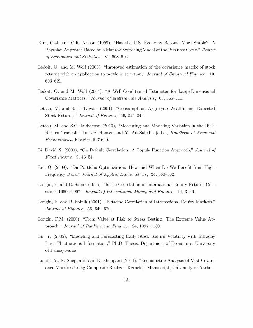
Kim, C.-J. and C.R. Nelson (1999), “Has the U.S. Economy Become More Stable? A

Bayesian Approach Based on a Markov-Switching Model of the Business Cycle,” Review

of Economics and Statistics, 81, 608–616.

Ledoit, O. and M. Wolf (2003), “Improved estimation of the covariance matrix of stock

returns with an application to portfolio selection,” Journal of Empirical Finance, 10,

603–621.

Ledoit, O. and M. Wolf (2004), “A Well-Conditioned Estimator for Large-Dimensional

Covariance Matrices,” Journal of Multivariate Analysis, 68, 365–411.

Lettau, M. and S. Ludvigson (2001), “Consumption, Aggregate Wealth, and Expected

Stock Returns,” Journal of Finance, 56, 815–849.

Lettau, M. and S.C. Ludvigson (2010), “Measuring and Modeling Variation in the Risk-

Return Tradeoff,” In L.P. Hansen and Y. Aıt-Sahalia (eds.), Handbook of Financial

Econometrics, Elsevier, 617-690.

Li, David X. (2000), “On Default Correlation: A Copula Function Approach,” Journal of

Fixed Income, 9, 43–54.

Liu, Q. (2009), “On Portfolio Optimization: How and When Do We Benefit from High-

Frequency Data,” Journal of Applied Econometrics, 24, 560–582.

Longin, F. and B. Solnik (1995), “Is the Correlation in International Equity Returns Con-

stant: 1960-1990?” Journal of International Money and Finance, 14, 3–26.

Longin, F. and B. Solnik (2001), “Extreme Correlation of International Equity Markets,”

Journal of Finance, 56, 649–676.

Longin, F.M. (2000), “From Value at Risk to Stress Testing: The Extreme Value Ap-

proach,” Journal of Banking and Finance, 24, 1097–1130.

Lu, Y. (2005), “Modeling and Forecasting Daily Stock Return Volatility with Intraday

Price Fluctuations Information,” Ph.D. Thesis, Department of Economics, University

of Pennsylvania.

Lunde, A., N. Shephard, and K. Sheppard (2011), “Econometric Analysis of Vast Covari-

ance Matrices Using Composite Realized Kernels,” Manuscript, University of Aarhus.

121

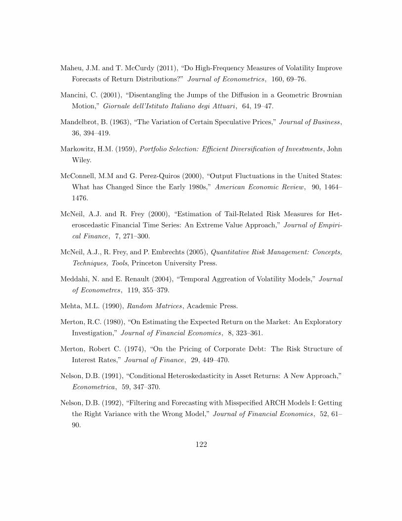
Maheu, J.M. and T. McCurdy (2011), “Do High-Frequency Measures of Volatility Improve

Forecasts of Return Distributions?” Journal of Econometrics, 160, 69–76.

Mancini, C. (2001), “Disentangling the Jumps of the Diffusion in a Geometric Brownian

Motion,” Giornale dell’Istituto Italiano degi Attuari , 64, 19–47.

Mandelbrot, B. (1963), “The Variation of Certain Speculative Prices,” Journal of Business,

36, 394–419.

Markowitz, H.M. (1959), Portfolio Selection: Efficient Diversification of Investments, John

Wiley.

McConnell, M.M and G. Perez-Quiros (2000), “Output Fluctuations in the United States:

What has Changed Since the Early 1980s,” American Economic Review , 90, 1464–

1476.

McNeil, A.J. and R. Frey (2000), “Estimation of Tail-Related Risk Measures for Het-

eroscedastic Financial Time Series: An Extreme Value Approach,” Journal of Empiri-

cal Finance, 7, 271–300.

McNeil, A.J., R. Frey, and P. Embrechts (2005), Quantitative Risk Management: Concepts,

Techniques, Tools, Princeton University Press.

Meddahi, N. and E. Renault (2004), “Temporal Aggreation of Volatility Models,” Journal

of Econometrcs, 119, 355–379.

Mehta, M.L. (1990), Random Matrices, Academic Press.

Merton, R.C. (1980), “On Estimating the Expected Return on the Market: An Exploratory

Investigation,” Journal of Financial Economics, 8, 323–361.

Merton, Robert C. (1974), “On the Pricing of Corporate Debt: The Risk Structure of

Interest Rates,” Journal of Finance, 29, 449–470.

Nelson, D.B. (1991), “Conditional Heteroskedasticity in Asset Returns: A New Approach,”

Econometrica, 59, 347–370.

Nelson, D.B. (1992), “Filtering and Forecasting with Misspecified ARCH Models I: Getting

the Right Variance with the Wrong Model,” Journal of Financial Economics, 52, 61–

90.

122

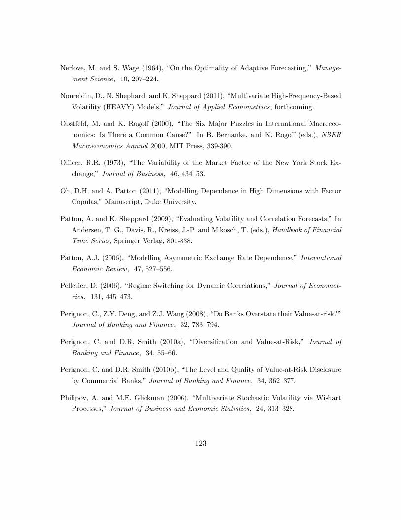
Nerlove, M. and S. Wage (1964), “On the Optimality of Adaptive Forecasting,” Manage-

ment Science, 10, 207–224.

Noureldin, D., N. Shephard, and K. Sheppard (2011), “Multivariate High-Frequency-Based

Volatility (HEAVY) Models,” Journal of Applied Econometrics, forthcoming.

Obstfeld, M. and K. Rogoff (2000), “The Six Major Puzzles in International Macroeco-

nomics: Is There a Common Cause?” In B. Bernanke, and K. Rogoff (eds.), NBER

Macroeconomics Annual 2000, MIT Press, 339-390.

Officer, R.R. (1973), “The Variability of the Market Factor of the New York Stock Ex-

change,” Journal of Business, 46, 434–53.

Oh, D.H. and A. Patton (2011), “Modelling Dependence in High Dimensions with Factor

Copulas,” Manuscript, Duke University.

Patton, A. and K. Sheppard (2009), “Evaluating Volatility and Correlation Forecasts,” In

Andersen, T. G., Davis, R., Kreiss, J.-P. and Mikosch, T. (eds.), Handbook of Financial

Time Series, Springer Verlag, 801-838.

Patton, A.J. (2006), “Modelling Asymmetric Exchange Rate Dependence,” International

Economic Review , 47, 527–556.

Pelletier, D. (2006), “Regime Switching for Dynamic Correlations,” Journal of Economet-

rics, 131, 445–473.

Perignon, C., Z.Y. Deng, and Z.J. Wang (2008), “Do Banks Overstate their Value-at-risk?”

Journal of Banking and Finance, 32, 783–794.

Perignon, C. and D.R. Smith (2010a), “Diversification and Value-at-Risk,” Journal of

Banking and Finance, 34, 55–66.

Perignon, C. and D.R. Smith (2010b), “The Level and Quality of Value-at-Risk Disclosure

by Commercial Banks,” Journal of Banking and Finance, 34, 362–377.

Philipov, A. and M.E. Glickman (2006), “Multivariate Stochastic Volatility via Wishart

Processes,” Journal of Business and Economic Statistics, 24, 313–328.

123

Poon, S.H., M. Rockinger, and J. Tawn (2004), “Extreme Value Dependence in Finan-

cial Markets: Diagnostics, Models, and Financial Implications,” Review of Financial

Studies, 17, 581–610.

Pritsker, M. (2006), “The Hidden Dangers of Historical Simulation,” Journal of Banking

and Finance, 30, 561–582.

Rosenberg, J. V. and T. Schuermann (2006), “A General Approach to Integrated Risk

Management with Skewed, Fat-Tailed Risks,” Journal of Financial Economics, 79,

569–614.

Rosenow, B. (2008), “Determining the Optimal Dimensionality of Multivariate Volatility

Models with Tools from Random Matrix Theory,” Journal of Economic Dynamics and

Control , 32, 279–302.

Schwert, G.W. (1989), “Why Does Stock Market Volatility Change Over Time?” Journal

of Finance, 44, 1115–1153.

Shephard, N. and K. Sheppard (2010), “Realising the Future: Forecasting with High-

Frequency-Based Volatility (HEAVY) Models,” Journal of Applied Econometrics, 25,

197–231.

Shiller, R.J. (1981), “Do Stock Prices Move Too Much to be Justified by Subsequent

Changes in Dividends?” American Economic Review , 71, 421–436.

Sizova, N. (2011), “Integrated Variance Forecasting: Model Based vs. Reduced Form,”

Journal of Econometrics, 162, 294–311.

Stentoft, L. (2008), “Option Pricing Using Realized Volatility,” Manuscript, University of

Aarhus.

Stock, J.H. and M.W. Watson (2002), “Has the Business Cycle Changed and Why?” In

M. Gertler and K. Rogoff (eds.), NBER Macroeconomics Annual, MIT Press, 159-218.

Stulz, R.M. (2002), “Risk Management and Derivatives,” South-Western.

Stulz, R.M. (2008), “Risk Management Failures: What are They and When do They

Happen?” Journal of Applied Corporate Finance, 20, 58–67.

124

Tola, V., F. Lillo, M. Gallegati, and R.N. Mantegna (2008), “Cluster Analysis for Portfolio

Optimization,” Journal of Economic Dynamics and Control , 32, 235–258.

Tse, Y.K. and A.K.C. Tsui (2002), “A Multivariate Generalized Autoreressive Conditional

Heteroskedasticity Model with Time-varying Correlations,” Journal of Business and

Economic Statistics, 20, 351–362.

Varneskov, R.T. and V. Voev (2010), “The Role of Realized Ex-Post Covariance Measures

and Dynamic Model Choice on the Quality of Covariance Forecasts,” Manuscript, Uni-

versity of Aarhus.

Visser, M.P. (2011), “GARCH Parameter Estimation Using High-Frequency Data,” Jour-

nal of Financial Econometrics, 9, 162–197.

Wang, Y. and J. Zou (2010), “Vast Volatility Matrix Estimation for High-Frequency Fi-

nancial Data,” Annals of Statistics, 38, 943–978.

White, H., T.-H. Kim, and S. Manganelli (2010), “VAR for VaR: Measuring Systemic Risk

Using Multivariate Regression Quantiles,” Manuscript, UCSD.

Whitelaw, R.F. (2000), “Stock Market Risk and Return: An Equilibrium Approach,”

Review of Financial Studies, 13, 521–547.

Zhou, B. (1996), “High-Frequency Data and Volatility in Foreign-Exchange Rates,” Journal

of Business and Economic Statistics, 14, 45–52.

Zumbach, G. (2006), “A Gentle Introduction to the RM 2006 Methodology,” Mannscript,

RiskMetrics Group.

125