Sovereign Risk and Financial Risk

Simon Gilchrist1 Bin Wei2 Vivian Yue3 Egon Zakrajšek4

1New York University and NBER

2Federal Reserve Bank of Atlanta

3Emory University, NBER and CEPR

4Bank of International Settlement and CEPR

June 2021The views expressed herein are those of the authors and do not necessarily reflect the views of the Federal

Reserve System or Bank of International Settlement.

Sovereign Debt and Default Risk

I Countries borrow on sovereign debt market

I Recurrent sovereign debt crises

I Country spreads on risky sovereign debt

I Question: how does global financial risk affect sovereign risk?

Literature on sovereign default and financial risk

I Risk premia on sovereign debtI Borri and Verdelhan (2011), Lizarazo (2013), Bai, Kehoe and

Perri (2019), Morelli, Ottonello and Perez (2019)

I Impact of global shocks on sovereign spreadsI Uribe and Yue (2006), Akinci (2013), Gilchrist, Yue and

Zakrajsek (2019)I Longstaff, Pan, Pederson and Singleton (2011), Ang and

Longstaff (2013)

I Global financial cyclesI Rey (2013), Kalemli-Ozcan (2019), Miranda-Agrippino and

Rey (2020)

This paper

I Construct an extensive micro-level dataset of sovereign bondspreads

I Examine the extent to which movements in sovereign bondand CDS spreads are driven by global financial risk factors.

I Explore the theoretical linkages between total intermediationcapacity of the financial sector and sovereign bond risk premia

Measuring Sovereign Risk

I Sovereign CDS Spreads (derivatives)I 15 developing countriesI Jan 2003-Oct 2020I Decompose the CDS spreads into their default and

risk-premium components.I Sovereign Bond Spreads (cash)

I Dollar-denominated bonds traded in the secondary market.I Jan1995–Oct2020; 1,794 securities; 53 countries;

94,521 bond/month observationsI Construct micro-level credit spreads using synthetic risk-free

securities priced off zero-coupon U.S. Treasuries:

P fit [k] =

S∑s=1

C(s)D(ts); D(t) = exp[−r ft t]

Sovereign Bond Characteristics

Bond Characteristic Mean StdDev Min Median Max

No. of bonds per country/month 10.3 46.0 1 4 865Term to maturity (years) 8.5 8.4 0.16 6.4 100Yield to maturity (bps.) 375 300 0.09 303 2,309Credit spread (bps.) 231 225 0.01 165 1,998

Percentage of IG bonds 69%

Sovereign CDS Spreads

2003Jan 2006Jul 2010Feb 2013Sep 2017Apr 2020Oct0

100

200

300

400

500

600

700

5-year CDS Premium

Default Component

Sovereign Bond Spreads

1995 2000 2005 2010 2015 20200

100

200

300

400

500

600

1995 2000 2005 2010 2015 20200

200

400

600

800

1000

1200

Measuring Financial Sector Risk

I Excess Bond Premium (EBP): an indicator of financialdistress based on U.S. nonfinancial corporate bond spreads:(Measured as the difference between average U.S. corporate bond spread andaverage expected default risk Gilchrist & Zakrajšek [2012])

I Global Financial Cycle factor (GFC): an indicator of aggregatevolatility or aggregate risk aversion in financial markets.(Measured as the global factor in world risky assets prices. Miranda-Agrippino &Rey [2020] )

I VIX is an alternative measure of global financial risk due toaggregate volatility.

Measures of Global Financial Risk

1990Jan 1996Mar 2002May 2008Aug 2014Oct 2020Dec-3

-2

-1

0

1

2

3

4

0

10

20

30

40

50

60

EBP

GFC

VIX

Global Risk Factors and Sovereign CDS Spreads

CDS Spread Default Component Risk-Premium Component(1) (2) (3) (4) (5) (6) (7) (8) (9) (10) (11) (12)

EBP22.04∗ −5.23 11.26∗∗ 2.57 10.78 −7.80(11.78) (14.53) (3.79) (2.29) (9.72) (12.95)

GFC 38.10∗∗∗ 38.67∗∗∗ 9.33∗∗∗ 7.79∗∗ 28.78∗∗∗ 30.87∗∗(9.39) (12.31) (2.81) (2.80) (8.83) (11.33)

VIX 1.59∗∗ 0.24 0.62∗ 0.50 0.96∗ −0.26(0.72) (1.12) (0.29) (0.39) (0.51) (0.81)

R2 0.40 0.44 0.40 0.44 0.65 0.67 0.64 0.67 0.29 0.33 0.29 0.33N 2,924 2,672 2,924 2,672 2,924 2,672 2,924 2,672 2,924 2,672 2,924 2,672

Note: Standard errors are clustered in bond and date dimensions. * p < 0.10, ** p < 0.05, *** p < 0.01Other global factors: SP500 return, 2-year real rate, term spreadLocal factors: stock returns and realized vol, FX returns and realized vol

Global Risk Factors and Sovereign Bond Spreads

Investment Grade Speculative Grade(1) (2) (3) (4) (5) (6) (7) (8)

EBP 0.13∗∗∗ 0.07 0.52∗∗∗ 0.11(0.05) (0.05) (0.11) (0.14)

GFC 0.14∗∗∗ 0.12∗∗∗ 0.81∗∗∗ 0.83∗∗∗(0.03) (0.04) (0.09) (0.09)

VIX 0.01∗∗∗ −0.00 0.05∗∗∗ −0.02(0.00) (0.00) (0.01) (0.01)

R2 0.73 0.73 0.72 0.73 0.65 0.69 0.65 0.69Obs. 65,116 65,116 65,116 65,116 21,605 21,605 21,605 21,605

Note: Standard errors are clustered in bond and date dimensions. * p < 0.10, ** p < 0.05, *** p < 0.01Other global factors: SP500 return, 2-year real rate, term spread

Local factors: stock returns and realized vol, FX returns and realized volBond controls: coupon rate, coupon freq, time to maturity, par value

Persistence of Global Factors’ Effects

CDS Premium Default Risk Risk Premium1-month 6-month 1-month 6-month 1-month 6-month

EBP −1.92 35.35∗ 2.94 13.51∗∗ −4.86 21.84(13.99) (17.92) (2.49) (5.48) (12.27) (13.33)

GFC 31.16∗∗ −9.00 5.93∗∗ −5.12 25.24∗∗ −3.88(11.64) (10.74) (2.64) (3.02) (10.54) (8.36)

VIX −0.11 −1.83 0.41 −0.34 −0.52 −1.49(1.22) (1.18) (0.44) (0.46) (0.86) (0.85)

R2 0.45 0.38 0.67 0.63 0.34 0.27Obs. 2,668 2,663 2,668 2,663 2,668 2,663

Note: Standard errors are clustered in bond and date dimensions. * p < 0.10, ** p < 0.05, *** p < 0.01Other global factors: SP500 return, 2-year real rate, term spread

Local factors: stock returns and realized vol, FX returns and realized vol

Persistence of Global Factors’ Effects

Lag(months) 1 2 3 4 5 6 9 12 18

Panel A: Investment GradeEBP 0.06 0.11 0.15∗ 0.23∗∗∗ 0.26∗∗∗ 0.30∗∗∗ 0.23∗∗∗ 0.26∗∗∗ −0.05

(0.06) (0.07) (0.08) (0.08) (0.08) (0.07) (0.07) (0.06) (0.07)GFC 0.07∗ 0.01 −0.05 −0.10∗∗ −0.14∗∗∗ −0.18∗∗∗ −0.27∗∗∗ −0.28∗∗∗ −0.18∗∗∗

(0.04) (0.04) (0.04) (0.05) (0.05) (0.05) (0.06) (0.06) (0.05)VIX 0.00 0.00 −0.00 −0.00 −0.01 −0.01 0.01 0.01 0.03∗∗∗

(0.01) (0.01) (0.01) (0.01) (0.01) (0.01) (0.01) (0.01) (0.01)

Panel B: Speculative GradeEBP 0.22 0.41∗∗ 0.47∗∗∗ 0.53∗∗∗ 0.56∗∗∗ 0.64∗∗∗ 0.61∗∗∗ 0.61∗∗∗ 0.28∗

(0.15) (0.16) (0.17) (0.17) (0.16) (0.16) (0.18) (0.16) (0.16)GFC 0.72∗∗∗ 0.57∗∗∗ 0.46∗∗∗ 0.33∗∗∗ 0.24∗∗ 0.16 −0.02 −0.18 −0.41∗∗∗

(0.09) (0.10) (0.11) (0.11) (0.11) (0.12) (0.12) (0.13) (0.10VIX −0.03∗ −0.04∗∗ −0.04∗∗ −0.04∗∗ −0.04∗∗ −0.04∗∗ −0.02 −0.01 0.05∗∗∗

(0.01) (0.02) (0.02) (0.02) (0.02) (0.02) (0.02) (0.02) (0.01)

Note: Standard errors are clustered in bond and date dimensions. * p < 0.10, ** p < 0.05, *** p < 0.01

Impact of Global Financial Risk on Sovereign Spreads

I Local projection regression

sk,i ,t+j = b0,i +p

∑q=1

βs,q,jsi ,t−j +p

∑q=1

βx ,q,jxt−q +p

∑q=1

βy ,q,jyi ,t−q

+ βz ,k,tzk,i ,t + βx ,j xt + βy ,j yi ,t + eit

I xt = global factors(real yield on U.S. 2-year treasury bond, slope of U.S. yield curve,S&P 500 return, VIX, EBP and GFC)

I yit = country-specific factors(stock returns, FX returns, realized equity volatility)

I zit [k] = bond-specific control variables(duration, par amount, age, coupon, coupon freq.)

Impulse Response of Sovereign Spreads to Global FinancialRisk

I Local projection regression

sk,i ,t+j = b0,i +p

∑q=1

βs,q,jsi ,t−j +p

∑q=1

βx ,q,jxt−q +p

∑q=1

βy ,q,jyi ,t−q

+ βz ,k,tzk,i ,t + βx ,j xt + βy ,j yi ,t + eit

I xt = shocks calculated as orthogonalized residuals obtainedfrom a regression of xt on six lags of xt . xt = normalized by itsstd. Cholesky decomposition with ordering of(real yield on U.S. 2-year treasury bond, slope of U.S. yield curve,S&P 500 return, VIX, EBP and GFC)

I βx ,j = estimated impulse response of the sovereign spread si ,tat horizon j to a one-standard deviation shock

I Alternative with EBP ordered last.

Implications of a Financial Sector Risk Shock

-.10

.1.2

3 6 9 12 15 18 21 24Response to EBP

IG Spread

-.10

.1.2

3 6 9 12 15 18 21 24Response to EBP

SG Spread-.1

0.1

.2

3 6 9 12 15 18 21 24Response to GFC

Order 1 Order 2

IG Spread

-.10

.1.2

3 6 9 12 15 18 21 24Response to GFC

SG Spread

Simple Model to Illustrate Empirical Results

I Introduce international financial intermediaries into a model ofsovereign debt

I Banks with Value-at-Risk rule and mean-variance investors(Shin (2012), Adrian and Shin (2011), Miranda-Agrippino andRey (2020))

Sovereign Borrowers

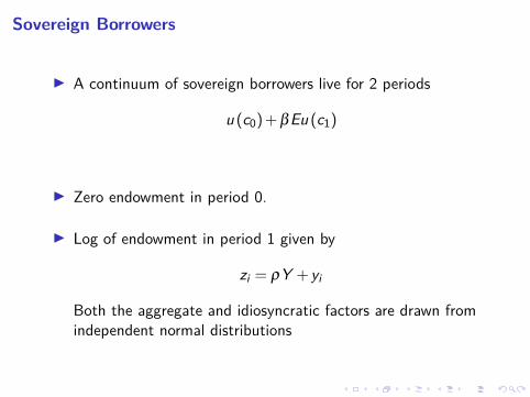
I A continuum of sovereign borrowers live for 2 periods

u (c0) + βEu (c1)

I Zero endowment in period 0.

I Log of endowment in period 1 given by

zi = ρY + yi

Both the aggregate and idiosyncratic factors are drawn fromindependent normal distributions

Sovereign Borrowers

I A continuum of sovereign borrowers live for 2 periods

u (c0) + βEu (c1)

I Zero endowment in period 0.

I Log of endowment in period 1 given by

zi = ρY + yi

Both the aggregate and idiosyncratic factors are drawn fromindependent normal distributions

Sovereign Default Risk

I Individual country borrows discount bond to smoothconsumption and can default

I If a country defaults, its income drops to (1−φ)exp(zi )

I The default cutoff z∗ is given by

z∗ = log

(bφ

)

I Demand for sovereign bond for each country:

maxb>0;

u (q (b)b) + β

[ ∫z∗ u (exp(z)−b)dP (z)

+∫ z∗ u ((1−φ)exp(z))dP (zi )

]

Sovereign Default Risk

I Individual country borrows discount bond to smoothconsumption and can default

I If a country defaults, its income drops to (1−φ)exp(zi )

I The default cutoff z∗ is given by

z∗ = log

(bφ

)

I Demand for sovereign bond for each country:

maxb>0;

u (q (b)b) + β

[ ∫z∗ u (exp(z)−b)dP (z)

+∫ z∗ u ((1−φ)exp(z))dP (zi )

]

Sovereign Default Risk

I Individual country borrows discount bond to smoothconsumption and can default

I If a country defaults, its income drops to (1−φ)exp(zi )

I The default cutoff z∗ is given by

z∗ = log

(bφ

)

I Demand for sovereign bond for each country:

maxb>0;

u (q (b)b) + β

[ ∫z∗ u (exp(z)−b)dP (z)

+∫ z∗ u ((1−φ)exp(z))dP (zi )

]

Financial Intermediaries

I FI takes equity E as given, lends out is q (b)Bb at time 0 andborrows L at r f .I Balance sheet identity is

qBb = E + L.

I Financial intermediaries (FI) diversify away idiosyncratic creditrisk.I Conditional on Y , sovereign defaults are independent

Financial Intermediaries

I FI takes equity E as given, lends out is q (b)Bb at time 0 andborrows L at r f .I Balance sheet identity is

qBb = E + L.

I Financial intermediaries (FI) diversify away idiosyncratic creditrisk.I Conditional on Y , sovereign defaults are independent

Value-at-Risk Rule

I As in Shin (2012), financial intermediaries are risk neutral andmaximize expected profit subject only to a Value-at-Risk(VaR) constraint that limits the probability of bank failureI FI limits insolvency probability to α

Pr (ω ≤ (1+ rf )L)≤ α

where ω is the value of the bank’s assets at date 1I Backbone of Basel capital requirement. [Danielsson, Shin and

Zigrand (2009), Adrian, Etula and Shin (2011), Miranda Agrippino and Rey(2013) for evidence and applications on capital flow and risk premium.]

Value-at-Risk Rule

I As in Shin (2012), financial intermediaries are risk neutral andmaximize expected profit subject only to a Value-at-Risk(VaR) constraint that limits the probability of bank failureI FI limits insolvency probability to α

Pr (ω ≤ (1+ rf )L)≤ α

where ω is the value of the bank’s assets at date 1I Backbone of Basel capital requirement. [Danielsson, Shin and

Zigrand (2009), Adrian, Etula and Shin (2011), Miranda Agrippino and Rey(2013) for evidence and applications on capital flow and risk premium.]

Supply of Intermediated Credit

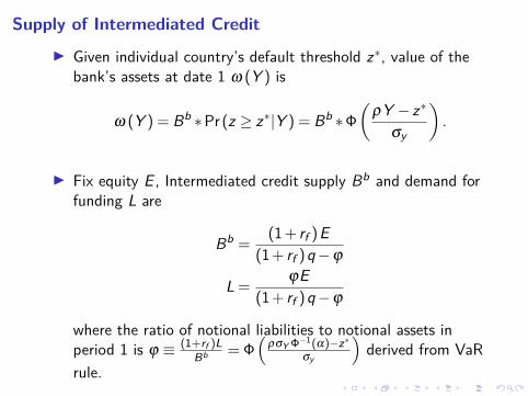
I Given individual country’s default threshold z∗, value of thebank’s assets at date 1 ω (Y ) is

ω (Y ) = Bb ∗Pr (z ≥ z∗|Y ) = Bb ∗Φ

(ρY − z∗

σy

).

I Fix equity E , Intermediated credit supply Bb and demand forfunding L are

Bb =(1+ rf )E

(1+ rf )q−ϕ

L =ϕE

(1+ rf )q−ϕ

where the ratio of notional liabilities to notional assets inperiod 1 is ϕ ≡ (1+rf )L

Bb = Φ(

ρσY Φ−1(α)−z∗σy

)derived from VaR

rule.

Supply of Intermediated Credit

I Given individual country’s default threshold z∗, value of thebank’s assets at date 1 ω (Y ) is

ω (Y ) = Bb ∗Pr (z ≥ z∗|Y ) = Bb ∗Φ

(ρY − z∗

σy

).

I Fix equity E , Intermediated credit supply Bb and demand forfunding L are

Bb =(1+ rf )E

(1+ rf )q−ϕ

L =ϕE

(1+ rf )q−ϕ

where the ratio of notional liabilities to notional assets inperiod 1 is ϕ ≡ (1+rf )L

Bb = Φ(

ρσY Φ−1(α)−z∗σy

)derived from VaR

rule.

Bond Investors

I Measure N of mean variance investors with risk aversionparameter σH purchase a diversified portfolio of sovereignbonds and deposits in FI.

I Supply for direct credit is

Bh = N (1−Ep)− (1+ rf )qσH ·var (p) 1

q

where the default probability p (Y ) = Φ(

z∗−ρYσy

)depends on

the aggregate shock Y , given sovereign’s default threshold z∗.

Bond Investors

I Measure N of mean variance investors with risk aversionparameter σH purchase a diversified portfolio of sovereignbonds and deposits in FI.

I Supply for direct credit is

Bh = N (1−Ep)− (1+ rf )qσH ·var (p) 1

q

where the default probability p (Y ) = Φ(

z∗−ρYσy

)depends on

the aggregate shock Y , given sovereign’s default threshold z∗.

Equilibrium

An equilibrium is{

q (b) ,b,Bb,Bh} such that

1. Given q (b), b solves the sovereign borrower’s problem. Thedefault cutoff z∗ characterizes the sovereign country’s defaultdecision.

2. Given q (b) and z∗, Bb is the bank credit supply.

3. Given q (b) and z∗, Bh is the households credit supply.

4. Sovereign debt market clears, such that

Bb + Bh = b

Parameters

Parameter EstimateσY 0.1σy 0.1ρ 0.9φ 0.2r f 0.05β 0.95γs 2γh 2N 0.1α 0.001E 0.01

Numerical Example

Baseline σY = 0.15 α = 0.005 ρ = 0.95(1) (2) (3) (4)

Debt level b 0.156 0.146 0.157 0.157Intermediated credit Bb 0.018 0.013 0.026 0.017Direct credit Bh 0.138 0.133 0.131 0.140Average default probability 0.035 0.033 0.035 0.039Sovereign spreads 0.057 0.067 0.055 0.066Risk premium 0.022 0.034 0.020 0.027Notional leverage 0.369 0.145 0.552 0.313Bank leverage qBb/E 1.638 1.183 2.386 1.500

Baseline parameters: Aggregate volatility σY = 0.1, Value-at-Risk parameter α = 0.001, Sensitivity of a country’sincome to aggregate risk ρ = 0.9

Conclusion

I Global financial risk factors have a significant and persistentimpact on sovereign credit spreads.

I Fluctuations in the risk-bearing capacity of the financialintermediary sector are an important driver of spreads.

Sovereign Bond Characteristics

Bond Characteristic Mean StdDev Min Median Max

No. of bonds per country/month 10.3 46.0 1 4 865Term to maturity (years) 8.5 8.4 0.16 6.4 100Yield to maturity (bps.) 375 300 0.09 303 2,309Credit spread (bps.) 231 225 0.01 165 1,998

Percentage of IG bonds 69%

lags 1 3 6 9 12 18A. Investment GradeEBP 0.06 0.15∗ 0.30∗∗∗ 0.23∗∗∗ 0.26∗∗∗ −0.05

(0.06) (0.08) (0.07) (0.07) (0.06) (0.07)GFC 0.07∗ −0.05 −0.18∗∗∗ −0.27∗∗∗ −0.28∗∗∗ −0.18∗∗∗

(0.04) (0.04) (0.05) (0.06) (0.06) (0.05)VIX 0.00 −0.00 −0.01 0.01 0.01 0.03∗∗∗

(0.01) (0.01) (0.01) (0.01) (0.01) (0.01)

B. Speculative GradeEBP 0.22 0.47∗∗∗ 0.64∗∗∗ 0.61∗∗∗ 0.61∗∗∗ 0.28∗

(0.163) (0.170) (0.174) (0.172) (0.176) (0.161)GFC 0.72∗∗∗ 0.46∗∗∗ 0.16 −0.02 −0.18 −0.41∗∗∗

(0.09) (0.11) (0.12) (0.12) (0.13) (0.10VIX −0.03∗ −0.04∗∗ −0.04∗∗ −0.02 −0.01 0.05∗∗∗

(0.01) (0.02) (0.02) (0.02) (0.02) (0.01)Note: Standard errors are clustered in bond and date dimensions. * p < 0.10, ** p < 0.05, *** p < 0.01