
Risk measurement and systemic risk - European …...7 ECB Risk measurement and systemic risk April...
384
EUROPEAN CENTRAL BANK RISK MEASUREMENT AND SYSTEMIC RISK APRIL 2007 RISK MEASUREMENT AND SYSTEMIC RISK FOURTH JOINT CENTRAL BANK RESEARCH CONFERENCE 8-9 NOVEMBER 2005 IN CO-OPERATION WITH THE COMMITTEE ON THE GLOBAL FINANCIAL SYSTEM
Transcript of Risk measurement and systemic risk - European …...7 ECB Risk measurement and systemic risk April...

ISBN 978-928990048-5
9 7 8 9 2 8 9 9 0 0 4 8 5 EURO
PEAN
CEN
TRAL
BAN
KRI
SK M
EASU
REM
ENT
AND
SYS
TEM
IC R
ISK
A
PRIL
200
7
RISK MEASUREMENT AND SYSTEMIC RISK
FOURTH JOINTCENTRAL BANK RESEARCHCONFERENCE8-9 NOVEMBER 2005
IN CO-OPERATION WITH THECOMMITTEE ON THE GLOBAL FINANCIAL SYSTEM
RISK MEASUREMENT AND SYSTEMIC RISK
FOURTH JOINT CENTRAL BANK RESEARCH CONFERENCE
8-9 NOVEMBER 2005
IN CO-OPERATION WITH THECOMMITTEE ON THE
GLOBAL FINANCIAL SYSTEM
APRIL 2007
In 2007 all ECB publications
feature a motif taken from the €20 banknote.

© European Central Bank, 2007
AddressKaiserstrasse 2960311 Frankfurt am Main, Germany
Postal addressPostfach 16 03 1960066 Frankfurt am Main, Germany
Telephone +49 69 1344 0
Internethttp://www.ecb.int
Fax +49 69 1344 6000
Telex411 144 ecb d
All rights reserved.
Any reproduction, publication and reprint in the form of a different publication, whether printed or produced electronically, in whole or in part, is permitted only with the explicit written authorisation of the ECB or the author(s).
The views expressed in this papers do not necessarily refl ect those of the European Central Bank or any other institution.
As at November 2005.
ISBN 978-92-899-0048-5 (print)ISBN 978-92-899-0049-2 (online)

3ECB
Risk measurement and systemic riskApril 2007
Preface
The Fourth Joint Central Bank Research Conference on Risk Measurement and Systemic Risk took place at the European Central Bank in Frankfurt on 8 and 9 November 2005. The conference was hosted by the ECB in cooperation with the Bank of Japan and the Board of Governors of the Federal Reserve System, under the auspices of the Committee on the Global Financial System (CGFS).1 The three earlier conferences were hosted by the Federal Reserve Board, the Bank of Japan, and the Bank for International Settlements in 1995, 1998 and 2002, respectively.
Staff from the Bank of Japan (Tokiko Shimizu), the Federal Reserve Board (Mark Carey and William English), the Bank for International Settlements (Ingo Fender) and the European Central Bank (Philipp Hartmann) were the principal organisers of the conference. Important contributions to the successful organisation of the event were also made by Reint Gropp and Roberto Perli, Sabine Wiedemann, Suzanne Heinrich, Werner Breun, Martin Scheicher, Jose-Luis Peydro-Alcalde, Elmar Häring, Peter Claisse, and Jane Vergel. Reint Gropp edited the present volume with the help of Martin Scheicher, and staff from the ECB’s Official Publications and Library Division helped prepare it for publication.
This volume contains papers that either were presented or interpret presentations at the conference. In a few cases substitute papers were accepted in place of the original contribution made at the conference. Authors retain their copyright. The following chapter summarising the conference was prepared by Reint Gropp and Martin Scheicher.
One of the main goals of the conference was to bring together the business, research and policy communities to foster active exchange on issues related to risk measurement and systemic risk. The organisers wish to express their appreciation to all those who agreed to attend the conference, be it as paper presenters, session chairs, discussants or participants in the open discussion. The conference’s 18 papers, grouped in six sessions, were selected from 148 submissions. In order to foster interaction, session chairs were drawn from the central bank community, while a mixture of academics and central bankers served as discussants. The policy panel was composed of a mix of very senior policymakers and leading practitioners in the field drawn from the private sector.
These arrangements worked well in terms of promoting the exchange of ideas. Authors had the opportunity to present their research to a relatively senior audience of policymakers and risk management professionals. In turn, these practitioners offered their views on various issues of practical relevance, providing a valuable perspective on current findings and possible guidance for future research. We hope that the tradition that was initiated by the first Joint Central Bank Research Conference on Risk Measurement and Systemic risk more than
1 The Committee on the Global Financial System (CGFS) is a central Bank committee established by the Governors of the G10 central banks. It monitors and examines broad issues relating to financial markets and systems, with a view to elaborating appropriate policy recommendations to support the central banks in the fulfilment of their monetary and financial stability responsibilities. In carrying out these tasks, the Committee places particular emphasis on assisting the Governors in recognising, analysing and responding to threats to the stability of financial markets and the global financial system. The CGFS is chaired by Donald L. Kohn, Vice Chairman of the Board of Governors of the Federal Reserve System.
ten years ago, and which was continued by this conference, will continue to stimulate interesting research and discussions in these important areas.


5ECB
Risk measurement and systemic riskApril 2007
TABLE OF CONTENTSPREFACE 3
RISK MEASUREMENT AND SYSTEMIC RISK: A SUMMARY 7
PART 1OPENING REMARKS, CONCLUDING REMARKS AND DINNER ADDRESS
Opening remarks Otmar Issing 14
Dinner speech André Icard 23
Closing remarks Lucrezia Reichlin 30
PART 2POLICY PANEL
The policy implications of credit derivatives and structured f inance: some issues to be resolvedLucas Papademos 38
Policy implications of the development of credit derivatives and structured f inanceEiji Hirano 43
Financial regulation: seeking the middle way Roger W. Ferguson, jr. 51
PART 3PAPERS 63
SESSION 1NON-BANK FINANCIALINSTITUTION AND SYSTEMIC RISK
Systemic risk and hedge fundsNicholas Chan, Mila Getmansky,Shane M. Haas and Andrew W. Lo 65
Summary of managerial incentives and f inancial contagionSujit Chakravorti and Subir Lall 68
Liquidity coinsurance, moral hazard and f inancial contagionSandro Brusco and Fabio Castiglionesi 74
SESSION 2LIQUIDITY RISK AND CONTAGION
The interbank payment system following wide-scale disruptionsMorten L. Bech 76
Liquidity risk in securities settlementJohan Devriese and Janet Mitchell 80
Contagion via interbank markets: a surveyJose-Luis Peydro-Alcalde 81
SESSION 3CREDIT RISK TRANSFER AND TRADING IN CREDIT MARKETS
Explaining credit default swap spreads with the equity volatility and jump risks of individual f irmsBenjamin Yi-bin Zhang, Hao Zhouand Haibin Zhu 91
Insider trading in credit derivativesViral V. Acharya and Timothy C. Johnson 92
Frictions in the markets for corporate debt and credit derivativesAndrew Levin, Roberto Perli and Egon Zakrajšek 93
SESSION 4SYSTEMIC RISK ACROSS COUNTRIES
Banking system stability: a cross-atlantic perspectivePhilipp Hartmann, Stefan Straetmans and Casper de Vries 122
Estimating systemic risk in the international f inancial systemSöhnke M. Bartram, Gregory W. Brown and John E. Hund 210
A large speculator in contagious currency crises: a single “George Soros” makes countries more vulnerable to crises, but mitigates contagionKenshi Taketa 219

6ECBRisk measurement and systemic riskApril 2007
SESSION 5RISK MEASUREMENT AND MARKET DYNAMICS
Bank credit risk, common factors, and interdependence of credit risk in money marketsNaohiko Baba and Shinichi Nishioka 228
Firm heterogeneity and credit risk diversif icationSamuel G. Hanson, M. Hashem Pesaran and Til Schuermann 280
Evaluating value-at-risk models with desk-level dataJeremy Berkowitz, Peter Christoffersen and Denis Pelletier 281
SESSION 6STRESS TESTING AND FINANCIAL STABILITY POLICY
Non-linearities and stress testingMathias Drehmann, Andrew J. Patton and Steffen Sorensen 283
Exploring interactions between real activity and the f inancial stanceTor Jacobson, Jesper Lindéand Kasper Roszbach 309
Selected indicators of f inancial stabilityWilliam R. Nelson and Roberto Perli 343
ANNEXES
1 CONFERENCE PROGRAMME 374
2 LIST OF PARTICIPANTS 378

7ECB
Risk measurement and systemic riskApril 2007
1. Overview
Financial innovation, liberalisation and development, by completing markets and improving risk sharing opportunities, should be good news for financial stability. However, some policy makers have voiced concerns that these changes may also generate new challenges and, indeed, new risks. For instance, the consolidation process in the banking system has yielded larger, better diversified financial institutions that have the resources and know-how to apply the latest risk management techniques. However, consolidation has also resulted in the emergence of a relatively limited number of large and complex financial institutions, which play a pivotal role for many financial markets and may require increasingly sophisticated supervision. Second, the emergence of hedge funds broadens investment opportunities for institutional and individual investors, and may have increased liquidity in some markets. At the same time, the behaviour of highly leveraged and weakly regulated or unregulated institutions, such as hedge funds, may differ significantly from those of banks. Some of the key factors influencing the behaviour of hedge funds are a high degree of opacity, leverage, targeting absolute returns, and trading in less liquid markets. Finally, credit derivatives have facilitated the transfer of credit risk, which used to be very difficult and costly. As the risk profiles of most banks are dominated by their credit exposures, credit derivatives offer the potential to have profound effects on the banking system in particular. In parallel, they offer new investment opportunities to new classes of institutions and investors, who differ significantly from banks, tend to be unregulated, and whose characteristics and expertise may have changed profoundly over time.
The initial empirical evidence on whether financial innovation increases or reduces risks to financial stability is encouraging. Since the market turmoil in 1997 and 1998, the global financial system has weathered a number of sizable shocks, including turbulence triggered by the downgrades of Ford and GM in the spring of 2005, the default of Argentina, and the discovery of large accounting irregularities at some major US and European firms. In addition, the terrorist attacks on September 11, 2001, had the potential for generating sustained financial instability, which did not materialise. Furthermore, financial markets and institutions had to deal with the large and widespread correction of stock prices from March 2000 onwards. Overall, the global financial system absorbed these shocks without significant adverse effects on market functioning.
This recent resilience may give policy makers cause for comfort. However, some observers have argued that financial innovation has changed the characteristics of financial fragility, potentially reducing the frequency of crises, but increasing their severity, if they do happen. Further, the problems may have shifted towards risks where policy makers may have relatively little experience, such as herding, mis-pricing of risk, the allocation of new risks outside the banking system, and the interaction of financial innovation with market participants’ incentives.
The potential for increased systemic risk may be particularly related to combinations of the structural trends. For example, hedge funds’ increasing use of credit risk transfer (CRT) instruments raises two specific concerns. First, banks that purchase protection need to be mindful not only of residual risks that can follow both from the contractual terms and the enforceability of CRT instruments, but also of risks to the counterparty that is providing protection. Second, the CRT market is very concentrated as only a small number of major banks possess the know-how and technology to be fully active in this sophisticated market. This high degree of concentration
RISK MEASUREMENT AND SYSTEMIC RISK:
A SUMMARY

8ECBRisk measurement and systemic riskApril 2007
inevitably brings about potentially significant counterparty risk concentrations. As hedge funds typically use comparatively high leverage, their possible impact on markets can be quite sizeable. Additionally, the provision of liquidity and risk bearing capacity can become quite difficult in times of crises.
Against this background, the aim of this conference was to provide a comprehensive analysis of current developments in risk measurement and systemic risk with a particular emphasis on the effect of new financial instruments and non-bank financial institutions. Some of the major themes in the conference were advances in risk modelling, the measurement of systemic risk, contagion effects, and the impact of credit derivatives on the financial system. The conference papers highlight a number of potential new challenges for policymakers concerned with financial stability. They include how to monitor risks outside the banking sector, an enhanced emphasis on sophisticated indicators of financial sector resilience, how to design appropriate stress tests, the appropriate policy response to a rapid drying up of liquidity in key markets, and the extent to which the regulatory framework is sufficiently equipped to deal with the new environment. The conference included researchers from the academic community as well as from central banks and the private sector.
In his opening remarks, Ottmar Issing outlined some major economic implications of the recent financial innovations, in particular in the context of conducting monetary policy. He argued that the overall effect on economic performance should be positive. As regards the conduct of monetary policy, there is no robust evidence. However given the current developments it seems quite likely that the monetary transmission mechanism is changing in the direction of stronger wealth effects. The impact of credit derivatives on the financial system was also at the centre of the discussion in the policy panel. Lucas Papademos discussed a number of open policy issues in the debate on the impact of the CRT markets. In particular, he focused on the transfer of risk from banks to less regulated entities and the transfer to less informed market participants. He closed by outlining some specific challenges such as the role of rating agencies, the crucial impact of market liquidity and the reduced information content of balance sheets. Eiji Hiranofocused on the policy implications of the development of credit derivatives and structured finance from the perspective of the Japanese financial system. He outlined the development of the CRT market in Japan and also discussed challenges in analysing banking system risk in the new financial environment. Roger Ferguson argued that policymakers can best balance these goals by expending the effort needed to understand financial innovations as they emerge and by avoiding overregulation that may stifle valuable innovations. In his view, the desired strategy is a middle ground in which markets are allowed to work and develop, and in which policymakers work hard to understand new developments and to help market participants see the need for improvements where appropriate.
The three central bankers’ perspectives were complemented by those of two practioners from the banking industry. Mark Alix and Sean Kavanagh discussed the impact of credit risk transfer on their banks’ business strategies and risk management practices. According to their banks’ experience, structured finance has doubtlessly improved the ability to manage credit risks. They argued that the widespread use of credit portfolio management tools together with CRT markets has profoundly affected the functioning of banks’ credit departments. Indeed Sean Kavanagh emphasised that Deutsche Bank is now routinely able to sell first loss tranches in the market. In sum, there is evidence that the traditional strategy of granting and holding loans has been (or is in the process of being) replaced by an approach where banks originate the loans and then transfer the risks to other market participants.

9ECB
Risk measurement and systemic riskApril 2007
2. Non-bank financial institutions and systemic risk
The first session focussed on the interlinkages in the financial sector that may result in the transmission of shocks from one financial intermediary to others. All three papers attempt to empirically or theoretically model financial structures that may be prone to interdependencies and the spread of adverse shocks. The papers then characterise the strength of these links and derive some policy consequences.
The first paper of the session, “Systemic risk and hedge funds” by Chan, Getmansky-Sherman, Haas and Lo, examines the potential systemic risk implications of the hedge fund industry. The authors develop a number of new risk measures for hedge fund investments and apply them to individual and aggregate hedge fund return data. These measures include exposure to liquidity risk, factor models for hedge fund and banking sector indices, the estimation of hedge fund liquidation probabilities, and aggregate measures of volatility and distress based on regime-switching models. The authors find that the recent massive inflows into the hedge fund industry have reduced hedge fund returns, increased illiquidity, changed correlations of returns across asset classes and increased mean and median liquidation probabilities for hedge funds in 2004. The paper also suggests that a number of smaller banks may be significantly exposed to these risks and larger banks are exposed through proprietary trading activities, credit arrangements, structured products, and prime brokerage services.
The other two papers in the session were theoretical, taking two different perspectives on how shocks may spread through the financial system. Charkravorti and Lall argue that managerial incentive schemes of fund managers may result in contagion even in the absence of asymmetric information. Furthermore, managerial compensation schemes may result in asset prices deviating from fundamentals over extended period of time, even in the presence of fund managers compensated based on the absolute return of their portfolio. The paper provides support to the view that while financial market development may have improved the allocation of risks in financial markets, fundamental characteristics of financial intermediaries may now make economies more vulnerable to financial sector turmoil. This point was recently also underlined in R. Rajan’s 2005 paper presented at the Jackson Hole conference. In Brusco and Castiglionesi,the source of contagion is more traditional, namely moral hazard arising from liquidity co-insurance. In their model banks are protected by limited liability and therefore may engage in excessive risk taking. In the model it is optimal to address this problem by imposing capital requirements. Interestingly, in their model a perfectly connected interbank deposit structure is more conducive to crises than an imperfectly connected deposit structure. This result is in sharp contrast to that of Allen and Gale (2000).
3. Liquidity risk and contagion
The measurement of the interdependence among the various participants of the financial system is a key step in analysing financial stability. The second session studied direct linkages among financial institutions as well as those that run through the systems providing the financial infrastructure.
The first paper of this session by Bech and Garratt shows how the financial system can become illiquid following wide-scale disruptions. The key drivers in this model are operational problems and changes in behaviour by participants. The authors use game-theoretic approaches to model the interbank payment system and outline cases where central bank intervention might be required to re-establish the socially efficient equilibrium. The paper also explores how the network topology of the underlying payment flow among banks affects the resiliency of coordination. In addition, the paper provides a theoretical framework to analyze the effects of events such as September 11, 2001. In a related approach, Devriese and Mitchell study the

10ECBRisk measurement and systemic riskApril 2007
potential impact on securities settlement systems (SSSs) of a major market disruption caused by the default of the largest member. A multi-period, multi-security model with intraday credit is used to simulate direct and second-round settlement failures triggered by the default, as well as the dynamics of settlement failures arising from a lag in settlement relative to the date of trades. The paper finds that central bank liquidity support to SSSs cannot eliminate settlement failures due to major market disruptions. Whereas a broad program of securities borrowing and lending might help, it is precisely during periods of market disruption that participants will be least willing to lend securities.
In contrast, the third paper applies an empirical perspective to contagion. Iyer and Peydró-Alcaldez study interbank contagion from the perspective of real transactions. The paper uses a unique dataset from India to identify the interbank commitments in order to test contagion in the banking system of an idiosyncratic shock --caused due to a fraud in one of the banks. The results provide strong evidence in favour of financial linkages as an important mechanism for contagion and may also have some implications for policy formulation.
4. Credit risk transfer and trading in credit markets
Research on new developments in credit markets has taken a variety of approaches, ranging from asset pricing analysis to market functioning and more general analysis of the impact of CRT on the financial system. Together with the policy panel the three papers in this session try to capture the variety of issues in this important financial stability topic.
The first paper looks at the determinants of the market price of credit risk. Specifically, Zhang, Zhou and Zhu explore relationships between observed equity returns and credit spreads in the credit default swap (CDS) market. They use a novel approach to identify the realized jumps of individual equities from high frequency data. Empirical results suggest that volatility risk alone predicts 50 percent of the variation in CDS spreads, while jump risk alone forecasts 19 percent. The pricing effects of volatility and jump measures vary consistently across investment-grade and high-yield entities. The estimated nonlinear effects of volatility and jumps are in line with the model-implied relationships between equity returns and credit spreads. This paper’s conclusions are therefore the opposite of Collin-Dufresne et al. (2001) who documented a ‘puzzle’ in bond-based credit spreads.
Information asymmetries and the potential for insider trading has been seen as a potential threat to orderly market functioning. The second paper of this session, Acharya and Johnson empirically study insider trading in the credit derivatives market. Using news reflected in the stock market as a benchmark for public information, they report evidence of significant incremental information revelation in the CDS market under circumstances consistent with the use of non-public information by informed banks. Specifically, the information revelation occurs only for negative credit news and for entities that subsequently experience adverse shocks. Moreover the degree of advance information revelation increases with the number of banks that have lending/monitoring relationships with a given firm, and this effect is robust to controls for non-informational trading. The authors find no evidence, however, that the degree of asymmetric information adversely affects prices or liquidity in either the equity or credit markets. If anything, with regard to liquidity, the reverse appears to be true.
The literature on credit markets has found evidence of market frictions both within the corporate bond market and between the cash market and the credit derivatives market. In this context, Levin, Perli and Zakrajsek construct an empirical measure of market frictions in the credit market based on the difference between the CDS premium and the spread on corporate bonds

11ECB
Risk measurement and systemic riskApril 2007
equal. A potential divergence indicates that significant market frictions are present, preventing investors’ from arbitraging away what in effect are opportunities to earn a risk-free profit. The authors find that the causes of market frictions can be both systematic and firm- or bond-specific, with the idiosyncratic causes accounting for the dominant part.
5. Systemic risk across countries
The market turbulence around the collapse of LTCM in 1998 has strengthened central banks‘ efforts to measure systemic risk in order to be ready to provide risk-mitigation measures in periods of market turbulence. The literature offers a variety of approaches to the analysis of systemic risk and this session includes two papers dealing with banks and one paper with a more abstract perspective.
Hartmann, Straetmans, and de Vries derive indicators of the severity and structure of banking system risk from asymptotic interdependencies between banks’ equity prices. Using data for the United States and the euro area, they also compare banking system stability between the two largest economies in the world. The results suggest that estimated extreme spillover risk in the US is higher than in the euro area, mainly as cross-border risks are still relatively mild in Europe. In contrast, extreme systematic risk is very similar on both sides of the Atlantic. Moreover, the evidence suggests that both forms of systemic risk have increased during the 1990s. Using a unique dataset, Bartram, Brown and Hund develop three distinct methods to quantify the risk of a systemic failure in the global banking system. They examine a sample of 334 banks (representing 80% of global bank equity) in 28 countries around 6 global financial crises and show that these crises did not create large probabilities of global financial system failure. More precise point estimates of the likelihood of systemic failure are obtained from structural models. These estimates provide further evidence that systemic risk is limited even during major financial crises such as the Asian crisis. The largest values are obtained for the Russian crisis and September 11.
The last paper in this session chooses a different perspective on systemic risk. Taketa studies the implications of the presence of large speculators during a contagious currency crisis. The model shows that the presence of the large speculator makes countries more vulnerable to crises, but mitigates contagion of crises across countries. The model presents policy implications as to financial disclosure by and the size of speculators, such as hedge funds. First, financial disclosure by speculators eliminates contagion, but may make countries more vulnerable to crises. Second, regulating the size of speculators (e.g., constraining hedge funds’ leverage and thereby limiting their short-selling) makes countries less vulnerable to crises, but makes contagion more severe.
6. Risk measurement and market dynamics
The introduction of Value at Risk (VaR) models in the 1990s represents a major step in the evolution of risk management practices. Since 1998, the Basle Committee has allowed banks to seek supervisory approval for setting capital requirements for market risks based on their internal models. Hence, banks as well as supervisors have focused considerable efforts on studying the performance of these internal risk models. In this session, three papers approach this topic from quite diverse angles.
Baba and Nishioka evaluate the role of TIBOR/LIBOR, i.e. the “Japan spread,”’ as an indicator of bank credit risk and investigate the interdependence of bank credit risk in money markets within and across borders since the 1990s. They find that observed risk premia constructed from TIBOR/LIBOR contain global and currency factors, which explain most of the variance of the risk premia. Furthermore, the correlations of the same bank groups’ risk premia between the yen

12ECBRisk measurement and systemic riskApril 2007
banks’ risk premiums in the same currency market are very high. Finally they also document that the fundamental prices account for only a small portion of the total variance of risk premia.
Hanson, Pesaran and Schuermann consider a simple model of credit risk and derive the limit distribution of losses under different assumptions regarding the structure of systematic and idiosyncratic risks and the nature of firm heterogeneity. Their results document a rich and complex interaction between the underlying model parameters and the resulting loss distributions. By means of theoretical as well as empirical analysis, the authors show that after controlling for expected losses neglecting parameter heterogeneity leads to overestimation of risk. These results have considerable implications for banks’ internal credit risk models, in particular they imply that careful specification of the firm-specific parameters is required.
Berkowitz, Christoffersen and Pelletier focus on market risk modelling. They present new evidence on disaggregated profit and loss and VaR forecasts obtained from a major bank. The dataset includes daily profit and loss figures generated by four separate business lines within the bank. All four business lines are involved in securities trading, and each is observed daily for a period of at least two years. Given this rich dataset, the paper provides an integrated, unifying framework for assessing the accuracy of VaR forecasts.
7. Stress testing and financial stability policies
The last session of the conference focused on central banks’ methodologies for analysing potentials signs of fragility in the financial system. Stress-testing has been widely applied by banks since the early 1990s and regulators currently require stress-tests for monitoring market as well as credit risks in banks’ portfolios. The aim of these methodologies is to provide a bank-wide evaluation of its risk bearing capacity. In parallel, central banks have developed ‘macro’ stress-testing to measure the fragility of entire financial systems. This session focused on aggregate stress testing as well as on specific indicators for financial stability.
Drehmann, Patton and Sorensen explore the impact of possible non-linearities on aggregate credit risk in a vector autoregression framework. By using aggregate data on corporate credit in the UK they investigate the non-linear transmission of macroeconomic shocks to the aggregate corporate default probability. They document that non-linearities matter for the level and shape of impulse response functions of credit risk following small as well as large shocks to systematic risk factors. Furthermore, ignoring estimation uncertainty in stress tests can lead to a substantial underestimation of credit risk, particularly in extreme conditions. Jacobson, Linde and Roszbach empirically study interactions between real activity and the financial stance. Using aggregate data the authors examine a number of candidate measures of the financial stance of the economy. The authors find strong evidence for substantial spillover effects on aggregate activity from their preferred measure. Given this result, the authors use a large micro-data set for corporate firms to develop a macro–micro model of the interaction between the financial and real economies. This approach implies that the impulse responses of a given aggregate shock will depend on the portfolio structure of firms at any given point in time.
Finally, Nelson and Perli provide a comprehensive discussion of some of the financial stability indicators available for central bank monitoring. Drawing on data from the US financial system, they study not only the equity and Treasury markets but also credit markets. Furthermore, they analyse the information content of indicators for the condition of systemically important banks. Among other findings they show that recent financial innovations allow market observers to construct refined measures of systemic risk.

13ECB
Risk measurement and systemic riskApril 2007
PART 1
OPENING REMARKS, CONCLUDING REMARKS
AND DINNER ADDRESS

14ECBRisk measurement and systemic riskApril 2007
OPENING REMARKS
OTMAR ISSING
MEMBER OF THE EXECUTIVE BOARD OF THE EUROPEAN CENTRAL BANK

15ECB
Risk measurement and systemic riskApril 2007
Ladies and gentlemen,
It is my pleasure to welcome you this morning to the Fourth Joint Central Bank
Research Conference on Risk Measurement and Systemic Risk.
Today I will talk about some recent financial innovations and their implications for
monetary policy.
By financial innovation, I mean the emergence of novel financial instruments, new
financial services and new forms of organisation in financial intermediation. To be
successful, financial innovation must increase financial market completeness,
allowing better risk sharing and, more generally, improving the services for the
participants of the financial system.
In view of this definition, I will not talk about my favourite recent financial
innovation the euro but about securitisation, structured finance, credit derivatives
and hedge funds. After describing each of these innovations, I will analyse their
impact on the economy. Finally, I will briefly discuss the potential implications for
the conduct of monetary policy.
I. Recent innovations in financial systems1
As regards financial instruments, in recent years, we have seen the wide expansion of
products to transfer risk such as loan securitisations, collateralised debt obligations
and credit default swaps. As far as financial institutions are concerned, we have
witnessed the rapid expansion of hedge funds. Quite interestingly, as we will see,
these recent financial innovations are closely related.
Securitisation is the process of creating and issuing securities backed by a pool of
assets. Securitisation may involve the actual transfer of loans off the financial
intermediary s balance sheet or, alternatively, the transfer by the bank of the credit
risk through the use of credit derivatives for example, through credit default swaps
1 See the ECB s Financial Stability Review (December, 2004, and June, 2005) and its publication Credit risk transfer by EU banks: activities, risks and risk management (May, 2004), as well as
Garbaravicius and Dierick (2005).

16ECBRisk measurement and systemic riskApril 2007
(CDS), whereby the bank buys protection in case a credit event occurs such as the
bankruptcy of the debtor. The notional amount of credit derivatives outstanding
globally is higher than 5 trillion US dollars. Although the market has been rapidly
expanding, it is useful to put its size into perspective: the total volume of credit
derivatives still represents less than 5% of all derivatives outstanding.
Structured finance, broadly defined, refers to the repackaging of cash flows that can
transform the risk, return and liquidity characteristics of financial portfolios. A
collateralised debt obligation (CDO) is a debt security issued by a Special Purpose
Vehicle and backed by corporate loan or bond portfolios. A synthetic CDO has
similar features, but the underlying securities are CDS, which have been repackaged
into a reference portfolio. Typically, several classes (or tranches ) of securities with
different degrees of seniority are issued to investors. The most junior is called equity,
the next tranche is called mezzanine, and the senior tranche can achieve a triple-A
rating, as is indeed the case for 80% of the structured finance market in Europe. Just
to give you an idea of the exponential growth of this market in Europe: the number of
deals in CDOs more than doubled between 2003 and 2004, with a total gross
protection sold of more than 300 billion.
Who participates in these markets? While all of these instruments would have
permitted the transfer of risk out of the banking sector, the bulk of the activity in
credit risk transfer markets has still continued to take place between banks. Yet some
important changes have taken place in the structure of counterparts over recent years.
The global insurance industry, which has been an active protection seller in credit
derivatives instruments, began to pull out of the market in 2003. Taking their place,
hedge funds have become very important participants in the market. Since hedge
funds are not regulated, relatively little is known about their activities. Rough
estimates suggest that hedge funds may trade as much as 20-30% of the overall credit
derivatives volume. Although there is no common definition of what constitutes a
hedge fund, it can be described as a fund which can freely use various active
investment strategies to maximise the profits of investors. Typically, the fees of fund
managers are related to the absolute performance of the fund in question and
managers often even commit their own money. Although hedge funds typically target
very rich individuals and institutional investors, they have recently also become

17ECB
Risk measurement and systemic riskApril 2007
increasingly available to retail investors due to the development of funds investing in
hedge funds and structured financial instruments with hedge fund-linked performance.
II. Implications for the economy
By separating the origination and funding of credit from the allocation of the
credit risk, securitisation, structured finance and credit derivatives facilitate the
transfer of risk across different agents in the economy. Furthermore, the tradability of
CRT instruments permits an allocation of risks to the agents most willing to bear
them. Recently, hedge funds have developed a particular appetite for them. Moreover,
through their expansion to retail investors, households have indirectly absorbed part
of this risk. As a consequence, the broader dispersion of risk across different financial
intermediaries and households may have improved risk sharing. Besides, since wider
access to credit risk insurance enables banks to reduce their vulnerability to
idiosyncratic or industry-specific credit risk shocks, these recent financial innovations
may well have enhanced financial stability.
Both market and funding liquidity are also enhanced by these recent financial
innovations. For instance, through securitisation, a bank can obtain liquidity to
provide new loans. Insofar as the growing presence of hedge funds in CRT markets
contributes to its deepening and widening as a result of the increase in market
liquidity, hedge funds facilitate securitisation by banks. In turn, this reduces banks
riskiness, strengthening their funding liquidity capacity, i.e. banks have the ability to
lend to more profitable projects. Consequently, the supply of credit may be less
dependent on conditions affecting banks funding ability, which in turn allows the
economy to sustain higher investment and growth.
By accessing the market for credit risk, banks are able to sell some loans to the market
where relations are conducted at arm s length. This not only allows banks to lend
more (and generate more non-financial investment) but also to specialise more in the
risks in which they have a comparative advantage i.e. those risks that arm s length
markets are not particularly good at dealing with. All of this improves both the
efficiency of the financial system and economic growth.2
2 See for instance Rajan (2005).

18ECBRisk measurement and systemic riskApril 2007
Financial innovation through the increase of arm s length finance may also have
affected bank-firm lending relationship. By relationship lending I mean that, through
repeated contact, banks and their customers build up agreements on terms of credit,
implying for instance secured access to credit lines at pre-set prices. The bank
acquires expertise about the credit-worthiness of its customer by keeping close
contact with the management of the firm. For instance, the bankers who sit on the
board of many European firms can gain insider information on these firms. The
implication of this close link may be that the bank provides the firm with easier access
to liquidity, especially in times of tight supply of funds. In consequence, through the
increase in arm s length finance, it is possible that the liquidity insurance provided by
banks may be reduced for some firms. In addition, it may be more difficult for these
firms to renegotiate their debt in times of distress i.e. it is more difficult for very
distressed firms to renegotiate their debt with the market (arm s length finance) than
to renegotiate it with the bank that they have a close relationship with. Both the
reduction of liquidity insurance and the difficulty in renegotiating debt may reinforce
declines in investment during downturns.
More arm s length finance and lower relationship lending may thus increase the
volatility of the business cycle. This potential risk should be viewed against the
potential benefits that credit risk transfer instruments apart from improving the
possibilities of risk sharing may improve the ability of financial intermediaries to
elastically offset tight credit supply in downturns. I will come back later to this point.
All this means that, from a theoretical perspective, the swift development of credit
risk transfer instruments over the last years could increase or decrease the general
riskiness of banks. The net effect is therefore an empirical question. As a matter of
fact, Raghuram Rajan, the Economic Counselor and Director of Research at the IMF,
argued in his contribution to the last Jackson Hole conference that the evolution of
these instruments may not have reduced the riskiness of individual banks.3 Actually,
risk developments seem to vary across different countries and over time. He advances,
however, the hypothesis that the incentives of managers in market-oriented forms of
finance is likely to lead to increased forms of risk taking in terms of small probability
extreme forms of risk, known as tail risk . Available evidence is actually consistent
3 See also Gropp (2004).

19ECB
Risk measurement and systemic riskApril 2007
with somewhat increased multivariate tail risks among major banks in the euro area
and the United States.4 The policy panel which Mr. Papademos will chair this
afternoon will address the financial stability implications in detail.
Overall, these recent financial developments increase the importance of arm s length
finance, improve the possibilities of risk sharing and augment both funding and
market liquidity. The better performance of the financial system facilitates greater
possibilities of financing for households and firms. Consequently, these financial
innovations may be beneficial for the overall performance of the economy and
thereby support growth.
III. Implications for monetary policy
The implications of financial innovations for the transmission mechanism are not
straightforward. One reason is that they touch on more than one channel through
which monetary policy operates. Another reason is that financial innovations may
have ambiguous effects on the strength of the transmission mechanism.
On the one hand, the recent financial innovations have made financial systems more
developed. In particular, market and funding liquidity creation is enhanced by these
innovations. Suppose, for instance, that the central bank were to increase interest
rates. Since the cost of funds would be higher, bank loans should decrease. Banks
could nowadays, however, obtain liquidity through more securitisation. Notice the
increasing importance of hedge funds as a source of liquidity in CRT markets. This
access to liquidity partially insulates banks from the direct effects of monetary policy.
In fact, there is evidence that securitisation has reduced the effect of funding shocks
on banks credit supply. Hence, securitisation may have weakened the link from bank
funding conditions to credit supply in the aggregate, thereby partially mitigating the
real effects of monetary policy.5
On the other hand, more arm s length finance can weaken the liquidity insurance
provided by banks to their customers through relationship lending. That is,
relationship lending implies that, as a tendency, a bank insulates its customers from
4 See Hartmann et al. (2005). 5 See Estrella (2002) and Loutskina and Strahan (2005).

20ECBRisk measurement and systemic riskApril 2007
liquidity or interest rate shocks. In case of a drop in its cash flow, for example, a firm
can draw on a credit line that has been previously negotiated. Likewise, bank lending
rates will not necessarily be adjusted in line with market interest rates. While firms
that have access to these risk-sharing schemes can be expected to pay some form of
an insurance premium to the bank, their decisions on investment, employment and
production should be less sensitive to financial shocks. In consequence, through the
weakening of the liquidity insurance provided by banks, more arm s length finance
may strengthen the real effects of monetary policy.
Furthermore, loans which will be securitised tend to have interest rates that are
more closely tied to market interest rates.6 By arbitrage in capital markets, securitised
corporate loans ought to have similar interest rates than other securities of similar risk.
Thus, a change in market interest rates should also change the rate on loans that will
be securitised. As a result, with securitisation, the influence of monetary policy on
corporate loan rates may as well depend on its ability to affect market interest rates,
and not only on its direct ability to influence the cost and availability of funds to
banks. As a consequence, more arm s length finance may shorten the legs in monetary
transmission.
We have seen how the interest rate and the credit channels of the transmission
mechanism are affected. In addition, the wealth channel of the transmission
mechanism is also affected by securitisation and the spreading of hedge funds. As I
mentioned earlier, non-financial firms and households nowadays bear more
systematic risks. For instance, households have higher levels of debt and participate
more (directly and indirectly) in the stock market. Hence, an increase of interest rates
through the reduction of the value of debt and equity nowadays has stronger real
effects. In consequence, recent financial innovations are likely to increase the
importance of wealth effects for the conduct of monetary policy.
All in all, recent financial innovations may have changed the strength of monetary
transmission. Furthermore, since arm s length finance has increased and financial
markets react quickly the speed of monetary policy may have increased.
6 See Sellon (2002).

21ECB
Risk measurement and systemic riskApril 2007
Now let me turn to the implications for the ECB s monetary policy strategy. Earlier
this year at Jackson Hole, Raghuram Rajan pointed out that: somewhat obviously,
one can no longer just examine the state of the banking system and its exposure to
credit to reach conclusions about aggregate credit creation, let alone the stability of
the system. 7 At the ECB, we do not only consider monetary and credit aggregates.
We take institutional factors and financial innovations into account in our two-pillar
strategy. However, money and credit aggregates remain very relevant. For instance,
empirical evidence suggests that monetary and/or credit aggregates are important
indicators for financial and price stability over the medium term.
Let me explain these issues in more detail. The emergence of new financial products
may lead economic agents to substitute money with other types of assets, potentially
affecting the information content of those assets and the demand for money. This
could potentially have destabilising effects on money demand. The ECB s monetary
policy strategy is designed in such a way that monetary policy decisions can take
account of the consequences of financial innovation. The ECB carefully analyses
monetary developments and their information content for price stability. In addition,
by cross-checking the information from monetary developments with that of a wide
range of non-monetary economic variables, monetary policy is made robust against
the possible effects of financial innovation on money demand. As demonstrated in
several recent papers, extraordinary increases in asset prices have typically been
accompanied by strong monetary and/or credit growth. This empirical relationship
suggests that monetary and/or credit aggregates can be important indicators of the
possible emergence of asset price bubbles , and thus are crucial to any central banks
approach to maintaining macroeconomic and price stability over the medium term.8
IV. Conclusion
Overall, securitisation and the spreading of hedge funds may improve the efficiency
of the financial system, foster liquidity creation and increase the capacity of risk
sharing in the economy. In turn, this may increase investment and allow the economy
7 See Rajan (2005). 8 See for instance Detken and Smets (2004).
22ECBRisk measurement and systemic riskApril 2007
to sustain higher growth. Furthermore, though a better financial system facilitates the
operation of monetary policy, some financial developments may change the way in
which the economy reacts to it, or may affect the information content of the indicators
that central banks regularly monitor. The ECB s monetary policy strategy is well
designed to deal with these challenges.
I thank you for your attention and I hope you enjoy the coming two days at the ECB.
References:
Detken, Carsten and Frank Smets, Asset Price Booms and Monetary Policy, ECB WP, No. 364, May, 2004.
ECB, Credit Risk Transfer by EU Banks: Activities, Risks and Risk Management, May, 2004.
ECB, Financial Stability Review, December 2004.
ECB, Financial Stability Review, July 2005.
Estrella, Arturo, Securitization and the Efficacy of Monetary Policy, Federal Reserve Bank of New York, Economic Policy Review, 2002.
Garbaravicius, Tomas and Frank Dierick, Hedge Funds and their Implications for Financial Stability, ECB Occasional Paper Series, No. 34, August, 2005.
Gropp, Reint, Bank Market Discipline and Indicators of Banking System Risk: The European Evidence, in Market Discipline Across Countries and Industries, edited by Borio et al., MIT Press, 2004.
Hartmann, Philipp, Stefan Straetmans and Casper G. De Vries, Banking System Stability: A Cross-Atlantic Perspective, NBER WP, October 2005.
Loutskina, Elena and Philip Strahan, Securitization and the Declining Impact of Bank Finance on Loan Supply: Evidence from Mortgage Acceptance Rates, Mimeo, September, 2005.
Rajan, Raghuram, Has Financial Development Made the World Riskier? Presented at the Jackson Hole Symposium, Federal Reserve Bank of Kansas City, August, 2005.
Sellon, Gordon, The Changing U.S. Financial System: Some Implications for the Monetary Transmission Mechanism, Federal Reserve Bank of Kansas City, Economic Review, 2002.

23ECB
Risk measurement and systemic riskApril 2007
DINNER SPEECH
ANDRÉ ICARD
DEPUTY GENERAL MANAGER OF THE BANK FOR INTERNATIONAL SETTLEMENTS

24ECBRisk measurement and systemic riskApril 2007
Introduction
I would like to begin by expressing my gratitude for being given the opportunity to address this impressive group of academics, risk managementprofessionals and central bankers.
* * *I am sincerely glad to be here, as the topic of this conference – “Riskmeasurement and systemic risk” – is of special interest to me, for at least two reasons: first, as the BIS’s Chief Risk Officer (CRO), issues related to risk measurement are very much a part of my day-to-day activities. Fortunately, orunfortunately, running an effective risk control unit can be a “boring” exercise. In fact, the more successful the unit, the less you have to worry about, and the more “boring” your life can be. But, all in all, if I had to choose between comfort and excitement in this kind of business, no doubt I would much prefer toconfine my self to interpreting the results of stress test scenarios, rather than having to deal with live situations.Second, as a former member of the committee now named CGFS (Committee on the Global Financial System) , the focus on systemic risk issues has been part of my professional career, from the Latin American crisis in the mid-1980sto the episodes of financial instability that we have experienced most recently.That is why, using my two roles at the BIS as a starting point, I will organisemy speech tonight as a story of two perspectives: (1) The CRO’s view on the importance of risk management for the day-to-day operations of the BIS as a bank; and (2) a central banker’s view on the changing nature of the concept of systemic risk.

25ECB
Risk measurement and systemic riskApril 2007
The CRO’s view: the role of risk measurement and management
It may come as a surprise to some of you that the BIS not only bears the title “bank” in its name, but actually is a bank – although a very specialised one.Indeed, with a balance sheet of SDR 180bn (the equivalent of EUR 210bn, as of end-March 2005), the BIS offers a wide range of financial services to assist central banks and official monetary authorities in the management of their foreign reserves. How is risk measurement and management important for the BIS?The BIS aims to offer its central bank customers two key things: the “safetyand liquidity” of their deposits and the reliability of the BIS’s services – even in times of crisis. By design, it is thus a “conservative” investor, avoiding many of the risks that other banks take. This implies that, for lack of involvement intrading some of the more complex instruments used by private sectorinstitutions, demand for highly sophisticated risk measurement andmanagement tools is perhaps somewhat less pronounced than elsewhere. Still, like any other financial institution, the BIS has to balance the opportunities and complexities created by financial innovation with best practice standards,customers’ demands for diversified services and shareholders’ preference for prudence. Hence, there is a need for constant monitoring of marketdevelopments, counterparty assessments, and the subsequent determination of any adjustments to the bank’s overall exposure to credit, liquidity andmarket as well as operational risks. In other words, there is a need forquantitative approaches, such as value-at-risk based models and stress tests, to measure and effectively control risk, appropriately embedded into an overall risk management framework. Indeed, we find it useful to discipline ourselves by having the communication channels and internal controls in place that are so essential in fostering a risk management culture within an organisation.
* * *Let me note that all this is very much standard procedure across the financial world. But “best practice” has evolved substantially over the last 10-15 years.One issue that is of particular concern for the BIS and, in fact, regularly consumes quite a bit of my own attention is the trade-off between credit quality and concentration risk considerations. To control this risk, we have a series of limits in place, which are derived from the BIS’s own internal credit analysis.Among other things, this analysis utilises a Merton-type model and creditdefault swap spreads in looking for market signals on credit quality. This,again, is very much standard. However, given the aim of providing our clients with “safety and liquidity”, our policies result in the vast majority of the bank’s assets being invested with high-quality sovereigns or financial institutions rated A or above. In addition, the number of counterparties big enough toaccommodate our business needs is very limited, especially in the domain of OTC derivatives. As this limits the number of eligible investments andcounterparties, the BIS runs significant credit risk and business volumeconcentrations. In fact, the resulting triangularity between credit quality,

26ECBRisk measurement and systemic riskApril 2007
liquidity and concentration is exacerbated not only by the growth of our own business volume, but also by the continuing merger activity among issuers and counterparties. As most of you will agree, a situation like this requires carefulmonitoring and management of the resulting risks; and models alone, though helpful, do not guarantee that we get such a trade-off right. Furthermore, the use of collateral can help mitigate the counterparty risk posed by positions in OTC derivatives, but leaves open a significant part of the risk involved.Still, sound risk measurement is an indispensable tool for providing decision-makers with the quantitative information needed to better understand theinherent risks of alternative decisions and to underpin otherwise qualitativejudgments.On this basis, I think it is fair to say that financial research has materiallyinfluenced the way business is done at the BIS, as is generally the case in the financial sector. It has done so not only by pushing financial innovation and expanding the range of instruments and tools available for trading and risk management, but also by strongly influencing the character of regulatory and policy initiatives. Basel II, quite obviously, is the key example in this regard.Even abstracting from Basel II, however, I think it fair to argue that advances in risk measurement have enabled market participants, including the BIS, tobetter differentiate among different types of risk, “slice and dice” them, andspread these risks more widely and in ways that are likely to better align risk exposures and the actual risk-bearing capacities of those who assume these risks. Not for no reason, therefore, is better risk measurement credited with having helped to enhance the resilience of the global financial system in the face of the many challenges encountered in recent years.Yet, the notion of “systemic risk” and the nature of the challenges posed insafeguarding financial stability have themselves been subject to change over time – indeed, the pursuit of this stability seems akin to “shooting at a moving target”. Let me address this topic next.
The central banker’s view: the changing nature of systemic risk
Drawing on my experience, I would now like to spend some time going through parts of the evolution of the “systemic risk” concept. In other words: what arethe questions that have occupied us over the past two decades or so?
* * *In the mid-1980s, a more or less explicit assumption behind the concept of systemic risk was that systemic disturbances would essentially arise andspread within the banking sector. Progressively, however, the attention shifted away from bank lending, ie dependencies on common risk factors, andinterdependencies between banks, to also include banks’ reliance on financialmarkets and market infrastructure, such as payment and settlement systems.

27ECB
Risk measurement and systemic riskApril 2007
While there have certainly been earlier crisis episodes, a defining event wasthe Latin American debt crisis of 1982-83. Simply speaking, this crisis wasabout large and growing bank exposures to a relatively narrow set ofsovereign borrowers that had accumulated increasingly unsustainable externaldebt positions. Much has been written about whether or not the amount and concentration of banks’ exposures as well as their maturity profile was known before the crisis actually erupted. For the purpose of this speech, it suffices to say that the CGFS (then called the Euro-currency Standing Committee)actively helped – even before the crisis – to quantify the growing externalindebtedness of the crisis countries. Indeed, the BIS banking statistics have been in the public domain since end-1975 and the growing exposures werethere for everyone to see. Yet, this didn’t help to avoid the crisis – but that is another story.1
What I would like to emphasise on this occasion is merely that concerns at the time of the Latin American crisis mostly rested on international banks’ joint exposures to particular borrowers. However, after the Latin American crisis,attention shifted, first in reaction to the growth in interest and foreign exchange derivatives markets and the increasing involvement of international banks in capital market activities. The CGFS’s so-called “Cross Report” (1986) putsome emphasis on risks associated with off-balance sheet as well assecurities market exposures. A few years later (1990), another central bankreport, which bears Alexandre Lamfalussy’s name, placed the focus oninterbank exposures and the idea that netting can reduce the size of credit and liquidity positions incurred by market participants – which, in turn, should help to contain systemic risk. At the same time, however, it was recognised thatnetting may also obscure exposure levels and that multilateral netting may concentrate risks, while raising legal enforceability issues – possibly increasing the likelihood of multiple failures.
* * *But the story didn’t end there: financial and technological innovation havecontinued to foster the growth of risk transfer markets, such as derivatives and structured products, while deregulation has helped to further increase thegrowth of cross-border activity and the entry of new market participants. As a result, financial systems overall have become more competitive, less bank-based and more market-based. Indeed, when comparing the 1982-83 Latin American crisis to the 1994-95 “tequila crisis”, the debtors had notfundamentally changed, but instruments and lenders had. Loans had beenreplaced by bond securities, while the creditors were no longer exclusively banks, but more generally bondholders. In the case of the Asian crisis (1997)then, banks – though local ones – again took centre stage, this time as
1 See the BIS’s 1982 Annual Report for more detail. An “eye witness” account of this and three other financial crises, as well as lessons for crisis prevention and management, can be found in Lamfalussy, Financial crises in emerging markets: anessay on financial globalisation and fragility, 2000.

28ECBRisk measurement and systemic riskApril 2007
borrowers in the international debt market and lenders to an excessivelyleveraged corporate sector.The consensus view, therefore, is that systemic disturbances are now more likely than in the past to erupt outside the international banking system and to spread through market linkages rather than lending relationships. LTCM is themost prominent example of how this might happen. Indeed, the Russian crisis of 1998, which is so closely linked to the LTCM episode, also marked a new experience in that a “regional event” on the periphery spread through globalbond, credit and equity markets.The concept of systemic risk has thus been broadened along severaldimensions: (1) it has come to explicitly include non-banks along with banks;(2) the concept has moved beyond traditional lending to include all sorts of financial activities and resulting exposures, including exposures to operationaland reputational risks; while (3) the focus is now firmly on interdependenciesbetween market participants as well as their exposures to common riskfactors, including institutions’ reliance on core parts of market infrastructure.The last point is of some importance, as a relatively small number ofinstitutions has become key to the integrity and smooth functioning of quite a number of markets. As these players combine various forms of intermediation activities, on and off balance sheet, it is conceivable that problems in one of these activity areas could affect the activity of other parts of the firm, and thus spread across various markets. Idiosyncratic shocks to key bank or non-bankinstitutions, particularly when coinciding with systematic factors, could thusbecome systemic. Indeed, the concentration phenomenon that I identified in the first part of my talk as a feature of the BIS’s risk exposure reappears here as a potential concern about the system’s “plumbing”.Let me give you one example: the recent troubles at Refco, an importantfutures broker. The dust has not yet settled, making an in-depth analysisdifficult. However, it seems that the discovery of a serious case of accounting-related fraud at one of its subsidiaries, while relatively minor in absolute terms, has in practice led to the collapse of that company.While big, Refco was probably not big enough to matter in any systemic sense, and its crucial futures brokerage continued to be operational. But theevents surrounding its demise offer a taste of how the proverbial “flap of a butterfly’s wing” could cause repercussions throughout the financial system by affecting parts of the market infrastructure. What if a bigger broker with more of a presence in OTC instruments had been hit by the same event? At the risk of overemphasising the point, I find it relatively easy to imagine that casesinvolving bigger institutions with more complex net positions would have muchbroader implications.

29ECB
Risk measurement and systemic riskApril 2007
The role of research
In closing, let me briefly answer one last question: how is all this related to research and, hence, this conference?Structural change, though a good thing in general, also means uncertainty. While there is agreement that most of the structural developments observed since the first Latin American crisis have in fact been efficiency- and stability-enhancing, the increasing interaction of markets and institutions has alsomeant that the financial system has become more complex. This complexity, in turn, has resulted in more uncertainty as to the origin and nature of shocks tothat system and how these will actually play out. This is where research can help. Again, there are two dimensions. The first relates to the need to better understand the interactions between differentmarket participants as well as the implied interaction of idiosyncratic andsystematic risks in the event of shocks.The second dimension is closely related and calls for research to help inimproving practical risk measurement solutions – at both the individual firm and system levels. A key challenge in both cases is to operationalise any findings for the use of policymakers, regulators and practitioners.There is, thus, plenty of scope for research to continue contributing to ongoing policy discussions, and it is on this note that I now formally end the first day of this conference.

30ECBRisk measurement and systemic riskApril 2007
CLOSING REMARKS
LUCREZIA REICHLIN
DIRECTOR GENERAL RESEARCH OF THE EUROPEAN CENTRAL BANK

31ECB
Risk measurement and systemic riskApril 2007
Ladies and Gentlemen,
It is my great pleasure to address you after two intense conference days here at the ECB.
I know that after two days of a very intense conference you must be exhausted by now, so I will be
very brief.
I will organize my remarks in three parts.
In the first part, I would like to review a little bit the history and tradition of this conference.
In the second part I will discuss some issues in areas that are a little bit closer to my own current
research interests, namely issues relevant for monetary policy and macroeconomics.
And last, I would like to look ahead a bit and see what comes next.
1. The tradition of the Risk Measurement and Systemic Risk conference
The Joint Central Bank Research Conference on Risk Measurement and Systemic Risk (RMSR)
under the auspices of the G-10 Committee on the Global Financial System, the former Euro-currency
Standing Committee, has now a decade of history.
The first edition was hosted in 1995 by the Federal Reserve Board in Washington, DC. It featured
papers on credit risk, market volatility and co-movements, trading techniques, market risk management
models and systemic risk in the banking sector.
At the time, Federal Reserve Chairman Alan Greenspan deplored the widespread use of thin-tailed
distributions in the measurement of portfolio risk and in the assessment of overall banking system risk.
He said that improving the characterization of the distribution of extreme values is of paramount
concern . I am happy to say that not only we here in DG Research of the ECB, but also other
researchers and policy institutions have made progress in using extreme-value theory to analyse the
events we care most about from the perspective of financial stability. More generally, it seems that the
themes of RMSR 1 have remained important over the years and they still constitute core areas of
interest in the later editions of the conference.

32ECBRisk measurement and systemic riskApril 2007
In 1998 the Bank of Japan hosted Risk Measurement and Systemic Risk in Tokyo. This was actually
the first time that we , which meant at the time staff of the European Monetary Institute (the
predecessor of the ECB), actively participated in it. This second edition focused very much on
systemic risk in banking and payment systems, stress scenarios in financial markets memories of
LTCM must have been fresh at the time , market microstructure studies of financial instability and
central bank policy responses to systemic risk.
Issue 3 took place in 2002 at the Bank for International Settlements in Basel. It was the first time that
the ECB acted as a co-organiser of RMSR , only three years after the introduction of the euro and
immediately after the circulation of euro banknotes and coins in the euro area.
At the time liquidity was very high on the research agenda. At the conference it was particularly
debated whether liquidity dries up during financial crises, making them deeper and more widespread,
and through which mechanisms that could happen. Clearly, this phenomenon is a major concern also
today. For example, on the days after the terrorist attack of 11 September 2001 it was of crucial
importance that the Eurosystem was able to provide US dollar liquidity to European banks with the
help of a swap arrangement with the Federal Reserve Bank of New York.
We at the ECB here are very pleased to have been able to host the fourth edition of the conference
now. Collaborating with the Federal Reserve Board, the Bank of Japan and the CGFS Secretariat we
have tried to stick to its tradition, while gearing the program towards research and policy issues of
highest relevance at the present time.
We identified the pricing, trading and transfer of credit risk, particularly through so-called structured
products, as an area that deserves particular attention. It is more for you than for me to judge whether
the conference has been successful in providing you with new and interesting insights in this regard.
2. Financial stability, monetary policy and the macroeconomy
This brings me to the second part of my remarks, which will refer to the last session we saw today. It is
the session that is closest to the question how monetary policy and financial stability interact. I firmly
believe that this is a key issue, but we are still in a learning process to understand very basic questions
in this regard. We in the ECB pay increasing attention to financial sector issues in general and the link
of financial stability and monetary policy in particular. And if I may say, Otmar Issing and Lucas
Papademos who addressed you before are certainly key drivers of this process.
The paper by Bill Nelson and Roberto Perli on Selected Indicators of Financial Stability presents a
number of key market-based indicators of financial stability that need to be monitored closely, both for
the purposes of maintaining price and financial stability.

33ECB
Risk measurement and systemic riskApril 2007
This is a good illustration of what central banks should look at when monitoring financial systems.
Given the new developments in financial markets that this conference has discussed, central banks will
be well advised in deriving also new indicators for monitoring financial systems. These could provide
useful information in addition to the one contained in traditional bank credit and monetary indicators.
Market participants closely monitor these measures as well. Following the evolution of these measures,
therefore, helps to understand how large institutional investors assess financial risks. This may also
help policy makers in communicating with market participants.
I have been particularly struck by the finding that almost a fifth of the downward trend in US ten-year
government yields can be explained by hedging strategies of large players in the mortgage-backed
securities (MBS) market.
The presence of spillovers is a feature that has received some attention, but this is indeed a high figure!
In general, what are spillovers telling us about monetary policy? How much do they explain of the
break in the relationship between short and long term interest rates, which has been called by the
Federal Reserve Chairman the interest rate conundrum? As it has been stressed by the work of Hyun
Shin and others, in standard models for monetary policy financial markets play a passive role. They are
far-sighted but essentially passive. This might not be a good representation of the world, and I am
definitely more convinced of this after two days at this Conference. Is the break in the term structure a
symptom of financial market activism and what does this tell us about the effectiveness of monetary
policy? Food for thought for research and for another conference!
The other two papers of the Section focus on the relation between credit risk and macroeconomic
variables. This is a more standard subject for monetary policy, but the papers bring interesting insights
which lead to new questions.
The paper by Mathias Drehmann, Andrew Patton and Steffen Sorensen on Corporate Defaults and
Large Macroeconomic Shocks puts the emphasis on non-linearities and large monetary policy shocks.
The main point of the paper is that standard linear macro models tend to over-estimate the impact of
small monetary policy shocks on credit risk and under-estimate the effect of large shocks.
This result provides a new perspective on the recent monetary policy debate on the value of gradual
policies and interest rate smoothing. Small gradual changes in policy may be less destabilising.
Distinguishing between standard and extreme shocks is a very useful idea and I hope that future
research on other countries will shed further light on these asymmetric effects.

34ECBRisk measurement and systemic riskApril 2007
macroeconomy. This is a nice paper, which exploits information from a rich panel data set that covers
firm balance-sheets for almost all Swedish incorporated companies. The paper makes points which are
important both for understanding the role of the credit channel in monetary policy and the interaction
between financial stability and monetary policy.
Their findings suggest that the response to a given monetary policy shock depends on the portfolio
structure of firms and that monetary policy is more effective during recessions than during booms.
Here I have some questions and suggestions for further research. The credit channel for monetary
policy identified by this paper would suggest that the effect of monetary policy is amplified with
respect to the conventional interest rate effect. This points to greater effectiveness of monetary policy,
whereas the observation I made before on the weakened link between short and long rates suggests lack
of effectiveness via the term structure channel. How do we quantify the relative importance of these
different effects? This is a key question for the understanding of the monetary transmission mechanism.
According to the authors, the amplification of monetary policy is at work especially during recessions.
Since there is only one in their sample this conjecture requires further empirical research with longer
data series.
I would encourage research that uses event study methodologies to analyse what happens during
recessions. Recessions are indeed very informative events to understand the role of large shocks for
both financial fragility and the propagation of monetary policy. Unfortunately, there are only few of
them! (I am of course joking here.)
Let me now get to the third part of my remarks.
3. Next steps
What are the next steps?
Let me emphasise again that research on Risk Measurement and Systemic Risk remains important
for central banks. Central banks manage risks on their balance sheets from foreign exchange portfolios
as well as domestic assets and liabilities. Even when they have no direct supervisory responsibility, as
the case here at the European Central Bank, they have to have a good understanding of risks in
financial institutions, which include the reliability of their risk management practices.
In Exploring Interactions between Real Activity and the Financial Stance Tor Jacobson, Jesper Linde
and Kaspar Rozbach study interaction and feedbacks between firms balance sheets and the

35ECB
Risk measurement and systemic riskApril 2007
in this context. Last, as I was trying to argue in the previous part of my remarks, central bankers need
to know how monetary policy interacts with financial stability.
This is why we in the ECB will continue conducting research on Risk Measurement and Systemic
Risk in order to support financial stability monitoring and effective policies. This is also why I very
much hope that in three years from now we will see a fifth edition of RMSR and that it will raise
as much interest as the one held here in Frankfurt, as suggested by the 170 participants who attended
over the last two days.
My last remark relates to another good tradition of RMSR . In all previous editions a little volume
has been produced displaying or summarising the conference contributions. The organisers from the
Fed, the BoJ, the CGFS secretariat and the ECB will contact all authors in the next few weeks to
explore whether and in which format this tradition should be continued. Meanwhile, all papers will be
available on the internet.
So, let me thank you all again for participating and actively contributing to this exciting conference.
Good bye and have a safe trip home.
More generally, central banks need to have a deep understanding of vulnerabilities in banking, in
particular credit risk, and other parts of the financial system that could lead to a systemic crisis. The
ECB s Financial Stability Review, whose second edition will come out next month, is an important tool


37ECB
Risk measurement and systemic riskApril 2007
PART 2
POLICY PANEL
38ECBRisk measurement and systemic riskApril 2007
THE POLICY IMPLICATIONS OF CREDIT DERIVATIVES AND STRUCTURED FINANCE: SOME ISSUES TO BE RESOLVED
LUCAS PAPADEMOS
VICE-PRESIDENT OF THE EUROPEAN CENTRAL BANK

39ECB
Risk measurement and systemic riskApril 2007
Ladies and gentlemen,
Welcome to our panel discussion this afternoon. I would like to extend a special welcome to the
members of the panel. We are particularly pleased to have brought together such a distinguished and
diverse group of speakers, who come from the private as well as the public sector. In my introductory
remarks, I will first briefly summarise the current state of our knowledge concerning the impact of
credit derivatives on the financial system. Then I will point to, and briefly discuss, a number of issues
where our understanding is less than perfect.
I. Background to the CRT debate
Let me start with a few general observations regarding the market for credit risk transfer (CRT)
instruments. Despite considerable structural change in the financial system, the risk profile of the
banking system is still dominated by its credit exposure. Institutions build up exposure to credit risk not
only through their lending activities, but also through their position-taking in the corporate bond market
or through transactions in over-the-counter markets, where banks also face the risk of the counterparty
defaulting.
In the past, the transfer of credit risk was very difficult and costly. The introduction of credit derivatives
less than ten years ago can therefore be seen as a major structural improvement because it has made
credit risk tradable. Since this fundamental risk category can now be bought and sold like other financial
risks, such as interest rate risk, banks can hedge and diversify most of their positions which are exposed
to credit risk. The existence of a properly functioning market for credit risk has enabled banks to
improve their pricing and also their management of this risk category. The CRT market has been a
major financial innovation in recent years; it has developed at a very fast pace over a relatively short
period of time and is already offering significant benefits to banks and institutional investors.
Market participants particularly value the benefits resulting from the ability to transfer risks and reduce
risk concentrations. In addition, CRT activity also contributes to more liquid markets for credit risk
generally. According to a report by the Joint Forum,1 CRT activity is also fostering some significant long-
term changes in the approach taken by credit market participants. For example, the pricing of credit risk
for large investment-grade borrowers is increasingly based on an assessment of the marginal risk
contribution to a portfolio of credit exposures, as opposed to a pure “stand-alone” assessment. While a
similar approach has been applied to stock markets for a long time, credit markets’ progress in this
direction will undoubtedly have beneficial effects on their functioning.
1 Basel Committee on Banking Supervision (2005), “Credit Risk Transfer”, report of the Joint Forum, Basel, BIS.

40ECBRisk measurement and systemic riskApril 2007
The ECB (in cooperation with the ESCB Banking Supervision Committee)2 has also published a report
on this topic which examines the activities of EU banks in CRT markets on the basis of the most
comprehensive survey undertaken by EU supervisors and central banks on the use of CRT instruments.
The ECB report presents a tentatively positive overall assessment of trends in the CRT market, arguing
that the improved ability of banks and other financial institutions to diversify and hedge their credit risks
is helping the financial system to become more efficient and stable.
Nevertheless, the report also identifies the need for improvement in areas such as transparency and risk
management practice. More generally, our analysis has frequently highlighted a number of issues where
our knowledge of the functioning of this market and its impact on systemic risk is rather limited. I will
now focus on those issues, not least in order to provide some material and “food for thought” for our
panel discussion. I believe there are at least three interrelated questions to which we have not yet found
satisfactory answers.
II. Some open issues in the CRT debate
First: What are the consequences of the (at least partial) transfer of credit risk from regulated to less regulated,
or unregulated, entities?
The first area where we should extend our knowledge relates to the opacity of the credit risk transfer
markets. Here, a particular challenge arises from the growing role of “alternative investors” in the new
market. There are concerns that credit risk is being reallocated (more and more) to unregulated market
participants who are not subject to sufficient disclosure requirements. Empirical evidence on system-
wide risk allocation is still sketchy. Hence, we lack reliable information on the potential distribution of
“hidden risks”.
With regard to this issue, we can draw some lessons from the first major and real “stress test” of the
CRT market, which we witnessed earlier this year. There is some evidence that the downgrading of the
credit ratings of GM and Ford to below investment-grade levels in May 2005 had an adverse impact on
markets for credit derivatives. In particular, the two downgrades caused abrupt and unexpected changes
in the relationships between the prices of a number of assets, forcing many investors, particularly hedge
funds, to rebalance their portfolios in order to adjust their hedges and reduce their risk exposures.
These transactions reduced liquidity in a number of market segments. As many hedge fund investors had
similar positions, the concealed concentration of these positions magnified the selling pressure.
In this context, it may be useful to emphasise that credit risk transfer by means of credit derivatives or
securitisation transactions does not always eliminate the entire credit risk from the protection seller’s
2 European Central Bank (2004), Credit risk transfer by EU banks: activities, risks and risk management..

41ECB
Risk measurement and systemic riskApril 2007
portfolio. For instance, in most collateralised debt obligation (CDO) transactions, the equity or “first-
loss” component remains with the issuer and serves as the first level of protection against defaults in the
underlying assets in the pool. Another example of an incomplete risk transfer stems from single-name
products such as credit default swaps. In this case, the underlying default risk is certainly transferred, but
in exchange the protection buyer acquires exposure to counterparty risk. These two examples show
that credit risk transfer also entails risk transformation.
The second question that must be addressed is: To what extent are risks being transferred from better-
informed to less-informed market participants? And what are the implications of this?
Credit markets are, in general, characterised by asymmetry in the information available to banks and
their creditors. In the CRT market specifically, there is an asymmetric distribution of information
between those who evaluate risk and those who bear it. The role of rating agencies in structured
finance is therefore crucial, as they provide an external risk assessment on many transactions, such as
collateralised debt obligations.
A report published earlier this year3 by the Committee on the Global Financial System has voiced
considerable concern about the role of rating agencies in the credit risk transfer market. In particular, it
argues that ratings may provide an incomplete description of the risks incurred in structured finance. If
structured finance investors rely too much on ratings, they may unintentionally become too strongly
exposed to unexpected losses, as the rating agencies mainly consider only the expected losses in
transactions. In this context, due diligence is a key requirement for investors. Those willing to invest in
structured finance should not only rely on rating information, but rather develop the necessary know-
how for their independent risk analysis.
Hence, in order to mitigate this concern, we need to expand our knowledge on the information
available to investors in credit derivatives or structured finance instruments. In particular, the new
instruments require prudent valuation and risk-management practices, as they may entail significant risks
for un-sophisticated market participants.
The third, and final, question we must answer is: What are the consequences of CRT for financial stability
monitoring?
In my view, CRT presents a number of interrelated challenges for financial stability monitoring. First, we
need to draw the appropriate conclusions from the fact that the information content of notional values
is quite limited. Currently, banks’ CRT exposure is mainly reported as the nominal value of their
positions. However, in order to analyse an institution’s exposure, it is crucial for central banks to try to
collect information, at least about the rating or expected loss of a specific collateralised debt obligation
tranche.
3 Committee on the Global Financial System (2005), “The role of ratings in structured finance: issues and implications”, Working Group Report No 23.

42ECBRisk measurement and systemic riskApril 2007
Second, there are significant concerns about the reduced information content of the balance sheets of
the new holders of credit risk. For instance, more detailed information on the insurance sector’s
exposures may be required. For central banks’ monitoring of financial stability, these two uncertainties
certainly complicate a comprehensive analysis of systemic risk in the financial system.
Third, the importance of monitoring market liquidity is also increasing. Given the pivotal role of these
new markets, their orderly and uninterrupted functioning is crucial for the financial system as a whole.
This is also one of the lessons learned from the downgrades in May 2005 which I have already
mentioned. Compared with other risk categories, we know relatively little about liquidity risk, both
from an academic as well as a policy angle.
Unless we can expand our knowledge in these areas, it may not be possible to draw definite conclusions
about the overall impact of credit derivatives or structured finance instruments on the stability of the
financial system. Keeping these three questions in mind, I hope that we can have a lively and informative
discussion.
Thank you for your attention.

43ECB
Risk measurement and systemic riskApril 2007
POLICY IMPLICATIONS OF THE DEVELOPMENT OF CREDIT DERIVATIVES AND STRUCTURED FINANCE
EIJ I HIRANO

44ECBRisk measurement and systemic riskApril 2007
It is a great pleasure for me to speak at this distinguished conference. The development of
credit derivatives and structured finance markets is probably the most important development
in international financial markets over the last decade, and it has wide implications on policy
including our thinking on systemic risk.
Hearing a lot of arguments today, I am impressed, stimulated and overwhelmed by the
enthusiasm of the participants. Frankly speaking, I take great comfort from the questions from
the floor, which clearly point to the need for our further efforts in filling the gap between
model implications, the true state of the markets, and possible policy challenges.
Today, I will first illustrate our experiences so far in the Japanese credit derivatives and
structured finance markets, comparing them with the global markets. I will then raise some
policy issues, which we could discuss in this session. Before going any further, I should note
that any views expressed are my own and do not necessarily represent those of the Bank of
Japan.
Development of the Japanese credit derivatives and structured finance markets
In order to understand the significance of developments in the Japanese markets, it is useful to
review quickly what is happening in the global market.
As you know, the global credit derivatives and structured finance markets have recently seen
remarkable growth. According to a market survey by ISDA, which is often cited, outstanding
amounts of credit default swaps in notional terms jumped from 0.6 trillion dollars in the first
half of 2001 to 12.4 trillion dollars in the first half of 2005.
Furthermore, there has been a change in how risks are transferred between market participants.
According to the Credit Derivatives Report published by the British Bankers Association, the
market share of hedge funds as sellers of credit protection has trebled from 5% in 2001 to 15%
1. Introduction
2.

45ECB
Risk measurement and systemic riskApril 2007
in 2003. The same Report shows another interesting development. In 2001, credit derivatives
were traded mainly because banks had to adjust their exposure to credit risk in the light of
individual credit lines and capital adequacy regulations. Trades motivated as such
overwhelmed trades for product structuring and hedging. In just two years, in 2003, the
opposite occurred: product structuring became far more important than adjusting credit
exposure at the margins.
We can identify three stages in this development process.
In the first stage, the markets emerged out of necessity. Banks had to control risk exposures
associated with assets such as bank loans, and began to use these products. Accordingly, banks
originated credit derivatives and structured finance products, and the growth of the markets
was broadly constrained by the size of the credit exposure that banks had on their balance
sheets.
In the second stage, the markets grew in both size and scope. Increasingly, products for trading
and investment purposes became more important. No longer was it regarded necessary for an
originator to have an underlying credit exposure. Market participants became increasingly
diversified.
In the last few years, the markets seem to have entered a new stage. The dramatic acceleration
in the pace of expansion is only part of the story. Today, market participants do not always
have exposure to specific credits when they originate credit derivatives and structured products.
In other words, trading is increasingly becoming concept-led rather than credit-led. Products
such as single-tranche CDOs and tranched index CDS are developed in order to meet newly
developed trading strategies of market participants. As a result, the global aggregate gross
outstanding positions in credit derivatives and structured finance have outgrown by far the
referenced credit exposures. Obviously, the progress in information technology and financial
engineering has driven such transformation and expansion. Cyclical factors may also have
contributed to accelerating the expansion. The worldwide monetary easing may have
encouraged market participants to dip their toes into the newly developed credit markets, as
they searched for extra returns to compensate for the decline in returns on traditional credit
products.
In comparison to this development in the global credit markets, the Japanese markets for credit
derivatives and structured products are still in their infancy. For instance, outstanding notional

46ECBRisk measurement and systemic riskApril 2007
amounts of credit default swaps in the Japanese market total only 51 billion dollars, less than
0.5% of the global markets.
The Japanese markets were born out of necessity as with much of the global markets. The type
of credit exposure, however, was a little different. As the financial crisis hit Japan in 1997 and
98, Japanese banks had to restructure their credit exposures in order to survive. They were
forced to liquidate distressed loans quickly and on a massive scale. A secondary market for
these assets quickly emerged. Necessity was indeed the mother of invention. In addition, the
corporate bond markets also expanded as an alternative credit channel to bank loans. These
developments provided the Japanese credit markets with an opportunity to deepen and expand.
The liquidation of distressed assets was a backward-looking exercise, but helped Japan to
establish the basic infrastructure of credit markets, for example, the legal and tax basis for the
assignment and transfer of credit exposures. It also encouraged banks and other financial
intermediaries to break out of their traditional business models and encouraged them to test
new markets, such as credit derivatives, structured finance, and syndicated loans.
On this foundation, the Japanese credit markets are now following a clear uptrend. For the last
few years, we have seen positive signs suggesting that Japan s credit markets are growing out
of their infant stage. Global players of credit markets, such as hedge funds, have started to trade
Japanese credits in credit derivatives markets. As a result, Japan s credit markets, left local for
a long time, have increasingly become interconnected with the global markets.
This raises an interesting question. Can the Japanese market run before it has even learned to
walk? Theoretically, the markets for trading credit provide tools for transferring risks to those
who can best bear those risks. As a result, it is politically correct to say that markets should be
able to keep on functioning even in the face of a downward credit cycle. On the other hand, a
credit down-cycle tends to reveal new weaknesses in the system. Let me return to our episode
in the bubble era.
In a bubble, positive outlook forms a strong feedback loop. Speculation fuels more speculation.
Even the most prudent person is afflicted by hubris. During the Japanese bubble of the late 80s,
Japanese banks began to expand their loan assets. They thought that larger assets would bring
them higher profits. The borrowers were speculators in real estate, mainly non-banks, real
estate developers, construction companies and retailers. As more banks lent against real estate
collateral, real estate prices climbed, and banks could lend even more against enhanced

47ECB
Risk measurement and systemic riskApril 2007
collateral value. We are all familiar with what happened next when this cycle reversed, and I
will not repeat it here.
We can obviously draw many lessons from these episodes. In the context of this conference, I
would like to make two observations.
One is the importance of accurately measuring risks, in other words, setting prices consistent
with fundamental economic value. Unless risks are priced correctly, they cannot be traded and
assumed in a way that makes economic sense. The economic law of gravity will come back
with a vengeance if risks are systematically mispriced. We should have paused for thought
when we heard that we could buy the whole of the United States by selling all the land in
metropolitan Tokyo.
The other point is the importance of good corporate governance. Even if you measure the risks
correctly, you need a mechanism to ensure that traders are not entering into mispriced trades. I
do not intend to elaborate on this, but during the bubble years, the behavior of Japanese banks
was less than prudent.
The two lessons I have just mentioned accurate measurement of risks and good corporate
governance are, in fact, elements of sound risk management. Are we confident that these
elements are firmly established in the context of the markets for credits? Credits are extremely
granular and fraught with event risks, therefore, we face a greater challenge in their pricing.
After all, how can we objectively price the risk of the CFO or the CEO cooking the books, and
the mitigating effects of Sarbanes-Oxley? At the same time, further development of credit
markets, driven by credit derivatives, should enhance market discipline and enhance corporate
governance. Nevertheless, we should also be aware that sound internal controls often lag
behind the rapid expansion of markets.
As I said earlier, Japan s credit markets are likely to follow a growth pattern as shown in the
global markets. This implies that Japan is going to share the common issues, both good and bad,
with the global markets. Our job at the Bank of Japan is to ensure that Japanese market
participants can begin running as soon as they have learned to walk.

48ECBRisk measurement and systemic riskApril 2007
The current global credit markets can be characterized by three keywords: conceptualized,
globally connected, and highly liquid. All three are interlinked. The expansion of the markets
owes much to the increasing emphasis on conceptual, or standardized, products. The
conceptual financial products make it easier for overseas institutions to enter local credit
markets. One can trade credit exposure with certain standardized characteristics without
learning the nuances of the local markets. As a result, local markets are more strongly
connected to each other. A large market thus created with diverse participants should
contribute to greater market liquidity.
Such an evolution in the credit markets poses a new challenge to today s global financial
markets, particularly in view of systemic risk. The deeper and more liquid markets with more
diverse market participants will contribute to enhancing market efficiency under normal
conditions. Markets will also be more resilient.
Furthermore, the changes may have positive influences on the traditional source of systemic
risk, i.e., a bank s insolvency or illiquidity. As credit is increasingly traded and thus priced in
the market, it becomes practical and perhaps appropriate to mark a portfolio of bank loans to
market. This will facilitate the earlier identification of insolvent banks. In addition, since it also
becomes easier to raise cash against the traditionally illiquid portfolio, banks will be less prone
to liquidity problems.
However, we must also be aware of the potential vulnerabilities once stress reaches a threshold.
There are issues arising from the conceptualized nature of the products. Since products are
standardized, discrepancies or errors between the products and referenced credits are inevitable.
In times of stress, such differences can create destructive dynamics, as market participants
scramble to fill the gaps. Another issue is the diverse market participation that is facilitated by
conceptualized products. No longer are banks the sole originator of credit exposures. This
increasingly makes it difficult to locate any weak links in the financial system. The presence of
non-regulated market participants will reduce visibility for authorities. For example, is the
system more robust if a hedge fund writes default protection on a corporation about to go
under?
Paradigm shifts in credit markets, and evolution of systemic risk
3.

49ECB
Risk measurement and systemic riskApril 2007
result in channels of transmission previously unknown to us. The ease with which
conceptualized products are traded may result in extremely quick transmission.
Market liquidity may also be ephemeral and hide problems underneath. Theoretically, high
liquidity strengthens an efficient price discovery function of the markets and it is desirable.
However, if it is only a reflection of crowded trades, it can easily vanish at the first sign of
stress.
In order to meet these challenges, central banks will have to review how they monitor the
markets, and develop channels to exchange information across borders. We should do that,
though we know that central banks may be systematically behind the market, as Dr. Issing
alluded this morning. We will also have to develop our thinking on elements of market
structure that will enhance resilience. Another issue is to understand pricing practices
prevailing in the market, and developing the expertise to evaluate their soundness and
robustness. To this end, we need more research. This conference provides us with valuable
clues for our future research and opportunities to exchange issues among central banks and
practitioners from all over the world.
For researchers, a set of enriched price information, which we can obtain today, can be an
extremely valuable source of food for thought. I am encouraged to see so many insightful
results presented in this conference. Among them, in Session VI, Dr. Nelson and Dr. Peril
presented several indexes constructed from market data including CDS spreads. These indexes
are monitored by the FRB, and this offers one example of a practical application of the price
data to the monitoring of the markets. All three researches presented in Session III also use
CDS spread data to examine information contained in the credit market data. The Bank of
Japan is also interested in finding timely indicators of credit conditions. Likewise, in Section V,
my colleague, Dr. Baba investigated whether the TIBOR-LIBOR spread can be a reliable credit
index for Japanese banks.
In order to fulfill my duty of initiating the discussions in this session, let me conclude by
outlining three broad sets of questions which we could explore today.
Increased global linkages present us with more challenges. When risk materializes in one part
of the global markets, it may quickly be transmitted to other parts of the global markets through
the linkages. I heard many good arguments on this aspect today. Diverse participation may

50ECBRisk measurement and systemic riskApril 2007
iii) If the nature of systemic risk is changing, what should be our responses?
Thank you very much for your attention.
i) What are the key features of today s credit markets? I have referred to three: conceptualized,
globally connected, and highly liquid. Are there any other features we should consider?
ii) What are the implications of the key features on systemic risk? How should we adjust our
understanding of systemic risk?

51ECB
Risk measurement and systemic riskApril 2007
FINANCIAL REGULATION: SEEKING THE MIDDLE WAY
REMARKS BY
ROGER W. FERGUSON, JR.

52ECBRisk measurement and systemic riskApril 2007
I am pleased to participate in the panel discussion at this Fourth Joint Central
Bank Research Conference. As I will make clear, I think conferences of this sort, by
contributing to our understanding of financial innovations, can play a critical role in
policymakers decisions. Financial innovations have been coming at a rapid pace in
recent years; new financial products have been introduced and are expanding rapidly, and
new institutions have taken on prominent roles in key financial markets. Financial
technologies have improved as well and have the potential to contribute to the efficiency
and resilience of financial markets. However, with new products and institutions comes
the potential for new risks to financial stability. As a result, we policymakers are likely
to be torn. On the one hand, we may want to encourage welfare-improving innovations
by limiting the extent of regulation. On the other hand, because of possible systemic
concerns, some policymakers may want to regulate innovative instruments and
institutions even as they are developing. In my view, policymakers can best balance
these goals by expending the effort needed to understand financial innovations as they
emerge and by avoiding overregulation that may stifle valuable innovations.
When I talk about financial innovations, I have in mind several types of
developments. A far-reaching set of innovations--and the focus of this panel--is the
development and increasing popularity of products for the transfer of credit risk.
Prominent among such innovations are credit derivatives, asset-backed securities, and
secondary-market trading of syndicated loans. Another important development has been
the rapid growth of the hedge fund industry, about which we learned a lot this morning,
and its expanded role in the financial system. On the retail side, we have seen a

53ECB
Risk measurement and systemic riskApril 2007
proliferation of new lending products in the United States, including home-equity lines of
credit, interest-only and even negative-amortization mortgages, and subprime mortgages
and consumer loans.
Today, I will discuss the potential benefits and drawbacks associated with new
products and institutions and a middle way that regulators might pursue as these new
products and institutions emerge.
Benefits and Drawbacks
Financial innovations hold the promise of improved efficiency and increased
overall economic welfare. For example, new products and markets can open the door to
new investment opportunities for a variety of market participants. And improved risk-
measurement and risk-management technologies can contribute to an improved allocation
of risk as risk is shifted to those more willing and able to bear it.
Financial innovations also have the potential to boost financial stability. Risk-
transfer mechanisms can not only better allocate risk but also reduce its concentration.
Improved efficiencies and increased competition may result in substantially lower trading
costs and may consequently improve liquidity in many markets. Better liquidity, which
is instrumental to faster and more accurate price discovery and therefore to more-
informative prices, can also be brought about by an increased presence of new institutions
in new or existing markets. The entry of those new institutions into new markets can, so
long as the institutions prove resilient, increase the availability of funds to borrowers in
times of stress and may thus reduce the likelihood of credit crunches.

54ECBRisk measurement and systemic riskApril 2007
Although financial innovations have the capacity to improve economic welfare
overall, it is natural for policymakers to worry that innovations may have unexpected and
undesirable side effects and may even represent new sources of systemic risk. For
example, policymakers may be concerned about unexpected price dynamics or problems
in infrastructure or operations. Market participants estimate how prices and investment
flows are likely to behave for new instruments, but their understanding becomes more
detailed and more accurate only as behavior under a variety of economic conditions is
observed, and the development of that understanding obviously takes time. Under
turbulent conditions, or when new information causes market participants to question
their own investment strategies, their behavior may change rapidly, leading to rapid price
changes that may seem outsized relative to changes in economic fundamentals. That was
briefly the case recently in the market for synthetic collateralized debt obligations.
Market participants did not anticipate the sharp decline in implied default correlations
that followed the downgrades of Ford and General Motors debt. Prices moved quite a bit
for a short time as portfolios were rebalanced, but spillovers to other markets were
limited, and market volatility subsequently eased.
Problems with the infrastructure or operations that support an innovation--
including the underlying legal documentation and accounting--are also likely to be
revealed only over time, as exemplified by the technical difficulties with restructuring
clauses in credit default swaps that became apparent a few years ago. In that case, default
events and related payoffs sometimes did not occur as expected, and so actual exposures
differed from those investors had intended. The result was a change in the value of

55ECB
Risk measurement and systemic riskApril 2007
existing contracts and a period of market adjustment as new restructuring clauses were
developed and implemented.
Of course, we should not want to prevent rapid price changes or changes in
investment flows, as such changes may be appropriate as new information about
fundamentals emerges. And the occurrence of glitches in new markets and institutions
need not reflect policy failures or provide evidence that an innovation is undesirable.
Preventing all such occurrences would probably require us to stop all innovation. But
neither is it desirable that growing pains in one market or at a few institutions spill over
so strongly that the financial system as a whole could be destabilized.
A Middle Way in Regulation
Policymakers have a range of strategies available for dealing with innovation. At
one extreme, in theory we could take a completely hands-off approach, allowing new
financial markets and instruments to develop without restrictions and indeed without any
scrutiny, trusting private market participants to do everything necessary for stability and
efficiency. At the other extreme, policymakers theoretically might be quite heavy-
handed, either imposing regulations on virtually every market and instrument to stop any
innovations that, in their judgment, could cause harm or, conversely, actively fostering or
subsidizing innovations seen as desirable.
Obviously, these are extreme positions, and I do not know of any practicing
policymaker who seriously wants to pursue either extreme course. Today I wish to argue
for a middle ground in which markets are allowed to work and develop and in which
policymakers work hard to understand new developments and to help market participants

56ECBRisk measurement and systemic riskApril 2007
see the need for improvements where appropriate. In my view, regulations should be
imposed only when market participants do not have the incentive or the capability to
effectively manage the risks created by financial innovation. For example, explicit or
implicit subsidies of some institutions could limit market discipline of their risk-taking,
leading to a concentration of risk so large that even the most sophisticated institutions
would find it next to impossible to manage the risk under stressful circumstances. Or
policymakers may be concerned that some potential parties to innovative contracts,
especially in the retail arena, are insufficiently knowledgeable to understand or manage
the associated risks. I believe such instances are rare. Making a case for early regulatory
intervention is particularly difficult when the private parties involved in an innovation are
sophisticated because, in many cases, they will be the first to recognize possible problems
and will have strong incentives to fix them and also to protect themselves against fraud or
unfair dealing.
So how should policymakers proceed down this middle path? First of all, we
need to learn--we need to understand and evaluate the innovations that are taking place in
financial markets. This process should include information sharing with other
authorities, including those in other nations, in order to benefit from the experiences in
other markets and regions. The resulting improved understanding is often enough to
prepare policymakers to deal with any breakdowns that do occur and to avoid having the
breakdowns turn into systemic problems. The U.S. response to the century date change is
an example from a different context that fits into this category. In that case,
policymakers worked hard to understand the complex practical issues and to share that

57ECB
Risk measurement and systemic riskApril 2007
knowledge with financial firms. Those firms independently evaluated the risks they
faced and took appropriate action to manage them effectively.
Improved understanding may also ease concerns about potential risks. For
example, in light of the effects of financial consolidation on the number of firms acting as
dealers in the market for dollar interest rate options, the Federal Reserve became
concerned about possible risks to the functioning of that market. These concerns
included questions about the adequacy of risk management at the remaining dealers and
about the possible effects that problems at one of those dealers could have on its
counterparties and market liquidity. However, further investigation by Federal Reserve
staff suggested that market participants were generally managing their market and
counterparty risks effectively and that those hedging risk in the options market would not
unduly suffer from a temporary disruption in liquidity. Our wariness about concentration
in this market has not disappeared as a result of our improved understanding, but it has
diminished. In general, improved knowledge about financial innovations may prevent
the imposition of unwarranted restrictions and is surely a precursor to intelligent
regulation in the event it is warranted.
A second step for policymakers walking the middle path should be to ensure that
market participants have the proper incentives and the information they need to protect
themselves from any problems related to new products, markets, or institutions; by so
doing, policymakers can perhaps mitigate those problems. Policymakers should insist
that regulated firms effectively manage the risks associated with new activities and
markets, thereby fostering effective market discipline of risk-taking, including risk-taking

58ECBRisk measurement and systemic riskApril 2007
by unregulated firms. Such an insistence generally does not require new regulation but
rather is an application of existing regulation in a potentially new context. One of the
lessons of the difficulties at Long-Term Capital Management (LTCM) was that the hedge
fund had been able to achieve very high levels of leverage because some regulated
counterparties had not appropriately managed their counterparty risk exposures.
Subsequently, both banks and supervisors had to reassess what such management
entailed. Clearly, supervisors should strongly encourage institutions to know their risk
posture and to be able to control it and react appropriately as circumstances change.
Policymakers should insist on similarly high risk-management standards for regulated
financial institutions that provide retail products. As a case in point, bank supervisors in
the United States recently issued guidance about the management of risks related to
home-equity lines of credit. This guidance did not involve new regulation of these
instruments but rather reminded institutions offering such products that they have an
obligation to manage the resulting risks appropriately.
A pervasive lack of awareness about the risks embedded in new financial products
certainly increases the likelihood that users of those products may face difficulties and
that those difficulties may become systemic. One way policymakers can help prevent
this possibility from happening is by supporting increased transparency and disclosure.
Although counterparties in wholesale markets should generally be expected to demand
and obtain the information they need to evaluate their risks, policymakers can no doubt
help establish high standards. In the case of retail transactions, support for efforts to
foster the basic financial literacy of households is a useful complement to efforts to

59ECB
Risk measurement and systemic riskApril 2007
promote appropriate disclosure. The more consumers are equipped to interpret
disclosures, the more effective those disclosures are likely to be.
A third feature of the moderate approach I am trying to chart is an active dialogue
between policymakers and market participants. In my view, policymakers should serve
as a voice for the development of infrastructure and sensible standards and practices.
Ideally such steps would be taken by market participants of their own volition, but
sometimes informal interventions by policymakers can help foster cooperative efforts by
market participants. For example, partly in reaction to the report of the second
Counterparty Risk Management Policy Group, the Federal Reserve Bank of New York
recently hosted a meeting with representatives of major participants in the credit default
swap market, as well as with their domestic and international supervisors, to discuss a
range of issues, including market practices with regard to assignments of trades and
operational issues associated with confirmation backlogs. The result was an industry
commitment to take concrete steps to address issues of concern.
A fourth dimension of my proposed middle path is the ongoing monitoring of key
markets and institutions. Policymakers should be aware of any emerging stresses in the
financial system, including those related to new instruments and institutions. Indeed,
some central banks have created financial stability staff groups to oversee such
monitoring and, in some cases, to publish regular financial stability reports. In the event
that such monitoring suggests that the operations of some institutions or markets are
under significant strain and, importantly, that the resulting pressures on businesses and

60ECBRisk measurement and systemic riskApril 2007
households could have a material adverse effect on the real economy, the central bank
may want to respond by adjusting the stance of monetary policy.
Finally, financial innovations may on occasion warrant new regulations because
financial institutions either cannot or will not manage the associated risks appropriately.
Indeed, regulation should be seen as part of the broader infrastructure that supports
both financial stability and innovation, and like other more traditional infrastructure,
regulatory regimes have to keep up. For example, developments in financial markets and
advances in the ability of banks to measure and manage their risks have increasingly
made the existing capital regulation of the largest banks, the 1988 Basel Accord, look
antiquated. Basel II is a more flexible framework than Basel I and is intended to better
permit capital regulation to keep up with financial market innovations in the future.
To conclude, I wish to emphasize that policymakers should have a bias toward
trusting financial markets to manage the introduction of new products and the
development of new institutions smoothly and without undue stress to the financial
system. However, we cannot take such an outcome for granted: Financial firms may not
consider the effects of their decisions on the stability of other firms or on the broader
financial markets, and some may lack the incentives and ability to learn about and
manage the risks induced by financial innovations. In such cases, policymakers may
need to work with markets and their participants, and on occasion regulate them, to
achieve the desired outcomes. However, policymakers should, wherever possible, avoid
premature regulation that could stifle innovation. I would note that a significant number
of substantial shocks to financial markets have occurred in recent years--including, for

61ECB
Risk measurement and systemic riskApril 2007
example, the difficulties at Long-Term Capital Management and the unexpected and
massive fraud at some high-profile companies--and yet the broader effects on the real
economy have ultimately been quite small. Our financial markets are flexible and
resilient, and they can absorb shocks surprisingly well. As a result, most risks caused by
new developments in financial markets should be manageable without heavy-handed
regulation. This meeting is a good example of what my middle course suggests we
should be doing: working hard to understand innovations and their possible implications.
Alertness and knowledge on the part of policymakers would go a long way toward
ensuring that our positive recent track record will carry on amid what I am sure will
continue to be a rapidly changing financial landscape.


63ECB
Risk measurement and systemic riskApril 2007
PART 3
PAPERS

64ECBRisk measurement and systemic riskApril 2007
SESSION 1
NON-BANK FINANCIAL
INSTITUTION AND SYSTEMIC RISK

65ECB
Risk measurement and systemic riskApril 2007
correlated defaults among financial institutions - typically banks - that occurs over a short
period of time, often caused by a single major event. A classic example is a banking
panic in which large groups of depositors decide to withdraw their funds simultaneously,
creating a run on bank assets that can ultimately lead to multiple bank failures. Banking
panics were not uncommon in the U.S. during the nineteenth and early twentieth
centuries, culminating in the 1930-1933 period with an average of 2,000 bank failures per
year during these years according to Mishkin (1997), and which prompted the Glass-
Steagall Act of 1933 and the establishment of the Federal Deposit Insurance Corporation
Although today banking panics are virtually non-existent thanks to the FDIC and related
central banking policies, systemic risk exposures have taken shape in other forms. With
the repeal in 1999 of the Glass-Steagall Act, many banks have now become broad-based
financial institutions engaging in the full spectrum of financial services including retail
banking, underwriting, investment banking, brokerage services, asset management,
venture capital, and proprietary trading. Accordingly, the risk exposures of such
institutions have become considerably more complex and interdependent, especially in
the face of globalization and the recent wave of consolidations in the banking and
financial services sectors.
In particular, innovations in the banking industry have coincided with the rapid growth of
hedge funds, unregulated and opaque investment partnerships that engage in a variety of
active investment strategies, often yielding double-digit returns and commensurate risks.
Currently estimated at over $1 trillion in size, the hedge fund industry has a symbiotic
relationship with the banking sector, providing an attractive outlet for bank capital,
investment management services for banking clients, and fees for brokerage services,
The term “systemic risk’’ is commonly used to describe the possibility of a series of
(FDIC) in 1934.
SYSTEMIC RISK AND HEDGE FUNDS
NICHOLAS CHAN, MILA GETMANSKY, SHANE M. HAAS, AND ANDREW W. LO

66ECBRisk measurement and systemic riskApril 2007
credit, and other banking functions. Moreover, many banks now operate proprietary
trading units which are organized much like hedge funds. As a result, the risk exposures
of the hedge-fund industry may have a material impact on the banking sector, resulting in
new sources of systemic risks. And although many hedge funds engage in hedged
strategies, where market swings are partially or completely offset through strategically
balanced long and short positions in various securities, such funds often have other risk
exposures such as volatility risk, credit risk, and liquidity risk. Moreover, many hedge
funds are not hedged at all, and also use leverage to enhance their returns and,
consequently, their risks.
In this paper, we attempt to quantify the potential impact of hedge funds on systemic risk
by developing a number of new risk measures for hedge-fund investments and applying
them to individual and aggregate hedge-fund returns data. We argue that the risk/reward
profile for most alternative investments differ in important ways from more traditional
investments, and such differences may have potentially important implications for
systemic risk, as we experienced during the aftermath of the default of Russian
government debt in August 1998 when Long Term Capital Management and many other
hedge funds suffered catastrophic losses over the course of a few weeks, creating
significant stress on the global financial system and a number of substantial financial
institutions. Two major themes emerged from that set of events: the importance of
liquidity and leverage, and the capriciousness of correlations among instruments and
portfolios that are supposedly uncorrelated. These are the two main themes of this study,
and both are intimately related to the dynamic nature of hedge-fund investment strategies
and risk exposures.
The new risk measures we consider in this paper are: illiquidity risk exposure, nonlinear
factor models for hedge-fund and banking-sector indexes, logistic regression analysis of
hedge-fund liquidation probabililties, and aggregate measures of volatility and distress
based on regime-switching models. Readers interested in the methodology and
derivations for illiquidity risk exposure, should read Lo (2001, 2002) and Getmansky, Lo
and Makarov (2004), for hedge-fund liquidation probabilities analysis, should consult

67ECB
Risk measurement and systemic riskApril 2007
Getmansky (2004) and Getmansky, Lo and Mei (2004), and for regime-switching
approach applied to hedge funds, should consider Billio, Getmansky and Pelizzon (2006).
In this paper, we find that massive fund inflows into the hedge fund industry have had a
material impact on hedge-fund returns and risks in recent years, as evidenced by changes
in correlations, reduced performance, increased illiquidity as measured by the weighted
autocorrelation, and increased mean and median liquidation probabilities for hedge funds
in 2004.
We also find that the banking sector is exposed to hedge-fund risks, especially smaller
institutions, but the largest banks are also exposed through proprietary trading activities,
credit arrangements and structured products, and prime brokerage services.
The risks facing hedge funds are nonlinear and more complex than those facing
traditional asset classes. Because of the dynamic nature of hedge-fund investment
strategies, and the impact of fund flows on leverage and performance, hedge-fund risk
models require more sophisticated analytics, and more sophisticated users.
The sum of our regime-switching models’ high-volatility or low-mean state probabilities
is one proxy for the aggregate level of distress in the hedge-fund sector. Recent
measurements suggest that we may be entering a challenging period. This, coupled with
the recent uptrend in the weighted autocorrelation, and the increased mean and median
liquidation probabilities for hedge funds in 2004 from our logit model implies that
systemic risk is increasing.
We hasten to qualify our tentative conclusions by emphasizing the speculative nature of
these inferences, and hope that our analysis spurs additional research and data collection
to refine both the analytics and the empirical measurement of systemic risk in the hedge-
fund industry.

68ECBRisk measurement and systemic riskApril 2007
The phenomenon of financial contagion has achieved considerable attention in both
academic and policy circles in recent years. The tequila crisis of 1994-95, the Asian crisis of
1997, the Russian default and the collapse of Long Term Capital Management in 1998, the
boom and bust related to the Internet bubble in the late 1990s, the response of international
markets in the immediate aftermath of September 11, and the run-up to the Argentine debt
default in late 2001, all were accompanied by the transmission of financial market volatility
across borders. In the case of emerging markets, the prices of assets of countries which were
not related through direct macroeconomic links (e.g. trade channels, linked exchange rates, or
vulnerability to similar commodity prices) showed comovements in excess of what could be
explained through traditional macroeconomic linkages.
The theoretical literature on financial contagion has tried to identify the possible channels
of contagion, including the herding behavior of investors, the transmission of panic, and
automated risk management procedures. Chari and Kehoe (2003) construct a model to explain
outflows of capital based on herding behavior of investors. Calvo and Mendoza (2000)
suggest that information regarding investments in a portfolio may be expensive and investors
may choose to “optimally” mimic market portfolios. There are several models that consider
investor portfolio rebalancings as a source of contagion (Goldstein and Pauzner, 2004, Kodres
and Pritsker, 2002, Kyle and Xiong, 2001, Schinasi and Smith, 1999).
∗ Sujit Chakravorti is in the Economic Research Department at the Federal Reserve Bank of Chicago and Subir Lall is in the Research Department at the International Monetary Fund. The views expressed in this summary or the paper do not necessarily reflect those of the Federal Reserve Bank of Chicago, the Federal Reserve System, or the International Monetary Fund. Our working paper on which this summary is based can be found at: http://www.chicagofed.org/publications/workingpapers/papers/wp2003-21.pdf
SUMMARY OF MANAGERIAL INCENTIVES AND FINANCIAL CONTAGION
BY SUJIT CHAKRAVORTI AND SUBIR LALL*

69ECB
Risk measurement and systemic riskApril 2007
Our article best fits in the theoretical literature on contagion where the reallocation of
assets by investors is not necessarily based on market fundamentals. Calvo and Reinhart
(1996) distinguish between fundamentals-based contagion and “true” contagion where
channels of potential interconnection are not present (also see Kaminsky and Reinhart, 2000).
Contagion is defined as the propagation of a shock to another country’s asset when there are
no fundamental linkages between the country hit by the shock and the other countries, and the
comovement of asset prices across borders is based on the behavior of global investors.
We extend the literature by considering the case where investors optimally rebalance their
portfolios based on an idiosyncratic shock to one market that may potentially result in
contagion. Unlike the previous literature, the focus is on the managerial incentives of fund
managers and their role in dampening or exacerbating contagion. Fund managers are often
restricted in the amount that they can invest in emerging markets. In addition, they may also
be compensated on the relative return on the portfolio to the emerging market index.
The benchmarking of portfolio performance for institutional investors such as mutual fund
managers, insurance and pension funds, dedicated fund managers and other ‘real money”
investors is a prominent institutional feature of portfolio management. Since modern portfolio
theory suggests that an optimal portfolio is one that mimics the market in a passive portfolio,
it is natural that active managers be compensated for outperforming the market. In other
words, their compensation is linked to the performance of a portfolio that is long the actual
portfolio and short the benchmark. This compensation system is the most common way to
solve the agency problem between fund managers and the investors whose funds they
intermediate, given the costs of monitoring.
The market distortions and arbitrage opportunities created by investors benchmarked to a
portfolio can, in many cases, be eroded by hedge funds who have a much more flexible

70ECBRisk measurement and systemic riskApril 2007
investment strategy and a different compensation mechanism. Hedge fund managers’
response to the relative sophistication and high net worth of their investors, and the flexibility
hedge fund managers enjoy in their portfolio strategy choices, making the appropriate choice
of a benchmark difficult if not impossible. The agency problems between hedge fund
different dimension, and absolute return benchmarks are as a result more common.
We analyze the phenomenon of contagion by showing that the institutional structure of
markets can play a significant role in creating market architectures that may lead to contagion.
In particular, the incentives fund managers face can lead to contagion even in a market with
no asymmetric information, when the market is dominated by certain classes of institutional
investors—a key feature both of emerging debt markets as well as major equity markets. The
different compensation mechanisms of different classes of fund managers, themselves an
outcome of optimal principal-agent relationships between fund managers and their clients, are
a root cause of deviations of asset prices from what may be the efficient market outcome. This
also suggests that asset prices may continue to significantly deviate from underlying
“fundamentals” and the behavior of fund managers is optimally guided not just by the
fundamentals, but by their expected compensations for taking on risky positions.
We construct a theoretical model with two types of fund managers—dedicated and
opportunistic along with local noise traders. Dedicated managers are compensated based on
deviations from an emerging market index and are not allowed to borrow cash or short any
asset. Opportunistic managers are compensated based on the absolute return on their portfolio
and are allowed to short any asset and borrow cash.
compensation system are linked to the absolute returns their portfolios generate. This is in
managers and sophisticated investors with typically higher tolerance for risk take on a

71ECB
Risk measurement and systemic riskApril 2007
We find the following results. First, the optimal weights for each asset for each type of
investor are derived. We find that dedicated investors tend to rebalance their portfolios
towards the index when asset volatility or their risk aversion increases. We also find that
opportunistic managers decrease the amount of leverage in response to increased asset
volatility or increase in risk aversion. Second, we derive equilibrium expected asset returns
and prices. We find that a demand shock in one asset affects the expected price of the other
asset. Specifically, the relative contribution of one type of trader to contagion depends on
underlying market condition.
We find that given the domination of markets by distinct types of portfolio managers, who
are distinguished by their mandates and compensation mechanisms, the optimal responses of
these investor classes to the same information set and market conditions vary considerably.
While groups of investors behave in well-defined ways in response to shocks, we find that the
impact on equilibrium market prices and fund managers’ rebalancing of their portfolio
weights is based on the type of shock and the relative sizes of the two fund manager classes,
and the initial conditions in the market.
A key conclusion that emerges is that managerial compensation systems are a key source
of distortions in financial markets, and may be the source for long-term deviations of prices
from the so-called fundamentals. This also leads to the conclusion that the opportunity to
arbitrage away such deviations may be limited for long periods of time, and markets may be
over- or undervalued and be perceived as such for extended periods.
We focus on some key points which are consistent with market practitioners’ experience
in the comovement of asset prices and its link with the investor base. While common external
factors are also shown to have an impact on two emerging market assets, pure contagion
arising from noise trading in one country spilling over to another country not linked through

72ECBRisk measurement and systemic riskApril 2007
macroeconomic fundamentals is an outcome of the optimal behavior of international
investors. In sum, we conclude that fund managers’ compensation and investment systems
bear in them the seeds of contagion arising from “technical” factors, and do not eliminate all
sources of contagion even in the presence of full information.
Our model provides analytical support for the view that while financial development may
have reduced risks in markets, fundamental characteristics of financial intermediaries may
now make economies more vulnerable to financial sector turmoil, under some conditions,
than in the past (Rajan, 2005). This framework could be
between high-yield fund m anagers and broader fixed
managers and comingled stock and bond fund
broader bond market prices.
applied to other markets dominated
country. For example, the interactionby institutional investors, such as markets within one
income managers, and between equity
managers, could shed further light on the
high yield bonds, and their interaction withcomovement of seemingly unrelated equity prices or

73ECB
Risk measurement and systemic riskApril 2007
References
Calvo, G. A. and C. M. Reinhart (1996), “Capital Flows to Latin America: Is There Evidence of Contagion Effects,” in Calvo, G. A., Goldstein, M., Hockretter, E. (eds), Private Capital Flows to Emerging Markets, Institute for International Economics, Washington, DC.
Calvo, G. A. and E. G. Mendoza (2000), “Rational Contagion and the Globalization of Securities Markets,” Journal of International Economics 51, 79-113.
Chari V. V. and P. J. Kehoe (2003), “Hot Money,” Journal of Political Economy 111 (6), 1262-1292.
Goldstein, I. and A. Pauzner (2004), “Contagion of Self-Fulfilling Financial Crises Due to Diversification of Investment Portfolios,” Journal of Economic Theory 119, 151-183.
Kaminsky, G. L. and C. M. Reinhart (2000), “On Crises, Contagion, and Confusion,” Journalof International Economics 51, 145-168.
Kodres, L. E. and M. Pritsker (2002), “A Rational Expectations Model of Financial Contagion,” Journal of Finance 62, 769-799.
Kyle, A. S. and W. Xiong (2001), “Contagion as a Wealth Effect,” Journal of Finance 56, 1401-1440.
Raghuram R., 2005, “Has Financial Development made the world riskier?” mimeo, University of Chicago, available at: http://gsbwww.uchicago.edu/fac/raghuram.rajan/research/finrisk.pdf
Schinasi, G. J. and R. T. Smith (2001), “Portfolio Diversification, Leverage, and Financial Contagion,” in International Financial Contagion, eds. S. Claessens and K. J. Forbes, Boston: Kluwer Academic Publishers, 187-221.

74ECBRisk measurement and systemic riskApril 2007
Abstract
We study the propagation of financial crises between regions characterized by moral hazard problems. The source of the problem is that banks are protected by limited liability and may engage in excessive risk taking. The regions are affected by negatively correlated liquidity shocks, so that liquidity coinsurance is Pareto improving. The moral hazard problem can be solved if banks are sufficiently capitalized. Under autarky, a limited investment is needed to achieve optimality, so that a limited amount of capital is sufficient to prevent risk-taking. With interbank deposits the optimal investment increases, and capital becomes insufficient to prevent excessive risk-taking. Thus bankruptcy occurs with positive probability and the crises spread to other regions via the financial linkages. Opening the financial markets is nevertheless Pareto improving; consumers benefit from liquidity coinsurance, although they pay the cost of excessive risk-taking. Finally, we show that in this framework a completely connected deposit structure is more conducive to financial crises than an incompletely connected structure.
JEL Classification: G21.
Keywords: Moral Hazard, Liquidity Coinsurance, Contagion.
# We would like to thank Michele Boldrin, Giovanni Cespa, Ignacio Peña, Margarita Samartín, Georges Siotis, Branko Urosevic and seminar participants at Universitat Autònoma de Barcelona, XII Foro de Finanzas, Universidad Carlos III and the CFS Conference at Goethe University Frankfurt for useful comments. The usual disclaimer applies. 1 State University of New York at Stony Brook Departamento de Economía de la Empresa, Universidad Carlos III de Madrid. 2 Departament d’ Economia, Universitat Autònoma de Barcelona.
Journal of Finance, forthcoming
LIQUIDITY COINSURANCE, MORAL HAZARD ANDFINANCIAL CONTAGION#
SANDRO BRUSCO1
FABIO CASTIGLIONESI2

75ECB
Risk measurement and systemic riskApril 2007
SESSION 2
LIQUIDITY RISK AND CONTAGION

76ECBRisk measurement and systemic riskApril 2007
At the apex of the financial system is a network of interrelated financial markets by
which domestic and international financial institutions allocate capital and manage their
risk exposures. Critical to the smooth functioning of these markets are a number of
financial infrastructures that facilitate clearing and settlement. The events of September
11, 2001 underscored both the resiliency and the vulnerabilities of these financial
infrastructures to wide-scale disruptions.2 Any interruption in the normal operations of
these infrastructures may seriously impact not only the financial system, but also the
economy as a whole. Currently, the financial industry and regulators are devoting
considerable resources to strengthening the resiliency of the U.S. financial system (see
House of Representatives (2004)).
Despite the importance of financial infrastructures, little research is available on
how they operate following disruptions. One segment of the literature focuses on
simulating the default of a major participant and evaluating the effects on other
institutions (Humphrey (1986), Angelini et al. (1996) and Devriese and Mitchell (2006)).
Another segment presents detailed case studies on the responses of the U.S. financial
system to shocks such as the 1987 stock market crash and the attacks of September 11,
2001 (Bernanke (1990), McAndrews and Potter (2002) and Lacker (2004)).
The interbank payment system is primus inter pares among financial
infrastructures. Wide-scale disruptions may not only present operational challenges for
participants in the interbank payment system, but they may also induce participants to
1 Morten L. Bech is an Economist in the Research and Statistics Group at the Federal Reserve Bank of New York. The views expressed in this paper are those of the author and do not necessarily reflect those of the Federal Reserve Bank of New York or the Federal Reserve System. 2 The Interagency Paper on Sound Practices to Strengthen the Resilience of the U.S. Financial System issued by the Board of Governors of the Federal Reserve System, the Securities and Exchange commission and the Office of the Comptroller of the Currency defines a wide-scale disruption as an event that causes a severe disruption or destruction of transportation, telecommunication, power, or other critical infrastructure components across a metropolitan or other geographical area and the adjacent communities that are economically integrated with it, or that results in wide-scale evacuation or inaccessibility of the population within normal commuting range of the disruption's origin.
THE INTERBANK PAYMENT SYSTEM FOLLOWING WIDE-SCALE DISRUPTIONS
MORTEN L. BECH1

77ECB
Risk measurement and systemic riskApril 2007
change their behavior in terms of how they conduct business. The actions of participants
have the potential to either mitigate or augment the adverse effects. Hence, understanding
how participants react when faced with operational adversity will assist operators and
regulators in designing countermeasures, devising policy, and providing emergency
assistance, if necessary.
The Federal Reserve's Fedwire Funds Service® (Fedwire) is the primary
interbank payment system in the United States.3 Fedwire continued to operate on
September 11, 2001, but the Federal Reserve had to intervene to by extending the
operating hours and providing emergency liquidity. The massive damage to property and
communications systems in lower Manhattan made it more difficult, and in some cases
impossible, for many banks to complete transactions with one another. The inability of
some banks to process payments also disrupted the “payments coordination” by which
banks use incoming payments to fund their own transfers to other banks. Once some
banks began to experience shortages of incoming payments, they became more reluctant
to release their outgoing payments. In effect, banks were experiencing liquidity shortages
and subsequently creating liquidity shortages for other banks. The Federal Reserve
recognized this trend and counteracted the liquidity shortages by opening the discount
window and performing open market operations in unprecedented amounts throughout
during the week following the attacks. The participants’ opening account balances with
the Federal Reserve peaked at more than $120 billion compared to approximately $15
billion on a normal day. Moreover, the Federal Reserve waived the overdraft fees
normally charged to participants. On September 14, daylight overdrafts peaked at $150
billion, more than 60 percent higher than usual (see Ferguson (2003)).
In our paper “Illiquidity in the Interbank Payment System following Wide-scale
Disruptions,” we provide a theoretical framework to analyze the behavioral effects
3 Fedwire is a Real -time Gross Settlement (RTGS) system where payments are settled individually and with instant finality in real-time. Over 9,500 participants use Fedwire to send or receive time critical and/or large-value payments on behalf of corporate and individual clients, settle positions with other financial institutions stemming from other payment systems, clearing arrangements or securities settlement, submit federal tax payments and buy and sell Federal Reserve funds. In the second quarter of 2005, the average daily number of payments was 527,000 and the average value transferred was around $2.0 trillion per day.

78ECBRisk measurement and systemic riskApril 2007
observed in Fedwire following 9/11. In Bech and Garratt (2003), we advocate
interpreting Fedwire participants’ payment decisions as a stag hunt coordination game. In
this game there are two Nash equilibria; one involves the early settlement of payments,
and the other involves the late settlement of payments. Early settlement implies lower
settlement costs but is risky in the sense that the cost incurred by a participant depends on
the actions of other participants. A failure of participants to coordinate on early
settlement implies additional funding costs for participants that settle early. McAndrews
and Potter (2002) find evidence that there was a breakdown in (and later a reemergence)
of coordinated payments after the 9/11 attacks. We shed light on why coordination on
early settlement occurs in normal times and how operational difficulties for participants
in Fedwire are likely to effect equilibrium selection. We are able to characterize
circumstances under which the system will converge to early (versus late) payment
equilibrium.
We argue that the ability of banks in Fedwire to maintain payment coordination
following a wide-scale disruption depends critically on a number of different factors.
First of all, continued payment coordination between banks depends on the size of the
disruption. A disruption that affects a large part of the United States or that hits a key
geographical area is more likely to result in the breakdown of payment coordination, as
more banks will experience operational difficulties. Secondly, it also depends on the cost
of liquidity relative to the cost of postponing payments. The cheaper the liquidity, the
more likely it is that banks will be able to maintain coordination. The Federal Reserve's
response to the tragic events of September 11, 2001 by providing an unprecedented
amount of liquidity to the system at virtually zero cost aimed to discourage banks from
holding back payments. Thirdly, we argue that the banking structure can affect the
smooth functioning of the payment system after a wide-scale disruption and that a bank
can be considered “too big to fail” in a new, interesting way. We show that the resiliency
of a large bank could be important not only because of its share of the payment flow, but
also because of its interconnectivity with other banks. Fourthly, we show that the Federal
Reserve can play a critical role in avoiding coordination failures by advocating patience
among large banks and encouraging them to continue with timely processing of payments

79ECB
Risk measurement and systemic riskApril 2007
following a disruption to small banks. If the Federal Reserve can persuade the large
banks to be patient and thereby allowing smaller banks to resume timely processing
following a disruption, then more drastic measures, such as injecting liquidity and
eliminating overdraft fees, might not be required to restore coordination. This is an
instance where moral suasion can be effective.
References:
Angelini, P., G. Maresca and D. Russo (1996). “Systemic risk in the netting system”, Journal of Banking and Finance, 20, pp. 853-68.
Bech, M. and R. Garratt (2003). “The Intraday Liquidity Management Game”, Journal of Economic Theory, 109, pp. 198-210.
Bech, M. and R. Garratt (2006). “Illiquidity in the Interbank Payment System following Wide-Scale Disruptions”, Federal Reserve Bank of New York Staff Report 239.
Bernanke, B. (1990). "Clearing and Settlement during the Crash", Review of Financial Studies, 1990, v. 3, iss. 1, pp. 133-51.
Devriese, J. and J. Mitchell (forthcoming). "Liquidity Risk in Securities Settlement", Journal of Banking and Finance Special issue: Frontiers in Payment and Settlement Issues.
Ferguson, R.W. (2003). “September 11, the Federal Reserve, and the Financial System”. Vanderbilt University: Nashville, Tennessee.
Humphrey, D.B. (1986). "Payments Finality and Risk of Settlement Failure", in Technology and the Regulation of Financial Markets: Securities, Futures, and Banking. A. Suanders and L. J. White, eds. Heath: Lexington.
Lacker, J.M. (2004). “Payment system disruptions and the federal reserve following September 11, 2001”, Journal of Monetary Economics, Vol. 51, No. 5, pp. 935-65.
McAndrews, J. and Potter, S.M. (2002). "The Liquidity Effects of the Events of September 11, 2001", Federal Reserve Bank of New York Economic Policy Review, Vol. 8, No. 2, pp. 59-79.
U.S. House of Representatives (2004). Committee on Financial Services. “Protecting our Financial Infrastructure: Preparation and Vigilance”. 108th Cong., 2nd Sess., September 8.

80ECBRisk measurement and systemic riskApril 2007
Abstract
This paper studies the potential impact on securities settlement systems (SSSs) of a major market disruption, caused by the default of the largest player. A multi-period, multi-security model with intraday credit is used to simulate direct and second-round settlement failures triggered by the default, as well as the dynamics of settlement failures, arising from a lag in settlement relative to the date of trades. The effects of the defaulter’s net trade position, the numbers of securities and participants in the market, and participants’ trading behavior are also analyzed. We show that in SSSs contrary to payment systems large and persistent settlement failures are possible even when ample liquidity is provided. Central bank liquidity support to SSSs thus cannot eliminate settlement failures due to major market disruptions. This is due to the fact that securities transactions involve a cash leg and a securities leg, and liquidity can affect only the cash side of a transaction. Whereas a broad program of securities borrowing and lending might help, it is precisely during periods of market disruption that participants will be least willing to lend securities. Settlement failures can continue to occur beyond the period corresponding to the lag in settlement. This is due to the fact that, upon observation of a default, market participants must form expectations about the impact of the default, and these expectations affect current trading behavior. If, ex post, fewer of the previous trades settle than expected, new settlement failures will occur. This result has interesting implications for financial stability. On the one hand, conservative reactions by market participants to a default for example by limiting the volume of trades can result in a more rapid return of the settlement system to a normal level of efficiency. On the other hand, limitation of trading by market participants can reduce market liquidity, which may have a negative impact on financial stability. Keywords: Securities settlement, liquidity risk, contagion; JEL-classification numbers: G20, G28
LIQUIDITY RISK IN SECURITIES SETTLEMENT*
JOHAN DEVRIESE, JANET MITCHELL
*E-mail: [email protected]. The views and findings of this paper are entirely those of the authors and do not necessarily represent the views of the National Bank of Belgium.
Journal of Banking and Finance, Vol. 30 (2006): 1807-1834.

81ECB
Risk measurement and systemic riskApril 2007
The idea that interbank markets can act like a double-edged sword is widely
acknowledged. On the one hand, interbank markets play a very important role for the
provision of liquidity among banks, for the disciplining and monitoring of banks, and for the
conduct of monetary policy (Meulendyke, 1998; Hartmann et al., 2001; Cocco et al., 2004).
On the other hand, if a bank fails, the interbank market could transmit the shock (contagion)
thereby increasing the likelihood of a banking crisis (systemic risk). Given the economic
importance of interbank markets and, the huge economic costs associated with banking crises
(Friedman and Schwartz, 1963; Bernanke, 1983; Calomiris and Mason, 2003b; Dell'Ariccia et
al., 2005), understanding the role of the interbank market in transmission of shocks is of
utmost importance.1
The failure of a large bank raises the risk of contagion to the rest of the banking system.
There is contagion if the failure of a bank causes a significant negative externality to other
banks.2 The three types of contagion that may arise (Gorton and Winton, 2002, pp. 85-87; De
Bandt and Hartmann, 2002, pp. 251-256; Allen and Gale, 2000) are the following: The first
type is financial contagion due to interbank linkages. The failure of a bank leads to a loss in
value for its creditor banks which hold interbank claims in the failed bank. Furthermore, the
loss for the creditor banks may increase due to the (over)reaction of their depositors and other
creditors (i.e., a considerable reduction of liquidity) (see e.g., Allen and Gale, 2000; Freixas et
al. 2000; Dasgupta, 2004; Iyer and Peydró-Alcalde, 2005).3 The second type of contagion is
"information" based. The failure of a bank could lead depositors and creditors to update their
beliefs about the likelihood of failure of other banks with similar characteristics as the failed
bank (Chen, 1999, Acharya and Yorulmazer, 2005). Finally, the third type is "pure"
1 Hoggarth et al. (2002) find that, for banking crises, direct resolution costs are approximately 5% of GDP, and cumulative output losses incurred during crisis periods are found to be roughly 15%-20% of annual GDP. Furthermore, they find that output losses incurred during crises in developed countries are as high, or higher, on average, than those in emerging market economies. 2 For a very similar definition of contagion, see Kaminsky and Reinhart (2000). For an excellent survey on bank contagion, see Kaufman (1994). 3 In Rochet and Tirole (1996), a bank failure signals to the rest of the banking system that monitoring has not been effective, in turn increasing the probability of systemic risk. In Aghion et al. (2000), a bank failure signals an aggregate liquidity shortage. In Diamond and Rajan (2005), the failure of a bank causes a negative externality through the reduction of available liquidity. In Cifuentes et al. (2005), the sale of assets by a distressed bank creates a negative externality through the reduction of the market price for assets. See Flannery (1996) for a model with adverse selection and contagion, and Brusco and Castiglionesi (2005) for a model with moral hazard and contagion. Leitner (2005) presents a model in which contagion is optimal in order to ensure provision of liquidity.
y
CONTAGION VIA INTERBANK MARKETS: A SURVEY
JOSE-LUIS PEYDRO-ALCALDE

82ECBRisk measurement and systemic riskApril 2007
contagion. In this case, the contagion is purely random and has no relation either with
interbank linkages or with information commonalities. This taxonomy of contagion builds on
the theoretical literature of bank runs, i.e. information and fundamental based theory of bank
runs (Chari and Jaganathan, 1988; Jacklin and Bhattacharya, 1988; and Allen and Gale, 1998)
versus the sunspot-based theory of bank runs (Diamond and Dybvig, 1983).4
The fear of contagion was present when Continental Illinois Bank failed in 1984.
Continental Illinois was at that time the seventh biggest US bank with 2300 banks having
exposures with it. Continental Illinois was bailed-out.5 The statement issued by the U.S.
Comptroller of Currency C.T. Conover, justifying the bailout of Continental Illinois Bank,
aptly summarizes these concerns.6 In his testimony before the Congress, he asserted that:
"Had Continental failed and been treated in a way in which depositors and creditors were not
made whole, we could very well have seen a national, if not an international financial crisis,
the dimensions of which were difficult to imagine. None of us wanted to find out." The
Chairman at the Fed at the time of the bailout, Paul Volcker said: "As if we had not stepped
in, the ultimate domino effect that so many people have feared for so long, would have
occurred and wiped out the Western financial system."7 The fear of contagion and systemic
risk when an important bank fails is a general concern. For instance, three quarters of the 104
bank failures considered by Goodhart & Schoenmaker (1995) involved a bailout: “it has been
revealed preference of the monetary authorities in all developed countries to rescue those
large banks whose failure might lead to a contagious, systemic failure.”8
Among the different types of contagion, financial contagion due to interbank linkages has
most often been posited as a great threat for the stability of the banking system. Yet empirical
work on the transmission of a crisis due to interbank linkages is scant. The main problem that
has hampered empirical work is the lack of interbank data during a crisis.
4 See also Bhattacharya and Gale (1987) and Bhattacharya and Fulghieri (1994) on the role of the interbank market to cope with bank specific liquidity shocks. 5 See Kaufman (1994). 6 See U.S. Congress, House of Representatives, Subcommittee on Financial Institutions Supervision, Regulation and Insurance, Inquiry into Continental Illinois Corp. and Continental Illinois National Bank (98-111), (98th Congress 2nd session, 1984). 7 For this reference, see Degryse and Nguyen, 2004. 8 See the excellent survey on contagion through interbank markets by Upper (2006).

83ECB
Risk measurement and systemic riskApril 2007
Most of the existing empirical studies on contagion focus primarily on measuring equity
returns around large failures. These papers test whether all banks experience negative
abnormal returns, or whether negative returns are limited to banks with similar characteristics
to the failed banks. Aharony and Swary (1983) study the market reaction to the three biggest
US bank failures prior to Continental Illinois. Swary (1986) and Jayanti and Whyte (1996)
examine the market effect of the failure of Continental Illinois. Aharony and Swary (1996)
study the market reaction in the context of five large bank failures that occurred in the
Southwest region of the U.S. during the mid-1980s. These papers find that surviving banks
are most affected if they have portfolio characteristics similar to the failing institution. This,
they argue, is evidence of "information" based contagion. More recently, Gropp et al. (2005)
use the tail properties of distance to default to study contagion risk in Europe; they find that
contagion risk in Europe is important. Hartmann et al. (2005) study tail risk in major banks in
the Euro Area and United States; they find that multivariate tail risks among major banks
have recently increased.
There is an alternative stream of literature that studies the possibility of financial contagion
due to interbank linkages via simulations.9 Humphrey (1986) uses data from the Clearing
House Interbank Payments System (CHIPS) to simulate the impact of a settlement failure of a
major participant in the payment system. He shows that this failure could lead to a significant
level of further settlement failures. Upper and Worms (2004) study financial contagion due to
interbank exposures in the German interbank market. Through a simulation, they find that the
failure of a single bank could lead to the breakdown of 15% of the banking system. In
contrast, Furfine (2003) uses exposure data on interbank federal funds to simulate the risk of
financial contagion and finds it to be negligible.10 Elsinger et al. (2003) use detailed data from
the Austrian interbank market and study the possibility of contagious failures due to an
idiosyncratic shock. In their simulations, they find the probability to be low.11 While the
9 See the excellent survey by Upper (2006). 10 Furfine (2002) studies the federal funds market during the LTCM and Russian crises; he finds that risk premiums on overnight lending were largely unaffected and lending volumes increased. 11 Although the probability of contagious default is low, there are cases in which up to 75% of the defaults are due to contagion.

84ECBRisk measurement and systemic riskApril 2007
above papers explore the issue of financial contagion due to interbank exposures, they do not
capture the endogenous response of depositors and creditors during a crisis.12
Another related strand of empirical literature investigates depositor runs on banks during a
crisis. This literature explores whether depositors run randomly across banks or run on banks
based on fundamentals (i.e., a test between the sunspot-based theory of bank runs by
Diamond and Dybvig, 1983, versus the information-based theory of bank runs by Chari and
Jaganatthan, 1988, Jacklin and Bhattacharya, 1988 and Allen and Gale, 1998). Schumacher
(2000) studies depositor behaviour in Argentina following the Tequila Shock, and finds that
depositors primarily concentrate their runs on fundamentally weak banks. Martinez Peria and
Schmukler (2000) also find evidence of depositor discipline in Argentina, Mexico and Chile.
Calomiris and Mason (1997) look at the Chicago Banking Panic of 1932, and investigate
whether solvent banks fail during the crisis. They find that banks that fail during the panic are
ex-ante weak banks. They also provide some evidence in support of interbank cooperation
helping prevent failures of solvent banks. Gorton (1988) studies the banking panics during the
U.S. National Banking Era (1865-1914). He finds them not random events but products of
revisions in the perceived risk of the banking system based on the arrival of new information.
Our paper adds to this literature by studying depositor runs, not only through fundamental
characteristics of banks, but also through financial linkages of banks with other banks.
Iyer and Peydró-Alcalde (2006) use a unique dataset from India, which allows them to
identify the interbank linkages, in conjunction with an idiosyncratic shock caused by the
failure of a large co-operative bank due to a fraud to test contagion in the banking system. The
fact that the cause of the failure was a fraud (and there were no other frauds) allows them to
abstract away (to a great deal) from information based contagion. In consequence, the shock
provides them with a natural experiment to cleanly test the risk of financial contagion due to
interbank linkages versus pure contagion. First, they find that a bank with higher level of
exposure to the failed bank experiences higher depositor runs. Second, a bank with higher
fraction of its deposits held by other banks experiences considerably higher depositor runs
12 See also Sheldon and Maurer (1998), Blavarg and Patrick Nimander (2002), Cifuentes (2003), Müller (2003), Lelyveld and Liedorp (2004), Wells (2004), Degryse and Nguyen (2005), Mistrulli (2005), Amundsen and Arnt (2005), and Lubloy (2005).
85ECB
Risk measurement and systemic riskApril 2007
provided its exposure to the failed bank is sufficiently high. Furthermore, as the exposure to
the failed bank increases, the runs stemming from higher fraction of deposits held by other
banks drastically increase. Finally, they find that media reports have destabilizing effects on
runs. The most important contribution of their paper is the following: they use a natural
experiment caused by a large bank failure due to a fraud –in conjunction with precise data on
interbank exposures– to cleanly test for financial contagion due to interbank linkages.
Existing studies on financial contagion due to interbank linkages have been limited to
simulations due to lack of actual failure events. Furthermore, papers that test for contagion
using an actual failure do not address the issue of financial contagion due to lack of data on
interbank linkages. Their paper bridges this void and highlights the risk of contagion due to
depositor behaviour, which is one of the prime concerns of the theoretical literature. In
consequence, they are able to test the hypothesis of financial contagion due to interbank
linkages against the hypothesis of pure contagion, in turn providing some directions for
policy-making.
References
Acharya, Viral, and Tanju Yorulmazer, 2005, Cash-in-the-market pricing and optimal bank
bailout policy, Mimeo, LBS.
Aharony, Joseph, and Itzhak Swary, 1983, Contagion effects of bank failures: Evidence from
capital markets, Journal of Business 56, 305-322.
Aharony, Joseph, and Itzhak Swary, 1996, Additional evidence on the information-based
contagion effects of bank failures, Journal of Banking and Finance 20, 57-69.
Aghion, Philippe, Patrick Bolton, and Matthias Dewatripont, 2000, Contagious bank failures
in a free banking system, European Economic Review 44, 713--718.
Allen, Franklin, and Douglas Gale, 1998, Optimal financial crises, Journal of Finance 53,
1245-1284.
Allen, Franklin, and Douglas Gale, 2000, Financial contagion, Journal of Political Economy
108, 1-33.
Amundsen, Elin and Henrik Arnt, 2005, “Contagion risk in the Danish interbank market”,
Working Paper, Danmark Nationalbank.
Bernanke, Ben, 1983, Non-monetary effects of the financial crisis in propagation of the Great
Depression, American Economic Review 73, 257--76.

86ECBRisk measurement and systemic riskApril 2007
Bhattacharya, Sudipto, and Douglas Gale, 1987, Preference shocks, liquidity, and central
bank policy, in William Barnett and Kenneth Singleton, ed.: New Approaches to Monetary
Economics, (Cambridge University Press, Cambridge, U.K.).
Bhattacharya, Sudipto, and Paolo Fulghieri, 1994, Uncertain liquidity and interbank
contracting, Economics Letters 44, 287-294.
Blavarg, Martin and Patrick Nimander, 2002, “Inter-bank exposures and systemic risk“,
Sveriges Riksbank, Economic Review 2, 19-45.
Brusco, Sandro, and Fabio Castiglionesi, 2005, Liquidity coinsurance, moral hazard and
financial contagion, Mimeo, UAB.
Calomiris, Charles, and Charles Kahn, 1991, The role of demandable debt in structuring
optimal banking arrangements, American Economic Review 81, 497 513.
Calomiris, Charles, and David Wheelock, 1995, The failures of large southern banks during
the Depression, working paper, Columbia University.
Calomiris, Charles, and Joseph Mason, 1997, Contagion and bank failures during the Great
Depression: The June 1932 Chicago Banking Panic, American Economic Review 87, 863-
883.
Calomiris, Charles, and Joseph Mason, 2003a, Fundamentals, panics and bank distress during
the Depression, American Economic Review 93, 1615-1647.
Calomiris, Charles, and Joseph Mason, 2003b, Consequences of bank distress during the
Great Depression, The American Economic Review 93, 937-947.
Chari, Varadarajan, and Ravi Jagannathan, 1988, Banking panics, information, and rational
expectations equilibrium, Journal of Finance 43, 749-763.
Chen, Yehning, 1999, Banking panics: The role of the first-come, first-served rule and
information externalities, Journal of Political Economy 107, 946-968.
Cifuentes, Rodrigo, 2003, Banking concentration: Implications for systemic risk and safety
net design, working paper, Central Bank of Chile.
Cifuentes, Rodrigo, Gianluigi Ferrucci, and Hyun Shin, 2005, Liquidity risk and contagion,
forthcoming in the EEA conference volume of Journal of the European Economic
Association.
Cocco, Joao, Francisco Gomes and Nuno Martins, 2004, Lending relationships in the
interbank market, Mimeo presented at the 2004 American Finance Association meetings.

87ECB
Risk measurement and systemic riskApril 2007
Dasgupta, Amil, 2004, Financial contagion through capital connections: A model of the origin
and spread of bank panics, forthcoming Journal of European Economic Association.
De Bandt, Olivier, and Philipp Hartmann, 2002, Systemic risk: A survey, in Charles Goodhart
and Gerhard Illing, ed.: Financial Crisis, Contagion and the Lender of Last Resort: A Book of
Readings (Oxford University Press, Oxford, U.K.).
Degryse, Hans, and Grégory Nguyen, 2004, Interbank exposures: An empirical examination
of systemic risk in the Belgian banking system, working paper, Tilburg.
Dell'Ariccia, Giovanni, Enrica Detragiache, and Raghuram Rajan, 2005, The real effect of
banking crises, CEPR Discussion Papers 5088.
Diamond, Douglas, and Philip Dybvig, 1983, Bank runs, deposit insurance, and liquidity,
Journal of Political Economy 91, 401-419.
Diamond, Douglas, and Raghuram Rajan, 2005, Liquidity shortages and banking crises,
Journal of Finance 60, 615-647.
Elsinger, Helmut, Alfred Lehar, and Martin Summer, 2003, Risk assessment for banking
systems, working paper, Oesterreichische Nationalbank.
Flannery, Mark, 1996, Financial crises, payment system problems, and discount window
lending, Journal of Money, Credit and Banking 28, 804--824.
Freixas, Xavier, Bruno Parigi, and Jean Charles Rochet, 2000, Systemic risk, interbank
relations, and liquidity provision by the central bank, Journal of Money, Credit, and Banking
32, 611-638.
Friedman, Milton, and Anna Schwartz, 1963. A Monetary History of the United States
(Princeton University Press, Princeton, N.J.).
Furfine, Craig, 2002, The interbank market during a crisis, European Economic Review 46,
809-820.
Furfine, Craig, 2003, Interbank exposures: Quantifying the risk of contagion, Journal of
Money, Credit and Banking 35, 111-128.
Goodhart, Charles and Dirk Schoenmaker, 1995, “Institutional separation between
supervisory and monetary agencies“, in Goohart, The Central Bank and the Financial System,
Macmillan.
Gorton, Gary, 1988, Banking panics and business cycles, Oxford Economic Papers 40, 751-
781.
Gorton, Gary, and Andrew Winton, 2002, Financial intermediation, working paper, NBER.

88ECBRisk measurement and systemic riskApril 2007
Gropp, Reint, Marco Lo Duca, and Jukka Vesala, 2006, Cross border bank contagion in
Europe, ECB Working Papers No. 662.
Hartmann, Philipp, Michele Manna, and Andres Manzanares, 2001, The microstructure of the
Euro Money Market, Journal of International Money and Finance 206, 895-948.
Hartmann, Philipp, Stefan Straetmans, and Casper De Vries, 2005, Banking system stability:
A cross-Atlantic perspective, working paper, NBER.
Hoggarth, Glenn, Ricardo Reis, and Victoria Saporta, 2002, Costs of banking system
instability: Some empirical evidence, Journal of Banking and Finance 26, 825 -- 855.
Humphrey, David, 1986, Payments finality and risk of settlement failure, in Anthony
Saunders and Larry White, ed.: Technology and the Regulation of Financial Markets:
Securities, Futures and Banking (Lexington Books).
Iyer, Rajkamal, and José-Luis Peydró-Alcalde, 2005, How does a shock propagate? A model
of contagion in the interbank market due to financial linkages, working paper, University of
Amsterdam.
Iyer, Rajkamal, and José-Luis Peydró-Alcalde, 2006, Interbank contagion: Evidence from real
transactions, working paper, University of Amsterdam.
Jacklin, Charles, and Sudipto Bhattacharya, 1988, Distinguishing panics and information-
based bank runs: Welfare and policy implications, Journal of Political Economy 96, 568-592.
Jayanti, Subbarao, and Ann-Marie Whyte, 1996, Global contagion effects of the Continental
Illinois failure, Journal of International Financial Markets, Institutions and Money 6, 87-99.
Kaminsky, Graciela, and Carmen Reinhart, 2000, On crises, contagion and confusion, Journal
of International Economics 51, 145-168.
Kaufman, George, 1994, Bank contagion: A review of the theory and evidence, Journal of
Financial Services Research 8, 123--150.
Leitner, Yaron, 2005, Financial networks: Contagion, commitments and private-sector
bailouts, forthcoming in Journal of Finance.
Lelyveld, Iman, and Franka Liedorp, 2004, Interbank contagion in the Dutch banking sector,
working paper, De Nederlandsche Bank.
Lublóy, Agnes , 2005, “Domino Effect in the Hungarian Interbank Market”, Mimeo.
Martinez Peria, Maria Soledad, and Sergio Schmukler, 2001, Do depositors punish banks for
bad behavior? Market discipline, deposit insurance, and banking crises, Journal of Finance 56,
1029-1051.
89ECB
Risk measurement and systemic riskApril 2007
Mason, Joseph, 2003, The political economy of Reconstruction Finance Corporation
assistance during the Great Depression, Explorations in Economic History 40, 101-121.
Meulendyke, Ann-Marie, 1998. U.S. Monetary Policy and Financial Markets (Federal
Reserve Bank of New York, NY.).
Mistrulli, Paolo, 2005, Interbank lending patterns and financial contagion, Mimeo, Banca
d'Italia.
Müller, Jeannette, 2003, Two approaches to assess contagion in the interbank market, mimeo,
Swiss National Bank.
Rochet, Jean Charles, and Xavier Vives, 2004, Coordination failures and the lender of last
resort: Was Bagehot right after all?, forthcoming in Journal of the European Economic
Association.
Rochet, Jean Charles, and Jean Tirole, 1996, Interbank lending and systemic risk, Journal of
Money, Credit, and Banking 28, 733--762.
Schumacher, Liliana, 2000, Bank runs and currency run in a system without a safety net:
Argentina and the 'Tequila' shock, Journal of Monetary Economics 46, 257-277.
Sheldon, George, and Martin Maurer, 1998, Interbank lending and systemic risk: An
empirical analysis for Switzerland, Swiss Journal of Economics and Statistics 134, 685--704.
Swary, Itzhak, 1986, Stock market reaction to regulatory action in the Continental Illinois
crisis, Journal of Business 59, 451-473.
Upper, Christian, and Andreas Worms, 2004, Estimating bilateral exposures in the German
interbank market: Is there a danger of contagion, European Economic Review 48, 827-849.
Upper, Christian, 2006, Contagion due to interbank credit exposures: What do we know, why
do we know it, and what should we know?, Mimeo, BIS.
Wells, Simon, 2004, Financial interlinkages in the United Kingdom's interbank market and
the risk of contagion, working paper, Bank of England.
White, Eugene, 1984, A reinterpretation of the banking crisis of 1930, Journal of Economic
History 44, 119-38.
90
SESSION 3
CREDIT RISK TRANSFER AND TRADING
IN CREDIT MARKETS
ECBRisk measurement and systemic riskApril 2007

91ECB
Risk measurement and systemic riskApril 2007
Abstract: A structural model with stochastic volatility and jumps implies specific relationships between observed equity returns and credit spreads. This paper explores such effects in the credit default swap (CDS) market. We use a novel approach to identify the realized jumps of individual equities from high frequency data. Our empirical results suggest that volatility risk alone predicts 50 percent of the variation in CDS spreads, while jump risk alone forecasts 19 percent. After controlling for credit ratings, macroeconomic conditions, and firms' balance sheet information, we can explain 77 percent of the total variation. Moreover, the pricing effects of volatility and jump measures vary consistently across investment-grade and high-yield entities. The estimated nonlinear effects of volatility and jumps are in line with the model-implied relationships between equity returns and credit spreads.
1 Fitch Ratings Inc. 2 Federal Reserve Board 3 Bank for International Settlements (BIS)
EXPLAINING CREDIT DEFAULT SWAP SPREADS WITH THE EQUITY VOLATILITY AND JUMP RISKS OF
INDIVIDUAL FIRMS
BENJAMIN YI-BIN ZHANG1
HAO ZHOU2
HAIBIN ZHU3
92ECBRisk measurement and systemic riskApril 2007
Abstract
Insider trading in the credit derivatives market has become a significant concern for
regulators and participants. This paper attempts to quantify the problem. Using news
reflected in the stock market as a benchmark for public information, we report evidence
of significant incremental information revelation in the credit default swap (CDS) mar-
ket under circumstances consistent with the use of non-public information by informed
banks. Specifically, the information revelation occurs only for negative credit news
and for entities that subsequently experience adverse shocks. Moreover the degree of
advance information revelation increases with the number of banks that have lend-
ing/monitoring relations with a given firm, and this effect is robust to controls for
non-informational trade. We find no evidence, however, that the degree of asymmetric
information adversely affects prices or liquidity in either the equity or credit markets.
If anything, with regard to liquidity, the reverse appears to be true.
Keywords: adverse selection, bank relationships, credit derivatives.
JEL CLASSIFICATIONS: G12, G13, G14, G20, D8
‘ ‘[B]anks must not use private knowledge about corporate clients to trade instruments such as
credit default swaps (CDS), says a report [by] the International Swaps and Derivatives Association
and the Loan Market Association...[M]any banks and institutions are trading CDS instruments in
the same companies they finance - sometimes because they want to reduce the risks to their own
balance sheets.” (Financial Times, April 25, 2005 - ‘Banks warned on insider trading threat posed
by market for credit derivatives’)
INSIDER TRADING IN CREDIT DERIVATIVES
VIRAL V. ACHARYA AND TIMOTHY C . JOHNSON

93ECB
Risk measurement and systemic riskApril 2007
Abstract. We construct an empirical measure of market frictions inthe corporate market based on the difference between the credit defaultswap spread and the corporate bond spread (referred to as the basis)for a large number of firms in a new, large dataset that we construct.Under fairly standard assumptions, the two spreads should be equal; ifthey diverge, we argue that significant market frictions are present thatprevent investors from arbitraging away what in effect are opportunitiesto earn a risk-free profit. We find that the causes of market frictions canbe both systematic and firm- or bond-specific, with the idiosyncraticcauses accounting for the dominant part of the variation in the basis.
1. Introduction
The smooth functioning of financial markets is crucial for the health ofthe whole financial system and for the well-being of the economy in general.This paper is an empirical study of how various types of macroeconomic andfirm-specific conditions and events may be related to frictions that interferewith the smooth functioning of the U.S. market for corporate debt. Becausemarket frictions are inherently difficult to observe—especially in over-the-counter markets, where order flow data is not readily available—we arguethat a reasonable proxy for those frictions can be constructed in terms ofinvestors’ ability to take advantage of apparent arbitrage opportunities be-tween two related securities. In our case, the two securities are a corporatebond and a credit default swap (CDS) referenced to the bond’s issuer.
Arbitrage opportunities between bonds and CDSs cannot exist if thereare no impediments to the efficient functioning of the corporate cash andderivatives markets, as market participants’ trades would tend to make themdisappear quickly. Conversely, a market where seeming arbitrage opportu-nities persist is, almost by definition, not functioning smoothly; in our view,the extent of market frictions will be more pronounced the larger and the
All authors are affiliated with the Division of Monetary Affairs, Federal Reserve Board,Washington, DC, 20551. The opinions expressed here are those of the authors and notthose of the Board of Governors of the Federal Reserve System. The authors would like tothank Bill English, Bill Nelson, Reint Gropp, and participants to the Fourth Joint CentralBank Research Conference on Risk Measurement and Systemic Risk for helpful commentsand suggestions. Arshia Burney, Andrew Marder, and Andrea Surratt provided excellentresearch assistance.
FRICTIONS IN THE MARKETS FOR CORPORATE DEBTAND CREDIT DERIVATIVES
ANDREW LEVIN, ROBERTO PERLI, AND EGON ZAKRAJŠEK

94ECBRisk measurement and systemic riskApril 2007
longer-lasting those opportunities are. Of course, if arbitrage opportunitiespersist, they are not real opportunities; we call market frictions anythingthat prevents investors from taking advantage of those opportunities.1
An intuitive measure of the presence of arbitrage opportunities acrosscorporate markets is given by the “basis,” the difference between CDS andbond spreads. As has been pointed out by Duffie (1999) and reiteratedby several authors, the basis should be zero under ideal conditions.2 Ifthe CDS spread was higher than the bond spread for a certain referenceentity, investors seeking credit protection could recreate a cheaper CDS byshorting a par, floating-rate corporate bond issued by the reference entityand buying a par, floating-rate risk-free bond of the same maturity with theproceeds. Analogously, if the bond spread was higher than the CDS spread,investors wishing to take on credit risk could buy a par corporate floaterand short a par risk-free floater, thereby earning a higher spread than byselling protection in the CDS market.3
Ideal conditions, however, do not always prevail in the markets, eitherbecause of market imperfections or because of the particular real-worldcharacteristics of both corporate bonds and CDS contracts. While thereare technical factors that may affect the basis, such as different tax treat-ment of cash and derivative instruments, fixed- vs. floating-rate coupons forcorporate bonds, etc., those technical factors are generally not believed toaccount for large and persistence deviations of the basis from its naturalvalue of zero. For example, Duffie and Liu (1999) show that the fact thatmost corporate bonds pay a fixed rather than a floating coupon can accountfor, at most, a few basis points difference in their yield, depending on theshape of the yield curve. We find that the basis moves over time and acrossfirms by substantially larger amounts.
Various aspects of the behavior of the basis have recently attracted at-tention of a number of authors.4 Blanco et al. (2005) test the theoreticalequivalence of CDS and bond spreads for a sample of 33 U.S. and Europeanfirms from January 2001 to June 2002. Although they find that the basis
1We implicitly include in our definition a variety of sources of frictions. For exam-ple, transaction costs, agency problems, information asymmetries, liquidity, and contractspecifications are just a few of the underlying factors that might cause discrepancies inpricing between the two markets. In sections 4 and 5 below we attempt to measure someof them. Others, however, are not so easily quantified, but are still captured, we believe,by our general definition.
2The theoretical properties of the basis are discussed in detail by, among others, Be-instein (2005), Bomfim (2005), Duffie and Singleton (2004), and O’Kane and McAdie(2001).
3As has been pointed out by Beinstein (2005), investors in the CDS market typicallycan earn swap rates as their “risk-free” rates. Swaps have thus become the risk-freeinstrument of choice, even though they are not completely risk-free. Our own analysis ofthe basis in section 3, as well as the studies of Blanco et al. (2005), Houweling and Vorst(2005), and Zhu (2004) confirm this fact.
4For a comprehensive review of the literature, at both a theoretical and empirical level,see Meng and Gwilym (2005).

95ECB
Risk measurement and systemic riskApril 2007
is, on average, close to zero, they also report that the basis for a few firmsexhibits persistent deviations from zero. They attribute these deviationsto imperfections in CDS contract specifications and to measurement error.In addition, they find that frequent short-run deviations of the basis fromzero are consistent with CDS leading cash instruments in the price discov-ery process. Houweling and Vorst (2005) assemble a dataset with a largernumber of firms, though spanning an earlier time period (from May 1999to January 2001). They find a small positive basis for investment-gradefirms, but a much larger one for speculative-grade firms. Moreover, CDSspreads in their sample conform more closely to the spreads predicted by areduced-form model than to the actual bond spreads, a likely reflection ofthe nascent CDS market. Zhu (2004) reports a small positive average basisfor a sample of 24 reference entities from January 1999 to December 2002.He also finds that the basis can deviate significantly from zero and, likeBlanco et al. (2005), he concludes that this is because price adjustments inthe CDS market often occur before adjustments in the bond market. Similarresults concerning the differences in the timing of price adjustment were ob-tained by Hull et al. (2003), Longstaff et al. (2004), and Norden and Weber(2004). A different aspect of frictions in the credit markets is studied byAcharya and Johnson (2005). They find evidence of significant incrementalinformation revelation in the CDS market under circumstances consistentwith the use of non-public information by informed banks; the informationrevelation appears to occur only for negative credit news and for entitiesthat subsequently experience adverse shocks. They find no evidence, how-ever, that the degree of asymmetric information adversely affects prices orliquidity in either the equity or credit markets.
We contribute to this growing literature by constructing a new datasetcontaining daily bond and CDS spreads, as well as other firm- and bond-specific variables, for a large number of firms over a long period of time.The scope of these data allows us to take a deeper look into the nature andsome possible determinants of the basis and thus of frictions in the corporatemarket.
Our findings can be summarized in four stylized facts. First, the averagebasis, over time and across different bonds, is essentially zero. Thus, inthe aggregate, corporate debt markets appear to be relatively frictionless.Second, there are systematic and persistent deviations over time in the ag-gregate basis. This suggest a significant degree of comovement among thebases of different bonds, a likely reflection of common factors or shocks thatinduce different responses in the CDS and bond market. Third, the disper-sion of individual-specific average bases across bonds is considerable. Andfourth, the persistence of deviations of the basis from its mean is relativelysmall (about two weeks). These last two facts indicate that bases that aresignificantly different from zero are common and that their deviations fromzero are highly persistent. Therefore, there must be other bond- or firm-specific factors that induce frictions in the corporate market, in addition
96ECBRisk measurement and systemic riskApril 2007
to the aggregate factors that affect all bases. Indeed, we find that bond-specific effects account for a substantially larger portion—about seven timesas large—of the variation in the bases than do aggregate effects.
We are able to identify a number of factors that account for substantialfractions of the movements in both the aggregate and bond-specific basis.At the aggregate level, macroeconomic and financial variables such as uncer-tainty about the future path of interest rates, the slope of the yield curve, liq-uidity conditions in the derivative and cash market, and proxies for liquiditypreferences all have a significant impact on the basis. Indeed, these factorsaccount for as much as 75 percent of the variation in the investment-gradeaggregate basis and about 55 percent of the variation in the speculative-grade aggregate basis. At the level of individual securities, we find thatfactors such as bond maturity, coupon size, price volatility, credit ratingmigrations, along with issuer implied volatility, recovery rates, and CDS liq-uidity proxies, account for about 35 percent of the idiosyncratic variation inthe basis and for about 65 percent of its cross-sectional standard deviation.Those same factors, however, appear to be largely unrelated to the variationof the persistence of individual bases away from their mean.
The remainder of the paper is organized as follows: section 2 describesthe data; section 3 presents some statistics about the basis, both over timeand across firms; section 4 relates the time-series behavior of the mean basisto several macroeconomic and financial variables; in section 5 we study thecross-sectional behavior of the basis; and section 6 concludes.
2. Data Description
Our analysis utilizes a large bond-level panel at the daily frequency, con-structed by merging information from following four data sources: (1) MerrillLynch corporate bond dataset; (2) Moody’s DRS dataset; (3) Markit CDSdataset; and (4) Bloomberg implied volatility dataset. We now describeeach source of data in turn.
2.1. The Merrill Lynch Corporate Bond Dataset. The Merrill Lynch(ML henceforth) dataset contains daily information on a large number ofcorporate long-term debt obligations. Typically, details such as CUSIP,maturity, effective yield, and par and market values are listed for bondsissued by a given corporation.5 The ML dataset includes only rated bondsthat have at least one year remaining to maturity, a fixed coupon schedule,and exceed a certain threshold.6 We performed an additional level of filteringand eliminated all bonds not denominated in U.S. dollars and all bondsissued by non-U.S. firms. Finally, we dropped securities with non-standardfeatures, such as embedded options, sinking-fund provisions, etc.
5At the firm level, the database lists the credit rating of the issuer, the currency inwhich the bond is issued, the market where it is issued, the nationality of the issuer, etc.
6Investment-grade bonds must have at least $150 million outstanding, whilespeculative-grade bonds must have at least $100 million outstanding.

97ECB
Risk measurement and systemic riskApril 2007
For each of the remaining bonds, we computed the daily spread to swapsby subtracting from the bond yield an estimated swap yield with the matu-rity equal to the remaining maturity of the bond.7 Our final dataset spansthe time period from January 2, 2001, to September 1, 2005, and contains10,974 different bonds, issued by 2,737 different entities.8
2.2. The Moody’s DRS Dataset. From the information contained in theML dataset it is generally not possible to separate senior unsecured bondsfrom other types of corporate obligations. Because the ISDA rules thatgovern most CDS contracts specify that only senior unsecured debt can bedelivered to the protection-buyer in case of default of a reference entity, it iscrucial to use only senior unsecured securities when calculating the basis. Toidentify the relevant securities, we used the Moody’s DRS database, whichcontains detailed information on the characteristics of a large number of cor-porate bonds, including their seniority, coupon frequency, as well as whetheror not they are backed by collateral. We used this information to select onlysenior unsecured bonds that pay semi-annual coupons. Out of 10,974 bondsin the original ML dataset, 7,005 of them met these requirements.
2.3. The Markit Credit Default Swaps Dataset. The Markit datasetcontains spreads on credit default swaps of maturities between 6 monthsand 30 years referenced to individual institutions, as well as informationon the reference entities, such as their credit rating, industry sector, regionof operation, etc. On any given day, Markit collects quotes from 13 CDSdealers and from a number of customers that provide their own quotes.9 Thequotes are daily and represent an average of the midpoint between the bidand the ask quote provided by the different contributors.
Markit applies several filters to the data to eliminate outliers and stalequotes. Furthermore, if a reference entity does not have quotes from atleast three different sources on a certain day for a certain maturity, nodata are reported. Because our focus in on the U.S. market, we eliminatedfrom the Markit dataset all non-U.S. reference entities, as well as quotes forCDS contracts written on U.S. entities but denominated in currencies otherthan U.S. dollars. We also restrict our attention to the MR, or “modifiedrestructuring,” clause, which reportedly is the most widely used in the U.S.10
7Most CDS investors can earn swap rates as their “risk-free” rate (see Beinstein, 2005).Blanco et al. (2005) and Houweling and Vorst (2005), among others, confirm empiricallythat the theoretical relationship between bond and CDS spreads holds much more closelyif swap rates are used as risk-free rates instead of Treasury rates. We estimated the dailyswap curve using the modification of the Nelson-Siegel method due to Svensson (1997).
8The total number of issuers includes subsidiaries. For example, General Motors andGMAC count as two different issuers.
9The 13 dealers are ABN Amro, Bank of America, Citigroup, CSFB, Deutsche Bank,Dresdner KW, Goldman Sachs, JP Morgan Chase, Lehman Brothers, Merrill Lynch, Mor-gan Stanley, TD Securities, and UBS.
10The current ISDA documentation specifies that CDS contracts can be written ac-cording to four different restructuring clauses: “cum restructuring,” or CR, whereby any

98ECBRisk measurement and systemic riskApril 2007
Table 1. Number of CDS data at stated maturities in theMarkit dataset
Maturity (years) Observations Percentage0.5 1,469,219 34.21 3,281,698 76.42 3,028,986 70.63 3,531,031 82.25 3,880,358 90.47 3,239,238 75.410 3,120,663 72.715 1,908,048 44.420 1,973,203 46.030 1,234,397 28.7
Memo: 4,295,962 observations in the Markit CDS dataset
Our CDS data starts on January 2, 2001, when Markit provided data on78 North American companies for at least one CDS maturity under the MRrestructuring clause. Over time, that number of contracts has increaseddramatically, with 1,110 contracts available as of the end of our sample,September 1, 2005.11 Not every firm has CDS quotes on every day after itwas first included in the dataset. As reported in table 1, there is a noticeabledrop-off in quote availability for maturities of six months and greater thanten years. Accordingly, we retain only quotes for maturities between oneand ten years. The dataset confirms the often-reported fact that the five-year maturity is the most popular, as 90 percent of all observations in thedataset have a quote at that maturity.
2.4. The Bloomberg Implied Volatility Dataset. From Bloomberg, wecollected daily time series of equity implied volatility data on 842 publiclytraded U.S. firms that have equity options traded on their stock. The impliedvolatility is computed from at-the-money options as the average between thecall and the put implied volatilities. As was the case for the CDS data, thenumber of firms in the panel increases significantly over time.
restructuring event is treated as a default, and the protection buyer is allowed to de-liver bonds of any maturity to the protection seller upon default or restructuring; “exrestructuring,” or XR, under which no restructuring event is considered a default; “mod-ified restructuring,” which considers certain types of restructuring as a default event, butlimits the maturity of the debt that can be delivered in the case of restructuring; and“modified modified restructuring,” or MM, which imposes different limits on the bondsthat can be delivered upon restructuring.
11As was the case for the ML dataset, the number of reference entities includes parentcompanies as well as subsidiaries.
99ECB
Risk measurement and systemic riskApril 2007
2.5. Our Dataset. We merged the individual datasets described above byfirm and day to obtain a single dataset which consists of data on senior-unsecured bonds that pay semi-annual coupons, CDS contracts with matu-rities between one and ten years, and implied volatilities. We require thateach firm has at least 30 (possibly nonconsecutive) observations. That is,firm i is included in the panel on day t only if bond, implied volatility, andat least some CDS data are all non missing. The resulting dataset, albeitconsiderably smaller than the individual component datasets, is still fairlylarge: It includes 1,290 bonds issued by 306 different firms for a maximum of1,163 days. The median bond is in the panel for 471 days, while the medianfirm tenure is 541 days. The minimum number of days that both a bondand a firm are in the panel is 30 (our self-imposed lower limit), while thelongest tenure is 1,159 days for bonds and 1,163 days for firms.
3. Computation and Description of the Basis
We can use our merged dataset to compute a measure of the differencebetween the CDS spread and the corporate spread, which we refer to asthe basis, and to analyze its determinants, both in the cross-sectional andtime series dimensions. In this section we first describe how we compute thebasis—which, given the richness of our dataset, we are able to do for eachbond, rather than for each firm—and we present some of its basic properties.
The first problem that we face when trying to compute the basis is thatCDS and bonds are, in general, not available at matching maturities onany given day and for any given firm. Most papers in the literature focusexclusively on the five-year maturity, which is widely reported as being themost actively traded in the U.S. CDS market. Authors typically select onlybonds that have a maturity near five years, and subtract the spread of thosebonds from the CDS spread to compute the five-year basis. If we did that,however, we would significantly reduce the number of bonds that is availablefor our analysis. As noted in table 1 above, with the development of theCDS market, investors have become increasingly willing to trade contracts ofvarious other maturities, and dealers have become likewise willing to providequotes outside the five-year range.12 We do not thus limit ourselves to justone maturity, but we rather exploit the full contents of our dataset.
12It may be the case that not all CDS quotes reported by Markit are actual marketquotes. Some may be derived from other information available on a certain firm at acertain date; for example, if a quote for, say, the three-year maturity is missing for the MRrestructuring clause but is available for the CR clause, Markit may adjust the CR quotedown appropriately and report it as an MR quote. Markit reports that there doesn’t seemto be a significant difference in the number of imputed quotes across maturities: quotesat the five-year maturity quotes are just as likely to be imputed as any other maturity.Therefore, concentrating on the five-year maturity would not eliminate this potentialproblem. Note finally that many bond yields are typically matrix-priced as well, and thussuffer from the same problem. Merrill Lynch, like most other data providers, does notinclude a field that indicates whether the quotes are actually observed or matrix-priced.

100ECBRisk measurement and systemic riskApril 2007
Even if we are willing to use all maturities in our dataset—at least thosebetween one and ten years, given Table 1—we still face the problem thatbonds and CDS do not have the exact same maturity, except by coincidence.We could tackle this problem in two ways: one would be to use the bondyields to estimate a yield curve for each firm on each day and then interpolatebond yields at the exact CDS maturities. While feasible, this approachrequires us to estimate yield curves with a number of bonds that is oftenvery small. Since CDS data are more regularly available at most maturitiesbetween one and ten years, we prefer instead to use the CDS spreads toestimate daily credit curves for each firm in the dataset, and read off ofthem a CDS spread of the exact maturity of any bond the firms may haveoutstanding.
In the following we will use the subscript i to denote a firm, the subscriptt to denote time, and the subscript k to denote a bond. To fit a CDScurve for firm i on day t we use a Piecewise Cubic Hermite InterpolatingPolynomial (PCHIP) algorithm. That algorithm, which is similar to a splineand is readily available in Matlab, can be set up to fit a curve throughvarious points subject to the condition that the curve passes exactly throughthe given points. Our curves, thus, never depart from the observed CDSspreads. The algorithm is convenient because it preserves monotonicity inthe data and because, at points where the data have a local extremum, sodoes the interpolated curve. This implies that PCHIP does not introduceartificial oscillations between one point and the next, as a spline algorithmmay do. Figure 1 illustrates this point: The thirty-year CDS spread for GMon September 1, 2005 was higher than the twenty-year spread; accordingly,the PCHIP curve slopes up throughout the twenty- to thirty year interval,unlike the spline curve, which is U-shaped over that time interval. Bothalgorithms produce interpolating curves with a continuous first derivative;the PCHIP algorithm, unlike the spline algorithm, produces curves for whichthe second derivative need not be continuous at the observed points. Exceptin cases like the one in the figure, however, PCHIP produces results verysimilar to a cubic spline.
In order to be able to interpolate a CDS curve, we need to impose somerestrictions on our data. First, as already mentioned, we restrict the CDSmaturities from which we interpolate a curve to the one- to ten-year range;second, we interpolate a curve only if the CDS spreads at the one- and ten-year maturities are not missing; and third, we require that no more thantwo spreads at intermediate maturities be missing. We proceed to estimatea credit curve for every firm and every day for which those conditions aresatisfied.
Once we have estimated the credit curves, we can easily compute the basisfor all bonds in our sample:
(1) bitk(m) = sit(m)− citk(m),

101ECB
Risk measurement and systemic riskApril 2007
Figure 1. General Motors CDS curve on September 1, 2005
0 5 10 15 20 25 30200
300
400
500
600
700
800
maturity (years)
basis
point
s
PCHIPSplineActual observations
where sit(m) is the CDS spread of maturity m for firm i at date t, andcitk(m) is the corresponding spread for bond k issued by firm i. Note thaton days when one firm has more than one bond in the ML dataset, ourmerged dataset contains more than one basis for that firm.
Given that CDS maturities do not exactly match bond maturities, thearbitrage between the two instruments is not perfect in general. However,given the availability of CDS at many different maturities, investors thatwished to take advantage of price discrepancies between the two instrumentswould, in most cases, have access to CDS with maturities that are no morethan one year away from the maturity of a bond issued by a certain referenceentity. In perfectly frictionless markets, thus, we would expect most (eventhough not quite all) of the price discrepancies to quickly disappear. Notethat this arbitrage argument would remain the same if we had confined ouranalysis to the five-year maturity, as most authors that have done so haveused bond maturities of between four and six years—i.e., one year on eitherside of the CDS maturity—in their analysis.
Table 2 summarizes the basis across different groups of firms. Overall,and as found by other authors, the basis is very small: just −2 basis pointson average, with the median virtually at zero. For investment-grade firms,the basis is very close to zero, both in mean and in median, independentlyof the credit rating; this confirms the results obtained by other authorswith much smaller datasets (see Blanco et al. , 2005, Houweling and Vorst,2005, and Zhu, 2004). While most of the existing literature finds a smallbut positive basis, the mean for all investment-grade firms in our sample isabout −4 basis points; this indicates that, on average, the CDS spread forthose firms has been below their bond spread. That result, however, appearsto be driven entirely by small firms: If we eliminate from the sample firms

102ECBRisk measurement and systemic riskApril 2007
Table 2. Basis statistics
N. Obs. Mean Median St. Dev. IQR SkewAll firms 606,286 -2.32 -0.35 32.17 31.33 0.14
Investment-grade 485,016 -3.99 -0.53 28.18 29.05 -0.37>$1bn outstanding 355,448 -0.39 2.28 25.13 24.52 -0.8630 largest 206,866 4.00 4.79 23.76 27.11 -0.46AAA 4,204 3.85 4.97 10.47 30.23 -0.88AA 22,939 -1.20 3.87 21.91 19.58 -1.64A 167,345 -0.87 3.59 23.57 23.08 -1.27BBB 290,528 -6.11 -3.72 29.63 31.43 -0.13
Speculative-grade 121,270 6.02 1.11 46.41 55.27 0.3530 largest 97,787 9.43 3.01 42.40 49.16 0.34BB 89,536 -3.57 -4.63 38.87 42.64 0.36B 29,677 26.01 28.44 53.23 74.01 0.20CCC 4,057 24.88 28.35 63.90 105.01 0.13
that have bonds outstanding (as reported by Merrill Lynch) for less than $1billion, the average basis turns out to be almost exactly zero. The differencebetween large and small firms is further evidenced if we look at just the thirtyfirms in the sample with the largest amount of bonds outstanding—a samplewhich is more comparable to those used by the above-mentioned authors.For those firms, the mean and median basis are both positive, at about 4basis points. Note finally that, independently of size and credit rating, thedistributions of the investment-grade basis, even for just the largest firms,are all significantly skewed to the left, as is also evident from figures 2 and3.
To visually assess the effect of not limiting our analysis to the five-yearmaturity, figure 2 plots the distribution of the basis computed from five-year CDS and bonds—the top panel—and from one- to ten-year CDS andbonds—the bottom panel. Both methods produce very similar distributions;in both cases, as was to be expected, the investment-grade basis distributionis much more concentrated than the speculative-grade distribution, and ap-pears to have a negative skew. Even if we break down the one- to ten-yearbasis distribution into subsets that span two years of maturities each, the dis-tributions remain very similar. Figure 3 plots the investment-grade—the toppanel—and the speculative-grade basis distributions—the bottom panel—atdifferent maturity ranges. As is clear from the figure, the investment-gradedistributions are all almost identical to each other; the two- to four-yearspeculative-grade basis distribution is slightly more dispersed than the re-maining three distributions, and is shifted a touch to the left. Overall, based

103ECB
Risk measurement and systemic riskApril 2007
Figure 2. Distribution of the basis across time and refer-ence entities
−200 −150 −100 −50 0 50 100 150 2000
0.005
0.01
0.015
0.02
0.025
basis points
Five−year basisdistribution
−200 −150 −100 −50 0 50 100 150 2000
0.005
0.01
0.015
0.02
0.025
basis points
One− to ten−year basisdistribution
Investment−gradeSpeculative−grade
Investment−gradeSpeculative−grade
Figure 3. Distribution of the basis for different maturitiesacross time and reference entities
−200 −150 −100 −50 0 50 100 150 2000
0.005
0.01
0.015
0.02
0.025
basis points
Investment−grade 2 < m < 44 < m < 66 < m < 88 < m < 10
−200 −150 −100 −50 0 50 100 150 2000
0.005
0.01
0.015
Speculative−grade
basis points
2 < m < 44 < m < 66 < m < 88 < m < 10

104ECBRisk measurement and systemic riskApril 2007
on the casual observation of the figures, there does not appear to be asystematic relationship between maturity and basis in our dataset, a furtherconfirmation that we do not introduce any spurious bias by working withall maturities. We will conduct a more rigorous analysis on this point later.
The picture is somewhat different for speculative-grade firms. For those,the basis is, on average, still fairly small, at 6 basis points; the medianis even lower, at 1 basis point. The amount of outstanding bonds does notappear to make a major difference, as the thirty largest firms have mean andmedian bases that are only a bit larger than those of the whole sample. Thedifferences across credit ratings, however, are remarkable. While the meanand the median for BB-rated firms are actually negative and comparableto those of investment-grade firms, the same statistics for firms rated Band CCC are much higher.13 While the number of observations for firmsat the lower end of the credit spectrum is comparatively small, a largebasis appears to be a stable property for those firms. We also note thatthe speculative-grade distribution is skewed in the opposite direction as theinvestment-grade distribution, again as is evident from figures 2 and 3. Thepositive skewness holds for all sub-investment-grade ratings.
To impose some structure to our analysis, we specify the following simplemodel to describe the basis:
(2) bkt = αk + βt + εkt,
where αk indicates an effect specific to bond k (issued by firm i), andβt indicates a time-specific, or aggregate, effect. The residual εkt capturesanything else that has an effect on the basis bkt.14
The first three rows of Table 3 contain an analysis of the variance of thebasis that is explained by equation (2). Overall, bond-specific and aggregateeffects explain about 44 percent of the variance of the basis. The majorityof that explanatory power is accounted for by bond-specific effects, whileaggregate effects represent only about 4 percent of the total variation. Thepresence of both effects is highly significant.
It is conceivable that there may be some differences in either the bond-specific or aggregate effects (or both) depending on whether a bond is ratedas investment-grade or as speculative-grade. We explore this possibility inthe remaining rows of the table. First, in the middle rows, we interact theaggregate term βt with a dummy variable that takes on the value one forbonds that are rated speculative-grade and zero otherwise. Distinguishingbetween classes of firms raises the percentage of the variance explained bythe aggregate component by about one-third, although that fraction is stillsmall at 6 percent. When we interact the firm-specific effect with out rating
13There are no firms rated lower than CCC in the Markit dataset that have CDS tradedin their name.
14Since we use all available maturities between one and ten years to compute the basis,we drop the m in equation 1.

105ECB
Risk measurement and systemic riskApril 2007
Table 3. Analysis of variance for the basis
Pct. of Variance F Value Prob > F
αk 40.39 341.05 0βt 4.04 37.78 0Model 44.43 197.20 0
αk 40.39 341.05 0βt·rating 6.22 30.60 0Model 46.61 146.90 0
αk·rating 42.02 347.73 0βt·rating 6.08 30.72 0Model 48.10 151.00 0
indicator as well, the fraction of the variance explained by αk rises modestly.Overall, we conclude that our simple model in equation 2 can explain abouthalf of the variation in the data, and that, while aggregate effects are clearlyvisible and significant, bond-specific effects are predominant.
The results in tables 2 and 3 indicate that, even if the basis is, on average,close to zero for investment-grade and the best of the speculative-grade firms,it is not, in general, near zero for all firms all the time. In fact, the basisdistributions are quite dispersed, with interquartile ranges of 29 and 55basis points for investment-grade and speculative-grade firms, respectively.Moreover, the bond-specific means (the αk) are also far from concentrated.Indeed, for a number of firms, the basis appears to be substantially differentfrom zero for long consecutive periods of time. As an example, figure 4shows a time series of the basis for two large firms: For General Motors, thebasis was mostly positive over our sample period and rose to extreme levels(in excess of 400 basis points) in the spring of 2005, following the notoriousdifficulties at the firm that resulted in its debt being downgraded to junkstatus. Conversely, the basis for Federal Express has been negative for mostof the sample period and became close to zero only starting in 2004.15
It is also instructive to look at a plot of the aggregate basis over time acrossour whole sample of firms. As shown in figure 5, βt for both investment-grade and speculative-grade firms fluctuate noticeably over time and arerelatively highly correlated—the correlation coefficient is 0.61 at a weeklyfrequency.16 Indeed, several turning points can be easily identified, suchas the summer of 2002, when investors were skittish about defaults andcorporate malfeasance; mid-2003, when interest rates backed up fast after
15We chose these two firms for purely illustrative purposes, as their bases are so sig-nificantly different from zero for such long periods of time.
16We plot weekly time series to highlight the cyclical properties of the bases and toeliminate some of the high-frequency noise that is present in the data.

106ECBRisk measurement and systemic riskApril 2007
Figure 4. Weekly time series of the basis for two individual firms
2001 2002 2003 2004 2005 2006−200
−100
0
100
200
300
400
basi
s po
ints General Motors
Federal ExpressZero
investors realized that the Federal Open Market Committee would not easemonetary policy any further; the spring of 2004, when investors realizedthat monetary policy tightening was about to begin; and the spring of 2005,when credit quality problems at the large U.S. automobile manufacturersroiled the credit markets.
This anecdotal evidence that the aggregate basis moves at times that arelinked to specific events may be a sign that indeed there may be variables orevents that affect investors’ ability to take advantage of arbitrage opportu-nities, and thus the functioning of the corporate market. Similarly, the factthat different bonds may have such widely different bases at any given pointin time may reflect individual bond characteristics as well as firm-specificcircumstances that may make it easier or more problematic to exploit theseeming arbitrage opportunities. In the next sections we will separately an-alyze the two components of the basis and we will investigate what variablescorrelate with them significantly.
4. The aggregate component of the Basis
The heuristic description of the two previous figures suggest that theremay be aggregate factors that drive a wedge between the CDS and thecorporate bond market. For example, it may be the case that liquiditypreferences, policy expectations, interest rate movements, and possibly othermacroeconomic conditions affect the two markets differently, and therefore

107ECB
Risk measurement and systemic riskApril 2007
Figure 5. Time series of the basis (weekly medians acrossreference entities)
2001 2002 2003 2004 2005−40
−30
−20
−10
0
10
20
30
40
50
ba
sis
po
ints
Investment−gradeSpeculative−grade
induce the bases of all firms to move together. In this section we studywhich aggregate variables correlate well over time with our measure of themean basis across all bonds in the sample. Our strategy is simply to regressthe mean basis on a set of explanatory variables, as in:
(3) βt = aXt + ut,
where Xt is a matrix containing a number of potential explanatory financialvariables. To determine what exactly those variables may be, we follow theexisting literature and our intuition.
There are a number of well-understood reasons why the basis may not bezero at all times. Some of those are technical in nature, others have moreeconomic and financial meaning. Below, we briefly discuss some of themand our proposed way of accounting for their effect.
4.1. Fixed-rate vs. floating-rate bonds. One first obvious departurefrom the standard arbitrage argument that leads to the theoretical equiva-lence of bond and CDS spreads is that there are very few, if any, floating-ratecorporate or risk-free bonds. Duffie and Liu (1999) estimate that the dif-ference in spread between a fixed-rate and a floating-rate bond of the samecharacteristics is very small, of the order of a few basis points at most, anddepends on the slope of the yield curve. They show that, if the yield curve is

108ECBRisk measurement and systemic riskApril 2007
upward sloping, floating spreads should be slightly higher than fixed spreads.This suggests that the basis should be positively related to the slope of theyield curve, although the effect should be very small. It seems unlikely, thus,that the paucity of floaters could account for the relatively sizable swings inthe aggregate basis over time (see figure 5).
4.2. The slope of the yield curve. There may be a more importantreason why the slope of the term structure could lead to variations in thebasis. The total cost of shorting a bond is inversely related to the steepnessof the yield curve: An investor who is short a bond needs to first obtainthe bond in the repo market by lending cash to the owner of the bond, and,under normal circumstances, is compensated for that loan at a short-termrate (often an overnight rate) called the repo rate. 17 The investor also hasto pay the bond coupons, or accrued interest if the shorting period doesnot span a coupon date. The flatter (or the more inverted) the yield curve,the cheaper it will thus be to short a bond, because the negative cash flowinduced by the accrued interest is offset by the repo rate received from thebond owner. This argument, like the one above, leads us to expect a positiverelationship between the slope of the yield curve and the basis, as the totalcost of shorting a corporate bond would be higher the steeper the curve is.18
4.3. Liquidity conditions. Market liquidity should also play an importantrole in determining the basis. A commonly-used measure of liquidity ineither market would be the bid-ask spread; however, we do not have accessto that data. Instead, Markit provides us with the number of five-year CDSquote providers for each firm on any given day; we assume that the CDSmarket is more liquid when that number is high, both across firms and overtime. We use the average number of quotes across firms on any given day.Zhu, in a panel setting, finds that high liquidity in the CDS market tends tolead to a higher basis. While he finds the result somewhat puzzling, we tendto view it as consistent with market participants preferring the CDS marketto the cash market, especially when credit quality deteriorates. Accordingly,we expect that this variable enters with a positive sign in our regressions.
A similar argument can be made for liquidity in the bond market. Again,we do not have bid-ask spread data, so we use gross bond issuance as a proxyfor liquidity. On the one hand, few corporations will attempt issuing debtat times when the market is illiquid; on the other hand, a high amount ofissuance usually leads to high trading activities, as dealers place the bonds
17At times the bond may be in such a high demand in the repo market that investorsare willing to lend funds to the owners of the bond at a below-market rate; that rate iscalled a repo-special rate. Duffie (1999) shows that, if a bond is “on special” in the repomarket, the basis will be theoretically positive by the difference between the repo rate andthe special rate.
18Note that, since swaps are the risk-free instrument of choice for investors in the CDSmarket, there is no need for those investors to short a risk-free bond: They may just enterinto a pay-fix swap instead.

109ECB
Risk measurement and systemic riskApril 2007
and investors perhaps need to make room for them in their portfolios. Wewould expect that high issuance would lead to a tightening of the basis.
Besides liquidity conditions in specific markets, there may be situationsthat induce investors to prefer to allocate their funds to generally very liquidmarkets, such as the U.S. Treasury market. While we do not attempt hereto characterize what the causes of such liquidity preferences might be, weproxy that behavior with the liquidity premium that investors are willingto pay to hold on-the-run Treasury securities over off-the-run securities of(roughly) the same maturity. In particular, we use the spread between thefirst off-the-run and the on-the-run ten-year Treasury security. Ideally, attimes of strong preference for safe, liquid assets, investors should shy awayequally from the CDS and the corporate bond market; if it is true thatit is easier to move in and out of the CDS market than the bond market,however, we should find that a high liquidity premium leads to a positivebasis.
A different measure of broad market liquidity conditions is given by theswap spread over Treasury securities. Grinblatt (2002) argues that swapspreads are accounted for by differences in liquidity conditions between Trea-sury securities and short-term eurodollar deposits. Apedjinou (2003) findsempirically that liquidity conditions are a more important determinant ofswap spreads than credit conditions, especially in more recent years. Weinclude the five-year swap spread among our explanatory variables, and ex-pect its coefficient to be positive, just like the coefficient for the on-the-runpremium.
4.4. Counterparty credit risk. If investors in the CDS market, especiallyprotection buyers, are concerned that their counterpart in the trade mightdefault at the same time that the reference entity defaults, they may demandto pay a lower spread for credit protection. Since the cash market is notaffected by counterparty credit risk, this would tend to lower the basis,everything else equal (see, for example, O’Kane and McAdie, 2001). Asattested by various surveys (see Bank for International Settlements, 2005,among several others), most counterparts to CDS trades are large dealers.We thus proxy counterparty credit risk with the CDS spread of the majordealers in the market, and we would expect a negative sign for the coefficientof that variable in our regressions.
4.5. Macroeconomic uncertainty. The term “macroeconomic uncertain-ty” is typically used broadly to denote the possibility that economic con-ditions may take on any of a variety of different states in the more or lessimmediate future. A finer parsing of different uncertainties is also possible.For example, if market participants are concerned about the economy enter-ing a recession, equity implied volatility is likely to increase, but uncertaintyabout the direction of short-term interest rates may very well decline, as in-vestors anticipate an easing of monetary policy on the part of the centralbank. Similarly, at times of overall good economic conditions, equity implied

110ECBRisk measurement and systemic riskApril 2007
volatility may be generally low, but short- and long-term interest rate im-plied volatility may be elevated due to a potentially broad range of monetarypolicy choices available to the central bank. Accordingly, we use three dif-ferent measures of uncertainty in our regressions: equity implied volatility,to measure sentiment about broad macroeconomic conditions; three-montheurodollar implied volatility, to measure uncertainty about monetary policychoices; and ten-year Treasury yield implied volatility, to measure concernsabout the evolution of long-term interest rates induced, for example, byinflation or other types of risks.
Uncertainty, especially as measured by equity implied volatility (Blancoet al. , 2005) or realized volatility (Zhang et al. , 2005) has been found to berelated to both the CDS and the bond spread. We do not have an a prioriopinion as to the direction in which our three proxies may affect the basis,or even if at all. It may indeed be possible that implied volatilities affectthe two markets equally, and thus that the aggregate basis is insensitive tomarket uncertainty. To the extent that we find significant coefficients on anyof those variables, we would be led to conclude that one of the two marketsseems to react more to the specific type of risk represented by the particularimplied volatility.
4.6. Other. The presence of cheapest-to-deliver (CTD) options in the CDSmarket is induced by the restructuring clause used in a specific contract. Theproblem arises because, while at default all bonds issued by the referenceentity should have the same price (the recovery value), upon restructuringthat equivalence may not hold, and near-term bonds may be valued signifi-cantly more than longer-term bonds.19 According to the revised ISDA rulesgoverning CDS trading, only bonds within a relatively narrow window canbe delivered to the protection-seller in case of debt restructuring on the partof a reference entity. For example, according to the MR restructuring clauseto which our data refer, a protection buyer can deliver to the protectionseller a bond with a maturity of no more than thirty months longer thanthe maturity of the CDS contract upon the occurrence of a restructuringevent. The CTD option should introduce an extra element of risk for theprotection-seller, and thus should lead to a positive basis, everything elseequal; the revised ISDA rules should have significantly reduced the value ofthe option, however. We do not have any proxy for this option at this stage,and we suspect the overall effect should be fairly small. In future research,we plan to test that conjecture by comparing the basis computed under theMR clause to the basis that results from no-restructuring (XR) CDS.
Synthetic CDO issuance appears to be an important source of imbalancesin the CDS and cash markets. Cash collateralized debt obligations, or CDO,are securities backed by pools of corporate bonds or loans. Synthetic CDO,on the other hand, reference a portfolio of credit default swaps, rather than
19Bomfim (2005) describes the famous case of the Conseco restructuring which led tothe revised ISDA rules.

111ECB
Risk measurement and systemic riskApril 2007
a portfolio of cash assets. Both types of CDO divide the risk of loss of theunderlying portfolio into tranches based on seniority: equity, mezzanine,senior, and super-senior. Losses in the reference portfolio will be absorbedfirst by the equity tranche, and then by the other tranches in order. Aspointed out by Gibson (2004), buyers of a certain synthetic CDO tranchegain exposure to credit risk, effectively selling credit protection to the issuer.The issuer, in turn, typically hedges its position by selling protection on theportfolio in the form of single-name CDS to other investors. Assuming thatthe CDO buyers do not hedge their positions but rather seek exposure toa portfolio of credit risk, as appears to be the case, CDO issuance createsan (arguably temporary) excess supply of CDS in the market, driving CDSspreads below corporate spreads, everything else being equal. Accordingto Calamaro and Tierney (2004), synthetic CDO issuance has very recentlygrown in importance as a reason of negative observed CDS-bond basis. Weplan to investigate this channel of divergence between CDS and cash spreadsin future research.
4.7. Results. We include in our analysis as many of the variables discussedabove as we can. Specifically, our matrix Xt in equation (3) contains: theslope of the yield curve; a transformation of the average number of dealersproviding CDS quotes on any given week (a proxy for CDS market liquid-ity); 20 gross weekly bond issuance (a proxy for bond market liquidity); theTreasury liquidity premium and the swap spread over Treasuries (as proxiesfor investors’ preference for liquid assets); the average CDS spread of majorCDS dealers (as a proxy for counterparty credit risk); implied volatilitiesfor ten-year the Treasury yield; three-month eurodollar rate, and the S&P500 index (as proxies for market uncertainty); and the weekly returns on theS&P 500 (intended to proxy general perceptions about economic conditions).
The results of our regressions are reported in table 4 for investment-gradeand speculative-grade credits separately. Several facts are worth mentioning.First, the behavior of interest rates appears to be an important determinantof the basis. As predicted, and consistent with what other authors havefound, the slope of the yield curve is positively related to the basis. The effectis stronger for speculative-grade credits; since shorting high-yield bonds isarguably more problematic than shorting investment-grade bonds, we viewthis as reflecting more the difficulty of obtaining corporate bonds, especiallyspeculative-grade ones, in the repo market than the lack of floating-ratecorporate bonds in the market.
All liquidity variables have the expected sign and are highly significantfor investment-grade credits, except for the Treasury liquidity premium.
20Since the average number of reporting dealers has grown steadily over our sampleperiod, including the variable in levels would have the implication of assuming that thebasis may grow without limits in absolute value. We construct our measure as lCDS =1− exp(−γNdealers), where Ndealers is the average number of CDS dealers. We estimatethe parameter γ jointly with the other parameters using nonlinear least squares.
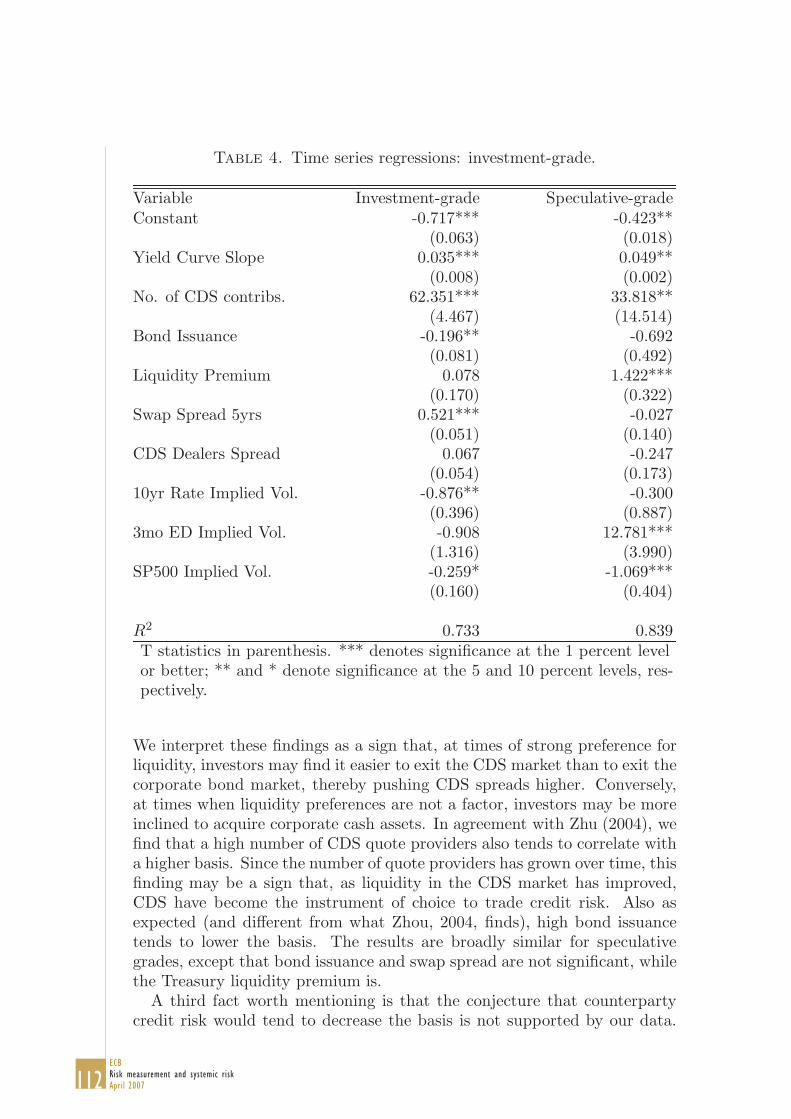
112ECBRisk measurement and systemic riskApril 2007
Table 4. Time series regressions: investment-grade.
Variable Investment-grade Speculative-gradeConstant -0.717*** -0.423**
(0.063) (0.018)Yield Curve Slope 0.035*** 0.049**
(0.008) (0.002)No. of CDS contribs. 62.351*** 33.818**
(4.467) (14.514)Bond Issuance -0.196** -0.692
(0.081) (0.492)Liquidity Premium 0.078 1.422***
(0.170) (0.322)Swap Spread 5yrs 0.521*** -0.027
(0.051) (0.140)CDS Dealers Spread 0.067 -0.247
(0.054) (0.173)10yr Rate Implied Vol. -0.876** -0.300
(0.396) (0.887)3mo ED Implied Vol. -0.908 12.781***
(1.316) (3.990)SP500 Implied Vol. -0.259* -1.069***
(0.160) (0.404)
R2 0.733 0.839T statistics in parenthesis. *** denotes significance at the 1 percent levelor better; ** and * denote significance at the 5 and 10 percent levels, res-pectively.
We interpret these findings as a sign that, at times of strong preference forliquidity, investors may find it easier to exit the CDS market than to exit thecorporate bond market, thereby pushing CDS spreads higher. Conversely,at times when liquidity preferences are not a factor, investors may be moreinclined to acquire corporate cash assets. In agreement with Zhu (2004), wefind that a high number of CDS quote providers also tends to correlate witha higher basis. Since the number of quote providers has grown over time, thisfinding may be a sign that, as liquidity in the CDS market has improved,CDS have become the instrument of choice to trade credit risk. Also asexpected (and different from what Zhou, 2004, finds), high bond issuancetends to lower the basis. The results are broadly similar for speculativegrades, except that bond issuance and swap spread are not significant, whilethe Treasury liquidity premium is.
A third fact worth mentioning is that the conjecture that counterpartycredit risk would tend to decrease the basis is not supported by our data.

113ECB
Risk measurement and systemic riskApril 2007
Table 5. The persistence of the aggregate bases.
Unconditional Conditionalρ h ρ|X h|X
Investment-grade 0.909 7.250 0.577 1.259Speculative-grade 0.845 4.108 0.691 1.872
The coefficient on the CDS spread of large dealers is statistically insignifi-cant for both investment-grade and speculative-grade credits, and has thewrong sign (positive) for the former. It could be that, precisely because thevast majority of CDS trades have a large dealer as a counterpart, counter-party credit risk is not of great concern to investors. In other words, thecredit quality of those dealers has remained excellent throughout our sampleperiod, and its variation may not have been enough to produce a noticeableeffect on the basis.
Uncertainty about macroeconomic conditions—as proxied by the S&P500 implied volatility—has a negative effect on the basis. The volatility ofthe ten-year Treasury yield has a similar effect, but is significant only inthe investment-grade case. These negative signs indicate that, at times ofheightened macroeconomic uncertainty, the bond market tends to sell off ata faster pace than the CDS market. Interestingly, uncertainty about themonetary policy path, as proxied by the implied volatility on the three-month eurodollar rate, has a positive and highly significant effect on thespeculative-grade basis.
Finally, we note that the R2 are fairly high for both sets of firms, and es-pecially so for investment-grade firms, indicating that our set of explanatoryvariables captured most of the aggregate variation in the basis.
The persistence of deviations of the aggregate bases away from theirmeans is also interesting, since it gives a sense of how fast the aggregatebases tend to return to zero, and thus how fast market frictions induced bysystematic effects tend to disappear. One way to study persistence is to sim-ply look at the estimated autoregressive coefficient of the investment-gradeand speculative-grade bases; another would be to examine the estimatedautoregressive coefficient conditional on the explanatory variables containedin the matrix X. Table 5 contains those estimates. We find it useful totransform the correlation coefficients into half lives, which are measures ofthe time it takes a process with a certain autocorrelation coefficient to re-turn half way to its mean upon displacement. In particular, we define theunconditional half life h as:
(4) h =log(0.5)log(ρ)
and the conditional half life analogously. Unconditionally, the estimated au-tocorrelation coefficients are fairly high. As a consequence, it takes more

114ECBRisk measurement and systemic riskApril 2007
than 7 weeks for the investment-grade basis to return to its mean; thespeculative-grade basis takes instead more than four weeks. Conditionallyon our explanatory variables, however, the half lives are much shorter, withboth of them under two weeks.21 We view this as a further confirmation thatwe capture the most relevant aggregate factors that induce wedges betweenthe CDS and cash market.
5. The bond-specific component of the Basis
As we discussed in section 3, credit default swap spreads tend to be sys-tematically higher or lower than bond spreads for long periods of time fora number of bonds. In this section, we study possible factors that mayconcur to determine the average level of the basis across bonds and firms.Our dataset contains several variables that are either bond-specific or firm-specific that could potentially be informative as to why idiosyncratic typesof frictions may prevail between the two markets. Bond-specific variablesinclude maturity, credit rating, the size of the issuance, and price; firm-specific variables include the recovery rate as estimated by the contributorsto the Markit dataset, the number of contributors that provide CDS quotesat the five-year maturity, the firm’s equity implied volatility, and the sectorin which the firm operates.
All of the variables mentioned above, which include measures of liquidityand distress, as well as purely technical factors, could potentially play a rolein determining whether it could be possible or cost-effective to arbitrageaway any differences between CDS and bond spreads. For example, theavailability of corporate bonds in the repo market, and therefore the pos-sibility of shorting them, may depend on the size of the outstanding bondissue. Poor liquidity in the CDS market may result in high transaction coststhat may compromise investors’ ability to take advantage of arbitrage oppor-tunities. High firm-specific implied volatilities may be a sign that firms areexperiencing difficulties that may create imbalances in the relative demandand supply for their securities. Finally, there may be bond-specific factorsthat, while not immediately obvious, may still play a role in determiningthe presence and the extent of market frictions.
Our list of firm- or bond-specific variables could be useful in explaining notjust the behavior of the average basis across time, but also of several otherproperties of the basis. For example, we believe that understanding someof the factors that may help account for the dispersion of the basis acrossfirms is equally important from the perspective of understanding frictions inthe corporate market. And so is understanding the factors that may affectthe persistence of deviations of each bond’s basis around its mean, as well
21Note that, when adding a lagged basis term to equation 3, the signs and the signifi-cance of the coefficients reported in table 4 do not change.
115ECB
Risk measurement and systemic riskApril 2007
as around the aggregate basis βt. Our strategy is to run a series of cross-sectional regressions using the explanatory variables mentioned above. Ourregressions are of the type:
αk = a1Zk + εk
σk = a2Zk + εk
hk = a3Zk + εk
φk = a4Zk + εk
where αk denotes the bond-specific effects estimated in section 3, σk de-notes their volatility over time, hk is the estimated half-life of the basisdeviations, and φ represents the “beta” of each individual basis.
Specifically,
(5) hk =log(0.5)log(ρk)
,
where ρk is the estimate of the first-order autoregressive coefficient of eachindividual basis obtained from bkt = µk + ρkbkt−1 + ekt. Similarly, φk, ourmeasure of the basis “beta,” is obtained from a series of regressions of thetype:
(6) bkt = µk + φkβt + ekt
Our explanatory variables are grouped in the matrix Zk as time averages ofthe variables listed at the beginning of the section,
The results are reported in tables 6 (for the average and standard devi-ation of the basis), and 7 (for the half-life and the “beta.” From the R2 itis clear that our variables are more effective at explaining the variation inαk than its level, while they do not do a particularly good job at explainingeither the half-life or the “beta.”
For the typical firm, it seems that bond size has a positive effect onthe basis, everything else equal; in other words, large bonds tend to havea higher basis than smaller bonds in our dataset. While this may seemcounterintuitive, we speculate that it may reflect the difficulty of shortingbonds with a large amount outstanding, perhaps because those bonds areheld by large investors who have no interest in making them available in therepo market. Consistent with this interpretation, the basis for large bondsis less dispersed around its mean. The fact that, on average, bonds of longmaturity also seem to have a larger basis may also be consistent with ourprevious interpretation, as long bonds tend to be larger in size and may beheld by “steady money” investors.
An alternative interpretation could be that holders of the largest bondstend to resort more to the CDS market to buy protection, and are willing topay for it. This interpretation may be partially supported by the fact thatbond size and maturity also tend to significantly reduce the time the basistakes to return to its mean once it is displaced. It could be that, once the

116ECBRisk measurement and systemic riskApril 2007
Table 6. Cross-sectional regressions: basis mean and stan-dard deviation.
Variable αk σk
Average Maturity 5.872*** -0.005(1.225) (0.517)
(Average Maturity)2 -0.343*** -0.067(0.108) (0.045)
Bond size (log) 7.905*** -1.583***(1.074) (0.385)
Coupon -3.083*** 1.886***(0.443) (0.198)
Implied Vol. (avg.) 0.285*** 0.167***(0.092) (0.033)
Implied Vol. (std.) -0.173 0.186(0.215) (0.128)
Recovery (avg.) -1.291*** 0.126**(0.181) (0.063)
Credit Spread Vol. -0.006 0.051***(0.014) (0.014)
High Yield 9.800*** 5.877***(2.041) (0.923)
No. of Downgrades 3.183*** 1.228*(1.109) (0.634)
No. of Upgrades 0.777 -0.556(1.322) (0.648)
No. of CDS contributors (avg.) -0.596*** -0.043(0.184) (0.056)
Sector Dummies *** ***F=5.571 F=3.63
R2 0.344 0.646T statistics in parenthesis. *** denotes significance at the 1 percent levelor better; ** and * denote significance at the 5 and 10 percent levels, res-pectively.
reasons for concern disappear, investors in those bonds are quick to shedprotection in the CDS market, thereby returning the basis to its normallevel.
Bonds that have been downgraded often also tend to have a higher andmore dispersed basis on average, and so do bonds that belong (or have

117ECB
Risk measurement and systemic riskApril 2007
Table 7. Cross-sectional regressions: basis half-life and “beta.”
Variable hk φk
Average Maturity 0.487 0.155*(0.407) (0.083)
(Average Maturity)2 -0.072** -0.009(0.034) (0.007)
Bond size (log) -1.628*** -0.012(0.318) (0.074)
Coupon 0.918*** 0.098***(0.128) (0.032)
Implied Vol. (avg.) -0.089*** 0.002(0.019) (0.006)
Implied Vol. (std.) 0.185*** -0.034**(0.058) (0.017)
Recovery (avg.) 0.118*** 0.015(0.038) (0.010)
Credit Spread Vol. -0.007* 0.001(0.004) (0.001)
High Yield -1.321** -0.196(0.622) (0.128)
No. of Downgrades 1.122** 0.105(0.563) (0.109)
No. of Upgrades 0.760 -0.121(0.999) (0.083)
No. of CDS contributors (avg.) 0.127** -0.005(0.056) (0.010)
Sector Dummies *** ***F=4.833 F=3.63
R2 0.105 0.039T statistics in parenthesis. *** denotes significance at the 1 percent levelor better; ** and * denote significance at the 5 and 10 percent levels, res-pectively.
belonged for at least one day) to the high-yield universe.22 In agreementwith common intuition, bonds that have been downgraded the most alsotend to have longer half lives; high-yield bonds that have not been subjectto many rating changes, however, have shorter half lives, everything elseequal.
22Our high-yield indicator takes on the value of one if a bond has ever been ratedbelow BBB, and zero otherwise. We do not separate bonds into investment-grade andspeculative-grade categories because those categories are not the same over time.

118ECBRisk measurement and systemic riskApril 2007
Bonds whose issuer has a high average implied volatility over our sampletend to have higher and more volatile bases. This could again reflect thefact that investors find it easy to seek and obtain protection in the CDSmarket for firms that are riskier than other or that are perceived as beingin distress for prolonged periods of time. The deviations of the basis awayfrom the mean for those high-volatility firms, however, tend to be shorter,perhaps because the bond market does not take much longer to react.23 Insomewhat of a puzzle, the volatility of implied volatility does not seem tohave an effect on either the level or the standard deviation of the averagebasis. We interpret the volatility of implied volatility as an indicator thata firm has undergone periods of stress while its bonds were in our sample,and thus we would expect its basis to be, on average, higher than normal ifit is true that investors prefer the CDS market at times of stress.24 We alsonote that a high volatility of volatility significantly lengthens the half lifeof the basis, and reduces φk (indeed, it is one of the few factors that enterssignificantly in the basis “beta” in equation 6).
High CDS liquidity, as proxied by the number of dealers willing to provideCDS quotes in the Markit dataset, tends to lower the basis, on average.Admittedly, this is not a perfect measure of liquidity, as at any given timethere may be many dealers willing to provide quotes with extremely highbid-ask spreads, or many of those dealers may be providing very expensivequotes to protection seekers. Still, we find our result interesting, because itmay point to poor liquidity conditions in the CDS market as a cause for high,positive bases. Also, the negative sign of the liquidity coefficient in the cross-sectional regressions is in contrast with the positive sign the correspondingcoefficient has in the time series regressions. We are investigating this pointfurther and we will report more results in future versions of the paper.
Finally, we note that high recovery rates tend to reduce the basis, asdo bonds with large coupons. Intuitively, while the coupon effect may betechnical in nature, the higher the recovery rate, the lower the credit riskthat investors face, and thus the less incentives investors will have to seekpricey protection in the CDS market. The sector that a firm belongs to alsoappears to be significant in determining the level, dispersion, persistence,and “beta” of the average bond-specific basis. This may be because firmsin certain sectors are more likely to experience common shocks.
6. Conclusions
We proposed to quantify the degree of corporate market functioning bythe extent to which seeming arbitrage opportunities remain persistently un-exploited. We defined those arbitrage opportunities in term of the basis,
23Both Blanco et al. (2005) and Zhu (1994) find that the CDS market leads the cashmarket in the price discovery process.
24Our interpretation is consistent with the GM experience plotted in figure 4: GM’sbasis surges in the spring of 2005 when the firm’s credit quality deteriorated fast and itsimplied volatility spiked.

119ECB
Risk measurement and systemic riskApril 2007
the difference between the CDS and corporate bond spread. We find thata large fraction of the variation in the basis across a large sample of bondsand firms is idiosyncratic in nature and reflects factors that are specific toa particular bond or firm.
Aggregate macroeconomic and financial variables account for a smaller,though certainly not negligible, fraction of the total variation in the basis.A large portion of the aggregate variation can be explained by variablesrelated to liquidity conditions and liquidity preferences, as well as to theshape of the yield curve and the uncertainty about future economic andfinancial conditions.
In future research we plan to expand our analysis to the study of mar-ket frictions in a panel setting, where bond- and firm-specific variables areallowed to have a different effect on the basis over time. In a related, event-study type of project we are also working to understand the effects of ag-gregate and idyiosincratic shocks on the basis. We plan to proxy aggregateshocks with macroeconomic and monetary policy surprises, while we definefirm-specific shocks in terms of the discrepancy between actual and expectedearnings releases. We believe that those shocks may be yet another sourceof frictions in the corporate market, and some preliminary results supportthat belief.
References
Acharya, V.V., and Johnson, T.C. (2005): Insider Trading in Credit Deriva-tives. CEPR Discussion Paper no. 5180.
Alexander, G.J., Edwards, A.K., and Ferri, M.G. (2000): The determinantsof trading volume of high-yield corporate bonds. Journal of Finan-
cial Markets, vol.3, May, pp. 177–204.Apedjinou, K.M. (2003): What drives interest rate swap spreads? Mimeo,
Columbia University.Bank for International Settlements (2005): Triennial central bank survey:
foreign exchange and derivatives market activity in 2004. Availableat www.bis.org.
Beinstein, E. (2005): Using credit derivatives to implement your creditviews. J.P. Morgan, presentation at the 2005 Credit Derivativesand Structured Credit Conference.
Blanco, R., Brennan, S., and Marsh, I. (2005): An empirical analysis ofthe dynamic relationship between investment-grade bonds and creditdefault swaps. The Journal of Finance, forthcoming.
Bomfim, A.N. (2005): Understanding Credit Derivatives and Related In-
struments. London, Elsevier Academic Press.Calamaro, J.P., and Tierney, J.F. (2004): Trading the CDS-bond basis. In
Deutsche Bank’s Quantitative Credit Strategy, March 26.Duffie, D. (1999): Credit Swap Valuation. Financial Analysts Journal, vol.
55, pp. 73-87.

120ECBRisk measurement and systemic riskApril 2007
Duffie, D. and Liu, J. (1999): Floating-Fixed Credit Spreads. Workingpaper, Stanford University.
Duffie, D., Singleton, K.J. (2003): Credit Risk: Pricing, Measurement, and
Management. Princeton, Princeton University Press.Gibson, M. (2004): Understanding the risk of synthetic CDOs. Federal
Reserve Board, FEDS Working Papers Series no. 2004-36.Greenblatt, M. (2002): An analytic solution for interest rate swap spreads.
Yale ICF Working Paper no. 2002-02.Houweling, P., Mentink, A., and Vorst, T. (2005): Comparing possible prox-
ies of corporate bond liquidity. Journal of Banking and Finance, vol.29, no. 6, pp. 1331–1358.
Houweling, P., and Vorst, T. (2005): Pricing default swaps: empirical evi-dence. Journal of International Money and Finance, forthcoming.
Hull, J., Pedrescu, M., and White, A. (2003): The relationship betweencredit default swap spreads, bond yields, and credit rating announce-ments. Working paper, University of Toronto.
Longstaff, F., Mithal, S., and Neis, E. (2004): The credit default swapmarket: is credit protection priced correctly? NBER Working PaperSeries no. 10418.
Meng, L. and Gwilym O.A. (2005): Credit default swaps: theory and em-pirical evidence. The Journal fo Fixed Income, March.
Norden, L. and Weber, M. (2004): Informational efficiency of credit defaultswap and stock markets: the impact of credit rating announcements.CEPR Discussion Paper series, no. 4250.
O’Kane, D., and McAdie, R (2001): Explaining the basis: cash versusdefault swaps. Lehman Brohters, Structure Credit Research, May.
Schultz, P. (2001): Corporate bond trading costs: a peak behind the curtain.The Journal of Finance, vol. 61, no.2, pp. 677–698.
Zhang, Y., Zhou, H., and Zhu, H. (2005): Explaining credit default swapsprads with equity volatility and jump risks of individual firms. Man-uscript.
Zhu, H. (2004): An empirical comparison of credit spreads between the bondmarket and the credit default swap market. BIS Working Paper no.160.

121ECB
Risk measurement and systemic riskApril 2007
SESSION 4
SYSTEMIC RISK
ACROSS COUNTRIES
122ECBRisk measurement and systemic riskApril 2007
BANKING SYSTEM STABILITYA CROSS-ATLANTIC PERSPECTIVE1
BY PHILIPP HARTMANN2, STEFAN STRAETMANS3 AND CASPER DE VRIES4
1 Paper prepared for the NBER project on “Risks of Financial Institutions”.We benefited from suggestions and criticism by many participants in the project, in particular by the organizers Mark Carey (also involving Dean Amel and Allen Berger) and Rene Stulz, by our discussant Tony Saunders and by Patrick de Fontnouvelle, Gary Gorton, Andy Lo, Jim O’Brien and Eric Rosengren. Furthermore, we are grateful for comments we received at the 2004 European Finance Association Meetings in Maastricht, in particular by our discussant Marco da Rin and by Christian Upper, at the 2004 Ottobeuren seminar in economics, notably the thoughts of our discussant Ernst Baltensberger, of Friedrich Heinemann and of Gerhard Illing, as well as at seminars of the Max Planck Institute for Research on Collective Goods, the Federal Reserve Bank of St. Louis, the ECB and the University of Frankfurt. Gabe de Bondt and David Marques Ibanez supported us enormously in finding yield spread data, Lieven Baele and Richard Stehle kindly made us aware of pitfalls in Datastream equity data.Very helpful research assistance by Sandrine Corvoisier, Peter Galos and Marco Lo Duca as well as editorial support by Sabine Wiedemann are gratefully acknowledged. Any views expressed only reflect those of the authors and should not be interpreted as the ones of the ECB or the Eurosystem.2 CEPR and European Central Bank, DG Research, Kaiserstrasse 29, 60311 Frankfurt am Main, Germany; e-mail: [email protected], URL: http://papers.ssrn.com/sol3/cf_dev/AbsByAuth.cfm?per_id=2294143 Limburg Institute of Financial Economics (LIFE), Economics Faculty, Maastricht University, P.O. Box 616, 6200 MD Maastricht, The Netherlands; e-mail address: [email protected], URL: http://www.fdewb.unimaas.nl/finance/faculty/straetmans/4 Faculty of Economics, Erasmus University Rotterdam, P.O. Box 1738, 3000 DR Rotterdam,The Netherlands; e-mail: [email protected], URL: http://www.few.eur.nl/people/cdevries/

123ECB
Risk measurement and systemic riskApril 2007
Abstract
This paper derives indicators of the severity and structure of banking system risk from asymptotic interdependencies between banks’ equity prices. We use new tools available from multivariate extreme value theory to estimate individual banks’ exposure to each other (“contagion risk”) and to systematic risk. By applying structural break tests to those measures we study whether capital markets indicate changes in the importance of systemic risk over time. Using data for the United States and the euro area, we can also compare banking system stability between the two largest economies in the world. For Europe we assess the relative importance of cross-border bank spillovers as compared to domestic bank spillovers. The results suggest, inter alia, that systemic risk in the US is higher than in the euro area, mainly as cross-border risks are still relatively mild in Europe. On both sides of the Atlantic systemic risk has increased during the 1990s.
Key words and phrases: Banking, Systemic Risk, Asymptotic Dependence, Multivariate Extreme Value Theory, Structural Change Tests
JEL classification: G21, G28, G29, G12, C49
Reprinted from M. Carey and R. Stulz (eds., 2006), Risks of Financial Institutions (Chicago University Press and National Bureau of Economic Research), pages 133 - 188, with kind permission of the Chicago University Press and the NBER.

124ECBRisk measurement and systemic riskApril 2007
Non-technical summary
A particularly important sector for the stability of financial systems is the banking sector. Banking sectors in major economies such as the United States and the euro area have been subject to considerable structural changes. For example, the US (and Europe) have experienced substantial banking consolidation since the 1990s and the emergence of large and complex institutions. The establishment of the conditions for the single market for financial services in the EU in conjunction with the EMU has led to progressing banking integration. These structural changes have made the monitoring of banking system stability even more complex. In Europe, for example, issues are raised about how to pursue macroprudential surveillance in a context of national banking supervision.
For all these reasons the present paper presents a new approach how to assess banking system risk, whether it is domestic or cross-border. This approach is based on new techniques available from multivariate extreme value theory, a statistical approach to assess the joint occurrence of very rare events, such as severe banking problems. More precisely, as measures of systemic risk we estimate semi-parametrically the probability of crashes in bank stocks, conditional on crashes of other bank stocks or of the market factor. The data cover the 50 most important banks in the US and in the euro area between 1992 and 2004. We estimate the amount of systemic risk in the euro area and in the US, and compare it across the Atlantic. We also compare domestic risk to cross-border risk and, finally, we test for structural change in systemic risk over time.
Our results suggest that the risk of multivariate extreme spillovers between US banks is higher than between European banks. Hence, despite the fact that available balance-sheet data show higher interbank exposures in the euro area, the US banking system seems to be more prone to contagion risk. Second, the lower spillover risk among European banks is mainly related to relatively weak cross-border linkages. Domestic linkages in France, Germany and Italy, for example, are of the same order as domestic US linkages. One interpretation of this result is that further banking integration in Europe could lead to higher cross-border contagion risk in the future, with the more integrated US banking system providing a benchmark. Third, cross-border spillover probabilities tend to be smaller than domestic spillover probabilities, but only for a few countries this difference is statistically significant. For example, among the banks from a number of larger countries – such as France, Germany, the Netherlands and Spain – extreme cross-border linkages are statistically indistinguishable from domestic linkages. In contrast, the effects of banks from these larger countries on the main banks from some smaller countries – including particularly Finland and Greece,

125ECB
Risk measurement and systemic riskApril 2007
and sometimes also Ireland or Portugal – tend to be significantly weaker than the effects on their domestic banks. Hence, those smaller countries located further away from the center of Europe seem to be more insulated from European cross-border contagion.
Fourth, the effects of macro shocks on banking systems are similar in the euro area and the US, and they illustrate the relevance of aggregate risks for banking system stability. While stock market indices perform well as indicators of aggregate risk, we find that high-yield bond spreads capture extreme systematic risk for banks relatively poorly, both in Europe and the US. Fifth, structural stability tests for our indicators suggest that systemic risk, both in the form of interbank spillovers and in the form of aggregate risk, has increased in Europe and in the US. Our tests detect the break points during the second half of the 1990s, but graphical illustrations of our extreme dependence measures show that this was the result of developments spread out over time. In particular in Europe the process was very gradual, in line with what one would expect during a slowly advancing financial integration process. Interestingly, the introduction of the euro in January 1999 seems to have had a reductionary or no effect on banking system risk in the euro area. This may be explained by the possibility that stronger cross-border crisis transmission channels through a common money market could be offset by better risk sharing and the better ability of a deeper market to absorb shocks.

126ECBRisk measurement and systemic riskApril 2007
1. Introduction
A particularly important sector for the stability of nancial systems
is the banking sector. Banks play a central role in the money cre-
ation process and in the payment system. Moreover, bank credit is an
important factor in the nancing of investment and growth. Faltering
banking systems have been associated with hyperin ations and depres-
sions in economic history. Hence, to preserve monetary and nancial
stability central banks and supervisory authorities have a special inter-
est in assessing banking system stability.
This is a particularly complex task in very large economies with
highly developed nancial systems, such as the United States and the
euro area. Moreover, structural changes in the nancial systems of
both these economies make it particularly important to track risks
over time. In Europe, gradually integrating nancial systems under
a common currency increase the relationships between banks across
borders. This development raises the question how banking systems
should be monitored in a context where banking supervision in con-
trast to monetary policy remains a national responsibility. In the
US, tremendous consolidation as well as the removal of regulatory bar-
riers to universal and cross-state banking has led to the emergence of
large and complex banking organizations (LCBOs), whose activities
and interconnections are particularly di cult to follow. For all these
reasons we present a new approach how to assess banking system risk
in this paper and apply it to the euro area and the US.
A complication in assessing banking system stability is that, in con-
trast to other elements of the nancial system, such as securities values,
interbank relationships that can be at the origin of bank contagion phe-
nomena or the values of and correlations between loan portfolios are
particularly hard to measure and monitor.1 Hence, a large part of
the published banking stability literature has resorted to more indi-
rect market indicators. In particular, spillovers in bank equity prices
have been used for this purpose.2 Pioneered by Aharony and Swary
(1983) and Swary (1986) a series of papers have applied the event
1Even central banks and supervisory authorities usually do not have continuous
information about interbank exposures. For the Swedish example of a central bank
monitoring interbank exposures at a quarterly frequency, see Blavarg and Nimander
(2002).2The choice of bank equity prices for measuring banking system risk may be mo-
tivated by Merton’s (1974) option-theoretic framework toward default. The latter
approach has become the cornerstone of a large body of approaches for quanti-
fying credit risk and modeling credit rating migrations, including J.P. Morgan’s
CreditMetrics (1999).

127ECB
Risk measurement and systemic riskApril 2007
study methodology to the e ects of speci c bank failures or bad news
for certain banks on other banks’ stock prices (see, e.g., also Wall and
Petersen, 1990; Docking, Hirschey and Jones, 1997; Slovin, Sushka
and Polonchek, 1999). In another series of papers various regression
approaches are used in order to link abnormal bank stock returns to
asset-side risks, including those related to aggregate shocks (see, e.g.,
Cornell and Shaphiro, 1986; Smirlock and Kaufold, 1987; Musumeci
and Sinkey, 1990; or Kho, Lee and Stulz, 2000). De Nicolo and Kwast
(2002) relate changes in correlations between bank stock prices over
time to banking consolidation. Gropp and Moerman (2004) measure
conditional co-movements of large abnormal bank stock returns and of
equity-derived distances to default. Gropp and Vesala (2004) apply an
ordered logit approach to estimate the e ect of shocks in distances to
default for some banks on other banks’ distances to default.3
Some authors point out that most banking crises have been related to
macroeconomic uctuations rather than to prevalent contagion. Gor-
ton (1988) provides ample historical evidence for the US, Gonzalez-
Hermosillo, Pazarbasioglu and Billings (1997) also nd related evidence
3Other market indicators used in the literature to assess bank contagion include
bank debt risk premia (see, in particular, Saunders (1986) and Cooperman, Lee
and Wolfe (1992)).
A number of approaches that do not rely on market indicators have also been
developed in the literature. Grossman (1993) and Hasan and Dwyer (1994) measure
autocorrelation of bank failures after controlling for macroeconomic fundamentals
during various episodes of US banking history. Saunders and Wilson (1996) study
deposit withdrawals of failing and non-failing banks during the Great Depression.
Calomiris and Mason (1997) look at deposit withdrawals during the 1932 banking
panic and ask whether also ex ante healthy banks failed as a consequence of them.
Calomiris and Mason (2000) estimate the survival time of banks during the Great
Depression, with explanatory variables including national and regional macro fun-
damentals, dummies for well known panics and the level of deposits in the same
county (contagion e ect).
A recent central banking literature attempts to assess the importance of conta-
gion risk by simulating chains of failures from (incomplete and mostly con dential)
national information about interbank exposures. See, e.g., Fur ne (2003), Elsinger,
Lehar and Summer (2002), Upper and Worms (2004), Degryse and Nguyen (2004),
Lelyveld and Liedorp (2004) or Mistrulli (2005).
Chen (1999), Allen and Gale (2000) and Freixas, Parigi and Rochet (2002) de-
velop the theoretical foundations of bank contagion.

128ECBRisk measurement and systemic riskApril 2007
for the Mexican crisis of 1994-1995 and Demirgüc-Kunt and Detra-
giache (1998) add substantial further support for this hypothesis using
a large multi-country panel dataset.4
The new approach for assessing banking system risk presented in
this paper also employs equity prices. It is based on extreme value
theory (EVT) and allows us to estimate the probabilities of spillovers
between banks, their vulnerability to aggregate shocks and changes in
those risks over time. More precisely, we want to make three main con-
tributions compared to the previous literature. First, we use the novel
multivariate extreme value techniques applied by Hartmann, Straet-
mans and de Vries (2003a/b and 2004) and Poon, Rockinger and Tawn
(2004) to estimate the strength of banking system risks. In particu-
lar, we distinguish conditional “co-crash” probabilities between banks
from crash probabilities conditional on aggregate shocks. While EVT
- both univariate and multivariate - has been applied to general stock
indices before, it has not yet been used to assess the extreme depen-
dence between bank stock returns with the aim to measure banking
system risk. Second, we cover both euro area countries and the United
States to compare banking system stability internationally. We are not
aware of any other study that tries to compare systemic risk between
these major economies. Third, we apply the test of structural stability
for tail indexes by Quintos, Fan and Phillips (2001) to the multivariate
case of extreme linkages and assess changes in banking system stability
over time with it. Again, whereas a few earlier papers addressed the
changing correlations between bank stock returns, none focused on the
extreme interdependence we are interested in in the present paper.
The idea behind our approach is as follows. We assume that bank
stocks are e ciently priced, in that they re ect all publicly available
information about (i) individual banks’ asset and liability side risks
and (ii) relationships between di erent banks’ risks (be it through cor-
relations of their loan portfolios, interbank lending or other channels).
We identify a critical situation of a bank with a dramatic slump of its
stock price. We identify the risk of a problem in one or several banks
spilling over to other banks (“contagion risk”) with extreme negative
co-movements between individual bank stocks (similar to the condi-
tional co-crash probability in our earlier stock, bond and currency pa-
pers). In addition, we identify the risk of banking system destabiliza-
tion through aggregate shocks with the help of the “tail- ” proposed
4Hellwig (1994) argues that the observed vulnerability of banks to macroeco-
nomic shocks may be explained by the fact that deposit contracts are not condi-
tional on aggregate risk. Chen (1999) models, inter alia, how macro shocks and
contagion can reinforce each other in the banking system.
129ECB
Risk measurement and systemic riskApril 2007
by Straetmans, Verschoor and Wolf (2003). The tail- is measured
by conditioning our co-crash probability on a general stock index (or
another measure of systematic risk) rather than on individual banks’
stock prices. Therefore, in some respects it re ects the tail equivalent
to standard asset pricing models. In this paper we further extend the
analysis of tail- by also using high-yield bond spreads as measures of
aggregate risk. Based on the estimated individual co-crash probabil-
ities and tail- s, we can then test for the equality of banking system
risk between the US and the euro area and for changes in systemic risk
over time.
Our work is also related to an active literature examining which phe-
nomena constitute nancial contagion and how they can be identi ed
empirically. In our reading, the main criteria proposed so far to identify
contagion are that (i) a problem at a nancial institution adversely af-
fects other nancial institutions or that a decline in an asset price leads
to declines in other asset prices; (ii) the relationships between failures
or asset price declines must be di erent from those observed in normal
times (regular “interdependence”); (iii) the relationships are in excess
of what can be explained by economic fundamentals; (iv) the events
constituting contagion are negative “extremes”, such as full-blown in-
stitution failures or market crashes, so that they correspond to crisis
situations; (v) the relationships are the result of propagations over time
rather than being caused by the simultaneous e ects of common shocks.
Most empirical approaches proposed in the recent literature how to
measure contagion capture the rst criterion (i), but this is where the
agreement usually ends. Authors di er in their view which of the other
criteria (ii) through (v) are essential for contagion. Forbes and Rigobon
(2002) stress statistically signi cant changes in correlations over time
as a contagion indicator and illustrate how they emerge among emerg-
ing country equity markets. Shiller (1989), Pindyck and Rotemberg
(1993) and Bekaert, Harvey and Ng (forthcoming) emphasize “excess
co-movements” between stock markets and stock prices, beyond what
is explained in various forms of regressions by dividends, macroeco-
nomic fundamentals or asset pricing “factors”. Eichengreen, Rose and
Wyplosz (1996) estimate probit models to examine whether the occur-
rence of a balance-of-payments crisis in one country increases the prob-
ability of a balance-of-payments crisis in other countries, conditional on
macroeconomic country fundamentals. Bae, Karolyi and Stulz (2003)
propose the logit regression model to estimate probabilities that several
stock markets experience large negative returns, given that a smaller
number of stock markets experience large negative returns, conditional
on interest and exchange rates. Longin and Solnik (2001) are among

130ECBRisk measurement and systemic riskApril 2007
the rst to apply bivariate EVT to estimate extreme equity market
correlations, also assuming the logistic distribution. Hartmann et al.
(2003a/b, 2004) stress that market co-movements far out in the tails
(“asymptotic dependence”) may be very di erent from regular depen-
dence in multivariate distributions and that such crisis behavior may
not have the same parametric form in di erent markets. Based on a
di erent branch of EVT, they estimate semi-parametrically for stocks,
bonds and currencies the likelihood of widespread market crashes con-
ditional on contemporaneous and lagged other market crashes. The
reason why we particularly focus on criterion (iv) is that it allows us to
concentrate on events that are severe enough to be basically always of
a concern for policy. Other criteria are also interesting and have their
own justi cations, but more regular propagations or changes in them
are not necessarily a concern for policies that aim at the stability of
nancial systems.5
The data we use in this work are daily bank stock excess returns
in euro area countries and the United States between April 1992 and
February 2004. For each area or country we choose 25 banks based on
the criteria of balance-sheet size and involvement in interbank lending.
So, our sample represents the systemically most relevant nancial in-
stitutions, but neglects a large number of smaller banks. During our
sample period several of the banks selected faced failure-like situations
and also global markets passed several episodes of stress. All in all, we
have about 3,100 observations per bank.
Our results suggest that the risk of multivariate extreme spillovers
between US banks is higher than between European banks. Hence, de-
spite the fact that available balance-sheet data show higher interbank
exposures in the euro area, the US banking system seems to be more
prone to contagion risk. Second, the lower spillover risk among Euro-
pean banks is mainly related to relatively weak cross-border linkages.
Domestic linkages in France, Germany and Italy, for example, are of
the same order as domestic US linkages. One interpretation of this re-
sult is that further banking integration in Europe could lead to higher
cross-border contagion risk in the future, with the more integrated US
banking system providing a benchmark. Third, cross-border spillover
probabilities tend to be smaller than domestic spillover probabilities,
but only for a few countries this di erence is statistically signi cant.
5Less extreme spillovers might still indicate some form of microeconomic ine -
ciencies but not necessarily widespread destabilization.
De Bandt and Hartmann (2000) provide a more complete survey of the market
and banking contagion literature. Pritsker (2001) discusses di erent channels of
contagion.

131ECB
Risk measurement and systemic riskApril 2007
For example, among the banks from a number of larger countries
such as France, Germany, the Netherlands and Spain extreme cross-
border linkages are statistically indistinguishable from domestic link-
ages. In contrast, the e ects of banks from these larger countries on
the main banks from some smaller countries including particularly
Finland and Greece, and sometimes also Ireland or Portugal tend to
be signi cantly weaker than the e ects on their domestic banks. Hence,
those smaller countries located further away from the center of Europe
seem to be more insulated from European cross-border contagion.
Fourth, the e ects of macro shocks emphasized by the estimated
tail- s are similar for the euro area and the US, and they illustrate
the relevance of aggregate risks for banking system stability. While
stock market indices perform well as indicators of aggregate risk, we
nd that high-yield bond spreads capture extreme systematic risk for
banks relatively poorly, both in Europe and the US. Fifth, structural
stability tests for our indicators suggest that systemic risk, both in the
form of interbank spillovers and in the form of aggregate risk, has in-
creased in Europe and in the US. Our tests detect the break points
during the second half of the 1990s, but graphical illustrations of our
extreme dependence measures show that this was the result of devel-
opments spread out over time. In particular in Europe the process was
very gradual, in line with what one would expect during a slowly ad-
vancing nancial integration process. Interestingly, the introduction of
the euro in January 1999 seems to have had a reductionary or no e ect
on banking system risk in the euro area. This may be explained by
the possibility that stronger cross-border crisis transmission channels
through a common money market could be o set by better risk sharing
and the better ability of a deeper market to absorb shocks.
The paper is structured as follows. The next section describes our
theoretical indicators of banking system stability, distinguishing the
multivariate spillover or contagion measure from the aggregate tail-
measure for stock returns. Section 3 outlines the estimation procedures
for both measures; and section 4 presents two tests, one looking at the
stability of spillover and systematic risk over time and the other looking
at the stability of both measures across countries and continents (cross-
sectional stability). Section 5 summarizes the data set we employ, in
particular how we selected the banks covered, provides some standard
statistics for the individual bank and index returns, and gives some
information about the occurrence of negative extremes for individual
banks and the related events.

132ECBRisk measurement and systemic riskApril 2007
Section 6 then presents the empirical results on extreme bank spillover
risks. For both the euro area and the US we estimate the overall multi-
variate extreme dependence in the banking sector and we test whether
one is larger than the other. Moreover, for Europe we assess whether
domestic spillover risk is stronger or weaker than cross-border risk. Sec-
tion 7 turns to the empirical results for aggregate banking system risk
on both continents. We estimate individual tail- s for European banks
and for US banks. We also aggregate those s and test for the equality
of them in the euro area and the US. Section 8 then asks the question
whether on any of the two continents the risk of interbank spillovers
or the vulnerability of the banking system to aggregate shocks has
changed over time. The nal section concludes. We have ve appen-
dices. The rst one (appendix A) discusses small sample properties of
estimators and tests. Appendix B lists the banks in our sample and
the abbreviations used for them across the paper. Appendix C presents
some balance-sheet information characterizing the systemic relevance
of banks. Appendix D contains the standard statistics for our return
data and for yield spreads. Finally, appendix E discusses the role of
volatility clustering for extreme dependence in bank stock returns.
2. Indicators of banking system stability
Our indicators of banking system stability are based on extreme
stock price movements. They are constructed as conditional proba-
bilities, conditioning single or multiple bank stock price “crashes” on
other banks’ stock price crashes or on crashes of the market portfolio.
Extreme co-movements, as measured by multivariate conditional prob-
abilities between individual banks’ stock returns, are meant to capture
the risk of contagion from one bank to another. Extreme co-movements
between individual banks’ stock returns and the returns of a general
stock market index or another measure of non-diversi able risk (the so-
called “tail- ”) are used to assess the risk of banking system instability
through aggregate shocks. The two forms of banking system instability
are theoretically distinct, but in practice they may sometimes interact.
Both have been extensively referred to in the theoretical and empirical
banking literature. In what follows we describe them in more precise
terms.
2.1. Multivariate extreme spillovers: A measure of bank con-
tagion risk. Let us start with the measure of multivariate extreme
bank spillovers. The measure can be expressed in terms of marginal
(univariate) and joint (multivariate) exceedance probabilities. Con-
sider an -dimensional banking system, i.e., a set of banks from,

133ECB
Risk measurement and systemic riskApril 2007
e.g., the same country or continent. Denote the log rst di erences of
the price changes in bank stocks minus the risk-free interest rate by
the random variables ( = 1 · · · ). Thus, describes a bank ’s
excess return. We adopt the convention to take the negative of stock
returns, so that we can de ne all used formulae in terms of upper tail
returns. The crisis levels or extreme quantiles ( = 1 · · · ) arechosen such that the tail probabilities are equalized across banks, i.e.,
{ 1 1} = · · · = { } = · · · = { } = .
With the signi cance level in common, crisis levels will generally
not be equal across banks, because the marginal distribution functions
{ } = 1 ( ) are bank speci c. The crisis levels can beinterpreted as “barriers” that will on average only be broken once in 1time periods, i.e., 1 days if the data frequency is daily.6 Suppose now
that we want to measure the propagation of severe problems through
the European and US banking sectors by calculating the probability of
joint collapse in an arbitrarily large set of bank stocks, conditional
on the collapse of a subset banks:
| =n
\
=1( )¯
¯
¯
\
=1( )o
(2.1)
=
n
T
=1 ( )o
n
T
=1 ( )o .
Clearly, the right-hand side immediately follows from the de nition of
conditional probability. With independence the measure reduces to
. This provides a benchmark against which the dependent cases
are to be judged.
Equation (2.1) is very exible in terms of the conditioning set on the
right-hand side. For example, the conditioning banks do not necessarily
have to be a subset of the bank set on the left-hand side. Moreover,
the conditioning random variables could also be others than just bank
stock prices.7
6Notice that the set of banks in a given country can be thought of as a “portfolio”
for which the supervisory authority is responsible. From a risk management point of
view a common signi cance level makes the di erent portfolio positions comparable
in terms of their downside risk. Moreover, we argue later on that our bivariate and
multivariate probability measures that use the common tail probability as an input
will solely re ect dependence information.7In Hartmann, Straetmans and de Vries (2003b) we applied an analogous mea-
sure to assess the systemic breadth of currency crises.
134ECBRisk measurement and systemic riskApril 2007
2.2. Tail- s: A measure of aggregate banking system risk. Our
second measure of banking system risk is from amethodological point of
view a bivariate “variant” of (2.1), in which = 1 and the conditioningset is limited to extreme downturns of the market portfolio or another
indicator of aggregate risk ( = 1).8 This tail- measure is inspired by
portfolio theory and has been used before by Straetmans et al. (2003)
to examine the intraday e ects of the September 11 catastrophe on US
stocks. Let be the excess return on the market portfolio (e.g. using
a stock market index) and let be the common tail probability, then
this measure can be written as:
{ ( ) | ( )} ={ ( ) ( )}
{ ( )}=
{ ( ) ( )}.(2.2)
The measure captures how likely it is that an individual bank’s value
declines dramatically, if there is an extreme negative systematic shock.
Analogous to the multivariate spillover probability (2.1), the tail-
(2.2) reduces to 2 = under the benchmark of independence. We
extend the analysis of extreme aggregate risk in this paper by also
experimenting with high-yield bond spreads as a measure of sys-
tematic shocks.9
3. Estimation of the indicators
The joint probabilities in (2.1) and (2.2) have to be estimated. Within
the framework of a parametric probability law, the calculation of the
proposed multivariate probability measures is straightforward, because
one can estimate the distributional parameters by, e.g., maximum like-
lihood techniques. However, if one makes the wrong distributional
assumptions, the linkage estimates may be severely biased due to mis-
speci cation. As there is no clear evidence that all stock returns fol-
low the same distribution even less so for the crisis situations we
are interested in here , we want to avoid very speci c assumptions
for bank stock returns. Therefore, we implement the semi-parametric
EVT approach proposed by Ledford and Tawn (1996; see also Draisma
et al., 2001, and Poon et al., 2004, for recent applications). Loosely
8Technically, it is also possible to derive and estimate this measure for 1,but we do not do this in the present paper.9In the present paper we limit ourselves to these two measures of banking system
risk. In future research, the approach could be extended by also including further
economic variables in the conditioning set, such as interest rates or exchange rates.

135ECB
Risk measurement and systemic riskApril 2007
speaking, their approach consists of generalizing some “best practice”
in univariate extreme value analysis based on the generalized Pareto
law behavior of the minima and maxima of the relevant distributions
for nancial market returns to the bivariate case. So, they derive
the tail probabilities that occur in measures (2.1) and (2.2) for the bi-
variate case. We go a step further by applying their approach to the
multivariate case.
Before going ahead with applying the Ledford-Tawn approach to our
two measures of banking system stability, it is important to stress that
the dependence between two random variables and the shape of the
marginal distributions are unrelated concepts. To extract the depen-
dence, given by the copula function, it is convenient to transform the
data and remove any possible in uences of marginal aspects on the
joint tail probabilities. One can transform the di erent original excess
returns to ones with a common marginal distribution (see, e.g., Ledford
and Tawn, 1996, and Draisma et al., 2001). After such a transforma-
tion, di erences in joint tail probabilities across banking systems (e.g.,
Europe versus the US) can be solely attributed to di erences in the
tail dependence structure of the extremes. This is di erent, e.g., from
correlation-based measures that are still in uenced by the di erences
in marginal distribution shapes.
In this spirit we transform the bank stock excess returns (X 1,· · · ,X ,
· · · ,X ) to unit Pareto marginals:
e =1
1 ( )= 1 · · · ,
with (·) representing the marginal cumulative distribution function(cdf) for However, since the marginal cdfs are unknown, we have to
replace them with their empirical counterparts. For each this leads
(with a small modi cation to prevent division by 0) to:
(3.1) e =+ 1
+ 1= 1 · · · ,
where = ( = 1 · · · ). Using this variable transform,we can rewrite the joint tail probability that occurs in (2.1) and (2.2):
n
\
=1( )o
=n
\
=1
e
o
,

136ECBRisk measurement and systemic riskApril 2007
where = 1 .10 The multivariate estimation problem can now be
reduced to estimating a univariate exceedance probability for the cross-
sectional minimum of the bank excess return series, i.e., it is always
true that:
(3.2)n
\
=1
e
o
=
½
min=1
³
e
´
¾
=n
e
min
o
.
The marginal tail probability at the right-hand side can now be cal-
culated, provided the following additional assumption on the univariate
tail behavior of emin is made. Ledford and Tawn (1996) argue that the
bivariate dependence structure is a regular varying function under fairly
general conditions.11 Peng (1999) and Draisma et al. (2001) give su -
cient conditions and further motivation. Therefore, we assume that the
auxiliary variable emin has a regularly varying tail. Notice, however,
that in contrast to Ledford and Tawn (1996) we often consider more
than two dimensions.12
Assuming that emin exhibits heavy tails with tail index , then the
regular variation assumption for the auxiliary variables implies that
the univariate probability in (3.2) exhibits a tail descent of the Pareto
type:
(3.3)n
e
min
o
( ) , 1 ,
with large ( small) and where ( ) is a slowly varying function (i.e.,lim ( ) ( ) = 1 for all xed 0). We can now distinguish the
10The multivariate probability stays invariant under the variable transformation
( 1 · · · · · · )³
e
1 · · · e · · · e
´
, because the determinant of the
Jacobian matrix can be shown to be equal to 1.11A function ( ) is said to have a regularly varying left tail if
lim ( ) ( ) =
for any 0 and tail index 0.12Equation (3.2) requires a common quantile . This can, however, be easily
generalized to the case where di ers across the marginals. Assume that we both
allow the quantiles of the original distribution function 1 and 2 and the corre-
sponding marginal probabilities 1 and 2 to be di erent from each other. For the
bivariate case this would imply, for example, that
{ 1 1 ( 1) 2 2 ( 2)} =n
e
1 1e
2 2
o
,
with = 1 ( = 1 2). By multiplying e2 with 1 2 the above joint probability
again reduces to a probability with a common quantile 1 and we are back to the
framework described above, where the loading variable emin can be calculated.

137ECB
Risk measurement and systemic riskApril 2007
two cases in which the e are asymptotically dependent and asymptot-
ically independent. In the former case = 1 and
lim
n
e
min
o
n
e
max
o 0 ,
withn
e
max
o
=n
max =1
³
e
´ o
. Examples of asymp-
totically dependent random variables include, e.g., the multivariate
Student-T distribution. For asymptotic independence of the random
variables 1, and we have that
(3.4) lim
n
e
min
o
n
e
max
o = 0 .
An example of this case is the bivariate standard normal distribution
with correlation coe cient . For this distribution = 2 (1 + ) andthe limit (3.4) applies. When the normal random variables are inde-
pendent ( = 0), one immediately obtains that = 2. In general,
whenever the e are fully independent in the -dimensional space,
= andn
e
min
o
= . But the reverse is not true, i.e.,
there are joint -dimensional distributions with non-zero pairwise cor-
relation that nevertheless have = . The Morgenstern distribution
constitutes an example of this tail behavior. (A bivariate version is
employed in a Monte Carlo exercise in appendix A.1.)
The steps (3.1), (3.2) and (3.3) show that the estimation of multi-
variate probabilities can be reduced to a univariate estimation problem
that is well known. Univariate tail probabilities for fat-tailed random
variables like the one in (3.2) can be estimated by using the semi-
parametric probability estimator from De Haan et al. (1994):
(3.5) b
n
e
min
o
=
µ ¶
,
where the “tail cut-o point” is the ( )-th ascending order
statistic from the cross-sectional minimum series emin. The estima-
tor (3.5) basically extends the empirical distribution function of eminoutside the domain of the sample by means of its asymptotic Pareto
tail from (3.3). An intuitive derivation of the estimator is provided in
Danielsson and de Vries (1997). The tail probability estimator is con-
ditional upon the tail index and a choice of the threshold parameter
.

138ECBRisk measurement and systemic riskApril 2007
To estimate we use the popular Hill (1975) estimator for the index
of regular variation:
(3.6) b =1
1X
=0
ln
µ ¶
=1
b
,
where b is the estimate of our parameter of tail dependence and is
the number of higher order extremes that enter the estimation. The
higher b, and given the slowly varying function ( ), the more depen-
dent are the components³
e
1 · · · e · · · e
´
from (3.2) far out in
their joint tail. Following from the discussion above, for asymptotic
dependence our tail dependence parameter = 1 and for asymptoticindependence = 1 . Draisma et al. (2001) derive asymptotic nor-
mality of³
1´
under fairly general conditions.13 The asymp-
totic normality will prove convenient for the tests implemented later
on. Further details on the Hill estimator can be found in Jansen and
De Vries (1991), for example, and in the monograph by Embrechts,
Klüppelberg and Mikosch (1997).
The optimal choice of the threshold parameter is a point of concern
in the extreme value theory literature. Goldie and Smith (1987) suggest
to select the nuisance parameter so as to minimize the asymptotic
mean-squared error. A widely used heuristic procedure plots the tail
estimator as a function of and selects in a region where b is stable.
Double bootstrap techniques based upon this idea have been developed
recently (see, e.g., Danielsson et al., 2001), but these are only advisable
for sample sizes that are larger than the ones we have available for this
paper. For simplicity and in accordance with the minimization criterion
of Goldie and Smith (1987), we select = with = 2 3, samplesize and where is derived from the widely used Hill plot method.14
We provide in appendix A.1 a discussion of the properties of our tail
dependence parameter in small samples.
13For discussions of alternative estimators and proper convergence behavior, see
e.g. Draisma et al. (2001), Peng (1999), and Beirlandt and Vandewalle (2002).14Minimizing the asymptotic mean-squared error for the Hill estimator by bal-
ancing bias and variance renders a nonlinear selection rule like the one above. For
convenience, we impose the parameter restriction = 2 3 While simplifying, it
can be shown to hold for a wide variety of distribution functions (see Hall, 1990).
Moreover, establishing stable and accurate estimates of is notoriously di cult
(see, e.g., Gomes et al., 2002, for a recent example). is calibrated by means of
the heuristic Hill plot method. Once a value of is selected in a horizontal range
of b = b ( ), the scale factor immediately follows from = 2 3.
139ECB
Risk measurement and systemic riskApril 2007
4. Hypothesis testing
In this section we introduce some tests that can be used to assess
various hypotheses regarding the evolution and structure of systemic
risk in the banking system. The rst one allows to test for the structural
stability of the amount of risk found with our two indicators. The
second test allows us to compare the systemic risk across countries and
continents.
4.1. Time variation. The multivariate linkage estimator (2.1) and its
bivariate counterpart in (2.2) were presented so far assuming stationar-
ity of tail behavior over time. From a policy perspective, however, it is
important to know whether systemic risk in the banking system ei-
ther in terms of contagion risk (2.1) or in terms of extreme systematic
risk (2.2) has changed over time. As the discussion of the Led-
ford and Tawn approach toward estimating (2.1) or (2.2) has shown,
the structural (in)stability of systemic risk will critically depend on
whether the tail dependence parameter is constant or not. We study
the occurrence of upward and downward swings in with a recently
developed structural stability test for the Hill statistic (3.6).
Quintos, Fan and Phillips (2001) present a number of tests for iden-
tifying single unknown breaks in the estimated tail index b. As our
estimation approach allows to map the multivariate dependence prob-
lem into a univariate estimation problem, we can choose from them the
best test procedures for our tail dependence parameter . Balancing
the prevention of type I and type II errors we opt for the recursive
test from Quintos et al. Let denote the endpoint of a sub-sample of
size . The recursive estimator for is calculated from (3.6) for
sub-samples [1; ] [1; ]:
(4.1) b =1
1X
=0
ln
µ ¶
,
with = 2 3.
The value of the recursive test statistic equals the supremum of the
following time series:
(4.2) 2 ( ) =
µ ¶µ
b
b
1
¶2
.
Expression (4.2) compares the recursive value of the estimated tail
parameter (3.6) to its full sample counterpart b . The null hypothesis
of interest is that the tail dependence parameter does not exhibit any

140ECBRisk measurement and systemic riskApril 2007
temporal changes. More speci cally, let be the dependence in the
left tail of . The null hypothesis of constancy then takes the form
(4.3) 0 : [ ] = = [ ; 1 ] [0; 1]
with [ ] representing the integer value of Without prior knowl-
edge about the direction of a break, one is interested in testing the
null against the two-sided alternative hypothesis : [ ] 6= For
practical reasons the above test is calculated over compact subsets of
[0; 1], i.e., equals the integer part of for = [ ; 1 ] and forsmall 0. Sets like are often used in the construction of parame-
ter constancy tests (see, e.g., Andrews, 1993).15 In line with Quandt’s
(1960) pioneering work on endogenous breakpoint determination in lin-
ear time series models, the candidate break date can be selected as
the maximum value of the test statistic (4.2), because at this point in
time the constancy hypothesis is most likely to be violated.
Asymptotic critical values can be derived for the sup-value of 4.2,
but if the data are temporally dependent the test sequence 2 needs
to be scaled in order to guarantee convergence to the same limiting
distribution function as in the case of absence of temporal dependence.
It is well known that nancial returns exhibit nonlinear dependencies
like, e.g., ARCH e ects (volatility clustering). It is likely that the load-
ing variable emin, previously de ned as the cross-sectional minimum of
the bank stock returns (transformed using their proper empirical dis-
tribution function), partly inherits these nonlinearities. The nonlinear
dependence implies that the asymptotic variance of the Hill estimator
1 b is2
2 , with some scaling factor. If the scaling factor di ers from
1 (presence of temporal dependence), the asymptotic critical values of
the test statistic will depend on the scaling. Quintos et al. suggest to
pre-multiply the test statistic with the inverse of the scaling factor in
order to let it converge to the same critical values as in the i.i.d. case.
However, their scaling estimator is based upon the ARCH assumption
for univariate time series. As we do not want to make very speci c
assumptions on the precise structure of the nonlinear dependence in
the marginals, we apply a block bootstrap to the asymptotic variance
15The restricted choice of implies that (1 ) . When the lower
bound would be violated the recursive estimates might become too unstable and
ine cient because of too small sub-sample sizes. On the other hand, the test
will never nd a break for equal or very close to , because the test value (4.2)
is close to zero in that latter case. Thus, for computational e cieny one might
stop calculating the tests beyond the upper bound of (1 ) . In line with
Andrews, we search for breaks in the [0 15 ; 0 85 ] subset of the total sample.

141ECB
Risk measurement and systemic riskApril 2007
of the Hill statistic 1 b and thus the scaling factor .16 Following Hall,
Horowitz and Jing (1995), the optimal block length is set equal to 1 3.
One now selects for the recursive test such that 2 ( ) appropriately
scaled is maximal:
(4.4) = sup b 1 2 ( ) ,
with b the estimate of the scaling factor. The null of parameter con-
stancy is rejected if the sup-value exceeds the asymptotic critical values.
Quintos et al. provide a Monte Carlo study that shows convinc-
ingly the very good small sample power, size and bias properties of
the recursive break test. Only in the case of a decrease of extreme tail
dependence under the alternative hypothesis ( 1 2) they detect less
acceptable power properties. We solve this problem by executing the
recursive test both in a “forward” version and a “backward” version.
The forward version calculates in calender time, and the backward
version in reverse calender time. If a downward break in occurs and
the forward test does not pick it up, then the backward test corrects
for this. Appendix A.2 provides a further Monte Carlo study of the
small-sample properties of the recursive structural break test.
4.2. Cross-sectional variation. Apart from testing whether systemic
banking risk is stable over time, we would also like to know whether
cross-sectional di erences between various groups of banks or di erent
banking systems, say between the US and Europe or between di erent
European countries, are statistically and economically signi cant. The
asymptotic normality of tail dependence coe cient estimates b referred
to above enables some straightforward hypothesis testing. A test for
the equality of tail dependence parameters between, e.g., Europe and
the United States can thus be based on the following -statistic:
(4.5) =b1 b2
(b1 b2),
which converges to a standard normal distribution in large samples.17
In the empirical applications below the asymptotic standard error in
the test’s denominator (4.5) is estimated using a block bootstrap with
1,000 replications. Again following Hall et al. (1995), we set the op-
timal block length equal to 1 3. Similar to the structural stability
16The scale is estimated by = b b
2 (1 b) with b2 the block bootstrappedvariance of the Hill statistic.17One can safely assume that comes su ciently close to normality for empirical
sample sizes as the one used in this paper (see, e.g., Hall, 1982, or Embrechts et
al., 1997).

142ECBRisk measurement and systemic riskApril 2007
test above, we opt for bootstrapping in blocks because of the nonlinear
dependencies that might be present in the return data.
5. Data and descriptive statistics
We collected daily stock price data (total return indexes including
dividends) for 25 euro area banks and 25 US banks. Excess returns
are constructed by taking log rst di erences and deducting 3-month
LIBOR rates (adjusted linearly to derive daily from annual rates). They
are expressed in local currency, so that they do not vary directly with
exchange rates. The market risk factor or aggregate shocks to the euro
area and US banking systems are proxied by several measures with
an eye toward some sensitivity analysis. First, we employ a general
stock index and the banking sector sub-index for the euro area and the
US, respectively. Second, we use the spread between below-investment-
grade and treasury bond yields for each of these economies. Finally,
we use a global stock index and the global banking sector sub-index.
All series, except one, start on 2 April 1992 and end on 27 Febru-
ary 2004, rendering 3,106 return observations per bank. The euro area
high-yield bond spread is only available from 1 January 1998 onwards,
yielding 1,497 observations. All series are downloaded from Datas-
tream, whose source for high-yield bond spreads is Merrill Lynch.18
The stock indices are the total return indices calculated by the data
provider.
The following sub-section provides detailed information about how
the 50 banks were chosen, based on balance sheet items for European
and US banks. The subsequent section discusses the return data in
greater depth, referring to the typical host of standard descriptive sta-
tistics.
5.1. Bank selection and balance sheet information. The time di-
mension of this dataset was very much constrained by the unavailability
of longer stock price series for European banks. Before the 1990s fewer
large European banks were privately quoted on stock exchanges and
also many banks disappeared as a consequence of mergers. Ten out of
12 euro area countries have banks in our sample. There is no Austrian
bank, as we could not construct a long enough stock price series for any
of the two largest banks from this country. We deliberately excluded
banks from Luxembourg, as they are considerably smaller than the
larger banks from all other euro area countries. Roughly in proportion
to the sizes of their economies in terms of GDP and the sizes of their
18See de Bondt and Marques (2004) for an in-depth discussion of high-yield bond
spreads.

143ECB
Risk measurement and systemic riskApril 2007
banking systems in terms of assets, we have 6 banks from Germany, 4
banks from France, 4 banks from Italy, 3 banks from Spain, 2 banks
each from the Netherlands and from Belgium and one bank from Fin-
land, Greece, Ireland and Portugal, respectively. Appendix B contains
the full list of banks, the abbreviations used in the tables and their
country of origin.
Apart from the above constraints, banks were chosen on the basis of
two main criteria: First, their size (as measured mainly by assets and
deposits) and, second, their involvement in interbank lending (as mea-
sured by interbank loans, amounts due to and due from other banks
and total money market funding). The necessary balance-sheet infor-
mation was taken from Bureau van Dijk’s Bankscope database (consid-
ering end of year values between 1992 and 2003). For the United States,
the choice of banks was double-checked on the basis of the Federal Re-
serve Bank of Chicago commercial bank and bank holding company
databases.
We used this balance-sheet information to identify the “systemically
most important” banks across all the twelve years. By using several
criteria, naturally some choices had to be made. This is illustrated
in appendix C, which reports data for one size (total assets) and one
interbank trading (“due from banks”) measure, all expressed in US
dollars. Table C.2 displays the assets of all 25 US banks over the
sample period, by declining order of average size. The corresponding
table for “due from banks” is C.4. It turns out that the most important
US bank according to the latter criterion is State Street, although in
terms of assets it only comes at number 13. Similar phenomena can
also be observed for other “clearing banks”, such as Northern Trust
(5th by interbank linkages and only 24th by assets), Bank of New York
and Mellon, whose sizes are relatively poor indicators for their role
in interbank relationships. We were particularly careful to have these
banks that are most active in clearing and settlement in our sample.
The justi cation for this is that failures of one or several main clearing
banks may constitute a particularly severe source of contagion risk,
even though they may not be very large compared to other players.19
Interestingly, as one can see by comparing tables C.1 and C.3 size and
interbank activity are much more aligned for euro area banks.
Moreover, by comparing table C.1 with table C.2 we can see that
the banks chosen for the euro area and the ones chosen for the US
19For example, the failure of Continental Illinois in 1983-84 and the computer
problem of Bank of New York in 1985 raised major concerns and were accompanied
by public action in order to prevent those incidents from spreading through the
banking system.

144ECBRisk measurement and systemic riskApril 2007
are of comparable size, even though the aggregate balance sheet of the
euro area banks is overall larger than the US aggregate. The same
similarity, however, does not apply to the “due from banks” measure
of interbank relations, which is signi cantly larger in Europe than in
the US (see tables C.3 and C.4). The larger interbank relationships in
Europe compared to the US is an interesting nding in itself, which to
our knowledge has not been emphasized in the literature on banking
system risk before.20 It will be interesting to verify below whether
this aggregate information from balance sheets is informative about
the relative importance of systemic risk in the euro area as compared
to the US banking system. In particular, does the greater amount of
interbank lending in Europe translate into larger systemic risk?
5.2. Descriptive statistics for stock returns and yield spreads.
Appendix D presents the typical host of standard descriptive statistics
for our 50 bank stock return series and three of the factors capturing
aggregate risk (the banking sector indices, the general stock indices and
the yield spread). Tables D.1 and D.2 report on the left-hand side mean
excess returns, standard deviations, skew and kurtosis as well as on the
right-hand side correlations between the individual bank stock returns
and the three aggregate risk factors for the euro area and the United
States, respectively. Mean returns are basically zero, as one would
expect, whereas standard deviations of returns tend to be around 2.
Naturally, the volatility of the two stock indices is signi cantly lower
than the one of the individual bank stocks. While there are little signs
of skew, except for the troubled bank Banesto (see next sub-section
for details) that shows some right skew, the high kurtosis signals that
most series are leptokurtic.
As regards the correlations between bank stocks and aggregate risk
factors, they are pretty high for the two stock indices, as could have
been expected. Many correlation coe cients (though not all) reach
levels of the order of 0.6 or higher, and plausibly the banking sector
sub-index tends to be slightly more related to the individual stocks than
the general stock market index. The picture is di erent for correlations
between individual stock returns and the high-yield bond spread. First
of all, correlation coe cients tend to be very low, varying between 0
and 0.05 in absolute value. Moreover, many of the US correlations
have the “wrong” sign (a small positive correlation coe cient). This
20As we were concerend about di erences in reporting conventions or standards
across the Atlantic, we discussed the di erence with the data provider. No evidence
of mistakes or di erent standards came out of this discussion.

145ECB
Risk measurement and systemic riskApril 2007
provides rst evidence that the high-yield bond spread might not be a
good predictor of aggregate banking system risk.
We complete the discussion of standard return statistics with the
correlation matrices of individual bank stock returns. Table D.3 shows
the correlation matrix for the euro area. Euro area bank returns seem to
be generally positively correlated, with correlation coe cients varying
between 0.05 and 0.77. For the US, table D.4 provides a similar picture,
although correlation coe cients appear to be more uniform (varying
only between 0.32 and 0.66) and on average slightly higher.
For the purpose of the present paper, we are particularly interested
in extreme negative returns. The left-hand sides of tables 1 and 2
report the three largest negative excess returns (in absolute value) for
all the banks in the sample and for the two banking sector stock indices.
Starting with Europe, the largest stock price decline in the sample (a
massive daily collapse of 85%) happens for Banesto (Banco Espanol de
Credito) in February 1994. Around that time, this Spanish bank faced
major di culties and was rescued by an initial public intervention in
December 1993. Another bank in major di culties during our sample
period is Berliner Bankgesellschaft from Germany. This is re ected
in two consecutive stock price “crashes” of 38% and 27% during the
summer of 2001. Ultimately, also this bank was saved by the federal
state of Berlin. As regards the United States, the largest daily stock
price slump happens to Unionbancal Corporation. The market value
of this troubled Californian bank declined in June 2000 by as much
as 36%, as a consequence of credit quality problems. The next most
signi cant corrections of just above 20% occur for Comerica Inc. and
AmSouth Bancorporation.21 These examples illustrate that we have a
number of individual bank crises in the sample.
Extreme negative returns of stock indices are obviously smaller than
the ones for individual banks. In contrast to the stock returns, the
high-yield bond spreads reported at the bottom of tables 1 and 2 are
maxima, as extreme positive values indicate a situation of high risk.
One can see that in times of stress non-investment grade corporate debt
can trade at yields more than 10% above government debt.
There is also some rst evidence of clustering in extreme bank stock
declines, as many of them happen around a number of well-known crisis
21As we work with individual return data from Datastream, we screened our
dataset for the problems described in Ince and Porter (2004). As one could probably
expect for the relatively large banks and developed countries we are looking at, we
did not nd any signs of erroneous returns. For example, tables 1 and 2 suggest
that stock splits or re-denominations did not arti cially generate any huge returns.

146ECBRisk measurement and systemic riskApril 2007
episodes. For example, a signi cant number European and US-based
banks faced record downward corrections around the end of the sum-
mer 1998. This is the infamous episode related to the Long Term Cap-
ital Management (LTCM) collapse (and perhaps also to the Russian
default). Another similar episode, very much limited to US banks, hap-
pened in spring and summer 2000, potentially related to the burst of
the technology bubble. Interestingly, record bank stock crashes around
11 September 2001 the time of the New York terrorist attack are
registered for a number of European banks, but not for US banks.22 Fi-
nally, some American and European banks were hit signi cantly by the
onset of the Asian crisis in fall 1997. These examples illustrate, rst,
that our sample covers a number of stress situations in global and na-
tional markets.23 Second, they also indicate the relevance of systematic
shocks for banking stability, which motivates our tail- indicator.
As mentioned already above, many series indicate a high kurtosis,
which might be caused by the fat tail property of bank stock returns.
To address this issue more systematically, we report in tables 1 and
2 the estimated tail indexes b for individual banks and for the stock
indices. It turns out that the tail indexes vary around 3, which is
in line with the evidence presented in Jansen and De Vries (1991),
further illustrating the non-normality of bank stock returns and the
non-existence of higher-order moments.24 If anything, the tails of a
number of European banks seem to be slightly fatter (smaller ) than
22The less extreme reactions of US bank stocks may, however, also have to do
with a four-day suspension of trading at the New York stock exchange.23The presence of single and aggregate crisis situations in our sample is reassur-
ing, as the interest of our paper is nancial stability. At the same time, however, we
would like to note that extreme-value methods do not require the presence of indi-
vidual or aggregate failures in the sample. In contrast to fully non-parametric and
parametric approaches, our semi-parametric approach allows to estimate reliably
extremal behavior even beyond the sample boundaries.
A related issue is whether the absence of some banks from our sample, due to
their failure or their merger with other banks, could imply sample selection bias.
First of all, outright bank failures tend to be rare, so that related selection bias
should be quite limited. A more intricate issue is banking consolidation. If mergers
lead to the exlusion of relatively similar, highly connected banks, then a downward
bias in measured systemic risk might occur. If they lead to the exclusion of dif-
ferent and little connected banks, then the amount of systemic risk in our sample
should not be biased. As e cient mergers would often require the diversi cation of
business, we might conclude that the overall room for sample selection bias in our
sample is relatively contained.24The non-normality of stock returns in general is a well-known fact in nancial
economics since at least the fundamental work by Mandelbrot (1963). For a related

147ECB
Risk measurement and systemic riskApril 2007
the ones of US banks. In addition to the larger interbank lending
in Europe referred to above, this observation raises again the issue
whether systemic risk on this side of the Atlantic is more pronounced
than on the other. Another observation is that the yield spreads have
much thinner tails than stock index returns.
The right-hand sides of tables 1 and 2 show the estimated quantiles
for all the banks, when assuming a common percentile (or crash proba-
bility). In this paper, we experiment with percentiles between 0.02%
and 0.05% (explicitly reporting results for the latter), as for these val-
ues the implied crisis levels tend to be close to or slightly beyond the
historical extremes (see left-hand side). In other words, there cannot
be any doubt about the fact that the phenomona considered consti-
tute critical situations for banks. In terms of sensitivity analysis, all
our qualitative results reported below are robust to varying the crash
probability within this range. Finally, as was to be expected, the
extreme quantiles implied by the common crash probability exhibit
some variation across banks.
6. Bank contagion risk
In this section we report the results from our multivariate bank
spillover measure. We are trying to answer two main sets of questions.
1) How large is bank contagion risk in euro area countries? And, in
particular, what do our stock market indicators suggest about the rel-
ative importance of the risk of domestic spillovers between banks as
compared to the risk of cross-border spillovers? Answers to the latter
question are particularly important for macroprudential surveillance
and for the ongoing debate about supervisory co-operation and the
structure of supervisory authorities in Europe. 2) What do our indica-
tors say about the relative size of bank contagion risk when comparing
the euro area with the United States? Is one banking system more
at risk than the other? The former set of questions is addressed in
sub-section 6.1 and the latter in sub-section 6.2. In the present section
we still abstract from extreme systematic risk for the euro area and US
banking system, as this is addressed in the following section (section
7). For expositional reasons, we also abstract here from changes of
spillover risk over time, which are addressed in section 8.
6.1. Euro area. In order to assess the exposure of euro area banks to
each other, as derived from their extreme stock price co-movements, we
discussion of non-normality and the di culty of parametric distributions to accu-
rately capture the behavior of large bank stock returns for a wider cross-section of
European banks, see Gropp and Moerman (2004).

148ECBRisk measurement and systemic riskApril 2007
report in table 3 the estimation results for our measure (2.1). To keep
the amount of information manageable, we do not show the extreme
dependence parameters that enter in the estimation of (2.1) and
we only display the spillovers to the largest banks of the countries
listed on the left-hand side. We calculate the co-crash probabilities
conditional on the second (column b1), second and third (column b2),
second, third and fourth (column b
3) and so on largest banks from
Germany (upper panel), from Spain (upper middle panel), from Italy
(lower middle panel) and from France (lower panel). All probabilities
refer to the crisis levels (extreme quantiles) reported in table 1 for
= 0 05%.For example, the value 22.4% in the row “Germany” and the col-
umn “ b1” in the upper panel, refers to the probability that Deutsche
Bank (the largest German bank) faces an extreme spillover from Hy-
poVereinsbank (the second largest German bank). Going a few cells
down, the value 11.2% describes the probability that Banco Santander
Central Hispano (the largest Spanish bank) faces an extreme spillover
from HypoVereinsbank. The di erence between these two values would
suggest that the likelihood of cross-border contagion could only be half
of the likelihood of domestic contagion. When going through the table
more systematically (in particular through the columns for more than
one conditioning bank crash), it turns out that cross-border contagion
risk is generally estimated to be smaller than domestic contagion risk
in the euro area banking system, indeed. To pick just another example,
the probability that the largest French bank (BNP Paribas) faces an
extreme stock price slump given that the second (Crédit Agricole) and
third largest French bank (Société Générale) have experienced one is a
non-negligible 35.9% (see column b2, upper middle panel, row France).
The same probability for the largest Italian bank (Banca Intesa) is
7.5.% (see column b
2, upper middle panel, row Italy). The proba-
bilities in the rst row of each panel are very often higher than the
probabilities in the rows underneath.
There are also some exceptions, in particular among the bivariate
probabilities re ecting linkages between two large banks (column b1).
This is not too surprising, as the largest players will have more ex-
tensive international operations, implying more scope for cross-border
contagion. In particular, ABN AMRO the largest Dutch bank is
more a ected by problems of HypoVereinsbank than Deutsche Bank
(26.5% 22.4%). Actually, the linkages between Dutch and German
banks tend to be among the largest cross-border linkages in our sam-
ple. Other important cross-border linkages exist between the top banks

149ECB
Risk measurement and systemic riskApril 2007
of France, Germany and the Netherlands and the top Spanish bank.
Moreover, as in the case of BNP Paribas, Crédit Agricole and Société
Générale, the largest institutions of a country must not always be very
strongly interlinked in the home market. As a consequence, the French
panel shows that ABN AMRO and Fortis the largest Belgian bank
are more exposed to the second and third largest French bank than
is BNP Paribas. The fact that Belgian and Dutch banks are associated
with the largest cross-border spillover risks is also intuitive, since the
banking sectors of these countries are dominated by a small number
of very large international nancial conglomerates. Also the results
of Degryse and Nguyen (2004) and van Lelyveld and Liedorp (2004)
suggest their special exposure to cross-border risk.
Another observation from table 3 is that the main Finnish and Greek
banks, located in two countries next to the outside “border” of the euro
area, tend to be least a ected by problems of large banks from other
euro area countries. Something similar, but to a lesser extent, can be
observed for Ireland and, with exceptions, for Portugal. Apparently,
smaller banking systems located more in the periphery of the euro
area are more insulated from foreign spillovers than larger systems in
the center. Overall, the level of spillover risk seems to be economically
relevant, both domestically and across borders, in particular when more
than one large bank face a stock price crash. Contagion risk for single
crashes tends, however, to be markedly lower.
An interesting exception is Italy. While being a larger core country in
the euro area, it is much less a ected by problems in French, German
or Spanish banks than other core countries. This is also consistent
with the ndings of Mistrulli (2005). In addition, spillovers from the
largest Italian banks to other main banking systems in Europe seem
also quite limited. One explanation for this phenomenon could be
the low penetration of the Italian banking system from abroad and
the limited number of acquisitions by Italian banks in other European
countries.25
The test results in table 4 show whether the di erences between do-
mestic and cross-country contagion risk are statistically signi cant or
not. Rows and columns refer to the same banks as in table 3, but
the cells now show T-statistics of the cross-sectional test described in
sub-section 4.2. The null hypothesis is that domestic spillovers equal
25This must, however, not remain like this, as the recent acquisition of HypoVere-
insbank by UniCredito suggests.

150ECBRisk measurement and systemic riskApril 2007
cross-border spillovers.26 The test statistics partly qualify the interpre-
tation of some of the contagion probabilities in table 3. Extreme cross-
border linkages between Belgian, Dutch, French, German and Spanish
banks are not (statistically) signi cantly di erent from domestic link-
ages within the major countries. In contrast, for Finland and Greece
the null hypothesis is rejected in all cases. Moreover, the same hap-
pens in many cases for Ireland and Portugal. So, severe problems of
larger French, German, Italian and Spanish banks may create similar
problems for other large banks at home or in other central euro area
countries, but often would do much less so for the largest banks of those
smaller countries close to the outside “border” of the euro area. Hence,
for the latter countries the tests of table 4 con rm the impression from
the estimations in table 3.
The T-tests also con rm the special situation of Italy among the
larger euro area countries. In many cases the exposure of Italian banks
to foreign problems is signi cantly lower than domestic exposures in the
other main countries. In addition, the greater exposure of ABN AMRO
to Crédit Agricole (cross-border) than BNP Paribas to Crédit Agricole
(domestic) is statistically signi cant at the 1% level. And, similarly,
the greater exposure of Fortis to Crédit Agricole (cross-border) than
BNP Paribas to Crédit Agricole (domestic) is signi cant at the 10%
level.
The probabilities in table 3 allow one to derive a relationship between
the likelihood of a bank crash as a function of the number of other banks
crashing. In our previous paper on currencies, we have denoted this
relationship between the probability of crises and the number of condi-
tioning events as “contamination function” (see Hartmann, et al., 2003,
gures 1 to 7). Bae et al. (2003) speak in their international equity
market contagion paper of “co-exceedance response curves”. Gropp
and Vesala (2004) apply the latter concept to European banks. While
the results in table 3 suggest that most contamination functions in
European banking are monotonously increasing (as for currencies), at
least over certain ranges of conditioning events, there are also some
26The T-statistics result from comparing cross-border -values with domestic -
values (ceteris paribus the number of conditioning banks), as used for the spillover
probabilities of table 3. The estimation of tail dependence parameters have been
described in equation (3.6). For example, the T-statistic in row Netherlands and col-
umn 1 in table 4 results from testing whether the -value for the largest Dutch bank
(ABN AMRO) with respect to the second largest German bank (HypoVereinsbank)
signi cantly di ers from the domestic -value of the largest German bank (Deutsche
Bank) with respect to the second largest German bank (HypoVereinsbank).
151ECB
Risk measurement and systemic riskApril 2007
exceptions. Witness, for example, the exposure of Banco Commer-
cial Portugues (the largest Portuguese bank) to problems of German
banks. Going from b
4 to b5 implies a reduction in the crash probability
of BCP.
One potential explanation for this phenomenon is “ ight to quality”,
“ ight to safety” or “competitive e ects”. Some banks may bene t
from the troubles at other banks, as e.g. depositors withdraw their
funds from the bad banks to put them in good banks. Such behav-
ior has been referred to by Kaufman (1988) in relation to US banking
history, and Saunders and Wilson (1996) provided some evidence for
it during two years of the Great Depression. For a more recent time
period, Slovin, Sushka and Polonchek (1999) nd regional “competi-
tive e ects” in response to dividend reduction and regulatory action
announcements. Non-monotonicity of contamination functions might
also occur for the curse of dimensionality, as very few observations may
enter the joint failure area for more than two banks.
The nding of statistically similar spillover risk between major euro
area banks within and between some large countries could be important
for surveillance of the banking system and supervisory policies. One
explanation for it may be the strong involvement of those banks in the
unsecured euro interbank market. As these large players interact di-
rectly with each other, and in large amounts, one channel of contagion
risk could be the exposures resulting from such trading. For exam-
ple, Gropp and Vesala (2004) nd interbank exposures at the country
level to be a variable explaining part of spillovers in default risk be-
tween European banks. One implication of the similarity of domestic
and cross-border spillover risks for some countries is that macropruden-
tial surveillance and banking supervision need to have a cross-border
dimension in the euro area. This is currently happening through the
Eurosystemmonitoring banking developments, through the application
of the home-country principle (the home supervisor considers domestic
and foreign operations of a bank), through the existence of various bi-
lateral memoranda of understanding between supervisory authorities,
through multilateral “colleges” of supervisors for speci c groups and
now also through the newly established “Lamfalussy Committees” in
banking. The results could provide some arguments in favor of an
increasing European-wide component in macroprudential surveillance
and supervisory structures over time.
It is also interesting to see that in some smaller and less central coun-
tries in the area cross-border risk is more contained. This could suggest
that even the larger players from those countries are still less interlinked
152ECBRisk measurement and systemic riskApril 2007
with the larger players from the bigger countries. The existence of sig-
ni cant di erences in the degree of cross-border risks between di erent
groups of European countries could make the development of homoge-
nous supervisory structures more complicated.
Overall, one could perhaps conclude that the results so far suggest
that the still relatively limited cross-border integration of banking in
the euro area does not seem to eliminate any contagion risk among the
larger players from some key countries to levels that are so low that
they can be simply ignored. This conclusion is also consistent with
Degryse and Nguyen (2004) and Lelyveld and Liedorp (2004), whose
analyses of interbank exposures suggest that risks from abroad may be
larger than domestic risks in the Belgian and Dutch banking systems.
One explanation for the relevance of cross-border bank risks could be
that while bank mergers have been mainly national and traditional
loan and deposit business of banks are only to a very limited extent
expanding across national borders (see, e.g., the recent evidence pro-
vided in Hartmann, Maddaloni and Manganelli; 2003, gures 10 and
11), much of the wholesale business of these large players happens in
international markets that are highly interlinked.
6.2. Cross-Atlantic comparison. Our nal step to examine inter-
bank spillovers consists of comparing them between the euro area and
US banking systems. To do so, we calculate for each system the tail
dependence parameter that governs the estimate of the multivariate
contagion risk measure (2.1). Notice that for each continent and
are derived from all the extreme stock return linkages (bilateral
and multilateral) between the respective = 25 banks, following theestimation procedure described in section 3.
As indicated in table 5, we obtain b = 0 39 and b = 0 17. Theevidence thus suggests that overall contagion risk in the US banking
system is higher than contagion risk among euro area banks (about
two times).27 Moreover, knowing that for the case of independence
= 1 = 0 04, the amount of multivariate linkage is of economically
relevant magnitude. The b values in the table describe the probability
that all 25 banks in the euro area or the US crash, given that any
of them crashes. These probabilities illustrate that overall systemic
risk related to the crash of a single bank is extremely low. Of course,
multivariate contagion risk increases for multiple bank crashes.
27Strictly speaking, this and related statements below make the plausible as-
sumption that the dependence structure is su ciently similar on both sides of the
Atlantic for the slowly varying function ( ) in 3.1 not to have a large impact onrelative probabilities.

153ECB
Risk measurement and systemic riskApril 2007
Is this di erence between the US and the euro area statistically sig-
ni cant? We apply the cross-sectional stability test (4.5) described in
sub-section 4.2, with the following null hypothesis:
0 : = .
It turns out that the T-statistic reaches T=7.25. In other words, our
indicators and tests suggest that the di erence in systemic spillover
risk between the US and the euro area is statistically signi cant, way
beyond the 1% con dence level.
One explanation could be that in a much more integrated banking
system, such as the one of the United States, area-wide systemic risk
is higher, as banking business is much more interconnected. We exam-
ine this hypothesis by also estimating the multivariate contagion risk
for individual European countries. If the explanation above was true,
then overall systemic spillover risk should not be lower within France,
Germany or Italy than it is in the US.28 The bottom part of table 5
shows that this is actually the case. Overall domestic spillover risk in
France and Germany is about the same as in the US; in Italy it is even
larger than in the US (see also gure 1 in sub-section 8.1). Our cross-
sectional test cannot reject parameter equality between France and the
US or between Germany and the US, but it rejects it between Italy
and the US (as Italy is even more risky). In other words, the lower
overall spillover risk in Europe is explained by the quite weak extreme
cross-border linkages.
Having said all this, we need to note that there is some structural
instability in the extreme dependence of bank stock returns on both
sides of the Atlantic. As we will discuss in depth in section 8 below,
the risk of spillovers has quite generally increased in the course of our
sample period. We will, however, also show that all our conclusions
here are robust to taking structural instability into account. The only
caveat we have to keep in mind is that the probabilities in table 3
represent averages across the whole sample period, so that they tend
to overestimate the risk of spillovers at the start of the sample and
underestimate it towards the end of the sample.
Looking ahead, the analysis in the present section suggests that as
the European banking system integrates further over time it could
become more similar to the US system in terms of contagion risk. In
other words, the ongoing and gradual integration process should be
28We thank Christian Upper for suggesting this exercise to us.
154ECBRisk measurement and systemic riskApril 2007
accompanied by appropriate changes in macroprudential surveillance
and supervisory structures.
7. Aggregate banking system risk
Next we turn to the analysis based on our measure of extreme sys-
tematic risk. We are interested in assessing to which extent individual
banks and banking systems are vulnerable to an aggregate shock, as
captured by an extreme downturn of the market risk factor or an ex-
treme upturn of high-yield bond spreads. Across this section we assume
stability of estimated tail- s over time. The same caveat applies as in
the previous section, as structural breaks of extreme systematic bank-
ing system risk are only considered in section 8.
The results are summarized in tables 6 and 7 for the euro area and
the US, respectively, and for all measures of aggregate risk listed in
sub-section 5.2. The di erent stock indices capture market risk, as in
traditional asset pricing theory. The high-yield bond spread is also
“tested” as a measure of aggregate risk. For example, Gertler and
Lown (1999) have shown that it can be a good predictor of the business
cycle, at least in the US, and uctuations in economic activity are the
most important determinant of banks’ asset quality. Some might also
regard high-yield spreads as a particularly suitable indicator for crisis
situations.
The upper part of the tables report tail- s for individual banks. To
take an example, the value 12.1 in the row “IRBAN” and column “stock
index” of table 6 means that a very large downturn in the general euro
area stock index is usually associated with a 12% probability that Allied
Irish Banks, a top Irish bank, faces an extreme stock price decline.
The value 30.2 in row “BNPPAR” and column “stock index” suggests
that the same probability for the largest French bank is substantially
higher. Going more systematically up and down the columns as well
as right and left in the rows, one can see (i) that tail- s can be quite
di erent across banks, both in Europe and in the US, and (ii) that the
relative sizes of tail- s seem to be quite similar for di erent measures
of aggregate risk. For example, a number of banks from some more
peripheral and smaller euro area countries or smaller banks from large
euro area countries can have quite low tail- s. One interpretation of
this result is that the more local business of the latter banks exposes
them less to aggregate euro area risk. Similar cases can be found for
the US in table 7. For example, some players focussing on regional
or local retail business, such as e.g. a savings&loans association like

155ECB
Risk measurement and systemic riskApril 2007
Washington Mutual, have relatively low tail- s (in this speci c case 3%
for the US stock index as aggregate risk factor). In contrast, large and
geographically broad banks such as Deutsche Bank, BNP Paribas,
Citigroup or JP Morgan Chase exhibit larger tail- s, as they are
much more diversi ed.
The bottom of tables 6 and 7 report the means and standard devia-
tions of tail- s across the 25 banks for each continent. Overall, tail- s
in Europe and in the US are of similar order of magnitude, although
the US s tend to be slightly less variable (except for yield spreads).
We can use a cross-sectional T-test to compare aggregate banking risk
across the Atlantic. Table 8 shows the average extreme dependence
parameters derived from the individual parameters governing the
tail- s of the 25 banks on each continent. It also shows the T-values
for a test with the following null hypothesis:
0 : = .
The equality of extreme dependence between stock returns and the
market risk factor in Europe and the United States cannot be rejected.
When turning to extreme systematic risk associated with high-yield
bond spreads (see the right-hand side of tables 6 and 7), the results are
somewhat di erent. Most importantly, tail- s for spreads are extremely
small. Extreme positive levels of spreads on average do not seem to be
associated with a high likelihood of banking problems. Quite the con-
trary, the probabilities are almost zero. This also con rms the simple
correlation analysis reported in sub-section 5.2 and appendix D.
Accordingly, the tail dependence parameters for spreads in table
8 are much smaller than the ones for stock indices. And note that the
mean dependence parameters for yield spreads are all estimated to be
quite close to the level associated with asymptotic independence for
this two-dimensional measure, = 1 = 0 5. Then it does notcome as a surprise that the T-tests show that as for the market risk
factor the level of extreme aggregate risk in the US and in the euro
area is statistically indistinguishable.
We conclude from this that high-yield bond spreads are not very in-
formative about extreme aggregate banking system risk on both sides of
the Atlantic. This nding could mean, for example, that credit spreads
are a less good predictor of business cycle uctuations in particular
of severe ones than previously thought. It could also mean that the
banks in our sample hold only a very limited amount of loans from

156ECBRisk measurement and systemic riskApril 2007
borrowers that are rated below investment grade. Still, future research
could address whether they have at least some incremental explanatory
value for banking problems when other variables are controlled for as
well.
8. Has systemic risk increased?
A crucial issue for macroprudential surveillance and supervisory poli-
cies is whether banking system risks change over time. In particular, it
would be important to know whether they may have increased lately.
Therefore, we apply in the present section our multivariate application
of the structural stability test by Quintos, Fan and Phillips (2001; see
sub-section 4.2) to the estimators of multivariate spillovers and system-
atic risk (sub-sections 8.1 and 8.2, respectively).
8.1. Time variation of bank contagion risk. We apply the recur-
sive structural stability test described in equations (4.1), (4.2) and (4.4)
to the extreme tail dependence parameters that govern the spillover
probabilities reported in table 3. The null hypothesis of constancy of
for the cases in the table is given by (4.3). The test results are reported
in table 9, with the di erent cases structured in the same way as in
tables 3 and 4.
Each entry rst shows the endogenously estimated break point, if
any, and then the value of the test statistic in parentheses. It turns
out that the forward version of the recursive test discovers a signi cant
upward break in spillover risk in almost every case, be it a domestic
linkage or a cross-border linkage. For spillovers conditioned on German,
Italian and Spanish banks almost all increases in risk occur some time
during the year 1997. If crashes of French banks are the conditioning
events, breaks tend to occur somewhat later, most often around the
year 2000. While there have been economic events in the vicinity of
the break point times found by the test that could have contributed
to increases in spillover risks (e.g. the Asian nancial crisis or the
end of the technology boom), we would not pay too much attention to
the exact dates. The reason is that further evidence presented below
suggests that changes in risk exhibit a fairly gradual patterns, so that
just singling out the most important break point could be misleading.
These results suggest that there was also an increase in system-wide
spillover risks. We examine this question in table 10. We rst calculate
the 25-dimensional ( =25) tail dependence parameter values that span

157ECB
Risk measurement and systemic riskApril 2007
the whole US block b and the whole euro area block b (as in sub-
section 6.2, table 5) and test for structural change. The same we do
for Germany ( =6), France ( =4) and Italy ( =4), separately. The
null is again like in (4.3). The table shows on the left-hand side break
points and test statistics for the full sample; in the middle of table 10
estimated sub-sample values for the di erent s are reported. Finally,
the right-hand side of the table also displays the results of two further
structural stability tests, limited to the second half of the sample after
the rst endogenous break. The rst test is another Quintos et al.
endogenous stability test, and the second an exogenous stability test
( EMU), in which the break point is chosen to be 1 January 1999, the
start of Economic and Monetary Union in Europe.
The tests indicate a signi cant upward break in euro area systemic
risk around mid 1996 (test value 4.9) and in US systemic risk at the
end of 1995 (test value 18.5). These breaks are both slightly earlier
than the lower-dimensional ones in table 9.29 b increases from 0.20
to 0.41 and b from 0.13 to 0.20. Gropp and Vesala (2004) also nd
an increase in bank spillover risk in Europe, using a di erent method-
ology, but they impose the break point at the time of the introduction
of the euro. For France, Germany and Italy, our test also indicates
strong domestic upward breaks, but in addition France and Germany
experience a (weaker) downward break (as indicated by the backward
version of the test). In sum, we detect a signi cant increase of mul-
tivariate spillover risk both in the euro area and in the US banking
system. Both systems seem to be more vulnerable to contagion risk
today than they have been in the early 1990s, the US even more so
than the euro area.
The increase of spillover risk found for the US is consistent with
the ndings of de Nicolo and Kwast (2002), who detect an upward
trend of regular correlations between US large and complex banking
organizations (LCBOs) during the period 1988 to 1999 and interpret it
as a sign of increasing systemic risk.30 The authors estimate that part
of the increase is likely to be related to consolidation among LCBOs.
The timing of structural change in de Nicolo and Kwast’s paper is
not exactly the same as in ours but quite similar, as they nd most
correlation changes during 1996 and perhaps 1997. Mistrulli (2005)
29Quintos et al. (2001) report critical values in the table of their appendix A (p.
662), which are reproduced in the notes to our tables 9 and 10.
One explanation for the earlier increase in fully systemic risk could be that the
(many) cases not covered in table 9 have earlier breaks than the ones shown.30Within the group of about 22 LCBOs, however, most of the increase in corre-
lations is concentrated among the less complex banks.

158ECBRisk measurement and systemic riskApril 2007
argues that some increase in domestic contagion risk in the Italian
banking sector has been caused by new interbank lending structures
that emerged from consolidation. And the risk seems to pick up around
1997, similar to our break points. Hence, banking consolidation may
be one important explanation for a higher contagion risk within the
countries dicussed. It is, however, a less likely explanation for the
increase in for the euro area banking system as a whole. The reason
is that cross-border bank mergers are still relatively rare in Europe
(see, e.g., Hartmann et al., 2003, gure 10).
In order to get a better view of the evolution of multivariate con-
tagion risk over time, we plot in gure 1 the recursive estimates of
for the euro area, the US, France, Germany and Italy. In addition
to un ltered results (solid lines), we also display results for GARCH-
ltered return data (dotted lines). For the reasons given in appendix E,
however, we mainly focus on the un ltered results. Comparing the two
upper panels of the gure, we can see the smaller and gradual character
of the increase in spillover risk in the euro area. Notice the consistency
of this evolution with a slowly advancing integration process. Multi-
variate risk in the US starts at a higher level and begins to rise later
but at a much faster pace. The lower panels of the gure con rm the
results discussed in sub-section 6.2, in so far as general spillover risk
within France, Germany and Italy is higher than in the euro area as a
whole and, on average, of a similar order of magnitude as within the
United States. (The results are qualitatively the same for ltered data,
although the strength of changes is sometimes muted.31) All these
ndings are consistent with the hypothesis advanced in section 6 that
banks are more exposed to each other within a country than across
borders. So far, this even remains true in the euro area, which shares
a common currency and a common interbank market.
Figure 2 shows then the recursive statistics of the cross-sectional tests
comparing US multivariate spillover risk with euro area, French, Ger-
man and Italian spillover risk. We would like to learn from this whether
the similarities and di erences in multivariate risk across those banking
systems established in section 6 generally hold across our sample pe-
riod. Each panel exhibits the di erence in between the rst country
(always the US) and the second area or country. The straight dashed
lines describe two standard deviation con dence intervals. So, when
a solid curve moves out of a con dence interval, then the test rejects
31A similar phenomenon for general stock market data has already been observed
by Poon et al. (2004).
159ECB
Risk measurement and systemic riskApril 2007
the equality of multivariate tail dependence parameters between the
two countries. If a curve is above the con dence interval, then the
rst country is more susceptible to contagion. In the opposite case,
the second country is the more risky one. We can immediately con rm
from the upper left-hand chart in gure 2 that the US is more risky
than the euro area, except for the very start of the sample. The lower
right-hand chart illustrates that Italy is more risky than the US.
Finally, we turn to the results of the two structural stability tests
for the second half of the sample on the right of table 10. Interestingly
enough, the endogenous test (backward version) nds a second break
point for the euro area in January 1999 reducing (test value 3.2 com-
pared to a critical value of 2.6 for a signi cant change at the 1% level).
In other words, it indicates that multivariate contagion risk decreased
in parallel with the introduction of the euro. As we are concerned about
the validity of the asymptotic properties of the Quintos et al. test when
it is applied in a sequential way, we also conduct an exogenous stability
test for which we impose 1 January 1999 as the break point. This test
exploits the asymptotic normality of the tail dependence parameter, as
in the case of cross-sectional di erences discussed earlier. It con rms
that there is some decline in at the time of the euro changeover,
but this decline is not statistically signi cant (test value 1.4 compared
to a critical value of 1.9 for a signi cant change at the 5% level).
While it is often assumed that the introduction of the euro with a
common money market should have led to an increase in contagion risk
in the euro area, our results do not provide any evidence of that actually
happening. On the contrary, if anything there was a slight decrease
of multivariate extreme dependence between all euro area banks. One
explanation for such a development would be as follows. Whereas the
introduction of a single currency with a common (and fully integrated)
money market could increase the interbank linkages between banks
across borders, and thereby the risk of contagion, on the other hand
the much larger and more liquid money market as well as the wider
access to di erent contingent claims under a single currency could also
increase the money market’s resilience against shocks and improve risk
sharing. If the latter e ects dominate the former, then the banking
system could well become less prone to extreme spillovers.
As for the three larger euro area countries, Germany experiences a
similar reduction in risk as the area as a whole. But in this case the
reduction is also statistically signi cant for the exogenous break test, at
least at the 10% level. France and Italy also have some further breaks.
While statistically signi cant, they do not happen in the vicinity of the

160ECBRisk measurement and systemic riskApril 2007
euro changeover. The United States banking system faces a further
increase in multivariate spillover risk at the end of 1997.
We close this sub-section with a word of caution. While the evidence
supporting increases in multivariate extreme dependencies among banks
in both the euro area and the United States seems statistically rela-
tively strong, we should not forget that our sample period extends
“only” over 12 years. This means, rst, that we cover only a small
number of economic cycles.32 Since there was a relatively long up-
turn during the 1990s, there may be a risk that this had an impact
on extreme bank stock return dependence. More generally, similar to
correlation extreme dependence can oscillate over time. Obviously, we
cannot know whether there was already a period of higher extreme
linkages between banks before our sample starts or whether the high
linkages observed towards the end of our sample will come down again
in the future.
8.2. Time variation of aggregate banking system risk. Now we
apply the structural stability test to extreme systematic risk in banking
systems. More precisely, we study whether the bivariate extreme de-
pendence parameters that enter our estimates of tail- s have changed
between 1992 and 2004. Table 11 reports the results for each euro area
bank in our sample and table 12 for each US bank. Each table shows for
the respective banks the estimated break points, if any, with test values
in parentheses. Tests are performed for all aggregate risk measures on
which we condition the tail- s.
The general result is that extreme systematic risk has increased over
time. In other words, both the euro area and the US banking system
seem to be more exposed to aggregate shocks today than they were
in the early 1990s. We further illustrate this at the system-wide level
in gure 3, which gives us a better insight into the time evolution of
extreme systematic risk. The lines in the two panels refer to averages
of s across the 25 euro area and 25 US banks, respectively. We choose
the general local stock indices as aggregate risk factors, but the picture
is unchanged for other stock indices. Similar to gure 1 above for inter-
bank spillover risk, the -values entering the gure are calculated recur-
sively. One can see that the increase in aggregate banking system risk
32Following the NBER and CEPR business cycle dating programs, we
cover at most two full cycles; see http://www.nber.org/cycles.html and
http://www.cepr.org/data/Dating/.

161ECB
Risk measurement and systemic riskApril 2007
is also economically signi cant, both in the euro area and in the US.33
While results corrected for time-varying volatility (GARCH- ltered re-
turns) are somewhat more muted, qualitatively they are unchanged.
Moreover, the similarity of extreme aggregate banking system risk in
the euro area and the US established in section 7 seems to be valid for
the entire sample period.
Table 11 locates the timing of most European break points for the
stock indices around 1997 and for some cases in 1996. In the US they
happen somewhat earlier, with many breaks in 1996 (table 12). For
Europe the timing is roughly in line with, but not identical to inter-
bank spillover risks (see the previous sub-section), for the US the tail-
breaks happen somewhat later than the contagion breaks. Similar to
the spillover risks discussed earlier, the time evolution visible in gure
3, however, suggests that not too much importance should be given to
the exact break dates.
We do not report the pre- and post-break tail- and values in
the tables in order to save space and since gure 3 provided already a
good general impression.34 We just mention that economically relevant
changes apply also to some of the most important players, such as
the largest US banks (Citigroup and JP Morgan Chase). The s of
important clearing banks, such as Bank of New York, State Street or
Northern Trust, changed as well, sometimes by even more than the
former. The main US clearers have also some of the statistically most
signi cant breaks (table 12). Similarly signi cant changes can also be
observed for the euro area.
Both in Europe and in the US there are also breaks in tail- s for yield
spreads. They happen, however, with surprising regularity in 2000, the
time of the burst of the technology bubble. In any case, given the very
low extreme systematic risk associated with yield spreads, not too much
importance should be given to this result. Finally, the same words of
caution about business cycles and time-varying co-movements should
be kept in mind as for the previous sub-section.
33Notice that these results are di erent from the ones by de Nicolo and Kwast
(2002) using standard market model s among US LCBOs. They do not identify
any increase of the impact of the general market index on LCBO stock returns
between 1992 and 1999. They only observe an increase of the impact of a special
sectoral LCBO index in late 1992/early 1993, conditional on the general market
index.34They are available from the authors on request.

162ECBRisk measurement and systemic riskApril 2007
9. Conclusions
In this paper we made a new attempt to assess banking system risk,
by applying recent multivariate extreme-value estimators and tests to
excess returns of the major banks in the euro area and the United
States. We distinguish two types of measures, one capturing extreme
spillovers among banks (“contagion risk”) and another capturing the
exposure of banks to extreme systematic shocks (which we denote as
tail- ). We compare the importance of those forms of systemic risk
across countries and over time.
Our results suggest that bank spillover risk in the euro area seems
to be signi cantly lower than in the US. As domestic linkages in the
euro area are comparable to extreme linkages among US banks, this
nding seems to be related to weak cross-border linkages in Europe. For
example, the largest banks of some smaller countries at the periphery
of the area seem to be more protected from cross-border contagion risk
than some of the major European banks originating from some central
European countries. Extreme systematic risk for banks seems to be
roughly comparable across the Atlantic. In contrast to stock indices,
high-yield bond spreads in general do not seem to be very informative
about aggregate banking risks. Structural stability tests for both our
banking system risk indicators suggest a general increase in systemic
risk taking place over the second half of the 1990s, both in Europe
and the US. We do not nd, however, that the introduction of the
euro had any adverse e ect on cross-border banking risks, quite the
contrary. Overall, the increase of risk in the euro area as a whole seems
to have happened extremely gradually, as one would expect from the
slow integration of traditional banking business. For the US it may be
noteworthy that some of the strongest increases in extreme systematic
risk seem to be concentrated among the largest players and the main
clearing banks.
Our results provide some interesting perspectives on the ongoing de-
bate on nancial stability policies in Europe. For example, the bench-
mark of the US seems to indicate that cross-border risks may further
increase in the future, as banking business becomes better integrated.
At the same time, it should be recognized that the direction of this
process is not unique to Europe. And in addition, our twelve-year
sample period includes one long economic cycle that may have over-
emphasized commonality in banking risks. Keeping these caveats in
mind, the results in this paper underline the importance of macropru-
dential surveillance that takes a cross-border perspective, in particular

163ECB
Risk measurement and systemic riskApril 2007
in Europe. They also encourage further thinking about the best insti-
tutional structures for supervision in a European banking system that
slowly overcomes the barriers imposed by national and economic bor-
ders. While important steps have already been taken in this regard,
if one thinks for example of the newly established Lamfalussy Com-
mittees in banking, it is nevertheless important to prepare for a future
that may be di erent from the status quo.
–––––––––
References
[1] Aharony, J., and I. Swary (1983), ‘Contagion e ects of bank failures: Evidence
from capital markets’, Journal of Business, 56(3), 305-317.
[2] Allen, F., and D. Gale (2000), ‘Financial contagion’, Journal of Political Econ-
omy, 108(1), 1-33.
[3] Andrews, D. (1993), ‘Tests for parameter stability and structural change with
unknown change point’, Econometrica, 59, 817-858.
[4] Bae, K., A. Karolyi and R. Stulz (2003), ‘A new approach to measuring nan-
cial contagion’, Review of Financial Studies, 16(3), 717-763.
[5] Beirlant, J., and B. Vandewalle (2002), ‘Some comments on the estimation
of a dependence index in bivariate extreme values statistics’, Statistics and
Probability Letters, 60, 265-278.
[6] Bekaert, G., C. Harvey and A. Ng (forthcoming), ‘Market integration and
contagion’, forthcoming in 2005 in Journal of Business, 78(1).
[7] Blavarg, M., and P. Nimander (2002), ‘Interbank exposures and systemic risk’,
Risk Measurement and Systemic Risk - Proceedings of the Third Joint Central
Bank Research Conference (Basel, Bank for International Settlements), 287-
305.
[8] Calomiris, C., and J. Mason (1997) ‘Contagion and bank failures during the
Great Depression: The June 1932 Chicago banking panic’, American Economic
Review, 87(5), 863-883.
[9] Calomiris, C. and J. Mason (2000), ‘Causes of U.S. bank distress during the
Depression’, NBER Working Paper, no. 7919, September.
[10] Chen, Y. (1999), ‘Banking panics: The role of the rst-come, rst-served rule
and information externalities’, Journal of Political Economy, 107(5), 946-968.
[11] Cooperman, E., W. Lee and G. Wolfe (1992), ‘The 1985 Ohio thrift crisis,
the FSLIC’s solvency, and rate contagion for retail CDs’, Journal of Finance,
47(3), 919-941.
[12] Cornell, B., and A. Shapiro (1986) ‘The reaction of bank stock prices to the
international debt crisis’, Journal of Banking and Finance, 10, 55-73.
[13] Danielsson, J., and C. de Vries (1997), ‘Tail index and quantile estimation with
very high frequency data’, Journal of Empirical Finance, 4, 241-257.
[14] Danielsson, J., L. de Haan, L. Peng and C. de Vries (2001), ‘Using a bootstrap
method to choose the sample fraction in tail index estimation’, Journal of
Multivariate Analysis, 76, 226-248.
[15] De Bandt, O., and P. Hartmann (2000), ‘Systemic risk: A survey’, ECB Work-
ing Paper, no. 35, November.

164ECBRisk measurement and systemic riskApril 2007
[16] de Bondt, G., and D. Marques (2004), ‘The high-yield segment of the corpo-
rate bond market: A di usion modelling approach for the United States, the
United Kingdom and the euro area’, ECB Working Paper, no. 313, February,
forthcoming in the Journal of Financial Markets Research.
[17] Degryse, H., and G. Nguyen (2004), ‘Interbank exposures: An empirical ex-
amination of systemic risk in the Belgian banking system’, paper presented
at the Symposium of the ECB-CFS research network on ‘Capital Markets and
Financial Integration in Europe’, European Central Bank, Frankfurt am Main,
10-11 May.
[18] Demirgüc-Kunt, A., and E. Detragiache (1998), ‘The determinants of banking
crises in developing and developed countries’, IMF Sta Papers, 45, 81-109.
[19] De Nicolo, G. and M. Kwast (2002), ‘Systemic risk and nancial consolidation:
Are they related?’, Journal of Banking and Finance, 26, 861-880.
[20] Docking, D., M. Hirschey and E. Jones (1997), ‘Information and contagion
e ects of bank loan-loss reserve announcements’, Journal of Financial Eco-
nomics, 43(2), 219-240.
[21] Draisma, G., H. Drees, A. Ferreira and L. de Haan (2001), ‘Tail dependance
in independance’, EURANDOM report 2001-014.
[22] Eichengreen, B., A. Rose and C. Wyplosz (1996), ‘Contagious currency crises:
rst tests’, Scandinavian Journal of Economics, 98, 463-484.
[23] Elsinger, H., A. Lehar and M. Summer (2002), ‘Risk assessment for banking
systems’, Oesterreichische Nationalbank, Working Paper, no. 79, October.
[24] Embrechts, P., C. Klüppelberg and T. Mikosch (1997), Modelling Extremal
Events (Berlin: Springer).
[25] Forbes, K., and R. Rigobon (2002), ‘No contagion, only interdependence: mea-
suring stock market comovements’, Journal of Finance, 57, 2223-2262.
[26] Freixas, X., B. Parigi and J.-C. Rochet (2002), ‘Systemic risk, interbank rela-
tions and liquidity provision by the central bank’, Journal of Money, Credit,
and Banking, 32(3/2), 611-640.
[27] Fur ne, C. (2003), ‘Interbank exposures: Quantifying the risk of contagion’,
Journal of Money, Credit, and Banking, 35(1), 111-128.
[28] Gertler, M., and C. Lown (1999), ‘The information in the high-yield bond
spread for the business cycle: Evidence and some implications’, Oxford Review
of Economic Policy, 15(3), 132-150.
[29] Goldie, C., and R. Smith (1987), ‘Slow variation with remainder: Theory and
applications’, Quarterly Journal of Mathematics, 38, 45-71.
[30] Gomes, I., L. de Haan, and L. Peng (2002), ‘Semi-parametric estimation of the
second order parameter in statistics of extremes’, Extremes, 5(4), 387-414.
[31] Gonzalez-Hermosillo, B., C. Pazarbasioglu and R. Billings (1997), ‘Banking
system fragility: Likelihood versus timing of failure - An application to the
Mexican nancial crisis’, IMF Sta Papers, 44(3), 295-314.
[32] Gorton, G. (1988), ‘Banking panics and business cycles’, Oxford Economic
Papers, 40, 751-781.
[33] Gropp, R., and G. Moerman (2004), ‘Measurement of contagion in banks’
equity prices ’, in I. Hasan and J. Tarkka (eds.), Banking, Development and
Structural Change, Special Issue of the Journal of International Money and
Finance, 23(3), 405-459.

165ECB
Risk measurement and systemic riskApril 2007
[34] Gropp, R., and J. Vesala (2004), ‘Bank contagion in Europe’, paper presented
at the Symposium of the ECB-CFS research network on ‘Capital Markets and
Financial Integration in Europe’, European Central Bank, Frankfurt am Main,
10-11 May.
[35] Grossman, R. (1993), ‘The macroeconomic consequences of bank failures under
the National Banking System’, Explorations in Economic History, 30, 294-320.
[36] Haan, L. de, Jansen, D.W., Koedijk, K. and C.G. de Vries (1994), ‘Safety rst
portfolio selection, extreme value theory and long run asset risks’, in J. Galam-
bos, J. Lechner and E. Simiu (eds.), Extreme Value Theory and Applications
(Dordrecht: Kluwer Academic Publishers), 471-487.
[37] Hall, P. (1982), ‘On some simple estimates of an exponent of regular variation’,
Journal of the Royal Statistical Society B, 44(1), 37-42.
[38] Hall, P., J. Horowitz and B. Jing (1995), ‘On blocking rules for the bootstrap
with dependent data’, Biometrika, 82(3), 561-574.
[39] Hartmann, P., A. Maddaloni and S. Manganelli (2003), ‘The euro area nan-
cial system: Structure, integration and policy initiatives’, Oxford Review of
Economic Policy, 19(1), 180-213.
[40] Hartmann, P., S. Straetmans and C.G. de Vries (2003a), ‘A global perspective
on extreme currency linkages’, in W. Hunter, G. Kaufman and M. Pomerleano
(eds.), Asset Price Bubbles: The Implications for Monetary, Regulatory and
International Policies (Cambridge (MA): MIT Press), 361-382.
[41] Hartmann, P., S. Straetmans and C.G. de Vries (2003b), ‘The breadth of
currency crises’, paper presented at the Center for Financial Studies/Wharton
School conference on ‘Liquidity concepts and nancial instabilities’, Eltville,
June.
[42] Hartmann, P., S. Straetmans and C.G. de Vries (2004), ‘Asset market linkages
in crisis periods’, Review of Economics and Statistics, 86(1), 313-326.
[43] Hasan, I., and G. Dwyer (1994), ‘Bank runs in the free banking period’, Journal
of Money, Credit, and Banking, 26, 271-288.
[44] Hellwig, M. (1994), ‘Liquidity provision, banking, and the allocation of interest
rate risk’, European Economic Review, 38(7), 1363-1389.
[45] Hill, B. (1975), ‘A simple general approach to inference about the tail of a
distribution’, The Annals of Statistics, 3(5), 1163-1173.
[46] Ince, O., and R. Porter (2004), ‘Individual equity return data from Thomson
Datastream: Handle with care!’, University of Florida Working Paper, March.
[47] Jansen, D., and C. de Vries (1991), ‘On the frequency of large stock returns:
Putting booms and busts into perspective’, Review of Economics and Statistics,
73, 19-24.
[48] J.P. Morgan (1999), CreditMetrics (4th edition), www.creditmetrics.com.
[49] Kaufman, G. (1988), ‘Bank runs: Causes, bene ts and costs’, Cato Journal,
7(3), 559-587.
[50] Kho, B.-C., D. Lee and R. Stulz (2000), ‘U.S. banks, crises, and bailouts: From
Mexico to LTCM’, American Economic Review Papers and Proceedings, 90(2),
28-31.
[51] Ledford, A., and J. Tawn (1996), ‘Statistics for near independence in multi-
variate extreme values’, Biometrika, 83(1), 169-187.
[52] Lelyveld, I. van, and F. Liedorp (2004), ‘Interbank contagion in the Dutch
banking sector’, De Nederlandsche Bank Working Paper, no. 005, July.

166ECBRisk measurement and systemic riskApril 2007
[53] Longin, F., and B. Solnik (2001), ‘Extreme correlation of international equity
markets’, Journal of Finance, 56, 649-676.
[54] Mandelbrot, B. (1963), ‘The variation of certain speculative prices’, Journal
of Business, 36, 394-419.
[55] Merton, R. (1974), On the pricing of corporate debt: the risk structure of
interest rates, Journal of Finance, 29, 449-470.
[56] Mistrulli, P. (2005), ‘Interbank lending patterns and nancial contagion’,
mimeo., Banca d’Italia, May.
[57] Morgenstern, D. (1956), ‘Einfache Beispiele zweidimensionaler Verteilungen’,
Mitteilungsblatt fur Mathematische Statistik, 8, 234-235.
[58] Musumeci, J. and J. Sinkey (1990), ‘The international debt crisis, investor con-
tagion, and bank security returns in 1987: The Brazilian experience’, Journal
of Money, Credit, and Banking, 22(2), 210-233.
[59] Peng, L. (1999), ‘Estimation of the coe cient of tail dependence in bivariate
extremes’, Statistics and Probability Letters, 43, 399-409.
[60] Pindyck, R., and J. Rotemberg (1993), ‘The comovements of stock prices’,
Quarterly Journal of Economics, 108, 1073-1104.
[61] Poon, S.-H., M. Rockinger and J. Tawn (2004), ‘Extreme value dependence in
nancial markets: Diagnostics, models, and nancial implications’, Review of
Financial Studies, 17(2), 581-610.
[62] Pritsker, M. (2001), ‘The channels for nancial contagion’, in S. Claessens
and K. Forbes (eds.), International Financial Contagion (Dordrecht: Kluwer
Academic Publishers), 67-95.
[63] Quandt, R. (1960), ‘Test of the hypothesis that a linear regression system
obeys two separate regimes’, Journal of the American Statistical Association,
55, 324-330.
[64] Quintos, C., Z. Fan and P. Phillips (2001), ‘Structural change tests in tail
behaviour and the Asian crisis’, Review of Economic Studies, 68, 633-663.
[65] Saunders, A. (1986), ‘An examination of the contagion e ect in the interna-
tional loan market’, Studies in Banking and Finance, 3, 219-247.
[66] Saunders, A., and B. Wilson (1996), ‘Contagious bank runs: Evidence from
the 1929-33 period’, Journal of Financial Intermediation, 5(4), 409-423.
[67] Shiller, R. (1989), ‘Comovements in stock prices and comovements in divi-
dends’, Journal of Finance, 44, 719-729.
[68] Slovin, M., M. Sushka and J. Polonchek (1999), ‘An analysis of contagion and
competitive e ects at commercial banks’, Journal of Financial Economics, 54,
197-225.
[69] Smirlock, M., and H. Kaufold (1987), ‘Bank foreign lending, mandatory dis-
closure rules, and the reaction of bank stock prices to the Mexican debt crisis’,
Journal of Business, 60(3), 347-364.
[70] Straetmans, S. (2000), Extremal spill-overs in equity markets, in P. Embrechts
(ed.), Extremes and Integrated Risk Management (London: Risk Books), 187-
204.
[71] Straetmans, S., W. Verschoor and C. Wol (2003), ‘Extreme US stock mar-
ket uctuations in the wake of 9/11’, paper presented at the 2004 American
Finance Assocation Meetings, San Diego (CA), 3-5 January.
[72] Swary, I. (1986), ‘Stock market reaction to regulatory action in the Continental
Illinois crisis’, Journal of Business, 59(3), 451-473.

167ECB
Risk measurement and systemic riskApril 2007
[73] Upper, C., and A. Worms (2004), ‘Estimating bilateral exposures in the Ger-
man interbank market: Is there a danger of contagion?’, European Economic
Review, 48(4), 827-849.
[74] Wall, L., and D. Peterson (1990) ’The e ect of Continental Illinois’ failure on
the nancial performance of other banks’, Journal of Monetary Economics, 26,
77-99.

168ECBRisk measurement and systemic riskApril 2007
Table 1. Historical minima, tail indexes and quantileestimates for excess stock returns of euro area banks
Bank |Extreme negative returns| in % b
¯
¯
¯
b( )¯
¯
¯in %
1 (date) 2 (date) 3 (date) = 0 05% = 0 02%DEUTSCHE 12.4 (09/11/01) 12.0 (03/09/00) 10.1 (09/19/01) 3.3 13.8 18.2
HYPO 17.3 (10/23/02) 14.3 (09/30/02) 11.5 (09/11/01) 3.1 17.9 24.0
DRESDNER 11.1 (10/28/97) 9.9 (07/22/02) 9.7 (03/09/00) 3.2 16.1 21.5
COMMERZ 13.3 (09/11/01) 13.1 (09/20/01) 13.1 (10/23/02) 2.9 15.9 21.9
BGBERLIN 37.9 (08/30/01) 27.0 (09/10/01) 17.1 (01/17/94) 2.4 23.4 34.2
DEPFA 16.5 (11/29/00) 10.4 (10/08/98) 10.3 (07/23/02) 3.2 13.4 17.6
BNPPAR 12.5 (09/30/98) 11.2 (09/30/02) 11.0 (10/04/02) 3.0 15.4 20.8
CA 19.6 (11/19/01) 12.4 (07/12/01) 10.5 (09/12/02) 2.4 13.3 19.4
SGENERAL 12.5 (09/10/98) 11.6 (09/30/02) 10.4 (07/19/02) 2.7 17.1 23.6
NATEXIS 13.6 (10/08/97) 10.8 (09/25/96) 10.6 (03/25/94) 3.6 9.6 12.3
INTESA 12.7 (11/07/94) 12.2 (09/20/01) 11.6 (10/28/97) 3.9 13.7 17.4
UNICREDIT 10.9 (07/20/92) 10.3 (09/10/98) 9.9 (10/21/92) 3.6 12.9 16.7
PAOLO 9.9 (12/04/00) 9.7 (09/10/98) 9.5 (09/20/01) 3.5 13.3 17.3
CAPITA 18.2 (03/07/00) 12.0 (10/01/98) 11.5 (06/20/94) 3.3 16.7 24.6
SANTANDER 15.9 (10/01/98) 12.8 (01/13/99) 11.4 (07/30/02) 3.0 15.8 21.4
BILBAO 14.5 (01/13/99) 11.8 (09/10/98) 10.7 (09/24/92) 2.6 17.4 24.8
BANESP 84.8 (02/02/94) 18.9 (11/27/02) 15.5 (08/28/98) 2.2 20.1 30.6
ING 16.1 (10/15/01) 14.0 (10/02/98) 13.9 (09/11/01) 2.4 23.4 34.4
ABNAMRO 12.6 (09/14/01) 11.9 (09/11/01) 11.3 (09/30/02) 2.5 19.6 28.3
FORTIS 11.0 (08/01/02) 10.6 (09/30/02) 10.6 (09/11/01) 3.1 14.6 19.7
ALMANIJ 8.7 (11/26/99) 8.0 (04/30/92) 6.2 (08/01/02) 3.8 9.7 12.4
ALPHA 9.4 (04/27/98) 9.4 (09/09/93) 9.1 (01/13/99) 3.1 14.4 19.3
BCP 17.1 (10/23/02) 9.9 (02/25/03) 9.1 (04/16/99) 2.5 13.8 19.8
SAMPO 20.7 (08/17/92) 18.3 (12/21/92) 15.6 (08/26/92) 2.6 23.8 33.7
IRBAN 18.2 (02/06/02) 10.3 (10/08/98) 10.1 (10/28/97) 2.9 12.7 17.4
BANK INDEX 6.9 (09/11/01) 6.7 (10/01/98) 6.3 (09/10/98) 2.5 11.2 16.1
STOCK INDEX 6.3 (09/11/01) 5.3 (10/28/97) 5.0 (09/14/01) 3.2 7.7 10.2
YIELD SPREAD 16.6 (10/02/01) 16.5 (10/03/01) 16.3 (10/01/01) 9.1 22.3 24.7
Note: Returns and quantiles are reported in absolute values and therefore positive. 1 , 2
and 3 are the three smallest daily excess returns in the sample for each bank or each index.
The last line describes the largest values (maxima) for high-yield bond spreads. Dates in
parentheses are denoted XX/YY/ZZ, where XX=month, YY=day and ZZ=year. b is the
tail index, estimated with the method by Hill (1975). b( ) is the estimated quantile (crisislevel) for each bank, as implied by the estimated tail index and the assumed percentile (crisis
probability). The quantiles are calculated for two percentiles that correspond to an in-sample
quantile ( = 0 05%) and an out-of-sample quantile ( = 0 02%). Data are from 2 April 1992
to 27 February 2004. The source of raw data is Datastream.

169ECB
Risk measurement and systemic riskApril 2007
Table 2. Historical minima, tail indexes and quantileestimates for excess stock returns of US banks
Bank |Extreme negative returns| in % b
¯
¯
¯
b( )¯
¯
¯in %
1 (date) 2 (date) 3 (date) = 0 05% = 0 02%CITIG 17.1 (07/23/02) 11.7 (07/22/02) 11.5 (10/27/97) 3.3 13.7 18.0
JP MORGAN 20.0 (07/23/02) 10.8 (09/03/98) 10.1 (09/13/00) 3.7 12.9 16.6
BAMERICA 11.6 (10/14/98) 10.7 (10/27/03) 9.1 (06/16/00) 3.6 12.0 15.5
WACHOVIA 9.2 (11/14/00) 9.1 (05/25/99) 9.0 (01/27/99) 3.5 10.9 14.1
FARGO 9.2 (06/16/00) 7.5 (06/08/98) 7.3 (04/14/00) 3.7 9.6 12.3
BONE 25.8 (08/25/99) 11.4 (11/10/99) 9.5 (10/27/97) 3.0 13.5 18.4
WASHING 11.7 (10/17/01) 10.3 (09/04/98) 9.3 (12/09/03) 3.5 12.7 16.5
FLEET 11.2 (07/16/02) 10.2 (02/21/95) 8.0 (07/23/02) 3.7 11.7 15.0
BNYORK 16.9 (12/18/02) 13.9 (07/16/01) 11.1 (10/03/02) 3.4 12.6 16.5
SSTREET 19.7 (04/14/93) 12.1 (03/21/03) 11.9 (10/12/00) 3.0 14.8 20.0
NTRUST 10.6 (10/03/02) 9.1 (04/14/00) 8.5 (05/25/00) 3.5 11.8 15.4
MELLON 13.0 (10/27/97) 10.6 (01/22/03) 9.8 (03/08/96) 3.3 12.7 16.7
BCORP 17.4 (10/05/01) 15.9 (06/30/92) 10.7 (10/04/00) 2.9 14.4 19.8
CITYCO 9.5 (04/14/00) 8.2 (10/27/97) 7.7 (02/04/00) 3.1 11.3 15.2
PNC 16.1 (07/18/02) 10.3 (10/17/02) 9.8 (01/29/02) 3.4 10.9 14.3
KEYCO 8.9 (08/31/98) 8.3 (03/07/00) 8.2 (06/30/00) 3.4 11.4 14.9
SOTRUST 10.6 (04/26/93) 10.3 (01/03/00) 9.7 (03/17/00) 3.1 12.0 16.2
COMERICA 22.7 (10/02/02) 9.1 (04/17/01) 9.1 (04/14/00) 3.4 10.7 14.0
UNIONBANK 36.4 (06/16/00) 15.5 (03/17/00) 10.9 (12/15/00) 3.0 15.1 20.6
AMSOUTH 20.9 (09/22/00) 15.0 (06/01/99) 6.9 (01/10/00) 3.5 9.4 12.2
HUNTING 18.3 (09/29/00) 10.4 (01/18/01) 10.0 (08/31/98) 3.1 13.2 17.8
BBT 8.2 (01/21/03) 7.2 (06/15/00) 7.0 (04/14/00) 3.4 10.1 13.2
53BANCO 8.5 (11/15/02) 7.3 (01/14/99) 7.0 (04/14/00) 3.8 9.6 12.3
SUTRUST 10.2 (07/20/98) 9.5 (04/14/00) 8.9 (06/16/00) 3.2 10.6 14.2
REGIONS 11.2 (12/15/03) 9.1 (08/31/98) 8.5 (06/15/00) 3.5 10.2 13.2
BANK INDEX 7.0 (04/14/00) 6.8 (07/23/02) 6.7 (10/27/97) 3.4 9.1 12.0
STOCK INDEX 7.0 (08/31/98) 6.8 (04/14/00) 6.8 (10/27/97) 3.7 6.3 8.0
YIELD SPREAD 10.8 (10/10/02) 10.7 (10/09/02) 10.7 (10/11/02) 15.8 12.1 12.9
Note: Returns and quantiles are reported in absolute values and therefore positive. 1 , 2
and 3 are the three smallest daily excess returns in the sample for each bank or each index.
The last line describes the largest values (maxima) for high-yield bond spreads. Dates in
parentheses are denoted XX/YY/ZZ, where XX=month, YY=day and ZZ=year. b is the
tail index, estimated with the method by Hill (1975). b( ) is the estimated quantile (crisislevel) for each bank, as implied by the estimated tail index and the assumed percentile (crisis
probability). The quantiles are calculated for two percentiles that correspond to an in-sample
quantile ( = 0 05%) and an out-of-sample quantile ( = 0 02%). Data are from 2 April 1992
to 27 February 2004. The source of raw data is Datastream.

170ECBRisk measurement and systemic riskApril 2007
Table 3. Domestic versus cross-border extreme spilloverrisk among euro area banks: Estimations
Largest bank 1 2 3 4 5
Conditioning banks: German
Germany 22.4 65.1 74.3 72.7 55.4
Netherlands 26.5 54.1 70.1 43.0 34.2
France 8.2 25.2 35.8 31.0 16.2
Spain 11.2 17.4 24.2 44.1 40.3
Italy 7.5 13.6 12.9 7.5 10.8
Belgium 16.1 44.2 42.6 28.5 9.2
Ireland 4.0 5.5 5.4 24.7 16.5
Portugal 7.7 13.6 21.7 25.1 18.0
Finland 0.9 1.7 2.3 4.0 4.5
Greece 0.9 1.4 1.3 1.3 2.1
Conditioning banks: French
France 2.9 35.9 76.6
Germany 3.1 23.9 69.5
Netherlands 8.2 48.7 71.8
Italy 1.5 7.5 13.1
Spain 3.3 27.4 70.1
Belgium 6.7 38.0 56.3
Ireland 1.0 1.8 6.9
Portugal 2.5 6.5 26.5
Finland 0.0 0.2 0.7
Greece 0.2 0.3 0.6
Conditioning banks: Italian
Italy 9.6 16.4 16.6
Germany 5.1 12.4 18.8
Netherlands 7.2 16.1 18.0
Spain 4.6 11.7 14.6
France 5.2 7.3 8.6
Belgium 4.7 12.0 11.4
Ireland 1.6 2.6 5.1
Portugal 1.8 2.5 3.3
Finland 1.9 3.2 2.5
Greece 0.8 0.8 0.7
Conditioning banks: Spanish
Spain 45.4 31.6
Germany 22.4 13.9
Netherlands 26.5 15.6
France 25.8 21.6
Italy 8.3 9.0
Belgium 13.7 5.6
Ireland 4.1 3.3
Portugal 6.2 6.5
Finland 1.1 1.4
Greece 1.7 1.1
Note: The table reports estimated extreme spillover probabilities between banks, as de ned in (2.1). Each
column shows the spillover probabilities for the largest bank of the country mentioned on the left-hand
side conditional on a set of banks from either the same country or other countries. The number of
conditioning banks varies from 1 to 5 for Germany (top panel), 1 to 3 for France (upper middle panel), 1 to
3 for Italy (lower middle panel) and 1 to 2 for Spain (bottom panel). For example, the 2 column contains
probabilities for a stock market crash of the largest bank in each country, conditional on crashes of the 2nd
and 3rd largest bank in Germany, France, Italy or Spain. All probabilities are estimated with the extension
of the approach by Ledford and Tawn (1996) described in section 3 and reported in %. Univariate crash
probabilities (crisis levels) are set to = 0 05%.

171ECB
Risk measurement and systemic riskApril 2007
Table 4. Domestic versus cross-border extreme spilloverrisk among euro area banks: Tests
Largest bank 1 2 3 4 5
Conditioning banks: German
Netherlands -1.01 0.00 -0.50 0.66 0.59
France 1.61 1.58 1.20 0.83 1.52
Spain 0.98 **2.51 **2.19 0.50 0.21
Italy 1.56 ***2.58 ***3.10 ***2.59 *1.91
Belgium 0.12 0.26 0.83 0.98 *1.86
Ireland **2.08 **-2.15 ***3.78 1.36 1.51
Portugal 1.28 **2.49 *1.90 0.91 1.17
Finland ***3.93 ***4.82 ***4.32 ***3.09 ***2.62
Greece ***3.61 ***4.47 ***4.44 ***3.28 ***2.66
Conditioning banks: French
Germany -0.31 0.86 -0.39
Netherlands **-2.50 -1.11 -0.75
Spain -0.24 0.48 0.08
Italy 1.03 ***2.75 *1.92
Belgium *-1.85 -0.51 0.37
Ireland 1.32 ***3.20 ***2.58
Portugal 0.11 **2.36 1.04
Finland ***3.56 ***3.96 ***3.93
Greece **2.56 ***3.73 ***3.65
Conditioning banks: Italian
Germany 1.11 0.42 -0.09
Netherlands 0.41 -0.17 -0.56
Spain 1.33 0.45 -0.01
France 0.96 1.27 -0.09
Belgium 1.01 0.31 -0.36
Ireland **2.50 **2.52 1.46
Portugal ***2.70 **2.57 **2.07
Finland **2.33 **2.10 **2.16
Greece ***3.90 ***3.59 ***3.34
Conditioning banks: Spanish
Germany 1.41 1.04
Netherlands 0.89 1.00
France 0.68 0.31
Italy ***2.83 1.51
Belgium *1.83 *1.91
Ireland ***4.21 ***3.00
Portugal ***3.47 **2.05
Finland ***5.40 ***3.92
Greece ***4.58 ***3.39
Note: The table reports the statistics for the cross sectional test (4.5). Within each panel the degree
of extreme domestic spillover risk is compared with the degree of extreme cross-border spillover risk for a
given xed number of conditioning banks. So, each T-statistic describes whether the di erences between
domestic and cross-border values of that entered the estimations in table 3 are statistically signi cant. For
example, in the top panel the test statistic in the row "Netherlands" and the column 1 indicates whether
the di erence between the for the spillover probability between ABN AMRO and HypoVereinsbank and
the between Deutsche Bank and HypoVereinsbank is statistically signifcant. The null hypothesis is that
the respective two s are equal. Insigni cant T-statistics imply that the domestic and cross-border spillover
risks are indistinguishable. A signi cant rejection with positive sign implies that cross-border spillover risk
is statistically smaller than its domestic counterpart; and a rejection with negative sign implies that cross-
border risk is larger than domestic risk. The critical values of the test are 1.65, 1.96 and 2.58 for the 10%,
5% and 1% levels, respectively. Asterisks *, ** and *** indicate rejections of the null hypothesis at 10%,
5% and 1% signi cance.

172ECBRisk measurement and systemic riskApril 2007
Table 5. Multivariate extreme spillover risk amongeuro area and US banks
Country/Area Estimations Cross-sectional
b
b test
United States ( =25) 0.39 2.8E-4 0 : =Euro area ( =25) 0.17 6.7E-15 = 7 25Germany ( =6) 0.42 1.5E-3
France ( =4) 0.48 1.4E-2
Italy ( =4) 0.62 0.6
Note: The table reports in the column b the coe cient that governs the multivariate extreme
tail dependence for all the banks of the countries/areas detailed on the left-hand side. In the
column b it shows the probabililty that all banks of a speci c country/area crash given that
one of them crashes. Both statistics are estimates of system-wide extreme spillover risks.
Univariate crash probabilities (crisis levels) are set to = 0 05%. The right-hand columndescribes the cross-sectional test (4.5) for the whole US and euro area banking systems. A
positive (negative) test statistic indicates that the US (euro area) is larger than the euro
area (US) . The critical values of the test are 1.65, 1.96 and 2.58 for the 10%, 5% and 1%
levels, respectively. Note that values for countries/areas with di erent numbers of banks
may not be comparable.

173ECB
Risk measurement and systemic riskApril 2007
Table 6. Extreme systematic risk (tail- s) of euro areabanks
Bank Aggregate risk factor
Bank index Stock index Global bank Global stock Yield spread
DEUTSCHE 51.1 35.0 25.6 13.0 3.8E-5
HYPO 22.3 20.8 9.3 5.5 0.1
DRESDNER 37.9 27.7 19.1 11.6 0.3
COMMERZ 39.5 30.8 15.2 13.9 0.2
BGBERLIN 2.8 1.6 0.8 0.7 0.8
DEPFA 6.2 7.3 3.0 2.9 3.4E-2
BNPPAR 42.1 30.2 23.2 13.2 2.7E-2
CA 9.2 6.7 1.6 2.0 0.4
SGENERAL 45.8 30.0 22.7 16.0 6.9E-2
NATEXIS 1.8 1.9 2.2 1.7 9.1E-3
INTESA 19.1 11.2 7.2 5.9 0.4
UNICREDIT 14.5 9.5 10.5 5.0 0.3
PAOLO 36.7 28.5 15.2 10.2 0.3
CAPITA 16.5 9.3 9.4 6.4 0.3
SANTANDER 36.4 33.4 17.4 14.5 0.6
BILBAO 41.6 31.1 20.4 13.4 0.6
BANESP 2.6 1.2 1.4 0.6 2.7E-3
ING 61.7 46.0 23.1 14.1 0.5
ABNAMRO 50.3 46.3 23.7 13.9 0.2
FORTIS 48.5 36.3 11.8 10.9 0.1
ALMANIJ 11.9 11.1 7.4 4.5 0.2
ALPHA 3.7 4.1 1.5 1.2 8.0E-3
BCP 17.0 11.9 9.3 7.5 0.3
SAMPO 2.7 2.2 3.4 1.4 2.1E-2
IRBAN 13.9 12.1 6.9 4.6 0.1
average 25.4 19.4 11.6 7.8 0.2
st. dev. 18.8 14.5 8.3 5.3 0.2
Note: The table exhibits the estimates of extreme systematic risk (2.2) (tail- s) for indi-
vidual euro area banks and for the euro area banking system as a whole. The entries show
the probability that a given bank crashes given that a market indicator of aggregate risk
crashes (or in the case of the yield spread booms). Results are reported for ve di erent
aggregate risk factors: The euro area banking sector sub-index, the euro area stock index,
the world banking sector sub-index, the world stock index and the euro area high-yield
bond spread. Data for the euro area yield spread are only available from 1998 to 2004. All
probabilities are estimated with the extension of the approach by Ledford and Tawn (1996)
described in section 3 and reported in %. Univariate crash probabilities (crisis levels) are
set to = 0 05%. The average and the standard deviation at the bottom of the table are
calculated over the 25 individual tail- s in the upper rows, respectively.

174ECBRisk measurement and systemic riskApril 2007
Table 7. Extreme systematic risk (tail- s) of US banks
Bank Aggregate risk factor
Bank index Stock index Global bank Global stock Yield spread
CITIG 41.1 26.5 16.5 17.4 0.3
JPMORGAN 39.4 18.0 15.2 16.4 1.3
BOA 37.7 12.4 6.4 7.1 0.2
WACHO 27.2 9.6 8.6 9.3 0.5
FARGO 17.1 7.1 4.5 3.8 2.4E-2
BONEC 31.0 14.0 9.7 10.0 0.4
WASHMU 9.5 2.8 4.7 1.8 0.1
FLEET 38.8 13.1 10.6 10.1 0.6
BNYORK 25.2 12.9 10.9 11.3 1.0
STATEST 26.8 19.0 10.9 18.3 1.0
NOTRUST 26.7 17.4 12.0 10.0 0.9
MELLON 29.4 16.4 10.6 10.4 0.8
USBANC 19.6 6.6 7.8 4.8 0.3
CITYCO 32.3 8.9 7.4 6.7 0.2
PNC 25.8 12.7 10.2 8.9 0.3
KEYCO 24.9 8.4 6.1 6.1 0.2
SUNTRUST 32.0 11.7 8.9 7.8 0.3
COMERICA 24.0 13.5 7.1 7.1 0.5
UNIONBAN 11.2 3.9 5.9 3.8 0.1
AMSOUTH 15.1 7.5 8.7 6.4 0.3
HUNTING 17.5 7.0 8.3 6.0 0.1
BBT 19.9 6.6 5.3 5.4 0.2
53BANCO 21.7 8.6 4.9 3.6 0.2
SOTRUST 33.3 7.3 6.8 4.4 0.3
RFCORP 26.5 11.6 8.4 7.8 0.2
average 26.2 11.3 8.6 8.2 0.4
st. dev. 8.5 4.4 3.0 4.2 0.3
Note: The table exhibits the estimates of extreme systematic risk (2.2) (tail- s) for individ-
ual US banks and for the US banking system as a whole. The entries show the probability
that a given bank crashes given that a market indicator of aggregate risk crashes (or in
the case of the yield spread booms). Results are reported for ve di erent aggregate risk
factors: The US banking sector sub-index, the US stock index, the world banking sector
sub-index, the world stock index and the US high-yield bond spread. All probabilities are
estimated with the extension of the approach by Ledford and Tawn (1996) described in sec-
tion 3 and reported in %. Univariate crash probabilities (crisis levels) are set to = 0 05%.The average and the standard deviation at the bottom of the table are calculated over the
25 individual tail- s in the upper rows, respectively.
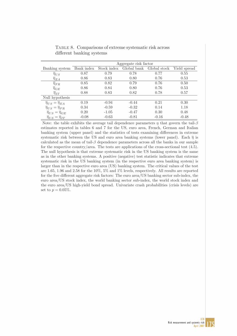
175ECB
Risk measurement and systemic riskApril 2007
Table 8. Comparisons of extreme systematic risk acrossdi erent banking systems
Aggregate risk factor
Banking system Bank index Stock index Global bank Global stock Yield spread
0.87 0.79 0.78 0.77 0.55
0.86 0.83 0.80 0.76 0.53
0.85 0.82 0.79 0.76 0.50
0.86 0.84 0.80 0.76 0.53
0.88 0.83 0.82 0.78 0.57
Null hypothesis
= 0.19 -0.94 -0.44 0.21 0.30
= 0.34 -0.59 -0.32 0.14 1.18
= 0.20 -1.05 -0.47 0.30 0.48
= -0.08 -0.63 -0.81 -0.16 -0.48
Note: the table exhibits the average tail dependence parameters that govern the tail-
estimates reported in tables 6 and 7 for the US, euro area, French, German and Italian
banking system (upper panel) and the statistics of tests examining di erences in extreme
systematic risk between the US and euro area banking systems (lower panel). Each is
calculated as the mean of tail- dependence parameters across all the banks in our sample
for the respective country/area. The tests are applications of the cross-sectional test (4.5).
The null hypothesis is that extreme systematic risk in the US banking system is the same
as in the other banking systems. A positive (negative) test statistic indicates that extreme
systematic risk in the US banking system (in the respective euro area banking system) is
larger than in the respective euro area (US) banking system. The critical values of the test
are 1.65, 1.96 and 2.58 for the 10%, 5% and 1% levels, respectively. All results are reported
for the ve di erent aggregate risk factors: The euro area/US banking sector sub-index, the
euro area/US stock index, the world banking sector sub-index, the world stock index and
the euro area/US high-yield bond spread. Univariate crash probabilities (crisis levels) are
set to = 0 05%.

176ECBRisk measurement and systemic riskApril 2007
Table 9. Domestic and cross-border extreme spilloverrisk among euro area banks: Time variation
Largest bank 1 2 3 4 5
Conditioning banks: German
Germany 3/31/97 (43.5) 8/1/97 (62.0) 4/2/97 (38.4) 8/15/97 (7.2) 7/23/97 (17.3)
Netherlands 3/31/97 (81.1) 4/2/97 (77.9) 4/2/97 (66.2) 8/21/97 (16.9) 4/2/97 (7.3)
France 7/23/97 (25.6) 8/1/97 (37.5) 9/9/97 (41.2) 7/23/97 (19.3) 8/15/97 (8.4)
Spain 7/21/97 (68.8) 5/27/97 (39.7) 5/29/97 (55.9) 7/23/97 (18.9) 8/14/97 (5.5)
Italy 7/21/97 (49.2) 9/9/97 (46.2) 9/9/97 (41.4) 8/21/97 (20.2) 8/21/97 (9.3)
Belgium 8/21/97 (62.2) 4/2/97 (50.1) 3/27/97 (56.7) 7/23/97 (25.9) 6/12/98 (6.9)
Ireland 8/20/97 (43.0) 10/16/97 (24.3) 8/15/97 (21.9) 8/14/97 (11.3) 8/15/97 (4.7)
Portugal 9/9/97 (27.5) 1/14/94 (37.1) 1/25/94 (50.1) 7/23/97 (23.2) 7/23/97 (7.5)
Finland 10/16/97 (30.5) 10/16/97 (26.3) 5/23/94 (37.2) 8/22/97 (23.6) 7/23/97 (9.6)
Greece 3/27/97 (64.0) 3/27/97 (58.8) 4/2/97 (47.8) 3/27/97 (18.8) 8/15/97 (7.4)
Conditioning banks: French
France 2/15/02 (25.3) 9/19/00 (32.8) 6/17/94 (22.5)
Germany 10/9/00 (52.6) 11/21/00 (36.3) 5/21/96 (4.4)
Netherlands 10/10/00 (54.4) 9/20/00 (44.9) 10/22/97 (39.0)
Italy 1/11/02 (20.1) 1/31/01 (37.8) 10/22/97 (32.5)
Spain 10/10/00 (34.3) 9/19/00 (40.6) 10/13/97 (32.1)
Belgium 9/1/00 (47.7) 11/27/01 (52.4) 6/9/98 (40.8)
Ireland 9/20/00 (13.8) 11/21/00 (19.4) 12/7/01 (12.2)
Portugal 1/25/02 (24.8) 1/29/02 (30.4) 10/22/97 (20.4)
Finland 4/14/00 (6.1) 5/31/94 (26.0) 11/4/96 (27.5)
Greece 6/11/98 (15.5) 2/28/97 (32.5) 2/28/97 (19.2)
Conditioning banks: Italian
Italy 9/30/97 (5.4) 9/25/ 97 (9.0) 9/30/97 (3.6)
Germany 7/25/97 (23.9) 7/25/97 (31.7) 10/8/97 (18.8)
Netherlands 10/7/97 (16.6) 8/1/97 (27.7) 8/7/97 (18.7)
Spain 6/27/97 (7.6) 7/14/97 (19.9) 9/9/97 (12.1)
France 10/8/97 (9.9) 10/22/97 (8.3) 9/9/97 (7.9)
Belgium 7/31/97 (25.8) 8/1/97 (44.8) 10/8/97 (30.2)
Ireland 8/22/97 (4.9) 10/8/97 (7.0) 8/7/97 (6.7)
Portugal 8/1/97 (9.1) 8/1/97 (18.2) 8/7/97 (13.6)
Finland - 7/25/97 (8.5) 10/24/97 (5.9)
Greece 9/9/97 (15.3) 10/17/97 (19.2) 8/15/97 (13.4)
Conditioning banks: Spanish
Spain 7/16/97 (33.1) 7/16/97 (4.0)
Germany 3/17/97 (88.0) 5/21/97 (9.0)
Netherlands 7/21/97 (39.0) 7/3/97 (7.3)
France 10/22/97 (34.6) 5/27/97 (5.4)
Italy 7/28/97 (33.2) 6/18/97 (3.8)
Belgium 7/17/97 (47.7) 2/25/97 (12.4)
Ireland 7/16/97 (22.7) -
Portugal 6/16/97 (42.7) 3/31/97 (12.8)
Finland 10/24/97 (21.3) 7/23/97 (3.9)
Greece 6/2/97 (37.9) 3/27/97 (12.4)
Note: The table reports the results of tests examining the structural stability of the extreme spillover
risks documented in table 3. This is done by testing for the constancy of the tail dependence
parameters (null hypothesis) that govern the spillover probabilities in table 3. Applying the recursive
test (4.1) through (4.4) by Quintos et al. (2001), each cell shows the endogenously found break date
and the test value in parentheses. Dates are denoted XX/YY/ZZ, where XX=month, YY=day and
ZZ=year. The critical values of the test are 1.46, 1.78 and 2.54 for the 10%, 5% and 1% levels,
respectively. A test value exceeding these numbers implies an increase in extreme dependence over
time. The absence of a break over the sample period is marked with a dash.

177ECB
Risk measurement and systemic riskApril 2007
Table 10. Multivariate extreme spillover risk amongeuro area and US banks: Time variation
Country/Area Full sample Sub-sample estimates Second sub-sample break tests
break test b1 b2 Endogenous Exogenous
United States ( =25) 11/22/95 (18.5) 0.20 0.41 3/11/97 (2.2) n.a.
Euro area ( =25) 12/5/96 (4.9) 0.13 0.20 (B) 1/18/99 (3.2) (1.4)
Germany ( =6) 7/23/97 (17.6) 0.24 0.52 - (1.9)
(B) 4/2/97 (2.1) (B) 1/22/99 (3.9)
France ( =4) 6/17/94 (21.9) 0.19 0.52 12/7/01 (12.8) (-3.0)
(B) 5/21/96 (4.3) (B) 2/24/97 (3.0)
Italy ( =4) 09/30/97 (3.4) 0.45 0.72 (B) 4/11/03 (2.2) (2.1)
Note: The table reports tests and estimations assessing time variation in the multivariate spillover
probabilities of table 5. The column on the left displays estimated break dates and values from the
recursive Quintos et al. (2001) test (4.1) through (4.4) applied to the parameter governing the
extreme tail dependence of the banks located in the countries/areas displayed on the extreme left.
Dates are denoted XX/YY/ZZ, where XX=month, YY=day and ZZ=year. The forward recursive
version of the test is used, unless marked otherwise. (B) marks the backward recursive version of
the test. The critical values of the test are 1.46, 1.78 and 2.54 for the 10%, 5% and 1% levels,
respectively. The middle columns show pre- and post-break estimates for . The columns on the
right display two tests that assess the occurrence of further breaks in the second half of the sample.
The rst one is the same as the one on the left-hand side. The second one is a simple di erences-
in-means test based on (4.5). The exogenous break point is chosen to be 1/1/99, the time of the
introduction of the euro. Critical values for this test are 1.65, 1.96 and 2.58 for the 10%, 5% and
1% signi cance levels. Note that values for countries/areas with di erent numbers of banks may
not be comparable.

178ECBRisk measurement and systemic riskApril 2007
Figure 1. Evolution of multivariate extreme spilloverrisk among euro area and US banks
0.2
0.3
0.4
0.5
0.6
10/07/93 8/07/97 6/07/01
original declustered
recursive tail dependence estimates for US (N=25)
0.2
0.3
0.4
0.5
0.6
10/07/93 8/07/97 6/07/01
original declustered
recursive tail dependence estimates for EMU (N=25)
0.2
0.3
0.4
0.5
0.6
10/07/93 8/07/97 6/07/01
original declustered
recursive tail dependence estimates for Germany (N=6)
0.2
0.3
0.4
0.5
0.6
10/07/93 8/07/97 6/07/01
original declustered
recursive tail dependence estimates for France (N=4)
0.2
0.3
0.4
0.5
0.6
0.7
10/07/93 8/07/97 6/07/01
orginal declustered
recursive tail dependence estimates for Italy (N=4)

179ECB
Risk measurement and systemic riskApril 2007
Figure 2. Comparisons of the evolution of extremebank spillover risk across countries
0
2
4
6
8
10
4/03/92 2/02/96 12/03/99 10/03/03
original declustered
US vs. EMU
-6
-4
-2
0
2
4
4/03/92 2/02/96 12/03/99 10/03/03
original declustered
US vs. GE
-6
-4
-2
0
2
4
4/03/92 2/02/96 12/03/99 10/03/03
original declustered
US vs. FR
-7
-6
-5
-4
-3
-2
-1
4/03/92 2/02/96 12/03/99 10/03/03
original declustered
US vs. IT

180ECBRisk measurement and systemic riskApril 2007
Table 11. Extreme systematic risk (tail- s) of euro areabanks: Time variation
Bank Aggregate risk factor
Bank index Stock index Global bank Global stock Yield spread
DEUTSCHE 3/12/97 (45.3) 3/12/97 (57.7) 8/15/97 (53.3) 12/5/96 (86.1) 9/14/00 (153.4)
HYPO 7/21/97 (40.1) 10/22/97 (60.0) 9/9/97 (62.8) 10/22/97 (60.5) 10/4/00 (124.1)
DRESDNER 8/1/97 (69.1) 12/5/96 (53.1) 12/5/96 (48.5) 12/5/96 (59.5) 8/22/00 (44.1)
COMMERZ 7/21/97 (22.8) 3/19/97 (34.8) 8/1/97 (30.4) 8/21/97 (70.4) 10/3/00 (142.7)
BGBERLIN 12/3/96 (7.9) 12/3/96 (10.9) 12/5/96 (11.8) 7/3/97 (19.2) 1/4/01 (496.6)
DEPFA 7/5/96 (33.7) 7/15/96 (37.6) 8/21/97 (19.4) 8/12/97 (33.6) 9/13/00 (97.5)
BNPPAR 8/15/97 (34.7) 7/17/97 (41.1) 10/22/97 (27.5) 8/27/97 (34.0) 9/15/00 (77.3)
CA 10/5/00 (50.4) 9/19/00 (52.7) 10/9/00 (26.6) 9/19/00 (31.7) 7/21/00 (127.3)
SGENER 10/22/97 (40.9) 10/22/97 (35.4) 10/22/97 (37.4) 10/22/97 (42.6) 9/21/00 (114.5)
NATEXIS 12/5/96 (6.0) 12/3/96 (8.5) 8/28/97 (11.0) 8/28/97 (21.1) 9/15/00 (155.1)
INTESA 7/31/97 (25.6) 7/28/97 (39.7) 9/9/97 (14.5) 7/31/97 (24.4) 7/24/00 (183.9)
UNICRED 10/8/97 (23.8) 9/25/97 (14.2) 10/8/97 (18.7) 9/9/97 (18.0) 9/11/00 (123.4)
PAOLO 7/28/97 (52.6) 9/25/97 (51.4) 10/24/97 (43.8) 10/8/97 (58.7) 8/17/00 (218.4)
CAPITA 8/12/97 (17.0) 9/10/97 (15.7) 9/9/97 (13.1) 9/9/97 (16.0) 9/15/00 (170.6)
SANTANDER 7/23/97 (60.3) 5/27/97 (64.0) 8/21/97 (28.3) 10/8/97 (51.5) 9/15/00 (207.3)
BILBAO 10/8/97 (54.0) 10/16/97 (58.7) 10/7/97 (36.2) 10/22/97 (68.7) 9/11/00 (209.3)
BANESP 5/16/97 (6.3) 10/16/97 (5.3) 10/22/97 (2.5) 10/22/97 (2.3) 7/21/00 (29.3)
ING 11/26/96 (43.7) 10/22/96 (36.4) 8/21/97 (57.2) 7/5/96 (51.7) 9/20/00 (186.5)
ABNAMRO 11/26/96 (48.1) 12/5/96 (56.3) 7/4/96 (73.9) 7/4/96 (61.6) 9/15/00 (132.5)
FORTIS 3/17/97 (65.4) 12/10/96 (41.1) 12/10/96 (33.0) 7/17/97 (36.7) 9/15/00 (161.2)
ALMANIJ 3/14/97 (59.4) 1/23/97 (56.7) 1/23/97 (54.5) 8/7/97 (77.1) 9/14/00 (238.2)
ALPHA 2/24/97 (52.7) 2/27/97 (64.5) 1/8/97 (36.6) 2/6/97 (66.1) 9/29/00 (80.7)
BCP 6/16/97 (37.8) 7/3/97 (42.2) 8/26/97 (28.7) 7/17/97 (57.6) 9/15/00 (129.0)
SAMPO 10/16/97 (15.2) 10/24/97 (15.6) 10/24/97 (6.0) 10/16/97 (11.5) 8/16/00 (151.6)
IRBAN 8/12/97 (22.4) 3/12/97 (25.2) 8/21/97 (16.5) 8/20/97 (25.3) 9/29/00 (164.7)
Note: The table reports the results of tests examining the structural stability of the extreme sys-
tematic risks of euro area banks documented in table 6. This is done by testing for the constancy of
the tail dependence parameters (null hypothesis) that govern the tail- s in table 6. Applying the
recursive test (4.1) through (4.4) by Quintos et al. (2001), each cell shows the endogenously found
break date and the test value in parentheses. Dates are denoted XX/YY/ZZ, where XX=month,
YY=day and ZZ=year. The critical values of the test are 1.46, 1.78 and 2.54 for the 10%, 5%
and 1% levels, respectively. A test value exceeding these numbers implies an increase in extreme
dependence over time. The absence of a break over the sample period is marked with a dash.

181ECB
Risk measurement and systemic riskApril 2007
Figure 3. Evolution of extreme systematic risk in theeuro area and the US banking systems
0.4
0.5
0.6
0.7
0.8
0.9
5/03/94 4/02/96 3/03/98 2/01/00 1/01/02 12/02/03
original declustered
tail dependence coefficient for EMU banks w.r.t. EMU global index
0.4
0.5
0.6
0.7
0.8
0.9
5/03/94 4/02/96 3/03/98 2/01/00 1/01/02 12/02/03
original declustered
tail dependence coefficient for US banks w.r.t. US global index
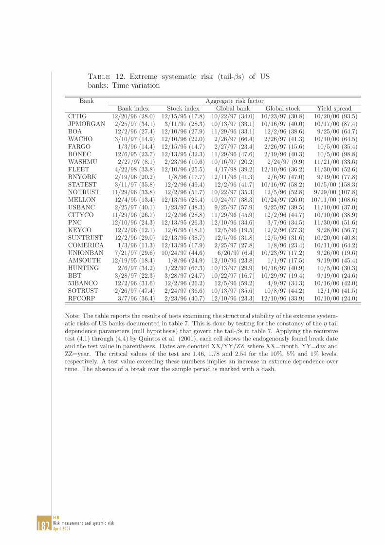
182ECBRisk measurement and systemic riskApril 2007
Table 12. Extreme systematic risk (tail- s) of US
banks: Time variation
Bank Aggregate risk factor
Bank index Stock index Global bank Global stock Yield spread
CITIG 12/20/96 (28.0) 12/15/95 (17.8) 10/22/97 (34.0) 10/23/97 (30.8) 10/20/00 (93.5)
JPMORGAN 2/25/97 (34.1) 3/11/97 (28.3) 10/13/97 (33.1) 10/16/97 (40.0) 10/17/00 (87.4)
BOA 12/2/96 (27.4) 12/10/96 (27.9) 11/29/96 (33.1) 12/2/96 (38.6) 9/25/00 (64.7)
WACHO 3/10/97 (14.9) 12/10/96 (22.0) 2/26/97 (66.4) 2/26/97 (41.3) 10/10/00 (64.5)
FARGO 1/3/96 (14.4) 12/15/95 (14.7) 2/27/97 (23.4) 2/26/97 (15.6) 10/5/00 (35.4)
BONEC 12/6/95 (23.7) 12/13/95 (32.3) 11/29/96 (47.6) 2/19/96 (40.3) 10/5/00 (98.8)
WASHMU 2/27/97 (8.1) 2/23/96 (10.6) 10/16/97 (20.2) 2/24/97 (9.9) 11/21/00 (33.6)
FLEET 4/22/98 (33.8) 12/10/96 (25.5) 4/17/98 (39.2) 12/10/96 (36.2) 11/30/00 (52.6)
BNYORK 2/19/96 (20.2) 1/8/96 (17.7) 12/11/96 (41.3) 2/6/97 (47.0) 9/19/00 (77.8)
STATEST 3/11/97 (35.8) 12/2/96 (49.4) 12/2/96 (41.7) 10/16/97 (58.2) 10/5/00 (158.3)
NOTRUST 11/29/96 (33.8) 12/2/96 (51.7) 10/22/97 (35.3) 12/5/96 (52.8) 9/29/00 (107.8)
MELLON 12/4/95 (13.4) 12/13/95 (25.4) 10/24/97 (38.3) 10/24/97 (26.0) 10/11/00 (108.6)
USBANC 2/25/97 (40.1) 1/23/97 (48.3) 9/25/97 (57.9) 9/25/97 (39.5) 11/10/00 (37.0)
CITYCO 11/29/96 (26.7) 12/2/96 (28.8) 11/29/96 (45.9) 12/2/96 (44.7) 10/10/00 (38.9)
PNC 12/10/96 (24.3) 12/13/95 (26.3) 12/10/96 (34.6) 3/7/96 (34.5) 11/30/00 (51.6)
KEYCO 12/2/96 (12.1) 12/6/95 (18.1) 12/5/96 (19.5) 12/2/96 (27.3) 9/28/00 (56.7)
SUNTRUST 12/2/96 (29.0) 12/13/95 (38.7) 12/5/96 (31.8) 12/5/96 (31.6) 10/20/00 (40.8)
COMERICA 1/3/96 (11.3) 12/13/95 (17.9) 2/25/97 (27.8) 1/8/96 (23.4) 10/11/00 (64.2)
UNIONBAN 7/21/97 (29.6) 10/24/97 (44.6) 6/26/97 (6.4) 10/23/97 (17.2) 9/26/00 (19.6)
AMSOUTH 12/19/95 (18.4) 1/8/96 (24.9) 12/10/96 (23.8) 1/1/97 (17.5) 9/19/00 (45.4)
HUNTING 2/6/97 (34.2) 1/22/97 (67.3) 10/13/97 (29.9) 10/16/97 (40.9) 10/5/00 (30.3)
BBT 3/28/97 (22.3) 3/28/97 (24.7) 10/22/97 (16.7) 10/29/97 (19.4) 9/19/00 (24.6)
53BANCO 12/2/96 (31.6) 12/2/96 (26.2) 12/5/96 (59.2) 4/9/97 (34.3) 10/16/00 (42.0)
SOTRUST 2/26/97 (47.4) 2/24/97 (36.6) 10/13/97 (35.6) 10/8/97 (44.2) 12/1/00 (41.5)
RFCORP 3/7/96 (36.4) 2/23/96 (40.7) 12/10/96 (23.3) 12/10/96 (33.9) 10/10/00 (24.0)
Note: The table reports the results of tests examining the structural stability of the extreme system-
atic risks of US banks documented in table 7. This is done by testing for the constancy of the tail
dependence parameters (null hypothesis) that govern the tail- s in table 7. Applying the recursive
test (4.1) through (4.4) by Quintos et al. (2001), each cell shows the endogenously found break date
and the test value in parentheses. Dates are denoted XX/YY/ZZ, where XX=month, YY=day and
ZZ=year. The critical values of the test are 1.46, 1.78 and 2.54 for the 10%, 5% and 1% levels,
respectively. A test value exceeding these numbers implies an increase in extreme dependence over
time. The absence of a break over the sample period is marked with a dash.

183ECB
Risk measurement and systemic riskApril 2007
Appendix A. Small sample properties of estimators andtests
A.1. Small sample properties of the bivariate estimator. In this
section we investigate the small sample properties of our estimators.
We limit our attention to the bivariate version, which could either be a
spillover probability between two banks or a tail- , and the respective
dependence parameter. Without loss of generality, we will always refer
to tail- below. Three di erent data generating processes are inves-
tigated: The bivariate Pareto distribution, the bivariate Morgenstern
distribution (1956) with Pareto marginals and the bivariate standard
normal distribution. The rst two distributions both have Pareto mar-
ginals, but only the rst distribution exhibits asymptotic dependence
(in which case = 1). The bivariate normal is also asymptoticallyindependent (as long as | | 6= 1). The normal distribution has a depen-dence parameter that varies with the correlation coe cient, and we
investigate di erent con gurations. The precise speci cations of the
distributions are as follows:
1/ Bivariate Pareto
( ) = 1 + ( + 1)
= 1 for 2
= 1.
2/ Bivariate Morgenstern distribution with Pareto marginals
( ) =¡
1¢ ¡
1¢ ¡
1 +¢
1 1
= ( 2)(2 1) 2 for 2
= 1 2
3/ Bivariate normal with correlation coe cient and dependence
parameter
=1 +
2.
The three speci c distributions have the advantage that they allow
us to calculate the true value of and the tail- ( ). Thus, the
estimation bias and asymptotic mean-squared error can be calculated

184ECBRisk measurement and systemic riskApril 2007
explicitly. The true “benchmark” values of the tail- s are:
=¡
2 1¢
(bivariate Pareto),
= (1 + ) 2 2 + 3 (bivariate Morgenstern),
=( )
(bivariate standard normal),
where = { }. In the tables below we evaluate the tail- s anddependence parameters at = 0 05% which is one of the marginal sig-ni cance levels we also use in the empirical applications. Two di erent
sample sizes are considered, a truly small sample of 500 observations
and a larger sample of 3,106, corresponding to the actual sample size
in the empirical application to bank stocks.
The following three tables report true values of as well as estimates
of the average, bias and standard deviation of and for 5,000 Monte
Carlo replications. Notice that biases are reported in absolute and not
in percentage terms. Back-of-the-envelope calculations of the relative
(percentage) biases may nevertheless be handy for sake of comparing
the bias across di erent parametrizations but were omitted for sake
of space considerations.35 Averages, biases and standard deviations
are multiplied with 100 for sake of convenience. The estimates are
conditioned on cuto points that minimize the Asymptotic Mean
Squared error (AMSE). The AMSE is calculated for 5,000 Monte Carlo
replications.36
We start with an evaluation for the Morgenstern distribution with
Pareto marginals (see table A.1).
[Insert table A.1 about here]
Analytic tail- values are small which makes this model the least
realistic as a benchmark for comparison with the tail- we found in
practice. We let both the tail index and the parameter vary. The
table shows that the Morgenstern bias in and does depend on but
not on This is not surprising given that does not enter the analytic
expression of the Morgenstern tail- i.e. the tail- is independent from
35Relative or percentage measures of the bias can be calculated as
100× ( (b) ) and 100× ( (b ) ) for the tail dependence parameter
and the tail- respectively.36If two (unit Pareto) random variables are independent, we previously noted
that { } = 2 with = { } = { } This exact Pareto
tail allows the use of all extreme observations in estimation because of the unbi-
asedness of the Hill statistic under the Pareto law, i.e., = 1

185ECB
Risk measurement and systemic riskApril 2007
marginal properties in this case.37 Biases are small for small but
become substantial in both absolute and relative terms when is large.
Also, the estimation accuracy - as re ected by the standard errors s.e.
- is found to be higher for small values of
Next we turn to the results for the Pareto distribution. The results
are in table A.2.
[Insert table A.2 about here]
In contrast to table A.1, there now appears a considerable downward
bias in absolute terms for both and However, the relative (per-
centage) biases can be shown to be smaller than in the Morgenstern
case. Recall that the true value of is equal to the boundary of 1 in
this case, so that in any empirical exercise one expects at least some
downward bias. Moreover, (absolute and relative) biases and standard
errors decreases with a decrease in correlation (an increase in ).Lastly, we consider the small sample performance for the bivariate
normal distribution (see table A.3).
[Insert table A.3 about here]
For the normal distribution the estimators appear to behave quite rea-
sonably. Absolute and relative biases are found to be smaller than in
the Pareto case. Moreover, it may be di cult to distinguish the normal
distribution from the Pareto distribution just on the basis of, say, the
dependence parameter estimate. To this end it would be helpful to
investigate the tail properties of the marginals as well.
A.2. Small sample properties of the endogenous break test. In
this part of the appendix we investigate the small sample properties
of the recursive test for a single endogenous break in . This is done
through a simulation study in which we use the bivariate normal as the
data-generating process (see table A.4).
[Insert table A.4 about here]
Recall that in this case = (1 + ) 2. By changing the correlationcoe cient, we can easily change the dependence parameter .
The breaks are engineered at ve di erent points in the sample (see
-columns in the table). Three di erent combinations of pre and post-
break s are considered (see rows of the table). The sample size is
3,000. The table shows that the test has more di culty in accurately
locating the break if it is close to the start or the end of the sample.
The reason is that in these cases one has fewer observations available
for one of the two sub-samples. When the change in the dependence
37It can be easily shown that the analytic expressions for Morgenstern bias and
AMSE do not depend on the marginal distributional properties like scale and tail
indices.
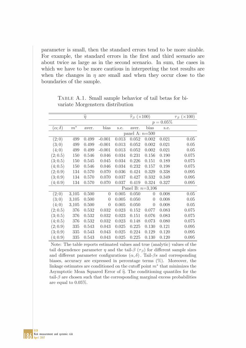
186ECBRisk measurement and systemic riskApril 2007
parameter is small, then the standard errors tend to be more sizable.
For example, the standard errors in the rst and third scenario are
about twice as large as in the second scenario. In sum, the cases in
which we have to be more cautious in interpreting the test results are
when the changes in are small and when they occur close to the
boundaries of the sample.
Table A.1. Small sample behavior of tail betas for bi-variate Morgenstern distribution
b b (×100) (×100)= 0 05%
( ; ) aver. bias s.e. aver. bias s.e.
panel A: =500
(2; 0) 499 0.499 -0.001 0.013 0.052 0.002 0.021 0.05
(3; 0) 499 0.499 -0.001 0.013 0.052 0.002 0.021 0.05
(4; 0) 499 0.499 -0.001 0.013 0.052 0.002 0.021 0.05
(2; 0 5) 150 0.546 0.046 0.034 0.231 0.156 0.190 0.075
(3; 0 5) 150 0.545 0.045 0.034 0.226 0.151 0.189 0.075
(4; 0 5) 150 0.546 0.046 0.034 0.232 0.157 0.198 0.075
(2; 0 9) 134 0.570 0.070 0.036 0.424 0.329 0.338 0.095
(3; 0 9) 134 0.570 0.070 0.037 0.427 0.332 0.349 0.095
(4; 0 9) 134 0.570 0.070 0.037 0.419 0.324 0.327 0.095
Panel B: =3,106
(2; 0) 3,105 0.500 0 0.005 0.050 0 0.008 0.05
(3; 0) 3,105 0.500 0 0.005 0.050 0 0.008 0.05
(4; 0) 3,105 0.500 0 0.005 0.050 0 0.008 0.05
(2; 0 5) 376 0.532 0.032 0.023 0.152 0.077 0.083 0.075
(3; 0 5) 376 0.532 0.032 0.023 0.151 0.076 0.083 0.075
(4; 0 5) 376 0.532 0.032 0.023 0.148 0.073 0.080 0.075
(2; 0 9) 335 0.543 0.043 0.025 0.225 0.130 0.121 0.095
(3; 0 9) 335 0.543 0.043 0.025 0.224 0.129 0.120 0.095
(4; 0 9) 335 0.543 0.043 0.025 0.225 0.130 0.120 0.095
Note: The table reports estimated values and true (analytic) values of the
tail dependence parameter and the tail- ( ) for di erent sample sizes
and di erent parameter con gurations ( ) Tail- and corresponding
biases, accuracy are expressed in percentage terms (%). Moreover, the
linkage estimates are conditioned on the cuto point that minimizes the
Asymptotic Mean Squared Error of b The conditioning quantiles for the
tail- are chosen such that the corresponding marginal excess probabilities
are equal to 0.05%.

187ECB
Risk measurement and systemic riskApril 2007
Table A.2. Small sample behavior of tail betas for bi-variate Pareto distribution
b b ( ) (×100) ( ) (×100)= 0 05%
aver. bias s.e. aver. bias s.e.
Panel A: =500
2 31 0.831 -0.169 0.113 15.44 -10.12 13.15 25.57 1
3 26 0.763 -0.237 0.126 8.33 -5.79 9.49 14.11 1
4 22 0.719 -0.280 0.134 5.49 -3.04 7.40 8.53 1
indep. 499 0.498 0 0.013 0.05 0 0.02 0.05 1/2
Panel B: =3,106
2 89 0.889 -0.111 0.073 19.19 -6.38 8.73 25.57 1
3 45 0.832 -0.168 0.106 10.61 -3.50 7.51 14.11 1
4 42 0.777 -0.222 0.110 6.28 -2.25 5.37 8.53 1
indep. 3,105 0.500 0 0.005 0.05 0 0 0.05 1/2
Note: The table reports estimated values and true (analytic) values of the tail
dependence parameter and the tail- ( ) for di erent sample sizes and di erent
values of Tail- and corresponding biases, accuracy are expressed in percentage
terms (%). Moreover, the linkage estimates are conditioned on the cuto point
that minimizes the Asymptotic Mean Squared Error of b The conditioning
quantiles for the tail- are chosen such that the corresponding marginal excess
probabilities are equal to 0.05%.
Table A.3. Small sample behavior of tail betas for bi-variate normal distribution
b b (×100) (×100) = 1+2
= 0 05%aver. bias s.e. aver. bias s.e.
panel A: =500
3 4 138 0.795 -0.080 0.038 13.55 -4.59 5.11 18.14 0.875
1 2 154 0.684 -0.065 0.038 3.09 -1.12 1.69 4.21 0.75
1 4 233 0.583 -0.042 0.026 0.47 -0.19 0.27 0.67 0.625
0 499 0.499 -0.001 0.013 0.05 0 0.02 0.05 0.5
Panel B: =3,106
3 4 299 0.815 -0.060 0.031 15.74 -2.40 4.10 18.14 0.875
1 2 403 0.699 -0.051 0.027 3.47 -0.74 1.20 4.21 0.75
1 4 574 0.594 -0.031 0.020 0.54 -0.12 0.20 0.67 0.625
0 3105 0.500 0 0.005 0.05 0 0 0.05 0.5
Note: The table reports estimated values and true (analytic) values of the tail
dependence parameter and the tail- ( ) for di erent sample sizes and di erent
correlations Tail- and corresponding biases, accuracy are expressed in per-
centage terms (%). Moreover, the linkage estimates are conditioned on the cuto
point that minimizes the Asymptotic Mean Squared Error of b The condition-
ing quantiles for the tail- are chosen such that the corresponding marginal excess
probabilities are equal to 0.05%.

188ECBRisk measurement and systemic riskApril 2007
Table A.4. Simulated breakpoints
Estimated breakpoints
(standard error)
( 1; 2) r=1/3 r=1/2 r=2/3
(0 5; 0 7) 0.364 0.514 0.617
(0.190) (0.166) (0.117)
(0 5; 0 9) 0.264 0.485 0.636
(0.095) (0.078) (0.092)
(0 7; 0 9) 0.394 0.508 0.587
(0.209) (0.172) (0.194)
Note: Estimated breakpoints are reported for the tail dependence parameter of
the bivariate normal df. The break estimates are reported for varying locations of
the true breakpoints (r=1/3,1/2,2/3). The number of Monte Carlo replications is
set to 1,000. The accompanying sampling errors are reported between brackets.
Q-tests are calculated starting with a minimum sample size of 500. For sake of
convenience, we set the number of upper order extremes used in estimating the tail
index equal to 2 2 3

189ECB
Risk measurement and systemic riskApril 2007
Appendix B List of banks in the sampleTable B.1: List of banks in the sample
Euro area United States
Bank name Abbreviation Bank name Abbreviation
Germany Citigroup CITIG
Deutsche Bank DEUTSCHE JP Morgan Chase JP MORGAN
Bayerische Hypo- und Vereinsbank HYPO Bank of America BOA BAMERICA
Dresdner Bank DRESDNER Wachovia Corporation WACHOVIA
Commerzbank COMMERZ Wells Fargo and Company FARGO
Bankgesellschaft Berlin BGBERLIN Bank One Corporation BONE
DePfa Group DEPFA Washington Mutual Inc WASHING
France Fleet Boston Financial Corporation FLEET
BNP Paribas BNPPAR Bank of New York BNYORK
Crédit Agricole CA State Street SSTREET
Societe Generale SGENER Northern Trust NTRUST
Natexis Banques Populaires NATEXIS Mellon MELLON
Italy US Bancorp BCORP
Banca Intesa INTESA National City Corporation CITYCO
UniCredito Italiano UNICREDIT PNC Financial Services Group PNC
Sanpaolo IMI PAOLO Keycorp KEYCO
Capitalia CAPITA Sun Trust SUTRUST
Spain Comerica Incorporated COMERICA
Banco Santander Central Hispano SANTANDER Unionbancal Corporation UNIONBANK
Banco Bilbao Vizcaya Argentaria BILBAO AmSouth Bancorp AMSOUTH
Banco Espagnol de Credito BANESP Huntington Bancshares Inc HUNTING
Netherlands BBT Corporation BBT
ABN AMRO ABNAMRO Fifth Third Bancorp 53BANCO
ING Bank ING Southtrust SOTRUST
Belgium Regions Financial Corporation REGIONS
Fortis FORTIS
Almanij ALMANIJ
Finland
Sampo Leonia SAMPO
Greece
Alpha Bank ALPHA
Ireland
Allied Irish Banks IRBAN
Portugal
Banco Commercial Portugues BCP

190ECBRisk measurement and systemic riskApril 2007
Ap
pen
dix
C:
Bal
ance
sh
eet
dat
a
Tab
le C
.1: T
otal
ass
ets
of e
uro
area
ban
ks (
mill
ion
US
$)
Ban
k N
ame
2003
2002
2001
2000
1999
1998
1997
1996
1995
1994
1993
1992
Ave
rag
eA
vera
ge
1998
-200
3A
vera
ge
1992
-199
7
DE
UT
SC
HE
93
4,43
473
0,30
164
1,82
664
7,18
656
9,12
755
5,44
641
9,89
238
6,64
546
1,18
035
2,74
030
8,79
029
7,20
052
5,39
767
9,72
037
1,07
5
BN
PP
AR
988,
881
744,
867
727,
318
644,
886
700,
675
378,
990
339,
817
355,
299
325,
880
271,
640
250,
440
275,
310
500,
334
697,
603
303,
064
CA
1,
105,
378
609,
055
496,
421
498,
433
441,
524
455,
781
419,
971
477,
591
387,
130
328,
130
282,
870
292,
090
482,
864
601,
099
364,
630
AB
NA
MR
O
707,
801
583,
073
526,
450
505,
419
460,
000
504,
122
414,
655
343,
699
340,
640
290,
800
252,
990
246,
980
431,
386
547,
811
314,
961
HY
PO
597,
584
552,
068
631,
216
646,
016
485,
099
521,
336
453,
909
n.a.
203,
960
173,
600
151,
150
134,
300
413,
658
572,
220
223,
384
SG
EN
ER
68
1,21
652
5,78
945
1,66
042
4,19
843
7,55
844
7,48
641
0,65
533
9,58
632
6,67
027
7,55
025
9,79
025
1,32
040
2,79
049
4,65
131
0,92
9
DR
ES
DN
ER
602,
461
433,
489
446,
238
449,
036
397,
944
424,
620
372,
779
n.a.
330,
340
252,
180
215,
190
199,
820
374,
918
458,
965
274,
062
CO
MM
ER
Z
481,
653
442,
333
441,
510
422,
867
371,
134
374 ,
896
294,
671
n.a.
275,
700
217,
640
162,
120
142,
130
329,
696
422,
399
218,
452
ING
68
4,0 0
450
0,32
639
0,72
537
8,14
935
1,23
432
6,81
319
0,26
917
9,93
315
4,05
012
5,33
010
5,88
010
9,54
029
1,35
443
8,54
214
4,16
7
INT
ES
A
327,
353
290,
917
275,
967
308,
334
309,
719
330,
138
158,
597
163,
712
n.a.
n.a.
n.a.
n.a.
270,
592
307,
071
161,
154
FO
RT
IS
536,
857
396,
107
327,
451
309,
011
330,
835
333,
608
n.a.
n.a.
19,6
5016
,690
14,2
2014
,520
229,
895
372,
312
16,2
70
BIL
BA
O
356,
921
288,
311
269,
2 08
272,
225
236,
802
235,
799
214,
978
213,
680
115,
820
98,8
2081
,420
87,6
4020
5,96
927
6,54
413
5,39
3
UN
ICR
ED
IT
300,
652
226,
638
188,
380
188,
565
169,
705
175,
346
161,
206
n.a.
n.a.
n.a.
n.a.
n.a.
201,
499
208,
214
161,
206
BG
BE
RLI
N
191,
936
182,
046
165,
227
189,
389
192,
212
217,
785
195,
372
206,
377
34,0
6020
,650
n.a.
n.a.
159,
505
189,
766
114,
115
SA
NT
AN
DE
R25
0,90
418
8,02
415
9,50
516
0,32
5n.
a.n.
a.n.
a.n.
a.13
5,06
011
3,92
073
,120
61,3
1014
2,77
118
9,68
995
,853
CA
PIT
A
159,
915
146,
148
115,
815
123,
504
134,
397
142,
745
114,
969
140,
831
n.a.
n.a.
n.a.
n.a.
134,
790
137,
087
127,
900
ALM
AN
IJ
327,
898
265,
080
228,
521
202,
453
187,
390
198,
213
187,
745
740
3,30
02,
810
2,37
01,
310
133,
986
234,
926
33,0
46
DE
PF
A
219,
708
152,
944
159,
425
n.a.
n.a.
n.a.
n.a.
n.a.
103,
580
76,8
0062
,850
56,1
5011
8,77
917
7,35
974
,845
NA
TE
XIS
171,
646
139,
891
97,2
5410
5,26
894
,861
49,5
5849
,972
110,
159
n.a.
n.a.
n.a.
n.a.
102,
326
109,
746
80,0
6 6
IRB
AN
98,6
9987
,717
76,5
5172
,516
65,5
4861
,439
52,8
1543
,105
37,8
1032
,200
29,4
3029
,940
57,3
1477
,078
37,5
50
BA
NE
SP
72,9
2351
,919
39,3
8441
,296
39,9
5842
,800
36,6
0642
,715
41,7
6043
,120
53,2
1061
,750
47,2
8748
,047
46,5
27
BC
P85
,483
64,8
6155
,479
57,5
5235
,211
33,9
5529
,662
n.a.
36,1
7013
,960
10,9
0010
,370
39,4
1855
,423
20,2
12
SA
MP
O21
,454
18,2
5515
,126
n.a.
n.a.
n.a.
n.a.
n.a.
n.a.
n.a.
n.a.
n.a.
18,2
7818
,278
n.a.
ALP
HA
38,9
0230
,123
26,0
5228
,420
25,4
4516
,372
12,4
0911
,680
9,25
07,
130
5,61
05,
0 20
18,0
3427
,552
8,51
7
PA
OLO
8,80
77,
073
5,58
66,
133
5,37
56,
056
5,16
34,
791
4,64
34,
100
3,72
94,
608
5,50
56,
505
4,50
6
Su
m9,
953,
470
7,65
7,35
36,
958,
293
6,68
1,18
26,
041,
753
5,83
3,30
44,
536,
112
3,02
0,54
33,
346,
653
2,71
9,81
02,
326,
079
2,28
1,30
85,
638,
347
7,34
8,60
83,
641,
882
Not
es: B
NP
PA
RIB
AS
unt
il 19
95 B
NP
. Ban
ks a
re o
rder
ed in
dec
linin
g si
ze o
f ave
rage
ass
ets
over
the
sam
ple
perio
d. n
.a. m
eans
dat
a no
t ava
ilabl
e.
Dat
a so
urce
: Ban
ksco
pe a
nd o
wn
calc
ulat
ions
.

191ECB
Risk measurement and systemic riskApril 2007
Ap
pen
dix
C:
Bal
ance
sh
eet
dat
a
Tab
le C
.2: T
otal
ass
ets
of U
S b
anks
(m
illio
n U
S$)
Ban
k N
ame
2003
2002
2001
2000
1999
1998
1997
1996
1995
1994
1993
1992
Ave
rag
eA
vera
ge
1998
-200
3A
vera
ge
1992
-199
7
CIT
IG
1,26
4,03
21,
097,
190
1,05
1,45
090
2,21
071
6,93
766
8,64
1n.
a.n.
a.22
0,11
021
0,48
717
5,71
216
3,84
664
7,06
295
0,07
719
2,53
9
JP M
OR
GA
N77
0,91
275
8,80
069
3,57
571
5,34
840
6,10
536
5,87
536
5,52
133
6,09
918
4,87
915
4,91
713
3,88
810
2,94
141
5,73
861
8,43
621
3,04
1
BA
ME
RIC
A73
6,44
566
0,45
862
1,76
464
2,19
163
2,57
461
7,67
926
4,56
218
5,79
416
3,39
814
7,67
013
6,69
313
3,44
941
1,89
065
1,85
217
1,92
8
BO
NE
326,
563
277,
383
268,
954
269,
300
269,
425
261,
496
115,
901
101,
848
n.a.
n.a.
n.a.
n.a.
236,
359
278,
854
108,
875
FA
RG
O
387,
798
349,
259
307,
569
272,
426
218,
102
202,
475
88,5
4080
,175
50,3
1653
,374
52,5
1352
,537
176,
257
289,
605
62,9
09
WA
CH
OV
IA40
1,03
234
1,83
933
0,45
274
,032
67,3
5364
,123
65,3
9746
,886
44,9
6439
,171
36,5
1433
,356
128,
760
213,
138
44,3
82
FLE
ET
20
0,3 5
619
0,58
920
3,63
817
9,51
919
0,69
210
4,55
485
,690
85,5
5511
,037
9,75
78,
246
8,28
810
6,49
317
8,22
534
,762
BC
OR
P
189,
286
180,
027
171,
390
87,3
3681
,530
76,4
3871
,295
36,4
8931
,865
21,7
8421
,458
20,7
7382
,473
131,
001
33,9
44
CIT
YC
O11
3,93
411
8,25
810
5,81
788
,535
87,1
2288
,246
54,6
8450
,856
36,1
9932
,114
31,0
6828
,964
69,6
4910
0,31
838
,981
KE
YC
O84
,147
84,7
1080
,400
87,1
6583
,344
79,9
6673
,625
67,6
8866
,339
66,7
9832
,648
25,4
5769
,357
83,2
8955
,426
PN
C
68,1
9366
,410
69,5
7069
,916
75,4
2877
,232
75,1
0173
,174
73,5
0764
,221
61,9
4551
,523
68,8
5271
,12 5
66,5
78
BN
YO
RK
89,2
5874
,948
78,0
1974
,266
71,7
9560
,078
56,1
5452
,121
42,7
1239
,287
36,0
8836
,644
59,2
8174
,727
43,8
34
SS
TR
EE
T80
,435
79,6
2165
,410
64,6
4456
,226
43,1
8537
,450
31,3
9025
,785
21,7
4418
,720
16,4
9045
,092
64,9
2025
,263
SO
TR
US
T
51,8
8550
,570
48,8
5045
,170
43,2
0338
,054
30,7
1513
,339
n.a.
n.a.
n.a.
n.a.
40,2
2346
,288
22,0
27
BB
T
90,4
6780
,217
70,8
7059
,340
43,4
8134
,427
29,1
7821
,247
15,9
929,
179
7,79
46,
256
39,0
3763
,134
14,9
41
53B
AN
CO
91,1
4380
,899
71,0
2645
,857
41,5
9028
,922
21,3
7520
,549
17,0
5714
,973
11,9
8110
,232
37,9
6759
,906
16,0
28
ME
LLO
N
20,8
3926
,841
27,8
1341
,974
39,6
1942
,235
38,8
0237
,339
40,7
3438
,716
36,0
5031
,541
35,2
0933
,220
37,1
97
CO
ME
RIC
A
52,6
8439
,643
37,2
5633
,697
31,2
4329
,375
28,9
3627
,052
28,3
9427
,044
24,9
3522
,364
31,8
8537
,317
26,4
54
RE
GIO
NS
48,8
8147
,939
45,3
8343
,688
42,7
1436
,832
23,0
3418
,930
13,7
0912
,839
10,4
767,
881
29,3
5944
,240
14,4
78
UN
ION
BA
NK
42,4
8840
,193
36,0
7835
,170
33,6
8532
,301
30,6
1229
,304
19,5
1816
,761
16,3
9116
,844
29,1
1236
,652
21,5
72
AM
SO
UT
H
45,6
7040
,598
38,6
2238
,968
43,4
2719
,919
18,6
5718
,440
17,7
4016
,845
12,5
849,
790
26,7
7237
,867
15,6
76
WA
SH
ING
29,3
2726
,723
31,6
3934
,715
35,0
3632
,466
26,0
7021
,241
21,6
3318
,458
15,8
27n.
a.26
,649
31,6
5120
,646
HU
NT
ING
30
,566
27,7
0228
,497
28,5
9929
,037
28,2
9626
,731
20,8
5220
,255
17,7
7117
,619
16,2
4724
,347
28,7
8319
,912
NT
RU
ST
33
,403
31,9
7432
,758
29,7
0923
,500
23,3
0421
,185
18,1
2715
,231
14,7
3613
,538
11,9
0722
,448
29,1
0815
,787
SU
TR
US
Tn.
a.4,
638
3,99
13,
459
3,50
43,
478
2,29
2n.
a.46
,472
42,5
3440
,728
36,6
4718
,774
3,81
433
,735
Su
m5,
249,
743
4,77
7,43
04,
520,
789
3,96
7,23
53,
366,
670
3,05
9,59
61,
651,
505
1,39
4,49
31,
207,
844
1,09
1,17
995
3,41
684
3,97
52,
879,
044
4,15
7,54
61,
350,
913
Not
es: C
omer
ica
until
199
5 C
omer
ica
Det
roit.
Ban
ks a
re o
rder
ed in
dec
linin
g si
ze o
f ave
rage
ass
ets
over
the
sam
ple
perio
d. n
.a. m
eans
dat
a no
t ava
ilabl
e.D
ata
sour
ce: B
anks
cope
and
ow
n ca
lcul
atio
ns.

192ECBRisk measurement and systemic riskApril 2007
Ap
pen
dix
C:
Bal
ance
sh
eet
dat
a
Tab
le C
.3: D
ue fr
om b
anks
for
euro
are
a ba
nks
(mill
ion
US
$)
Ban
k N
ame
2003
2002
2001
2000
1999
1998
1997
1996
1995
1994
1993
1992
Ave
rag
e A
vera
ge
1998
-200
3 A
vera
ge
1992
-199
7
BN
PP
AR
20
5,79
715
3,64
116
4,46
912
1,53
616
0,51
083
,169
82,1
4710
3,73
596
,870
77,9
2072
,780
87,3
7011
7,49
514
8,18
786
,804
DE
UT
SC
HE
18
0,57
014
7,22
613
6,05
913
5,62
413
4,23
512
4,20
410
0,11
999
,183
77,0
6063
,300
54,8
6056
,490
109,
078
142,
986
75,1
69
CA
11
9,53
470
,083
56,0
5261
,259
62,2
7579
,898
78,6
9911
2,65
698
,490
78,0
4068
,290
63,2
5079
,044
74,8
5083
,237
DR
ES
DN
ER
15
4,86
292
,666
68,2
7683
,419
56,9
3477
,022
68,8
36n.
a.55
,910
40,8
3029
,470
32,3
0069
,139
88,8
6345
,469
SG
EN
ER
76
,133
56,9
9956
,004
50,4
0955
,263
77,4
9989
,485
66,6
6972
,850
66,7
2061
,240
62,9
1066
,015
62,0
5169
,979
AB
NA
MR
O74
,261
43,9
6443
,729
45,2
0547
,419
71,0
4769
,495
68,9
8381
,860
73,2
2065
,820
65,0
8062
,507
54,2
7170
,743
CO
MM
ER
Z
65,1
9 156
,900
55,7
7069
,266
50,0
2667
,994
49,2
10n.
a.59
,180
44,8
8032
,660
23,2
5052
,212
60,8
5841
,836
HY
PO
66,4
8960
,068
78,6
3484
,804
56,0
8967
,207
68,6
370
25,0
0017
,000
18,0
5012
,910
50,4
4468
,882
28,3
19
FO
RT
IS
105,
699
87,8
6057
,640
60,3
0782
,766
68,5
22n.
a.n.
a.2,
150
2,62
02,
530
2,57
047
,266
77,1
322,
468
INT
ES
A
36,6
5731
,916
35,4
0044
,249
44,3
9864
,423
33,9
7534
,586
n.a.
n.a.
n.a.
n.a.
40,7
0142
,841
34,2
81
ALM
AN
IJ
47,7
3539
,979
34,6
6228
,575
27,1
2843
,366
53,8
42n.
a.n.
a.n.
a.n.
a.n.
a.39
,327
36,9
0753
,842
ING
77
,11 5
47,9
0547
,662
41,0
8742
,126
59,5
1626
,071
21,7
8322
,000
16,8
5013
,840
16,3
2036
,023
52,5
6819
,477
BG
BE
RLI
N
35,5
0232
,286
29,6
0635
,579
36,7
3845
,972
43,0
3743
,984
14,3
406,
710
n.a.
n.a.
32,3
7535
,947
27,0
18
UN
ICR
ED
IT
41,4
0430
,915
23,3
1923
,173
20,1
0027
,181
35,0
89n.
a.n.
a.n.
a.n.
a.n.
a.28
,740
27,6
8235
,089
BIL
BA
O
12,1
2912
,371
8,69
119
,582
22,6
2131
,674
41,4
9343
,787
35,4
3031
,930
27,0
3024
,580
25,9
4317
,845
34,0
42
SA
NT
AN
DE
R35
,994
35,6
3029
,007
25,5
13n.
a.n.
a.n.
a.n.
a.28
,570
20,9
9017
,390
12,4
7025
,695
31,5
3619
,855
NA
TE
XIS
54,0
1538
,767
14,6
9414
,853
23,4
227,
821
8,87
420
,808
n.a.
n.a.
n.a.
n.a.
22,9
0725
,595
14,8
41
CA
PIT
A
21,6
2221
,410
17,3
6 015
,500
18,5
9223
,072
23,7
9326
,081
n.a.
n.a.
n.a.
n.a.
20,9
2919
,593
24,9
37
DE
PF
A
23,3
2314
,117
12,3
73n.
a.n.
a.n.
a.n.
a.n.
a.4,
170
4,32
03,
540
4,62
09,
495
16,6
044,
163
BA
NE
SP
5,46
12,
521
1,80
44,
663
4,96
57,
802
6,48
68,
069
10,4
708,
410
7,92
06,
940
6,29
34,
536
8,04
9
IRB
AN
4,06
95,
198
5,82
84,
312
4,12
26,
186
6,27
04,
645
3,95
04,
070
3,74
02,
980
4,61
44,
953
4,27
6
BC
P4,
724
3,51
54,
104
5,53
12,
376
3,56
85,
951
n.a.
7,72
04,
140
2,69
01,
500
4,16
53,
970
4,40
0
ALP
HA
2,13
01,
728
2,56
35,
399
4,23
93,
338
1,59
22,
449
1,54
01,
340
290
390
2,25
03,
233
1,26
7
SA
MP
O1,
284
2,70
71,
790
n.a.
n.a.
n.a.
n.a.
n.a.
n.a.
n.a.
n.a.
n.a.
1,92
71,
927
n.a.
PA
OLO
2,32
31,
681
1,26
21,
528
863
1,69
01,
391
1,23
31,
356
1,22
61,
298
1,57
71,
453
1,55
81,
347
Su
m1,
454,
021
1,09
2,05
398
6,75
798
1,37
295
7,20
81,
042,
172
894,
490
658,
649
698,
916
564,
516
483,
438
477,
507
956,
035
1,10
5,37
579
0,90
6
Not
es: B
NP
PA
RIB
AS
unt
il 19
95 B
NP
. Ban
ks a
re o
rder
ed in
dec
linin
g si
ze o
f ave
rage
am
ount
s du
e fr
om b
anks
ove
r th
e sa
mpl
e pe
riod.
n.a
. mea
ns d
ata
not a
vaila
ble.
D
ata
sour
ce: B
anks
cope
and
ow
n ca
lcul
atio
ns.

193ECB
Risk measurement and systemic riskApril 2007
Ap
pen
dix
C:
Bal
ance
sh
eet
dat
a
Tab
le C
.4: D
ue fr
om b
anks
for
US
ban
ks (
mill
ion
US
$)
Ban
k N
ame
2003
2002
2001
2000
1999
1998
1997
1996
1995
1994
1993
1992
Ave
rag
eA
vera
ge
1998
-200
3A
vera
ge
1992
-199
7
SS
TR
EE
T21
,628
28,1
3320
,306
21,2
8916
,902
12,0
0810
,076
7,56
25,
975
4,84
75,
148
4,80
313
,223
20,0
446,
402
CIT
IG19
,777
16,3
8219
,216
17,2
7413
,429
13,4
25n.
a.n.
a.9,
256
7,20
17,
137
6,24
912
,935
16,5
847,
461
JP M
OR
GA
N10
,17 5
8,94
212
,743
8,33
328
,076
7,21
22,
886
8,34
41,
986
1,36
21,
221
1,51
67,
733
12,5
802,
886
BA
ME
RIC
A8,
051
6,81
35,
932
5,44
84,
838
6,75
02,
395
1,84
35,
899
6,77
12,
956
2,77
95,
040
6,30
53,
774
NT
RU
ST
8,
766
8,26
76,
954
5,19
12,
291
3,26
42,
282
2,06
01,
567
1,86
52,
090
1,86
03,
871
5,78
91,
954
BO
NE
3,09
31,
503
1,03
05,
210
6,64
54,
642
n.a.
n.a.
n.a.
n.a.
n.a.
n.a.
3,68
73,
687
n.a.
BN
YO
RK
7,
154
4,41
85,
924
4,94
96,
208
4,13
41,
343
809
644
854
652
672
3,14
75,
464
829
WA
CH
OV
IA2,
308
3,51
26,
875
3,23
91,
073
2,91
671
031
645
17
1319
01,
801
3,32
128
1
ME
LLO
N
2,77
01,
768
4,08
92,
349
657
991
925
790
553
433
889
992
1,43
42,
104
764
FLE
ET
2,
695
3,67
93,
744
2,82
61,
772
444
7685
80
1,00
00
01,
425
2,52
732
2
UN
ION
BA
NK
235
279
6474
183
210
629
1,13
150
51,
030
1,20
01,
201
562
174
949
PN
C
493
518
413
380
207
174
570
145
139
149
233
695
343
364
322
CIT
YC
O59
261
512
049
129
141
4928
251
9754
31,
234
325
274
376
SU
TR
US
Tn.
a.n.
a.n.
a.n.
a.n.
a.n.
a.n.
a.n.
a.29
5647
669
531
4n.
a.31
4
FA
RG
O
988
352
206
9542
111
347
1,23
810
70
029
036
321
7
BC
OR
P
n.a.
434
625
200
897
7623
850
117
3346
238
446
64
CO
ME
RIC
A
2314
4324
138
126
137
789
71,
231
221
2142
2
KE
YC
O18
611
283
3435
2053
121
745
381
1414
115
078
221
RE
GIO
NS
n.a.
304
667
310
144
3033
470
110
114
226
20
BB
T27
114
811
539
715
271
14
7n.
a.63
108
8
53B
AN
CO
5819
815
210
982
5127
311
111
160
108
12
HU
NT
ING
34
3721
57
103
402
284
313
134
5734
79
WA
SH
ING
1716
2818
1515
n.a.
n.a.
n.a.
n.a.
n.a.
n.a.
1818
n.a.
AM
SO
UT
H
728
1261
2429
00
11
10
1427
0
SO
TR
US
T5
46
10
10
0n.
a.n.
a.n.
a.n.
a.2
30
Su
m89
,325
86,4
7689
,369
77,2
0083
,984
56,8
7522
,881
25,7
3627
,458
26,4
6023
,534
24,4
3757
,064
80,6
5027
,677
Not
es: C
omer
ica
until
199
5 C
omer
ica
Det
roit.
Ban
ks a
re o
rder
ed in
dec
linin
g si
ze o
f ave
rage
am
ount
s du
e fr
om b
anks
ove
r th
e sa
mpl
e pe
riod.
n.a
. mea
ns d
ata
not a
vaila
ble.
D
ata
sour
ce: B
ank s
cope
and
ow
n ca
lcul
atio
ns.

194ECBRisk measurement and systemic riskApril 2007
Ap
pen
dix
D:
Ret
urn
an
d s
pre
ad d
ata
Tab
le D
.1: M
omen
ts o
f eur
o ar
ea r
etur
ns a
nd c
orre
latio
ns w
ith a
ggre
gate
ris
k fa
ctor
s
Ban
kM
ean
Sta
nd
ard
D
evia
tio
nS
kew
nes
sK
urt
osi
sC
orr
elat
ion
, B
ank
ind
exC
orr
elat
ion
, S
tock
ind
exC
orr
elat
ion
, Yie
ld
spre
ad, 1
998-
2004
Co
rrel
atio
n,
Yie
ld s
pre
ad
DE
UT
SC
HE
0.01
2.0
-0.1
4.0
76.8
69.2
-2.8
n.a.
HY
PO
-0.0
12.
40.
16.
165
.757
.1-5
.3n.
a.
DR
ES
DN
ER
0.01
2.1
0.2
5.9
67.2
59.3
-2.8
n.a.
CO
MM
ER
Z
0.00
2.0
0.2
6.9
68.2
62.3
-5.3
n.a.
BG
BE
RLI
N
-0.0
62.
4-1
.432
.820
.417
.6-5
.1n.
a.
DE
PF
A0.
051.
90.
26.
231
.230
.3-5
.5n.
a.
BN
PP
AR
0.
032.
20.
13.
769
.864
.1-1
.3n.
a.
CA
0.
021.
4-0
.821
.329
.625
.7-2
.6n.
a.
SG
EN
ER
0.
042.
20.
13.
972
.766
.1-1
.7n.
a.
NA
TE
XIS
0.
011.
70.
36.
334
.834
.4-2
.7n.
a.
INT
ES
A
0.02
2.5
0.3
2.9
55.5
48.8
-2.9
n.a.
UN
ICR
ED
IT0.
042.
30.
98.
557
.552
.2-1
.0n.
a.
PA
OLO
0.00
2.3
0.2
2.1
65.5
59.5
-4.0
n.a.
CA
PIT
A-0
.04
2.6
0.3
5.2
51.4
46.5
-5.0
n.a.
SA
NT
AN
DE
R0.
042.
1-0
.15.
174
.469
.0-1
.8n.
a.
BIL
BA
O
0.04
2.0
0.0
5.5
76.6
71.4
-1.3
n.a.
BA
NE
SP
-0.0
22.
4-1
4.5
543.
223
.319
.9-6
.4n.
a.
AB
NA
MR
O0.
042.
0-0
.15.
377
.772
.5-1
.3n.
a.
ING
0.04
2.2
-0.1
7.5
76.8
73.7
-3.1
n.a.
FO
RT
IS
0.03
2.0
0.2
8.4
68.3
63.0
-1.3
n.a.
ALM
AN
IJ
0.03
1.6
0.4
5.1
48.3
44.9
-1.9
n.a.
ALP
HA
0.03
2.1
0.4
3.7
23.4
24.3
-6.1
n.a.
BC
P0.
001.
5-0
.212
.239
.437
.6-5
.3n.
a.
SA
MP
O0.
072.
80.
37.
726
.527
.6-2
.5n.
a.
IRB
AN
0.05
1.7
-0.4
7.4
44.5
43.2
1.5
n.a.
PO
OLE
D E
uro
area
0.02
2.1
-0.7
41.2
Ban
k in
dex
0.02
0.5
-0.2
5.6
Sto
ck in
dex
0.02
0.5
-0.3
3.5
Yie
ld s
prea
d, 1
998-
2004
8.05
3.2
0.6
-0.7
Dat
a so
urce
: Dat
astr
eam
and
ow
n ca
lcul
atio
ns.
Not
es: R
etur
ns fo
r in
divi
dual
ban
k st
ocks
are
dai
ly e
xces
s re
turn
s, c
alcu
late
d as
tota
l ret
urn
indi
ces
min
us 1
-mon
th L
IBO
Rs.
Ret
urns
for
indi
ces
are
calc
ulat
ed w
ithou
t su
bstr
actin
g LI
BO
R. M
eans
, sta
ndar
d de
viat
ions
and
cor
rela
tion
coef
ficie
nts
are
in %
. Ret
urn
data
ser
ies
run
from
2 A
pril
1992
to 2
7 F
ebru
ary
2004
. n.a
. mea
ns n
ot

195ECB
Risk measurement and systemic riskApril 2007
Ap
pen
dix
D:
Ret
urn
an
d s
pre
ad d
ata
Tab
le D
.2: M
omen
ts o
f US
ret
urns
and
cor
rela
tions
with
agg
rega
te r
isk
fact
ors
Ban
kM
ean
Sta
nd
ard
D
evia
tio
nS
kew
nes
sK
urt
osi
sC
orr
elat
ion
, B
ank
ind
exC
orr
elat
ion
, S
tock
ind
exC
orr
elat
ion
, Yie
ld
spre
ad, 1
998-
2004
Co
rrel
atio
n,
Yie
ld s
pre
ad
CIT
IG
0.08
2.2
0.1
4.3
80.0
68.8
-0.5
0.0
JP M
OR
GA
N0.
042.
30.
15.
081
.267
.1-1
.5-1
.3
WA
CH
OV
IA0.
031.
80.
02.
977
.858
.00.
52.
1
FA
RG
O
0.05
1.7
0.1
2.2
74.1
54.3
0.0
1.5
BO
NE
0.02
1.9
-0.6
13.0
74.8
56.5
0.7
1.6
WA
SH
ING
0.06
2.1
0.3
3.8
53.0
40.3
0.8
1.6
FLE
ET
0.
042.
00.
56.
576
.259
.6-0
.7-0
.1
BN
YO
RK
0.
052.
10.
04.
776
.860
.4-2
.6-2
.1
SS
TR
EE
T0.
052.
1-0
.26.
767
.857
.5-1
.4-1
.3
NT
RU
ST
0.05
2.0
0.6
6.5
68.5
58.4
-2.8
-2.7
ME
LLO
N0.
052.
00.
13.
776
.260
.1-1
.6-0
.8
BC
OR
P0.
071.
90.
516
.461
.845
.7-1
.00.
6
CIT
YC
O0.
041.
60.
03.
075
.756
.50.
62.
6
PN
C
0.03
1.8
-0.2
5.0
77.3
59.3
-0.5
0.1
KE
YC
O0.
031.
70.
13.
575
.957
.50.
41.
9
SU
TR
US
T0.
041.
60.
03.
579
.661
.4-0
.11.
9
CO
ME
RIC
A
0.03
1.7
-0.7
12.0
74.0
57.3
-1.8
-0.5
UN
ION
BA
NK
0.06
2.1
-1.7
33.3
47.9
35.8
0.4
2.5
AM
SO
UT
H
0.04
1.6
-0.6
14.5
65.0
48.1
1.0
3.4
HU
NT
ING
0.
031.
90.
19.
660
.447
.30.
93.
0
BB
T0.
051.
60.
55.
968
.453
.00.
01.
9
53B
AN
CO
0.05
1.7
0.3
2.6
66.5
53.3
-0.6
0.8
SO
TR
US
T
0.05
1.7
0.0
4.0
64.2
48.6
1.2
3.8
RE
GIO
NS
0.03
1.7
0.0
3.2
66.2
51.1
1.2
4.3
BA
ME
RIC
A0.
041.
9-0
.22.
882
.859
.10.
72.
0
PO
OLE
D U
S0.
041.
9-0
.18.
1
Ban
k in
dex
0.03
0.6
0.1
3.4
Sto
ck in
dex
0.02
0.5
-0.1
4.1
Yie
ld s
prea
d, 1
998-
2004
6.18
1.9
0.4
-0.8
Yie
ld s
prea
d 5.
411.
71.
00.
1
Dat
a so
urce
: Dat
astr
eam
and
ow
n ca
lcul
atio
ns.
Not
es: R
etur
ns fo
r in
divi
dual
ban
k st
ocks
are
dai
ly e
xces
s re
turn
s, c
alcu
late
d as
tota
l ret
urn
indi
ces
min
us 1
-mon
th L
IBO
Rs.
Ret
urns
for
indi
ces
are
calc
ulat
ed w
ithou
t su
bstr
actin
g LI
BO
R. M
eans
, sta
ndar
d de
viat
ions
and
cor
rela
tion
coef
ficie
nts
are
in %
. Ret
urn
data
ser
ies
run
from
2 A
pril
1992
to 2
7 F
ebru
ary
2004
. n.a
. mea
ns n
ot a
vaila
ble.
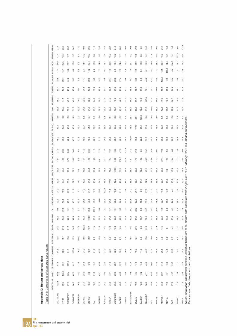
196ECBRisk measurement and systemic riskApril 2007
Ap
pen
dix
D:
Ret
urn
an
d s
pre
ad d
ata
Tab
le D
.3: C
orre
latio
ns o
f eur
o ar
ea b
ank
retu
rns
DE
UT
SC
HE
H
YP
OD
RE
SD
NE
RC
OM
ME
RZ
B
GB
ER
LIN
D
EP
FA
B
NP
PA
R
CA
S
GE
NE
R
NA
TE
XIS
INT
ES
A
UN
ICR
ED
IT
PA
OLO
CA
PIT
A
SA
NT
AN
DE
RB
ILB
AO
B
AN
ES
PIN
GA
BN
AM
RO
F
OR
TIS
A
LMA
NIJ
ALP
HA
BC
PS
AM
PO
IRB
AN
DE
UT
SC
HE
10
0.0
60.8
67.6
64.8
16.8
24.7
48.6
19.5
52.6
24.2
33.6
35.9
43.1
31.9
48.0
49.1
1 2.6
55.9
56.2
47.7
33.8
17.1
27.9
17.4
27.1
HY
PO
60.8
100.
056
.462
.014
.721
.040
.821
.843
.119
.933
.129
.940
.028
.839
.842
.310
.248
.547
.142
.028
.415
.125
.513
.923
.6
DR
ES
DN
ER
67.6
56.4
100.
061
.313
.621
.542
.919
.143
.622
.031
.928
.137
.325
.242
.443
.813
.650
.049
.643
.931
.015
.025
.717
.323
.5
CO
MM
ER
Z
64.8
62.0
61.3
100.
016
.324
.242
.421
.743
.721
.232
.732
.039
.830
.943
.545
.911
.951
.749
.645
.428
.514
.825
.815
.524
.5
BG
BE
RLI
N
16.8
14.7
13.6
16.3
100.
011
.611
.92.
712
.57.
19.
38.
98.
67.
813
.812
.13.
012
.010
.09.
47.
67.
49.
69.
313
.3
DE
PF
A
24.7
21.0
21.5
24.2
11.6
100.
019
.111
.421
.814
.313
.615
.816
.411
.019
.320
.75.
824
.322
.921
.817
.79.
114
.113
.219
.1
BN
PP
AR
48
.640
.842
.942
.411
.919
.110
0.0
25.0
66.1
31.1
34.8
37.4
42.8
33.9
49.8
51.0
16.7
54.2
52.8
46.3
29.9
14.2
25.4
19.0
30.3
CA
19
.521
.819
.121
.72.
711
.425
.010
0.0
25.0
12.3
15.4
10.4
19.3
11.3
20.2
22.2
5.3
28.2
24.7
26.0
15.9
4.8
10.3
6.0
11.8
SG
EN
ER
52
.643
.143
.643
.712
.521
.866
.125
.010
0.0
29.9
34.1
38.9
44.1
32.9
51.3
52.5
15.4
57.2
55.3
48.8
32.7
17.3
24.9
19.6
33.8
NA
TE
XIS
24.2
19.9
22.0
21.2
7.1
14.3
31.1
12.3
29.9
100.
016
.518
.521
.113
.424
.226
.49.
827
.127
.721
.715
.510
.716
.113
.418
.7
INT
ES
A
33.6
33.1
31.9
32.7
9.3
13.6
34.8
15.4
34.1
16.5
100.
046
.549
.348
.136
.338
.111
.139
.637
.936
.823
.711
.920
.515
.322
.1
UN
ICR
ED
IT
35.9
29.9
28.1
32.0
8.9
15.8
37.4
10.4
38.9
18.5
46.5
100.
050
.548
.335
.739
.512
.340
.140
.634
.623
.69.
018
.413
.621
.9
PA
OLO
43.1
40.0
37.3
39.8
8.6
16.4
42.8
19.3
44.1
21.1
49.3
50.5
100.
047
.646
.147
.912
.248
.648
.541
.327
.412
.324
.417
.326
.0
CA
PIT
A
31.9
28.8
25.2
30.9
7.8
11.0
33.9
11.3
32.9
13.4
48.1
48.3
47.6
100.
034
.336
.69.
534
.633
.330
.719
.65.
616
.213
.920
.8
SA
NT
AN
DE
R48
.039
.842
.443
.513
.819
.349
.820
.251
.324
.236
.335
.746
.134
.310
0.0
76.8
22.3
55.1
55.7
46.6
30.3
17.0
29.7
18.9
30.8
BIL
BA
O
49.1
42.3
43.8
45.9
12.1
20.7
51.0
22.2
52.5
26.4
38.1
39.5
47.9
36.6
76.8
100.
021
.156
.056
.448
.932
.918
.031
.018
.530
.6
BA
NE
SP
12.6
10.2
13.6
11.9
3.0
5.8
16.7
5.3
15.4
9.8
11.1
12.3
12.2
9.5
22.3
21.1
100.
012
.513
.011
.06.
45.
110
.85.
89.
0
AB
NA
MR
O
56.2
47.1
49.6
49.6
10.0
22.9
52.8
24.7
55.3
27.7
37.9
40.6
48.5
33.3
55.7
56.4
13.0
73.7
100.
059
.140
.018
.128
.519
.133
.6
ING
55
.948
.550
.051
.712
.024
.354
.228
.257
.227
.139
.640
.148
.634
.655
.156
.012
.510
0.0
73.7
65.1
42.3
18.7
29.9
21.7
35.7
FO
RT
IS
47.7
42.0
43.9
45.4
9.4
21.8
46.3
26.0
48.8
21.7
36.8
34.6
41.3
30.7
46.6
48.9
11.0
65.1
59.1
100.
045
.017
.324
.319
.130
.0
ALM
AN
IJ33
.828
.431
.028
.57.
617
.729
.915
.932
.715
.523
.723
.627
.419
.630
.332
.96.
442
.340
.045
.010
0.0
12.5
20.4
15.9
23.7
ALP
HA
17.1
15.1
15.0
14.8
7.4
9.1
14.2
4.8
17.3
10.7
11.9
9.0
12.3
5.6
17.0
18.0
5.1
18.7
18.1
17.3
12.5
100.
014
.413
.113
.9
BC
P27
.925
.525
.725
.89.
614
.125
.410
.324
.916
.120
.518
.424
.416
.229
.731
.010
.829
.928
.524
.320
.414
.410
0.0
13.1
19.2
SA
MP
O17
.413
.917
.315
.59.
313
.219
.06.
019
.613
.415
.313
.617
.313
.918
.918
.55.
821
.719
.119
.115
.913
.113
.110
0.0
20.4
IRB
AN
27.1
23.6
23.5
24.5
13.3
19.1
30.3
11.8
33.8
18.7
22.1
21.9
26.0
20.8
30.8
30.6
9.0
35.7
33.6
30.0
23.7
13.9
19.2
20.4
100.
0
Dat
a so
urce
: Dat
astr
eam
and
ow
n ca
lcul
atio
ns.
Not
es: C
orre
latio
n co
e ffic
ient
s be
twee
n in
divi
dual
ban
ks a
re in
%. R
etur
n da
ta s
erie
s ru
n fr
om 2
Apr
il 19
92 to
27
Feb
ruar
y 20
04. n
.a. m
eans
not
ava
ilabl
e.

197ECB
Risk measurement and systemic riskApril 2007
Ap
pen
dix
D:
Ret
urn
an
d s
pre
ad d
ata
Tab
le D
.4: C
orre
latio
ns o
f US
ban
k re
turn
s
CIT
IGJP
MO
RG
AN
WA
CH
OV
IAF
AR
GO
B
ON
EW
AS
HIN
GF
LEE
T
BN
YO
RK
S
ST
RE
ET
NT
RU
ST
M
ELL
ON
B
CO
RP
C
ITY
CO
PN
C
KE
YC
OS
UT
RU
ST
CO
ME
RIC
A
UN
ION
BA
NK
AM
SO
UT
HH
UN
TIN
G
BB
T
53B
AN
CO
SO
TR
US
T
RE
GIO
NS
BA
ME
RIC
A
CIT
IG10
0.0
64.8
55.9
51.7
52.6
38.1
55.7
55.8
51.6
50.6
55.0
41.2
53.0
54.4
53.2
56.5
51.7
33.5
46.1
41.1
50.0
47.0
45.0
44.3
61.0
JP M
OR
GA
N64
.810
0.0
59.2
54.6
56.7
39.3
60.9
61.2
52.7
52.1
60.7
43.4
56.4
58.1
56.8
58.2
55.6
33.7
47.9
44.4
50.3
47.5
46.1
48.6
64.7
WA
CH
OV
IA55
.959
.210
0.0
56.6
60.2
40.5
60.0
56.9
50.0
51.8
58.6
48.6
61.2
61.6
61.9
64.5
59.2
38.4
51.3
48.5
55.0
51.7
48.8
51.5
65.9
FA
RG
O
51.7
54.6
56.6
100.
053
.041
.555
.257
.450
.748
.856
.746
.258
.459
.658
.363
.055
.733
.648
.742
.952
.551
.149
.049
.660
.4
BO
NE
52.6
56.7
60.2
53.0
100.
040
.755
.255
.550
.249
.155
.645
.058
.259
.457
.561
.454
.835
.247
.444
.550
.048
.545
.849
.259
.7
WA
SH
ING
38.1
39.3
40.5
41.5
40.7
100.
039
.340
.739
.140
.641
.635
.143
.944
.245
.143
.942
.427
.437
.534
.141
.941
.741
.540
.341
.2
FLE
ET
55
.760
.960
.055
.255
.239
.310
0.0
59.6
51.4
52.8
60.5
48.9
60.6
60.4
59.0
62.6
59.6
36.8
52.2
46.7
53.8
51.0
49.0
52.3
59.3
BN
YO
RK
55
.861
.256
.957
.455
.540
.759
.610
0.0
58.0
59.1
63.4
49.2
58.4
61.6
59.5
63.7
59.7
35.7
50.6
46.9
54.5
52.2
47.9
51.8
60.1
SS
TR
EE
T51
.652
.750
.050
.750
.239
.151
.458
.010
0.0
59.8
58.1
45.3
51.4
53.5
50.6
56.2
51.8
33.9
46.6
43.8
46.3
49.5
44.4
47.2
52.4
NT
RU
ST
50
.652
.151
.848
.849
.140
.652
.859
.159
.810
0.0
55.3
48.4
51.7
54.9
52.7
54.4
53.1
37.2
48.2
46.6
50.0
51.9
46.9
49.8
49.9
ME
LLO
N
55.0
60.7
58.6
56.7
55.6
41.6
60.5
63.4
58.1
55.3
100.
048
.659
.162
.960
.563
.557
.737
.051
.545
.153
.850
.150
.752
.960
.5
BC
OR
P
41.2
43.4
48.6
46.2
45.0
35.1
48.9
49.2
45.3
48.4
48.6
100.
049
.951
.049
.550
.348
.833
.445
.644
.048
.743
.145
.346
.546
.2
CIT
YC
O53
.056
.461
.258
.458
.243
.960
.658
.451
.451
.759
.149
.910
0.0
62.3
63.0
65.9
60.6
36.9
54.6
49.0
54.1
53.1
52.7
54.4
61.3
PN
C
54.4
58.1
61.6
59.6
59.4
44.2
60.4
61.6
53.5
54.9
62.9
51.0
62.3
100.
064
.066
.262
.236
.752
.747
.855
.753
.252
.353
.862
.0
KE
YC
O53
.256
.861
.958
.357
.545
.159
.059
.550
.652
.760
.549
.563
.064
.010
0.0
66.2
63.1
37.4
52.7
51.1
57.1
53.9
53.4
55.9
59.3
SU
TR
US
T56
.558
.264
.563
.061
.443
.962
.663
.756
.254
.463
.550
.365
.966
.266
.210
0.0
64.1
40.0
55.6
48.9
56.9
55.5
53.7
57.2
64.7
CO
ME
RIC
A
51.7
55.6
59.2
55.7
54.8
42.4
59.6
59.7
51.8
53.1
57.7
48.8
60.6
62.2
63.1
64.1
100.
037
.753
.750
.055
.954
.151
.455
.658
.6
UN
ION
BA
NK
33.5
33.7
38.4
33.6
35.2
27.4
36.8
35.7
33.9
37.2
37.0
33.4
36.9
36.7
37.4
40.0
37.7
100.
037
.231
.835
.631
.736
.635
.238
.4
AM
SO
UT
H
46.1
47.9
51.3
48.7
47.4
37.5
52.2
50.6
46.6
48.2
51.5
45.6
54.6
52.7
52.7
55.6
53.7
37.2
100.
046
.151
.145
.548
.952
.050
.3
HU
NT
ING
41
.144
.448
.542
.944
.534
.146
.746
.943
.846
.645
.144
.049
.047
.851
.148
.950
.031
.846
.110
0.0
49.2
46.7
48.0
47.8
46.2
BB
T
50.0
50.3
55.0
52.5
50.0
41.9
53.8
54.5
46.3
50.0
53.8
48.7
54.1
55.7
57.1
56.9
55.9
35.6
51.1
49.2
100.
052
.551
.752
.052
.5
53B
AN
CO
47.0
47.5
51.7
51.1
48.5
41.7
51.0
52.2
49.5
51.9
50.1
43.1
53.1
53.2
53.9
55.5
54.1
31.7
45.5
46.7
52.5
100.
049
.449
.548
.8
SO
TR
US
T
45.0
46.1
48.8
49.0
45.8
41.5
49.0
47.9
44.4
46.9
50.7
45.3
52.7
52.3
53.4
53.7
51.4
36.6
48.9
48.0
51.7
49.4
100.
052
.049
.4
RE
GIO
NS
44.3
48.6
51.5
49.6
49.2
40.3
52.3
51.8
47.2
49.8
52.9
46.5
54.4
53.8
55.9
57.2
55.6
35.2
52.0
47.8
52.0
49.5
52.0
100.
051
.2
BA
ME
RIC
A61
.064
.765
.960
.459
.741
.259
.360
.152
.449
.960
.546
.261
.362
.059
.364
.758
.638
.450
.346
.252
.548
.849
.451
.210
0.0
Dat
a so
urce
: Dat
astr
eam
and
ow
n ca
lcul
atio
ns.
Not
es: C
orre
latio
n co
effic
ient
s be
twee
n in
divi
dual
ban
ks a
re in
%. R
etur
n da
ta s
erie
s ru
n fr
om 2
Apr
il 19
92 to
27
Feb
ruar
y 20
04. n
.a. m
eans
not
ava
ilabl
e.

198ECBRisk measurement and systemic riskApril 2007
Appendix E. Results for GARCH-filtered data
A widely recognized feature of nancial market returns is volatility
clustering (see, e.g., Bollerslev, Chou and Kroner, 1992). So, a ques-
tion that comes to mind is to which extent the extreme dependence
between bank stock returns and its changes we discover in this paper
is associated with changes in volatility. In this appendix we therefore
reproduce the results of the paper for return data that are ltered of
conditional heteroskedasticity.
Before providing some answers to this question, we need to rst
establish the relationship between the ltered data and the objectives of
our paper. The main objective of our work is to measure systemic risk
in banking on the basis of market data. The amount of systemic risk
in banking is instrumental for the assessment of nancial stability and
for the design of policies to preserve the stability of nancial systems,
such as banking regulation and crisis management.
The indicators of banking system stability we are using are designed
to satisfy the demand by policy makers who need to have a view about
the likelihood of crises and who need to devise the best nancial regula-
tions to preserve nancial stability. To assess system stability banking
supervisors need to know how likely it is that one or several banks
break down given that other banks break down or how likely it is
that one or several banks break down given that there is an adverse
macroeconomic shock. They are not interested in two-sided volatility
of bank stock returns per se or in its persistence. In addition, bank-
ing regulations are determined in advance for longer periods of time.
They cannot be changed within a few days. So, they need to be based
on long-term structural risk assessments and not on the likelihood of
volatility tomorrow given today’s volatility. This is why for the ques-
tions we are interested in straight returns are preferable to volatility of
returns and unconditional modelling is preferable to conditional mod-
els. In contrast, conditional models will be preferable for short-term
volatility forecasting, as today’s volatility is informative for tomorrow’s
volatility. This type of analysis maybe more important for short-term
pricing of nancial instruments.
Although the indicators (2.1) and (2.2) are the right ones for answer-
ing the questions of interest in this paper, we may learn from unclus-
tered return data more about the statistical components of spillover and
extreme systematic risk in banking. For example, Poon et al. (2004)
argue that conditional heteroskedasticity is an important source of ex-
treme dependence in stock markets in general, but not the only one.

199ECB
Risk measurement and systemic riskApril 2007
So, in this appendix we ask to which extent the extreme dependence
of bank stock returns uncovered above results from univariate volatil-
ity clustering or multivariate dependence in volatilities. The next sub-
section reports the multivariate spillover probabilities (2.1) for unclus-
tered return data and the subsequent one the tail- estimations (2.2).
The lter used in both cases is a standard GARCH(1,1) process.
E.1. Bank contagion risk. Tables E.1 through E.5 reproduce tables
3, 4, 5, 9 and 10 in the main text for GARCH- ltered returns. While
extreme dependence generally tends to decrease, the qualitative results
are quite similar to the ones for plain bank returns. Only very few
of the spillover risk changes in Europe (table 9) seem to be entirely
related to volatility clustering. But clustering plays more of a role
in the di erences between domestic and cross-border spillovers (table
4). Multivariate spillover risk in the US and Europe, as well as its
changes over time seem little related to volatility clustering (tables 5
and 10). This is also con rmed by the dotted lines in gures 1 and 2,
which describe the same stastics as the solid lines for GARCH- ltered
returns.
E.2. Aggregate banking system risk. Tables E.6 through E.10 re-
produce tables 6, 7, 8, 11 and 12 in the main text for unclustered
returns. As for the spillover risk above, dependencies generally de-
crease, but none of the qualitative results is fundamentally changed.
Again this is also con rmed by the dotted lines in gure 3, which illus-
trate the more muted changes in GARCH- ltered tail- s and the same
direction of their movements.
Overall, we can conclude that in line with the results of Poon et al.
(2004) for stock markets in general, part of the extreme dependencies
in bank stock returns we nd in this paper are related to time-varying
volatility and volatility clustering. From the little exercise in this ap-
pendix we can not ascertain whether this phenomenon is related to
the marginal distributions or to multivariate dependence of volatilities.
Nevertheless, the primary results that supervisors should pay atten-
tion to in order to assess general banking system stability and decide
upon regulatory policies are the unadjusted spillover and systematic
risk probabilities.

200ECBRisk measurement and systemic riskApril 2007
Table E.1. Domestic versus cross-border extreme spilloverrisk among euro area banks for GARCH- ltered data: Esti-
mations
Largest bank 1 2 3 4 5
Conditioning banks: German
Germany 12.3 63.7 70.7 57.0 35.0
Netherlands 5.1 23.3 35.9 6.3 19.4
France 1.6 20.7 32.1 9.4 10.3
Spain 1.8 12.1 14.4 8.9 31.0
Italy 1.5 3.7 6.6 1.2 5.5
Belgium 3.1 18.0 18.7 6.5 4.2
Ireland 1.9 4.2 7.4 7.4 19.8
Portugal 1.4 6.7 11.2 5.6 8.3
Finland 0.6 2.5 5.4 1.0 3.3
Greece 0.7 0.9 2.5 0.2 0.8
Conditioning banks: French
France 1.4 30.2 6.6
Germany 0.4 15.0 3.0
Netherlands 1.6 14.8 7.7
Italy 0.7 5.3 1.7
Spain 1.3 23.4 5.2
Belgium 0.9 12.0 4.3
Ireland 0.8 3.2 3.0
Portugal 1.0 4.9 10.1
Finland 0.1 0.6 1.5
Greece 0.2 0.7 0.3
Conditioning banks: Italian
Italy 3.2 13.4 18.9
Germany 2.4 8.8 7.6
Netherlands 1.5 10.2 8.2
Spain 1.1 9.1 3.7
France 1.2 6.6 2.4
Belgium 1.1 5.5 2.5
Ireland 1.1 2.3 3.6
Portugal 0.5 1.1 1.9
Finland 0.4 1.4 1.5
Greece 1.6E-0.2 0.3 0.6
Conditioning banks: Spanish
Spain 21.6 13.5
Germany 3.8 3.0
Netherlands 6.4 6.8
France 7.0 7.8
Italy 0.8 1.9
Belgium 3.6 1.5
Ireland 2.7 1.9
Portugal 1.4 0.6
Finland 0.3 0.5
Greece 0.5 0.4
Note: The table shows the same results as table 3 in the main text for data that have been ltered for volatility
clustering. The returns used here are the residuals of a GARCH(1,1) process tted on the original excess returns.
The table reports estimated extreme spillover probabilities between banks, as de ned in (2.1). Each column
shows the spillover probabilities for the largest bank of the country mentioned on the left-hand side conditional
on a set of banks from either the same country or other countries. The number of conditioning banks varies
from 1 to 5 for Germany (top panel), 1 to 3 for France (upper middle panel), 1 to 3 for Italy (lower middle panel)
and 1 to 2 for Spain (bottom panel). For example, the 2 column contains probabilities for a stock market crash
of the largest bank in each country, conditional on crashes of the 2nd and 3rd largest bank in Germany, France,
Italy or Spain. All probabilities are estimated with the extension of the approach by Ledford and Tawn (1996)
described in section 3 and reported in %. Univariate crash probabilities (crisis levels) are set to = 0 05%.

201ECB
Risk measurement and systemic riskApril 2007
Table E.2. Domestic versus cross-border extreme spilloverrisk among euro area banks for GARCH- ltered data: Tests
Largest bank 1 2 3 4 5
Conditioning banks: German
Netherlands 1.49 1.56 0.84 0.81 0.11
France ***3.30 1.23 0.30 0.51 1.06
Spain ***2.93 **2.11 -0.18 -0.28 0.29
Italy ***2.82 ***3.75 -0.35 -0.13 -0.50
Belgium **2.07 1.55 0.46 -0.26 -0.76
Ireland **2.47 ***3.34 -1.54 1.20 0.91
Portugal ***3.06 ***3.71 0.46 1.31 0.29
Finland ***4.21 ***2.67 -1.55 -0.10 -0.83
Greece ***3.59 ***4.12 ***-3.15 -1.31 -0.61
Conditioning banks: French
Germany **2.02 -0.49 0.85
Netherlands -0.25 1.25 1.37
Spain 0.07 -0.84 0.22
Italy 0.84 -1.53 -0.03
Belgium 0.63 0.84 1.28
Ireland 0.58 ***-3.34 -1.39
Portugal 0.36 -1.50 1.13
Finland ***2.91 ***-4.22 **-2.21
Greece **2.29 ***-3.76 ***-2.77
Conditioning banks: Italian
Germany 0.26 0.28 -0.09
Netherlands 1.18 1.06 0.21
Spain 1.51 -0.59 -0.27
France 1.32 0.28 -0.09
Belgium 1.25 -0.52 -0.72
Ireland 1.07 -0.75 -1.00
Portugal **2.01 -0.65 -1.42
Finland **2.54 -0.90 -1.47
Greece ***3.36 -1.86 **-2.20
Conditioning banks: Spanish
Germany ***2.88 -0.69
Netherlands **2.17 -0.30
France *1.82 -0.05
Italy ***4.35 -0.57
Belgium ***2.84 -0.62
Ireland ***2.82 -0.91
Portugal ***4.03 -0.77
Finland ***5.55 -1.05
Greece ***4.47 -1.29
Note: The table shows the same results as table 4 in the main text for data that have been ltered for volatility
clustering. The returns used here are the residuals of a GARCH(1,1) process tted on the original excess
returns. The table reports the statistics for the cross sectional test (4.5). Within each panel the degree of
extreme domestic spillover risk is compared with the degree of extreme cross-border spillover risk for a given
xed number of conditioning banks. So, each T-statistic describes whether the di erences between domestic and
cross-border values of that entered the estimations in table 3 are statistically signi cant. For example, in the
top panel the test statistic in the row "Netherlands" and the column 1 indicates whether the di erence between
the for the spillover probability between ABN AMRO and HypoVereinsbank and the between Deutsche
Bank and HypoVereinsbank is statistically signifcant. The null hypothesis is that the respective two s are
equal. Insigni cant T-statistics imply that the domestic and cross-border spillover risks are indistinguishable.
A signi cant rejection with positive sign implies that cross-border spillover risk is statistically smaller than its
domestic counterpart; and a rejection with negative sign implies that cross-border risk is larger than domestic
risk. The critical values of the test are 1.65, 1.96 and 2.58 for the 10%, 5% and 1% levels, respectively. Asterisks
*, ** and *** indicate rejections of the null hypothesis at 10%, 5% and 1% signi cance.
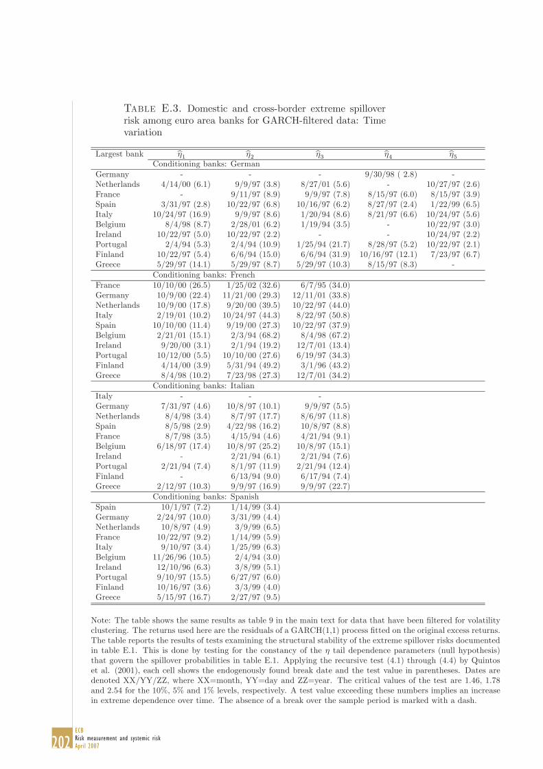
202ECBRisk measurement and systemic riskApril 2007
Table E.3. Domestic and cross-border extreme spilloverrisk among euro area banks for GARCH- ltered data: Time
variation
Largest bank 1 2 3 4 5
Conditioning banks: German
Germany - - - 9/30/98 ( 2.8) -
Netherlands 4/14/00 (6.1) 9/9/97 (3.8) 8/27/01 (5.6) - 10/27/97 (2.6)
France - 9/11/97 (8.9) 9/9/97 (7.8) 8/15/97 (6.0) 8/15/97 (3.9)
Spain 3/31/97 (2.8) 10/22/97 (6.8) 10/16/97 (6.2) 8/27/97 (2.4) 1/22/99 (6.5)
Italy 10/24/97 (16.9) 9/9/97 (8.6) 1/20/94 (8.6) 8/21/97 (6.6) 10/24/97 (5.6)
Belgium 8/4/98 (8.7) 2/28/01 (6.2) 1/19/94 (3.5) - 10/22/97 (3.0)
Ireland 10/22/97 (5.0) 10/22/97 (2.2) - - 10/24/97 (2.2)
Portugal 2/4/94 (5.3) 2/4/94 (10.9) 1/25/94 (21.7) 8/28/97 (5.2) 10/22/97 (2.1)
Finland 10/22/97 (5.4) 6/6/94 (15.0) 6/6/94 (31.9) 10/16/97 (12.1) 7/23/97 (6.7)
Greece 5/29/97 (14.1) 5/29/97 (8.7) 5/29/97 (10.3) 8/15/97 (8.3) -
Conditioning banks: French
France 10/10/00 (26.5) 1/25/02 (32.6) 6/7/95 (34.0)
Germany 10/9/00 (22.4) 11/21/00 (29.3) 12/11/01 (33.8)
Netherlands 10/9/00 (17.8) 9/20/00 (39.5) 10/22/97 (44.0)
Italy 2/19/01 (10.2) 10/24/97 (44.3) 8/22/97 (50.8)
Spain 10/10/00 (11.4) 9/19/00 (27.3) 10/22/97 (37.9)
Belgium 2/21/01 (15.1) 2/3/94 (68.2) 8/4/98 (67.2)
Ireland 9/20/00 (3.1) 2/1/94 (19.2) 12/7/01 (13.4)
Portugal 10/12/00 (5.5) 10/10/00 (27.6) 6/19/97 (34.3)
Finland 4/14/00 (3.9) 5/31/94 (49.2) 3/1/96 (43.2)
Greece 8/4/98 (10.2) 7/23/98 (27.3) 12/7/01 (34.2)
Conditioning banks: Italian
Italy - - -
Germany 7/31/97 (4.6) 10/8/97 (10.1) 9/9/97 (5.5)
Netherlands 8/4/98 (3.4) 8/7/97 (17.7) 8/6/97 (11.8)
Spain 8/5/98 (2.9) 4/22/98 (16.2) 10/8/97 (8.8)
France 8/7/98 (3.5) 4/15/94 (4.6) 4/21/94 (9.1)
Belgium 6/18/97 (17.4) 10/8/97 (25.2) 10/8/97 (15.1)
Ireland - 2/21/94 (6.1) 2/21/94 (7.6)
Portugal 2/21/94 (7.4) 8/1/97 (11.9) 2/21/94 (12.4)
Finland - 6/13/94 (9.0) 6/17/94 (7.4)
Greece 2/12/97 (10.3) 9/9/97 (16.9) 9/9/97 (22.7)
Conditioning banks: Spanish
Spain 10/1/97 (7.2) 1/14/99 (3.4)
Germany 2/24/97 (10.0) 3/31/99 (4.4)
Netherlands 10/8/97 (4.9) 3/9/99 (6.5)
France 10/22/97 (9.2) 1/14/99 (5.9)
Italy 9/10/97 (3.4) 1/25/99 (6.3)
Belgium 11/26/96 (10.5) 2/4/94 (3.0)
Ireland 12/10/96 (6.3) 3/8/99 (5.1)
Portugal 9/10/97 (15.5) 6/27/97 (6.0)
Finland 10/16/97 (3.6) 3/3/99 (4.0)
Greece 5/15/97 (16.7) 2/27/97 (9.5)
Note: The table shows the same results as table 9 in the main text for data that have been ltered for volatility
clustering. The returns used here are the residuals of a GARCH(1,1) process tted on the original excess returns.
The table reports the results of tests examining the structural stability of the extreme spillover risks documented
in table E.1. This is done by testing for the constancy of the tail dependence parameters (null hypothesis)
that govern the spillover probabilities in table E.1. Applying the recursive test (4.1) through (4.4) by Quintos
et al. (2001), each cell shows the endogenously found break date and the test value in parentheses. Dates are
denoted XX/YY/ZZ, where XX=month, YY=day and ZZ=year. The critical values of the test are 1.46, 1.78
and 2.54 for the 10%, 5% and 1% levels, respectively. A test value exceeding these numbers implies an increase
in extreme dependence over time. The absence of a break over the sample period is marked with a dash.
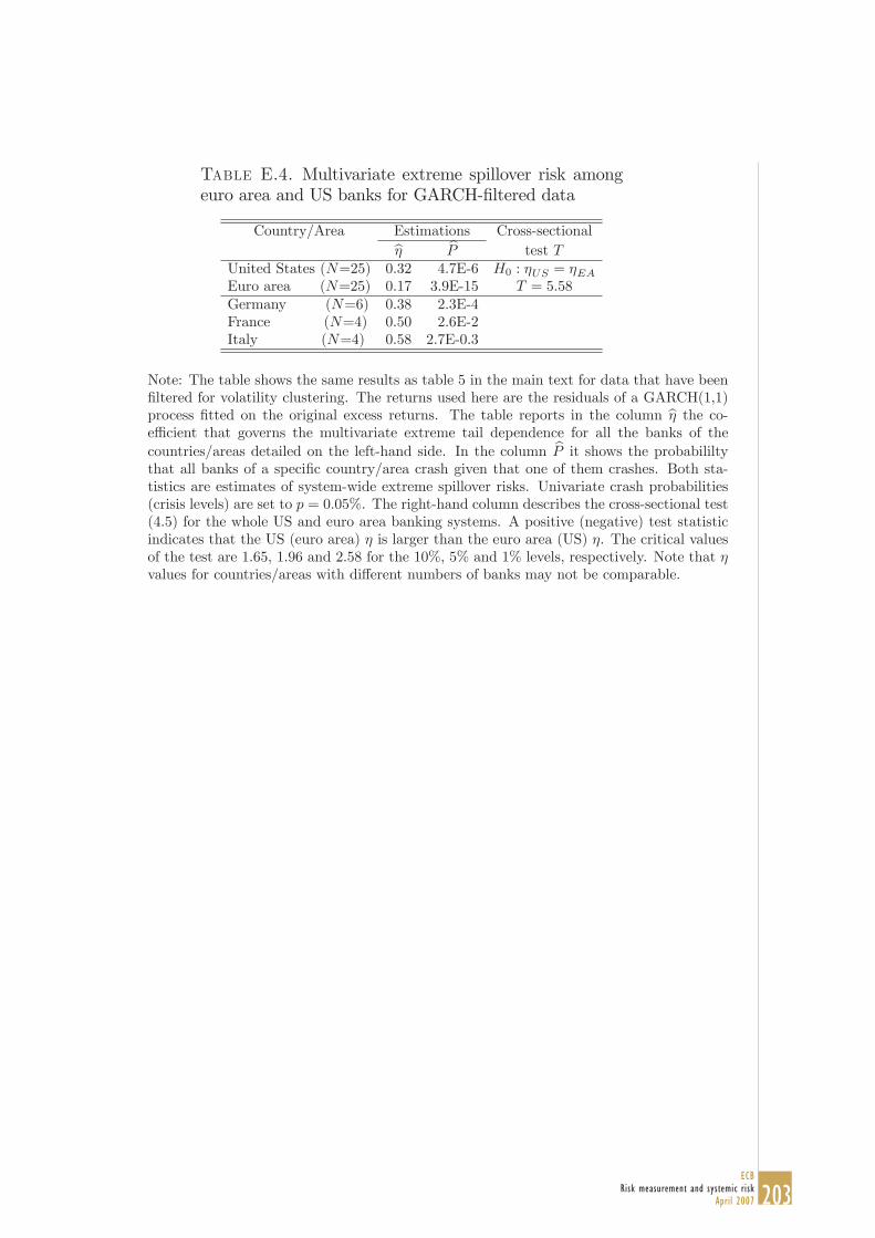
203ECB
Risk measurement and systemic riskApril 2007
Table E.4. Multivariate extreme spillover risk amongeuro area and US banks for GARCH- ltered data
Country/Area Estimations Cross-sectional
b
b test
United States ( =25) 0.32 4.7E-6 0 : =Euro area ( =25) 0.17 3.9E-15 = 5 58Germany ( =6) 0.38 2.3E-4
France ( =4) 0.50 2.6E-2
Italy ( =4) 0.58 2.7E-0.3
Note: The table shows the same results as table 5 in the main text for data that have been
ltered for volatility clustering. The returns used here are the residuals of a GARCH(1,1)
process tted on the original excess returns. The table reports in the column b the co-
e cient that governs the multivariate extreme tail dependence for all the banks of the
countries/areas detailed on the left-hand side. In the column b it shows the probabililty
that all banks of a speci c country/area crash given that one of them crashes. Both sta-
tistics are estimates of system-wide extreme spillover risks. Univariate crash probabilities
(crisis levels) are set to = 0 05%. The right-hand column describes the cross-sectional test(4.5) for the whole US and euro area banking systems. A positive (negative) test statistic
indicates that the US (euro area) is larger than the euro area (US) . The critical values
of the test are 1.65, 1.96 and 2.58 for the 10%, 5% and 1% levels, respectively. Note that
values for countries/areas with di erent numbers of banks may not be comparable.

204ECBRisk measurement and systemic riskApril 2007
Table E.5. Multivariate extreme spillover risk amongeuro area and US banks for GARCH- ltered data: Time
variation
Country/Area Full sample Second sub-sample break tests
break test Endogenous Exogenous
United States ( =25) 11/13/95 (4.8) - n.a.
Euro area ( =25) 12/5/96 (4.9) (B) 1/18/99 (5.3) (1.5)
Germany ( =6) - - (1.6)
- -
France ( =4) 6/7/95 (19.1) 11/27/01 (23.7) (-2.8)
(B) 3/4/97 (4.6) (B) 8/25/00 (3.8)
Italy ( =4) - - (1.4)
Note: The table shows the same results as table 10 in the main text for data that have been
ltered for volatility clustering. The returns used here are the residuals of a GARCH(1,1)
process tted on the original excess returns. The table reports tests and estimations assess-
ing time variation in the multivariate spillover probabilities of table E.4. The column on
the left displays estimated break dates and values from the recursive Quintos et al. (2001)
test (4.1) through (4.4) applied to the parameter governing the extreme tail dependence
of the banks located in the countries/areas displayed on the extreme left. Dates are denoted
XX/YY/ZZ, where XX=month, YY=day and ZZ=year. The forward recursive version of
the test is used, unless marked otherwise. (B) marks the backward recursive version of the
test. The critical values of the test are 1.46, 1.78 and 2.54 for the 10%, 5% and 1% levels,
respectively. The middle columns show pre- and post-break estimates for . The columns
on the right display two tests that assess the occurrence of further breaks in the second half
of the sample. The rst one is the same as the one on the left-hand side. The second one is a
simple di erences-in-means test based on (4.5). The exogenous break point is chosen to be
1/1/99, the time of the introduction of the euro. Critical values for this test are 1.65, 1.96
and 2.58 for the 10%, 5% and 1% signi cance levels. Note that values for countries/areas
with di erent numbers of banks may not be comparable.

205ECB
Risk measurement and systemic riskApril 2007
Table E.6. Extreme systematic risk (tail- s) of euroarea banks for GARCH- ltered data
Bank Aggregate risk factor
Bank index Stock index Global bank Global stock Yield spread
DEUTSCHE 34.3 19.1 8.1 4.2 9.0E-6
HYPO 12.7 6.9 1.7 1.2 3.0E-2
DRESDNER 20.1 17.3 7.1 3.7 7.7E-3
COMMERZ 14.8 11.0 3.0 1.9 6.9E-2
BGBERLIN 2.0 1.4 0.6 0.4 7.3E-2
DEPFA 2.1 2.1 0.7 0.9 6.2E-2
BNPPAR 12.7 8.5 5.3 3.6 3.9E-2
CA 2.2 1.4 0.4 0.6 0.2
SGENERAL 19.3 11.8 5.8 4.2 4.8E-2
NATEXIS 0.8 1.0 1.5 0.7 3.5E-2
INTESA 4.6 3.5 1.7 1.9 1.7E-0.2
UNICREDIT 4.3 3.7 3.6 2.2 6.8E-2
PAOLO 10.7 10.8 4.3 2.9 6.0E-2
CAPITA 6.1 5.5 2.3 2.6 0.1
SANTANDER 9.8 10.9 4.5 3.4 7.0E-2
BILBAO 16.0 11.6 6.0 5.3 7.0E-2
BANESP 1.5 0.9 0.6 0.3 2.0E-3
ING 22.7 23.4 8.5 4.2 8.5E-2
ABNAMRO 14.3 12.3 6.7 3.6 4.5E-2
FORTIS 17.2 10.1 4.9 2.7 2.2E-2
ALMANIJ 2.7 3.1 1.8 1.0 8.5E-2
ALPHA 1.9 2.5 0.9 0.6 2.2E-2
BCP 4.0 3.2 2.3 1.3 0.1
SAMPO 1.6 1.9 0.6 0.5 3.8E-2
IRBAN 6.3 6.5 2.0 1.7 1.8E-2
average 9.8 7.6 3.4 2.2 6.5E-2
st. dev. 8.5 6.1 2.5 1.5 4.4E-2
Note: The table shows the same results as table 6 in the main text for data that have been
ltered for volatility clustering. The returns used here are the residuals of a GARCH(1,1)
process tted on the original excess returns. The table exhibits the estimates of extreme
systematic risk (2.2) (tail- s) for individual euro area banks and for the euro area banking
system as a whole. The entries show the probability that a given bank crashes given that
a market indicator of aggregate risk crashes (or in the case of the yield spread booms).
Results are reported for ve di erent aggregate risk factors: The euro area banking sector
sub-index, the euro area stock index, the world banking sector sub-index, the world stock
index and the euro area high-yield bond spread. Data for the euro area yield spread are
only available from 1998 to 2004. All probabilities are estimated with the extension of the
approach by Ledford and Tawn (1996) described in section 3 and reported in %. Univariate
crash probabilities (crisis levels) are set to = 0 05%. The average and the standard
deviation at the bottom of the table are calculated over the 25 individual tail- s in the
upper rows, respectively.

206ECBRisk measurement and systemic riskApril 2007
Table E.7. Extreme systematic risk (tail- s) of USbanks for GARCH- ltered data
Bank Aggregate risk factor
Bank index Stock index Global bank Global stock Yield spread
CITIG 32.6 24.8 6.3 11.7 6.9E-2
JPMORGAN 24.9 9.0 3.3 4.9 0.1
BOA 28.2 12.4 5.9 7.2 0.2
WACHO 25.2 10.5 4.1 5.2 0.2
FARGO 14.6 7.5 4.5 6.5 4.1E-2
BONEC 27.1 12.6 3.6 6.0 0.1
WASHMU 9.8 4.5 2.3 2.4 0.1
FLEET 15.2 13.9 5.4 6.4 0.2
BNYORK 17.5 9.5 4.9 7.1 0.1
STATEST 16.0 14.3 7.2 10.3 0.4
NOTRUST 14.6 9.9 4.2 5.6 0.2
MELLON 25.0 19.6 5.7 10.2 0.3
USBANC 10.9 3.8 3.5 2.4 6.4E-2
CITYCO 24.9 11.8 4.7 7.0 9.9E-2
PNC 14.6 10.4 5.3 6.9 0.1
KEYCO 23.6 11.0 2.3 4.9 8.8E-2
SUNTRUST 19.7 15.4 5.7 8.9 0.2
COMERICA 24.3 14.0 4.7 7.3 0.2
UNIONBAN 5.9 2.7 2.3 2.8 0.1
AMSOUTH 10.5 6.5 6.6 4.5 0.2
HUNTING 10.4 5.5 4.3 3.3 0.1
BBT 9.8 5.0 4.1 4.2 0.1
53BANCO 11.2 5.9 2.0 2.5 9.7E-2
SOTRUST 12.6 4.3 3.0 2.6 0.1
RFCORP 11.4 9.5 3.8 4.5 0.2
average 17.6 78.4 4.4 5.8 0.1
st. dev. 7.3 4.7 1.4 2.6 7.1E-2
Note: The table shows the same results as table 7 in the main text for data that have been
ltered for volatility clustering. The returns used here are the residuals of a GARCH(1,1)
process tted on the original excess returns. The table exhibits the estimates of extreme
systematic risk (2.2) (tail- s) for individual US banks and for the US banking system as
a whole. The entries show the probability that a given bank crashes given that a market
indicator of aggregate risk crashes (or in the case of the yield spread booms). Results are
reported for ve di erent aggregate risk factors: The US banking sector sub-index, the
US stock index, the world banking sector sub-index, the world stock index and the US
high-yield bond spread. All probabilities are estimated with the extension of the approach
by Ledford and Tawn (1996) described in section 3 and reported in %. Univariate crash
probabilities (crisis levels) are set to = 0 05%. The average and the standard deviationat the bottom of the table are calculated over the 25 individual tail- s in the upper rows,
respectively.

207ECB
Risk measurement and systemic riskApril 2007
Table E.8. Comparisons of extreme systematic riskacross di erent banking systems for GARCH- ltered
data
Aggregate risk factor
Banking system Bank index Stock index Global bank Global stock Yield spread
0.83 0.78 0.72 0.74 0.53
0.76 0.74 0.69 0.67 0.50
0.74 0.71 0.69 0.67 0.50
0.79 0.76 0.69 0.66 0.50
0.74 0.74 0.70 0.69 0.53
Null hypothesis
= **2.09 1.25 0.85 **2.28 0.71
= **2.25 **1.99 1.12 **2.35 0.72
= 0.91 0.56 1.16 ***2.72 0.87
= *1.92 1.14 0.54 1.60 0.19
Note: The table shows the same results as table 9 in the main text for data that have been
ltered for volatility clustering. The returns used here are the residuals of a GARCH(1,1)
process tted on the original excess returns. The table exhibits the average tail dependence
parameters that govern the tail- estimates reported in tables E.6 and E.7 for the US, euro
area, French, German and Italian banking system (upper panel) and the statistics of tests
examining di erences in extreme systematic risk between the US and euro area banking
systems (lower panel). Each is calculated as the mean of tail- dependence parameters
across all the banks in our sample for the respective country/area. The tests are applications
of the cross-sectional test (4.5). The null hypothesis is that extreme systematic risk in the
US banking system is the same as in the other banking systems. A positive (negative) test
statistic indicates that extreme systematic risk in the US banking system (in the respective
euro area banking system) is larger than in the respective euro area (US) banking system.
The critical values of the test are 1.65, 1.96 and 2.58 for the 10%, 5% and 1% levels,
respectively. All results are reported for the ve di erent aggregate risk factors: The euro
area/US banking sector sub-index, the euro area/US stock index, the world banking sector
sub-index, the world stock index and the euro area/US high-yield bond spread. Univariate
crash probabilities (crisis levels) are set to = 0 05%.
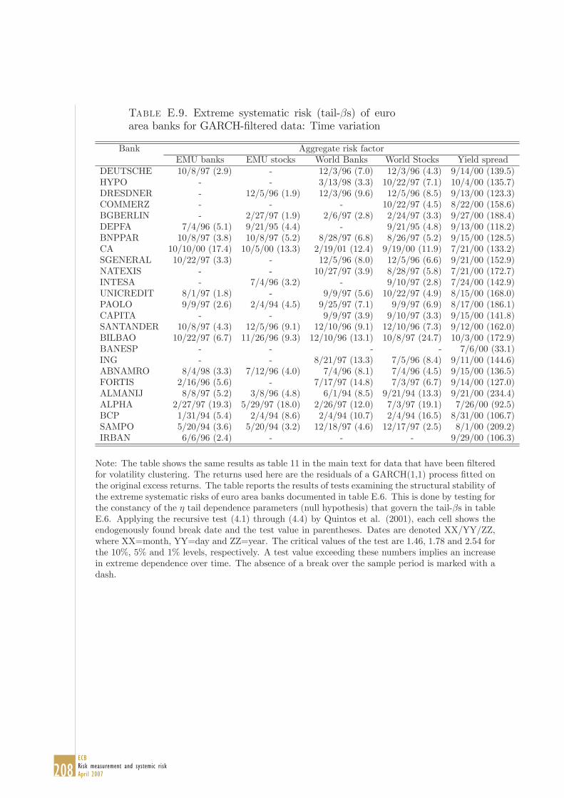
208ECBRisk measurement and systemic riskApril 2007
Table E.9. Extreme systematic risk (tail- s) of euroarea banks for GARCH- ltered data: Time variation
Bank Aggregate risk factor
EMU banks EMU stocks World Banks World Stocks Yield spread
DEUTSCHE 10/8/97 (2.9) - 12/3/96 (7.0) 12/3/96 (4.3) 9/14/00 (139.5)
HYPO - - 3/13/98 (3.3) 10/22/97 (7.1) 10/4/00 (135.7)
DRESDNER - 12/5/96 (1.9) 12/3/96 (9.6) 12/5/96 (8.5) 9/13/00 (123.3)
COMMERZ - - - 10/22/97 (4.5) 8/22/00 (158.6)
BGBERLIN - 2/27/97 (1.9) 2/6/97 (2.8) 2/24/97 (3.3) 9/27/00 (188.4)
DEPFA 7/4/96 (5.1) 9/21/95 (4.4) - 9/21/95 (4.8) 9/13/00 (118.2)
BNPPAR 10/8/97 (3.8) 10/8/97 (5.2) 8/28/97 (6.8) 8/26/97 (5.2) 9/15/00 (128.5)
CA 10/10/00 (17.4) 10/5/00 (13.3) 2/19/01 (12.4) 9/19/00 (11.9) 7/21/00 (133.2)
SGENERAL 10/22/97 (3.3) - 12/5/96 (8.0) 12/5/96 (6.6) 9/21/00 (152.9)
NATEXIS - - 10/27/97 (3.9) 8/28/97 (5.8) 7/21/00 (172.7)
INTESA - 7/4/96 (3.2) - 9/10/97 (2.8) 7/24/00 (142.9)
UNICREDIT 8/1/97 (1.8) - 9/9/97 (5.6) 10/22/97 (4.9) 8/15/00 (168.0)
PAOLO 9/9/97 (2.6) 2/4/94 (4.5) 9/25/97 (7.1) 9/9/97 (6.9) 8/17/00 (186.1)
CAPITA - - 9/9/97 (3.9) 9/10/97 (3.3) 9/15/00 (141.8)
SANTANDER 10/8/97 (4.3) 12/5/96 (9.1) 12/10/96 (9.1) 12/10/96 (7.3) 9/12/00 (162.0)
BILBAO 10/22/97 (6.7) 11/26/96 (9.3) 12/10/96 (13.1) 10/8/97 (24.7) 10/3/00 (172.9)
BANESP - - - - 7/6/00 (33.1)
ING - - 8/21/97 (13.3) 7/5/96 (8.4) 9/11/00 (144.6)
ABNAMRO 8/4/98 (3.3) 7/12/96 (4.0) 7/4/96 (8.1) 7/4/96 (4.5) 9/15/00 (136.5)
FORTIS 2/16/96 (5.6) - 7/17/97 (14.8) 7/3/97 (6.7) 9/14/00 (127.0)
ALMANIJ 8/8/97 (5.2) 3/8/96 (4.8) 6/1/94 (8.5) 9/21/94 (13.3) 9/21/00 (234.4)
ALPHA 2/27/97 (19.3) 5/29/97 (18.0) 2/26/97 (12.0) 7/3/97 (19.1) 7/26/00 (92.5)
BCP 1/31/94 (5.4) 2/4/94 (8.6) 2/4/94 (10.7) 2/4/94 (16.5) 8/31/00 (106.7)
SAMPO 5/20/94 (3.6) 5/20/94 (3.2) 12/18/97 (4.6) 12/17/97 (2.5) 8/1/00 (209.2)
IRBAN 6/6/96 (2.4) - - - 9/29/00 (106.3)
Note: The table shows the same results as table 11 in the main text for data that have been ltered
for volatility clustering. The returns used here are the residuals of a GARCH(1,1) process tted on
the original excess returns. The table reports the results of tests examining the structural stability of
the extreme systematic risks of euro area banks documented in table E.6. This is done by testing for
the constancy of the tail dependence parameters (null hypothesis) that govern the tail- s in table
E.6. Applying the recursive test (4.1) through (4.4) by Quintos et al. (2001), each cell shows the
endogenously found break date and the test value in parentheses. Dates are denoted XX/YY/ZZ,
where XX=month, YY=day and ZZ=year. The critical values of the test are 1.46, 1.78 and 2.54 for
the 10%, 5% and 1% levels, respectively. A test value exceeding these numbers implies an increase
in extreme dependence over time. The absence of a break over the sample period is marked with a
dash.

209ECB
Risk measurement and systemic riskApril 2007
Table E.10. Extreme systematic risk (tail- s) of USbanks for GARCH- ltered data: Time variation
Bank Aggregate risk factor
Bank index Stock index Global bank Global stock Yield spread
CITIG - - 7/4/96 (7.7) 11/18/94 (8.4) 10/24/00 (97.9)
JPMORGAN - - 2/19/96 (3.6) 1/8/96 (3.3) 10/16/00 (74.8)
BOA - 4/1/96 (5.4) 12/5/96 (13.6) 2/15/96 (11.8) 9/26/00 (65.7)
WACHO - - 9/16/94 (8.7) 12/4/95 (5.2) 10/16/00 (66.4)
FARGO 3/7/96 (2.9) - 9/21/95 (7.2) 1/8/96 (5.6) 9/28/00 (35.3)
BONEC 9/15/95 (2.2) 10/19/95 (3.8) 10/23/95 (7.1) 6/5/95 (9.0) 10/20/00 (78.8)
WASHMU 3/1/96 (1.8) 2/26/96 (2.2) 2/27/97 (10.8) 2/23/96 (7.2) 12/13/00 (57.6)
FLEET 12/6/95 (2.1) 3/12/97 (7.7) 10/7/97 (13.7) 1/9/96 (12.2) 10/5/00 (52.3)
BNYORK - 1/8/96 (1.9) 7/4/96 (10.6) 1/8/96 (13.9) 9/22/00 (49.5)
STATEST 12/15/95 (12.9) 12/15/95 (11.9) 9/29/95 (12.1) 9/15/95 (7.5) 10/11/00 (139.1)
NOTRUST 12/3/96 (6.1) 12/15/95 (4.2) 10/7/97 (3.3) 12/5/96 (5.7) 9/29/00 (60.3)
MELLON 9/15/95 (2.8) 10/19/95 (4.2) 9/9/97 (7.7) 11/18/94 (10.2) 10/16/00 (90.3)
USBANC 12/15/95 (5.4) 12/11/95 (2.1) 10/13/97 (9.2) 9/15/95 (8.0) 2/19/01 (58.3)
CITYCO 12/10/96 (2.4) 12/2/96 (4.7) 1/8/96 (9.6) 12/15/95 (11.4) 10/5/00 (37.7)
PNC 3/7/96 (2.2) 10/19/95 (5.5) 7/4/96 (18.8) 10/20/95 (14.5) 11/9/00 (39.4)
KEYCO - 10/24/95 (3.1) 6/19/96 (2.4) 10/24/95 (7.1) 1/1/01 (44.7)
SUNTRUST 10/6/95 (5.3) 12/4/95 (5.1) 10/24/95 (8.7) 10/24/95 (16.9) 12/5/00 (42.4)
COMERICA - 1/8/96 (2.3) 7/4/96 (7.0) 9/15/95 (10.2) 10/4/00 (61.1)
UNIONBAN 6/27/97 (6.3) 3/4/98 (5.4) 1/5/98 (2.9) 1/5/98 (6.5) 10/25/00 (32.3)
AMSOUTH 11/13/95 (3.4) 12/4/95 (4.3) 12/10/96 (7.7) 1/5/96 (4.4) 10/17/00 (54.5)
HUNTING 2/4/97 (5.9) 1/22/97 (8.2) 2/27/97 (9.1) 1/22/97 (9.3) 10/5/00 (50.5)
BBT 3/6/96 (4.7) 7/20/98 (7.2) 5/22/98 (14.0) 3/7/96 (8.1) 10/5/00 (35.5)
53BANCO 1/2/96 (2.3) 12/13/95 (1.3) 1/8/96 (9.1) 12/7/95 (3.9) 10/17/00 (44.5)
SOTRUST 2/26/97 (10.6) 6/17/96 (9.2) 7/4/96 (9.0) 3/7/96 (7.0) 11/21/00 (41.1)
RFCORP 3/7/96 (4.1) 2/23/96 (12.3) 12/5/96 (9.2) 2/23/96 (12.7) 9/20/00 (46.4)
Note: The table shows the same results as table 12 in the main text for data that have been ltered
for volatility clustering. The returns used here are the residuals of a GARCH(1,1) process tted on
the original excess returns. The table reports the results of tests examining the structural stability
of the extreme systematic risks of US banks documented in table E.7. This is done by testing for
the constancy of the tail dependence parameters (null hypothesis) that govern the tail- s in table
E.7. Applying the recursive test (4.1) through (4.4) by Quintos et al. (2001), each cell shows the
endogenously found break date and the test value in parentheses. Dates are denoted XX/YY/ZZ,
where XX=month, YY=day and ZZ=year. The critical values of the test are 1.46, 1.78 and 2.54 for
the 10%, 5% and 1% levels, respectively. A test value exceeding these numbers implies an increase
in extreme dependence over time. The absence of a break over the sample period is marked with a
dash.

210ECBRisk measurement and systemic riskApril 2007
AbstractUsing a unique dataset, this paper develops three distinct methods to quantify the risk of a sys-temic failure in the global banking system. We examine a sample of 334 banks (representing 80% of global bank equity) in 28 countries around 6 global financial crises (such as the Asian and Rus-sian crises and September 11, 2001), and show that these crises did not create large probabilities of global financial system failure. We show that cumulative negative abnormal returns for the subset of banks not directly exposed to a negative shock (unexposed banks) rarely exceed a few percent. More precise point estimates of the likelihood of systemic failure are obtained from structural models. These estimates suggest that systemic risk is limited even during major finan-cial crises. For example, maximum likelihood estimation of bank failure probabilities implied by equity prices suggests the Asian crisis induced less than a 1% increase in the probability of sys-temic failure. Also, we demonstrate that estimates of systemic risk can be obtained from default probabilities of banks that are implied in their equity option prices. The largest values are ob-tained for the Russian crisis and September 11 and these show increases in estimated average de-fault probabilities of only around 1-2%. The findings of low probabilities of a breakdown of the international financial system suggests that the distress of central bankers, regulators and politi-cians about such events may be overrated, and that existing policies and intervention methods are likely to be adequate for limiting systemic risk.
Keywords: Systemic risk, default risk, credit risk, banks, exposure, emerging markets, 9/11
JEL Classification: G3, F4, F3
* Lancaster University, Management School, Lancaster LA1 4YX, United Kingdom, Phone: +44 (1524) 592 083, Fax: +1 (425) 952 10 70, Email: <[email protected]>, Internet: <http://www.lancs.ac.uk/staff/bartras1/>
† Corresponding author. Kenan-Flagler Business School, University of North Carolina at Chapel Hill, CB 3490 McColl Building, Chapel Hill, NC 27599-3490, USA, Phone: +1 (919) 962-9250, Fax: +1 (919) 962-2068, Email: <[email protected]>, Internet: <http://intranet.kenan-flagler.unc.edu/faculty/browngr/>.
‡ McCombs School of Business, University of Texas at Austin, Austin, TX 78712, USA. Phone: +1 (512) 471-6587, Fax: +1 (512) 471-5073, Email: <[email protected]>.The authors gratefully acknowledge research funding by the Center for Financial Research of the FDIC, Lancaster University, Lancaster University Management School, the Leverhulme Trust, and The Bank of America Faculty Development Fund, as well as support by Global Reports, Perfect Information, Fitch Ratings and Thomson Fi-nancial in establishing the dataset. The authors also thank Robert Bliss, Hans Degryse, Jean Dermine, Eva Gutierrez, Philipp Hartmann, Shelagh Heffernan, Jean Helwege, Armen Hovakimian, Donald Morgan, Roberto Rigobon, Anthony Saunders, Lynn Shibut, Christian Upper and Giuseppe Vulpes as well as seminar participants at the FDIC Summer Research Workshop, the FIRS conference in Capri, the 2005 NBER conference on “Risks of Financial Institutions”, NBER's 2005 Universities Research Conference on “Structural Changes in the Global Economy: Implications for Monetary Policy and Financial Regulation”, the Fourth Joint Central Bank Research Conference on “Risk Measurement and Systemic Risk”, the 2005 American Finance Association Annual Meeting, the 2004 European Finance Association Annual Meeting, the 2004 Financial Management Association Annual Meeting, the 2005 Australasian Conference on Banking and Finance, the EMG/ESRC workshop on "Interna-tional Diversification and Contagion" at Cass Business School, The Bank of England, Darden School of Business, Lancaster University, Temple University, University of North Carolina, University of Texas at Austin, Vanderbilt University and Wake Forest University. Florian Bardong and Nishad Kapadia provided excellent research assis-tance.
ESTIMATING SYSTEMIC RISK IN THE INTERNATIONAL FINANCIAL SYSTEM
SÖHNKE M. BARTRAM*, GREGORY W. BROWN†, AND JOHN E. HUND‡

211ECB
Risk measurement and systemic riskApril 2007
“In practice, the policy choice of how much, if any, extreme market risk should be absorbed by government authorities is fraught with many complexities. Yet we central bankers make this decision every day, either explic-itly, or implicitly through inadvertence. Moreover, we can never know for sure whether the decisions we make are appropriate. The question is not whether our actions are seen to have been necessary in retrospect; the absence of a fire does not mean that we should not have paid for fire insurance. Rather, the question is whether, ex ante, the probability of a systemic collapse was sufficient to warrant intervention. Often, we cannot wait to see whether, in hindsight, the problem will be judged to have been an isolated event and largely benign.”
International Financial Risk Management, Re-marks by Chairman Alan Greenspan before the Council on Foreign Relations, Washington, D.C. November 19, 2002
Systemic risk in the banking system has rightly attracted the attention of financial researchers (as
well as regulators and policymakers) literally since the genesis of the discipline; bank failure and
either simultaneous or subsequent macroeconomic collapse represents a financial dislocation with
large and far-reaching consequences. Recently, dramatic increases in capital mobility, relaxations
in international lending restrictions, and changes in capital allocation rules have raised the spectre
that credit and currency crises in emerging markets might bleed into developed credit markets via
disruptions in local lending channels. Others have argued that recent financial innovations (the
burgeoning credit derivatives market for instance) and the increased activity of non-banking fi-
nancial intermediaries (re-insurance companies, for example) may have lessened the risk that sys-
temic shocks are transmitted throughout the global banking system. Indeed, much of the argu-
ment over Basel II credit allocation rules has focused upon the ability of large financial institu-
tions to internally measure and manage the risk of credit crises without transmitting such shocks
to other banks.
Using unique data on exposure measures, this paper directly tests the strength of the
transmission mechanism between banks under the assumption of capital (equity) market effi-
ciency for a large sample of international banks; in essence, it uses systematic risk to test for sys-
temic risk. Specifically, we examine a sample of banks around significant emerging market cur-
rency and credit crises and show that there are no abnormal returns to banks without exposure to
the crises, whereas exposed banks tend to have abnormal returns over the crisis period. Fur-
thermore, using a modified version of the Merton structural model of the firm, we extract the
default probabilities associated with both exposed and unexposed banks both pre- and post-crisis
and show that there are no “flow-through” effects of the crisis on a bank’s probability of failure,
conditional on its exposure level. Lastly, we demonstrate the feasibility of an approach using op-
tion data and equity prices to infer systemic probabilities of bank failure. The implication here is

212ECBRisk measurement and systemic riskApril 2007
that using three separate approaches to infer the increased risk of systemic banking failure pro-
vides little evidence of systemic transmission of financial shocks through developed economies
even prior to the imposition of Basel II capital rules.
Financial economists in academia, central banks and international organizations alike have
intensely studied various facets of the recent financial crises in Latin America, Asia and Russia.
While theoretical models, e.g. by Freixas, Parigi and Rochet (2000), Allen and Gale (1998), and
Rochet and Triole (1996), analyze systemic risk in interbank lending relationships, nearly all of the
empirical work focuses indeed not on systemic risk per se, but on contagion effects in order to
identify the mechanics and channels through which these crises spread across markets and coun-
tries.1 To illustrate, Kho, Lee and Stulz (2000) study the effect of currency crises and the LTCM
crisis on a sample of 78 U.S. banks and document that banks with exposures to a crisis country
are adversely affected by crisis events and positively by IMF bailout announcements. Similarly,
Kho and Stulz (2000) examine the impact of the Asian crisis on bank indices in four developed
and six Asian countries. Bae, Karolyi and Stulz (2003) study the probability of joint occurrences
of extreme returns across countries (co-exceedances) and find that contagion depends on interest
rates, exchange rate changes, and conditional volatility, and that the United States are not im-
mune from contagion from Latin America, but are insulated from Asian contagion. Linkages be-
tween economies in crisis periods and potential spillover effects from one country to another
may, for instance, exist in the form of trade (Glick and Rose, 1999; Van Rijckeghem and Weder,
2001), or through financial linkages (Baig and Goldfajn, 1999; Goldfajn and Valdés, 1998). In
contrast, the analysis in this paper pertains directly to the phenomenon of systemic risk and at-
tempts to provide an empirical assessment of the likelihood of a failure of the global banking sys-
tem. It thus addresses the important issue of quantifying the consequences of contagious effects,
rather than explaining their existence.
Conceptually, a systemic failure in the global banking system could be defined as a failure
(seizing) of the global inter-bank payment system or a loss of confidence in banks which results
in a global ‘bank-run’. For example, payment failures could mean that banks not receiving pay-
ments on loans (explicit or implicit) would become technically insolvent. Cascading bank insol-
vencies and bank-runs could cause additional financial and economic spillovers such as rapid
1 Karolyi (2003) gives an excellent analysis and critique of different approaches to define and measure contagion. De Bandt and Hartmann (2000) offer a broad review of the theoretical and empirical literature on contagion and its systemic implications.

213ECB
Risk measurement and systemic riskApril 2007
credit reduction, and ultimately, macroeconomic contraction (see, for example, Bernanke (1983)).
Prior research has discussed how different types of shocks might cause systemic risk. For exam-
ple, Kaufman (2000) describes systemic risks that can arise from a “big shock” (e.g., failure of a
major bank ), “spillovers” (e.g., East Asian contagion), and “common shock” (e.g., 9/11). Other
researchers have distinguished between credit and operational risks. Since there does not exist an
easy or accepted way of classifying shocks by type (and we examine only a few events), we do not
attempt to draw conclusions about how different types of shocks affect changes in systemic risk
probabilities.
Our first method for estimating this risk of a systemic failure relies on measuring the im-
pact of global financial shocks on the stock price of a subset of banks that are not directly ex-
posed to the shock. Specifically, the abnormal performance of these stocks should reflect primar-
ily the probability of systemic failure in the banking system. In efficient capital markets, negative
information such as devaluations of emerging market currencies or the tragedy of 9/11 will affect
bank stock prices only if banks are exposed to the particular events. In contrast, unexposed bank
stock prices should be largely unaffected by these events. As a result, stock market reactions of
unexposed banks to crisis events can be interpreted as a crude measure of systemic risk. This is
because negative returns of these banks are not due to direct exposure to the crises per se, but they
are the result of negative returns of exposed banks that affect unexposed banks through the fi-
nancial system.2 Our analysis is based primarily on a sample of 334 banks in 28 countries repre-
senting about 80% of global bank equity. The first of our three approaches examines equity re-
turns of unexposed banks during financial crises. Both raw returns and cumulative abnormal re-
turns (CARs) for unexposed banks show relatively small declines (typically less than 4%) regard-
less of time horizon or exposure definition. The exception is immediately after 9/11 when CARs
for unexposed banks are in the range of -4% to -6%.
We also provide more precise point estimates of the likelihood of systemic failure based
on stock return and options data. With regard to stock return data, we use structural credit risk
models such as Merton (1974) and Leland and Toft (1996) to derive maximum likelihood esti-
mates of default for the sample banks. In particular, we can estimate the default probability of a
bank as a function of its characteristics such as market value, face value of debt, expected return,
2 Even in the absence of systemic failure, financial crises could on average have a negative effect on global econo-mies and therefore on banks in general. If we measure this effect, it will bias our estimates of systemic risk upward.

214ECBRisk measurement and systemic riskApril 2007
etc. While the models rely on several simplifications, model misspecification may largely wash out
in intertemporal comparisons of the recovered default probabilities. Consequently, we interpret
the difference between average pre-crisis and intra-crisis probabilities as a measure of systemic
failure. Our results suggest very little chance of increased systemic failure during any of the crises,
although there is a noticeable reaction to the LTCM credit crisis in the aftermath of the Russian
shock. For example, the largest increase in average default probabilities for unexposed banks oc-
curs during the Asian crisis when probabilities increase from 2.1% to 2.8%. Our estimates of in-
creases in systemic failure are less than 1% across all crises, with much of the impact on unex-
posed banks generated by European banks.
Our third approach for assessing systemic risk in the banking system comes from estimat-
ing bank default probabilities implied by equity option prices. This method has the advantage of
not relying on relatively infrequent (and stale) accounting data. In addition, the model can be es-
timated real-time using exclusively live market quotations thus making it a potentially valuable
regulatory tool. Our analysis assumes a particular model for option prices that explicitly includes
the probability of bankruptcy. Parameters of the model are estimated using a large set of publicly
traded options on a subset of European and U.S. banks. The model makes the important as-
sumption that over a finite horizon stocks follow a delta-geometric random walk (see Câmara
(2004)) and thus have a finite chance of going bankrupt. The valuation equations can be inverted
to yield the probability of bankruptcy. Because of data limitations, the sample is restricted to 14
European and 62 U.S. banks. Again, we study the difference in implied default probabilities be-
tween exposed and unexposed banks and find that none of the crises are associated with a sub-
stantial increase in systemic risk. The crises events with the largest impacts are the Rus-
sian/LTCM crisis and 9/11, but these events engender an average increase of only about 2% in
the default probability for the unexposed banks.
The results in this paper have important policy implications. While a priori a justifiable and
sensible concern, the findings of low probabilities of a meltdown of the international financial
system suggest that the distress of central bankers, regulators and politicians about such events
may be disproportionate. In essence, this would be empirical confirmation of the simulation evi-
dence presented by Gould, Koury, and Naftilan (2004). Of course, the lack of systemic risk may
also be a result of contemporaneous and judicious policy actions by central bankers and regula-
tors. Thus, the findings could be interpreted as justifying the responses of these actors during the
crises. Either way, given that chances of systemic failure appear low even during major financial

215ECB
Risk measurement and systemic riskApril 2007
crises, it seems that financial intermediaries on a global scale are more efficient and robust than
often thought (or feared), and that current policy tools and responses may be more than suffi-
cient.

216ECBRisk measurement and systemic riskApril 2007
References
Acharya, V. 2001. Theory of Systemic Risk and Design of Prudential Bank Regulation. London Business School working paper.
Allen, F., and D. Gale 1998. Optimal Financial Crises. Journal of Finance 53:4: 1245-1284.
Angelini, P., G. Maresca, and D. Russo 1996. Systemic risk in the netting system. Journal of Banking and Finance 20:5: 853-868.
Bae, K.-H., G.A. Karolyi, and R.M. Stulz 2003. A new approach to measuring financial conta-gion. Review of Financial Studies, forthcoming.
Baig, T., and I. Goldfajn 1999. Financial market contagion in the Asian crisis, IMF staff papers 46:2: 167-195.
Bandt, O. de, and P. Hartmann 2000. Systemic risk: A survey. European Central Bank Working Paper No. 35.
Bernanke, B., 1983. Non-monetary effects of the financial crisis in the propagation of the Great Depression. American Economic Review 73, 257–263.
Bessler, W., and T. Nohel 2000. Asymmetric information, dividend reductions, and contagion effects in bank stock returns. Journal of Banking and Finance 24:11: 1831-1849.
Bongini, P., L. Laeven, and G. Majnoni, 2002, How good is the market at assessing bank fragility? A horse race between different factors. Journal of Banking and Finance 26, 1011-1028.
Breeden, D.T., and R.H. Litzenberger 1978. Prices of state-contingent claims implicit in option prices. Journal of Business 51:4: 621-651.
Burnside, C., M. Eichenbaum, and S. Rebelo 2001. Hedging and financial fragility in fixed ex-change rate regimes. European Economic Review 45:7: 1151-1193.
Câmara, A. 2004. A simple model for recovering implied bankruptcy probability from stock and option market prices. University of Michigan-Flint Working Paper.
Crosbie, P.J., and J.R. Bohn 2001. Modeling default risk. KMV: San Francisco.
Crouhy, M., D. Galai, and R. Mark 2000. A comparative analysis of current credit risk models. Journal of Banking and Finance 24: 59-117.
Darby, Michael 1994. Over-the-counter derivatives and systemic risk to the global financial sys-tem. NBER Working Paper Series, No. 4801.
Davis, P. 1995. Debt, financial fragility and systemic risk. Oxford University Press: Oxford.
Demirguc-Kunt, A. and E. Kane 2002. Deposit insurance around the globe: Where does it work? Journal of Economic Perspectives 16: 175-195.
DeNicolo, G., and M. Kwast. 2001. Systemic Risk and Financial Consolidation: Are They Re-lated? International Monetary Fund working paper.
Duan, J-C. 1994. Maximum likelihood estimation using price data of the derivative contract. Mathematical Finance 4: 155-167.
Duan, J-C. 2000. Correction: Maximum likelihood estimation using price data of the derivative contract. Mathematical Finance 10: 461-462.

217ECB
Risk measurement and systemic riskApril 2007
Duan, J-C., G. Gauthier, J.-G. Simonato, and S. Zaanoun 2003. Maximum likelihood estimation of structural credit spread models – deterministic and stochastic interest rates. University of Toronto Working Paper.
Duffie, D. and K. Wang 2004. Multi-period corporate failure prediction with stochastic covari-ates. Stanford University Working Paper.
Eisenbeis, R.A. 1997a. International settlements: A new source of systemic risk? Economic Re-view 82:2: 44-50.
Eisenbeis, R.A. 1997b. Bank deposits and credit as sources of systemic risk. Economic Review 82:3: 4-19.
Eisenberg, L. and Noe, T. 2001. Systematic Risk in Financial Systems. Management Science 47:236.
Ericsson, J., and J. Reneby 2004. Estimating structural bond pricing models. Journal of Business, forthcoming.
Fischer, Stanley 1999. Reforming the International Financial System. The Economic Journal 109: 557-576.
Freixas, X., B.M. Parigi, and J.-C. Rochet 2000. Systemic risk, interbank relations, and liquidity provision by the central bank. Journal of Money, Credit and Banking 32:3: 611-638.
Furfine, C. 2003. Interbank exposures: Quantifying the risk of contagion. Journal of Money, Credit and Banking 35:1: 111-129.
Glick. R., and A.K. Rose 1999. Contagion and trade: Why are currency crises regional? Journal of International Money and Finance 18:4: 603-.
Goldfajn, I., and R.O. Valdés 1998. Are currency crises predictable? European Economic Review 42:3-5: 873.
Gould, S., S.A. Khoury, and S.J. Naftilan, 2004, Systemic Risk : Simulating Local Shocks To A Global System, Claremont Colleges working paper.
Huang, J.-Z., and M. Huang 2003. How much of the corporate-Treasury yield spread is due to credit risk? Results from a new calibration approach. Stanford University Working Paper.
Jones, E.P., S.P. Mason and E. Rosenfeld 1984. Contingent claims analysis of corporate capital structures: An empirical investigation. Journal of Finance 49: 611-627.
Kaplan-Appio, I. 2002. Estimating the value of implicit government guarantees to Thai banks. Review of International Economics 10: 26-35.
Kaminsky, G. and C. Reinhart 1999. The Twin Crises: the causes of banking and balance-of-payments problems. American Economic Review 89: 473-500.
Karolyi, G.A. 2003. Does International Finance Contagion Really Exist. International Finance 6:2: 179-199.
Kaufman, G.G. 1994. Bank contagion: A review of theory and evidence. Journal of Financial Ser-vices Research 8:2: 123-150.
Kaufman, G.G. 2000. Banking and currency crises and systemic risk: A taxonomy and review. Financial Markets, Institutions and Instruments 9:2, 69-131.
Kaufman, G.G., and K.E. Scott 2003. What is systemic risk, and do bank regulators retard or contribute to it? Independent Review 7:3: 371-391.

218ECBRisk measurement and systemic riskApril 2007
Kho, B.-C., and R.M. Stulz 2000. Banks, the IMF, and the Asian crisis. Pacific-Basin Finance Journal 8: 177-216.
Kho, B.-C., D. Lee, and R.M. Stulz 2000. U.S. banks, crises, and bailouts: From Mexico to LTCM, American Economic Review 90:2: 28-31.
Krainer, J., and J.A. Lopez. 2001. Incorporating Equity Market Information into Supervisory Monitoring Models. FRBSF Working Paper 01-14.
Laeven, L. 2002. Bank Risk and Deposit Insurance. World Bank Economic Review 16: 109-137.
Leland, H.E. 2002. Predictions of expected default frequencies in structural models of debt. Uni-versity of California Working Paper.
Leland, H.E., and K.B. Toft 1996. Optimal capital structure, endogenous bankruptcy, and the term structure of credit spreads. Journal of Finance 51:3: 987-1019.
Marshall, D. 1998. Understanding the Asian crisis: Systemic risk as coordination failure. Eco-nomic Perspectives 22:3: 13-29.
Merton, R.C. 1977. An Analytic Derivation of the Cost of Deposit Insurance and Loan Guaran-tees. Journal of Banking and Finance 1: 3-11.
Merton, R.C. 1974. On the pricing of corporate debt: The risk structure of interest rates. Journal of Finance 28: 449-470.
Pettway, R., and J. Sinkey, 1980, Establishing on-site bank examination priorities: An early-warning system using accounting and market information. Journal of Finance 35:1, 137-150.
Rigshaw, G. 2001. Profits of Doom. Sunday Telegraph (London, U.K.), September 23, 2001.
Rochet, J., and J. Tirole 1996. Interbank lending and systemic risk. Journal of Money, Credit and Banking 28:4: 733-762.
Rogoff, K. 1999. International institutions for reducing global financial instability. Journal of Economic Perspectives 13:4: 21-42.
Ronn, E., and A. Verma 1986. Pricing risk-adjusted deposit insurance: An option-based model. Journal of Finance 41: 871-895.
Sanford, C. 1994. Financial markets in 2020. Economic Review. Federal Reserve Bank of Kansas City 79:1: 19-28.
Stiglitz, J. 1999. Reforming the global economic architecture: Lessons from recent crisis. Journal of Finance 54: 1508-1522.
Summers, L. 2000. International Financial Crises: Causes, Prevention, and Cures. American Eco-nomic Review 90: 1-15.
Swidler, S. and J.A. Wilcox 2002. Information about Bank Risk in Options Prices. Journal of Banking and Finance 26: 1033–1057.
Van Rijckeghem, C., and B. Weder 2001. Sources of contagion: Is it finance or trade? Journal of International Economics 54:2: 293-308.
Vassalou, M., and Y. Xing 2004. Default risk and equity returns. Journal of Finance 59:2: 831-68.

219ECB
Risk measurement and systemic riskApril 2007
Abstract
This paper studies the implications of the presence of a large speculator like George
Soros during a contagious currency crisis. The model shows that the presence of the
large speculator makes countries more vulnerable to crises, but mitigates contagion
of crises across countries. The model presents policy implications as to financial dis-
closure and size regulation of speculators such as hedge funds. First, financial disclo-
sure by speculators eliminates contagion, but may make countries more vulnerable to
crises. Second, regulating the size of speculators (e.g., prohibiting hedge funds from
high-leverage and thereby limiting the amount of short-selling) makes countries less
vulnerable to crises, but makes contagion more severe.
JEL classifications: F31; E58; D82; C72
Keywords: Contagion; Currency Crises; Global Game
∗E-mail: [email protected]†The author is deeply grateful to Steven N. Durlauf for his invaluable advice and constant encourage-
ment. The author also thanks Yeon-Koo Che, Charles Engel, Bruce Hansen, Graciela L. Kaminsky, BobStaiger and the stuff of the Bank of Japan for helpful suggestions. All possible remaining errors are mine.The views expressed in this paper are those of the author and do not necessarily reflect the official viewsof the Bank of Japan or IMES.
A LARGE SPECULATOR IN CONTAGIOUS CURRENCY CRISES: A SINGLE “GEORGE SOROS” MAKES COUNTRIES MORE VULNERABLE TO CRISES, BUT MITIGATES CONTAGION
KENSHI TAKETA*†

220ECBRisk measurement and systemic riskApril 2007
“Has anyone noticed just how small a player the IMF really is? That $18
billion U.S. contribution to the IMF, which has finally been agreed upon after
countless Administration appeals and conservative denunciations, is about the
same as the short position that [George] Soros single-handedly took against
the British pound in 1992 — and little more than half the position Soros’
Quantum Fund, Julian Robertson’s Tiger Fund, and a few others took against
Hong Kong last August [in 1997].”
— Paul Krugman, Soros’ Plea: Stop Me!1
1 Summary
This paper studies the implications of the presence of a large speculator like George Soros
during a contagious currency crisis.
The names of recent financial crises, such as the Mexican Tequila crises in 1994, the
Asian Flu in 1997, the Russian Virus in 1998, and the Brazilian Sneeze in 1999, suggest a
common feature. Clearly the common feature is “contagion,” where a financial crisis begins
locally, in some region, country, or institution, and subsequently spreads elsewhere. The
international transmission of financial shocks per se is not always a surprising phenomenon.
What is quite surprising in recent contagion episodes, however, is that the financial crises
in small economies like Thailand or Russia have devastating effects on economies of very
different sizes and structures, thousands of miles apart, with few direct trade or financial
links, and in very severe and unexpected ways.2 Put another way, it is quite surprising that
severe contagion of crises has happened across seemingly “unrelated” countries, originating
from crises in small economies. Why did Australian and South African stock market indices
fall by 14% in the turmoil over the Asian Flu?3 Why did the Brazilian stock market fall
by over 50% and the sovereign spreads of Brazil rise sharply during the Russian Virus?4
1See Krugman (1998).2Regarding the Russian Virus, Calvo, Izquierdo, and Talvi (2003) argue that “it was hard to even
imagine, ex ante, that a crisis in a country that represents less than 1 percent of world output would havesuch devastating effect on the world capital market.” (p.4)
3See Forbes (2004).4See Forbes and Rigobon (2001).

221ECB
Risk measurement and systemic riskApril 2007
While several contagion channels have been proposed in the literature, none seem able to
explain entirely the extent of contagion. This paper provides a complement to the growing
literature by extending the model presented in Taketa (2004).
Closely related to the issue of contagion, is the issue of “large” speculators. Large
speculators, like George Soros or Julian Robertson, have not only been blamed for desta-
bilizing the market unnecessarily during the turmoil of contagious currency crises, but
also for triggering these contagious crises by themselves. For instance, during the tur-
moil of the Asian Flu, the then prime minister of Malaysia, Mahathir Mohamad, accused
George Soros and others of being “the anarchists, self-serving rogues and international
brigandage”.5 There are two main reasons that these large speculators are often blamed.
First, they are considered to be able to affect the whole market to some degree. As op-
posed to small traders, they can exercise a disproportionate influence on the likelihood and
severity of a financial crisis by fermenting and orchestrating attacks against weakened cur-
rency pegs, as the opening quote of this paper suggests. Second, their personal funds are
often registered in so-called tax havens, typically small islands in the Caribbean, Europe,
and Asia Pacific. These “offshore” funds typically do not forward financial information
about themselves to other tax and financial authorities, since regulation in the tax havens
is often less stringent than that of major industrialized countries. Therefore, they are
often thought of as “monsters” whose true nature is unknown. Regardless of whether this
is factually correct, it is quite important to investigate how such speculators can affect the
market during contagious currency crises.
Following recent financial crises, the issue of contagion and that of large speculators
have been arguably the most serious concerns for policy makers in international finance.
Recent international policy discussions have revolved around questions on how to stop,
mitigate, or prevent contagion of financial crises in the presence of George Soros-like
speculators. In order to answer these questions, it is important to clarify two things: the
possible channels for contagion, and the influence of large speculators on the spread of
financial crises.
This paper attempts to answer these questions. To my knowledge, this work is the first5Financial Times, July 25, 1997.

222ECBRisk measurement and systemic riskApril 2007
to investigate in a unified framework the issue of contagion across unrelated countries and
that of a large speculator. By investigating these issues together, it becomes clear that
the presence of the large speculator, who typically does not disclose financial information
about himself to the regulatory authorities or to the market, has important implications
during a contagious currency crisis. The large speculator’s financial information (i.e., his
“type”) is private information. However, under some special situations such as financial
crises, this private information is revealed to the market to a limited degree. This revealed
information about his “type” can change the optimal behavior of other speculators who
did not know the information before the crisis, which in turn can cause contagion of crises
across unrelated countries.
The main findings of this paper are summarized as follows.
First, a single large speculator (“George Soros”) mitigates contagion compared with
small speculators, because he makes other small speculators more aggressive in attacking
the currency peg. This seems paradoxical, but can be explained as follows. I model conta-
gion using Bayesian updating to portray each speculator’s belief about other speculators’
types. When other speculators’ behavior differs greatly, the change in behavior due to
Bayesian updating becomes quite large, which in turn makes the contagion more severe.
Because one “George Soros” makes other small speculators more aggressive in attacking
the currency peg, speculators’ behavior converges even when their types are different. This
means that Bayesian updating in each speculator’s belief about other speculators’ types
does not matter much. Even when a speculator can distinguish between different types of
speculators, it is inconsequential since speculators of different types behave in a similarly
aggressive way due to the presence of a single “George Soros.”
Second, if the regulatory authorities can have large speculators such as George Soros
disclose their financial information, they can eliminate contagion but may make countries
more vulnerable to crises. This follows immediately from point two above. If small specu-
lators know the exact type of Soros from the beginning due to financial disclosure, there is
no room for Bayesian updating in belief about Soros’ type. No Bayesian updating means
no contagion in my model. However, if small speculators initially know that Soros is truly
223ECB
Risk measurement and systemic riskApril 2007
the most aggressive type, they can mimic this aggression by attacking the currency peg,
which makes countries more vulnerable to crises.
Third, if the regulatory authorities can limit the size of speculators by regulating the
amount of short-selling, they can make countries less vulnerable to crises but may make
contagion more severe. This is a mirror image of the finding that one large “George Soros”
makes countries more vulnerable to crises, but mitigates contagion.
2 Future Research
In some cases it is challenging to estimate the theoretical models due to data constraint.
In this section I argue that experimental analysis would be able to provide some useful
information to accompany the literature.
Corsetti, Dasgupta, Morris, and Shin (2004) show theoretically that the presence of
a large speculator causes all the remaining speculators to be more aggressive than the
case where there is no large speculator, as small speculators attack the currency when
fundamentals are stronger. Meanwhile, empirical evidence on the role of large speculators
is mixed.6 One reason for the mixed empirical results might be due to data constraint.
Their personal funds are typically registered in the so-called tax havens and they do not
have to disclose data as regulations in tax havens are far less stringent. As a result, it
is hard to obtain sufficiently detailed data to decisively determine the role of the large
speculator in financial crises.
trolled environment that “allows observations to be unambiguously interpreted in relation-
ship to the theory.” They report the results of experiments designed to test the predictions
of Corsetti, Dasgupta, Morris, and Shin (2004). In particular, the experiments test (a)
whether speculators are more likely to attack the peg when the economic fundamentals
are weaker, and (b) whether the large speculator makes small speculators more aggressive6See Brown, Goetzmann, and Park (1998), Fung and Hsieh (2000), Fung, Hsieh, and Tsatsaronis (2000),
and Corsetti, Pesenti, and Roubini (2002) among others.
Taketa, Suzuki-Löffelholz and Arikawa (2007) complement the literature by using
experimental analysis. As Roth (1995) argued, an experimental approach gives us a con-

224ECBRisk measurement and systemic riskApril 2007
in attacking the peg. Moreover, the experiments also test (c) whether the effect of the
recognition that “Soros appears” is symmetric to the effect of the recognition that “Soros
disappears” even though Corsetti, Dasgupta, Morris, and Shin (2004) do not deal with
this issue. This investigation would provide some possible clues to construct a dynamic
theoretical model in the future. The results of the experiments not only support the pre-
dictions of Corsetti, Dasgupta, Morris, and Shin (2004) but also suggest that the effect
of “Soros appears” is not symmetric to the effect of “Soros disappears”. Therefore, the
results indicate how we could extend the model of Corsetti, Dasgupta, Morris, and Shin
(2004) to explain the asymmetric effect.
For future research, I am planning to conduct experiments to test related theoretical
papers. Bannier (2005) highlights the role that the market sentiment has on the impact of
a large trader on a currency crisis. Corsetti, Guimaraes, and Roubini (2005) investigate
the role of the official creditor (the IMF or an international lender of last resort) as a
large player in the world economy. It is very likely that it is challenging to estimate these
models due to data constraint. Experimental analysis would be useful to complement the
literature.
225ECB
Risk measurement and systemic riskApril 2007
References
Bannier, C. E. (2005): “Big Elephants in Small Ponds: Do Large Traders Make Financial
Markets More Agrressive?,” Journal of Monetary Economics, 52(8), 1517–1531.
Brown, S. J., W. N. Goetzmann, and J. Park (1998): “Hedge Funds and the Asian
Currency Crisis of 1997,” NBER Working Paper 6427.
Calvo, G. A., A. Izquierdo, and E. Talvi (2003): “Sudden Stops, the Real Exchange
Rate, and Fiscal Sustainability: Argentina’s Lessons,” NBER Working Paper 9828.
Corsetti, G., A. Dasgupta, S. Morris, and H. S. Shin (2004): “Does One Soros
Make a Difference? A Theory of Currency Crises with Large and Small Traders,” Review
of Economic Studies, 71(1), 87–113.
Corsetti, G., B. Guimaraes, and N. Roubini (2005): “International Lending of Last
Resort and Moral Hazard: A Model of IMF’s Catalytic Finance,” Journal of Monetary
Economics, forthcoming.
Corsetti, G., P. Pesenti, and N. Roubini (2002): “The Role of Large Players in Cur-
rency Crises,” in Preventing Currency Crises in Emerging Markets, ed. by S. Edwards,
and J. A. Frankel. The University of Chicago Press.
Forbes, K. J. (2004): “The Asian Flu and Russian Virus: The International Transmis-
sion of Crises in Firm-Level Data,” Journal of International Economics, 63(1), 59–92.
Forbes, K. J., and R. Rigobon (2001): “Contagion in Latin America: Definitions,
Measurement, and Policy Implications,” Economia, 1(2), 1–46.
Fung, W., and D. A. Hsieh (2000): “Measuring the Market Impact of Hedge Funds,”
Journal of Empirical Finance, 7(1), 1–36.
TAKETA, K., K. SUZUKI-LÖFFELHOLZ AND Y. ARIKAWA (2007): “Experimental Analysis
on the Role of a Large Speculator in Currency Crises,” IMES Discussion Paper No.
2006-E-4, Institute for Monetary and Economic Studies, Bank of Japan.
226ECBRisk measurement and systemic riskApril 2007
Fung, W., D. A. Hsieh, and K. Tsatsaronis (2000): “Do Hedge Funds Disrupt
Emerging Markets?,” Brookings-Wharton Papers on Financial Services, 2000, 377–401.
Krugman, P. (1998): “Soros’ Plea: Stop Me!,” Fortune, 138(10), 36–38.
Roth, A. E. (1995): “Introduction to Experimental Economics,” in The Handbook of
Experimental Economics, ed. by J. H. Kagel, and A. E. Roth. Princeton University
Press.
Taketa, K. (2004): “Contagion of Currency Crises across Unrelated Countries,” IMES
Discussion Paper No. 2004-E-22, Institute for Monetary and Economic Studies, Bank
of Japan.

227ECB
Risk measurement and systemic riskApril 2007
SESSION 5
RISK MEASUREMENT
AND MARKET DYNAMICS

228ECBRisk measurement and systemic riskApril 2007
Abstract
This paper empirically reexamines the role of TIBOR/LIBOR as indicators of bank credit risk and investigates the interdependence of bank credit risk in money markets within and across the border since the 1990s. Empirical results are summarized as follows. (i) Observed risk premiums constructed from TIBOR/LIBOR contain two common factors, global and currency factors, which explain most of the variance of the risk premiums; (ii) thus the generalized impulse response of risk premiums from the shocks of the same currency markets are much larger than the responses from then shocks of the same bank groups; and (iii) the conditional correlations, derived from a Multivariate GARCH model, of the same bank groups’ risk premiums between the yen and dollar markets fluctuate around zero, while the correlations between Japanese and foreign banks’ risk premiums in the same currency market are very high; (iv) after controlling for these common factors, we successfully derived the fundamental prices of bank credit risk both particularly for Japanese banks using a state space model; (iv) these fundamental prices show plausible time-series properties such as a high degree of impulse response from the shocks of the same bank groups, and a high conditional correlation of the same bank groups’ credit risk prices between the yen and dollar two markets; (v) however, the fundamental prices account for only a tiny portion of the total variance of risk premiums.
JEL Classification: E43, G14, G15
Key Words: LIBOR, TIBOR, Credit Risk, Factor Analysis, State Space Model, Kalman Filter,
Cointegration, , Generalized Impulse Response, Multivariate GARCH
* Institute for Monetary and Economic Studies and Financial Markets Department Bank of Japan, e-mail: [email protected]
**Research and Statistics Department, Bank of Japan, e-mail: [email protected]
This paper is prepared for the fourth joint central bank research conference on risk measurement and systemic risk held at the European Central Bank in Frankfurt, Germany on November 8-9, 2005. We greatly benefited from discussions with Joachim Coehe (discussant), Masaaki Shirakawa, Ken Singleton, Kazuo Ueda and Yoichi Ueno. We also benefited from interviews with many traders in the Tokyo FX swap market. Any remaining errors are solely our responsibility. The views expressed in this paper are those of the authors and do not necessarily reflect those of the Bank of Japan.
BANK CREDIT RISK, COMMON FACTORS, AND INTERDEPENDENCE OF CREDIT RISK IN MONEY MARKETS
OBSERVED VS. FUNDAMENTAL PRICES OF BANK CREDIT RISK
NAOHIKO BABA* AND SHINICHI NISHIOKA**

229ECB
Risk measurement and systemic riskApril 2007
I. Introduction
This paper aims to empirically reexamine the role of TIBOR/LIBOR1 as indicators of bank credit
risk as well as investigate the interdependence of bank credit risk in money markets within and
across the border. Our main objective lies in shedding light on how money market interest rates
functioned as a price discovery tool for bank credit risk since the 1990s.
Credit risks of Japanese and foreign banks are expected to be priced in
TIBOR/LIBOR since the majority of referenced banks for TIBOR/LIBOR are Japanese/foreign
banks, respectively. Indeed, the so-called “Japan premium”, generally defined as the difference
between U.S. dollar-TIBOR and LIBOR, rose sharply to nearly 100 bps at the height of the
Japanese banking crisis in 1997-98. The Japan premium was considered to reflect western banks
skepticism on opaque Japanese accounting and banking supervision system. Around 2001 to 2002
the vulnerability of Japanese banks became highlighted again mainly due to their low earnings and
newly emerging nonperforming loans. This time, however, the Japan premium did not appear. Ito
and Harada [2004] assert that the Japan premium lost its role of showing market perception about
the vulnerability of Japanese banks.
Specifically, in this paper, we attempt to extract the fundamental credit risk prices for
Japanese and foreign banks from the observed risk premiums constructed from the daily yen- and
U.S. dollar- TIBOR/LIBOR during the period from 1992/8/3 to 2005/2/2. In this period ,the
Japanese banking system experienced unprecedented situations including (a) the instability arising
from the non-performing loan problem in the late 1990s and (b) a ultra low interest rate
environment put in force by the Bank of Japan (BOJ) under the name of the Quantitative
Monetary Easing Policy (QMEP) since March 2001.
1 TIBOR and LIBOR are abbreviations for Tokyo Interbank Offered Rate and London Interbank Offered Rate, respectively.

230ECBRisk measurement and systemic riskApril 2007
During the period of financial instability, which was initiated by a series of failure of
Japanese major financial institutions in late 1997, Hanajiri [1999] argues that the arbitrage
relationship collapsed between the yen and the U.S. dollar cash markets.2 Also, under the QMEP,
Baba et al. [2005a,b] argue that Japanese money markets almost ceased to function as a pricing
mechanism of banks’ creditworthiness in that money market interest rates have been so lowered
that they hardly reflect the differences in credit risk among individual banks.
There are few studies that investigated the relationship between TIBOR and LIBOR
with the notable exceptions of Covrig, Low, and Melvin [2004], Peek and Rosengren [2001], and
Nishioka and Baba [2004].3 Covrig, Low, and Melvin [2004] investigated the determinants of Japan
premium and concluded that lower Japanese interest rates, a flatter yield curve, and a decline in
stock prices raised the Japan premium. Peek and Rosengren [2001] attributed the Japan premium to
Japanese banks’ financial soundness, net worth, and default risk. Also, Nishioka and Baba [2004]
discussed the equilibrium relationship among yen- and U.S. dollar-TIBOR and LIBOR to explore
the cause of the “negative” nominal yen funding costs for foreign banks in the FX swap market.4
We aim to add another line of research to these studies by rigorously analyzing the fundamental
prices of bank credit risk included in yen- and U.S. dollar TIBOR/LIBOR and the interdependence
structure among these fundamental risk prices.
To extract the fundamental credit risk prices for Japanese and foreign banks from the
2 In November 1997, concern over the financial stability heightened following a series of failures of fourfinancial institutions: Sanyo Securities (November 3), Hokkaido Takushoku Bank (November 17), YamaichiSecurities (November 24), and Tokuyo City Bank (November 26). The concern over the financial instabilitysubsided after the nationalization of Long-Term Credit Bank of Japan (October 23, 1998) and Nippon CreditBank (December 13, 1998). 3 In addition, Lo, Fung, and Morse [1995] investigated the relationship between yen-LIBOR and yen interestrate on negotiable certificate of deposits (NCDs).4 It is around 1995 when we first observed negative yen funding costs in the FX swap market. In the periodsof financial instability and the QMEP, we frequently witnessed negative FX yen funding costs. They havesometimes yielded “negative nominal uncollaterarized call rate” particularly under the QMEP. See Nishiokaand Baba [2004] and Baba et al. [2005] for more details.

231ECB
Risk measurement and systemic riskApril 2007
observed risk premiums, we first find some common factors that do not reflect creditworthiness of
banks and thus pay a role of control variables using factor analysis. Recent empirical studies on the
U.S. credit spreads show that the structural (fundamental) factors specific to each referenced entity
are important, but can explain only a small portion of the credit spreads. For instance,
Collin-Dufresne, et al. [2001] show that structural factors can explain only a quarter of the changes
in the U.S. credit spreads, indicating that systematic factors, common to the aggregate corporate
bond market, have much more contribution to the changes in credit spreads.5 Thus, we conjecture
that major part of the risk premium variation in short-term money markets are also likely to be
accounted for by some common factors as in the case of the U.S. credit spreads. And then, using
these common factors as control variables, we extract the fundamental prices of bank credit risk
based on the state space model in which shadow prices of bank credit risk govern the fundamental
prices of credit risk for Japanese and foreign banks, respectively.
After estimating the fundamental prices of bank credit risk, we investigate their
time-series properties to explore the dynamic interdependence structure of bank credit risk within
and across the border, using the interdependence structure of the observed risk premiums as a
benchmark for comparison. The basic methodologies we use are (a) Johansen’s [1991, 1995]
conintegration analysis, (b) VAR (Vector Autoregressive) Model or VECM (Vector Error
Correction Mode)-based Granger causality test and the generalized impulse response function, and
(c) M-GARCH (Multivariate Generalized Autoregressive Conditional Heteroscedasticity) models.6
Main objective in this part is to clarify the difference between the fundamental prices of bank credit
5 Elton, et al. [2001] also show that systematic risk of the equity market is more important determinants ofthe U.S. credit spreads than expected default loss and tax premium. On the other hand, Driessen [2004] decomposes the term structure of credit spreads, finding a similar result.6 The univariate ARCH and GARCH models were developed by Engle [1982] and Bollerslev [1986],respectively. The univariate GARCH model was extended to a multivariate framework by Bollerslev, Engle,and Wooldrige [1988]. Using M-GARCH models, King et al. [1994] analyze the volatility transmission between national stock markets, while Kearney and Patton [2000] investigate the volatility transmission in theEMS. Also, Kim et al. [2005] analyze the volatility transmission between stock and bond markets in the EMS.

232ECBRisk measurement and systemic riskApril 2007
risk and the observed risk premiums in terms of the dynamic interdependence structure.
The rest of the paper is organized as follow. Section II derives the equilibrium
relationships among money market interest rates based on the foreign currency funding structure
of Japanese and foreign banks including the FX swap market. Section III describes risk premium
data we use in this paper. Section IV briefly explains the overall empirical strategy and the
methodologies adopted in this paper to decompose the risk premiums and extract the fundamental
credit risk prices as well as analyze their time-series properties. Section V reports and discusses the
empirical results. Section VI concludes the paper.
II. Theoretical Relationships Linking Money Market Interest Rates
(i) Foreign Currency Funding Structure of Japanese and Foreign Banks
Following Nishioka and Baba [2004], we show that active arbitrage transactions in the FX swap
markets create a transmission channel of risk premiums for Japanese and foreign banks between
the yen and U.S. dollar markets. Specifically, we consider the no-arbitrage conditions for Japanese
and foreign banks’ foreign currency funding costs. The following three markets are under study: (a)
the yen cash market, (b) the U.S. dollar cash market, and (c) the FX swap market.7
As shown in Figure 1, FX swap transaction has been active since the early 1990s except
the period of financial instability from late 1997 to 1998. The FX swap transaction plays a role of a
funding source of foreign currencies for both Japanese and foreign banks, alternative to the direct
funding from cash markets. Thus, active FX swap transaction creates two no-arbitrage conditions
for yen and U.S. dollar funding, which in turn creates an equilibrium condition linking four risk
7 A typical FX swap transaction is a contract in which Japanese banks borrow U.S. dollars from, and lend yen to, foreign banks at the same time.

233ECB
Risk measurement and systemic riskApril 2007
premiums: yen- and U.S. dollar risk premiums for both Japanese and foreign banks.
(ii) No-arbitrage and Equilibrium Conditions
The funding costs in the cash markets can be written as the sum of the risk-free interest rate and
the risk premium for Japanese or foreign banks. Let and denote the yen and dollar risk-free
interest rates, JY and JD the risk premiums for Japanese banks in the yen and dollar market, and FY
and FD the risk premiums for foreign banks in the yen and dollar market, respectively. Also, let F
and S denote the yen-dollar forward and spot rate of foreign exchange.
i *i
As shown in Figure 2, Japanese banks have two alternative funding sources of dollars
(a) raising dollars directly from the dollar market, and (b) raising yen from the yen market and
exchanging it for dollars in the FX swap market. Then, if these funding sources are perfect
substitutes for Japanese banks, the following no-arbitrage condition holds
JYiFSJDi 11 * . (1)
The left-hand side of equation (1) is the dollar interest rate for Japanese banks, while the right-hand
side is the dollar funding cost for Japanese banks in the FX swap market.
Similarly, foreign banks have two alternative funding sources of yen: (a) raising yen
directly from the yen market, and (b) raising dollars raised from the dollar market and exchanging
those for yen in the FX swap market. Then, if these two funding sources are perfect substitutes for
foreign banks, the following no-arbitrage condition holds
FDiSFFYi *11 . (2)
The left-hand side of equation (2) is the yen interest rate for foreign banks, while the right-hand

234ECBRisk measurement and systemic riskApril 2007
side is the yen funding cost for foreign banks in the FX swap market. Substituting equation (1) into
equation (2) yields the following equilibrium condition:
FDiJDi
FYiJYi
*
*
1
111
. (3)
Equation (3) creates a transmission channel for interest rates within and across the border.
Approximation of equation (3) enables us to find its significance more intuitively:
FDFYJDJY . (4)
The left-hand side of equation (4) shows the difference in risk premiums for foreign banks between
the yen and dollar markets, while the right-hand side shows the difference in risk premiums for
foreign banks between the two markets. The significance of this result is that to achieve equilibrium
we do not need the “parity” of risk premiums for the same bank groups between the yen and dollar
markets. In section V, we explore the relationships among these four variables with due attention to
the equilibrium condition (4).8
III. Data
(i) Data Description
In this paper, we use 90-day yen- and dollar-LIBOR (London Interbank Offered Rate) and TIBOR
(Tokyo Interbank Offered Rate) to construct risk premiums for Japanese and foreign banks. Of 16
referenced banks that comprise yen-TIBOR/LIBOR, 14 banks are Japanese banks in yen-TIBOR,
8 Another interesting extension of equilibrium condition (3) is to decompose the FX swap yen funding costfor foreign banks, which frequently have moved below zero under the QMEP. See Appendix 1 for moredetails. Nishioka and Baba [2004] show that this negative FX swap yen funding cost is closely linked tonegative nominal money market interest rates that have been observed in Japan since 2001.

235ECB
Risk measurement and systemic riskApril 2007
while 11 banks are foreign banks in yen-LIBOR.9 In a similar fashion, of 10 banks referenced by
dollar-TIBOR, 8 banks are Japanese banks, while of 16 banks referenced by dollar-LIBOR, 14
banks are foreign banks. Appendix 2 provides more details of the data.
While LIBOR forms the pricing basis for floating rate securities and loans settled
during European trading hours, Asia-Pacific issuers or borrowers need settlement during
Asia-Pacific trading hours to avoid interest rate risk. TIBOR forms the basis for such settlement. It
should be noted, however, that LIBOR is quoted at 11 am London time, while TIBOR is quoted at
11 am Tokyo time. Since the 11 am London time corresponds to 7 or 8 pm Tokyo time, LIBOR
reflects the market events that occurred in Japan’s afternoon. To accommodate this time difference
Covrig, Low, and Melvin [2004] use the same day quotes for TIBOR and the one-day lag quotes for
LIBOR in investigating the determinants of “Japan Premium”, which they defined as a
yen-TIBOR/LIBOR spread. We tried both versions, the same-day quotes for TIBOR/LIBOR and
one-day lag for LIBOR, but no distinct differences were found in estimation results. Thus, in what
follows, we report only the results using the same-day quotes.
As risk-free interest rates, we use Japanese and the U.S. Treasury bill rates. Thus, JY/FY
that appeared in section II are computed as yen-TIBOR/LIBOR minus Japanese Treasury bill rate
and JD/FD are computed as dollar-TIBOR/LIBOR minus the U.S. Treasury bill rate. Figure 3
shows the risk premiums for Japanese and foreign banks thus constructed. An interesting point to
note here is that the dollar risk premiums are almost always higher than the yen risk premiums
irrespective of Japanese and foreign banks and the differences are pronounced in the period of
financial instability from 1997 to 1998. As shown by equation (4), we do not need the equality of
9 The relative impreciseness of yen-LIBOR as a proxy for foreign banks’ yen interest rate resulted in a poor performance of the extracted yen-market fundamental price of foreign banks’ credit risk. We will discuss thisissue in session V.

236ECBRisk measurement and systemic riskApril 2007
risk premiums for the same bank groups between the yen and dollar markets to attain equilibrium
and a casual observation suggests that equilibrium condition (4) holds over the sample period
except the period of financial instability around 1998.
(ii) Statistical Properties of Risk Premiums
Table 1 shows summary statistics of the risk premiums we use in our empirical analysis. As shown
in Table 1(i), means and standard deviations of the yen risk premiums are much smaller than those
of the dollar risk premiums. Also, all of the risk premiums have positive skewness and excess
kurtosis, which can be jointly confirmed by the Jarque-Bera test. Positive skewness of risk
premiums implies that the total return including the capital gain/loss has negative skewness, fixing
the underlying risk-free rates, which is consistent with the notion of default risk.10 And, the high
degree of kurtosis suggests a fat-tailed property of the risk premiums. In addition, we tested for
serial correlations of both the level of the variables themselves and squared ones up to the 12th
order using the Ljung-Box Q test denoted LB(12) and LB2(12), respectively. Both statistics show a
very high degree of serial correlations. These properties of the risk premiums support the use of
the GARCH models particularly with the multivariate Student t distribution.
On the other hand, Table 1(ii) reports correlation matrix between each pair of risk
premiums. A noteworthy point here is that the correlations between JY and FY (JD and FD) are
higher than the correlations between JY and JD (FY and FD). That is, the correlations of risk
premiums for the same bank groups between the yen and dollar markets are lower than the
correlations of risk premiums in the same currency market between Japanese and foreign banks
10 The possibility of extreme negative returns on credit instruments in the case of a credit event creates negatively-skewed distributions. See Chapter 13 of Duffie and Singleton [2002] for more details.

237ECB
Risk measurement and systemic riskApril 2007
Also, note that correlations between JY and FD (JD and FY) are higher than the correlation
between FY and FD. Since the pairs of JY and FD (JD and FY) do not have common attributes in
terms of the referenced bank groups and the denominated currency, we can infer that some
common factors rather than credit fundamentals of referenced bank groups contribute to moving
these risk premiums in the same direction.11 This finding actually motivated us to decompose the
risk premiums into common factors and credit risk fundamentals.
Table 2 reports the results of two unit root tests: the Augmented Dickey-Fuller (ADF)
test and the Phillips-Perron (PP) test. The test results show that all of the risk premiums are I(0).12
Thus, we should not use Johansen’s cointegration analysis to test for the equilibrium condition
among risk premiums shown by equation (4) and instead use the VAR (Vector
Autoregressive)-based models to investigate the dynamic time-series properties and
interdependence among the risk premiums.
IV. Empirical Strategy and Methodologies
(i) Empirical Strategy
Our empirical strategy goes as follows. First, we attempt to decompose risk premiums to extract
fundamental prices of bank credit risk that are specific either to Japanese or foreign banks. To that
end, as a preliminary step, we employ factor analysis to derive common factors and then
construct a state space model using common factors as control variables. In the state space model
fundamental prices of bank credit risk is linked to state variables that act as noisy shadow prices of
credit risk..
11 This tendency is pronounced in terms of the conditional correlations derived from an M-GARCH model.See section V for details.12 The lag length is determined by the Schwarz criterion as suggested by Hayashi [2000].

238ECBRisk measurement and systemic riskApril 2007
Next, we investigate the time-series properties of the derived fundamental prices of
bank credit risk using the risk premiums themselves as a benchmark. As for the risk premiums, we
(a) conduct the Granger causality test, (b) derive the generalized impulse response function based
on the VAR system and (c) estimate an M-GARCH model to investigate dynamic interdependency
among the risk premiums. As for the fundamental prices of bank credit risk, we first conduct
Johansen’s [1991,1995] cointegrating analysis since the fundamental prices of bank credit risk are
I(1) by construction. Then, we explore the properties of dynamic interdependency by conducting
the Granger causality test and deriving the generalized impulse response function based on the
VECM (Vector Error Correction Model) as well as estimating an M-GARCH model.
(ii) Empirical Methodologies
A. Decomposition of Risk Premiums
a. Preliminary Step: Factor Analysis
As a preliminary step, we derive common factors from four risk premiums. Our approach is to use
the following traditional orthogonal factor analysis that does not need any a priori assumptions
about common factors:13
, (5)ttt BFµR
where denotes a vector of four risk premiumstR tttt FDFYJDJY ,,, , a vector of KtF
13 Driessen, Melenberg, and Nijman [2003] successfully found a linear factor model with five factors that explains 96.5% of the variation of international bond returns using factor analysis. An alternative approach isto assume factor structure in advance. In the context of international bond returns, Barr and Priestley [2004]assume that the world bond index and individual local market bond index are common factors, for instance.In the case of TIBOR/LIBOR, however, such indices do not exist, so we use factor analysis to derivecommon factors.

239ECB
Risk measurement and systemic riskApril 2007
common factors to be estimated, 0,cov stF for all t and s, 0EE ttF , ,
and . Here, is a diagonal matrix with along the diagonal. Then, the
covariance matrix of risk premiums can be decomposed as
Kt IFvar
Gtvar G 2i
GBB .
We use principal factor method with no rotation to extract common factors.14 As discussed in
section V, factor analysis above successfully extracted two relevant common factors: (a) the global
factor denoted , which is almost equally common to all of the risk premiums, and (b) the
currency factor denoted , which captures the difference between the yen and dollar markets
such that when , it raises/lowers risk premiums in the dollar/yen market irrespective of
the bank groups.
tFg
tFc
0tFc
b. Decomposition Framework
Using the common factors derived by factor analysis above, in what follows, we explain the
methodology to extract fundamental prices of bank credit risk from risk premium data. Following
Blanco, Brennan, and Marsh [2005], suppose that the unobservable shadow prices of credit risk for
Japanese banks , and foreign banks , follows a random walk process, respectively:*tJ
*tF 15
jttt eJJ *
1* , and , (6)f
ttt eFF *1
*
where and are the noises with zero mean and constant variance. We assume that the
observed risk premiums, , , , and are equal to the sum of (a) the fundamental
jte
fte
tJY tJD tFY tFD
14 Researchers often rotate the initial solution for ease of interpretation, but the rotation entails arbitrariness.To avoid such arbitrariness, we use the initial solution obtained by the principal factor method. See Chan,Karceski, and Lakonishok [1998] for a review of factor analysis and factor models.15 Blanco, Brennan, and Marsh [2004] investigate the relationship between corporate bond yields and CDS (credit default swap) spreads.

240ECBRisk measurement and systemic riskApril 2007
price of bank credit risk in each market, denoted , ,
, respectively, (ii) non-transient common factors, and , and (iii) stochastic
terms including transient microstructural noises, , , and . The structure i
summarized as follows:
tJYPRICE tJDPRICE tFYPRICE
tFDPRICE tFg tFc
jyte
jdte
fyte
fdte
Japanese banks: (7)jytt
ctt
gttt eFcaFgaJYPRICEJY
(8)jdtt
ctt
gttt eFcbFgbJDPRICEJD
Foreign banks: (9)fytt
ctt
gttt eFccFgcFYPRICEFY
fdtt
ctt
gttt eFcdFgdFDPRICEFD , (10)
where ,jypricett
jyjyt eJaaJYPRICE *
10jdpricett
jdjdt eJaaJDPRICE *
10
, .fypricett
fyfyt eFaaFYPRICE *
10fdpricett
fdfdt eFaaFDPRICE *
10
Here, coefficients of the sensitivity to each common factor are allowed to move over time, and the
fundamental prices of bank credit risk in each market are assumed to be linearly linked to the
fundamental prices of credit risk for Japanese and foreign banks with noises.
c. State Space Model
To express the above decomposition framework and estimate each parameter and fundamenta
price of bank credit risk, we construct the following state space model. In this model, two
random-walk state variables are assumed to govern the fundamental prices of bank credit risk afte

241ECB
Risk measurement and systemic riskApril 2007
controlling for the effects of common factors derived by factor analysis, and :tFg tFc 16
t
t
ttt eeee
FcFg
ssss
ssss
FDPRICEFYPRICEJDPRICEJYPRICE
FDFYJDJY
12
11
2
1
17
16
7
6
15
14
5
4
, (11)
where
4
33
2
1
4
3
ee
scc
cc
JDPRICEJYPRICE
tt
, ,14
1313
12
11
14
13
ee
scc
cc
FDPRICEFYPRICE
tt
ttte
e
s
s
s
s
9
5
7
3
7
3
1
, and .
ttte
e
s
s
s
s
19
15
17
13
17
13
1
Here, s with numbers denote state variables, constant coefficients, and Gaussian noises
Among these state variables, and correspond to the random-walk shadow prices
and in equation (6) that govern the fundamental prices of credit risk for Japanese and foreign
banks, JYPRICE/JDPRICE and FYPRICE/FDPRICE, respectively. Note, here, that we allow fo
the difference in fundamental prices of credit risk priced between the yen and dollar markets. Thi
is mainly due to the differences in risk averseness of market participants, which is related to
/ and / . We can test the differences in these constant terms using the Wald test
Also note that we allow for time-varying sensitivities to common factors and (constant) covariance
across relevant equations.
c e
ts3 ts13 *tJ
*tF
1c 2c 11c 12c
17 In estimating the model, we use the Kalman filter that is a recursive
algorithm for sequentially updating the one-step ahead estimate of the state variables given new
information.18 Marquardt method is used as an optimization algorithm.
16 The model can be regarded as an extension of “state space representation of the local level model” in which the observed asset price is assumed to be the sum of a ransom walk fundamental component and a Gaussian error term. See Durbin and Koopman [2001] for details. Extensive surveys of applications of statespace models in econometrics are found in Chapter 13 in Hamilton [1994] and Chapters 3 and 4 in Harvey[1989].17 See Table 4 for the assumed covariance structure.18 We initialize the states and variances using priors and adopt the maximum likelihood estimation techniques

242ECBRisk measurement and systemic riskApril 2007
B. Analysis of Time-Series Properties
a. Johansen’s Cointegration Test
Since the fundamental prices of bank credit risk are I(1) by construction, we use Johansen’s [1991
1995] cointegration test to investigate the long-term relationships among those prices. Let
denote a vector that includes
R
p non-stationary time series ( p =4 in our case), all of which have
property of I(1).19 Suppose the following VAR (vector autoregression) representation of :tR 20
, (12)t
k
iitittktkttt RaRaRaRaR
12211
where is a coefficient matrix and is a error vector. Equation (12) can be rewritten as
VECM (Vector Error Correction Model):
ia t
, (13)t
k
iititt RRR
1
11
where and .IAk
ii
1
k
ijji
1
a
Granger’s representation theorem states that if the coefficient matrix has reduced rank pr
then there exist rp matrices and with rank r such that , where i
I(0).
Tt
TR
21 Here, r is the number of cointegrating relations (cointegrating rank) and each column o
is the cointegrating vector. Johansen’s method is to estimate the matrix from an
unrestricted VAR and to test whether we can reject the restrictions implied by the reduced rank o
. The number of cointegrating relations is determined by the trace statistic and the maximum
eigenvalue statistic.
from Durbin and Koopman [2001].19 In fact, yen- and dollar-TIBOR/LIBOR, and the fundamental prices of bank credit risk derived by a statespace model are found to be I(1). See Table 2 and session V for details.20 For ease of notations, we ignore a constant term and exogenous variables throughout this section.21 See Engel and Granger [1987] for details.

243ECB
Risk measurement and systemic riskApril 2007
b. Stability Tests of Cointegration Relationships
We test for potential structural breaks of cointegrating relationships among fundamental credit risk
preces using the rolling test proposed by Pascual [2003] and others, although Hansen and
Johansen’s [1999] recursive tests are often used in this context. There are two types of recursive
tests under the VECM representation. In the “Z-representation”, all of the parameters of the
VECM are recursively re-estimated over the sample period. On the other hand, in the
“R-representation”, the short-run parameters are fixed to their full sample values and only the
long-run (error correction) parameters are recursively re-estimated. Thus, in the recursive tests,
the sample size increases one-by-one as the relevant parameters are recursively re-estimated.
i
The recursive tests have one potential shortcoming by nature: the power of the test
becomes higher as the sample size for estimation increases, which will bias toward rejection of the
null hypothesis of no cointegration. In fact, our test results show this property.22 To avoid such a
bias, Pascual [2003] proposed a rolling test, in which equation (13) and thus the trace and maximum
eigenvalue statistics are re-estimated using the same sample size (fixed rolling window).
c. Generalized Impulse Response Function
We use the “generalized” impulse responses proposed by Pesaran and Shin [1998] instead of the
impulse responses derived from the usual “orthogonalized” Cholesky decomposition following
Sims [1980]. The generalized impulse responses have an advantage in that they are invariant to the
order of the variables in the VAR model. Let us briefly describe the method as follows.
22 The same tendency is observed in Pascual [2003] and Rangvid [2001]. We also used a residual-basedstability test of cointegration relationships proposed by Gregory and Hansen [1996], but did not find meaningful results. We do not report these results.

244ECBRisk measurement and systemic riskApril 2007
Under the assumption that is covariance-stationary, equation (12) can be rewritten
as the infinite moving average representation as follows:
tR
, (14) 0
110i
ititttt AAAAR
where kikiii AaAaAaA 2211 and pIA0 . The conventional approach b
Sims [1980] is to apply the Cholesky decomposition to TttE such that wher
is a lower triangular matrix. Hence,
QQT
Q pp 1p vector of the orthogonalized impuls
response function of a unit shock to the th equation on is given byj ntX
jnoj n QeA , (15)
where is a selection vector with unity as its th element and zeros elsewhere.je 1p j
On the other hand, the approach by Pesaran and Shin [1998] directly uses the followin
simplified version of the definition of the generalized impulse response function proposed b
Koop et al. [1996]:
111 E,E,, tnttjjtnttjx nGI XX , (16)
where denotes the conditioning information set at time t-1. Note here that instead o
shocking all the elements of , as in Koop et al. [1996], Pesaran and Shin [1998] choose to shoc
only one element and integrate out the effects of other shocks using the historically observe
distribution of the errors. Under the assumption that follows a multivariate norma
distribution, we get the generalized impulse response function as
1t
t
t
jjjGj n e2
1
, (17)
where jj is the the element of the residual covariance matrix .jj

245ECB
Risk measurement and systemic riskApril 2007
d. Multivariate GARCH Model
We use multivariate GARCH (M-GARCH) models to derive conditional correlations between each
pair of variables. The basic structure can be written as
t
k
iititt RaR
1ttt D H,0~1 , (18)
where we assume that the mean equation can be described by the same VAR (or VECM) system as
in equation (12) (or (13)) and the residuals follow a multivariate Student t distribution D that can
capture the fat-tailed property of each variable.23,24
There exist numerous methods of parameterizations of the conditional covariance
matrix in equation (18).tH 25 The specification we adopt is the BEKK26 model proposed by
Engle and Kroner [1995]. The BEKK model is sufficiently general and guarantees a positive
definite conditional covariance matrix. The BEKK (1,1) model is given by 27
BHBAACCH 111 tTT
ttTT
t , (19)
where , ,
tttt
tttt
tttt
tttt
t
hhhhhhhhhhhhhhhh
,44,43,42,41
,34,33,32,31
,24,23,22,21
,14,13,12,11
H
44
3433
242322
14131211
000
00
0
cccccccccc
C
23 We adopt the following two-step estimation strategy: (a) estimate the VAR (ECM) mean system and (b)apply the M-GARCH model to the residuals derived from the VAR system. This treatment is just for securingefficiency of M-GARCH model estimation, which has 42 parameters to be estimated only in theresidual-covariance terms.24 See Cambell, Lo, and Mackinlay [1997] for the relevance of the use of the multivariate Student tassumption.25 We prefer the BEKK model to the so-called “diagonal vec model” proposed by Bollerslev, Engle, andWooldridge [1988] since the latter model does not guarantee positive definiteness of the conditionalcovariance matrix. For a survey of ARCH-type models, see Bollerslev, Chou, and Kroner [1992], Bollerslev,Engle, and Nelson [1994], and Pagan [1996]. For a survey of multivariate GARCH models in particular, see Bauwens, Laurent, and Rombouts [2005].26 BEKK is the acronym for Baba, Engle, Kraft, and Kroner [1990].27 In practice, GARCH (1,1) specification suffices since it corresponds to ARCH( ).

246ECBRisk measurement and systemic riskApril 2007
, and .
44434241
34333231
24232221
14131211
aaaaaaaaaaaaaaaa
A
44434241
34333231
24232221
14131211
bbbbbbbbbbbbbbbb
B
Equation (19) is estimated under the assumption that the residuals follow the following multivariat
Student t distribution with degree of freedom and the scale matrix :tS
21
21
212
2k
ttTt
tktkf
S
S, (20)
where is a dimension of , is the gamma function. is given byk t tS
tt HS 2,
where the degree of freedom , simultaneously estimated with other parameters, should satisfy
2 . The Student t distribution converges to the normal distribution as increases, but ha
kurtosis 463 , which exists if and only if >4.
The time-varying conditional correlation between th and th variables is given byi j
tjjtii
tijtij hh
h
,,
,, . (21)
In the above BEKK model, the off-diagonal parameters are of particular interest in terms of
volatility transmission across markets and banks. For instance, measures the transmission of
the squared values of the shocks from th variable in the previous period to the th variable in
the current period. Similarly, measures the transmission of the conditional volatility of th
th variable in the previous period to th variable in the current period.
ija
i j
ijb
i j

247ECB
Risk measurement and systemic riskApril 2007
A. Factor Analysis
Table 3 and Figure 4 report the estimation results of factor analysis by principal factor method. We
did not assume the number of factors in advance. Table 3 shows that three factors were retained in
terms of a positive eigenvalue. Eigenvalues of the first two factors exceed one and these two
factors account for about 96% of the total variance. In particular, note the importance of the first
factor, which account for about 70% of the total variance.
Table 3(ii) and Figure 4(i) show that the first factor has almost equal factor loadings
across all of the risk premiums. We call this factor “global factor”. On the other hand, the second
factor has positive loadings on the dollar risk premiums, JD and FD, and negative loadings on the
yen risk premiums, JY and FY. We call this factor “currency factor”. Although the relevant factors
are limited to these two factors in terms of the magnitude of eigenvalues and explanatory power,
the third factor deserves our attention since it has positive loadings on the risk premiums for
foreign banks, FY and FD, and negative loadings on the risk premiums for Japanese banks, JY and
JD. This third factor is likely to correspond to the relative degree of credit fundamentals between
Japanese and foreign banks, which we call “credit factor”. Thus, it seems appropriate to control for
the effects of the first two factors in extracting fundamental prices of credit risk for Japanese and
foreign banks from risk premium data.
Figure 4(ii) shows the time-series movement of these three factors.28 During the period
28 As a robustness check, we also used the method of independent component analysis. Independentcomponent analysis is a recently developed linear transformation method that can decompose non-Gaussiandata into the “statistically independent” factors. Using this method, we derived four factors from four risk premiums. The derived factors show a very similar movement to those derived by traditional factor analysis.
V. Empirical Results
(i) Decomposition of Risk Premiums

248ECBRisk measurement and systemic riskApril 2007
of financial instability from 1997 to 1998, the global factor and the credit factor experienced two
large spikes and dips, respectively, and the currency factor has one dip. Since the credit and currency
factors move in the opposite direction regarding the risk premiums for Japanese banks, JY and JD
from the factor loadings, all of these factors, particularly the global and currency factors, are likely
to have contributed a substantial rise in risk premiums for Japanese banks in this period.
B. State Space Model
Table 4 reports estimation results of the state space model. First, all of the coefficients, which link
between the shadow prices of credit risk for Japanese and foreign banks, common to the yen and
dollar markets, and the fundamental prices of bank credit risk, differently priced in the yen and
dollar market, are estimated significantly at the 1% level. This result indicates that the relation
between both prices are stable, although they contain positive noises. Also, it should be noted tha
/ are found to be significantly larger than / as shown by the Wald test, as shown in
Table 4(ii). In our interpretation, these coefficients are closely related to risk averseness of marke
participants in either yen or dollar market. Thus, the Wald test results suggest that the dollar marke
is significantly more risk averse than the yen market irrespective of the priced bank group, Japanese
or foreign banks..
2c 12c 1c 11c
Next, all of the variance and covariance terms are significantly estimated at least at the
5% level. The significant estimates of the covariance terms indicate that cross-equation correlation
structure for error terms, both between the yen and dollar markets for the same bank groups and
between Japanese and foreign banks in the same currency markets, cannot be ignored.29
See Hyvarinen [1999], for details of independent component analysis.29 We estimated the same state space model without the covariance structure, but failed to get robust

249ECB
Risk measurement and systemic riskApril 2007
Figure 5 compares the estimated shadow prices and the fundamental prices in either
yen or dollar market.30 We can see that among the fundamental prices, JYPRICE/ JDPRICE and
FDPRICE move almost in parallel with the shadow prices of Japanese and foreign banks’ credit
risk, while FYPRICE seems quite insensitive to the shadow price of foreign banks’ credit risk.
Table 5 reports summary statistics of the fundamental prices of bank credit risk. First
Table 5(i) shows that means of fundamental prices are almost the same as the corresponding risk
premiums, but standard deviations are much lower. Also, skewness is negative for FYPRICE and
FDPRICE, which was positive for FY and FD. The reason for this result may be that in our sample
period, credit risk of foreign banks were not worried about in contrast to the Japanese banks and
thus fundamental credit prices did not experience large spikes. Second, Table 5(ii) reports the
correlation matrix between the fundamental prices of bank credit risk and the corresponding risk
premiums. We find that correlations between fundamental prices for Japanese banks are high, while
the correlations for foreign banks are even negative. This result suggests that factors other than
credit fundamentals govern the variation of the observed risk premiums for foreign banks. Third
Table 5(iii) shows that the fundamental prices of bank credit risk explain only a small portion of
the total variance of risk premiums: 2.6-2.7% for Japanese banks, and 0.5-2.3% for foreign banks
Particularly poor performance of FY is likely to arise from the relative impreciseness of
yen-LIBOR as a proxy for foreign banks’ yen interest rate.31
parameter estimates of both constant coefficients and variance terms.30 We ignored the first five observations from the estimated shadow and fundamental prices of bank creditrisk due to instability of the estimates, which is inherent in the Kalman filter setup.31 As mentioned in Section III, the number of foreign banks in yen-LIBOR is 11 out of 16 referenced banks.

250ECBRisk measurement and systemic riskApril 2007
(ii) Time-Series Analysis
A. Risk Premiums
a. Granger Causality Test and Generalized Impulse Response Function
Now, let us move on to the time-series analysis of both risk premiums. Table 6 reports the
estimation results of the VAR model and the corresponding Granger causality test. The lag length
is determined by the Schwarz Criterion. As is evident from Table 6(ii), we can observe a high
degree of informational interdependence between risk premiums except between the dollar risk
premiums for Japanese banks (JD) and the yen risk premiums for foreign banks (FY).
Figure 6 shows the generalized impulse response function. As a general tendency, the
impulse responses from the shocks of the same currency markets are much larger than the
responses from the shocks of the same bank groups. Also, the impulse responses from the shocks
of the same currency markets respond faster and are exponentially decayed compared with those
from the shocks of the same bank groups. This result suggests that the global and currency factors
are more important determinants in pricing banks’ risk than the credit fundamentals themselves
particularly in the short term.
b. M-GARCH Model
Table 7 reports estimation results of the M-GARCH model. The shape parameter is
significantly larger than 2, indicating a much higher degree of fat tails than normal distribution. The
Ljung-Box Q tests applied to the standardized residuals show that serial correlation of the risk
premiums remains. However, our BEKK model did a fairly good job to eliminate the
heteroscedasticity in squared standardized residuals.
251ECB
Risk measurement and systemic riskApril 2007
Now, let us look at the estimation results of both ARCH and GARCH terms. All of
the diagonal parameters are significant, which implies a high degree of persistence in conditional
standard deviations. Regarding the estimation results of off-diagonal parameters, which measure
the degree of volatility spillovers, 4 parameters out of 12 ARCH parameters and 8 parameters out
of 12 GARCH parameters are significant. In particular, insignificance of the parameters a12, a21
a34 of ARCH parameters is of interest since they measure the interdependence of volatility
between the same bank groups.32
Figure 7 shows the conditional correlations derived from the M-GARCH model. We
can see that most conditional correlations widely fluctuate, which supports the use of time-varying
correlations instead of usual constant correlations. Notable properties of the estimated conditional
correlations are as follows. First, correlations of the same bank groups’ risk premiums between the
yen and dollar markets (JY vs. JD and FY vs. FD) fluctuate around zero. This is rather a surprising
result since if the risk premiums properly reflect credit fundamentals of the bank groups, the
correlations between JY and JD and between FY and FD should be high enough.
Second, throughout the whole period, correlations between Japanese and foreign
banks’ risk premiums in the same currency markets (JY vs. FY and JD vs. FD) are very high. This
result is suggestive of the importance of a currency or global factor in decomposing the risk
premiums.
32 Note here that in assessing the volatility spillover, not the sign but only the significance level of theparameters is important since only squared ARCH and GARCH terms enter into the volatility spillover paths.Signs of ARCH and GARCH terms are important, however, in computing the conditional correlations.

252ECBRisk measurement and systemic riskApril 2007
B. Fundamental Prices of Credit Risk
a. Cointegrating Relationships
Since our fundamental prices of bank credit risk are I(1) by construction, we first analyze
cointegrating relationships. Figure 8 shows the trace and maximum eigenvalue statistics from the
stability test of cointegrating relationships among the four fundamental prices, JYPRICE,
JDPRICE, FYPRICE, and FDPRICE.33 Throughout the sample periods, three cointegrating
relationships were found in a very stable manner.34 Thus, we use full sample period to derive the
cointegrating vectors, which is shown in Table 8. As is easily expected, the cointegration rank test
shows that there are three cointegrating vectors among JYPRICE, JDPRICE, FYPRICE, and
FDPRICE. LR test for the equilibrium relationship [1,-1,-1,1,C] shows, however, that the
cointegration restriction is rejected at the 1% significance level.
b. Granger Causality Test and Generalized Impulse Response Function
Table 9 reports the estimation results of VECM and the Granger causality test. Lag length of the
VECM is determined by the Schwarz Criterion. As shown in Table 9(ii), a higher degree of
informational interdependence are found than in the case of risk premiums reported in Table 6(ii).
Indeed, each of the four fundamental prices significantly Granger-causes other three prices.
Figure 9 shows the generalized impulse response function of each fundamental price.
In contrast to the risk premiums, each fundamental price of bank credit risk responds larger from
33 We use 1,000 observations for the size of the rolling window. We followed Banerjee, Lumsdaine, and Stock[1992], who recommend that the size of the rolling window should be one-third of total number ofobservations in the context of the stability of unit-root tests. Since we have 3,086 observations in total, thechoice of 1,000 observations correspond to their recommendation.34 The sole exception is around September 1999. But, if we adopt the 10% significance level, three cointegrating relationships are found.

253ECB
Risk measurement and systemic riskApril 2007
the shocks of the same bank groups than from the shocks of the same currency markets. This
result suggests that estimated fundamental prices of bank credit risk properly reflect credit
fundamentals.
c. M-GARCH Model
Table 10 reports estimation results of the M-GARCH model consisting of four fundamental prices.
The shape parameter is significantly larger than 2 as in the case of risk premiums. The
Ljung-Box Q tests show that serial correlation remains in the fundamental prices of Japanese
banks’ credit risk, JYPRICE and JDPRICE. However, our BEKK model did a fairly good job to
eliminate the heteroscedasticity in the fundamental prices of foreign banks’ credit risk, FYPRICE
and FDPRICE.
Next, let us look at the estimation results of ARCH and GARCH terms. First, all of
the diagonal parameters are significant. Second, regarding the estimation results of off-diagonal
parameters, 8 parameters out of 12 ARCH parameters and 8 parameters out of 12 GARCH
parameters were significant. In particular, it is noteworthy that the parameters that measure the
interdependence of volatility between the same bank groups, a12, a21, a34 of ARCH parameters
are significant unlike the case of risk premiums.
Figure 10 shows the conditional correlations between four fundamental prices. There
are several points to note here, as compared to the case of risk premiums shown in Figure 7. First,
the fundamental prices for the same bank groups, JYPRICE/JDPRICE and FYPRICE/FDPRICE
are highly correlated almost throughout the sample period. In particular, the correlation between
JYPRICE and JDPRICE is found to be almost unity. Second, the fundamental prices of different

254ECBRisk measurement and systemic riskApril 2007
bank groups in the same currency market, JYPRICE/FYPRICE and JDPRICE/FDPRICE, are
negatively correlated in marked contrast to the case of risk premiums in which JY/FY and JD/FD
shows a very high correlations. Also, the fundamental prices of difference banks in different
currency markets, JYPRICE/FDPRICE and JDPRICE/FYPRICE, are negatively correlated in
many phases. This result indicates that credit risks of Japanese banks and foreign banks have
moved in an opposite direction during the sample period. This is consistent with our experience in
that Japanese banks have struggled hard to dispose of their non-performing loans until quite
recently , while the U.S. banks recovered from the S&L crisis and Latin American crisis occurred in
the 1980s from the 1990s.
Put these results together, we infer that we successfully derived the fundamental prices
of each bank group. And the global and currency common factors are likely to create spurious
correlations between observed risk premiums for different bank groups between the different
currency markets.
This paper has investigated the role of TIBOR/LIBOR as indicators of bank credit risk and the
interdependence structure of bank credit risk in the money markets within and across the border
In doing so, we decomposed the risk premiums for Japanese and foreign banks constructed from
TIBOR/LIBOR to extract fundamental prices of credit risk. Our findings can be summarized as
follows.
(i) Observed risk premiums constructed from TIBOR/LIBOR contain two common factors
global and currency factors, which explain most of the variation of the observed risk
premiums.
VI. Concluding Remarks

255ECB
Risk measurement and systemic riskApril 2007
(ii) Thus, the generalized impulse response of risk premiums from the shocks of the same
currency markets are much larger than the responses from the shocks of the same bank groups
And the conditional correlations of the same bank groups’ risk premiums between the yen and
dollar markets fluctuate around zero, while the correlations between Japanese and foreign
banks’ risk premiums in the same currency market are very high.
(iii) After controlling for these common factors, we successfully derived the fundamental prices of
bank credit risk both for Japanese and foreign banks using the state space model. These
fundamental prices show plausible time-series properties such as a high degree of impulse
response from the shocks of the same bank groups, and a high correlation of the same bank
groups’ credit risk between the two markets. However, the fundamental prices account for only
a tiny portion of the total variance of risk premiums.
Put these results together, although TIBOR/LIBOR have played the role of indicators of
bank credit risk since the 1990s, the importance has been substantially reduced, as asserted by Ito
and Harada [2004]. We conclude this paper by mentioning three possible causes of this result. The
first one is that Japanese banks have been required to put up cash collaterals to raise dollars in the
money markets since around 2000-2001. The second one is that weaker banks have already exited
from the international money markets. These possibilities are pointed out by Ito and Harada [2004]
The third one is that money markets ceases to properly function as a price discovery mechanism in
a very low interest rate environment, particularly in Japan. Baba, et al. [2006] supports this view by
analyzing the dispersion and credit curves of interest rates on NCDs issued by individual Japanese
banks. To determine the relative importance of these hypotheses is beyond the scope of this paper
This is one of our future tasks.

256ECBRisk measurement and systemic riskApril 2007
References
Baba, N., S. Nishioka, N. Oda, M. Shirakawa, K. Ueda, and H. Ugai [2005], “Japan’s Deflation,
Problems in the Financial System, and Monetary Policy,” Monetary and Economic Studies, 23,
pp. 47-111.
Baba, N., M. Nakashima, Y. Shigemi, and K. Ueda [2006], “The Bank of Japan’s Monetary Policy
and Bank Risk Premiums in the Money Market,” International Journal of Central Banking, 2,
pp.105-135.
Baba, Y., R. Engle, D. Kraft, and K. Kroner [1989], “Multivariate Simultaneous Generalized
ARCH,” Manuscript, University of California, San Diego, Department of Economics.
Banerjee, A., R. Lumsdaine, and J. Stock [1992], “Recursive and Sequential Tests of the Unit-Root
and Trend-Break Hypotheses: Theory and International Evidence,” Journal of Business and
Economic Statistics, 10, pp.271-287.
Barr, D. G., and R. Priestley [2004], “Expected Returns, Risk and the Integration of International
Bond Markets,” Journal of International Money and Finance, 23, 71-97.
Bauwens, L., S. Laurent, and J. Rombouts [2005], “Multivariate GARCH Models: A Survey,” CORE
Discussion Paper.
Blanco, R., S. Brennan, and I. W. Marsh [2005], “An Empirical Analysis of the Dynamic
Relationship between Investment Grade Bonds and Credit Default Swaps, Journal of
Finance, 60, pp.2255-2281.
Bollerslev, T. [1986], “Generalized Autoregressive Conditional Heteroskedasticity,” Journal of
Econometrics, 31, pp.301-327.
Bollerslev, T., R. Engle, and J. Wooldridge [1988], “A Capital Asset Pricing Model with
Time-Varying Covariances,” Journal of Political Economy, 96, pp.116-131.
Bollerslev, T., R. Chou, and K. Kroner [1992], “ARCH Modeling in Finance: A Review of the
Theory and Empirical Evidence,” Journal of Econometrics, 52, pp.4-59.
Bollerslev, T., R. Engle, and D. Nelson [1994], “ARCH Models,” in Handbook of Econometrics, ed. By
R. Engel, and D. McFadden, chap 4, pp.2959-3038, North Holland Press, Amsterdam.
Campbell, J., A. Lo, and C. MacKinlay [1997], The Econometrics of Financial Markets, Princeton
University Press, Princeton, New Jersey.
Chan, L.K., J. Karceski, and J. Lakonishol [1998], “The Risk and Return from Factors,” Journal of
Financial and Quantitative Analysis,” 33, pp.159-188.

257ECB
Risk measurement and systemic riskApril 2007
Collin-Dufresne, P., R. S. Goldstein, and J. S, Martin [2001], “The Determinants of Credit Spread
Changes,” Journal of Finance, 56, pp.2177-2207.
Covrig, V., B. Low, and M. Melvin [2004], “A Yen is not a Yen: TIBOR/LIBOR and the
Determinants of the Japanese Premiums,” Journal of Financial and Quantitative Analysis, 39,
pp.193-208.
Driessen, J. [2004], “Is Default Event Risk Priced in Corporate Bonds?” Review of Financial Studies,
18, pp.165-195.
Driessen, J., B. Melenberg, and T. Nijman [2003], “Common Factors in International Bond
Returns,” Journal of International Money and Finance, 22, 629-656.
Duffie, D., and K. Singleton [2002], Credit Risk: Pricing, Measurement, and Management, Princeton
University Press.
Durbin, J. and S. J. Koopman [2001], Time Series Analysis by State Space Methods, Oxford University
Press, Oxford.
Elton, E, J., M. J. Gruber, D. Agrawal, and C. Mann [2001], “Explaining the Rate Spread on
Corporate Bonds,” Journal of Finance, 56, pp.247-277.
Engle, R. [1982], “Autoregressive Conditional Heteroskedasticity with Estimates if the Variance of
United Kingdom Inflation,” Econometrica, 50, pp.987-1007.
Engel, R., and K. Kroner [1995], “Multivariate Simultaneous Generalized ARCH,” Econometric
Theory, 11, pp. 122-150.
Engel, R., and C. Granger [1987], “Cointegration and Error-correction Representation, Estimation
and Testing,” Econometrica, 55, pp.251-276.
Gregory, A., and B. Hansen [1996], “Residual-based Tests for Cointegration in Models with Regime
Shifts,” Journal of Econometrics, 70, pp.99-126.
Hamilton, J. D. [1994], Time Series Analysis, Princeton University Press, Princeton.
Hanajiri, T. [1999], “Three Japan Premiums in Autumn 1997 and Autumn 1998: Why did Premiums
Differ between Markets?” Financial Markets Department Working Paper E-series 99-E-1.
Hansen, H., and S. Johansen [1999], “Some Tests for Parameter Consistency in Cointegrated VAR
Models,” Econometrics Journal, 2, pp.306-333.
Harvey, A. C. [1989], Forecasting, Structural Time Series Models and the Kalman Filter, Cambridge
University Press, Cambridge.
Hayashi, F. [2000], Econometrics, Princeton University Press, Princeton, New Jersey.
Hyvarinen, A. [1999], “Survey on Independent Component Analysis,” Neural Computing Surveys, 2,
pp.94-128,

258ECBRisk measurement and systemic riskApril 2007
Ito, T., and K. Harada [2004], “Credit Derivatives Premium as a New Japan Premium,” Journal of
Money, Credit, and Banking, 36, pp.965-968.
Johansen, S. [1991], “Estimation and Hypothesis Testing of Cointegration Vectors in Gaussian
Vector Autoregressive Models,” Econometrica, 59, pp.1551-1580.
Johansen, S. [1995], Likelihood-based Inference in Cointegrated Vector Autoregressive Models, Oxford:
Oxford University Press.
Kearney, C., and A. Patton [2000], “A Multivariate GARCH Modeling of Exchange Rate Volatility
Transmission in the European Monetary System,” Financial Review, 41, pp.29-48.
Kim, S-J., F. Moshirian, and E. Wu [2005], “Evolution of International Stock and Bond Market
Integration: Influence of the European Monetary Union,” forthcoming in Journal of
Banking and Finance.
King, M., E. Sentana, and S. Wadhwani [1994] “Volatility and Links between National Stock
Markets,” Econometrica, 62, pp.901-933.
Koop, G., M. Pesaran, and S. Potter [1996], “Impulse Response Analysis in Non-linear Multivariate
Models,” Journal of Econometrics, 74, pp.119-147.
Lo, W-C, H-G. Fung, and J. Morse [1995], “A Note on Euroyen and Domestic Yen Interest Rates,”
Journal of Banking and Finance, 19, pp.1309-1321.
Nishioka, S., and N. Baba [2004], “Negative Interest Rates under the Quantitative Monetary Easing
Policy in Japan: The Mechanism of Negative Yen Funding Costs in the FX Swap Market,”
Bank of Japan Working Paper No. 04-E-8, Bank of Japan.
Pagan, A. [1996], “The Econometrics of Financial Markets,” Journal of Empirical Finance, 3,
pp.15-102.
Pascual A. [2003], “Assessing European Stock Markets (Co)integration,” Economics Letters, 78,
pp.197-203.
Peek, J., and E. S. Rosengren [2001], “Determinants of the Japan Premium: Actions Speak Louder
than Words,” Journal of International Economics, 53, pp.283-305.
Pesaran, M., and Y. Shin [1998], “Impulse Response Analysis in Linear Multivariate Models,”
Economics Letters, 58, pp.17-29.
Rangvid, J. [2001], “Increasing Convergence among European Stock Markets? A Recursive
Common Stochastic Trends Analysis,” Economics Letters, 71, pp.383-389.
Sims, C. [1980], “Macroeconomics and Reality,” Econometrica, 48, pp. 1-48.

259ECB
Risk measurement and systemic riskApril 2007
Appendix 1: Negative FX Swap Yen Funding Cost for Foreign Banks
In this Appendix, we try to decompose the FX swap yen funding cost for foreign banks, which has
been frequently negative in recent years. Let us restate the yen funding costs in net terms for
foreign banks in the FX swap market as
c
FDiSFc *11 (1a)
Equilibrium condition (3) implies that
FDiJDiJYiFDi
SFc *
** 1
1
111
JYJDFDic (2a)
Equation (2a) shows that the yen funding costs for foreign banks in the FX swap market can be
decomposed into the following three factors: (a) the yen risk-free interest rate, (b) the risk premium
for foreign banks in the dollar market, and (c) the difference in the risk premiums for Japanese
banks between the dollar and yen markets.
If the difference in the risk premiums for Japanese banks between the two markets is
zero, that is, , the yen funding costs for foreign banks boil down to the usual form of
funding costs: the sum of the yen risk-free interest rate and the risk premium for foreign banks.
JYJD
35
Put differently, the fact that the yen funding costs differ from the usual form of funding costs
stems from the difference in the risk evaluation of Japanese banks between the dollar and the yen
markets.
Appendix Figure shows the decomposition result based on this asymmetry in risk
evaluation between the two markets. This figure reveals that in a quite low interest rate environment
35 Note that equation (4) yields FDFY when JDJY .

260ECBRisk measurement and systemic riskApril 2007
in recent years, the difference in risk premiums for Japanese Banks between yen and dollar markets
causes negative FX swap yen funding cost for foreign banks.
Appendix Figure: Decomposition of FX Swap Yen Funding Cost for Foreign Banks
-0.5
-0.4
-0.3
-0.2
-0.1
0.0
0.1
0.2
0.3
0.4
0.5
03 04
%
-2
-1
0
1
2
3
4
5
92 93 94 95 96 97 98 99 00 01 02 03 04
%
U.S. Dollar Risk Premium for FBsFD
Difference in Risk Premium for JBs between Yen and Dollar MarketsJY-JD
Yen Risk-freeInterest Rate
i
FX Swap Yen Funding Cost for FBs
Note: Left figure uses TIBOR/LIBOR as the proxy for the interest rates for Japanese banks (JBs) and foreign banks(FBs), respectively. Right figure uses yen and U.S. dollar bid interest rates exclusively for Japanese and foreignbanks in the Euro markets. The bid rates are available only from May 2004.
Source: Meitan Tradition Co. (left figure). For the data source of right figure, see Appendix 2.

261ECB
Risk measurement and systemic riskApril 2007
Appendix 2: Data Details
We use 90-day TIBOR/LIBOR defined as the average of the interest rates offered by reference
banks as the proxy for the interest rates for Japanese banks and foreign banks, respectively. Data
sources are as follows:
Sample Period: 1992/8/3 to 2005/2/2 (Number of Observations: 3,086)
i +JY Yen Interest Rate for Japanese Banks
Japanese Bankers Association (Yen-TIBOR)
i +FY Yen Interest Rate for Foreign Banks
British Bankers Association
(Yen-LIBOR)
*i +JD U.S. Dollar Interest Rate for Japanese Banks
QUICK (U.S. Dollar-TIBOR)
*i +FD U.S. Dollar Interest Rate for Foreign Banks
British Bankers Association
(U.S. Dollar-LIBOR)
i Treasury Bill Rate in Japan Bloomberg
*i Treasury Bill Rate in the U.S. FRB, FRED
S Domestic Currency Value of the Spot Exchange Rates.
Bank of Japan
SF Forward Premium Bank of Japan
The reference banks of TIBOR and LIBOR are as follows:
Yen-TIBOR
Mizuho Bank, Sumitomo Mitsui Banking Co., JP Morgan Chase, the Bank of TokyoMitsubishi, Saitama Resona Bank, UFJ Bank, Shinsei Bank, the Chuo Mitsui Trust andBanking Co., the Mitsubishi Trust and Banking Co., the Sumitomo Trust and Banking Co., Mizuho Corporate Bank, Mizuho Trust and Banking Co., the Shoko Chukin Bank, UBS AG, Shinkin Central Bank, the Norinchukin Bank
U.S. Dollar-TIBOR
Sumitomo Mitsui Banking Co., the Bank of Tokyo Mitsubishi, UFJ Bank, Mizuho Corporate Bank, the Norinchukin Bank, the Mitsubishi Trust and Banking Co., the Sumitomo Trust andBanking Co., the Chuo Mitsui Trust and Banking Co., Citibank NA, UBS AG
Yen-LIBOR
Bank of America, Barclays Bank Plc, Citibank NA, Deutsche Bank AG, HSBC, JP Morgan Chase, Lloyds TSB Bank Plc, Rabobank, The Royal Bank of Scotland Group, UBS AG, Westdeutsche Landesbank AG, the Bank of Tokyo Mitsubishi, Sumitomo Mitsui Banking Co., MizuhoCorporate Bank, UFJ Bank, the Norinchukin Bank
U.S. Dollar-LIBOR
Abbey National Plc, Bank of America, Barclays Bank Plc, Citibank NA, Credit Suisse First Boston, Deutsche Bank AG, HBOS, HSBC, JP Morgan Chase, Lloyds TSB Bank Plc, Rabobank, The Royal Bank of Scotland Group, UBS AG, Westdeutsche Landesbank, the Bank of TokyoMitsubishi, the Norinchukin Bank
Note: Bold letters indicate Japanese banks.

262ECBRisk measurement and systemic riskApril 2007
Table 1: Summary Statistics (i)
(i) Basic Statistics
Sample Period: 1992/8/3 to 2005/2/2 (Number of Observations: 3,086)
(%) Mean Std.Dev. Skewness Kurtosis Jarque-Bera LB(12) LB2(12)
JY 0.169 0.139 2.047 7.974 5330.08*** 30023*** 21107***
JD 0.483 0.311 1.729 6.960 3549.75*** 32020*** 30681***
FY 0.129 0.093 1.475 5.432 1877.01*** 24999*** 21107***
FD 0.398 0.216 1.324 5.579 1754.67*** 29536*** 26392***
(ii) Correlation Matrix
JY JD FY FD
JY 1.000
JD 0.664 1.000
FY 0.918 0.529 1.000
FD 0.349 0.895 0.294 1.000
Notes: 1. LB(12) and LB2(12) are Ljung-Box Q test statistics for serial correlations of the variables themselves andsquared variables up to the 12th order.
2. *** denotes the 1% significance level.
Table 2: Unit Root Test
Specification: tNtNttt btyyyy 1110
Sample Period: 1992/8/3 to 2005/2/2 (Number of Observations: 3,086)
ADF (Augmented Dickey-Fuller) Test PP (Phillips-Perron) Test
Test Statistic Lags Test Statistic Bandwidth
JY -5.462*** 0 -5.405*** 9
JD -4.363*** 2 -4.334*** 15
FY -7.958*** 2 -8.847*** 4
FD -5.132*** 3 -6.361*** 1
Notes: 1. The number of lags is chosen based on Schwarz Criterion.2. *, **, and *** show that the null hypothesis of the existence of a unit root is rejected at the 10%, 5% and 1%
significance level, respectively.
JY : Japanese Banks’ Yen Risk Premium JD : Japanese Banks’ Dollar Risk PremiumFY: Foreign Banks’ Yen Risk Premium FD: Foreign Banks’ Dollar Risk Premium

263ECB
Risk measurement and systemic riskApril 2007
Table 3: Estimation Results of Factor Analysis (i)
(i) Importance of Factors
Sample Period: 1992/8/3 to 2005/2/2 (Number of Observations: 3,086)
Factor 1 Factor 2 Factor 3
Eigenvalue
2.820 1.000 0.085
Proportion of the total variance
0.705 0.250 0.021
Cumulative proportion of the total variance
0.705 0.955 0.976
(ii) Factor Loadings
Factor 1 Factor 2 Factor 3
JY 0.883 -0.448 -0.131 JD 0.921 0.372 -0.136 FY 0.807 -0.511 0.179 FD 0.736 0.633 0.132
Notes: 1. The method of principal factor is used.2. The result is before rotation.
JY : Japanese Banks’ Yen Risk Premium JD : Japanese Banks’ Dollar Risk PremiumFY: Foreign Banks’ Yen Risk Premium FD: Foreign Banks’ Dollar Risk Premium

264ECBRisk measurement and systemic riskApril 2007
Table 4: Estimation Results of State Space Model
(i) Specification
t
t
ttt eeee
FcFg
ssss
ssss
FDPRICEFYPRICEJDPRICEJYPRICE
FDFYJDJY
12
11
2
1
17
16
7
6
15
14
5
4
,
where
4
33
2
1
4
3
ee
scc
cc
JDPRICEJYPRICE
tt
, ,14
1313
12
11
14
13
ee
scc
cc
FDPRICEFYPRICE
tt
ttte
e
s
s
s
s
9
5
7
3
7
3
1
, and .
ttte
e
s
s
s
s
19
15
17
13
17
13
1
(ii) Parameter Estimates and Wald Test Results
Sample Period: 1992/8/3 to 2005/2/2 (Number of Observations: 3,086)
Parameter Std. error c1 0.069*** 5.01E-07 c2 0.150*** 9.47E-09 c3 -0.349*** 0.010 c4 -0.650*** 0.022 c11 0.020*** 3.49E-08 c12 0.105*** 1.46E-05 c13 -0.442*** 0.108 c14 -2.847*** 0.564
lnVar(e1) -18.505*** 3.44E-06 lnVar(e2) -14.543*** 0.001 lnVar(e3) -17.037*** 6.29E-05 lnVar(e4) -14.465*** 0.026 lnVar(e5) -4.789*** 4.23E-05 lnVar(e6) -16.008*** 0.009 lnVar(e7) -15.946*** 1.47E-04 lnVar(e8) -15.209*** 0.001 lnVar(e9) -14.545*** 4.58E-06 lnVar(e11) -9.820*** 0.024 lnVar(e12) -9.210*** 0.009 lnVar(e13) -10.203*** 0.001 lnVar(e14) -10.991*** 0.001 lnVar(e15) -5.954*** 0.002 lnVar(e16) -10.747*** 0.013 lnVar(e17) -10.144*** 0.003 lnVar(e18) -9.875*** 0.041 lnVar(e19) -9.901*** 0.001
cov(e1,e2)*103 3.54E-05*** 2.67E-06
cov(e3,e4)*103 2.35E-05*** 6.00E-06 cov(e6,e7)*103 6.59E-05*** 3.20E-09 cov(e8,e9)*103 2.20E-04*** 1.62E-07
cov(e11,e12)*103 -2.67E-04*** 1.03E-07 cov(e13,e14)*103 0.001*** 8.90E-10 cov(e16,e17)*103 0.009*** 6.31E-07 cov(e18,e19)*103 -7.67E-05*** 1.77E-09 cov(e1,e11)*103 0.001*** 1.75E-05 cov(e2,e12)*103 2.80E-04*** 3.05E-05 cov(e3,e13)*103 0.001*** 2.27E-08 cov(e4,e14)*103 0.008*** 4.22E-05 cov(e5,e15)*103 -0.060** 0.028 cov(e6,e16)*103 0.001*** 9.10E-06 cov(e7,e17)*103 0.001*** 2.22E-05 cov(e8,e18)*103 0.002*** 4.94E-05 cov(e9,e19)*103 0.003*** 1.35E-05 Log likelihood 42617.07
Wald Test Null Hypothesis (H0) 2
c2-c1=0 2.74E+10*** c12-c11=0 3.38E+07***
Notes: 1. Marquardt method is used as an optimizationalgorithm.
2. *, ***, and *** denote the 10%, 5%, and 1%significance level, respectively.

265ECB
Risk measurement and systemic riskApril 2007
Table 5: Summary Statistics (ii)
(i) Basic Statistics
Sample Period: 1992/8/7 to 2005/2/2 (Number of Observations: 3,081)
Mean Std.Dev. Skewness Kurtosis Jarque-Bera LB(12) LB2(12)
JYPRICE 0.002 0.001 2.043 7.956 5303.88*** 30023*** 21107***
JDPRICE 0.005 0.003 1.731 6.968 3565.92*** 32020*** 30681***
FYPRICE 0.001 0.001 1.470 5.409 1856.78*** 24999*** 21107***
FDPRICE 0.004 0.002 1.325 5.582 1760.55*** 29536*** 26392***
(ii) Correlation Matrix
JY JD FY FD
JYPRICE 1.000
JDPRICE 0.664 1.000
FYPRICE 0.918 0.529 1.000
FDPRICE 0.349 0.895 0.294 1.000
Notes: 1. LB(12) and LB2(12) are Ljung-Box Q test statistics for serial correlations of the variables themselves andsquared variables up to the 12th order.
2. *** denotes significance at the 1% level.
(iii) Importance of Factors: Proportion of the Total Variance
Global Factor Currency Factor Fundamental Price Three Factors
JY 0.724 0.250 0.027 0.999
JD 0.805 0.169 0.026 0.999
FY 0718 0.278 0.005 0.999
FD 0.681 0.293 0.023 0.997
JYPRICE : Fundamental Price of Credit Risk for Japanese Banks in the Yen MarketJDPRICE : Fundamental Price of Credit Risk for Japanese Banks in the Dollar MarketFYPRICE : Fundamental Price of Credit Risk for Foreign Banks in the Yen MarketFDPRICE : Fundamental Price of Credit Risk for Foreign Banks in the Dollar Market
JY : Japanese Banks’ Yen Risk Premium JD : Japanese Banks’ Dollar Risk PremiumFY: Foreign Banks’ Yen Risk Premium FD: Foreign Banks’ Dollar Risk Premium

266ECBRisk measurement and systemic riskApril 2007
Table 6: Estimation Results of VAR Model
(i) Estimation Results
Sample Period: 1992/8/3 to 2005/2/2 (Number of Observations: 3,086) JY JD FY FD
Constant 0.005*** (0.001)
0.006** (0.003)
0.003*** (0.001)
0.011*** (0.002)
JY(-1) 0.850*** (0.026)
0.139*** (0.056)
0.261*** (0.028)
-0.052 (0.051)
JY(-2) -0.063** (0.031)
-0.150** (0.069)
-0.016*** (0.034)
-0.076 (0.062)
JY(-3) 0.087*** (0.025)
-0.016 (0.054)
0.007 (0.027)
0.039 (0.049)
JD(-1) 0.090*** (0.016)
0.781*** (0.035)
0.004 (0.017)
0.097*** (0.031)
JD(-2) 0.038** (0.019)
0.193*** (0.041)
-0.005 (0.020)
-0.003 (0.037)
JD(-3) -0.060*** (0.016)
0.021 (0.035)
-0.022 (0.017)
-0.047 (0.032)
FY(-1) 0.143*** (0.023)
-0.043 (0.050)
0.686*** (0.025)
-0.002 (0.046)
FY(-2) -0.017 (0.026)
0.096* (0.058)
0.027 (0.028)
0.107** (0.053)
FY(-3) -0.054** (0.023)
-0.007 (0.050)
0.116*** (0.025)
-0.016 (0.046)
FD(-1) -0.098*** (0.017)
0.119*** (0.038)
-0.016 (0.019)
0.750*** (0.034)
FD(-2) -0.026 (0.020)
-0.175*** (0.044)
0.032 (0.022)
0.051 (0.040)
FD(-3) 0.059 (0.017)
0.044 (0.038)
0.011 (0.019)
0.125*** (0.035)
Adj. R-squared 0.968 0.969 0.915 0.947
(ii) Granger Causality Test Statistics ( 2 Statistics)
JY JD FY FD Excluded
JY 8.629** 93.541*** 7.597* JD 102.221*** 6.201 16.427*** FY 48.262*** 3.633 8.370** FD 82.461*** 16.978*** 8.274**
ALL 147.017*** 27.650*** 137.078*** 21.510**
Notes: 1. Figures in parentheses are standard errors.2. ***, **, and * denote the 1%, 5%, and 10% significance level, respectively.3. Lag length is chosen based on Schwarz Criterion.4. Figures in (ii) denote the 2 test statistics.
JY : Japanese Banks’ Yen Risk Premium JD : Japanese Banks’ Dollar Risk PremiumFY: Foreign Banks’ Yen Risk Premium FD: Foreign Banks’ Dollar Risk Premium

267ECB
Risk measurement and systemic riskApril 2007
Table 7: Estimation Result of M-GARCH Model (i)
Sample Period: 1992/8/3 to 2005/2/2 (Number of Observations: 3,086) Parameter std. error t-value
ARCH a11 0.408*** 0.026 15.840 a12 0.080 0.058 1.390 a13 -0.310*** 0.027 -11.580 a14 -0.055 0.054 -1.027 a21 0.007 0.009 0.870 a22 0.419*** 0.040 10.036 a23 0.041*** 0.011 3.726 a24 0.030 0.034 0.859 a31 -0.103*** 0.018 -5.788 a32 -0.045 0.055 -0.815 a33 0.632*** 0.037 17.120 a34 0.042 0.053 0.805 a41 0.002 0.009 0.261 a42 -0.026 0.038 -0.679 a43 -0.035** 0.011 -3.162 a44 0.351*** 0.039 8.901
GARCH b11 0.938*** 0.004 220.000 b12 -0.030* 0.016 -1.896 b13 0.064*** 0.005 11.930 b14 0.011 0.014 0.800 b21 -0.011*** 0.002 -5.118 b22 0.911*** 0.009 99.630 b23 -0.012*** 0.003 -4.083 b24 -0.022*** 0.008 -2.665 b31 0.032*** 0.005 7.170 b32 0.021 0.017 1.219 b33 0.892*** 0.006 151.300 b34 -0.017 0.015 -1.098 b41 0.006*** 0.002 3.097 b42 -0.015 0.009 -1.575 b43 0.006** 0.003 2.433 b44 0.934*** 0.009 109.600
Diagnostic Statistics (Student t) 2.786*** 0.098 7.984
LB(12) JY 63.66*** JD 23.36** FY 221.16*** FD 29.71** LB2 (12) JY 0.09 JD 15.03 FY 5.55 FD 12.16
Notes: 1. is the shape parameter (degree of freedom) of the Student t distribution for the four joint error processes.t-values are computed based on the null and alternative hypotheses =2 and >2, respectively.
2. and measure the volatility transmission from i-th to j-th risk premiums (1:JY, 2:JD, 3:FY, 4:FD). ija ijb3. LB(12) and LB2(12) are Ljung-Box Q tests for white noise in the linear and squared standardized residuals up
to the 12th order.4. *, ***, and *** denote the 10%, 5%, and 1% significance level, respectively.5. Estimation results of constant terms are omitted due to the limitation of space.

268ECBRisk measurement and systemic riskApril 2007
Table 8: Cointegration Test
Sample Period: 1992/8/3 to 2005/2/2 (Number of Observations: 3,086)
Cointegration Rank Test
H0 H1 Eigenvalue Trace Statistic Max-Eigen Statistic Lags
0r 1r 0.201 1098.999*** 689.867***
1r 2r 0.099 409.132*** 323.981***
2r 3r 0.020 85.151*** 63.814***
3r 4r 0.007 21.337*** 21.337***
3
Cointegrating Vectors
JYPRICE 1.000 0.000 0.000
JDPRICE 0.000 1.000 0.000
FYPRICE 0.000 0.000 1.000
FDPRICE 0.677*** 1.476***
-0.195***
Constant -0.454*** -1.102*** -0.103***
Test of Cointegration Restrictions
1.000 -1.000 -1.000 1.000 -26.734*** -34.833*** 8.033***
LR test : 2 (1)=557.725***
Notes 1. JBs and FBs denote Japanese banks and foreign banks, respectively.2. We took logarithm of interest rates.3. The number of lags is chosen based on Schwarz Criterion.4. r denotes the number of cointerating ranks.5. LR test denotes the Log-Likelihood Ratio test for the equilibrium relationship [1,-1,-1,1,C], where C is constant6 *, **, and *** denote the 10%, 5%, and 1% significance level, respectively.

269ECB
Risk measurement and systemic riskApril 2007
Table 9: Estimation Results of VECM
(i) Estimation Results
Sample Period: 1992/8/3 to 2005/2/2 (Number of Observations: 3,086) (JYPRICE) (JDPRICE) (FYPRICE) (FDPRICE)
Error 1 -1.536** (0.723)
-1.378 (1.589)
-0.746 (0.481)
15.161*** (1.159)
Error 2 0.693** (0.330)
0.608 (0.726)
0.342 (0.220)
-6.960*** (0.530)
Error 3 0.174*** (0.042)
0.352*** (0.091)
-0.365*** (0.028)
-0.504*** (0.067)
(JYPRICE(-1)) -0.785 (0.766)
-1.780 (1.685)
0.126 (0.510)
-9.938*** (1.229)
(JYPRICE(-2)) 1.565*** (0.599)
3.494*** (1.318)
-0.820** (0.399)
-3.722*** (0.961)
(JYPRICE(-3)) -0.043 (0.377)
-0.149 (0.830)
-0.007 (0.251)
-3.773*** (0.605)
(JDPRICE(-1)) 0.233 (0.352)
0.540 (0.775)
-0.014 (0.235)
4.560*** (0.566)
(JDPRICE(-2)) -0.805** (0.277)
-1.798*** (0.609)
0.422 (0.184)
1.687*** (0.444)
(JDPRICE(-3)) 0.019 (0.174)
0.064 (0.383)
0.014 (0.116)
1.729*** (0.280)
(FYPRICE(-1)) 0.003 (0.050)
0.018 (0.110)
-0.074** (0.033)
0.526*** (0.080)
(FYPRICE(-2)) -0.131*** (0.047)
-0.285*** (0.102)
0.039 (0.031)
0.226*** (0.075)
(FYPRICE(-3))
0.040 (0.035)
0.097 (0.078)
-0.022 (0.024)
0.272*** (0.057)
(FDPRICE(-1)) -0.016 (0.018)
-0.038 (0.040)
-0.005 (0.012)
-0.233*** (0.029)
(FDPRICE(-2)) 0.050*** (0.012)
0.111*** (0.025)
-0.023*** (0.008)
-0.035* (0.019)
(FDPRICE(-3)) -0.020** (0.009)
-0.045** (0.019)
0.005 (0.006)
-0.060*** (0.014)
Adj. R-squared 0.299 0.299 0.275 0.133
(ii) Granger Causality Test Statistics ( 2 Statistics)
JYPRICE JDPRICE FYPRICE FDPRICE Excluded JYPRICE 24.222*** 10.227** 77.841*** JDPRICE 22.599*** 10.731** 76.870*** FYPRICE 15.147*** 15.716*** 52.538*** FDPRICE 28.422*** 29.066*** 10.798**
ALL 43.257*** 47.153*** 102.239*** 88.699***
Notes: 1. Figures in parentheses are standard errors.2. ***, **, and * denote significance at the 1%, 5%, and 10% level, respectively.3. Lag length is chosen based on Schwarz Criterion.4. Figures in B denote the test statistics following 2 distribution with degree of freedom 2 when one variable is
excluded and 6 when all the variables are excluded.

270ECBRisk measurement and systemic riskApril 2007
Table 10: Estimation Results of M-GARCH Model (ii)
Sample Period: 1992/8/3 to 2005/2/2 (Number of Observations: 3,086) Parameter std. error t-value
ARCH a11 0.891*** 0.030 30.150 a12 0.799*** 0.105 7.642 a13 -0.381* 0.212 -1.798 a14 -5.885*** 0.732 -8.041 a21 -0.115*** 0.020 -5.664 a22 0.270*** 0.071 3.831 a23 0.148 0.098 1.520 a24 2.613*** 0.336 7.772 a31 -0.001 0.016 -0.049 a32 0.004 0.035 0.116 a33 0.414*** 0.026 15.690 a34 0.132*** 0.048 2.736 a41 0.001 0.007 0.873 a42 0.001 0.015 0.124 a43 -0.002*** 0.007 -2.730 a44 0.207*** 0.025 8.277
GARCH b11 0.749*** 0.015 49.320 b12 -0.320*** 0.028 -11.590 b13 0.001 0.044 0.148 b14 2.152*** 0.149 14.450 b21 0.039*** 0.006 6.881 b22 0.983*** 0.009 11.110 b23 0.007 0.020 0.358 b24 -0.957*** 0.069 -13.840 b31 -0.010** 0.004 -2.139 b32 -0.024*** 0.010 -2.445 b33 0.943*** 0.004 23.490 b34 -0.051*** 0.012 -4.415 b41 0.001 0.002 0.371 b42 0.005* 0.004 1.361 b43 0.002 0.002 1.002 b44 1.004*** 0.005 206.500
Diagnostic Statistics (Student t) 2.587*** 0.078 7.517
LB(12) JYPRICE 15.33 JDPRICE 10.63 FYPRICE 41.00*** FDPRICE 30.17*** LB2 (12) JYPRICE 0.42 JDPRICE 16.32 FYPRICE 65.73*** FDPRICE 454.04***
Notes: 1. is the shape parameter (degree of freedom) of the Student t distribution for the four joint error processes.t-values are computed based on the null and alternative hypotheses =2 and >2, respectively.
2. and measure the volatility transmission from i-th to j-th risk premiums (1:JYPRICE, 2:JDPRICE, 3:FYPRICE, 4:FDPRICE).
ija ijb
3. LB(12) and LB2(12) are Ljung-Box Q tests for white noise in the linear and squared standardized residuals upto the 12th order.
4. *, ***, and *** denote the 10%, 5%, and 1% significance level, respectively.5. Estimation results of constant terms are omitted due to the limitation of space.
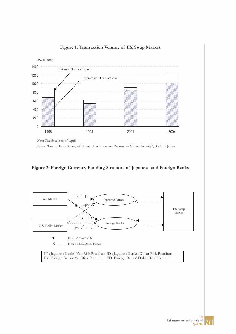
271ECB
Risk measurement and systemic riskApril 2007
Figure 1: Transaction Volume of FX Swap Market
Customer Transactions
Inter-dealer Transactions
US$ billions
Note: The data is as of April.Source: “Central Bank Survey of Foreign Exchange and Derivatives Market Activity”, Bank of Japan
Figure 2: Foreign Currency Funding Structure of Japanese and Foreign Banks
(iv) +FD*i
(iii) +JD*i
(ii) +FYi
(i) +JYiYen Market
U.S. Dollar Market
FX Swap Market
Japanese Banks
Flow of Yen Funds
Flow of U.S. Dollar Funds
Foreign Banks
JY : Japanese Banks’ Yen Risk Premium JD : Japanese Banks’ Dollar Risk PremiumFY: Foreign Banks’ Yen Risk Premium FD: Foreign Banks’ Dollar Risk Premium

272ECBRisk measurement and systemic riskApril 2007
Figure 3: Risk Premiums
(i) Risk Premiums for Japanese Banks
(ii) Risk Premiums for Foreign Banks
(iii) Difference in Risk Premiums between Dollar and Yen Markets
JY : Japanese Banks’ Yen Risk Premium JD : Japanese Banks’ Dollar Risk PremiumFY: Foreign Banks’ Yen Risk Premium FD: Foreign Banks’ Dollar Risk Premium

273ECB
Risk measurement and systemic riskApril 2007
Figure 4: Estimation Results of Factor Analysis (ii)
(i) Factor Loadings
(ii) Time-Series Movement of Each Factor
JD JY FY FD
0.0
0.4
0.8
Factor1
FD FY JY JD
-0.4
0.2
0.6
Factor2
FY JD FD JY
-0.10
0.05
Factor3
Factor 1 (Global Factor)
-2
0
2
4
6
Aug
-92
Aug
-93
Aug
-94
Aug
-95
Aug
-96
Aug
-97
Aug
-98
Aug
-99
Aug
-00
Aug
-01
Aug
-02
Aug
-03
Aug
-04
Factor 3 (Credit Factor)
-6
-4
-2
0
2
4
6
Aug
-92
Aug
-93
Aug
-94
Aug
-95
Aug
-96
Aug
-97
Aug
-98
Aug
-99
Aug
-00
Aug
-01
Aug
-02
Aug
-03
Aug
-04
Factor 2 (Curreny Factor)
-6-4-20246
Aug
-92
Aug
-93
Aug
-94
Aug
-95
Aug
-96
Aug
-97
Aug
-98
Aug
-99
Aug
-00
Aug
-01
Aug
-02
Aug
-03
Aug
-04

274ECBRisk measurement and systemic riskApril 2007
Figure 5: Shadow and Fundamental Prices of Credit Risk
(i) Japanese Banks (JBs)
0.0
0.2
0.4
0.6
0.8A
ug-9
2
Aug
-93
Aug
-94
Aug
-95
Aug
-96
Aug
-97
Aug
-98
Aug
-99
Aug
-00
Aug
-01
Aug
-02
Aug
-03
Aug
-04
0
3
6
9
12
15
JYPRICE (left scale)
JDPRICE (left scale)
Shadow Price of Credit Risk for JBs (right scale)
(ii) Foreign Banks (FBs)
0.0
0.1
0.2
0.3
0.4
0.5
0.6
Aug
-92
Aug
-93
Aug
-94
Aug
-95
Aug
-96
Aug
-97
Aug
-98
Aug
-99
Aug
-00
Aug
-01
Aug
-02
Aug
-03
Aug
-04
29
30
31
32
33
FYPRICE (left scale)
FDPRICE (left scale)
Shadow Price of Credit Risk for FBs (right scale)
JYPRICE : Fundamental Price of Credit Risk for Japanese Banks in the Yen MarketJDPRICE : Fundamental Price of Credit Risk for Japanese Banks in the Dollar MarketFYPRICE : Fundamental Price of Credit Risk for Foreign Banks in the Yen MarketFDPRICE : Fundamental Price of Credit Risk for Foreign Banks in the Dollar Market

275ECB
Risk measurement and systemic riskApril 2007
Figure 6: Generalized Impulse Response Functions (i)
-.005
.000
.005
.010
.015
.020
.025
.030
25 50 75 100 125 150 175 200 225 250
JYJD
FYFD
Response of JY to Generalized OneS.D. Innovations
.00
.01
.02
.03
.04
.05
.06
25 50 75 100 125 150 175 200 225 250
JYJD
FYFD
Response of JD to Generalized OneS.D. Innovations
-.005
.000
.005
.010
.015
.020
.025
.030
25 50 75 100 125 150 175 200 225 250
JYJD
FYFD
Response of FY to Generalized OneS.D. Innovations
-.01
.00
.01
.02
.03
.04
.05
.06
25 50 75 100 125 150 175 200 225 250
JYJD
FYFD
Response of FD to Generalized OneS.D. Innovations
JY : Japanese Banks’ Yen Risk Premium JD : Japanese Banks’ Dollar Risk PremiumFY: Foreign Banks’ Yen Risk Premium FD: Foreign Banks’ Dollar Risk Premium
Note: Impulse response functions are based on the estimation results of the VAR model reported in Table 4(i).

276ECBRisk measurement and systemic riskApril 2007
Figure 7 : Conditional Correlations by M-GARCH Model (i)
JY vs. FY
-1.0
-0.5
0.0
0.5
1.0
Aug
-92
Aug
-93
Aug
-94
Aug
-95
Aug
-96
Aug
-97
Aug
-98
Aug
-99
Aug
-00
Aug
-01
Aug
-02
Aug
-03
Aug
-04
JY vs. JD
-1.0
-0.5
0.0
0.5
1.0
Aug
-92
Aug
-93
Aug
-94
Aug
-95
Aug
-96
Aug
-97
Aug
-98
Aug
-99
Aug
-00
Aug
-01
Aug
-02
Aug
-03
Aug
-04
JD vs. FY
-1.0
-0.5
0.0
0.5
1.0
Aug
-92
Aug
-93
Aug
-94
Aug
-95
Aug
-96
Aug
-97
Aug
-98
Aug
-99
Aug
-00
Aug
-01
Aug
-02
Aug
-03
Aug
-04
JY vs. FD
-1.0
-0.5
0
0.5
0
ug-9
2
ug-9
3
ug-9
4
ug-9
5
ug-9
6
ug-9
7
ug-9
8
ug-9
9
ug-0
0
ug-0
1
ug-0
2
ug-0
3
ug-0
4
1.
0.
A A A A A A A A A A A A A
JD vs. FD
-1.0
-0.5
0.0
0.5
1.0
Aug
-92
Aug
-93
Aug
-94
Aug
-95
Aug
-96
Aug
-97
Aug
-98
Aug
-99
Aug
-00
Aug
-01
Aug
-02
Aug
-03
Aug
-04
FY vs. FD
-1.0
-0.5
0.0
0.5
1.0
Aug
-92
Aug
-93
Aug
-94
Aug
-95
Aug
-96
Aug
-97
Aug
-98
Aug
-99
Aug
-00
Aug
-01
Aug
-02
Aug
-03
Aug
-04
JY : Japanese Banks’ Yen Risk Premium JD : Japanese Banks’ Dollar Risk PremiumFY: Foreign Banks’ Yen Risk Premium FD: Foreign Banks’ Dollar Risk Premium

277ECB
Risk measurement and systemic riskApril 2007
Figure 8: Stability Test of Cointegrating Relationships
(i) Trace Statistic
0
1
2
3
4
5
6
7
8
Aug
-94
Feb-
95
Aug
-95
Feb-
96
Aug
-96
Feb-
97
Aug
-97
Feb-
98
Aug
-98
Feb-
99
Aug
-99
Feb-
00
Aug
-00
Feb-
01
Aug
-01
Feb-
02
Aug
-02
H0: r 0H0: r 1H0: r 2
(ii) Maxmum Eigenvalue Statistic
0
1
2
3
4
5
6
7
8
9
10
Aug
-94
Feb-
95
Aug
-95
Feb-
96
Aug
-96
Feb-
97
Aug
-97
Feb-
98
Aug
-98
Feb-
99
Aug
-99
Feb-
00
Aug
-00
Feb-
01
Aug
-01
Feb-
02
Aug
-02
H0: r 0
H0: r 1
H0: r 2
Notes: 1. r denotes the number of cointegrating ranks.2. Test statistics are divided by the critical values that correspond to the 5% significance level. Thus,
statistics above 1 means that null hypotheses H0 can be rejected at the 5% significance level.3. Time scale corresponds to the mid-period of the rolling window (1,000 observations).

278ECBRisk measurement and systemic riskApril 2007
Figure 9: Generalized Impulse Response Functions (ii)
-.004
-.002
.000
.002
.004
.006
.008
25 50 75 100 125 150 175 200 225 250
JYPRICEJDPRICE
FYPRICEFDPRICE
Response of JYPRICE to Generalized OneS.D. Innovations
-.008
-.004
.000
.004
.008
.012
.016
25 50 75 100 125 150 175 200 225 250
JYPRICEJDPRICE
FYPRICEFDPRICE
Response of JDPRICE to Generalized OneS.D. Innovations
-.002
-.001
.000
.001
.002
.003
.004
.005
25 50 75 100 125 150 175 200 225 250
JYPRICEJDPRICE
FYPRICEFDPRICE
Response of FYPRICE to Generalized OneS.D. Innovations
-.004
-.002
.000
.002
.004
.006
.008
.010
.012
25 50 75 100 125 150 175 200 225 250
JYPRICEJDPRICE
FYPRICEFDPRICE
Response of FDPRICE to Generalized OneS.D. Innovations
JYPRICE : Fundamental Price of Credit Risk for Japanese Banks in the Yen MarketJDPRICE : Fundamental Price of Credit Risk for Japanese Banks in the Dollar MarketFYPRICE : Fundamental Price of Credit Risk for Foreign Banks in the Yen MarketFDPRICE : Fundamental Price of Credit Risk for Foreign Banks in the Dollar Market
Note: Impulse response functions are based on the estimation results of the error correction model reported in Table 9(i).

279ECB
Risk measurement and systemic riskApril 2007
Figure 10 : Conditional Correlations by M-GARCH Model (ii)
JYPRICE vs. FYPRICEJYPRICE vs. JDPRICE
0.95
0.96
0.97
0.98
0.99
1.00
g-92
g-93
g-94
g-95
g-96
g-97
g-98
g-99
g-00
g-01
g-02
g-03
g-04
Au
Au
Au
Au
Au
Au
Au
Au
Au
Au
Au
Au
Au
-1.0
.5
0
1.0
ug-9
2
ug-9
3
ug-9
4
ug-9
5
ug-9
6
ug-9
7
ug-9
8
ug-9
9
ug-0
0
ug-0
1
ug- 0
2
ug-0
3
ug-0
4
0.5
0.
-0
A A A A A A A A A A A A A
JYPRICE vs. FDPRICE
.0
.5
0.0
0.5
0
Aug
-92
Aug
-93
Aug
-94
Aug
-95
Aug
-96
Aug
-97
Aug
-98
Aug
-99
Aug
-00
Aug
-01
Aug
-02
Aug
-03
Aug
-04
JDPRICE vs. FYPRICE
-1.0
-0.5
0.0
0.5
0
Aug
-92
Aug
-93
Aug
-94
Aug
-95
Aug
-96
Aug
-97
Aug
-98
Aug
-99
Aug
-00
Aug
-01
Aug
-02
Aug
-03
Aug
-04
1.1.
-0
-1
JDPRICE vs. FDPRICE
-1.0
-0.5
0.0
0.5
1.0
Aug
-92
Aug
-93
Aug
-94
Aug
-95
Aug
-96
Aug
-97
Aug
-98
Aug
-99
Aug
-00
Aug
-01
Aug
-02
Aug
-03
Aug
-04
FYPRICE vs. FDPRICE
-1.0
-0.5
0.0
0.5
1.0
Aug
-92
Aug
-93
Aug
-94
Aug
-95
Aug
-96
Aug
-97
Aug
-98
Aug
-99
Aug
-00
Aug
-01
Aug
-02
Aug
-03
Aug
-04
JYPRICE : Fundamental Price of Credit Risk for Japanese Banks in the Yen MarketJDPRICE : Fundamental Price of Credit Risk for Japanese Banks in the Dollar MarketFYPRICE : Fundamental Price of Credit Risk for Foreign Banks in the Yen MarketFDPRICE : Fundamental Price of Credit Risk for Foreign Banks in the Dollar Market

280ECBRisk measurement and systemic riskApril 2007
Abstract
This paper considers a simple model of credit risk and derives the limit distribution of losses
under di erent assumptions regarding the structure of systematic and idiosyncratic risks and
the nature of rm heterogeneity. It documents a rich and complex interaction between the un-
derlying model parameters and the resulting loss distributions. The theoretical results indicate
that neglecting heterogeneity in rm returns and/or default thresholds leads to underestimation
of expected losses (EL), and its e ect on portfolio risk is ambiguous. But once EL is controlled
for, neglecting parameter heterogeneity leads to overestimation of risk. These results are veri-
ed empirically where it is shown that heterogeneity in the default threshold or unconditional
probability of default, measured for instance by a credit rating, is of rst order importance in
a ecting the shape of the loss distribution: including ratings heterogeneity alone results in a
more than one-quarter drop in loss volatility and a more than one-half drop in 99.9% VaR, the
level to which the risk weights of the New Basel Accord are calibrated.
JEL Classi cations: C33, G13, G21.
Key Words: Risk management, correlated defaults, factor models, portfolio choice.
FIRM HETEROGENEITY AND CREDIT RISK DIVERSIFICATION*
SAMUEL G . HANSON†
M. HASHEM PESARAN#
TIL SCHUERMANN‡
March 2006
* We would like to thank Richard Cantor, Paul Embrechts, Rafael Repullo, Joshua Rosenberg, Jose Scheinkman,Zhenyu Wang, and especially David Lando, as well as participants at the 13th Annual Conference on Pacific BasinFinance, Economics, and Accounting at Rutgers University, June 2005, the BIS-ECB 4th Joint Central Bank ResearchConference in Frankurt, November 2005, the NBER conference on Risks of Financial Institutions, Cambridge, MA,November 2005, and seminar participants at the Newton Institute, University of Cambridge, UMass Amherst andthe Federal Reserve Bank of New York for helpful comments and suggestions. We are also grateful to Yue Chen andChris Metli for research assistance.† PhD Program in Business Economics, Harvard University, Dept. of Economics and Harvard Business School.Harvard University, [email protected]†# University of Cambridge and USC, [email protected]‡ Corresponding author. Any views expressed represent those of the authors only and not necessarily those of theFederal Reserve Bank of New York or the Federal Reserve System.Federal Reserve Bank of New York and Wharton Financial Institutions Center, [email protected]

281ECB
Risk measurement and systemic riskApril 2007
Abstract
We present new evidence on disaggregated profit and loss and VaR forecasts obtained from a large international commercial bank. Our dataset includes daily P/L generated by four separate business lines within the bank. All four business lines are involved in securities trading and each is observed daily for a period of at least two years. We also collected the corresponding daily, 1-day ahead VaR forecasts for each business line. Given this rich dataset, we provide an integrated, unifying framework for assessing the accuracy of VaR forecasts. Our approach includes many existing backtesting techniques as special cases. In addition, we describe some new tests which are suggested by our framework. A thorough Monte Carlo comparison of the various methods is conducted to provide guidance as to which of these many tests have the best finite-sample size and power properties.
# Christoffersen acknowledges financial support from FQRSC, IFM2, and SSRHC and Pelletier acknowledges financial support from the North Carolina State University Edwin Gill Research Grant. Address correspondence to: Jeremy Berkowitz, Bauer College of Business, 334 Melcher Hall, University of Houston, Houston, Texas, 77204. 1 University of Houston 2 McGill University 3 North Carolina State University
EVALUATING VALUE-AT-RISK MODELS WITH DESK-LEVEL DATA#
JEREMY BERKOWITZ1
PETER CHRISTOFFERSEN2
DENIS PELLETIER3

282ECBRisk measurement and systemic riskApril 2007
SESSION 6
STRESS TESTING
AND FINANCIAL STABILITY POLICY

283ECB
Risk measurement and systemic riskApril 2007
MATHIAS DREHMANN†
BANK OF ENGLAND
ANDREW J. PATTON‡
LONDON SCHOOL OF ECONOMICSAND BANK OF ENGLAND
STEFFEN SORENSEN§
BANK OF ENGLAND
NON-LINEARITIES AND STRESS TESTING

284ECBRisk measurement and systemic riskApril 2007

285ECB
Risk measurement and systemic riskApril 2007

286ECBRisk measurement and systemic riskApril 2007

287ECB
Risk measurement and systemic riskApril 2007
288ECBRisk measurement and systemic riskApril 2007

289ECB
Risk measurement and systemic riskApril 2007
290ECBRisk measurement and systemic riskApril 2007
291ECB
Risk measurement and systemic riskApril 2007
292ECBRisk measurement and systemic riskApril 2007

293ECB
Risk measurement and systemic riskApril 2007

294ECBRisk measurement and systemic riskApril 2007

295ECB
Risk measurement and systemic riskApril 2007

296ECBRisk measurement and systemic riskApril 2007

297ECB
Risk measurement and systemic riskApril 2007
-4 -3 -2 -1 0 1 2 3 4-4
-3
-2
-1
0
1
2
3
4Conditional mean of Y[t] given Y[t-1]
Y[t-1]
TrueLinear approximationQuadratic approximationN(0,1) density

298ECBRisk measurement and systemic riskApril 2007
0 10 20 30 40 50 60 70 80 90 100-2.5
-2
-1.5
-1
-0.5
0
0.5
1
1.5
2
time
Y[t
]
Simulated sample path for Y
1995 2000 2005
4
5
6
7 Interest Rate
1995 2000 2005
0.0
2.5
5.0
7.5 Inflation
1995 2000 2005
2
3
4
5
6GDP growth
1995 2000 2005
1.0
1.5
2.0
2.5Corporate liquidation rate

299ECB
Risk measurement and systemic riskApril 2007
2 4 6 8
-0.1
0
0.1
response of..gdp..to..gdp..shock
2 4 6 8
-0.1
0
0.1
response of..gdp..to..inflation..shock
2 4 6 8
0
0.05
0.1
horizon
response of..gdp..to..int rate..shock
2 4 6 8
-0.2
-0.1
0
0.1
response of..inflation..to..gdp..shock
2 4 6 8
-0.2
0
0.2
response of..inflation..to..inflation..shock
2 4 6 8
-0.1
-0.05
0
0.05
response of..inflation..to..int rate..shock
2 4 6 8
0
0.1
0.2
horizon
response of..int rate..to..gdp..shock
2 4 6 8
0
0.05
0.1
horizon
response of..int rate..to..inflation..shock
2 4 6 80
0.05
0.1
horizon
response of..int rate..to..int rate..shock
2 4 6 8-0.2
-0.1
0
0.1
response of..gdp..to..gdp..shock
2 4 6 8
-0.1
0
0.1
response of..gdp..to..inflation..shock
2 4 6 8-0.1
-0.05
0
0.05
horizon
response of..gdp..to..int rate..shock
2 4 6 8
-0.1
0
0.1
0.2
0.3
response of..inflation..to..gdp..shock
2 4 6 8
-0.2
0
0.2
response of..inflation..to..inflation..shock
2 4 6 8
-0.1
0
0.1
response of..inflation..to..int rate..shock
2 4 6 8
-0.15
-0.1
-0.05
0
0.05
horizon
response of..int rate..to..gdp..shock
2 4 6 8
-0.1
-0.05
0
horizon
response of..int rate..to..inflation..shock
2 4 6 8-0.15
-0.1
-0.05
0
horizon
response of..int rate..to..int rate..shock

300ECBRisk measurement and systemic riskApril 2007
2 4 6 8-1
0
1
response of..gdp..to..gdp..shock
2 4 6 8-0.4-0.2
00.20.40.6
response of..gdp..to..inflation..shock
2 4 6 8-0.2
0
0.2
0.4
horizon
response of..gdp..to..int rate..shock
2 4 6 8
-1
0
1
response of..inflation..to..gdp..shock
2 4 6 8
-0.5
0
0.5
response of..inflation..to..inflation..shock
2 4 6 8
-0.4
-0.2
0
0.2
response of..inflation..to..int rate..shock
2 4 6 8
-0.2
0
0.2
0.4
0.6
horizon
response of..int rate..to..gdp..shock
2 4 6 8
0
0.2
0.4
0.6
horizon
response of..int rate..to..inflation..shock
2 4 6 8
0
0.1
0.2
0.3
horizon
response of..int rate..to..int rate..shock
2 4 6 8
-2
-1
0
1
response of..gdp..to..gdp..shock
2 4 6 8-0.6
-0.4
-0.2
0
0.2
0.4
response of..gdp..to..inflation..shock
2 4 6 8
-0.2
0
0.2
horizon
response of..gdp..to..int rate..shock
2 4 6 8
-4
-2
0
2
4
response of..inflation..to..gdp..shock
2 4 6 8-1
0
1
response of..inflation..to..inflation..shock
2 4 6 8
-0.4
-0.2
0
0.2
response of..inflation..to..int rate..shock
2 4 6 8-0.5
0
0.5
1
horizon
response of..int rate..to..gdp..shock
2 4 6 8
-0.4
-0.2
0
0.2
horizon
response of..int rate..to..inflation..shock
2 4 6 8-0.4
-0.2
0
horizon
response of..int rate..to..int rate..shock

301ECB
Risk measurement and systemic riskApril 2007
2 4 6 80.7
0.8
0.9
1
1.1
1.2
1.3
1.4
gdp
linear
2 4 6 80.7
0.8
0.9
1
1.1
1.2
1.3
1.4
gdp
cubic
2 4 6 80.7
0.8
0.9
1
1.1
1.2
1.3
1.4
infla
tion
2 4 6 80.7
0.8
0.9
1
1.1
1.2
1.3
1.4
infla
tion
2 4 6 80.7
0.8
0.9
1
1.1
1.2
1.3
1.4
int r
ate
horizon2 4 6 8
0.7
0.8
0.9
1
1.1
1.2
1.3
1.4
int r
ate
horizon

302ECBRisk measurement and systemic riskApril 2007
2 4 6 80.40.60.8
11.21.41.61.8
22.2
gdp
linear
2 4 6 80.40.60.8
11.21.41.61.8
22.2
gdp
cubic
2 4 6 8
0.6
0.8
1
1.2
1.4
1.6
1.8
2
infla
tion
2 4 6 8
0.6
0.8
1
1.2
1.4
1.6
1.8
2
infla
tion
2 4 6 80.8
1
1.2
1.4
1.6
int r
ate
horizon2 4 6 8
0.8
1
1.2
1.4
1.6
int r
ate
horizon

303ECB
Risk measurement and systemic riskApril 2007
2 4 6 80.7
0.8
0.9
1
1.1
1.2
1.3
1.4
gdp
linear
2 4 6 80.7
0.8
0.9
1
1.1
1.2
1.3
1.4
gdp
cubic
2 4 6 80.7
0.8
0.9
1
1.1
1.2
1.3
1.4
infla
tion
2 4 6 80.7
0.8
0.9
1
1.1
1.2
1.3
1.4in
flatio
n
2 4 6 80.7
0.8
0.9
1
1.1
1.2
1.3
1.4
int
rate
horizon2 4 6 8
0.7
0.8
0.9
1
1.1
1.2
1.3
1.4
int
rate
horizon

304ECBRisk measurement and systemic riskApril 2007
2 4 6 80
1
2
3
4
5
6
7
gdp
linear
2 4 6 80
1
2
3
4
5
6
7
gdp
cubic
2 4 6 80.5
0.75
1
1.25
1.5
1.75
2
infla
tion
2 4 6 80.5
0.75
1
1.25
1.5
1.75
2
infla
tion
2 4 6 80.4
0.5
0.6
0.7
0.8
0.9
1
1.1
1.2
int r
ate
horizon2 4 6 8
0.4
0.5
0.6
0.7
0.8
0.9
1
1.1
1.2
int r
ate
horizon
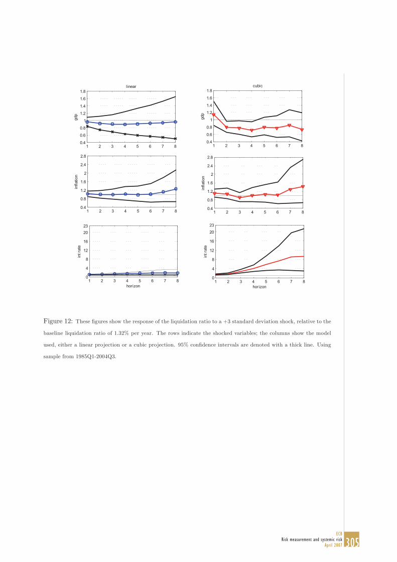
305ECB
Risk measurement and systemic riskApril 2007
1 2 3 4 5 6 7 80.4
0.6
0.8
1
1.2
1.4
1.6
1.8
gdp
linear
1 2 3 4 5 6 7 80.4
0.8
1.2
1.6
2
2.4
2.8
infla
tion
1 2 3 4 5 6 7 80
4
8
12
16
20
23
horizon
int r
ate
1 2 3 4 5 6 7 80.4
0.6
0.8
1
1.2
1.4
1.6
1.8
gdp
cubic
1 2 3 4 5 6 7 80.4
0.8
1.2
1.6
2
2.4
2.8
infla
tion
1 2 3 4 5 6 7 80
4
8
12
16
20
23
int r
ate
horizon

306ECBRisk measurement and systemic riskApril 2007
2 4 6 80 . 4
0 . 7
1
1 . 3
1 . 6
1 . 8 5gd
p
l i n e a r
2 4 6 8
1
2
3
4
5
infla
tion
2 4 6 80
0 . 4
0 . 8
1 . 2
1 . 5
h o r i z o n
int
rate
2 4 6 80 . 4
0 . 7
1
1 . 3
1 . 6
1 . 8 5
gdp
c u b i c
2 4 6 8
1
2
3
4
5
infla
tion
2 4 6 80
0 . 4
0 . 8
1 . 2
1 . 5
int
rate
h o r i z o n
307ECB
Risk measurement and systemic riskApril 2007

308ECBRisk measurement and systemic riskApril 2007

309ECB
Risk measurement and systemic riskApril 2007
Abstract
In this paper we empirically study interactions between real activity and the financial stance. Usingaggregate data we examine a number of candidate measures of the financial stance of the economy. Wefind strong evidence for substantial spillover effects on aggregate activity from our preferred measure.Given this result, we use a large micro-data set for corporate firms to develop a macro–micro-modelof the interaction between the financial and real economy. This approach implies that the impulseresponses of a given aggregate shock will depend on the portfolio structure of firms at any given pointin time.© 2005 Elsevier B.V. All rights reserved.
JEL classification: C41; G21; G33; G38
Keywords: Default-risk models; Business cycles; Financial stability; Price stability; Financial and real economyinteraction
� We have benefitted from comments by participants at the “Regulation and Financial Stability Conference” atthe Federal Reserve Bank of Atlanta (23–24 September 2004), especially our discussant Charles Evans. Moreover,we have benefitted from presentations at the BIS 2003 autumn economist meeting on “The interaction between thefinancial and real side of the economy”, University of Verona and the Bank of England workshop on macro-stresstesting. Special thanks to Rikard Nilsson for superb research assistance. The views expressed in this paper aresolely the responsibility of the authors and should not be interpreted as reflecting the views of the Executive Boardof Sveriges Riksbank.
∗ Corresponding author.E-mail address: [email protected] (T. Jacobson).
EXPLORING INTERACTIONS BETWEEN REAL ACTIVITY AND THE FINANCIAL STANCE
TOR JACOBSON*, JESPER LINDÉ, KASPER ROSZBACH

310ECBRisk measurement and systemic riskApril 2007
1. Introduction
In this paper we empirically study the interactions between Swedish firms’ balance sheetsand the evolution of the Swedish economy. Most economists would consider it triviallytrue that macroeconomic conditions influence the state of the firms’ balance sheets: goodtimes result in prosperous firms with strong balance sheets, likewise a slowdown in theeconomy will be reflected by weak balance sheets. In that same view, the evolution of themacroeconomy will ultimately be determined by its firms’ relative successes. Nevertheless,quantifying such relationships has turned out to be non-trivial. Most research has focusedon either identifying the impact of macroeconomic conditions on firms’ balance sheets,or the consequences of firms’ balance sheets (generally through a bank channel) on themacroeconomy. The purpose of this paper is to explore the interaction and feedback betweenfirms’ balance sheets and the macroeconomy. It turns out that by using aggregate credit risk,approximated by firms’ bankruptcy frequency over time, we find a useful link between themicro- and the macro-perspective.
Among policymakers, there appears to exist a broad consensus that market imperfectionsand instability in the financial sector can have significant and long-lasting effects on thereal economy, cf. Lowe (2001). For academics, however, the role of the financial sector andcredit in the macroeconomy has been a source of frequent debate, with some economists,see e.g. Poole (1993) arguing that credit only plays a role of its own in periods of financialcrises. Others, see e.g. Bernanke (1993) and Calomiris and Glenn Hubbard (1989), hold thatcredit markets generally and continuously affect the macroeconomy through the so-calledcredit channel.
Bernanke and Gertler (1995) describe the credit channel as “set of factors that amplifyand propagate conventional interest rate effects” of monetary policy through endogenouschanges in the external finance premium. Adherents of this “credit view” have identi-fied two main linkages between central banks’ actions and credit markets: a (borrowers’)balance-sheet channel and a bank lending channel.1 The first link stresses the importance ofborrowers’ balance sheets and income statements, acknowledging that changes in monetarypolicy will have an impact on variables such as borrowers’ net worth, cash flow and liquidassets. A second transmission mechanism focuses on the potential effect of monetary policyon the supply of loans by financial institutions. A common premise is, however, that fric-tions interfere with the smooth functioning of financial markets, creating a wedge betweenthe cost of externally raised funds and the opportunity cost of internal funds.
A large number of studies has explained and tested the mechanisms by which shocks tothe financial sector are propagated into the real sector of the economy and found evidencein support of the existence of a balance-sheet channel. As far as the bank lending channelis concerned, the evidence in favor and against is still very much under debate. One of thestudies that revived the debate on the balance-sheet channel is Bernanke (1983). In his studyof non-monetary effects of the financial crisis during the Great Depression, he contendsthat the financial crisis of the 1930s “affected the macroeconomy by reducing the quality ofcertain financial services, primarily credit intermediation”, which in its turn disrupted the
1 The balance sheet channel has sometimes also been called the broad credit channel. See for example Repulloand Suarez (2000).
311ECB
Risk measurement and systemic riskApril 2007
normal flow of bank credit. He also brings forward evidence of how the increase in defaultsand bankruptcies and the progressive erosion of borrowers’ collateral relative to their debtburdens during this period increased the cost of credit intermediation. Banks reacted to thesechanges by stopping to make loans to lower-quality investors, to which they had lent before.2
The events in the financial sector ultimately affected the bearing of the macroeconomybecause the resulting higher effective cost of credit reduced businesses demand for current-period goods and services. An analysis of the determinants of output by Bernanke shows thattwo proxies for the financial crisis—changes in the deposits of failing banks and changesin the liabilities of failing businesses have substantial additional explanatory power for thegrowth rate of industrial production. In related work Coe (2002) use a Markov switchingmodel to estimate conditional probabilities of a financial crisis occurring. He finds thatthese estimated probabilities have additional explanatory power in an model of real output,evidence that supports Bernanke’s findings. Bernanke and Gertler (1989) develop a smallmodel in which they use the inverse relationship between borrower net worth and theagency costs of investment to explain why changes in the condition of borrowers’ balancesheets can be a source of business cycle fluctuations—without any financial crisis precedingthe shocks.3 In a companion paper, Bernanke and Gertler (1990) also argue that financialfactors can have quantitatively significant real effects by demonstrating how changes in thecreditworthiness of borrowers affect investment spending, expected returns and the overalleconomy.
More recently research efforts have attempted to meet the criticism that earlier studiesof the credit channel failed to isolate supply shocks from demand shocks and persuasivelyestablish the existence of real effects. To avoid identification issues, this later work has testedthe cross-section implications of the credit view. For example, Gertler and Gilchrist (1993,1994) find that larger firms have better access to credit and typically respond to unexpectedadverse conditions by increasing short-term borrowing, while smaller firms instead respondby squeezing inventories and cutting production. Bernanke et al. (1996) obtain similarfindings when they split up firms according to their degree of bank dependency ratherthan based on size. Samolyk (1994) examines the relationship between banking conditionsand economic performance at the US states level and finds that local bank balance-sheetconditions help to predict the performance of regional economies in a way that is consistentwith the existence of credit market imperfections. Ludvigson (1998) uses automobile creditdata from bank and non-bank sources and finds evidence for the presence of a bank lendingchannel. Peek and Rosengren (2000) study the effects of the Japanese banking crisis onconstruction activity in the US. Their work makes clear that the retrenchment of Japaneselending had a substantial impact on US. real estate activity, indicating that at least someborrowers were not able to obtain alternative financing and that credit markets thus weresuffering from imperfections. Repullo and Suarez (2000) develop a theoretical model thatcan compare the macro-implications of both the balance-sheet channel and the bank lendingchannel and conclude that the presence of a balance-sheet channel is most likely.
2 An important indicator of this phenomenon is the bond spread between Baa corporate bonds and Treasurybonds, that increased from 2.5% in 1929–1930 to nearly 8% in mid-1932. See Bernanke (1983) p. 266.
3 Bernanke and Gertler (1990) define financial instability (“fragility”) as a situation in which potential borrowershave low wealth relative to the sizes of their projects.
312ECBRisk measurement and systemic riskApril 2007
This paper is closely related to the above work as we study the interaction between realactivity and firms’ balance sheets. Unlike earlier studies, however, that primarily seek toidentify a one-way linkage between the macroeconomy and financial markets, we combinea microeconometric model of firms’ financial default behavior and a macroeconometricmodel to study how macro-aggregates and the aggregate effects of changes in individualfirms’ balance sheets and income statements interact with each other. Our focus is less on theexistence of a “credit channel” but rather on the interaction between the economy’s financialstance at the firm level and the economy’s aggregate behavior. Although our link betweenmicro-conditions and the macro-model is not derived from micro-foundations, we believethat this eclectic approach offers a number of advantages. For one thing, we will be able toinvestigate if macroeconomic policy will affect businesses equally, both cross-sectionallyand through time. We will also be able to look into the relative importance of firm-specificand aggregate disturbances.4
We model the macroeconomy by a set of macroeconomic variables, including the aggre-gate bankruptcy frequency, in a quarterly vector autoregressive model. Furthermore, theimpact of firms’ balance-sheet variables on bankruptcy risk is modeled in a dynamic paneldata model, where we also condition on macroeconomic variables. To this end we have col-lected an extensive data set containing balance-sheet information on the entire populationof Swedish incorporated firms (some quarter of a million firms) for 40 consecutive quarters,1990Q1 – 1999Q2 (in total, close to 8 million firm-observations). This sample period coversthe “banking crisis” period in Sweden (1991–1993) and also a benign period characterizedby high growth in the late 1990s.
The empirical model is a system made up of three blocks. The first one is a vectorautoregressive (VAR) model for the macroeconomic variables we consider. Based on workby Linde (2002), we choose to include the following endogenous variables in the VAR;output, inflation, the nominal interest rate (the REPO rate), and the real exchange rate.Since Sweden is a small open economy it is necessary to condition on a set of foreignvariables that enters the model exogenously. As another exogenous variable in the VAR weinclude our preferred measure of the financial stance, the aggregated default frequency ofincorporated firms, a variable that is highly positively correlated with the banking sectorcredit losses during the 1990s. An important first step in the analysis is to use a multivariateGranger-causality test, or block-exogeneity test, in order to examine what extent variousfinancial indicator variables are helpful predictors of the macroeconomy. This exercise isundertaken for a larger set of financial variables, and we find that the aggregate defaultfrequency is the most important one.
In the second block we have a logit model for the default risk at the firm level wherethe macroeconomic variables as well as various balance-sheet variables enter as regressors.The logit model will carefully follow the methods that have been applied in earlier studieson company default, such as Altman and Saunders (1997), Shumway (2001) and Carling etal. (2004). Let Di,t denote default status of firm i in period t. By computing
(∑i Di,t
)/Nt ,
where Nt is the number of firms each time period, we retrieve a time-series of the aggregate
4 Although we are aware of the importance of job and business creation, our focus here is on interaction betweenthe macroeconomy and business default (destruction).

313ECB
Risk measurement and systemic riskApril 2007
default frequency that can be inserted into the VAR-model. So, once equipped with a VAR-model and the estimated logit model, we can simulate the effects of various disturbances inthe economy. For instance, we can study the dynamic effects of a shock to monetary policyon inflation and the default frequency in a joint framework.
The third block in the empirical model is an attempt to estimate how the balance-sheetvariables that are included in the logit model depend on the macroeconomic variables.Due to the panel-data nature of our firm-level data set, we estimate a dynamic panel VAR-type model for the balance-sheet variables (that are included in the logit model) letting themacro-variables enter as regressors. We can then study if the macroeconomic variables arequantitatively important for explaining variation in the balance-sheet variables.
Our main findings are as follows. First, we find that the aggregate default frequency isa significantly and quantitatively important link from the financial to the real side of theeconomy, whereas other commonly considered financial indicators appear less so. Second,we find that macroeconomic variables are important for explaining a time-varying defaultfrequency. Firm-specific variables are very useful in ranking the riskness of firms, butmacroeconomic variables are of crucial importance for explaining changes in absolutedefault risk. Third, most of the variation in balance-sheet variables are of idiosyncraticorigin. Fourth, the empirical model implies that the effects of monetary policy on thedefault frequency and the inflation rate are state dependent: monetary policy appears tobe more potent under recessions than during booms. Finally, we find that our empiricalmodel appears to more accurately produce joint forecasts of inflation and the aggregatedefault frequency in comparison to a standard VAR-model where the default frequency isincluded as an endogenous variable.
The remainder of this paper is structured as follows. In the next section, we presentour micro- and macro-data sets. The dependency of the real side of the economy on theset of financial variables we study is examined in Section 3. In Section 4, we test for thedependency of the financial variables for the macro-variables. In Section 5, we summarizethe empirical models that are used to examine the interaction between the real and financialside of the economy. The empirical micro–macro-model is then used in Section 6 to shedlight on some interesting policy issues. In this section, we also compare the properties ofthis model with those of a VAR-model where the aggregate default frequency is includedas an endogenous variable. Finally, Section 7 concludes.
2. Data
2.1. Micro-data
In this subsection, we provide a detailed description of our data set at the firm level.The final data set is a panel consisting of 7,652,609 quarterly observations on incorporated
firms, covering 10 years of quarterly data for all Swedish aktiebolag companies that haveissued a financial statement between 1 January 1990, and 30 June 1999. Aktiebolag areby approximation the Swedish equivalent of US corporations and UK limited businesses.Swedish law requires every aktiebolag to have at least SEK 100,000 (approximately US$10,000) of equity to be eligible for registration at the Swedish Patent and Registration

314ECBRisk measurement and systemic riskApril 2007
Office (PRV). Firms are also required to submit an annual report to PRV. Small firms suchas general partnerships, limited partnerships and sole proprietors will be disregarded, since,as reported by Jacobson and Linde (2000), incorporated firms by far account for the largestfraction of loans and, also, display the most cyclical variation in default risk.
The firm-data come from Upplysningscentralen AB (UC), a major credit bureau in Swe-den, and are from two general sources of information. First, UC has provided us withbalance-sheet and income statement data from the firms’ annual reports submitted to PRV.These annual report data cover the period 1 January 1989–31 December 1999. Second, UChas provided us with historical data on events related to payment remarks and paymentbehavior for the firms and for their principals. The UC-data are available at different fre-quencies, varying from daily for payment remarks to (most often) annually for accountingdata. We will discuss the specifics of the data in greater detail below.
The accounting data contains information on most standard balance-sheet and incomestatement variables. Appendix A5, which is available upon request, contains a complete listof annual report variables. In addition to the annual report data, we have information on thefirms’ track records regarding payment behavior as recorded by remarks for 61 differentcredit and tax related events. The storage and usage of payment remarks are regulated by theCredit Information Act, the Personal Data Act and overseen by the Swedish Data InspectionBoard. Examples of events that are registered are: delays in tax payments, the repossessionof delivered goods, the seizure of property, the resettlement of loans and actual bankruptcy.In practice, with a record of payment remarks individuals will not be granted any new loansand businesses can find it very difficult to open new lines of credit. Appendix B5, which isavailable upon request, contains the complete list of payment remarks.
We define the population of existing firms in quarter t as the firms, which have issueda financial statement covering that quarter and are classified as “active”. For a firm to beclassified as active, we require that is has total sales and total assets over 1000 SEK (roughlyUS$ 100). In addition to these firms, we add the firms which according to the data set onremarks are classified as defaulted firms.6 The adopted definition of default is the one usedby UC.7
In Table 1, we report all descriptive statistics for the employed accounting ratios and othervariables, such as payment remarks and average delayed time to the last issued financialreport for the defaulted and non-defaulted firms. Because of varying availability of data,the statistics in Table 1 were calculated based on different numbers of observations. Forfirms where accounting data are not available, we replace missing values by the panelmean for the defaulted/non-defaulted firms. In part A of Table 1, showing non-truncateddata, there are some accounting data observations that clearly are severe outliers. Theseobservations would seriously distort the estimation results if they were to be included in
5 Available upon request.6 There is a simple reason why we need to add firms that have defaulted to the population of firms defined by the
accounting data. Many firms that default choose not to submit their compulsary annual reports in the year, or evenyears, prior to default. Hence, the only records of their existence that we have come from the remark registers.
7 According to the UC-definition, a firm has default status if any of the following more important events haveoccured: the firm is declared bankrupt in the legal sense, it has suspended payments, it has negotiated a compositionsettlement, it is undergoing a re-construction, or, distraint with no assets. We differ somewhat from the creditbureau’s definition though, in that we use a one quarter horizon, whereas they currently employ a 1-year horizon.

315ECB
Risk measurement and systemic riskApril 2007
Table 1Descriptive statistics for the micro-data
Firm type N µ σ Statistic
min 1% 50% 99% max
Part A: non-truncated dataNon-defaulted 7549041EBITDA/TA 7471212 −0.12 220.40 −256885 −1.03 0.11 0.85 66424TL/TA 7474248 3.56 1351.21 −408 0.03 0.73 2.42 1703742LA/TL 7451325 1.09 109.37 −71203 0 0.13 7.94 54655I/TS 7355762 4.84 6254.23 −26845 0 0.01 2.18 16500000TL/TS 7474248 2.32 120.73 −32.25 0 0.08 17.02 48536IP/(IP + EBITDA) 7457030 −1.7E10 2.8E13 0 −3.59 0.10 3.95 2.2E16Defaulted 103568EBITDA/TA 67093 −6.04 1201.38 −215719 −5.40 0.03 1.23 164895TL/TA 67110 208.17 25784.42 −23304 0.01 0.94 18.97 5407312LA/TL 66729 0.57 24.20 −436 0 0.02 4.87 3258I/TS 63138 27.05 6319 −0.19 0 0.03 5.21 1587085TL/TS 67110 0.80 8.46 −0.08 0 0.12 9.53 787IP/(IP + EBITDA) 66670 0.35 28.53 −1216 −6.09 0.23 6.90 5794
Part B: truncated dataNon-defaulted 7549041EBITDA/TA 7471212 0.11 0.25 −1.05 −1.03 0.11 0.84 0.84TL/TA 7474248 0.71 0.35 0.03 0.03 0.73 2.42 2.46LA/TL 7451325 0.53 1.12 0 0 0.13 7.81 7.81I/TS 7355762 0.12 0.29 0 0 0.01 2.13 2.13TL/TS 7474248 0.58 2.08 0 0 0.08 14.74 18.61IP/(IP + EBITDA) 7457030 0.15 0.76 −3.55 −3.55 0.10 3.91 3.91PAYDIV (%) 7549041 13.15 33.80 0 1REMARK1 (%) 7549041 0.33 5.77 0 1REMARK2 (%) 7549041 3.06 17.21 0 1TTLFS (%) 7549041 1.54 12.30 0 1Defaulted 103568EBITDA/TA 67093 −0.03 0.35 −1.05 −1.05 0.03 0.84 0.84TL/TA 67110 1.00 0.0 0.03 0.03 0.94 2.46 2.46LA/TL 66729 0.21 0.82 0 0 0.02 4.87 7.81I/TS 63138 0.18 0.38 0 0 0.03 2.13 2.13TL/TS 67110 0.57 1.75 0 0 0.12 9.52 18.61IP/(IP + EBITDA) 66670 0.24 0.99 −3.55 −3.55 0.23 3.91 3.91PAYDIV (%) 103568 0.70 8.31 0 1REMARK1 (%) 103568 14.90 35.61 0 1REMARK2 (%) 103568 40.60 49.11 0 1TTLFS (%) 103568 33.42 47.17 0 1
Notes: The definition of variables are: EBITDA = earnings before taxes, interest payments and depreciations;TA = total assets; TL = total liabilities; LA = liquid assets; I = inventories; TS = total sales; IP = sum of net interestpayments on debt and extra-ordinary net income; PAYDIV = a dummy variable equal 1 if the firm has paid outdividends during the accounting period and 0 otherwise; REMARK1 = a dummy variable taking the value of 1 ifthe firm has a payment remark due to one or more of the following events in the preceding four quarters; (i) a“non-performing loan” at a bank, or (ii) a bankruptcy petition, or (iii) issuance of a court order to pay a debt, or(iv) seizure of property; REMARK2 = a dummy variable taking the value of 1 if the firm is in various tax arrears;TTLFS = a dummy variable equal to 1 if the firm has not submitted an annual report in the previous year, and 0otherwise.

316ECBRisk measurement and systemic riskApril 2007
the logit model. Therefore, we have truncated the top and bottom 1% observations for theaccounting variables.8 Given the large number of observations, this approach is more orless equivalent to simply deleting 1% of the observations that have accounting data that falloutside a certain region. Part B of Table 1 shows the descriptive statistics for the truncatedmicro-data set.9
As financial reports issued by firms typically become available with a significant timelag, it cannot in general be assumed that accounting data for year τ are available duringor even at the end of year τ to forecast default risk in year τ + 1. To account for this, wehave lagged all accounting data by four quarters in the estimations. For most firms, whoreport balance-sheet and income data over calendar years, this means that data for year τ isassumed to have been available in the first quarter of year τ + 1.
For a number of firms some transformation had to be applied to the accounting variablesto adjust for reporting periods that did not coincide with the calendar year, to assure thateach variable is measured in identical units for all firms. Some firms, for example, reportaccounting information referring to 3- or 4-month periods for one or several years. In suchcases, annual balance-sheet figures were calculated as weighted averages of the multipleperiod values. In other cases companies did report numbers for a 12-month period, butthe period did not coincide with the calendar year. The 1995 figures, for example, couldrefer to the period 1 April 1995 until 31 March 1996. In these cases, such “deviations” wereaccounted for by adjusting the “four quarter lag” (and thus the date at which the informationis assumed to have been available) correspondingly.
Before we decided to restrict our attention to the set of financial ratios that are shownin Table 1, we studied a number of commonly used accounting ratios that were employedin frequently cited articles studying bankruptcy risk and the balance-sheet channel, but theones reported show the strongest correlation with default risk.10 In our empirical model, weemploy six accounting ratios: earnings before interest, depreciation, taxes and amortizationover total assets (earnings ratio); interest payments over the sum of interest payments andearnings before interest, depreciation, taxes and amortization (interest coverage ratio); totalliabilities over total assets and total liabilities over total sales (debt ratios); cash in relationto total liabilities (cash ratio); and inventories over total sales (turnover ratio).11 These
8 This approach is quite common in the literature, and e.g. Shumway (2001) also truncate 1% of the top andbottom observations. It should be emphazied that the results are not at all sensitive when varying the truncationrate between 0.5 and 2%.
9 From Table 1, comparison of the descriptive statistics for the untruncated data makes it clear that defaulted firmsare unproportionally more affected when truncating all the observations simultaneously. Since the REMARK1,REMARK2, PAYDIV and TTLFS are dummy variables that are unaffected by our truncation procedure, it maylead to underestimation of the importance of the accounting data variables in the default risk model relative tothese dummy variables. To check the robustness of our chosen approach, we used an alternative approach wherewe truncated the healthy and defaulted firms separately. As expected, the estimation results of the default-riskmodel with this alternative truncation suggested a somewhat larger role for the accounting ratios, but the over-allpicture remains the same.10 See Altman (1968, 1971, 1973, 1984), Carling et al. (2004), Frydman et al. (1985), and Shumway (2001).11 It should be noted that the level of debt, in addition to the leverage ratio (TLi,t/TAi,t) for firm i in period t,
appears to contain predictive power for default risk. We therefore decided to include TLi,t as separate variable,but scaled it with average total sales in period t to obtain a stationary accounting ratio. So the debt to sales ratio isactually defined as TLi,t/TSt, where TSt denotes average total sales in period t.

317ECB
Risk measurement and systemic riskApril 2007
Fig. 1. Default rates and the cumulative distribution functions for the accounting data.
six ratios were selected following a two-step procedure. First, the univariate relationshipbetween the ratio and default risk was investigated. By visual inspection, ratios that lackedany correlation with default risk were deleted from the set of candidate explanatory variables.Fig. 1 illustrates this for the six selected ratios by comparing default rates (solid line) andthe cumulative distributions of the variables (dotted line). The default rate for a givenobservation of a ratio is calculated as an average over the interval of ±5000 adjacentobservations in the empirical distribution of the ratio at hand. Given the density of theobservations, there is a positive relationship between default risk and the leverage, interestcoverage and turnover ratios, while the figure suggests a negative relationship for both thedebt and the liquidity ratios. The diagrams in Fig. 1 suggest that the relationship betweendefault-risk and the earnings ratio, total liability over total sales ratio and interest costsover the sum of interest costs and earnings are non-linear. For instance, for the interestcoverage variable, this relationship is perhaps what one would have expected; low (negativeearnings) can turn this ratio highly negative if interest costs are high but earnings areslightly more negative, and this event is naturally associated with an increased defaultrisk.
On the other hand, high interest payments and low earnings will also make this ratiolarge, and is likewise associated with an increased default risk. Similar reasoning can beapplied to the other ratios as well. What is important to note is that this feature for some ofthe financial ratios does not imply that these variables are uninformative for default risk inthe empirical model. The reason for this being that the correlations between these financial
318ECBRisk measurement and systemic riskApril 2007
ratios in the cross section are substantial, which makes each of these variables contributeto predicting default risk in the joint empirical model.12 Taking these insights into account,Fig. 1 confirms the picture emerging from Table 1: there is a clear difference betweenhealthy and defaulted firms for these variables.
For the remark variables, we employ the same approach as in Carling et al. (2004)and use simple dummy variables by setting them to unity if certain remarks existed forthe firm during the year prior to quarter t, and 0 otherwise. An intuitively reasonablestarting point was to find remark events that (i) lead default as much as possible and (ii)are highly correlated with default. As it turned out, many remark variables are eithercontemporaneously correlated with default or lack a significant correlation with defaultbehavior. For our final model, we constructed the REMARK1-variable as a compositedummy of four events: a bankruptcy petition, the issuance of a court order – because ofabsence during the court hearing – to pay a debt, the seizure of property, and “having anon-performing loan”, and the REMARK2-variable reflects if the firm is in various taxarrears. In the accounting data, we also have information whether a firm has paid outdividends or not. We therefore included this information as a dummy variable (PAYDIV)in the model, taking the value of 1 if the firm has paid out dividends and 0 otherwise.
In addition, we have included a dummy variable, denoted TTLFS, which equals unityif a firm has not issued a financial statement one and a half year prior to default, and zerootherwise.13 The reason for including this variable in the default-risk model is the notionthat firms who are about to default are less willing to report information about their financialstatus. By comparing defaulting and healthy firms in Table 1 we see that this mechanism isat work in the panel.
2.2. Macro-data
The macro-data used in this paper is adopted from Linde (2002) and covers the period1986Q3–2002Q4. We restrict the sample to this period because Swedish financial mar-kets were heavily regulated prior to 1986. The domestic variables are yd
t – the output-gap(i.e., deviation of GDP around its trend value), πd
t – the annual inflation rate (measured asthe fourth difference of the GDP-deflator), Rd
t – the REPO nominal interest rate (a short-
12 For instance, taking the square of the interest coverage ratio, which judging by Fig. 1, would seem appropriatein a single variable analysis, reduces the explanatory power of this variable in the multivariate model.13 There are three things worth noting in connection with the definition of TTLFS. First, this information is
assumed to be available with a 6 quarter time lag since financial statements for year τ are typically available inthe third quarter in year τ + 1. By letting this dummy variable equal unity with a 6 quarter time lag we do take thereal-world time delay into account. Second, given the way we define the population of existing firms, firms that arenewly registered and enter into the panel would automatically be assigned TTLFS = 1 in the third quarter of theirexistence since they have not issued any financial statement prior to entering. For these new firms, TTLFS hasbeen set to 0 and the accounting data variables have been taken from their first yearly balance sheet and incomestatements. Third, for defaulting firms that are in the panel but have never reported any accounting data prior todefault, we also set TTLFS equal to 0. This is the case for 38,352 out of 103,568 defaulting firms in the panel. Soalthough TTLFS turns out to be very important in the default-risk model, by construction the importance of thisvariable is down-played rather than exaggerated.

319ECB
Risk measurement and systemic riskApril 2007
Fig. 2. Macro-data used in the estimated VAR-models.
term interest rate, controlled by the Riksbank), and qt – the real exchange rate.14 Becausethere is a strong trend for the real exchange rate during the sample period, this variable isdetrended as well.15 Since Sweden is an open economy, it is important to condition on for-eign variables in the VAR-model. Consequently, we also include yf
t – the foreign output gap(computed by Linde, 2002), πf
t – foreign inflation rate, and Rft – the 3-month nominal inter-
est rate as exogenous variables. To acquire data on the aggregate default frequency, denoteddft for the sample outside the panel period 1990Q1–1999Q2, we linked the panel seriesdepicted in Fig. 2 for 1986Q3–1989Q4 with the aggregate default frequency data for allbusiness firms (made available by Statistics Sweden), and for the period 1999Q3–2002Q4
14 The real exchange rate is measured as the nominal TCW-weighted (TCW = trade competitive weights) exchangerate times the TCW-weighted foreign price level (CPI deflators) divided by the domestic CPI deflator.15 Linde (2002) estimates a VAR with two lags for the period 1986Q3–2002Q4 and generates a trend for the
variables by doing a dynamic simulation of the estimated VAR under the assumption of no shocks hitting theequations. The detrended variables are then computed as actual values minus the trend values. It should be noted,however, that using HP-filtered data for output and the real exchange rate produces very similar results to thosereported.

320ECBRisk measurement and systemic riskApril 2007
with the aggregate default frequency for incorporated firms (again, source StatisticsSweden).
3. The dependency of real variables on financial variables
In this section, we use aggregate data to examine if there is a feedback from the financialside to the real side of the economy. Throughout the analysis, we will work with the VAR-model estimated by Linde (2002) as the tool to study this issue. The VAR(p)-model with plags is specified as
Xt = Cd + δ1D923 + δ2D931013 + τdTt +p∑
i=0
FiZt−i +p∑
i=1
Bd,iXt−i + ud,t , (1)
where D923 is a dummy variable equal to 1 in 1992Q3 and 0 otherwise, D931013 is a dummyvariable equal to 1 in 1993Q1 and thereafter, Tt is a linear time-trend, and Zt is a vectorwith the exogenous variables. The dummy variable for the third quarter in 1992 is includedto capture the exceptionally high interest rate increase (up to 500%) implemented by theRiksbank in order to defend the fixed Swedish exchange rate. Despite the efforts to defendthe Swedish krona, Sweden entered into a floating exchange rate regime in late November1992, and the dummy variable D931013 is included in order to capture possible effects ofthe new exchange rate regime.
The variables in Xt and Zt are
Xt = [yd
t πdt Rd
t qt
]′and Zt = [
yft πf
t Rft
]′. (2)
Linde (2002) shows that two lags is sufficient (i.e., we set p = 2), and that the foreignvariables are block exogenous with respect to the domestic variables, i.e., the variables inZt are not affected by the variables in Xt.
One natural way to test if there is a feedback from the financial sector into the real sideof the economy is to augment the specification in (1) with lags of the financial variable, i.e.,include dft−1 and dft−2 and examine if they contain useful information for predicting theendogenous variables in the model. This has the flavor of a multivariate Granger-causalitytest. Essentially, one simultaneously test if the coefficients for the lags are significantlydifferent from zero or not. By using the block-exogeneity test described in detail by Hamilton(1994), cf. pages 309–312, we find that the p-value for the null of zero coefficients is around0.02, indicating that the macroeconomic variables in Xt are not exogenous with respect tothe aggregate default frequency.
An alternative way to quantify the dependence of the real economy on the defaultfrequency is to include dft, ordered last, in the Xt-vector and estimate a five-variable VAR-model. If the impulse response functions in the estimated VAR-model for a shock to dft,identified via a so-called Cholesky-decomposition, are close to zero, then the quantitativefeedback from the default frequency to the real economy is small. In Fig. 3, we show theimpulse response functions a positive shock to the dft variable. We see that the outcomeof the block-exogeneity test is confirmed, the financial shock has significant effects on thereal economy. Output and inflation falls, while the nominal interest rate increases (although

321ECB
Risk measurement and systemic riskApril 2007
Fig. 3. Impulse response functions to a aggregate default frequency shock in the estimated VAR where defaultfrequency is included in Xt.
not significantly), and the real exchange rate appreciates. According to the VAR, exoge-nous variations in the default rate account for as much as 20% of the variation of the othervariables.
We have also investigated whether the average balance sheets ratios (depicted in Fig. 4)explain the variation in the macrovariables over and above the explanatory power of thedefault rate variable and the other macrovariables included in the VAR. Since we onlyhave data on the balance sheets ratios for the period 1990Q1–1999Q2, we regressed theVAR-residuals for this period on the balance-sheet ratios equation by equation with OLS.A simple F-test revealed that the balance-sheet ratios conveyed no information w.r.t. theVAR residuals, the average p-value being around 0.60 and the lowest p-value 0.25 (realexchange rate residuals). Consequently, we will adopt the approximation in the rest of thepaper that the macrovariables included in the VAR above are not directly affected by thebalance-sheet ratios that we consider. We will, however, allow for indirect effects via theaverage default rate.
To complete the analysis, we have also applied the block-exogeneity tests for othercommonly used measures of the financial stance of the economy such as the term-structure,

322ECBRisk measurement and systemic riskApril 2007
Fig. 4. Averaging accounting data over time 1990Q1–1999Q2 in the panel.
the change in the stock of loans by banks to firms and households, the change in stock pricesand the change in housing prices. We obtained the following p-values; term structure – 0.39annual change in stock of outstanding loans – 0.25, quarterly change in stock prices – 0.90and quarterly change in housing prices – 0.01 Notice that for the variables in changes, weconsidered both quarterly and annual changes in respective indicator, but here we only reportthe results with the lowest p-values. These findings suggest that only housing prices containsignificant predictive power for the real economy during this sample period. Since stockmarkets are supposedly forward-looking, it is perhaps surprising that stock prices appearto contain little predictive power. The reason is simply that there is excessive volatility instock prices, which is not transmitted into the real economy. Although we find evidencethat housing prices are important, the default rate is slightly more important in the sensethat if we redo the block-exogeneity test for the VAR for housing prices when the defaultrate is included, we find that the p-value being 0.13. The converse experiment, i.e., testingfor the predictive power of the average default frequency given that the first difference ofthe housing prices are included in the VAR, we obtain a p-value of 0.09. Based on theevidence above, and since we are in disposal of very interesting micro-data on firms defaultbehavior, we will work with this variable as the link between the financial and real side ofthe economy, but future research should further address the link between the housing pricesand the real economy.
Despite our encouraging statistical evidence in favor of our choice of using the aver-age default frequency for incorporated firms as a link between the real and financial sideof the economy, we still need to motivate from an economic perspective why the aggre-gate default rate is an appropriate measure of the financial stance of the economy. Thereare several arguments why we think this is the case. First, as shown in Fig. 5, we seethat the average (aggregate) default frequency displays a very similar pattern to credit-losses over the stock of loans to non-financial firms, the correlation coefficient being
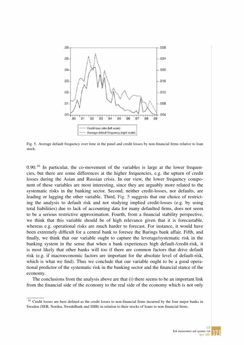
323ECB
Risk measurement and systemic riskApril 2007
Fig. 5. Average default frequency over time in the panel and credit losses by non-financial firms relative to loanstock.
0.90.16 In particular, the co-movement of the variables is large at the lower frequen-cies, but there are some differences at the higher frequencies, e.g. the upturn of creditlosses during the Asian and Russian crisis. In our view, the lower frequency compo-nent of these variables are most interesting, since they are arguably more related to thesystematic risks in the banking sector. Second, neither credit-losses, nor defaults, areleading or lagging the other variable. Third, Fig. 5 suggests that our choice of restrict-ing the analysis to default risk and not studying implied credit-losses (e.g. by usingtotal liabilities) due to lack of accounting data for many defaulted firms, does not seemto be a serious restrictive approximation. Fourth, from a financial stability perspective,we think that this variable should be of high relevance given that it is forecastable,whereas e.g. operational risks are much harder to forecast. For instance, it would havebeen extremely difficult for a central bank to foresee the Barings bank affair. Fifth, andfinally, we think that our variable ought to capture the leverage/systematic risk in thebanking system in the sense that when a bank experiences high default-/credit-risk, itis most likely that other banks will too if there are common factors that drive defaultrisk (e.g. if macroeconomic factors are important for the absolute level of default-risk,which is what we find). Thus we conclude that our variable ought to be a good opera-tional predictor of the systematic risk in the banking sector and the financial stance of theeconomy.
The conclusions from the analysis above are that (i) there seems to be an important linkfrom the financial side of the economy to the real side of the economy which is not only
16 Credit losses are here defined as the credit losses to non-financial firms incurred by the four major banks inSweden (SEB, Nordea, SwedeBank and SHB) in relation to their stocks of loans to non-financial firms.

324ECBRisk measurement and systemic riskApril 2007
statistically, but also quantitatively important and (ii) that the aggregate default rate is agood measure of the financial stance of the economy.
4. The dependency of financial variables on aggregate activity
In this section, we examine if default risk at the firm level is affected by aggregate shocksover and above firm-specific information. Moreover, we will present some brief evidenceof the balance-sheet channel by investigating to what extent standard balance-sheet ratiosare affected by aggregate shocks.
4.1. The default-risk model
In this subsection we present a reduced form statistical model for estimation of probabilityof default for all Swedish incorporated firms. The general idea is to enter factors thatdetermine the probability of default and quantify how these contribute towards predictingdefault realizations. With such estimated probabilities we may proceed to calculate theexpected aggregate default frequency over time.
So far relatively few empirical studies contain a rigorous analysis of the effects frommacro-economic conditions on default behavior and credit risks at the firm level, seee.g. Carling et al. (2004) for a discussion. The logit model of the default probability thatwe present in this subsection includes both idiosyncratic and macroeconomic explanatoryvariables.17 The reason for including aggregate variables in the model is clear by inspectionof Figs. 4 and 5. In Fig. 4, we plot the mean values of the idiosyncratic financial vari-ables that are used in the model 1990Q1–1999Q2. It is obvious that there are no dramaticchanges in the variables during the deep recession 1992–1993. Therefore, a model withonly idiosyncratic variables included is unlikely to fully account for the higher default fre-quency outcomes at the aggregate level depicted in Fig. 2. Therefore, we conjecture that itis important to use aggregate variables in the model.
The macroeconomic variables that we use in the model are the same as included in thedomestic VAR-model given by (1), i.e., the output gap, the domestic annual inflation rate,the REPO rate, and the real exchange rate. A priori, we think that these should have ameasurable impact on the default risk of any given firm. Starting with the output gap, itmay supposedly work as an indicator of demand conditions, i.e., increased demand in theeconomy reducing default risk. Fig. 5 seems, at large, consistent with this view, althoughthere are some spikes in the default rate that presumable have to be attributed to othervariables. Also, it is clear from Fig. 2 that there has been some variation the output gaparound 1996–1998, which has not been met with an increased default rate. Therefore,there must be some other aggregate variables that ought to be important as well. Here, wedecided to include the nominal interest rate (i.e., the REPO rate) because we know that
17 For simplicity, we estimate a logit model rather than a duration model as is done in Carling et al. (2004).Although Carling et al., in contrast with Shumway (2001), found significant evidence of a duration dependence,we believe that this approximation may not be of decisive importance. But an interesting extension of this workis to test for duration dependence in the model.

325ECB
Risk measurement and systemic riskApril 2007
the nominal interest rate was very high during the recession in the beginning of the 1990s,but has came down substantially after the introduction of the inflation target in Sweden.Given the fact that the export to GDP ratio being around 0.40, the real exchange rate isalso a potentially important variable, a deprecation leading to improved competitivenessof Swedish firms. The inflation rate may also be important for firms pricing decisions;higher inflation rates are potentially associated with less certainty about correct relativeprices, and may thus lead to potentially higher default risk. Of course, it also convenientto work with variables that can be generated from the VAR-model in the previous sec-tion. This is the reason why we did not experiment with neither a term structure variable,nor measures of household expectations as in Carling et al. (2004). Finally, as can beseen from Fig. 2, there is a large spike in the REPO rate in the third quarter 1992 due tothe fact that the Riksbank raised the so-called marginal interest rate to 500% in order todefend the fixed exchange rate. If the REPO rate is not adjusted for this exceptional event,the estimation procedure leads to underestimation of the importance of financial costs fordefault behavior. We therefore decided to adjust the REPO rate series in the third quarter of1992.18
In order to highlight how various variables contribute to default risk, we present threemodels in Table 2. One model with accounting ratios only, a second augmented with thedummy variables (PAYDIV, REMARK and TTLFS variables), and finally one with themacroeconomic variables added.19
The results in Table 2 show that both idiosyncratic and aggregate information is impor-tant for explaining default behavior. The variables for omitted (non-reported) financialstatements and remarks on firms payment record are the strongest determinants of defaultin the model. A nice feature of the estimations is that the coefficients for each variable doesnot change substantially when the model is augmented with more variables. In particular, theaccounting ratios in Model I yield roughly the same coefficients as in the complete ModelIII. The predictive power of the accounting data is somewhat less important than the dummyvariables, although the liability-to-assets ratios (TL/TA and TL/TS) and earnings ratios arequite useful.20 The turnover ratio for inventories, liquid asset over total liabilities and the
18 The estimated dummy coefficient in the VAR equals 28.2 in the REPO rate equation. On the basis of this, weadjusted the REPO rate for this quarter to equal 9.8% instead of 38%.19 Since no data on the payment records of firms (i.e., the dummy variables REMARK1 and REMARK2) exist
prior to 1992Q3 for legal storage reasons, the estimation results of Models II and III reported in Table 2 alsoincludes one additional variable (not reported) which is constructed to be an estimate of the average value of thesum of the payment record variables REMARK1 and REMARK2 for the quarters 1990Q1–1992Q2. This variablewas constructed by estimating a logit model for the event of either of the dummy variables REMARK1 andREMARK2 taking on the value 0 or 1 for the period 1992Q3–1999Q2, using all the variables in Model III (exceptREMARK1 and REMARK2 as explanatory variables, of course). The imputed average value for this variable forthe period 1990Q1–1992Q2 (after 1992Q2, it is set to nil) was then constructed as the average estimated probabilityfor each firm and period, i.e., RDt = 1
Nt
∑ipi,t where pi,t denotes the estimated probability for firm i in period
t to have either a REMARK1 or a REMARK2 greater than zero, and Nt denotes the number of firms in period t.The largest gain in including this variable is that the effects of the macroeconomic variables are more accuratelyestimated. For the coefficients of the idiosyncratic variables this variable is of little importance.20 Regarding the importance of the accounting data in the model, we would like to emphasize the following
features. First, firms typically issue annual financial statements, which we transform into quarterly observationsby assuming that they remain the same throughout the reporting period. Given that we define a default event at the

326ECBRisk measurement and systemic riskApril 2007
Table 2Logit estimation results of the default-risk modela
Type of regressor Model I Model II Model III
Coefficient S.E. Coefficient S.E. Coefficient S.E.
Constant −4.76 0.018 −5.22 0.025 −5.88 0.059Idiosyncratic variablesb
EBITDA/TA −1.07 0.022 −1.10 0.028 −1.09 0.046TL/TA 1.07 0.015 0.54 0.020 0.52 0.0233LA/TL −0.10 0.014 −0.15 0.017 −0.16 0.028I/TS 0.27 0.016 0.20 0.021 0.21 0.034TL/TS 0.19 0.004 0.23 0.005 0.22 0.007IP/(IP+EBITDA) 0.09 0.007 0.07 0.009 0.08 0.015PAYDIV −1.91 0.080 −1.85 0.138REMARK 1 1.73 0.032 1.89 0.051REMARK2 2.66 0.020 2.74 0.033TTLFS 3.32 0.019 3.27 0.031Aggregate variablesc
Output gap – yd,t −0.110 0.008Inflation rate – πd,t −0.005 0.009Nominal interest rate – Rd,t 0.072 0.006Real exchange rate – qt −0.006 0.002Summary statisticsd
Mean log-likelihood −0.0669 −0.0491 −0.0484Pseudo R2 0.16 0.37 0.39Aggregate R2 0.26 0.36 0.94Number of observations 2066206 1607049 765263a
a Since we have as many as 7,652,609 quarterly observations, the computer program used to do the MaximumLikelihood estimation of the logit model (GAUSS version 3.5) cannot handle all observations simultaneously. ForModels I and II presented below, we therefore made a random selection of 27 and 21% of the observations suchthat the aggregate default frequency over time is identical to the one computed using all observations. To checkfor convergence in parameter values, we decreased the estimation samples to 26 and 20% of the observations andre-estimated the models. Fortunately, we found convergence in parameter at the three-digit level and the estimationresults in Table 2 are thus based on the 27/21% sized samples, respectively. For Model III this approach was notfeasible because we could not find convergence at the three digit level given the increased number of regressors.For this model, we therefore drew 50 samples of size 10% of the population, and for each parameter we reportthe mean estimate of the resulting 50 sub-sample estimates. The standard errors are based on the mean inverseHessian matrix.
b See Section 2.1 for exact definition of these variables.c See Section 2.2 for definition and sources. The variables are not scaled so the importance of a variable cannot
be interpreted directly from the size of the parameter estimate.d We use Laitila (1993) measure of pseudo R2. The aggregate R2 is computed using all 7,652,609 quarterly
observations.
quarterly frequency, this assumption could presumably lead to underestimation of the importance of the balance-sheet variables in the default risk model. We examined this by estimating the credit-risk model at the annualfrequency instead, and the coefficients for the balance sheets variables were found to be quite similar. In fact, onlythe coefficients for EBITDA/TA and TL/TS were found to be slightly higher (−1.30/0.27 instead of −1.07/0.19,

327ECB
Risk measurement and systemic riskApril 2007
interest coverage ratio appear to be less important. Turning to the macroeconomic variables,we find that they are significant, with the exception of inflation, and have the correct signs.Note that a higher value of the real exchange rate implies a depreciation, and therefore thenegative estimate for this variable suggests that a depreciation on average reduces the riskof default at a given point in time. It should be pointed out that the macroeconomic variablesare highly significant and quantiatively important even if we allow for non-linear effects ofthe balance-sheet variables.21
The advantage of using firm-specific data when estimating the default-risk modelcan be understood as follows. If we estimate Model III without the dummy variables(REMARK1, REMARK2, PAYDIV, and TTLFS are left out because they do not entersignificantly) on aggregate/average data using OLS (TSLS give very similar results), weobtain
dft = −0.23(0.06)
−0.23(0.13)
(EBITDA
TA
)t
+ 0.30(0.06)
(TL
TA
)t
+ 0.09(0.03)
(LA
TL
)t
· · · −0.94(0.21)
(I
TS
)t
+ 0.19(0.08)
(TL
TS
)t
−0.02(0.12)
(IP
IP + EBITDA
)t
· · · − 0.05(0.03)
yd,t −0.05(0.03)
πd,t
+0.12(0.03)
Rd,t +0.002(0.009)
qt + udf,t,
R2 = 0.93, DW = 2.10, Sample : 1990Q1–1999Q2 (T = 38) (3)
If we compare the point estimates in Table 2 with those in (3), we see that they differsubstantially. In particular, the balance-sheet variables I/TS and LA/TL account for a lot ofthe variation in the aggregate default rate, but with the wrong sign. Because the accountingratios are relatively smooth in the aggregate, which is clear from Fig. 4, it is not surprisingthat we obtain spurious results when estimating the model on aggregate data rather than atthe firm level.
In Figs. 6 and 7, we plot the aggregate default rate together with the average predicteddefault rates from Model I (Fig. 6) and Model III (Fig. 7) for the whole sample of firms,i.e., using the 7,652,609 observations. Very interestingly and as conjectured previouslyin the paper, we note in Fig. 6 that the model with firm-specific information only cannotcapture the up- and downturns in average default rate over time, whereas the model withboth micro- and macro-variables included is indeed able to replicate the high default rate
respectively), whereas the other coefficients were actually found to be smaller in the annual model. Moreover,the decision to lag the accounting data 4 quarters in the estimation in order to make the model “operationable”in real-time could presumably also affects the estimated coefficients. Therefore, we re-estimated the model usingcontemporaneous data instead, and again, the estimation results were to found to be very similar.21 When estimating the model where the balance-sheet variables enter in a non-linear way (interaction dummies),
we used the cumulated distributions depicted in Fig. 1 to categorize the balance-sheet variables (three categoriesfor each variable). For instance, we classified EBITDA/TA into the decile-based categories 0–10, 10–90, 90–100,whereas TL/TA was classified into the categories 0–75, 75–90, 90–100. The pseudo R2 in a non-linear version ofModel II is around 0.48, but the aggregate R2 is still slightly below 0.45. So although this model somewhat betteraccount for the aggregate default frequency, macroeconomic variables are still found to be essential for explainingthe absolute level of default risk.

328ECBRisk measurement and systemic riskApril 2007
Fig. 6. Actual and projected default rates at the aggregate level in the estimated default-risk model with onlybalance sheet variables included (Model I).
during the banking crisis, as well as the downturn to very moderate default rates duringthe latter part of the sample. The explained fraction of variation (R2) in the model withmacro-variables included is 94% at the aggregate level, whereas it is as low as 26% inthe model with balance-sheet ratios only.22 This finding is very interesting for severalreasons. First, because it suggests that the high default rates recorded during the bankingcrisis were not exceptional events that we cannot learn anything useful from, but ratherthat they were consequences of unusually bad economic outcomes, both domestically andinternationally.23 Second, when the aggregate default rate is included in the VAR-model
22 The 95% confidence intervals around the fitted values in Figs. 6 and 7 cover the actual values 3/15 numberof times out of the 38 periods. Thus, while Model III outperforms Model I in this respect, it seems as thoughuncertainty around some of the peaks and through is underestimated by the bootstrap procedure that we employand further development is required here. Our single-bootstrap approach for constructing these confidence intervals(bootstrapping parameters in the logit models using a Cholesky-decomposition of the inverse Hessian) seem toresult in underestimation of the confidence intervals. Presumably, by adopting a double-bootstrap procedure onecan account for the uncertainty in estimated standard errors and achieve reasonable coverage for the confidenceintervals. However, a double-bootstrap is currently not feasible in practice.23 Linde (2002) shows that a significant portion of the variation in the domestic macroeconomic variables are of
foreign origin.

329ECB
Risk measurement and systemic riskApril 2007
Fig. 7. Actual and projected default rates at the aggregate level in the estimated default-risk model with macro-variables (Model III).
in Eq. (1) as an endogenous variable, the share of the explained variation in the defaultrate is about 88% and the sum of the two lags for the average default rate is as high as0.74. Without the lags, the share of the explained variation in the average default rateshrinks considerably to about 82%.24 One possible interpretation of these results is thatthe estimated high weight on the lags in the aggregate default rate equation are proxies formissing information at the firm level, since Model III is estimated at the microeconomiclevel and gives a better fit at the aggregate level without any intrinsic dynamics in themodel.
Finally, one way of demonstrating how much is lost by omitting the micro-structure is toregress the average default frequency on the macroeconomic variables included in ModelIII only.
24 Note that the numbers for the aggregate default rate are taken from the VAR estimated on a slightly differentdata sample, 1986Q3–2002Q4. However, when restricting the sample to the same period as used for the default-riskmodel above, the results are actually even more in favor of the micro-model.

330ECBRisk measurement and systemic riskApril 2007
We then obtain
dft = 1.00(0.11)
− 0.19(0.03)
yd,t + 0.04(0.02)
πd,t + 0.02(0.01)
Rd,t − 0.002(0.007)
qt + udf,t,
R2 = 0.65, DW = 1.27, Sample : 1990Q1–1999Q2(T = 38) (4)
If we compare the results of this regression with the results in Table 2, we see that we looseabout 30% of the explanatory power by excluding the balance-sheet variables. This numberis in line with the aggregate R2 reported in Table 2 for Models I and II.
4.2. The dependency of balance-sheet ratios on aggregate shocks
An interesting question is to what extent the balance-sheet ratios are driven by macroe-conomic factors and to what extent they live their own lives, i.e., driven by idiosyncraticshocks. There are good reasons to believe that some of the balance-sheet ratios may be moreindependent of the aggregate state of the economy than others. Consider for example thevariable earnings over total assets (EBITDA/TA). In a favorable macroeconomic situation,earnings should improve, as will total assets. Therefore, the net effect on EBITDA/TA is not
obvious. However, the coverage ratio(
IPIP+EBITDA
), is likely to be more heavily affected by
aggregate shocks, because interest payments on debt (IP) should increase after an increasein the nominal interest rate, while earnings (EBITDA) should fall.
Let Yi,t =[
EBITDA
TAi,t
TL
TAi,t
LA
TLi,t
I
TSi,t
TL
TSi,t
IP
IP + EBITDAIP i,t
]′denote a
6 × 1 vector with the financial ratios for firm i, and let Yt = [Y1,t · · · YNt,t] denote a 6 × Nt
matrix where Nt is the number of firms in the panel in quarter t. Then the process for thefinancial ratios can be written
Yt = ΘYYt−1 + ΘXXt + ut, var(uY,t) = Σu (5)
where Xt is defined by (2). Because we want to estimate the model on quarterly data inorder to better identify the aggregate shocks, but typically have new information aboutthe financial ratios annually, we use annual moving averages when estimating (5). Eachequation in (5) is estimated using the Arellano and Bond (1991) estimator using 1,701,878observations that are constructed from the original data set of all 7,652,609 observations.25
25 Suppose the true model is given by (5). If we define the variables Yt = 14 (Yt + Yt−1 + Yt−2 + Yt−3) and
Xt = 14 (Xt + Xt−1 + Xt−2 + Xt−3), we can write (using (5)):
Yt = ΘYYt−1 + ΘXXt + ut (6)
where ut = 14 (ut + ut−1 + ut−2 + ut−3). This implies that after estimating (6), we can retrieve the parameters of
interest �Y, �X and Σu = 4Σu. As valid instruments (i.e., instruments uncorrelated with the shocks ut) whenestimating (6), we use Yt−5 and Xt−4, thus allowing for one-period, serially correlated measurement errors in Yt.This procedure implies that in order for a firm to be included in the estimation, it must have reported a financialstatement for nine consecutive quarters (3 years). This is why the sample used to estimate (6) is considerablysmaller than the total number of observations.

331ECB
Risk measurement and systemic riskApril 2007
The estimation results of (5) are
ΘY =
⎡⎢⎢⎢⎢⎢⎢⎢⎢⎣
0.807 0.025 −0.0002 −0.029 −0.0003 −0.006
−0.016 0.968 −0.002 0.005 −0.001 0.007
0.007 −0.062 0.938 −0.011 −0.0091 −0.021
−0.004 −0.001 −0.0005 0.940 0.0001 0.002
−0.0007 −0.033 0.005 −0.005 0.990 0.008
−0.031 0.069 −0.005 0.034 0.006 0.573
⎤⎥⎥⎥⎥⎥⎥⎥⎥⎦
,
ΘX = 100 ×
⎡⎢⎢⎢⎢⎢⎢⎢⎢⎣
−0.039 0.060 −0.010 0.031
−0.026 0.016 0.053 0.004
0.187 0.180 −0.089 −0.048
0.033 0.007 0.039 −0.008
−0.524 −0.092 0.154 0.088
−0.167 −0.007 0.148 −0.021
⎤⎥⎥⎥⎥⎥⎥⎥⎥⎦
,
ΣY =
⎡⎢⎢⎢⎢⎢⎢⎢⎢⎣
0.15390 0.02288 −0.22309 0.04976 0.23547 0.37508
0.02288 0.03079 −0.10535 0.01890 0.12979 0.14406
−0.22309 −0.10535 1.35270 −0.18691 −1.04964 −1.45223
0.04976 0.01890 −0.18691 0.07183 0.20798 0.31972
0.23547 0.12979 −1.04964 0.20798 1.24893 1.60151
0.37508 0.14406 −1.45223 0.31972 1.60151 2.78039
⎤⎥⎥⎥⎥⎥⎥⎥⎥⎦
.
We see that there is considerable persistence in the variables, which is presumably dueto the fact that we do not allow for firm or industry specific effects when estimating themodel. The macro-parameters are seemingly small, but the p-values for joint Wald-test ofall the macro-variables are essentially zero in all the equations. However, given the largenumber of observations, this might not come as a big surprise. Arguably more interestingis to examine to what extent aggregate shocks account for variation in the financial ratiosaccording to the estimates. We found that the macro-variables account for maximum 0.1%of the fluctuations in the financial ratios included in Yt, which implies that the accountingratios are essentially are living lives of their own.26 By looking at Fig. 4, these results are not
26 Assuming that the unconditional variance in Xt is unaffected by the variables in Yt in the long-run, which isa reasonable approximation for reasons discussed in Section 3, we can compute the contribution of the macro-variables to fluctuations in Yt as follows. Noting that (5) implies that �Y = �Y�YΘ′
Y +�X�XΘ′X + �u where �Y,
�X and �u are the unconditional covariance matrices for Yt, Xt and ut, respectively. Since the VAR is stable, �X
and �u known (�X is computed as the covariance matrix for the domestic macro-variables 1986Q3–2002Q4 andan estimate of �u is computed from the residuals in (5), we can compute �Y by iterating on this equation, startingwith an arbitrary positive definite matrix as an initial guess. Let Σtot
Y denote the resulting covariance matrix. Theamount of variation due to the idiosyncratic shocks can be found by iterating on �Y = �Y�YΘ′
Y + �u, and we letΣmic
Y denote the resulting covariance matrix. Similarly, the amount of variation in Yt due to aggregate shocks arefound by iterating on �Y = �Y�YΘ′
Y + �X�XΘ′X, and we let Σmac
Y denote the resulting covariance matrix. We can

332ECBRisk measurement and systemic riskApril 2007
that surprising given that the balance-sheet ratios do not display a strong degree of cyclicalbehavior, with the possible exceptions of EBITDA/TA and IP/(IP + EBITDA).
Because the effects of the aggregate shocks were found to be surprisingly low, we alsoconducted the following experiment. For each balance-sheet ratio, we ran simple OLSregressions
Yi,t = c +p∑
s=0
bsXt−p + εi,t,
using both quarterly (setting p = 4) and annual data (using p = 0). From the OLS results, theshare of explained variation in Yi,t due to aggregate shocks is directly given by the R2 forregression i. In none of the estimated equations, we obtained an R2 larger than 0.03, againsuggesting a very minor role for aggregate shocks in explaining the fluctuations in firmsbalance-sheet ratios.
However, before drawing too strong conclusions upon these estimation results. The fol-lowing aspects should be considered. First, the adopted estimation procedure does not allowfor firm specific effects, i.e., there is a common intercept in (5) for all firms. However, whenwe re-estimated allowing for firm-specific effects by including a firm-specific constant, wefound the importance of the aggregate shocks to be at most 1.9% (EBITDA/TA), i.e., verysimilar to the previous results. But surely, the way one models the firm-specific effects canbe of importance for the results. Second, the model is linear, and of course non-linear effectscan be of important. Third, and perhaps most important, is that we do not allow for differentpropagation of aggregate shocks in different industries, since we do not have access to aconsistent industry classification over time for all firms (industry classification was changedin 1992). But it seems unlikely that the basic message conveyed, namely that idiosyncraticrisk is far more important than aggregate shocks, could be overturned.
5. Putting all things together: a simple empirical model of the interaction betweenthe real and the financial economy
In this section, we will briefly describe a simple, but complete model that can be used tostudy the interaction between the real and financial side of the economy. The model consistsof three blocks.
First, we have the VAR-models for the domestic and foreign variables that are estimatedon aggregate data. The domestic VAR(2)-model is given by (1) with the terms
∑2s=1Λs dft−s
added. In order to be able to study the dependency of the foreign variables, we follow Linde(2002) and estimate the following VAR(2)-model for the foreign variables
Zt = Cf + τfTt +2∑
i=1
Bf,iZt−i + uf,t. (7)
then compute the share of fluctuations in the balance sheet ratios due to aggregate shocks as diag (ΣmacY ./Σtot
Y ).Notice that Σmac
Y + ΣmicY = Σtot
Y .

333ECB
Risk measurement and systemic riskApril 2007
The second block of the model is the default-risk model (Model III in Table 2). This model isused to compute the average default frequency that enters into the estimated VAR-model forthe domestic variables, i.e., dft = 1
Nt
∑Nti=1pi,t where pi,t is the estimated default probability
for firm i in period t and Nt is the number of firms in the panel in period t. The third blockof the empirical model is the panel VAR-model (5) for the financial ratios which enter intothe default-risk model. The default-risk model is the crucial link between the “financial”and “real” side of the economy in this empirical model.
6. Policy experiments with the empirical model
In this section, we will discuss how the empirical model can be used to shed light onvarious policy issues. We will show why we think it is useful for policy makers to use micro-information rather than just aggregated data on default risk. That is, we will examine whywe think it is better to include the estimated default-risk model in the empirical model ratherthan making aggregate default frequency an endogenous variable in the VAR-model givenby (1). We will also study how the trade-off regarding stabilizing inflation and the aggregatedefault rate with monetary policy has changed over time in the estimated empirical model.Finally, we will show how one can use the estimated model to compute model consistentjoint forecasts for default-frequency and inflation along with uncertainty bands.
6.1. Computing default frequency distribution percentiles with the model 1991Q1 and1998Q1
In this subsection, we report the results of computing default frequency distributionpercentiles with the estimated empirical model. As initial conditions, we take the portfoliocompositions as they were in 1991Q1 and 1998Q1, respectively, along with correspondingmacroeconomic stances. Note that computing a default frequency distribution is the samething as computing a loss distribution under the assumption that all loans are of the samesize. Computing the default frequency distribution is done in the following way. First wecompute a “trend path” by simulating the economy when no shocks hit the economy, i.e.,ud
t , uft and u
yi,t are all zero and using the actual values on the macro-variables {1990Q4,
1991Q1} and {1997Q4, 1998Q1} as starting values (two lags are used in the VARs). Letdtrendt+h denote the computed trend default rate at horizon h = 1, 2,. . ., 8. Second, we make
an additional simulation using the same initial conditions but this time we allow for shockshitting the economy (i.e., ud
t , uft and u
yi,t are now non-zero). Let dshock
t+h denote the outcomewhen the shocks are included in the model. Third, we compute dDfd
t+h = dshockt+h − dtrend
t+h , whereDfd is spelled out as Default frequency distribution. Fourth, we generate 1000 realizationsof dDfd
t+h and choose the upper (1 − XX/100)th percentile for each horizon h of the simulateddistribution as our Value-at-Risk-measure of the portfolio of firms in the Swedish corporatesector. We also report the (1 − XX/100)th percentile of the distribution for dshock
t+h , to ensurethat the model is consistent with the fact that default risks were higher in the beginning ofthe 1990s than during the boom in late 1990s.27
27 Note that we keep REMARK and TTLFS equal to their initial distributions 1991Q1 and 1998Q1 in thesimulations because we have no model for the dynamics of these variables.

334ECBRisk measurement and systemic riskApril 2007
Table 3Absolute and relative default frequency distribution percentiles at different horizons h into the future using theempirical model 1991Q1 and 1998Q1
Percentile Time period 1991Q1 Time period 1998Q1
h = 1 h = 4 h = 6 h = 8 h = 1 h = 4 h = 6 h = 8
Absolute default frequency percentiles at horizon h (quarters ahead)95 2.02 2.73 2.97 2.78 0.99 0.99 0.99 1.0199 2.17 3.08 3.48 3.46 1.04 1.09 1.06 1.06
Relative default frequency percentiles at horizon h (quarters ahead)95 0.30 0.67 0.85 0.82 0.13 0.18 0.19 0.2099 0.45 1.02 1.36 1.50 0.18 0.28 0.26 0.26
Notes: The absolute default frequency distribution percentiles have been determined from a distribution of 1000outcomes h periods ahead by simulating the empirical model with shocks added to the domestic and foreignVAR-models, and to the VAR-model of the financial ratios. The relative default frequency percentiles have beendetermined from a distribution where a “trend-path” for the default frequency level (given by a simulation of theempirical model where no shocks are added to the economy using the same initial conditions) has been subtractedfrom the absolute default frequency level.
In Table 3, we show the resulting figures for the 1991Q1 portfolio and 1998Q1 port-folio of firms. In the table, the absolute default frequency distribution percentile refersto the (1 − XX/100)th percentile for the dshock
t+h -distribution at horizon h, while the rela-tive default frequency distribution percentile refers to the (1 − XX/100)th percentile for thedDfdt+h-distribution at horizon h. It is important to note that using an aggregate approach, i.e.,
including the aggregate default frequency as an endogenous variable in the VAR-model,would give rise to exactly the same outcome for the (1 − XX/100)th percentile for thedDfdt+h-distribution at horizon h (since the VAR-model is linear). So if these number are dif-
ferent, then this constitutes evidence that the non-linearities induced by the default-riskmodel at the firm level give rise to effects that differ from those in a pure macro-approach.It is harder to say with certainty whether the differences we observe are due to the dif-ferences in portfolio compositions of firms, or differences in the initial macroeconomicconditions.
We learn two things from the results in Table 3. First, the empirical model correctlyidentifies that absolute default risks were substantially higher in 1991 than in 1998. The esti-mated percentiles cover the actual default frequencies during 1991–1992 and 1998–1999,even though the dummy variables REMARK and TTLFS are kept at their initial valuesthroughout the simulations which tends to yield a downward/upward bias for the first/latterperiod. Second, and most importantly, we note that the relative default frequency distri-bution percentiles are at least two times larger for the 1991 portfolio of firms than for the1998 portfolio of firms. This is a clear indication that the micro-data approach using thenon-linear default-risk model differs substantially from a pure macro-approach, because –as mentioned earlier – a pure macro-approach implies that these numbers are the same.
This latter result is quite pronounced, although we have not taken into account in theestimated default-risk model that different industries might display different degrees ofsensitivity to the macroeconomic stance. If this is the case, and if the composition of sharesof firms in different industries has changed over time, then the results reported in Table 3

335ECB
Risk measurement and systemic riskApril 2007
Fig. 8. Impulse response functions to an identified shock to monetary policy in the VAR-model where the defaultrate is endogenous. Solid line shows point estimates and dashed lines 95% confidence interval.
would be even more pronounced, and the evidence in favor of the micro–macro-basedapproach even stronger.
6.2. Is there a trade-off between real and financial stability?
In this subsection, we compute the impulse response functions to an identified monetarypolicy shock, and examine if there is a potential trade-off between stabilizing inflation andoutput and the default frequency. Following Linde (2002), the monetary policy shock isidentified using the so-called recursiveness assumption adopted by Christiano et al. (1999,2005). The assumption being that goods market clear before and financial markets afterthe central bank sets the interest rate. In our empirical model, this implies that output andinflation do not react contemporaneously to a policy shock, whereas the real exchange rateand the default rate do react contemporaneously.
In Fig. 8, we show the impulse response functions to a shock to monetary policy in theestimated VAR-model where the default rate is included as an endogenous variable. Thereare several features worth noting in this graph. According to the VAR, output and inflation

336ECBRisk measurement and systemic riskApril 2007
Fig. 9. Impulse response functions in the estimated VAR-model with the default rate endogenous (point estimates– solid line, dotted lines shows 95% confidence interval) and in the empirical micro–macro-model (dashed line)for 1991Q1.
fall after an increase in the interest rate, whereas the real exchange appreciates.28 As inmany other studies (see e.g. Christiano et al., 2005), the maximum effects are quite delayedin time with peak effects after 1–2 years. Simultaneously, there is a significant and persistentrise in the average default rate. Consequently, the results in Fig. 8 suggest that there is atrade-off between stabilizing the inflation rate and the default rate for monetary policy. Ifthe Riksbank at a given point in time would like to fight inflation more aggressively thanprescribed by the rule normally followed, thereby injecting a positive policy shock (i.e., anunanticipated increase in the REPO rate), this would lead to increasing default frequenciesaccording to the VAR.
However, if we do the same experiment in the empirical micro–macro-model outlinedin Section 4, the picture changes substantially. According to the micro–macro-model, thepotential trade-off between stabilizing the real economy (i.e., output and inflation) and finan-cial stability (approximated by the default rate) is highly time-dependent. In Figs. 9 and 10,
28 Note that the real exchange rate qt is defined as st + pft − pt, implying that a decrease in qt is an appreciation.

337ECB
Risk measurement and systemic riskApril 2007
Fig. 10. Impulse response functions in the estimated VAR-model with the default rate endogenous (point estimates– solid line, dotted lines shows 95% confidence interval) and in the empirical micro–macro-model (dashed line)for 1998Q1.
we plot, for the portfolio of firms in 1991Q1 and 1998Q1, the impulse response func-tions for an identical policy shock as in Fig. 8 along with the impulse response functionsin the estimated VAR-model where the default rate is endogenous.29 As can be seen fromFigs. 9 and 10, the point estimates for output, inflation and the default rate are quite differentin the micro–macro-model compared with the aggregate VAR-approach. For 1991Q1, the
29 The impulse response functions in the micro–macro-model have been computed as follows. As initial condi-tions, we use how the portfolio look like in 1991Q4 and 1998Q1, along with the macroeconomic stance. We thencompute a “trend path” by doing a dynamic simulation of the model when no shocks are hitting the economy, i.e.ud
t , uft and u
yi,t are all zero and we use actual values on the macro-variables {1990Q3, 1990Q4} and {1997Q3,
1997Q4} are used as starting values (two lags are used in the VARs). Let Xtrendt+h
denote the computed trend defaultrate at horizon h = 1,2,. . .,20. Second, we make an additional simulation using exactly the same initial conditionsbut this time we allow for the policy shock hitting the economy (i.e. ud
t is non-zero). Let Xshockt+h
denote the computed
default rate at horizon h = 1,2,. . ., 20 in this case. The impulse responses are then computed as Xshockt+h
− Xtrendt+h
foreach variable in X.

338ECBRisk measurement and systemic riskApril 2007
impulse response functions are roughly the same as in the aggregate VAR-model, althoughthe persistence in the default rate is somewhat lower due to the fact that there is a substantialamount of intrinsic persistence for that variable in the VAR, but none in the default-riskmodel. Turning to 1998Q1, however, we see that the point estimates of the same sized policyshock are rather different in the micro–macro-model compared with the aggregate VAR-model. The effects on the aggregate default frequency are considerably less pronouncedaccording to the micro–macro-model than in the aggregate VAR. Moreover, the differentresponse of the default rate implies that the impulse response functions for output and infla-tion are very different. In the 1998Q1-period, effects on inflation are less than half comparedwith those in the estimated VAR.
Given that the uncertainty about the parameters in the VAR-model (1) is rather high, wecannot claim that the point estimates for the micro–macro-model reported in Figs. 9 and 10are significantly different from the ones in the aggregate VAR in a statistical sense. But ifthe micro–macro-model is a more realistic model than the aggregate VAR-model (we willdiscuss this issue in greater detail the next subsection), then the effects of monetary policyon the economy are state-dependent. This possibility has interesting implications for policyfrom an economic point of view. In this case, monetary policy is a potent tool for stabilizingthe economy in recessions in the sense that small unexpected movements in the interest ratehave relatively large effects on the economy. But in booms, when macroeconomic conditionsare favorable and firms’ balance sheets strong, monetary policy is a less potent tool forstabilizing the economy, i.e., the central bank must inject much larger policy shocks in orderto fight inflation (at the cost of driving up the default frequency). An interesting question,of course, is whether most of these effects come from differences in macroeconomic stancerather than changes in the balance-sheet variables of the firms in the portfolio. Unfortunately,we cannot provide a clear-cut answer to this question. The reason being that the formationof the population of existing firms in a given period is most likely dependent on the stanceof the macroeconomy. Nevertheless, the estimation results for the default-risk Models Iand III suggest that the macroeconomic stance might play a larger role than firms’ balancesheets.
6.3. Joint forecasts of default-frequency and inflation
In this last subsection, we use the micro–macro-model to produce joint forecasts of thedefault-frequency and inflation rate. We use the same initial conditions as in the previ-ous sections and for the same two quarters, 1991Q1 and 1998Q1, i.e., the beginning ofa recession and the beginning of a boom in the economy. To produce these forecasts andassociated uncertainty bands, we perform 1000 dynamic simulations with the estimatedmodel eight quarters into the future. This produces 1000 projections in periods t + 1,. . .,t + 8 for the aggregated default frequency and inflation rate. The resulting forecasts anduncertainty bands are shown in the left-hand panels of Figs. 11 and 12. The right-hand pan-els display corresponding results for the VAR-model (1). The dashed lines are the medianforecasts and the dotted lines represent the 2.5 and 97.5% in the simulated distributions. Thesolid lines show the actual outcomes for 1991Q2–1993Q1 and for 1998Q2–2000Q1. Thereare a couple of interesting features worth noting. First, the micro–macro-model appearsto forecast actual inflation and default frequency quite well, although for the forecasts

339ECB
Risk measurement and systemic riskApril 2007
Fig. 11. Joint dynamic forecasts of the default frequency and inflation eight quarters ahead starting 1991Q1. Theleft panel shows the results for the micro–macro-model, and the right panel the results for the VAR-model wherethe aggregate default rate is included as an endogenous variable. The dashed line is the median forecast, and thedotted lines indicate the 95% confidence interval. The solid line shows the actual outcome.
starting in 1998Q1, actual default frequency is outside the 95% confidence interval in onequarter. It should be noted that since the default risk model is only estimated on data upto 1999Q2, this forecast is to some extent out-of-sample. Second, confirming the resultsreported in Table 3, we see that the uncertainty is much lower in the 1998Q1 forecast.The 95% confidence interval for the predicted default frequency in 1993Q1 is between 1.3and 3.2%, whereas the interval for 2000Q1 is roughly between 0.6 and 1.0%. The con-fidence intervals for VAR-model forecasts are of equal width in both period, suggestingan under-estimation of uncertainty in the first period and an over-estimation in the latterperiod. In comparison with the aggregate VAR-model, the micro–macro-model producea much more plausible picture in that default risk is more severe in the beginning of the1990s, whereas the band width is very tight in the late 1990s, suggesting a very low riskof financial distress. As noted by Christoffersen (1998), this is a desirable property ofa forecasting model. A similar, but less pronounced, interpretation can be done for theinflation rate forecasts. Given an extended data set it would, of course, be very interest-ing to compare the genuine out-of-sample forecasts properties of the micro–macro-model

340ECBRisk measurement and systemic riskApril 2007
Fig. 12. Joint dynamic forecasts of the default frequency and inflation eight quarters ahead starting 1998Q1. Theleft panel shows the results for the micro–macro-model, and the right panel the results for the VAR-model wherethe aggregate default rate is included as an endogenous variable. The dashed line is the median forecast, and thedotted lines indicate the 95% confidence interval. The solid line shows the actual outcome.
and the VAR-model (comparing RMSE and forecasting distributions, see Christoffersen,1998).
7. Conclusions
In this paper, we have studied the interaction between real economic activity and thefinancial stance of the economy using reduced form methods. To this end we have acquireda large panel data set for the Swedish economy during 1990–1999. A period covering abanking crises episode and associated deep recession in the early 1990s, as well as a boomin the latter part of the 1990s.
Our empirical results provide support for the idea that the financial stance of the economymatters for real economic activity. We argue on empirical grounds that the aggregate defaultfrequency is a good proxy for measuring the financial stance, at least this seems to be casefor Sweden. Other financial indicator variables such as stock prices, term structure or the

341ECB
Risk measurement and systemic riskApril 2007
supply loans do not carry information for aggregate quantities and prices, whereas on theother hand housing prices do. We leave for future research to examine the role of housingprices. Moreover, we find that a simple logit model for default at the firm level usingboth firm-specific and macroeconomic variables as explanatory variables can explain theextremely high default frequencies during the banking crisis in the beginning of the 1990s,and also the considerably lower default frequencies in the late 1990s. Furthermore, we findstrong evidence that most of the variation in balance-sheet variables are due to idiosyncraticshocks. Finally, we show that augmenting a standard macroeconomic model with predictedaggregated default-frequencies from the logit model and a simple dynamic panel for thebalance-sheet variables will produce state-dependent effects of monetary policy that arequantitatively important. According to our model, monetary policy is a more potent toolfor stabilizing the economy during recessions than in booms, when the effects of monetarypolicy are rather limited. These latter results provide some implicit empirical support forthe existence of a so-called credit channel of monetary policy.
In our view, the results in the paper suggest that central banks should consider integrationof the analyses of financial stability and economic activity. The empirical micro–macro-model developed in the paper is an example of a simple empirical model, which can be usedfor such a purpose.
The analysis conducted in the paper should be improved and expanded in a variety ofways. First, it would be of interest to examine the out-of-sample forecasting performance ofthe estimated logit model, i.e., whether the estimated model can accurately predict the defaultfrequency rates for the year 2000 and onwards. Another promising research direction is tocondition on firms’ industry-classification, both in the default-risk model and in the dynamicpanel VAR for the balance-sheet variables. Presumably, one reason why the macroeconomicvariables come out as very important in the estimated logit model is that they capturesystematic industry differences in firm-specific variables. Estimating the logit model onindustry data would be a stronger test of whether the empirically important role for themacroeconomic variables is spurious or not. Conditioning on industry would also be anatural way to examine the robustness of the results pertaining to the role of aggregateversus idiosyncratic shocks for the balance-sheet variables. Third, we need to think aboutthe theoretical arguments for macroeconomic factors to enter as separate regressors in thedefault-risk model.
References
Altman, Edward I., 1968. Financial ratios, discriminant analysis and the prediction of corporate bankruptcy. J.Finance XXIII (4), 589–611.
Altman, Edward I., 1971. Railroad bankruptcy propensity. J. Finance XXVI (2), 333–345.Altman, Edward I., 1973. Predicting Railroad bankruptcies in America. Bell J. Econ. 4 (1), 184–211.Altman, Edward I., 1984. The success of business failure prediction models. J. Bank. Finance 4, 171–198.Altman, Edward I., Saunders, Anthony, 1997. Credit risk measurement: developments over the last 20 years. J.
Bank. Finance 21 (11–12), 1721–1742.Arellano, Manuell, Bond, Stephen, 1991. Some Tests of Specification for Panel Data: Monte Carlo Evidence and
an Application to Employment Equations. Rev. Econ. Stud. 58 (2), 277–297.Bernanke, Ben, 1983. Nonmonetary effects of the financial crisis in the propagation mechanism of the Great
Depression. Am. Econ. Rev. 73 (3), 257–276.

342ECBRisk measurement and systemic riskApril 2007
Bernanke, Ben, 1993. Nonmonetary effects of the financial crisis in the propagation mechanism of the GreatDepression. Federal Reserve Bank N Y Quart. Rev. 18 (1), 50–70.
Bernanke, Ben, Gertler, Mark, 1989. Agency costs, net worth and business fluctuations. Am. Econ. Rev. 79 (1),14–31.
Bernanke, Ben, Gertler, Mark, 1990. Financial fragility and economic performance. Quart. J. Econ. 105 (1),87–114.
Bernanke, Ben, Gertler, Mark, 1995. Inside the black box: the credit channel of monetary policy transmission. J.Econ. Perspect. 9 (4), 27–48.
Bernanke, Ben, Gertler, Mark, Gilchrist, Simon, 1996. The financial accelarator and the flight to quality. Rev.Econ. Stat. LXXVIII (1), 1–15.
Calomiris, Charles, Glenn Hubbard, R., 1989. Price flexibility, credit availability and economic fluctuations:evidence from the US, 1894–1909. Quart. J. Econ. 104 (3), 429–452.
Carling, Kenneth, Tor Jacobson, Jesper Linde, and Kasper Roszbach, 2004. ”Corporate Credit Risk Modellingand the Macroeconomy“, manuscript, Sveriges Riksbank.
Christiano, Lawrence J., Eichenbaum, Martin, Charles, L. Evans, 1999. Monetary Policy Shocks: What have WeLearned and to What End Chapter 2. In: John, B. Taylor, Michael, Woodford (Eds.), Handbook of Macroeco-nomics, vol. 1A. Elsevier Science, Amsterdam.
Christiano, Lawrence J., Eichenbaum, Martin, Charles, L. Evans, 2005. Nominal rigidities and the dynamic effectsof a shock to monetary policy. J. Polit. Econ. 113 (1), 1–45.
Christoffersen, Peter F., 1998. Evalutating Interval Forecasts. Int. Econ. Rev. 39 (4), 841–862.Coe, Patrick, 2002. Financial crisis and the Great Depression: a regime switching approach. J. Money Credit
Banking 34 (1), 76–93.Frydman, Halina, Altman, Edward I., Kao, Duen-Li, 1985. Introducing recursive partitioning for financial classi-
fication: the case of financial distress. J. Finance XL (1), 269–291.Gertler, Mark, Gilchrist, Simon, 1993. The role of credit market imperfections in the transmission of monetary
policy: arguments and evidence. Scand. J. Econ. 95 (1), 43–64.Gertler, Mark, Gilchrist, Simon, 1994. Monetary policy, business cycles and the behavior of small manufacturing
firms. Quart. J. Econ. 109, 309–340.Jacobson, Tor, Linde, Jesper, 2000. Credit rating and the business cycle: can bankruptcies be forecast? Sveriges
Riksbank Econ. Rev. 4, 11–33.Laitila, Thomas, 1993. A Pseudo-R2 Measure for Limited and Qualitative Dependent Variable Models. J.
Economet. 56, 341–356.Linde, Jesper, 2002. ”Monetary Policy Shocks and Business Cycle Fluctuations in a Small Open Economy: Sweden
1986–2002, manuscript, Sveriges Riksbank.Lowe, Philip, 2001. Maintaining financial stability: possible policy options. Sveriges Riksbank Econ. Rev. 2001
(2), 25–33.Ludvigson, Sidney, 1998. The channel of monetary transmission to demand: evidence from the market for auto-
mobile credit. J. Money Credit Bank. 30 (3), 365–383.Peek, Joe, Rosengren, Eric, 2000. Collateral damage: effects of the Japanese bank crisis on real activity in the
United States. Am. Econ. Rev. 90 (1), 30–45.Poole, William, 1993. Credit Veils and credit realities. Federal Reserve Bank N Y Quart. Rev. 18 (1), 83–85.Repullo, Rafael, Suarez, Javier, 2000. Entrepreneurial moral hazard and bank monitoring: a model of the credit
channel. Eur. Econ. Rev. 44, 1931–1950.Samolyk, Katherine, 1994. Banking conditions and regional economic performance: evidence of a regional credit
channel. J. Monetary Econ. 34 (2), 259–278.Shumway, Tyler, 2001. Forecasting bankruptcy more accurately: a simple hazard model. J. Business 74 (1),
101–124.

343ECB
Risk measurement and systemic riskApril 2007
1. Introduction
The stability of the financial system, as evidenced by markets that are functioning well,
by key institutions that are operating without major difficulty, and by asset prices that are
not significantly removed from fundamental values, is vital if an economy is to achieve
the objectives of sustained growth and low inflation. A financial system that is stable
will also be resilient and will be able to withstand normal fluctuations in asset prices that
result from dynamic demand and supply conditions, as well as substantial increases in
uncertainty. Financial instability, on the other hand, can impede economic activity and
reduce economic welfare. If financial markets become dysfunctional or the condition of
key institutions becomes severely strained, the attendant pressures on businesses and
households may have adverse effects on the real economy as capital may be prevented
from flowing to worthy investments and credit crunches may develop. To the extent that
those pressures are judged to be sufficiently acute, policymakers may want to respond by
altering the stance of monetary policy. Conversely, economic and monetary policy
surprises can trigger financial instability and compromise the effectiveness of the
The views expressed in this paper are those of the authors and not those of the Board of Governors of the Federal Reserve System. Nelson: [email protected], mail stop 74, Federal Reserve Board, Washington, DC 20551. Perli: [email protected], mail stop 75, Federal Reserve Board, Washington, DC 20551. Andrea Surratt provided excellent research assistance. A previous version of this paper was presented at the Irving Fisher Committee s Workshop on Data Requirements for Analysing the Stability and Vulnerability of Mature Financial Systems, Bank of Canada, Ottawa, June 2005. The authors would like to thank participants to that workshop, as well as several of their Board colleagues, for their comments and suggestions.
SELECTED INDICATORS OF FINANCIAL STABILITY
WILLIAM R. NELSON AND ROBERTO PERLI.
344ECBRisk measurement and systemic riskApril 2007
monetary policy transmission mechanism. As markets react to the new information, large
and sudden price movements may occur that may lead to substantial losses and to
heightened uncertainty and unwillingness to take on risk. Because of the
interdependency between the financial system, the state of the economy, and monetary
policy, monitoring financial markets and appropriately assessing their stability are tasks
of great importance to policymakers. Indeed, the staff of the Federal Reserve Board
devotes a significant amount of time and resources to assess the overall health of the
financial system and, when financial disturbances occur, to judge the implications of
those disturbances for the nonfinancial sector.
The rapid pace of financial innovation that has taken place over the course of the
last decade has brought about a proliferation of new and increasingly sophisticated
financial products, has led to the appearance of new types of institutions, and has created
new and expanded roles for existing institutions. Against this backdrop of increased
complexity, key goals of the Board s staff are to understand financial markets as well as
possible and to be able to identify in a timely fashion the potential consequences of any
new developments. In pursuit of those objectives, the staff relies on its expertise and
judgment, on market intelligence, and on a broad range of financial indicators. Many of
those indicators are measures of financial strength, that is, measures of the ability of
households or businesses to weather shocks without greatly contracting their spending.
Other measures focus on market participants assessments of, and appetite for, risk.
Individual indicators are also combined into aggregate measures that give a synthetic
picture of overall financial conditions and thus summarize the general stability of the
financial system. While notable efforts have been made in the academic literature as well
as at other institutions to develop indicators that could be predictive of adverse
developments, all indicators in use at the Board are contemporaneous in nature and are
used purely as tools to help interpret current conditions.1 And importantly, neither the
1 Reviews and discussions of the predictive ability of various types of indicators, as applied to different
types of crises, are contained, for example, in Berg, A. and Pattillo, C., Are C urrency Crises Predictable? A Test, IM F Staff Papers vol. 46, no. 2, June 1999, and Kumar, M.S. and Persaud, A., Pur e Contagion and Investors Shifting Risk Appetite: Analytical Issues and Empirical Evidence, IMF Working Paper no. 134, 2001.

345ECB
Risk measurement and systemic riskApril 2007
individual nor the aggregate measures are used as black boxes to determ ine policy
actions; rather, they are just a few among a host of instruments that the Board s staff
draws on to inform policy makers of the current state of financial markets.
The individual measures of financial stability used by the Board s staff are taken
from a variety of sources, and are available at a wide range of frequencies. Some, such as
asset prices, are market-based and can be calculated daily, if not even more frequently.
Others, such as financial stocks and flows, are aggregated from individual institutions at a
weekly, monthly, or quarterly basis. Finally, some measures are based on surveys, both
formal and informal, of market participants, and are gathered on an ongoing basis. The
Board of Governors is provided updates about financial market developments often (at
least weekly and sometimes more frequently). The Federal Open Market Committee,
which sets the overnight interbank (federal funds) rate in the United States, is provided
with information on financial conditions before each FOMC meeting, although many
measures are also provided to Committee members on a more frequent basis. Reports on
the functioning of U.S. financial markets are prepared at regular intervals in advance of
international meetings on financial stability. Several Divisions at the Federal Reserve
Board, including the Divisions of Monetary Affairs, Research and Statistics, International
Finance, Bank Supervision and Regulation, and Reserve Bank Operations and Payment
Systems, contribute to the compilation and interpretation of this information.
While the focus of this paper is on quantitative gauges of financial stability, we
should note that qualitative information also figures prominently in the set of tools Board
economists use to assess the state of the financial system. Formal surveys of investors
and bank senior loan officers are conducted regularly and provide timely information on
the respondents views on current developments and their likely future unfolding. More
informal contacts with market participants, either direct or through the Open Market
Desk of the Federal Reserve Bank of New York, are instrumental in the interpretation of
the vast amount of information that is received on any given day. Market contacts are
especially valuable when events are unfolding rapidly and there is no time to wait for
responses to formal surveys. Of course, qualitative information that is received from
346ECBRisk measurement and systemic riskApril 2007
market participants needs to be evaluated, put in context, and possibly filtered, but has
nonetheless repeatedly proved useful in the past.
Sections 2 to 6 of this paper summarize some of the individual and aggregate
indicators that are monitored by the authors and other members of the Board s staff. 2
Section 7 briefly discusses how some of those indicators were used to assess the impact
of the turmoil in the credit markets in the spring of 2005 that was induced by the credit
quality deterioration of two large U.S. automobile manufacturers, and section 8 contains
some conclusive thoughts.
2. Measures based on interest rates and asset prices
Asset prices and interest rates are determined by the supplies and demands of forward-
looking investors and savers; as such, they react nearly instantaneously to investors
judgments about financial conditions. Because many prices and rates are available
virtually instantaneously and continuously, Board staff members monitor a broad range
of them for prompt information on market liquidity and market participants attitudes
toward risk.3
Measures of market liquidity provide information on the ability of financial
markets to absorb large transactions without large changes in prices, and on the premiums
investors are willing to pay to hold more liquid assets. The Board s staff assesses the
liquidity of the market for U.S. Treasury securities, in part, by looking at bid-ask spreads
and volumes. As an example, the top two panels of exhibit 1 plot these measures for the
2 The authors are part of the Monetary and Financial Stability section (MFST) of the Division of Monetary
Affairs (MA). MFST is responsible for analyzing a variety of issues related to financial stability and the operation of financial institutions and markets. Key areas of specialization include the collection and evaluation of information on financial institutions, methods for assessing stress in financial markets, and assisting in the formulation and implementation of policies regarding Reserve Banks’ credit and risk management. Section economists analyze financial developments for the Board of Governors and the FOMC and engage in a broad range of longer-term research projects. Not all the measures discussed in this paper are produced by MFST or MA. 3 This paper draws, in part, from Prag matic Monitoring of Financial Stability, b y William R. Nelson and
Wayne Passmore, in Marrying the Macro- and Micro-Prudential Dimensions of Financial Stability, BIS Papers, No.1, March 2001. That paper contains, among other things, a more detailed description of some of the individual indicators of financial stability in use at the time at the Federal Reserve Board.

347ECB
Risk measurement and systemic riskApril 2007
ten-year on-the-run Treasury security in April and early May, 2005.4 The Treasury
market is an over-the-counter (OTC) market, and consequently bid-ask spreads and
volume data for Treasury securities are more difficult to obtain than for exchange-traded
securities, such as stocks or most futures. The Board s staff currently relies on intraday
data collected by electronic brokers, such as BrokerTec for the interdealer market and
TradeWeb for the dealer-to-customer market. While those electronic brokers do not
represent the whole market, they appear to account for substantial and growing
percentages of the total daily trading volumes in Treasury securities.
[Exhibit 1 about here]
Members of the Board s staff also follow liquidity premiums, defined as the yield
on a less liquid security minus the yield on a highly liquid but otherwise similar security.
Highly liquid securities, generally, can be sold rapidly and at a known price. The amount
investors are willing to pay for that comfort, in the form of higher prices or lower yields
with respect to less liquid securities, may rise rapidly during periods of financial market
difficulties, particularly when the source of such difficulties is heightened investor
uncertainty. Because these spreads may react rapidly to financial difficulties, and are
available at high frequencies, the Board s staff reviews them often. The middle-left panel
of exhibit 1 plots the liquidity premium for the two- and ten-year on-the-run Treasury
securities relative to the corresponding first-off-the-run securities in recent months,
adjusted for the auction cycle. Yield data on Treasury securities are readily available
from a variety of sources.
As suggested by economic theory, expected yields on risky debt instruments and
equities relative to those on riskless assets vary with investors assessments of risk and
willingness to bear risk. The spreads between the yields on riskier and less risky
securities widen when investors judge their relative risks to have increased, and also
4 Corporate credit markets were under stress at that time because of the problems at Ford and General
Motors. The Treasury market, however, was functioning properly, as evidenced by the minimal bid-ask spreads and the substantial volumes.

348ECBRisk measurement and systemic riskApril 2007
when investors demand a higher premium for a given amount of risk. Thus, these
spreads will increase when investor uncertainty increases or financial conditions worsen;
a sharp widening of these spreads has often been a component of financial turmoil.
Examples of such spreads are the differences between investment-grade and speculative-
grade corporate yields and comparable-maturity Treasury yields, plotted in the middle-
right panel of exhibit 1. The Federal Reserve Board receives yields on several thousand
outstanding corporate bonds every day; those data are then used to compute a variety of
indexes, such as those shown in the exhibit. Other spreads over Treasury securities that
are regularly monitored are swap spreads, which can provide information on the credit
quality of the banking sector as well as market liquidity conditions; agency spreads (also
relative to swaps and high-grade corporate debt), which are proxies for the housing
government-sponsored enterprises (or GSEs) cost of funds; and money market spreads,
such as commercial paper spreads (an indicator of the costs of short-term corporate
funding).
Equity prices vary with changes in investors appetite for risk; in investors
expectations for, and uncertainty about, future macroeconomic and firm-specific
outcomes; and in the clarity of information available to investors. To invest in equities,
investors demand a premium over bond yields because the return on bonds is generally
more predictable. The Board s staff assesses the equity premium in a number of ways,
including by comparing the earnings-price ratio of the S&P 500 to the real level of the
ten-year Treasury rate the lower-left panel in exhibit 1. The earnings-price ratio is
calculated using analysts expectations for earnings during the upcoming year and is
adjusted to remove the effect of cyclical changes in earnings. For this purpose, the real
ten-year interest rate is calculated by subtracting a survey-based measure of long-term
inflation expectations from a nominal long-run Treasury rate. Unfortunately, interpreting
changes in this measure of the equity premium is difficult. For example, a decline in the
earnings-price ratio relative to the real interest rate may reflect new economic
information that raises investors expectations of future earnings growth; or it may
indicate that investors have better information or greater certainty about economic
outcomes, or an enhanced appetite for risk. Comparisons of analysts expectations about

349ECB
Risk measurement and systemic riskApril 2007
longer-term earnings growth to the staff s forecast of earnings permit some judgments
about reasons for changes in the earnings-price ratio, but such analysis embodies a great
degree of uncertainty.
The Board s staff uses option prices to measure investors assessment of the likely
volatility of interest rates and equity prices. These measures have proven to be useful and
timely indicators of investor uncertainty and can also be used to construct the probability
distribution of underlying economic outcomes. For example, options on Eurodollar
futures provide a measure of the expected volatility of very short-term rates, which rises
when investors become more uncertain about the future path of near-term monetary
policy (the black line in the lower-right panel of exhibit 1). Equity options (the red line)
provide information on investors uncertainty about equity prices. Those options can also
be used to construct the risk-neutral probability distribution of the returns on underlying
contract (such as the S&P 500 index): A distribution with a long left tail would
presumably indicate elevated market participants concerns about, or aversion to the
possibility of, large losses before the options expiration.
Those described above are but a small sample of the indicators based on interest
rates and asset prices that members of the Board s staff regularly monitor. A rough count
of the number of the basic, individual indicators in daily (or more frequent) production
easily exceeds one hundred. Large amounts of data are necessary to construct those
indicators and use them in daily reports. In addition, the data, which are provided by a
large number of different sources, in different formats, and often at different frequencies,
need to be stored in a convenient and easily-accessible database. Significant resources
are devoted to the maintenance of such a database, in terms of software, storage space,
network accessibility, and personnel.
3. A financial fragility indicator
The information contained in an array of financial variables such as those described
above can be condensed into a financial fragility indicator which estimates the probability
that the U.S. financial system is currently under severe stress. In our view, two episodes

350ECBRisk measurement and systemic riskApril 2007
in recent U.S. financial history can unambiguously be called financial crises the weeks
surrounding the Russian default and the recapitalization of Long Term Capital
Management in the fall of 1998, and the aftermath of September 11, 2001. While the
causes of those crises were entirely different, several key financial variables behaved in a
very similar way during both of those episodes. In particular, risk, liquidity, and term
spreads and implied volatilities all moved significantly higher at those times; moreover,
they did so at a rapid pace and largely at the same time. Based on these observations, the
construction of the indicator follows a two-step process. First, the information contained
in the twelve individual variables listed in the top panel of exhibit 2 is reduced to three
summary statistics that capture their level, their rate of change, and their correlation.5
And second, a logit model is estimated to obtain the probability that, at any given time
and based on the three summary statistics, the behavior of financial markets is analogous
to that of the fall of 1998, and the aftermath of the terrorist attacks of 2001.
[Exhibit 2 about here]
Perhaps the most straightforward summary statistic, plotted in the middle-left
panel, is an arithmetic average of the values of the individual indicators, normalized by
their standard deviations, over the entire sample period from 1994 to the present. As
noted by the gray-shaded regions, the index is quite elevated during times of acute stress.6
As shown in the middle-center panel, the percentage change in the level indicator
computed over rolling eight-week intervals gives a sense of the speed of the movements
in the underlying financial market variables. One might expect that financial markets
would be more fragile during episodes when risk spreads, liquidity premiums, and
volatility indicators are moving sharply higher. Conversely, even when the level of those
indicators remains high, sharp declines in many or all of them might signal the end of a
period of acute financial distress. This rate-of-change indicator again singles out the fall
5 Those indicators are quoted so that higher values would be associated with greater market strains.
6 A third episode during which financial markets where under heavy strain, in addition to the two noted
earlier, was the summer and fall of 2002, when risk spreads widened sharply in response to corporate scandals and credit quality problems at several large institutions.
351ECB
Risk measurement and systemic riskApril 2007
of 1998, the weeks following the terrorist attacks, and the late summer of 2002 as
particularly noteworthy periods.
As shown in the middle-right panel, a time-varying measure of the comovement
in the individual stress variables can be defined as the percentage of the total variation of
the individual variables that can be explained by a single, common factor. This measure
was highest at the time of the global financial crisis of 1998, but the months in the run-up
to Y2K and following the September 11th attacks were also characterized by elevated
correlation among the key financial variables. The shaded region corresponding to the
late summer and fall of 2002 does not stand out as a period of high comovement. Even
though risk spreads widened dramatically at that time, changes in other measures of
market stress were mixed.
The three summary statistics discussed above can be combined into a single
measure of financial fragility and used to model the probability that, at any given time,
the U.S. financial system is in a situation similar to that of the periods identified as crises.
This can be accomplished by fitting a logit model with the three statistics as explanatory
variables and a binary variable which identifies crises on the left-hand-side:
0 1 2 3( )t t t tp L
In the formula above denotes the level indicator, represents the rate-of-change
indicator, and is the comovement indicator.
The model is estimated using weekly data from June 1994 to June 2002, with the
episodes of 1998 and 2001 defined as crises, and then extended out-of-sam ple until the
present.7 The fitted probability of being in a crisis at each date in the sample is shown in
the bottom panel of exhibit 2. As expected, the period of August to October 1998
emerges as the most severe episode of financial fragility in the recent past. The model
does show an increase in the probability of crisis or financial fragility at other points in
time that were not defined as crises. For example, there is a notable uptick in early 1999
7 The summer and fall of 2002 seems to have been, in retrospect, a time of less virulent strain in U.S.
markets, and thus was not classified as a crisis period and was not included in the estimation. A robustness check showed that results would be qualitatively similar if it had been defined as a period of crisis and if the estimation period had been extended to the end of 2002.

352ECBRisk measurement and systemic riskApril 2007
coincident with market concerns about developments in Brazil. The summer and fall of
2002 also stand out, although not at levels as high as the two major crises. The last
notable but m inor peak occurre d in the spring of 2004, when there was some unease
in financial markets about the onset of monetary policy tightening and uncertainty about
the pace at which it would proceed after it was started. The measure has remained at
quite low levels in the spring of 2005, suggesting that the turmoil in credit markets that
was sparked by credit problems at the large automobile manufacturers has not affected
other markets to a significant extent.
4. Mortgage market indicators
In recent years, the U.S. mortgage market has grown rapidly. At the end of 2004, the
total value of mortgages outstanding exceeded $10 trillion, of which $8 trillion were
single-family residential mortgages; of those mortgages, about $4.5 trillion were pooled
into MBS, or mortgage-backed securities. The MBS market is larger than the Treasury
market, the nonfinancial corporate bond market, and the agency market. Virtually all
mortgages pooled into U.S. MBS can be prepaid with no penalty; the prepayment option
induces what is known as negative convexit y, which i mplies that duration decreases
when yields decrease and increases when yields increase. Because of the size of the
market, MBS investors who desire to hedge the prepayment risk of those securities are
now, in the aggregate, required to buy or sell substantial amounts of other financial
instruments; the volumes involved have the potential to reinforce existing market trends.
Such effects can arise under a variety of hedging strategies, but they are perhaps best
understood in a simple example of dynamic hedging. A decline in market interest rates,
say, causes an increase in prepayment risk that reduces the duration of outstanding MBS.
Holders of those securities who wish to maintain the duration of their portfolios at a
constant target would then have to purchase other longer-term fixed-income securities to
add duration, potentially causing yields to fall further. Similar effects tend to amplify
increases in market interest rates as well. Thus, mortgage-related hedging flows have the
potential, at least for a while, to push interest rates significantly above or below the level

353ECB
Risk measurement and systemic riskApril 2007
that would be justified by macroeconomic conditions and expectations, and to increase
the volatility of fixed-income markets. Quantifying the extent to which interest rates may
at times misaligned with economic fundamentals is thus important both from a financial
stability and from a monetary policy perspective.
Several indicators are useful to monitor the impact that mortgage market
conditions have on long-term interest rates. One is the average duration of all fixed-rate
mortgages included in outstanding MBS securities, plotted in the top-left panel of exhibit
3. Periods of time when duration is increasing or decreasing rapidly could be associated
with large hedging flows, as investors buy or sell other fixed-income securities in order to
maintain an approximately constant duration target for their portfolios. A rough estimate
of the size of those flows can be obtained by assuming that investors have a duration
target of 4.5 years and that all MBS investors hedge in the same way.8 The amount of
ten-year equivalent securities that investors would need to hold in their portfolio to
achieve their hypothetical target is plotted in the top-right panel of the exhibit. A rapid
increase or decrease in the amount plotted indicates a corresponding potential increase in
the demand or the supply of ten-year equivalent securities. For example, in July and
early August of 2003, when long-term rates rose rapidly as investors sensed that the
Federal Reserve s easing cycle had ended, up to $2 trillion of ten-year equivalent
securities may have been sold in the market, likely amplifying the upward move in rates
that was already taking place.9
[Exhibit 3 about here]
Perhaps more interesting than duration is convexity (which can be interpreted
roughly as the amount by which duration would change following a 100 basis points
change in yields). MBS convexity depends mostly on how likely mortgage holders are to
prepay their mortgage; that likelihood, in turn, depends on the distance between the
8 The hypothetical 4.5 years target matches the historical average duration of MBS at times when little
refinancing activity was taking place. 9 That estimate is conditional on all mortgage investors fully hedging their portfolios, and as such it
provides an upper limit to the actual flows.

354ECBRisk measurement and systemic riskApril 2007
current mortgage rate and the rates of outstanding mortgages. The middle-left panel of
exhibit 3 shows the percentage of mortgages in outstanding MBS that are economically
refinanceable at a given mortgage rate.10 The steeper the cumulative distribution is at the
current mortgage rate, the higher (more negative) is the convexity of the MBS market. A
time series of convexity itself is plotted at the right; for example, in mid 2005, convexity
was as negative as it had been in recent years, suggesting that the potential risk of
increased volatility in the Treasury and related markets was high.11
The information contained in MBS duration and convexity can be used to
estimate by how much long-term interest rates shocks are likely to be amplified by
mortgage-related hedging flows. Following Perli and Sack (2003), the amplification
factor can be obtained by fitting a GARCH model to the volatility of interest rates, under
the assumption that hedging flows are determined by either the duration, or the
convexity, or the actual amount of refinancing activity currently taking place in the
market.12 The amplification factor is plotted in the last panel of the exhibit: According to
our estimates, up to 20 percent of the downward move in ten-year yields that took place
earlier in 2005 can be attributed to hedging-related flows. While the confidence interval
around that point estimate is fairly wide, it is clear that mortgage hedging could have
significant effects on the fixed-income markets that should be monitored carefully. It is
important to note that hedging activities, at least in our framework, are never the factor
that set off moves in interest rates; they can only amplify, albeit substantially, moves that
are already in place.
10
We assume that the current mortgage rate should be 50 basis points below the existing rate to make it worthwhile to refinance a mortgage due to the various fees associated with extinguishing an old mortgage and starting a new one. The data in the chart are as of the end of May 2005. 11
Duration and convexity help inform judgments of the likelihood that substantial mortgage prepayments will take place. It is also useful to monitor the actual pace of refinancing activity; that measure is shown in the bottom-left panel of exhibit 3. 12
See Perli, R. and Sack, B., Does M ortgage Hedging Amplify Movements in Long-Term Interest Rates?, The Journal of Fixed Income, vol. 13, December 2003, pp. 7-17.

355ECB
Risk measurement and systemic riskApril 2007
5. Measures of conditions of individual institutions
Banks can act as transmission mechanisms of crises because they may sharply contract
credit in response to depositor demands for early and quick redemption of funds. Or,
with deposit insurance, depository institution liabilities may rise with heightened demand
for safety and liquidity. The Federal Reserve collects weekly data on bank credit and the
monetary aggregates which, to some extent, can be used to monitor financial problems.
For example, rapid growth in bank business loans may indicate substitution away from
unreceptive capital markets. Similarly, the monetary aggregates may grow more rapidly
when investors shift funds out of bond and stock mutual funds and into safer and more
liquid bank deposits or money funds.
In the past, both aggressive lending practices and the contraction of lending at
banks have been cited as the transmission mechanism of financial problems to
nonfinancial businesses and households. The Board collects information from
commercial banks four times per year be fore every other FOMC meeting on the
standards and terms on, and demand for, loans to businesses and households in its Senior
Loan Officer Survey on Bank Lending Practices. The Senior Loan Officer Survey poses
a broad range of questions to loan officers at approximately sixty large domestic banks
and twenty-four U.S. branches of foreign banks. On the topic of banks tolerance for
risk, the survey asks about changes in risk premiums on business loans, and about
changes in business loan standards. Although these surveys are not frequent enough to
use for monitoring a quickly unfolding financial crisis, the Federal Reserve has authority
to conduct up to six surveys a year, and has done special surveys when warranted by
financial conditions, most recently in March of 2001.
The Federal Reserve is the umbrella regulator for financial services holding
companies, the primary regulator of bank holding companies, U.S. branches of foreign
banks, and state-chartered banks that are members of the Federal Reserve System; other
institutions have other primary regulators, with whom Federal Reserve regulatory staff
maintains close contacts. Through its supervisory role, the Federal Reserve learns about
the condition and behavior of commercial banks, and acts to maintain the soundness of
these institutions. During periods of financial turmoil, the familiarity with these
356ECBRisk measurement and systemic riskApril 2007
intermediaries deepens the Federal Reserve s understanding of developing conditions.
Communication between the regulatory and policy functions occurs regularly and is
institutionalized at various levels.
Not all financial institutions are depositories; indeed many large ones, such as
insurance companies, the financial subsidiaries of large nonfinancial corporations, the
housing GSEs, etc., are not. In addition, many nonfinancial corporations are heavy
participants in financial markets through their comm ercial paper and bond issuance
programs and often have large lines of cred it with banks. While the Federal Reserve
does not regulate most nondepository financial and nonfinancial institutions, the Board s
staff does monitor information that bears on financial conditions to be able to assess the
impact of difficulties at one or more of those institutions on the financial system. The
monitoring takes place primarily through market-based indicators, such as commercial
paper, corporate bond, and credit default swap (CDS) spreads.
An example of nonfinancial institutions monitoring is presented in the top two
panels of exhibit 4. Two large U.S. automobile manufacturers have experienced some
difficulties in the spring of 2005; the top-left panel of the exhibit plots five-year CDS
spreads for the two institutions, as well as the average spread for CCC-rated institutions.13
While the rating agencies downgraded the obligations of one or both automakers to junk
status beginning in early May, judging from the CDS spreads plotted in the charts market
participants anticipated the rating action by many months. The chart at the top-right
shows the term structure of default probabilities for the two automakers obtained from
CDS spreads as of the end of May 2005. The term structure for another large
nonfinancial institution is shown for comparison purposes.
[Exhibit 4 about here]
The Board s staff monitors CDS on a large number of institutions, both financial
and nonfinancial. As of this writing, CDS data is available on about a thousand U.S.
13
Our data source, Markit, does not report CDS quotes for firms rated below CCC.

357ECB
Risk measurement and systemic riskApril 2007
firms, of which roughly two-thirds are rated investment-grade and the remainder are rated
speculative-grade. With such a large amount of data, it is useful and convenient to
calculate indexes. The investment-grade and speculative-grade indexes computed by
weighting each individual CDS spread by the outstanding liabilities of the corresponding
firm are plotted in the middle panels of exhibit 4. The panels also show the
corresponding market-traded indexes, which are constructed as equally-weighted
averages of the CDS spreads of the component firms. Those indexes can serve as an
alternative to the corporate bond spreads shown in exhibit 1. For several firms CDS are
reported to be more liquid than corporate bonds, so CDS indexes may actually be more
representative of current market conditions than corporate bond spread indexes.14
Credit default swaps give an idea of investors perception of the riskiness of an
institution, but the probabilities of default derived from those instruments are risk-neutral
probabilities, i.e., they incorporate investors attitude toward risk. Obtaining good
measures of actual default probabilities is not easy. One option is to use KMV Corp. s
expected default frequencies (EDF). Those are derived by first computing distances to
default for all publicly traded firms in the U.S. based on Merton s model, and then by
mapping those distances to default into actual defaults using a large historical database.15
Actual default probabilities are typically lower than risk-neutral probabilities since the
latter include a risk premium. Indeed, as shown in the bottom-left panel of exhibit 4, the
EDF for General Motors, as estimated by KMV, has been substantially lower than the
corresponding risk-neutral default probability since 2002; the risk-neutral probability has
surged in March and April of 2005 following the much-publicized problems and the
consequent credit rating downgrades, while the EDF has only edged up. The difference
14
This is especially true at times when individual institutions are experiencing difficulties. At those times many investors would want to sell short the trouble institutions bonds, but those bonds may be hard to obtain in the repo market. Many corporate bonds are typically held by money-managing firms, such as pension funds or mutual funds, that already have plenty of cash and don t need to finance the purchase of the bonds. Those institutions, thus, may not make the bonds available in the repo market, since by doing so they would effectively pay to obtain even more cash. A more detailed analysis of the deviations between CDS and corporate bond spreads is contained in A. Levin, R. Perli, and E. Zakraj e k (2005), The Determinants of Market Frictions in the Corporate Market, manuscript, Federal Reserve Board. 15
For the details see R.C. Merton (1973), A Ratio nal Theory of Option Pricing, Bell Journal of Economics and Management Science, 4, pp. 141 183 and KMV Corp., Modeling Default Risk, Ja nuary 2002, available at www.moodyskmv.com.

358ECBRisk measurement and systemic riskApril 2007
between the two provides a rough estimate of the risk premium that investors demand to
provide credit protection on General Motors obligations.
Before backing up in coincidence with the problems at Ford and General Motors,
credit spreads declined to levels near or below those that prevailed before the crisis of
1998, and some observers have expressed concern that investors are not pricing risk
properly. The difference between risk-neutral probabilities and the EDFs can be taken
for all firms for which data are available, and the average or median of that difference
across all firms is a measure of the corporate risk premium.16 This measure is plotted in
the bottom-right panel of exhibit 4 for both investment-grade and speculative-grade
reference entities. While it is true that the risk premium fell to very low levels (virtually
zero, indeed) in the early part of 2005, it backed up noticeably in March and April,
especially for speculative-grade credits.
6. Probabilities of multiple defaults
Corporate spreads or credit default swap spreads and KMV s EDF can be used to assess
the probability that an individual institution will default within a given time interval.
However, from a systemic risk perspective, the likelihood that more than one institution
will default within a short time period is arguably more interesting than the probability of
an individual default. An estimate of that likelihood can be computed using a
Merton/KMV methodology, modified to take into account the correlation among a group
of financial institutions. According to Merton s work, an institution s probability of
default is a function of three major factors: the market value of the firm s assets (a
measure of the present value of the future free cash flows produced by the firm s assets);
the asset risk, or asset volatility (which measures the uncertainty surrounding the market
value of the firm s assets); and the degree of implied leverage (i.e., the ratio of the book
value of liabilities to the market value of assets). A firm s probability of default
16
See also Berndt, A., Douglas, R., Duffie, D, Ferguson, M., and Schranz, D. (2004), M easuring Default Risk Premia from Default Swap Rates and EDFs, av ailable at www.orie.cornell.edu/aberndt/papers.html. The authors take the ratio of the two probabilities as a measure of the corporate risk premium.

359ECB
Risk measurement and systemic riskApril 2007
increases as the value of assets approaches (from above) the value of liabilities; in theory,
when the two cross, the firm should be assumed to be in default, as future incoming cash
flows will not be sufficient to cover the firm s commitments. At any given time, the
probability of multiple simultaneous defaults can be assessed by simulating the market
value of assets of a number of firms in a certain sample, based on the volatility of those
assets and their correlation. Since market value of assets, asset volatility, and asset
correlation are not directly observable, they first have to be estimated from available
information.
Estimates of the market value of assets and its volatility can be obtained by using
the Black-Scholes methodology and interpreting a firm s market value of equity as a call
option on the firm s asset value struck at the book value of liabilities. The asset
correlation matrix, which is assumed to be time-varying, can be estimated by using
rolling windows or by way of an exponentially-weighted moving average model
(EWMA).
Given current estimates for the market value of assets, asset volatility, and asset
correlation for a sample of firms, the market value of assets of each firm can be simulated
a large number of times for a period of, say, one year, according to a standard Brownian
motion model. The probability of multiple defaults among the institutions in the sample
can be computed as the relative frequency of the event that the market value of assets will
fall below the book value of liabilities for at least two institutions.
That probability, and the probability of at least one default (which is computed
similarly), are plotted in exhibit 5 for a group of about 50 large financial institutions that
includes banks, broker-dealers, and other financial institutions. Over the time period
considered August 1993 to May 2005 the most stressful periods for the institutions in
our sample were, according to those measures, the fall of 1998 and the summer and fall
of 2002. The spring of 2000, when the equity bubble began to burst, also stands out
prominently, although concerns about the viability of financial institutions at that time
appear to have been short-lived. Interestingly, the probabilities of default in the
aftermath of September 11, 2001 were not as high as those in the other periods.
Evidently, while financial markets were under substantial stress, investors did not

360ECBRisk measurement and systemic riskApril 2007
perceive that the solvency of large financial institutions was threatened at the time. The
credit problems at large automobile manufacturers in the spring of 2005 generated only a
minor uptick in both probabilities, indicating that investors perceived those problems as
well contained.
[Exhibit 5 about here]
The probabilities of defaults plotted in exhibit 5 may seem somewhat high, given
that there were relatively few actual defaults of financial institutions since 1994. Several
factors, though, should be taken into account when interpreting those probabilities:
The probability of multiple defaults depends on the sample of institutions that is
considered, and it may well be larger than the probability that any given institution
will default individually. For example, for a sample of 100 firms all independent of
each other and with probability of default of 1 percent within a given time period, the
probability that two or more of them will default within the same period is 26 percent.
For a sample of ten firms, that same probability is just 0.4 percent.
The default probabilities obtained from Merton s model are risk-neutral probabilities,
since it is assumed that the expected return on any firm s asset is the risk-free rate.
Risk-neutral probabilities are typically higher than actual default probabilities, and
possibly much higher at times of intense risk aversion. No attempt is made to
empirically map the risk-neutral default probabilities into actual defaults, as KMV
does.
Actual defaults may not occur as soon as the market value of assets equals the book
value of liabilities; indeed, KMV found empirically that the market value of assets
dips further below that theoretical threshold before a default actually occurs. If a
lower default threshold had been used, the probabilities would have been
correspondingly lower.
These observations suggest that the probabilities shown in exhibit 5 may be most
informative when looked at in relation to their own values at different points in time. For
example, while it could be useful to know that the estimated probability of multiple

361ECB
Risk measurement and systemic riskApril 2007
defaults was about 5 percent after the terrorist attacks of 2001, it may be preferable to
focus on the fact that at that time it was about four times smaller than in the fall of 1998.
7. An example of market monitoring: hedge fund losses
induced by difficulties at Ford and General Motors
News reports surfaced in early May 2005 indicating that some hedge funds may have
incurred significant losses as a result of the widening of corporate credit spreads that
started in mid-March on the heels of the difficulties reported by the two largest U.S.
automobile manufacturers. This section presents some data on hedge fund performance
over that period and describes two of the trades that allegedly resulted in significant
losses. While those trades were quite unprofitable and several funds indeed reported
substantial losses in April and May, the impact on financial markets appears to have been
contained.
Several funds that were mentioned in press reports publicly denied experiencing
particular difficulties. The available data, however, indicate unusually poor hedge fund
returns for the month of April, as shown in the top panel of exhibit 6. Quite a few large
funds reported losses between 5 and 8 percent in that month, and many other smaller
funds performed significantly worse.17
[Exhibit 6 about here]
The known hedge fund losses, and fears of losses as yet unknown, sparked
concerns that some banks and investment banks that have provided prime brokerage
services to hedge funds may have large exposures to troubled funds.18 Most of the major
17
While hedge funds are not required to publish their performance statistics, many voluntarily choose to do so. The source of our data is Bloomberg, which collects data for several thousands hedge funds and funds of hedge funds with a total of more than $800 billion of assets under management. However, the very largest funds, including some of those mentioned in press reports, are not well represented in the database. 18
Prime brokers provide a variety of services to hedge funds, including financing, trade execution, and performance reporting.

362ECBRisk measurement and systemic riskApril 2007
prime brokers stated publicly that most or all of their hedge fund exposures were fully
collateralized and that their capital positions were strong; still, as shown in the bottom
panels, these firms stock prices dropped, and their credit spreads widened notably in mid
May, although from low levels.
While the hedge fund losses that were reported were not dramatic, some of the
funds that did not publicly report their performance may have fared significantly worse.
To better understand the losses that some funds may have suffered as a consequence of
the turmoil in the auto sector, we discuss two types of trades that reportedly were popular
among some funds in the months preceding the roiling of credit markets. One such trade
involved simply selling protection on auto-sector reference entities in the CDS market.
Some funds reportedly believed that Ford and GM spreads already discounted the
possibility of a downgrade to junk back in March, before the actual downgrade and even
before GM warned about poor earnings on March 16. Indeed, both firms CDS spreads
were already comparable to those of low-quality speculative-grade issuers at that time.
GM spreads, however, widened dramatically after its preannouncement and, as shown in
the top panel of exhibit 7, a fund that sold five-year protection on a notional amount of
$10 million of GM debt on March 15 would have sustained a mark-to-market loss of
more than $2 million as of the market close on May 15, or more than 20 percent of the
notional exposure.19 Losses would have been comparable if protection of Ford debt had
been sold instead.20 Hedge funds, of course, could have exited the trade earlier, but they
still would have suffered substantial losses, especially after taking transaction costs into
19
A trade size of $10 million is common among investors. Note that a notional exposure of $10 million does not imply an investment of $10 million: Usually the amount tied up in the trade, as margin or collateral, is much smaller. 20
Hedge funds would have performed marginally better if they had bought a $10 million GM bond, since bond spreads widened a bit less than those on CDS; however, funds would have had to finance the bond purchase. Press reports indicated that some funds may have hedged the CDS position by selling GM stock short or by purchasing equity put options. Given that GM s stock price declined only 8 percent since mid-March, that hedge would have been largely ineffective. For example, investing the entire CDS premium in GM at-the-money put options would have reduced the net loss by less than $0.5 million as of c.o.b. May 15.
363ECB
Risk measurement and systemic riskApril 2007
account.21 Those funds that were willing or able to hold on to their position have seen a
partial reversal of their losses, as GM spreads tightened significantly starting in June.
[Exhibit 7 about here]
A second type of trade that is said to have been popular among hedge funds in the
months leading to the credit market turmoil involved buying and selling protection in
tranches of CDS indexes. Many funds have reportedly sold protection on the equity
tranche of the benchmark investment-grade CDS index, and at the same time bought
protection on an appropriately-scaled notional amount of the mezzanine tranche of the
same index.22 This trade has been dubbed the co rrelation trade because its profitability
depends on investors assessment of the likelihood that defaults among the components
of the index will be clustered in time the def ault correlation.23 As shown in the bottom-
left panel of exhibit 7, spreads on the index equity tranche surged in April and May
especially after Standard and Poor s downgraded Ford s and General Motors debt to
junk status while th ose on the mezzanine tranche rose only moderately. As a
consequence, a correlation trade on a $10 million notional amount entered into on March
15 would have been somewhat profitable until early May the bot tom-right panel but
would have lost between $1 and $2 million after May 7.
21
Bid-ask spreads on Ford and GM CDS reportedly widened in March and April. 22
The index is the average of the spreads of 125 CDS of equal notional amount written on large and liquid reference entities. The equity tranche is designed to absorb the first 3 percent of losses generated by defaults of those reference entities, while the mezzanine tranche absorbs subsequent losses up to 7 percent (further losses are absorbed by more senior tranches). 23
A high default correlation can be interpreted as a sign that investors perceive that the components of the index are vulnerable to systemic shocks. A low default correlation is instead an indication that investors are more concerned about idiosyncratic risk. Default correlation has been low and trending down since the inception of the CDS index in late 2003. The problems and consequent downgrades of Ford and GM evidently exacerbated investors concern about idiosyncratic risk, and default correlation dropped sharply in early May. While the mezzanine tranche is relatively insensitive to changes in default correlation, the value of the equity tranche is directly proportional to it. Intuitively, if defaults are clustered together in time o r highly correlated th e likelihood of a few defaults is lower than if defaults are randomly distributed or uncorrelated. Since a few defaults are all it takes for investors to lose 100 percent of their investment in the equity tranche, the value of that tranche diminishes when default correlation declines.

364ECBRisk measurement and systemic riskApril 2007
The trades examined here were clearly unprofitable, but the magnitude of
actual hedge fund losses depends on several factors, such as the extent of their
involvement in these and similar trades and their degree of leverage. The available data,
including readings from many of the indicators mentioned in this paper and conversations
with market participants, were instrumental in forming the opinion that the situation,
while by no means inconsequential, was not likely to cause major market disruptions and
to spread throughout the financial system. While some strains could obviously be noticed
in the CDS market, where spreads jumped appreciably and index tranches were repriced
sharply, liquidity conditions remained close to normal in most markets throughout the
whole episode, implied volatilities stayed low, there were no signs that markets were
behaving as if a significant crisis was under way, and key financial and nonfinancial
institutions, with the exception of those in the automobile sector, did not show signs of
any particular stress. In the event, a number of hedge funds suffered severe losses, a few
ceased to exist, presumably some prime brokers loans to hedge funds became impaired,
and dealers posted poor trading results that affected their second-quarter profitability.
Overall, however, the financial system proved resilient and absorbed the shock well and
conditions in credit markets returned close to normal by June, with the exception that
implied default correlation remained low; as a consequence, mark-to-market losses
suffered in the correlation trade remain large as of this writing.
8. Conclusions
We have discussed a number of financial indicators that the Board s staff uses as aids in
the interpretation of the conditions of the financial system. Some of those indicators are
simple and readily available, while others are more complex in nature and require access
to substantial amount of data. None are obviously perfect, in the sense that they are
certainly not capable of consistently and correctly gauging the health of financial markets
and institutions at any give time. Moreover, the construction of some of them is not
solidly grounded in economic or financial theory, and as a consequence they perhaps
could be improved. Indeed, all indicators presented here, and certainly their

365ECB
Risk measurement and systemic riskApril 2007
interpretation, are to be considered as wor k in progress. Howeve r, we believe that,
when used in conjunction with staff expertise, solid market intelligence, and good
judgment, they are valuable tools in assessing the state of financial conditions, in pointing
out potential vulnerabilities, and in gauging the severity of crises when they occur.

366ECBRisk measurement and systemic riskApril 2007
Exhibit 1Measures Based on Interest Rates and Asset Prices
Apr. 5 Apr. 12 Apr. 20 Apr. 28 May 5 May 12
0.2
0.3
0.4
0.5
0.6Basis points
Two-year
Ten-year
*Intraday four-hour moving average. Source: BrokerTec.
Interdealer Treasury Bid-Ask Spreads*
4/4 4/7 4/13 4/19 4/25 4/29 5/5 5/112005
100
200
300
400
500$ billion
Interdealer Treasury Volumes*
Weekly average
Two-year
Ten-year
*Source: BrokerTec.
Jan. Feb. Mar. Apr. May2005
0
2
4
6
8
10
12
14
16Basis points
Treasury Liquidity Premiums*
Daily
Two-year
Ten-year
*Computed as the spread of the yield read from an estimated off-the-runyield curve over the on-the-run Treasury yield.
100
110
120
130
140
150
160
Jan. Feb. Mar. Apr. May2005
300
350
400
450
500Basis points Basis pointsCorporate Bond Spreads*
Daily
5-year high-yield(right scale)
10-year BBB(left scale)
*Based on yield curves estimated using Merrill Lynch bond data.
0
2
4
6
8
10
12
1988 1992 1996 2000 2004
E/P ratio
Real long-term Treasury yield*
+
+
* Perpetuity Treasury yield minus Philadelphia Fed 10-year expected inflation.Note. + Denotes the latest observation using daily interest rates and stock prices and latest earnings data from I/B/E/S.
12-Month Forward Trend Earnings-Price Ratio forS&P 500 and Perpetuity Treasury Yield
Monthly
Percent
0
2
4
6
8
10
12
Jan. Feb. Mar. Apr. May2005
8
10
12
14
16
18
20Percent
Implied Volatilities*
Daily
S&P 500 VIX
Eurodollar
*Calculated from options on the underlying contract.

367ECB
Risk measurement and systemic riskApril 2007
Exhibit 2Financial Fragility Indicators
List of Financial Variables Summarized
●
●
●
●
●
●
●
●
●
●
●
●
2-year liquidity premium
10-year liquidity premium
BBB risk spreads
AA risk spreads
High-yield risk spreads (7-year)
3-month Eurodollar confidence interval 1-year ahead
Long bond implied volatility
Eurodollar implied volatility
10-year Treasury implied volatility
SP100 implied volatility (VXO)
Federal funds target - 2-year Treasury
(12-month ahead earnings/SP500) - (10-year Treasury)
1994 1997 2000 2003
100
105
110
115
120
Index of Normalized Variables,January 1994 = 100
Weekly
1994 1997 2000 2003
100
105
110
115
120
1994 1997 2000 2003
-10
0
10
20
30Percent
Rolling Eight-week Changes,Index of Normalized Variables
Weekly
1994 1997 2000 2003
-10
0
10
20
30Percent
1994 1997 2000 2003
30
40
50
60Percent
Comovement Indicator*
Weekly
*Percent of total variation in individual stress variables explained by the first factor in a rolling 26-week window.
1994 1997 2000 2003
30
40
50
60Percent
1994 1995 1996 1997 1998 1999 2000 2001 2002 2003 2004 2005
0.0
0.1
0.2
0.3
0.4
0.5
0.6
0.7
0.8
0.9
1.0ProbabilityFinancial Fragility Indicator (Probability of Crisis)
Weekly

368ECBRisk measurement and systemic riskApril 2007
Exhibit 3Mortgage Market Indicators
Jan. May Sept. Jan. May Sept. Jan. May2003 2004 2005
2.0
2.5
3.0
3.5
4.0
4.5
5.0Years
Mortgage Duration*
Weekly
*Based on a large pool of fixed-rate mortgages included in outstandingmortgage-backed securities. Source: Merrill Lynch.
Jan. May Sept. Jan. May Sept. Jan. May2003 2004 2005
0.0
0.5
1.0
1.5
2.0
2.5
3.0
3.5$ trillion
Amount of 10-Year Equivalent Securities Needed toMaintain a Constant Portfolio Duration*
Weekly
*Staff estimate based on a duration target of 4.5 years.
0
20
40
60
80
100Percent
Thirty-year fixed-rate mortgage rate
Percentage of Economically RefinanceableMortgages*
4 .0 5 .0 6 .0 7 .0 8 .0 9 .0
5.62
*Cumulative percentage of fixed-rate mortgages included in Fannie Mae’s,Freddie Mac’s, and Ginnie Mae’s outstanding MBS that would beeconomically refinanceable for any given mortgage rate. Source: Bloomberg.
Jan. May Sept. Jan. May Sept. Jan. May2003 2004 2005
-2.0
-1.5
-1.0
-0.5
0.0Years
Mortgage Convexity*
Weekly
*Based on a large pool of fixed-rate mortgages included in outstandingmortgage-backed securities. Source: Merrill Lynch.
Jan. May Sept. Jan. May Sept. Jan. May2003 2004 2005
2000
4000
6000
8000
10000
120003/16/90=100
MBA Refinancing Index*
Weekly
*Source: MBA.
Jan. May Sept. Jan. May Sept. Jan. May2003 2004 2005
1.1
1.2
1.3
1.4
1.5
1.6
ConvexityDuration GapRefinancing Index
Amplification of Interest Rate Shocks According toThree Hedging Measures*
Weekly
*Based on Perli and Sack (2003)

369ECB
Risk measurement and systemic riskApril 2007
Exhibit 4Measures of Conditions of Individual Institutions
July Sept. Nov. Jan. Mar. May2004 2005
200
400
600
800
1000
1200Basis points
Credit Default Swap Spreads*
Daily
*Source: Markit.
General Motors
Ford
CCC
B
0
2
4
6
8
10
12
1 3 5 7 10 15 20 30
Percent
0
2
4
6
8
10
12
1 3 5 7 10 15 20 30
Percent
0
2
4
6
8
10
12
1 3 5 7 10 15 20 30
Percent
●
●
●
● ● ● ● ● ●
●
●
●
● ●● ● ● ●
● ● ● ● ● ● ● ● ●
Risk-Neutral Probabilities of Default*
Maturity
General Motors
Ford
Wal-Mart
*As of May 31, 2005. Source: MFST staff calculations.
July Sept. Nov. Jan. Mar. May2004 2005
40
50
60
70
80
90
100Basis points
Investment-grade CDS Indexes*
Daily
*Source: Markit.
Traded
Liability-weighted
July Sept. Nov. Jan. Mar. May2004 2005
200
300
400
500
600Basis points
High-yield CDS Indexes*
Daily
*Source: Markit.
Traded
Liability-weighted
2001 2002 2003 2004
0
2
4
6
8
10Percent
General Motors’ One-year Probabilities of Default*
Monthly
Actual (KMV)
Risk-neutral(from CDS)
*Source: Moody’s KMV and MFST staff calculations.
0
50
100
150
200
250
2001 2002 2003 2004
0
100
200
300
400
500
600
700Basis points Basis points
Corporate Risk Premium*
MonthlySpeculative-grade
(right scale)
Investment-grade(left scale)
*Source: MFST staff calculations.

370ECBRisk measurement and systemic riskApril 2007
Exhibit 5Probabilities of Default of Financial Institutions
1993 1994 1995 1996 1997 1998 1999 2000 2001 2002 2003 2004 2005
0.0
0.1
0.2
0.3
0.4
0.5Probability
Probability of at Least One Default of Financial Institutions*
Weekly
*Probability that at least one out of a group of about 40 large financial institutions will default withinone year. Source: MFST staff calculations.
Jan. May Sept. Jan. May2004 2005
0.02
0.04
0.06
0.08
0.10
0.12
0.14Probability
Weekly
1993 1994 1995 1996 1997 1998 1999 2000 2001 2002 2003 2004 2005
0.00
0.05
0.10
0.15
0.20
0.25
0.30Probability
Probability of Multiple Defaults of Financial Institutions*
Weekly
*Probability that two or more out of a group of about 40 large financial institutions will default withinone year. Source: MFST staff calculations.
Jan. May Sept. Jan. May2004 2005
0.00
0.01
0.02
0.03
0.04Probability
Weekly

371ECB
Risk measurement and systemic riskApril 2007
Exhibit 6Hedge Fund Performance
Mar. Apr. May2005
85
90
95
100
105
110Index: 3/15/05 = 100
Goldman SachsDeutsche BankMerrill LynchJP MorganLehman Bros.
Prime Broker Stock Prices
Ford and GMdowngrades
Mar. Apr. May2005
15
20
25
30
35
40
45
50
55Basis points
Goldman SachsDeutsche BankMerrill LynchJP MorganLehman Bros.
Prime Broker Credit Default Swap Spreads*
Ford and GMdowngrades
*Source: Markit.
0
20
40
60
80
100
# of funds
-4 -3 -2 -1 0 1 2 3 4 moreless
Distribution of Hedge Fund Returns for April 2005*
*Includes only funds with assets in excess of $50 million. Source: Bloomberg.
Percent
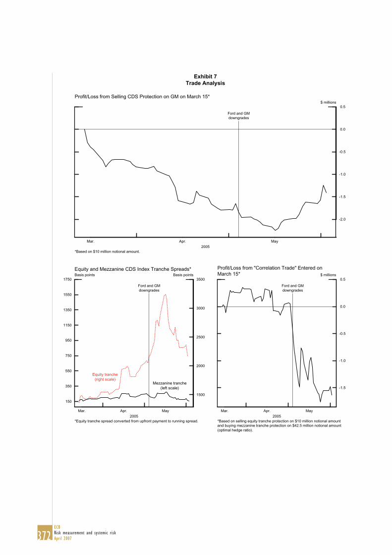
372ECBRisk measurement and systemic riskApril 2007
Exhibit 7Trade Analysis
Mar. Apr. May2005
-2.0
-1.5
-1.0
-0.5
0.0
0.5$ millions
Profit/Loss from Selling CDS Protection on GM on March 15*
Ford and GMdowngrades
*Based on $10 million notional amount.
150
350
550
750
950
1150
1350
1550
1750
Mar. Apr. May2005
1500
2000
2500
3000
3500Basis points Basis pointsEquity and Mezzanine CDS Index Tranche Spreads*
*Equity tranche spread converted from upfront payment to running spread.
Ford and GMdowngrades
Mezzanine tranche(left scale)
Equity tranche(right scale)
Mar. Apr. May2005
-1.5
-1.0
-0.5
0.0
0.5$ millions
Profit/Loss from "Correlation Trade" Entered onMarch 15*
Ford and GMdowngrades
*Based on selling equity tranche protection on $10 million notional amountand buying mezzanine tranche protection on $42.5 million notional amount(optimal hedge ratio).

373ECB
Risk measurement and systemic riskApril 2007
ANNEXES

374ECBRisk measurement and systemic riskApril 2007
programme
In co-operation with theCommittee on the Global Financial System
4th Joint Central Bank Research Conferenceon Risk Measurement and Systemic Risk
Tuesday, 8 to Wednesday, 9 November 2005Frankfurt am Main
1 CONFERENCE PROGRAMME

375ECB
Risk measurement and systemic riskApril 2007
This “Central Bank Research Conference on Risk Measurement and Systemic Risk” is the fourth in a seriesof conferences focusing on issues related to risk measurement and systemic risks from a central bank perspective. It is organised under the auspices of the Committee on the Global Financial System, a Bank forInternational Settlements (BIS)-based Committee of senior central bank officials monitoring financial marketfunctioning for the central bank governors of the G10 countries, and is co-organised by the Bank of Japan,the Federal Reserve Board, the European Central Bank and the CGFS Secretariat. The three earlier conferences were hosted by the Federal Reserve Board, the Bank of Japan, and the BIS in 1995, 1998, and2002, respectively. The conference aims at supporting dialogue among academics, public sector officials,industry professionals involved in trading and risk management as well as central bank staff.

376ECBRisk measurement and systemic riskApril 2007
Tuesday, 8 November 2005
8:00 - 8:30 Registration and Coffee
8:30 - 9:00 Opening Remarks: Otmar Issing (European Central Bank)
9:00 - 10:55 Session I: Non-bank Financial Institutions and Systemic RiskChair: José Viñals (Banco de Espana)
Systemic Risk and Hedge FundsNicholas Chan (Alpha Simplex Group), Mila Getmansky-Sherman1 (University of Massachusetts), Shane Haas (Alpha Simplex Group) and Andrew Lo (Massachusetts Institute of Technology)
Managerial Incentives and Financial ContagionSujit Chakravorti (Federal Reserve Bank of Chicago) and Subir Lall ((International Monetary Fund)
Liquidity Coinsurance, Moral Hazard and Financial ContagionSandro Brusco (State University of New York and University Carlos III) and Fabio Castiglionesi (University Autonoma de Barcelona)
Discussant: Konstantinos E.Tsatsaronis (Bank for International Settlements)
General Discussion
10:55 - 11:15 Coffee
11:15 - 13:10 Session II: Liquidity Risk and ContagionChair: Randall S. Kroszner (University of Chicago)
Illiquidity in the Interbank Payment System Following Wide-Scale DisruptionsMorten L. Bech (Federal Reserve Bank of New York) and Rod Garratt (University of California, Santa Barbara)
Liquidity Risk in Securities SettlementJohan Devriese (National Bank of Belgium) and Janet Mitchell (National Bank of Belgium)
Interbank Contagion: Evidence from Real TransactionsRajkamal Iyer (INSEAD) and José Luis Peydró-Alcalde (European Central Bank)
Discussant: Rafael Repullo (Centro de Estudios Monetarios y Financieros)
General Discussion
13:10 - 14:15 Lunch
14:15 - 16:10 Session III: Credit Risk Transfer and Trading in Credit MarketsChair: Peter Praet (National Bank of Belgium)
Explaining Credit Default Swap Spreads with Equity Volatility and Jump Risks of Individual FirmsBenjamin Yibin Zhang (Moody’s KMV), Hao Zhou (Board of Governors of the Federal Reserve System) and Haibin Zhu (Bank for International Settlements
Insider Trading in Credit DerivativesViral V.Acharya (London Business School) and Timothy Johnson (London Business School)
The Determinants of Market Frictions in the Corporate MarketAndrew Levin (Board of Governors of the Federal Reserve System), Roberto Perli (Board of Governors of the Federal Reserve System) and Egon Zakrajsek (Board of Governors of the Federal Reserve System)
Discussant: Reint Gropp (European Central Ban)
General Discussion
16:10 - 16:30 Coffee
programme
1 The name of the presenter is formatted in bold.

377ECB
Risk measurement and systemic riskApril 2007
16:30 - 18:30 Panel Discussion “The Policy Implications of the Developments in Credit Derivatives and Structured Finance”
Lucas Papademos (European Central Bank, Chair)Sean Kavanagh (Deutsche Bank)Eiji Hirano (Bank of Japan)Michael Alix (Bear Stearns)Roger Ferguson (Board of Governors of the Federal Reserve System)
20:00 Dinner speech: André Icard (Bank for International Settlements)
Wednesday, 9 November 2005
8:45 - 9:00 Coffee
9:00 - 10:55 Session IV: Systemic Risk Across CountriesChair: Fabio Panetta (Banca d’Italia)
Banking System Stability: A Cross-Atlantic PerspectivePhilipp Hartmann (European Central Bank), Stefan Straetmans (Maastricht University) and Casper de Vries (Erasmus University Rotterdam)
Estimating Systemic Risk in the International Financial SystemSöhnke M. Bartram (Lancaster University) Gregory W. Brown (University of North Carolina), and John E. Hund (University of Texas)
A Large Speculator in Contagious Currency Crises: A Single “George Soros” Makes Countries more Vulnerable to Crises, but Mitigates ContagionKenshi Taketa (Bank of Japan)
Discussant: Hans Degryse (Leuven University)
General Discussion
10:55 - 11:15 Coffee
11:15 - 13:10 Session V: Risk Measurement and Market DynamicsChair: Hung Tran (International Monetary Fund)
Bank Credit Risk, Common Factors, and Interdependence of Credit Risk in Money Markets:Observed vs. Fundamental Prices of Bank Credit RiskNaohiko Baba (Bank of Japan) and Shinichi Nishioka (Bank of Japan)
Firm Heterogeneity and Credit Risk DiversificationSamuel Hanson (Federal Reserve Bank of New York), M. Hashem Pesaran (University of Cambridge) and Til Schuermann (Federal Reserve Bank of New York)
Evaluating Value-at-Risk Models with Desk-Level DataJeremy Berkowitz (University of Houston), Peter Christoffersen (McGill University) and Denis Pelletier (North Carolina State University)
Discussant: Joachim Coche (European Central Bank)
General Discussion
13:10 - 14:35 Lunch
14:35 - 16:30 Session VI: Stress Testing and Financial Stability PoliciesChair: Hiroshi Nakaso (Bank of Japan)
Corporate Defaults and Large Macroeconomic ShocksMathias Drehmann (Bank of England), Andrew J. Patton (Bank of England) and Steffen Sorensen (Bank of England)
Exploring Interactions between Real Activity and the Financial StanceTor Jacobson (Sveriges Riksbank), Jesper Lindé (Sveriges Riksbank) and Kasper Roszbach(Sveriges Riksbank)
Selected Indicators of Financial StabilityBill Nelson (Board of Governors of the Federal Reserve System) and Roberto Perli(Board of Governors of the Federal Reserve System)
Discussant: Mark Flannery (University of Florida)
General Discussion
16:30 - 17:00 Concluding Remarks: Lucrezia Reichlin (European Central Bank)
programme

378ECBRisk measurement and systemic riskApril 2007
Fourth Joint Central Bank Research ConferenceList of Participants
Name First name AffiliationAlexopoulou Ioana European Central BankAlix Michael J. Bear, Stearns & Co. IncAlves Ivan European Central BankAngelini Paolo Banca d'ItaliaAsche Henner Deutsche BundesbankAylmer Christopher Bank for International SettlementsBaba Naohiko Bank of JapanBannier Christina Goethe University FrankfurtBartram Söhnke Lancaster UniversityBaudino Patrizia European Central BankBech Morten Linnemann Federal Reserve Bank of New YorkBeck Roland European Central BankBeckmann Rainer Deutsche BundesbankBevilaqua Afonso Central Bank of BrazilBlanz Friedrich Commerzbank AGBraasch Bernd Deutsche BundesbankBreyer Thilo Commerzbank AGBroszeit Timo Austrian Financial Market AuthorityBuck Carsten Landesbank Hessen-ThueringenBurkart Oliver BaFinCase Bradford Federal Reserve BoardCastiglionesi Fabio Universitat Autonoma de BarcelonaChakravorti Sujit Federal Reserve Bank of ChicagoChasiotis Nickolaos University of CologneCheca Nicolas Kissinger McLarty AssociatesChristofferson Peter McGill UniversityCiucci Paolo Bank of ItalyCoche Joachim European Central BankDallmeyer Jens Deutsche Bank AGDe Graeve Ferre Ghent UniversityDegryse Hans Leuven UniversityDevriese Johan National Bank of BelgiumDey Shubhasis Bank of Canadadi Capua Christian Bank of ItalyDiehl Peter HT Finanz KGaA PartnerDötz Niko Deutsche BundesbankDrehmann Mathias Bank of EnglandEbhardt Nicolas Union Investment InstitutionFecht Falko Deutsche BundesbankFehlker Christian European Central BankFell John European Central BankFender Ingo Bank for International SettlementsFerguson Roger Board of Governors of the Federal Reserve SystemFillmann Andreas Haarmann Hemmelrath und PartnerFlannery Mark University of FloridaGehrmann Volker Commerzbank AGGetmansky-Sherman Mila University of Massachusetts
2 LIST OF PARTICIPANTS

379ECB
Risk measurement and systemic riskApril 2007
Giraud Jean-Baptiste CALYON Corporate and Investment BankGrabenweger Johann Universität Wien/ Grabenweger & PartnersGropp Reint European Central BankGutsche Götz Commerzbank AGHabel Martin KfW Banking GroupHaim Yair Bank of IsraelHall Simon Financial Stability Forum Secretariat, BISHartmann Philipp European Central BankHauschild Andreas Deutsche Bank AGHausen Christoph Eurohypo AGHeid Frank Deutsche BundesbankHeider Florian European Central BankHempell Hannah Deutsche BundesbankHerzog Irene-Katharina Herzog SCC: Strategy Consulting & CoachingHirano Eiji Bank of JapanHoffmann Ralf Deutsche Bank AGHryckiewicz Aneta Goethe University FrankfurtIcard André BISIssing Otmar European Central BankIwase Katsuya Commerzbank AGIyer Rajkamal INSEADJohnson Tim London Business SchoolKavanagh Sean Deutsche BankKim Ji-Young The Bank of KoreaKöbel Thomas SEB AGKöhler Horst Commerzbank AGKonz Markus Eurex Clearing AGKress Märten Ministry of FinanceLaganá Marco European Central BankLehmann Hansjörg Swiss National BankLongworth David Bank of CanadaLösler Thomas Deutsche Bank AGLund Melanie Bank of EnglandMai Heike Deutsche Bank AGManganelli Simone European Central BankMarhenke Sven Deutsche Bank AGMayr Bernhard Austrian Financial Market AuthorityMecagni Mauro International Monetary FundMeier Carsten-Patrick Institut für Weltwirtschaft, KielMisina Miroslav Bank of CanadaMitchell Janet National Bank of BelgiumMoerke Wolfgang Deutsche BundesbankMohr Christina IHK FrankfurtMoser Christoph University of MainzNakaso Hiroshi Bank of JapanNyholm Ken European Central Bank
Fourth Joint Central Bank Research ConferenceList of Participants
Name First name Affiliation

380ECBRisk measurement and systemic riskApril 2007
Fourth Joint Central Bank Research ConferenceList of Participants
Name First name AffiliationPanetta Fabio Banca d'ItaliaPapademos Lucas European Central BankPelletier Denis North Carolina State UniversityPeltonen Thomas European Central BankPeretti David Eurohypo AGPerina Martin European Central BankPerli Roberto Federal Reserve BoardPersson Mattias Sveriges RiksbankPesaran Hashem University of CambridgePetrolini Lucia Bank of ItalyPeydró-Alcalde José-Luis European Central BankPraet Peter National Bank of BelgiumQuinten Daniel Deutsche BundesbankReichert Alan Cleveland State UniversityReichlin Lucrezia European Central BankRepullo Rafael CEMFIRetzmann Karl Heinz AKA - Ausfuhrkreditgesellschaft m.b.HRice Tara Federal Reserve Bank of ChicagoRietig Matthias Consulate General of JapanRoeder Carole Banque Centrale du LuxembourgRoger Benoît Société GénéraleRoszbach Kasper Sveriges RiksbankRound James LRP - MainzScheicher Martin European Central BankSchindler Christian BaFinSchindler Alexander Union Asset Management Holding AGSchlecht Christoph BaFinSchmidt-Mohr Udo Deka Investment GmbHSchokker Hubert De Nederlandsche BankSchönewolf Stephanie Commerzbank AGSchulz Alexander Deutsche BundesbankSchwarzkopf Helmut Landesbank Hessen-ThüringenSeidel Thomas Bankhaus Metzler FrankfurtSerifsoy Baris Goethe University FrankfurtShimizu Tokiko Bank of JapanShrieves Ronald University of TennesseeSmets Frank European Central BankSoerensen Bank of EnglandSoramäki Kimmo European Central BankSpeer Nikolas Commerzbank AGSpieker Gabriele KfW Banking GroupStapf Jelena Deutsche BundesbankStolz Stephanie Deutsche Bundesbank
Steffen

381ECB
Risk measurement and systemic riskApril 2007
Taketa Kenshi Bank of JapanTamura Koichi Consulate General of JapanThierfelder Felix Deutsche BundesbankTran Hung International Monetary FundTreacy William Federal Reserve BoardTsatsaronis Kostas Bank for International SettlementsTutyk Vadym IBM Business ConsultingTyrell Marcel Goethe University FrankfurtUhlenbrock Birgit Deutsche BundesbankValentinyiné Marianna Magyar Nemzeti Bank (Central Bank of Hungary)Vanassche Ellen Leuven UniversityVermeir Eric European Central BankVildo Siret Bank of EstoniaViñals Jose Banco de Espanavon Borstel Julia Deutsche Bundesbankvon Köppen-Mertes Isabel European Central Bankvon Thadden Ernst-Ludwig Universität MannheimWalch Karlheinz Deutsche BundesbankWang Qingwei Goethe University FrankfurtWeber Bernhard Greenwich AssociatesWedow Michael Deutsche BundesbankWeissenberger Edgar WWP Financial AdviceWeistroffer Christian Center for Financial StudiesWider Sebastian Deutsche BundesbankWild Harwig Bankhaus Metzler FrankfurtWunderlin Rainer The Bank of New YorkXie Ru Goethe University FrankfurtZakrajsek Egon Federal Reserve BoardFischer Karl-Hermann Goethe University FrankfurtMiloš Ivan Zagreba ka Banka DDSchreiber Jörg Commerzbank AGGündüz Yalin University of KarlsruheSauter Eckhard Landesbank Hessen-Thueringen
Fourth Joint Central Bank Research ConferenceList of Participants
Name First name Affiliation


ISBN 978-928990048-5
9 7 8 9 2 8 9 9 0 0 4 8 5 EURO
PEAN
CEN
TRAL
BAN
KRI
SK M
EASU
REM
ENT
AND
SYS
TEM
IC R
ISK
J
ANU
ARY
2007
RISK MEASUREMENT AND SYSTEMIC RISK
FOURTH JOINTCENTRAL BANK RESEARCHCONFERENCE8-9 NOVEMBER 2005
IN CO-OPERATION WITH THECOMMITTEE ON THE GLOBAL FINANCIAL SYSTEM