THE INFLUENCE OF DEMAND AND CAPITAL CONSTRAINTS

ON SPANISH UNEMPLOYMENT

Javier AndrésCésar Mol iñas

Miguel SebastiánAntonio Zabalza

SGPE-D-88001Enero 1988

IIIIII1II

; i

I

I

I

I

I

1

1

I

I

I

I

I

Este trabajo, elaborado por Javier Andrés, César Molíñas,Miguel Sebastián y Antonio Zabalza, es la ponencia presentada por losautores en la Conferencia del European Une&ployeent Progran celebra-da en Londres los dias 4 y 5 de enero de 1988. El EuropeanUneeployaent Progra» es un proyecto de Investigación en el que parti-cipan Alemania, Austria, Bélgica, Dinamarca, España, Francia, GranBretaña,,Holanda £,Jtal ja,.....<adefflás *de/4rfs ao =ünidoscjdei*»ér1ca,y cuyo objetivo es el estudio de las causas determinantes del desem-pleo. El proyecto está financiado por las Direcciones Generales II(Asuntos Económicos y Financieros) y V (Empleo, Asuntos Sociales,y Educación) de la Comisión de la Comunidad Económica Europea.

IIIII1I

1.

I

I

I

I

I

I

I

I

THE INFLUENCE OF DEMAND AND CAPITAL CONSTRAINTS

. ON SPANISH UNEMPLOYMENT

J. Andres, C. MoHnas, M. Sebastián and A. Zabalza

Introduction

^ This paper reports some preliminary results on the estimation of a| structural model of the Spanish economy, centered around the labour

i and production sectors. Section 2 describes the main facts to beff explained and presents an evaluation of how far the results obtained

; in the paper can help us to understand the recent evolution offt unemployment in Spain. This section, therefore, includes both an* introduction to the problem and a summary of the main findings.I* "Section '3 presents -a brief outline of the7 empirical - model, whichm follows closely the common framework agreed for the project, and

Section 4 presents the results. The final section summarizes the main• conclusions obtained.

2. Main facts and an attempted explanation

2.1 The facts

The main facts under explanation are summarized in Figure 2.1, whichplots the evolution for the last 20 years of the labour force and ofemployment. Until 1974, the increase in the labour force was easilyabsorbed by a corresponding increase in employment. From 1964 to 1974the labour force increased by 10.0 per cent, while employmentincreased by 7.3 per cent. Since then, however, the situation haschanged dramatically. In the last ten years, the labour force has

1IIIIIIIIIIIIIIIIIII

stabilized, with some oscillations, around the level it reached in1974. Employment, on the other hand, has fallen continuously until1985, and only in the last two years shows some signs of recovery. In1974, there were over 13,200 thousand people employed ; by 1985 thisfigure had fallen to under 10,600 thousand. This means thedisappearance of over 2.5 million jobs during the period (almost, a 20per cent fall in employment).

The result of these labour market trends has been a dramatic increasein the rate of unemployment, as can be seen in Figure 2.2. In 1965 theofficial unemployment rate stood at 1.5 per cent of the labour forceand by 1974 it had only increased to 2.6 per cent. By 1985, however,the number of unemployed were almost 3 million, which represented a21.9 per cent of the labour force.

These unprecedented rates have had as a consequence the appearance ofa fairly-large number of long-term unemployed and, therefore, of asubstantial increase in the duration of unemployment. As Figure 2.3shows, in 1964 about 80 per cent of the unemployed population had beenout of job for less than 6 months, and only 10 per cent had beenunemployed for more than one year. In 1985, on the other hand, theformer category represented only a 25 per cent of the total unemployedpopulation, and the latter almost a 58 per cent.l

Things have began to improve in the last two years, with a haltin the decline of employment which so far seems to be holding. In1986 employment increased to 10,820 thousands (a 2.4 per centincrease with respect to 1985) and in 1987 it is expected that itwill reach 11,134 thousands (a 2.9 per cent annual increase).However, since the labour force has also increased substantially,the creation of jobs is not reflected fully in the unemploymentrate, which is expected to only go down to 21.0 per cent in 1987as compared to the 21.9 per cent level it reached in 1985.

IIIIIII

I

II

IIIIIIIIIIII

FIGURE 2.1LABOUR FORCE AND EMPLOYMENT— ( I N LOGS) ~~~~

»_S60

».S2a

».4«a-

».-*67

0. 436

9.40S

9-37*

0.3+3-

9.312-

9-2S1

9.25O-1 1 1 1 11964 1967 197O 1*73

-1 1-—1976

-t 1-

EWPUOTMEKT

LABOUR FORCE

197» 1962 1985

RGURE 2.2UNEMPLOYMENT RATE

.*40

1 1 1—. 1 1 1 1 t > I ') I ' t 1 1 « 1 1 1 I ) »—1*44 IM» t«M 1«*7 1*M 1»M 1»J» It71 IfTS 1>73 ««74 t*7« 1«7« 1*77 1»T» in» «MO IMt 1M1 !«•» !••* 1M4

II1IIIIIIIIIIIIiIIIII

4.

In the second part of this section we attempt an explanation of thesefacts based on the empirical results obtained below. Before discussingthese results, however, it may be interesting to live a brief accountof the evolution of other economic factors which could have had aninfluence on the rise of unemployment and which give a widerperspective to the problem under study.

One such factor is the substantial change that the Spanishoccupational structure has experienced during the last 20 years. Therehas been a big fall of employment in agriculture and a correspondingrise in services, while the share of building and industry hasremained fairly constant (see Figure 2.4). In 1964, agriculturalemployment represented 36 per cent of total employment, while in 1985it had fallen to 16 per cent. On the other hand, employment in theservice sector represented 31 per cent of total employment in 1964,while in 1985 it had risen to almost 50 per cent. This is a majorstructural-change which -has coincided with an-important economiccrisis and which could therefore have had a significant effect onunemployment.

Another factor which could also have influenced unemployment is thereversal in the flow of emigration that took place after the first oilprice shock. Although it is difficult to give precise figures, it hasbeen estimated that in 1973 there were more than 600,000 Spaniardsworking abroad. Since then this figure has decreased substantially. By1978 it had been reduced to 350,000, and it could be even lower now.Again, the coincidence of this inflow of workers with the decline ofthe level of economic activity inside the country, must have meantadded difficulties to absorb the available labour supply.

It is interesting to note that despite this inflow of workers, thelabour force remained fairly constant. This suggests the presence of

IIIIIIIII

• IB

I

I

I

I

I

I

I

I

I

I

I

•o

70

•0

80

ft *0

30-

20-

to-

FIGURE 2.3UNEMPLOYMENT DURATION

1664 1066 10M 1070 1672 1674 1876 1678 «MO 1ft&2 10A4 1866

FIGURE 2.4SECTORIAL EMPLOYMENT

•too

»0

70

•* to

a»-

>»•

SERVICES

CONSTRUCTION

INDUSTRY

12 MONTH

« MOMTH

34 MOMTM

AGRICULTURE

1X4 lt>*« 1»tC lt*7 !•«• tOM 1»7D l»7t l»71 »K7J 1O74 1*76 l»7* 1977 1»7« 117* I0B» t«61 1»*i tMJ

IIIIiIIIIIIIIIIIIIIII

6.

some "discouraged worker" effect, particularly 1-n the height of thecrisis, when the labour force actually declined. The deceleration ofthe labour force that Figure 2.1 shows mus4- be seen in the context ofa participation rate which is the lowest in Europe. In 1984 only a35.6 per cent of the population aged 16 to 65 were in the labourforce. This compares with a 47.8 rate in Great Britain, 43.4 inFrance, 47. 3 Portugal and 41.5 in Italy.

2.2. An attempted explanation

2.2.1 Employment

Figure 2.1 shows that the main reason behind the increase in Spanishunemployment has to do not so much with the evolution of the labourforce, but with the loss of jobs. Therefore, a first thing to do is toinvestigate what could explain the very substantial fall of employmentsince 1974. ' ' " " ,.-..-.,.•-.,,,.,. - -.

We have some results about the proximate causes of this fall, which wetake from an estimated labour demand equation. This equation makesemployment to depend on labour costs, the stock of capital in theeconomy, an index of technical progress, a time trend and an index ofcyclical demand proxied by the degree of capacity utilization (seeAnnex 1).

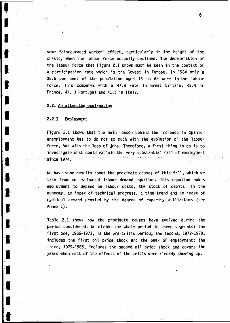
Table 2.1 shows how the proximate causes have evolved during theperiod considered. We divide the whole period in three segments: thefirst one, 1966-1971, is the pre-crisis period; the second, 1972-1978,includes the first oil price shock and the peak of employment; thethird, 1979-1985, includes the second oil price shock and covers theyears when most of the effects of the crisis were already showing up.

IIIIIIIIIIiIIIIIIIIII

7.

Real labour costs, defined as inclusive of Social Securitycontributions and relative to the GDP deflator, have increasedsubstantially in the last 20 years. The average for the period 1972-1978 was 35.1 per cent higher than the average for the period 1966-

Table 2.1

Actual Change of Proximate Determinants of Employment

(percentages)

Real labour costs

Capital stock

Technical progress

Capacity utilization

1966-71/1972-78

35.1

34.3

36.4

1.4

1972-78/1979-85

19.0

20.8

23.5

-5.4

Table 2.2

Contribution of Proximate Determinants to Employment Growth

(percentages)

Real labour costs

Capital stock

Technical progress (plus time)

Capacity utilization

Total change explained

Actual change

1966-71/1972-78

-37.2

52.8

-14.9

0.9

1.6

3.5

1972-78/1979-85

-20.1

32.0

-24.2

-3.2

-15.5

-15.0

IIIIIIIIIIIIIIIIIIIII

8.

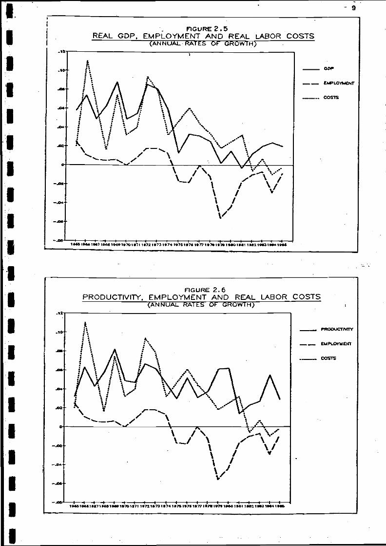
1971. And the average for the period 1979-1985 was 19.0 per centhigher than that for the period 1972-1978. Figures 2.5 and 2.6 showthe annual rate of growth of real labour costs together with that ofemployment, output and productivity. Leaving aside the pro-cyclicalnature of real labour costs, perhaps the most remarkable feature istheir persistent increase during the second half of the seventies inthe face of large falls of employment and very, small rates of outputgrowth. However, there is a distinct deceleration of labour costs inthe last years of the period, which is clearly picked up in Table 2.1.

Figure 2.7 shows the evolution of the stock of capital. There is aclear deceleration in the last ten years, which reflects the smallrates of investment after 1975. Consequently, the rate of growth ofthe stock of capital between the periods 1966-1971 and 1972-1978 is34.3 per cent, while that between 1972-1978 and 1979-1985 is 20.8 percent. Table 1 also shows that technical progress advanced more between-the first two periods~'"(36.4 per cent) than "between-the second andthird (23.5 per cent).

Finally, the index of capital utilization grew by 1.4 per cent betweenthe two periods, and fell by 5.4 per cent between the second andthird. Figure 2.8 plots the level of this variable and the rate ofgrowth of output. The figure illustrates that this is a reasonablevariable to pick up the cycle, and that there is a clear fall indemand after 1975.

As can be seen in Table 2.2, the growth of employment between thefirst two periods is largely explained by the increase in the capitalstock, which more than compensated the negative effect of labour costsand of technical progress. Cyclical demand effects, on the otherhand, were positive but small. The large fall of employment betweenthe second and third periods can be attributed to the smaller growthof the capital stock, which is not sufficient to compensate the

IIIIIIIIIIIIIIIIIIIII

FIGURE 2. 5REAL GDP. EMPLOYMENT AND REAL LABOR COSTS

(ANNUAL RATES 6F GROWTH) :

ODf

_ CMPIOYK4ENT

... COSTS

I I I 1 1 i t I I 1 t I 1 1 1 1 Hl»«6!«*l»«7ie&í 1»*ei»70!»-71 1»721P731»7»1«761»7Í1»771»7S1»761»*CM»«1 1M21««3l«e*1»»S

FIGURE 2.6

PRODUCTIVITY. EMPLOYMENT AND REAL LABOR COSTS(ANNUAL kAT££ OF ÓRÓWTH)

PRODUCTIVITY

EMPLOVtaEMT

COSTS

IIIIIIIIII1IIIIIIIIII

FIGURE 2.7REAL CAPITAL STOCK

(IN LOGS)*-*o

m-sa

m-*e

_2e

•-20

m.12-

a o«-

y.»s-

7.M-

7-BO t « 1- -I- I I « 1- -H1965 1»B7 1M0 1971 1973 1«7S 1»77 1979 1961 1943 IMA

FIGURE 2.8 .CAPACITY UTILIZATION AND RATE OF GROWTH OF GDP

-t-

COP

cu

19BS 19S7 19B9 1971 1973. 1975 1977 1979 1881 19S¿ 19S9

IIIIIIIIIIIIIIIIIIIII

11.

negative effect of labour costs and technical progress, and to thenegative influence of cyclical demand. It is interesting to note thatbetween the last two periods labour costs exerted a smaller negativeinfluence on employment than between the first and second periods.

2.2.2 Unemployment

The analysis so far, although instructive in order to see the effectof labour costs, is unsatisfactory for two reasons: a) because it doesnot take into account factors that may have influenced unemploymentvia labour supply; and b) because it does not say anything about whatdetermines real labour costs and the capital stock.

As we have seen in Figure 2.1, labour supply has been more or lessconstant during the period in which unemployment has increased most.This, however, does not mean that labour supply effects have beenabsent .in '-the determination >of-:• unemployment," as • they --could tiavecompensated one another as far as labour supply is concerned. Also, wehave identified the effect of labour costs on employment, but reallabour costs are endogenous to the model and depend on all factorsthat determine the wages workers desire and the wages employers areprepared to pay.

We have been able to estimate the influence of some of these factorsbut overall the results are somewhat disappointing. Although there arereasons to believe that the changes in the Spanish occupationalstructure described above are relevant, we have been unable toidentify any statistical effect coming from them. Nor has it beenpossible to establish the influence that other factors such as the agestructure of the labour force, degree of mistmatch in the labourmarket, union pressure, firing costs and the replacement ratio mayhave had on the evolution of unemployment. The only wage push factorsthat appear to have a significant statistical effect are Social

IIIIIIIIIIIIIIIIIIIII

12.

Security contributions, indirect taxes and real import prices; thatis, three of the four elements (the fourth being direct taxes) thatform the wedge between real labour costs and the consumption wage.

Another unsatisfactory result of this exercise has been theimpossibility of eliminating the long-run effects of the capital-labour ratio and of technical progress on unemployment. The strongeffect of the capital stock on employment discussed above should intheory be compensated by an equivalent and opposite effect coming fromthe labour force so that there is no long run influence onunemployment. However, we find that the influence of trendproductivity on the desired wage is larger than its influence on thefeasible wage, and this implies the existence of a structural elementof inflationary pressure that can only be neutralized by having moreunemployment.

He feel this -result describes fairly well what has "happened since thefirst oil crisis in the Spanish labour market, but we resist ourselvesto accept it as a permanent feature of wage negotiations in theSpanish economy. As discussed above, labour costs have grownsubstantially in the period 1975 to 1981 despite the existence ofwidespread and rising unemployment (see Figures 2.5 and 2.6). It mustbe remembered that this real wage explosion occurred at a time whenthe previous political regime in Spain was changing into the presentconstitutional monarchy, and that this political transition may havehad a decisive influence on worker's expectations concerning wages. Ifthis is so, the productivity trend -may be picking up part of thetransitory effect that these institutional changes may have had onwages and investors' expectations, and therefore on unemployment. Wehave attempted to introduce this latter effect through a variety ofunion pressure variables, but so far have not been able to detractsignificantly from the strong effect that the trend productivityvariables have on wages.

IIIi

IIIIIIIIIIIIIIIII

13.

Table 2.3 shows the actual changes of the variables determiningdesired and feasible w?ces. We see that there has been a fairly steadyincrease in Social Security contributions (although in the last yearsthey are practically stable), and a moderate fall in indirect taxes(although since 1983 they are rapidly increasing). Real import prices(expressed in pesetas) have gone down by 1.3 per cent between 1966-71and 1972-78, and up by 1.2 per cent between 1972-78 and 1979-85.-Theevolution of technical progress and capacity utilization has alreadybeen described in Table 2.1, and finally we see that the capital-labour ratio has increased substantially throughout the whole period,although, as expected, there is an important deceleration after thefirst oil crisis.

Table 2.4 shows the contribution of these variables to unemployment.Between the first two periods, of the three wage pressure variables,'"Social 'Security contributions' are "the main contributing factor, whileindirect taxes and import prices helped to moderate the rise ofunemployment. However, the main result is the strong effect that theproductivity variables have. They alone would explain over a 100 percent of the rise in unemployment between these two periods. Cyclicaldemand, on the other hand, had only a very weak expansionary effect.Concerning the comparison between the last two periods, we see thatthe effect of Social Security contributions is similar to that of theprevious period, but the moderating influence of indirect taxes ismuch lower and import prices become a contributory factor. The twoproductivity variables continue to exert a large positive effect,which now represents about half of the total change explained.Finally, cyclical demand now becomes contractionary and contributes1.3 points to the rise of unemployment.

1111•

111"

111Ii1W1

1

1

1

1

1

1

\

\

Table 2. 3

Actual Chanqe of Variables Determining Desired(percentages)

1966-71/1972-78

Social Security contributions 4.3

Indirect taxes -1.1

Real import prices* -1.3

Capital-Labour ratio 28.8

Technical progress 36.4

Capacity utilization 1.4

* Weighted by share of imports in GDP.

Table 2. 4

14.

and Feasible Wages

1972-78/1979-85

5.2

- 0.4

1.2

18.5

23.5

-5.4

Explanation of Actual Unemployment ' . ,(percentage points)

1966-71/1972-78

Social Security contributions 3.0

Indirect taxes -2.7

Real import prices* - 1.4

Capital-Labour ratio 4.9

Technical progress 3.6

Capacity utilization -0.3

Total change explained 7. 1

Actual change 3.0

* Weighted by share of imports in GDP

- . _ . . . . _ _

1972-78/1979-85

3.6

-0.9

1.3

3.2

2.4

1-3

10.8

11.9

>

'

•

iIIIIIIII

i

IIIIIIIIIII

15.

We must therefore conclude this part of the analysis with somereserves as to the fundamental causes of the rise of unemployment 1nSpain, due to the fact that the strong effect of the capital-labourratio and of the index of technical progress may be masking theinfluence of other variables. Having said that, the results obtainedsuggest that demand (as proxied by the degree of capacity utilization)had a small part in the explanation of the rise of unemployment afterthe first oil crisis (it explains a 12 per cent of the total change),while Social Security contributions and import prices were significantfactors explaining together more than 45 per cent of the total rise.

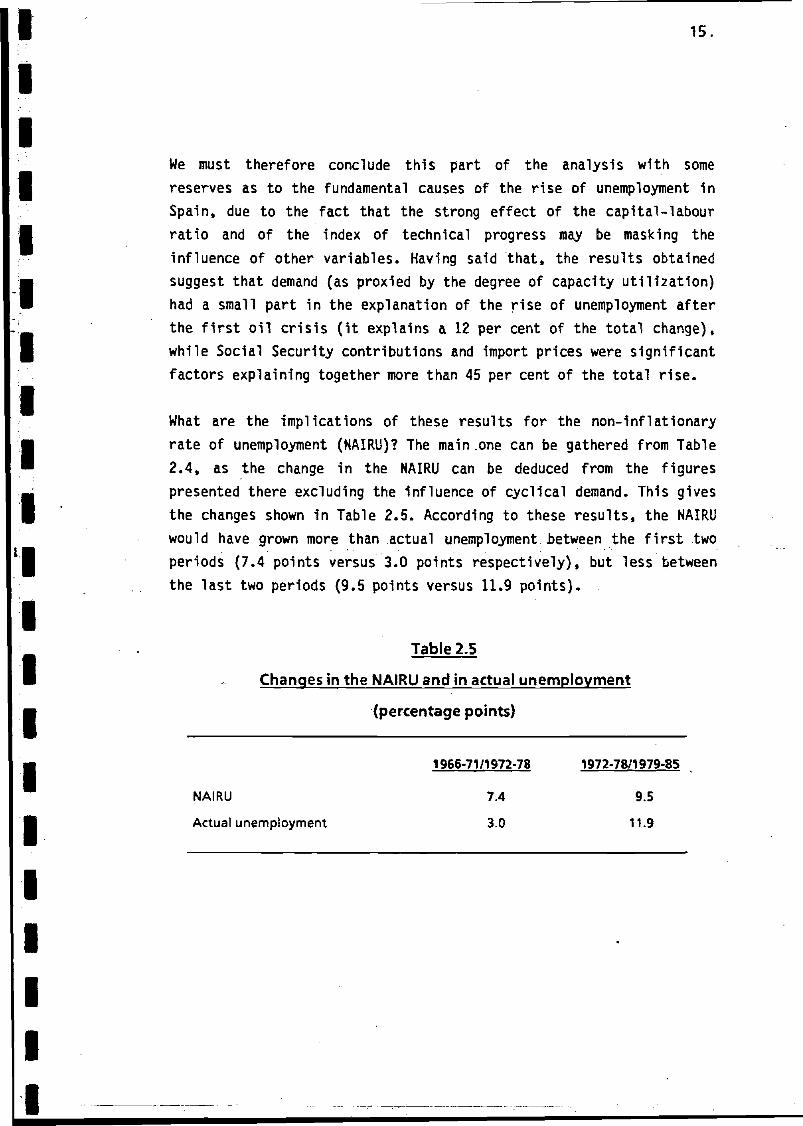
What are the implications of these results for the non-inflationaryrate of unemployment (NAIRU)? The main.one can be gathered from Table2.4, as the change in the NAIRU can be deduced from the figurespresented there excluding the influence of cyclical demand. This givesthe changes shown 1n Table 2.5. According to these results, the NAIRUwould have grown more than actual unemployment between the first twoperiods (7.4 points versus 3.0 points respectively), but less betweenthe last two periods (9.5 points versus 11.9 points).

Table 2.5

Changes in the NAIRU and in actual unemployment

(percentage points)

1966-71/1972-78 1972-78/1979-85

NAIRU 7.4 9.5

Actual unemployment 3.0 11.9

IIIIII

IIIIIIIIIIIIII

16.

Figure 2.9 presents the same information, but showing the level of theNAIRU and its annual evolution.2 We see thav the NAIRU has increasedsubstantially over the whole period and has stayed above or very nearactual unemployment for most of the years. It is only after 1979 thatthe NAIRU begins to relatively slow down its rate of increase, to endin 1985 3.4 points below actual unemployment (18.5 per cent versus21.9 per cent respectively). It must be noted, however, that "theseconclusions are very sensitive to the period used to define theinitial value of the NAIRU. Had this been defined as the average ofactual unemployment for the period 1966-73, then the NAIRU would havebeen below actual unemployment for the whole period, reaching in 1985a level 5.6 points under the actual rate. For this reason, we feelthat the information about changes given in Table 2.5 may be morerelevant than the plots of Figure 2.9.

2.2.3 Demand and capital constraints

In the previous sections we have seen that both cyclical demand andthe capital stock have been relevant factors in the determination ofSpanish unemployment. The stock of capital has played an importantrole in labour demand, and capacity utilization (our proxy forcyclical demand) seems to have had a significant influence on thefeasible wage. Now we want to turn back to these two variables butfrom another perspective.

The stock of capital sets the size of the productive capacity and,therefore, establishes a limit to the amount of workers that could be

It is assumed that the NAIRU of the period 1966-72 coincides withthe average for that period of actual unemployment.

IIiIIII

_12-

FIGURE 2.flU and NAIRU

.1*79

/

—-i——I 1 1 1 \ 1 I t ) 1 1 1 1 1 I f——I 1 11M« »*«7 1»6» 1»(» 1«70 U7Í 1«7Í 1»ZS 1*7* 1»7« t«7« 1«77 1»7« 1«7» 1»«O 1*81 1»»S IM.1 l«8» 1»»5

NAIRU

FIGURE 2.10L, LS, LP and LK

IÍ300+ t

•SO»-1 >

/.

/ \

' .^\.

I/^A-^-CX^ \-^tár Nl_ \\ v

—^ v.

""6 '*•• «»7 18«* ««*• '•»» >«V« 1»72 «7J 197* t»7» t»7« 1»77 I»'» 1»7» lt«O 1M1 1»(« t««3 t»84 IM»

LS

--— LP

IX

IIIIII

IIIIIIIIIIIIII

18-

employed when using fully this capacity. In the long run, withflexible relative prices, this capacity should adjust to accommodatethe available labour supply, but in the short run, a given capitalstock may impose an effective restriction to the amount of workersthat can be employed even in the presence of sufficient demand. It isimportant therefore to find out to what extent unemployment is due toa deficient use of the available capacity, and by how much couldemployment increase if this capacity was fully used. For this purposewe define the concept of "potential employment" as the level ofemployment corresponding to full use of the available capital stock.

As far as demand is concerned, we could be in a situation in whichalthough there is capacity, the level of demand is so small that thereis no incentive for firms to use fully the capital stock available. Inthis situation, aggregate demand sets the effective constraint toemployment. It is therefore instructive to identify also the extent towhich; this circimstance has -been"rrélevant in explatni-ng"• "the~?recent

t evolution of the labour market, and for this purpose we define theconcept of "Keynesian employment" as the level of employment

corresponding to full satisfaction of demand for domestic output.

Figure 2.10 plots the evolution of "potential employment" (LP),"Keynesian employment" (LK), labour supply (LS) and observedemployment (L). Potential employment follows an increasing trend until1975, growing at an annual rate of 0.8 per cent, and then falls almostmonotonically for the rest of the period, at an annual rate of 1.9 percent. This pattern can be explained by the evolution of the optimallabour-capital ratio, given relative factor prices and productionconditions, and by the evolution of the capital stock. Table 2.6 showsthe contribution of these two factors. From 1965 to 1975, the increaseof the capital stock was 49.3 per cent and that of the optimal labour-capital ratio -40.8 per cent, which sums up to the estimated increaseof potential employment of 8.5 per cent. From 1975 to 1985, the

111I•

111,.1

optimal labour-capital stock maintained a similar rate of decline,the capital stock grew much less than in the previous period,being able therefore to absorb the amount of workers freed by thelower requirement of labour per unit of capital.

Table 2.6

Decomposition of the Growth of Potential Employment

(percentages)

1965-1975 1975-1985

Optimal labour-capital ratio -40.8 -40.1

Stock of capital 49.3 22.2

Potential employment 8.5 -17.9

. „ ' . .1*10 - 4ta\sa 4"Kon • i'ltsi'f* &*/fa a+* • •v*fi<a 1 1 w 'OvrvTa-inc "t'f o ~o\/r\T i ft" "i An nf "ttrvt* 01*-iftig nave unen in at wnau i cd i i y c/\p lai nb uuc cvu iu u lun OT puLcr•

employment, is not so much the changes experienced by the factor

19.

butnot

much

itizflmix,

which mantained a uniformly decreasing trend over the whole period,but the much lower rate of increase of the capital stock after 1975.Figure 2.7 above shows this deceleration in the stock of capital, and

1|•

1•

1

1

1

1

1

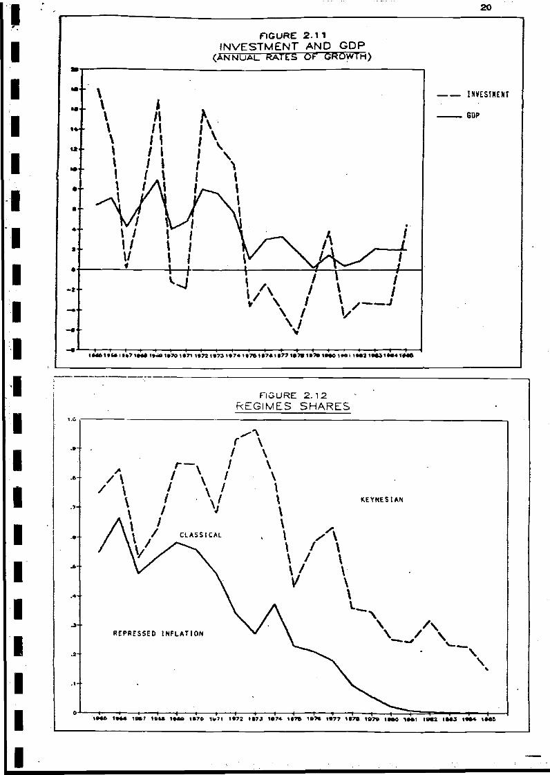
Figure 2.11 the rates of growth of gross capital formation whichessentially the same story.

tell

Keynesian employment follows a similar pattern as potentialemployment, althougt much more cyclical and reaching the peakyears earlier (in 1973). From 1965 to 1973 Keynesian employment

twogrew

at an annual rate of 1.5 per cent, while from 1973 to 1985 it fell atan annual rate of 2.4 per cent. Here again, the evolution of thisof employment depends on two factors: the evolution of demand

typefor

domestic output and the evolution of the labour-output ratio. Table

•

III

20

I

I

I

I

I

I

I

I

I

I

I

I

I

I

I

I

FIGURE 2.1 1INVESTMENT AND GDP

(ANNUAL RATES OF GROWTH)

WESTKENT

GOP

<M»tfMlt»71»M1»«01»701«71 1»73 1«73l»7«1t76l»7«l«T7!»7B1»701»»Ol«M IM2 !••» t *4M 1««S

FIGURE 2.12REGIMES SHARES

-3+

-»H

o->«•? «6U IMA «»70 1H1 1t72 »«7J 1«7* t»7* 1»7« t«77 IÍ7» 1O7» 1MO 1»«t IMZ IMJ 1M4 IM6

I111•

.

111

'• • I H

I•

I-

1

|•

I '.

I

1

1

1

1

21 .

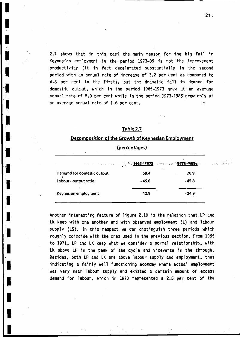
2.7 shows that in this casi the main reason for the big fall inKeynesian employment in the period 1973-85 is not the improvementproductivity (it in fact decelerated substantially in the secondperiod with an annual rate of increase of 3.2 per cent as compared to4.8 per cent in the first), but the dramatic fall in demand fordomestic output, which in the period 1965-1973 grew at an averageannual rate of 5.9 per cent while in the period 1973-1985 grew only atan average annual rate of 1.6 per cent.

Table 2.7

Decomposition of the Growth of Keynesian Employment

(percentages)

• • - . • • . . . . . . - ;H%5-1973 *97J-*S85 ~. . .•: £•'>*-•• " ' ' '"

Demand for domestic output 58.4 20.9*

Labour - output ratio -45.6 -45.8

Keynesian employment 12.8 -24.9

Another interesting feature of Figure 2.10 is the relation that LP andLK keep with one another and with observed employment (L) and laboursupply (IS). In this respect we can distinguish three periods whichroughly coincide with the ones used in the previous section. From 1965

to 1971, LP and LK keep what we consider a normal relationship, withLK above LP in the peak of the cycle and viceversa in the through.Besides, both LP and LK are above labour supply and employment, thusindicating a fairly well functioning economy where actual employmentwas very near labour supply and existed a certain amount of excessdemand for labour, which in 1970 represented a 2.5 per cent of the

IIIIIIIIIIIIIIIIIIIII

22

labour force.3 From 1971 to 1978 the relationship between LP and LK ismore or less maintained, but LP, practically for the whole period,stays below labour supply, which can be interpreted as a signal of theappearance of some limitations as far as the amount of availablecapital is concerned. Also, after the peak of 1973 and towards the endof the period, we observe a clear weakening of Keynesi an demand forlabour, which ends up in 1978 at a level 6.0 per cent below laboursupply.The last period, 1978-1985 is completely different fronv'theother two, and picks up the very strong effects of the crisis uponemployment. Here, LP stays above LK all the years, thus suggestingthat the main constraint to employment growth has been deficientdemand, which by 1985 was requiring a level of employment 21.9 percent below that of labour supply. However, according to our results,demand expansion alone could not have solved this problem as the extraemployment required would very soon have hit the capital constraint.In 1985, without increasing the capital stock, the maximum amount ofemployment would still -have teen 17.7 -per cent below "latnour-supply IT*

The overall conclusion then is that the problem of unemployment inSpain is both a problem of deficient demand and a problem of deficientcapital stock. The second part of this conclusion ties up quite wellwith the results discussed in Section 2.2.1 and presented in Table2.2. The first part, although not inconsistent with the results

3 It should be noted that this situation coexisted with sizeableoutflows of workers to other European countries.

4 Figure 2.12 presents the proportions of firms that are restrictedby demand, by capital or in a situationof repressed inflation(i.e. limited by labour supply) that are implied by-Figure 2.10.

IIIIIIII

Í

II1IIIIIIIIII

23.

presented In Table 2.2, suggests that the magnitude of this effect maybe much larger than what was estimated there.

Naturally, all we have done is to single out demand and capital stockas inmediate constraints limiting the growth of employment, but wehave not as yet managed to explain the factors behind the evolution ofthese two constraints. As far as the capital stock is concerned weneed to investigate what determines investment, and concerning demandwe need to specify in more detail the remaining macro-economicrelationships. Also, we need to do much more work to establish theeffect of relative prices on factor proportions and, hopefully, tounderstand the evolution of prices. The discussion in Section 2.2.2has attempted to go some way 1n that direction, but there are stillmany lacunae to cover. We turn now to the discussion of the empiricalframework and results on which this overall evaluation is based.

IIfiIiIIiiIIIIIIIIIII

24

3. THE ANALYTICAL FRAMEWORK

The model that we estimate in Section 4 is composed ofseven equations arranged in two blocks.

3.1. Wage and Price equations

The wage equation takes the following general form:

(w+t -p) = OQ + 01 (w+ti~p)-i + 012 (B) U + a3A2p + a4x + a5 zl (3-1)

Where o(B) is a polynomial in the backshift operator, w is the grossmonthly wage per employee, p is the value added deflator, tj is theemployer's Social Security contribution rate, U is the unemploymentrate, x an index of trend productivity and Zj is a vector of wagepush factors (it may include, among others, the tax wedge, thereplacement ratio, an index of union pressure, an index of mismatch,-trhe •'age -"Structure -of the'H-abour 'force, -«tcT)'. '5nraTi "letters denotelogarithms but for the tax rates.

Equation (3.1) models the setting of the "target" real wageby wage bargainers. Firms and workers bargain about a real wagetarget that depends on trend productivity, past real wages and a setof wage push factors. Nominal wages are supposed to be set overexpected prices. If actual prices differ over expected prices, realwages will- in the short-run deviate from the level at whichexpectations are fulfilled. This price surprise effect is captured bythe second difference on prices.

The "feasible" real wage is set by firms according to the priceequation which takes the form of a mark up on average labour costs

(p-w-tl) = Po + Pl(p-w-tl)_i + p2(B) w + P3DUK + 04* + P5Z2 (3-2)

III1IIIIII

IIIIII

25

where B(B) is a polynomial 1n B, and B(B)w allows for sluggish nomi-nal adjustment, DUK is the logarithm of the degree of -utilization ofcapital, which stands for a proxy of demand pressure, and Z£ is avector of possible shift factors.

The unemployment rate is the only variable in (3.1) thathas a negative effect on the "target" real wage. Solving for U in thelong-run version of (3.1) and (3.2), setting to zero nominalsurprises and fixing-DUK at its average level, we get the NAIRU,-i.e.the unemployment rate which matches "feasible" and "target" realwages. If equilibrium unemployment is not to be affected by trendproductivity, then 047(1-01) = -837(1-81).

3.2. Short-run employment block

We use a capital-labour relationship similar to that 1n

I - -v 8ean-'¡wid-'tGawosto •J(!Í987). ~ín *a "constant -Teturrrs "to "scale TES "-^-technology, cost minimization leads to a relationship between factor

; proportions and relative factor prices.I

i k -Ip - DO + 01 T(B) WPI + 02 trend (3.3)

where k is the capital stock, Ip is potential employment, 'WPI is theit relative factor price variable, defined as WPI = log (w(l + tjj/cc),™ cc is the user cost of capital and T(B) is a polynomial in B that

•

allows for slow adjustment of the capital-labour ratio to changes 1nrelative prices.

Following Bean and Gavosto (1987), we relate the(unobservable) potential employment Ip to actual employment 1 bymeans of our capacity under-utilization variable (DUK ax - DUK):

Ip = 1 +4.3 (DUKmax - DUK) ; o < <t>3 < 1 (3.4)

1I11•

111•

•

, !

1

iWmt1

i11•

I1•

111

f y26

:

By substituting (3.4) into (3.3) we obtain:

k - 1 =00 + 0! T(B) WPI + 4>3(DUKn,ax - DUK) + o2 trend (3.5)

Then, estimating <j>3 in (3.5), we can compute potentialemployment using (3.4). This gives an estimate of employment at fulluse of productive capacity.

Keynes i an employment is that level of employment that could" -satisfy total demand for domestic output. If demand for domestic

output is large and this generates shortages, these shortages will bemet by lower exports and larger imports. In order to estimate thespillovers of internal demand on exports and imports, we use thefollowing equations:

(X + «h (DUK - (DUKnrfn)) = 60 + «i(X + 4>i(DUK - DUK ))-! + S2(B)WT+• 53W"

IPRXI ' ' • - • • • - . - . / * -3T3 - ',

e

(I - 4>2 (DUK - DUKmin)) =00 + 0! (H>2(DUK - DUKm1n)-i + 62(B)Y ++ 63(8) PRM (3.7)

Where OUKn, is the minimum historical level attained by thedegree of capacity utilization, X is exports, WT is world trade, PRXIis relative export prices, I is imports, Y is real GDP, PRM isrelative import prices, and 62(6), 63(8), 62(8), 63(8) are lagpolynomials. All variables are expressed in logarithms.

Keynes i an output demand YK is the level of demand that theeconomy would face if exports and imports were set to their notionallevel, that is, to X + (DUK - DUKn,1n) and I - 4»2(DUK - DUK,m-n).Then, if Y is observed demand, we have that (in logarithms),

•

Ii

YK = Y + («h SX + $2 Si) (DUK - DUKmin) (3.8)

™ where $x and Sj are the ratios X/Y and I/Y respectively.

| In order to compute the Keynesian labour demand Ik we need arelationship that shows how 1 would adjust in the short-run to

• changes 1n Y. For this purpose we estimate the following: - relationship,

:™ 1 = a0 + ail_i + 32Y + a3K + 34A + 35 trend (3.9)

1 where A is an index of technical progress.

• Then we can transform YK into the Keynesian demand for labour Ikas follows,

i, .- -1* = •*-+ f—^ ' •<*! *K-*-42 &Ó <eüK-4SÜ^^ (3.1fi)

^ Finally, the employment function relates actual employment to| Keynesian and potential labour demand and to labour supply; By

aggregating over micromarkets, some of which are in excess supply and• some of which are in excess demand, we obtain the CES form (see• Lambert 1987)):

I' L = (LK"P + LP~e + LS~P r1/? (3.11)

Iwhere p is the inverse of the imputed mismatch variable that can be

• modelled as

™ f = b0 + bi trend + b2 Z3 (3.12)

II•

I __^_^__

IIIIIIIpIIIIIIIIIIIII

28

where 23 is a vector of mismatch variables that may includestructural change variables, industrial and global mismatch, etc.

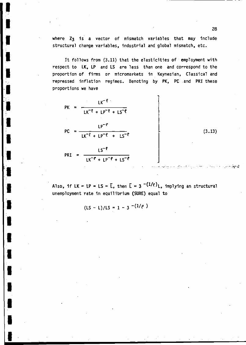
It follows from (3.11) that the elasticities of employment withrespect to LK, LP and LS are less than one and correspond to theproportion of firms or micromarkets in Keynesian, Classical andrepressed inflation regimes. Denoting by PK, PC and PRI theseproportions we have

LK.-ePK =

PC =

LK"f + LP~e + LS~?

LP,-P

LK~f + LP~? + LS~P

LS-fPRI =

LK"f + LP~f + LS~e

(3.13)

Also, if LK = LP = LS = L, then L = 3 'W^L, implying an structuralunemployment rate in equilibrium (SURE) equal to

(LS - L)/LS = 1-3 "Wf )

1IiI

1

....

11''

:

1'..11p111

• 9V

f .•1••1111

29

4. EMPIRICAL RESULTS

The model of Section 3 has been estimated using instrumentalvariables. The wage and price equations have been estimated jointly,and so have been the exports and imports equations.

4.1 Waqe and price equations

Table 4.1 shows the preferred specifications of the wage andprice equations.

The waqe equation is estimated to be static, as no laq of thedependent variable proved significant. Its independent variables tryto capture: (i) the effect of trend productivity on the target wage,(ii) the effect of unemployment, (iii) a nominal surprise er-<?ct, and(iv) shift factors.

(i) Trend productivity effect.••- • • -Trend fHWHirtwity fi$ wíoxisu'tj l . íaEpife'T xjrsstBppTy -> ••-"?* x

ratio KLS. An elasticity close to one could be interpretedas workers trying to claim for wages all observedproductivity gains. The estimate of a unitary elasticity isvery robust both to different specifications of the wageequation and to different specifications of theproductivity variable. Also, the technical progressvariable A has a significant positive effect on wages.

(ii) Unemployment effect.Leaving aside price surprises, the unemployment rate is theonly variable in the wage equation -that can lower thetarget wage. This effect is very significant and' also veryrobust to different specifications. We have tried severallags of U, its logarithm, first and second differences,long term unemployment, and male unemployment as different

•

11i•

ii1Vi. t ' -'

I:

.lm

1

1

i'fli

1f •

i•••1'

1111111

\30

\measures of labor market tightness. Neither of themImproves the results shown in Table 4.1.

(iii) Nominal surprises.Nominal surprise, as measured by the second difference ofp, exert, as expected, a significant negative effect onreal wages.

(iv) Wage pressure effects.We have tried unsuccessfully a variety of shift ~vari abrí essuch as replacement ratios, mismatch, union power proxies,benefit proxies and age structure of the labour force. Allof them had very small t-ratios and do not appear in ourpreferred specification. The only significant shift factorsare fiscal wedge variables. In an unrestricted version, thecoefficient of tl, the employers' Social Securitycontribution, was larger than one (implying that thegreater is this contribution, the larger the target wageis).. T is T s a securoeat 7f4nd3«§ 3i\ it Ktíafatrón'3Of'íSEage . -equation with Spanish data (see for instance, Dolado, Maloand Zabalza (1986)). The coefficient of t2 (direct taxes),was negative, although insignificant. And the coefficientof t3 (indirect taxes) was very significant and larger thanexpected, implying that a shift from indirect taxes toSocial Security contributions would lower labour costs.In order to avoid these anomalies, we have restricted the.tl coefficient to one, the t2 coefficient to zero and thet3 coefficient to 3.5, the latter restriction implyingneutrality of shifts from t3 to tl as far as labour costsare concerned. All restrictions are easily accepted by thedata.

4

-

.

— • • - '

II

IIIIIII

(w+ti-p)=3.6 + 1.02 KLS - 1.43U + Tti + 3.5*t3 + 1.52 PREL- .21 A2p+ .35A

31

I TABLE 4.1

I ~ —~Wage equation

I

I! \ " ' ** I t* / «P* • V " * • Wfcp I « fc_*pT A. V I w W - •*» ** I " »•'•*•' "*O «•»••»• — P . » — — . _ _ p- _ _ _ - -

(35.9) (16.3) (-11.5) (3.9) -(-2.0) (-5.1.)

I" R2 = .996 D.W. - 2.27 Box-P1erce:X2(lO) = 5.9(

IPrice equation

(p-w-ti) = -2.27 + .SeCp-i-w-ti) - .50KLS - .22DUK - .13A

-* -qBxymxi) &&) 'fi B) t ."B)

I R2 = .997 SEE = .009R2 = .998 D.W.= 2.62 Box-P1erce:X2(10) = 5.6

I .

R2 = .997 SEE = .013

M All variables 1n logs except tl,t3,U* Denotes restricted coefficientMethod of estimation: Three Stage Least SquaresSample period 1966-1986

IIIIIIIIIIIIIIIIIIIII

32

In the price equation we have not Imposed unit elasticity ofprices to labor costs. We have tested its validity in the short-runand in the long-run by including several lags of w. Unit elasticityis accepted by the data in the long-run but not the short-run. Wehave not found significant effects of nominal surprises, as measured

ybyA w. Our interpretation of this result is that in the determinationof the wage target, based upon annual bargaining rounds, nominalsurprises have a stronger .effect than in the price equation, as firmsset prices continously.

Our cyclical demand variable, as proxied by DUK, has a negativeinflucence on prices. This result is very robust to alternativespecifications of demand including the public deficit,competitiveness and internal demand.

The trend productivity variable KLS has the expected negativeeffect on prices. However, its long-run elasticity is less than thecorresponding one found in the wage equation, and the equality

'"•re1 slT Nitron s *iitít "sacxjcptefl '"fcy"i1rher:HJata. RTTS ~;írinpl:;fe5'!TnoTv*i letílraTttyof KLS in the determination of the KAIRU, suggesting that, at leastduring the period concerned, the influence of trend productivity onthe desired wage has been larger than its influence on the feasiblewage, thus generating structural elements of inflationary pressurethat can only be neutralized by having more unemployment. The samecomment applies to the technical progress index A. Although it hasthe expected negative sign, we find again non-neutrality as far asthe determination of the NAIRU Is concerned.

The NAIRU is computed by solving for U the wage and priceequations, setting to zero nominal surprises and DUK to its averagelevel in the sample period. For 1966-1972 we set the NAIRU equal tothe average level of observed unemployment. As shown in Figure 2.9,the NAIRU followed a path very close to actual unemployment until1979. After that date, its rate of growth was lower than the rate of

33>growth of U. In 1985 the NAIRU was 3.4 points lower than actualunemployment.

4.2 Short-run employment block

4.2.1. Capital-labor ratio

We have estimated equation (3.5) assuming that the cost ofcapital equals the price of investment goods as several attempts withinterest rates have been unsuccessful. In order to estimate+thepolynomial T(B) we assume, following Sneesens and Dréze (1986), thatit has a geometric distributed lag structure:

1 - TT(B)

i - re

In order to estimate T we use a Koyck transformation in equation(3.5) from which we obtain,

(k-l)t = 4>o + r(k-l)t_i + ai(l - T)WPIt + <j)3DUKt + DUKt-i

where the term DUKp-jp is incorporated in the constant term. Usingthis equation we obtain r = .73 with a t - statistic of 5.76.

Then, we define HPIAL as the estimated value of the distributed lag(i-r/i-rB)wpi

WPIALt = (1 - i)WPI + Í WPIALt-!

setting the initial value at WPIig . Then, having a series forWPIAL, we go back to (3.5) and estimate the following capital-labourratio equation,

(k-l)t = <J0 + ai WPIALt + $3 DUKt + °2 Dt

D-t is defined in Table. 4.2 where the results are summarized.

I

1

I

I

I

I

I

I

I

I

I

I

TABLE 4.2

IIIi• Capital-labour ratio

i (k-l)t = - 3.8 + .96 WPIALt - .40 DUKt + .02 DtI (101.9) (67.3) (4.5) (13.9)

I

34

R2 = .999 DW = 1.72 Box-Pierce: X2(10) = 4.5

p Number of observations = 21Degrees of freedom = 17

• Estimation method : Two-stage least squares

f 0 for 1964-77I t-14 for 1978-85

IIIIIIIIIIIIIIIIIIIII

35

A value of T of .73 (Incidentally, the same that was obtained bySneesens and Dréze (1986)) means .that only 27 per cent .of the optimalchange in the capital-labour ratio induced by relative prices takesplace within a year. We find a unitary elasticity of thecapital-labour ratio with respect to the distributed lag of relativeprices. The coefficient of DUK is very significant and lies withinthe plausible range.

Potential employment

Using (3.4) and $3 = .4 we can estimate potential employmentusing:

lpt = lt + .4 (DUKroax - DUK)t

4.2.2 Exports and Imports

Exports ' • ' "'•' " • ' - - "

In Table 4.3 we present estimates of the exports equation.Exports are measured as in the National Accounts and include the netrevenue from tourism which represents almost a 20% of the total.Alternative specifications separating tourism from exports of goodsand services were tried in order to capture differences in thecompetitiveness or world trade effects. However, the aggregatespecification turned out to be the best one.

The dependent variable, X, is divided by the implicit exportsdeflator.

The independent variables try to capture: (i) World incomeeffects, (ii) competitiveness and (iii) the spill-over effect ofdomestic demand over sales abroad.

TABLE 4.3

IIIII Exrvirts equation

I• Xt = 9.11 + .27 Xt_! + .99 WTt - .89 PRXI t - .52 PRXIt_! -.61 DUKt_i^

" (6.99) (2.96) (7.49) (3.19) (2.72) (2.92)

I;_ R2 = .996 SEE = .036

• R2 = .994 D.H. = 1.73 Box-Pierce X2(10) = 8.74

I Period of estimation: 1965-85

I ' • . ' " " ' "

• Notes:

• t ratios in parenthesis

Estimation method: Three stage least squares (jointly with imports)

• ATI variables in logs.

I

I

I

I

I

36

1111" .i1'

1

19^

1 ••

h M

1

1

••

1

1•i

1

1

1

37

(1) World income effect.To estimate this effect, we have used a -measure of realWorld trade (WT), which also plays the role of the scalevariable in the exports equation. We have also tried,alternative specifications that included two separatedvariables: World GDP, to catch the income effect, and theratio World trade/World GDP to catch the effect of worldIntegration. In all cases, the best specification was theone with. .only the world trade variable. •„&.•

(ii) Competiteveness.If we assume that tradable and non-tradables markets areperfectly integrated, only one relative price should beIncluded. Other specifications for Spanish exports (seeBonilla (1978) or Mauleon (1986)) have found two relevantcompetitive indexes: one for the price of Spanish exportsrelative to World (or industrial countries) imports, and

. another .for ..-the price af Spanish -*£¿3ae .added ;-{ifiDf..idfiffeter>) ..... ^ ...to World (or industrial countries) imports. In this work,

• only the former is included and enters also with a lag. Theindex of competitiveness is built dividing the price ofSpanish exports by the price of international imports timesthe appropriate exchange rate. We tried two differentexport competitiveness indexes. One, used in our relatedwork, Molinas, Sebastian, and Zabalza (1987), has theprice of world imports as the alternative relevant price.The other is referred to the price of industrial countriesimports, where more than 705» of the total Spanish exportsactually go. The profiles of both indexes are verydifferent. Considering the World as the relevant market,(PRX), Spanish exports have gained in competitiveness overthe last years. On the other hand, considering onlyindustrial countries, (PRXI), such a gain has not takenplace. When including the latter, there is a substantial

•

1111

I•P11'

11

11••

11111

\

38

v improvement 1n the fit, .standard error and significance ofthe coefficients. We later comment on other differencesfound when using these two indexes.

(iii) Soil! -over effect.Observed and demanded exports differ. An excess demand fordomestic goods, represented by high value of capacityutilization relative to a fixed reference benchmark (DUK),has a negative effect on actual exports. Other measures forinternal -^demand were tried and also found suitable.However, we kept the variable DUK for reasons ofconsistency with the rest of the model.

The short-run world trade elasticity is close to one. However,in the long-run it rises to 1.35. This result is similar to previousestimates of the Spanish exports equation. Bonilla (1978) obtained1.7, Mauleon (1985) obtained 1.3, and Molinas, Sebastián and Zabalza(1987) obtained 1.1 for the short-run and 1.24 for the long-run.

. . - . . - . . . . . • . : . . - . - - • - • • - : . .-:'-•-• s.'.-if- '-•-

The estimated price elasticity is -0.9 in the short-run and -1.9in the long-run. This compares with the long-run elasticity of -0.9and -0.5 in respectively Bonilla (1978) and Mauleon (1985), and with-0.5 (short-run) and -1.0 (long-run) in Molinas, Sebastián andZabalza(1987).

These elasticities, as Table 4.3 shows, are obtained using PRXIas the relevant price variable. Should the variable used be PRX, theestimated elasticities would tend to be lower and closer to thosefound by other researches. Here we find a similar short-run effectbut a more sluggish adjustment that rises the overall long-runeffect. We opted for this specification, because when using PRXI, thecyclical demand proxy takes the correct sign and becomes verysignificant, suggesting the presence of important spill-over effectsvia exports. In addition, when using PRXI, the statistical properties

•

.

•. — . . . - . .

111

39

of the equation improve substantially with respect to specificationusing PRX.

|•i

1

1

Imports

The poor fit and unstability of the .imports equation that hadbeen detected forced us in previous work to disaggregate importsinto its oil. and non-oil components. However, in this -paper we trya different competitiveness index that remarkably improves -"the

1••

1

1I•

1

1

1

1|W

1

1I| •

estimation -of* our - aggregate imports equation. We present*theaggregatefind thathelps us

Thedeflator.

as well as its separate componentes in Table 4.4. We stillthe disaggregated results contain useful infromation thatto explain the aggregate results.

dependent variable, I, is divided by the implicit importWhen disaggregating into oil imports, 10, and non-oil

imports INO, each component is divided by it own deflator.

T1w •J »f .pi « • »«*5 w<d M#» ¿4*M*i *£wi ...Mun-vtf-nMMhr* •IfTiA ,'Sn-itriMri i*7f¥<-mr^-r ' " ' "' ",'-: "'-' •i«aej*t!HQW(i v*iri Sores Try toweaswre -\\ ) *\ ncome 'ern-ftis ,(ii) price competitiveness and (iii) spill-over effects.

d)

(«)

Income effect.We used real GDP as the scale variable, denoted by Y inthe equation. Other variables, such as total final demandincluding imports, were tried but eventually disregardedas results were better with GDP, both for the estimation ofthis effect and for the statistical properties of theequation.

Price competitiveness.We use two indices for price competitiveness, both based ona ratio between import and domestic prices (GDP deflator).The first, PRMC, is defined as the price of consumptionimports relative to the GDP delfator. In previous attemptswe used the total imports deflator, but it was not

•

40

TABLE 4.4

IIII Igports equations

IIt = - 4.33 + 1.31 Yt + 0.14 PRMEt - 0.28 PRMCt + 1.52 DUKt| : (7.68) (18.56) (4.01) (2.17) (3.76)

TOTAL IMPORTS

>2

R2 = .990 D.H. = 1.89 Box-Pierce X2(10) = 6.84

Number of observations: 21Degrees of freedom: 16

• R£ = .992 SEE = .037

I

I• OIL IMPORTS:

B ..lOj; = - £-2B + -33 lpt_i + 1.32 Yt -.¿J -PRME^-i -:3LSS J3UJCt

"I , (3.53) (2.47) (4.61) (5.74) (3.14)

I• R¿ = .975 D.W. = 2.11 Box-Pierce X¿(10) = 3.98

I

R2 = .980 SEE = .05752 _ Q-TC n u — o 11 Dnw_D-;<»u~A v2j

NON-OIL IMPORTS

I INOt - - 6.49 + 1.36 Yt + .13 PRMEt - ,32 PRMCt + 1.67 DUKt(12.41) (19.70) (3.94) (2.44) (3.68)

I

I R2 = .990 SEE - .041

R2 = .988 D.W. = 1.97 Box-Pierce X2(10) - 10.40

I ~

I

I

I

41

significant and statistical properties of the equation wererather poor. Apparently the main channel through whichprice sensitivity is exerted corresponds to a subset ofimportable commodities (mainly consumption goods), and theaggregate relate,e price variable did not manage to takethis fact into account. We also include as a separateexplanatory variable the relative price of energy imports,PRME, which is strongly significant in all specification.In the disaggregated equations, it exhibits a positive sign1n the non-oil imports, that we interpret as a"substitution effect", and a negative sign in the oilspecifications. It also appears in the aggregatespecification with a positive sign, which implies that thecrossed substitution effect with respect to non-oil importsdominates the pure substitution effect over oil imports(this 1s consistent with the fact of 90/£ of total importsare non-energy).

•(111) ;-SpTn-over-'eTfect. •

It tries to measure the positive effects on imports ofexcess of domestic demand. In the disaggregate approach 1thas a negative sign 1n the energy equation and a positivesign in the non-energy equation. However, if we weight eachcoefficient by the share of each component in total importswe obtain practically the same coefficient as thatestimated in the aggregate equation.

The income elasticity of imports is 1.3, close to other studiesand also quite close to other countries' estimates, (e.g. Bonilla(1978), obtained 1.2; Mauleon (1985), 1.0 though using a differentscale variable).

The elasticity of imports to the relative price of consumptionImportables 1s -0.28. This is just slightly lower than othercountries' .estimates but, contrary to other findings that (see

11I11•111VHP

I•

I1

1

••

1'

111•i

1111

i

42

Mauleón (1985)) suggested that Spanish Imports were not sensitive torelative prices changes, we have indentified a significant negativeelasticity. The elasticity of imports to the relative price of energyis positive for the reasons mentioned above. However, in thedisaggregate approach, oil imports are as sensitive to energy pricesas non-oil imports to consumption importables prices.

4.2.3 Keynes i an labour demand

From the exports and imports equations we obtain the spill -overeffects: $1 = .61 and $2 = i-52*

The estimation of the labour-output relationship is presented inTable 4.5. All variables take the expected sign and, with theexception of the index of technical progress, all are statisticallysignificant. We obtain a long-run elasticity of employment withrespect to -'Output trf T.77,— -which seems reasonable as it implies ashare of labour income of 0.6 close to what we find in reality.

Referring to (3.10), the values of aj and ¿2 are °-65 and 0.61respectively. Therefore, Keynesian labour demand is obtained asfollows:

iir — i + ( fii ir + i cir> cr\ fniiK niiK - >IK - i f ^ _ ^gg {.QI $x f i.o¿ ij; ^UUN Huitín;

where $x, Sj are the shares of exports and imports over GDP.

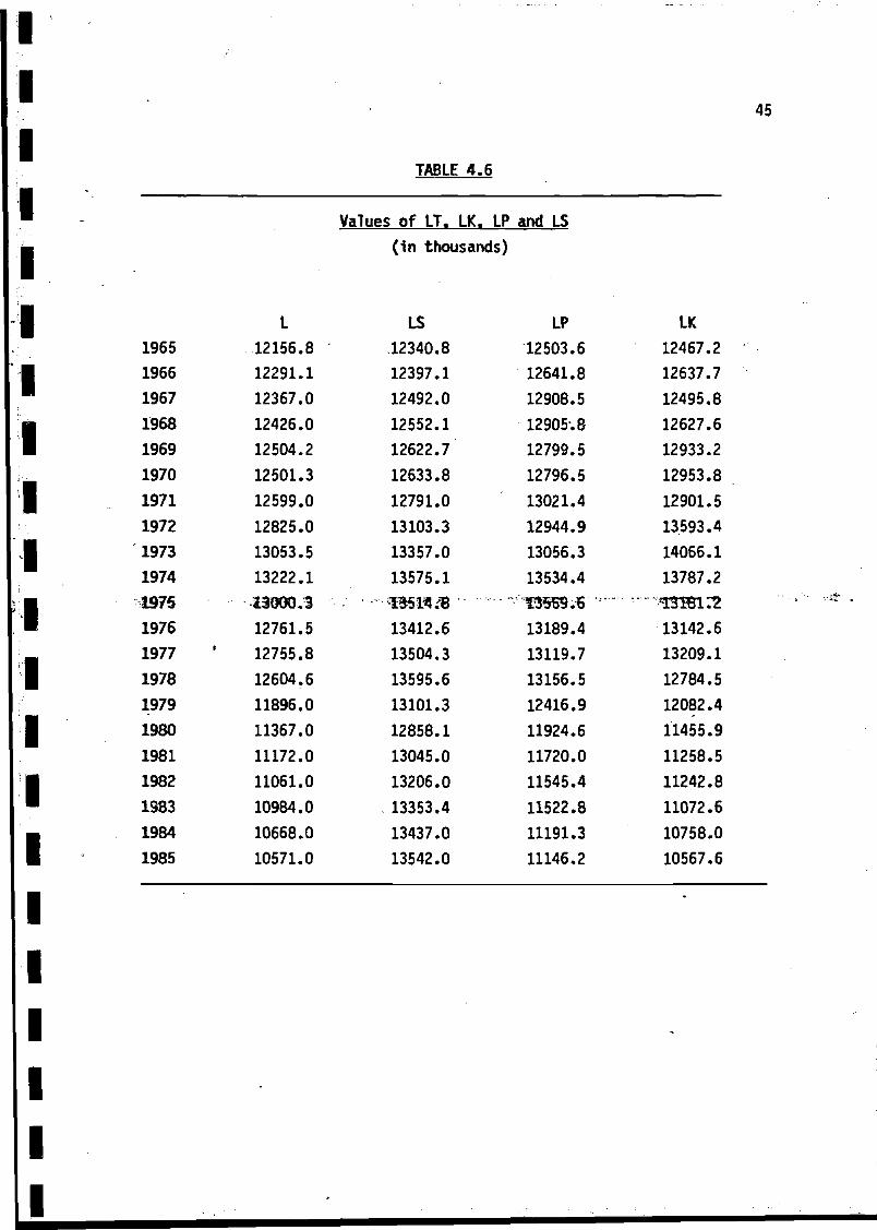
Our estimates of potential employment (LP), Keynesian labourdemand (LK), plus the series of labor force (LS) and employment (L)are shown in Table 4.6 and Figure 2.10 (in Section 2).

•

iIIIIIIIIIIIIIIIIIIII

43

4.2.4. Employment function

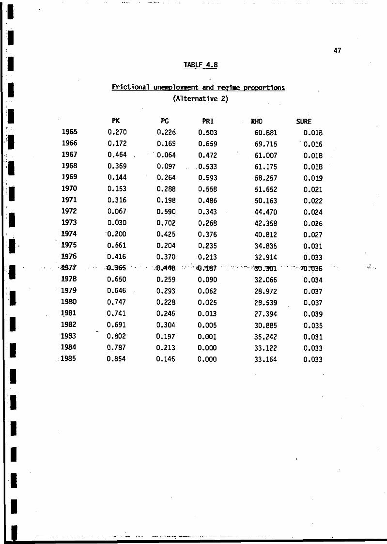
The CES form given 1n (3.11) 1s estimated using 2 alternatives,that we present in Tables 4.5, 4.7 and 4.8. The regime proportionsare shown in Figure 2.12 (in Section 2). The first alternativespecifies the parameter c just as a time trend, while the secondtries to explain this parameters by wage pressure factors. In thesecond alternative we have found an encouraging effect coming fromthe mismatch index MM and changes in the proportion of agriculturalemployment NAN. Under either alternative the results on frictionalunemployment and the shares of firms under Keynesian, Classical orRepressed Inflation are almost identical.

Finally, the implied rate of frictional unemployment is lowerthan expected but similar to the ones obtained in other countriesusing the same model. Both the regime proportions and the frictionalunemployment rate seem to be very robust to alternativespecifications.

TABLE 4.5

IIII

Labour-output relationship

lt = 4.7 + .65 1t-i + -61yt - .40kt -.23at

I (2.5) (3.0) (1,9) (3.2) (1.1)

1 R2 = .97 DW = 1.72 Box-Pierce:X2(10) « 10.1

| Number of observations : 21Degrees of freedom : 16

I Estimation method : Instrumental variables

• Employment equation

_ -Alternative JL:

. e = 33.2 - 6.4t + .19t2

| (8.4) (4.1) (3.1)

I

If - -79.2 + 2.28t - .96MM + 4.07 NAN*

I (2.1) (1.99) (1.19) (3.6) .

I

B agriculture.

I

I

I

I

44

R2 = .997 DM = 1.37

Alternative 2:

R2 - .997 DW = 1.93

*MM is a mismatch Index, NAN the proportion of labour force in

11111"

i1MI111

11•

•11111

TABLE 4

Values of LT. LK

.6

. LP and LS

4!

(in thousands)

196519661967

196819691970

197119721973197419751976197719781979198019811982

198319841985

L12156.812291.112367.012426.012504.212501.312599.012825.013053.513222.113000.312761.512755.812604.611896.011367.011172.011061.010984.010668.010571.0

LS12340.812397.112492.0

12552.112622.7

12633.812791.0

13103.313357.013575.1135W/813412.613504.313595.6

13101.312858.113045.013206.0

. 13353.4

13437.013542.0

LP12503.612641.812908.5

12905-.812799.512796.513021.412944.913056.313534.4

~'!35B9.$ ' " "13189.413119.713156.512416.911924.611720.011545.4

11522.811191.311146.2

LK12467.2 '12637.712495.812627.612933.212953.812901.513593.414066.113787.2

" "í!3TBi:213142.613209.112784.512082.411455.911258.511242.811072.610758.010567.6

*

-

I

1

1

1\ 46

TABLE 4.7

1 Fr1ct1onal unemployment and reqime proportions(Alternative 1)

1•

|

:

11•i

1

1

I

1

1

1

1

1

1

1

1

1

/

1965196619671968196919701971197219731974

19751976mu19781979198019811982

19831984

1985

PK0.2510.169

. 0.4680.3700.1500.1540.317

0.0680.0330.2070.5670.418

• • - • ÍL366

0.6390.6530.7460.7570.6830.7680.7750.851

PC0.2000.1660.0550.0990.2680.2880.2040.5880.6940.4190.2010.3714540.2640.2890.2290.2330.3110.2300.2250.148

PRI0.5490.6650.4770.5320.5820.5580.4780.4440.2730.374

0.2320.211fl.lBO '0.0960.0580.0250.0100.0060.0030.001

0.000

„

RHO76.99471.13465.65960.56855.86051.537

47.59844.04340.87238.08635.68333.664'32.JQ3030.77929.91329.43129.33329.61930.28931.34332.782

SURE0.0140.0150.017 •0.018 -0.0190.0210.0230.0250.0270.0280.0300.032

• ' jTJSZl "'' r '

0.0350.0360.0370.0370.0360.0360.034

0.033

•

I111•

1• - .

1i•ii1

"

ii1'

11•

1111111

TABLE 4.8

47

Frictional uneBDloyieent and reqlwe orooortlons

(Alternative 2)

1965196619671968196919701971197219731974197519764977

19781979198019811982198319841985

: : : :

PK

0.2700.172

0.464 .

0.3690.144

0.153

0.3160.067

0.0300.2000.561

0.41630,365

0.650

0.6460.7470.741

0.691

0.8020.7870.854

- - — - — ..-.-

PC0.226

0.169

0.0640.0970.264

0.2880.198

0.5900.7020.4250.204

0.370

••••••S.'We0.259

0.2930.2280.246

0.3040.197

0.2130.146

— .. _,

PRI

0.503

0.6590.472

0.5330.593

0.5580.486

0.343

0.2680.376

0.235

0.21333ví870.090

0.062

0.0250.013

0.005

0.001

0.0000.000

RHO60.88169.715

61.007

61.17558.257

51.65250.16344.470

42.35840.812

34.83532.914

' "- 80.33132.06628.972

29.53927.394

30.88535.24233.12233.164

SURE

0.018

0.016

0.018

0.0180.019

0.021

0.0220.024

0.0260.027

0.031

0.033

•••-•-•"OITOS ^0.0340.037

0.037

0.039

0.0350.031

0.0330.033

•

1•

1111

. =1••I:

1i. m••

1ii•111111

48.

5. Conclusions

This paper has attempted to provide an explanation of the recent riseof unemployment in Spain. We have approached the problem from severalperspectives, but in all cases basing the explanation on theestimation of a macroeconomic model centered around the labour-.-^andproduction sectors. The main conclusions obtained could be summarizedas follows.

a) Our results suggest that the problem of unemployment in Spain isboth a problem of deficient demand and a problem of deficientcapital stock. In 1985, the main constraint to employment growthwas deficient demand which in that year required a level ofemployment 21.9 per cent below that of labour supply. However,according to our results, demand expansion alone could not have-'solved this • problem, --frs the -extra employment -required -would -very v ;;;

soon have hit the capital constraint. In 1985, without increasingthe capital stock, the maximum amount of employment would stillhave been 17.7 per cent below labour supply.

b) To establish these results we have estimated a model in which theobserved capital -labour ratio depends significantly on relativeprices, on technical progress and on the degree of capacityutilization. Also we have identified correctly signed andsignificant spillover effects coming from the Import and exportequations, which have ennabled us to estimate the "Keynesian"demand for domestic output.

c) We have been less fortunate in the explanation of wages andprices, as the influence of trend productivity on the desiredreal wage is larger than its influence on the feasible real wage,and this implies the existence of a structural element of

iIIIiIiIIIIIIIIIIIIII

49.

inflationary pressure that can only be neutralized by having moreunemployment. Leaving aside this anomalous result, we find thatthe increase of Social Security attributions and real importprices account for more than 45 per cent of the total increase inunemployment experienced between the periods 1972-78 and 1979-85.Cyclical demand also had an important effect on this rise ofunemployment via the real wage (it explains about 12 per cent ofthe total change), but we think that its effect is larger as itmay also operate directly through output demand.

d) The next step should be to explain what determines the level ofaggregate demand and the capital stock, and this in turn impliesto investigate what determines consumption and investment. Weleave that for another paper.

50

ANNEX 1

We present in this Annex the employment equation referred toin Section 2. It has been estimated jointly with the wage and priceequation shown in Section 4.

1 - .52 1_! + .74 k - .51 (w+tl-p)-! - .56 (w+tl-p) + .29 DUK

(3.1) (3.1) (3.9) (3.2) (1.7)

+ .25 A - .025 Trend

(2.2) (2.5)

R2 - .974 ; SEE = .014 ; DW = 2.03 ;

IIIIIIIIIII

51

APPENDIX

LIST OF VARIABLES AND DATA SOURCES

Variables;

A: Labour augmenting technical progress (own estimates).

DUK: Capacity utilization in industry (Survey of Entrepreneur'sOpinions, BE).

D: A truncated trend taking 0 value for 1964-77, T-14.for1978-85.

I: Real imports (in thousands of 1970 pts.) Exports includingtourism expenditures (INE.CN).

10 : Real oil Imports (in Thousand 1970 pts.). Oil imports (BE)divided by the oil imports unit value (MECO).

INO: Real non-oil imports (in thousands 1970 pts.). Non-oilImports (BE) divided by the implicit non-oil imports de-flator obtained from the imports deflator and the oilimports deflator.

1CLS: ' Capitalflaboar -supply Tatio.'"Capital -series -fawn stTmates)divided by labour supply (thousands)(INE,EPA).

1mm

1

L : Number of employed (in thousan

ÍW : An index of mismatch. Sumproportion of total employeestotal employees (GTE and EPA).

ds) (EPA).

of absolute changes in thein each sector relative to

KAN : Proportion of agricultural labor force (GTE and EPA).

1•P

11•

1

1

1

1

PIP: ••••• Relative price of investment; '"flator divided by GDP deflator

•Gross fixed investment de-•

PREL: Ratio of CPI (INE) to GDP deflator (market prices) minusindirect taxes (INE.CN).

PRME: Relative price of oil imports.by GDP deflator.

Oil imports deflator divided

PRMC: Relative price of consumption imports goods. Consumptionimportables unit value divided by GDP deflator.

•

IIIIII

I1IIIIIIIIIII

52

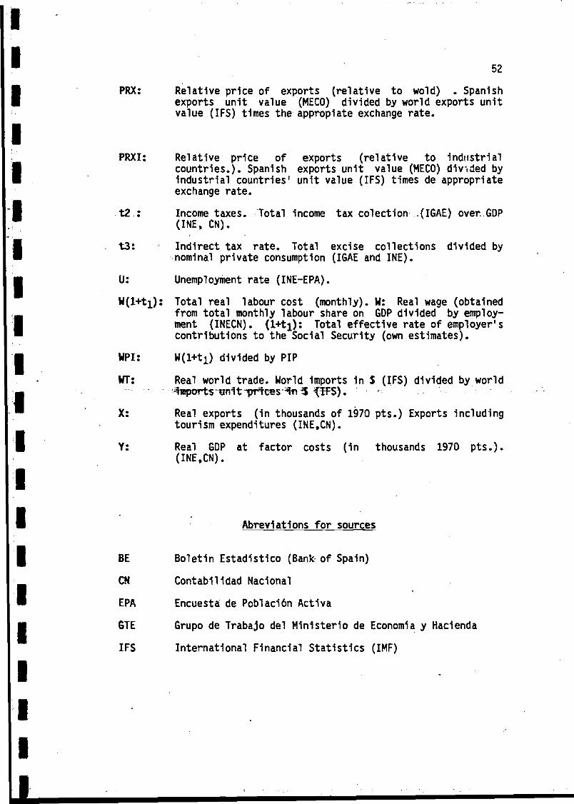
PRX: Relative price of exports (relative to wold) . Spanishexports unit value (MECO) divided by world exports unitvalue (IPS) times the appropriate exchange rate.

PRXI: Relative price of exports (relative to industrialcountries.). Spanish exports unit value (MECO) divided byindustrial countries' unit value (IPS) times de appropriateexchange rate.

t2 : Income taxes. Total income tax colection .(IGAE) over..-GDP(INE, CN).

t3: Indirect tax rate. Total excise collections divided bynominal private consumption (IGAE and INE).

U: Unemployment rate (INE-EPA).

H(l+ti): Total real labour cost (monthly). H: Real wage (obtainedfrom total monthly labour share on GDP divided by employ-ment (INECN). (1+ti): Total effective rate of employer'scontributions to the Social Security (own estimates).

HPI: W(H-ti) divided by PIP

HT: Real world trade. World imports in $ (IPS) divided by world•%!ports n1tT3rtces %!$ fIFS).

X: Real exports (in thousands of 1970 pts.) Exports includingtourism expenditures (INE.CN).

Y: Real GDP at factor costs (1n thousands 1970 pts.).(INE.CN).

Abreviations for sources

BE Boletin Estadistico (Bank of Spain)

CN Contabilidad Nacional

EPA Encuesta de Población Activa

GTE Grupo de Trabajo del Ministerio de Economía y Hacienda

IPS International Financial Statistics (IMF)

II• MECO Ministerio de Comercio

IGAE Intervención General de la Administración del Estado

jj INE Instituto Nacional de Industria

iII¡

IiI1' • ' *

iIIIiIIII

54

REFERENCES

BEAN, C. and 6AVOSTO, A.(1987): "A discussion of British Unemploymentcombining traditional concepts and disequilibrium economics: apreliminary .report", CLE Working Paper.No.976.

BONILLA, J.M. (1978): "Funciones de Importación y Exportación para'laeconomía española", Estudios Económicos. No. 14,, Banco de fspaña.

DOLADO, J.J.; MALO DE MOLINA, J.L. and ZABALZA, A.(1986): "SpanishIndustrial Unemployment: Some Explanatory Factors", Económica Vol.53,No. 210.

LAMBERT, P. (1987): "Disequilibrium Macro Models", CambridgeUniversity Press. Cambridge.

MAULEON, I. (1985): "Análisis econométrico de las importacionesespañolas". Documento Interno Servicio de Estudios. Banco de España.

MAULEON, I. (1986): "Una función de exportación para la economíaespañola", Investigaciones Económicas, vol. X, No. 2, pág. 357-378.

MOLINAS, C.; SEBASTIAN, M. and ZABALZA, A. (1987): "European•Unemployment Program: preliminary results- on Spanish Unemployment",manuscript.

SNEESSENS, H.R. and DREZE, J.H. (1986): "A Discussion of BelgianUnemployment Combining Traditional Concepts and DisequilibriumEconomics", Económica. Vol. 53, No. 210.

SNEESSENS, H.R. and DREZE, J.H. (1987): "Report on the Project onEuropean Unemployment", CORE, manuscript.