io.1

EEL-4713Computer Architecture

I/O Systems

io.2

Outline

° I/O Performance Measures

° Types and Characteristics of I/O Devices

° Magnetic Disks

° Summary

io.3

The Big Picture: Where are We Now?

Control

Datapath

Memory

Processor

Input

Output

° Today’s Topic: I/O Systems

Control

Datapath

Memory

Processor

Input

Output

Network

io.4

I/O System Design Issues

Processor

Cache

Memory - I/O Bus

MainMemory

I/OController

Disk Disk

I/OController

I/OController

Graphics Network

interrupts

• Performance

• Expandability

• Resilience in the face of failure

io.5

Types and Characteristics of I/O Devices

° Behavior: how does an I/O device behave?

• Input: read only

• Output: write only, cannot read

• Storage: can be reread and usually rewritten

° Partner:

• Either a human or a machine is at the other end of the I/O device

• Either feeding data on input or reading data on output

° Data rate:

• The peak rate at which data can be transferred:

- Between the I/O device and the main memory

- Or between the I/O device and the CPU

io.6

I/O Device Examples

Device Behavior Partner Data Rate (MBit/sec)

Keyboard Input Human 0.0001

Mouse Input Human 0.004

Graphics Display Output Human 800-8000

Network-LAN Input or Output Machine 100-1000

Wireless LAN Input or Output Machine 11-54

Optical Disk Storage Machine 80

Magnetic Disk Storage Machine 340-2560

io.7

Magnetic Disk

° Purpose:

• Long term, nonvolatile storage

• Large, inexpensive, and slow

• Lowest level in the memory hierarchy

° Hard disks:

• Rely on a rotating platter coated with a magnetic surface

• Use a moveable read/write head to access the disk

• Platters are rigid ( metal or glass)

• High density

• High data access rate: disks spin fast, plus can incorporate more than one platter and r/w head

Registers

Cach

e

Mem

ory

Disk

io.8

Organization of a Hard Magnetic Disk

° Typically, 10,000-50,000 tracks per surface

• 100-500 sectors per track

° A sector is the smallest unit that can be read/written

• 512Bytes – 4096Bytes

° Early days: all tracks had the same number of sectors

• Zone bit recording: record more sectors on the outer tracks

Platters

Track

Sector

io.9

Magnetic Disk Characteristic

° Cylinder: all the tracks under the head at a given point on all surface

° Read/write data is a three-stage process:

• Seek time: position the arm over the proper track

• Rotational latency: wait for the desired sectorto rotate under the read/write head

• Transfer time: transfer a block of bits (sector)under the read-write head

° Average seek time as reported by the industry:

• Typically in the range of 3 ms to 14 ms

• (Sum of the time for all possible seek) / (total # of possible seeks)

° Due to locality of disk reference, actual average seek time may:

• Only be 25% to 33% of the advertised number

SectorTrack

Cylinder

HeadPlatter

io.10

Typical Numbers of a Magnetic Disk

° Rotational Latency:

• Most disks rotate at 5K-15K RPM

• Approximately 4-12ms per revolution

• An average latency to the desiredinformation is halfway around the disk

° Transfer Time is a function of :

• Transfer size (usually a sector): 512B-4KB / sector

• Rotation speed (5K-15K RPM)

• Recording density: typical diameter ranges from 2 to 3.5 in

• Typical values: 30-80 MB per second

- Caches near disk; higher bandwidth (320MB/s)

SectorTrack

Cylinder

HeadPlatter

io.1104/18/23 11

Future Disk Size and Performance

° Capacity growth (60%/yr) overshoots bandwidth growth (40%/yr)

° Slow improvement in seek, rotation (8%/yr)

° Time to read whole disk

Year Sequentially Randomly (latency) (bandwidth) (1 sector/seek)

1990 4 minutes 6 hours

2000 12 minutes 1 week(!)

2006 56 minutes 3 weeks (SCSI)

2006 171 minutes 7 weeks (SATA)

° Disks are now like tapes, random access is slow!

3x

4.6x

3x

24x

3x

2.3x

io.12

Disk I/O Performance

° Disk Access Time = Seek time + Rotational Latency + Transfer time

+ Controller Time + Queueing Delay

° Estimating Queue Length:

• Will see later

ProcessorQueue

DiskController

Disk

Service RateRequest Rate

Queue

DiskController

Disk

io.14

I/O System Performance

° I/O System performance depends on many aspects of the system:

• The CPU

• The memory system:

- Internal and external caches

- Main Memory

• The underlying interconnection (buses)

• The I/O controller

• The I/O device

• The speed of the I/O software

• The efficiency of the software’s use of the I/O devices

° Two common performance metrics:

• Throughput: I/O bandwidth

• Response time: Latency

io.15

Bandwidth/latency example

° Which has higher bandwidth?

• You are driving to Tallahassee to visit a friend. You carry two DVD-ROMs

• A 1Mbit/s cable modem link to your ISP and high-bandwidth, fiber-optic backbone connecting ISP to FSU

io.16

Car + DVD bandwidth

° Data:

• One DVD: 3250MBytes

• Two DVDs: 2*3250M*8 = 52Gbits

° Time:

• 140 miles

• 70 mph

• 2 hours

° Bandwidth:

• (52*10^9) / (2*60*60) = 7.2 Mbit/s

io.17

Car vs. cable° Car has higher bandwidth!

° Latency?

• How long before your friend will see first chapter of first DVD?

• Hours vs. seconds

• Cable modem has smaller latency

io.18

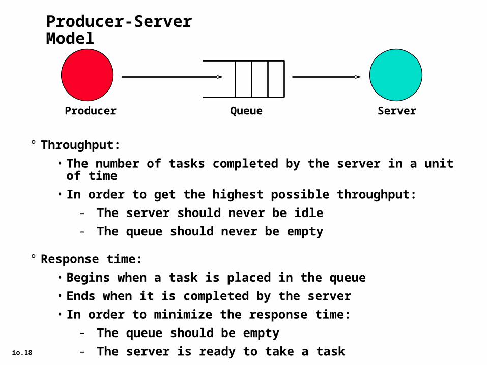
Producer-Server Model

° Throughput:

• The number of tasks completed by the server in a unit of time

• In order to get the highest possible throughput:

- The server should never be idle

- The queue should never be empty

° Response time:

• Begins when a task is placed in the queue

• Ends when it is completed by the server

• In order to minimize the response time:

- The queue should be empty

- The server is ready to take a task

Producer ServerQueue

io.19

Latency vs. throughput

Increasedload (requests)

7x factor

io.20

Throughput Enhancement

° In general throughput can be improved by:

• Throwing more hardware at the problem

° Response time is much harder to reduce:

• Ultimately it is limited by the speed of light

Producer

ServerQueue

QueueServer

io.21

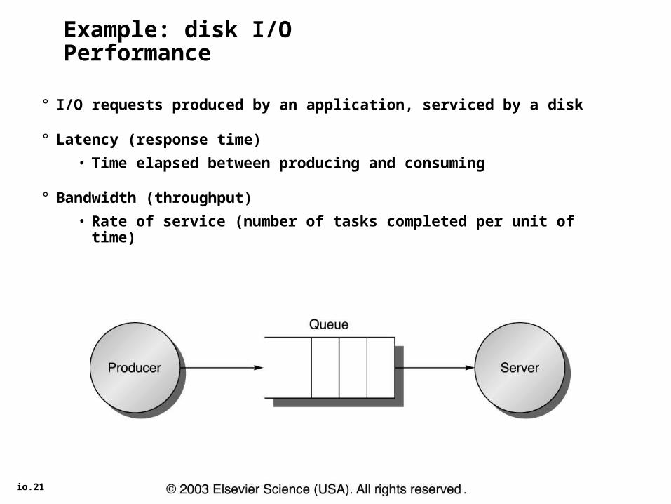
Example: disk I/O Performance

° I/O requests produced by an application, serviced by a disk

° Latency (response time)

• Time elapsed between producing and consuming

° Bandwidth (throughput)

• Rate of service (number of tasks completed per unit of time)

io.22

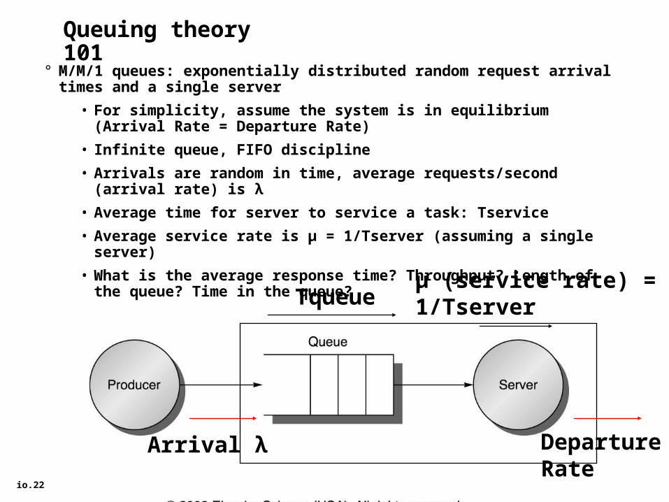
Queuing theory 101

° M/M/1 queues: exponentially distributed random request arrival times and a single server

• For simplicity, assume the system is in equilibrium (Arrival Rate = Departure Rate)

• Infinite queue, FIFO discipline

• Arrivals are random in time, average requests/second (arrival rate) is λ

• Average time for server to service a task: Tservice

• Average service rate is µ = 1/Tserver (assuming a single server)

• What is the average response time? Throughput? Length of the queue? Time in the queue?

Arrival λ DepartureRate

µ (service rate) = 1/TserverTqueue

io.23

Latency

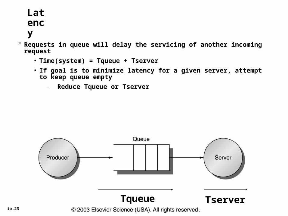
° Requests in queue will delay the servicing of another incoming request

• Time(system) = Tqueue + Tserver

• If goal is to minimize latency for a given server, attempt to keep queue empty

- Reduce Tqueue or Tserver

Tqueue Tserver

io.24

Throughput° An empty queue will make the server idle

• If goal is to maximize throughput, must maximize the utilization of the server

- Always have requests on the queue

Tqueue Tserver

io.25

Queuing theory 101

° Length or number of tasks in each area

• LengthServer = average number of tasks in service

• LengthQueue = Average length of the queue = λ*Tqueue

• LengthSystem = LengthServer + LengthQueue

Arrival λ departure

Tqueue µ (service rate) = 1/Tserver

io.26

Queuing theory 101

° How busy is the server?

• Server utilization must be between 0 and 1 for a system in equilibrium; AKA traffic intensity ρ

• Server utilization ρ = mean number of tasks in service = λ (arrival rate) * Tserver

• Example: What is disk utilization if get 50 I/O requests per second for disk and average disk service time is 10 ms (0.01 sec)?

- Server utilization = 50/sec x 0.01 sec = 0.5

- Or server is busy on average 50% of time

Arrival λ departure

Tqueue µ (service rate) = 1/Tserver

io.27

Time in Queue vs. Queue Latency

° FIFO queue

° Tqueue = LengthQueue * Tserver + “Mean time to complete service of task when a new task arrives if the server is busy (residual service time)”

° New task can arrive at any instance; how do we predict the residual service time

° To predict performance, need to know something about distribution of events….but that is outside the scope of this class so we move straight to …

Arrival λ departure

Tqueue µ (service rate) = 1/Tserver

io.28

Time in Queue

Arrival λ departure

Tqueue µ (service rate) = 1/Tserver

° All tasks in queue (QueueLength) ahead of new task must be completed before task can be serviced

• Each task takes on average Tserver

• Task at server takes average residual service time to complete

° Chance server is busy is server utilization expected time for service is Server utilization Average residual service time

° Tqueue = QueueLength x Tserver + Server utilization x Average residual service time

° Substituting definitions for QueueLength, Average residual service time, & rearranging:

Tqueue = Tserve x Server utilization/(1-Server utilization)

° So, given a set of I/O requests, you can determine how many disks you need

io.2904/18/23 29

M/M/1 Queuing Model

° System is in equilibrium

° Times between 2 successive requests arriving, “interarrival times”, are exponentially distributed

° Number of sources of requests is unlimited “infinite population model”

° Server can start next job immediately

° Single queue, no limit to length of queue, and FIFO discipline, so all tasks in line must be completed

° There is one server

° Called M/M/1

1. Exponentially random request arrival

2. Exponentially random service time

3. 1 server

• M standing for Markov, mathematician who defined and analyzed the memoryless processes

io.3004/18/23 30

Example 1

° 40 disk I/Os / sec, requests are exponentially distributed, and average service time is 20 ms

Arrival rate/sec = 40, Timeserver = 0.02 sec

1. On average, how utilized is the disk?

° Server utilization = Arrival rate Tserver = 40 x 0.02 = 0.8 = 80%

2. What is the average time spent in the queue?

° Tqueue = Tserverx Server utilization/(1-Server utilization)

= 20 ms x 0.8/(1-0.8) = 20 x 4 = 80 ms

° What is the average response time for a disk request, including the queuing time and disk service time?

° Tsystem = Tqueue + Tserver = 80+20 ms = 100 ms

io.3104/18/23 31

Example 2: How much better with 2X faster disk?

° Average service time is 10 ms

Arrival rate/sec = 40, Timeserver = 0.01 sec

1. On average, how utilized is the disk?

° Server utilization = Arrival rate Timeserver = 40 x 0.01 = 0.4 = 40%

° What is the average time spent in the queue?

° Tqueue= Tserverx Server utilization/(1-Server utilization)

= 10 ms x 0.4/(1-0.4) = 10 x 2/3 = 6.7 ms

° What is the average response time for a disk request, including the queuing time and disk service time?

° Tsystem=Tqueue+ Tserver =6.7+10 ms = 16.7 ms

° 6X faster response time with 2X faster disk!

io.3204/18/23 32

Value of Queueing Theory in practice

° Learn quickly do not try to utilize resource 100% but how far should back off?

° Allows designers to decide impact of faster hardware on utilization and hence on response time

° Works surprisingly well

io.33

I/O Benchmarks for Magnetic Disks

° Supercomputer application:

• Large-scale scientific problems

° Transaction processing:

• Examples: Airline reservations systems and banks

° File system:

• Example: UNIX file system

io.34

Supercomputer I/O

° Supercomputer I/O is dominated by access to large files on magnetic disks

° The overriding supercomputer I/O measures is data throughput:

• Bytes/second that can be transferred between disk and memory

io.35

Transaction Processing I/O

° Transaction processing:

• Examples: airline reservations systems, bank ATMs

• A lot of small changes to a large body of shared data

° Transaction processing requirements:

• Throughput and response time are both important

° Transaction processing is chiefly concerned with I/O rate:

• The number of disk accesses per second

° Each transaction in typical transaction processing system takes:

• Between 2 and 10 disk I/Os

• Between 5,000 and 20,000 CPU instructions per disk I/O

io.36

File System I/O

° Measurements of UNIX file systems in an engineering environment:

• 80% of accesses are to files less than 10 KB

• 90% of all file accesses are to data with sequential addresses on the disk

• 67% of the accesses are reads

• 27% of the accesses are writes

• 6% of the accesses are read-write accesses

io.37

*Reliability and Availability

° Two terms that are often confused:

• Reliability: Is anything broken?

• Availability: Is the system still available to the user?

° Availability can be improved by adding hardware:

• Example: adding ECC to memory

° Reliability can only be improved by:

• Bettering environmental conditions

• Building more reliable components

• Building with fewer components

- Improved availability may come at the cost of lower reliability

io.38

Disk Arrays

° An array organization of disk storage (RAID):

• Arrays of small and inexpensive disks

• Increase potential throughput by having many disk drives:

- Data is spread over multiple disks

- Multiple accesses are made to several disks

° Reliability is lower than a single disk:

• But availability can be improved by adding redundant disks:Lost information can be reconstructed from redundant information

io.39

What is a failure?

° The user perception of a service does not match its specified behavior

° Decomposition: faults, errors and failure

• Failures are caused by errors

• Errors are caused by faults

• But, the inverse is not necessarily true:

- Faults cause “latent” errors that may never be activated

- Errors may not cause failures

io.40

Example

° A DRAM transistor loses its charge between refresh cycles

• A fault

° Its consequence is a latent error

• It is not activated if no program loads this memory word

° If this memory word is loaded:

• The load returns an erroneous word

• Not a failure until manifested in the service

- E.g. what if the faulty bit is masked with an AND operation in an application?

io.41

Reliability, availability and RAID

° Storage devices are slower than CPU, memory

• Parallelism can also be exploited in this case for improving throughput/bandwidth

- Not the speed of a single request

° Motivations for disk arrays:

• High storage capacity

• Potential overlapping of multiple disk operations (seek, rotate, transfer) for high throughput

• Best price/gigabyte on small/medium disks that are sold in high volume

io.42

Reliability issues

° But, computer systems are prone to failure

• Hardware, software, operator

- In particular, disks, moving parts

• More components (array) - increased probability of system failure

io.43

Reliability/Availability

° Reliability: measure of continuous service until a failure

• Mean time to failure (MTTF) is an average measurement of a typical component’s reliability

° Availability: measure of continuous service with respect to the continuous and interrupted intervals

• MTTF/(MTTF+MTTR)

- MTTR: mean time to repair

io.44

System reliability

° If individual modules have exponentially distributed lifetimes:

• FIT (Failures in Time or Failure rate ) = 1/MTTF

° A system’s failure distribution:

• If independent, exponential distribution

- System total = Product of reliability distributions of individual components

- Resulting failure rate is the sum of each module’s failure rate

° Example: 10 disks, each MTTF=5 years

• FIT (disk) = 1/5 (1/year)

• FIT (system) = 1/5 (1/year) * 10 disks = 2 (disks/year)

• MTTF (system) = 1/2 year/disk

io.45

Example° A disk has MTTF of 100 days, MTTR of 1 day

• Availability = 100/101 = 99%

° If you have two disks storing different parts of your data

• MTTF(1 disk) still 100 days

• MTTF(2 disks) = 100/2 = 50 days

• Availability = 50/51 = 98%

° What if the second disk “mirrors” the first and each one can take over on failure of the other?

• MTTF(1 disk) still 100 days

• Assuming failed disks are repaired at same MTTR, availability is a function of the probability that both disks fail within the same day

- Each disk’s availability is 99%, so only a 1% chance of failure for 1 and a 1%*1% = .01% chance of failure of both

- MTTF both disks = 100 days * 100 days = 10,000 days

- 10000/(10000+1) = 99.99%

io.4604/18/23 46

Quantifying Availability

Availability

90.%

99.%

99.9%

99.99%

99.999%

99.9999%

99.99999%

System Type

Unmanaged

Managed

Well Managed

Fault Tolerant

High-Availability

Very-High-Availability

Ultra-Availability

Unavailable(min/year)

50,000

5,000

500

50

5

.5

.05

AvailabilityClass

1234567

UnAvailability = MTTR/MTBFcan cut it in ½ by cutting MTTR or MTBF

From Jim Gray’s “Talk at UC Berkeley on Fault Tolerance " 11/9/00

io.4704/18/23 47

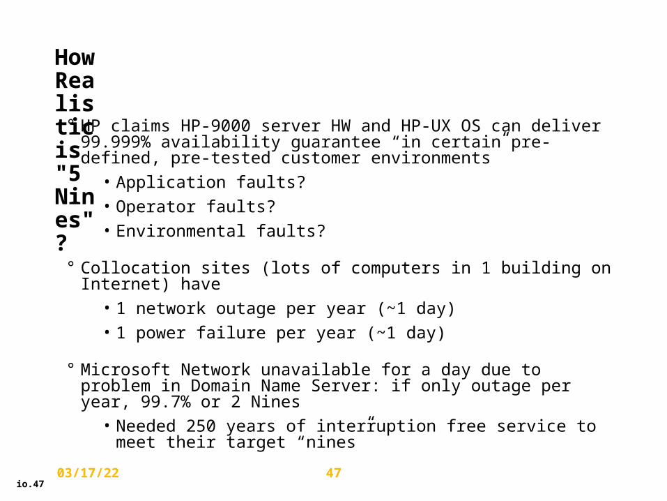
How Realistic is "5 Nines"?

° HP claims HP-9000 server HW and HP-UX OS can deliver 99.999% availability guarantee “in certain pre-defined, pre-tested customer environments”

• Application faults?

• Operator faults?

• Environmental faults?

° Collocation sites (lots of computers in 1 building on Internet) have

• 1 network outage per year (~1 day)

• 1 power failure per year (~1 day)

° Microsoft Network unavailable for a day due to problem in Domain Name Server: if only outage per year, 99.7% or 2 Nines

• Needed 250 years of interruption free service to meet their target “nines”

io.48

MTTF Implications

° Disk arrays have shorter MTTFs

• But are desirable for performance/capacity reasons

° Approach: use redundancy to improve availability in disk arrays

• Redundant Array of Inexpensive Disks (RAID)

io.4904/18/23 49

The case for RAID in the past:Manufacturing Advantages of Disk Arrays (1987)

° Conventional: 4 disk designs (4 product teams):

° Disk array: 1 disk design

Low end -> high end (main frame)

3.5” 5.25”10”

14”

3.5”

But is there a catch??

io.5004/18/23 50

The case for RAID in the past:Arrays of Disks to Close the Performance Gap (1988 disks)

° Replace small number of large disks with a large number of small disks

° Data arrays have potential for

• Large data and I/O rates

• High MB per cu. ft

• High MB per KW

IBM 3380 Smaller disk Smaller disk x50

Data Capacity 7.5 GBytes 320 MBytes 16 GBytes

Volume 24 cu. ft. 0.2 cu. ft. 20 cu. ft

Power 1.65 KW 10 W 0.5 KW

Data Rate 12 MB/s 2 MB/s 100 MB/s

I/O Rate 200 I/Os/s 40 I/Os/s 2000 I/Os/s

Cost $100k $2k $100k

io.5104/18/23 51

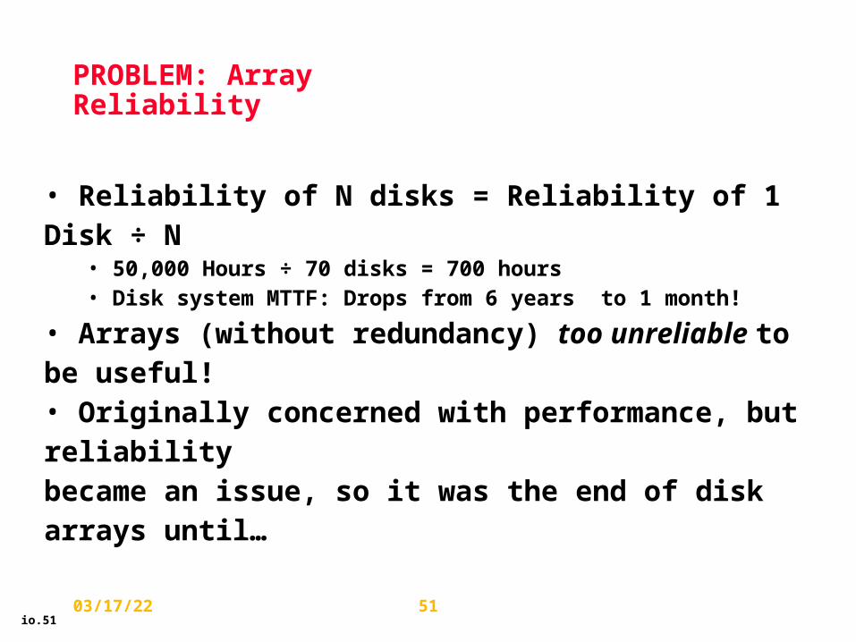
PROBLEM: Array Reliability

• Reliability of N disks = Reliability of 1 Disk ÷ N• 50,000 Hours ÷ 70 disks = 700 hours• Disk system MTTF: Drops from 6 years to 1 month!

• Arrays (without redundancy) too unreliable to be useful!• Originally concerned with performance, but reliability became an issue, so it was the end of disk arrays until…

io.5204/18/23 52

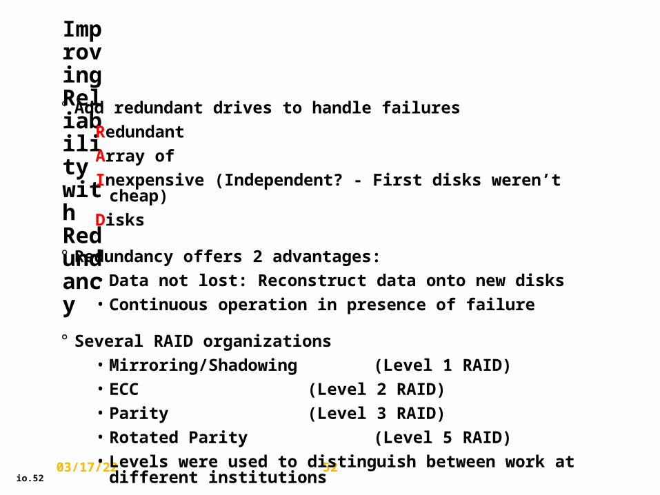
Improving Reliability with Redundancy

° Add redundant drives to handle failures

Redundant

Array of

Inexpensive (Independent? - First disks weren’t cheap)

Disks

° Redundancy offers 2 advantages:

• Data not lost: Reconstruct data onto new disks

• Continuous operation in presence of failure

° Several RAID organizations

• Mirroring/Shadowing (Level 1 RAID)

• ECC (Level 2 RAID)

• Parity (Level 3 RAID)

• Rotated Parity (Level 5 RAID)

• Levels were used to distinguish between work at different institutions

io.53

Key: Reliability with redundancy

° Do not use all space available to store data

• Also store information that can be used to prevent faults from becoming failures

° Technique used in other computing/ communications systems

• Error-correction codes

• E.g. the parity bit in a DRAM can be used to detect single-bit faults

io.54

MTTF and MTTR

° Disks have MTTRs that are much shorter than MTTFs

• Hours (MTTR) vs. years (MTTF)

• Redundancy allows system to tolerate one or more faults while a defective device (e.g. a hot-swappable disk) is replaced

io.55

Notes

° Faults are not avoided by redundancy

• Improvements in fault rates only achieved with better manufacturing/environmental conditions

° Redundancy is used to prevent errors from becoming failures

• Reliability of a system vs. individual components

° Redundancy adds cost:

• Need to purchase more storage capacity

• Need to spend more power

• Design complexity (Has a fault occurred? Who takes over? How to restore state once repaired?)

° But, redundancy can help improve performance

• Mirrored disks – easy to split read requests

io.56

RAID redundancy

° Several “levels” of RAID can be implemented and configured in a given controller

• Tradeoffs in controller complexity, fault tolerance and performance

° RAID0

• No redundancy – plain disk array

- Best performance, simplest, but a faulty disk activates an error if accessed

io.57

RAID 1

° Mirrored redundancy

• Data written to disk A is always written to mirror disk A’

• Uses 2N X-Byte disks to store N*X Bytes of information

• Bandwidth sacrifice

• 100% overhead!

A

A’

io.58

RAID 3

° Bit-interleaved parity

• Store striped parity across all disks on one parity disk

• Ex: Xor all bits

° Rely on interface to know which disk failed

° Does not store entire copy of data in redundant disk

• Just enough information to recover/recreate data in case of a fault

• One disk holds blocks containing the parity sum of blocks of other disks

- N+1 X-Byte disks to store N*X Bytes

• Can avoid failures from a single fault

P

P

P

io.59

Parity example

Data (disks 1-4)

1: 00000011

2: 00001111

3: 11000011

4: 11111111

Parity (disk 5):

5: 00110000

When reading data,also calculate parity (xor)if 0, OK;if 1, fault

io.60

Parity example

Disk 3 fails

1: 00000011

2: 00001111

3: 11000011

4: 11111111

Parity (disk 5):

5: 00110000

How to recover 3’s datafrom 1, 2, 4, 5?

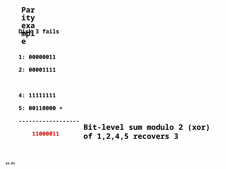
io.61

Parity example

Disk 3 fails

1: 00000011

2: 00001111

4: 11111111

5: 00110000 +

------------------

11000011Bit-level sum modulo 2 (xor)of 1,2,4,5 recovers 3

io.62

Inspiration for RAID 4

° RAID 3 relies on parity disk to discover errors on read – parity disk is a bottleneck

° But every sector (on each disk) has its own error detection field

° To catch errors on read, could just rely on error detection field on the disk

• Allows independent reads to different disks simultaneously, parity disk is no longer a bottleneck on reads

• Still need to update on writes

° Define:• Small read/write - read/write to one disk

- Applications are dominated by these

• Large read/write - read/write to more than one disk

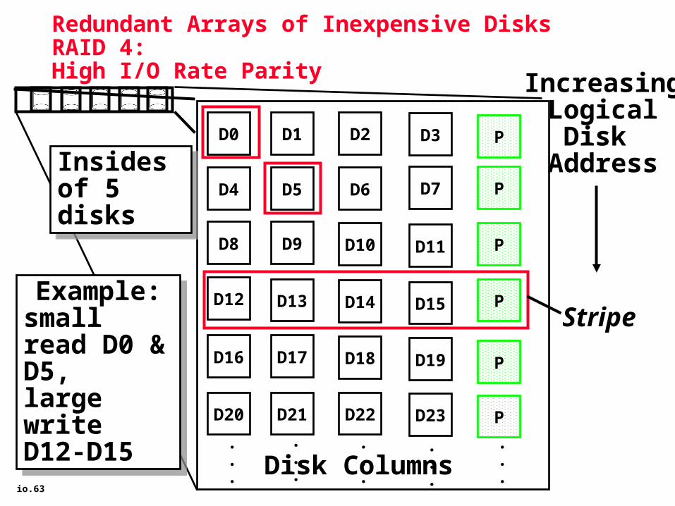
io.63

Redundant Arrays of Inexpensive Disks RAID 4:

High I/O Rate Parity

D0 D1 D2 D3 P

D4 D5 D6 PD7

D8 D9 PD10 D11

D12 PD13 D14 D15

PD16 D17 D18 D19

D20 D21 D22 D23 P

.

.

.

.

.

.

.

.

.

.

.

.

.

.

.Disk Columns

IncreasingLogicalDisk

Address

Stripe

Insides of 5 disksInsides of 5 disks

Example:small read D0 & D5, large write D12-D15

Example:small read D0 & D5, large write D12-D15

io.64

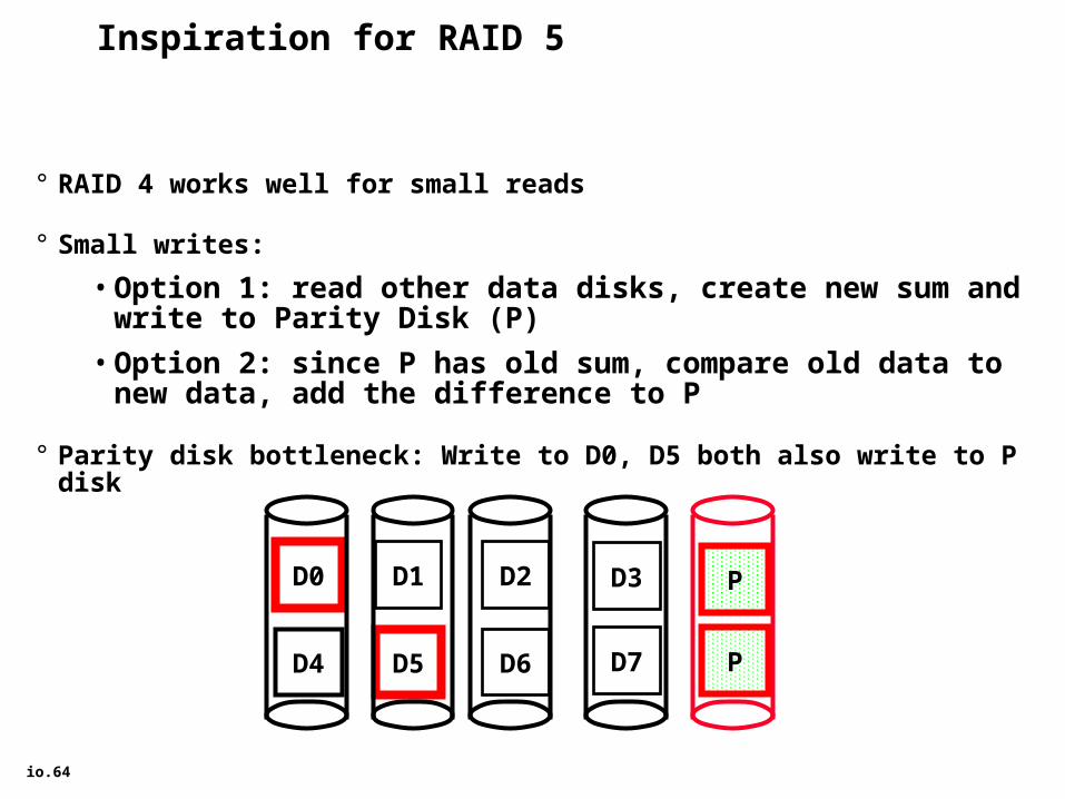
Inspiration for RAID 5

° RAID 4 works well for small reads

° Small writes:

• Option 1: read other data disks, create new sum and write to Parity Disk (P)

• Option 2: since P has old sum, compare old data to new data, add the difference to P

° Parity disk bottleneck: Write to D0, D5 both also write to P disk

D0 D1 D2 D3 P

D4 D5 D6 PD7

io.65

Problems of Disk Arrays: Option 2 for Small Writes

D0 D1 D2 D3 PD0'

+

+

D0' D1 D2 D3 P'

newdata

olddata

old parity

XOR

XOR

(1. Read) (2. Read)

(3. Write) (4. Write)

1 Logical Write = 2 Physical Reads + 2 Physical Writes

io.66

Redundant Arrays of Inexpensive Disks RAID 5:

High I/O Rate Interleaved Parity

Independent writespossible because ofinterleaved parity

Independent writespossible because ofinterleaved parity

D0 D1 D2 D3 P

D4 D5 D6 P D7

D8 D9 P D10 D11

D12 P D13 D14 D15

P D16 D17 D18 D19

D20 D21 D22 D23 P

.

.

.

.

.

.

.

.

.

.

.

.

.

.

.Disk Columns

IncreasingLogical

Disk Addresses

Example: write to D0, D5 uses disks 0, 1, 3, 4

io.67

RAID 6: Recovering from 2 failures

° RAID 6 was always there but not so popular

• Has recently become more popular. Why?

° Recover from more than 1 failure - Why?

• Operator might accidentally replaces the wrong disk during a failure

• since disk bandwidth is growing more slowly than disk capacity, the MTTR a disk in a RAID system is increasing

- Long time to copy data back to disk after replacement

- increases the chances of a 2nd failure during repair since takes longer

• reading much more data during reconstruction meant increasing the chance of an uncorrectable media failure, which would result in data loss

- Uncorrectable error - ECC doesn‘t catch. Insert another error

io.68

RAID 6: Recovering from 2 failures

° Recovering from 2 failures

• Network Appliance’s (make NSF file servers primarily) row-diagonal parity or RAID-DP

° Like the standard RAID schemes, it uses redundant space based on parity calculation per stripe

° Since it is protecting against a double failure, it adds two check blocks per stripe of data.

• 2 check disks - row and diagonal parity

• 2 ways to calculate parity

° Row parity disk is just like in RAID 4

• Even parity across the other n-2 data blocks in its stripe

• So n-2 disks contain data and 2 do not for each parity stripe

° Each block of the diagonal parity disk contains the even parity of the blocks in the same diagonal

• Each diagonal does not cover 1 disk, hence you only need n-1 diagonals to protect n disks

io.69

Example

Data Disk 0

Data Disk 1

Data Disk 2

Data Disk 3

Row Parity

Diagonal Parity

0 1 2 3 4 0

1 2 3 4 0 1

2 3 4 0 1 2

3 4 0 1 2 3

4 0 1 2 3 4

0 1 2 3 4 0

• Assume disks 1 and 3 fail• Can’t recover using row parity because 2 data blocks are missing• However, we can use diagonal parity 0 since it covers every disk

except disk 1, thus we can recover some information on disk 3• Recover in an iterative fashion, alternating between row and diagonal

parity recovery

Fail! Fail!

1. Diagonal 0 misses disk 1, so data can be recovered in disk 3 from row 0.

0

2. Diagonal 2 misses disk 3, so data can be recovered in disk 1 from diagonal 2.

2

3. Standard RAID recovery can now recover rows 1 and 2.

4

3

4. Diagonal parity can now recover row 3 and 4 in disks 3 and 1 respectively

3

4

5. Finally, standard RAID recover can recover rows 0 and 3

1

1