ACTAUNIVERSITATIS

UPSALIENSISUPPSALA

2014

Digital Comprehensive Summaries of Uppsala Dissertationsfrom the Faculty of Science and Technology 1116

Inversion and Joint Inversion ofElectromagnetic and PotentialField Data

JOCHEN KAMM

ISSN 1651-6214ISBN 978-91-554-8856-7urn:nbn:se:uu:diva-215673

Dissertation presented at Uppsala University to be publicly examined in Hambergsalen,Geocentrum, Villavägen 16, Uppsala, Friday, 28 February 2014 at 10:00 for the degree ofDoctor of Philosophy. The examination will be conducted in English. Faculty examiner:Professor Douglas Oldenburg (University of British Columbia).

AbstractKamm, J. 2014. Inversion and Joint Inversion of Electromagnetic and Potential Field Data.(Inversion und kombinierte Inversion von elektromagnetischen und Potentialfelddaten).Digital Comprehensive Summaries of Uppsala Dissertations from the Faculty of Science andTechnology 1116. 108 pp. Uppsala: Acta Universitatis Upsaliensis. ISBN 978-91-554-8856-7.

In this thesis, four inversion problems of different scale and difficulty are solved. Two of themare electromagnetic inverse problems. Two more are joint inversion problems of potential fielddata and other types of data. First, a linear approximation, which is a generalization of the low-induction-number approximation standard in slingram dual-loop interpretation is developed andused for rapid two and three dimensional inversion. The approximation takes induction withina background half-space into account and can thus be applied in conductive scenarios, whereotherwise a rigorous electromagnetic modeling would be required. Second, a three-dimensionalinversion of airborne tensor very-low-frequency data with a rigorous forward modeling at itscore is developed. For dealing with the large scale of the forward problem, a nested fast-Fourier-transform-based integral equation method is introduced, wherein electromagnetic interactionsare arranged according to their range and larger ranges are treated with less accuracy and effort.The inversion improves the traditional interpretation through data derived maps by providinga conductivity model, thus constraining the upper few hundred meters of the crust down to theshallowest conductor and allowing the study of its top in three dimensions. The third inversionproblem is the the joint inversion of refraction and geoelectric data. By requiring the velocity andresistivity models to share a common, laterally variable layered geometry, easily interpretablemodels, which are reasonable in many geological near surface situations (e.g., groundwaterexploration in Quaternary sediments), are produced directly from the joint inversion. Finally, ajoint inversion of large scale potential field data from a gabbro intrusion is presented. Gravityand magnetic data are required to abide to a petrophysical constraint, which is derived fromextensive field sampling. The impact of the constraint is maximized under the provision that bothdata sets are explained equally well as they would be through individual inversions. This leadsto a simple and clearly defined intrusion geometry, consistent for both the density and magneticsusceptibility distribution. In all presented inversion problems, field data sets are successfullyinverted, the results are appraised through synthetic tests and, if available, through comparisonwith independent data.

Keywords: Inversion, Electromagnetic methods, Joint inversion, Potential Field methods

Jochen Kamm, Department of Earth Sciences, Geophysics, Villav. 16, Uppsala University,SE-75236 Uppsala, Sweden.

© Jochen Kamm 2014

ISSN 1651-6214ISBN 978-91-554-8856-7urn:nbn:se:uu:diva-215673 (http://urn.kb.se/resolve?urn=urn:nbn:se:uu:diva-215673)

Zusammenfassung in deutscher SpracheDiese Arbeit hat die Lösung von vier geophysikalischen Umkehraufgaben, sogenannten In-

versionsproblemen, zum Gegenstand. Zwei dieser Aufgaben befassen sich mit der Inversionelektromagnetischer Daten, zwei weitere sind Probleme der kombinierten Inversion von Da-tensätzen aus unterschiedlichen geophysikalischen Messverfahren. Im ersten Problem wird diefür die Auswertung elektromagnetischer Zweispulensystemdaten typische lineare Näherung derkleinen Induktionszahlen als Bornsche Näherung verallgemeinert, ihre Anwendbarkeit durchexakte Berücksichtigung der Induktionsvorgänge in einem beliebigen homogenen Halbraumvon schlechtleitenden auf gutleitende Untergründe ausgedehnt und schließlich zur zwei- unddreidimensionalen Inversion eingesetzt. Dadurch kann auch im leitfähigen Untergrund eine auf-wändige exakte Modellierung vermieden werden. Im zweiten Problem wird eine dreidimensio-nale Inversion von flugzeuggestützten Längstwellenmessungen entwickelt und als ihre Grund-lage eine exakte elektromagnetische Rechnung erdacht. Damit wird die traditionelle kartenge-stützte Dateninterpretation durch ein dreidimensionales Leitfähigkeitsmodell ergänzt, welchesdie oberen hundert bis dreihundert Meter der Erdkruste bis hin zur Tiefe des obersten Leiters ab-bildet, so dass dessen Oberflächenform erkundet werden kann. Die enorme Problemgröße wirddurch eine Fouriertransformationsmethode bewältigt, welche die elektromagnetischen Wech-selwirkungen nach ihrer Reichweite einteilt, die Fernwirkungen mit entsprechend verringerterGenauigkeit behandelt und dadurch eine erhebliche Anzahl an Rechnungen einspart. Im drit-ten Problem werden refraktionsseismische und geoelektrische Messungen kombiniert, indemsowohl das Geschwindigkeits- als auch das Widerstandsmodell mit einer gemeinsamen, late-ral veränderlichen und durch beide Datensätze bestimmten Schichtstruktur versehen werden.Ein solches, durch Schichten definiertes Inversionsergebnis, stellt in vielen oberflächennahenAnwendungen, beispielsweise im Grundwasserbereich, ein sinnvolles Abbild der Erde dar. Imvierten Problem werden Schweremessungen und Magnetfeldmessungen, die über einer Gab-brointrusion aufgenommen wurden, mittels einer empirischen petrophysikalischen Beziehungvereinigt, welche aus Labormessungen an einer großen Anzahl von Gesteinsproben abgeleitetwurde. Hierbei wird der Einfluss dieser Modellkopplung solange maximiert, wie beide Daten-sätze mit derjenigen Genauigkeit angepasst werden können, welche vorher in Einzelinversionenerreicht wurde. Das Ergebnis ist ein einfaches, geometrisch konsistentes Modell der Verteilun-gen von Dichte und magnetischer Suszeptibilität. In allen vier Aufgaben werden erfolgreichreale Felddaten ausgewertet. Die Güte der Ergebnisse wird mittels synthetischer Experimenteuntersucht und, so vorhanden, mit unabhängigen Informationen verglichen.

“Seize the time... Live now!Make now always the most precious time.

Now will never come again.”

Picard, J.-L.

List of papers

This thesis is based on the following papers, which are referred to in the textby their Roman numerals.

I Kamm, J., M. Becken, and L. B. Pedersen (2013). Inversion ofslingram electromagnetic induction data using a Born approximation.Geophysics 78(4), E201–E212.

II Kamm, J. and L. B. Pedersen (2013). Inversion of airborne tensor VLFdata using integral equations. submitted to Geophysical JournalInternational.

III Juhojuntti, N. and J. Kamm (2013). Joint inversion of seismicrefraction and resistivity data using layered models – application togroundwater investigation. submitted to Geophysics.

IV Kamm, J., I. Antal Lundin, M. Bastani, M. Sadeghi, and L. B. Pedersen(2014). Joint inversion of gravity, magnetic and petrophysical data – acase study from a gabbro intrusion in Boden, Sweden. Manuscript tobe submitted.

Reprints were made with permission from the publishers.

Contents

1 Sammanfattning på svenska (Summary in Swedish) . . . . . . . . . . . . . . . . . . . . . . . . . . . . . . 11

2 Popular science summary . . . . . . . . . . . . . . . . . . . . . . . . . . . . . . . . . . . . . . . . . . . . . . . . . . . . . . . . . . . . . . . . . . . . . . . . . . 17

3 Introduction . . . . . . . . . . . . . . . . . . . . . . . . . . . . . . . . . . . . . . . . . . . . . . . . . . . . . . . . . . . . . . . . . . . . . . . . . . . . . . . . . . . . . . . . . . . . . . . . 23

4 The inverse problem in applied geophysics . . . . . . . . . . . . . . . . . . . . . . . . . . . . . . . . . . . . . . . . . . . . . 254.1 Some historical notes . . . . . . . . . . . . . . . . . . . . . . . . . . . . . . . . . . . . . . . . . . . . . . . . . . . . . . . . . . . . . . . . . . . . . 254.2 Nonlinear inversion . . . . . . . . . . . . . . . . . . . . . . . . . . . . . . . . . . . . . . . . . . . . . . . . . . . . . . . . . . . . . . . . . . . . . . . . 26

4.2.1 Gauss-Newton non-linear least-squares . . . . . . . . . . . . . . . . . . . . . . . . . 294.2.2 Non-linear conjugate gradients . . . . . . . . . . . . . . . . . . . . . . . . . . . . . . . . . . . . . . . 30

4.2.2.1 A short summary of linear conjugategradients . . . . . . . . . . . . . . . . . . . . . . . . . . . . . . . . . . . . . . . . . . . . . . . . . . . . . . . . . 31

4.2.2.2 Transition to non-linear problems . . . . . . . . . . . . . . . . . 334.3 Joint inversion . . . . . . . . . . . . . . . . . . . . . . . . . . . . . . . . . . . . . . . . . . . . . . . . . . . . . . . . . . . . . . . . . . . . . . . . . . . . . . . . 34

4.3.1 Categories of joint inverse problems . . . . . . . . . . . . . . . . . . . . . . . . . . . . . . 344.3.2 Data weighting . . . . . . . . . . . . . . . . . . . . . . . . . . . . . . . . . . . . . . . . . . . . . . . . . . . . . . . . . . . . . . . . . 344.3.3 Multiple objective functions . . . . . . . . . . . . . . . . . . . . . . . . . . . . . . . . . . . . . . . . . . . 354.3.4 Common model coupling strategies . . . . . . . . . . . . . . . . . . . . . . . . . . . . . . . 36

4.4 Calculation of derivatives using the adjoint method . . . . . . . . . . . . . . . . . . . . 37

5 Fundamentals of the geophysical methods . . . . . . . . . . . . . . . . . . . . . . . . . . . . . . . . . . . . . . . . . . . . . . 405.1 Electromagnetics . . . . . . . . . . . . . . . . . . . . . . . . . . . . . . . . . . . . . . . . . . . . . . . . . . . . . . . . . . . . . . . . . . . . . . . . . . . . 40

5.1.1 Maxwell’s equations . . . . . . . . . . . . . . . . . . . . . . . . . . . . . . . . . . . . . . . . . . . . . . . . . . . . . . . . 405.1.2 Electromagnetic transfer functions and the VLF

method . . . . . . . . . . . . . . . . . . . . . . . . . . . . . . . . . . . . . . . . . . . . . . . . . . . . . . . . . . . . . . . . . . . . . . . . . . . . . . 415.1.3 Electromagnetic modeling using integral equations . . . . . 43

5.1.3.1 Scattered field formulation with sources . . . . . . 435.1.3.2 Green’s vectors . . . . . . . . . . . . . . . . . . . . . . . . . . . . . . . . . . . . . . . . . . . . . . . 445.1.3.3 The electric field volume integral equation . . 45

5.1.4 The low-induction number approximation and theslingram method . . . . . . . . . . . . . . . . . . . . . . . . . . . . . . . . . . . . . . . . . . . . . . . . . . . . . . . . . . . . . . 47

5.1.5 Direct current . . . . . . . . . . . . . . . . . . . . . . . . . . . . . . . . . . . . . . . . . . . . . . . . . . . . . . . . . . . . . . . . . . . 475.2 Refraction seismics . . . . . . . . . . . . . . . . . . . . . . . . . . . . . . . . . . . . . . . . . . . . . . . . . . . . . . . . . . . . . . . . . . . . . . . . 485.3 Potential fields . . . . . . . . . . . . . . . . . . . . . . . . . . . . . . . . . . . . . . . . . . . . . . . . . . . . . . . . . . . . . . . . . . . . . . . . . . . . . . . . 49

5.3.1 Gravity . . . . . . . . . . . . . . . . . . . . . . . . . . . . . . . . . . . . . . . . . . . . . . . . . . . . . . . . . . . . . . . . . . . . . . . . . . . . . . 495.3.2 Magnetics . . . . . . . . . . . . . . . . . . . . . . . . . . . . . . . . . . . . . . . . . . . . . . . . . . . . . . . . . . . . . . . . . . . . . . . . . 505.3.3 Gravity gradiometry . . . . . . . . . . . . . . . . . . . . . . . . . . . . . . . . . . . . . . . . . . . . . . . . . . . . . . . . 52

6 Summary of the papers . . . . . . . . . . . . . . . . . . . . . . . . . . . . . . . . . . . . . . . . . . . . . . . . . . . . . . . . . . . . . . . . . . . . . . . . . . . . . . 546.1 Inversion of slingram electromagnetic induction data using a

Born approximation . . . . . . . . . . . . . . . . . . . . . . . . . . . . . . . . . . . . . . . . . . . . . . . . . . . . . . . . . . . . . . . . . . . . . . . 546.2 Inversion of airborne tensor VLF data using integral equations . 566.3 Joint inversion of seismic refraction and resistivity data using

layered models – application to groundwater investigation . . . . . . . . 596.4 Joint inversion of gravity, magnetic and petrophysical data – a

case study from a gabbro intrusion in Boden, Sweden . . . . . . . . . . . . . . . . 61

7 Discussion and conclusions . . . . . . . . . . . . . . . . . . . . . . . . . . . . . . . . . . . . . . . . . . . . . . . . . . . . . . . . . . . . . . . . . . . . . . 65

8 Acknowledgments . . . . . . . . . . . . . . . . . . . . . . . . . . . . . . . . . . . . . . . . . . . . . . . . . . . . . . . . . . . . . . . . . . . . . . . . . . . . . . . . . . . . . 67

References . . . . . . . . . . . . . . . . . . . . . . . . . . . . . . . . . . . . . . . . . . . . . . . . . . . . . . . . . . . . . . . . . . . . . . . . . . . . . . . . . . . . . . . . . . . . . . . . . . . . . . . . 69

Appendix A: Some aspects of electromagnetic modeling . . . . . . . . . . . . . . . . . . . . . . . . . . . . 75The units of the unit dipoles . . . . . . . . . . . . . . . . . . . . . . . . . . . . . . . . . . . . . . . . . . . . . . . . . . . . . . . . . . . . . . . . . . . . . 75Green’s tensor in layered media . . . . . . . . . . . . . . . . . . . . . . . . . . . . . . . . . . . . . . . . . . . . . . . . . . . . . . . . . . . . . . . 76

Preliminary definitions . . . . . . . . . . . . . . . . . . . . . . . . . . . . . . . . . . . . . . . . . . . . . . . . . . . . . . . . . . . . . . . . . . . 76Definition of Green’s tensor . . . . . . . . . . . . . . . . . . . . . . . . . . . . . . . . . . . . . . . . . . . . . . . . . . . . . . . . . . 78Whole space electric source fields and their potentials . . . . . . . . . . . . . . . 79

Vertical electric dipole . . . . . . . . . . . . . . . . . . . . . . . . . . . . . . . . . . . . . . . . . . . . . . . . . . . . . 80Horizontal electric dipoles . . . . . . . . . . . . . . . . . . . . . . . . . . . . . . . . . . . . . . . . . . . . . . 81Summary . . . . . . . . . . . . . . . . . . . . . . . . . . . . . . . . . . . . . . . . . . . . . . . . . . . . . . . . . . . . . . . . . . . . . . . . . . 82

Potentials ψi and φi away from sources . . . . . . . . . . . . . . . . . . . . . . . . . . . . . . . . . . . . . . . . 82Explicit relation between the potentials and Green’s tensor . . . . . . . 83Particular ansatz for the P±, Q±, R± . . . . . . . . . . . . . . . . . . . . . . . . . . . . . . . . . . . . . . . . . . . . 86Connecting the homogeneous potentials to the sources . . . . . . . . . . . . . . 86Calculation of the coefficients A±, B±, C±, D± . . . . . . . . . . . . . . . . . . . . . . . . . . 87Homogeneous halfspace . . . . . . . . . . . . . . . . . . . . . . . . . . . . . . . . . . . . . . . . . . . . . . . . . . . . . . . . . . . . . . . . 89

Integration of the analytic solution . . . . . . . . . . . . . . . . . . . . . . . . . . . . . . . . . 92TE-Magnetic Green’s tensor in the air . . . . . . . . . . . . . . . . . . . . . . . . . . . 94

Asymmetry of the integral equation system matrix . . . . . . . . . . . . . . . . . . . . . . . . . . . . . . . . 96

Appendix B: A unified inversion and joint inversion framework . . . . . . . . . . . . . . . . . 98Variables and operators . . . . . . . . . . . . . . . . . . . . . . . . . . . . . . . . . . . . . . . . . . . . . . . . . . . . . . . . . . . . . . . . . . . . . . . . . . . . . 98Composite variables and operators . . . . . . . . . . . . . . . . . . . . . . . . . . . . . . . . . . . . . . . . . . . . . . . . . . . . . . . . . 100An overview over the implementation . . . . . . . . . . . . . . . . . . . . . . . . . . . . . . . . . . . . . . . . . . . . . . . . . . . 102Implementing an inversion . . . . . . . . . . . . . . . . . . . . . . . . . . . . . . . . . . . . . . . . . . . . . . . . . . . . . . . . . . . . . . . . . . . . . . 104

1. Sammanfattning på svenska (Summary inSwedish)

Den här avhandlingen handlar om utveckling av geofysiska inversionsmeto-der. I de första två artiklarna behandlas inversion av elektromagnetiska data. Ide följande två artiklarna ligger fokus på kombinerad inversion av olika geofy-siska data, först används data från refraktionsseismik och resistivitetsmätning,därefter magnetfälts- och tyngdkraftsdata.

Med inversion menas en process för att beräkna, eller skapa, en modell avvad som finns under markytan utgående från geofysiska mätdata, ofta upp-mätta på markytan. Den motsatta processen är att utgående från en modellsimulera den respons som skulle erhållas vid en viss geofysisk mätning, vil-ket här kallas modellering (den engelska termen är forward modelling). För-utsättningen för beräkningarna är att det finns en matematisk beskrivning avdet fysikaliska sambandet mellan modell och respons. Här är det viktigt attpoängtera att inversionsberäkningen även måste innehålla någon form av mo-dellering, eventuellt approximativ.

Om inversionen endast baseras på mätdata så resulterar den ytterst sällani en helt entydig modell. Därför används vanligen någon typ av antagande (apriori) om modellens önskade egenskaper, exempelvis att den ska uppfylla vis-sa geometriska kriterier. Inversionsproceduren är vanligen iterativ. Efter varjeinversionsiteration jämförs modellens respons med uppmätta data. Modelle-ringen är en viktig komponent av inversionen och används för att bestämmamodellens respons samt hur mycket responsen påverkas av förändringar i mo-dellen. Om det går att hitta en modell som uppfyller antagandena och har enrespons som är i tillräckligt god överensstämmelse med mätdata så är inver-sionen lyckad och iterationsprocessen stoppas.

De olika inversionsalgoritmerna skiljer sig åt beträffande hur iterationernastyrs. I den här avhandlingen utnyttjas väletablerade inversionsalgoritmer somär robusta och använder datorkraften på ett effektivt sätt, exempelvis Gauss-Newtons metod och en metod som baseras på så kallade nonlinear conjugategradients. Det här gör det möjligt att använda stora komplexa modeller och attutföra diverse test för att undersöka hur välbestämda modellparametrarna är.Många av de inversionsproblem som påträffas i praktiska sammanhang är såomfattande att beräkningarna är på gränsen för vad dagens datorer klarar av.En stor del av arbetet som ligger till grund för den här avhandlingen har därförgått ut på att effektivisera den modellering som används vid inversionen. Isynnerhet gäller det här för de två första artiklarna.

11

I artikel I inverteras data från elektromagnetiska mätningar med hjälp aven ny typ av approximativ modellering. Data samlades in med en slingram,som består av två spolar, varav den ena används för att alstra ett elektromag-netiskt fält och den andra mäter det inducerade fältet som orsakas av elektriskaledare under markytan. Instrumentet används normalt för miljöundersökning-ar, grundvattenkartering och arkeologiska undersökningar. Att göra en exaktmodellering för den här typen av mätning är mycket besvärligt, eftersom deinducerade fälten från olika elektriska ledare under markytan växelverkar påett komplicerat sätt. En vanligt använd förenkling vid slingrammätningar äratt anta att jordarterna eller berggrunden i huvudsak inte är elektriskt ledande.Det går då att göra en linjär approximation och behandla de elektriska ledar-na som små avvikelser från bakgrunden. Men det finns många situationer närden här förenklingen inte är giltig, exempelvis om det förekommer lerskikteller saltvattenförande lager. I artikel I presenteras en mer generell metod,som kan användas även när den elektriska ledningsförmågan är högre. Förstberäknas responsen från ett homogent halvrum med en viss elektrisk lednings-förmåga, vilken antas representera ett genomsnittsvärde för allt material undermarkytan. Därefter kan det inducerade fältet från avvikande elektriska ledareberäknas med en förbättrad linjär approximation som leder till relativt enklamatematiska samband. Vi har använt metoden för att utföra snabb inversion avdata insamlade längs profiler (2D) samt data från yttäckande mätningar (3D).För att demonstrera användbarheten har vi använt data från en mätning i LillaEdet, nära Göteborg. Resultaten från metoden visar betydligt bättre överens-stämmelse med oberoende data än resultaten erhållna från standardmetodenbeskriven ovan, även om datorberäkningarna tar i stort sett lika lång tid. Detbör dock poängteras att metoden förutsätter att den elektriska ledningsförmå-gan under markytan inte varierar alltför mycket.

I artikel II presenteras en metod för att invertera data från flygburna VLF-mätningar som täcker stora områden. Sveriges Geologiska Undersökning harsamlat in högupplösta VLF-data över stora delar av landet. Vid mätningenregistreras det elektromagnetiska fältet från avlägsna VLF-sändare inom fre-kvensbandet 3-30 kHz. Fältet påverkas av elektriska ledare ned till några hund-ra meters djup och kan därför användas för att lokalisera dessa. Normalt trans-formeras mätdata till resistivitetskartor (egentligen kartor över s.k. skenbarresistivitet). Inversion görs vanligtvis bara längs utvalda profiler, vilket kal-las för 2D-inversion. Vi presenterar en metod för 3D-inversion av VLF-data,vilket inte har utförts tidigare (det finns dock nyligen publicerade exempel på3D-inversion av data från andra typer av elektromagnetiska flygmätningar).I det här fallet varierar den elektriska ledningsförmågan så mycket att mo-delleringen måste göras med mer exakta algoritmer. På liknande sätt som iartikel I beräknas först responsen för ett homogent halvrum med en viss an-tagen elektrisk ledningsförmåga. Men därefter används exakta matematiskasamband för att beräkna de inducerade fälten från avvikande elektriska leda-re, med en beräkningsmetod baserad på integralekvationer. Det ursprungliga

12

matematiska problemet kan innehålla flera miljoner obekanta parametrar ochkräver därför stor datorkraft. Därför är det nödvändigt att förenkla beräkning-en, vilket här görs i tre steg. För det första arrangeras delberäkningarna baseratpå avstånden för den elektromagnetiska växelverkan. Vid korta avstånd krävshög noggrannhet i beräkningen för att korrekt representera växelverkningar-na, men vid större avstånd behöver inte beräkningen vara så detaljerad. Detandra steget för att förenkla beräkningarna är att utforma inversionsmodellenså att det är möjligt att använda FFT-beräkningar, vilka är väldigt snabba. Dentredje förenklingen är att begränsa inversionsmodellens variationer så att re-sistivitetsvärden under 100 Ω m inte tillåts, vilket anses rimligt under normalaförhållanden i Sverige. Det här innebär att modellcellerna kan göras förhållan-devis stora (50 m × 50 m × 25 m), vilket minskar antalet obekanta paramet-rar i beräkningen. Sammantaget gör dessa förenklingar att det blir praktisktmöjligt att göra en relativt snabb inversion för områden i storleksordningen10 km × 10 km × 10 km.

Vi har provat metoden på ett dataset från norra Sverige. De elektriska le-darna i inversionsmodellen är i utmärkt överensstämmelse med observationerfrån geologisk kartering. De sammanfaller ofta med deformationszoner, vil-ka möjligen är vattenförande. Inversionsmodellen visar ofta hög resistivitet isamband med högre terräng, vilken kanske kan förklaras med att dessa områ-den ofta har ett tunt jordtäcke och saknar vattenförande skikt. Berggrunden idessa områden har också motstått erosion och kan därför förväntas vara merintakt med högre resistivitet. Responsen från modellen är också i god överens-stämmelse med uppmätta data.

De strukturella dragen i modellen korrelerar alltså väl med berggrundskar-tan. Utöver det så har modellen högre lateral upplösning och mer dynamikän den traditionella resistivitetskartan. Inversionsmodellen visar i vissa fallstrukturer ned till flera hundra meters djup, utom i de fall när det finns elekt-riska ledare nära markytan och signalen därför inte kan tränga genom dessa.I inversionsmodellen är det också möjligt att få information om elektriska le-dares stupning, vilket inte är möjligt utgående från resistivitetskartan. För attsammanfatta så ger inversionsmodellen en bättre återgivning av de faktiskafysikaliska förhållandena än resistivitetskartan.

Här lämnar vi nu inversionen av elektromagnetiska data och övergår till denkombinerade inversionen av flera olika sorters data (joint inversion på engels-ka), som behandlas i artikel III och artikel IV. Syftet med att kombinera fleraolika sorters data är att göra inversionsmodellerna mer entydiga. Det finns säl-lan några teoretiska samband mellan olika fysikaliska egenskaper, exempelvisfinns inget känt samband mellan resistivitet och seismisk hastighet. Däremotär det möjligt att göra antaganden om hur variationerna i olika fysikaliska pa-rametrar är kopplade till varandra geometriskt. Om det går att skapa empiriskasamband mellan olika parametrar, exempelvis baserat på borrhålsloggar ellerlaboratoriemätningar, så kan dessa samband användas för att styra inversionen.

13

I artikel III presenteras en metod för kombinerad inversion av data frånrefraktionsseismiska mätningar och resistivitetsmätningar, vilken är specielltanpassad för undersökning av geologiska formationer nära markytan, exem-pelvis grundvattenmagasin.

Vid en refraktionsseismisk mätning skapas en seismisk våg vid markytan,exempelvis med en slägga eller med en sprängladdning. Därefter mäts an-komsttiden för de seismiska vågorna med hjälp av sensorer (geofoner) place-rade i närheten. De först anländande vågorna är refrakterade vågor (till skill-nad från reflekterade vågor vilka anländer senare) och vågornas ankomsttiderstyrs av den seismiska hastighetsfördelningen under markytan.

Resistivitetsmätningen utförs genom att en elektrisk ström skickas ned ijorden via två elektroder. I samband med detta mäts spänningen mellan tvåandra närliggande elektroder. Om mätningen upprepas för flera olika elektrod-konfigurationer så går det att skapa en bild av resistivitetsfördelningen undermarkytan.

Seismiska mätningar och resistivitetsmätningar kan förväntas kompletteravarandra väl. Den seismiska hastigheten förändras ofta vid olika skiktgränser,exempelvis vid grundvattenytan och berggrundsytan. Men en refraktionsseis-misk mätning visar inte skikt som är alltför tunna eller skikt med en lägre seis-misk hastighet än det överliggande skiktet. Resistiviteten varierar beroende påexempelvis vatteninnehåll eller halten av lera i ett jordlager. Resistivitetsmät-ningen har emellertid relativt dålig upplösning och det är svårt att användametoden för att avgöra exakt var en skiktgräns ligger.

För att efterlikna de faktiska förhållandena nära markytan så använder viinversionsmodeller med ett fåtal flackt stupande skikt (eller lager), med vari-erande mäktighet. Inom skikten tillåts vissa horisontella variationer i de fy-sikaliska parametrarna (seismisk hastighet och resistivitet), men inga vertika-la variationer. Det grundläggande antagandet är att de största variationerna ide fysikaliska parametrarna äger rum vid skiktgränserna. Den stora fördelenmed metoden är att den ger inversionsmodeller som direkt kan tolkas i ter-mer av geologiska enheter. Metodens användbarhet demonstreras med fleradataset från mätområden nära Uppsala, Uddeholm och Göteborg. Modellernaär i mycket god överrensstämmelse med data från oberoende undersökningar,huvudsakligen borrningar och sonderingar men i ett fall också en reflexions-seismisk mätning.

Artikel IV visar en metod för kombinerad inversion av data från tyngdkrafts-och magnetfältsmätningar, de förra utförda på marken och de senare medflygplan inom ett mätområde nära Boden i norra Sverige där det förekom-mer en stor gabbrointrusion. Tyngdkraftsmätningen registrerar lokala variatio-ner i tyngdkraften, vilka orsakas av densitetsvariationer under markytan. Förmagnetfältsmätningen är det variationer i jordskorpans magnetiska egenska-per som är av intresse. Gabbro är en bergart som har hög densitet och normaltinnehåller en hög andel magnetiska mineral, vilket medför att den ger upphovtill tydliga anomalier i tyngdkraften och magnetfältet. Ett stort antal bergarts-

14

prov har samlats in från mätområdet och analyserats avseende petrofysiskaegenskaper, varav densiteten och den magnetiska susceptibiliteten är av in-tresse för den här studien. När dessa båda parametrar plottas mot varandra i ettdiagram så syns två tydliga trender. Gabbroproven visar generellt hög densitetoch intermediär till hög susceptibilitet, medans bergartsproven från intrusio-nens omgivning visar låg till intermediär densitet och låg susceptibilitet.

En svårighet med inversion av tyngdkrafts- och magnetfältsdata är att mo-dellerna inte är entydiga (teoretiskt kan en mätning förklaras med ett oänd-ligt antal olika modeller). Det är därför inte möjligt att exakt bestämma intru-sionens djupgående eller detaljer kring dess geometri. För att minska antaletmöjliga inversionsmodeller används det empiriska sambandet för att koppladensitet och susceptibilitet.

Den kombinerade inversionen ger betydligt bättre resultat än de individuellainversionerna av magnetfält- och tyngdkraftsdata, även om datorberäkningar-na tar längre tid. Modellen från den kombinerade inversionen visar densitets-och susceptibilitetsvariationerna med högre upplösning än de individuella in-versionerna. Gabbrointrusionens enkla form framträder tydligt. Inversionsmo-dellens densitets- och susceptibilitetsvärden visar även en god överensstäm-melse med det empiriska sambandet. Det bör dock påpekas att vi har gjortflera approximativa antaganden. Vi har bortsett från avmagnetiseringseffektenoch inverkan av den remanenta magnetiseringen, trots att båda dessa effektertroligen är relevanta i mätområdet. På grund av dessa förenklingar och denkvarvarande bristen på entydighet så måste inversionsmodellen betraktas somen hypotes som kan testas och förbättras.

Den här avhandlingen visar hur geofysisk inversion kan tillämpas på fleraolika sorters data. Framsteg har gjorts beträffande flera aspekter. I avhand-lingens första del låg fokus på att förbättra inversionen av elektromagnetiskadata genom effektiva modelleringar, för att göra det möjligt att hantera storaoch komplicerade dataset. I avhandlingens andra del presenterades metoderför kombinerad inversion som är anpassade till de geologiska förhållandenaoch därigenom ger resultat som kan användas för praktiska tillämpningar. Av-slutningsvis konstateras att samtliga inversionsmetoder som presenteras i av-handlingen har genomgått framgångsrika prov med mätdata.

15

2. Popular science summary

This thesis deals with geophysical inverse problems of electromagnetic mea-surements and joint inversion problems of potential field data and other kindof data.

Inversion is the process of estimating a model of the subsurface parame-ters from geophysical measurements, usually carried out on the surface of theearth. Recovering the earth model is in almost all cases not possible in termsof uniqueness of the solution without addition of sufficient a priori knowl-edge or assumptions. Forward calculation, in contrast, denotes the simulationof geophysical measurements on a given earth model, which is theoreticallyalways possible, provided the relevant physical relations are known. The rela-tion between the inverse and a forward problem is that the latter can be used toprobe the former by testing suggested subsurface models and to assess the sen-sitivity of the predictions to small changes in the parameters of those models.The inverse problem is then solved by suggesting a model, testing how wellit agrees with the data and a priori information, adapting it until the matchis satisfactory. For a successfully solved inverse problem, the sequence endswith a model that is in agreement with the surface observations and sufficientlyagrees with a priori assumptions. The latter condition ensures for example thatthe model is reasonable with respect to other considerations, such as indepen-dent information about the subsurface or geological intuition.

The technical details of the construction of the model sequence comprisethe main differences between different inversion algorithms. In this thesis, in-versions are performed with well-established, robust and computationally ef-ficient algorithms. In particular, the Gauss-Newton method and the nonlinearconjugate gradient method are used.

The forward problem is an integral part of the inverse problem. The validityrange of the parameter sensitivity for a given model (degree of non-linearity)dictates to which extent the inverse problem can be extrapolated and thus re-stricts the length of the update steps. Additionally, formulation, implementa-tion and accuracy have to be chosen adequately in order to conserve computa-tional resources. A gain on the side of computation can be invested in larger,more refined models and in appraisal of the model resolution and uniqueness.Many realistic inverse problems (especially in three dimensions) are on theedge of feasibility with present day computers. Therefore, a great deal of thework carried out in this thesis has its focus on the forward computation. Thisis especially true for the first two papers, which deal with electromagneticinversion.

17

In paper I, near-surface electromagnetic data collected with a slingram con-ductivity meter are inverted using a new kind of an approximate forward cal-culation. The conductivity meter consists of a small low-frequency currentloop as an active source, and a second loop at a distance is used to sense thestrength of the induced currents in the earth through their associated magneticfields. This kind of device is used in near-surface exploration problems, suchas environmental, ground-water or archaeological investigations. From a rig-orous point of view, the calculation of the induced currents and the consequentfields (forward problem) is a complicated three-dimensional problem. Sinceboth source and receiver loop are moved at a fixed offset across the surface,every measurement point requires the solution of one such problem. A rigor-ous inversion procedure is therefore practically not feasible at present withoutsignificant simplification. A typical approach for addressing this is to invokethe so-called low induction number approximation. Therein, the subsurface istreated mainly as an electrical insulator. Then small deviations from such abackground can be treated as linear perturbations and the expressions for theirassociated fields become extremely simple. The approximation is the basis forthe (averaged) conductivity reading provided by the device directly in the field.However, in many situations where the subsurface conductivity is significant,such as in the presence of clay or salt-water, the approximation breaks downand may lead to incorrect interpretations. In paper I, it is proposed to general-ize the approximation to more conductive situations. The induction within anarbitrarily conductive homogeneous half-space is precomputed using simpleanalytic formulae. The heterogeneity in the subsurface can then be treated asa deviation from this half-space instead of from the insulating background. Itis calculated with similarly simple expressions as in the original low induc-tion number approximation. On this basis, a fast two and three-dimensionalinversion is implemented, applicable in areas of higher conductivity. The im-provement over the standard approximation is demonstrated on a field data setcollected in western Sweden. The obtained conductivity model agrees signif-icantly better with models from independent electromagnetic measurementsthan the model estimated via the standard method, even though the computa-tional cost is practically identical. Problems persist, if the conductivity struc-ture cannot be sufficiently accommodated by a half-space structure.

In paper II, large-scale airborne very-low-frequency data (VLF) is invertedin three-dimensions. The Geological Survey of Sweden has collected VLFdata over large parts of Sweden at very fine resolution. The data consist ofmagnetic fields in the VLF band (3-30 kHz), emitted from several distant VLFtransmitters that act as remote sources. The fields are distorted in the pres-ence of subsurface conductors in the upper few hundred meters of the crust,and can thus be used to locate the conductive structures. This is commonlydone by transformation of the data into derived maps of proxy quantities (e.g.,apparent resistivity). Inversion is only carried out selectively along profiles intwo dimensions. Even though large-scale inversion of other types of air-borne

18

electromagnetic data has become common in the recent geophysical litera-ture, it is the first time that the three dimensional inversion of VLF data isattempted. Because of the large conductivity contrasts in the subsurface, themethod requires rigorous three dimensional modeling, which is performed us-ing an integral equation method. In the presented formulation, induction in ahalf-space background is precomputed, similar as in paper I. The anomalousfields are however computed rigorously and not replaced by a linear approxi-mation. In the integral equation formulation, interactions between all pairs offield parameters are explicitly quantified by the so-called Green’s tensor. Thiscomes at a significant computational cost, because the equation to be solvedcan have several million degrees of freedom. This is ameliorated by, firstly,grouping the interactions according to the distance of the pairs. While inter-actions at close ranges need to be considered very accurately, details for largerranges are less important, so that they can be represented by subsequentlydown-sampled versions, which are smaller in number. Secondly, a uniformblock discretization of the subsurface model is introduced, which leads to agreat amount of symmetry, and thus redundancy, allowing the computationsto be performed in spectral domain (using fast Fourier transforms). Thirdly,by requiring the subsurface resistivity to not be lower than 100 Ω m, whichis in most cases a feasible assumption for Sweden, the subsurface block sizedoes not need to be smaller than 50 m × 50 m × 25 m for accurate forwardmodeling. A forward computation for an area as large as 10 km × 10 km runson the order of minutes, so that a relatively fast inversion method could be im-plemented. The method has been tested on a data set from northern Sweden.The obtained model explains the data adequately and is in excellent agreementwith known geological features. Elongated conductors frequently follow faultzones and geological contrasts, which are possibly related to the presence offluid pathways. Highly resistive features often correlate with the surface to-pography. This is because topographic highs usually lack sedimentary coverand therefore are less moist. Additionally, having withstood erosion, they canbe expected to be more geologically intact. While the coarse grained structureof the inversion result correlates well with the locations of conductors in dataderived maps, the inversion result is also laterally more focused and showslarger amplitudes. Structures are resolved down to several hundred meters ordown to the depth of the shallowest conductor, wherein the field energy isabsorbed and impeded from further penetration. The topography of this con-ductor can be investigated and, for example, a possible dip may be resolved.Moreover, the inversion result is physically consistent with the data, which isnot true for any map representation.

Next, the process of improving the non-uniqueness of inversion by com-bining data sets from different geophysical methods, i.e., joint inversion, isexamined in the papers III and IV. For geophysical methods that are sensi-tive to different physical parameters, there is usually no theory that definesa link between the respective parameter distributions. However, situationally

19

several empirically justified or at least reasonable coupling assumptions canbe made and enforced instead. It is for example probable that variations inthe underlying geology spatially coincide with variations in several differentphysical parameters, implying a common geometrical structure. Formally, thelocation or direction of changes in the otherwise unconnected parameter dis-tributions can be constrained to be aligned. If quantitative correlations of theparameters are known from, e.g., borehole logs or lab measurements, a cor-respondence map may be established and the parameter distributions can beconstrained to exhibit the prescribed correlation.

In paper III, a joint inversion technique for refraction seismic data and dcgeoelectric data is developed, which is especially applicable to near-surfacesituations, such as ground water investigations.

In refraction seismics, a seismic wave is excited at the surface of the earthwith for example a weight-drop, a sledge-hammer or explosives. Away fromthe source, the first arrival times of waves, which have propagated through theground, are measured. These waves are associated with refracted waves (asopposed to reflected waves, which arrive at later times). The relevant physicalparameter that influences these arrival times is the spatial distribution of thewave velocity.

In the geoelectric method, current is injected into the ground via two elec-trodes. The potential differences between additional electrode pairs is mea-sured to characterize the spatial current distribution, which is governed by thedistribution of the electrical resistivity in the subsurface.

Refraction seismics and dc geoelectrics can be expected to yield comple-mentary information. Velocity contrasts are often tied to interfaces of interest(e.g., ground-water table, bedrock surface). However, the refraction methodis insensitive to layers which are too thin or that have a lower wave velocitythan the overlying material. Subsurface resistivity is correlated with espe-cially water-content, clay-content or the absence thereof, as for example inthe underlying crystalline basement. The resistivity method does however, notresolve sharp interfaces very well.

Since the geology in many situations is adequately described in terms ofsub-horizontal layers delimited by sharp interfaces, the inversion uses a layerbased parameterization, where the lateral variation of the layer thicknesses andthe lateral velocity and resistivity variations within each layer are the variablesto be determined during the inversion. To couple the velocity and resistivitydistribution, they are required to be consistent in terms of coincident layerboundaries. The resulting models are then more easily interpreted in terms ofgeological units. A synthetic example shows that performing joint inversionresults in an improvement over comparable individual inversions. The appli-cation to three field cases from central and western Sweden shows that a goodagreement with independent information can be achieved. In particular, com-parison with drilling, cone-penetration tests and a reflection seismic sectionwas carried out.

20

In paper IV, ground-based gravity data and airborne magnetic data are in-verted jointly. The measurements were collected over a large gabbro intrusionin northern Sweden. Because the gravity method records local distortions ofthe gravitational field of the earth, it is sensitive to density anomalies in thesubsurface. Conversely, in the magnetic method, anomalies in the geomag-netic field due to magnetized bodies within the crust are observed. Gabbro isa rock type that is significantly heavier than the surrounding felsic rocks andcommonly contains a high amount of magnetic minerals. Therefore, the in-trusion is associated with distinct signatures in the gravity and magnetic data.A large number of rock samples taken from outcrops of the intrusion as wellas the surrounding rocks have been analyzed in the lab for the relevant petro-physical properties (density and magnetic susceptibility). When plotting bothparameters against each other, all samples scatter around a curve which ischaracterized by two distinct trends. While high density correlates with in-termediate to high susceptibility values for the samples from the gabbro, lowdensity to intermediate density correlates with low susceptibility values in thesamples from the background rocks.

A difficulty in gravity as well as magnetic inversion is the large degree ofnon-uniqueness, i.e., infinitely many models can be constructed that fit thedata to a prescribed level. It is therefore not possible to clearly identify thedepth extent of the intrusion or details of its geometry. The joint inversion isdesigned to select one feasible density model and one feasible susceptibilitymodel in such a way, that the empirical petrophysical relationship between themodels is matched to the highest possible degree.

While the joint inversion takes more iterations than comparable individualinversions, the obtained model represents a significant improvement. Bothgravity and susceptibility show a much sharper image of the intrusion withmore realistic quantitative values, than it can be found from individual treat-ment of the data sets. The intrusive body geometrically coincides in bothmodels. The geometry of the intrusion is simple and clear. A plot of the esti-mated density values against the susceptibility values reveals that the imposedrelationship is honored very well, rendering the models consistent with thephysical properties of the rock samples, as well. However, several simplifica-tions have been made. Remanent magnetization effects and demagnetizationeffects, both possibly relevant in the present geological situation, have beenneglected. Because of this, and more importantly because of the remainingnon-uniqueness in the inverse problem, the result must be treated as a hypoth-esis that can be tested and refined.

In this thesis, several different inversion problems have been investigatedand progress has been made on various aspects. In the first half of the thesisregarding electromagnetic inversion, much focus has been laid on the simpli-fication of the forward modeling to make larger and more complicated inverseproblems feasible. In the second half of the thesis, joint inversion methodswere designed that in each case address the particular geological context to

21

improve the usefulness of the obtained results. All methods developed withinthis thesis have been tested successfully on real field data.

22

3. Introduction

Many geophysical investigations involve the solution of inverse problems. Inorder to prepare data from geophysical measurements to geological interpre-tation, the data are often subjected to an inversion procedure, during whichan interpretable image of the subsurface is reconstructed in a standardizedfashion. This step is a major source of ambiguity, because almost all rele-vant geophysical inverse problems are ill-posed. The usefulness of the imagesupplied to the interpreter stands and falls with the assumptions made duringthe inversion process. Furthermore, as modern data sets tend to grow in sizeand precision, relevant inverse problems are in many cases computationallychallenging.

This thesis is concerned with a collection of inverse problems where se-lected aspects are investigated in detail. The focus is on large-scale applica-tion, practicality and computational efficiency. The inversion methodologyused throughout is therefore rather traditional, using well-researched and op-timized algorithms. Consequently, I had to forfeit the investigation of manyrelevant issues. Some steps were made in 3D forward modeling of electro-magnetic fields both in an approximate and in a rigorous sense. The non-uniqueness of potential field data inversion was investigated in the light ofjoint inversion with reliable a priori knowledge.

The first two papers comprising the thesis deal with electromagnetic inver-sion. In paper I, near-surface electromagnetic induction measurements are in-verted using a simplified forward-model, namely a Born approximation. Thisapproximation is demonstrated to be a useful generalization of the commonlow induction number approximation, extending its applicability to more con-ductive environments than previously possible.

In paper II, a large scale electromagnetic inverse problem, the inversion ofairborne tensor VLF data, is solved rigorously. The focus lies on conservationof computational resources via the selection of an inexpensive inverse algo-rithm and a novel Fourier-domain forward modeling on nested grids. Thesedevelopments are expected to greatly increase the usefulness of the nationalSwedish VLF data set.

The third and fourth paper comprise two joint inversion problems of mul-tiple data sets. Paper III deals with structural joint inversion of direct-current(dc) geoelectric data and refraction seismics. The purpose is to supply theinterpreter with an easily understandable image in terms of laterally variablelayers that are geometrically common to the resistivity and the velocity model.

23

In regions where a layered geology is a valid assumption, geometrically con-sistent models can be found, which are in good agreement with other measure-ments.

In paper IV, a case study of a potentially ore bearing gabbro intrusion innorthern Sweden is presented. Airborne magnetic measurements are invertedjointly with ground based gravity data, subject to petrophysical constraints,which were derived from laboratory measurements on field samples. Becauseof the inherent non-uniqueness of potential field data, the subsurface modelpresented must be understood as a reasonable candidate hypothesis about theintrusion that adheres to all available data and that can be tested, falsified andmodified.

The thesis begins with a brief overview about the underlying theoreticalconcepts in the sections 4 and 5 as a basis for a better understanding of the pa-pers. In section 6, the papers are summarized. A few general conclusions aredrawn in section 7. Eventually, the appendices provide some implementation-related aspects of electromagnetic fields and inversion in general that are notdiscussed in detail in the papers.

24

4. The inverse problem in applied geophysics

4.1 Some historical notesHere, I will mention a few selected milestones that form the basis of modernday parameter estimation strategies and that made inverse problem theory adiscipline of its own.

The history of the solution of inverse problems may be said to start with thediscovery of the method of least squares. It can be used to calculate the mostlikely answer to an over-determined problem, which in most cases has no exactsolution. In the early 19th century Adrien-Marie Legendre and Carl FriedrichGauss independently developed the method in order to calculate trajectoriesof planetary bodies from observations (Legendre, 1805; Gauss, 1809).

A general theory of ill-posed problems, i.e., problems, which either have noexact solution (like almost all over-determined problems) or infinitely manysolutions (under-determined problems) or unstable problems (problems withinsufficient smoothness) is often connected to the name of Andrey Tikhonov.In particular, Tikhonov-regularization is a process to transform problems ofthe latter two kinds into over-determined problems that can be solved with theleast-squares method (Tikhonov and Arsenin, 1977). A related important workis the Levenberg-Marquardt method, which applies similar ideas to stabilizethe method of least squares, when applied to non-linear problems (Levenberg,1944; Marquardt, 1963). These methods have been extensively studied in theoptimization literature and very efficient algorithms are available (Nocedal andWright, 2006).

George Backus and James Gilbert developed a regularization techniquefor continuous parameter distributions with the aim of solving the problemin terms of optimally chosen localized averages (Backus and Gilbert, 1968,1970). Their works are the basis for modern resolution analysis and give aunique understanding of the unavoidable variance-resolution trade-off.

A complete probabilistic framework of inverse theory in terms of Bayesianstatistics was introduced by Albert Tarantola and Bernard Valette (Tarantolaand Valette, 1982b), with the least-squares method being the special case ofnormally distributed variables and a (close to) linear problem (Tarantola andValette, 1982a). It allows a holistic analysis of the inverse problem in terms of(ideally non-subjective) prior distributions and the consequent posterior distri-butions of general non-linear inverse problems. The uncertainty of estimatedparameters or families of equally likely solutions can be derived, while in-cluding any additional information with a quantifiable uncertainty. At present,

25

computational demands for the large-scale application of these techniques is,however, formidable, because parameter space is very often explored usingsampling techniques, which still mostly disregard the structure of the inverseproblem.

At present, practitioners often continue to solve inverse problems using es-tablished schemes based on least-squares with different regularization meth-ods, while Bayesian methods are a promising and advancing field of research.

4.2 Nonlinear inversionLinear inversion is extensively explained in the literature, often along withgeneral inverse theory. Relevant textbooks are for example Menke (1989);Zhdanov (2002); Aster et al. (2005); Tarantola (2005). Despite of its majorimportance for understanding many aspects of inverse theory, I will not treatit here separately, but regard it as a special case of nonlinear inversion.

Even though there are more general starting points, I begin by stating theinverse problem as an unconstrained minimization problem using a weightedL2-norm for the data misfit, thereby already implying Gaussian statistics andgiving up the general Bayesian approach or robust approaches using differentdata norms. The task is to find a vector of model parameters m that minimizesan objective function

Φ(m) = Φd(m)+λΦm(m), (4.1)

where Φd is the data misfit term

Φd(m) =∥∥∥C−0.5

d (d−g(m))∥∥∥2

2(4.2)

with the observation vector d, the data covariance matrix Cd , which encodesthe data errors or some reasonable estimate thereof, and a forward mappingg(m), which returns predictions for the observations based on the argumentm. Note that while an objective estimate of Cd is not available in most cases,the subjective choice that must replace it may have strong effects on the out-come of the inversion procedure. Note also that if the assumption of normallydistributed data errors is not met, the statistical terminology and interpretationof Cd as the data covariance matrix is at best approximate, if not inappropri-ate. Oftentimes, estimates of Cd are either obtained by testing repeatability ofmeasurements or through repeated inversions. The former estimates are oftenunderestimates because measurements may be biased by unknown systematicinfluences. The latter estimates contain a large degree of subjectivity, becausethe effect of the choice of the regularization (see below) can not be avoided.

The term Φm contains the model fitness constraints, which are used to sta-bilize the inversion numerically, but also to impose available a priori infor-mation and preconceptions about the subsurface, which the geoscientist may

26

have. The impact of the constraints is scaled by the regularization parameterλ . Since most practical inverse problems are ill-posed, the introduction of asuitable term λΦm is a prerequisite for a stable result. As a consequence, thereis no possibility of removing the influence of the interpreter’s choices. Whenobjective a priori information is insufficient, subjective decisions are requiredto fill the gap. The term ill-posed is not only a pure mathematical propertyof being unable to find unique inverses to the involved matrices, but even ifthe inverses exist, small eigenvalues destabilize the solution against small datafluctuations, effectively allowing data noise to propagate over-proportionallyinto the model. Any regularization alters the inverse problem by biasing thesolution in a controlled way, thus suppressing the instability. Regularizationcan be formulated in the form of statistical constraints, i.e., statistical a prioriknowledge (Tarantola and Valette, 1982b). Alternatively, one may choose aminimum-structure model (Constable et al., 1987), or require the model to re-main close to a reference model (Tikhonov and Arsenin, 1977). In the recentliterature, constraints that impose certain model styling goals have becomemore common. Examples are total variation minimization (Rudin et al., 1992)or focusing constraints (Portniaguine and Zhdanov, 1999) that favor piece-wise flat structures, sparseness constraints (Loris et al., 2007), cross-gradientconstraints (Gallardo and Meju, 2003) and others. Such constraints are of-ten non-linear. Consequently, they may introduce convergence issues of theirown.

It should be mentioned that equation 4.1 is in fact a simplified replacementof the more difficult original problem of finding the critical points (m∗,µ∗) ofthe functional (Constable et al., 1987)

Φ(m,µ) = µ (Φd(m)−Φ∗d)+Φm(m) (4.3)

with smallest Φm. Here, µ is a Lagrange multiplier that ensures that the datais fit to a specified target value Φ∗d . If Cd is a good description of the dataerrors, then Φd has expectation value N (number of data), because implying astandard normal distribution for C−1/2

d (d−g(m)) is implying a χ2N distribu-

tion for Φd . In practice, if Cd is not well-known, neither is Φ∗d . Consequently,the condition Φd = Φ∗d is in many cases an arbitrary constraint. Even if theerror model of the data is well known and adheres to the assumptions, it maybe difficult or impossible to reduce Φd to the desired level, because the for-ward model may be inaccurate, the model description may be too simplistic,i.e., under-parameterized, the a priori assumptions may be inappropriate orthe inverse problem can be strongly non-linear so that finding a model fails forcomputational reasons. If the optimal µ is known and λ = µ−1, the minimiza-tion problems 4.3 and 4.1 are equivalent.

If both terms Φd and Φm are L2-norms of a set of linear equations, whichis the case for some forward operators (e.g., gravity) or linear approximationsto them (e.g., magnetics or the low induction number approximation for elec-tromagnetic induction measurements discussed in paper I) and for most com-

27

monly used stabilizers, the problem is labeled linear. In this case, equation 4.1is a quadratic functional and its minimum, provided it is uniquely definedthrough choosing adequate constraints, can be found in its critical point wherethe gradient is zero. Technically, this involves the solution of one positivedefinite system of linear equations. In this simple case, it is possible to findproperties such as the model resolution matrix or the model covariance matrixand thus the complete a posteriori distribution of the model parameters. This isbecause the implied Gaussian statistics on data and a priori assumptions mapinto Gaussian a posteriori statistics of the obtained solution as well.

For non-linear problems these conclusions must be regarded approximateor entirely invalid, depending on the magnitude of the higher order terms. Inalmost all cases, there is no one-step solution, but a variety of different globalor local solution methods may be used. The former methods attempt to pre-serve the property of delivering a set of appraisable models (like for exampleBayesian methods, providing a description of the posteriori distribution as thesolution, and thus de facto candidate models with confidence intervals). For alarge numbers of unknowns, global methods are computationally challenging.In contrast, local methods usually aim at finding a satisfactory local optimum,i.e., a model that satisfies data and constraints, with as little effort as possible.However, the issue of solution appraisal is usually up to the investigator, whoperforms trial and error tests of hypothesis, varying parameters, starting mod-els and/or a priori assumptions and the like. Further arbitrariness is introducedby choosing Φ∗d ≈ Φd as a termination criterion for the iterations, which is,as described above, often not objective. If different methods lead to solutionsthat adhere to a particular set of data and a priori constraints, it is hard to arguein favor of one over another method in an objective manner, even if those so-lutions may be very different from another. Then, more technical issues, likecomputational requirements, ease of implementation or speed of convergencebecome important.

The inverse problems solved in this thesis are tackled exclusively usinglocal approaches. The algorithms particularly used are the Gauss-Newtonmethod (GN) for the smaller 2D problems (paper III), and nonlinear conju-gate gradients (NLCG) for the larger 3D problems (paper I, II and IV). In bothalgorithms, a linear technique is applied to a local linear approximation of theconstraining equations, which is equivalent to locally approximating Φ(m)(equation 4.1) by a quadratic functional with a well-defined minimum. Thelatter property must be ensured by regularization.

Note that here, equation 4.1 is formulated without imposing hard constraintson m, such as parameter limits, explicitly. Because of the scale of the inverseproblems at hand, this would be impractical to do. Instead, parameter limitsare usually enforced by transforming the permissive model parameter intervalto an unbounded domain, so that the inverse transform is ensured to only mapback into the prescribed interval. In all papers comprising this thesis, somekind of logarithmic transform is used for this.

28

4.2.1 Gauss-Newton non-linear least-squaresGauss-Newton algorithms are routinely employed in solving non-linear in-verse problems. They require sufficient resources to construct and invert anM×M-matrix, where M is the number of model parameters. Studies thatused some form of a Gauss-Newton method are among many others Consta-ble et al. (1987); Ellis and Oldenburg (1994); Newman and Hoversten (2000);Sasaki (2001); Grayver et al. (2013). The maximum-likelihood method fornon-linear least-squares presented by Tarantola and Valette (1982a) is a Gauss-Newton procedure with a strict statistical interpretation. A useful modificationto reduce problem size is the data-space method (Siripunvaraporn and Egbert,2000).

Following Oldenburg and Li (2005), the Gauss-Newton algorithm is derivedby expanding Φ around a momentary model estimate m0 and only retainingthe first order term

Φ(m0 +∆m)≈Φ(m0)+∇Φ(m0)T

∆m, (4.4)

computing the derivative

∇Φ(m0 +∆m)≈ ∇[Φ(m0)+∇Φ(m0)

T∆m]

=[∇(∇Φ(m0)

T )]

∆m+∇Φ(m0) (4.5)

and finding a ∆m for which the latter equals zero. Then ∆m is defined by[∇(∇Φ(m0)

T )]

∆m =−∇Φ(m0). (4.6)

This is Newton’s equation. The matrix H = ∇(∇Φ(m0)T ) on the left hand

side is denoted as the Hessian matrix. Given that the inverse problems hasparticular constraints c(m) = c0, i.e., Φm = (c− c0)

T (c− c0), and with theJacobian matrices G of g and C of c defined by their elements

[G,C]i j =∂ g,ci

∂m j, (4.7)

the gradients of Φd and Φm can be found after a few algebraic manipulations

∇Φd(m0) = 2GT C−1d (g(m0)−d)

∇Φm(m0) = 2CT (c(m0)− c0) (4.8)

and the Hessian matrices are

Hd = 2GT C−1d G︸ ︷︷ ︸

Hd

+2(∇mG)T C−1d (g(m0)−d)

Hm = 2CT C︸ ︷︷ ︸Hm

+2(∇mC)T (c(m0)− c0) (4.9)

29

The derivatives terms involving the changes of the Jacobian ∇mG and ∇mC forchanges in m are commonly neglected, so that the second summands in Hd,m(equation 4.9) vanish. This has only a minor impact on the convergence of themethod if the problem is not too non-linear. The remaining terms are labeledapproximate Hessians Hd,m. Note that no approximation of the Hessianmatrix diminishes the quality of the final results, as long as convergence doesoccur eventually. It may, however, delay convergence or alter the trajectoryin model space, so that a different (local) minimum of the objective functionmay be found.

An equation similar to Newton’s equation 4.6 with the approximate Hessianmatrix is denoted as the Gauss-Newton equation

H∆m =−∇Φ (4.10)

Substituting the sum equations 4.8 and the sum equations 4.9 into the Gauss-Newton equation 4.10 and using 4.1 gives a linear system of equation that canbe solved for the model update(

GT C−1d G+λCT C

)∆m = GT C−1

d (d−g(m0))+λCT (c0− c(m0)) .(4.11)

The GN-method consists of choosing a starting model, constructing equationequation 4.11, solving for the model update and updating the model using

m1 = m0 +∆m (4.12)

and using m1 as a new starting model to start the next iteration. The process isrepeated until the misfit does not diminish further, or until a certain terminationcriterion is reached. A common and useful criterion uses an estimate of thedata errors. That is, if C−1

d can be reliably formed as a model of the Gaussiandata errors, the data is explained to this level when Φd ≈ Φ∗d , where Φ∗d = N,i.e., the number of data points.

4.2.2 Non-linear conjugate gradientsIn contrast to Gauss-Newton methods, the non-linear conjugate gradient al-gorithm is more complicated to understand, but much simpler to implement.It does not require the solution of a linear system and is thus applicable tovery large problems. The derivation starts by assuming that Φ can be approxi-mated by a quadratic functional Φ. Then the theory of conjugate gradients (forquadratic functionals) is applied to minimize Φ. I will not make an attemptto give a deep explanation of linear conjugate gradients here, but only give ashort summary. Simultaneously, I redirect the reader to the writings of Goluband O’Leary (1989); Shewchuk (1994); Nocedal and Wright (2006); Strang(2007). In each of them, certain aspects are elucidated very well, but others are

30

very difficult to explain in any other than a purely formal way. The essentialfact is that conjugate gradients are an optimally convergent iterative methodfor solving positive definite system of linear equations (which is equivalentto minimizing a convex quadratic), which theoretically requires at maximumas many steps as equations, but performs in practice often dramatically betterthan that.

The transition to non-linear conjugate problems is also only sketched here.The main idea is that with some straightforward generalizations, the conjugategradients can be applied to non-linear problems nevertheless. Although mostof the important global properties of the conjugate gradients hold only for thelocal linear approximation, experience supports that conjugate gradients workvery well for moderately non-linear problems.

Non-linear conjugate gradients have been applied to geophysical inverseproblems by, among others, Mackie and Madden (1993); Newman and Alum-baugh (2000); Rodi and Mackie (2001); Cox et al. (2010).

4.2.2.1 A short summary of linear conjugate gradientsThe notation used here is not in harmony with the notation used for the inverseproblem above, because it would make the treatment cumbersome. However,recognizing the respective linear systems of equations in both chapters, therequired substitutions should be straightforward.

Minimizing the quadratic functional

Φ =12

xT Ax−bT x+ c (4.13)

(with matrix A symmetric and positive definite, some vector b and a scalarconstant c) is identical to finding the root of its gradient

∇Φ = Ax−b, (4.14)

which is again identical to the solution of the linear system of equations

Ax = b. (4.15)

It can be done iteratively by choosing a starting guess x0 and improving it stepby step. The iterates are then a hopefully convergent series xk, k = 0,1,2, ....The driving quantity in every step is the error in the equation 4.15, which isthe so-called residual

rk = b−Axk, (4.16)

which is the negative gradient of Φ at this point xk. In every step, the point isshifted along a direction dk to a new location

xk+1 = xk +αkdk. (4.17)

31

A prominent way of doing this is the method of steepest descent, where thedirection is straightforwardly chosen as the residual, and the step length α isdetermined to exactly find the point with the minimum gradient along that di-rection. The step 4.17 is thus optimal in the subspace parallel to dk = rk, whichimplies that rk+1 is perpendicular to rk, and thus stepping along it preservesthe subspace optimality to first order, i.e., for an infinitesimal step. However,because Φ is quadratic, there is a second order term proportional to rT

k+1Ark

(note that A is the Hessian matrix of Φ) that will shift x out of the minimumalong rk while moving along rk+1. This is in fact true for any previouslyachieved minima along the previous step directions di, i < k + 1, and it istrue for any iterative technique, where the update steps exactly into the sub-space minimum, regardless whether the directions dk are simply the residualsor any other set of vectors. The only exceptions are conjugate search direc-tions, where the conjugacy property is nothing else but the requirement thatno step harms previously found subspace minima. This translates to the prop-erty dT

i Ad j = 0 as long as i 6= j. A very important consequence of preservingsubspace optimality for each direction is that no direction has to be searchedtwice. Conjugate direction methods are thus guaranteed to find the solutionafter N steps, if the system 4.15 consists of N equations.

In conjugate gradients, the conjugacy property is fulfilled by constructingnew dk-vectors at the time that they are needed from the current gradient direc-tion −rk. This is done by correcting rk by that amount β along each previoussearch direction that violates the conjugacy with that direction. After this pro-cess, a direction dk conjugate to all previous directions di (i < k) remains.Intuitively, one might think that for doing this, all of the previous directionsare required, and therefore, the amount of direction vectors to be kept in com-puter memory will steadily grow. The most remarkable, and least intuitiveproperty of conjugate gradients is, however, that by choosing the gradient asthe candidate for constructing the direction, such a correction is only requiredalong the one search direction immediately before, i. e.,

dk = rk +βk,k−1dk−1. (4.18)

This is referred to as short-recurrence property, and it is very important, be-cause only this search direction vector is required to reside in memory insteadof all the previous ones. The memory requirements do therefore not grow dur-ing the process. It means that the gradient is always automatically conjugateto all but one search direction. The reason for this is not easily understoodwithout any formal treatment. One can convince oneself about the truth of thisstatement by proving that

dTi Ark = 0 i < k−1

dTk−1Ark 6= 0. (4.19)

32

Using expressions 4.16 and 4.17

ri+1 = b−Axi+1

= b−A(xi +αidi)

= ri−αiAdi (4.20)

and therefore

Adi =ri− ri+1

αi. (4.21)

Since A is symmetric,

dTi Ark =

rTi rk− rT

i+1rk

αi. (4.22)

Because all of the residuals are mutually orthogonal (because each two con-secutive residuals are perpendicular by design, and since they span the N-dimensional space, while there are only N residuals, all must be mutually or-thogonal), expression 4.22 is only different from zero for i = k or i = k− 1.With this, the statement 4.19 is proven. For the construction of dk only thelatter case is important. It leads to the non-zero correction βk,k−1dk−1 in equa-tion 4.18, while all other corrections βk,idi, i < k−1 are zero. The symmetryof A is a key property in this proof, but its role is in this context nonintu-itive. This is because solving a system involving a non-symmetric matrix cannot be described as a minimization problem of a scalar function and by theaccompanying imagery.

Note that the main computational work in an iteration is the matrix-vectorproduct required to find the new residual (equation 4.20).

4.2.2.2 Transition to non-linear problemsApplying the conjugate gradient method to non-linear equations is straight-forward. However, almost all statements made previously about the linear con-jugate gradient method are violated according to the degree of non-linearity.Because of the higher order terms, the conjugacy property does not strictlyhold for all past directions, but only for the most recent ones. Similarly, theresiduals loose mutual orthogonality over the iterations.

In order to generalize to non-linear equations, the following properties needto be exchanged:• Instead of a matrix-vector product to find the residual, the negative gra-

dient of Φ is calculated by some means of differentiation (for examplethe adjoint method, section 4.4).• While in linear gradients, the minimization along direction dk can be

done explicitly so that the step length parameter α follows from a sim-ple formula, in the non-linear case a numerical line-search procedure isrequired.

33

• The generalization of the correction parameter β can be carried outin various ways, because there are different expressions for β that areequivalent only in the linear case. The two most prominent methods havebeen proposed by Fletcher and Reeves (1964) and Polak and Ribière(1969), respectively. None of the two methods guarantee that the direc-tions obtained are descent directions without additional measures. Theperformance of one choice over another is problem dependent. Still, ex-perience seems to suggest that the latter method performs in most casesas well as or better than other choices (Nocedal and Wright, 2006).

As usual in non-linear inversion, Φ does not need to be convex and can thushave multiple local minima. The minimization procedure may thus terminatein a different minimum for a different starting guess x0.

4.3 Joint inversionThe term joint inversion commonly refers to the inversion of several differentbut in some way related geophysical data sets. Pioneers in the field were Vo-zoff and Jupp (1975), who first estimated a 3-layer conductivity model fromdc resistivity and magnetotelluric data and Oldenburg (1978), who derivedsmooth 1D resistivity models from similar data sets. Lines et al. (1988) devel-oped a method that they denoted as cooperative inversion, combining differenttypes of seismic and gravity data sets.

4.3.1 Categories of joint inverse problemsIn joint inverse problems, the goal is to resolve either one set of model param-eters common to multiple data sets, several spatially coincident but disparatesets of model parameters or possibly both. The first category is exemplifiedby an inversion of several electromagnetic methods that all measure the sameproperties, usually the ground conductivity. In the second category, a jointinversion of electromagnetic data and seismic travel times relates to an electri-cal conductivity model and a seismic velocity model, which are not physicallyconnected without any additional assumptions. An example for the third cat-egory could be the joint inversion of dc geoelectric and induced polarizationdata. While the first method is exclusively sensitive to dc resistivity, the sec-ond method is additionally affected by parameters that quantify the frequencydependence of the conductivity (e.g., the Cole-Cole parameters, Cole and Cole(1941)).

4.3.2 Data weightingThe first of these categories with only one set of model parameters is moststraight-forwardly treated, because in principle there are no further assump-

34

tions required. The mere task is the unification of the two (or more) data sets.This is often approached by merging them into a single data set and treatingthe problem as a standard inverse problem, using the common algorithms. Un-der a statistical perspective, the solution to this single inverse problem will bethe most likely model, assuming that all data sets are weighted by an appro-priate error model (Tarantola and Valette, 1982b). In most cases, a normaldistribution of the measurement uncertainties is assumed. In that case, theleast-squares and Thikkonov methods are special case of Tarantola’s Bayesianformulation (Tarantola and Valette, 1982a). Practitioners observe that such amaximum-likelihood solution can be biased to fit one of two data sets in ajoint inversion more than the other. Reasons for this are that the error modelmay be chosen inappropriate, that the physical models may have different de-grees of non-linearity, so that the convergence behavior of the data sets is verydifferent, or the bias introduced through regularization might affect the abilityto fit one data set more than the other. This is related to the so-called dataweighting problem, where artificial, additional weights need to be introducedto align the convergence of the individual methods (Vozoff and Jupp, 1975;Gao et al., 2012; Kalscheuer et al., 2012). In particular, the joint objectivefunction is generalized from equation 4.1 as

Φ(m) = Φd,1(m)+ cΦd,2(m)+λΦm(m), (4.23)

with a positive weight c. Choosing this weight remains a matter of experience.A different weighting approach was presented by Abubakar et al. (2011), whouse the product of the data misfit terms instead of their weighted sum.

4.3.3 Multiple objective functionsConsidering that in an inversion of an individual data set, the inversion goalis to explain that data set to a certain accuracy. The simple extension 4.23to the standard inverse problem 4.1 is designed to minimize a joint data mis-fit Φd,1(m)+ cΦd,2(m). It is clear that due the difficulties explained above,there is no guarantee that the joint inversion result does fulfill the accuracyconditions for the individual data sets (Φ∗d,1 = Φd,1, Φ∗d,2 = Φd,2) automati-cally, if they are not enforced explicitly. Therefore, there may be pathologicalsituations where the joint data set can be more ambiguous than the individualinversions. Difficulties in finding a model to explain one data set may be artifi-cially alleviated by over-fitting the respective other data sets instead. To avoidthis, the individual conditions on the data sets must be enforced also in thejoint inversion. This can be done by returning to the joint inversion extensionof 4.3, namely by finding the stationary points (m∗,µ∗1 ,µ

∗2 ) of the functional

(Lelièvre et al., 2012)

Φ(m,µ1,µ2) = µ1(Φd,1(m)−Φ

∗d,1)+µ2

(Φd,2(m)−Φ

∗d,2)+Φm(m).

(4.24)

35

Upon rewriting this problem in the form of an unconstrained problem, the datamisfit can no longer be described by a single number (like the overall RMS er-ror) but the objective function becomes vector-valued. The inverse problembecomes a problem of multi-objective optimization (Marler and Arora, 2004;Kozlovskaya et al., 2007). If for the individual data sets a reliable error modelis available, the discrepancy principle can be used to set up a target value Φ∗d,ifor each of the data misfits of the objective function. This holds also withinan individual inversion. As soon as a reliable error model can be specifiedfor a sufficiently large, statistically independent subset of the data, it shouldalso be enforced to be (at least approximately) achieved. If this is not possi-ble, it is a sign of additional problems with the data or the assumptions. Adifferent notion of optimality for a multi-objective optimization problem isPareto-optimality, which may be applied in absence of good error estimates,but with clearly separable data subsets. A model is Pareto-optimal, if there isno way to improve one of the components of the data misfit vector withoutdeteriorating another one.

While dedicated algorithms for these kinds of problems are developed inthe optimization community (Marler and Arora, 2004), simple modificationsof given algorithms can be used to achieve the same results, although theyobviously may perform less well than the former methods. Approaches ofthese kind are discussed in paper IV and for example by Lelièvre et al. (2012).

For inverse problems of the second category (for example two data sets,each sensitive to a different physical parameter) that can be separated into in-dividual problems because the linking is merely the artificial joint inversionhypothesis, a completely different approach can be taken. Instead of joiningthe inverse problems explicitly, the sub-problems are solved individually andin parallel, and the model coupling is achieved by exchanging certain con-straints between the iterations. Then it is natural to terminate inversion notbefore all individual data sets are sufficiently fit, and at the same to use re-weighting strategies to avoid over-fitting of other data sets. This approach alsohas the advantage that existing, heterogeneous inversion codes can easily beadapted to work jointly. It is used in paper IV and discussed by Heincke et al.(2010) and Haber and Holtzman Gazit (2013).

4.3.4 Common model coupling strategiesThe model-coupling assumptions are required whenever a joint inversion prob-lem consists of completely independent problems, such as measurements ofunrelated physical parameters, or those, where a reliable quantitative physicalmodel between the parameters of each of the individual inverse problems is notavailable. In this case, there is either no naturally obvious connection or theconnection is not easily predictable. In such a situation (which correspondsto the second category of joint inversion problems above), inversions need

36

to be joined artificially, using especially designed coupling strategies. Suchstrategies can, however, also be added to any other situation where two nototherwise connected but spatially coincident parameter subsets exist. The def-inition of spatial coincidence is usually a geometrical one, relating to modelsblocks positioned at the same position and thus describing one and the samesubsurface feature. There is, however, no reason to limit the abstraction ofthe concept of coincidence, and it could be also applied, e.g., in wave-numberdomain.

A very neutral constraint is the assumption of structural similarity betweenthe parameter fields, using structural constraints. Structural constraints can beconstructed, for example, from the dot-product of the associated spatial gra-dient fields (Molodtsov et al., 2013), their cross-product (Gallardo and Meju,2003) or the difference between structure-encoding patterns such as the thresh-olded (and normalized) gradient or curvature magnitude (Haber and Olden-burg, 1997). These approaches have been abstracted by Zhdanov et al. (2012),who use as a similarity measure the determinant of a Gramian matrix thatencodes correlations between the gradients, or any other user-defined modeltransformation in a generalized way.

In some cases it may be reasonable to assume a direct relationship betweendifferent physical properties to construct a petrophysical model coupling con-straint. This is especially useful if such a relationship is available from lab-oratory experiments on field samples or from borehole data. Petrophysicalconstraints have been used by many authors, among others by Heincke et al.(2010); Gao et al. (2012). Haber and Holtzman Gazit (2013) label this tech-nique as the use of a correspondence map between the parameters. While thismap can generally vary with position, I am not aware of any study exploringthis possibility.

The applicability and performance of different model coupling strategieshas been investigated by Moorkamp et al. (2011) and later Haber and Holtz-man Gazit (2013).

4.4 Calculation of derivatives using the adjoint methodThe adjoint method is a method of finding derivatives of quantities of interest(e.g., the data residuals or the data misfit functional), which are based on thesolution of some physical problem, usually the solution of some set of fieldequations. These quantities are often forward responses to be compared toobservations or the objective function of the inverse problem, but in principleany other quantity derived from the physical fields is possible. The method isbased on an algebraic rearrangement of terms, so that the calculation of otherquantities that eventually are not required is avoided. In particular, the calcu-lation of derivatives of field quantities with respect to many model parametersrequires the solution of one additional physical problem per parameter, each of

37

which is only an intermediate result; or alternatively the solution of one addi-tional adjoint problem per quantity of interest. The latter formulation involvesthe adjoint of the Jacobian matrix of the physical problem with respect to themodel parameters. Therefore, it is referred to as the adjoint method. Thederivatives of the quantities of interest correspond to or are easily obtainedfrom the derivatives of the field quantities. Since the number of quantities ofinterest is often much smaller than the number of model parameters, the ad-joint method may decrease computational load significantly. In the case ofpaper II, where the derivative is only taken with respect to the gradient of acumulative data misfit, the number is one. Note that if a physical problemconsists of several independent fields (e.g., sources), so does the adjoint prob-lem.

In many physical applications, there is a symmetry between cause and ef-fect. For example, in electromagnetic geophysics, electromagnetic reciprocityrequires that a source term (e.g., a current) at a certain position r and orienta-tion i causes a certain field at r′ with orientation j, an equally strong sourcein r′ oriented along j will cause an equally strong field in r along i (Parasnis,1988). The electromagnetic operator

L (·) = ∇×∇× (·)+ k2 (·) (4.25)

(k2 = iωµσ ) comprising the induction equation (e.g., equation 5.22)

L (E) = Jp (4.26)

is complex symmetric, and so may the corresponding matrix be constructedthat discretizes it. Consequently, the adjoint operation can be carried out us-ing the same operator, which is what is done in most implementations (Eg-bert and Kelbert, 2012; Pankratov and Kuvshinov, 2010; Avdeev et al., 1997;McGillivray and Oldenburg, 1990). In this thesis, I use a more general formal-ism, where the adjoint method is derived from simple algebraic manipulations(cf. Plessix, 2006) and thus its derivation is somewhat more straight-forward.The integral equation formulation does not yield a complex-symmetric matrixbecause the free term is not a current but a field (the primary field). BothAvdeev et al. (1997) and Egbert and Kelbert (2012) show how to use the sym-metric formulation regardless, and thus the very same implementation for boththe forward and the adjoint problem. In contrast, I use the adjoint of the asym-metric system matrix to solve the adjoint problem. While the details are dis-cussed in paper II, the main idea can be summarized in a few short steps, aslong as only real-valued variables are considered. To compute the gradient ofthe objective functional Φ of the inverse problem with respect to the modelparameters m, if there is an underlying, possibly computationally expensivephysical problem (forward problem)

f(m,e) = 0 (4.27)

38

to be solved for the field variables e, an augmented objective function Ψ is con-structed by adding a multiple of the solved (i.e., zero-valued) forward problem:

Ψ(m,e,λ ) = Φ(m,e)+λT f(m,e). (4.28)

The vector of multipliers λ can obviously be chosen freely. Then the deriva-tives with respect to m, which are required to assemble the gradient, are givenby

∂Φ(m,e)∂m

=∂Ψ(m,e,λ )

∂m

=∂Φ(m)

∂m+

∂Φ(e)∂e

∂e(m)

∂m+λ

T(

∂ f(m)

∂m+

∂ f(e)∂e

∂e(m)

∂m

)=

∂Φ(m)

∂m+λ

T ∂ f(m)

∂m+

(∂Φ(e)

∂e+λ

T ∂ f(e)∂e

)∂e(m)

∂m(4.29)

Here, ∂Φ(m,e)∂m is a row vector, ∂e(m)

∂m is the Jacobian of e with respect to m and∂ f(e)

∂e is the Jacobian of f with respect to e. For a forward problem f that is linear

in e, such as the electromagnetic problem under consideration in paper II, ∂ f(e)∂e

is also equal to the system matrix of the forward problem. Dependencies,which are not explicitly stated are ignored by the derivative operators. Bychoosing λ to fulfill the adjoint problem

∂ f(e)∂e

T

λ =−∂Φ(e)∂e

T

(4.30)

the calculation of the possibly expensive derivatives ∂e(m)∂m is circumvented.

The derivatives are then

∂Φ(m,e)∂m

=∂Φ(m)

∂m+λ

T ∂ f(m)

∂m. (4.31)

For complex-valued fields, a slightly more complex treatment is required, asexplained in paper II, where I demonstrate the use of Wirtinger calculus (Rem-mert, 1991) as a quite elegant formalism that is especially apt to the problem.

39

5. Fundamentals of the geophysical methods

5.1 ElectromagneticsOnly selected topics will be discussed here. For a comprehensive treatmentof the electromagnetic theory concerning applied geophysics, I refer to Wardand Hohmann (1988) or Zhdanov (2009). After giving the well-known basicsof electromagnetism (Landau and Lifšic, 1960; Stratton, 2007), electromag-netic transfer functions are introduced (Vozoff, 1972), because they are thefoundation of the tensor VLF method, which is the subject of paper II. Theelectromagnetic modeling is based on an integral equation formulation (Wei-delt, 1975; Hohmann, 1975; Raiche, 1975; Wannamaker et al., 1984), whichis introduced briefly afterwards. Then, a short account of the low inductionnumber (LIN) approximation is given, as it is important for paper I.

5.1.1 Maxwell’s equationsMaxwell’s equations are postulates that allow us to explain all experimen-tal evidence gathered in the past centuries on macroscopic electromagneticphenomena. Macroscopic refers not only to averaging over quantum effects,but also effects on the scale of the crystal structure of minerals. The electro-magnetic field is comprised by the following space and time-variant vectorfunctions: the electric field intensity e, the magnetic field intensity h, the di-electric displacement d and the magnetic induction b. With the source of theelectromagnetic field being the current density j, the field is governed by

∇× e+∂tb = 0 (5.1)∇×h−∂td = j (5.2)

∇ ·b = 0 (5.3)∇ ·d = ρ (5.4)

where ρ is the charge density. Because of the rapid dissipation of charge, inmost geophysical applications (frequency f < 105 Hz, Stratton, 2007),

∇ · j = 0 (5.5)

where the medium is continuous. The medium parameters dielectric permittiv-ity ε , the magnetic permeability µ and the electric conductivity σ are regarded

40

constant over time and frequency, so that the simplified material relations arefor an isotropic medium

d = εe (5.6)b = µh (5.7)j = σe. (5.8)

Further assumptions are that µ is everywhere equal to the vacuum value µ0(with the exception of the geomagnetic method below, where µ = (1+ χ)µ0,magnetic susceptibility χ 1) and disregard of displacement currents, i.e.,d = 0. The first assumption is valid away from highly magnetic material, thesecond assumption requires σ ωε to hold (angular frequency ω = 2π f ,f frequency), i.e., sufficiently low frequencies and/or high conductivity. Thelatter assumption is called the quasi-static approximation. It implies that themagnetic field is generated by the currents instantly.

All these assumptions are frequently but not generally made in geophysics.If not indicated otherwise, they are used in all problems considered in thisthesis.

The units used here are throughout SI units:e in [V m−1] or [kg m s−3 A−1]h in [A m−1]d in [C m−2] or [A s m−2]b in [Wb m−2] or [kg s−2 A−1]j (in [A m−2]ρ in [C m−3] or [A s m−3]ε in [F m−1] or [A2 s4 kg−1 m−3]µ in [H m−1] or [kg m s−2 A−2]σ in [S m−1] or [Ω−1 m−1] or [A2 s3 kg−1 m−3]

Note that the variable ρ may have a different meaning in different contexts.Capital letters E, H, D, B and J denote fields in frequency domain using thefrequency dependence exp(iωt).

5.1.2 Electromagnetic transfer functions and the VLF methodBecause of the linearity of Maxwell’s equations, all field components are lin-early interrelated. Consequently, a set of electromagnetic transfer functionscan be defined between the field components, namely (Berdichevsky, 1999)

E = ZH (5.9)

Z =

Zxx Zxy ZxzZyx Zyy ZyzZzx Zzy Zzz

where Z is a 3×3 tensor with complex entries that vary with the frequency ofthe fields. In principle, the nine components are only uniquely determined for

41

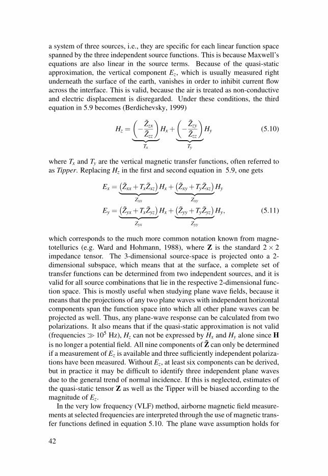
a system of three sources, i.e., they are specific for each linear function spacespanned by the three independent source functions. This is because Maxwell’sequations are also linear in the source terms. Because of the quasi-staticapproximation, the vertical component Ez, which is usually measured rightunderneath the surface of the earth, vanishes in order to inhibit current flowacross the interface. This is valid, because the air is treated as non-conductiveand electric displacement is disregarded. Under these conditions, the thirdequation in 5.9 becomes (Berdichevsky, 1999)

Hz =

(− Zzx

Zzz

)︸ ︷︷ ︸

Tx

Hx +

(−

Zzy

Zzz

)︸ ︷︷ ︸

Ty

Hy (5.10)

where Tx and Ty are the vertical magnetic transfer functions, often referred toas Tipper. Replacing Hz in the first and second equation in 5.9, one gets

Ex =(Zxx +TxZxz

)︸ ︷︷ ︸Zxx

Hx +(Zxy +TyZxz

)︸ ︷︷ ︸Zxy

Hy

Ey =(Zyx +TxZyz

)︸ ︷︷ ︸Zyx

Hx +(Zyy +TyZyz

)︸ ︷︷ ︸Zyy

Hy, (5.11)

which corresponds to the much more common notation known from magne-totellurics (e.g. Ward and Hohmann, 1988), where Z is the standard 2× 2impedance tensor. The 3-dimensional source-space is projected onto a 2-dimensional subspace, which means that at the surface, a complete set oftransfer functions can be determined from two independent sources, and it isvalid for all source combinations that lie in the respective 2-dimensional func-tion space. This is mostly useful when studying plane wave fields, because itmeans that the projections of any two plane waves with independent horizontalcomponents span the function space into which all other plane waves can beprojected as well. Thus, any plane-wave response can be calculated from twopolarizations. It also means that if the quasi-static approximation is not valid(frequencies 105 Hz), Hz can not be expressed by Hx and Hy alone since His no longer a potential field. All nine components of Z can only be determinedif a measurement of Ez is available and three sufficiently independent polariza-tions have been measured. Without Ez, at least six components can be derived,but in practice it may be difficult to identify three independent plane wavesdue to the general trend of normal incidence. If this is neglected, estimates ofthe quasi-static tensor Z as well as the Tipper will be biased according to themagnitude of Ez.

In the very low frequency (VLF) method, airborne magnetic field measure-ments at selected frequencies are interpreted through the use of magnetic trans-fer functions defined in equation 5.10. The plane wave assumption holds for

42

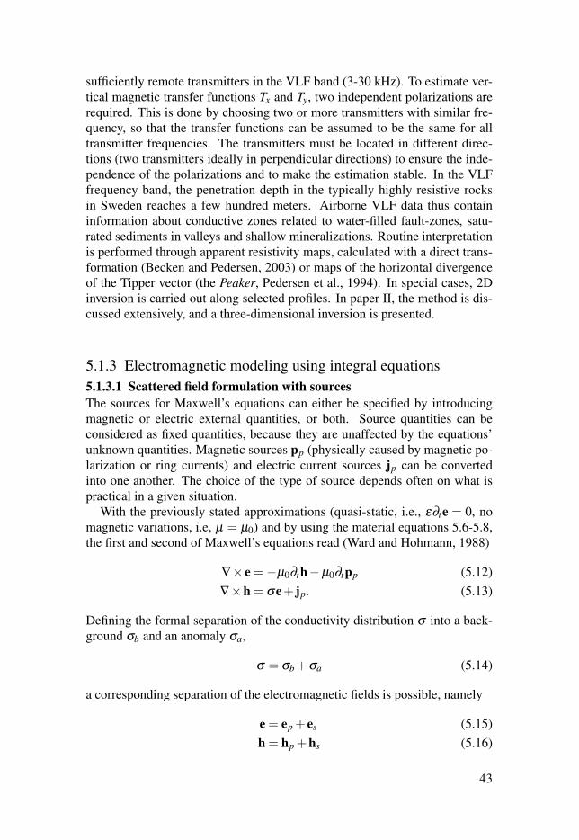
sufficiently remote transmitters in the VLF band (3-30 kHz). To estimate ver-tical magnetic transfer functions Tx and Ty, two independent polarizations arerequired. This is done by choosing two or more transmitters with similar fre-quency, so that the transfer functions can be assumed to be the same for alltransmitter frequencies. The transmitters must be located in different direc-tions (two transmitters ideally in perpendicular directions) to ensure the inde-pendence of the polarizations and to make the estimation stable. In the VLFfrequency band, the penetration depth in the typically highly resistive rocksin Sweden reaches a few hundred meters. Airborne VLF data thus containinformation about conductive zones related to water-filled fault-zones, satu-rated sediments in valleys and shallow mineralizations. Routine interpretationis performed through apparent resistivity maps, calculated with a direct trans-formation (Becken and Pedersen, 2003) or maps of the horizontal divergenceof the Tipper vector (the Peaker, Pedersen et al., 1994). In special cases, 2Dinversion is carried out along selected profiles. In paper II, the method is dis-cussed extensively, and a three-dimensional inversion is presented.

5.1.3 Electromagnetic modeling using integral equations5.1.3.1 Scattered field formulation with sourcesThe sources for Maxwell’s equations can either be specified by introducingmagnetic or electric external quantities, or both. Source quantities can beconsidered as fixed quantities, because they are unaffected by the equations’unknown quantities. Magnetic sources pp (physically caused by magnetic po-larization or ring currents) and electric current sources jp can be convertedinto one another. The choice of the type of source depends often on what ispractical in a given situation.

With the previously stated approximations (quasi-static, i.e., ε∂te = 0, nomagnetic variations, i.e, µ = µ0) and by using the material equations 5.6-5.8,the first and second of Maxwell’s equations read (Ward and Hohmann, 1988)

∇× e =−µ0∂th−µ0∂tpp (5.12)∇×h = σe+ jp. (5.13)

Defining the formal separation of the conductivity distribution σ into a back-ground σb and an anomaly σa,

σ = σb +σa (5.14)

a corresponding separation of the electromagnetic fields is possible, namely

e = ep + es (5.15)h = hp +hs (5.16)

43

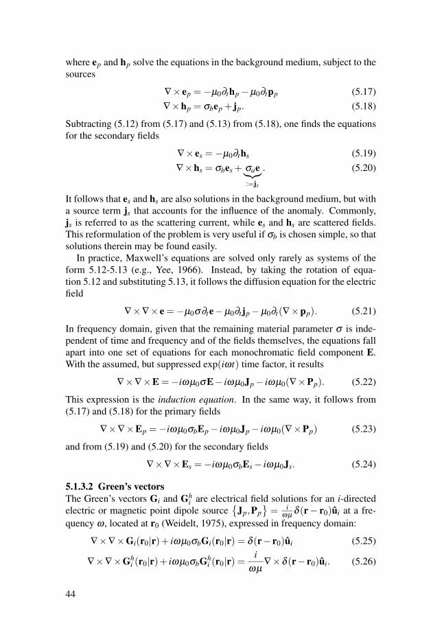
where ep and hp solve the equations in the background medium, subject to thesources

∇× ep =−µ0∂thp−µ0∂tpp (5.17)∇×hp = σbep + jp. (5.18)

Subtracting (5.12) from (5.17) and (5.13) from (5.18), one finds the equationsfor the secondary fields

∇× es =−µ0∂ths (5.19)∇×hs = σbes + σae︸︷︷︸

:=js

. (5.20)

It follows that es and hs are also solutions in the background medium, but witha source term js that accounts for the influence of the anomaly. Commonly,js is referred to as the scattering current, while es and hs are scattered fields.This reformulation of the problem is very useful if σb is chosen simple, so thatsolutions therein may be found easily.

In practice, Maxwell’s equations are solved only rarely as systems of theform 5.12-5.13 (e.g., Yee, 1966). Instead, by taking the rotation of equa-tion 5.12 and substituting 5.13, it follows the diffusion equation for the electricfield

∇×∇× e =−µ0σ∂te−µ0∂tjp−µ0∂t(∇×pp). (5.21)

In frequency domain, given that the remaining material parameter σ is inde-pendent of time and frequency and of the fields themselves, the equations fallapart into one set of equations for each monochromatic field component E.With the assumed, but suppressed exp(iωt) time factor, it results

∇×∇×E =−iωµ0σE− iωµ0Jp− iωµ0(∇×Pp). (5.22)

This expression is the induction equation. In the same way, it follows from(5.17) and (5.18) for the primary fields

∇×∇×Ep =−iωµ0σbEp− iωµ0Jp− iωµ0(∇×Pp) (5.23)

and from (5.19) and (5.20) for the secondary fields

∇×∇×Es =−iωµ0σbEs− iωµ0Js. (5.24)

5.1.3.2 Green’s vectorsThe Green’s vectors Gi and Gh

i are electrical field solutions for an i-directedelectric or magnetic point dipole source

Jp,Pp

= i

ωµδ (r− r0)ui at a fre-

quency ω , located at r0 (Weidelt, 1975), expressed in frequency domain:

∇×∇×Gi(r0|r)+ iωµ0σbGi(r0|r) = δ (r− r0)ui (5.25)

∇×∇×Ghi (r0|r)+ iωµ0σbGh

i (r0|r) =i

ωµ∇×δ (r− r0)ui. (5.26)

44

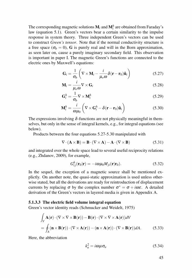
The corresponding magnetic solutions Mi and Mhi are obtained from Faraday’s

law (equation 5.1). Green’s vectors bear a certain similarity to the impulseresponse in system theory. Three independent Green’s vectors can be usedto construct Green’s tensor. Note that if the normal conductivity structure isa free space (σb = 0), G is purely real and will in the Born approximation,as seen later on, cause a purely imaginary secondary field. This observationis important in paper I. The magnetic Green’s functions are connected to theelectric ones by Maxwell’s equations:

Gi =1

σb

(∇×Mi−

iµoω

δ (r− r0)ui

)(5.27)

Mi =i

µoω∇×Gi (5.28)

Ghi =

1σb

∇×Mhi (5.29)

Mhi =

iωµ0

(∇×Gh

i −δ (r− r0)ui

)(5.30)

The expressions involving δ -functions are not physically meaningful in them-selves, but only in the sense of integral kernels, e.g., for integral equations (seebelow).

Products between the four equations 5.27-5.30 manipulated with

∇ · (A×B) = B · (∇×A)−A · (∇×B) (5.31)

and integrated over the whole space lead to several useful reciprocity relations(e.g., Zhdanov, 2009), for example,

Ghi j(r0|r) =−iωµ0M ji(r|r0). (5.32)

In the sequel, the exception of a magnetic source shall be mentioned ex-plictly. On another note, the quasi-static approximation is used unless other-wise stated, but all the derivations are ready for reintroduction of displacementcurrents by replacing σ by the complex number σ∗ = σ + iωε . A detailedderivation of the Green’s vectors in layered media is given in Appendix A.

5.1.3.3 The electric field volume integral equationGreen’s vector identity reads (Schmucker and Weidelt, 1975)∫

VA(r) · (∇×∇×B(r))−B(r) · (∇×∇×A(r))dV

=∮

A(n×B(r)) · (∇×A(r))− (n×A(r)) · (∇×B(r))dA. (5.33)

Here, the abbreviation

k2a = iωµσa (5.34)

45

is used. I specify a symmetric dot-product

A ·B = ∑i

AiBi (5.35)

as in paper II, but in contrast to the Hermitian dot-product used in paper I. If Bis chosen to be a Green’s vector Gi and A the secondary electric field Es, theright-hand side will vanish upon choosing an infinite integration volume. Thereason is that G and its surface integrals respectively, drop to zero at a fasterrate than the encompassing surface grows, given the location is far enoughaway from any sources. Using equations 5.24 and 5.25 to replace the ∇×∇×term, and in the end, using reciprocity, it follows∫

VEs(r) · (δ (r− r0)ui)+Gi(r0|r) ·

(k2

a(r)E(r))

dV = 0 (5.36)

and

Es(r0) · ui =− ∑j=x,y,z

∫V

G ji(r|r0) ·(k2

a(r)E(r) · u j)

dV. (5.37)

After re-introducting the primary field Ep, redefining r0 as the coordinate ofthe source and r the location of the field point and exchanging indices, thevolume integral equation is obtained. In terms of the field components, itreads

E j(r) = Ep, j(r)− ∑i=x,y,z

∫V0

Gi j(r0|r) ·(k2

a(r0)Ei(r0))

d3r0. (5.38)

The Born approximation

E j(r)≈ Ep, j(r)− ∑i=x,y,z

∫V0

Gi j(r0|r) ·(k2

a(r0)Ep,i(r0))

d3r0. (5.39)

is the basis of paper I.Electrodynamic modeling in paper II is carried out by solving equation 5.38.

Details are described in the paper. The main difficulty is that the discrete ver-sion of equation 5.38 yields a linear system of equations, where the systemmatrix has no zero elements (in contrast to finite difference or finite elementformulations, where the matrices are usually sparse). This makes it compu-tationally unwieldy and practically impossible to be factorized for a directsolution. It is therefore almost unavoidable to resort to an iterative solution ofthe forward problem. Consequently, the computation of Jacobian matrices foran inverse problem is infeasible because it requires numerous forward com-putations with the same system matrix. It is, however, advantageous that thedomain of discretization is identical with the anomalous domain, which in turnis equivalent to the domain of interest in an inverse problem.

Another noteworthy characteristic is that the system matrix is not complex-symmetric (see Appendix A), and thus requires dedicated iterative solvers suchas GMRES (Saad and Schultz, 1986) or BiCGstab (van der Vorst, 1992) in-stead of, for example, conjugate gradients (section 4.2.2).

46

5.1.4 The low-induction number approximation and the slingrammethod

In the quasi-static approximation, the penetration depth of plane waves is de-fined by the electromagnetic skin-depth

δ =

√2

ωµσ(5.40)

If δ is large compared to the induction volume, the low induction number ap-proximation can be applied. This is also denoted as the resistive limit (Grantand West, 1965). For example in the slingram method the receiver is located inthe near-field at a small distance s from the transmitter, where the field behav-ior is dominated by geometric damping. The induction number is accordinglydefined as s

δand if it is much smaller than unity, the low-induction-number

(LIN) approximation is indicated. The inducing magnetic field H is every-where practically without delay, so that it can be regarded static (apart fromthe time factor exp(iωt))(Landau and Lifšic, 1960). The electric field followsthen from Faraday’s law (equation 5.1), namely

∇×E =−iωµH (5.41)

which shows that the induced currents, and thus the secondary magnetic fieldsobtained from

∇×Hs = σE (5.42)

are directly proportional to the field frequency and lag behind in phase by π

2 .Many commonplace slingram instruments are designed to perform their mea-surements within the domain of the resistive limit, i.e., to use a frequency aslow as possible to minimize induction, but sufficiently high for the secondaryfield to be reliably detectable within the noise background. Through the phasedifference, it can be conveniently distinguished from the primary field and a di-rect reading of an apparent half-space conductivity value is available througha linear scaling of the induced quadrature voltage (McNeill, 1980). This isdiscussed in detail in paper I. There, this is illustrated by forming an integralequation like 5.38. By using an insulating background, i.e., σa =σ and σb = 0,Green’s tensor becomes real-valued. The phase shift and the proportionalityof the secondary field with frequency are introduced by the factor k2

a = iωµσa.The LIN approximation shows to be the Born approximation for the specialcase of an insulating background structure (compare equation 5.39).

5.1.5 Direct currentIn the dc geoelectric method, direct current is injected into the ground via twocurrent electrodes. The current distribution, determined by the conductivity

47

distribution in the subsurface, is investigated by measuring potential differ-ences between pairs of potential electrodes. For direct current, Maxwell’sequations simplify to

∇× e = 0 (5.43)∇×h = j+ jp. (5.44)

Taking the divergence of equation 5.44 and substituting j = σe, where e iswritten in terms of the scalar potential W as

e =−∇W, (5.45)

gives

∇ · (σ∇W ) = ∇ · jp. (5.46)

This is a Poisson equation for W . The potential can be found for each currentelectrode at a location r0 separately by setting

∇ · jp = Iδ (r− r0), (5.47)

where I denotes the source current. Equation 5.46 can be solved in variousways, e.g., in paper III, the 2.5D finite difference method following Dey andMorrison (1979) is used. The implementation has been provided by NaserMeqbel. It is described in Kalscheuer et al. (2010).

5.2 Refraction seismicsThe refraction seismic method is used in a variety of applications from near-surface to deep crustal studies. A review of shallow applications can be foundin Steeples (2000). A useful textbook with a detailed treatment of refractionseismics is for example Telford et al. (1990). The method can be used inregions where the seismic velocity increases monotonically with depth, a con-dition that is very often met, but with common exceptions. If the assumptionfails at least partially, there will be blind spots in the subsurface and the in-terpretation of the data can become erroneous. An additional source of erroroccurs when layers are too thin to appear as separate velocity branches in theseismogram, which is required to identify them (Gupta, 1977).

The measurements associated with the refraction seismic method are thearrival times of head waves or diving waves, comprising the earliest arrivaltimes in the seismogram, even though arrivals from such waves can also ap-pear at later times. The relevant phenomena can be described in terms of raytheory, only valid if the wave length is much smaller than the subsurface struc-tures. The path of the rays through the subsurface is determined by Fermat’sprinciple as the path of minimum travel time. Because the seismic velocity

48

almost always increases with depth, the ray paths dive into the subsurface toreach layers where faster propagation is possible. Both the transmission be-havior through interfaces and the ray curvature are dictated by Snell’s law,which locally defines the relationship between an incident and a transmittedwave at a (possibly infinitesimal) velocity contrast. For a piece-wise homoge-neous earth, the rays are piece-wise straight with sharp bends at the interfaces.At these interfaces, head waves can be generated under the following circum-stances: (1) The incoming wave approaches the interface through the mediumof lower velocity. (2) Its angle of incidence is large enough, so that the re-fracted wave, instead of propagating into the higher velocity medium, travelsalong the interface (critical refraction). From there, head waves emerge andcan reach the surface. Consequently, for a head wave, a sharp interface be-tween two media of different velocity is required. The original refracted wavetravels along the interface at the speed of the higher velocity medium. Hence,the associated head waves can be registered at large offsets from the source.In a gradually varying earth, the ray paths are curved and head waves do notoccur. In such a scenario, the early arrival times are dominated by smoothlybent rays from diving waves that return to the surface. Within the naturallyvarying velocity structure of the real earth, head waves are also subject to raybending.

A general method of calculating the travel times is through solution of theeikonal equation which comprises an arrival time field for one source in allspace (e.g., Zelt and Ellis, 1988). The ray path (eikonal) is required for thecalculation of the sensitivity with respect to the subsurface parameters. It isalways normal to contours of the travel time field and can be found by gradientdescent from the receiver to the transmitter.

The implementation used in this thesis is based on the two-dimensionalimplementation by Zelt and Ellis (1988). Therein, the layer interfaces are rep-resented by piece-wise linear functions. Each layer is constructed from severalhorizontally connected bi-linear velocity patches. Velocity discontinuities areonly possible across layer boundaries.

5.3 Potential fields5.3.1 GravityThe gravitational attraction g that is felt at a coordinate r due to a spatiallylimited massive body with a density distribution ρ(r) in its interior is given by

49

(Grant and West, 1965)

g(r) = γ∇

∫V

ρ(r0)

Rd3r0

=−γ

∫V

ρ(r0)r− r0

R3 d3r0

=−∇U(r)

R2 = (x− x0)2 +(y− y0)

2 +(z− z0)2 (5.48)

where γ is the gravitational constant and U is the gravitational potential

U(r) =−γ

∫V

ρ(r0)

Rd3r0. (5.49)

This is a direct consequence of Newton’s law of gravitation for point massesand the fact that in classical physics, gravitational fields are additive. Thecommonly measured quantity is the vertical component gz of g. For a ho-mogeneous, block-shaped body, a solution of the integral at the origin of thecoordinate system is (Sorokin, 1951; Li and Chouteau, 1998)

gz =−γρ

[[x log(y+ r)+ y log(x+ r)+ z tan−1(

zrxy

)]x2

x1

]y2

y1

z2

z1

r2 = x2 + y2 + z2. (5.50)

The block axes are aligned with the Cartesian coordinate axes and its spatialextent is x1 < x < x2, y1 < y < y2, z1 < z < z2.

5.3.2 MagneticsSimilar to the gravity field the anomalous magnetic field Ha due to magnet-ically anomalous bodies in the earth can be regarded as a potential field, be-cause in the absence of currents, Ampere’s law (equation 5.2) dictates that itis curl free. Consequently, Ha is representable by a scalar potential V (Grantand West, 1965; Blakely, 1995)

Ha(r) =−∇V (r) =1

4π∇

∫V

M(r0) ·∇1R

d3r0 (5.51)

where M is a spatially variable magnetic polarization vector. The potentialreads

V (r) =− 14π

∫V

M(r0) ·∇1R

d3r0. (5.52)

The magnetization is determined as

M = χH+MR (5.53)

50

where χ represents the magnetic susceptibility and H = Ha +H0 is the com-plete magnetic field intensity. The remanent magnetization is denoted by MR.Equations 5.51 and 5.53 result in the complicated integral equation

H(r) = (H0 +HR)+1

4π∇

∫V

χ(r0)H(r0) ·∇1R

d3r0. (5.54)

Here, HR is the magnetic field due to remanent magnetization as defined byequation 5.51 after substituting MR. Note that in free space and in the air half-space, the magnetic field intensity H and the magnetic induction B, i.e., thequantity which is accessible through measurement, only differ by the factor µ0(see material equation 5.7). A solution to the complete magnetostatic problemin the form of a differential equation has been implemented by Lelièvre andOldenburg (2006). In most practical applications, χ is small (|χ| 1) anddemagnetization effects may be neglected. The inducing field can then beregarded merely due to the homogeneous external magnetic field of the EarthH0 =

1µ0

B0, so that

M≈ χH0 +MR. (5.55)

Substituting the approximation 5.55 into equation 5.51 and adding H0 leads tothe Born approximation of equation 5.54, similar to the one discussed previ-ously in the electrodynamic context (equation 5.39). For this case, an explicitexpression for the anomaly of a block-shaped volume of homogeneous mag-netization similar to equation 5.50 exists. Commonly the total magnetic field∆T anomaly is measured and interpreted as the projection of the anomalousmagnetic field on the Earth’s main field B0. For this quantity the expression is(Bhattacharyya, 1964)

∆T =µ0

4π|M|

[[αyz log(

r− xr+ x

)+αxz log

(r− yr+ y

)−2αxy log(r+ z)

−αxx tan−1(

xyx2 + rz+ z2

)−αyy tan−1

(xy

r2 + rz− x2

)

+αzz tan−1(

xyrz

)]x2

x1

]y2

y1

z2

z1

αi j =12(eMieF j + eM jeFi) i, j = x,y,z

r2 = x2 + y2 + z2, (5.56)

where the induction direction (the direction of B0) is given by the unit vectoreF and the direction of magnetization is given by eM. Note that while the mag-nitude of the total field T = |B0+µHa| is measured and the quantity T −B0 is

51

interpreted as the total field anomaly ∆T , equation 5.56 actually calculates ∆Tas µ(Ha · eF), which is only equal to the former in the case of small anoma-lies (∆T < 0.2B0, Grant and West, 1965). In paper IV, an anomaly of roughly∆T ≈ 0.12B0 is observed, resulting in differences of locally up to 0.006B0between the simulation using equation 5.56 and a more accurate simulation,where the ∆T is derived from the anomalous field vector. This corresponds toabout 5% of the anomaly.

The remanent magnetization MR, if present, is often difficult to address. Inprinciple, it can only be distinguished from induced magnetization if it has asignificantly different direction. Attempts for determination of the vector mag-netization M or its amplitude (the total magnetization) via inversion of favor-ably transformed data or using a fixed magnetization direction were comparedand summarized by Li et al. (2010). An inversion method for spatially variablemagnetization magnitude and direction has been implemented by Lelièvre andOldenburg (2009).

5.3.3 Gravity gradiometryAnother quantity that is increasingly common to measure is the gravity gradi-ent tensor Γ (Pedersen and Rasmussen, 1990). It contains the spatial deriva-tives of g, i.e.,

Γ = ∇[gT ]=−∇

[(∇U)T ]

[Γ]i j =−∂i∂ jU = γ∂i∂ j

∫V

ρ(r0)

Rd3r0 (5.57)

Γ is symmetric and because outside of the body, the potential U fulfills theLaplace equation

∇2U = 0, (5.58)

it also has no trace, and thus it has five independent components. The relationbetween U and V is called Poisson’s relation. Compare equation 5.49 withequation 5.52 for equal volumes of homogeneous density and magnetizationto find

V =γ

4πρ(M ·∇U) . (5.59)

This relation serves as an important mathematical link between gravity andmagnetics. For magnetization along the unit vectors ex,y,z it follows

ex,y,z ·∇U =4πρ

γ|M|Vx,y,z (5.60)

and

[Γ]i j =−∂i (e j ·∇U) =− 4πρ

γ|M|∂iVj. (5.61)

52

Consequently, Γi j can be computed as ∆T with magnetization direction eM =

ei, field direction eF = e j and a magnetization magnitude of 4πγ

µ0ρ . Similar to

equations 5.56, the forward model becomes

(Γ)i j = γρ

[[αi jyz log

(r− xr+ x

)+α

i jxz log

(r− yr+ y

)−2α

i jxy log(r+ z)

−αi jxx tan−1

(xy

x2 + rz+ z2

)−α

i jyy tan−1

(xy

r2 + rz− x2

)

+αi jzz tan−1

(xyrz

)]x2

x1

]y2

y1

z2

z1

αi jkl =

12(δikδ jl +δilδ jk

)i, j,k, l = x,y,z. (5.62)

53

6. Summary of the papers

6.1 Inversion of slingram electromagnetic inductiondata using a Born approximation

Many slingram dual-loop systems are especially useful to the practitioner,since they provide a direct conductivity reading. Therefore, instruments ofthis kind are frequently used in, for example, environmental applications, hy-drogeophysics, engineering geophysics or archaeological prospection. Theconductivity reading relies on the validity of the low induction number (LIN)approximation. Because the approximation is linear in the conductivity, it hasalso been used for a convenient fast interpretation, even in three-dimensions(Pérez-Flores et al., 2012). However, for high frequencies and/or conductiv-ity, the approximation breaks down and the electromagnetic fields becomenon-linear in the conductivity, requiring a cumbersome rigorous modeling ofthree-dimensional electromagnetic fields (Sasaki and Meju, 2006).

In this paper, we present a low-effort compromise between the LIN approx-imation and rigorous modeling. We investigate the LIN approximation froman integral equation perspective and find that it is identical to a Born approx-imation in a free-space background structure. This generalization enables usto introduce background models that account for higher conductivity in thesubsurface by shifting the expansion point of the linearization, without requir-ing a non-linear computation. In particular, we use an arbitrarily conductivehomogeneous half-space background. Its conductivity value is readily cho-sen from the ensemble of apparent conductivity readings as an average of thetrue subsurface conductivity. The choice of a half-space is useful, becauseclosed-form expressions exist for the primary fields. Hence, all computationsare equally straight-forward for the corresponding Born approximation as theyare for the LIN approximation. The main difference is that the primary field isno longer purely real and the secondary field is no longer purely imaginary asit is the case when the background is insulating. By computing the imaginarypart of the shifted approximation, we can approximately simulate the apparentconductivity reading of the conductivity meter even where the LIN approxi-mation fails. The approximation is compared to rigorous 3D modeling. It isdemonstrated that conductive deviations from the background structure intro-duce a more severe mismatch than resistive deviations. We calculate improvedlinear kernels for two- and three-dimensional inversion that take all inductionwithin the conductive half-space background into account. With these ker-nels, we implement two- and three-dimensional inversions using a non-linearconjugate gradient technique.

54

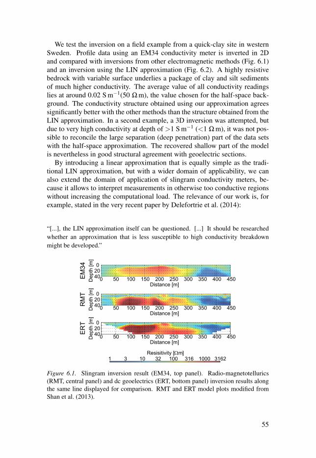
We test the inversion on a field example from a quick-clay site in westernSweden. Profile data using an EM34 conductivity meter is inverted in 2Dand compared with inversions from other electromagnetic methods (Fig. 6.1)and an inversion using the LIN approximation (Fig. 6.2). A highly resistivebedrock with variable surface underlies a package of clay and silt sedimentsof much higher conductivity. The average value of all conductivity readingslies at around 0.02 S m−1(50 Ω m), the value chosen for the half-space back-ground. The conductivity structure obtained using our approximation agreessignificantly better with the other methods than the structure obtained from theLIN approximation. In a second example, a 3D inversion was attempted, butdue to very high conductivity at depth of >1 S m−1 (<1 Ω m), it was not pos-sible to reconcile the large separation (deep penetration) part of the data setswith the half-space approximation. The recovered shallow part of the modelis nevertheless in good structural agreement with geoelectric sections.

By introducing a linear approximation that is equally simple as the tradi-tional LIN approximation, but with a wider domain of applicability, we canalso extend the domain of application of slingram conductivity meters, be-cause it allows to interpret measurements in otherwise too conductive regionswithout increasing the computational load. The relevance of our work is, forexample, stated in the very recent paper by Delefortrie et al. (2014):

“[...], the LIN approximation itself can be questioned. [...] It should be researchedwhether an approximation that is less susceptible to high conductivity breakdownmight be developed.”

0 50 100 150 200 250 300 350 400 450

0 20 40EM

34D

epth

[m]

Distance [m]

0 50 100 150 200 250 300 350 400 45040 20 0

RM

T

Distance [m]

Dep

th [m

]

0 50 100 150 200 250 300 350 400 45040 20 0

ER

T

Distance [m]

Dep

th [m

]

Resisitivity [ Ω m ] 1 3 10 32 100 316 1000 3162

Figure 6.1. Slingram inversion result (EM34, top panel). Radio-magnetotellurics(RMT, central panel) and dc geoelectrics (ERT, bottom panel) inversion results alongthe same line displayed for comparison. RMT and ERT model plots modified fromShan et al. (2013).

55

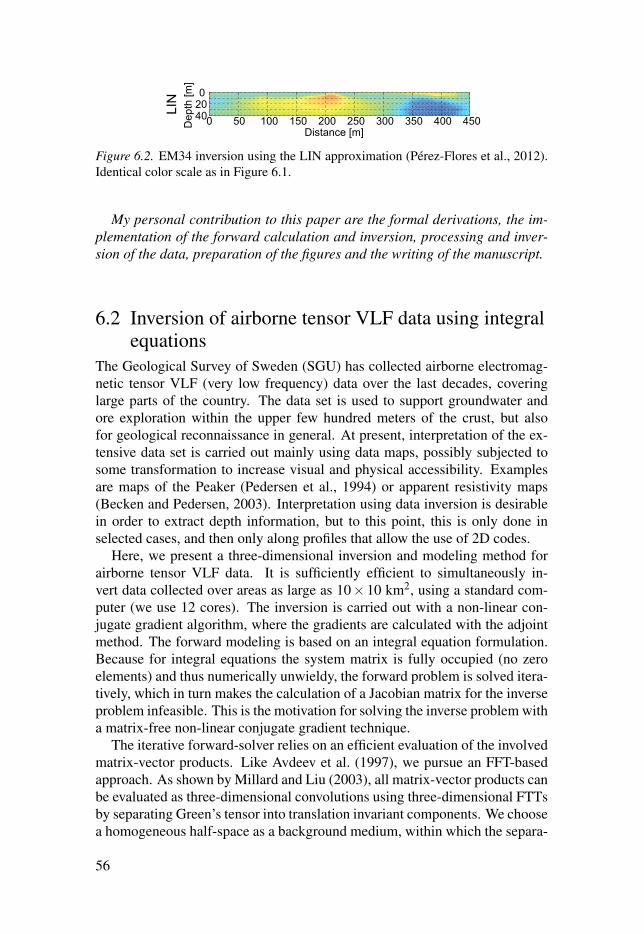
0 50 100 150 200 250 300 350 400 450

0 20 40LI

ND

epth

[m]

Distance [m]

Figure 6.2. EM34 inversion using the LIN approximation (Pérez-Flores et al., 2012).Identical color scale as in Figure 6.1.

My personal contribution to this paper are the formal derivations, the im-plementation of the forward calculation and inversion, processing and inver-sion of the data, preparation of the figures and the writing of the manuscript.

6.2 Inversion of airborne tensor VLF data using integralequations

The Geological Survey of Sweden (SGU) has collected airborne electromag-netic tensor VLF (very low frequency) data over the last decades, coveringlarge parts of the country. The data set is used to support groundwater andore exploration within the upper few hundred meters of the crust, but alsofor geological reconnaissance in general. At present, interpretation of the ex-tensive data set is carried out mainly using data maps, possibly subjected tosome transformation to increase visual and physical accessibility. Examplesare maps of the Peaker (Pedersen et al., 1994) or apparent resistivity maps(Becken and Pedersen, 2003). Interpretation using data inversion is desirablein order to extract depth information, but to this point, this is only done inselected cases, and then only along profiles that allow the use of 2D codes.

Here, we present a three-dimensional inversion and modeling method forairborne tensor VLF data. It is sufficiently efficient to simultaneously in-vert data collected over areas as large as 10× 10 km2, using a standard com-puter (we use 12 cores). The inversion is carried out with a non-linear con-jugate gradient algorithm, where the gradients are calculated with the adjointmethod. The forward modeling is based on an integral equation formulation.Because for integral equations the system matrix is fully occupied (no zeroelements) and thus numerically unwieldy, the forward problem is solved itera-tively, which in turn makes the calculation of a Jacobian matrix for the inverseproblem infeasible. This is the motivation for solving the inverse problem witha matrix-free non-linear conjugate gradient technique.

The iterative forward-solver relies on an efficient evaluation of the involvedmatrix-vector products. Like Avdeev et al. (1997), we pursue an FFT-basedapproach. As shown by Millard and Liu (2003), all matrix-vector products canbe evaluated as three-dimensional convolutions using three-dimensional FTTsby separating Green’s tensor into translation invariant components. We choosea homogeneous half-space as a background medium, within which the separa-

56

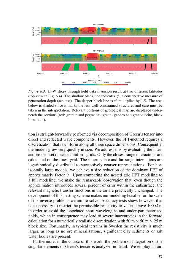
−400−200

0200

N = 7425550

Dep

th [m

]

1694000

−400−200

0200

E

N = 7424550

Dep

th [m

]

1684000 1686000 1688000 1690000 1692000

Resistivity [ Ωm] 100 316 1000 3162 10000 31623 100000

Figure 6.3. E–W slices through field data inversion result at two different latitudes(top view in Fig. 6.4). The shallow black line indicates , a conservative measure ofpenetration depth (see text). The deeper black line is multiplied by 1.5. The areabelow is shaded since it marks the less well-constrained structures and care must betaken in the interpretation. Relevant portions of geological map are displayed under-neath the sections (red: granite and pegmatite, green: gabbro and granodiorite, blackline: fault).

tion is straight-forwardly performed via decomposition of Green’s tensor intodirect and reflected wave components. However, the FFT-method requires adiscretization that is uniform along all three space dimensions. Consequently,the models grow very quickly in size. We address this by evaluating the inter-actions on a set of nested uniform grids. Only the closest range interactions arecalculated on the finest grid. The intermediate and far-range interactions arelogarithmically distributed to successively coarser representations. For hor-izontally large models, we achieve a size reduction of the dominant FFT ofapproximately factor 9. Upon comparing the nested grid FFT modeling toa full modeling, we make the remarkable observation that, even though theapproximation introduces several percent of error within the subsurface, therelevant magnetic transfer functions in the air are practically unchanged. Thedevelopment of this nesting scheme makes our modeling feasible for the scaleof the inverse problems we aim to solve. Accuracy tests show, however, thatis it necessary to restrict the permissible resistivity to values above 100 min order to avoid the associated short wavelengths and under-parameterizedfields, which in consequence may lead to severe inaccuracies in the forwardcalculation for a numerically realistic discretization with 50 m × 50 m × 25 mblock size. Fortunately, in typical terrains in Sweden the resistivity is muchlarger, as long as no ore mineralizations, significant clay sediments or saltwater bodies are present.

Furthermore, in the course of this work, the problem of integration of thesingular elements of Green’s tensor is analyzed in detail. We employ an an-

57

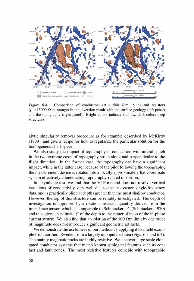
7421000

7423000

7425000

7427000

7429000

1684000 1686000 1688000 1690000 1692000

Fault zoneAlkaline GraniteGabbro, Diorite and Granodiorite

Granite Gabbro and Dolerite Granite and Pegmatite

7421000

7423000

7425000

7427000

7429000

1684000 1686000 1688000 1690000 1692000

Conductor depth [m], < 1500 m0 25 75 150 300 600

Resistor depth [m], > 15000 m0 25 75 150 300 600

3500

350

3500000

3500000005005000005000500500500503333

400440004044444444444400004000040000000004000040000000004

400000400444440000000000044

400 444444040404440440440444040404040440404444444444444444444444444444444444400

40000

40000404040

4444000000

4044000000404444444440000004044444444000000404040440040444

4000000000444040000004040440000000404044000000000000000044444

4000000000000000000000

4000000000000000000000000000000000000044

400004044 00000004044 0000004044 00000004

444444444444444444404040400000000000000000000000000000000000000

5455545450505045045450050505055005050500000444454545454545444445444444444444444544444445454545454545454545454545454

00005000505000055554545005050454544050504545450505500454544545444444444444444444444444444544545454545455545554550505050505050005000000000000000000

Figure 6.4. Comparison of conductors ( <1500 m, blue) and resistors( >15000 m, orange) in the inversion result with the surface geology (left panel)and the topography (right panel). Bright colors indicate shallow, dark colors deepstructures.

alytic singularity removal procedure as for example described by McKirdy(1989), and give a recipe for how to regularize the particular solution for thehomogeneous half-space.

We also study the impact of topography in connection with aircraft pitchin the two extreme cases of topography strike along and perpendicular to theflight direction. In the former case, the topography can have a significantimpact, while in the latter case, because of the pilot following the topography,the measurement device is rotated into a locally approximately flat coordinatesystem effectively counteracting topography-related distortion.

In a synthetic test, we find that the VLF method does not resolve verticalvariations of conductivity very well due to the in essence single-frequencydata, and is practically blind at depths greater than the most shallow conductor.However, the top of this structure can be reliably investigated. The depth ofinvestigation is appraised by a rotation invariant quantity derived from theimpedance tensor, which is comparable to Schmucker’s C (Schmucker, 1970)and thus gives an estimate of the depth to the center of mass of the in-phasecurrent system. We also find that a violation of the 100 m limit by one orderof magnitude does not introduce significant geometric artifacts.

We demonstrate the usefulness of our method by applying it to a field exam-ple from northern Sweden from a largely unpopulated area (Figs. 6.3 and 6.4).The mainly magmatic rocks are highly resistive. We uncover large scale elon-gated conductor systems that match known geological features such as con-tact and fault zones. The most resistive features coincide with topographic

58

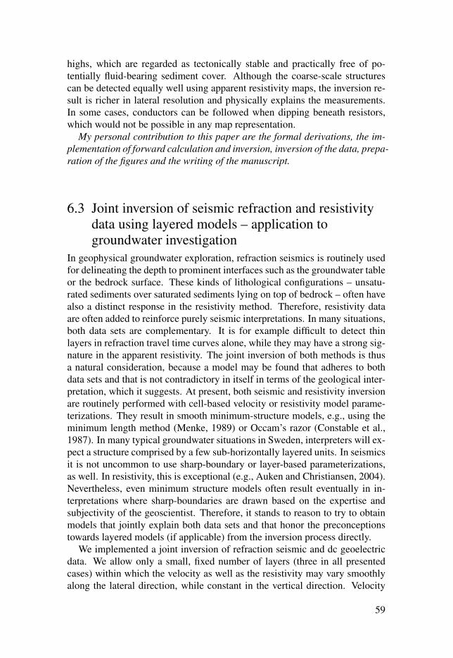
highs, which are regarded as tectonically stable and practically free of po-tentially fluid-bearing sediment cover. Although the coarse-scale structurescan be detected equally well using apparent resistivity maps, the inversion re-sult is richer in lateral resolution and physically explains the measurements.In some cases, conductors can be followed when dipping beneath resistors,which would not be possible in any map representation.

My personal contribution to this paper are the formal derivations, the im-plementation of forward calculation and inversion, inversion of the data, prepa-ration of the figures and the writing of the manuscript.

6.3 Joint inversion of seismic refraction and resistivitydata using layered models – application togroundwater investigation

In geophysical groundwater exploration, refraction seismics is routinely usedfor delineating the depth to prominent interfaces such as the groundwater tableor the bedrock surface. These kinds of lithological configurations – unsatu-rated sediments over saturated sediments lying on top of bedrock – often havealso a distinct response in the resistivity method. Therefore, resistivity dataare often added to reinforce purely seismic interpretations. In many situations,both data sets are complementary. It is for example difficult to detect thinlayers in refraction travel time curves alone, while they may have a strong sig-nature in the apparent resistivity. The joint inversion of both methods is thusa natural consideration, because a model may be found that adheres to bothdata sets and that is not contradictory in itself in terms of the geological inter-pretation, which it suggests. At present, both seismic and resistivity inversionare routinely performed with cell-based velocity or resistivity model parame-terizations. They result in smooth minimum-structure models, e.g., using theminimum length method (Menke, 1989) or Occam’s razor (Constable et al.,1987). In many typical groundwater situations in Sweden, interpreters will ex-pect a structure comprised by a few sub-horizontally layered units. In seismicsit is not uncommon to use sharp-boundary or layer-based parameterizations,as well. In resistivity, this is exceptional (e.g., Auken and Christiansen, 2004).Nevertheless, even minimum structure models often result eventually in in-terpretations where sharp-boundaries are drawn based on the expertise andsubjectivity of the geoscientist. Therefore, it stands to reason to try to obtainmodels that jointly explain both data sets and that honor the preconceptionstowards layered models (if applicable) from the inversion process directly.

We implemented a joint inversion of refraction seismic and dc geoelectricdata. We allow only a small, fixed number of layers (three in all presentedcases) within which the velocity as well as the resistivity may vary smoothlyalong the lateral direction, while constant in the vertical direction. Velocity

59

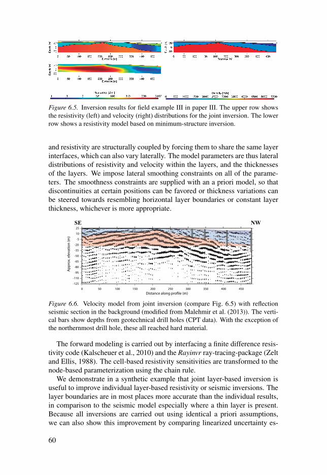
Figure 6.5. Inversion results for field example III in paper III. The upper row showsthe resistivity (left) and velocity (right) distributions for the joint inversion. The lowerrow shows a resistivity model based on minimum-structure inversion.

and resistivity are structurally coupled by forcing them to share the same layerinterfaces, which can also vary laterally. The model parameters are thus lateraldistributions of resistivity and velocity within the layers, and the thicknessesof the layers. We impose lateral smoothing constraints on all of the parame-ters. The smoothness constraints are supplied with an a priori model, so thatdiscontinuities at certain positions can be favored or thickness variations canbe steered towards resembling horizontal layer boundaries or constant layerthickness, whichever is more appropriate.

SE NW

App

rox.

ele

vatio

n (m

)

25

10

-5

-20

-35

-50

-65

-80

-95

-110

-125

0 50 100 150 200 250 300 350 400 450

Figure 6.6. Velocity model from joint inversion (compare Fig. 6.5) with reflectionseismic section in the background (modified from Malehmir et al. (2013)). The verti-cal bars show depths from geotechnical drill holes (CPT data). With the exception ofthe northernmost drill hole, these all reached hard material.

The forward modeling is carried out by interfacing a finite difference resis-tivity code (Kalscheuer et al., 2010) and the Rayinvr ray-tracing-package (Zeltand Ellis, 1988). The cell-based resistivity sensitivities are transformed to thenode-based parameterization using the chain rule.

We demonstrate in a synthetic example that joint layer-based inversion isuseful to improve individual layer-based resistivity or seismic inversions. Thelayer boundaries are in most places more accurate than the individual results,in comparison to the seismic model especially where a thin layer is present.Because all inversions are carried out using identical a priori assumptions,we can also show this improvement by comparing linearized uncertainty es-

60

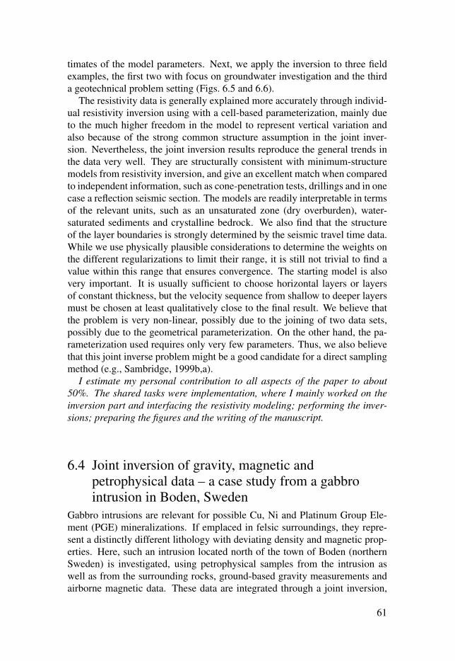
timates of the model parameters. Next, we apply the inversion to three fieldexamples, the first two with focus on groundwater investigation and the thirda geotechnical problem setting (Figs. 6.5 and 6.6).

The resistivity data is generally explained more accurately through individ-ual resistivity inversion using with a cell-based parameterization, mainly dueto the much higher freedom in the model to represent vertical variation andalso because of the strong common structure assumption in the joint inver-sion. Nevertheless, the joint inversion results reproduce the general trends inthe data very well. They are structurally consistent with minimum-structuremodels from resistivity inversion, and give an excellent match when comparedto independent information, such as cone-penetration tests, drillings and in onecase a reflection seismic section. The models are readily interpretable in termsof the relevant units, such as an unsaturated zone (dry overburden), water-saturated sediments and crystalline bedrock. We also find that the structureof the layer boundaries is strongly determined by the seismic travel time data.While we use physically plausible considerations to determine the weights onthe different regularizations to limit their range, it is still not trivial to find avalue within this range that ensures convergence. The starting model is alsovery important. It is usually sufficient to choose horizontal layers or layersof constant thickness, but the velocity sequence from shallow to deeper layersmust be chosen at least qualitatively close to the final result. We believe thatthe problem is very non-linear, possibly due to the joining of two data sets,possibly due to the geometrical parameterization. On the other hand, the pa-rameterization used requires only very few parameters. Thus, we also believethat this joint inverse problem might be a good candidate for a direct samplingmethod (e.g., Sambridge, 1999b,a).

I estimate my personal contribution to all aspects of the paper to about50%. The shared tasks were implementation, where I mainly worked on theinversion part and interfacing the resistivity modeling; performing the inver-sions; preparing the figures and the writing of the manuscript.

6.4 Joint inversion of gravity, magnetic andpetrophysical data – a case study from a gabbrointrusion in Boden, Sweden

Gabbro intrusions are relevant for possible Cu, Ni and Platinum Group Ele-ment (PGE) mineralizations. If emplaced in felsic surroundings, they repre-sent a distinctly different lithology with deviating density and magnetic prop-erties. Here, such an intrusion located north of the town of Boden (northernSweden) is investigated, using petrophysical samples from the intrusion aswell as from the surrounding rocks, ground-based gravity measurements andairborne magnetic data. These data are integrated through a joint inversion,

61

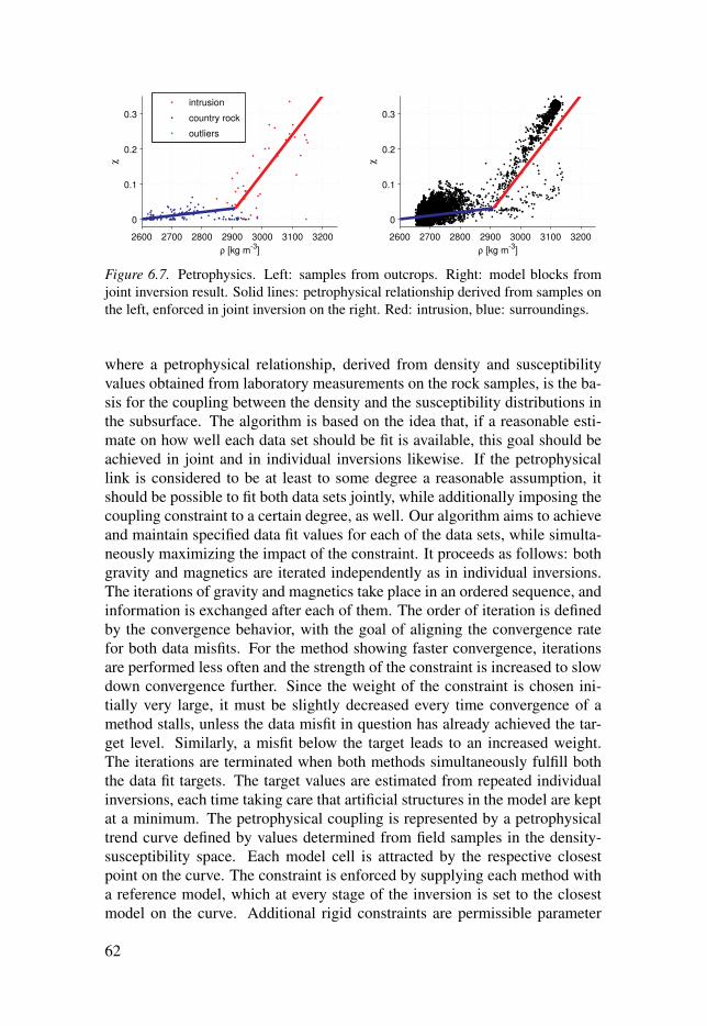
2600 2700 2800 2900 3000 3100 3200

0

0.1

0.2

0.3

χ

ρ [kg m-3

]

2600 2700 2800 2900 3000 3100 3200

0

0.1

0.2

0.3χ

ρ [kg m-3

]

intrusion

country rock

outliers

Figure 6.7. Petrophysics. Left: samples from outcrops. Right: model blocks fromjoint inversion result. Solid lines: petrophysical relationship derived from samples onthe left, enforced in joint inversion on the right. Red: intrusion, blue: surroundings.

where a petrophysical relationship, derived from density and susceptibilityvalues obtained from laboratory measurements on the rock samples, is the ba-sis for the coupling between the density and the susceptibility distributions inthe subsurface. The algorithm is based on the idea that, if a reasonable esti-mate on how well each data set should be fit is available, this goal should beachieved in joint and in individual inversions likewise. If the petrophysicallink is considered to be at least to some degree a reasonable assumption, itshould be possible to fit both data sets jointly, while additionally imposing thecoupling constraint to a certain degree, as well. Our algorithm aims to achieveand maintain specified data fit values for each of the data sets, while simulta-neously maximizing the impact of the constraint. It proceeds as follows: bothgravity and magnetics are iterated independently as in individual inversions.The iterations of gravity and magnetics take place in an ordered sequence, andinformation is exchanged after each of them. The order of iteration is definedby the convergence behavior, with the goal of aligning the convergence ratefor both data misfits. For the method showing faster convergence, iterationsare performed less often and the strength of the constraint is increased to slowdown convergence further. Since the weight of the constraint is chosen ini-tially very large, it must be slightly decreased every time convergence of amethod stalls, unless the data misfit in question has already achieved the tar-get level. Similarly, a misfit below the target leads to an increased weight.The iterations are terminated when both methods simultaneously fulfill boththe data fit targets. The target values are estimated from repeated individualinversions, each time taking care that artificial structures in the model are keptat a minimum. The petrophysical coupling is represented by a petrophysicaltrend curve defined by values determined from field samples in the density-susceptibility space. Each model cell is attracted by the respective closestpoint on the curve. The constraint is enforced by supplying each method witha reference model, which at every stage of the inversion is set to the closestmodel on the curve. Additional rigid constraints are permissible parameter

62

Density contrast [kg/m3]

2700 2800 2900 3000 3100 Susceptibility

0 0.1 0.2 0.3 Susceptibility

0 0.1 0.2 0.3

Figure 6.8. Joint inversion result, paper IV, left: density model, right: susceptibilitymodel. In the central and eastern part, cells with density values >2900 kg m−3 orsusceptibility values >0.1 are shown to delimit the intrusion. In the western part allmodel cells are displayed to illustrate the background structure.

intervals derived from the petrophysical data, which are enforced through alogarithmic parameter transform.

The joint inversion algorithm is investigated using a synthetic model sim-ilar to the field case. Performance of joint against individual inversion isevaluated through comparison of results using otherwise identical conditions.We find that the joint inversion improves the distinction between the back-ground medium and the intrusion through a much sharper contrast and gen-erally larger, more correct amplitudes in the anomalous body. Neither of theinversions can, however, reliably reproduce the lower boundary of the intru-sion, its near-surface zone or complex geometry at depth. This result demon-strates the typical non-uniqueness in potential field data and shows that thejoint inversion by itself can at best alleviate the problem.

The joint inversion result for the field example is correspondent to the syn-thetic inversion results. The petrophysical constraint is successfully enforced(Fig. 6.7), which leads to a geometric match of the density and susceptibilitymodels (Fig. 6.8). The resulting 3D model satisfactorily explains both fielddata sets and is in accordance with the petrophysical samples. Because of thesharp contrast between the lithological units, which spatially coincides in bothdensity and susceptibility, a geometrically consistent interpretation is easilyderived. The estimated geometry of the intrusion is clear and simple. Theinversion result is therefore a useful candidate model that can be tested andrefined.

We also discuss depth weighting-constraints introduced through weightedparameter damping. As proposed by Li and Oldenburg (1996, 1998), thedepth-weighting is supposed to emulate the square root of the depth-decayof the sensitivity kernel. We add a new theoretical argument to this, showingthat for a simple linear one-measurement problem the corresponding general-

63

ized inverse matrix is constant in magnitude for such a choice of weightingand thus produces a constant magnitude model. We argue that non-uniquenessin this simple case is similar to the non-uniqueness in the 3D potential fieldinversion problem.

In this paper, I designed and implemented and performed the joint and in-dividual inversions. I also implemented the forward codes, prepared most ofthe figures and wrote large parts of the manuscript (about 85%).

64

7. Discussion and conclusions

In this thesis, many different aspects of inversion and of the required forwardcalculations were investigated. The conclusions drawn are listed in the follow-ing.

In paper I, the dual loop electromagnetic induction problem is solved usinga novel approximation – a Born approximation around a homogeneous half-space background. In cases where the conductivity is not to be neglected butnot too inhomogeneous, the approximation can be applied and yields moreaccurate results than the standard LIN approximation without making the in-version more expensive. Especially larger loop separation data are prone tosensing a higher amount of inhomogeneity within the ground because of thelarger induction volume, and are thus often more difficult to treat in an approx-imate sense.

In paper II, a rigorous three-dimensional inversion of airborne VLF datahas been implemented using an integral equation approach within a non-linearconjugate gradient inversion. The forward modeling is expensive becauseof the high frequency in relation to the scale of the model. However, sincethe measurement locations lie in the air half-space, and because large wave-number errors vanish during field propagation, computational accuracy withinthe subsurface is of limited consequence. Hence, it is possible to save re-sources through the use of an approximate solution of the integral equation.This is achieved through an approximation of the convolutions by performingthe FFTs on nested grids. The inversion improves map-based interpretationprimarily by emphasizing lateral contrasts. Conducted synthetic experimentsand sensitivity studies show that the resolution of single frequency VLF trans-fer functions along the vertical axis is limited by the depth of the shallowestconductor. The depth variation of the top of this structure can be investigated.

In paper III, the practically relevant joint inversion problem of dc geoelec-tric and refraction seismic has been approached with layered models. In manynear-surface applications, a laterally variable layered earth is a good image ofthe geology, and such an image can be directly recovered through the use ofthe corresponding parameterization. Furthermore, the joint inversion aspectensures that multiple data sets can be inverted in order to yield a single, con-sistent model. This works well where the layer assumption for velocity andresistivity is valid, but otherwise layer interfaces may be misleading. The re-stricted freedom in the vertical direction compared to cell-based models leadsto larger data misfits in many cases.

In paper IV, a joint inversion algorithm is applied to gravity and magneticdata from a gabbroic intrusion, successfully integrating data from a large field

65

sampling campaign. It is demonstrated that joint inversion can lead to greatlyimproved results when appropriate a priori information is included. Addition-ally the importance of avoiding an unbalanced data fit between both involveddata sets shows, as it reduces ambiguity on the upper bound for the strengthof the model coupling constraint. The typical square root depth weighting isdiscussed under the light of the generalized inverse of a simple proxy problem,providing an additional justification for it.

In this thesis, the effectiveness of well-established simple conjugate gra-dient methods for solving problems that are at present computationally chal-lenging is confirmed (papers I, II, IV). In many cases, forward models do notrequire extreme accuracy (papers I, II), which allows to conserve computa-tional resources. Model appraisal is generally difficult within the proposedinverse schemes. In the presented field examples, the accuracy of the resultsis assessed either through synthetic studies (paper II, IV, III), sensitivity (pa-per II) or independent information (papers I, III), the latter not always beingavailable. Joint inversion helps to harmonize disparate data sets with consis-tent models, thus increasing their usefulness to the interpreting geoscientist.Care must be taken, however, when choosing the model coupling assump-tions. The layered-model assumption (paper III) may be useful in sedimentaryenvironments. Petrophysical coupling is only feasible if a representative set ofsamples is available (paper IV).

The presented inverse problems, although mathematically sufficiently sim-ilar to be implemented in one single code framework, behave differently interms of convergence, non-uniqueness, effectiveness of different regulariza-tions, and obviously in scale. The problem with the largest scale in this thesisis the potential field inversion presented in paper IV. This problem showedalso the best convergence behavior (due to the linearity of the forward oper-ator) and the highest degree of flexibility in the solution to accommodate forjoint inversion model coupling or other constraints. Both is due to the inher-ent non-uniqueness of potential field data. The inverse problem discussed inpaper I shows a high degree of uniqueness despite the linear approximation.Although computationally the most challenging problem, the airborne VLF in-version (paper II) is well-behaved in the sense that a model can be found onlyafter very few conjugate gradient iterations. This is because of the relativelylimited information content in this data due to the limited frequency range.The problem with the highest degree of non-linearity in this thesis is the jointinversion problem in paper III, presumably because of the layer-based modelparameterization and because a seismic method is involved. The problem ismore difficult to control than the other problems in this thesis. This manifestsitself in a much more complicated regularization procedure.

66

8. Acknowledgments

It is my honor to thank all the people who helped me in making my researchsuccessful:

I would like to express my gratitude to my supervisor Laust Pedersen. Hehas been an excellent guide throughout. He gave me the largest freedom topursue whatever I found interesting, whilst exerting guidance through sparkingmy interest during our countless inspiring discussions. Trying to live up toLaust’s unbroken confidence in my judgment unsurprisingly turned out to myadvantage, to my personal and scientific growth. What I appreciate most is thatregardless of the circumstances, he never failed to be present and supportive.

I am indebted to my second supervisor Mehrdad Bastani, who always be-lieved in me, who has invested a lot of time in discussions within which alarge number of creative ideas were born. Mehrdad made me feel very wel-come here in Uppsala, as the kind and warm person who he is. Mehrdad alsowas unbelievably diligent in covering my back and giving me time for mystudies.

I would like to thank Ari Tryggvason. He was my third supervisor andlater even accepted the risk of taking over my supervisor-ship completely. Healways provided good advice and helped in checking the manuscripts.

My gratitude goes to Michael Becken, who before all this began suggestedto me to apply to Laust. During January and February 2012, he also hostedme in Münster for several weeks and gave me a lot of supervision during thedevelopment of the integral inversion modeling, which later lead to papers Iand II. (Pure irony that the winter I spent there has been the coldest winter ofthese 5 years.)

Out of the listed people, Laust, Mehrdad and Michael have been workingwith me on authoring the manuscripts, as have Niklas Juhojuntti, Ildikó An-tal Lundin and Martiya Sadeghi from SGU. I very much enjoyed the smoothcooperation.

I would like to thank Chunling Shan for helping with the collection of theEM34 data in Lilla Edet under very challenging weather conditions.

Gratitude also goes to the cooperators from Sintef and NGU for the pleasantatmosphere in our project work and for having me in Trondheim for one weekto discuss programming and joint inversion.

In the assembly of this thesis, some people were very helpful. These wereforemost my supervisors, Ester?, Niklas and Peter, who each supplied me withmany comments and suggestions. Ester made a great difference to the quality

67

of numerous illustrations. Niklas helped me with the Swedish summary. Ad-ditional help with last minute corrections came from Maria, Thomas, Michaeland Steffi.

Thanks to Michael, Maria, Peter and Arnaud for saving me from the com-puter apocalypse.

Many thanks to Anna and Chris for giving me shelter during my first twomonths in Uppsala and for fixing my bike throughout. Thanks to Sofie forhaving a place to stay for me during my visit of Sintef in Trondheim.

Thank you everybody in Geocentrum, for making this place such a goodworking environment.

Cheers to all friends I made during those years, to my friends I left behind,to my family and to Ester. Without you, it would not have been worth it!

? yes, that’s a star!

68

References

Abubakar, A., M. Li, G. Pan, J. Liu, and T. M. Habashy (2011). Joint MT and CSEMdata inversion using a multiplicative cost function approach. Geophysics 76(3),F203–F214.

Aster, R. C., B. Borchers, and C. H. Thurber (2005). Parameter estimation andinverse problems. San Diego, CA: Academic Press.

Auken, E. and A. V. Christiansen (2004). Layered and laterally constrained 2Dinversion of resistivity data. Geophysics 69, 752–761.

Avdeev, Dmitry, B., A. V. Kuvshinov, O. V. Pankratov, and G. A. Newman (1997).High-performance three-dimensonal electromagnetic modelling using modifiedNeumann series. Wide-band numerical solution and examples. J. Geomagn.Geoelec. 49, 1519–1539.

Backus, G. and F. Gilbert (1968). The resolving power of gross earth data. Geophys.J. R. Astron. Soc. 16, 169–205.

Backus, G. and F. Gilbert (1970). Uniqueness in the inversion of inaccurate grossearth data. Philos. Trans. R. Soc. London, Ser. A 266, 123–192.

Becken, M. and L. B. Pedersen (2003). Transformation of vlf anomaly maps intoapparent resistivity and phase. Geophysics 68(2), 497–505.

Berdichevsky, M. N. (1999). Marginal notes on magnetotellurics. Surv.Geophys 20(3–4), 341–375.

Bhattacharyya, B. K. (1964). Magnetic anomalies due to prism-shaped bodies witharbitrary polarization. Geophysics 29(4), 517–531.

Blakely, R. J. (1995). Potential Theory in Gravity & Magnetic Applications.Melbourne, Australia: Cambridge University Press.

Christensen, N. B. (1990, JUL). Optimized fast Hankel transform filters. Geophys.Prospect. 38(5), 545–568.

Cole, K. S. and R. H. Cole (1941). Dispersion and absorption in dielectrics I.Alternating current characteristics. J. Chem. Phys. 9(4), 341–351.

Constable, S. C., R. L. Parker, and C. G. Constable (1987). Occam’s inversion: apractical algorithm for generating smooth models from electromagnetic soundingdata. Geophysics 52(3), 289–300.

Cox, L. H., G. A. Wilson, and M. S. Zhdanov (2010). 3D inversion of airborneelectromagnetic data using a moving footprint. Explor. Geophys. 41(4), 250–259.

Delefortrie, S., T. Saey, E. Van De Vijver, P. De Smedt, T. Missiaen, I. Demerre, andM. Van Meirvenne (2014). Frequency domain electromagnetic induction survey inthe intertidal zone: Limitations of low-induction-number and depth of exploration.J. Appl. Geophys. 100, 14–22.

Dey, A. and H. F. Morrison (1979). Resistivity modeling for arbitrarily shaped2-dimensional structures. Geophys. Prospect. 27(1), 106–136.

Eckel, B. (2000). Thinking in C++: Introduction to Standard C++, Volume One.Thinking in C++. Prentice Hall.

69

Egbert, G. D. and A. Kelbert (2012). Computational recipes for electromagnicinverse problems. Geophys. J. Int. 189, 251–267.

Ellis, R. G. and D. W. Oldenburg (1994). Applied geophysical inversion. Geophys. J.Int. 116, 5–11.

Fletcher, R. and C. M. Reeves (1964). Function minimization by conjugate gradients.Computer Journal 7, 149–154.

Gallardo, L. A. and M. Meju (2003). Characterization of heterogeneous near-surfacematerials by joint 2D inversion of dc and seismic data. Geophys. Res. Lett. 30(13),L1658.

Gao, G., A. A., and T. M. Habashy (2012). Joint petrophysical inversion ofelectromagnetic and full-waveform seismic data. Geophysics 77(3), WA3–WA18.

Gao, G. and Torres-Verdín (2005). Analytical techniques to evaluate the integrals of3D and 2D spatial dyadic Green’s functions. Prog. Electromagn. Res 52, 47–80.

Gauss, C. F. (1809). Theoria motus corporum coelestium in sectionibus conicissolem ambientium. Hamburg, Germany: F. Perthes und I. H. Besser.

Golub, G. H. and D. P. O’Leary (1989). Some history of the conjugate gradient andLanczos algorithms: 1948–1976. SIAM Review 31(1), 50–102.

Gradshteyn, I. S. and I. M. Ryzhik (2000). Table of Integrals, Series, and Products(Sixth ed.). San Diego, CA: Academic Press. translated from the Russian.

Grant, F. S. and G. F. West (1965). Interpretation Theory in Applied Geophysics(First ed.). McGraw-Hill, Inc.

Grayver, A. V., R. Streich, and O. Ritter (2013, JUN). Three-dimensional paralleldistributed inversion of CSEM data using a direct forward solver. Geophys. J.Int. 193(3), 1432–1446.

Gupta, S. (1977). Hidden layer problem in seismic refraction work. Geophys.Prospect. 25, 385–387.

Haber, E. and M. Holtzman Gazit (2013). Model fusion and joint inversion. Surv.Geophys 34, 675–695.

Haber, E. and D. W. Oldenburg (1997). Joint inversion: a structural approach.Inverse Prob. 13, 63–77.

Heincke, B., M. Jegen, M. Moorkamp, J. Chen, and R. W. Hobbs (2010). Adaptivecoupling strategy for simultaneous joint inversion that use petrophysicalinformation as constraints. SEG Technical Program Expanded Abstracts 550,2805–2809.

Hohmann, G. W. (1975). Three-dimensional induced polarization andelectromagnetic modeling. Geophysics 40(2), 309–324.

Kalscheuer, T., M. García Juanetey, N. Meqbel, and L. B. Pedersen (2010).Non-linear model error and resolution properties from two-dimensional single andjoint inversions of direct current resistivity and radiomagnetotelluric data.Geophys. J. Int. 182, 1174–1188.

Kalscheuer, T., J. Hübert, A. Kuvshinov, L. T., and L. B. Pedersen (2012). A hybridregularization scheme for the inversion of magnetotelluric data from natural andcontrolled sources to layer and distortion parameters. Geophysics 77(4),E301–E315.

Kozlovskaya, E., L. Vecsey, J. Plomerová, and T. Raita (2007). Joint inversion ofmultiple data types with the use of multiobjective optimization: problemformulation and application to the seismic anisotropy investigations. Geophys. J.

70

Int. 171(2), 76–779.Landau, L. D. and E. M. Lifšic (1960). Electrodynamics of continuous media,

Volume 8 of Course of theoretical physics. Pergamon, Oxford.Legendre, A. M. (1805). Nouvelles Méthodes pour la détermination des orbites des

Comètes, Chapter Sur la Méthode des moindres quarrés, pp. 72–80. Paris, France:Courcier.

Lelièvre, P. G., C. G. Farquharson, and A. C. Hurich (2012). Joint inversion ofseismic traveltimes and gravity data on unstructured grids with application tomineral exploration. Geophysics 77(1), K1–K15.

Lelièvre, P. G. and D. W. Oldenburg (2006). Magnetic forward modelling andinversion for high susceptibility. Geophys. J. Int. 166, 76–90.

Lelièvre, P. G. and D. W. Oldenburg (2009). A 3D total magnetization inversionapplicable when significant, complicated remanence is present. Geophysics 74(3),L21–L30.

Levenberg, K. (1944). A method for the solution of certain non-linear problems inleast squares. Quarterly of Applied Mathematics 2, 164–168.

Li, X. and M. Chouteau (1998). Three-dimensional gravity modeling in all space.Surv. Geophys 19, 339–368.

Li, Y. and D. W. Oldenburg (1996). 3-D inversion of magnetic data.Geophysics 61(2), 394–408.

Li, Y. and D. W. Oldenburg (1998). 3D inversion of gravity data. Geophysics 63,109–119.

Li, Y., S. E. Shearer, M. M. Haney, and N. Dannemiller (2010). Comprehensiveapproaches to 3D inversion of magnetic data affected by remanent magnetization.Geophysics 75(1), L1–L11.

Lines, L., A. K. Schultz, and S. Treitel (1988). Cooperative inversion of geophysicaldata. Geophysics 53(1), 8–20.

Loris, I., G. Nolet, I. Daubechies, and F. A. Dahlen (2007). tomographic inversionusing l(1)-norm regularization of wavelet coefficients. Geophys. J. Int. 170(1),359–370.

Mackie, R. L. and T. R. Madden (1993). 3-Dimensional magnetotelluric inversionusing conjugate gradients. Geophys. J. Int. 115(1), 215–229.

Malehmir, A., M. Saleem, and M. Bastani (2013). High-resolution reflectionseismics investigations of quick-clay and associated formations at a landslide scarin southwest sweden. J. Appl. Geophys. 92, 84–102.

Marler, R. T. and J. S. Arora (2004). Survey of multi-objective optimization methodsfor engineering. Struct. Multidisc. Optim. 26, 369–395.

Marquardt, D. (1963). An algorithm for least-squares estimation of nonlinearparameters. SIAM J. Appl. Math. 11(2), 431–441.

McGillivray, P. R. and D. W. Oldenburg (1990). Methods for calculating Fréchetderivatives and sensitivities for the non-linear inverse problem: a comparativestudy. Geophys. Prospect. 38, 499–524.

McKirdy, D. M. (1989). Recent improvements to the application of the volumeintegral method of eddy current modeling. J. Nondestr. Eval. 8(1), 45–52.

McNeill, J. D. (1980). Electromagnetic terrain conductivity measurement at lowinduction numbers. Technical Note TN6, Geonics Ltd.

71

Menke, W. (1989). Geophysical data analysis: discrete inverse theory (Revised ed.),Volume 45 of International Geophysics Series. Academic Press.

Millard, X. and Q. H. Liu (2003). A fast volume integral equation solver forelectromagnetic scattering from large inhomogeneous objects in planarly layeredmedia. IEEE Trans. Antennas Propag. 51(9), 2393–2401.

Molodtsov, D. M., V. N. Troyan, Y. V. Roslov, and A. Zerilli (2013). Joint inversionof seismic traveltimes and magnetotelluric data with a directed structuralconstraint. Geophysics 61, 1218–1228.

Moorkamp, M., B. Heincke, M. Jegen, A. W. Roberts, and R. W. Hobbs (2011). Aframework for 3-D joint inversion of MT, gravity and seismic refraction data.Geophysical Journal International 184, 477–493.

Newman, G. A. and D. L. Alumbaugh (2000). Three-dimensional magnetotelluricinversion using non-linear conjugate gradients. Geophys. J. Int. 140, 410–424.

Newman, G. A. and G. M. Hoversten (2000). Solution strategies for two- andthree-dimensional electromagnetic inverse problems. Inverse Prob. 16,1357–1375.

Nocedal, J. and S. J. Wright (2006). Numerical optimization (Second ed.). Berlin,Germany: Springer.

Oldenburg, D. W. (1978). Joint inversion of magnetotelluric and direct-currentresistivity measurements. Geophysics 43, 610–625.

Oldenburg, D. W. and Y. Li (2005). Inversion for applied geophysics: A tutorial,Chapter 5, pp. 89–150. Number 13 in Investigations in Geophysics. Tulsa, OK:Soc. Expl. Geophy. Invited chapter.

Pankratov, O. and A. Kuvshinov (2010). General formalism for the efficientcalculation of derivatives of EM frequency domain responses and derivatives ofthe misfit. Geophys. J. Int. 181, 229–249.

Parasnis, D. S. (1988). Reciprocity theorems in geoelectric and geoelectromagneticwork. Geoexploration 25, 177–198.

Pedersen, L. B., W. Qian, L. Dynesius, and P. Zhang (1994). An airborne tensor VLFsystem. from concept to realization. Geophys. Prospect. 42, 863–883.

Pedersen, L. B. and T. M. Rasmussen (1990). The gradient tensor of potential fieldanomalies: some implications on data collection and data processing of maps.Geophysics 55(12), 1558–1566.

Pérez-Flores, M. A., R. G. Antonio-Carpo, E. Gómez-Treviño, I. Ferguson, andS. Méndez-Delgado (2012). Imagining of 3D electromagnetic data atlow-induction numbers. Geophysics 77(4), WB47–WB57.

Plessix, R.-E. (2006). A review of the adjoint-state method for computing thegradient of a functional with geophysical applications. Geophys. J. Int. 167,495–503.

Polak, E. and G. Ribière (1969). Note sur la convergence de methodes de directionsconjuguèes. Revue française d’informatique et de recherche opérationnelle 16,35–43.

Portniaguine, O. and M. S. Zhdanov (1999). Focusing geophysical inversion images.Geophysics 64, 874–887.

Raiche, A. P. (1975). Analytical Green’s tensors for integral-equation modeling.Geophys. J. R. Astron. Soc. 42(3), 1035–1038.

Remmert, R. (1991). Theory of complex functions. New York: Springer.

72

Rodi, W. and R. L. Mackie (2001). Nonlinear conjugate gradients algorithm for 2-Dmagnetotelluric inversion. Geophysics 66(1), 174–187.

Rudin, I. L., S. Osher, and E. Fatemi (1992). Nonlinear total variation based noiseremoval algorithms. Physica D 60(1–4), 259–268.

Saad, Y. and M. H. Schultz (1986). GMRES – a generalized minimal residualalgorithm for solving nonsymmetric linear systems. SIAM J. Sci. Stat.Comput. 7(3), 856–869.

Sambridge, M. (1999a). Geophysical inversion with a neighbourhood algorithm - i.appraising the ensemble. Geophys. J. Int. 138, 727–746.

Sambridge, M. (1999b). Geophysical inversion with a neighbourhood algorithm - i.searching a parameter space. Geophys. J. Int. 138, 479–494.

Sancer, M. I., K. Sertel, J. L. Volakis, and P. van Alstine (2006). On volume integralequations. IEEE Trans. Antennas Propag. 54(5), 1488–1495.

Sasaki, Y. (2001). Full 3-D inversion of electromagnetic data on pc. J. Appl.Geophys. 46(1), 45–54.

Sasaki, Y. and M. A. Meju (2006). A multidimensional horizontal-loopcontrolled-source electromagnetic inversion method and its use to characterizeheterogeneity in aquiferous fractured crystalline rocks. Geophys. J. Int. 166,59–66.

Schmucker, U. (1970). An introduction to induction anomalies. J. Geomagn.Geoelec. 22(1–2), 9–33.

Schmucker, U. and P. Weidelt (1975). Electromagnetic induction in the earth.Lecture Notes.

Shan, C., M. Bastani, A. Malehmir, L. Persson, and M. Engdahl (2013). Integrated2D modeling and interpretation of geophysical and geotechnical data to imagequick-clays at a landslide in southwest Sweden. submitted to Geophysics.

Shewchuk, J. R. (1994). An introduction to the conjugate gradient method withoutthe agonizing pain. Technical report, School of Computer Science, CarnegieMellon University, Pittsburgh, PA.

Siripunvaraporn, W. and G. Egbert (2000). An efficient data-subspace inversionmethod for 2-D magnetotelluric data. Geophysics 65(3), 791–803.

Sorokin, L. V. (1951). Gravimetry and Gravimetrical Prospecting. Moscow, Russia:State Technology Publishing. in Russian.

Steeples, D. W. (2000). A review of shallow seismic methods. Ann. Geophys. 43(6),1021–1044.

Strang, G. (2007). Computational Science and Engineering. Wellesley, MA:Wellesley-Cambridge Press.

Stratton, J. A. (2007). Electromagnetic theory. Wiley-IEEE Press.Tarantola, A. (2005). Inverse problem theory and methods for parameter estimation.

Philadelphia, PA: SIAM.Tarantola, A. and B. Valette (1982a). Generalized nonlinear inverse problems solved

using the least squares criterion. Rev. Geophys. 20(2), 219–232.Tarantola, A. and B. Valette (1982b). Inverse problems = quest for information. J.

Geophys. 50, 159–170.Telford, W. M., L. P. Geldart, and R. E. Sheriff (1990). Applied Geophysics (Second

ed.). Cambridge University Press.

73

Tikhonov, A. N. and V. Y. Arsenin (1977). Solution of Ill-posed Problems.Washington, USA: Winston & Sons.

van der Vorst, H. A. (1992). Bi-CGSTAB-A fast and smoothly converging variant ofBI-CG for the solution of nonsymmetric linear systems. SIAM J. Sci. Stat.Comput. 13(2), 631–644.

Vijayakumar, S. and D. E. Cormack (1988). An invariant embedding method forsingular integral evaluation on finite domains. SIAM J. Appl. Math. 48(6),1335–1349.

Vozoff, K. (1972). Magnetotelluric method in exploration of sedimentary basins.Geophysics 37(1), 98–171.

Vozoff, K. and D. L. B. Jupp (1975). Joint inversion of geophysical data. Geophys. J.R. Astron. Soc. 42, 977–991.

Wannamaker, P. E., G. W. Hohmann, and W. A. SanFilipo (1984). Electromagneticmodeling of three-dimensional bodies in layered earths using integral equations.Geophysics 49(1), 60–74.

Ward, S. H. and G. W. Hohmann (1988). Electromagnetic theory for geophysicalapplications. In M. N. Nabighian (Ed.), Electromagnetic methods in appliedgeophysics, Volume 1, Theory, pp. 131–311. Society of Exploration Geophysicists.

Weidelt, P. (1975). Electromagnetic induction in three-dimensional structures. J.Geophys. 41, 85–109.

Yee, K. S. (1966). Numerical solution of initial boundary value problems involvingMaxwell’s equations in isotropic media. IEEE Trans. Antennas Propag. 3, 302–&.

Zelt, C. A. and R. M. Ellis (1988). Practical and efficent ray tracing intwo-dimensional media for rapid traveltime and amplitude forward modelling.Canadian Journal of Exploration Geophysics 24, 16–31.

Zhdanov, M. S. (2002). Geophysical Inverse and Regularization problems (First ed.).Elsevier Science B. V.

Zhdanov, M. S. (2009). Geophysical electromagnetic theory and methods. Oxford:Elsevier.

Zhdanov, M. S., A. Gribenko, and G. Wilson (2012). Generalized joint inversion ofmultimodel geophysical data using Gramian constraints. Geophys. Res. Lett. 39,L09301.

74

Appendix A.Some aspects of electromagnetic modeling

The units of the unit dipolesIn this chapter, it is demonstrated how to use Green’s vectors as physicalsources by scaling them with the appropriate units. Since all solutions to thephysical equations are carried out using electric fields, a Green’s tensor formagnetic sources is neither computed nor derived. The electric source Green’stensor M used to compute magnetic fields can by reciprocity also be used tocalculate electric fields from magnetic sources. The correct scaling relationsare not obvious and are therefore derived here.

Comparing 5.23 (setting the magnetic source Pp = 0) and 5.25 reveals thatthe idealized electric dipole source causing the Green’s vector Ge

i is related toa current density by Jp =

iωµ

δ (r−r0)ui. A function containing a δ -function isnot physically realizable, but the associated moment is. Thus, an equivalenceto real physical sources can be made in terms of source strength. Multiplyingthe electric Green’s vector by −iωµ (and integrating over an infinitesimalvolume that contains r0) scales it to an electric field caused by an electricaldipole with dipole moment 1 A m. For the magnetic fields caused by a dipolemoment of say, x

[A m2

], this is slightly more complicated. We find from

equations

∇×E1i =−iωµ0H1

i − iωµ0P1p,i

∇×H1i = σE1

i

∇×E2j =−iωµ0H2

j

∇×H2j = σE2

j +J2p, j (8.1)

by multiplying the first line by −H2j , the second line by −E2

j , the third line byH1

i and the last line by E1i , adding and using

∇ · (A×B) = B · (∇×A)−A · (∇×B) (8.2)

on the result that

E1i ·J2

p, j + iωµ0H2j ·P1

p,i = ∇ ·(E1

i ×H2j)+∇ ·

(H1

i ×E2j). (8.3)

After integration over the whole space, the right hand side becomes zero (di-vergence theorem and radiation condition) and the result obtained is∫

E1i ·J2

p, jdV =−iωµ0

∫H2

j ·P1p,idV. (8.4)

75

If the electric current source of the fields with index 2 is that of Green’s vectorabove J2

p, j =i

ωµδ (r−r2)u j, then H2

j is the corresponding Green’s vector Mej.

E1i · u j =−ω

2µ

20

∫Me

j ·P1p,idV (8.5)

and the magnetic source causing the fields with index 1 can be chosen as P1p,i =

x[A m2]δ (r− r1)ui, yielding for its electric field

E1i · u j = x[A m2](−ω

2µ

20 )M

ej · ui. (8.6)

Consequently, multiplying the magnetic Green’s vector with (−ω2µ20 ) and

switching the role of source and receiver coordinate make it equivalent to theelectric field caused by a magnetic dipole of strength 1 A m2. This is dis-cussed in more detail in the appendix of paper I. Again, the δ -function canbe dropped when imagining an integration over the infinitesimal volume, thustransforming the magnetic polarization to a magnetic dipole moment.

Green’s tensor in layered mediaThe contents of this chapter, especially the derivation of the whole space,half-space and the layered medium Green’s tensor are based on Schmuckerand Weidelt (1975). Differences are mainly to some minor differences in thechoice of notation, e.g., the choice of the Fourier transform. Additions areclosed-form expressions for magnetics Green’s tensors at the surface of a ho-mogeneous earth and volume integration of half-space Green’s tensors.

Preliminary definitionsThe Fourier transform is defined by the pair

FF(x,y)= F(κx,κy) =∫

∞

−∞

F(x,y)e−i(κxx+κyy)dxdy

F−1F(κx,κy)= F(x,y) =1

(2π)2

∫∞

−∞

F(κx,κy)ei(κxx+κyy)dκxdκy. (8.7)

Derivatives transform according to

∂x,yF(x,y)→ iκx,yF(κx,κy). (8.8)

In cylindrical coordinates, when there is angular dependence this is identicalto the Hankel transform pair for the radial variables

κ2 = κ

2x +κ

2y

r2 = x2 + y2, (8.9)

76

which reads

H0F(r)= F(κ) = 2π

∫∞

0F(r)rJ0(κr)dr

H −10 F(κ)= F(r) =

12π

∫∞

0F(κ)κJ0(κr)dκ, (8.10)

i.e., radially symmetric functions have radially symmetric Fourier spectra. Tomanipulate the Bessel functions, some easily verified identities are useful:

∂x,yJ0(κr) =−x,yr

κJ1(κr)

∂2x,yJ0(κr) =−κ

[1r

J1(κr)+−x2,y2r2 κJ2(κr)

]∂x∂yJ0(κr) = κ

2 xyr2 J2(κr) (8.11)

and

∂x,yJ1(κr)x,y

r=

1r

J1(κr)− x2,y2r2 κJ2(κr)

∂y,xJ1(κr)x,y

r=−κ

xyr2 J2(κr)(

∂2x +∂

2y)

Jk(κr) =−κ2Jk(κr)

κJ2(κr) =−(

κJ0(κr)− 2r

J1(κr)). (8.12)

Periodic oscillations around the angular variable β in space domain can beeither expressed using higher order Hankel transforms (e.g. Hk, using a Besselfunction Jk as integral kernel) or using a spectral angular coordinate ϕ , i.e.,

F−1F(κ)cos(ϕ)= icos(β )H −1

1

F(κ)

F−1F(κ)sin(ϕ)= isin(β )H −1

1

F(κ)

F−1F(κ)cos(ϕ)2= 1r

(1−2cos(β )2)H −1

1

F(κ)

κ

+ cos(β )2H −1

0

F(κ)

F−1F(κ)sin(ϕ)2= 1r

(1−2sin(β )2)H −1

1

F(κ)

κ

+ sin(β )2H −1

0

F(κ)

F−1F(κ)sin(ϕ)cos(ϕ)= sin(β )cos(β )

×(

H −10

F(κ)− 2

rH −1

1

F(κ)

κ

).

(8.13)

77

Definition of Green’s tensorTo start the derivation, I restate the diffusion equation 5.25, which electricGreen’s vectors must satisfy in every homogeneous layer l:

∇×∇×Gi(r0|r)+ k2l Gi(r0|r) = uiδ (r− r0)

k2l = iωµ0σl. (8.14)

The layer conductivity is given as σl , replaced by σl ← σl + iωεl if displace-ment currents are not neglected. While a Green’s tensor accounting for mag-netic permeability variations in the background structure may be derived, us-ing slightly different boundary conditions as the ones given below, I do notpursue this avenue here, not only because permeability variations are generallyneglected throughout this thesis, but also because the integral equation 5.38 it-self is invalid for magnetic permeability anomalies (Sancer et al., 2006). Thecoordinate dependency (r0|r) will in the following be omitted for simplicity.Additionally, without loss of generality, the source coordinate is taken to lie atcoordinate origin of the horizontal plane.

Note that this particular choice of a source term represents a normalizedcurrent. A valid solution of equation 8.14 that will work is (Weidelt, 1975)

Gi = ∇×∇× (zφi)+∇× (zψi)

=

∂x∂z∂y∂z

−(∂ 2x +∂ 2

y )

φi +

∂y−∂x

0

ψi (8.15)

where φi and ψi are scalar TM and TE potentials. In particular, TM describesa poloidal and TE a toroidal field with respect to the horizontal plane. Thepotentials fulfill continuity of

σφ , ∂zφ , ψ, ∂zψ (8.16)

and are solutions of the scalar differential equations

∆ψi = k2ψi

∆φi = k2φi (8.17)

within homogeneous layers away from sources. Equation 8.15 reads in wave-number domain

Gi =

iκx∂ziκy∂z

−(iκx)2− (iκy)

2

φi +

iκy−iκx

0

ψi

=

iκx∂ziκy∂zκ2

φi +

iκy−iκx

0

ψi. (8.18)

78

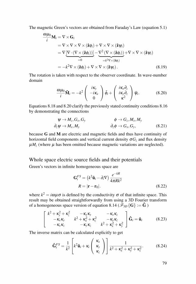
The magnetic Green’s vectors are obtained from Faraday’s Law (equation 5.1)ωµ0

iMi = ∇×Gi

= ∇×∇×∇× (zφi)+∇×∇× (zψi)

= ∇ [∇ · (∇× (zφi))]︸ ︷︷ ︸=0

−∇2 (∇× (zφi))︸ ︷︷ ︸=k2∇×(zφi)

+∇×∇× (zψi)

=−k2∇× (zφi)+∇×∇× (zψi) . (8.19)

The rotation is taken with respect to the observer coordinate. In wave-numberdomain

ωµ0

iMi =−k2

iκy−iκx

0

φi +

iκx∂ziκy∂zκ2

ψi. (8.20)

Equations 8.18 and 8.20 clarify the previously stated continuity conditions 8.16by demonstrating the connections

ψ →Mz,Gx,Gy φ → Gz,Mx,My

∂zψ →Mx,My ∂zφ → Gx,Gy, (8.21)

because G and M are electric and magnetic fields and thus have continuity ofhorizontal field components and vertical current density σGz and flux densityµMz (where µ has been omitted because magnetic variations are neglected).

Whole space electric source fields and their potentialsGreen’s vectors in infinite homogeneous space are

GFSi =

(k2ui−∂i∇

) e−kR

4πRk2

R = |r− r0|. (8.22)

where k2 = iωµσ is defined by the conductivity σ of that infinite space. Thisresult may be obtained straightforwardly from using a 3D Fourier transformof a homogeneous space version of equation 8.14 (F3D G := G ) k2 +κ2

y +κ2z −κxκy −κxκz

−κxκy k2 +κ2x +κ2

z −κyκz−κxκz −κyκz k2 +κ2

x +κ2y

Gi = ui (8.23)

The inverse matrix can be calculated explicitly to get

GFSi =

1k2

k2ui +κi

κxκyκz

1k2 +κ2

x +κ2y +κ2

z. (8.24)

79

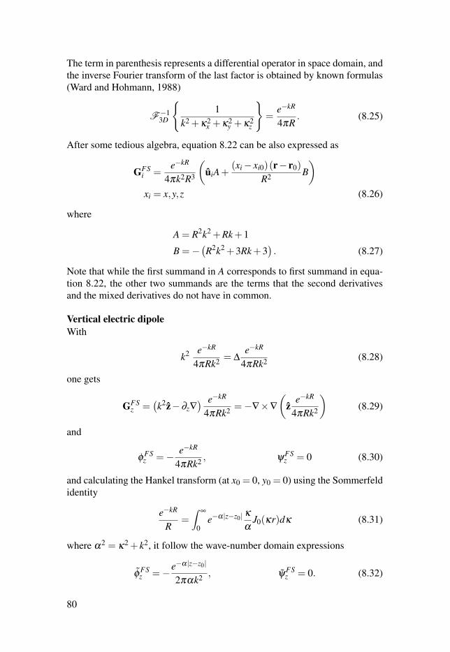
The term in parenthesis represents a differential operator in space domain, andthe inverse Fourier transform of the last factor is obtained by known formulas(Ward and Hohmann, 1988)

F−13D

1

k2 +κ2x +κ2

y +κ2z

=

e−kR

4πR. (8.25)

After some tedious algebra, equation 8.22 can be also expressed as

GFSi =

e−kR

4πk2R3

(uiA+

(xi− xi0)(r− r0)

R2 B)

xi = x,y,z (8.26)

where

A = R2k2 +Rk+1

B =−(R2k2 +3Rk+3

). (8.27)

Note that while the first summand in A corresponds to first summand in equa-tion 8.22, the other two summands are the terms that the second derivativesand the mixed derivatives do not have in common.

Vertical electric dipoleWith

k2 e−kR

4πRk2 = ∆e−kR

4πRk2 (8.28)

one gets

GFSz =

(k2z−∂z∇

) e−kR

4πRk2 =−∇×∇

(z

e−kR

4πRk2

)(8.29)

and

φFSz =− e−kR

4πRk2 , ψFSz = 0 (8.30)

and calculating the Hankel transform (at x0 = 0, y0 = 0) using the Sommerfeldidentity

e−kR

R=∫

∞

0e−α|z−z0| κ

αJ0(κr)dκ (8.31)

where α2 = κ2 + k2, it follow the wave-number domain expressions

φFSz =−e−α|z−z0|

2παk2 , ψFSz = 0. (8.32)

80

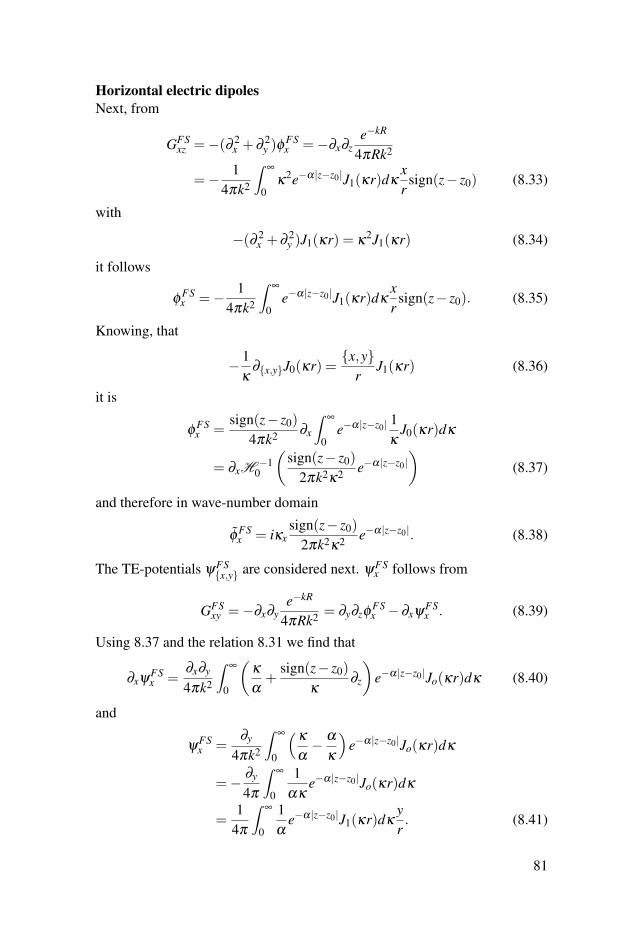
Horizontal electric dipolesNext, from

GFSxz =−(∂ 2

x +∂2y )φ

FSx =−∂x∂z

e−kR

4πRk2

=− 14πk2

∫∞

0κ

2e−α|z−z0|J1(κr)dκxr

sign(z− z0) (8.33)

with

−(∂ 2x +∂

2y )J1(κr) = κ

2J1(κr) (8.34)

it follows

φFSx =− 1

4πk2

∫∞

0e−α|z−z0|J1(κr)dκ

xr

sign(z− z0). (8.35)

Knowing, that

− 1κ

∂x,yJ0(κr) =x,y

rJ1(κr) (8.36)

it is

φFSx =

sign(z− z0)

4πk2 ∂x

∫∞

0e−α|z−z0| 1

κJ0(κr)dκ

= ∂xH−1

0

(sign(z− z0)

2πk2κ2 e−α|z−z0|)

(8.37)

and therefore in wave-number domain

φFSx = iκx

sign(z− z0)

2πk2κ2 e−α|z−z0|. (8.38)

The TE-potentials ψFSx,y are considered next. ψFS

x follows from

GFSxy =−∂x∂y

e−kR

4πRk2 = ∂y∂zφFSx −∂xψ

FSx . (8.39)

Using 8.37 and the relation 8.31 we find that

∂xψFSx =

∂x∂y

4πk2

∫∞

0

(κ

α+

sign(z− z0)

κ∂z

)e−α|z−z0|Jo(κr)dκ (8.40)

and

ψFSx =

∂y

4πk2

∫∞

0

(κ

α− α

κ

)e−α|z−z0|Jo(κr)dκ

=−∂y

4π

∫∞

0

1ακ

e−α|z−z0|Jo(κr)dκ

=1

4π

∫∞

0

1α

e−α|z−z0|J1(κr)dκyr. (8.41)

81

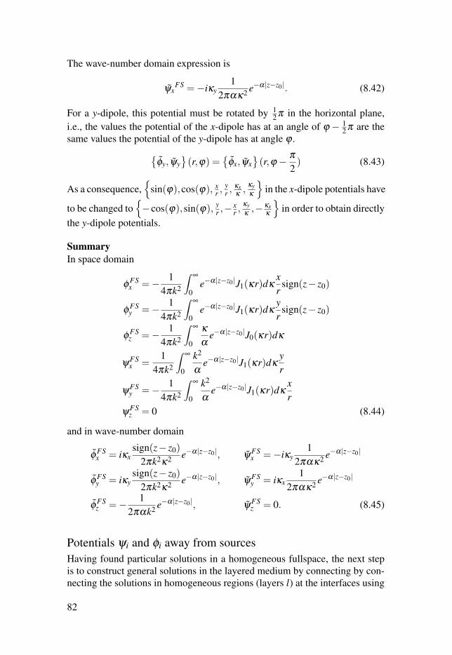
The wave-number domain expression is

ψxFS =−iκy

12πακ2 e−α|z−z0|. (8.42)

For a y-dipole, this potential must be rotated by 12 π in the horizontal plane,

i.e., the values the potential of the x-dipole has at an angle of ϕ − 12 π are the

same values the potential of the y-dipole has at angle ϕ .φy, ψy

(r,ϕ) =

φx, ψx

(r,ϕ− π

2) (8.43)

As a consequence,

sin(ϕ),cos(ϕ), xr ,

yr ,

κxκ,

κyκ

in the x-dipole potentials have

to be changed to−cos(ϕ),sin(ϕ), y

r ,−xr ,

κyκ,−κx

κ

in order to obtain directly

the y-dipole potentials.

SummaryIn space domain

φFSx =− 1

4πk2

∫∞

0e−α|z−z0|J1(κr)dκ

xr

sign(z− z0)

φFSy =− 1

4πk2

∫∞

0e−α|z−z0|J1(κr)dκ

yr

sign(z− z0)

φFSz =− 1

4πk2

∫∞

0

κ

αe−α|z−z0|J0(κr)dκ

ψFSx =

14πk2

∫∞

0

k2

αe−α|z−z0|J1(κr)dκ

yr

ψFSy =− 1

4πk2

∫∞

0

k2

αe−α|z−z0|J1(κr)dκ

xr

ψFSz = 0 (8.44)

and in wave-number domain

φFSx = iκx

sign(z− z0)

2πk2κ2 e−α|z−z0|, ψFSx =−iκy

12πακ2 e−α|z−z0|

φFSy = iκy

sign(z− z0)

2πk2κ2 e−α|z−z0|, ψFSy = iκx

12πακ2 e−α|z−z0|

φFSz =− 1

2παk2 e−α|z−z0|, ψFSz = 0. (8.45)

Potentials ψi and φi away from sourcesHaving found particular solutions in a homogeneous fullspace, the next stepis to construct general solutions in the layered medium by connecting by con-necting the solutions in homogeneous regions (layers l) at the interfaces using

82

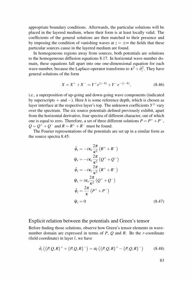
appropriate boundary conditions. Afterwards, the particular solutions will beplaced in the layered medium, where their form is at least locally valid. Thecoefficients of the general solutions are then matched to their presence andby imposing the condition of vanishing waves at z = ±∞ the fields that theseparticular sources cause in the layered medium are found.

In homogeneous regions away from sources, both potentials are solutionsto the homogeneous diffusion equations 8.17. In horizontal wave-number do-main, these equations fall apart into one one-dimensional equation for eachwave-number, because the Laplace-operator transforms to κ2+∂ 2

z . They havegeneral solutions of the form

X = X++X− = Y+e(z−h)+Y−e−(z−h), (8.46)

i.e., a superposition of up-going and down-going wave components (indicatedby superscripts + and −). Here h is some reference depth, which is chosen aslayer interface at the respective layer’s top. The unknown coefficients Y± varyover the spectrum. The six source potentials defined previously exhibit, apartfrom the horizontal derivative, four spectra of different character, out of whichone is equal to zero. Therefore, a set of three different solutions P = P++P−,Q = Q++Q− and R = R++R− must be found.

The Fourier representations of the potentials are set up in a similar form asthe source spectra 8.45:

φx =−iκx2π

κ2

(R++R−

)ψx =−iκy

2π

κ2

(Q++Q−

)φy =−iκy

2π

κ2

(R++R−

)ψy = iκx

2π

κ2

(Q++Q−

)φz =

2π

κ

(P++P−

)ψz = 0 (8.47)

Explicit relation between the potentials and Green’s tensorBefore finding those solutions, observe how Green’s tensor elements in wave-number domain are expressed in terms of P, Q and R. Be the r-coordinate(field coordinate) in layer l, we have

∂z(P,Q,R++P,Q,R−

)= αl

(P,Q,R+−P,Q,R−

)(8.48)

83

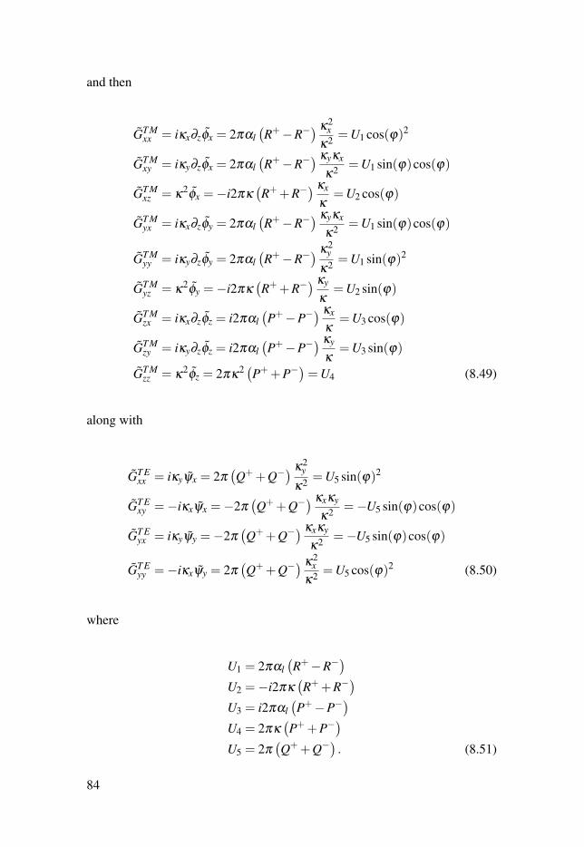
and then

GT Mxx = iκx∂zφx = 2παl

(R+−R−

) κ2x

κ2 =U1 cos(ϕ)2

GT Mxy = iκy∂zφx = 2παl

(R+−R−

) κyκx

κ2 =U1 sin(ϕ)cos(ϕ)

GT Mxz = κ

2φx =−i2πκ

(R++R−

) κx

κ=U2 cos(ϕ)

GT Myx = iκx∂zφy = 2παl

(R+−R−

) κyκx

κ2 =U1 sin(ϕ)cos(ϕ)

GT Myy = iκy∂zφy = 2παl

(R+−R−

) κ2y

κ2 =U1 sin(ϕ)2

GT Myz = κ

2φy =−i2πκ

(R++R−

) κy

κ=U2 sin(ϕ)

GT Mzx = iκx∂zφz = i2παl

(P+−P−

) κx

κ=U3 cos(ϕ)

GT Mzy = iκy∂zφz = i2παl

(P+−P−

) κy

κ=U3 sin(ϕ)

GT Mzz = κ

2φz = 2πκ

2 (P++P−)=U4 (8.49)

along with

GT Exx = iκyψx = 2π

(Q++Q−

) κ2y

κ2 =U5 sin(ϕ)2

GT Exy =−iκxψx =−2π

(Q++Q−

) κxκy

κ2 =−U5 sin(ϕ)cos(ϕ)

GT Eyx = iκyψy =−2π

(Q++Q−

) κxκy

κ2 =−U5 sin(ϕ)cos(ϕ)

GT Eyy =−iκxψy = 2π

(Q++Q−

) κ2x

κ2 =U5 cos(ϕ)2 (8.50)

where

U1 = 2παl(R+−R−

)U2 =−i2πκ

(R++R−

)U3 = i2παl

(P+−P−

)U4 = 2πκ

(P++P−

)U5 = 2π

(Q++Q−

). (8.51)

84

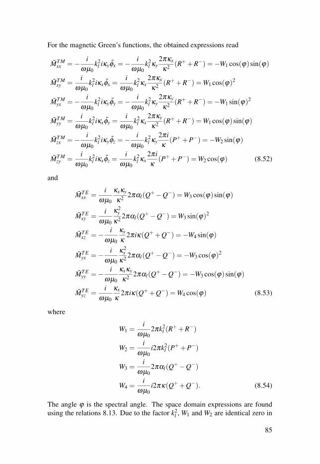
For the magnetic Green’s functions, the obtained expressions read

MT Mxx =− i

ωµ0k2

l iκyφx =−i

ωµ0k2

l κy2πκx

κ2 (R++R−) =−W1 cos(ϕ)sin(ϕ)

MT Mxy =

iωµ0

k2l iκxφx =

iωµ0

k2l κx

2πκx

κ2 (R++R−) =W1 cos(ϕ)2

MT Myx =− i

ωµ0k2

l iκyφy =−i

ωµ0k2

l κy2πκy

κ2 (R++R−) =−W1 sin(ϕ)2

MT Myy =

iωµ0

k2l iκxφy =

iωµ0

k2l κx

2πκy

κ2 (R++R−) =W1 cos(ϕ)sin(ϕ)

MT Mzx =− i

ωµ0k2

l iκyφz =−i

ωµ0k2

l κy2πiκ

(P++P−) =−W2 sin(ϕ)

MT Mzy =

iωµ0

k2l iκxφz =

iωµ0

k2l κx

2πiκ

(P++P−) =W2 cos(ϕ) (8.52)

and

MT Exx =

iωµ0

κxκy

κ2 2παl(Q+−Q−) =W3 cos(ϕ)sin(ϕ)

MT Exy =

iωµ0

κ2y

κ2 2παl(Q+−Q−) =W3 sin(ϕ)2

MT Exz =− i

ωµ0

κy

κ2πiκ(Q++Q−) =−W4 sin(ϕ)

MT Eyx =− i

ωµ0

κ2x

κ2 2παl(Q+−Q−) =−W3 cos(ϕ)2

MT Eyy =− i

ωµ0

κxκy

κ2 2παl(Q+−Q−) =−W3 cos(ϕ)sin(ϕ)

MT Eyz =

iωµ0

κx

κ2πiκ(Q++Q−) =W4 cos(ϕ) (8.53)

where

W1 =i

ωµ02πk2

l (R++R−)

W2 =i

ωµ0i2πk2

l (P++P−)

W3 =i

ωµ02παl(Q+−Q−)

W4 =i

ωµ0i2πκ(Q++Q−). (8.54)

The angle ϕ is the spectral angle. The space domain expressions are foundusing the relations 8.13. Due to the factor k2

l , W1 and W2 are identical zero in

85

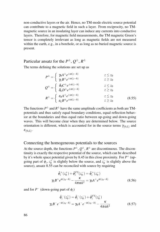
non-conductive layers or the air. Hence, no TM-mode electric source potentialcan contribute to a magnetic field in such a layer. From reciprocity, no TM-magnetic source in an insulating layer can induce any currents into conductivelayers. Therefore, for magnetic field measurements, the TM magnetic Green’stensor is completely irrelevant as long as magnetic fields are not measuredwithin the earth, e.g., in a borehole, or as long as no buried magnetic source ispresent.

Particular ansatz for the P±, Q±, R±

The terms defining the solutions are set up as

P± =

γ0A±e±α(z−h)

γLB±e±α(z−h)z≤ z0z≥ z0

Q± =

δ0C±e±α(z−h)

δLD±e±α(z−h)z≤ z0z≥ z0

R± =

ε0A±e±α(z−h)

εLB±e±α(z−h)z≤ z0z≥ z0

(8.55)

The functions P± and R± have the same amplitude coefficients as both are TM-potentials and thus satisfy equal boundary conditions, equal reflection behav-ior at the boundaries and thus equal ratio between up-going and down-goingwaves. This will become clear when they are determined below. The sourceorientation is different, which is accounted for in the source terms γ0,L andε0,L.

Connecting the homogeneous potentials to the sourcesAt the source depth, the functions P±, Q±, R± are discontinuous. The discon-tinuity is exactly the respective potential of the source, which can be describedby it’s whole space potential given by 8.45 in this close proximity. For P+ (up-going part of φz, z+0 is slightly below the source, and z−0 is slightly above thesource), ansatz 8.55 can be reconciled with source by requiring

φ+z (z+0 )+ φ

FSz (z−0 ) = φ

+z (z−0 )

γLB+eα(z0−h)− κ

4παk2 = γ0A+eα(z0−h) (8.56)

and for P− (down-going part of φz)

φ−z (z+0 ) = φ

−z (z−0 )+ φ

FSz (z+0 )

γLB−e−α(z0−h) = γ0A−e−α(z0−h)− κ

4παk2 (8.57)

86

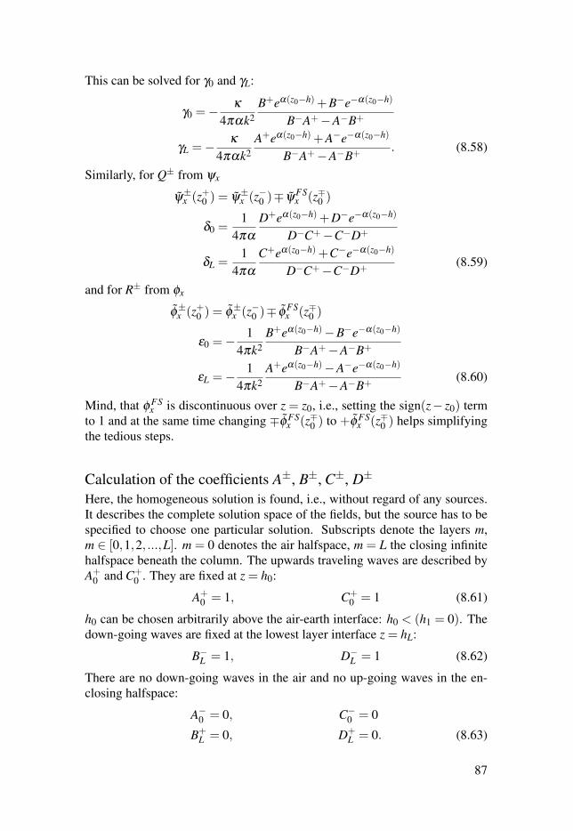
This can be solved for γ0 and γL:

γ0 =−κ

4παk2B+eα(z0−h)+B−e−α(z0−h)

B−A+−A−B+

γL =− κ

4παk2A+eα(z0−h)+A−e−α(z0−h)

B−A+−A−B+. (8.58)

Similarly, for Q± from ψx

ψ±x (z+0 ) = ψ

±x (z−0 )∓ ψ

FSx (z∓0 )

δ0 =1

4πα

D+eα(z0−h)+D−e−α(z0−h)

D−C+−C−D+

δL =1

4πα

C+eα(z0−h)+C−e−α(z0−h)

D−C+−C−D+(8.59)

and for R± from φx

φ±x (z+0 ) = φ

±x (z−0 )∓ φ

FSx (z∓0 )

ε0 =−1

4πk2B+eα(z0−h)−B−e−α(z0−h)

B−A+−A−B+

εL =− 14πk2

A+eα(z0−h)−A−e−α(z0−h)

B−A+−A−B+(8.60)

Mind, that φ FSx is discontinuous over z = z0, i.e., setting the sign(z− z0) term

to 1 and at the same time changing ∓φ FSx (z∓0 ) to +φ FS

x (z∓0 ) helps simplifyingthe tedious steps.

Calculation of the coefficients A±, B±, C±, D±

Here, the homogeneous solution is found, i.e., without regard of any sources.It describes the complete solution space of the fields, but the source has to bespecified to choose one particular solution. Subscripts denote the layers m,m ∈ [0,1,2, ...,L]. m = 0 denotes the air halfspace, m = L the closing infinitehalfspace beneath the column. The upwards traveling waves are described byA+

0 and C+0 . They are fixed at z = h0:

A+0 = 1, C+

0 = 1 (8.61)

h0 can be chosen arbitrarily above the air-earth interface: h0 < (h1 = 0). Thedown-going waves are fixed at the lowest layer interface z = hL:

B−L = 1, D−L = 1 (8.62)

There are no down-going waves in the air and no up-going waves in the en-closing halfspace:

A−0 = 0, C−0 = 0

B+L = 0, D+

L = 0. (8.63)

87

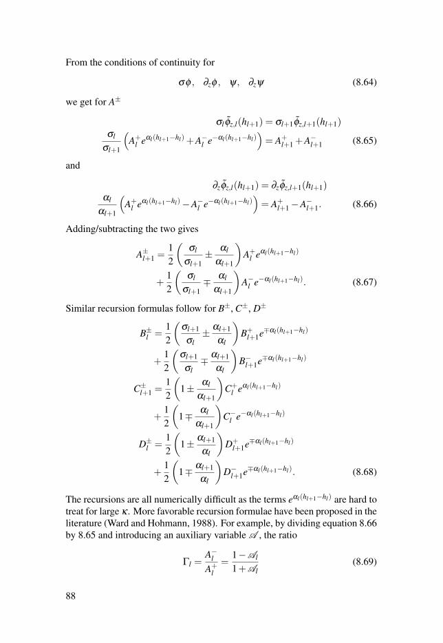
From the conditions of continuity for

σφ , ∂zφ , ψ, ∂zψ (8.64)

we get for A±

σl φz,l(hl+1) = σl+1φz,l+1(hl+1)σl

σl+1

(A+

l eαl(hl+1−hl)+A−l e−αl(hl+1−hl))= A+

l+1 +A−l+1 (8.65)

and

∂zφz,l(hl+1) = ∂zφz,l+1(hl+1)αl

αl+1

(A+

l eαl(hl+1−hl)−A−l e−αl(hl+1−hl))= A+

l+1−A−l+1. (8.66)

Adding/subtracting the two gives

A±l+1 =12

(σl

σl+1± αl

αl+1

)A+

l eαl(hl+1−hl)

+12

(σl

σl+1∓ αl

αl+1

)A−l e−αl(hl+1−hl). (8.67)

Similar recursion formulas follow for B±, C±, D±

B±l =12

(σl+1

σl± αl+1

αl

)B+

l+1e∓αl(hl+1−hl)

+12

(σl+1

σl∓ αl+1

αl

)B−l+1e∓αl(hl+1−hl)

C±l+1 =12

(1± αl

αl+1

)C+

l eαl(hl+1−hl)

+12

(1∓ αl

αl+1

)C−l e−αl(hl+1−hl)

D±l =12

(1± αl+1

αl

)D+

l+1e∓αl(hl+1−hl)

+12

(1∓ αl+1

αl

)D−l+1e∓αl(hl+1−hl). (8.68)

The recursions are all numerically difficult as the terms eαl(hl+1−hl) are hard totreat for large κ . More favorable recursion formulae have been proposed in theliterature (Ward and Hohmann, 1988). For example, by dividing equation 8.66by 8.65 and introducing an auxiliary variable A , the ratio

Γl =A−lA+

l=

1−Al

1+Al(8.69)

88

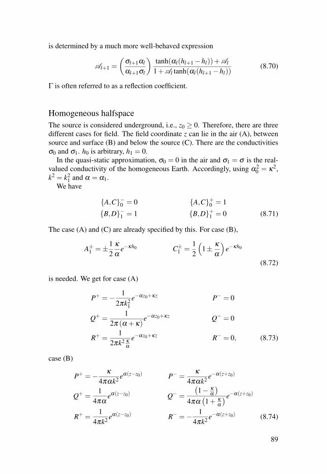
is determined by a much more well-behaved expression

Al+1 =

(σl+1αl

αl+1σl

)tanh(αl(hl+1−hl))+Al

1+Al tanh(αl(hl+1−hl))(8.70)

Γ is often referred to as a reflection coefficient.

Homogeneous halfspaceThe source is considered underground, i.e., z0 ≥ 0. Therefore, there are threedifferent cases for field. The field coordinate z can lie in the air (A), betweensource and surface (B) and below the source (C). There are the conductivitiesσ0 and σ1. h0 is arbitrary, h1 = 0.

In the quasi-static approximation, σ0 = 0 in the air and σ1 = σ is the real-valued conductivity of the homogeneous Earth. Accordingly, using α2

0 = κ2,k2 = k2

1 and α = α1.We have

A,C−0 = 0 A,C+0 = 1

B,D−1 = 1 B,D+1 = 0 (8.71)

The case (A) and (C) are already specified by this. For case (B),

A±1 =±12

κ

αe−κh0 C±1 =

12

(1± κ

α

)e−κh0

(8.72)

is needed. We get for case (A)

P+ =− 12πk2

1e−αz0+κz P− = 0

Q+ =1

2π (α +κ)e−αz0+κz Q− = 0

R+ =1

2πk2 κ

α

e−αz0+κz R− = 0, (8.73)

case (B)

P+ =− κ

4παk2 eα(z−z0) P− =κ

4παk2 e−α(z+z0)

Q+ =1

4παeα(z−z0) Q− =

(1− κ

α

)4πα

(1+ κ

α

)e−α(z+z0)

R+ =1

4πk2 eα(z−z0) R− =− 14πk2 e−α(z+z0) (8.74)

89

and case (C)

P+ = 0 P− =− κ

4παk2

(e−α(z−z0)− e−α(z+z0)

)Q+ = 0 Q− =

14πα

(e−α(z−z0)+

1− κ

α

1+ κ

α

e−α(z+z0)

)R+ = 0 R− =− 1

4πk2

(e−α(z−z0)+ e−α(z+z0)

). (8.75)

These expressions can be substituted backwards into the general expressionsof Green’s tensor (see above) to obtain their wave-number domain forms. Thespace domain formulation is then obtained using inverse Fourier or Hankeltransforms.

Analytic solutionIn the quasi-analytic case, the integration of the Hankel integrals can be car-ried out explicitly for the cases (B) and (C). The closed expressions are givenby Weidelt (1975) or Raiche (1975). They can be derived using the knownintegrals∫

∞

0

κ

αe−αzJ0(κr)dκ =

e−kR

R(8.76)∫

∞

0

1α

e−αzJ0(κr)dκ = I0

[12

k (R− z)]

K0

[12

k (R+ z)]. (8.77)

Equation 8.76 is known as the Sommerfeld integral, equation 8.77 can forexample be found in Gradshteyn and Ryzhik (2000), 6.637.1. Defining

R2± = (x− x0)

2 +(y− y0)2 +(z± z0)

2

g± =e−kR±

4πR±

γ = ∂z

I0

[12

k (R+− z− z0)

]K0

[12

k (R++ z+ z0)

]/(2π)

= ∂z0

I0

[12

k (R+− z− z0)

]K0

[12

k (R++ z+ z0)

]/(2π) (8.78)

the tensor elements for z,z0 > 0 read

k2Gxx,yy =[k2−∂

2x,y

](g−−g+− γ)+∂

2z (2g++ γ)

k2Gxy,yx =−∂x∂y (g−−g+− γ)

k2Gxz,yz =−∂x,y∂z (g−+g+)

k2Gzx,zy =−∂x,y∂z (g−−g+)

k2Gzz =[k2−∂

2z](g−−g+) (8.79)

90

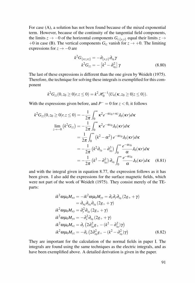
For case (A), a solution has not been found because of the mixed exponentialterm. However, because of the continuity of the tangential field components,the limits z→−0 of the horizontal components Gi,x,y equal their limits z→+0 in case (B). The vertical components Giz vanish for z→+0. The limitingexpressions for z→−0 are

k2Gxz,yz =−∂x,y∂z0γ

k2Gzz =−[k2−∂

2z0

]γ (8.80)

The last of these expressions is different than the one given by Weidelt (1975).Therefore, the technique for solving these integrals is exemplified for this com-ponent

k2Gzz(0,z0 ≥ 0|r,z≤ 0) = k2H −10 (U4(κ,z0 ≥ 0|z≤ 0)).

With the expressions given before, and P− = 0 for z < 0, it follows

k2Gzz(0,z0 ≥ 0|r,z≤ 0) =− 12π

∫∞

0κ

2e−αz0+κzJ0(κr)dκ

limz→−0

(k2Gzz

)=− 1

2π

∫∞

0κ

2e−αz0J0(κr)dκ

=1

2π

∫∞

0

(k2−α

2)e−αz0J0(κr)dκ

=− 12π

(k2

∂z0−∂3z0

)∫ ∞

0

e−αz0

αJ0(κr)dκ

=− 12π

(k2−∂

2z0

)∂z0

∫∞

0

e−αz0

αJ0(κr)dκ (8.81)

and with the integral given in equation 8.77, the expression follows as it hasbeen given. I also add the expressions for the surface magnetic fields, whichwere not part of the work of Weidelt (1975). They consist merely of the TE-parts:

ik2ωµ0Mxx =−ik2

ωµ0Myy = ∂x∂y∂z0 (2g++ γ)

= ∂x0∂y0∂z0 (2g++ γ)

ik2ωµ0Mxy = ∂

2y ∂z0 (2g++ γ)

ik2ωµ0Myx =−∂

2x ∂z0 (2g++ γ)

ik2ωµ0Mxz = ∂y

(2∂

2z0

g+− (k2−∂2z0)γ)

ik2ωµ0Myz =−∂x

(2∂

2z0

g+− (k2−∂2z0)γ)

(8.82)

They are important for the calculation of the normal fields in paper I. Theintegrals are found using the same techniques as the electric integrals, and ashave been exemplified above. A detailed derivation is given in the paper.

91

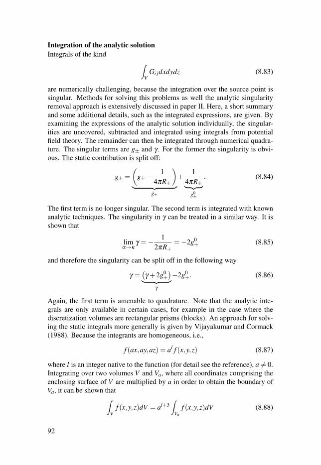
Integration of the analytic solutionIntegrals of the kind ∫

VGi jdxdydz (8.83)

are numerically challenging, because the integration over the source point issingular. Methods for solving this problems as well the analytic singularityremoval approach is extensively discussed in paper II. Here, a short summaryand some additional details, such as the integrated expressions, are given. Byexamining the expressions of the analytic solution individually, the singular-ities are uncovered, subtracted and integrated using integrals from potentialfield theory. The remainder can then be integrated through numerical quadra-ture. The singular terms are g± and γ . For the former the singularity is obvi-ous. The static contribution is split off:

g± =

(g±−

14πR±

)︸ ︷︷ ︸

g±

+1

4πR±︸ ︷︷ ︸g0±

. (8.84)

The first term is no longer singular. The second term is integrated with knownanalytic techniques. The singularity in γ can be treated in a similar way. It isshown that

limα→κ

γ =− 12πR+

=−2g0+ (8.85)

and therefore the singularity can be split off in the following way

γ =(γ +2g0

+

)︸ ︷︷ ︸γ

−2g0+. (8.86)

Again, the first term is amenable to quadrature. Note that the analytic inte-grals are only available in certain cases, for example in the case where thediscretization volumes are rectangular prisms (blocks). An approach for solv-ing the static integrals more generally is given by Vijayakumar and Cormack(1988). Because the integrants are homogeneous, i.e.,

f (ax,ay,az) = al f (x,y,z) (8.87)

where l is an integer native to the function (for detail see the reference), a 6= 0.Integrating over two volumes V and Va, where all coordinates comprising theenclosing surface of V are multiplied by a in order to obtain the boundary ofVa, it can be shown that∫

Vf (x,y,z)dV = al+3

∫Va

f (x,y,z)dV (8.88)

92

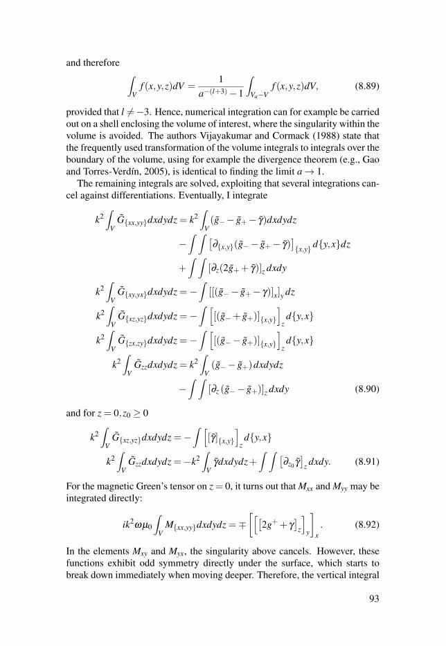
and therefore ∫V

f (x,y,z)dV =1

a−(l+3)−1

∫Va−V

f (x,y,z)dV, (8.89)

provided that l 6=−3. Hence, numerical integration can for example be carriedout on a shell enclosing the volume of interest, where the singularity within thevolume is avoided. The authors Vijayakumar and Cormack (1988) state thatthe frequently used transformation of the volume integrals to integrals over theboundary of the volume, using for example the divergence theorem (e.g., Gaoand Torres-Verdín, 2005), is identical to finding the limit a→ 1.

The remaining integrals are solved, exploiting that several integrations can-cel against differentiations. Eventually, I integrate

k2∫

VGxx,yydxdydz = k2

∫V(g−− g+− γ)dxdydz

−∫ ∫ [

∂x,y(g−− g+− γ)]x,y dy,xdz

+∫ ∫

[∂z(2g++ γ)]z dxdy

k2∫

VGxy,yxdxdydz =−

∫[[(g−− g+− γ)]x]y dz

k2∫

VGxz,yzdxdydz =−

∫ [[(g−+ g+)]x,y

]zdy,x

k2∫

VGzx,zydxdydz =−

∫ [[(g−− g+)]x,y

]zdy,x

k2∫

VGzzdxdydz = k2

∫V(g−− g+)dxdydz

−∫ ∫

[∂z (g−− g+)]z dxdy (8.90)

and for z = 0,z0 ≥ 0

k2∫

VGxz,yzdxdydz =−

∫ [[γ]x,y

]zdy,x

k2∫

VGzzdxdydz =−k2

∫V

γdxdydz+∫ ∫ [

∂z0 γ]

z dxdy. (8.91)

For the magnetic Green’s tensor on z = 0, it turns out that Mxx and Myy may beintegrated directly:

ik2ωµ0

∫V

Mxx,yydxdydz =∓[[[

2g++ γ]

z

]y

]x. (8.92)

In the elements Mxy and Myx, the singularity above cancels. However, thesefunctions exhibit odd symmetry directly under the surface, which starts tobreak down immediately when moving deeper. Therefore, the vertical integral

93

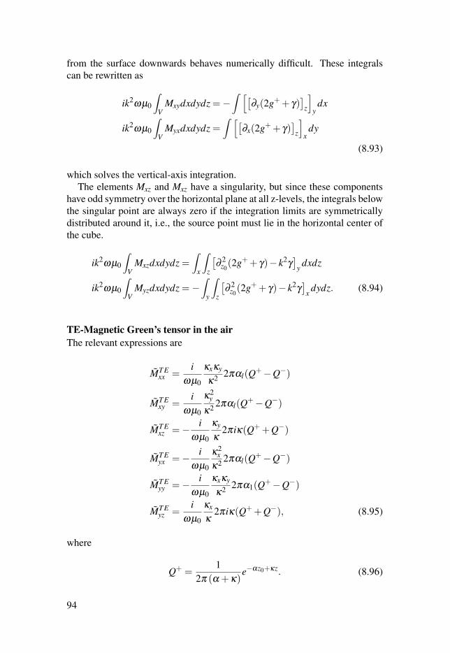
from the surface downwards behaves numerically difficult. These integralscan be rewritten as

ik2ωµ0

∫V

Mxydxdydz =−∫ [[

∂y(2g++ γ)]

z

]ydx

ik2ωµ0

∫V

Myxdxdydz =∫ [[

∂x(2g++ γ)]

z

]xdy

(8.93)

which solves the vertical-axis integration.The elements Mxz and Mxz have a singularity, but since these components

have odd symmetry over the horizontal plane at all z-levels, the integrals belowthe singular point are always zero if the integration limits are symmetricallydistributed around it, i.e., the source point must lie in the horizontal center ofthe cube.

ik2ωµ0

∫V

Mxzdxdydz =∫

x

∫z

[∂

2z0(2g++ γ)− k2

γ]

y dxdz

ik2ωµ0

∫V

Myzdxdydz =−∫

y

∫z

[∂

2z0(2g++ γ)− k2

γ]

x dydz. (8.94)

TE-Magnetic Green’s tensor in the airThe relevant expressions are

MT Exx =

iωµ0

κxκy

κ2 2παl(Q+−Q−)

MT Exy =

iωµ0

κ2y

κ2 2παl(Q+−Q−)

MT Exz =− i

ωµ0

κy

κ2πiκ(Q++Q−)

MT Eyx =− i

ωµ0

κ2x

κ2 2παl(Q+−Q−)

MT Eyy =− i

ωµ0

κxκy

κ2 2πα1(Q+−Q−)

MT Eyz =

iωµ0

κx

κ2πiκ(Q++Q−), (8.95)

where

Q+ =1

2π (α +κ)e−αz0+κz. (8.96)

94

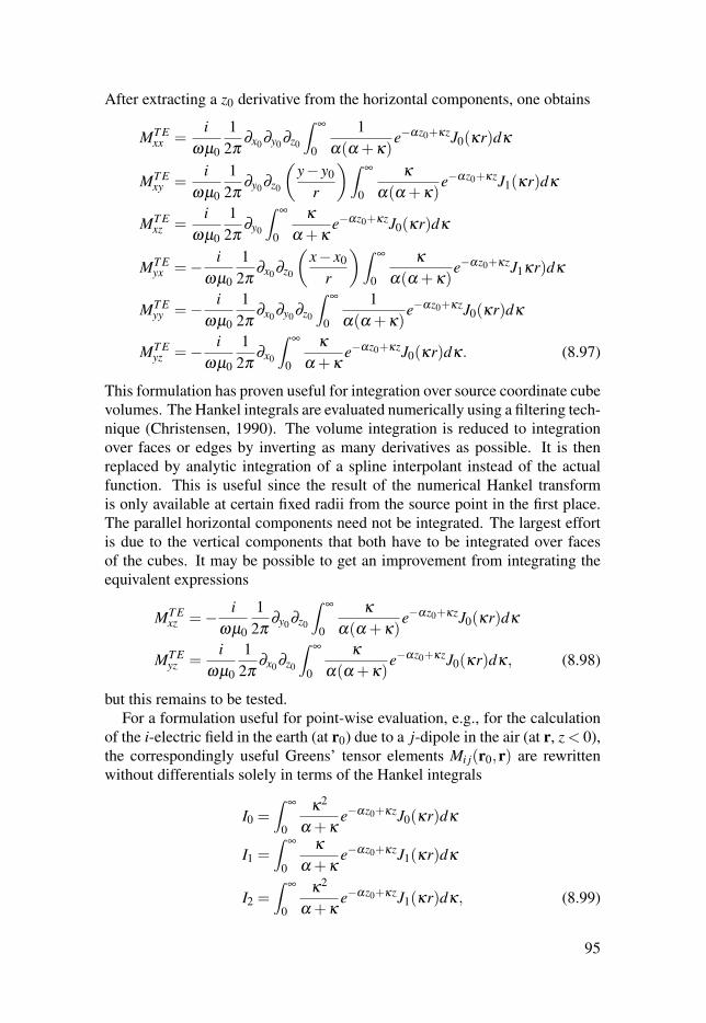
After extracting a z0 derivative from the horizontal components, one obtains

MT Exx =

iωµ0

12π

∂x0∂y0∂z0

∫∞

0

1α(α +κ)

e−αz0+κzJ0(κr)dκ

MT Exy =

iωµ0

12π

∂y0∂z0

(y− y0

r

)∫∞

0

κ

α(α +κ)e−αz0+κzJ1(κr)dκ

MT Exz =

iωµ0

12π

∂y0

∫∞

0

κ

α +κe−αz0+κzJ0(κr)dκ

MT Eyx =− i

ωµ0

12π

∂x0∂z0

(x− x0

r

)∫∞

0

κ

α(α +κ)e−αz0+κzJ1κr)dκ

MT Eyy =− i

ωµ0

12π

∂x0∂y0∂z0

∫∞

0

1α(α +κ)

e−αz0+κzJ0(κr)dκ

MT Eyz =− i

ωµ0

12π

∂x0

∫∞

0

κ

α +κe−αz0+κzJ0(κr)dκ. (8.97)

This formulation has proven useful for integration over source coordinate cubevolumes. The Hankel integrals are evaluated numerically using a filtering tech-nique (Christensen, 1990). The volume integration is reduced to integrationover faces or edges by inverting as many derivatives as possible. It is thenreplaced by analytic integration of a spline interpolant instead of the actualfunction. This is useful since the result of the numerical Hankel transformis only available at certain fixed radii from the source point in the first place.The parallel horizontal components need not be integrated. The largest effortis due to the vertical components that both have to be integrated over facesof the cubes. It may be possible to get an improvement from integrating theequivalent expressions

MT Exz =− i

ωµ0

12π

∂y0∂z0

∫∞

0

κ

α(α +κ)e−αz0+κzJ0(κr)dκ

MT Eyz =

iωµ0

12π

∂x0∂z0

∫∞

0

κ

α(α +κ)e−αz0+κzJ0(κr)dκ, (8.98)

but this remains to be tested.For a formulation useful for point-wise evaluation, e.g., for the calculation

of the i-electric field in the earth (at r0) due to a j-dipole in the air (at r, z < 0),the correspondingly useful Greens’ tensor elements Mi j(r0,r) are rewrittenwithout differentials solely in terms of the Hankel integrals

I0 =∫

∞

0

κ2

α +κe−αz0+κzJ0(κr)dκ

I1 =∫

∞

0

κ

α +κe−αz0+κzJ1(κr)dκ

I2 =∫

∞

0

κ2

α +κe−αz0+κzJ1(κr)dκ, (8.99)

95

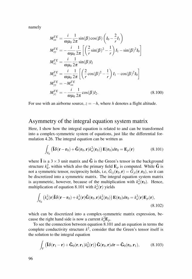
namely

MT Exx =

iωµ0

12π

sin(β )cos(β )(

I0−2r

I1

)MT E

xy =− iωµ0

12π

[(2r

sin(β )2− 1r

)I1− sin(β )2I0

]MT E

xz =i

ωµ0

12π

sin(β )I2

MT Eyx =

iωµ0

12π

[(2r

cos(β )2− 1r

)I1− cos(β )2I0

]MT E

yy =−MT Exx

MT Eyz =− i

ωµ0

12π

cos(β )I2. (8.100)

For use with an airborne source, z =−h, where h denotes a flight altitude.

Asymmetry of the integral equation system matrixHere, I show how the integral equation is related to and can be transformedinto a complex-symmetric system of equations, just like the differential for-mulation 4.26. The integral equation can be written as∫

V0

(Iδ (r− r0)+ G(r0,r)k2

a(r0))

E(r0)dr0 = Ep(r) (8.101)

where I is a 3× 3 unit matrix and G is the Green’s tensor in the backgroundstructure k2

b, within which also the primary field Ep is computed. While G isnot a symmetric tensor, reciprocity holds, i.e, Gi j(r0,r) = G ji(r,r0), so it canbe discretized into a symmetric matrix. The integral equation system matrixis asymmetric, however, because of the multiplication with k2

a(r0). Hence,multiplication of equation 8.101 with k2

a(r) yields∫V0

(k2

a(r)Iδ (r− r0)+ k2a(r)G(r0,r)k2

a(r0))

E(r0)dr0 = k2a(r)Ep(r),

(8.102)

which can be discretized into a complex-symmetric matrix expression, be-cause the right hand side is now a current k2

aEp.To see the connection between equation 8.101 and an equation in terms the

complete conductivity structure k2, consider that the Green’s tensor itself isthe solution to the integral equation∫

V

(Iδ (r1− r)+ G0(r,r1)k2

b(r))

G(r0,r)dr = G0(r0,r1), (8.103)

96

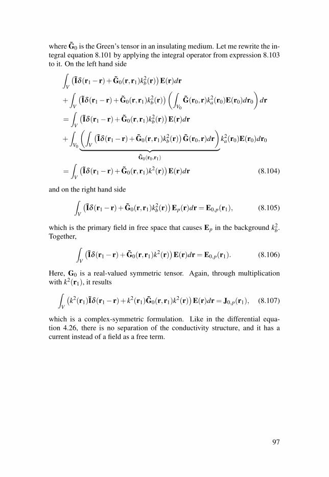
where G0 is the Green’s tensor in an insulating medium. Let me rewrite the in-tegral equation 8.101 by applying the integral operator from expression 8.103to it. On the left hand side∫

V

(Iδ (r1− r)+ G0(r,r1)k2

b(r))

E(r)dr

+∫

V

(Iδ (r1− r)+ G0(r,r1)k2

b(r))(∫

V0

G(r0,r)k2a(r0)E(r0)dr0

)dr

=∫

V

(Iδ (r1− r)+ G0(r,r1)k2

b(r))

E(r)dr

+∫

V0

(∫V

(Iδ (r1− r)+ G0(r,r1)k2

b(r))

G(r0,r)dr)

︸ ︷︷ ︸G0(r0,r1)

k2a(r0)E(r0)dr0

=∫

V

(Iδ (r1− r)+ G0(r,r1)k2(r)

)E(r)dr (8.104)

and on the right hand side∫V

(Iδ (r1− r)+ G0(r,r1)k2

b(r))

Ep(r)dr = E0,p(r1), (8.105)

which is the primary field in free space that causes Ep in the background k2b.

Together,∫V

(Iδ (r1− r)+ G0(r,r1)k2(r)

)E(r)dr = E0,p(r1). (8.106)

Here, G0 is a real-valued symmetric tensor. Again, through multiplicationwith k2(r1), it results∫

V

(k2(r1)Iδ (r1− r)+ k2(r1)G0(r,r1)k2(r)

)E(r)dr = J0,p(r1), (8.107)

which is a complex-symmetric formulation. Like in the differential equa-tion 4.26, there is no separation of the conductivity structure, and it has acurrent instead of a field as a free term.

97

Appendix B.A unified inversion and joint inversionframework

In this thesis, all inverse problems in this thesis are a part of the same inversionframework, which has been growing over the same time frame. Most code iswritten in MATLAB. Only certain bottlenecks where coded in C++.

Inversion schemes, in particular, joint inversion techniques continue to in-crease in complexity. Therefore, modular frameworks that allow fast assem-bly and reassambly of pre-existing parts is advantageous. Moorkamp et al.(2011) have presented an interesting framework previously, which has a dif-ferent structure than what has been used in this thesis. These authors organizethe joint inversion by modules, corresponding to geophysical method, and anadditional module for parameter transforms and regularization.

Variables and operatorsThe main idea underlying the implementation in this thesis is that inversion al-gorithms can be abstracted using variables and operators that transform vari-ables into one another. Variables represent the vectors in the algebraic equa-tions. Operators are functions (such as matrices) and their derivatives. Usingobject-oriented programming, this concept allows to quickly write general in-version algorithms on a high abstraction level. Together with the functionalityof operator and variable combination, as explained later on, complex inter-actions of forward operators, weightings, regularization operators, parametertransforms with data or model representations can be treated in a natural way.

Using object-oriented programming, variable and operator entities can beimplemented in terms of classes, i.e., templates for structures that contain dataand functions (denoted as methods). If such a structure is created in the com-puter memory from concrete values, it is called an instance of that class, ormore loosely an object. The class that an object has been created from isdenoted as its type. Another important concept are derived classes, which in-herit functionality from superclasses and add or adapt some of its aspects. Fora detailed explanation of object-oriented programming, see for example Eckel(2000).

Variables are implemented in the Variable-class or any derived subclass.Variable objects represent in this context either measurements (simulated or

98

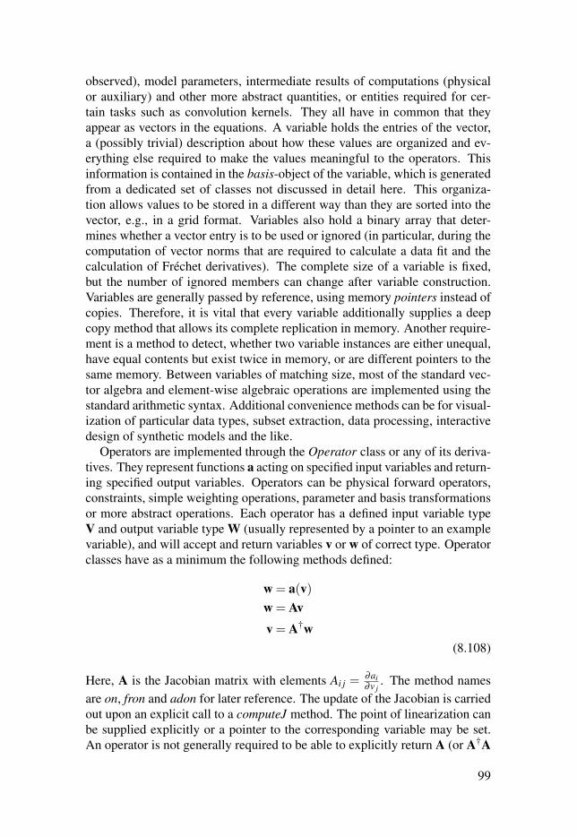
observed), model parameters, intermediate results of computations (physicalor auxiliary) and other more abstract quantities, or entities required for cer-tain tasks such as convolution kernels. They all have in common that theyappear as vectors in the equations. A variable holds the entries of the vector,a (possibly trivial) description about how these values are organized and ev-erything else required to make the values meaningful to the operators. Thisinformation is contained in the basis-object of the variable, which is generatedfrom a dedicated set of classes not discussed in detail here. This organiza-tion allows values to be stored in a different way than they are sorted into thevector, e.g., in a grid format. Variables also hold a binary array that deter-mines whether a vector entry is to be used or ignored (in particular, during thecomputation of vector norms that are required to calculate a data fit and thecalculation of Fréchet derivatives). The complete size of a variable is fixed,but the number of ignored members can change after variable construction.Variables are generally passed by reference, using memory pointers instead ofcopies. Therefore, it is vital that every variable additionally supplies a deepcopy method that allows its complete replication in memory. Another require-ment is a method to detect, whether two variable instances are either unequal,have equal contents but exist twice in memory, or are different pointers to thesame memory. Between variables of matching size, most of the standard vec-tor algebra and element-wise algebraic operations are implemented using thestandard arithmetic syntax. Additional convenience methods can be for visual-ization of particular data types, subset extraction, data processing, interactivedesign of synthetic models and the like.

Operators are implemented through the Operator class or any of its deriva-tives. They represent functions a acting on specified input variables and return-ing specified output variables. Operators can be physical forward operators,constraints, simple weighting operations, parameter and basis transformationsor more abstract operations. Each operator has a defined input variable typeV and output variable type W (usually represented by a pointer to an examplevariable), and will accept and return variables v or w of correct type. Operatorclasses have as a minimum the following methods defined:

w = a(v)w = Av

v = A†w(8.108)

Here, A is the Jacobian matrix with elements Ai j =∂ai∂v j

. The method namesare on, fron and adon for later reference. The update of the Jacobian is carriedout upon an explicit call to a computeJ method. The point of linearization canbe supplied explicitly or a pointer to the corresponding variable may be set.An operator is not generally required to be able to explicitly return A (or A†A

99

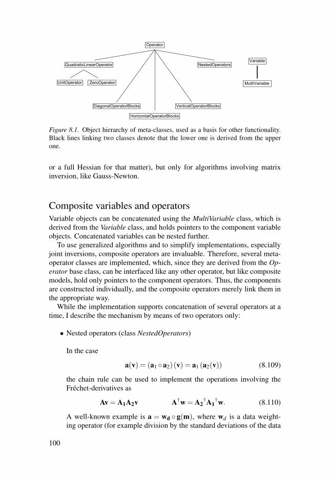
Operator

DiagonalOperatorBlocks

HorizontalOperatorBlocks

NestedOperatorsQuadraticLinearOperator

VerticalOperatorBlocks

UnitOperator ZeroOperator

Variable

MultiVariable

Figure 8.1. Object hierarchy of meta-classes, used as a basis for other functionality.Black lines linking two classes denote that the lower one is derived from the upperone.

or a full Hessian for that matter), but only for algorithms involving matrixinversion, like Gauss-Newton.

Composite variables and operatorsVariable objects can be concatenated using the MultiVariable class, which isderived from the Variable class, and holds pointers to the component variableobjects. Concatenated variables can be nested further.

To use generalized algorithms and to simplify implementations, especiallyjoint inversions, composite operators are invaluable. Therefore, several meta-operator classes are implemented, which, since they are derived from the Op-erator base class, can be interfaced like any other operator, but like compositemodels, hold only pointers to the component operators. Thus, the componentsare constructed individually, and the composite operators merely link them inthe appropriate way.

While the implementation supports concatenation of several operators at atime, I describe the mechanism by means of two operators only:

• Nested operators (class NestedOperators)

In the case

a(v) = (a1 a2)(v) = a1 (a2(v)) (8.109)

the chain rule can be used to implement the operations involving theFréchet-derivatives as

Av = A1A2v A†w = A2†A1

†w. (8.110)

A well-known example is a = wd g(m), where wd is a data weight-ing operator (for example division by the standard deviations of the data

100

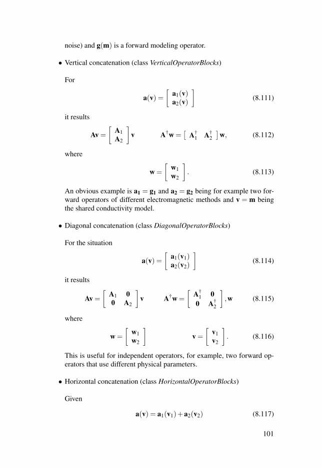
noise) and g(m) is a forward modeling operator.

• Vertical concatenation (class VerticalOperatorBlocks)

For

a(v) =[

a1(v)a2(v)

](8.111)

it results

Av =

[A1A2

]v A†w =

[A†

1 A†2

]w, (8.112)

where

w =

[w1w2

]. (8.113)

An obvious example is a1 = g1 and a2 = g2 being for example two for-ward operators of different electromagnetic methods and v = m beingthe shared conductivity model.

• Diagonal concatenation (class DiagonalOperatorBlocks)

For the situation

a(v) =[

a1(v1)a2(v2)

](8.114)

it results

Av =

[A1 00 A2

]v A†w =

[A†

1 00 A†

2

],w (8.115)

where

w =

[w1w2

]v =

[v1v2

]. (8.116)

This is useful for independent operators, for example, two forward op-erators that use different physical parameters.

• Horizontal concatenation (class HorizontalOperatorBlocks)

Given

a(v) = a1(v1)+a2(v2) (8.117)

101

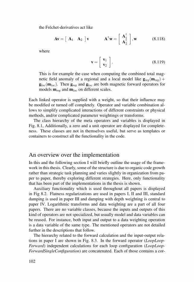
the Fréchet-derivatives act like

Av =[

A1 A2]

v A†w =

[A†

1A†

2

],w (8.118)

where

v =

[v1v2

]. (8.119)

This is for example the case when computing the combined total mag-netic field anomaly of a regional and a local model like greg(mreg) +gloc(mloc). Then greg and gloc are both magnetic forward operators formodels mreg and mloc on different scales.

Each linked operator is supplied with a weight, so that their influence maybe modified or turned off completely. Operator and variable combination al-lows to simplify complicated interactions of different constraints or physicalmethods, and/or complicated parameter weightings or transforms.

The class hierarchy of the meta operators and variables is displayed inFig. 8.1, Additionally, a zero and a unit operator are displayed for complete-ness. These classes are not in themselves useful, but serve as templates orcontainers to construct all the functionality in the code.

An overview over the implementationIn this and the following section I will briefly outline the usage of the frame-work in this thesis. Clearly, some of the structure is due to organic code growthrather than strategic task planning and varies slightly in organization from pa-per to paper, thereby exploring different strategies. Here, only functionalitythat has been part of the implementations in the thesis is shown.

Auxiliary functionality which is used throughout all papers is displayedin Fig 8.2. Flatness regularizations are used in papers I, II and III, standarddamping is used in paper III and damping with depth weighting is central topaper IV. Logarithmic transforms and data weighting are a part of all fourpapers. There are no variable classes, because the inputs and outputs of thiskind of operators are not specialized, but usually model and data variables canbe reused. For instance, both input and output to a data weighting operationis a data variable of the same type. The mentioned operators are not detailedfurther in the descriptions that follow.

The hierarchy related to the forward calculation and the input-output rela-tions in paper I are shown in Fig. 8.3. In the forward operator (LoopLoop-Forward) independent calculations for each loop configuration (LoopLoop-ForwardSingleConfiguration) are concatenated. Each of those contains a cor-

102

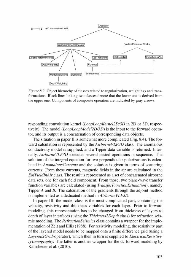
Operator

QuadraticLinearOperator VerticalOperatorBlocks

Damping

FlatnessDataWeighting

ModelWeighting

FlatnessND SmoothnessND

Smoothness

DepthWeighting

LogTransformLogTransformInverse

a D is contained in BD B

Figure 8.2. Object hierarchy of classes related to regularization, weightings and trans-formations. Black lines linking two classes denote that the lower one is derived fromthe upper one. Components of composite operators are indicated by gray arrows.

responding convolution kernel (LoopLoopKernel2D/3D in 2D or 3D, respec-tively). The model (LoopLoopModel2D/3D) is the input to the forward opera-tor, and its output is a concatenation of corresponding data objects.

The situation in paper II is somewhat more complicated (Fig. 8.4). The for-ward calculation is represented by the AirborneVLF3D class. The anomalousconductivity model is supplied, and a Tipper data variable is returned. Inter-nally, AirborneVLF3D executes several nested operations in sequence. Thesolution of the integral equation for two perpendicular polarizations is calcu-lated in AnomalousCurrents and the solution is given in terms of scatteringcurrents. From these currents, magnetic fields in the air are calculated in theEMFieldInAir class. The result is represented as a set of concatenated airbornedata sets, one for each field component. From those, two plane-wave transferfunction variables are calculated (using TransferFunctionEstimation), namelyTipper A and B. The calculation of the gradients through the adjoint methodis implemented as a dedicated method in AirborneVLF3D.

In paper III, the model class is the most complicated part, containing thevelocity, resistivity and thickness variables for each layer. Prior to forwardmodeling, this representation has to be changed from thickness of layers todepth of layer interfaces (using the Thickness2Depth class) for refraction seis-mic modeling. The RefractionSeismics class contains a wrapper for the imple-mentation of Zelt and Ellis (1988). For resistivity modeling, the resistivity partof the layered model needs to be mapped onto a finite difference grid (using aLayered2Grid-operator), which then in turn is supplied to ElectricalResistivi-tyTomography. The latter is another wrapper for the dc forward modeling byKalscheuer et al. (2010).

103

Variable

LoopLoopData

LoopLoopLineData LoopLoopMapData

LoopLoopKernel2DBlockModel3D

LoopLoopKernel3D

LoopLoopModel2D

LoopLoopModel3D

Operator

VerticalOperatorBlocksQuadraticLinearOperator

LoopLoopForwardSingleConfiguration LoopLoopForward

an A enters BB returns a Ca D is contained in BD B

A BB C

Figure 8.3. Object hierarchy of classes used in paper I. Black lines connect super-classes (top) with their derived sub-classes. Colored arrows denote input and outputrelationships between variable and operator classes, gray arrows denote componentsof composite operators and classes.

The potential field forward modeling in paper IV is comparatively sim-ple. Two cell-based 3D models containing density and susceptibility are con-structed and supplied to the respective gravity and magnetics forward opera-tors. Those are very similar in the sense that they both implement a convolu-tion of the model with a Green’s function (kernel) that is different accordingto the physics.

Implementing an inversionThe implementation of an inversion using the described functionality is doneby a short MATLAB script. As an example, a (slightly simplified) script forresistivity inversion using a cell-based model with flatness regularization anddamping of the model update, as it employed in paper III for comparison withthe layer-based inversion, is shown below. In the first part of the script, dataobjects are constructed from data files and model objects are constructed in ac-cordance. From those, a forward operator object can be created. Next, objectsfor parameter transforms, data weighting and regularization are made. Theseoperator objects are then combined accordingly, so that only one abstract for-ward modeling operator and possibly also only one or two regularization op-erators remain. Next follows a loop containing the actual inversion algorithm.The loop is commonly very short compared to the previous steps, and does notchange much for different inverse problems.

104

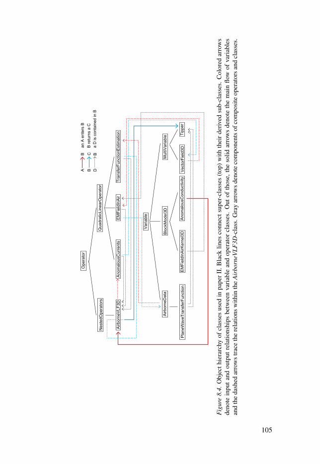
Tran

sfer

Func

tionE

stim

atio

n

Ope

rato

r

Nes

tedO

pera

tors

Qua

drat

icLi

near

Ope

rato

r

Airb

orne

VLF

3DA

nom

alou

sCur

rent

sE

MFi

eldI

nAir

Var

iabl

e

Airb

orne

Dat

aM

ultiV

aria

ble

Pla

neW

aveT

rans

ferF

unct

ion

Tipp

er

Blo

ckM

odel

3D

EM

Fiel

dInA

irKer

nel3

DA

nom

alou

sCon

duct

ivity

Vec

torF

ield

3D

an A

ent

ers

BB

retu

rns

a C

a D

is c

onta

ined

in B

DB

AB

BC

Figu

re8.

4.O

bjec

thie

rarc

hyof

clas

ses

used

inpa

perI

I.B

lack

lines

conn

ects

uper

-cla

sses

(top

)with

thei

rder

ived

sub-

clas

ses.

Col

ored

arro

ws

deno

tein

puta

ndou

tput

rela

tions

hips

betw

een

vari

able

and

oper

ator

clas

ses.

Out

ofth

ose,

the

solid

arro

ws

deno

teth

em

ain

flow

ofva

riab

les

and

the

dash

edar

row

str

ace

the

rela

tions

with

inth

eA

irbo

rneV

LF3D

-cla

ss.G

ray

arro

ws

deno

teco

mpo

nent

sof

com

posi

teop

erat

ors

and

clas

ses.

105

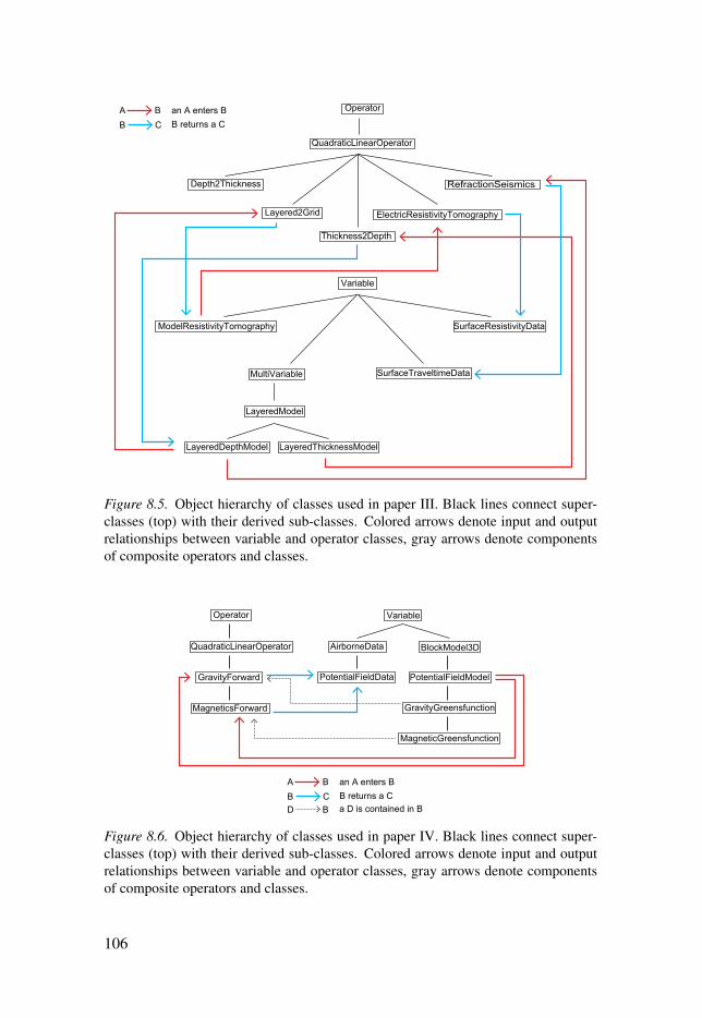
an A enters BB returns a C

A BB C

RefractionSeismics

Operator

QuadraticLinearOperator

ElectricResistivityTomography

Depth2Thickness

Layered2Grid

Thickness2Depth

Variable

SurfaceResistivityData

SurfaceTraveltimeData

ModelResistivityTomography

MultiVariable

LayeredModel

LayeredDepthModel LayeredThicknessModel

Figure 8.5. Object hierarchy of classes used in paper III. Black lines connect super-classes (top) with their derived sub-classes. Colored arrows denote input and outputrelationships between variable and operator classes, gray arrows denote componentsof composite operators and classes.

Operator

QuadraticLinearOperator

GravityForward

MagneticsForward

Variable

AirborneData

PotentialFieldData

BlockModel3D

GravityGreensfunction

MagneticGreensfunction

PotentialFieldModel

an A enters BB returns a Ca D is contained in BD B

A BB C

Figure 8.6. Object hierarchy of classes used in paper IV. Black lines connect super-classes (top) with their derived sub-classes. Colored arrows denote input and outputrelationships between variable and operator classes, gray arrows denote componentsof composite operators and classes.

106

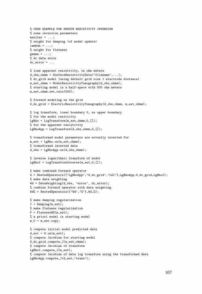
% CODE EXAMPLE FOR SMOOTH RESISTIVITY INVERSION% some inversion parametersmaxiter = ...;% weight for damping (of model update)lambda = ...;% weight for flatnessgamma = ...;% dc data errordc_error = ...

% load apparent resistivity, in ohm metersd_obs_ohmm = SurfaceResistivityData(’filename’,...);% dc_grid model (using default grid size 1 electrode distance)m_est_ohmm = ModelResistivityTomography(d_obs_ohmm);% starting model is a half-space with 500 ohm metersm_est_ohmm.set_vals(500);

% forward modeling on the gridG_dc_grid = ElectricResistivityTomography(d_obs_ohmm, m_est_ohmm);

% log transform, lower boundary 0, no upper boundary% for the model resitivityLgRho = LogTransform(m_est_ohmm,0,[]);% for the apparent resistivityLgRhoApp = LogTransform(d_obs_ohmm,0,[]);

% transformed model parameters are actually inverted form_est = LgRho.on(m_est_ohmm);% transformed inverted datad_obs = LgRhoApp.on(d_obs_ohmm);

% inverse logarithmic transform of modelLgRhoI = LogTransformInverse(m_est,0,[]);

% make combined forward operatorG = NestedOperators(’LgRhoApp’,’G_dc_grid’,’LGI’,LgRhoApp,G_dc_grid,LgRhoI);% make data weightingWd = DataWeighting(d_obs, ’error’, dc_error);% combine forward operator with data weightingWdG = NestedOperators(’Wd’,’G’,Wd,G);

% make damping regularizationI = Damping(m_est);% make flatness regularizationF = FlatnessND(m_est);% a priori model is starting modelm_0 = m_est.copy;

% compute initial model predicted datad_est = G.on(m_est);% compute Jacobian for starting modelG_dc_grid.compute_J(m_est_ohmm);% compute Jacobian of transformLgRhoI.compute_J(m_est);% compute Jacobian of data log transform using the transformed dataLgRhoApp.compute_J(d_est,’trans’);

107

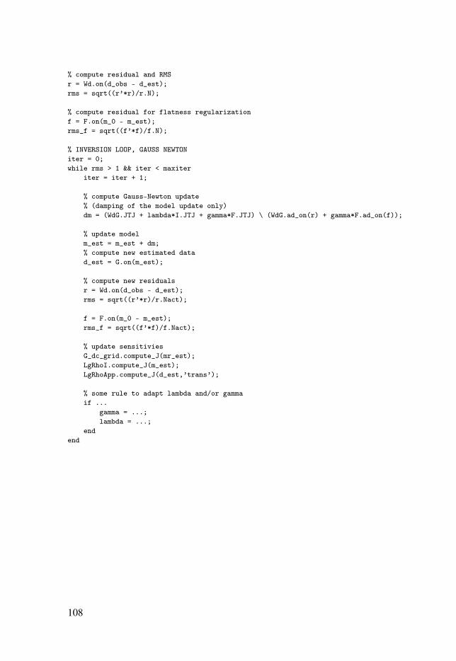
% compute residual and RMSr = Wd.on(d_obs - d_est);rms = sqrt((r’*r)/r.N);

% compute residual for flatness regularizationf = F.on(m_0 - m_est);rms_f = sqrt((f’*f)/f.N);

% INVERSION LOOP, GAUSS NEWTONiter = 0;while rms > 1 && iter < maxiter

iter = iter + 1;

% compute Gauss-Newton update% (damping of the model update only)dm = (WdG.JTJ + lambda*I.JTJ + gamma*F.JTJ) \ (WdG.ad_on(r) + gamma*F.ad_on(f));

% update modelm_est = m_est + dm;% compute new estimated datad_est = G.on(m_est);

% compute new residualsr = Wd.on(d_obs - d_est);rms = sqrt((r’*r)/r.Nact);

f = F.on(m_0 - m_est);rms_f = sqrt((f’*f)/f.Nact);

% update sensitiviesG_dc_grid.compute_J(mr_est);LgRhoI.compute_J(m_est);LgRhoApp.compute_J(d_est,’trans’);

% some rule to adapt lambda and/or gammaif ...

gamma = ...;lambda = ...;

endend

108

Acta Universitatis UpsaliensisDigital Comprehensive Summaries of Uppsala Dissertationsfrom the Faculty of Science and Technology 1116

Editor: The Dean of the Faculty of Science and Technology

A doctoral dissertation from the Faculty of Science andTechnology, Uppsala University, is usually a summary of anumber of papers. A few copies of the complete dissertationare kept at major Swedish research libraries, while thesummary alone is distributed internationally throughthe series Digital Comprehensive Summaries of UppsalaDissertations from the Faculty of Science and Technology.

Distribution: publications.uu.seurn:nbn:se:uu:diva-215673

ACTAUNIVERSITATIS

UPSALIENSISUPPSALA

2014