IEEE TRANSACTIONS ON GEOSCIENCE AND REMOTE SENSING, VOL. 57, NO. 4, APRIL 2019 2075

Joint Petrophysical and Structural Inversion ofElectromagnetic and Seismic Data Based

on Volume Integral Equation MethodTian Lan, Na Liu , Member, IEEE, Feng Han , Member, IEEE, and Qing Huo Liu , Fellow, IEEE

Abstract— A joint petrophysical and structural inversionmethod for electromagnetic (EM) and seismic data based onthe volume integral equation (VIE) is proposed in this paper.In the forward EM problem, only the contrast of conductivity issolved by the electric field integral equation method. However,in the forward seismic problem, both the contrasts of velocity andmass density are solved by the combined field VIE method. Bothforward solvers are accelerated by the fast Fourier transform.In the inversion problem, by using the petrophysical equationsabout the porosity and saturation and applying the chain rule,we fuse the EM and seismic data and construct the jointpetrophysical inversion equations, which can be solved by thevariational Born iteration method. Then, in order to furtherenhance the reconstructed results of the joint petrophysicalinversion, we enforce the structural similarity constraint betweenporosity and water saturation and add the cross-gradient functionto the joint petrophysical inversion cost function. Two typicalgeophysical models based on the remote sensing measurementare used to validate the proposed methods. One is the cross-wellmodel, and the other is the marine surface exploration model.The advantage of the joint inversion compared with the separateinversion is evaluated based on the resolution and the data misfitsof the reconstructed profiles as well as the antinoise ability.

Index Terms— Joint inversion, petrophysical, structuralsimilarity, variational Born iteration method (VBIM).

I. INTRODUCTION

ELECTROMAGNETIC (EM) and seismic full-waveforminversions play an important role in geophysical explo-

ration and reservoir monitoring [1]–[3]. Due to their ownadvantages and disadvantages, these two methods areemployed in different scenes. EM data are mainly used toinvert for the conductivity distribution in the undergroundregion [4], which is widely adopted in metal mine and groundwater detection. However, the propagation of low-frequencyEM wave in the earth is diffusive and suffers from highattenuation. The reconstructed conductivity profile has a lowimage resolution. On the contrary, seismic waves in the earth

Manuscript received April 23, 2018; revised August 18, 2018; acceptedSeptember 16, 2018. Date of publication October 9, 2018; date of currentversion March 25, 2019. This work was supported by the National NaturalScience Foundation of China under Grant 41390453, Grant 11501481, andGrant 41504120. (Corresponding authors: Feng Han; Qing Huo Liu.)

T. Lan, N. Liu, and F. Han are with the Department of ElectronicScience, Institute of Electromagnetics and Acoustics, Xiamen University,Xiamen 361005, China (e-mail: feng.han@xmu.edu.cn).

Q. H. Liu is with the Department of Electrical and Computer Engineering,Duke University, Durham, NC 27708 USA (e-mail: qhliu@duke.edu).

Color versions of one or more of the figures in this paper are availableonline at http://ieeexplore.ieee.org.

Digital Object Identifier 10.1109/TGRS.2018.2871075

have little attenuation, thus seismic inversion results havemuch higher structural resolution than EM inversion results.Unfortunately, the seismic method lacks the ability to discernoil from water, which is an important issue in geophysicalresource exploration. By contrast, due to the high contrastof the conductivity of water and oil, EM fields play anindispensable role to identify the fluid type. Conventionally,these two inversion processes are performed individually, andthe inversion results are finally analyzed simultaneously toexplain the underground structural and conducting informa-tion. Therefore, the joint inversion of EM and seismic data isof great concern to researchers.

The idea of the joint inversion was first proposed in [5]and acquired a great development in the following decades.There are mainly two types of joint inversion methods. Oneis to invert for the petrophysical parameters [6]–[8], such asporosity and fluid saturations, to link different geophysicalparameters, like conductivity in EM problems and velocityand mass density in seismic problems. The links are based onpetrophysical equations. For example, Archie’s equation [9]and Waxman and Smits’ equation [10] build the relation-ships between porosity, water saturation, and conductivity.Gassmann’s equations [11] realize the relationship betweenvelocity, mass density, porosity, and fluid saturations. Thepetrophysical relationships can be obtained by the core analy-sis in the exploration region. Although the petrophysicalequations are empirical and problem-dependent [12], they arewidely adopted in geophysical engineering due to their strongconstraint and good performance. The update of the inverseparameters is simultaneous in this petrophysics-based jointinversion. The second joint inversion method is based on theassumption that there is a structural similarity between thedifferent physical parameters [12]–[14], which is reasonablein the real world. By using the cross-gradient function tolink different physical fields [13], the structures of differ-ent parameters in the same geology will be kept similarwhen the cross-gradient function is minimized. Different fromthe petrophysics-based method, the constraint by the struc-tural similarity is weak. Because the joint structural inver-sion method is more general and problem-independent [15],it can be easily applied to various kinds of physicalscenes [16], [17]. There are two types of updating fashions forthe joint structural inversion. One is alternating [12], and theother is simultaneous [15]. On the one hand, the alternatingfashion has less computation and memory storage than the

0196-2892 © 2018 IEEE. Personal use is permitted, but republication/redistribution requires IEEE permission.See http://www.ieee.org/publications_standards/publications/rights/index.html for more information.

2076 IEEE TRANSACTIONS ON GEOSCIENCE AND REMOTE SENSING, VOL. 57, NO. 4, APRIL 2019

simultaneous fashion. On the other hand, simultaneous inver-sion is more robust [15]. Our previous research is based onthe structural similarity [18], in which the variational Borniteration method (VBIM) is used to reconstruct the contrastsof velocity and conductivity in the 2-D layered media by thealternating fashion. However, the petrophysical parameters arenot considered.

In this paper, we fuse the joint petrophysical and structuralinversions by constructing a unified cost functional basedon the volume integral equation (VIE) method. The directinversion parameters are the porosity and fluid saturations.In the full-waveform inversion process, the 2-D EM forwardscattering problem is formulated by electric field integralequation (EFIE) in layered media with only the contrast ofconductivity taken into account [19]. But for 2-D seismicforward scattering, both the compressibility contrast and massdensity contrast are included in the VIE [20]. The forwarditerations for the EM and seismic scattering are achievedby the stabilized biconjugate gradient (BCGS) method andaccelerated with the fast Fourier transform (FFT) [21]. How-ever, in the inversion process, the petrophysical parametersare retrieved jointly by the VBIM. The update of the directinversion parameters is carried out through the chain rule,which links the original VBIM equation and the variationof petrophysical equations. Then, the minimization process iscarried out by conjugate gradient (CG) method. Consideringthe natural range of the porosity and fluid saturations, we intro-duce the nonlinear transform in VBIM to constrain the rangesof these two parameters during the inversion process [22].Furthermore, we take the cross-gradient function into consid-eration to enforce the structure similarity between porosityand saturation and adopt the simultaneous updating fashion.The inversion results from synthetic data with two typicalgeophysical models are used to evaluate the performance ofthe separate inversion and joint inversion.

This paper is organized as follows. In Section II, we firstintroduce methods for forwarding EM and seismic scatteringcomputation based on VIEs. Then, separate inversions of EMand seismic data are discussed. Joint petrophysical inversionwhich can be further enhanced by enforcing the structuralsimilarity constraint between porosity and water saturation ispresented in Sections II-C and II-D. In Section III, we test theperformance of joint inversion methods as well as separateinversion methods with two geophysical models based on theremote sensing measurement, which are illustrated in Fig. 1.One is the cross-well model, and the other is the marine sur-face exploration model. Finally, conclusions and discussionsare presented in Section IV.

II. METHODS

A. Forward ModelIn the 2-D problem, we define the computational domain �

in the xz plane and assume all the parameters are invariantalong the y direction. The electrical excitation source is alongthe y direction, i.e., only the y direction (TMy) wave is con-sidered. When the transverse magnetic referring to the TMywave propagates, the electric field exists only in y direction,while the magnetic field exists in both x and z directions.

Fig. 1. Illustration of remote sensing measurements in two typical models.(a) Cross-well model, in which the transmitter and receiver are located in thetwo boreholes. (b) Marine surface exploration model, in which the transmitterand receiver are located near the seafloor.

For the EM problem, the scalar Helmholtz equation deducedfrom Maxwell’s equations is�

�+ k2EM

�Ey = jωEMμ0 Jy (1)

where ωEM is the EM angular frequency, μ0 is the per-meability in free space, Jy is the EM source, and kEM =ωEM(μ0�)

1/2 represents the complex wavenumber of the EMfield. We use σ expressing conductivity and � expressing thereal permittivity. Considering σ/ωEM � � in low-frequencygeophysical application, the complex permittivity is

� = � + σ

jωEM≈ σ

jωEM. (2)

For the seismic problem, the scalar acoustic approximationis used, which shows well-posedness in inverse problems [23].Unlike our previous work [18], we no longer neglect thecontrast of mass density ρ in this paper. The acoustic waveequation in frequency domain for scalar pressure p is [24]

∇ · ρ−1∇ p + ω2s κp = −S (3)

where ωs is the acoustic angular frequency, κ is the compress-ibility, and S is the source term. The relationships of κ , ρ,velocity c, and bulk modulus K are

κ = 1/K (4)

K = ρc2. (5)

As we discussed in [20], the wave scattering problem inlayered media can be formulated by the VIE. The total fieldis split into the incident and scattered field. The VIEs ingeneral have no analytic solutions. They are first expanded

LAN et al.: JOINT PETROPHYSICAL AND STRUCTURAL INVERSION OF EM AND SEISMIC DATA BASED ON VIE METHOD 2077

by a set of basis functions and then solved numerically. Thetraditional method of moments (MoM) is not always adoptedto solve the discretized VIEs due to its high computationcost [25]. The computational complexity of MoM for CPUtime is O(N3), and the memory requirement is O(N2), whereN is the number of unknowns in the computation domain.In contrast, the iteration solver BCGS expedited by FFTonly needs O(M N log N) CPU time and O(N) memory [26],where M is the number of iterations.

For the reason that the mass density ρ is considered, (3)in this paper is different from (2) in [18]. Therefore, the VIEused to solve (3) in this paper is different from the EFIE usedto solve (2) in [18]. In order to clarify the difference, we firstgive the analogy of (3) in the EM problem. When both thecontrasts of permittivity and permeability in the EM scatteringproblem are considered, the 2-D Helmholtz equation is [27]

∇ · μ−1∇Ey + ω2�Ey = jωJy. (6)

Comparing (3) with (6), we find that ρ and κ in (3) areanalog of the permeability μ and the permittivity � in (6),respectively. The unknown p in (3) is similar as the unknownEy in (6). We have used the combined field VIE (CFVIE)method to solve the EM scattering problems with both thecontrasts of permittivity and permeability in [20]. Therefore,all the methods in [20] can be applied to solve p in (3).The particle velocity v in acoustics is corresponding to H in2-D EM scattering problem solved by CFVIE.

B. Separate Inversion

VBIM based on the integral equation is first pro-posed in [28] and employed widely in geophysical inver-sion [18], [29], [30]. VBIM takes the variation of the scatteredfield about the contrast and minimizes the cost function toupdate the inverse parameters [29].

For the EM model, the scattered electric field in thereceivers is scalar and can be expressed as

Esct(r) =��

GEJ(r, r�)χ�(r�)E(r�)dr�. (7)

Because of the approximation in (2), the contrast ofpermittivity in (7) can be defined as

χ� = σ − σb

σb(8)

where σ is the conductivity in the computational domain, andσb is the conductivity of the background medium. GEJ isthe 2-D Green’s function in homogeneous or layered media.Its derivation has been discussed in [19]. χ�(r�)E(r�) is actu-ally the equivalent electric current source in the computationaldomain �.

For the seismic model, the scattered pressure field in thereceivers is expressed as

psct(r) =��

G pSκ (r, r�)χκ(r�)p(r�)dr�

−��

GpSρ (r, r�)χρ(r�)v(r�)dr� (9)

where the contrast of compressibility is defined as

χκ = κ − κb

κb(10)

and the contrast of mass density is

χρ = ρ − ρb

ρb. (11)

In (9), G pSκ and GpSρ are the 2-D Green’s functions forseismic wave which are analogous to GEJ and GHM in EMproblems. G pSκ denotes the pressure field generated by theequivalent source χκ(r�)p(r�), while GpSρ means the pressurefield generated by the equivalent source χρ(r�)v(r�).

We take the variation of (7) and (9) about the contrasts andobtain

δEsct(r) =��

GEJ(r, r�)E(r�)δχ�(r�)dr� (12)

δpsct(r) =��

G pSκ (r, r�)p(r�)δχκ(r�)dr�

−��

GpSρ (r, r�)v(r�)δχρ(r�)dr� (13)

where E , p, and v are the total fields in the forward computa-tion. This is different from our previous work [18], in whichthe incident fields are used to approximate the total fields,i.e., the Born approximation is adopted [18], [29]. The Bornapproximation is only suitable for weak scattering. In thispaper, we directly use the total fields in (12) and (13). Conse-quently, the strong scattering problems can also be computed.δEsct and δpsct are the misfits of the scattered fields betweenthe measured data and the computed data similar to that inour previous work [18]. The inversion process in the VBIM isto obtain δχ� as well as δχκ and δχρ by minimizing the costfunction, which is defined as

Fq (δχq)=∥∥δfsct

q−1−Lq−1δχq

∥∥2+γ 2

∥∥δfsctq−1

∥∥2

�δχq−1�2 �δχq�2 (14)

where � · � means the L2 norm, q is the iteration index,fsct is the scattered electric field or scattered pressure field,γ is the fixed regularization factor, and χ is the contrastwhich can be χ � or the combination of χκ and χρ . In eachiteration, we compute the scattered field from the newestinverted parameters. Then, we update δfsct

q−1 by subtractingthe computed scattered field from the measured scattered field.�δfsct

q−1�2/�δχq−1�2 is the self-adaptive regularization factor,which can decrease along with the inversion process accordingto the change of δfsct and δχ in the previous step. The leastsquare problem of (14) is transformed into [18]

⎛⎝L†

q−1Lq−1 + γ 2��δfsct

q−1

��2

�δχq−1�2 I

⎞⎠ δχq = L†

q−1δfsctq−1 (15)

where † means the complex conjugate and transpose operation.This equation can be solved by the CG method [31] toobtain δχq . Once δχq is obtained, we update χ and performthe forward computation to compute the total field E in (12),and p and v in (13). Then, fsct

q and Lq in (15) can beupdated to obtain δχq+1. Because the inverse parameters are

2078 IEEE TRANSACTIONS ON GEOSCIENCE AND REMOTE SENSING, VOL. 57, NO. 4, APRIL 2019

not frequency-dependent, the iteration can be easily appliedfor the simultaneous multifrequency inversion.

Note that there are four criteria to terminate the iteration inthe inversion process by VBIM as follows.

1) Data misfit is less than the threshold.2) Decrease of data misfit between two iterations is smaller

than a threshold.3) The data misfit in the latest iteration is bigger than the

previous one.4) The change of inversion parameters is smaller than a

threshold.To quantitatively evaluate the performance of inversion,

we define the model misfit as

Errmodel = �minv − mtrue��mtrue� (16)

where minv is the inverted parameter in the discretized compu-tational domain, and mtrue is the true parameters distributionin that region.

We also define the data misfit as

Errdata =��fsct

inv − fsctmeas

����fsctmeas

�� (17)

where fsctinv in the receivers is the scatted field computed from

the inverted parameter minv, and fsctmeas is the scattered field

from measurement.

C. Joint Petrophysical InversionFor joint petrophysical inversion, we build relationships

between geophysical parameters and petrophysical parame-ters based on the petrophysical equations. In the following,we will see that the petrophysical parameters can determinethe geophysical parameters uniquely, while geophysical para-meters can match countless compositions of the petrophysicalparameters.

For the EM parameter, we adopt Archie’s equation [8], [9]

σ = 1

aσwφ

m Snw (18)

where σw is the conductivity of the formation saline water,a is the tortuosity factor, φ is the porosity, m is the exponentof porosity, Sw is the water saturation, and n is the exponent ofsaturation. Then, we have the variational expression about (18)

δσ = 1

aσw�mφm−1Sn

wδφ + nφm Sn−1w δSw

�. (19)

For seismic parameters, we use Gassmann’s equa-tions [8], [11]. In virtue of the acoustic approximation,we only consider compressional wave (P-wave) and neglectthe shear modulus in this paper. In this case, we assume anoil–water system. The gas saturation Sg is omitted. Therefore,Gassmann’s equations are given as

K = (1 − β)Kma + β2M (20a)

M =�β − φ

Kma+ φ

K f

�−1

(20b)

K f =�

CwSwKw

+ CoSo

Ko

�−1

(20c)

ρ = (1 − φ)ρma + φ(Swρw + Soρo) (20d)

where So = 1.0−Sw is the oil saturation, Kma and ρma are thebulk modulus and the density of the matrix (solid or grain),Kw is the bulk modulus for water, and Ko is the bulk modulusfor oil. Cw and Co are correction terms for water and oil, whichare usually equal to 1 [15]. The Biot coefficient β satisfies

β =�φ/φc, 0 ≤ φ ≤ φc

1, φ > φc(21)

where φc is the critical porosity. We also make the variationof (20) about φ and Sw

δK =φβ2 M2

�Co

Ko− Cw

Kw

�δSw

+�

2βM − Kma − β2 M2

Kma

�∂β

∂φδφ

− β2M2�

1

K f− 1

Kma

�δφ (22a)

δρ = (Swρw + Soρo − ρma)δφ + φ(ρw − ρo)δSw (22b)

where ∂β/∂φ is

∂β

∂φ=�

1/φc, 0 ≤ φ ≤ φc

0, φ > φc.(23)

The last step is to obtain the variational expressions of(4), (8), (10), and (11)

δκ = − 1

K 2 δK (24)

δχ� = 1

σbδσ (25)

δχκ = 1

κbδκ (26a)

δχρ = 1

ρbδρ. (26b)

Combining (12), (19), and (25) with the chain rule, we canobtain the variational equation of the scattered electric fieldabout porosity and water saturation, which is expressed in thediscrete form with matrix

δEsctq−1 = LEM

q−1

δφδSw

. (27)

By following the similar procedure, we combine (13), (22),(24), and (26) and obtain the discrete form of the variationalequation of the scattered pressure field about porosity andwater saturation, which is expressed as

δpsctq−1 = LS

q−1

δφδSw

. (28)

We can assemble (27) and (28) directly, and then the jointvariational equation including EM and seismic data is

δEsctq−1

ηδpsctq−1

=�

LEMq−1 ηLS

q−1

� δφδSw

(29)

where the joint petrophysical factor η is defined as

η =��δEsct

q−1

����δpsctq−1

�� (30)

LAN et al.: JOINT PETROPHYSICAL AND STRUCTURAL INVERSION OF EM AND SEISMIC DATA BASED ON VIE METHOD 2079

to balance the contribution of different fields during theinversion process.

We express (29) compactly as

δfsctq−1 = Lq−1δψ . (31)

Next, similar to (14), the cost function in the jointpetrophysical inversion is defined as

Fq(δψq) = ∥∥δfsctq−1 − Lq−1δψq

∥∥2 + γ 2

∥∥δfsctq−1

∥∥2

�δψq−1�2 �δψq�2.

(32)

The least square problem of (32) is transformed into⎛⎝L†

q−1Lq−1 + γ 2��δfsct

q−1

��2

�δψq−1�2 I

⎞⎠ δψq = L†

q−1fsctq−1. (33)

This equation can also be solved by the CG method as (15).Because the elements in the matrix of the left side and thosein the vector of right side of (33) are complex numbers,the solution space of CG is in the complex number domain.However, the porosity and water saturation are real physicalvariables. Therefore, we can decouple the real and imaginaryparts of (33) and reassemble the equation as

Aδψq = b (34)

where

A =

⎛⎜⎜⎜⎜⎝

Re

�L†

q−1Lq−1 + γ 2��δfsct

q−1

��2

�δψq−1�2 I

�

Im

�L†

q−1Lq−1 + γ 2��δfsct

q−1

��2

�δψq−1�2 I

�⎞⎟⎟⎟⎟⎠ (35)

b =�

Re�L†

q−1fsctq−1

�Im�L†

q−1fsctq−1

��. (36)

During the inversion process, we introduce the nonlineartransform to constrain the inverse parameter within a rea-sonable range. For the VBIM in this paper, this nonlineartransform and the corresponding inverse transform are [22]

ψ = ψmin + ψmax exp(ψ)

1 + exp(ψ)(37)

and

ψ = log(ψ − ψmin)− log(ψmax − ψ) (38)

respectively, where ψmin is the lower limit while ψmax is theupper limit. The variational equation for (37) is

δψ = (ψmax − ψmin) exp(ψ)

[1 + exp(ψ)]2 δψ. (39)

By this transform, the inverse parameters ψ are always con-strained between ψmin and ψmax. Therefore, the unreasonableinversion results are avoided.

D. Joint Structural InversionIn the previous work [18], we build a cross-gradient func-

tion for χ� and χc and use the alternative fashion in EMand seismic VBIM joint inversion iteration. By enforcingthe structural similarity between different inverse parameters,the poor inverted profile of one parameter can be improvedby the good resolution of the other parameter [32]. Here,we adopt the similar strategy and also build a cross-gradientfunction for φ and Sw

t = ∇φ × ∇Sw (40)

where × is the outer product operation. When the cross-gradient function is minimized, the two edges in the profile ofdifferent inverse petrophysical parameters are aligned alongthe same orientation. Because φ and Sw range from 0 to 1without units, it is unnecessary to normalize inverse parametersas in [12]–[14]. The element of the cross-gradient function canbe discretized with the central difference method [18]

ti, j =�φi, j+1 − φi, j−1

2�z

��Sw;i+1, j − Sw;i−1, j

2�x

�

−�φi+1, j − φi−1, j

2�x

��Sw;i, j+1 − Sw;i, j−1

2�z

�. (41)

As in [18], we expand t with first-order Taylor series aroundtq−1 and neglect the high-order term

tq(ψq )∼= tq−1(ψq−1)+ Bq−1δψq . (42)

Then, the cost function (32) is added with the cross-gradientfunction (42)

Fq (δψq) = ∥∥δfsctq−1 − Lq−1δψq

∥∥2 + γ 2

∥∥δfsctq−1

∥∥2

�δψq−1�2 �δψq�2

+w2

��δfsctq−1

��2

�tq−1�2 �tq−1 + Bq−1δψq�2 (43)

where w is the joint structural factor. Finally, this jointpetrophysical and structural cost function is transformed toa form⎛⎝L†

q−1Lq−1 + γ 2��δfscat

q−1

��2

�δψq−1�2 I + w2∥∥δfsct

q−1

∥∥2

�tq−1�2 B†q−1Bq−1

⎞⎠ δψq

= L†q−1δf

sctq−1 − w2

��δfsctq−1

��2

�tq−1�2 B†q−1tq−1 (44)

which is also solved by the CG method. It should be notedthat the simultaneous updating fashion will be used in thispaper. Therefore, (43) is different from the cost function usedfor alternative updating fashion presented in our previouswork [18].

III. NUMERICAL ASSESSMENT

In this section, we will use two typical models to evaluatedifferent inversion methods. Both models are common in geo-physical application engineering and widely used in geophysi-cal inversion method evaluations. One model is the cross-wellmeasurement, in which the transmitters and receivers arelocated in the two wells. The other is the marine surface

2080 IEEE TRANSACTIONS ON GEOSCIENCE AND REMOTE SENSING, VOL. 57, NO. 4, APRIL 2019

Fig. 2. Cross-well model. (a) Porosity distribution. (b) Water saturationdistribution. There are 16 transmitters and 16 receivers located in the twoboreholes locating at x = 40 m and x = 560 m, respectively. The transmittersdistribute uniformly from z = 1125 m to z = 2175 m. The receivers distributeuniformly from z = 1050 m to z = 2100 m.

exploration model, in which the transmitters and receivers arelocated near the seabed. In all inversion processes mentionedbelow, we use the nonlinear transform (37) to constrain theinversion petrophysical parameters. For porosity, the con-strained range is 0–0.35. For water saturation, the range is 0–1.The fixed regularization factor γ in (32) is chosen as 0.3.We use the initial model with the porosity and water saturationwhich are 0.01 larger than the background parameters.

A. Cross-Well ModelFig. 2 shows the petrophysical distribution of a typical

cross-well model. Several reservoirs with different shapesare located between two boreholes. The background of themodel is homogeneous. The porosity φ is 0.1, and the watersaturation Sw is 0.3.

We assume the petrophysical parameters of reservoirs areφ = 0.2 and Sw = 0.5. The other petrophysical constants inthe petrophysical equations (18) and (20) are mainly referredto [8]. The Archie’s constants are a = 1, σw = 5.5 S/m,m = 1.2, and n = 2.0. Gassmann’s constant are φc = 0.4,ρma = 2560 kg/m3, ρw = 1050 kg/m3, ρo = 750 kg/m3,Kma = 32 Gpa, Kw = 2.81 Gpa, and Ko = 0.75 Gpa.There are total 16 transmitters and 16 receivers situated in twoboreholes, which are even spaced with the interval of 150 m.We use single-frequency data in this model. The EM frequencyis 100 Hz, and the seismic frequency is 15 Hz. The inversiondomain is 500 m × 1000 m, which is discretized withuniform square cells. The cell size is 5 × 5 m2, and thusthe cell number is 100 × 200. Unlike finite difference-basedinversion methods [8], [15], we do not need the perfectmatching layerlike boundary condition in VIE-based inversionmethod. Hence, there is no need to expand the computationaldomain.

First, we perform the EM-only inversion, i.e., we only applythe VBIM to (27) to reconstruct the porosity and saturationdistribution in the cross-well model. After five iterations,the data misfit is 2.80% and almost keeps unchanged, so theVBIM terminates. The results are shown in Fig. 3(a) and (e).We can see the water saturation in the inversion results iscloser to the true value than the porosity. This phenomenon is

due to the fact that the EM data is more sensitive to the watersaturation than to the porosity [8].

Similarly, we perform the inversion using only the seismicdata, and the results are shown in Fig. 3(b) and (f). The inver-sion terminates after five iterations and the seismic data misfitis 0.67%. Compared with the results in EM-only inversion,the profile of porosity in seismic-only inversion has a muchbetter resolution and is closer to the true model. However,the water saturation results are far away from the true values.The reason is that the seismic data is less sensitive to the watersaturation compared with the porosity. Individual EM-only orseismic-only inversion cannot recover well the porosity andsaturation simultaneously.

Then, we use the joint petrophysical inversion, i.e., apply theVBIM algorithm to (29), to enhance the quality of the recon-structed profiles. The results are shown in Fig. 3(c) and (g).After the VBIM inversion finishes five iterations, the datamisfit for the scattered EM field is 0.75% and 0.48% forthe seismic field. Compared with the results of the separateinversions shown in Fig. 3(a), (b), (e), and (f), not only theresolution of the reconstructed profiles is improved but alsothe values of the porosity and water saturation are closer tothe true values. We quantify the model misfits of differentinversion methods and list the results in Table I. The misfitsof the porosity and saturation are both reduced by joint petro-physical inversion. We then further reduce the model misfits byenforcing the structural similarity constraint between porosityand water saturation in the joint inversion. The inverted profilesof joint petrophysical and structural inversion are shown inFig. 3(d) and (h). The data misfit variations versus iterationsteps for different inversion processes are shown in Fig. 5.We can see that the convergence is fast in all inversionprocesses.

Finally, the antinoise ability of different inversion algo-rithms is tested. We add Gaussian random white noises in thedata of the measured scattered field. The effects of differentsignal-to-noise ratios (SNRs) are tested. The model misfitchanges along with the different SNR values are shownin Fig. 6. We can see the model misfit increases with thedecrease of SNR. We also note that the model misfits inthe joint petrophysical with the structural similarity constraintare always smaller than misfits without the constraint. Themodel misfits for EM-only and seismic-only inversions whenthe noise is added are obviously larger than the misfits forjoint inversions shown in Fig. 6 and thus are not displayed.The inversion results when SNR = 1 dB are shown in Fig. 4.We can see that the main reservoirs are still discernable andthe small reservoirs become blur when the noise is too big. Thejoint petrophysical and structural inversion has the strongestantinoise ability.

B. Marine Surface Exploration ModelFor the marine surface exploration model, we use the

constants mainly referred to [15] in petrophysical equations(18) and (20). a = 1, σw = 3.0, m = 0.4, n = 2.4, φc = 0.4,ρma = 2560 kg/m3, ρw = 1050 kg/m3, ρo = 750 kg/m3,Kma = 37 Gpa, Kma = 2.56 Gpa, and Kma = 0.75 Gpa.As shown in Fig. 7, the upper layer is seawater, whose porosity

LAN et al.: JOINT PETROPHYSICAL AND STRUCTURAL INVERSION OF EM AND SEISMIC DATA BASED ON VIE METHOD 2081

Fig. 3. Inversion results for the cross-well model when noise free. Reconstructed distributions of (a) porosity and (e) water saturation using only EM data.Reconstructed distributions of (b) porosity and (f) water saturation using only seismic data. Reconstructed distributions of (c) porosity and (g) water saturationusing both EM and seismic data. Reconstructed distributions of (d) porosity and (h) water saturation using both EM and seismic data with structural constraint.

TABLE I

MODEL MISFITS FOR DIFFERENT INVERSION METHODS

IN CROSS-WELL MODEL WHEN NOISE FREE

is 1.0 and water saturation is 1.0. The middle layer is theseawater intrusion zone with the thickness of 400 m, whoseporosity is 0.3 and water saturation is 1.0. The lower layeris the crust, whose porosity is 0.1 and water saturation is0.8. Green’s function in layered medium is used. There are40 transmitters and 40 receivers located near the seabedat z = 100 m. The transmitters and receivers are placedalternately with the interval of 300 m. We use the mul-tifrequency simultaneous inversion in this model. We pickEM frequency of 0.4 and 0.8 Hz, and seismic frequency of0.4, 0.8, 1.2, and 1.6 Hz. The inversion domain in the lower

layer is 10 km × 4 km, and discretized with 250 × 100 cells.The cell size is 40 × 40 m2.

First, we invert the EM-only data for this model. Afterthree inversion iterations, the EM data misfit is 0.97%. Theresults are shown in Fig. 8(a) and (b). Due to the diffusivecharacteristic of EM wave, the resolution is poor. Consistentwith the reason that the EM data are more sensitive to thewater saturation, the reconstructed profile of water saturationis better than that of porosity.

Then, we only use seismic data to obtain the petrophysicaldistribution and the results are shown in Fig. 8(c) and (d).In the inversion iteration, when the data misfit approach-ing 2.90%, it almost keeps unchanged any more. Thus,the inversion process is stopped. The inverted profile ofporosity matches well with the true model. We can see thatthe resolution in the porosity profile is better than that inEM-only inversion, which is owing to the little attenuationof seismic wave during propagation. Nevertheless, we have apoor inversion result about the water saturation, because of theweak sensitivity of seismic data for the water saturation.

2082 IEEE TRANSACTIONS ON GEOSCIENCE AND REMOTE SENSING, VOL. 57, NO. 4, APRIL 2019

Fig. 4. Inversion results for the cross-well model when SNR = 1 dB. Reconstructed distributions of (a) porosity and (e) water saturation using only EMdata. Reconstructed distributions of (b) porosity and (f) water saturation using only seismic data. Reconstructed distributions of (c) porosity and (g) watersaturation using both EM and seismic data. Reconstructed distributions of (d) porosity and (h) water saturation using both EM and seismic data with structuralconstraint.

Fig. 5. Inversion convergence process in the cross-well model. (a) EM datamisfits. (b) Seismic data misfits.

Hence, we use the joint petrophysical inversion to improvethe quality of reconstructed profiles. The results are shownin Fig. 8(e) and (f). Compared with the previous inversion withsingle physical data, the recovered resolution and values ofporosity and water saturation are improved obviously. At thistime, the inversion process terminates when the EM data misfitis 0.54% and the seismic data misfit is 5.45%. In addition to

Fig. 6. Model misfits change with the SNR in the cross-well model. Modelmisfits of (a) porosity and (b) water saturation.

the joint petrophysical method, we use structural similarityconstraint to obtain better results shown in Fig. 8(g) and (h).We then compare the model misfits of these inversions andlist the results in Table II. We can see that the model misfitsare reduced by the joint petrophysical inversion and furtherdecreased by introducing the structural constraint, even whenthe joint inversion is terminated with larger data

LAN et al.: JOINT PETROPHYSICAL AND STRUCTURAL INVERSION OF EM AND SEISMIC DATA BASED ON VIE METHOD 2083

Fig. 7. Marine surface exploration model. (a) Porosity distribution. (b) Water saturation distribution. There are 40 transmitters and 40 receivers near theseabed at z = 0.1 km. The transmitters distribute uniformly from x = 0 km to x = 11.7 km. The receivers distribute uniformly from x = 0.3 km to x = 12 km.

Fig. 8. Inversion results for the marine surface exploration model when noise free. Reconstructed distributions of (a) porosity and (b) water saturation usingonly EM data. Reconstructed distributions of (c) porosity and (d) water saturation using only seismic data. Reconstructed distributions of (e) porosity and(f) water saturation using both EM and seismic data. Reconstructed distributions of (g) porosity and (h) water saturation using both EM and seismic data withstructural constraint.

misfits compared with EM-only or seismic-only inversions.The data misfit changes with iterations for different inver-sion processes are shown in Fig. 10. We can see that the

convergence is fast in the first several steps but becomes slowwhen approaching the threshold. However, the convergence isstable in all inversion processes.

2084 IEEE TRANSACTIONS ON GEOSCIENCE AND REMOTE SENSING, VOL. 57, NO. 4, APRIL 2019

Fig. 9. Inversion results for the marine surface exploration model when SNR = 1 dB. Reconstructed distributions of (a) porosity and (b) water saturationusing only EM data. Reconstructed distributions of (c) porosity and (d) water saturation using only seismic data. Reconstructed distributions of (e) porosityand (f) water saturation using both EM and seismic data. Reconstructed distributions of (g) porosity and (h) water saturation using both EM and seismic datawith structural constraint.

TABLE II

MODEL MISFITS FOR DIFFERENT INVERSION METHODS IN MARINESURFACE EXPLORATION MODEL WHEN NOISE FREE

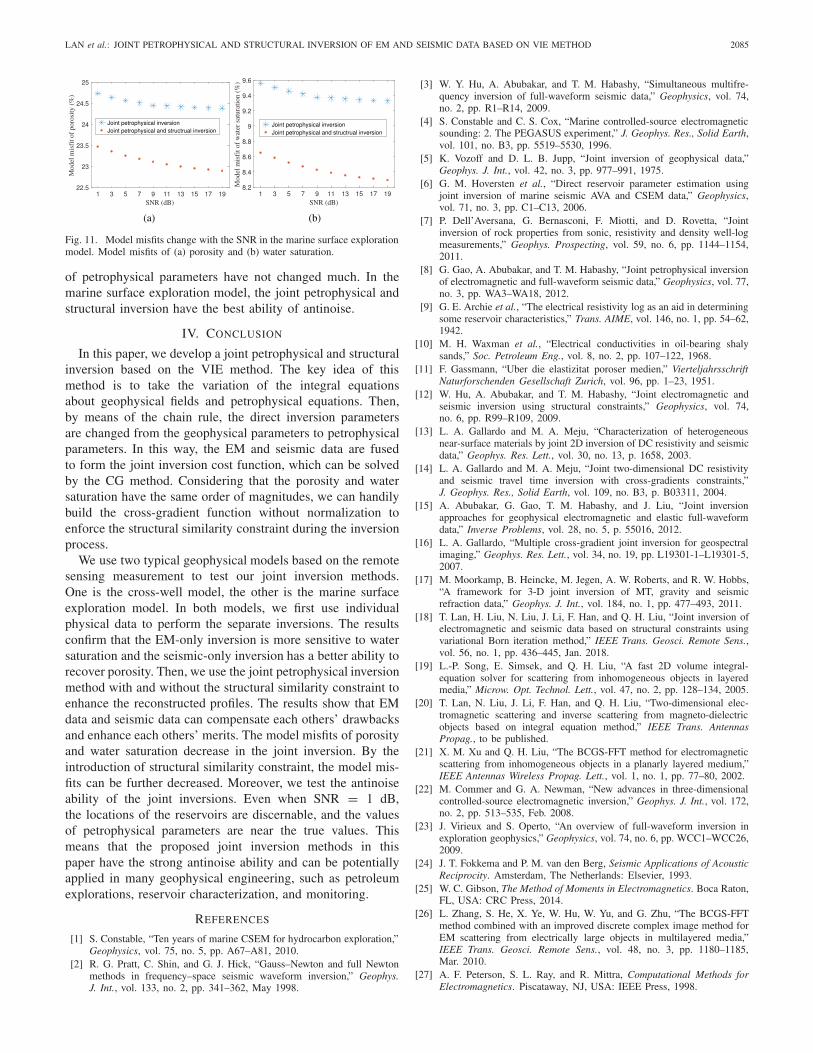
Finally, we also test the effect of noise on the marinesurface exploration model. As in the cross-well model, we use10 different SNR values to implement four types of inver-sions. The model misfit versus SNR by joint inversions isshown in Fig. 11. We can see the model misfit increases asthe noise increases and the performance of joint petrophys-ical and structural inversion is better than that without the

Fig. 10. Inversion convergence process in the marine surface explorationmodel. (a) EM data misfits. (b) Seismic data misfits.

structural constraint. Then, the inversion results when SNR =1 dB are shown in Fig. 9. Compared with the noise-freesituation in Fig. 8, the resolution becomes worse. Nevertheless,the basic information about the location of reservoir and values

LAN et al.: JOINT PETROPHYSICAL AND STRUCTURAL INVERSION OF EM AND SEISMIC DATA BASED ON VIE METHOD 2085

Fig. 11. Model misfits change with the SNR in the marine surface explorationmodel. Model misfits of (a) porosity and (b) water saturation.

of petrophysical parameters have not changed much. In themarine surface exploration model, the joint petrophysical andstructural inversion have the best ability of antinoise.

IV. CONCLUSION

In this paper, we develop a joint petrophysical and structuralinversion based on the VIE method. The key idea of thismethod is to take the variation of the integral equationsabout geophysical fields and petrophysical equations. Then,by means of the chain rule, the direct inversion parametersare changed from the geophysical parameters to petrophysicalparameters. In this way, the EM and seismic data are fusedto form the joint inversion cost function, which can be solvedby the CG method. Considering that the porosity and watersaturation have the same order of magnitudes, we can handilybuild the cross-gradient function without normalization toenforce the structural similarity constraint during the inversionprocess.

We use two typical geophysical models based on the remotesensing measurement to test our joint inversion methods.One is the cross-well model, the other is the marine surfaceexploration model. In both models, we first use individualphysical data to perform the separate inversions. The resultsconfirm that the EM-only inversion is more sensitive to watersaturation and the seismic-only inversion has a better ability torecover porosity. Then, we use the joint petrophysical inversionmethod with and without the structural similarity constraint toenhance the reconstructed profiles. The results show that EMdata and seismic data can compensate each others’ drawbacksand enhance each others’ merits. The model misfits of porosityand water saturation decrease in the joint inversion. By theintroduction of structural similarity constraint, the model mis-fits can be further decreased. Moreover, we test the antinoiseability of the joint inversions. Even when SNR = 1 dB,the locations of the reservoirs are discernable, and the valuesof petrophysical parameters are near the true values. Thismeans that the proposed joint inversion methods in thispaper have the strong antinoise ability and can be potentiallyapplied in many geophysical engineering, such as petroleumexplorations, reservoir characterization, and monitoring.

REFERENCES

[1] S. Constable, “Ten years of marine CSEM for hydrocarbon exploration,”Geophysics, vol. 75, no. 5, pp. A67–A81, 2010.

[2] R. G. Pratt, C. Shin, and G. J. Hick, “Gauss–Newton and full Newtonmethods in frequency–space seismic waveform inversion,” Geophys.J. Int., vol. 133, no. 2, pp. 341–362, May 1998.

[3] W. Y. Hu, A. Abubakar, and T. M. Habashy, “Simultaneous multifre-quency inversion of full-waveform seismic data,” Geophysics, vol. 74,no. 2, pp. R1–R14, 2009.

[4] S. Constable and C. S. Cox, “Marine controlled-source electromagneticsounding: 2. The PEGASUS experiment,” J. Geophys. Res., Solid Earth,vol. 101, no. B3, pp. 5519–5530, 1996.

[5] K. Vozoff and D. L. B. Jupp, “Joint inversion of geophysical data,”Geophys. J. Int., vol. 42, no. 3, pp. 977–991, 1975.

[6] G. M. Hoversten et al., “Direct reservoir parameter estimation usingjoint inversion of marine seismic AVA and CSEM data,” Geophysics,vol. 71, no. 3, pp. C1–C13, 2006.

[7] P. Dell’Aversana, G. Bernasconi, F. Miotti, and D. Rovetta, “Jointinversion of rock properties from sonic, resistivity and density well-logmeasurements,” Geophys. Prospecting, vol. 59, no. 6, pp. 1144–1154,2011.

[8] G. Gao, A. Abubakar, and T. M. Habashy, “Joint petrophysical inversionof electromagnetic and full-waveform seismic data,” Geophysics, vol. 77,no. 3, pp. WA3–WA18, 2012.

[9] G. E. Archie et al., “The electrical resistivity log as an aid in determiningsome reservoir characteristics,” Trans. AIME, vol. 146, no. 1, pp. 54–62,1942.

[10] M. H. Waxman et al., “Electrical conductivities in oil-bearing shalysands,” Soc. Petroleum Eng., vol. 8, no. 2, pp. 107–122, 1968.

[11] F. Gassmann, “Uber die elastizitat poroser medien,” VierteljahrsschriftNaturforschenden Gesellschaft Zurich, vol. 96, pp. 1–23, 1951.

[12] W. Hu, A. Abubakar, and T. M. Habashy, “Joint electromagnetic andseismic inversion using structural constraints,” Geophysics, vol. 74,no. 6, pp. R99–R109, 2009.

[13] L. A. Gallardo and M. A. Meju, “Characterization of heterogeneousnear-surface materials by joint 2D inversion of DC resistivity and seismicdata,” Geophys. Res. Lett., vol. 30, no. 13, p. 1658, 2003.

[14] L. A. Gallardo and M. A. Meju, “Joint two-dimensional DC resistivityand seismic travel time inversion with cross-gradients constraints,”J. Geophys. Res., Solid Earth, vol. 109, no. B3, p. B03311, 2004.

[15] A. Abubakar, G. Gao, T. M. Habashy, and J. Liu, “Joint inversionapproaches for geophysical electromagnetic and elastic full-waveformdata,” Inverse Problems, vol. 28, no. 5, p. 55016, 2012.

[16] L. A. Gallardo, “Multiple cross-gradient joint inversion for geospectralimaging,” Geophys. Res. Lett., vol. 34, no. 19, pp. L19301-1–L19301-5,2007.

[17] M. Moorkamp, B. Heincke, M. Jegen, A. W. Roberts, and R. W. Hobbs,“A framework for 3-D joint inversion of MT, gravity and seismicrefraction data,” Geophys. J. Int., vol. 184, no. 1, pp. 477–493, 2011.

[18] T. Lan, H. Liu, N. Liu, J. Li, F. Han, and Q. H. Liu, “Joint inversion ofelectromagnetic and seismic data based on structural constraints usingvariational Born iteration method,” IEEE Trans. Geosci. Remote Sens.,vol. 56, no. 1, pp. 436–445, Jan. 2018.

[19] L.-P. Song, E. Simsek, and Q. H. Liu, “A fast 2D volume integral-equation solver for scattering from inhomogeneous objects in layeredmedia,” Microw. Opt. Technol. Lett., vol. 47, no. 2, pp. 128–134, 2005.

[20] T. Lan, N. Liu, J. Li, F. Han, and Q. H. Liu, “Two-dimensional elec-tromagnetic scattering and inverse scattering from magneto-dielectricobjects based on integral equation method,” IEEE Trans. AntennasPropag., to be published.

[21] X. M. Xu and Q. H. Liu, “The BCGS-FFT method for electromagneticscattering from inhomogeneous objects in a planarly layered medium,”IEEE Antennas Wireless Propag. Lett., vol. 1, no. 1, pp. 77–80, 2002.

[22] M. Commer and G. A. Newman, “New advances in three-dimensionalcontrolled-source electromagnetic inversion,” Geophys. J. Int., vol. 172,no. 2, pp. 513–535, Feb. 2008.

[23] J. Virieux and S. Operto, “An overview of full-waveform inversion inexploration geophysics,” Geophysics, vol. 74, no. 6, pp. WCC1–WCC26,2009.

[24] J. T. Fokkema and P. M. van den Berg, Seismic Applications of AcousticReciprocity. Amsterdam, The Netherlands: Elsevier, 1993.

[25] W. C. Gibson, The Method of Moments in Electromagnetics. Boca Raton,FL, USA: CRC Press, 2014.

[26] L. Zhang, S. He, X. Ye, W. Hu, W. Yu, and G. Zhu, “The BCGS-FFTmethod combined with an improved discrete complex image method forEM scattering from electrically large objects in multilayered media,”IEEE Trans. Geosci. Remote Sens., vol. 48, no. 3, pp. 1180–1185,Mar. 2010.

[27] A. F. Peterson, S. L. Ray, and R. Mittra, Computational Methods forElectromagnetics. Piscataway, NJ, USA: IEEE Press, 1998.

2086 IEEE TRANSACTIONS ON GEOSCIENCE AND REMOTE SENSING, VOL. 57, NO. 4, APRIL 2019

[28] N. Zaiping, Y. Feng, Z. Yanwen, and Z. Yerong, “Variational Borniteration method and its applications to hybrid inversion,” IEEE Trans.Geosci. Remote Sens., vol. 38, no. 4, pp. 1709–1715, Jul. 2000.

[29] W. Zhang and Q. H. Liu, “Three-dimensional scattering and inversescattering from objects with simultaneous permittivity and permeabil-ity contrasts,” IEEE Trans. Geosci. Remote Sens., vol. 53, no. 1,pp. 429–439, Jan. 2015.

[30] Z. Yu, J. Zhou, Y. Fang, Y. Hu, and Q. H. Liu, “Through-casing hydraulicfracture evaluation by induction logging II: The inversion algorithm andexperimental validations,” IEEE Trans. Geosci. Remote Sens., vol. 55,no. 2, pp. 1189–1198, Feb. 2017.

[31] J. R. Shewchuk et al., “An introduction to the conjugate gradientmethod without the agonizing pain,” Carnegie Mellon Univ., Pittsburgh,PA, USA, Tech. Rep. CMU-CS-94-125, Aug. 1994.

[32] M. Li, L. Liang, A. Abubakar, and P. M. Van Den Berg, “Structuralsimilarity regularization scheme for multiparameter seismic full wave-form inversion,” in Proc. SEG Tech. Program Expanded Abstracts, 2013,pp. 1089–1094.

Tian Lan received the B.S. degree in electro-magnetic fields and wireless technology and theM.S. degree in electromagnetic fields and microwavetechnology from the University of Electronic Sci-ence and Technology of China, Chengdu, China,in 2011 and 2014, respectively. He is currentlypursuing the Ph.D. degree with Xiamen University,Xiamen, China.

His research interests include fast-forward solversin electromagnetics and acoustics and joint inversionmethods in multiphysical fields.

Na Liu (M’18) received the Ph.D. degree in compu-tational mathematics from the University of ChineseAcademy of Sciences, Beijing, China, in 2013.

From 2012 to 2013, she was a Visiting Studentwith the Department of Electrical and ComputerEngineering, Duke University, Durham, NC, USA.From 2013 to 2017, she held a postdoctoral posi-tion with Xiamen University, Xiamen, China, whereshe is currently an Associate Professor with theInstitute of Electromagnetics and Acoustics. Herresearch interests include computational electromag-

netics, especially the fast and efficient methods for complex media and theirapplications in cavities and optical waveguide problems.

Feng Han (M’17) received the B.S. degree inelectronic science from Beijing Normal University,Beijing, China, in 2003, the M.S. degree in geo-physics from Peking University, Beijing, in 2006,and the Ph.D. degree in electrical engineering fromDuke University, Durham, NC, USA, in 2011.

He is currently an Assistant Professor with theInstitute of Electromagnetics and Acoustics, XiamenUniversity, Xiamen, China. His research inter-ests include ionosphere remote sensing by radioatmospherics, electromagnetic full-wave inversion

by integral equations, reverse time migration image, and the design of anelectromagnetic detection system.

Qing Huo Liu (S’88–M’89–SM’94–F’05) receivedthe B.S. and M.S. degrees in physics from XiamenUniversity, Xiamen, China, in 1983 and 1986,respectively, and the Ph.D. degree in electricalengineering from the University of Illinois atUrbana–Champaign, Champaign, IL, USA, in 1989.

From 1986 to 1988, he was a Research Assistantwith the Electromagnetics Laboratory, Universityof Illinois at Urbana–Champaign, where he wasa Post-Doctoral Research Associate from 1989 to1990. From 1990 to 1995, he was a Research Sci-

entist and the Program Leader with Schlumberger-Doll Research, Ridgefield,CT, USA. From 1996 to 1999, he was an Associate Professor withNew Mexico State University, Las Cruces, NM, USA. Since 1999, he has beenwith Duke University, Durham, NC, USA, where he is currently a Professorof electrical and computer engineering. He has authored over 400 papers inrefereed journals and 500 papers in conference proceedings. His research inter-ests include computational electromagnetics and acoustics, inverse problems,and their applications in nanophotonics, geophysics, biomedical imaging, andelectronic packaging.

Dr. Liu is a Fellow of the Acoustical Society of America, ElectromagneticsAcademy, and the Optical Society of America. He was a recipient of the1996 Presidential Early Career Award for Scientists and Engineers from theWhite House, the 1996 Early Career Research Award from the EnvironmentalProtection Agency, the 1997 CAREER Award from the National ScienceFoundation, and the 2017 ACES Technical Achievement Award. He served asa Guest Editor for the PROCEEDINGS of the IEEE. Since 2015, he has beenthe Founding Editor-in-Chief of the new IEEE JOURNAL ON MULTISCALE

AND MULTIPHYSICS COMPUTATIONAL TECHNIQUES. From 2014 to 2016,he served as an IEEE Antennas and Propagation Society DistinguishedLecturer. He serves as the Deputy Editor-in-Chief for the Progress inElectromagnetics Research, an Associate Editor of the IEEE TRANSACTIONSON GEOSCIENCE AND REMOTE SENSING, and an Editor of the Journal ofComputational Acoustics.