2-D inversion of dipole-dipole and shallow electromagnetic

data by Internet

Marco A. Pérez Flores

CICESE, Dpt. Applied Geophysics, Km 107, Carr. Tijuana-Ensenada., Ensenada 22860, Baja California, mperez@cicese.mx

RESUMEN

El propósito de estos dos programas es obtener la imagen de resistividad de un subsuelo

heterogéneo en 2-D por medio de inversión de datos de dipolo-dipolo (D-D) y

electromagnéticos someros (como EM-34 y EM-31). Ambos métodos pueden ser muy

exitosos para detectar variaciones laterales y verticales en la resistividad del medio.

Pretendemos que mucha gente use estos programas e incrementar la popularidad del

método de dipolo-dipolo sobre el de Schlumberger y también del EM-34. Gracias a la

actual tecnología de Internet nos fue posible construir una pagina WEB donde cualquier

geofísico en el mundo se puede acceder gratuitamente e introducir sus datos para obtener

una imagen de resistividad del subsuelo automáticamente a la siguiente dirección:

http://arcada.cicese.mx/geofisica/direct-current.html

PALABRAS CLAVE: resistividad, electromagnéticos, inversión, Internet.

ABSTRACT

The purpose of these two program codes is to obtain a resistivity image of a 2-D

heterogeneous subsurface by mean of inversion of DC resisitivity data or low-induction

number electromagnetics (EM-LIN). For DC you can invert jointly dipole-dipole (D-D),

schlumberger (SCH) Wenner (WEN) and for EM-LIN you can invert jointly Vertical

Magnetic Dipoles (VMD) and Horizontal Magnetic Dipoles (HMD) data (eg. EM-34,

EM-31, etc.). Both geophysical methods are very useful for detecting lateral and vertical

variations on the ground resistivity. We pretend that many people use these programs and

increase the popularity of the EM-LIN methods. Thanks to the present level on internet

technology it is possible to build a WEB page where anybody around the world can

access freely and introduce their own data file in order to get a resistivity picture or 2D

resistivity model of the subsurface automatically at the next address:

http://geoinversion.cicese.mx/dc2/index.php

KEY WORDS: DC resistivity, electromagnetics, 2D inversion, internet.

INTRODUCTION

The Schlumberger array have been very popular maybe because there are many forward

and inversion techniques for the interpretations in terms of layers (1-D). However dipole-

dipole is not as popular despite is sensible to both lateral and vertical variations of the

resistivity. We will describe a little more the EM-LIN method because it is the least

usual. The EM-LIN equipment consists of two loops, one is the transmitter and another

the receiver. There today several companies that sell equipment that work at low-

induction numbers. However, the most popular are those equiments from Geonics

(EM34, EM38, EM31). For example, the EM34 equipment consists of a magnetic

transmitter coil that circulates a current with three different frequencies, 600 Hz for

intercoil distance of 10 m, 1600 Hz for 20 m and 6400 Hz for 40 m. The transmitter

induces a magnetic field in the earth that interact with the conductors in the subsoil. The

receiver consists of another magnetic coil where arrives the total magnetic field. This

total magnetic field consists of a second magnetic field due to the conductors inside the

underground plus the primary field from the source. The rate of both fields is the

measurement and it is a complex function. For low frequencies the quadratic component

behaves like a straight line with a slope that depends of the average conductivity in the

zone of influence. The real part does not depend of the ground conductivity only of the

distance between transmitter and receiver. This value is used by the equipment to advice

the surveyor when we have reached the programmed distance 10, 20 or 40 meters. Other

companies equipment works similar. There presently free program codes for a layered

earth (1-D) when using the three separations in horizontal and vertical loops. However

this equipment is sensible also to lateral variations of the conductivity in 2D and 3D

structures. This program code run for a 2-D structure in subsurface.

We developed an individual inversion technique for two kind of data 1. DC resistivity:

dipole-dipole plus Schlumberger plus Wenner. 2. EM-LIN data: It accepts both VMD

and HMD arrays data (Pérez-Flores et al. (2001). The idea of this manuscript is to teach

how to use this web page where the two programs run with your data at NO cost. The

output files are (x, z) color and greys sections of the true or estimated resistivity images

of the subsurface in postscript format, an text file with the 2D resistivity model and the

responses of the model to your observations, in order to compare with the data and to

show the misfit.

METHOD DESCRIPTION

As the reader can check in Pérez-Flores et al. (2001), the program does not uses

scattering theory to express our integral equation. We use the theory developed by

Gómez-Treviño (1987). From that theory we can arrive to the equations written in Pérez-

Flores at al. (2001) that express that any dipole-dipole or EM-34 resistivity measurement

is a weighted average of the true resistivity distribution in the earth. The inversion

process is a kind of de-averaging of the measurements in order to estimate the true

resistivity or conductivity of a conglomerate of 2-D prisms or grid that simulates the

heterogeneous 2D half-space as we can see on figure 1.

The integral equation used for dipole-dipole has the form,

1

Where the apparent resistivity ( ) measured depends on the location in x of the

source (A, B) and of the receiver (M, N). The kernel or weighting function ( ) depends

on the location, characteristics of source and receiver and the subsurface grid that

represents the conglomerate of 2-D prisms shaping the earth half space. This (Ke)

function does no depends on the resistivities in every prism it works like a matrix of

weights. The electrical property to be estimated by the inversion process is in

every 2-D prism (figure 1).

The integral representation does not involve y- coordinate because this integral

was done analytically from ( , ) because the resistivity is assumed constant in that

direction.

.),(log),,,,,(),,,(log2

1

2

1

dxdzzxzxxxxxKxxxx NMBA

x

x

z

zeNMBAa rr ò ò=

ar

eK

),( zxr

¥- ¥

The integrals over x- and z- must be done numerically because we do not know

the geometry of the heterogeneities in the subsurface.

If we assume a constant resistivity half-space, the apparent resistivity must be the same of

the half-space. This is possible only if the double integral of the kernel function is unity

for every measurement location. This is equivalent to take out the resistivity variable

from the integral. This property is very useful to control the accuracy of the numerical

integration.

The integlal equation for shallow electromagnetics (EM-LIN) is,

2

Where represents the apparent conductivity and depends on the x- location of

the source and receiver. For VMD or horizontal loops can be negative close to a very

good and surface conductor.

The kernel function ( ) depends of the magnetic fields from the source,

receiver and the subsurface grid of prisms. is the prism conductivity to be

estimated, notice that the kernel does not depends of the prism conductivies. In this case,

the integral of the kernel function must also be unity for every observation.

The dipole-dipole program runs with the logarithm of the resistivity and the EM-

LIN with the conductivity. As we can see in equation 2, for EM-LIN the conductors are

.),(),,,(),(2

1

2

1

dxdzzxzxxxKxx rs

x

x

z

zmrsa ss ò ò=

as

as

mK

),( zxs

more important than resistives. In equation 1 for DC resistivity, conductors and resistives

are equally important thanks to the logarithm.

For the inversion process we use quadratic programming that allow us to put

constraints over the resistivities or conductivities of the prisms. The objective function

for the DC resistivity data is,

3

Where is a column matrix that represents the apparent resistivity logarithm,

the size is the number of measurements, is another column matrix that represents the

resistivity logarithm of the prisms, the size is the number of prisms that shape the

subsurface (the unknowns). is the weighting function matrix, it has as many rows as

the number of measurements and as many columns as the number of prisms. is a

spatial differential operator, contains the spatial derivatives of the resistivity

logarithm with respect to (x, z). The (smoothing factor) is an scalar that pretends to

equalize the importance of the equation 3 second term with respect to the first term. The

first term obligates the inversion process to fit the data and the second term to smooth

the model. Smoothing means that the difference between the resistivities of two prisms in

the x- direction must not be large, the same happens in the z- direction. This is very useful

for the deeper prisms where the data has not enough resolution. The second term allows

.)( 22DρρKρρ b+-=

CyeaF

aρ

ρ

eK

D

Dρ

b

the resistivity jumps the little needed to fit the data and avoid unnecessary roughness in

the model. This is the principle of “Occam’s razor”.

An equation similar to equation 2 is used to the shallow electromagnetic data, but

substituting by .

When we increase the smoothing factor we get a smoother resistivity or

conductivity model and we therefore increase the misfit. When we decrease the

smoothing factor we get a rough resistivity model and we therefore decrease the misfit.

A compromise between the two terms in equation 2 is needed in order to do not overfit

the data or get unnecessary roughness.

The program code consumes 90% of the computer time in calculating the weighting

function K and 10% in the inversion process to get the prisms resistivities or

conductivities.

The total time depends of the number of measurements, unknowns and the computer

CPU velocity. But a small section consumes around 10 min in a computer of 166 MHz.

PROGRAM DESCRIPTION

The input file must contain information about the geometry of the prisms grid, the

number of measurements, the measurements, the smoothing parameter and some data

about the output plot. We have not constructed an automatic grid because this must

depend on the geophysicist criteria.

ρ σ

The harder part is how to built this grid. The better way is by mean of an example

file. For such a case we will use the sample file showed on Table 1 and as the output plot

that showed in figure 2. The description of Table 1 is as follows:

• The row number 1: First term, the beginning of the DC or EM-LIN line in meters in

this case x=-45 m. Second term, the end of the DC or EM-LIN line. We recommend

to extend a little more the zone of finer grid in order to increase the integral accuracy.

The third term, is the number of prisms in the x-direction. In this case 165+45=210m

is total extension of the fine grid. If we ask for 42 prisms, means that the x-thickness

is 210/45=5 m. We must also see at figure 1 that two regional prisms are settled on

the left and right side of the (x, z) grid and also a big set of prisms at the bottom.

These prism are needed to simulate the grid extension to infinite in every direction.

• Row number 2: The number of layers. In this example 9 layers.

• Row number 3 to 11: The depth to the top of every layer. Layer 1, (0 m, 2m); layer 2,

(2 m, 5 m); layer 3, (5 m, 10 m); …; layer 9, (200 m, infinite). The program

automatically assumes the bottom of the last layer as infinite. You only need to put

the top depths.

• Row number 12: The smoothing factor ( ), in this example 0.1. We recommend 0.1

for the first trial inversion, then 0.01 and then 0.001. The 0.1 model is the smoothest

and also the most probable according the Occam’s razor. Model with 0.001 will be

rough and with many necessary features. Which is better? It will depend on the

geology. The resistivity or conductivity image that correlates more with your geology

will be the better. This depends on the geophysicist or geologist criteria.

b

• Row number 13: The number of measurements. The programs runs jointly dipole-

dipole, schlumberger and wenner data in that order for DC inversion and HMD and

VMD data. In this example we have only 99 dipole-dipole measurentes and 0 in

schlumberger and 0 in wenner.

• Row number 14 to the end: The 99 dipole-dipole measurentes in this example. But in

general, we must order first the dipole-dipole data, then the schlumberger and then

the wenner (Table 1). The program needs that order for DC inversion. For EM-LIN,

first the HMD and then the VMD data (Table 2). Term 1 is the center of the four

electrodes array in x direction and meters. Term 2, is “n”, term 3 “a” is the distance

between source and receiver between dipoles in meters and it can be an entire or

decimal number. Term 4 is the apparent resistivity in ohm-m. For the sclumberger set

of data; term 1 is the center of the array, term 2 is AB/2 in meters, term 3 is MN/2 in

meters, term 4 is the apparent resistivity in ohms-m. For the Wenner set; term 1 is the

center of the array in meters, terms 2 is the distance “a” in meters. Term 3 the

apparent resistivity. In Wenner case, there are only three colums. In the EM-LIN

inversion, term 1 is the center of the array in meters, term 2 is the distance between

source and receiver, term 3 is the conductivity in mili-Siemens (1 Siemen= 1000 mili-

Siemens). Remember that you must put the HMD data then the VMD (table 2).

• LAST ROWS: Contains information for the quadratic programming code. These are

the start, end as well as the kind of minimization. In our case we minimize the

quadratic norm (see equation 3). You must write it exactly same as the sample file.

If the user type all the Table 1 data will obtain the same picture as in figure 2a. Also

he will obtain a color picture that is visually more informative than this. If the user type

Table 2 will obtain the picture showed in figure 2b. Also the user will obtain an output

file with the resistivity or conductivity and the coordinates of the center of every prism,

the measurements itself in log10 for DC and Siemens for EM-LIN, the response and a

single RMS error for that measurents. At the end of the file the general RMS error. Also

you obtain a file that inform if the minimization was optimal. Optimal means that the

minimum was found between the input bounds. If the message is not optimal maybe we

need to open the input bounds. Sometimes an error file appears when the numerical

integration is not close to unity. This can be fixed if we use smaller prisms in the survey

area (figure 1). If the blocky pictures are not enough for the user it is easy to construct a

better interpolated picture by mean of the corresponding output file. In our case we used

Surfer to get smoother and nicer images as shown in figures 4a and 4b.

CONCLUSIONS

Thanks to the advance of Internet tools we can offer techniques of geophysical

interpretations to geophysicist or geologist whose main goal is to apply and not to

develop the techniques.

Dipole-dipole, schlumberger and wenner inversion in 2-D has probed been very

useful for water table determination, saline intrusions and contaminants movement in the

subsurface.

The EM-LIN electromagnetic is less resolutive because equipments are limited to

a small number of separations between source and receiver (EM34 has only 3). But this

method has the advantage that collecting the data is faster, no invasive than DC and also

is very useful for water table determination, contaminants and archeology.

BIBLIOGRAPHY

GÓMEZ-TREVIÑO, E., 1987. Nonlinear integral equations for electromagnetic inverse

problems. Geophysics, 52, 1297-1302.

PÉREZ-FLORES, M.A., S. MÉNDEZ-DELGADO, and E. GÓMEZ-TREVIÑO, 2001,

Imaging low-frequency and DC electromagnetic fields using a simple linear

approximation. Geophysics, 66, 1067-1081.

AKNOWLEDGEMENTS

To A. Daniel Peralta Castro for helping me in the internet installation of the program

codes.

FIGURE CAPTION

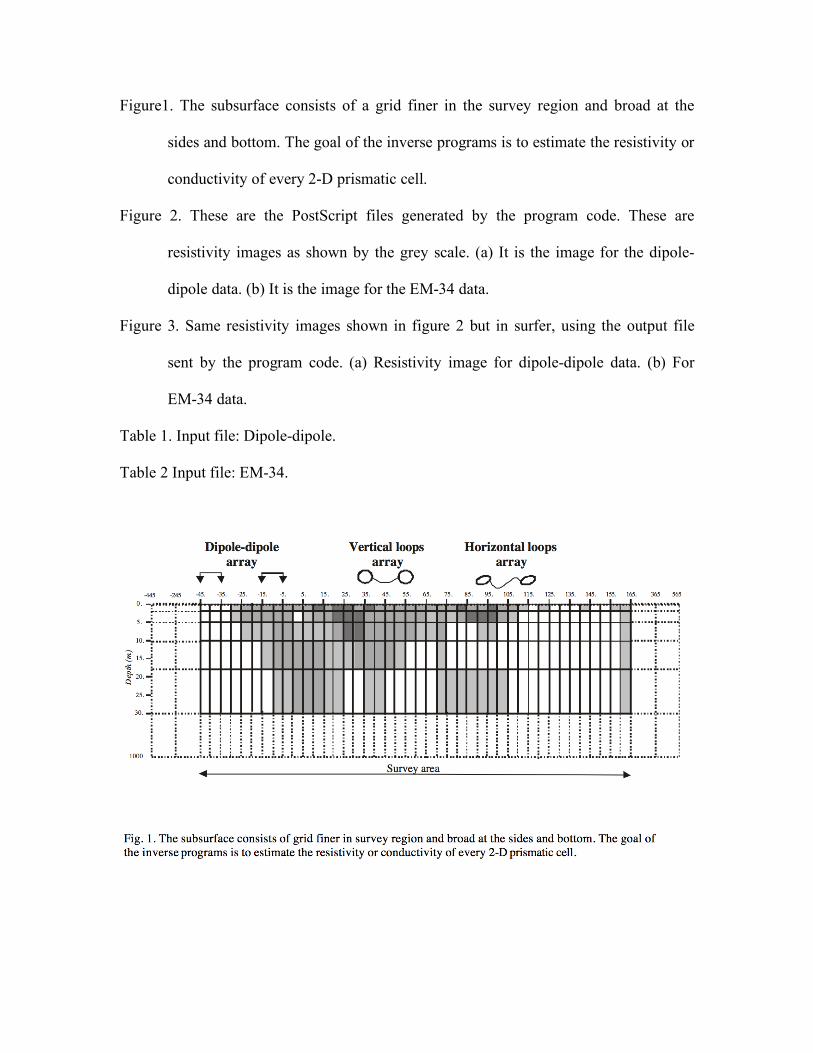
Figure1. The subsurface consists of a grid finer in the survey region and broad at the

sides and bottom. The goal of the inverse programs is to estimate the resistivity or

conductivity of every 2-D prismatic cell.

Figure 2. These are the PostScript files generated by the program code. These are

resistivity images as shown by the grey scale. (a) It is the image for the dipole-

dipole data. (b) It is the image for the EM-34 data.

Figure 3. Same resistivity images shown in figure 2 but in surfer, using the output file

sent by the program code. (a) Resistivity image for dipole-dipole data. (b) For

EM-34 data.

Table 1. Input file: Dipole-dipole.

Table 2 Input file: EM-34.

TABLE 1: DC RESISTIVITY 2D INVERSION SAMPLE FILE

TABLE 2: EM-LIN 2D INVERSION SAMPLE FILE