Intuitive Guide to Fourier...

Intuitive Guide to Fourier Analysis

Charan Langton

Victor Levin

Much of this book relies on math developed by important persons in the field over the last 200 years. When known or possible, the authors have given the credit due. We relied on many books and articles and consulted many articles on the internet and often many of these provided no name for credits. In this case, we are grateful to all who make the knowl-edge available free for all on the internet.

The publisher offers discounts on this book when ordered in quantity for bulk purchase or special sales. We can also make available on special or electronic version applicable to your business goals, such as training, marketing and branding issues. For more information, please contact us.

[email protected]

Website for this book: complextoreal.com/fftbook

Copyright 2016 Charan Langton and Victor LevinISBN- 13: 978-0-913063-26-2

All Rights reserved Printed in the United States of America. This publication is protected by copyright and permission must be obtained from the Publisher prior to prohibited repro-duction, storate in a retrieval system, recording. For information regarding permissions, please contact the publisher.

1 | Trigonometric Representation ofContinuous-time Periodic Signals

Jean-Baptiste Joseph Fourier1768 – 1830

Jean-Baptiste Joseph Fourier was a French mathematician and physicist. He ws appointedto the École Normale Supérieure, and subsequently succeeded Joseph-Louis Lagrange at the ÉcolePolytechnique. He is best known for developing the Fourier series and its applications to problemsof heat transfer and vibrations. The Fourier transform and Fourier’s Law are also named in hishonor. Fourier also did very important work in in the field of astronautics, as well as discoveringthe greenhouse effect for which he is not so well know. – From Wikipedia

What is Fourier analysisWhen sunlight hits rain-soaked air, an interesting phenomena happens. Water drops

take the ostensibly pure white light and split it into multiple colors. The mathematical de-scription of this process, the subject of this book, was first tackled by Newton approximately400 years ago. However, even though Newton was able to show that white light is in factcomposed of other colors, he was unable to make the jump to the idea that light can be de-scribed as waves. He called the component colors of white light “specter” or ghosts, from

1

CHAPTER 1. TRIGONOMETRIC REPRESENTATION

which we get the word spectrum. It took the development of trigonometric series and therecognition that light can be thought of as a composite wave before Fourier could apply theseideas to the problem of heat transfer. Although the concept of harmonic trigonometric seriesalready existed by the time he worked on the heat transfer problem, Fourier’s contributionis considered so important that the whole field of trigonometric waveform analysis and syn-thesis now bears his name, Fourier analysis.

Fourier developed the following partial differential equation called the Diffusion equa-tion to describe heat transfer through solids and other medium. Here v is a measure of heatand K , a heat diffusion constant of the material.

∂ v∂ t= K

∂ 2v∂ x2

(1.1)

Fourier observed that the most general solution to this equation was given as a linear sum-mation of sinusoids, i.e. sine and cosine waves of the form:

s(x) =∞∑

k=0

�

ak sin kx + bk cos kx�

(1.2)

This equation led Fourier to conclude that an arbitrary wave can be represented as asum of an infinite number of weighted sinusoids, i.e. sine and cosine waves. This trigono-metric summation is now known as the Fourier series. This book is all about this simple butimportant idea.

Fourier analysis is applicable to a wide variety of disciplines and not just signal pro-cessing, where it is now an essential tool. Fourier analysis is also used in image processing,geothermal and seismic studies, stochastic biological processes, quantum mechanics, acous-tics and even finance.

The Fourier analysis of waves or signals is similar to the concept of compound analysisin chemistry. Instead of atoms coming together to form a myriad of compounds, in signalprocessing sinusoids can be thought of as doing the same thing. A particular set of thesesinusoids is called the fundamental set. Just as a compound may consist of two units of oneelement and four units of another, an arbitrary wave can consist of two units of one funda-mental wave and four units of another. Hence we can create a particular wave by puttingtogether the fundamental waves. This process is called the Synthesis. Conversely, the pro-cess of decomposing an arbitrary wave is termed the Analysis. These two complementary,linear processes fall under the name of Fourier analysis and its analog, the Fourier trans-form.

2


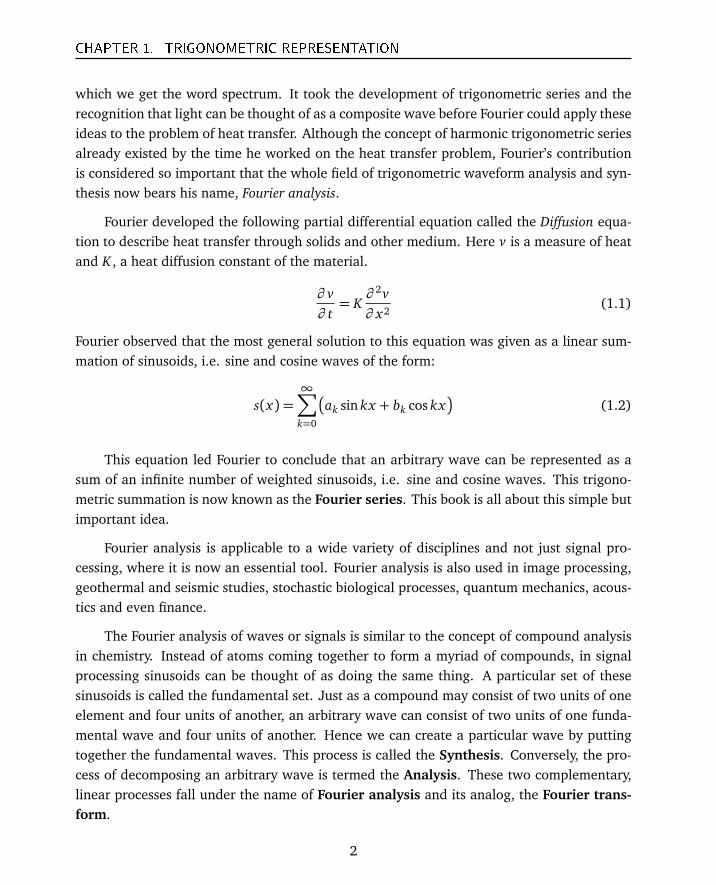
(a) Fourier Analysis (b) Fourier Synthesis

Figure 1.1: Fourier analysis is used to understand composite waves. (a) Analysis: breaking a givensignal into sine and cosine components and (b) Synthesis: adding certain sine and cosines to create a

desired signal.

Possibly it was the solution of Eq. (1.1) that led Fourier to notice that summation ofharmonic sine and cosine waves leads to some interesting looking periodic waves. From thishe posited that, conversely it is also possible to create any periodic signal by the summationof a particular set of harmonic sinusoids. This may not seem like a big thing now but it was arevolutionary insight at the time. Fourier’s discovery was met with incredulity at first. Manyof his contemporaries did not accept, and rightfully so, that his ideas did not apply to allsignals. After some years of work by Fourier as well as other famous mathematicians of theage, his theorem was upheld, albeit not under all conditions and not for all types of signals.Subsequent development led to the Fourier transform, the extension of Fourier’s original ideato non-periodic signals. But this computationally-demanding concept languished for over100 years, until the development of the Fast Fourier Transform (FFT), by J.W. Cooley andJohn Tukey in 1965. The FFT, an algorithmic technique, made the computation of Fourierseries simpler and quicker and finally allowed Fourier analysis to be recognized and usedwidely. It is now the premier tool of analysis in many fields.

Frequency and time domain views of a signal

Take the wave in Fig. 1.2. One would be hard pressed to guess its equation. Yet it isjust a sum of three waves shown in Fig. 1.3(a), 1.3(b) and 1.3(c) of differing frequenciesand amplitudes.

So although we know that the wave of Fig. 1.2 is created from the sum of three regularlooking sinusoids of Fig. 1.3, how could we determine this, if we did not already know theanswer?

3


0 0.5 1 1.5 2 2.5 3−4

−2

0

2

4

Time

Amplitude

Figure 1.2: An arbitrary periodic wave. We would like to know its equation, but how? Fourier analysisdoes not give us the actual equation but allows us to recreate it with a fair amount of accuracy using

simple sinusoids.

0 1 2 3−2

0

2

Amplitude

Time, t

0 1 2 3−2

0

2

0 1 2 3−2

0

2(a) Wave 1 (b) Wave 2 (c) Wave 3

Time, t Time, t

Figure 1.3: The components of the arbitrary wave of figure 1.2.

Spectrum of a signal

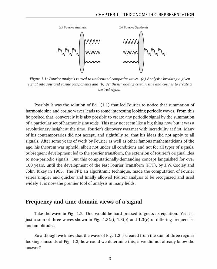
Let’s look at Fig. 1.4 showing a wave in three dimensions. When we see a signal, weare looking at it in what is called, the Time Domain. What we are actually observing is acomponent-summed signal. Its components may be several single-frequency waves, which weare unable to see. In this three dimensional view, when we look at the signal from the side,each component appears apart on the frequency axis. We see the constituent frequencies(also called components) in this view. From this view, we see only a single vertical line ateach of the discrete frequencies. This side view of the signal is called the Frequency Domain.Another name for this view is the Signal Spectrum.

The spectrum is a way to quantify the component frequencies. The spectrum of thesignal of Fig. 1.2 is composed of just three frequencies and can be drawn as in Fig. 1.5(a).This is called a one-sided amplitude spectrum. The x-axis in Fig. 1.5(a) represents the fre-quencies of the signal and, the y-axis is the amplitude of those frequencies. In (a), we seethe amplitude spectrum with amplitude of each frequency and in (b) we see the power spec-trum, a more typical representation. For power spectrum, we plot instead of amplitude, thequantity amplitude-squared (which is equal to the instantaneous power), commonly shownin Decibels (dBs).

The graphical representation such as the one shown in Fig. 1.5 is a unique signature ofthe signal at a particular time. Most signals we work with are not such deterministic sums

4


Time

3f

2f

1f

Harmonic

componen

ts

Amplitude

+

+

=

1f

2f

3f

Signal we see

Frequen

cy d

omai

n

1A

2A

3A

Time domain

Figure 1.4: Looking at a composite wave from time and frequency perspectives gives a different view ofthe same signal.

0 1 2 3 40

1

2

3

Am

pli

tud

e

Frequency, Hz

0 1 2 3 4

0

-6

6

Pow

er,

dB

Frequency, Hz

(a) Amplitude spectrum (b) Power spectrum

Amplitude of f1

Power in f1

Figure 1.5: The frequency view of the arbitrary wave of Fig. 1.2. (a) Shows the amplitude and (b)shows the power in dBs.

of sinusoids, so a spectrum is a distinctive and variable quality of a signal. It is not a staticthing but changes as the signal changes. Signals have distinctive spectrum and we can tell alot about a signal by looking only at its spectrum. The signals for which Fourier analysis isconsidered valid have stable spectrum that do not change much over time. This property isgenerally called textbfStationarity.

Fundamental waves and their harmonics

The basic building blocks of Fourier analysis are a set of harmonic sinusoids, called thebasis set. A basis set is our tinker-toy from which we can construct a variety of waves. Theset contains an infinite number of sinusoids of differing frequencies related in a special waythat we call harmonic.

We see a sinusoid of an arbitrary frequency in the first row of Fig. 1.6. Let’s call thisarbitrary frequency the fundamental frequency. We specify some waves based on this funda-

5


mental wave called the Harmonics. Each harmonic frequency is an integer multiple of thefrequency of the fundamental. We see in this figure that the second wave has half the wave-length and twice the frequency of the first one and so on. Each k-th wave has a wavelengthof T0/k and a frequency of k f0 with k being consecutive integers greater than 1. All suchwaves for k > 1 are called harmonics of the fundamental. The fundamental frequency is ofcourse arbitrary, it can be anything, but its harmonics are strictly integer multiples of it.

Fundamental

1st harmonic

2nd harmonic

0T

0

2

T

0

3

T

0f

02 f

03 f

Figure 1.6: The fundamental and its harmonic.

Let’s start with the expression of a complex sinusoid, a sine and a cosine of a certainfrequency:

s(t) = sin(2π f0 t)

c(t) = cos(2π f0 t)

Here f0 is an arbitrary frequency (measured in cycles/second or Hz). We will call this fre-quency the fundamental. The basic period T , of this sinusoid is inverse of the frequency.Note that if a sinusoid is periodic with period T , then it is also periodic with period 2T ,3T , etc. for integer multiples of the basic period. From this we get the definition of har-monic waves. A set of waves are harmonic if their frequency is an integer multiple of thefundamental wave’s frequency. We can write this as a set.

s(t) = sin(2π fk t)c(t) = cos(2π fk t)

(1.3)

Here we have introduced an index k such that each harmonic frequency is equal to k timesthe fundamental frequency with k any arbitrary integer.

fk = k f0 for k = 0, 1,2, . . . ,∞ (1.4)

In Fourier series formulation, the index k spans all positive integers to infinity, includingzero. Let’s rewrite the definition of the harmonics allowing the phase and the amplitude to

6


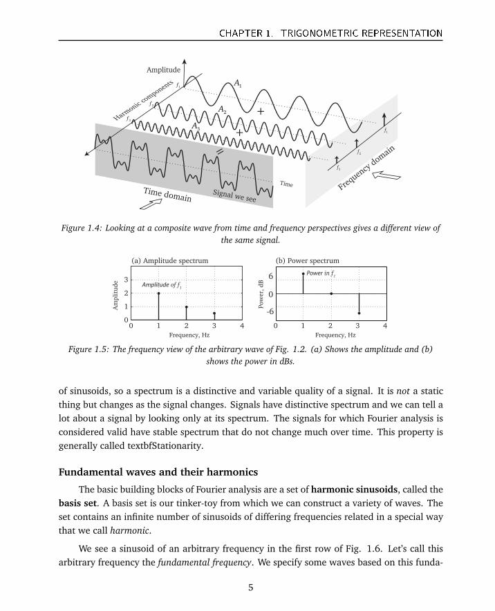
vary. We give each harmonic a unique amplitude and phase, hence we rewrite the harmonicsignals as:

sk(t) = Ak sin(2πk f0 t +φk)

ck(t) = Bk cos(2πk f0 t +φk)(1.5)

The wave ck(t) is a cosine wave of k-th harmonic frequency or k f0, its amplitude being Ak

and the phase in radians being φk. The signal sk(t) is a sine wave with similarly uniqueamplitude and phase for the same harmonic frequency, k f0. Now although the frequenciesare still related by multiples of k, we are allowing the amplitude and the phase of eachharmonic to be different. Such waves are still harmonic.

What is amplitude? This is value of the wave’s height at any particular time. For signals,it is often measured in volts. It can be positive or negative.

What is phase? A general sinusoid is defined by x(t) = A sin(ω0 t +φ). The term φ,a constant, is phase of the wave. We can think of it as the place the wave was at time, t =0. A sine wave is defined by setting it as φ = 0 radians. Cosine is defined by setting it toπ/2 at t = 0. Think of phase as a type of delay or maybe even as a starting point. Once set,phase does not change for linear signals. Here we assume that phase and frequency are nota function of time.

−1 −0.5 0 0.5 1

−2

0

2

(a) Sine wave of freq = 1 Hz

−1 −0.5 0 0.5 1−2

0

2(b) Sine wave of freq = 2 Hz

−1 −0.5 0 0.5 1−2

0

2(c) Sine wave of freq = 3 Hz

−1 −0.5 0 0.5 1−2

0

2(d) Cosine wave of freq = 1 Hz

−1 −0.5 0 0.5 1−2

0

2(e) Cosine wave of freq = 2 Hz

−1 −0.5 0 0.5 1−2

0

2(f) Cosine wave of freq = 3 Hz

Am

pli

tud

eA

mpli

tud

eA

mpli

tud

e

Sine waves Cosine waves

Time, t Time, t

Figure 1.7: The fundamental of f0 = 1 Hz and its two cosine and sine harmonics. All sines start at 0and all cosines at peak amplitude.

7


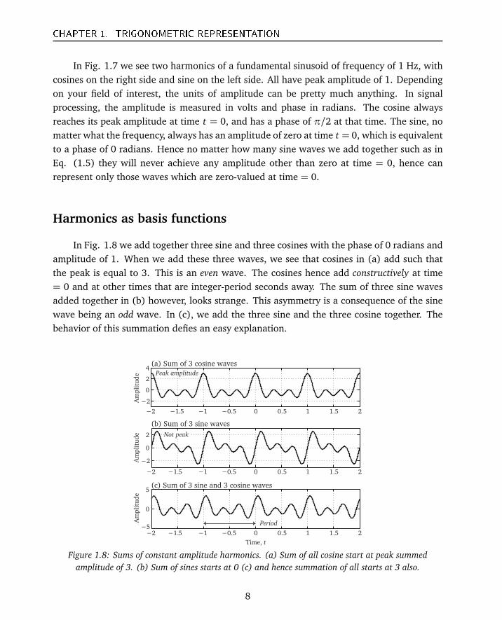
In Fig. 1.7 we see two harmonics of a fundamental sinusoid of frequency of 1 Hz, withcosines on the right side and sine on the left side. All have peak amplitude of 1. Dependingon your field of interest, the units of amplitude can be pretty much anything. In signalprocessing, the amplitude is measured in volts and phase in radians. The cosine alwaysreaches its peak amplitude at time t = 0, and has a phase of π/2 at that time. The sine, nomatter what the frequency, always has an amplitude of zero at time t = 0, which is equivalentto a phase of 0 radians. Hence no matter how many sine waves we add together such as inEq. (1.5) they will never achieve any amplitude other than zero at time = 0, hence canrepresent only those waves which are zero-valued at time = 0.

Harmonics as basis functions

In Fig. 1.8 we add together three sine and three cosines with the phase of 0 radians andamplitude of 1. When we add these three waves, we see that cosines in (a) add such thatthe peak is equal to 3. This is an even wave. The cosines hence add constructively at time= 0 and at other times that are integer-period seconds away. The sum of three sine wavesadded together in (b) however, looks strange. This asymmetry is a consequence of the sinewave being an odd wave. In (c), we add the three sine and the three cosine together. Thebehavior of this summation defies an easy explanation.

−2 −1.5 −1 −0.5 0 0.5 1 1.5 2

−2

0

2

(b) Sum of 3 sine waves

−2 −1.5 −1 −0.5 0 0.5 1 1.5 2

−2

0

2

4(a) Sum of 3 cosine waves

−2 −1.5 −1 −0.5 0 0.5 1 1.5 2−5

0

5(c) Sum of 3 sine and 3 cosine waves

Am

pli

tud

eA

mpli

tud

eA

mpli

tud

e

Peak amplitudePeak amplitudePeak amplitude

Period

Time, t

Not peak

Figure 1.8: Sums of constant amplitude harmonics. (a) Sum of all cosine start at peak summedamplitude of 3. (b) Sum of sines starts at 0 (c) and hence summation of all starts at 3 also.

8


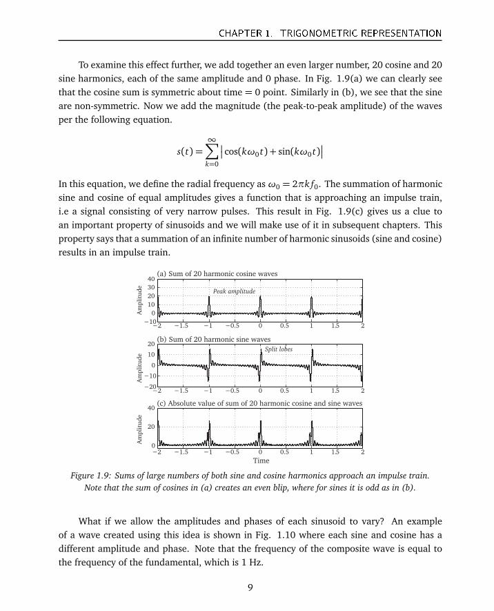
To examine this effect further, we add together an even larger number, 20 cosine and 20sine harmonics, each of the same amplitude and 0 phase. In Fig. 1.9(a) we can clearly seethat the cosine sum is symmetric about time = 0 point. Similarly in (b), we see that the sineare non-symmetric. Now we add the magnitude (the peak-to-peak amplitude) of the wavesper the following equation.

s(t) =∞∑

k=0

�

� cos(kω0 t) + sin(kω0 t)�

�

In this equation, we define the radial frequency asω0 = 2πk f0. The summation of harmonicsine and cosine of equal amplitudes gives a function that is approaching an impulse train,i.e a signal consisting of very narrow pulses. This result in Fig. 1.9(c) gives us a clue toan important property of sinusoids and we will make use of it in subsequent chapters. Thisproperty says that a summation of an infinite number of harmonic sinusoids (sine and cosine)results in an impulse train.

−2 −1.5 −1 −0.5 0 0.5 1 1.5 2−10

0

10

20

30

40(a) Sum of 20 harmonic cosine waves

−2 −1.5 −1 −0.5 0 0.5 1 1.5 2−20

−10

0

10

20(b) Sum of 20 harmonic sine waves

−2 −1.5 −1 −0.5 0 0.5 1 1.5 20

20

40(c) Absolute value of sum of 20 harmonic cosine and sine waves

Am

pli

tud

eA

mpli

tud

eA

mpli

tud

e

Time

Peak amplitude

Split lobes

Figure 1.9: Sums of large numbers of both sine and cosine harmonics approach an impulse train.Note that the sum of cosines in (a) creates an even blip, where for sines it is odd as in (b).

What if we allow the amplitudes and phases of each sinusoid to vary? An exampleof a wave created using this idea is shown in Fig. 1.10 where each sine and cosine has adifferent amplitude and phase. Note that the frequency of the composite wave is equal tothe frequency of the fundamental, which is 1 Hz.

9


s(t) = 0.1 cos(2πt − 0.5) + 0.3 cos(4πt)− 0.4cos(6πt − 0.1)

− 0.5 sin(2πt + 0.1)− 0.8 sin(4πt − 0.3) + 0.67 sin(6πt + .19) (1.6)

The most important thing to note is that by adding any number of harmonics, and allow-ing the amplitudes and phase of each to vary, we can create or mimic many other waves. InFig. 1.10, we have an example of just one such “interesting” looking wave created by usingonly three different sinusoids of distinctly different amplitudes and phases. This is exactlythe idea behind Fourier synthesis and analysis.

−2 −1.5 −1 −0.5 0 0.5 1 1.5 2−2

0

2

Am

pli

tud

e

Time, t

Period

Figure 1.10: A wave composed of arbitrary amplitude harmonics of Eq. (1.6) begins to look“interesting”.

Even and oddness of sinusoids

Sinusoids have a lot of interesting properties. There are a few that are important inFourier analysis. One important property of harmonic sine and cosine waves is the symmetryor the oddness of the wave. All sine waves are considered odd functions because they obeythe following definition of an odd function.

f (x) = − f (−x) (1.7)

If you look at a sine wave, you see that it starts with an amplitude of 0 at time = 0. If wewere to flip it about the y-axis, the images would not overlap. But if one of the sides was firstflipped about the x-axis, then they do overlap. That is a description of oddness of signals.It requires two flips for values to coincide, as we can see from the two negative signs in Eq.(1.7).

The cosine waves on the other hand are called even functions by a similar definition.The two sides of a cosine wave, if flipped about the y-axis, would overlap, hence there isonly one negative in the equation below for even symmetry.

f (x) = f (−x) (1.8)

10


By the superposition principle, if multiple odd waves are summed together, the resultingwave will remain odd. If multiple even waves are summed, then the resulting wave willremain even. A mixture will have no symmetry. This becomes important when synthesizing,which is the process of putting some waves together to make a desired wave. If a wave tobe synthesized is purely odd, or an even function, then it will only contain sine, or cosine,depending on its symmetry.

Making waves

Square waves

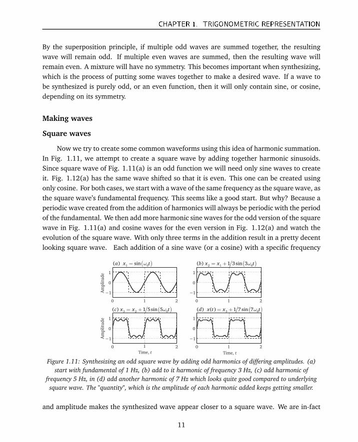
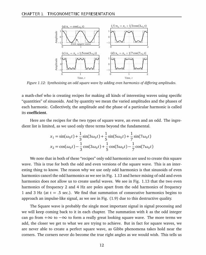
Now we try to create some common waveforms using this idea of harmonic summation.In Fig. 1.11, we attempt to create a square wave by adding together harmonic sinusoids.Since square wave of Fig. 1.11(a) is an odd function we will need only sine waves to createit. Fig. 1.12(a) has the same wave shifted so that it is even. This one can be created usingonly cosine. For both cases, we start with a wave of the same frequency as the square wave, asthe square wave’s fundamental frequency. This seems like a good start. But why? Because aperiodic wave created from the addition of harmonics will always be periodic with the periodof the fundamental. We then add more harmonic sine waves for the odd version of the squarewave in Fig. 1.11(a) and cosine waves for the even version in Fig. 1.12(a) and watch theevolution of the square wave. With only three terms in the addition result in a pretty decentlooking square wave. Each addition of a sine wave (or a cosine) with a specific frequency

0 1 2

−1

0

1

0 1 2

−1

0

1

0 1 2

−1

0

1

0 1 2

−1

0

1

( )2 1 0( ) 1 3sin 3b x x tω= +( )1 0( ) sina x tω=

( )3 2 0( ) 1 5sin 5c x x tω= + ( )3 0( ) ( ) 1 7sin 7d x t x tω= +

Amplitude

Time, t

Amplitude

Time, t

Figure 1.11: Synthesizing an odd square wave by adding odd harmonics of differing amplitudes. (a)start with fundamental of 1 Hz, (b) add to it harmonic of frequency 3 Hz, (c) add harmonic of

frequency 5 Hz, in (d) add another harmonic of 7 Hz which looks quite good compared to underlyingsquare wave. The "quantity", which is the amplitude of each harmonic added keeps getting smaller.

and amplitude makes the synthesized wave appear closer to a square wave. We are in-fact

11


0 1 2

−1

0

1

0 1 2

−1

0

1

0 1 2

−1

0

1

0 1 2

−1

0

1

1 0( ) x cos( t)a ω= 2 1 0( ) x 1 3cos(3 t)f x ω= +

3 2 0(c) x 1 5cos(5 t)x ω= + 4 3 0(d) x 1 7cos(7 t)x ω= +

Even square wave

Amplitude

Amplitude

Time, t Time, t

Figure 1.12: Synthesizing an odd square wave by adding even harmonics of differing amplitudes.

a math-chef who is creating recipes for making all kinds of interesting waves using specific“quantities” of sinusoids. And by quantity we mean the varied amplitudes and the phases ofeach harmonic. Collectively, the amplitude and the phase of a particular harmonic is calledits coefficient.

Here are the recipes for the two types of square wave, an even and an odd. The ingre-dient list is limited, as we used only three terms beyond the fundamental.

x1 = sin(ω0 t) +13

sin(3ω0 t) +15

sin(5ω0 t) +17

sin(7ω0 t)

x2 = cos(ω0 t)−13

cos(3ω0 t) +15

cos(5ω0 t)−17

cos(7ω0 t)

We note that in both of these “recipes” only odd harmonics are used to create this squarewave. This is true for both the odd and even versions of the square wave. This is an inter-esting thing to know. The reason why we use only odd harmonics is that sinusoids of evenharmonics cancel the odd harmonics as we see in Fig. 1.13 and hence mixing of odd and evenharmonics does not allow us to create useful waves. We see in Fig. 1.13 that the two evenharmonics of frequency 2 and 4 Hz are poles apart from the odd harmonics of frequency1 and 3 Hz (at t = .5 sec.). We find that summation of consecutive harmonics begins toapproach an impulse-like signal, as we see in Fig. (1.9) due to this destructive quality.

The Square wave is probably the single most important signal in signal processing andwe will keep coming back to it in each chapter. The summation with k as the odd integercan go from +∞ to −∞ to form a really great looking square wave. The more terms weadd, the closer we get to what we are trying to achieve. But in fact for square waves, weare never able to create a perfect square wave, as Gibbs phenomena takes hold near thecorners. The corners never do become the true right angles as we would wish. This tells us

12


0.2 0.4 0.6 0.8 1−1

0

1

1,3

2,41

2

3

4

Amplitude

Time, t

1 Hz

2 Hz

3 Hz

4 Hz

Figure 1.13: Even order harmonics are destructive and hence are not used in combination with odds tocreate most communications signals such as square waves.

that this form of harmonic representation, despite our best efforts, may not result in a perfectreconstruction for every signal. A square wave is one of those signals.

Gibbs phenomenon

In Fig. 1.14, we see that even as k, the number of terms in the square wave summationis increased, the oscillation at the corner points never goes away. This behavior called theGibbs phenomenon is a clear demonstration of the fact that Fourier representation can notmimic all periodic waves. Hence waveforms that have hard discontinuities in amplitude, areavoided in signal processing. Instead of true square waves, we use shaped waves with gentlecorners and curves which are easier to represent with sinusoids.

−2 0 2

0

1

2

−2 0 2

0

1

2

−2 0 2

0

1

2

−2 0 2

0

1

2

Am

pli

tud

eA

mpli

tud

e

(a) K = 5 (b) K = 11

(c) K = 30 (d) K = 70

Time, t Time, t

Figure 1.14: Gibbs phenomena does not allow for a perfect Fourier representation of a square wave.

Creating a sawtooth wave

Let’s look at one more special signal, a sawtooth wave. The sawtooth wave is an oddfunction hence composed only of sine waves. We give its equation as

sawtooth(t) =2π

∞∑

k=1

(−1)k+1 sin(2πk f0 t)k

(1.9)

13


0 1 2 3−0.5

0

0.5

0 1 2 3−0.5

0

0.5

0 1 2 3−0.5

0

0.5

0 1 2 3−0.5

0

0.5

(a) K = 1 (b) K = 5

(c) K = 11 (d) K = 20Amplitude

Amplitude

Time, t Time, t

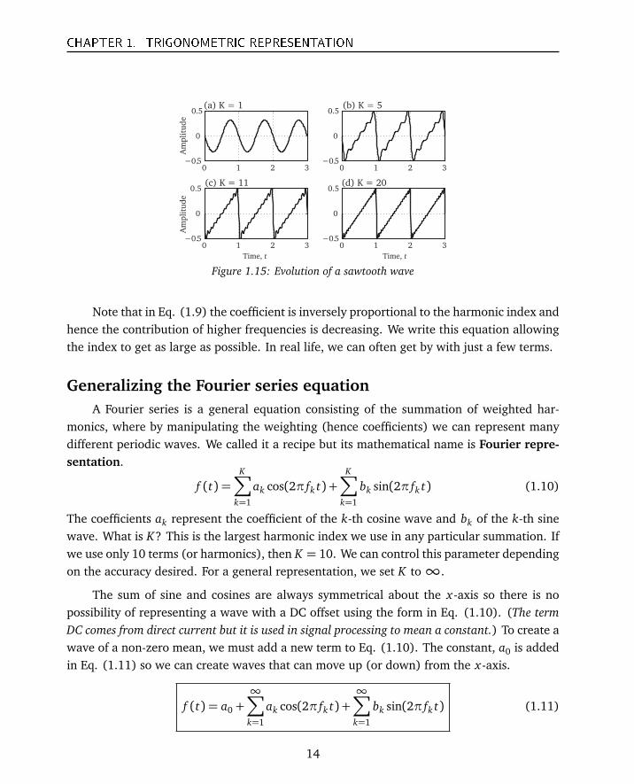
Figure 1.15: Evolution of a sawtooth wave

Note that in Eq. (1.9) the coefficient is inversely proportional to the harmonic index andhence the contribution of higher frequencies is decreasing. We write this equation allowingthe index to get as large as possible. In real life, we can often get by with just a few terms.

Generalizing the Fourier series equationA Fourier series is a general equation consisting of the summation of weighted har-

monics, where by manipulating the weighting (hence coefficients) we can represent manydifferent periodic waves. We called it a recipe but its mathematical name is Fourier repre-sentation.

f (t) =K∑

k=1

ak cos(2π fk t) +K∑

k=1

bk sin(2π fk t) (1.10)

The coefficients ak represent the coefficient of the k-th cosine wave and bk of the k-th sinewave. What is K? This is the largest harmonic index we use in any particular summation. Ifwe use only 10 terms (or harmonics), then K = 10. We can control this parameter dependingon the accuracy desired. For a general representation, we set K to∞.

The sum of sine and cosines are always symmetrical about the x-axis so there is nopossibility of representing a wave with a DC offset using the form in Eq. (1.10). (The termDC comes from direct current but it is used in signal processing to mean a constant.) To create awave of a non-zero mean, we must add a new term to Eq. (1.10). The constant, a0 is addedin Eq. (1.11) so we can create waves that can move up (or down) from the x-axis.

f (t) = a0 +∞∑

k=1

ak cos(2π fk t) +∞∑

k=1

bk sin(2π fk t) (1.11)

14


Eq. (1.11) is called the Fourier series equation. The coefficients a0, ak, bk are called theFourier Series Coefficients (FSC) . The process of Fourier analysis consists of computingthese three types of coefficients, given an arbitrary periodic wave, f (t).

Multiple ways of writing the Fourier series equation

We find several different forms of the Fourier series equation in literature, and thatmakes understanding this equation confusing. One common representation is by using theradial frequency ωk = 2π fk to make the equation simpler to type. We can write this form ofFourier series as

f (t) = a0 +∞∑

k=1

ak cos(ωk t) +∞∑

k=1

bk sin(ωk t) (1.12)

Now we define T0 the period of the fundamental frequency.

T0 =1f0

Then the period of the k-th harmonic becomes T0/k and its frequency, fk = k/T0. We canalternately write the Fourier series equation by adopting this form of the frequency in Eq.(1.13).

f (t) = a0 +∞∑

k=1

ak cos�

2πkT0

t�

+∞∑

k=1

bk sin�

2πkT0

t�

(1.13)

This is an another way to write-out the Fourier series representation. We specifically addedthe DC term, now we look at a way to get rid of it. We can shorten the Fourier series equationby starting at zero frequency, hence index k starts at 0 instead of at 1. Now the DC termdisappears as it is included as the zero frequency coefficient obtained by setting the indexk = 0. The DC term is now included as the 0-th coefficient. Now we have this new form withthe DC term gone.

f (t) =∞∑

k=0

ak cos(2π fk t) + bk sin(2π fk t) (1.14)

We can simplify even more. We can get rid of the sine terms in Eq. (1.12) altogether. Weknow that sine and cosine are really the same thing, one is just the shifted version of theother. The representation in Eq. (1.12) can be written solely with cosine by shifting eachsine wave by π. This way sine becomes a cosine and we only need cosine in the Fourier

15


series, making it more concise.

f (t) = a0 +∞∑

k=1

ck cos(ωk t +φk) (1.15)

Each harmonic, whether a sine or a cosine can be thought of as really a cosine of somephase. The sine is actually a cosine with shifted phase (or start point) and can be writtenas sin(kω0 t) = cos(kω0 t + φ). In expanded form Eq. (1.15) will look like this. Now notonly are the amplitudes variable but so are the phases and the whole expression uses onlythe cosine waves.

f (t) = c0 + c1 cos(ω1 t ±φ1) + c2 cos(ω2 t ±φ2) + c3 cos(ω3 t ±φ3) + . . .

Fourier series in the complex form

In its most important representation, the complex representation, the Fourier series iswritten as

f (t) =∞∑

k=−∞Cke j2π k

T0t (1.16)

Here we introduce a new term, called the complex exponential. It even looks complex,

e j2π kT0

t . It can represent both a sine and a cosine by change of the sign of the exponent. Inthe next chapter we will discuss this function in detail. The expanded form of the Fourierseries in terms of the complex exponential looks like this.

f (t) = C0 + C1e j2π 1T0

t + C2e j2π 2T0

t + C3e j2π 3T0

t + . . .

This form says that we can create a periodic function by summing together complex expo-nentials. Although the complex form of the Fourier series is scary looking, it is the most usedform. In next chapter, we will look at how it is derived and why we use it in Fourier analysis.

All these different representations of the Fourier series are identical and mean exactlythe same thing. They are all the many ways you see Fourier representation in books.

The Fourier Analysis

The process of adding together a bunch of sinusoids to create useful waves is called theSynthesis process. Synthesis of waveforms is of course interesting but what is really usefulis to take an arbitrary periodic signal and figure out its components. Sort of like trying to

16


figure out what the ingredients of a particular dish. By ingredients, we mean frequenciesin the signal that contain significant power or amplitudes. This is the main use of Fourieranalysis. It is called, not surprisingly, the Analysis part. What this involves is to make aguess of the fundamental frequency f0, and then computing the amplitudes (coefficients) ofa certain number of harmonics. It is no guarantee that the fundamental we choose will resultin finding all the main signal components exactly. But in most cases, we have a pretty goodidea of signal components a-priori. So the process works well enough.

The usefulness of the process can be seen in the equation of the sawtooth wave in Eq.(1.9). Fourier series allows us to create an estimate of the wave using a few or a lot of terms.Hence Fourier series represents an estimate of the true representation, which can have anynumber of terms.

The Fourier analysis process consists of finding the series coefficients. When we talkabout Fourier series coefficients (FSC), we are talking about the amplitudes of the sine andcosine harmonics, and nothing else. Once we decide on a fundamental frequency, a startingpoint for the analysis, we already know all the harmonic frequencies since they are integermultiples of the fundamental frequency. All we have to do now is to compute these Fouriercoefficients.

1. Coefficients of the cosine ak cos(2πk f0 t) with k = 1, 2,3, . . . ,∞.2. Coefficients of the sine bk sin(2πk f0 t) with k = 1,2, 3, . . . ,∞.3. The DC offset or the coefficient of the 0-th frequency, k = 0.

We will look at each of these three types of coefficients separately and see how to computethem.

Computing a0, the DC coefficient

We are given an arbitrary periodic signal, f (t) of period T. Fourier series says that thesignal f (t) is composed of a summation of K sinusoidal harmonics. Our task is to find thecoefficients of each of these harmonics starting with k = 0 to k = K .

f (t) = a0 +∞∑

k=1

ak cos(2π fk t) + bk sin(2π fk t) (1.17)

The constant a0 in the Fourier series equation represents the DC offset. If our target wavehas a nonzero DC component (if its average amplitude value is not zero), then we knowthat a0 6= 0. But before we compute it, let’s take a look at another useful property of sineand cosine waves. Both sine and cosine waves are symmetrical about the x-axis. When youintegrate a sine or a cosine wave over one period, you always get zero. The area above the

17


0 0.25 0.5 0.75 1−1

0

1

Amplitude

0 0.25 0.5 0.75 1−1

0

1

Amplitude

(a) One period of sine (b) One period of cosine

Time, t Time, t

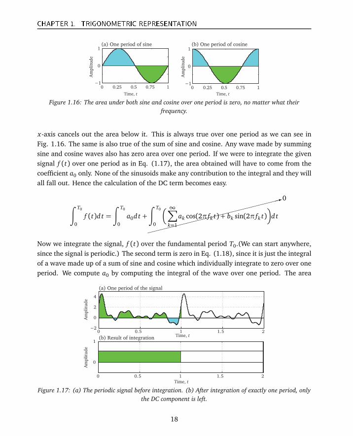
Figure 1.16: The area under both sine and cosine over one period is zero, no matter what theirfrequency.

x-axis cancels out the area below it. This is always true over one period as we can see inFig. 1.16. The same is also true of the sum of sine and cosine. Any wave made by summingsine and cosine waves also has zero area over one period. If we were to integrate the givensignal f (t) over one period as in Eq. (1.17), the area obtained will have to come from thecoefficient a0 only. None of the sinusoids make any contribution to the integral and they willall fall out. Hence the calculation of the DC term becomes easy.

∫ T0

0

f (t)d t =

∫ T0

0

a0d t +

��

��

��

��:0

∫ T0

0

� ∞∑

k=1

ak cos(2π fk t) + bk sin(2π fk t)�

d t

Now we integrate the signal, f (t) over the fundamental period T0.(We can start anywhere,since the signal is periodic.) The second term is zero in Eq. (1.18), since it is just the integralof a wave made up of a sum of sine and cosine which individually integrate to zero over oneperiod. We compute a0 by computing the integral of the wave over one period. The area

0 0.5 1 1.5 2

0

1

Am

pli

tud

e

(a) One period of the signal

0 0.5 1 1.5 2−2

0

2

4

Am

pli

tud

e

(b) Result of integrationTime, t

Time, t

Figure 1.17: (a) The periodic signal before integration. (b) After integration of exactly one period, onlythe DC component is left.

18


under one period of this wave is equal to∫ T0

0

f (t)d t =

∫ T0

0

a0d t

Integrating this simple equation, we get,∫ T0

0

f (t)d t = a0T0

We can now write a very easy equation for a0

a0 =1T0

∫ T0

0

f (t)d t (1.18)

Summary: To compute the DC coefficient, we integrate f (t) over one period. (What is thatperiod? It is the period of the fundamental.) The result of the integration is equal to the 0-thcoefficient.

Computing bk, the coefficients of sine waves

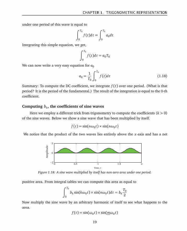
Here we employ a different trick from trigonometry to compute the coefficients (k > 0)of the sine waves. Below we show a sine wave that has been multiplied by itself.

f (t) = sin(nω0 t)× sin(nω0 t)

We notice that the product of the two waves lies entirely above the x-axis and has a net

0 0.5 1 1.5 2−2

0

2

Amplitude

Time, t

Figure 1.18: A sine wave multiplied by itself has non-zero area under one period.

positive area. From integral tables we can compute this area as equal to∫ T0

0

bk sin(kω0 t)× sin(nω0 t)d t = bkT0

2

Now multiply the sine wave by an arbitrary harmonic of itself to see what happens to thearea.

f (t) = sin(ω0 t)× sin(mω0 t)

19


0 0.5 1 1.5 2

−1

0

1

Amplitude

Time, t

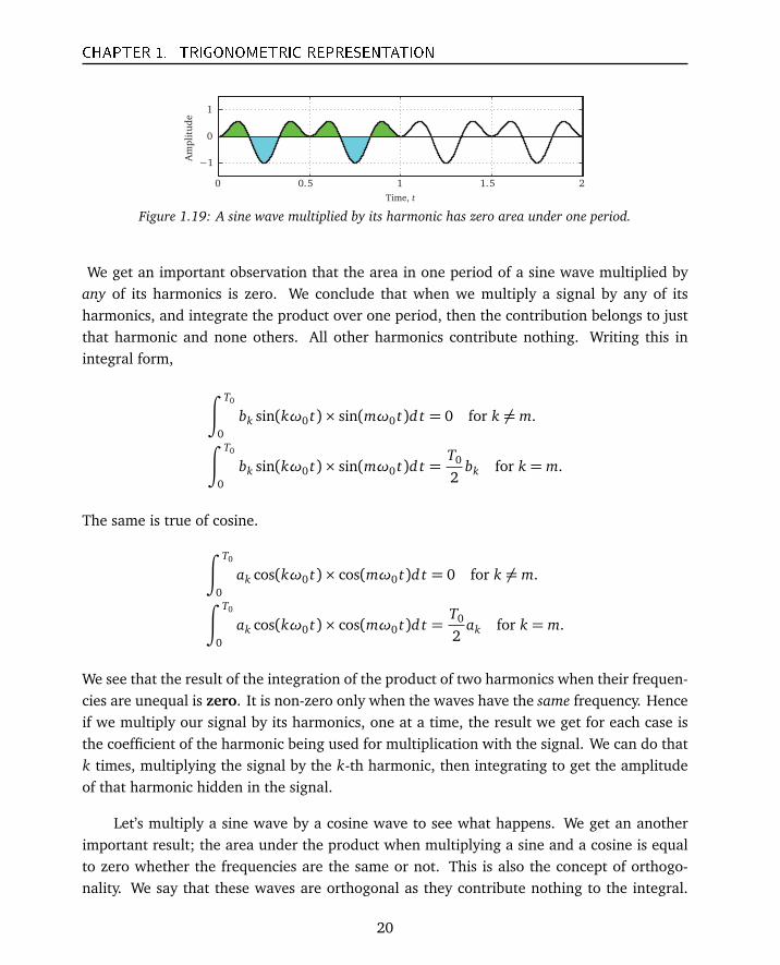
Figure 1.19: A sine wave multiplied by its harmonic has zero area under one period.

We get an important observation that the area in one period of a sine wave multiplied byany of its harmonics is zero. We conclude that when we multiply a signal by any of itsharmonics, and integrate the product over one period, then the contribution belongs to justthat harmonic and none others. All other harmonics contribute nothing. Writing this inintegral form,

∫ T0

0

bk sin(kω0 t)× sin(mω0 t)d t = 0 for k 6= m.

∫ T0

0

bk sin(kω0 t)× sin(mω0 t)d t =T0

2bk for k = m.

The same is true of cosine.

∫ T0

0

ak cos(kω0 t)× cos(mω0 t)d t = 0 for k 6= m.

∫ T0

0

ak cos(kω0 t)× cos(mω0 t)d t =T0

2ak for k = m.

We see that the result of the integration of the product of two harmonics when their frequen-cies are unequal is zero. It is non-zero only when the waves have the same frequency. Henceif we multiply our signal by its harmonics, one at a time, the result we get for each case isthe coefficient of the harmonic being used for multiplication with the signal. We can do thatk times, multiplying the signal by the k-th harmonic, then integrating to get the amplitudeof that harmonic hidden in the signal.

Let’s multiply a sine wave by a cosine wave to see what happens. We get an anotherimportant result; the area under the product when multiplying a sine and a cosine is equalto zero whether the frequencies are the same or not. This is also the concept of orthogo-nality. We say that these waves are orthogonal as they contribute nothing to the integral.

20


0 0.5 1 1.5 2

−1

0

1

Amplitude

Time, t

Figure 1.20: A sine wave multiplied by a cosine has total area of zero under one period.

Summarizing

∫ T0

0

bk sin(kω0 t)× sin(mω0 t)d t = 0 for n 6= m

∫ T0

0

bk sin(kω0 t)× sin(mω0 t)d t =T0

2bk for n= m

∫ T

0

bk cos(nω0 t)× sin(mω0 t)d t = 0 (1.19)

Another very satisfying interpretation of these properties is that sine and cosine wavesact as filtering signals. In essence they act as a narrow-band filter and ignore all frequenciesexcept the one of interest. This is the fundamental concept of a filter.

Here are the key results.

1. If you multiply a sine or a cosine wave by any of its harmonics, the area under theproduct is zero.

2. If you multiply a sine or a cosine of a particular frequency by itself, the area under theproduct is proportional to the Fourier coefficient of that frequency.

3. The area under a sine wave multiplied by a harmonic cosine is always zero. (Becausesine and cosine are orthogonal!)

We use this information to compute the bk coefficients. Successively multiply the targetsignal, f (t) by a sine wave of a specific harmonic and then integrate over one period as inequation below.

∫ T0

0

f (t) sin(kω0 t)d t =��

��

�:0∫ T0

0

a0 sin(kω0 t)d t +

∫ T0

0

bk sin(kω0 t) sin(kω0 t)d t

+��

��

��:

0∫ T0

0

ak cos(kω0 t) sin(kω0 t)d t (1.20)

21


We know that the integral of the first and the third term in Eq. (1.20) is zero since the firstterm is just the integral of a sine wave multiplied by a constant and the third term is of a sinewave multiplied by a cosine wave. This simplifies our equation considerably. We know thatthe integral of the second term is

∫ T0

0

bk sin(kω0 t) sin(kω0 t)d t =bkT0

2

From this we obtain bk as follows

bk =2T0

∫ T0

0

f (t) sin(kω0 t)d t (1.21)

The coefficient bk is hence computed by taking the target signal over one period, successivelymultiplying it with a sine wave of k-th harmonic frequency and then integrating. This givesthe coefficient for that particular harmonic. If we do this K times, we get K individual bk

coefficients.

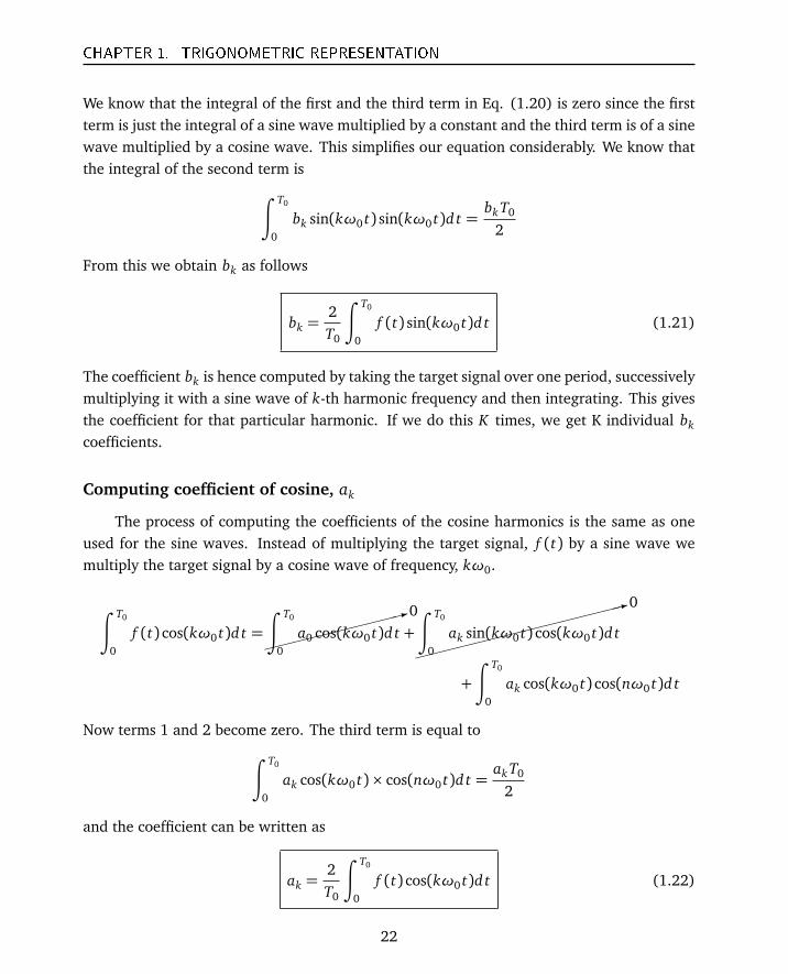
Computing coefficient of cosine, ak

The process of computing the coefficients of the cosine harmonics is the same as oneused for the sine waves. Instead of multiplying the target signal, f (t) by a sine wave wemultiply the target signal by a cosine wave of frequency, kω0.

∫ T0

0

f (t) cos(kω0 t)d t =��

��

��:0∫ T0

0

a0 cos(kω0 t)d t +��

��

��:

0∫ T0

0

ak sin(kω0 t) cos(kω0 t)d t

+

∫ T0

0

ak cos(kω0 t) cos(nω0 t)d t

Now terms 1 and 2 become zero. The third term is equal to

∫ T0

0

ak cos(kω0 t)× cos(nω0 t)d t =akT0

2

and the coefficient can be written as

ak =2T0

∫ T0

0

f (t) cos(kω0 t)d t (1.22)

22


So the process of finding the coefficients is multiplying the target signal with successivelylarger harmonic frequencies of a cosine wave and integrating the results. This is easy to doin software. The result obtained is the coefficient for that specific frequency of sine wave.We do the same thing for cosine coefficients. Conceptually the process of computing thecoefficients consists of filtering the target signal, one frequency at a time. In software whenwe compute the spectrum, this is exactly what we are doing hence a spectrum can be seenas tiny little filters that pull out the quantity of that harmonic in the signal. And by quantitywe mean the amplitude of the harmonic.

Example 1.1. Find the Fourier series coefficients for the function:

f (t) =�

cos(2πt)�3

From Fig. 1.21 we can immediately spot two pieces of information. The first is that the periodthe wave is 1 second long (its frequency is 1 Hz), and second, that the symmetry of the signalis even. Because it is an even signal, we know that it only contains cosine components. (Butof course that makes sense as the function is cosine cubed.)

First we calculate the a0 coefficient to determine the DC offset.

a0 =

∫ 1

0

�

cos(2πt)�3

d t = 0

This result agrees with the graph. There is symmetry about the x-axis meaning there is noDC offset. Now using Eq. (1.22) we can determine the ak coefficients (of cosine) startingwith the fundamental harmonic. The fundamental frequency f0 is 1 Hz.

a1 = 2

∫ 1

0

�

cos(2πt)�3

cos(1× 2πt)d t = 0.75

Here is the plot of only the a1 coefficient cosine wave. It is clear that one coefficient is not

−1.5 −1 −0.5 0 0.5 1 1.5

−1

0

1

Am

pli

tud

e ( )3

cos(2 )tπ

cos(2 )tπ

Time, t

Figure 1.21:�

cos(2πt)�3

solid curve and its first order representation.

23


enough to fully represent the signal. We calculate a few more coefficients.

a2 = 2

∫ 1

0

�

cos(2πt)�3

cos(2× 2πt)d t = 0

a3 = 2

∫ 1

0

�

cos(2πt)�3

cos(3× 2πt)d t = 0.25

With a0 = 0, a1 = .75, a2 = 0, and a3 = 0.25 the series is given as

f (x) = .75cos(2πt) + .25cos(6πt)

Using trigonometric identities this can be proven to be equal to cos3(2πt). If we continue tocalculate more ak coefficients (for k > 3) we will see that they are all zero after a3. From thiswe can say that function cosine cubed is in fact made up of only two cosines of frequency 1and 3 Hz. In this case, Fourier series representation is an exact representation of the signal,but this is not always the case.

Example 1.2. Find the Fourier series coefficients for the function:

f (t) = sin2(2πt) + sin(2πt)

−1.5 −1 −0.5 0 0.5 1 1.5

0

1

2

Am

pli

tud

e

Time, t

Figure 1.22: sin2(2πt) + sin(2πt).

Using trigonometric identities we can rewrite the function as:

f (t) =12+ sin(2πt)−

12

cos(4πt)

From this we can expect to have a non-zero a0 coefficient for the DC offset, a a2 cosinecoefficient and a b1 sine coefficient. The values of these will match the coefficients of thesignals’ equation. The results of the integrals show that this is indeed the case. The Fourierrepresentation in this case is exact. This only happens if the original signal it composedonly of harmonic sinusoids. In real life, this situation is unlikely and hence our Fourier

24


representation is usually only an approximation.

a0 =

∫ 1

0

�

sin2(2πt) + sin(2πt)�

d t =12

a1 = 2

∫ 1

0

�

sin2(2πt) + sin(2πt)) cos(1 · 2πt)�

d t = 0

a2 = 2

∫ 1

0

�

sin2(2πt) + sin(2πt)) cos(2 · 2πt)�

d t = −12

b1 = 2

∫ 1

0

�

sin2(2πt) + sin(2πt)) sin(1 · 2πt)�

d t = 1

b2 = 2

∫ 1

0

�

sin2(2πt) + sin(2πt)) sin(2 · 2πt)�

d t = 0

Coefficients are the spectrum

How do we go from coefficients to a spectrum? Assume that we have a signal which wehave analyzed and have found that it has nine harmonics with f0 = 2.5 Hz. The coefficientsof the nine harmonics starting with k = 0 are given by

bk = [.4 − .3 .7 .7 .3 .275 .25 .2 .2]

ak = [.25 .2 .4 .5 − .2 .2 .1 − .05 .02]

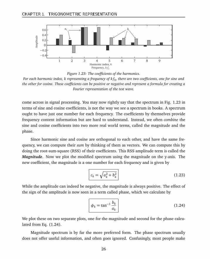
here bk are coefficients of the sine harmonics and ak are the coefficients of the cosine har-monics. We plot these in a bar graph in Fig. 1.23. Both sine and cosine of same frequencyare plotted next to each other for the same harmonic. This is a spectrum that in essencedisplays the recipe for the signal. It tells us how much of each harmonic i.e. its amplitudewe need to recreate the signal.

The Fourier series coefficients tell us how much of each harmonic frequency is containedin our target signal, so they are a measure of its recipe. The coefficients for this reason areanalogous to the spectrum of the signal. Commonly a spectrum is in terms of “Power” butthe coefficients we compute via Fourier analysis are “not” power. They are amplitudes. Theterm spectrum is often used synonymous with power spectrum. One needs to know the typeof spectrum one is plotting or looking at.

In signal processing, the coefficients computed for cosine are called Real and those forsine, Imaginary. Of course, there is nothing imaginary about the coefficients of sine, theyare just as real as the cosine coefficients. It is just one of the many confusing terms we

25


1 2 3 4 5 6 7 8 9

−0.4

−0.2

0

0.2

0.4

0.6

Harmonic index, k

Frequency, k f0

Amplitude

ka

kb

Figure 1.23: The coefficients of the harmonics.For each harmonic index, k representing a frequency of k f0, there are two coefficients, one for sine andthe other for cosine. These coefficients can be positive or negative and represent a formula for creating a

Fourier representation of the test wave.

come across in signal processing. You may now rightly say that the spectrum in Fig. 1.23 interms of sine and cosine coefficients, is not the way we see a spectrum in books. A spectrumought to have just one number for each frequency. The coefficients by themselves providefrequency content information but are hard to understand. Instead, we often combine thesine and cosine coefficients into two more real world terms, called the magnitude and thephase.

Since harmonic sine and cosine are orthogonal to each other, and have the same fre-quency, we can compute their sum by thinking of them as vectors. We can compute this bydoing the root-sum-square (RSS) of their coefficients. This RSS amplitude term is called theMagnitude. Now we plot the modified spectrum using the magnitude on the y-axis. Thenew coefficient, the magnitude is a one number for each frequency and is given by

ck =Ç

a2k + b2

k (1.23)

While the amplitude can indeed be negative, the magnitude is always positive. The effect ofthe sign of the amplitude is now seen in a term called phase, which we calculate by

φk = tan−1 bk

ak(1.24)

We plot these on two separate plots, one for the magnitude and second for the phase calcu-lated from Eq. (1.24).

Magnitude spectrum is by far the more preferred form. The phase spectrum usuallydoes not offer useful information, and often goes ignored. Confusingly, most people make

26


1 2 3 4 5 6 7 8 90

0.2

0.4

0.6

0.8

1

Magnitude

1 2 3 4 5 6 7 8 9−2

−1

0

1

2

Phase, Radians

(a) Magnitude of the harmonics (b) Phase of the harmonics

Harmonic index, k

Frequency, k f0

Harmonic index, k

Frequency, k f0

Figure 1.24: The Magnitude and Phase spectrum.In (a), we see the RSS of both the sine and cosine coefficients, representing the magnitude of that

harmonic frequency. In (b), we compute the phase for each harmonic. The magnitude on the right isusually quite instructive but phase is hard to comprehend as it changes quickly from one frequency to

the next.

no distinction when talking about amplitude or magnitude, often these two terms are usedinterchangeably. The first form, the spectrum based on the real and imaginary coefficients,changes depending on the starting point of the analysis, where the second form, the mag-nitude and the phase are not a function of the starting point. Hence practicing engineersprefer the second from.

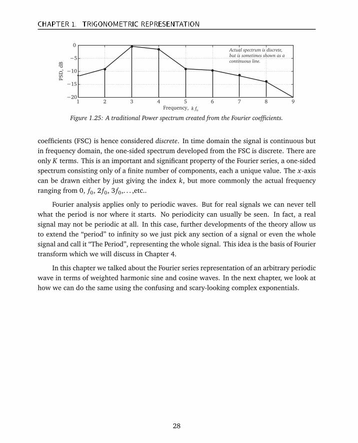
The process of doing the Fourier analysis consists of computing the amplitude of eachharmonic and then from it the magnitude and the phase. In Fig. 1.25 we show a powerspectrum with y-axis given in dBs and shows the power of each harmonic, not the magnitude.To convert a magnitude spectrum to a power spectrum, we use Parseval’s theorem. The tellsus that the total power in a signal is the sum of the powers in each harmonic. The powerin each harmonics is defined as the square of its magnitude. Hence to represent power, yousquare each magnitude value and then compute its dB value by 10 · log(ck)2. Alternately,you can just compute the log10 of the coefficient and multiply it by 20.

Power in the k-th harmonic= 20 log(ck) (1.25)

The power spectrum is often normalized to maximum power, such as bin 3 here. (The bin isa form of identifier of the harmonic.) The level of each component is the dB equivalent of itsratio to the maximum power. All component levels relative to the maximum power, are saidto be a certain number of dBs below the maximum. The maximum level is zero dB, with allother values shown as negative. These values are also called Power Spectral density (PSD)because they are a form of density of the power across a bandwidth.

Looking at the Fourier series coefficients, note that there are just K (the largest k) num-ber of such coefficients, one for each of the harmonics. The spectrum from Fourier series

27


1 2 3 4 5 6 7 8 9−20

−15

−10

−5

0

0k fFrequency,

PSD, dB

Actual spectrum is discrete,

but is sometimes shown as a

continuous line.

Figure 1.25: A traditional Power spectrum created from the Fourier coefficients.

coefficients (FSC) is hence considered discrete. In time domain the signal is continuous butin frequency domain, the one-sided spectrum developed from the FSC is discrete. There areonly K terms. This is an important and significant property of the Fourier series, a one-sidedspectrum consisting only of a finite number of components, each a unique value. The x-axiscan be drawn either by just giving the index k, but more commonly the actual frequencyranging from 0, f0, 2 f0, 3 f0,. . . ,etc..

Fourier analysis applies only to periodic waves. But for real signals we can never tellwhat the period is nor where it starts. No periodicity can usually be seen. In fact, a realsignal may not be periodic at all. In this case, further developments of the theory allow usto extend the “period” to infinity so we just pick any section of a signal or even the wholesignal and call it “The Period”, representing the whole signal. This idea is the basis of Fouriertransform which we will discuss in Chapter 4.

In this chapter we talked about the Fourier series representation of an arbitrary periodicwave in terms of weighted harmonic sine and cosine waves. In the next chapter, we look athow we can do the same using the confusing and scary-looking complex exponentials.

28


Summary of Chapter 1In this chapter, we introduced the concept of using sinusoids to represent an arbitrary

periodic wave. We also introduced the concept of the fundamental frequency and its har-monics. The Fourier series representation consists of finding unique weightings of theseharmonics to represent a particular periodic wave. These weightings are called the Fourierseries Coefficients (FSC). These coefficients when plotted as a function of the frequency rep-resent the spectrum of the signal. The spectrum calculated using FSC is discrete althoughthe signal is continuous in time.

Terms used in this chapter:

• Fundamental frequency - the smallest frequency of the signal to be represented byFourier series.

• Harmonic frequencies - All integer multiples of the fundamental frequency.• Sinusoids - sine or cosine wave.• Harmonic coefficients - The amplitude of a harmonic.• Real and imaginary - Cosine is said to exist in the real plane and sine in the imaginary

plane.• Magnitude - the RSS value of the amplitudes of the sine and cosine of a particular

harmonic. It is always positive.• Phase - the stating value of a wave at t = 0, often specified in radians.

1. The most common trigonometric form of the Fourier series is given by

f (t) = a0 +∞∑

k=1

ak cos(2π fk t) +∞∑

k=1

bk sin(2π fk t)

2. The coefficients of the Fourier series are easily computed by

a0 =1T0

∫ T0

0

f (t)d t

bk =2T0

∫ T0

0

f (t) sin(kω0 t)d t

ak =2T0

∫ T0

0

f (t) cos(kω0 t)d t

3. Many periodic signals can be represented by weighted sum of harmonics sinusoids.The representation is an estimation and may not be an exact replication.

4. Harmonic sinusoids are orthogonal to each other, hence the integral of their products(or cross product) is zero.

29


5. The linearity property of the Fourier series implies that a change of the coefficients ofone harmonic does not effect the coefficients of the other harmonics.

6. A time or phase shift of the signal does not effect the magnitude of the coefficients.7. To synthesize a signal based on Fourier series, we pick a fundamental frequency first.

All harmonics are integer multiples of the fundamental.8. We designate harmonics by letter k. Hence for all integer k, all k f0 frequencies are

harmonics of the fundamental frequency f0.9. The Fourier analysis means to find the Fourier coefficients of the Fourier series.

10. The Fourier coefficients are discrete since the harmonics are discrete. Hence the spec-trum of a periodic continuous-time signal is discrete.

11. A spectrum can be a spectrum of amplitude, magnitude or of power. These are not thesame thing.

Questions1. Can you state in words the principal behind Fourier series.2. What is the third harmonic of a sinusoid of frequency 3 Hz.3. Can any signal have harmonics?4. Why is one harmonic orthogonal to another. What trigonometric property tells us that

this is true?5. If we add three non-harmonic sinusoids together, is the resulting signal periodic?6. If we multiply the amplitude of a signal by a non-linear value, what effect will that

have on its frequency?7. A change in phase of a cosine wave means it is still orthogonal to a sine wave of the

same frequency, true or false?8. What is the maximum amplitude of N harmonic cosine waves added together. What is

it for sine waves.9. We need to represent a wave that starts at time t = 0. What type of harmonics will be

in its representation.10. Summation of odd and even waves can be used to create any waveform we want, true

or not?11. Is Fourier series representation an accurate representation of a wave? Why not?12. Can we create a Fourier series representation of any wave?13. Why do we consider the set of harmonics a basis set? What constitutes a basis set?14. Sine and cosine waves are a basis set for Fourier analysis. Can you give an example of

another set of basis functions.15. What quality of sine and cosine makes them suitable as a basis set?16. Fourier series analysis is considered a linear process. Why?

30


17. What do the coefficients of a Fourier series represent? What does the a0 coefficientrepresent?

18. What is the Fourier series representation of this signal? s = A+ B sin(2π f t).19. We want to compute the FSC coefficients of this signal. s = sin(6.5t) − cos(4.75t).

What should we pick as the fundamental frequency?20. If the target wave is shifted by a certain phase, what happens to its coefficients?21. How many coefficients would you need to describe this wave? x(t) = 2+ B sin(4πt +

π/2)− cos(12πt). Find the coefficients of this above signal.22. What is the fundamental period of this FS representation. x(t) = 2/π(sin(4πt) +(1/3)sin(12πt) + (1/5)sin(20πt) + (1/7)sin(28πt). What are the coefficients of thefirst four cosine and sine coefficients.

23. Given these equations, what are the Fourier series coefficients, a0, a1, a2 for each case.

(a) y =12+

34

sin(πx)−35

cos(2πx).

(b) y =34

cos(2πx)−35

cos(3πx).

24. What is the difference between amplitude and magnitude?25. The amplitude of a harmonics varies from -1 v to +1 v. What is the magnitude of the

harmonic? What is the power of the harmonic? What is the value of the power in dBs?26. Examine Fig. 1.11 and give first four coefficients of the even square wave.

31


32

Intuitive Guide to Fourier...

Documents

Transcript of Intuitive Guide to Fourier...