Interpreting Line Drawings as Three-Dimensional...
42
ARTIFICIAL INTELLIGENCE 75 Interpreting Line Drawings as Three-Dimensional Surfaces H.G. Barrow and J.M. Tenenbaum* Artificial Intelligence Center, SRI International, Menlo Park, CA 94025, U.S.A. ABSTRACT Understanding how line drawings convey tri-dimensionality is of fundamental importance in explaining surface perception when photometry is either uninformative or too compex to model analytically. We put forward here a computational model for interpreting line drawings as three-dimensional surfaces, based on constraints on local surface orientation along extremal and discontinuity boun- daries. Specific techniques are described for two key processes recovering the three-dimensional conformation of a space curve (e.g., a surface boundary) from its two-dimensional projection in an image, and interpolating smooth surfaces from orientation constraints along extremal boundaries. The relevance of the model to a general theory of low-level vision is discussed. 1. Introduction Recent research in computational vision has sought to understand some of the principles underlying early stages of visual processing in both man and machine. An important function of early vision appears to be the trans- formation of brightness information in the input image into an intermediate representation that describes the intrinsic characteristics (depth, orientation, reflectance, color, and so on) of the three-dimensional surface element at each point in the image [1-4]. Support for this idea comes from four sources: (1) The observed ability of humans to determine these characteristics, regardless of viewing conditions or familiarity with the scene. (2) The direct value of such characteristics to applications like manipulation and obstacle avoidance. (3) The utility of such a representation for facilitating higher-level processing (e.g. segmentation or object recognition) in computer vision systems. (4) Theoretical *Both authors are now at the Artificial Intelligence Research Laboratory, Fairchild Camera and Instrument Corporation, Palo Alto, CA 94304. Artificial Intelligence 17 (1981) 75-116 0004-3702/81/0000-0000/$02.50 © North-Holland
Transcript of Interpreting Line Drawings as Three-Dimensional...

ARTIFICIAL INTELLIGENCE 75
Interpreting Line Drawings asThree-Dimensional Surfaces
H.G. Barrow and J.M. Tenenbaum*Artificial Intelligence Center, SRI International, MenloPark, CA 94025, U.S.A.
ABSTRACTUnderstanding how line drawings convey tri-dimensionality is of fundamental importance in explainingsurface perception when photometry is either uninformative or too compex to model analytically.
We put forward here a computational model for interpreting line drawings as three-dimensionalsurfaces, based on constraints on local surface orientation along extremal and discontinuity boun- daries. Specific techniques are described for two key processes recovering the three-dimensionalconformation of a space curve (e.g., a surface boundary) from its two-dimensional projection in an image, and interpolating smooth surfaces from orientation constraints along extremal boundaries. Therelevance of the model to a general theory of low-level vision is discussed.
1. Introduction
Recent research in computational vision has sought to understand some of theprinciples underlying early stages of visual processing in both man and machine. An important function of early vision appears to be the trans- formation of brightness information in the input image into an intermediaterepresentation that describes the intrinsic characteristics (depth, orientation, reflectance, color, and so on) of the three-dimensional surface element at each point in the image [1-4]. Support for this idea comes from four sources: (1) Theobserved ability of humans to determine these characteristics, regardless of viewing conditions or familiarity with the scene. (2) The direct value of suchcharacteristics to applications like manipulation and obstacle avoidance. (3) The utility of such a representation for facilitating higher-level processing (e.g.segmentation or object recognition) in computer vision systems. (4) Theoretical
*Both authors are now at the Artificial Intelligence Research Laboratory, Fairchild Camera andInstrument Corporation, Palo Alto, CA 94304.
Artificial Intelligence 17 (1981) 75-116
0004-3702/81/0000-0000/$02.50 © North-Holland

76 H.G. BARROW AND J.M. TENENBAUM
arguments that such descriptions could, in fact, be recovered by nonpurposive,noncognitive processes, at least for simple scene domains [4].
In principle, information about surfaces can be obtained from many sources:stereopsis, motion parallax, texture gradient, and shading, to name a few. Each of these cues, however, is valid only for a particular class of situations. For example, stereopsis and motion parallax require multiple images; determining surface shape from texture requires statistical regularity of the textural ele- ments. Analytic techniques for determining shape from shading require ac- curate modeling of the incident illumination and surface photometry, which is difficult to do for most natural scenes.
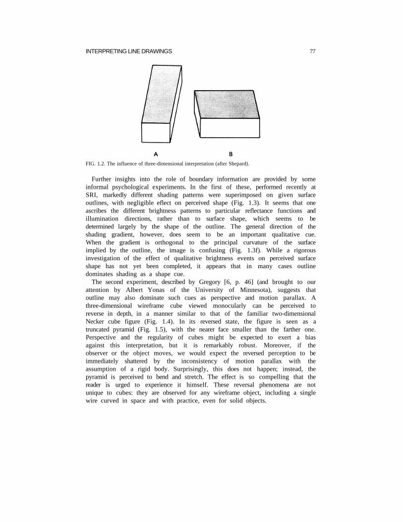
Even in the absence of such powerful analytic cues, much valuable in- formation about surface structure is still available. In particular, much is conveyed by brightness discontinuities, which occur wherever there are dis-continuities in incident illumination (at shadow boundaries), reflectance (at surface markings), or surface orientation (at surface boundaries). The significance of surface discontinuities alone is evident from our ability to infer the three-dimensional structure of objects depicted in line drawings, such as Fig. 1.1. Boundary information is such a fundamental cue to tri-dimensionality that it is hard for humans to suppress it. The shaded parallelograms in Fig. 1.2 are two-dimensionally congruent, but appear strikingly different because their three-dimensional interpretations are so different (from [5]).
FIG. 1.1. Line drawing of a three-dimensional scene.Surface and boundary structure are distinctly perceived despite the ambiguity inherent in imaging
process.
INTERPRETING LINE DRAWINGS 77
FIG. 1.2. The influence of three-dimensional interpretation (after Shepard).
Further insights into the role of boundary information are provided by some informal psychological experiments. In the first of these, performed recently at SRI, markedly different shading patterns were superimposed on given surface outlines, with negligible eflect on perceived shape (Fig. 1.3). It seems that oneascribes the different brightness patterns to particular reflectance functions andillumination directions, rather than to surface shape, which seems to be determined largely by the shape of the outline. The general direction of the shading gradient, however, does seem to be an important qualitative cue. When the gradient is orthogonal to the principal curvature of the surface implied by the outline, the image is confusing (Fig. 1.3f). While a rigorousinvestigation of the effect of qualitative brightness events on perceived surface shape has not yet been completed, it appears that in many cases outline dominates shading as a shape cue.
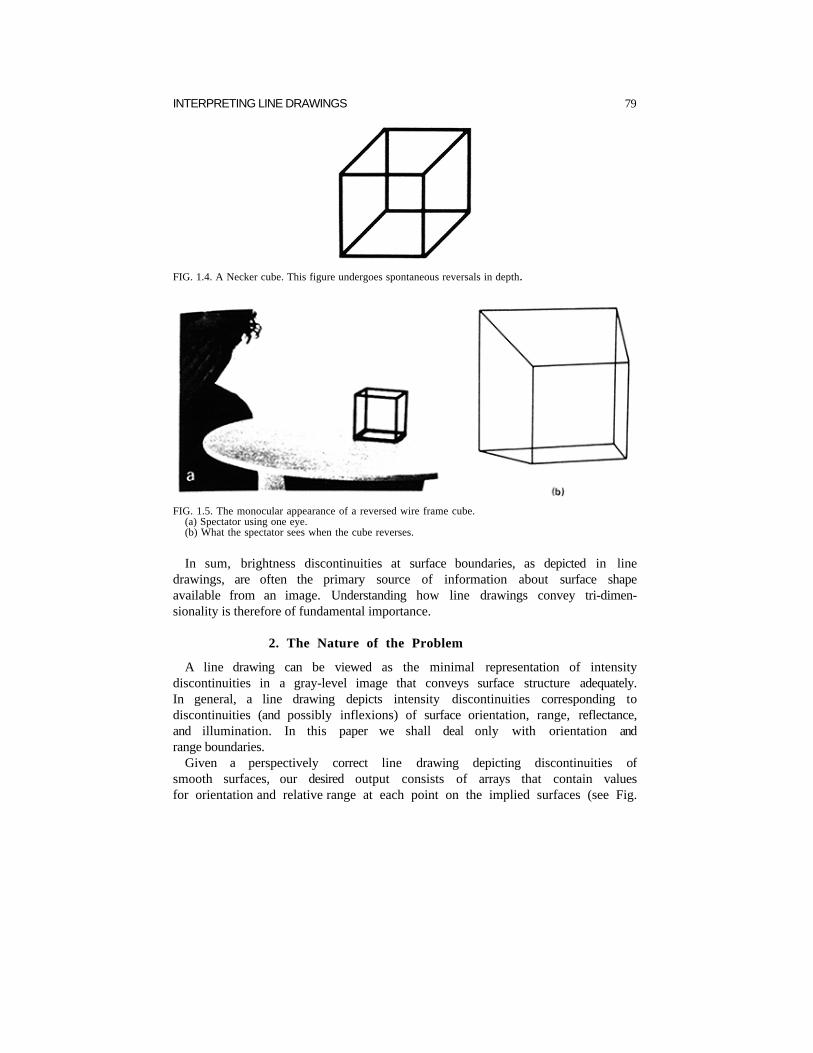
The second experiment, described by Gregory [6, p. 46] (and brought to our attention by Albert Yonas of the University of Minnesota), suggests that outline may also dominate such cues as perspective and motion parallax. A three-dimensional wireframe cube viewed monocularly can be perceived to reverse in depth, in a manner similar to that of the familiar two-dimensional Necker cube figure (Fig. 1.4). In its reversed state, the figure is seen as a truncated pyramid (Fig. 1.5), with the nearer face smaller than the farther one.Perspective and the regularity of cubes might be expected to exert a bias against this interpretation, but it is remarkably robust. Moreover, if the observer or the object moves, we would expect the reversed perception to beimmediately shattered by the inconsistency of motion parallax with the assumption of a rigid body. Surprisingly, this does not happen; instead, the pyramid is perceived to bend and stretch. The effect is so compelling that the reader is urged to experience it himself. These reversal phenomena are not unique to cubes: they are observed for any wireframe object, including a single wire curved in space and with practice, even for solid objects.

78 H.G. BARROW AND J.M. TENENBAUM
FIG 1.3. An informal experiment demonstrating the relative importance of shading and boundary curves as determinants of surface shape
Different one-dimensional shading gradients appear to have little effect on the perceived shape of a surface defined by a given outline. The direction of the shading gradient does seem important,however, as a qualitative cue for line sorting. Fig. (f), where the shading gradient runs orthogonal to the cylindrical curvature implied by the contour is difficult to interpret.
(a) A cylindrical patch in silhouette.(b) A cylindrical patch with shading falling off linearly on both sides of the highlight.(c) A cylindrical patch with shading falling off quadratically from the highlight.(d) A cuspate surface with shading falling off linearly.(ei A cuspate surface with shading falling off quadratically.(f) A cylindncal patch with inconsistent shading.
INTERPRETING LINE DRAWINGS 79
FIG. 1.4. A Necker cube. This figure undergoes spontaneous reversals in depth.
FIG. 1.5. The monocular appearance of a reversed wire frame cube.(a) Spectator using one eye.(b) What the spectator sees when the cube reverses.
In sum, brightness discontinuities at surface boundaries, as depicted in linedrawings, are often the primary source of information about surface shape available from an image. Understanding how line drawings convey tri-dimen- sionality is therefore of fundamental importance.
2. The Nature of the Problem
A line drawing can be viewed as the minimal representation of intensitydiscontinuities in a gray-level image that conveys surface structure adequately. In general, a line drawing depicts intensity discontinuities corresponding todiscontinuities (and possibly inflexions) of surface orientation, range, reflectance, and illumination. In this paper we shall deal only with orientation and range boundaries.
Given a perspectively correct line drawing depicting discontinuities of smooth surfaces, our desired output consists of arrays that contain values for orientation and relative range at each point on the implied surfaces (see Fig.

80 H.G. BARROW AND J.M. TENENBAUM
FIG. 2.1. An input/output model of line drawing interpretation.
2.1). These output arrays are analogous to our intrinsic images [4] or Marr’s 2.5-D sketch [3].
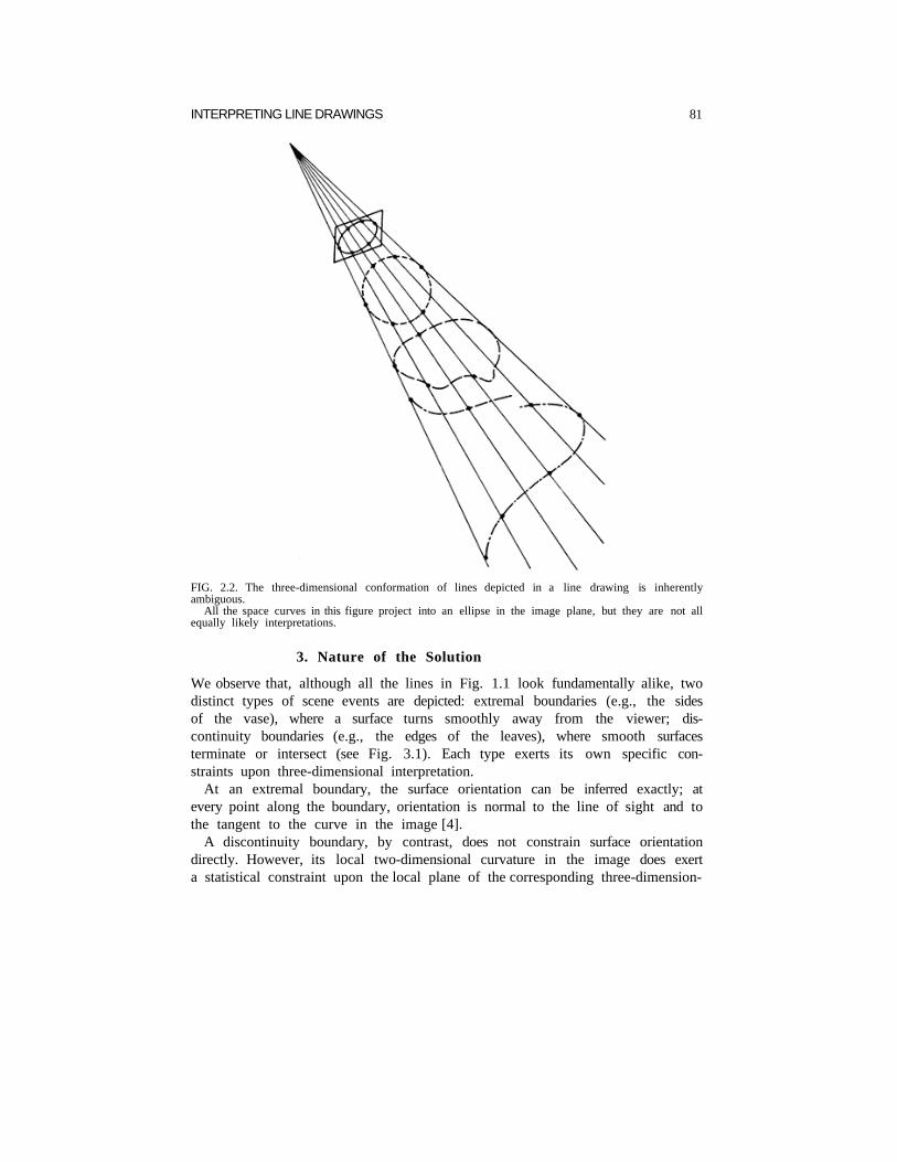
The central problem in perceiving line drawings is one of ambiguity. Since each point in an image determines only a ray in space and not a unique point, a two-dimensional line in the image could, in theory, correspond to a possibleprojection of an infinitude of three-dimensional space curves (see Fig. 2.2). Yet people are not aware of this massive ambiguity. When they are asked to provide a three-dimensional interpretation of an ellipse, the overwhelming response is a tilted circle, not some bizarrely twisting curve (or even a discontinuous one) that has the same image. What assumptions about the scene and the imaging process are invoked to constrain this unique interpretation?
In previous work, attempts were made to resolve this ambiguity by inter- preting line drawings in terms of such high-level knowledge as object models [7, 8], junction catalogs [9, 10, 11], or generalized cylinders [12]. Following thisapproach, the interpretation of an ellipse is commonly explained in terms of aprototypical circle. However, this cannot account for the significant observation that, for any given view of an arbitrary space curve, only two of the infinite set of possible interpretations are normally perceived—the (approximately) correct one and a single Necker inverse. There is thus reason to believe that the human visual stystem relies on constraints that are more fundamental than prototypes.
INTERPRETING LINE DRAWINGS 81
FIG. 2.2. The three-dimensional conformation of lines depicted in a line drawing is inherently ambiguous.
All the space curves in this figure project into an ellipse in the image plane, but they are not all equally likely interpretations.
3. Nature of the Solution
We observe that, although all the lines in Fig. 1.1 look fundamentally alike, twodistinct types of scene events are depicted: extremal boundaries (e.g., the sides of the vase), where a surface turns smoothly away from the viewer; dis- continuity boundaries (e.g., the edges of the leaves), where smooth surfaces terminate or intersect (see Fig. 3.1). Each type exerts its own specific con- straints upon three-dimensional interpretation.
At an extremal boundary, the surface orientation can be inferred exactly; at every point along the boundary, orientation is normal to the line of sight and to the tangent to the curve in the image [4].
A discontinuity boundary, by contrast, does not constrain surface orientation directly. However, its local two-dimensional curvature in the image does exert a statistical constraint upon the local plane of the corresponding three-dimension-

82 H.G. BARROW AND J.M. TENENBAUM
FIG. 3.1. Different edge types in a line drawing.
al space curve, and thus upon relative depth along the curve. Moreover, the surface normal at each point along the boundary is then constrained to be orthogonal to the three-dimensional tangent in the plane of the space curve, leaving only one degree of freedom unknown; i.e., the surface normal is hinged to the tangent free to swing about it as shown in Fig. 3.2.
The ability to infer three-dimensional surface structure from extremal anddiscontinuity boundaries suggests a three-step model for line drawing inter- pretation (see Fig. 3.3), analogous to those involved in our intrinsic-image model [4]: line sorting, three-dimensional boundary interpretation, and surface
FIG. 3.2. Surface orientation is constrained to one degree of freedom along discontinuity boun- daries.

INTERPRETING LINE DRAWINGS 83
FIG. 3.3. A model for interpretation of line drawings.
interpolation. Each line is first classified according to the type of surface boundary it represents (extremal or discontinuity). Surface contours are inter- preted as three-dimensional space curves, providing relative 3-D distances along each curve; local surface normals are assigned along the extremal boundaries. Finally, three-dimensional surfaces consistent with these boundaryconditions are constructed by interpolation. (For an alternative model, see [13].)
4. Line Sorting
4.1. Line classification
The first step in interpreting an ideal line drawing is to classify the various linesaccording to the type of surface boundary they represent. Each type involves different constraints in arriving at a three-dimensional interpretation, and imposes different boundary conditions. The problem is that all lines in a line
84 H.G. BARROW AND J.M. TENENBAUM
drawing look fundamentally alike. How, then, are we able to distinguish the extremal boundaries and surface contours in an image like Fig. 1.1?
The two principal bases for classifying lines are local cues provided by line junctions and global cues provided by geometric relations, such as symmetry and parallelism. A third possibility, considered less likely on combinatorial grounds, is that line classification is performed in tandem with surface inter- pretation to optimize some joint measure of boundary and surface smoothness.
4.1.1. Junctions
Junctions were first used for line labeling by Huffman [9], Clowes [14], and Waltz [10]. They systematically enumerated the surface intersections that could occur in scenes composed of trihedral solids and the corresponding line junctions that would result from various viewpoints. Catalogs were produced listing for each type of junction sets of possible interpretations of the emanat- ing lines. Line labeling was accomplished by using the catalogs to assign all locally possible interpretations to the lines at each junction and then using a global constraint satisfaction process to resolve ambiguities.
To those familiar with this research, an extension to arbitrarily curved objects is, at first thought, overwhelming. Waltz's catalog, for example, enu- merated nearly 3000 physical interpretations of the junctions in line drawings of trihedral scenes. Turner [11] needed a catalog many times larger to accom- modate solids with parabolic and elliptic surfaces. Waltz and Turner, however,attempted to classify lines into numerous detailed categories, such as convex, concave, crack, and shadow. For our purposes only two classes are significant:extremal boundaries which constrain surface orientation, and surface contours, which constrain relative distance. This drastically reduces the number of junction types.
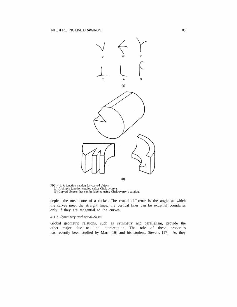
Fig. 4.1a shows a simple junction catalog recently published by Chakravarty [15] that can handle a wide variety of curved objects, including all those shown in Fig. 4.1b. These junctions exert remarkably strong local constraints upon theinterpretation of lines as extremal, occluding, or intersecting edges. Junction S, for example, implies a vertex formed by an extremal edge that meets intersec- ting and occluding edges, as occurs where the side of a cylinder meets the visible end; junction A implies an extremal edge meeting the hidden end; junction W suggests the intersection of two surfaces bounded by discontinuity edges; T junctions play their usual role of an occlusion cue, indicating relative depth. These junctions also resolve figure-ground ambiguities in regard to which surface(s) a line bounds.1
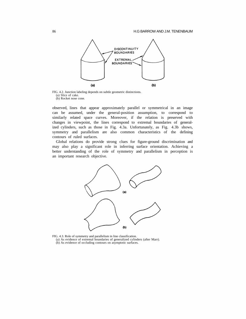
One caveat about using junctions for labeling line drawings of curved objects is that determination of the junction category may depend on subtle variation in geometry that are difficult to distinguish in practice. For example, Fig. 4.2a, which depicts a slice of cake, can easily be confused with Fig. 4.2b, which
1For a derivation of some of the catalog entries from a general position assumption, see [29].
INTERPRETING LINE DRAWINGS 85
FIG. 4.1. A junction catalog for curved objects.(a) A simple junction catalog (after Chakravarty).(b) Curved objects that can be labeled using Chakravarty’s catalog.
depicts the nose cone of a rocket. The crucial difference is the angle at which the curves meet the straight lines; the vertical lines can be extremal boundaries only if they are tangential to the curves.
4.1.2. Symmetry and parallelism
Global geometric relations, such as symmetry and parallelism, provide the other major clue to line interpretation. The role of these properties has recently been studied by Marr [16] and his student, Stevens [17]. As they
86 H.G BARROW AND J.M. TENENBAUM
FIG. 4.2. Junction labeling depends on subtle geometric distinctions.(a) Slice of cake.(b) Rocket nose cone.
observed, lines that appear approximately parallel or symmetrical in an image can be assumed, under the general-position assumption, to correspond to similarly related space curves. Moreover, if the relation is preserved with changes in viewpoint, the lines correspond to extremal boundaries of general- ized cylinders, such as those in Fig. 4.3a. Unfortunately, as Fig. 4.3b shows,symmetry and parallelism are also common characteristics of the defining contours of ruled surfaces.
Global relations do provide strong clues for figure-ground discrimination and may also play a significant role in inferring surface orientation. Achieving a better understanding of the role of symmetry and parallelism in perception is an important research objective.
FIG. 4.3. Role of symmetry and parallelism in line classification.(a) As evidence of extremal boundaries of generalized cylinders (after Marr).(b) As evidence of occluding contours on asymptotic surfaces.

INTERPRETING LINE DRAWINGS 87
5. Three-Dimensional Line Interpretation
Once lines are classified as physical boundaries, the next step is to determine the constraints (i.e. boundary conditions) they impose on three-dimensional surfaces.
In principle, extremal boundaries are especially simple to interpret; since the surface normal is orthogonal to both the line of sight and the curve in the image, it is determined uniquely at every point. In practice, however, the normal to a noisy, quantized image curve cannot be ascertained with a high degree of accuracy. Some refinement of the estimate of surface normal, based on the results of the subsequent surface interpolation process, may thus be necessary. This problem is dealt with further in Section 6.
Surface discontinuity boundaries constrain the surface normal to one degree of freedom, but first it is necessary to recover the three-dimensional conformation of the corresponding space curve. To recover this conformation from the two-dimensional image, we invoke two domain-independent assumptions: sur- face smoothness and general position.
The smoothness assumption implies that the space curve bounding a surface will also be smooth. Since continuity is preserved under projection, a smooth curve in space results in a smooth curve in the image. However, because of theinherent ambiguity introduced in projection to a lower dimension, it does notnecessarily follow that a smooth image curve must correspond to a smooth space curve. This inference requires the additional assumption that a scene is being viewed from a general position, so that perceived smoothness is not an accident of viewpoint. A general-viewpoint assumption is quite reasonable. In Fig. 2.2, for example, the sharply receding curve is projected into a smooth ellipse from only one viewpoint. Thus, such a curve would be a highly improbable three-dimensional interpretation of an ellipse.
The problem now is to determine which smooth space curve is most likely. Strictly speaking, a maximum-likelihood decision requires knowledge of the nature of the process that generated the space curve. For example, is it a bent wire, the edge of a curved ribbon, or the intersection of two soap films? In the absence of such knowledge, it is reasonable to assume that a given image curve is most likely to correspond to the smoothest possible projectively equivalent space curve. This conjecture appears consistent with human perception [18]: The ellipse in Fig. 2.2 is almost universally perceived as a tilted circle. In many cases, it is also justified on the ecological ground that surfaces tend to assume smooth, minimal-energy configurations.
5.1. Measures of smoothness
The smoothness of a space curve is expressed quantitatively in terms of its intrinsic characteristics, such as differential curvature (k) and torsion (t), as well as vectors giving intrinsic axes of the curve: tangent (T), principal normal (N),

88 H.G. BARROW AND J.M. TENENBAUM
FIG. 5.1. Intrinsic characteristics of a space curve.
and binormal (B) (See Fig. 5.1). We define k as the reciprocal of the radius of the osculating circle at each point on the curve. N is the vector from the center of curvature normal to the tangent. B, the vector cross product of T and N, defines the normal to the plane of the curve. Torsion t is the spatial derivative of the binormal, and expresses the degree to which the curve twists out of a plane. (For further details, see any standard text on vector differential geometry.)
An obvious measure of the smoothness of a space curve is uniformity of curvature. Thus, one might seek the space curve corresponding to a given image curve for which the integral of k ' (the spatial derivative of k) was minimal. This alone, however, is insufficient since the integral of k ' could be made arbitrarily small by stretching out the space curve so that it approaches a twisting straight line (see Fig. 5.2). Nor does uniformity of curvature indicate whether a circular arc in the image should correspond to a 3-D circular arc or to part of a helix. A necessary additional constraint in both cases is that the space curve corresponding to a given image curve should be as planar as
FIG. 5.2. An interpretation that increases uniformity of curvature.
INTERPRETING LINE DRAWINGS 89
possible or, more precisely, that the integral of its torsion should be minimized.Integral (1) expresses both the smoothness and planarity of a space curve in
terms of a single, locally computed differential measure d(kB)/ds. To interpret an image curve, it is thus necessary to find the projectively equivalent space curve that minimizes this integral:
d kB
dsds k k t ds
( )'
= +( )∫ ∫
22 2 2 . (1)
Intuitively, minimizing (1) corresponds to finding the three-dimensional projection of an image curve that most closely approximates a planar, circular arc for which k' and t are both everywhere zero.
5.2. Recovery techniques
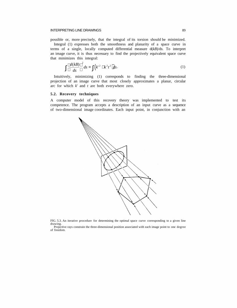
A computer model of this recovery theory was implemented to test its competence. The program accepts a description of an input curve as a sequence of two-dimensional image coordinates. Each input point, in conjunction with an
FIG. 5.3. An iterative procedure for determining the optimal space curve corresponding to a given linedrawing.
Projective rays constrain the three-dimensional position associated with each image point to one degreeof freedom.

90 H.G. BARROW AND J.M. TENENBAUM
an assumed center of projection, defines a ray in space along which the corresponding space curve point is constrained to lie (Fig. 5.3). The program can adjust the distance associated with each space curve point by sliding it along its ray like a bead on a wire. The 3-D coordinates of three consecutive points on the curve determine a circle in space, the normal to which gives the direction of B, and the radius of which gives 1/k, as shown in Fig. 5.4. From these, a discrete approximation to the smoothness measure, d(kB)/ds, can be obtained.
An iterative optimization procedure was used to determine the configuration of points that minimized the integral in (1). The optimization proceeded byindependently adjusting each space curve point to minimize d(kB)/ds locally. (Note that local perturbations of z have only local effects on curvature and torsion.)
The program was tested using input coordinates synthesized from known 3-D space curves, so that results could be readily evaluated. Correct 3-D inter- pretations were produced for simple and closed curves, such as an ellipse, which was interpreted as a tilted circle. However, convergence was slow and somewhat dependent on the initial choice of z-values. For example, the program had difficulties converging to the ‘tilted-circle’ interpretation of an ellipse if it had been started with z-values either all in a plane parallel to the image plane or randomized to be highly nonplanar.
To overcome these deficiencies, we experimented with an alternative ap- proach based on ellipse-fitting that involved more local constraints. A smooth space curve can be approximated locally by arcs of circles. Circular arcs are projected as elliptic arcs in an image. We already know that an ellipse in the image corresponds to a circle in three-dimensional space; the plane of the circle is obtained by rotating the plane of the ellipse ahout its major axis by an angle
FIG. 5.4. Discrete approximation to B, T, k from 3 points.
INTERPRETING LINE DRAWINGS 91
equal to arc cos(minor axis/major axis). The relative depth at points along a surface contour can thus be established, in principle, by fitting an ellipse locally (five points suffice to fit a general conic), and then projecting the local curve fragment back onto the plane of the corresponding circular arc of the space curve. If we assume orthographic projection, a simple linear equation results, relating differential depth along the curve to differential changes in its imagecoordinates, as shown in (2):
dz = a ⋅ dx + b ⋅ dy. (2)
The ellipse-fitting method yielded correct 3-D interpretations for ideal image data but, not surprisingly, broke down because of large fitting errors when small amounts of quantization noise were added. Presently under investigation are several alternative approaches that attempt to overcome these problems byexploiting global properties (e.g., segmenting the curve and fitting ellipses to large fragments) and by integrating boundary interpretation with surface in- terpolation.
5.3. Recovery of polyhedra
Techniques for reconstructing three-dimensional curves based on such criteria as uniformity of curvature break down when the lines involved are not smooth. An important special case concerns figures involving straight lines (polygons and polyhedra). The general-position assumption implies that a straight line in the image corresponds to a straight line in space. For a single line, since curvature is everywhere zero, inclination to the image plane is unconstrained. For figures with multiple straight lines, however, an analog to curvature is provided by the angles between the lines, thus allowing a three-dimensionalconformation to be recovered.
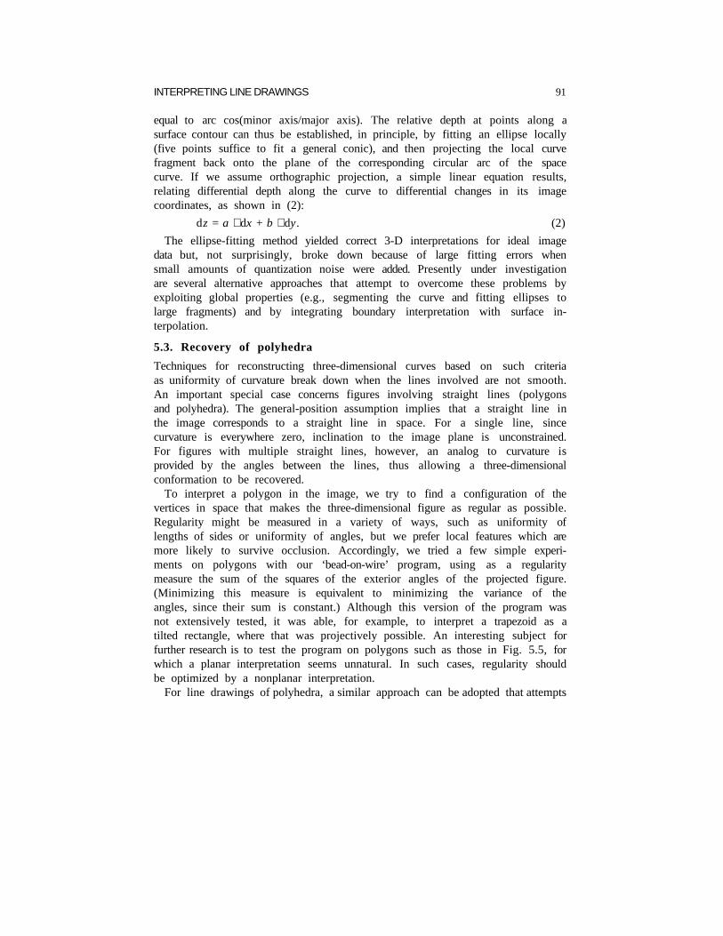
To interpret a polygon in the image, we try to find a configuration of the vertices in space that makes the three-dimensional figure as regular as possible.Regularity might be measured in a variety of ways, such as uniformity of lengths of sides or uniformity of angles, but we prefer local features which are more likely to survive occlusion. Accordingly, we tried a few simple experi- ments on polygons with our ‘bead-on-wire’ program, using as a regularity measure the sum of the squares of the exterior angles of the projected figure.(Minimizing this measure is equivalent to minimizing the variance of the angles, since their sum is constant.) Although this version of the program was not extensively tested, it was able, for example, to interpret a trapezoid as a tilted rectangle, where that was projectively possible. An interesting subject for further research is to test the program on polygons such as those in Fig. 5.5, forwhich a planar interpretation seems unnatural. In such cases, regularity should be optimized by a nonplanar interpretation.
For line drawings of polyhedra, a similar approach can be adopted that attempts

92 H.G. BARROW AND J.M. TENENBAUM
FIG. 5.5. ‘Non-planar’ polygons.
attempts to find the configuration of vertices that makes the three-dimensionalreconstruction as regular as possible. Each vertex of the drawing has an estimated z value, which can be adjusted (by sliding the vertex along a line of sight). Adjustments are made to optimize some global measure of regularity. We have tried using the following: the sum of the squares of angles of faces (which tends to make all angles equal); the sum of the squares of two pi minus the sum of angles at a vertex (which tends to equalize an analog of Gaussian curvature at the vertices); the sum of squares of cosines of face angles (which tends to produce right angles). All these measures have been tried on simple drawings of wireframe tetrahedra, and they all produce similar results: a fairly regular tetrahedral solid.
The program optimizes a measure that is independent of viewpoint and thus tends to produce regular figures. While this result is satisfying, there is evidence that the human visual system is not so objective. If a subject views a nearlysymmetrical figure, such as Fig. 5.6, resembling a view of a tetrahedron resting on a table and seen from above, he does not perceive a truly regular solid. Instead he perceives the central vertex as an approximate cubical corner; hence the height of the pyramid produced is less than that of a true tetrahedron. Thisphenomenon is revealing and worthy of further investigation.
FIG. 5.6. Tetrahedron (top view).
INTERPRETING LINE DRAWINGS 93
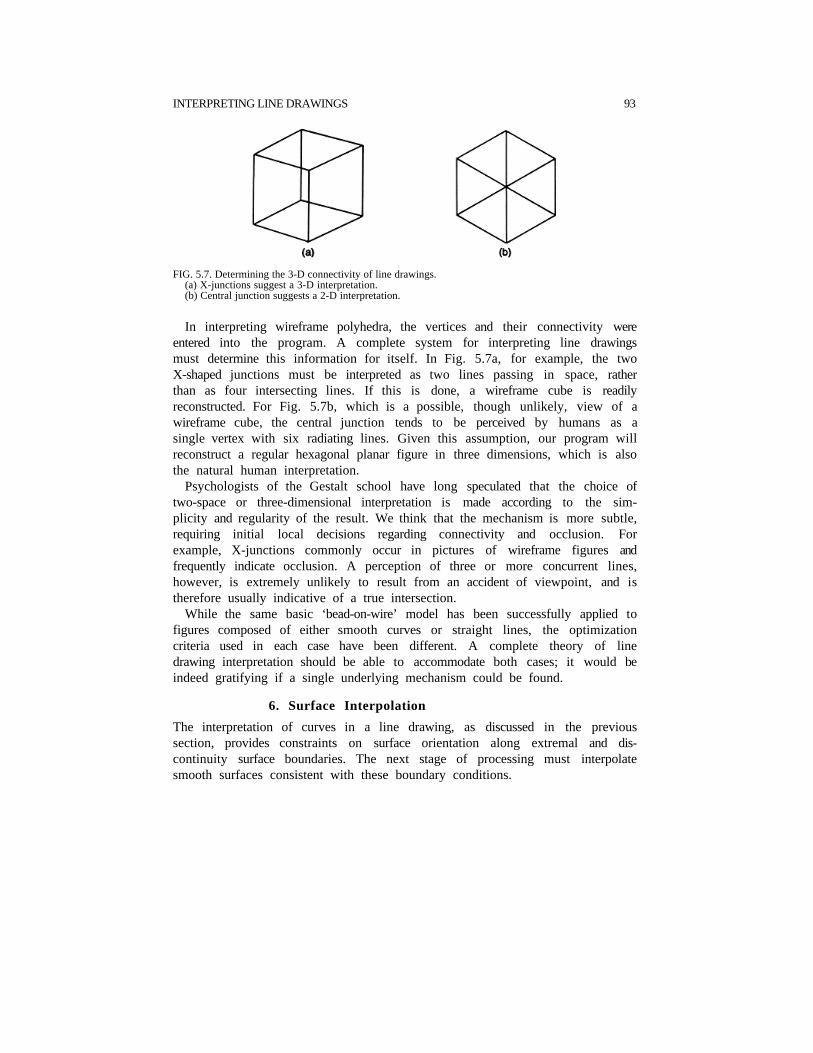
FIG. 5.7. Determining the 3-D connectivity of line drawings.(a) X-junctions suggest a 3-D interpretation.(b) Central junction suggests a 2-D interpretation.
In interpreting wireframe polyhedra, the vertices and their connectivity were entered into the program. A complete system for interpreting line drawings must determine this information for itself. In Fig. 5.7a, for example, the two X-shaped junctions must be interpreted as two lines passing in space, rather than as four intersecting lines. If this is done, a wireframe cube is readily reconstructed. For Fig. 5.7b, which is a possible, though unlikely, view of awireframe cube, the central junction tends to be perceived by humans as a single vertex with six radiating lines. Given this assumption, our program willreconstruct a regular hexagonal planar figure in three dimensions, which is also the natural human interpretation.
Psychologists of the Gestalt school have long speculated that the choice of two-space or three-dimensional interpretation is made according to the sim- plicity and regularity of the result. We think that the mechanism is more subtle,requiring initial local decisions regarding connectivity and occlusion. For example, X-junctions commonly occur in pictures of wireframe figures and frequently indicate occlusion. A perception of three or more concurrent lines, however, is extremely unlikely to result from an accident of viewpoint, and is therefore usually indicative of a true intersection.
While the same basic ‘bead-on-wire’ model has been successfully applied to figures composed of either smooth curves or straight lines, the optimization criteria used in each case have been different. A complete theory of line drawing interpretation should be able to accommodate both cases; it would be indeed gratifying if a single underlying mechanism could be found.
6. Surface Interpolation
The interpretation of curves in a line drawing, as discussed in the previous section, provides constraints on surface orientation along extremal and dis- continuity surface boundaries. The next stage of processing must interpolate smooth surfaces consistent with these boundary conditions.
94 H.G. BARROW AND J.M. TENENBAUM
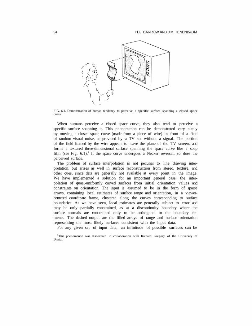
FIG. 6.1. Demonstration of human tendency to perceive a specific surface spanning a closed space curve.
When humans perceive a closed space curve, they also tend to perceive a specific surface spanning it. This phenomenon can be demonstrated very nicely by moving a closed space curve (made from a piece of wire) in front of a field of random visual noise, as provided by a TV set without a signal. The portion of the field framed by the wire appears to leave the plane of the TV screen, and forms a textured three-dimensional surface spanning the space curve like a soap film (see Fig. 6.1).2 If the space curve undergoes a Necker reversal, so does theperceived surface.
The problem of surface interpolation is not peculiar to line drawing inter- pretation, but arises as well in surface reconstruction from stereo, texture, and other cues, since data are generally not available at every point in the image. We have implemented a solution for an important general case: the inter- polation of quasi-uniformly curved surfaces from initial orientation values andconstraints on orientation. The input is assumed to be in the form of sparse arrays, containing local estimates of surface range and orientation, in a viewer- centered coordinate frame, clustered along the curves corresponding to surfaceboundaries. As we have seen, local estimates are generally subject to error and may be only partially constrained, as at a discontinuity boundary where the surface normals are constrained only to be orthogonal to the boundary ele- ments. The desired output are the filled arrays of range and surface orientationrepresenting the most likely surfaces consistent with the input data.
For any given set of input data, an infinitude of possible surfaces can be
2This phenomenon was discovered in collaboration with Richard Gregory of the University of Bristol.
INTERPRETING LINE DRAWINGS 95
found to fit arbitrarily well. Which of these is indeed the best depends uponassumptions about the nature of surfaces in the world and about the image formation process. Ad hoc smoothing and interpolation schemes that are not rooted in these assumptions lead to incorrect results in simple cases. For example, given an image array containing range values for a few points on the surface of a sphere, iterative local averaging in the image will recover not a spherical surface, but a parabolic one.
6.1. Assumptions about surfaces
Our principal assumption about physical surfaces is that range and orientation are continuous over them. We further assume that each point on the surface isessentially indistinguishable from neighboring points. Thus, in the absence of evidence to the contrary, it follows that local surface characteristics must vary as smoothly as possible and that the total variation over the surface is minimal.Because range and orientation are both defined with reference to a viewer- centered coordinate system, they cannot serve directly as criteria for evaluating the intrinsic smoothness of hypothetical surfaces. The simplest appropriate measures involve the rate at which orientation changes over the surface; principal curvatures (k1, k2), Gaussian (total) curvature (k1 ⋅ k2), mean cur- vature (k1 + k2), and variations thereof all reflect this rate of change [19]. Tworeasonable definitions of surface smoothness are the uniformity of some appropriate measure of curvature (as in [4, p. 19]) and the minimality of integrated squared curvature [18]. Uniformity can be defined as minimal variance or minimal integrated magnitude of gradient.
The choice of a measure and how to employ it (e.g., whether to minimize themeasure or its derivative) depends, in general, upon the nature of the process that gave rise to the surface. For example, surfaces formed by elastic mem- branes (e.g., soap films) are constrained to minimum-energy configurationscharacterized by minimal area and zero mean curvature [20]; surfaces formed by bending sheets of inelastic material (e.g., paper or sheet metal) are charac- terized by zero Gaussian curvature [21]; surfaces formed by machining opera- tions (e.g., planes, cylinders, and spheres) have constant principal curvatures.
Probably none of the above mentioned curvature measures is inherently superior, particularly in view of the various close relationships that exist among them. We note, for example, that minimizing the integrated square of mean curvature is equivalent to minimizing the sum of integrated squares of principalcurvatures and the integrated Gaussian curvature, G, as shown by
k k da k da k da k k da1 2
2
12
22
1 22+( ) = + + ⋅∫∫∫∫= + + ∫∫∫ k da k G1
222 2 da. (3)
96 H.G. BARROW AND J.M. TENENBAUM
We also note that to make a curvature uniform by minimizing the variance of any measure over a surface is equivalent to minimizing the total squared curvature, provided that the integral of curvature is constant. This follows from the well-known fact that, for any function f(x),
Variance of f f f dx f dx fdx x= − = − [ ]∫∫∫ ( ) /2 22
∆ (4)
On any developable surface for which the Gaussian curvature G is every- where zero, and on a surface for which the orientation is known everywhere at its boundary (e.g., the boundary is extremal), the integral of G and its integrated square are equivalent.
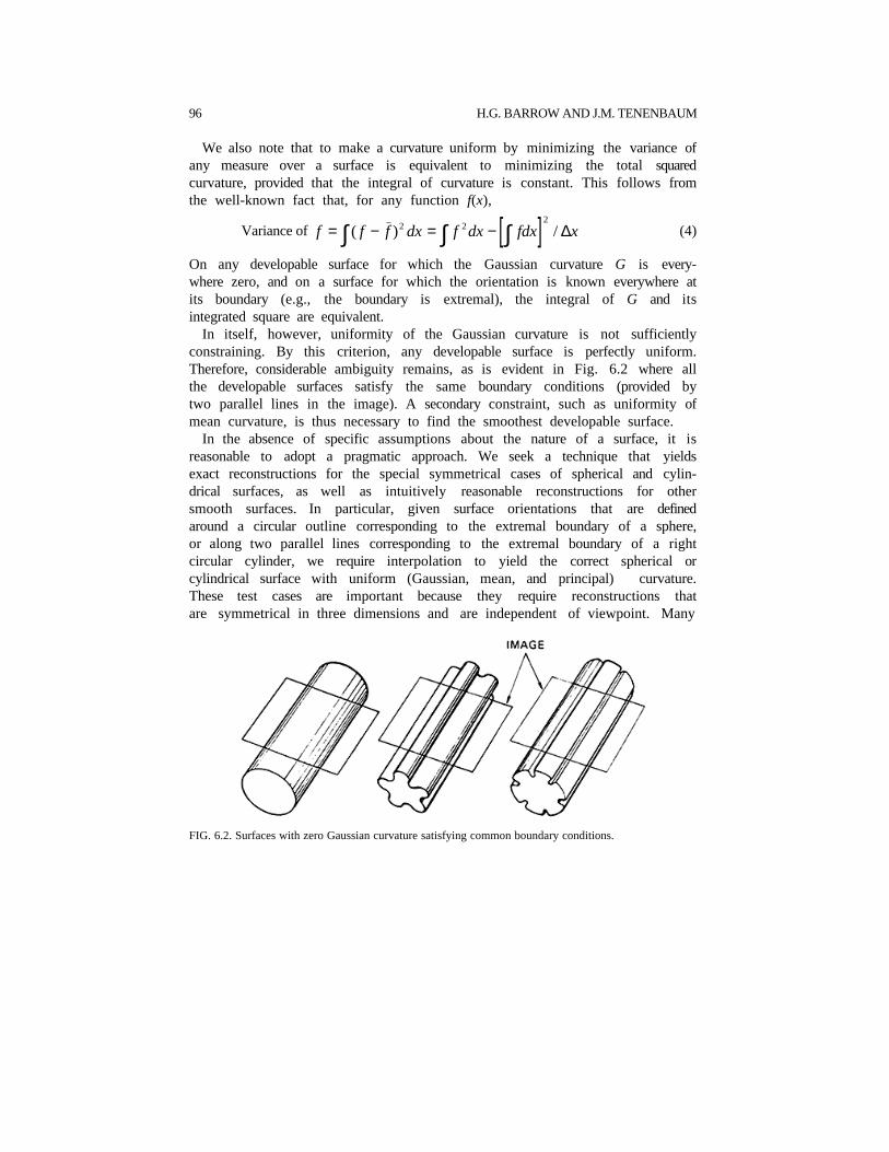
In itself, however, uniformity of the Gaussian curvature is not sufficientlyconstraining. By this criterion, any developable surface is perfectly uniform. Therefore, considerable ambiguity remains, as is evident in Fig. 6.2 where all the developable surfaces satisfy the same boundary conditions (provided by two parallel lines in the image). A secondary constraint, such as uniformity of mean curvature, is thus necessary to find the smoothest developable surface.
In the absence of specific assumptions about the nature of a surface, it is reasonable to adopt a pragmatic approach. We seek a technique that yields exact reconstructions for the special symmetrical cases of spherical and cylin- drical surfaces, as well as intuitively reasonable reconstructions for other smooth surfaces. In particular, given surface orientations that are defined around a circular outline corresponding to the extremal boundary of a sphere, or along two parallel lines corresponding to the extremal boundary of a right circular cylinder, we require interpolation to yield the correct spherical or cylindrical surface with uniform (Gaussian, mean, and principal) curvature. These test cases are important because they require reconstructions that are symmetrical in three dimensions and are independent of viewpoint. Many
FIG. 6.2. Surfaces with zero Gaussian curvature satisfying common boundary conditions.

INTERPRETING LINE DRAWINGS 97
FIG. 6.3. Coordinate frame.
simple interpolation techniques fail this test, producing surfaces that are too flat or too peaked. If we get good performance on the test cases, we can expectreasonable performance in general.
6.2. A reconstruction algorithm
Although in principle correct reconstruction for our test cases can be obtained in many ways, the complexity and generality of the interpolation process depends critically upon the representation employed. For example, represent- ing surface orientation in terms of gradient space leads to difficulties, because gradient variation is extremely nonlinear across the image of a smooth surface,becoming infinite at extremal boundaries. We shall now propose an approach that results in elegantly simple interpolation for our test cases.
6.2.1. Coordinate frames
Given an image plane, we shall assume a right-handed Cartesian coordinate system with x- and y-axes lying in the plane (see Fig. 6.3). We also assumeorthogonal projection in the direction of the z-axis. Each image point (x, y) has an associated range, Z(x, y); the corresponding scene point is thus specified by (x, y, Z(x, y)).
Each image point also has an associated unit vector that specifies the local surface orientation at the corresponding scene point:
N(x, y) = (Nx(x, y), Ny(x, y), Nz(x, y))
Since N is normal to the surface Z,
Nx/Nz = -∂Z/∂x and Ny/Nz = -∂Z/∂y. (5)
(The derivatives ∂Z/∂x and ∂Z/∂y correspond to p and q when the surface normal is represented in gradient space form (p, q, -1).)

98 H.G. BARROW AND J.M. TENENBAUM
Differentiating (5), we obtain
∂(Nx/Nz)/∂y = -∂2Z/∂y ⋅ ∂x
and (6)
∂(Ny/Nz)/∂x = -∂2Z/∂x ⋅ ∂y.
For a smooth surface, the terms on the right of (6) are equal; hence
∂(Nx/Nz)/∂y = ∂(Ny/Nz)/∂x. (7)
Finally, since N is a unit vector,
N N Nx y z2 2 2 1+ + = . (8)
6.2.2. Semicircle
Let us begin by considering a two-dimensional version of surface recon- struction. In Fig. 6.4 we observe that the unit normal to a semicircular surface cross section is everywhere aligned with the radius. It therefore follows that triangles OPQ and PST are similar, and so
OP : OQ : QP = PS : PT : TS. (9)
But the vector OP is the radius vector (x, z), and PS is the unit normal vector (Nx, Nz). Moreover, the length OP is constant (equal to R), and the length PS is also constant (equal to unity). Hence
Nx = x/R and Nz = z/R . (10)
FIG. 6.4. Linear variation of N on a semicircle.
6.2.3. Sphere
Now consider a three-dimensional spherical surface, as shown in Fig. 6.5. Here too the radius and normal vectors are aligned, and so from similar figures we have
Nx = x/R , Ny = y/R and Nz = z/R . (11)
It should be noted that Nx and Ny are both linear functions of x unit length.

INTERPRETING LINE DRAWINGS 99
FIG. 6.5. Linear variation of N on a sphere.
6.2.4. Cylinder
The case of the right circular cylinder is only a little more complicated. In Fig. 6.6 observe a cylinder of radius R centered upon a line in the x-y plane, inclined at an angle A to the x axis. Let d be the distance of point (x, y, 0) from the axis of the cylinder. Then
d = y ⋅ cosA - x ⋅ sin A (12)
and
z2 = R 2 - d2. (13)
Let Nd be the component of vector N parallel to the x-y plane: it is clearly
FIG. 6.6. Linear variation of N on a cylinder.

100 H.G. BARROW AND J.M. TENENBAUM
perpendicular to the axis of the cylinder. Now, since a cross section of the cylinder is analogous to our first, two-dimensional case,
N d = d/R . (14)
Taking components of Nd parallel to the x and y axes:
Nz = Nd ⋅ sin A and Ny = -Nd ⋅ cos A . (15)
Substituting in this equation for Nd and then for d, yields
Nx = ((y cos A - x sin A) ⋅ sin A)/R
and (16)
Ny = (-(y ⋅ cos A - x ⋅ sin A) ⋅ cos A)/R.
Observe that, as was true for the sphere, Nr and Ny are linear functions of x and y, and that Nz can be derived from Nx and Ny.
6.3. A computational model for surface reconstruction
Because of the global nature of the linearity of Nx and Ny for spherical and cylindrical surfaces, it is possible to interpolate the normal vector everywhere in the image from known values at any three noncollinear points. Moreover, Nx and Ny can be treated as independent variables, and yet the vector field produced is guaranteed to satisfy the integrability constraint of (7). This may beverified by substituting for Nx, Ny, and Nz from (11) or (16) (for the sphere or cylinder, respectively) and (8). Hence, the orientation field can be integrated to recover range values.
For arbitrary surfaces, approximated locally by spherical or cylindrical pat- ches, Nx and Ny may be regarded as linear locally, but not globally. The interpolation scheme, therefore, must also be local in nature. While in principle the integrability constraint should not be ignored, in actual practice it is weak; Nx and Ny can be interpolated independently without introducing significant errors.
We have implemented a recovery model that exploits these notions of local linearity and separability to reconstruct arbitrary smooth surfaces. The overall system organization is a subset of the array stack architecture first proposed in [4]. In concept it consists of two primary arrays: one for range and the other for surface normal vectors. The arrays are in registration with each other and with the input image. Values at each point within an array are constrained by local processes that maintain smoothness, as well as by processes that operate between arrays to maintain the differential/integral relationship. The system is designed to be initialized with orientation values and constraints derived from the preceding boundary interpretation stage. (Partially constrained orientations along discontinuity boundaries, however, have not yet been implemented.)
INTERPRETING LINE DRAWINGS 101
6.4. The interpolation process
At each point in the orientation array we can imagine a process that is attempting to make the two observable components of the normal, Nx and Ny, each vary as linearly as possible in both x and y. The process looks at the values of Nx (or Ny) in a small patch surrounding the point, and attempts to infer the linear function, f = ax + by + c, that best models Nx locally. It then tries to relax the value for the point so as to reduce the supposed error.
There are numerous ways to implement such a process, and we shall describe some with which we have experimented. One of the simplest is to perform a local least-squares fit, deriving the three parameters a, b, and c. The function f is then used to estimate a corrected value for the central point. The least- squares fitting process is equivalent to taking weighted averages of the values in the patch, using three different sets of weights:
x Ni xii
⋅∑ , y Ni xii
⋅∑ , Nxii
∑ . (17)
The three parameters of f are given by three linear combinations of these three averages.
If we are careful to use a symmetrical patch with its origin at the point in question, the sets of weights and the linear combinations are particularly simple–the three sums in (17) correspond, respectively, to
a xii
⋅ ∑ 2 , b yii
⋅∑ 2 , ci
⋅ ∑1. (18)
Equations (17) and (18) can be readily solved for a, b, and c; but note that under the above assumptions f(0, 0) = c, so that computation of a and b is unnecessary for updating the central point, unless derivatives are also of interest.
An alternative approach to interpolation follows from the fact that a linear function satisfies the equation
∇ 2f = 0. (l9)
The numerical solution of this equation, subject to boundary conditions, is well known. The ∇ 2 operator may be discretely approximated by the operator
-1-1 4 -1 . -1
Applying this operator at a point in the image leads to an equation of the form
4Nx0 = Nx1 - Nx2 - Nx3 - Nx4 = 0, (20)

102 H.G. BARROW AND J.M. TENENBAUM
and hence, rewriting,
Nxo = (Nx1 + Nx2 + Nx3 + Nx4)/4 . (21)
Equation (21) is used in a relaxation process that iteratively replaces the value of Nx0 at each point with the average of its neighbors. Although the underlying theory is different from least-squares fitting, the two methods lead to essentially the same discrete numerical implementation.
The iterative local-averaging approach works well in the interior regions of asurface, but difficulties arise near surface boundaries where orientation is permitted to be discontinuous. Care must be taken to ensure that the patch under consideration does not fall across the boundary, otherwise estimation of the parameters will be in error. On the other hand, it is necessary to be able to estimate values right up to the boundary, which, for example, may result fromocclusion by another surface.
The least-squares method is applicable to any shape of patch which we can simply truncate at the boundary. However, the linear combination used to compute each parameter depends upon the particular shape, so we must eitherprecompute the coefficients for all possible patches (256 for a 3 X 3 area) or resort to inverting a 3 X 3 matrix to derive them for each particular patch. Neither of these alternatives is attractive, although we might consider pre- computing coefficients for the more common patch shapes, and deriving them when needed for the less common ones.
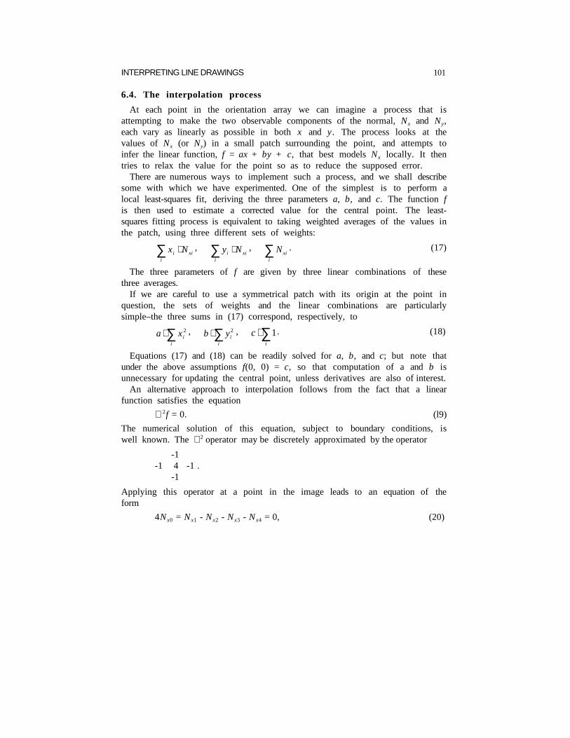
The above disadvantages can be overcome by decomposing the two-dimen- sional fitting process into several one-dimensional fits. We do this by consider- ing a set of line segments passing through the central point, as shown in Fig. 6.7. Along each line we fit a function, f = ax + c, to the data values and thus establish a corrected value for the point. The independent estimates produced from the set of line segments can then be averaged. If the line segments are each symmetrical about the central point, then the corrected central value is here too simply the average of the values along the line The principal advantage of the decomposition is that we can discard line segments that overlap a boundary; often at least one is left to provide a corrected value. We would prefer to use short symmetrical line segments, since they form a compact
FIG. 6 7. Symmetric linear interpolation operators.
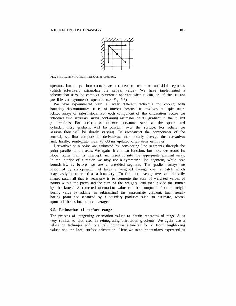
INTERPRETING LINE DRAWINGS 103
FIG. 6.8. Asymmetric linear interpolation operators.
operator, but to get into corners we also need to resort to one-sided segments (which effectively extrapolate the central value). We have implemented a scheme that uses the compact symmetric operator when it can, or, if this is notpossible an asymmetric operator (see Fig. 6.8).
We have experimented with a rather different technique for coping with boundary discontinuities. It is of interest because it involves multiple inter- related arrays of information. For each component of the orientation vector weintroduce two auxiliary arrays containing estimates of its gradient in the x and y directions. For surfaces of uniform curvature, such as the sphere and cylinder, these gradients will be constant over the surface. For others we assume they will be slowly varying. To reconstruct the components of the normal, we first compute its derivatives, then locally average the derivatives and, finally, reintegrate them to obtain updated orientation estimates.
Derivatives at a point are estimated by considering line segments through the point parallel to the axes. We again fit a linear function, but now we record its slope, rather than its intercept, and insert it into the appropriate gradient array. In the interior of a region we may use a symmetric line segment, while nearboundaries, as before, we use a one-sided segment. The gradient arrays are smoothed by an operator that takes a weighted average over a patch which may easily be truncated at a boundary. (To form the average over an arbitrarily shaped patch all that is necessary is to compute the sum of weighted values of points within the patch and the sum of the weights, and then divide the former by the latter.) A corrected orientation value can be computed from a neigh- boring value by adding (or subtracting) the appropriate gradient. Each neigh- boring point not separated by a boundary produces such an estimate, where- upon all the estimates are averaged.
6.5. Estimation of surface range
The process of integrating orientation values to obtain estimates of range Z is very similar to that used in reintegrating orientation gradients. We again use arelaxation technique and iteratively compute estimates for Z from neighboring values and the local surface orientation. Here we need orientations expressed as
104 H.G. BARROW AND J.M. TENENBAUM
∂Z/∂x and ∂Z/∂y, which are obtained from Nx and Ny by (5). At least one absolute value of Z must be furnished to serve as a constant of integration. Providing more than one initial Z value constrains the surface to pass through the specified points. However, since the inverse path from Z to N has not yet been implemented, the resulting range surface is not guaranteed to be con- sistent with the orientations.
6.6. Experimental results
An interactive system was implemented in MAINSAlL [22] to experiment with and to evaluate the various interpolation algorithms discussed above. This system includes facilities for generating quadric surface test cases, selectinginterpolation options, and plotting error distributions.
6.6.1. Test cases
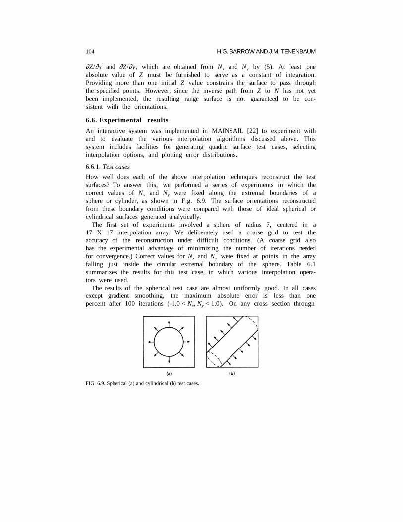
How well does each of the above interpolation techniques reconstruct the test surfaces? To answer this, we performed a series of experiments in which the correct values of Nx and Ny were fixed along the extremal boundaries of a sphere or cylinder, as shown in Fig. 6.9. The surface orientations reconstructed from these boundary conditions were compared with those of ideal spherical orcylindrical surfaces generated analytically.
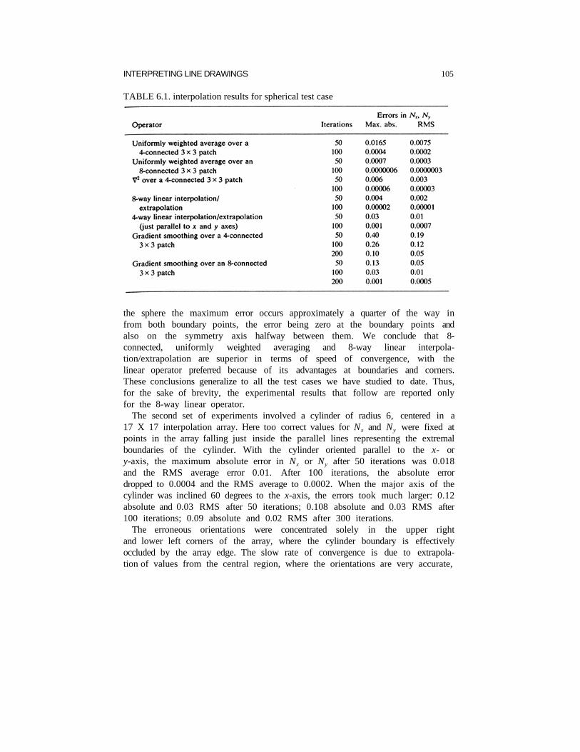
The first set of experiments involved a sphere of radius 7, centered in a 17 X 17 interpolation array. We deliberately used a coarse grid to test the accuracy of the reconstruction under difficult conditions. (A coarse grid also has the experimental advantage of minimizing the number of iterations needed for convergence.) Correct values for Nx and Ny were fixed at points in the array falling just inside the circular extremal boundary of the sphere. Table 6.1 summarizes the results for this test case, in which various interpolation opera- tors were used.
The results of the spherical test case are almost uniformly good. In all cases except gradient smoothing, the maximum absolute error is less than one percent after 100 iterations (-1.0 < Nx, Ny < 1.0). On any cross section through
FIG. 6.9. Spherical (a) and cylindrical (b) test cases.
INTERPRETING LINE DRAWINGS 105
TABLE 6.1. interpolation results for spherical test case
the sphere the maximum error occurs approximately a quarter of the way in from both boundary points, the error being zero at the boundary points and also on the symmetry axis halfway between them. We conclude that 8- connected, uniformly weighted averaging and 8-way linear interpola- tion/extrapolation are superior in terms of speed of convergence, with the linear operator preferred because of its advantages at boundaries and corners. These conclusions generalize to all the test cases we have studied to date. Thus, for the sake of brevity, the experimental results that follow are reported only for the 8-way linear operator.
The second set of experiments involved a cylinder of radius 6, centered in a 17 X 17 interpolation array. Here too correct values for Nx and Ny were fixed at points in the array falling just inside the parallel lines representing the extremalboundaries of the cylinder. With the cylinder oriented parallel to the x- or y-axis, the maximum absolute error in Nx or Ny after 50 iterations was 0.018 and the RMS average error 0.01. After 100 iterations, the absolute error dropped to 0.0004 and the RMS average to 0.0002. When the major axis of thecylinder was inclined 60 degrees to the x-axis, the errors took much larger: 0.12absolute and 0.03 RMS after 50 iterations; 0.108 absolute and 0.03 RMS after 100 iterations; 0.09 absolute and 0.02 RMS after 300 iterations.
The erroneous orientations were concentrated solely in the upper right and lower left corners of the array, where the cylinder boundary is effectively occluded by the array edge. The slow rate of convergence is due to extrapola- tion of values from the central region, where the orientations are very accurate,
106 H.G. BARROW AND J. M. TENENBAUM
into these partially occluded corners. After 1000 iterations, however, orien- tations are highly accurate throughout the array.
6.6.2. Other smooth surfaces
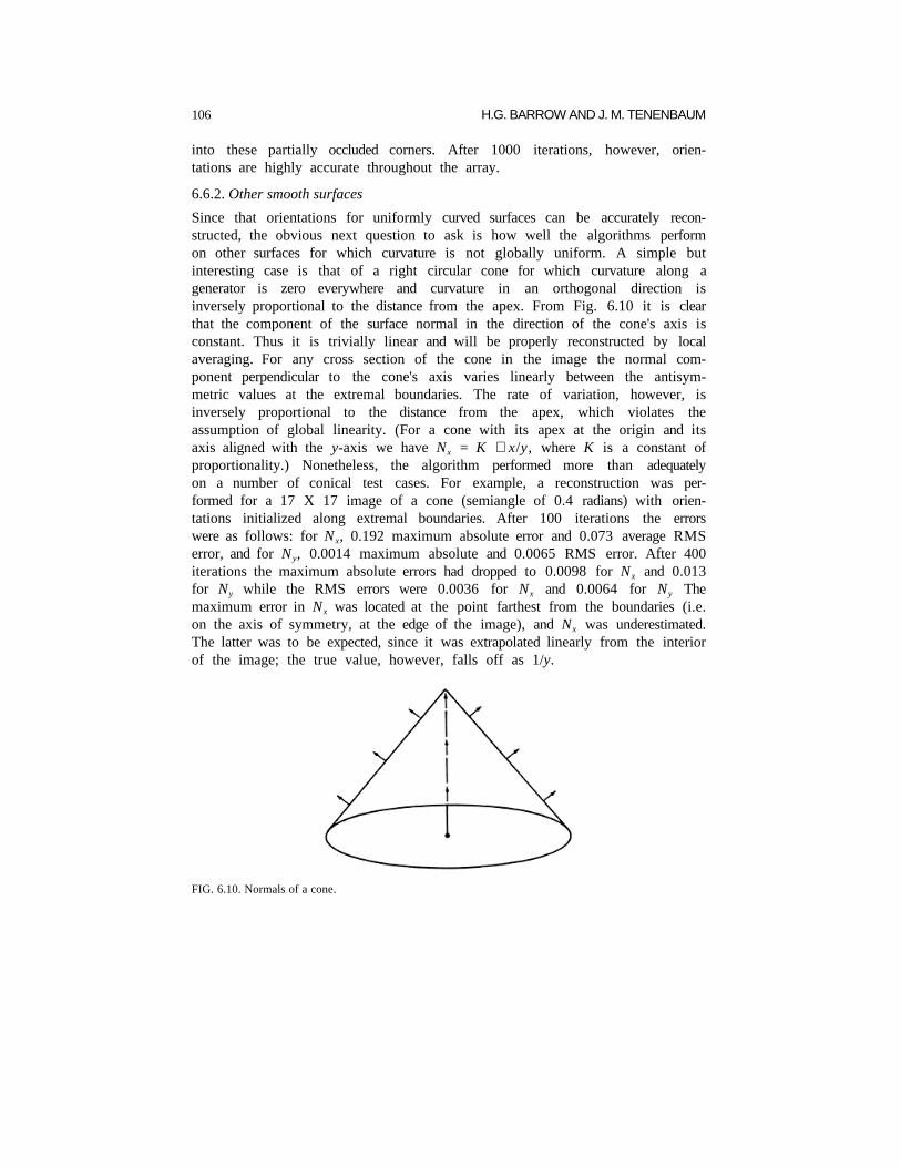
Since that orientations for uniformly curved surfaces can be accurately recon- structed, the obvious next question to ask is how well the algorithms perform on other surfaces for which curvature is not globally uniform. A simple but interesting case is that of a right circular cone for which curvature along a generator is zero everywhere and curvature in an orthogonal direction is inversely proportional to the distance from the apex. From Fig. 6.10 it is clear that the component of the surface normal in the direction of the cone's axis is constant. Thus it is trivially linear and will be properly reconstructed by localaveraging. For any cross section of the cone in the image the normal com- ponent perpendicular to the cone's axis varies linearly between the antisym- metric values at the extremal boundaries. The rate of variation, however, is inversely proportional to the distance from the apex, which violates the assumption of global linearity. (For a cone with its apex at the origin and its axis aligned with the y-axis we have Nx = K ⋅ x/y, where K is a constant ofproportionality.) Nonetheless, the algorithm performed more than adequately on a number of conical test cases. For example, a reconstruction was per- formed for a 17 X 17 image of a cone (semiangle of 0.4 radians) with orien- tations initialized along extremal boundaries. After 100 iterations the errors were as follows: for Nx, 0.192 maximum absolute error and 0.073 average RMS error, and for Ny, 0.0014 maximum absolute and 0.0065 RMS error. After 400iterations the maximum absolute errors had dropped to 0.0098 for Nx and 0.013 for Ny while the RMS errors were 0.0036 for Nx and 0.0064 for Ny The maximum error in Nx was located at the point farthest from the boundaries (i.e. on the axis of symmetry, at the edge of the image), and Nx was underestimated. The latter was to be expected, since it was extrapolated linearly from the interior of the image; the true value, however, falls off as 1/y.
FIG. 6.10. Normals of a cone.

INTERPRETING LINE DRAWINGS 107
The results for cones should extend to generalized cylinders, which have a circular cross-section whose radius varies along a well-defined axis. Such bodiescomprise a broad range of common shapes, from anatomical components (limbs, trunk) to household items, such as the vases in Fig. 6.11. Where the radius of the cross section is locally constant the surface approximates a cylinder and will be reconstructed fairly accurately; where the variation in radius is roughly linear the surface is approximately conical and, as we have seen, will be treated reasonably.
Any inaccuracies in reconstructing cones and generalized cylinders arise because the interpolation is two-dimensional. A one-dimensional algorithm,interpolating perpendicularly to the symmetry axis, would reconstruct the circular cross sections of these objects exactly. While one-dimensional inter- polation is simpler, it requires the additional step of first determining the symmetry axis. A simple experiment suggests that people perform two-dimen- sional interpolation, despite their well-known ability to determine axes of symmetry. The two vases of Fig. 6.11 have generators of the same shape, but differing radii. For the broader vase the perceived variation of depth along the axis of symmetry is less pronounced than it would be if reconstruction were perfect. One explanation is that the reconstruction is two-dimensional, which tends to smooth the surface far from the boundaries, rather than one-dimen- sional, which produces accurate cross sections. There may, of course, be otherexplanations. It is interesting to note that, if the broad vase is interpreted as arectangular sheet undulating in depth, rather than a solid of revolution, the perceived variation of depth along the symmetry axis becomes much more pronounced.
Another interesting case to consider is interpretation of the surface defined by an elliptical boundary. In this case, however, we immediately run into the problem of what is to be taken as the ‘correct’ reconstruction. When people are asked what solid surface they perceive, they usually report either an elongated or squat object, roughly corresponding to a solid of revolution about the major or minor axis, respectively. The elongated object is preferred, and one can argue
FIG. 6.11. The same generator, but different perceived surfaces.

108 H.G. BARROW AND J.M. TENENBAUM
FIG. 6.12. Elliptical test case.
that it is more plausible on the grounds of general viewpoint (a fat, squat object looks elongated only from a narrow range of viewpoints). When presented with initial orientations for an elliptical extremal boundary (Fig 6.12), our algorithms reconstruct an elongated object with approximately uniform curvature about the major axis. In effect, they reconstruct a general- ized cylinder [16], but without explicitly invoking processes to find the axis ofsymmetry or matching the opposite boundaries.
In a representative experiment, initial values for Nx and Ny were fixed inside an elliptic extremal boundary (major axis 15, minor axis 5). The reconstructedorientations were then compared with the orientations of the solid of rev- olution, generated when the ellipse was rotated about its major axis. The resulting errors after 50 iterations were as follows: for Nx, 0.02 maximum 3 absolute error and 0.006 average RMS error; for Ny, 0.005 maximum absolute and 0.002 RMS.
6.6.3. Occluding boundaries
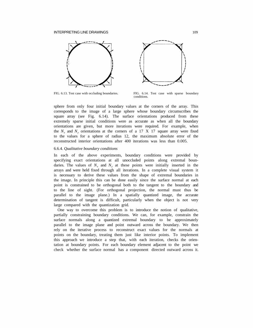
We also wish to know how well the reconstruction process performs when theorientation is not known at all boundary points. In particular, when the surface of interest is occluded by another object, the occluding boundary imposes noconstraints. In such cases the orientation at the boundary must be inferred from that of neighboring points, just as at any other interior point of the surface. The 8-way linear operator will handle these situations correctly, since it is careful to avoid interpolating across boundaries. We take advantage of thiscapability by treating the borders of the orientation array as occluding boun- daries, so that we may deal with objects that extend beyond the image. For example, spherical surface orientations were correctly recovered from the partially visible boundary shown in Fig. 6.13. The case of the tilted cylinder discussed above is a second example.
Experiments with occluded boundaries raised the question of just how little boundary information suffices to effect recovery. We experimented with a limiting case in which we attempted to reconstruct surface orientation of a
INTERPRETING LINE DRAWINGS 109
FIG. 6.13. Test case with occluding boundaries. FIG. 6.14. Test case with sparse boundaryconditions.
sphere from only four initial boundary values at the corners of the array. Thiscorresponds to the image of a large sphere whose boundary circumscribes the square array (see Fig. 6.14). The surface orientations produced from these extremely sparse initial conditions were as accurate as when all the boundaryorientations are given, but more iterations were required. For example, when the Nx and Ny orientations at the corners of a 17 X 17 square array were fixed to the values for a sphere of radius 12, the maximum absolute error of the reconstructed interior orientations after 400 iterations was less than 0.005.
6.6.4. Qualitative boundary conditions
In each of the above experiments, boundary conditions were provided by specifying exact orientations at all unoccluded points along extremal boun- daries. The values of Nx and Ny at these points were initially inserted in the arrays and were held fixed through all iterations. In a complete visual system it is necessary to derive these values from the shape of extremal boundaries in the image. In principle this can be done easily since the surface normal at each point is constrained to be orthogonal both to the tangent to the boundary and to the line of sight. (For orthogonal projection, the normal must thus be parallel to the image plane.) In a spatially quantized image, the accurate determination of tangent is difficult, particularly when the object is not very large compared with the quantization grid.
One way to overcome this problem is to introduce the notion of qualitative, partially constraining boundary conditions. We can, for example, constrain the surface normals along a quantized extremal boundary to be approximately parallel to the image plane and point outward across the boundary. We then rely on the iterative process to reconstruct exact values for the normals at points on the boundary, treating them just like interior points. To implement this approach we introduce a step that, with each iteration, checks the orien- tation at boundary points. For each boundary element adjacent to the point we check whether the surface normal has a component directed outward across it.

110 H.G. BARROW AND J.M. TENENBAUM
If it does not, the value of Nx and Ny is modified appropriately. The value of Nz is also checked to be close to zero, and vector N is normalized to ensure that it remains a unit vector. This process was applied to the spherical, cylindrical, andelliptical test cases; after only 100 iterations it was found to yield orientation values accurate to within ten percent for both interior and boundary points. The principal limitation on accuracy appears to be the coarse quantization grid being used.
7. Discussion
7.1. Summary
We have made a start toward a computational model for interpreting line drawings as three-dimensional surfaces. In the first section we proposed a three-step model for interpretation, based on constraints on local surface orientation along extremal and discontinuity boundaries. We then described specific computational approaches for two key processes: recovering the three-dimensional conformation of a space curve (e.g., a surface boundary) from its two-dimensional projection in an image, and interpolating smooth surfaces from orientation constraints along extremal boundaries.
Some important unresolved problems remain. Our technique for interpreting a three-dimensional space curve is slow and ineffectual on noisy image curves.Furthermore, the surface interpolation technique must be extended to handle partially constrained orientations along discontinuity boundaries.
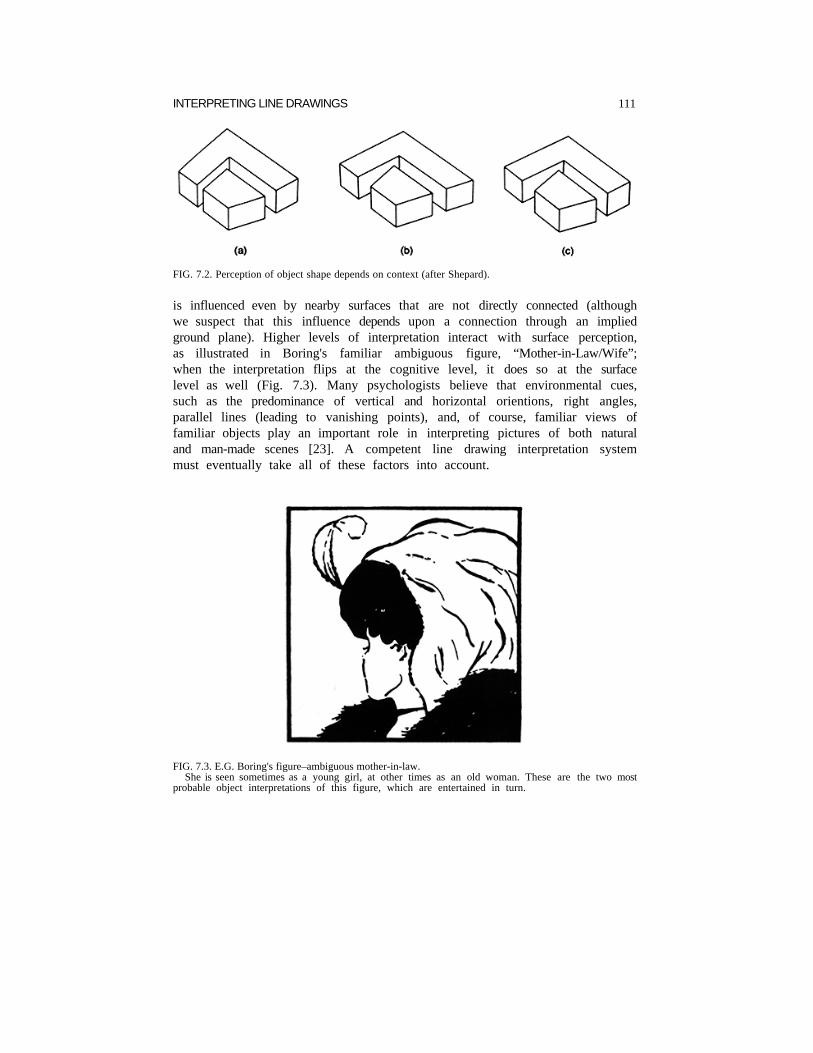
Aspects of line-drawing understanding not yet considered include the effects of context and high-level knowledge. As Fig. 7.1 illustrates, theinterpretation of a surface depends strongly on the perception of adjoining surfaces. Thus, the top surface of the object in Fig. 7.1a appears to undulate in height, while the identically drawn top surface of the object in Fig. 7.1b appears to undulate in depth. Moreover, as suggested in Fig. 7.2, interpretation
FIG. 7.1. Perception of surface shape depends upon adjoining surfaces (after Yonas).(a) Top surface appears to undulate in height.(b) Top surface appears to undulate in depth.
INTERPRETING LINE DRAWINGS 111
FIG. 7.2. Perception of object shape depends on context (after Shepard).
is influenced even by nearby surfaces that are not directly connected (although we suspect that this influence depends upon a connection through an implied ground plane). Higher levels of interpretation interact with surface perception, as illustrated in Boring's familiar ambiguous figure, “Mother-in-Law/Wife”; when the interpretation flips at the cognitive level, it does so at the surface level as well (Fig. 7.3). Many psychologists believe that environmental cues, such as the predominance of vertical and horizontal orientions, right angles, parallel lines (leading to vanishing points), and, of course, familiar views of familiar objects play an important role in interpreting pictures of both natural and man-made scenes [23]. A competent line drawing interpretation system must eventually take all of these factors into account.
FIG. 7.3. E.G. Boring's figure–ambiguous mother-in-law.She is seen sometimes as a young girl, at other times as an old woman. These are the two most
probable object interpretations of this figure, which are entertained in turn.

112 H.G. BARROW AND J.M TENENBAUM
7.2. Relevance to machine vision research
Our interest in line drawings is motivated principally by their possible role in a general theory of low-level vision, specifically their potential for explaining surface perception in regions where photometry is uninformative or too com- plex to model analytically. Line drawings are, however, an extreme abstraction of gray-level imagery, containing no photometric variation. As every artist knows, qualitative shading gradients can be extremely helpful–for example inemphasizing surface relief. It is thus relevant to inquire how photometric information can be used qualitatively in interpreting a gray-level image.
Photometric information is initially used to extract a line drawing from the image. The two major steps in extraction are the detection of intensity discontinuities and the discrimination of those discontinuities that correspond to significant surface discontinuities.
While it is naive to expect a perfect description of intensity discontinuities from any low-level process, David Marr's recent technique for edge detection appears to perform somewhat better than earlier approaches [24]. Marr sug- gests that edge events correspond to zero crossings in the second derivative of band-passed versions of an image, obtained by convolving the image with Gaussian masks of various sizes. Aside from the physiological justifications thatmotivated Marr, the approach has some very attractive practical consequences: edges are found without arbitrary thresholds, they are guaranteed to form closed contours; both step and gradient edges are detected over a wide range of slopes, independent of orientation; weak edges are detected in noise (because of the use of large mask sizes, the smallest of which covers nearly 1000 pixels); the convolved image can be reconstructed from just zero crossinginformation (which suggests that little information may be lost in a line drawing). Drawings derived from zero crossings, while still far from perfect, should be good enough to at least initialize the recovery process; erroneous fragments can be subsequently refined in the light of three-dimensional inter- pretations [4].
Following detection, intensity discontinuities corresponding to surface dis-continuities must be distinguished from those corresponding to shadows, sur- face markings, and other nonstructural features. Our research on intrinsic images leads us to believe that such discrimination may be possible using local image features that do not involve analytic photometry. Illumination edges (shadows), for example, can be distinguished on the basis of their high contrast(typically greater than 30:1) and textutal continuity across the edge. Reflectance edges (painted surface markings, textures) can be distinguished by equality of the ratios of intensity to the intensity gradient on both sides of the edge, as well as by the continuity of gradient direction across the edge. Gloss, highlights, and other specularities have the properties of light sources and can be distinguished by means of local tests developed by Ullman [25] and Forbus [26]. After illumination, reflectance, and specular edges are eliminated, the re-
INTERPRETING LINE DRAWINGS 113
remaining discontinuities correspond to legitimate surface discontinuities: extremal boundaries, occlusion edges, intersection edges, creases, folds, dents, and so forth.
A natural scene often contains so much surface detail that a line drawing representing all visible edges would be of unmanageable complexity. The crucial question is how to determine which edges represent significant detail for the task in hand, and should therefore be included. This question, faced by every artist in sketching a scene, must also be dealt with by any automatic procedure for line-drawing extraction. While we have no solution to this problem, it would seem reasonable to employ a hierarchy of line drawings– progressing from a crude sketch of major surfaces to the detailed micro- structure of local surface features. The levels at which a given edge should berepresented would seem to be related to the spatial frequency bands of a hierarchical edge detection scheme such as Marr's. The lowest-frequency edges would delimit the larger surfaces, and the resulting reconstruction would correspond to a first-order approximation of them. Evidence from higher- frequency bands corresponding to smaller surface detail could refine this description.
Having established a subset of edges comprising a line drawing at a manageable level of detail, photometric information can be used qualitatively for inferring the physical nature of both boundaries and surfaces.
The reasonable assumption that illumination incident on a surface is locally continuous (e.g., from some unspecified, distant point source) leads to a variety of potentially valuable clues. For example, it implies that shading gradients on Lambertian surfaces are caused predominantly by surface cur- vature and not by a falloff of illumination with distance, that gradient directioncorresponds approximately to the direction of maximum curvature on the surface, and that inflections in gray value often correspond to inflections in surface curvature. At extremal boundaries the gradient normal to the boundary is thus likely to be very high, while at occluding contours the gradient is likely to be high along the boundary in the direction of maximum curvature (Fig. 7.4). At arbitrary points on a surface, intensity gradients and their derivatives in twoorthogonal directions can provide a clue to Gaussian curvature, indicating whether the surface is locally planar, cylindrical, elliptic (e.g., spherical), or hyperbolic (inflexive) [11]. They indicate the presence of a bump or dent on anotherwise smooth surface, as well as the relative height of the anomaly.
Qualitative photometric cues are also valuable on specular surfaces. As Kent Stevens observed [17, Section 3.2.2, p. 143], a localized highlight is indicative of an elliptic surface, while a linearly extended one is indicative of a cylindrical surface. Steven's mathematical results are consistent with psychological findings by J. Beck that the presence or absence of a few highlights profoundly influence a viewer’s perception of a surface as entirely shiny or matte, or as either curved or flat (see Fig. 7.5) [27]. It is almost as if the presence of

114 H.G. BARROW AND J.M. TENENBAUM
FIG. 7.4 Qualitative photometric cues to surface shape and boundary type.
FIG. 7.5. The effect of highlights on surface perception (after Beck).Highlights, or regions of strong specular reflection, on a three-dimensional object such as a vase
help to make the entire surface of the vase appear glossy (left). When the photograph is retouched to remove the highlights, the surface of the vase appears matte (right).

INTERPRETING LINE DRAWINGS 115
highlights serves as a switch for selecting a global interpretation. Here too it issignificant that highlights and gloss contours can be locally distinguished from other image intensity features [25, 26].
The above observations, together with the experimental results documented in Fig. 1.3, lead us to speculate that the primary role of photometric cues in human vision may be in qualitative determination of boundary and surface types, rather than in quantitative determination of shape, as has long been advocated by Horn [13]. If this is true, an analogous case could be made for thequalitative interpretation of texture gradients.
Surface boundaries depicted in line drawings provide a good estimation of surface structure in the absence of other information. In a complete vision system information from contours must be combined with information from many other sources—such as texture gradient, stereopsis, and shading–to recover a more accurate and complete description of surface shape. Since contour, texture, and stereopsis rely on the geometry of intensity dis- continuities, rather than the photometry of shading gradients, they are in- herently easier to model. Moreover, since discontinuities can be classified by using only qualitative photometry, it is easier to decide that a geometric cue isapplicable than to decide that a shading gradient should be attributed to surface curvature (in contrast to, say, an illumination gradient). These thoughts suggest that geometric cues may be primary in early vision, providing an estimate of surface structure that can then be refined, where possible, by exploiting photometric cues, e.g., to detect bumps and dents. Once the surface structure has been recovered, reflectance characteristics can be properly esti- mated by using the techniques of Land [28] and Horn [12]; strictly speaking, these are applicable only over continuous surfaces.
This view that geometric cues may be primary is not necessarily inconsistent with our previous recovery model for intrinsic images [4]; a key concept of which was the simultaneous recovery of all surface attributes. The geometric cues simply provide additional information that can be used to improve the boundary conditions that initialize the recovery process. However, the pos- sibility of an alternative sequential recovery model that recovers surface structure from geometric cues before involving photometric characteristics isintriguing. A critical psychological experiment to determine which model most closely resembles the human visual process would be valuable.
ACKNOWLEDGMENT
This paper was begun at SRI, jointly supported by NSF, DARPA, and NASA, and was completed atFairchild.
Albert Yonas, University of Minnesota, and Andrew Hansen, currently at SRI, participated significantly in the early development of our ideas. Discussions with Richard Gregory, University of Bristol, and Andrew Witkin, MIT (now at SRI), were also valuable.

116 H.G. BARROW AND J.M. TENENBAUM
REFERENCES
1. Horn, B.K.P., Understanding image intensities, Artificial Intelligence 8(2) (1977) 201-231.2. Horn, B.K.P., Determining lightness from an image, Comput. Graphics and Image Processing 3 (1974)
277-299.3. Marr, D., Representing visual information, in: A. Hanson and E.M. Riseman, Eds., Computer Vision
Systems (Academic Press, New York, 1978).4. Barrow, H.G. and Tenenbaum, J.M., Recovering intrinsic scene characteristics from images, in: A.
Hanson and E. Riseman, Eds., Computer Vision Systems (Academic Press, New York, 1978).5. Shepard, R.N.. Psychophysical complementarily, in: M. Kubovy and J.R. Pomeranz, Eds., Perceptual
Organization (Lawrence Erlbaum Ass., Hillsdale, 1979).6. Gregory, R., The Intelligent Eye (McGraw-Hill, New York, 1970).7. Roberts, L.G., Machine perception of three-dimensional solids, in: J.T. Tippett et al., Eds, Optical and
Electro-Optical Information Processing (M.I.T. Press, Cambridge, MA, 1965).8. Falk. G., Interpretation of imperfect line data as a three-dimensional scene, Artificial Intelligence 4(2)
(1972) 101-144.9. Huffman, D.A., Impossible objects as nonsense sentences, in: B. Meltzer and D. Michie, Eds., Machine
Intelligence (Edinburgh University Press, Edinburgh, 1971).10. Waltz, D.L., Generating semantic descriptions from drawings of scenes with shadows, Tech. Rept. AI-
TR-271, M.l.T., Cambridge, MA (1972).11. Turner, K.J., Computer perception of curved objects using a television camera, Ph.D. Dissertation,
Edinburgh University, November 1974.12. Marr, D. and Nishihara, H.K., Representation and recognition of the spatial organization of three-
dimensional shapes, Proc. Roy. Soc. London Ser. B 200 (1977) 269-294.13. Stevens, K.A., Constraints on the visual interpretation of surface contours, AI Memo 522, M.I.T.,
Cambridge, MA (1979).14. Clowes, M.B., On seeing things, Artificial Intelligence 2(1) (1971) 79-ll2.15. Chakravarty, I., A generalized line and junction labeling scheme with applications to scene analysis,
IEEE Trans. Pattern Analysis, Machine Intelligence 1(2) (1979) 202-205.16. Marr, D., Analysis of occluding contour. Proc. Roy. Soc. London Ser. B 197 (1977) 441-475.17. Stevens, K.A., Surface perception from local analysis of texture and contour, Ph.D. Dissertation,
M.l.T.. Cambridge, MA. February 1979.18. Witkin, A.P., The minimum curvature assumption and perceived surface orientation, J. Optical Soc.
Amer. 68 (1978) 1450.19. Brand, L., Vector and Tensor Analysis (Wiley, New York, 1953).20. Almgren, Jr., F.J. and Taylor, J.E., The geometry of soap films and soap bubbles, Sci. Amer. (July
1976) 82-93.21. Huffman, D.A., Curvature and creases: A primer on paper, IEEE Trans. Computers 25(1) (1976).22. Wilcox, C., Dageforde, M. and Jirak, G., MAINSAIL Language Manual, Stanford University, Stanford,
1979.23. Haber, R.N., Perception of visual space in scenes and pictures, Paper presented at Conference on the
Interrelations among the Communicative Senses, Asilomar, CA, September 1978.24. Marr, D. and Hildreth, E., Theory of edge detection. AI Memo 518, M.I.T., Cambridge, MA
(1979).25. Ullman. S., On visual detection of light sources. Biol. Cybernet. 21 (1976) 205-212.26. Forbus, K.D., Light source effects, AI Memo 422, M.I.T., Cambridge, MA (1977).27. Beck. I., Surface Color Perception (Cornell University Press, Ithaca, 1974).28. Land, E.H., The retinex theory of color vision, Sci. Amer. 237(G) (1977) 108-128.29. Binford, T.O., Inferring surfaces from images, Artificial Intelligence 17 (1981) 205-244 [this
volume].
Revised version received October 1980