International Momentum Strategies K. Geert Rouwenhorst ...

Electronic copy available at: http://ssrn.com/abstract=4407

International Momentum Strategies

K. Geert Rouwenhorst*

Yale School of Management135 Prospect Street, New Haven CT 06511, USA

phone: (203) 432 6046email: [email protected]

August 1996Revised: February 1997


Abstract

International equity markets exhibit medium-term return continuation. Between 1980 and 1995 an

internationally diversified portfolio of past medium-term Winners outperforms a portfolio of

medium-term Losers after correcting for risk by more than one percent per month. Return

continuation is present in all twelve sample countries and lasts on average for about one year.

Return continuation is negatively related to firm size, but is not limited to small firms. The

international momentum returns are correlated with the U.S. which suggests that exposure to a

common factor may drive the profitability of momentum strategies.


1

Many papers have documented that average stock returns are related to past performance.

Jegadeesh and Titman (1993) document that over medium-term horizons performance persists:

firms with higher returns over the past three months to one year continue to outperform firms

with low past returns over the same period. By contrast, DeBondt and Thaler (1985,1987)

document return reversals over longer horizons. Firms with poor three- to five-year past

performance earn higher average returns than firms that performed well in the past. There has

been an extensive literature on whether these return patterns reflect an improper response by

markets to information, or that they can be explained by market microstructure biases or by

properly accounting for risk. Fama and French (1996) show that long-term reversals can be1

consistent with a multifactor model of returns, but their model fails to explain medium-term

performance continuation. Chan, Jegadeesh and Lakonishok (1996) find that medium-term return

continuation can in part be explained by underreaction to earnings information, but price

momentum is not subsumed by earnings momentum.

Return reversal and continuation are only two of many patterns that empirical researchers

have uncovered using substantially the same database of U.S. stocks. It can therefore not be ruled

out that these apparent anomalies are simply the outcome of an elaborate data snooping process.

This paper is an attempt to address this concern by studying return patterns in an international

context. While Asness et al. (1996), and Richards (1996) study return patterns across markets at

the country index level, this paper primarily focuses on international return continuation within

markets and across markets at the individual stock level using a sample of 2,190 stocks from 12

European countries from 1978 to 1995. Because of the length of the sample period, the paper2

concentrates only on patterns in medium-term returns. The sample period partly overlaps with the

2

U.S. samples of Jegadeesh and Titman (1993) and Fama and French (1996), and is thus not

strictly independent because of common factors in international markets. However, return

continuation in the U.S. does not seem to be related to common factors or conventional measures

of risk. If return continuation is absent in international markets or, when present, can be

rationalized using conventional measures of risk, this suggests that the U.S. experience may

simply have been unusual. Return continuation which is common to many markets and cannot be

accounted for by risk, points either toward a more serious misspecification of commonly used

asset pricing models or a general tendency of markets to underreact to information.

The main finding of the paper is that an internationally diversified relative strength

portfolio which invests in medium-term Winners and sells past medium-term Losers earns around

1 percent per month. This momentum in returns is not limited to a particular market, but is

present in all 12 markets in the sample. It holds across size deciles, although return continuation is

stronger for small than large firms. The outperformance lasts for about one year, and cannot be

attributed to conventional measures of risk. In fact, controlling for market risk or exposure to a

size factor increases the abnormal performance of relative strength strategies. The paper,

however, presents some evidence that the European and U.S. momentum strategies have a

common component which suggests that exposure to a common factor may drive the profitability

of momentum strategies.

The remainder of the paper is organized as follows. Section I describes the sample and

documents the profitability of medium-term international momentum strategies. Section II shows

that momentum is not restricted to stocks of a particular country or size category. Section III

examines whether the returns to momentum strategies can be explained by conventional asset

3

pricing models. Section IV provides conclusions.

I. Returns of relative strength portfolios.

The sample consists of monthly total returns in local currency for 2,190 firms from 12 European

countries from 1978 through 1995: Austria (60 firms), Belgium (127), Denmark (60), France

(427), Germany(228), Italy (223), The Netherlands (101), Norway (71), Spain (111), Sweden

(134), Switzerland (154) and the United Kingdom (494). The sample covers between 60 and 90

percent of each country’s market capitalization. All returns are converted to Deutschmarks (DM)3

using exchange rate information taken from the Financial Times.

The relative strength portfolios are constructed as in Jegadeesh and Titman (1993). At the

end of each month, all stocks with a return history of at least 12 months are ranked into deciles

based on their past J-month return (J equals 3,6,9, or 12) and assigned to one of ten relative

strength portfolios (1 equals lowest past performance, or “Loser”, 10 equals highest past

performance, or “Winner”). These portfolios are equally weighted at formation, and held for K

subsequent months (K equals 3,6,9, or 12 months) during which time they are not re-balanced.4

The holding period exceeds the interval over which return information is available (monthly),

which creates an overlap in the holding period returns. The paper follows Jegadeesh and Titman

(1993) who report the monthly average return of K strategies, each starting one month apart. This

is equivalent to a composite portfolio in which each month 1/K of the holdings are revised. For

example, towards the end of month t the J=6, K=3 portfolio of Winners consists of three parts: a

position carried over from an investment of one DM at the end of month t-3 in the 10 percent

firms with highest prior six-month performance as of t-3, and two similar positions resulting from

4

a DM invested in the top performing firms at the end of months t-2 and t-1. At the end of month t,

the first of these holdings will be liquidated and replaced with a unit DM investment in the stocks

with highest six-month performance as of time t.

Table I presents the average monthly returns on these composite portfolio strategies

between 1980 and 1995. Panel A shows that an equally-weighted portfolio formed from the5

stocks in the bottom decile of previous three-month performance returns 1.16 percent per month,

0.70 percent less than the top decile portfolio which returns 1.87 percent. For the three-month

holding period (K=3), the excess return from buying Winners and selling Losers increases with

the length of the return interval used for ranking (J). Irrespective of the interval used for ranking,

average returns tend to fall for longer holding periods. For each of the ranking and holding

periods, however, past Winners outperformed past Losers by about 1 percent per month. The

returns range from 0.64 to 1.35 percent per month earned by portfolios based on 12-month

ranked returns held for 12 and three months respectively. All excess returns in Panel A are

significant at the 5 percent level.

The portfolios in Panel A are formed at the end of the performance ranking period.

Because bid-ask bounce can attenuate the continuation effect, Panel B reports the average returns

if the portfolio formation is delayed relative to the ranking by one month. For the shorter ranking

and holding intervals, delaying the portfolio formation indeed increases the payoff to buying

Winners and selling Losers. This increase is primarily due to a lower return to the Loser portfolio.

Bid-ask bounce can also affect the measurement of the holding period returns. Blume and

Stambaugh (1983) have shown that long-term performance measures, obtained by averaging

short-term returns over time, will be biased upward due to measurement error in the returns and

5

bid-ask bounce. This bias affects the apparent profitability of momentum strategies because

Losers are on average smaller than Winners. In addition to the average monthly return on K-6

month strategies given in Table I, I also compute the average K-month holding period returns on

the various strategies, and find the results to be very similar.

The remainder of the paper will concentrate on portfolios formed on the basis of six-

month ranked returns, formed at the end of the ranking period and held for six months. Table II

presents the summary statistics for the 10 decile portfolios of this strategy. The first column

shows that the average performance of the decile portfolios is monotonically increasing in

previous six-month return. Higher past six-month return is on average associated with stronger

future six-month performance. An F-test strongly rejects the equality of average returns of the

relative strength portfolios. The second column of Table II shows that the standard deviation of

the decile portfolios is U-shaped. The Winner and Loser portfolios have standard deviations that

are 30 and 40 percent higher than the portfolios in the middle deciles. All else equal, stocks with

higher standard deviations are more likely to show unusual performance, and past unusual

performance is cross-sectionally correlated with volatility. The standard deviation of the excess

return of Winners over Losers is about 4 percent per month, which is similar to the volatility of a

long position in the middle decile portfolios. This indicates that an “unrestricted” international

momentum portfolio may not be well-diversified. The third columns show that the excess return

of Winners over Losers is unlikely to be explained by their covariances with the market. The

sample average excess return on the market is about 0.6 percent per month. For market risk to

explain a continuation effect of 1.2 percent per month would require, loosely speaking and

ignoring standard errors, that the beta of Winners exceeds the beta of Losers by about two.

6

Instead, both betas with respect to the value-weighted Morgan Stanley Capital International

(MSCI) index are close to unity, and the beta of the excess return of Winners over Losers is

insignificantly different from zero. The last column of Panel A reveals two interesting7

characteristics of the relative strength portfolios. First, the average size of the Losers is smaller

than the average size of the Winners. Although Section III of the paper deals with risk-8

adjustment in more detail, the fact that average returns are negatively related to firm size suggests

that size as a risk factor cannot explain the continuation effect. Second, both Winners and Losers

are on average smaller than the average firm in the sample. This suggests that implementation of

the Winners-Losers (W-L) strategy may be difficult because it predominantly requires positions in

small stocks. The next section shows, however, that this is not the case.

II. Relative strength strategies that control for country and size.

The relative strength portfolios in the previous section combine stocks from 12 national markets,

some of which are larger in size than others. More than half of the 2,190 stocks in the sample are

from the U.K. (494), France (427), or Germany (228). The average market capitalization of these

firms is larger than of firms in the smaller European markets. This raises three questions about the

source and the pervasiveness of the continuation effect. First, the continuation effect may be

confined to only a subset of the twelve markets: either the three largest markets which contribute

the majority of sample firms, or alternatively the smaller European markets which contain

relatively many small and thinly traded issues. Second, no restrictions have been placed on the

geographical composition of the relative strength portfolios and the country weights vary over

time. The continuation effect may therefore in part be due to country momentum. It is interesting

7

therefore to see to what extent the continuation effect holds in individual countries, and is present

in relative strength portfolios that are country-neutral. Finally, because both the Winner and Loser

portfolios in Table II are tilted towards small stocks, I will examine the influence of firm size on

the returns to relative strength strategies. As pointed out before, country membership and firm

size are not independent, and I also present results for portfolios that are both size- and country-

neutral.

A. Relative strength portfolios by country.

Return decompositions by Heston and Rouwenhorst (1994) and Griffin and Karolyi (1996) show

the presence of large country-specific factors in international stock returns. Large country-specific

shocks can potentially lead to poor international diversification of the relative strength portfolios.

For example, a strong performance of German stocks relative to other markets will subsequently

cause the Winner portfolio to be overweighted in Germany relative to the European equally-

weighted index. Similarly, the Loser portfolio will be tilted towards stocks from markets with

poor past performance. One possible explanation for return continuation is that country-specific

market performance persists (Asness et al. (1996) and Richards (1996)). However, if return

continuation is primarily due to country momentum, controlling for the geographical composition

of relative strength portfolios should significantly reduce the average payoffs to buying Winners

and selling Losers. If on the other hand medium-term persistence reflects idiosyncratic firm

performance, return continuation will remain present in country-neutral relative strength

portfolios as well.

Country-neutral relative strength portfolios are formed by ranking stocks into deciles

8

based on past performance relative only to stocks from the same local market. The 10 percent of

stocks from each country with lowest past six-month return are assigned to the Loser portfolio,

the top 10 percent to the Winner portfolio. Except for integer constraints, the resulting decile

portfolios are well-diversified in the sense that they have the same country allocation, and are

country-neutral relative to the equally-weighted index of the twelve countries in the sample. 9

Panel A of Table III shows that controlling for country composition only slightly reduces the

average excess return of Winners over Losers (W-L) from 1.16 to 0.93 percent per month. This

suggests that country momentum is relatively unimportant for explaining the continuation effect.10

The better diversification of the country-neutral relative strength portfolios lowers the standard

deviations of both the Winner and Loser portfolios and increases their correlation from 0.74 to

0.88. As a result, the standard deviation of the excess return falls from 3.97 to 2.39 percent per

month, and the significance of the average excess return increases (t =5.36).

The remainder of Panel A gives the W-L excess returns by country. Winners have

outperformed Losers in all twelve countries. In eleven countries the W-L excess return has a t-

statistic exceeding two, including the largest markets of France, Germany and the United

Kingdom. Only in Sweden is the excess return insignificantly different from zero. The strongest

continuation effect occurred in Spain, followed by The Netherlands, Belgium, and Denmark. The

standard deviations of the individual country excess returns are about two to three times larger

than the standard deviation of the internationally diversified momentum strategy. This implies that

a large portion of the W-L excess return variance is country-specific and can be diversified

internationally. The conclusion from Panel A is that return continuation is not due to country

momentum. It is pervasive, and not restricted to a few individual markets.11

9

B. Size-neutral relative strength strategies.

The unrestricted and country-neutral relative strength strategies in Table II, and Panel A of Table

III are not size-neutral in two respects. First, Loser firms are on average smaller than firms in the

Winner decile. Because Winners are on average larger than Losers, a size effect may attenuate the

Winner-Loser effect. Second, both Winners and Losers are smaller than the average firm in the

sample. This raises the question whether the continuation effect is only limited to smaller stocks.

To control for size I first sort all stocks based on size (market equity), and within each size

decile on past six-month return. The Loser portfolio contains the 10 percent of firms with the

lowest previous performance from each size decile; the firms with the highest past return in each

size decile end up in the Winner portfolio. Both the Winner and the Loser portfolios will therefore

contain the same number of stocks from each size decile, and are in that sense approximately size-

neutral. Panel B of Table III shows that after controlling for size, past Winners significantly

outperform past Losers by 1.17 percent per month (t =4.30). Moreover, return continuation

exists in all size deciles and is not limited to small stocks. However there is a negative relation

between firm size and the excess return of the relative strength portfolios. Winners from the

smallest size decile outperform the Losers on average by 1.45 percent per month, with a standard

deviation of 5.88 percent. The excess return in the largest size decile is on average 0.73 percent

per month with standard deviation of 4.73 percent. The conclusion from Panel B is that the

continuation effect is not merely a reflection of firm size. Although the continuation effect is

stronger for smaller firms, past Winners outperform Losers in every size category.

C. Size/country-neutral relative strength portfolios.

10

Although return continuation is present in many countries and across size deciles, country

membership and size are not independent. The country-specific relative strength portfolios take

significant size bets, while the size-sorted relative strength portfolios take significant country bets.

This section explores the effectiveness of relative strength strategies that avoid taking significant

country and size positions, in order to separate the influence of size and country membership. The

number of sample firms is not sufficient to construct 10 relative strength portfolios for each size

decile in every country, but a coarser sort can provide information about the influence of size

independent of country. Size-country-neutral portfolios are formed by first sorting stocks by

country in three size groups: small (bottom 30%), medium (middle 40%), and large (top 30%).

Within each size-country group, stocks are ranked into deciles based on past six-month

performance. The size-country-neutral Loser (Winner) portfolio contains the stocks from the

lowest (highest) past performance decile from each of the 36 country-size groups. Panel C of

Table III shows that an internationally diversified portfolio of Winners that controls for country

and size has outperformed Losers by 0.85 percent per month (t=5.32). The performance cannot

be attributed to a particular geographical market. The size-neutral W-L excess returns are

significantly different from zero in the three largest markets in the sample (France, Germany, and

the United Kingdom) and comparable to the excess return on a size-neutral W-L portfolio

constructed from stocks from the other 9 markets. Although Winners outperform Losers in each

of the three size categories, the excess return on the country-neutral W-L portfolio of small stocks

is about twice as large as the excess return on the W-L portfolio of large stocks. Interestingly,12

the country-neutral W-L strategy of stocks from the middle 40 percent of the size distribution has

on average earned 0.92 percent per month, which is not significantly different from the 0.85

11

percent earned on the overall size-country-neutral strategy (t =0.91). The overall conclusion is

that while return continuation varies by country and size, profitability of international relative

strength strategies does not require investors to take significant size or country positions.

III. Risk adjusted returns

A. Adjustment for market and size factors.

Panel A of Table IV confirms that the excess return on the unrestricted relative strength strategy

cannot be accounted for by a simple adjustment for beta-risk, because the betas of the Winner and

Loser portfolios are very similar. The alphas of Losers and Winners are �0.27 percent (t =�1.05)

and 0.88 percent (t =4.53) per month respectively, and their difference of 1.14 percent (t =3.94) is

highly significant. Allowing for exposure to size, as measured by an international version of Fama

and French’s (1996) SMB factor, increases the risk adjusted return to 1.46 percent per month

(t=5.05). Similar to the U.S. experience, Losers are on average smaller than Winners and load

more on the international SMB factor. The size-country-neutral W-L portfolio, however, shows13

a similar negative size exposure. Unreported results show that all 10 size-sorted W-L portfolios

summarized in Panel B of Table III have negative loadings on the international SMB portfolio. It

suggests that Losers behave more like small stocks than Winners irrespective of size. The overall

conclusion from Table IV is that a risk adjustment for market and size makes the continuation

effect appear more at odds with the joint hypothesis of market efficiency and the two-factor

model.

Chan (1988) and DeBondt and Thaler (1987) find that abnormal returns associated with

long term return reversal strategies disappear once betas are allowed to vary with market

12

conditions. For the continuation effect to be consistent with market dependent betas requires that

Losers have a higher beta in down markets than Winners, and a lower beta in up markets. Table V

shows that empirically the opposite is true. Although the betas do vary with market conditions,

Losers uniformly have a higher beta in up markets and a lower beta in down markets than

Winners, which makes the alphas appear more anomalous. As a consequence, the beta of the W-L

excess returns are significantly negative in up markets and positive in down markets. The resulting

alphas are 1.41 and 1.99 percent per month respectively for the size-country-neutral and the

unrestricted W-L portfolios.

B. Relative strength strategies in event time.

As noted earlier, the return on the (J,K) relative strength portfolio at time t is determined by the

payoffs to K separate positions put into place at times t-1 through t-K, with each position based

on past J-month performance rankings at those times. In this section I look at the performance of

each of these components in event time: what is the average excess return on buying Winners and

selling Losers (J=6) in the K-th month after the strategy is put into place? This provides

information about the duration of the continuation effect, as well as the extent to which it is

permanent.

Table VI gives the monthly average excess return (W-L) in the first two years after

portfolio formation, both before and after risk adjustment. The raw excess returns are uniformly

positive in the first 11 months after portfolio formation, after which time they turn negative. The

risk-adjusted excess returns are significantly positive in the first 11 months after portfolio

formation. There is some indication of time variation in the risk exposure of the event time

13

portfolios, but it is not sufficient to explain the excess returns. In fact, all event time portfolios

have negative loadings on the SMB factor, which tends to increase the abnormal returns relative

to the raw excess returns. The sample average risk premium of SMB is 0.29 percent per month,

about half the sample average excess return of the market factor which is 0.62 percent per month.

Because the absolute value of the loadings on SMB is more than twice as large as the market

factor loadings, the SMB factor dominates the risk correction of the raw returns. The excess

returns turn negative in the second year after portfolio formation, although the abnormal returns

are never significant. It suggests however, that part of the continuation effect may be temporary

and is reversed in the second year after portfolio formation. These results are strikingly similar to

the results of Jegadeesh and Titman(1993) for the U.S. market. They also report significant raw

excess returns in months two through 10, although the return reversal for the U.S. market in the

second year is somewhat less pronounced than in our European sample.

Figure I presents the evolution of the cumulative payoff to buying Winners and selling

Losers in event time. Both portfolios are size-country-neutral. The solid line is computed as the

average difference between the K-period buy-and-hold returns of the long and short position, and

is free from the potential bias induced by summing short-term returns to obtain long-term

performance measures. The dashed lines mark a 95 percent confidence interval for the average

payoff, using standard errors that take into account the autocorrelation of the payoffs. The size-

country-neutral relative strength strategy has on average a significantly positive payoff up to 24

months after portfolio formation. The payoff initially peaks 12 months after formation at 11.54

Pfennig per DM invested in the long position, after which it stays mostly flat.

Figure I can also be used to assess the profitability of momentum strategy after

14

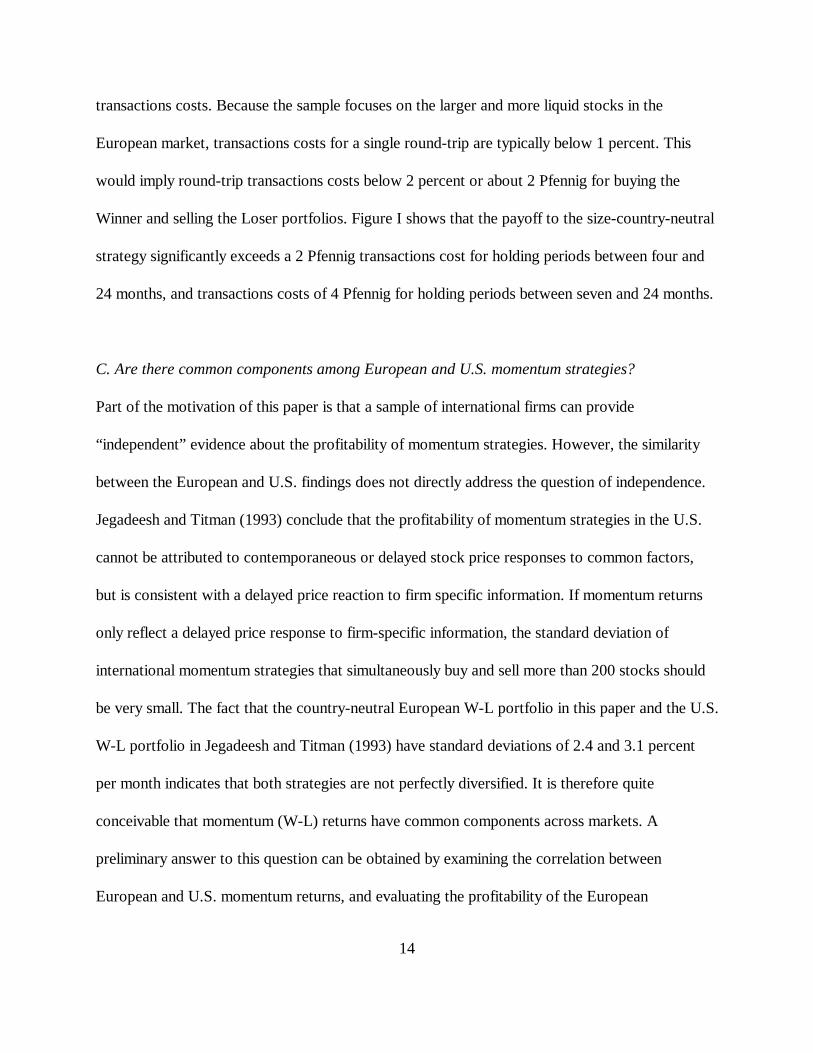
transactions costs. Because the sample focuses on the larger and more liquid stocks in the

European market, transactions costs for a single round-trip are typically below 1 percent. This

would imply round-trip transactions costs below 2 percent or about 2 Pfennig for buying the

Winner and selling the Loser portfolios. Figure I shows that the payoff to the size-country-neutral

strategy significantly exceeds a 2 Pfennig transactions cost for holding periods between four and

24 months, and transactions costs of 4 Pfennig for holding periods between seven and 24 months.

C. Are there common components among European and U.S. momentum strategies?

Part of the motivation of this paper is that a sample of international firms can provide

“independent” evidence about the profitability of momentum strategies. However, the similarity

between the European and U.S. findings does not directly address the question of independence.

Jegadeesh and Titman (1993) conclude that the profitability of momentum strategies in the U.S.

cannot be attributed to contemporaneous or delayed stock price responses to common factors,

but is consistent with a delayed price reaction to firm specific information. If momentum returns

only reflect a delayed price response to firm-specific information, the standard deviation of

international momentum strategies that simultaneously buy and sell more than 200 stocks should

be very small. The fact that the country-neutral European W-L portfolio in this paper and the U.S.

W-L portfolio in Jegadeesh and Titman (1993) have standard deviations of 2.4 and 3.1 percent

per month indicates that both strategies are not perfectly diversified. It is therefore quite

conceivable that momentum (W-L) returns have common components across markets. A

preliminary answer to this question can be obtained by examining the correlation between

European and U.S. momentum returns, and evaluating the profitability of the European

15

momentum strategy conditional on the U.S. experience. The sample correlation between the14

country-neutral European and U.S. momentum returns, cor(W-L , W-L ), is 0.43 over theEUR US

1980 to 1995 period, indicating strong positive dependence across markets. A regression of W-15

L on W-L can be used to evaluate the profitability of the European strategy conditional onEUR US

the U.S. experience:

W-L = 0.0065 + 0.222 W-L + e , R = 0.19,EUR,t US,t t 2

(4.04) (6.62)

where t-statistics are given in parenthesis. Assuming joint normality, the intercept of this

regression measures the average excess return of the component of the European momentum

portfolio which is independent of U.S. momentum returns. Conditioning on the U.S. reduces the

average excess return of the European momentum portfolio from 0.93 (Table III, Panel A) to

0.65 percent per month, but the high t-statistic of the intercept implies profitability of European

momentum strategies that is independent of a common component with the U.S. In this sense the

European sample provides independent evidence of profitability of momentum strategies. While

these results can be consistent with the presence of a “momentum factor” in returns, the

dependence can also be due to non-zero exposures to other common priced risk factors (such as

SMB), common unpriced factors (industry factors), or a combination of both. A more detailed

analysis of this issue is beyond the scope of the current paper, however, and is left for future

research.

IV. Conclusions

16

This paper documents international return continuation in a sample of 12 European countries

during the period 1980 to 1995. An internationally diversified portfolio of past Winners

outperformed a portfolio of past Losers by about 1 percent per month. These relative strength

strategies load negatively on conventional risk factors such as size and the market. The payoffs

are therefore inconsistent with the joint hypotheses of market efficiency and commonly used asset

pricing models. Return continuation is present in all countries, and holds for both large and small

firms, although it is stronger for small firms than large firms. The European evidence is

remarkably similar to findings for the U.S. by Jegadeesh and Titman (1993), and makes it unlikely

that the U.S. experience was simply due to chance. Returns on European momentum portfolios

are significantly correlated with relative strength strategies in the U.S.. Whether this correlation

reflects a priced momentum factor that is common across markets remains a topic for future

research.

17

References

Asness, Clifford, S., 1995, The power of past stock returns to explain future stock returns,

Working paper, Goldman Sachs Asset Management.

Asness, Clifford, S., John M. Liew and Ross L. Stevens, 1996, Parallels between the cross-

sectional predictability of stock returns and country returns, Working paper, Goldman

Sachs Asset Management.

Ball, Ray, and S.P. Kothari, 1989, Nonstationary expected returns: Implications for market

efficiency and serial correlations in returns, Journal of Financial Economics 25, 51-74.

Ball, Ray, S.P. Kothari, and Jay Shanken, 1995, Problems in measuring portfolio performance: An

application to contrarian investment strategies, Journal of Financial Economics 38, 79-

107.

Ball, Ray, S.P. Kothari, and Charles E. Wasley, 1995, Can we implement research on stock

trading rules: the case of short term contrarian strategies, Journal of Portfolio

Management 21, 54-63.

Bekaert, Geert, Claude B. Erb, Campbell R. Harvey, and Tadas E. Viskanta, 1996, The cross-

sectional determinants of emerging equity market returns, Working paper, Duke

University.

Blume, Marshall, and Robert F. Stambaugh, 1983, Biases in computed returns: An application to

the size effect, Journal of Financial Economics 12, 387-404.

Chan, Louis K.C., 1988, On the contrarian investment strategy, Journal of Business 61, 147-163.

Chan, Louis K.C., Yasushi Hamao, and Josef Lakonishok, 1991, Fundamentals and stock returns

in Japan, Journal of Finance 46, 1739-1764.

18

Chan, Louis K.C., Narasimhan Jegadeesh, and Josef Lakonishok, 1996, Momentum Strategies,

Journal of Finance 51, 1681-1713.

Conrad, Jennifer, and Gautam Kaul, 1993, Long-term market overreaction or biases in computed

returns?, Journal of Finance 48, 39-64.

Conrad, Jennifer, and Gautam Kaul, 1996, An anatomy of trading strategies, Working paper,

University of North Carolina.

DeBondt, Werner F.M., and Richard H.Thaler, 1985, Does the stock market overreact?, Journal

of Finance 40, 793-805.

DeBondt, Werner F.M., and Richard H.Thaler, 1987, Further Evidence on investor overreaction

and stock market seasonality, Journal of Finance 42, 557-581.

DeLong, J. Bradford, Andrei Schleifer, Lawrence H. Summers, and Robert J. Waldman, 1990,

Positive feedback investment strategies and destabilizing rational speculation, Journal of

Finance 45, 379-395.

Fama, Eugene F., and Kenneth R. French, 1996, Multifactior explanations of asset pricing

anomalies, Journal of Finance 51, 55-84.

Ferson, Wayne E., and Campbell R. Harvey, 1996, Fundamental determinants of national equity

market returns, NBER Working paper 5860.

Foerster, Stephen, Anoop Prihar, and John Schmitz, 1995, Back to the Future, Canadian

Investment Review 7, 9-13.

Griffin, John M., and G. Andrew Karolyi, 1996, Another look at the role of the industrial

structure of markets for international diversification strategies, Working paper, Ohio State

University.

19

Heston, Steven L., and K. Geert Rouwenhorst, 1994, Does industrial structure explain the

benefits of industrial diversification?, Journal of Financial Economics 36, 3-27.

Jegadeesh, Narasimhan, and Sheridan Titman, 1993, Returns to buying winners and selling losers:

implications for stock market efficiency, Journal of Finance 48, 65-91.

Lakonishok, Josef, Andrei Schleifer, and Robert W. Vishny, 1994, Contrarian investment,

extrapolation and risk, Journal of Finance 49, 1541-1578.

Richards, Anthony J., 1996, Winner-loser reversals in national stock market indices: Can they be

explained?, Journal of Finance, forthcoming.

Table I: Returns of Relative Strength Portfolios

At the end of each month all stocks are ranked in ascending order based on previous J-month performance.The stocks in the bottom decile (lowest previous performance) are assigned to the Loser portfolio, those inthe top decile to the Winner portfolio. The portfolios are initially equally-weighted and held for K months.The table gives the average monthly buy-and-hold returns on these portfolios between 1980 and 1995. InPanel A the portfolios are formed immediately after ranking, in Panel B the portfolio formation occurs onemonth after the ranking takes place.

Panel A Panel B

Holding Period (K) Holding Period (K)RankingPeriod (J) Portfolio 3 6 9 12 3 6 9 12

3 Loser 0.0116 0.0104 0.0108 0.0109 0.0077 0.0087 0.0094 0.0105Winner 0.0187 0.0192 0.0190 0.0191 0.0185 0.0191 0.0190 0.0184

Winner-Loser 0.0070 0.0088 0.0082 0.0082 0.0109 0.0105 0.0095 0.0079(t-stat ) (2.59) (3.86) (4.08) (4.56) (4.29) (4.74) (4.99) (4.64)

6 Loser 0.0095 0.0090 0.0092 0.0104 0.0072 0.0076 0.0088 0.0106Winner 0.0208 0.0206 0.0204 0.0195 0.0204 0.0205 0.0200 0.0187


9 Loser 0.0088 0.0083 0.0097 0.0111 0.0064 0.0077 0.0095 0.0114Winner 0.0212 0.0213 0.0204 0.0193 0.0209 0.0207 0.0197 0.0184


12 Loser 0.0084 0.0094 0.0108 0.0121 0.0077 0.0093 0.0110 0.0125Winner 0.0219 0.0209 0.0197 0.0185 0.0208 0.0198 0.0188 0.0176


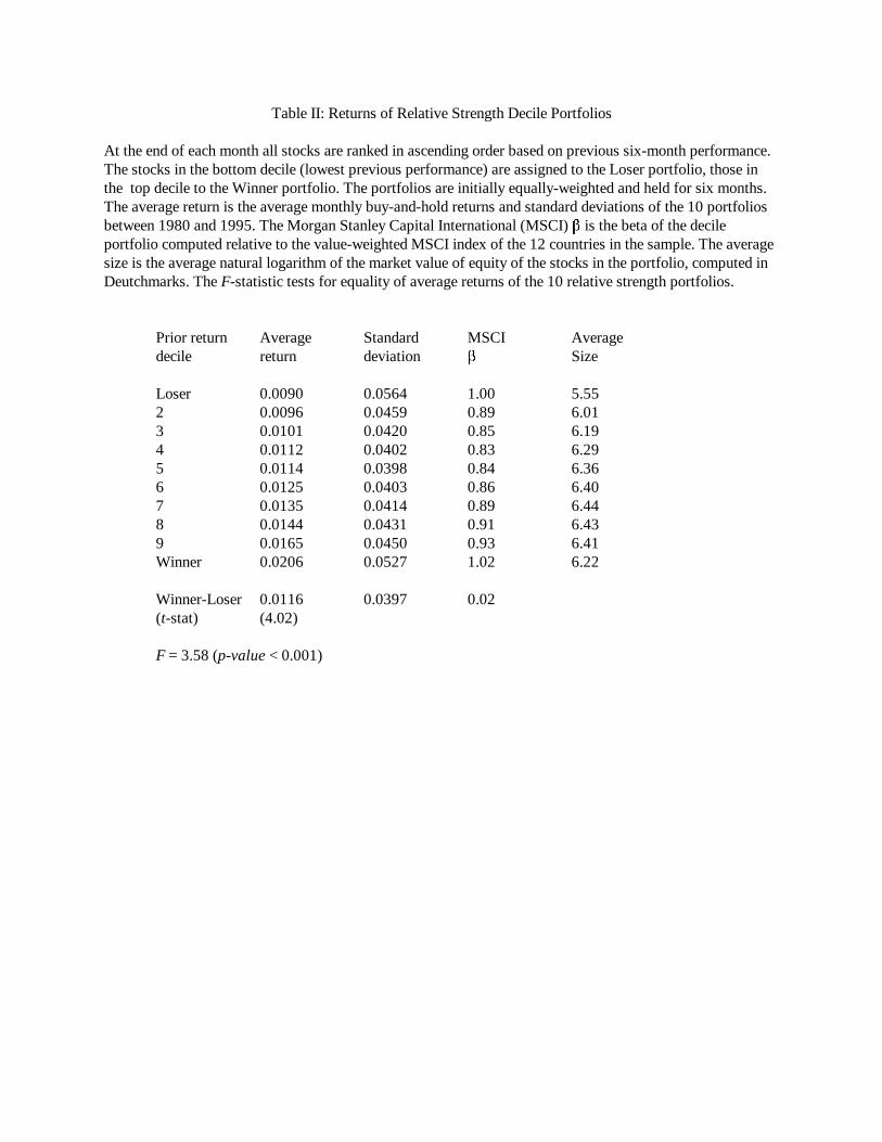
Table II: Returns of Relative Strength Decile Portfolios

At the end of each month all stocks are ranked in ascending order based on previous six-month performance.The stocks in the bottom decile (lowest previous performance) are assigned to the Loser portfolio, those inthe top decile to the Winner portfolio. The portfolios are initially equally-weighted and held for six months.The average return is the average monthly buy-and-hold returns and standard deviations of the 10 portfoliosbetween 1980 and 1995. The Morgan Stanley Capital International (MSCI) � is the beta of the decileportfolio computed relative to the value-weighted MSCI index of the 12 countries in the sample. The averagesize is the average natural logarithm of the market value of equity of the stocks in the portfolio, computed inDeutchmarks. The F-statistic tests for equality of average returns of the 10 relative strength portfolios.

Prior return Average Standard MSCI Averagedecile return deviation � Size

Loser 0.0090 0.0564 1.00 5.552 0.0096 0.0459 0.89 6.013 0.0101 0.0420 0.85 6.194 0.0112 0.0402 0.83 6.295 0.0114 0.0398 0.84 6.366 0.0125 0.0403 0.86 6.407 0.0135 0.0414 0.89 6.448 0.0144 0.0431 0.91 6.439 0.0165 0.0450 0.93 6.41Winner 0.0206 0.0527 1.02 6.22

Winner-Loser 0.0116 0.0397 0.02 (t-stat) (4.02)

F = 3.58 (p-value < 0.001)

Table III: Returns of Relative Strength Portfolios that Control for Country and Size

At the end of each month all stocks are ranked in ascending order based on previous six-month performance,relative to other stocks in its country (Panel A), size decile (Panel B), or size-country group (Panel C). Thebottom decile of stocks are assigned to the Loser (L) portfolio, the top decile to the Winner (W) portfolio.The portfolios are initially equally-weighted and held for six months. Each panel gives the average monthlybuy-and-hold return and standard deviation of an internationally diversified relative strength portfolio and itscomponents between 1980 and 1995. The W-L excess returns for Austria, Denmark, and Norway in panel Aare based on Winner and Loser quintile portfolios due the small number of firms in the sample. The sizeassignments in Panel C correspond to the ranking of stocks in each country on size relative to other stocks inthat country: small (bottom 30%), medium (middle 40%), and large (top 30%). t(mean) is the mean dividedby its standard error.

Panel A: Country-neutral momentum strategies

Portfolio Mean Sdev t(mean)

All stocks (country-neutral) 0.0093 0.0239 5.36

By country:Austria 0.0080 0.0498 2.23Belgium 0.0110 0.0444 3.42Denmark 0.0109 0.0478 3.16France 0.0097 0.0496 2.72Germany 0.0072 0.0395 2.52Italy 0.0093 0.0508 2.53Netherlands 0.0126 0.0497 3.51Norway 0.0099 0.0658 2.09Spain 0.0132 0.0801 2.28Sweden 0.0016 0.0632 0.36Switzerland 0.0064 0.0428 2.08United Kingdom 0.0089 0.0408 3.02

Panel B: Size-neutral momentum strategies


All stocks (size-neutral) 0.0117 0.0376 4.30

By size decile:Smallest 0.0145 0.0588 3.422 0.0165 0.0542 4.213 0.0130 0.0495 3.644 0.0156 0.0455 4.755 0.0120 0.0409 4.046 0.0100 0.0453 3.047 0.0084 0.0463 2.518 0.0089 0.0451 2.739 0.0102 0.0479 2.96Largest 0.0073 0.0473 2.13

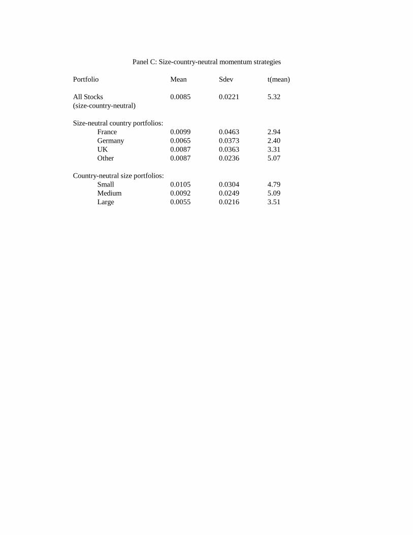
Panel C: Size-country-neutral momentum strategies


All Stocks 0.0085 0.0221 5.32(size-country-neutral)

Size-neutral country portfolios:France 0.0099 0.0463 2.94Germany 0.0065 0.0373 2.40UK 0.0087 0.0363 3.31Other 0.0087 0.0236 5.07

Country-neutral size portfolios:Small 0.0105 0.0304 4.79Medium 0.0092 0.0249 5.09Large 0.0055 0.0216 3.51

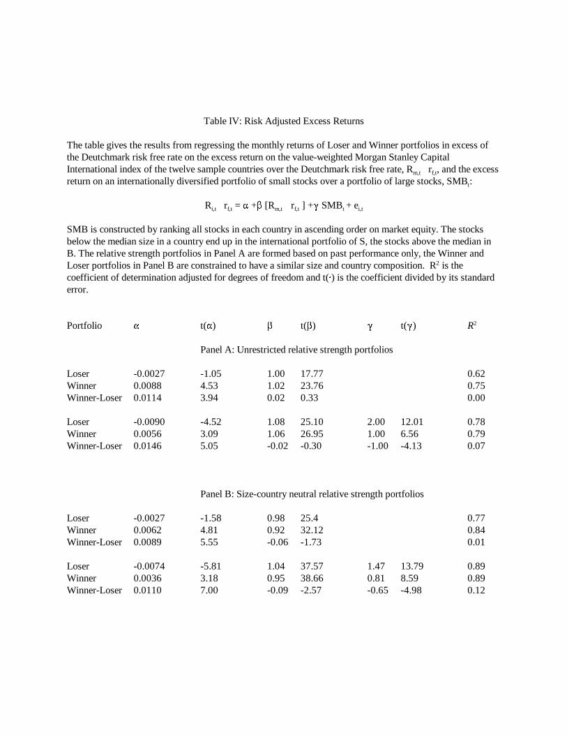
Table IV: Risk Adjusted Excess Returns

The table gives the results from regressing the monthly returns of Loser and Winner portfolios in excess ofthe Deutchmark risk free rate on the excess return on the value-weighted Morgan Stanley CapitalInternational index of the twelve sample countries over the Deutchmark risk free rate, R�r , and the excessm,t f,t

return on an internationally diversified portfolio of small stocks over a portfolio of large stocks, SMB :t

R �r = � +� [R �r ] +� SMB + ei,t f,t m,t f,t t i,t

SMB is constructed by ranking all stocks in each country in ascending order on market equity. The stocksbelow the median size in a country end up in the international portfolio of S, the stocks above the median inB. The relative strength portfolios in Panel A are formed based on past performance only, the Winner andLoser portfolios in Panel B are constrained to have a similar size and country composition. R is the2

coefficient of determination adjusted for degrees of freedom and t(#) is the coefficient divided by its standarderror.

Portfolio � t(�) � t(�) � t(�) R2

Panel A: Unrestricted relative strength portfolios

Loser -0.0027 -1.05 1.00 17.77 0.62Winner 0.0088 4.53 1.02 23.76 0.75Winner-Loser 0.0114 3.94 0.02 0.33 0.00

Loser -0.0090 -4.52 1.08 25.10 2.00 12.01 0.78Winner 0.0056 3.09 1.06 26.95 1.00 6.56 0.79Winner-Loser 0.0146 5.05 -0.02 -0.30 -1.00 -4.13 0.07

Panel B: Size-country neutral relative strength portfolios

Loser -0.0027 -1.58 0.98 25.4 0.77Winner 0.0062 4.81 0.92 32.12 0.84Winner-Loser 0.0089 5.55 -0.06 -1.73 0.01

Loser -0.0074 -5.81 1.04 37.57 1.47 13.79 0.89Winner 0.0036 3.18 0.95 38.66 0.81 8.59 0.89Winner-Loser 0.0110 7.00 -0.09 -2.57 -0.65 -4.98 0.12

Table V: Market Dependent Risk Adjusted Returns

The table gives the results from regressing the monthly returns of Loser and Winner portfolios in excess ofthe Deutchmark risk free rate on the excess return on the value-weighted Morgan Stanley CapitalInternational (MSCI) index of the twelve sample countries, R :m,t

R �r = � +� D [R �r ] +� (1�D ) [R �r ] + ei,t f,t t m,t f,t t m,t f,t i,t+ �

D is a dummy variable that is one if the MSCI return is positive in month t and zero otherwise. The relativet

strength portfolios in Panel A are formed based on past performance only, the Winner and Loser portfolios inPanel B are constrained to have a similar size and country composition. R is the coefficient of determination2

adjusted for degrees of freedom, and t(#) is the coefficient divided by its standard error.

Panel A: Unrestricted relative strength portfolios

Portfolio � t(�) � t(� ) � t(� ) R+ + � � 2

Loser -0.0065 -1.69 1.13 10.24 0.90 9.58 0.62Winner 0.0134 4.57 0.87 10.46 1.14 16.00 0.75Winner-Loser 0.0199 4.56 -0.25 -2.04 0.24 2.26 0.02

Panel B: Size/country neutral relative strength portfolios

Loser -0.0044 -1.65 1.03 13.68 0.94 14.51 0.77Winner 0.0098 5.05 0.80 14.52 1.01 21.43 0.85Winner-Loser 0.0141 5.88 -0.23 -3.37 0.07 1.26 0.05

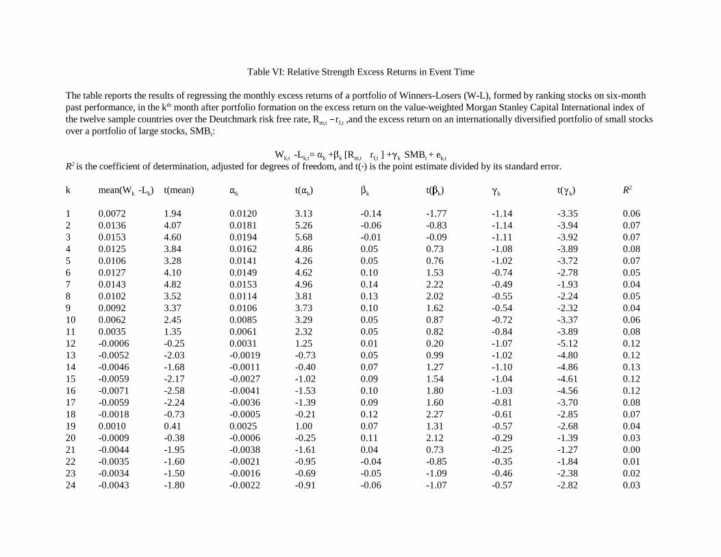
Table VI: Relative Strength Excess Returns in Event Time

The table reports the results of regressing the monthly excess returns of a portfolio of Winners-Losers (W-L), formed by ranking stocks on six-monthpast performance, in the k month after portfolio formation on the excess return on the value-weighted Morgan Stanley Capital International index ofth

the twelve sample countries over the Deutchmark risk free rate, R �r ,and the excess return on an internationally diversified portfolio of small stocksm,t f,t

over a portfolio of large stocks, SMB :t

W -L = � +� [R �r ] +� SMB + ek,t k,t k k m,t f,t k t k,t

R is the coefficient of determination, adjusted for degrees of freedom, and t(#) is the point estimate divided by its standard error. 2

k mean(W -L ) t(mean) � t(� ) � t(� ) � t(� ) Rk k k k k k k k2

1 0.0072 1.94 0.0120 3.13 -0.14 -1.77 -1.14 -3.35 0.062 0.0136 4.07 0.0181 5.26 -0.06 -0.83 -1.14 -3.94 0.073 0.0153 4.60 0.0194 5.68 -0.01 -0.09 -1.11 -3.92 0.074 0.0125 3.84 0.0162 4.86 0.05 0.73 -1.08 -3.89 0.085 0.0106 3.28 0.0141 4.26 0.05 0.76 -1.02 -3.72 0.076 0.0127 4.10 0.0149 4.62 0.10 1.53 -0.74 -2.78 0.057 0.0143 4.82 0.0153 4.96 0.14 2.22 -0.49 -1.93 0.048 0.0102 3.52 0.0114 3.81 0.13 2.02 -0.55 -2.24 0.059 0.0092 3.37 0.0106 3.73 0.10 1.62 -0.54 -2.32 0.0410 0.0062 2.45 0.0085 3.29 0.05 0.87 -0.72 -3.37 0.0611 0.0035 1.35 0.0061 2.32 0.05 0.82 -0.84 -3.89 0.0812 -0.0006 -0.25 0.0031 1.25 0.01 0.20 -1.07 -5.12 0.1213 -0.0052 -2.03 -0.0019 -0.73 0.05 0.99 -1.02 -4.80 0.1214 -0.0046 -1.68 -0.0011 -0.40 0.07 1.27 -1.10 -4.86 0.1315 -0.0059 -2.17 -0.0027 -1.02 0.09 1.54 -1.04 -4.61 0.1216 -0.0071 -2.58 -0.0041 -1.53 0.10 1.80 -1.03 -4.56 0.1217 -0.0059 -2.24 -0.0036 -1.39 0.09 1.60 -0.81 -3.70 0.0818 -0.0018 -0.73 -0.0005 -0.21 0.12 2.27 -0.61 -2.85 0.0719 0.0010 0.41 0.0025 1.00 0.07 1.31 -0.57 -2.68 0.0420 -0.0009 -0.38 -0.0006 -0.25 0.11 2.12 -0.29 -1.39 0.0321 -0.0044 -1.95 -0.0038 -1.61 0.04 0.73 -0.25 -1.27 0.0022 -0.0035 -1.60 -0.0021 -0.95 -0.04 -0.85 -0.35 -1.84 0.0123 -0.0034 -1.50 -0.0016 -0.69 -0.05 -1.09 -0.46 -2.38 0.0224 -0.0043 -1.80 -0.0022 -0.91 -0.06 -1.07 -0.57 -2.82 0.03

Figure I: Cumulative Payoff to Momentum Strategies in Event Time

The solid line gives the average cumulative payoff to a buy-and-hold strategy that invest aDeutchmark (DM) in a portfolio of Winners financed by a unit DM portfolio of Losers, in the k-thmonth after portfolio formation. The payoff is measured Pfennig (equals 0.01 DM). At the time offormation, the Winners and Losers are equally-weighted portfolios constructed to be both size-and country-neutral. They contain from each of the 36 size-country groups the top and bottomdecile of stocks ranked in ascending order based on past 6-month return. The dashed lines givethe 95% confidence interval of the average payoff, computed using autocorrelation consistentstandard errors.

I thank Ray Ball, Louis Chan, Jennifer Conrad, Eugene Fama, Narasimhan Jegadeesh, Ken*

French, N. Prabhala, Jake Thomas, Roberto Wessels, seminar participants at Erasmus Universiteit

Rotterdam, Katholieke Universiteit Leuven, the University of North Carolina, the University of

Pennsylvania, Rene Stulz, and an anonymous referee for their comments, and ARCAS-Wessels

Roll Ross for kindly providing the data.

See for example Chan (1988), Ball and Kothari (1989), Ball, Kothari and Shanken (1995),1

Conrad and Kaul (1993, 1996) , Chan, Hamao and Lakonishok (1991), Lakonishok, Schleifer and

Vishny (1994), DeLong Schleifer, Summers and Waldman (1990).

Foerster et al (1995) provide evidence on momentum strategies in the Canadian market.2

Although the sample is not comprehensive, and is biased to the larger firms in each market, there3

is no selection bias in the sense that the data are not backfilled.

An exception arises when a stock is delisted. In that case the liquidating proceeds are invested in4

the value weighted MSCI index of the 12 countries in the sample. The conclusions of the paper

are unchanged if the proceeds are re-invested in the remaining stocks in the same decile portfolio.

Return data are available from 1978, but two years are lost due to performance ranking: the5

J=12, K=12 strategy consists in part of positions taken 12 months ago based on prior 12-month

performance.

For example, Conrad and Kaul (1993) and Ball, Kothari and Wasley (1995) show that this bias6

overstates the profitability of contrarian strategies.

Allowing for a delayed market response due to non-synchronous trading does not change these7

conclusions.

This size differential is in part a manifestation of the continuation effect, because the J=6, K=68

relative strength portfolios at time t contain positions taken at time t-6. Of two firms that have

equal size but different past performance at time t-6, the firm with higher past returns will at time t

on average be larger than the firm with lower past returns because performance persists.

This is only approximately true. The relative strength portfolios consist of K separate holdings,9

and each of these K positions is only country-neutral at origination. Because the positions are not

rebalanced over time they lose their equal weighting in subsequent periods, due to performance

differences and as securities are added to (or removed from) the sample.

This is consistent with the relatively weak momentum in country index returns reported in10

Richards (1996), Bekaert et al (1996), and Ferson and Harvey (1996).

I also perform a similar analysis of sector momentum, by constructing sector-neutral portfolios11

based on assignments to 7 broad industry groups obtained from the Financial Times. The returns

on sector-neutral relative strength strategies were all positive, and significantly different from zero

for Basic Industries, Capital Goods, Consumer Goods and Finance. For the Energy,

Transportation and Utilities sectors, which contain relatively few stocks and hence poorly

diversified, the equality of Winner and Loser returns could not be rejected.

These size results are stronger than Jegadeesh and Titman (1993), and Asness (1995) find for12

the U.S., where relative strength portfolios of medium sized firms outperform both small and

large firms.

The SMB portfolio is constructed by sorting the sample firms by country on size in each month.13

Firms smaller than the median size in a country are assigned to the internationally diversified S

portfolio, the largest 50 percent to the B portfolio. SMB is the excess return of S minus B. The

average return and standard deviation of the international SMB portfolio are 0.29 and 1.16

percent per month between 1980 and 1995.

I am grateful to the referee for suggesting this point.14

I construct the (J=6, K=6) buy-and-hold U.S. momentum (W-L) portfolio using all available15

NYSE and AMEX firms on CRSP in the same way as the European W-L portfolio. The sample

average return and standard deviation of the U.S. momentum portfolio are 1.24 and 4.65 percent

per month between 1980 and 1995.

International Momentum Strategies K. Geert Rouwenhorst ...

Documents

Transcript of International Momentum Strategies K. Geert Rouwenhorst ...