EEccoonnoomm iiccss PPrrooggrraamm WWoorrkkiinngg PPaapp eerr SSeerr iieess

International Labor Cost Projections

Gad Levanon

Bert Colijn

Michael Paterra

Frank Steemers

Elizabeth Rust

The Conference Board

January 2016

EEPPWWPP ##1166 -- 0033

Economics Program

845 Third Avenue

New York, NY 10022-6679

Tel. 212-759-0900

www.conference-board .org/ economics

1

International Labor Cost Projections

Gad Levanon*, Bert Colijn, Michael Paterra,

Frank Steemers, and Elizabeth Rust

The Conference Board

845 Third Avenue, New York, NY 10022

Abstract

Differences in labor cost growth signal changes to an economy’s international

competitiveness as well as its workers’ comparative standard of living, yet there is

a scarcity of adequate models that project labor costs across countries. In this

paper we use a panel data set of 19 countries to forecast (1) labor cost growth, (2)

growth in wages and salaries (“pay for time worked”) and (3) average annual

wages from 2015 to 2020, using data from The Conference Board International

Labor Comparisons program. We compare the U.S. projections to other advanced

economies in Europe and Asia/Pacific.

Key Words: international, wage growth, labor compensation, manufacturing,

forecast, standard of living

*Corresponding author: Gad Levanon, Managing Director, Economic Outlook & Labor Markets,

The Conference Board, 845 Third Avenue, New York, NY 10022, gad.levanon@conference-

board.org. This research was supported by a grant from the Alfred P. Sloan Foundation. We are

also grateful to participants in the Workshop on International Labor and Productivity Comparisons

on October 15th 2015, Washington D.C, for their comments and suggestions.

2

1. Introduction

Wage growth is an important indicator of the strength of the economy and the well-being

of workers. It is closely tied to growth in individuals’ income and wealth, points to

changes in household consumption, and indicates the economy’s future cost

competitiveness relative to the rest of the world. All of these elements affect the

economy’s overall growth, making the forecasting of wage growth a useful economic

tool.

However, to our knowledge, such a wage forecasting has not yet been strongly developed

in the form of a predictive model. There exists a wealth of literature that links wage

growth to productivity growth, wage growth to inflation, wage growth to the strength of

labor institutions, and wage growth to unemployment, among other variables. Despite the

establishment of strong links between wage growth and these variables—both

theoretically and empirically—the literature still lacks a model with the ability to robustly

forecast wage growth. Some current models attempt to do this, but they variably focus

only on the short run or rely almost entirely on one or two variables.

In this paper we develop a model that takes into account the impact of inflation,

unemployment, labor productivity, the strength of employment protection, and output

growth in order to forecast wage growth annually from 2015 through 2020. To do so we

employ a panel dataset that covers 19 developed economies over a period of up to 20

years. We use three measures of labor compensation to estimate wage growth: (1) the

hourly labor cost in manufacturing series from The Conference Board International Labor

Comparisons (ILC) program, (2) pay for time worked (wages and salaries) in

manufacturing, also from the ILC program, and (3) average annual wages in the total

economy from the OECD.

The rest of this paper is organized as follows: First we review the existing literature on

the main correlates of wage growth which are the basis for the model’s theoretical

framework. Afterward, we discuss the data and methodology employed by our model.

This is followed by a discussion of the results.

3

2. Literature Review: Forecasting Growth in Labor Costs

2.1 Wage Growth and Productivity

The link between productivity growth and wage growth is well-established in the

literature. Standard microeconomic theory holds that an employer will hire workers up

until the point where the marginal product of labor is equal to the real wage. Workers’

wages are assumed to be equal to their marginal output. This carries two important

implications. First, if productivity increases while wages are held constant, employment

will increase as firms find it profitable to hire more workers and expand production.

Second, if the labor supply is fixed, an increase in demand for labor will lead to a rise in

wages.

An alternative theory is that of efficiency wages proposed by Shapiro and Stiglitz (1984),

which states that the causal relationship is the opposite, with wages affecting

productivity. This theory runs counter to traditional microeconomic theory, which implies

that productivity increases lead to wage increases. Shapiro and Stiglitz postulate that

above a certain wage, workers are discouraged from shirking their work and encouraged

to work more efficiently. Therefore, an ideal wage—one that is higher than the marginal

product of labor, but the lowest wage at which the worker is incentivized to work rather

than shirk—must exist. The level of the ideal wage is influenced by factors such as the

probability of being caught shirking and the level of unemployment compensation. It can

be difficult to disentangle which of the two theories predominates in practice: likely both

are in effect, but the influence of one or the other varies across countries.

Many authors have observed a growing gap between productivity growth and wage

growth over the past thirty years. Productivity growth has outpaced wage growth across

the member countries of the Organization for Economic Cooperation and Development

(OECD), though the extent once again varies by country, with the effect shown to be

particularly strong in the United States. Further discussion lies beyond the scope of this

paper.

Overall, the literature points to a positive relationship between productivity growth and

wage growth, although the strength of this link appears to have been declining recently

due to several factors. Thus, we include the growth rate of labor productivity in the

model, expecting positive labor productivity growth to increase the growth rate of labor

compensation.

2.2 Wage Growth and Inflation

There is a strong positive empirical link between wage growth and inflation. As with

productivity, the causal direction of this effect appears to go both ways. On the one hand,

there is strong evidence that inflation leads to wage growth, as rising prices and a higher

cost of living lead workers to demand higher wages from their employers so as not to

suffer decreased purchasing power. Many countries anticipate this effect by indexing

wages to the Consumer Price Index (CPI) so that wages will automatically rise with

prices. In such cases the link between wage growth and inflation is even more direct.

On the other hand, some evidence suggests that wage growth leads to inflation. As

workers bargain for higher wages, their wage growth begins to outpace their productivity

growth, stressing profits and imposing a greater cost on employers. As a result, firms

increase prices, thus passing on the impact to consumers, who in turn demand higher

4

wages—thus engendering the “wage-price spiral” described by Bronfenbrenner and

Holtzman (1965) and others.

Overall, the causal mechanism for the link between inflation and wage growth is less

important to the model than the simple fact that the two variables correlate positively, at

least in the short run. We include the annual growth rate of the consumer price index for

each country in the model as our measure of inflation, expecting inflation to be a strong

driver of wage growth.

2.3 Wage Growth and Labor Market Institutions

The strength of a country’s labor market institutions is also predictive. Union power and

coverage have a great influence on the level of wage bargaining and coordination

between workers, firms, and governments. There are two main causal mechanisms,

outlined by authors such as Nickell, Nunziata, Ochel, and Quintini (2001). One is that

strong unions encourage direct wage bargaining between labor and industry by

supporting workers’ demands for higher wages and arguing on behalf of workers. The

way in which this may affect wage growth is therefore rather evident: stronger unions

lead to greater wage growth. Our original inclusion of a union density variable in the

model is an attempt to quantify the power of unions and witness their effect on wage

growth across countries. However, union density ultimately proved to not be a significant

predictor of wage growth, and we excluded it from the final model.

The second way in which unions affect wage growth is through their influence on

employment protection legislation. In general, countries with stronger labor unions also

have strong employment protection legislation; unions have bargained with governments

over many years to secure these measures for the benefit of their members: employed

workers.

Strong employment protection legislation (EPL) is thus linked positively to wage growth

by several means. One is simply that a high degree of EPL is indicative of strong unions

since unions were the entity most likely to lobby for EPL in the first place. As the

presence of unions directly leads to greater wage bargaining, the two go hand in hand. A

second cause is that strong EPL lowers inflows into unemployment by reducing

involuntary separations. If unemployment is kept low, wages are likely to increase (a

phenomenon highlighted in the next section). However, strong EPL may also result in a

counteracting effect on unemployment: if firms are reluctant to hire workers for fear of

facing later obstacles to laying off workers in a downturn, EPL may reduce the efficiency

of job matching and keep unemployment artificially above the non-accelerating inflation

rate of unemployment (NAIRU). As a result, it is not clear which of the two contradictory

effects of strong EPL predominates.

Empirically, the link between strong employment protection legislation and wage growth

is positive, despite the two-way theoretical explanation for the relation. It is therefore

most likely that employment protection legislation has a direct impact on pay because it

raises the job security of current employees, which increases their leverage for

demanding higher wages.

2.4 Wage Growth and Unemployment

The link between wage growth and unemployment is both central to economic theory and

frequently debated, such that the consensus on the link between the two variables has

evolved over time. Prior to the 1970s, the theory of the Phillips Curve dominated in the

5

literature. This idea holds that there exists an inverse relationship between inflation and

unemployment. Since inflation and unemployment are in turn tied to other factors, the

Phillips Curve has implications far beyond these two variables. For example, since

inflation and wage growth are closely tied, the Phillips Curve also implies a relationship

between wage growth and unemployment—for the most part, an inverse one.

The Phillips Curve has always been limited in that it describes an observed empirical

relationship without positing a credible theoretical explanation. In the 1970s even its

empirical foundations began to break down, as most developed economies were beset by

simultaneously high inflation and unemployment. This prompted a search for other ways

of explaining changes in unemployment, at the same time as monetarist ideas came to the

forefront of the literature.

The non-accelerating inflation rate of unemployment (NAIRU) is one theory posed in

response to this need. The NAIRU refers to the level of unemployment below which

inflation will rise. It is related to an earlier hypothesis, the natural rate of unemployment,

posed by Friedman (1968), which states that any given labor market structure must

involve a certain level of unemployment caused by both frictional and structural factors.

If fiscal and monetary policy tries to target an unemployment rate below the economy’s

natural rate, it will only result in greater inflation.

With a strong basis for the inverse relation between wage growth and unemployment,

several authors have set out to determine the causal direction of this relationship. Altonji

and Ashenfelter (1980) conclude that it is difficult to attribute movements in

unemployment to aggregate deviations in future real wage rates. Later, however,

Blanchflower and Oswald (1989) find evidence for an empirical relationship between real

wage rates and unemployment in the United States and United Kingdom, which they

name the wage curve. Drawing from a number of microeconomic databases, they find

that the relationship is negative at lower levels of unemployment, but becomes horizontal

for higher unemployment levels. It follows that wage flexibility is present mainly at low

levels of unemployment. The authors posit the theoretical explanation that under high

levels of unemployment, workers lose the capacity for wage bargaining.

Taking Blanchflower and Oswald’s findings into account, other authors have explored

the relationship between wages and unemployment, with an eye toward the effects of

unemployment persistence and long-term unemployment. Gottfries and Horn (1987)

earlier describe a mechanism for how unemployment leads to persistent unemployment,

and how persistent unemployment actually contributes to greater wage growth. When a

contractionary shock occurs in the previous period, workers are laid off; with fewer

workers employed, wages can be raised in the current period without any substantial

increase in the likelihood that an employed worker loses his job. With higher wages,

fewer currently unemployed workers will be hired, and thus the original contractionary

shock results in a persistent negative effect on unemployment—at a higher wage rate.

The authors make reference to the notions that more permanently attached workers have

greater wage bargaining power, and that employed workers are rarely exchanged for

unemployed workers (due to seniority systems, turnover costs, and union power), but do

not explore these assumptions in great detail.

Krueger, Cramer, and Cho (2014) study these assumptions more directly and find that

they are supported empirically by recent data from the US labor market. They explore

data on the long-term unemployed in the United States and find that the unemployed are

6

progressively more likely to remain unemployed as their duration of unemployment

increases. The authors attribute this effect to various causes, including loss of bargaining

power, discrimination against the unemployed by hiring managers, as well as

discouragement and loss of self-confidence. The broader implications of these findings,

as suggested by the authors, are that the wage Phillips curve breaks down as the share of

permanently unattached workers rises. The wage curve relationship is still valid,

however, when it comes to short-term unemployment.

The literature thus reveals that, on the whole, the wage curve describes an inverse

relationship between wage growth and unemployment. However, this relationship may

break down when there exists a higher share of the labor force that is permanently

unattached.

2.5 Wage Growth and Growth in the Labor Force

Similar theoretical underpinnings exist between wage growth and unemployment as

between wage growth and labor force growth. Just as high unemployment—an excess of

labor—leads to reduced wage bargaining power for workers, so does labor force growth

contribute to a dampening of wage growth as workers lose their leverage, in light of

firms’ greater choice of employees. Growth in the labor force is affected by a number of

factors, including new groups (such as women and immigrants) entering the labor force,

as well as broader demographic factors such as population ageing, which leads to a

decline in size of the labor force. The relationship between wage growth and labor force

growth is therefore expected to be negative. Due to lack of explanatory power, though,

we ultimately excluded labor force growth from the model.

2.6 Other Wage Forecasting Models

Apart from theoretical models analyzing the main drivers of wage growth, we have found

two other existing models intended to forecast wage growth across countries. One model

forms part of the OECD’s Economic Outlook, and projects wage growth for all OECD

economies. It employs a proprietary model called the NiGEM—designed to incorporate a

large number of variables at once—combined with several short-term indicator models,

to forecast wage growth for the upcoming three years. The large number of variables can

be classified into four main areas: domestic expenditures; employment, wages, and

prices; output gaps; and foreign trade and balance of payments. While the model includes

a great variety and number of variables, such complexity limits its long-term forecasting

power. Forecasts must be continually reassessed to adjust for changes to each of the

many indicators employed. As a result, reasonable forecasts can only be made for three

years at a time.

PricewaterhouseCoopers (PWC) models a forecast of wage growth across 21 countries,

including both developed and emerging economies. Unlike the OECD’s model, it limits

its prediction to one major variable but projects forward until 2030. It relies on a basic

assumption of a strong correlation between labor productivity growth and wage growth

and therefore incorporates productivity growth as its exclusive main variable. Given the

wage-productivity gap that has emerged in developed economies, a downward

adjustment in wage forecasts is made for those countries. The adjustment is not made for

the developing economies included in the model. PWC also incorporates the effects of

long-term trends in the real exchange rate for each country as a secondary variable, while

acknowledging that exchange rate forecasts are subject to a great deal of uncertainty. The

main shortcoming of this model is its reliance on one major variable. While it projects far

into the future, this long-term anticipation may come at the expense of close precision

7

and accuracy. PWC themselves admit that their model is a better predictor of broad

trends than precise point forecasts.

8

3. Conceptual Framework

Wages comprise only part of overall labor costs, which we define as the total costs

incurred by a firm to employ labor. Labor costs include not only direct pay but also social

insurance expenditures and labor-related taxes. Direct pay encompasses all payments

made directly to the worker before payroll deductions, and consists of both pay for time

worked (wages) and directly-paid benefits. Social insurance expenditures refer to the

value of social contributions incurred by employers in order to secure entitlement to

social benefits for their employees. Labor-related taxes refer to taxes on payrolls or

employment, including those that do not directly benefit workers. Our data, taken from

the International Labor Comparisons program of The Conference Board, include nearly

all labor costs incurred by employers; however, it does not include indirect costs such as

recruitment, vocational training, and maintenance of company-provided facilities.

However, these costs typically amount to less than two percent of total labor costs.

Using series from the ILC program, we forecast the growth rate in both labor cost and

wages (“pay for time worked”) in the manufacturing sector. We focused on the

manufacturing sector for two reasons: (1) the internationally comparable data provided

by the ILC program lends itself to build a model with internationally comparable

forecasts, and (2) labor compensation growth in the manufacturing sector is a key

component to a country’s international competitiveness. Moreover, the Balassa-

Samuelson effect would argue that wage increases in non-tradable industries are

impacted by tradable industries.

To provide an alternative for comparison, we also used the total economy annual average

wages series from the OECD as an additional dependent variable.

Since our estimation is based on annual data we estimate nominal wages as opposed to

real wages. In an annual frequency, real wages are dominated by movement in volatile

components of inflation, such as energy, which have very little to do with the decisions of

employers regarding the compensation schedule in their organizations.

3.1 Data In our analysis we use a balanced panel dataset of 19 advanced economies

1 containing

data from 1985 to 2013 for labors costs and total average wages and data up to 2014 for

“pay for time worked’ wages. Our dependent variables include:

Nominal annual growth rate of labor cost per hour in manufacturing2 from the

ILC program,

Nominal annual growth rate of wages and salaries (“pay for time worked” in

manufacturing from the ILC program, and

1 Included economies (Earliest year of data available): Australia (1991); Austria (1997); Belgium

(1970); Canada (1970); Denmark (1972); Finland (1974); France (1970); Germany (1991); Greece

(1997); Ireland (1997); Italy (1970); Japan (1971); Netherlands (1970); New Zealand (1997);

Portugal (1997); Spain (1980); Switzerland (1997); the United Kingdom (1970); and the United

States (1980). 2 ILC time series for hourly cost, national currency national currency basis (Table 7, International

Comparisons of Manufacturing Productivity & Unit Labor Cost Trends, 2012) used to trend back

ILC hourly labor compensation in manufacturing, national currency basis, for 1970-1995 (or as

early as possible).

9

Nominal annual growth rate in the average annual wages for the total economy

from the OECD.

All level data is represented in national currency. For countries using the euro, the fixed

euro-national currency exchange rate was used to trend back pre-euro years so that all

data is in euros. Level data was transformed using natural logarithms to calculate a year

to year growth rate. The ILC program adjusts all data to adhere to U.S. data standards in

order to make data directly comparable across countries.

As outlined in the literature review, we use several explanatory variables to construct our

model of labor compensation growth:

Labor Productivity

Across all countries, the evidence reveals that productivity and wages are positively

linked, regardless of the causal mechanism responsible for the correlation. For this reason

productivity is considered as a key variable for our model. Since there is usually a delay

between increases in worker productivity and the resulting negotiations for higher wages,

we tested both a one-year lag of labor productivity in our model, but the current years

labor productivity ultimately had more explanatory power in the model. We use labor

productivity data for the total economy from The Conference Board Total Economy

Database™ (TED). While labor productivity data for the manufacturing sector would

have been ideal, we chose to employ the TED data because projections of labor

productivity through 2025 were readily available3.

Inflation

We calculated the annual growth rate of the national consumer price index4 for each

economy to estimate the annual inflation rate. We used data from the ILC program5

where available. In accordance with economic theory, we expect the coefficient of

inflation to be positive; as the literature suggests, there is a strong positive empirical link

between wage growth and inflation. When prices increase across the economy, workers

demand increases in nominal wages in order to maintain—if not increase—their

purchasing power.

Gross Domestic Product (GDP)

We calculate the logarithmic growth rate of GDP using gross domestic product data for

the total economy from The Conference Board Total Economy Database™. In line with

economic theory, we expect the coefficient to be positive; as the economy grows (as a

result of labor productivity gains or other short-term forces), workers negotiate to capture

some of the gains through increases in their compensation. Thus, we include a one-year-

lag of GDP growth in the model, as there is some lag between revenue gains and

increases in compensation.

Unemployment Gap

The literature has established an inverse relationship between wage growth and

unemployment. As unemployment declines, wage growth tends to accelerate. Especially

considering that elevated unemployment levels have declined at varying rates in the years

since the Great Recession, including a measure of unemployment in our model is

3 Projecting labor productivity trends was outside the scope of this paper.

4 The national retail price index (RPI) is used for the United Kingdom.

5 https://www.conference-board.org/ilcprogram/consumerpricesannual

10

necessary to explain the variation in labor compensation growth among advanced

economies.

In the model we do not include unemployment directly but rather the gap between the

unemployment rate and the natural rate of unemployment for each economy. This gap

measure enables us to better capture the amount of “slack” in each respective labor

market in a given year. To calculate the unemployment gap, we subtract the natural rate

of unemployment from the annual unemployment rate using data from the OECD. Since

the natural rate of unemployment is specific to each country, we use the NAIRU (non-

accelerating inflation rate of unemployment) from the OECD as a proxy for the natural

rate of unemployment.

There are two reasons for using the unemployment gap in the model instead of simply

including the unemployment rate. First, the unemployment gap measures the level of

slack in an economy better than the unemployment rate alone. Due to variations in

structural unemployment, unemployment rates are not always directly comparable

between countries: 15 percent unemployment in Spain reflects a very different situation

than 15 percent unemployment in the United States, for example. By using the gap

between the current unemployment rate and the natural rate of unemployment, we can

capture the relative differences in the labor market situation between countries in a

meaningful way, which enables more robust measurement of the impact of

unemployment on wage growth.

Secondly, the natural rate of unemployment varies over time in each country. Changes in

the number of long-term unemployed, unemployment benefits and employment

regulations, among other factors, all of which fluctuate over time, can affect the natural

rate of unemployment, and thus the meaning of a given unemployment rate. By using the

unemployment gap instead of the unemployment rate, we are able to capture those

variations over time and to project them into the future.

We expect the coefficient of the unemployment gap to be negative. An expanding

unemployment gap reflects a labor market with increasing slack and, correspondingly,

reflects workers’ diminishing bargaining power, resulting in less pressure on firms to

increase wages.

3.2 Model Selection We went through several iterations to develop a model with the greatest explanatory

power given our available data and that also aligned closely with the economic theory

laid out in the literature. The model we used to forecast hourly labor cost growth is as

follows:

𝐿𝑎𝑏𝑜𝑟 𝐶𝑜𝑠𝑡 𝑔𝑟𝑜𝑤𝑡ℎ𝑖𝑡̂

= 𝛽0 + 𝛽1 ∗ 𝐼𝑛𝑓𝑙𝑎𝑡𝑖𝑜𝑛𝑖𝑡 + 𝛽2 ∗ 𝑈𝑛𝑒𝑚𝑝𝑙𝑜𝑦𝑚𝑒𝑛𝑡 𝐺𝑎𝑝𝑖𝑡 + 𝛽3

∗ 𝐺𝐷𝑃 𝑔𝑟𝑜𝑤𝑡ℎ𝑖𝑡 + 𝐵4 ∗ 𝐿𝑎𝑏𝑜𝑟 𝐶𝑜𝑠𝑡 𝑔𝑟𝑜𝑤𝑡ℎ𝑖,𝑡−1 + 𝛽5

∗ 𝐿𝑎𝑏𝑜𝑟 𝑃𝑟𝑜𝑑𝑢𝑐𝑡𝑖𝑣𝑖𝑡𝑦 𝑔𝑟𝑜𝑤𝑡ℎ𝑖𝑡

The model we used to forecast hourly pay for time worked growth is as follows:

11

𝑃𝑎𝑦 𝐹𝑜𝑟 𝑇𝑖𝑚𝑒 𝑊𝑜𝑟𝑘𝑒𝑑 𝑔𝑟𝑜𝑤𝑡ℎ𝑖𝑡̂

= 𝛽0 + 𝛽1 ∗ 𝐼𝑛𝑓𝑙𝑎𝑡𝑖𝑜𝑛𝑖𝑡 + 𝛽2 ∗ 𝑈𝑛𝑒𝑚𝑝𝑙𝑜𝑦𝑚𝑒𝑛𝑡 𝐺𝑎𝑝𝑖𝑡 + 𝛽3

∗ 𝐺𝐷𝑃 𝑔𝑟𝑜𝑤𝑡ℎ𝑖𝑡 + 𝐵4 ∗ 𝑃𝑎𝑦 𝐹𝑜𝑟 𝑇𝑖𝑚𝑒 𝑊𝑜𝑟𝑘𝑒𝑑 𝑔𝑟𝑜𝑤𝑡ℎ𝑖,𝑡−1 + 𝛽5

∗ 𝐿𝑎𝑏𝑜𝑟 𝑃𝑟𝑜𝑑𝑢𝑐𝑡𝑖𝑣𝑖𝑡𝑦 𝑔𝑟𝑜𝑤𝑡ℎ𝑖,𝑡

Finally, the model we used to forecast average annual wage growth is as follows:

𝐴𝑛𝑛𝑢𝑎𝑙 𝐴𝑣𝑒𝑟𝑎𝑔𝑒 𝑊𝑎𝑔𝑒𝑠 𝑔𝑟𝑜𝑤𝑡ℎ𝑖𝑡̂

= 𝛽0 + 𝛽1 ∗ 𝐼𝑛𝑓𝑙𝑎𝑡𝑖𝑜𝑛𝑖𝑡 + 𝛽2 ∗ 𝑈𝑛𝑒𝑚𝑝𝑙𝑜𝑦𝑚𝑒𝑛𝑡 𝐺𝑎𝑝𝑖𝑡 + 𝛽3

∗ 𝐺𝐷𝑃 𝑔𝑟𝑜𝑤𝑡ℎ𝑡 + 𝐵4 ∗ 𝐴𝑛𝑛𝑢𝑎𝑙 𝐴𝑣𝑒𝑟𝑎𝑔𝑒 𝑊𝑎𝑔𝑒 𝑔𝑟𝑜𝑤𝑡ℎ𝑖,𝑡−1 + 𝛽5

∗ 𝐿𝑎𝑏𝑜𝑟 𝑃𝑟𝑜𝑑𝑢𝑐𝑡𝑖𝑣𝑖𝑡𝑦 𝑔𝑟𝑜𝑤𝑡ℎ𝑖𝑡

We include the lag dependent in each model since we expect that the previous year of

labor cost can have a strong influence on the current value. Previous iterations included

other potential explanatory variables such as tertiary education, union density,

employment protection legislation, and urbanization, which were statistically

insignificant and/or reduced the explanatory power of the model. It is possible that

institutional factors would have found to have more of an impact on the level of wages as

opposed to the growth rate of wages. There is relatively small changes overtime in the

institutional variables, which makes it difficult to disentangle noise from signal in

estimations over time.

We expected union density to have a positive impact on wage growth, based on the

assumption that the more unionized workers in an economy, the stronger the bargaining

power of workers to negotiate higher wages. We tried both the current union density and

a one-year lag of union density in the model, and while the coefficient was positive in

both cases, neither coefficient was statistically significant at any acceptable level of

significance. Thus, we excluded a measure of union density. In addition, we tried to

include a measure for employment protection legislation (i.e., strength of individual

dismissals protection) reasoning that unions have bargained with governments over many

years to secure benefits and secure contracts for employed workers. However,

employment protection legislation, measured by each country’s deviation from the mean,

was insignificant.

3.3 Estimation Beyond the choice of explanatory variables forecasting requires estimating a set of

coefficients, based on historical data and attaching them to forecasts of the explanatory

variables. The forecast could vary depending on the method of estimation being used, the

sample of countries used in the estimation, and the time sample used in the estimation.

First of all, we choose to use panel data estimations to exploit all available information

among countries and years. We use Hausman’s (1978) specification test and find that the

fixed effects model is more appropriate than the random effects model. Next, we check if

the fixed effects among countries differ using an F-test of joint significance. The test

shows that the fixed effects model is the right model to use. We also use the entire sample

of countries. In further work we will explore how the results change if we allow for

estimation of groups of countries. Lastly, we include the lag dependent in the model since

we expect that the previous year of labor cost can have a strong influence on the current

value. We decide not to use a dynamic panel data model to correct for a bias that arises

12

by using the lag dependent in a panel data models.6 Following the suggestions of Judson

and Owen (1999), we reason that the long time span of our data reduces the bias to a

minimum. In addition, after running dynamic panel data models we ended up with

different estimation problems.7

It turns out that the coefficients we choose for forecasting labor cost heavily depend on

the length of the sample. As we change the starting year of the sample, the coefficients

vary significantly. A lot of it is a result of the change in the inflation environment during

the 1980’s and 1990’s.

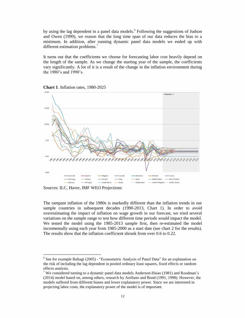
Chart 1. Inflation rates, 1980-2025

Sources: ILC, Haver, IMF WEO Projections

The rampant inflation of the 1980s is markedly different than the inflation trends in our

sample countries in subsequent decades (1990-2013, Chart 1). In order to avoid

overestimating the impact of inflation on wage growth in our forecast, we tried several

variations on the sample range to test how different time periods would impact the model.

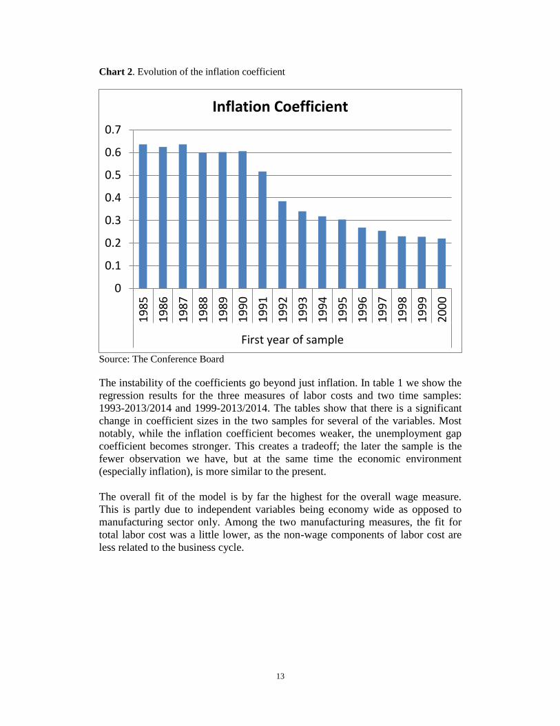
We tested the model using the 1985-2013 sample first, then re-estimated the model

incrementally using each year from 1985-2000 as a start date (see chart 2 for the results).

The results show that the inflation coefficient shrunk from over 0.6 to 0.22.

6 See for example Baltagi (2005) - “Econometric Analysis of Panel Data” for an explanation on

the risk of including the lag dependent in pooled ordinary least squares, fixed effects or random

effects analysis. 7 We considered turning to a dynamic panel data models Anderson-Hsiao (1981) and Roodman’s

(2014) model based on, among others, research by Arellano and Bond (1991, 1998). However, the

models suffered from different biases and lower explanatory power. Since we are interested in

projecting labor costs, the explanatory power of the model is of important.

13

Chart 2. Evolution of the inflation coefficient

Source: The Conference Board

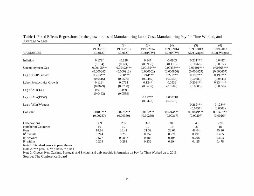
The instability of the coefficients go beyond just inflation. In table 1 we show the

regression results for the three measures of labor costs and two time samples:

1993-2013/2014 and 1999-2013/2014. The tables show that there is a significant

change in coefficient sizes in the two samples for several of the variables. Most

notably, while the inflation coefficient becomes weaker, the unemployment gap

coefficient becomes stronger. This creates a tradeoff; the later the sample is the

fewer observation we have, but at the same time the economic environment

(especially inflation), is more similar to the present.

The overall fit of the model is by far the highest for the overall wage measure.

This is partly due to independent variables being economy wide as opposed to

manufacturing sector only. Among the two manufacturing measures, the fit for

total labor cost was a little lower, as the non-wage components of labor cost are

less related to the business cycle.

0

0.1

0.2

0.3

0.4

0.5

0.6

0.71

98

5

19

86

19

87

19

88

19

89

19

90

19

91

19

92

19

93

19

94

19

95

19

96

19

97

19

98

19

99

20

00

First year of sample

Inflation Coefficient

14

Table 1. Fixed Effects Regressions for the growth rates of Manufacturing Labor Cost, Manufacturing Pay for Time Worked, and

Average Wages (1) (2) (3) (4) (5) (6)

1993-2013 1999-2013 1993-2014 1999-2014 1993-2013 1999-2013

VARIABLES ∆Ln(LC) ∆Ln(LC) ∆Ln(PTW) ∆Ln(PTW) ∆Ln(Wages) ∆ Ln(Wages)

Inflation 0.172* -0.128 0.147 -0.0903 0.211*** 0.0487

(0.104) (0.124) (0.0955) (0.113) (0.0766) (0.0912)

Unemployment Gap -0.00195*** -0.00422*** -0.00185*** -0.00433*** -0.00191*** -0.00368***

(0.000645) (0.000913) (0.000602) (0.000856) (0.000459) (0.000667)

Lag of GDP Growth 0.253*** 0.268*** 0.244*** 0.225*** 0.198*** 0.199***

(0.0516) (0.0596) (0.0489) (0.0558) (0.0389) (0.0443)

Labor Productivity Growth 0.118* 0.0764 0.124* 0.0536 0.209*** 0.234***

(0.0679) (0.0758) (0.0637) (0.0709) (0.0500) (0.0559)

Lag of ∆Ln(LC) 0.0701 -0.0593

(0.0492) (0.0589)

Lag of ∆Ln(PTW) 0.122** 0.000218

(0.0478) (0.0578)

Lag of ∆Ln(Wages) 0.262*** 0.123**

(0.0457) (0.0603)

Constant 0.0180*** 0.0275*** 0.0162*** 0.0244*** 0.00849*** 0.0146***

(0.00287) (0.00350) (0.00259) (0.00317) (0.00207) (0.00264)

Observations 369 285 378 300 348 270

Number of Countries 19 19 19 19 18 18

F-test 18.16 20.41 21.39 23.01 48.04 45.26

R2 overall 0.244 0.253 0.257 0.271 0.491 0.485

R2 between 0.577 0.0897 0.488 0.104 0.798 0.603

R2

within 0.208 0.281 0.232 0.294 0.425 0.478

Note 1: Standard errors in parentheses

Note 2: *** p<0.01, ** p<0.05, * p<0.1

Note 3: Greece, New Zealand, Portugal, and Switzerland only provide information on Pay for Time Worked up to 2013.

Source: The Conference Board

15

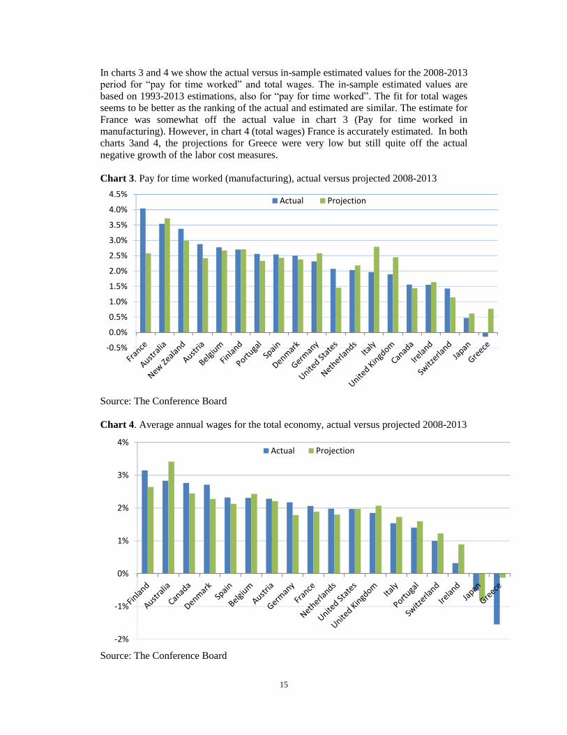
In charts 3 and 4 we show the actual versus in-sample estimated values for the 2008-2013

period for “pay for time worked” and total wages. The in-sample estimated values are

based on 1993-2013 estimations, also for “pay for time worked”. The fit for total wages

seems to be better as the ranking of the actual and estimated are similar. The estimate for

France was somewhat off the actual value in chart 3 (Pay for time worked in

manufacturing). However, in chart 4 (total wages) France is accurately estimated. In both

charts 3and 4, the projections for Greece were very low but still quite off the actual

negative growth of the labor cost measures.

Chart 3. Pay for time worked (manufacturing), actual versus projected 2008-2013

Source: The Conference Board

Chart 4. Average annual wages for the total economy, actual versus projected 2008-2013

Source: The Conference Board

-0.5%

0.0%

0.5%

1.0%

1.5%

2.0%

2.5%

3.0%

3.5%

4.0%

4.5%Actual Projection

-2%

-1%

0%

1%

2%

3%

4%Actual Projection

16

3.4 Forecast To forecast wage growth through 2020 we use projections of our independent variables

from several different sources. Inflation projections for 2015-2019 are from the

International Monetary Fund (IMF) World Economic Outlook 2015. We extend the

inflation rate projected for 2019 through 2020, based on the assumption that each

country’s central bank will achieve its long-term inflation target by 2020.

We use projections of GDP and labor productivity from The Conference Board Total

Economy Database™ for 2015-2019. Projections of the unemployment gap (i.e., the gap

between the unemployment rate and the natural rate of unemployment) are based on IMF

projections of the unemployment rate and the NAIRU. The Conference Board adjusted

the IMF projections in order to reflect our expectations of declining unemployment and

the shifting natural rates of unemployment for the countries in our sample.

17

4. Results

Considering inflation stabilized in all of our sample countries during the 1990s, in the

following we proceed with the 1993-2013 sample period for the model in order to make

projections for 2015-2020.

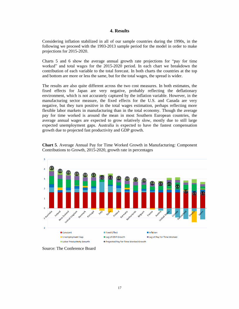
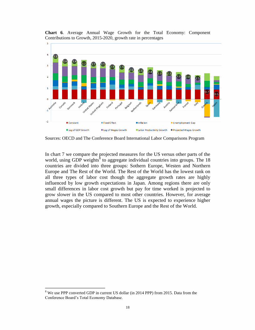
Charts 5 and 6 show the average annual growth rate projections for “pay for time

worked” and total wages for the 2015-2020 period. In each chart we breakdown the

contribution of each variable to the total forecast. In both charts the countries at the top

and bottom are more or less the same, but for the total wages, the spread is wider.

The results are also quite different across the two cost measures. In both estimates, the

fixed effects for Japan are very negative, probably reflecting the deflationary

environment, which is not accurately captured by the inflation variable. However, in the

manufacturing sector measure, the fixed effects for the U.S. and Canada are very

negative, but they turn positive in the total wages estimation, perhaps reflecting more

flexible labor markets in manufacturing than in the total economy. Though the average

pay for time worked is around the mean in most Southern European countries, the

average annual wages are expected to grow relatively slow, mostly due to still large

expected unemployment gaps. Australia is expected to have the fastest compensation

growth due to projected fast productivity and GDP growth.

Chart 5. Average Annual Pay for Time Worked Growth in Manufacturing: Component

Contributions to Growth, 2015-2020, growth rate in percentages

Source: The Conference Board

18

Chart 6. Average Annual Wage Growth for the Total Economy: Component

Contributions to Growth, 2015-2020, growth rate in percentages

Sources: OECD and The Conference Board International Labor Comparisons Program

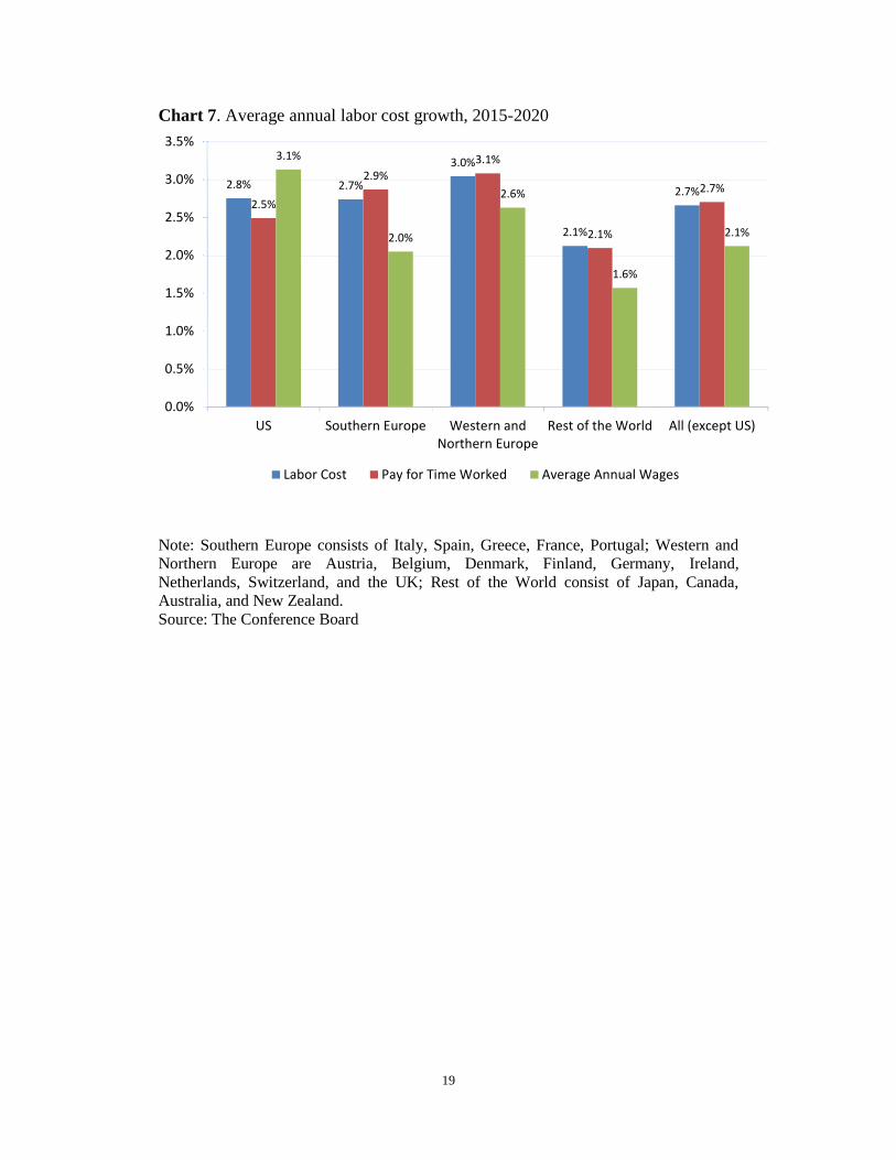
In chart 7 we compare the projected measures for the US versus other parts of the

world, using GDP weights8 to aggregate individual countries into groups. The 18

countries are divided into three groups: Sothern Europe, Westen and Northern

Europe and The Rest of the World. The Rest of the World has the lowest rank on

all three types of labor cost though the aggregate growth rates are highly

influenced by low growth expectations in Japan. Among regions there are only

small differences in labor cost growth but pay for time worked is projected to

grow slower in the US compared to most other countries. However, for average

annual wages the picture is different. The US is expected to experience higher

growth, especially compared to Southern Europe and the Rest of the World.

8 We use PPP converted GDP in current US dollar (in 2014 PPP) from 2015. Data from the

Conference Board’s Total Economy Database.

19

Chart 7. Average annual labor cost growth, 2015-2020

Note: Southern Europe consists of Italy, Spain, Greece, France, Portugal; Western and

Northern Europe are Austria, Belgium, Denmark, Finland, Germany, Ireland,

Netherlands, Switzerland, and the UK; Rest of the World consist of Japan, Canada,

Australia, and New Zealand.

Source: The Conference Board

2.8% 2.7%

3.0%

2.1%

2.7% 2.5%

2.9%

3.1%

2.1%

2.7%

3.1%

2.0%

2.6%

1.6%

2.1%

0.0%

0.5%

1.0%

1.5%

2.0%

2.5%

3.0%

3.5%

US Southern Europe Western andNorthern Europe

Rest of the World All (except US)

Labor Cost Pay for Time Worked Average Annual Wages

20

5. Conclusion

In this paper we attempt a first step at building an econometric model to forecast

compensation growth using a panel data method. We highlight several challenges, in

particular coefficient instability over time. We use both measures of wages in the total

economy and manufacturing compensation measures utilizing The Conference Board’s

ILC dataset.

We find that the overall fit of the model is by far the highest for the overall wage measure

compared with manufacturing measures. We also find that outside Japan, the Southern

European countries are projected to have the slowest compensation growth, mostly due to

still large expected unemployment gaps. Compensation in the US is projected to be a

little faster than average.

Further possible extensions of this work should focus on comparing in-sample and out-

of-sample forecast. In addition, different methods and samples should be explored. In

particular, how will projections change when moving from a country panel data model to

groups or perhaps individual country forecasts?

Finally, in this paper we focused on forecasting labor cost growth. In future extensions it

would be interesting to estimate the level of labor compensation and the impact of

institutional factors on such measures.

21

References

Altonji, Joseph, and Orley Ashenfelter. "Wage Movements and the Labour Market

Equilibrium Hypothesis." Economica 47, no. 187 (1980): 217-45.

Blanchflower, David G., and Andrew J. Oswald. "The Wage Curve."Centre for Labour

Economics, London School of Economics and Political Science, 1989, 1-49.

Blanchflower, David G., and Andrew J. Oswald. "An Introduction to the Wage

Curve."Journal of Economic Perspectives 9, no. 3 (1995): 153-167.

Blanchflower, David G., and Andrew J. Oswald. "The Wage Curve Reloaded." National

Bureau of Economic Research, Working Paper 11338 (2005).

Bronfenbrenner, Martin, and F. D. Holzman. "A Survey of Inflation Theory." Surveys of

Economic Theory 1 (1965): 46-107.

Darrat, Ali F. "Wage Growth and the Inflationary Process: A Reexamination." Southern

Economic Journal 61, no. 1 (1994): 181-90.

Friedman, Milton. "The Role of Monetary Policy." The American Economic Review 58,

no. 1 (1968): 1-17.

Fuess, Scott M., and Meghan Millea. "Pay and Productivity in “Corporatist” Germany."

Journal of Labor Research 27, no. 3 (2006): 397-409.

Gottfries, Nils, and Henrik Horn. "Wage Formation and the Persistence of

Unemployment." Economic Journal 97, no. 388 (1987): 877-84.

Judson, Ruth A., and Owen, Ann L. (1999). “Estimating Dynamic Panel Data Models: A

Guide for Macroeconomists.” Economics Letters 65: 9-15.

Kaldor, Nicholas. "A Model of Economic Growth." The Economic Journal 67, no. 268

(1957): 591-624.

Karabarbounis, Loukas, and Brent Neiman. "The Global Decline of the Labor Share."

The Quarterly Journal of Economics 129, no. 1 (2013): 61-103.

Krueger, Alan B., Judd Cramer, and David Cho. "Are the Long-Term Unemployed on the

Margins of the Labor Market?" Brookings Papers on Economic Activity, 2014.

Lopez-Villavicencio, Antonia, and Jose Ignacio Silva. "Employment Protection and the

Non-Linear Relationship Between the Wage-Productivity Gap and

Unemployment." Scottish Journal of Political Economy 58, no. 2 (2011): 200-20.

Mehra, Yash P. "Wage Growth and the Inflation Process: An Empirical Note." The

American Economic Review 81, no. 4 (1991): 931-37.

Millea, Meghan. "Disentangling the Wage-Productivity Relationship: Evidence from

Select OECD Member Countries." International Advances in Economic Research

8, no. 4 (2002): 314-23.

Nickell, Stephen, Luca Nunziata, Wolfgang Ochel, and Glenda Quintini. The Beveridge

Curve, Unemployment and Wages in the OECD from the 1960s to the 1990s.

London: Centre for Economic Performance, London School of Economics and

Political Science, 2001.

Shapiro, Carl, and Joseph E. Stiglitz. "Equilibrium Unemployment as a Worker

Discipline Device." The American Economic Review 74, no. 3 (1984): 433-44.