![Development of the Doppler Electron Velocimeter—Theory · double hole [6], the Fresnel biprism [7], and Mach-Zehnder [8] and Michelson [9] interferometers. A number of good review](https://static.fdocuments.us/doc/165x107/5e7e421ede57bf13df6fa4a1/development-of-the-doppler-electron-velocimeteratheory-double-hole-6-the-fresnel.jpg)
INTERFEROMETRY: CONCEPTS AND APPLICATIONSindico.ictp.it/event/a12164/session/60/contribution/38/...-...
90
2443-32 Winter College on Optics: Trends in Laser Development and Multidisciplinary Applications to Science and Industry F. Mendoza Santoyo 4 - 15 February 2013 CIO Mexico INTERFEROMETRY: CONCEPTS AND APPLICATIONS
Transcript of INTERFEROMETRY: CONCEPTS AND APPLICATIONSindico.ictp.it/event/a12164/session/60/contribution/38/...-...
2443-32
Winter College on Optics: Trends in Laser Development and Multidisciplinary Applications to Science and Industry
F. Mendoza Santoyo
4 - 15 February 2013
CIO Mexico
INTERFEROMETRY: CONCEPTS AND APPLICATIONS

INTERFEROMETRY: CONCEPTS AND APPLICATIONS

Outline of Presentation
1. Principles of Interferometry 2. Some examples of Interferometric Systems
3. ESPI and Digital Holographic Interferometry
Recommended Literature: 1) Optical Metrology, K.J. Gasvik 2) Optics, M.V. Klein 3) Fundamentals of Optics and Modern Physics, H.D. Young 4) T. Kreis InterferometryWILEY-VCH Verlag GmbH & Co.KGaA, 2005

3
Definitions
Interferometry: superposition of n E-M beams in space. The result of interefrence depends on the phase relations between the beams.
Interefrence relates to the interaction betwen propagating
beams , while refraction, scattering and diffraction depend on the
interaction between a beam and matter.
4
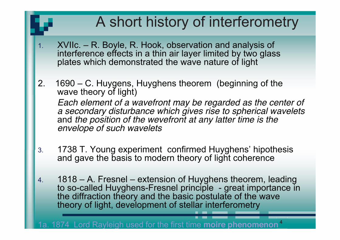
A short history of interferometry 1. XVIIc. R. Boyle, R. Hook, observation and analysis of
interference effects in a thin air layer limited by two glass plates which demonstrated the wave nature of light
2. 1690 C. Huygens, Huyghens theorem (beginning of the
wave theory of light) Each element of a wavefront may be regarded as the center of
a secondary disturbance which gives rise to spherical wavelets and the position of the wevefront at any latter time is the envelope of such wavelets
3. 1738 T. Young experiment confirmed Huyghens hipothesis
and gave the basis to modern theory of light coherence 4. 1818 A. Fresnel extension of Huyghens theorem, leading
to so-called Huyghens-Fresnel principle - great importance in the diffraction theory and the basic postulate of the wave theory of light, development of stellar interferometry
1a. 1874 Lord Rayleigh used for the first time moire phenomenon
5
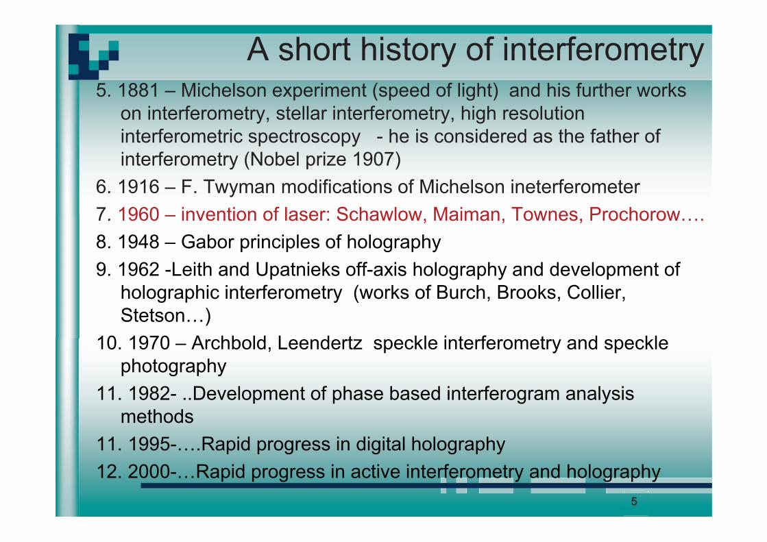
A short history of interferometry 5. 1881 Michelson experiment (speed of light) and his further works
on interferometry, stellar interferometry, high resolution interferometric spectroscopy - he is considered as the father of interferometry (Nobel prize 1907)
6. 1916 F. Twyman modifications of Michelson ineterferometer 7. 1960 invention of laser: Schawlow, Maiman, Townes, Prochorow 8. 1948 Gabor principles of holography 9. 1962 -Leith and Upatnieks off-axis holography and development of
holographic interferometry (works of Burch, Brooks, Collier,
10. 1970 Archbold, Leendertz speckle interferometry and speckle photography
11. 1982- ..Development of phase based interferogram analysis methods
11. 1995- Rapid progress in digital holography 12. 2000- Rapid progress in active interferometry and holography

6
Fundamentals of interferometry
triexpEt,rE iii0i
1,2i;t,rEt,rEi
i
2*1
*21
*22
*11
*
2121
2
21
2EEEEEEEEEEEEEEE I(r)
ttrrcosII2IIIII)rI( 212121211221
Resultant vector in two beam interferometry
i
*22
Result of two beam interference (E field intensity):
Conditions for stationary interference field:
.constrr 21
21Recommended: parallel polarization of beams
Vector of electric field

7
Fundamentals of interferometry
For 1= 2 (usually one source applied)
r cos r1~r cos rbrarr cosII2II)rI( 212121
2
1
Re
E20
E10 Im
rrr 21
is phase difference between the interfering beams
Where a(r) and b(r) are background and fringe modulation functions
21
21
IIII2
is contrast of interferogram
Graphic representation of interf. E vectors
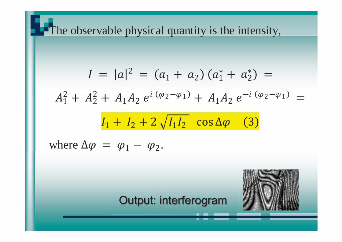
The observable physical quantity is the intensity,
where .
Output: interferogram
9
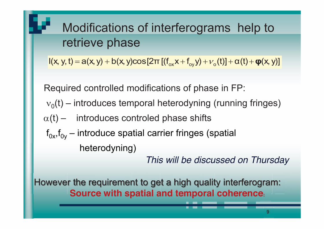
Modifications of interferograms help to retrieve phase
Required controlled modifications of phase in FP: 0(t) introduces temporal heterodyning (running fringes)
(t) introduces controled phase shifts f0x,f0y introduce spatial carrier fringes (spatial heterodyning)
y)](x,(t)(t)]y)fx[(f y)cos[2b(x, y)a(x,t)y,I(x, ooyox
This will be discussed on Thursday
However the requirement to get a high quality interferogram: Source with spatial and temporal coherence:

nterferometer to determine the coherence length of a laser source
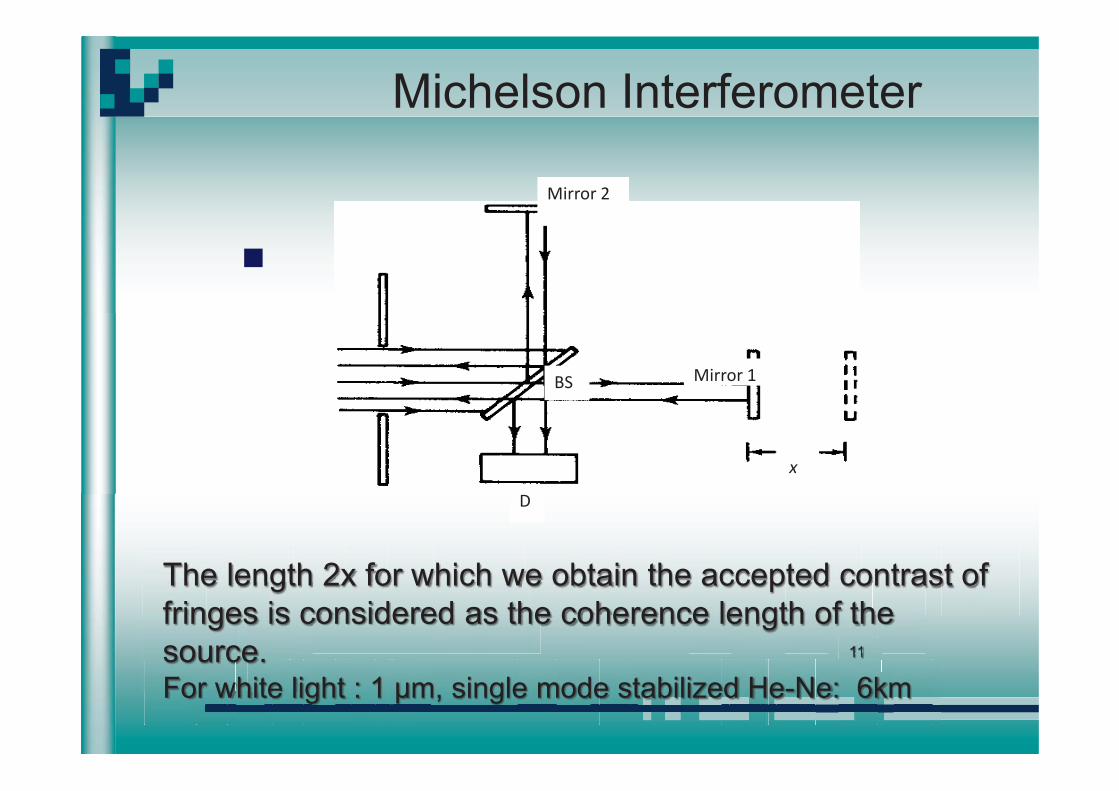
Michelson Interferometer
11
11
The length 2x for which we obtain the accepted contrast of fringes is considered as the coherence length of the source. For white light : 1 m, single mode stabilized He-Ne: 6km
3. Useful Interferometers
Amplitude and Wavefront Divisiontypes (only a few)
Light waves can interfere only if they are emitted by the samesource

Interferometers
Light Source
Wavefront divider
Phase (optical path) difference
Wavefront combiner
Interference

Wavefront Division

T. Young (1801)
D
P1
P2
S1
S2 z
y
x
P1
P2
D
2d

if , then
On substituting into eq (3)
This equation represents a fringe pattern parallel to the y axis, with period
.
The Thomas Young interferometer is being used in FEL to measure its coherence!

measure star diameters.
Other types of wavefront division interferometer are:
- Fresnel biprism
-
- Michelson stellar
Amplitude Division

Michelson Interferometer
19

if mirror M2 is translated a distance x, the optical path difference with respect to mirror M1 is 2x, thus
That gives a total intensity on the detector,

As the mirror 2 is translated a certain distance d, and by counting the number of maxima (bright fringe) per unit time it is possible to measure the speed of an object.
The Michelson Interferometer used with a low coherence source gives way to: low coherence reflectometry, LCR, and Optical Coherence Tomography, OCT. Study of semitransparent materials, biological tissues!
Other good examples of amplitude dividing interferometers are:
- Mach-Zehnderarms (as proposed by Prof. Mataloni)!; Microchannel fabrication (Prof. Ramponi)
- Twyman-Green
-

Challanges for interferometry Example: M(O)EMS Characterisation
vibration (time averagelaser interferometry)
topography - inner structure optical coherence tomography
deformation (laser interferometry) )) asaslala
dimensions/shape (white light interferometry)
© Veeco
and many more ...
( iti© Femto-ST
totoooottooo
topography (digital holography) topograppphh© Lyncèe Tec
© SINTEF © Heliotis
© SINTEF

Main challenge in M(O)EMS inspection
Wafer size increases current diameters , Up to several thousands structures on one wafer (time issues) Feature size decreases typically <10mm2 Inspection ratio: 10-3 to 10-7 100% M(O)EMS inspection
15cm
700μm

Parallel Inspection concept
illumination unit
camera array
probing wafer
M(O)EMS wafer
parallel approach time and cost efficient multi-functional in-line inspection of:
shape deformation resonance frequencies and mode shape
J. Micromech. Microeng. 22 , 015018 , 2012

Micro optical LCI array
Mirau type

Micro optical LI array
DOE based Twyman Green type

Instrument plattform
© SUSS Test Systems Cascade Microtech
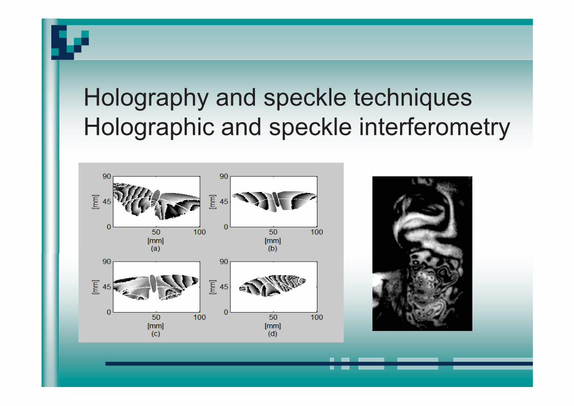
Holography and speckle techniques Holographic and speckle interferometry

30
Registration of optical hologram basic setup
1. Need to have equal optical paths of reference and object beams (within coherence length of laser) 2. During recording the phase between object and reference beams cannot change more than
0.2 < max
Requirements:
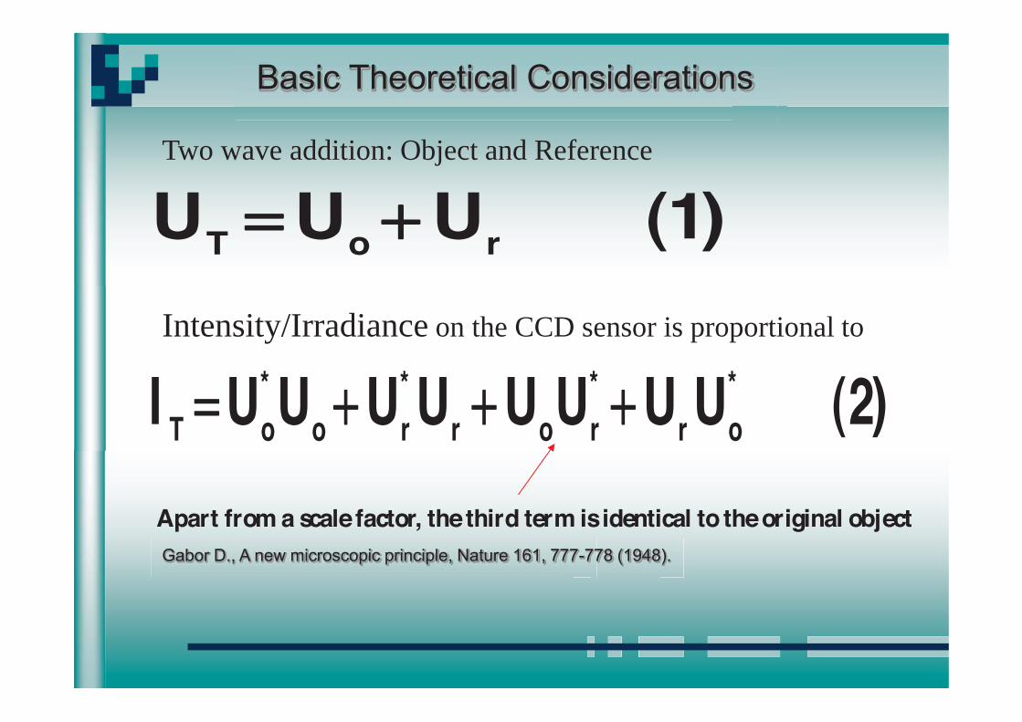
)1(UUU roT
Intensity/Irradiance on the CCD sensor is proportional to
Two wave addition: Object and Reference
)2(UUUUUUUUI *or
*ror
*ro
*oT
Apart from a scale factor, the third term is identical to the original object
Basic Theoretical Considerations
Gabor D., A new microscopic principle, Nature 161, 777-778 (1948).

32
Registration of digital hologram
Photographic (analog) material is replaced by CCD or CMOS matrix
33
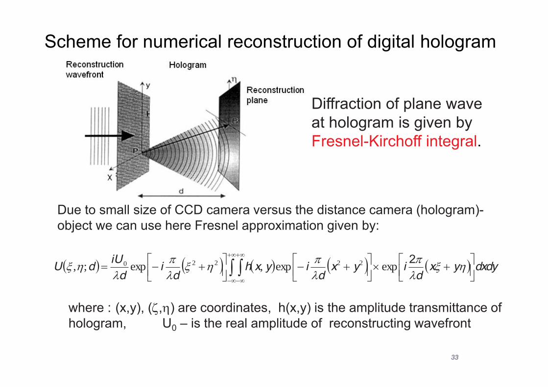
Scheme for numerical reconstruction of digital hologram
dxdyyxd
iyxd
iyxhd
id
iUdU
2expexp,exp;, 22220
where : (x,y), ( , ) are coordinates, h(x,y) is the amplitude transmittance of hologram, U0 is the real amplitude of reconstructing wavefront
Due to small size of CCD camera versus the distance camera (hologram)-object we can use here Fresnel approximation given by:
Diffraction of plane wave at hologram is given by Fresnel-Kirchoff integral.
34
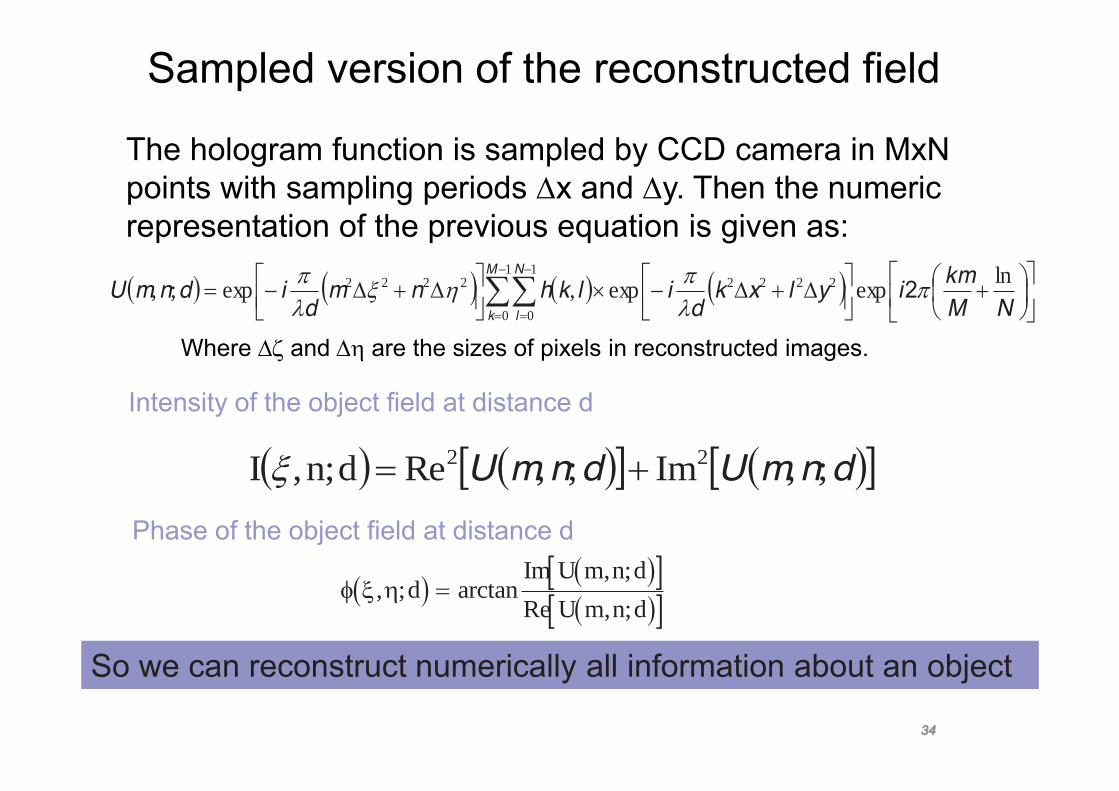
Sampled version of the reconstructed field
NMkm
iylxkd
ilkhnmd
idnmUM
k
N
l
lnexpexp,exp;,1
0
1
0
22222222 2
dnmUdnmU ;,Im;,Redn;,I 22
, ; arctanIm , ;Re , ;
dU m n dU m n d
Intensity of the object field at distance d
Phase of the object field at distance d
The hologram function is sampled by CCD camera in MxN points with sampling periods x and y. Then the numeric representation of the previous equation is given as:
Where and are the sizes of pixels in reconstructed images.
So we can reconstruct numerically all information about an object
35
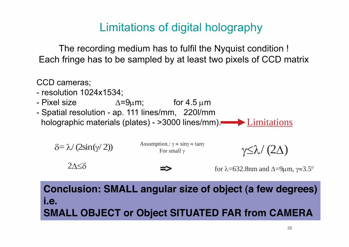
Limitations of digital holography
CCD cameras; - resolution 1024x1534; - Pixel size =9 m; for 4.5 m - Spatial resolution - ap. 111 lines/mm, 220l/mm holographic materials (plates) - >3000 lines/mm). Limitations
The recording medium has to fulfil the Nyquist condition ! Each fringe has to be sampled by at least two pixels of CCD matrix
= / (2sin( / 2))
2
/ (2 )=> for =632.8nm and =9 m, 3.5
Assumption.: sin tan For small
Conclusion: SMALL angular size of object (a few degrees) i.e. SMALL OBJECT or Object SITUATED FAR from CAMERA

Reference beam
Single mode optical fiber
IL
A
BC
CCD
Object beam
Reference beam
cw/Pulsed Laser Object beam
4. ESPI/TV H set-up
PC, and Monitor
Moving object

37
HOLOGRAPHIC INTERFEROMETRY
- Classical - Digital
C. M. Vest, Holographic interferometry, J. Wiley and Sons, New York, 1979 P. K. Rastogi (ed), Holographic interferometry, Springer, 1994 I. Yamaguchi, T. Zhang, Phase shifting digital holography, Opt. Lett., 22, 1268-1270, 1997 T. Kreis -VCH Verlag GmbH & Co.KGaA, 2005

38
Classical holographic interferometry
Piexp PAPE p1p1
PPiexp PAPE p2p2
Each holographic system can be used to compare optical wavefronts formed by an object in different states (physical conditions)
Let initial state of an object is:
After providing load (or other changes)
If the object (load) is stationary we may compare these wavefronts by: -double exposure holographic interferometry,-real time holographic interferometry.
If the object is vibrating we use: -Time averaged holographic interferometry -Stroboscopic holographic interferometry
In the case of dynamic object investigation we use impulse double exposure HI
39
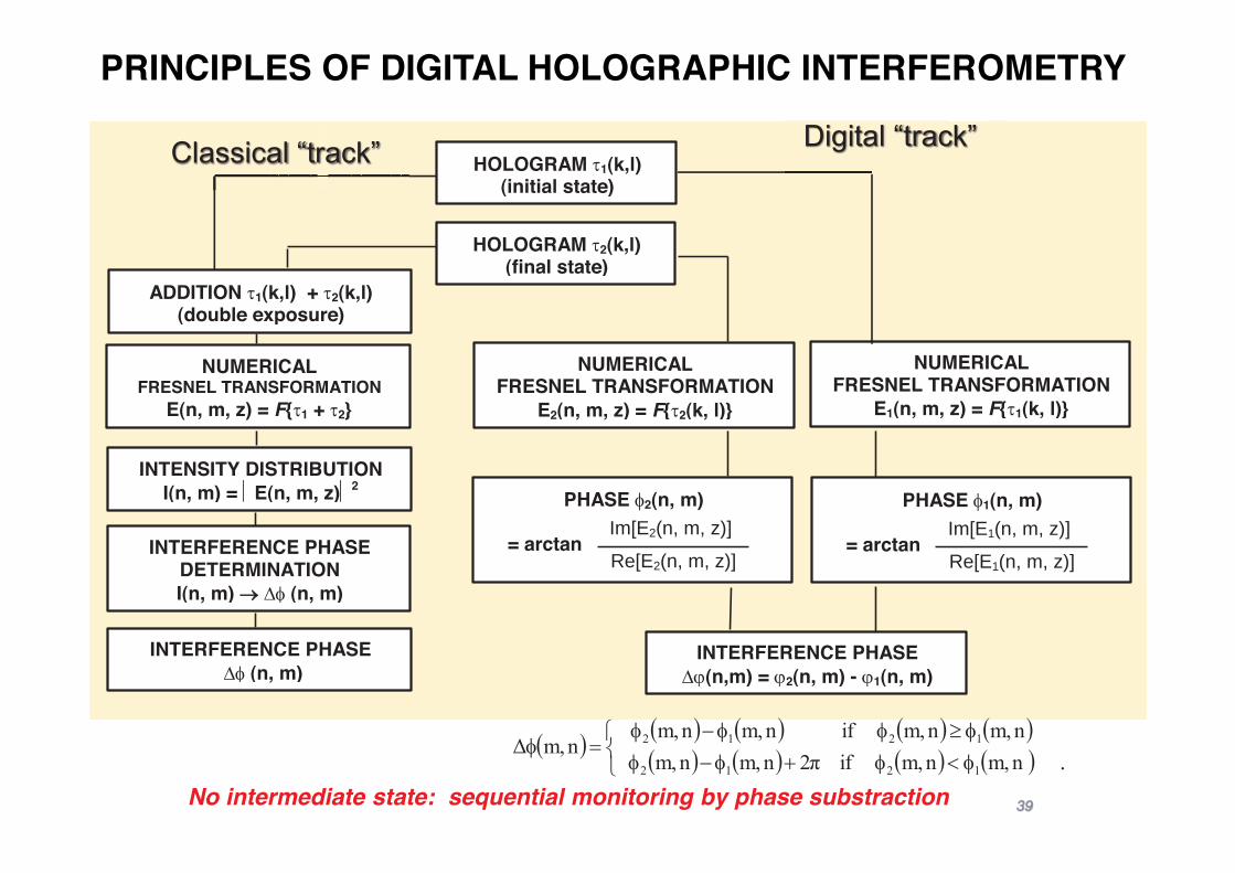
PRINCIPLES OF DIGITAL HOLOGRAPHIC INTERFEROMETRY
HOLOGRAM 1(k,l) (initial state)
HOLOGRAM 2(k,l) (final state)
INTERFERENCE PHASE (n,m) = 2(n, m) - 1(n, m)
ADDITION 1(k,l) + 2(k,l) (double exposure)
INTERFERENCE PHASE DETERMINATION I(n, m) (n, m)
INTENSITY DISTRIBUTION I(n, m) = E(n, m, z) 2
NUMERICAL FRESNEL TRANSFORMATION
E(n, m, z) = F{ 1 + 2}
INTERFERENCE PHASE (n, m)
NUMERICAL FRESNEL TRANSFORMATION
E2(n, m, z) = F{ 2(k, l)}
NUMERICAL FRESNEL TRANSFORMATION
E1(n, m, z) = F{ 1(k, l)}
PHASE 2(n, m)
= arctan
Im[E2(n, m, z)]
Re[E2(n, m, z)]
PHASE 1(n, m)
= arctan
Im[E1(n, m, z)]
Re[E1(n, m, z)]
No intermediate state: sequential monitoring by phase substraction
.
Classical track track
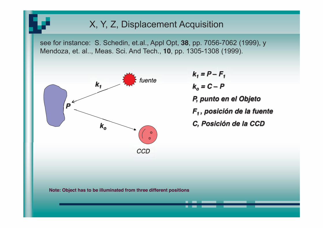
X, Y, Z, Displacement Acquisition
see for instance: S. Schedin, et.al., Appl Opt, 38, pp. 7056-7062 (1999), y Mendoza, et. al.., Meas. Sci. And Tech., 10, pp. 1305-1308 (1999).
P
k1
ko
k1 = P F1
ko = C P
P, punto en el Objeto
F1 , posición de la fuente
C, Posición de la CCD
fuente
CCD
Note: Object has to be illuminated from three different positions
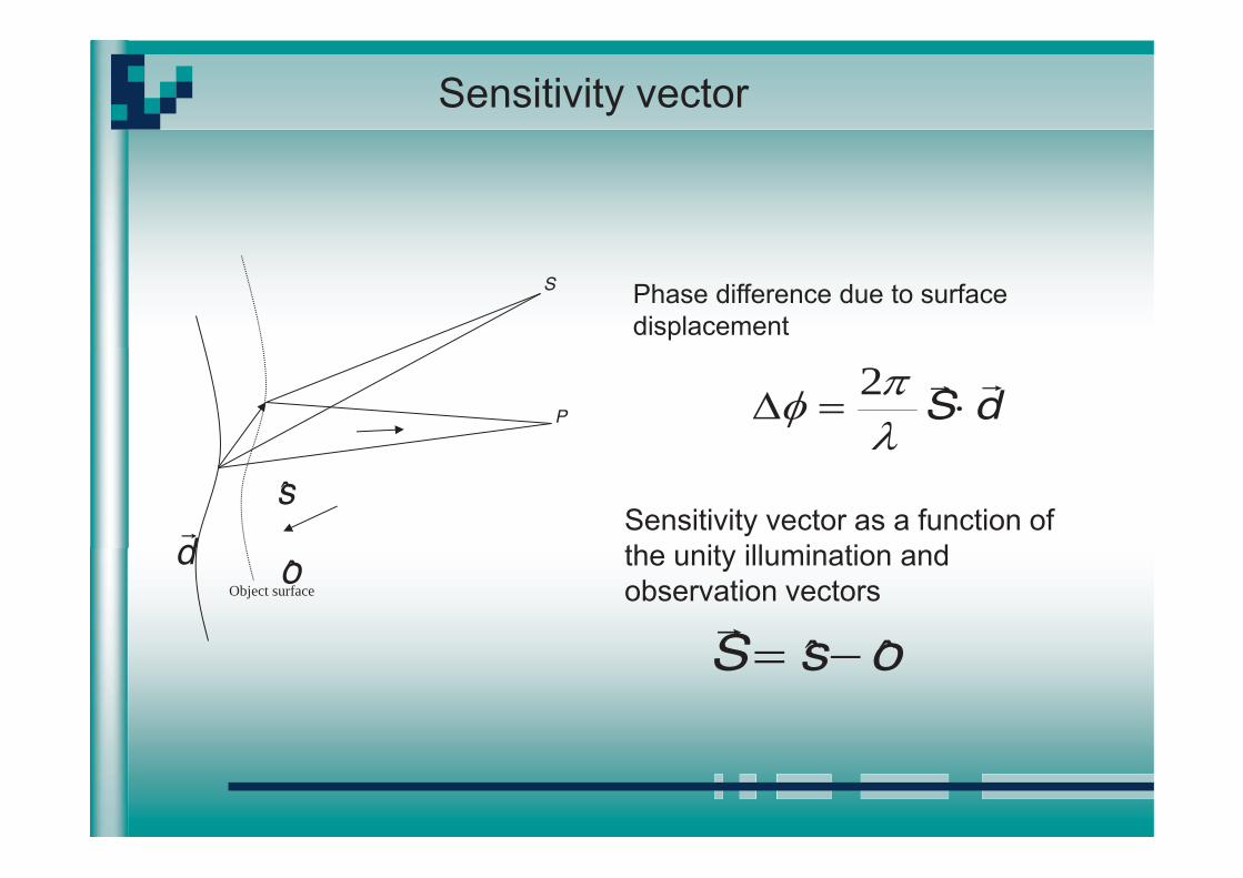
Sensitivity vector
dSensitivity vector as a function of the unity illumination and observation vectors
osS
dS2
Phase difference due to surface displacement
Object surface
P
S
s
o

2D measurements (an in plane and an out of plane component)
Out of plane displacements
Z
X
In plane displacements
1s
2s
o
2D evaluation requires two independent sensitivity vectors
)cos1,sin(1S
)cos1,(sin2S
Sensitivity vectors
1S
2S
zSSS 21
1S 2S
From equation (7)
zz Sd2
12 (9)
1S
2SxSSS 21
Out of pane sensitivity
In plane sensitivity
xx Sd2
12 (10)
(11) 2
11
cos1cos1
2 sen
sen
d
d
z
xFrom eq. (7)

3D Sensitivity
3D evaluation requires three sensitivity vectors
Deformation components are evaluated at each point of the
3
2
11
cos10sincos1sin0cos10sin
2z
y
x
d
d
d(12)
2s
3s
1s
Y
Z
X
2S
1S
3S

The displacement information must now be drawn on the Object Contour (shape), which may be found using any of several different/complementary (optical and non-optical) techniques, viz., Pedrini, et. al., App Opt, 38, pp. 3460-3467 (1999) Rodriguez, et. al. JOSA, A 9, pp. 2000-2008 (1992)

RESULTS

ESPI A) Underwater Sonar at 3KHz B) Traveling wave C) In-plane harmonic oscillation at 33 and
37 KHz

Journal of Sound and Vibration, 172 (4), pp. 433-448 (1994).


Applied Optics, 30 (7), pp. 717-721 (1991).
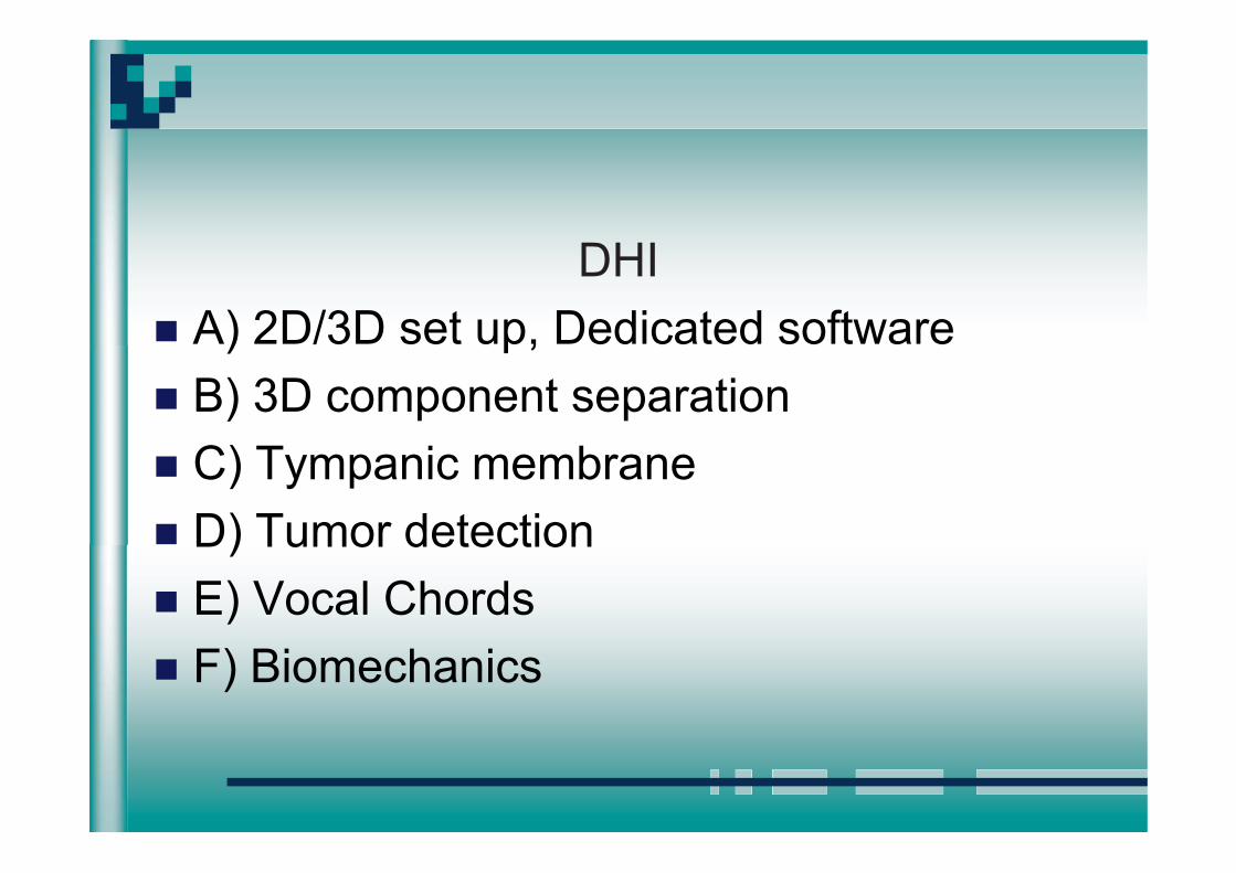
DHI A) 2D/3D set up, Dedicated software B) 3D component separation C) Tympanic membrane D) Tumor detection E) Vocal Chords F) Biomechanics

Laser M1
Load
Object
P1 P2
P3
OF1
OF2
BS
M2
L
A BC CCD
BS
M1
CCD
Object
Laser
BS1 OF
M2
P1
P3
P2 BC
A L Load
BS2
BS3


3
2
11
323
222
111
2zzx
yyx
zyx
z
y
x
SSS
SSS
SSS
d
d
d
Phase evaluation with 3 holograms

Separation of individual displacement components


OH
IP
FSFO
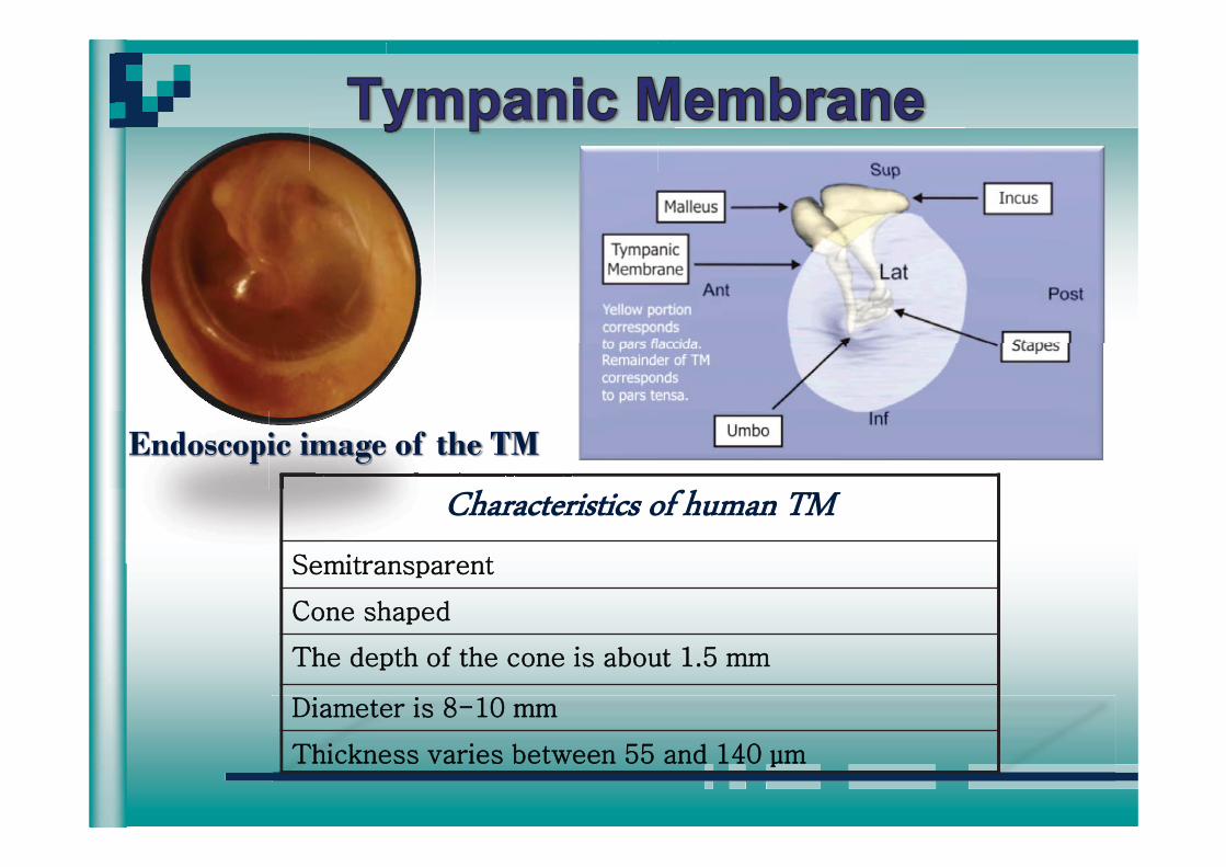
TM
OBOOO
RB

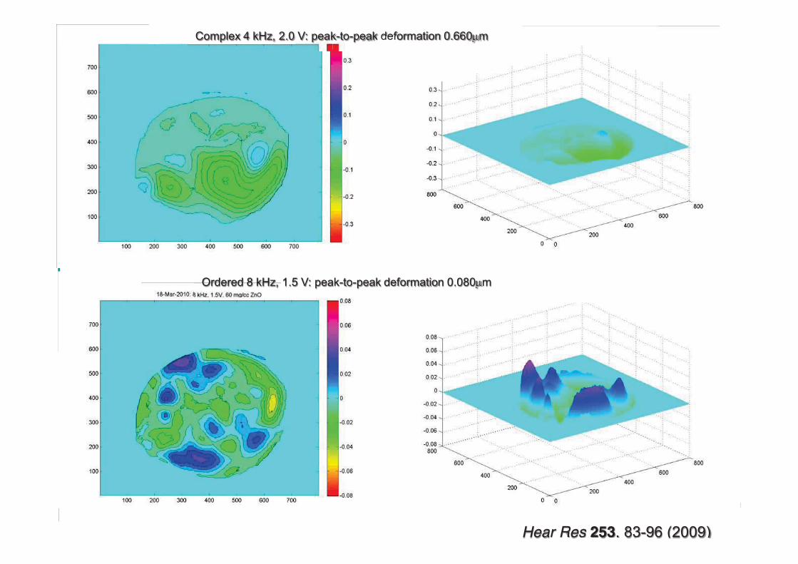
Hear Res 253, 83-96 (2009)
Complex 4 kHz, 2.0 V: peak-to-peak deformation 0.660 m
Ordered 8 kHz, 1.5 V: peak-to-peak deformation 0.080 m

noisy?

softer classical

2 2 2

Shown : Tympanic annulus and handle of maleus

3D Displacement on the TM shape

3D Displacement on the TM shape

INHOMOGENEITIES DETECTION (TUMORS)
Input sound power of approximately 661 mW, equivalent to a pressure of 2.3 x 10⁵ pa. Laser pulse separation 14 ms, at 532 nm, 15 ns pulse width, 20 mJ/pulse, average power of 0.639 W/cm2 at the surface, and 6 m of coherence length. CCD with 1024 by 1280 pixels at 12 bits. Phantom is a semi sphere with an 8.4 cm in diameter and 4 cm height.
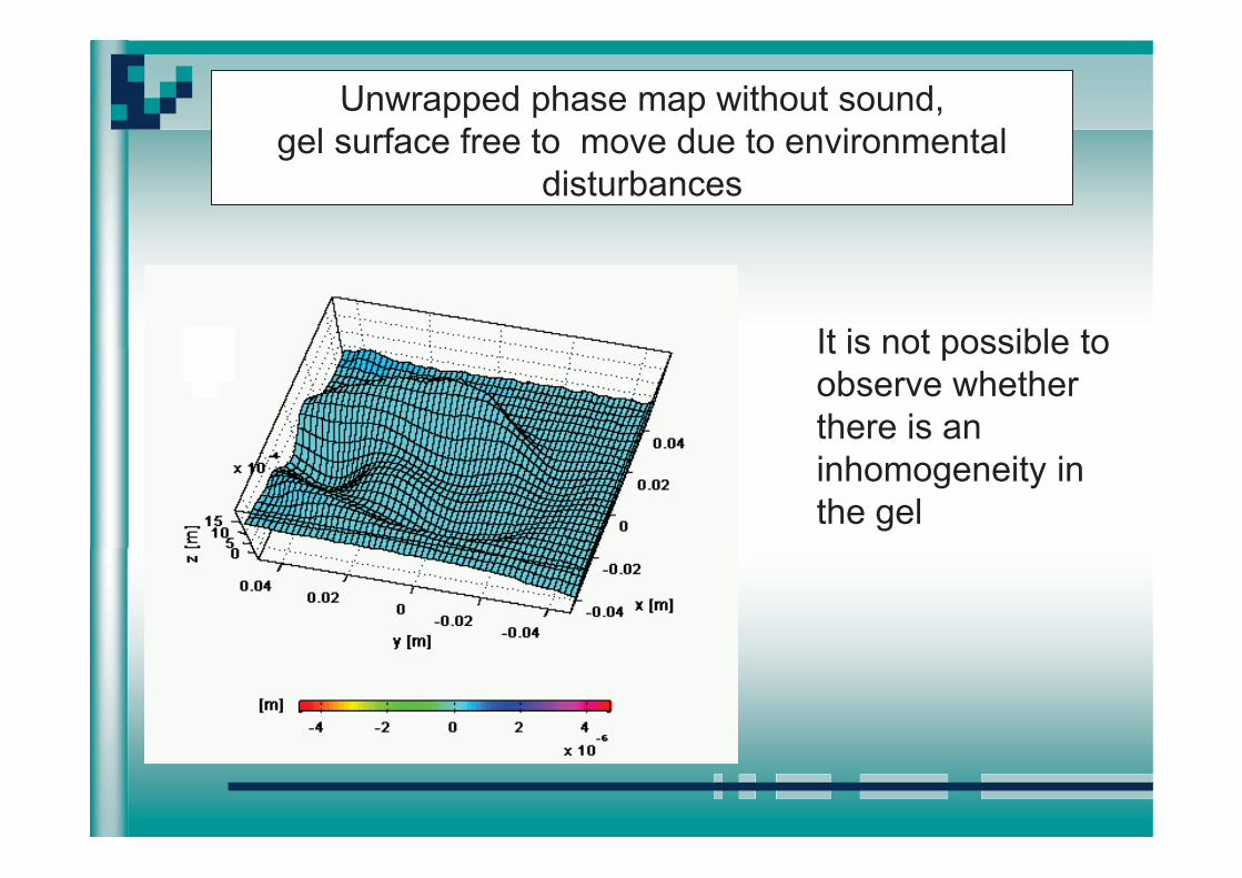
Unwrapped phase map without sound, gel surface free to move due to environmental
disturbances
It is not possible to observe whether there is an inhomogeneity in the gel
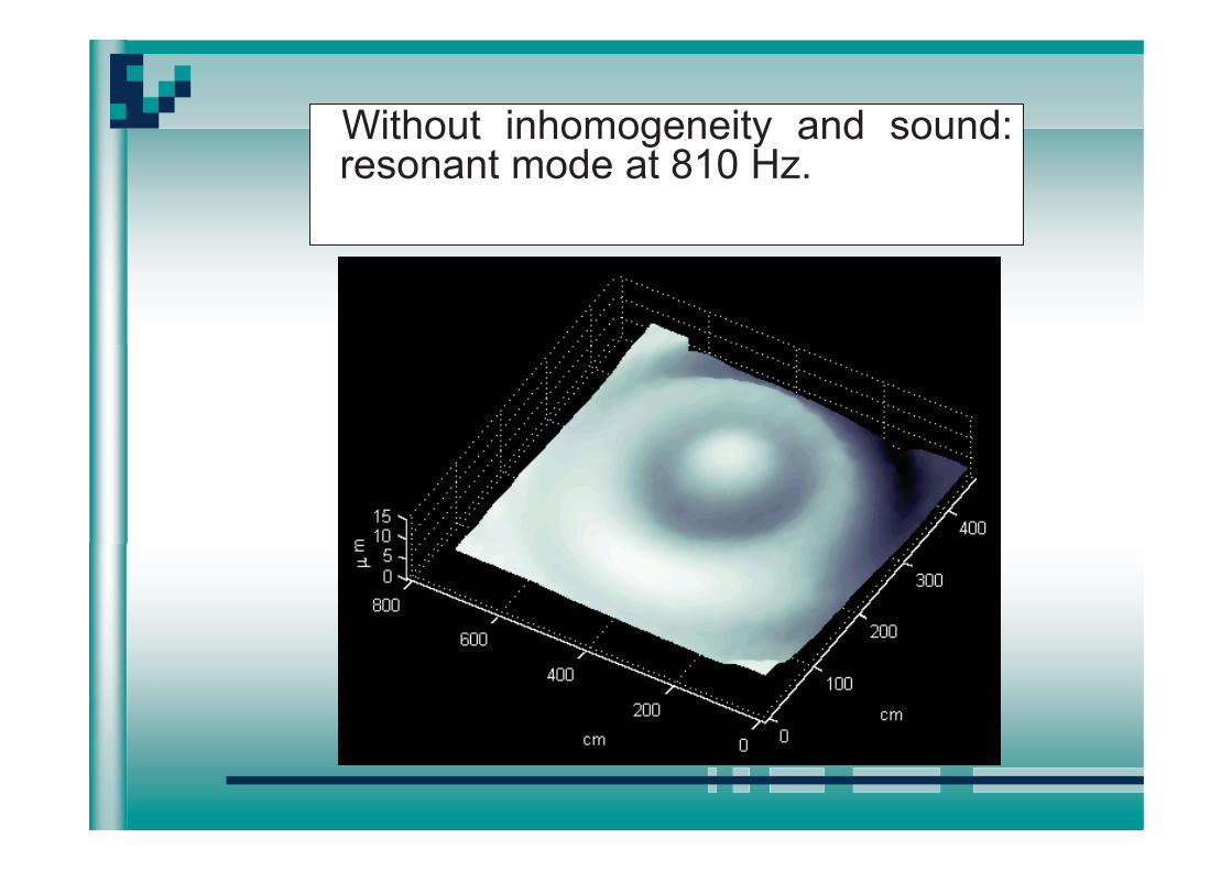
Without inhomogeneity and sound: resonant mode at 810 Hz.
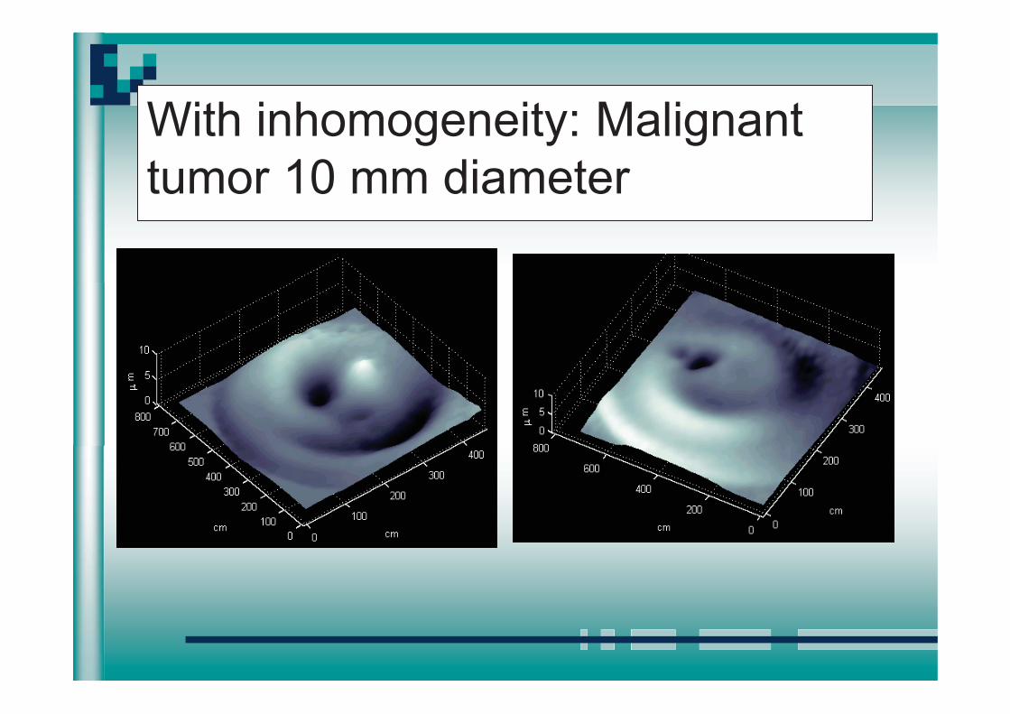
With inhomogeneity: Malignant tumor 10 mm diameter

Unwrapped phase maps corresponding to each illumination direction
L
C
R
With 3D data the depth of the tumor may be found

Malignant tumor 10 mm diameter, 3D data
Journal of Biomedical Optics, 12 (2), pp. 024027-1/024027-5 (2007).

Depth location with respect to the surface
- 1. 0 8 E- 0 6
- 1. 13 E- 0 6-1.20E-06
-1.00E-06
-8.00E-07
-6.00E-07
-4.00E-07
-2.00E-07
0.00E+00
0 7 14 21 28 35 42 49 56 63 70 77 84
surface length
surf
ace
disp
lace
men
t

Results fitted to a straight line for calibration purposes

2000 fps
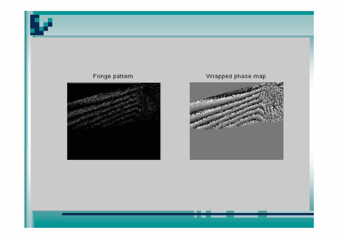
FRINGE PATTERN
WRAPPED PHASE
Vocal chords displacements ( Larinx)
VOCAL CHORDS MOVEMENT
La amplitudes de vibración y las velocidades depende de la fonación. Así como la edad y sexo, determinan sus características fisiológicas de las cuerdas.

FRINGE PATTERN WRAPPED PHASE
2000 fps
VOCAL CHORDS MOTION
1)BS1
2) 3)
BS2
OF1 BS3
BC1
L A
M1
M4
M2 M3
M5
OF3 OF2
Object
CMOS
NDF1
NDF2
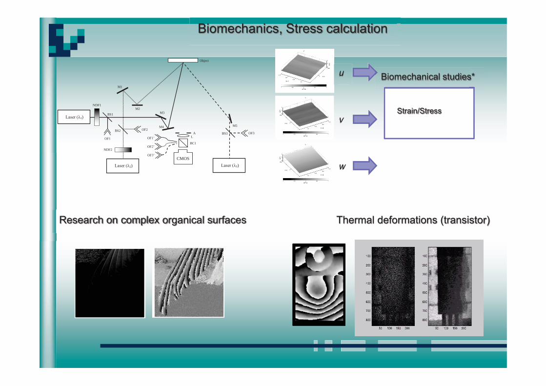
Research on complex organical surfaces
Biomechanics, Stress calculation
Thermal deformations (transistor)
u
v
w
Strain/Stress
Biomechanical studies*

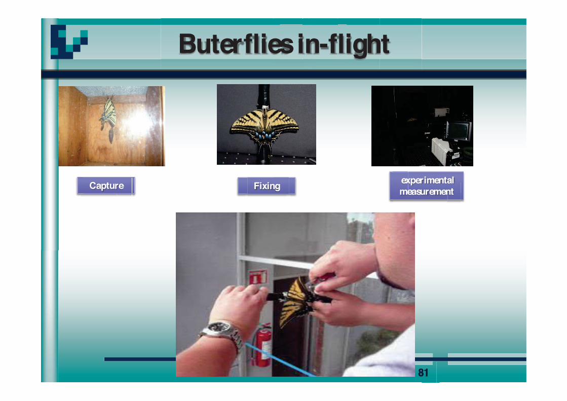
Buterflies in-flight
81
Capture Fixing experimental measurement

82
Comparison among 4 butterflies
in-vivo experimentation High speed DHI Laser Verdi (Coherent V6) Ilumination density on the insecto:
19.6 mW/cm2
NAC GX-1 camera Recordings at 4000 fps FOV: 90 x 100 mm 800 x 800 pixeles 10 bits dynamic range
Pterourus Multicaudata
Dannaus Gillipus Cramer
Agraulis Vanillae Incarnata
Precis Evarete Felder

83
Wrapped phase maps
5. Resultados Experimentales

84
Unwrapped phase maps
5. Resultados Experimentales


Summary
-Interferometry
- Interferometry allows the non contact more accurate measurements known today. Novel approaches are all the time on the way - Interferometric systems are being used in many areas of Optics and Photonics, from optical shop testing to writing of Bragg gratings, to being incorporated in lab in a chip. Electronic Speckle Pattern Interferometry have been successfully used over the last 40 years. - Digital Holographic Interferometry brought solutions to new challenges
ACKNOWLEDGEMENTS
MY DEEPEST APPRECIATION TO ICTP FOR HAVING INVITED ME TO CO-DIRECT THIS
samebut as a STUDENT!!

Thank you for your kind attention