[1]

Introduction

Interferometry is a method of experiment in which electromagnetic waves are made to interfere so that their properties may be observed. Considering physics in particular, it enables scientists to measure small displacements of systems, determine changes in refractive indices; and even to analyse the mechanical stress-strain properties of substances - to name a few. With its numerous applications in disciplines ranging from the vast field of astronomy down to the infinite well of quantum mechanics; as well as in aspects of molecular biology and chemistry; interferometry is indeed one of the most important investigative techniques known to modern science.

In this 3-part experiment, we initially construct a particular type of light wave interference system, known as the Michelson Interferometer, and then use it to measure the magnetostrictive effect, of an applied magnetic field, on a set of two ferromagnetic metal samples and copper. Lastly, the interferometer setup will be modified in order to measure the refractive index of air.

Abstract

Part 1 Constructing the Michelson Interferometer

In order to measure the magnetostriction of metals, a Michelson interferometer is constructed on a magnetic optical base plate that has a grid inked on its surface for ease of component placement. The interferometer consists of 4 identical mirrors, a lens, a coil with the metal samples in the form of cylindrical rods, a half-silvered beam splitter and a detecting screen onto which the fringe pattern is projected.

Part 2

Measuring the magnetostriction of different metal samples

Using the interferometer constructed in Part 1, the behaviour of the metal samples under the effect of a varying magnetic field is observed. It is found that, due to magnetostriction, the iron sample initially lengthens and then contracts, whereas the nickel sample contracts only. Copper, being non-ferromagnetic, experiences no change in dimensions while under the effect of the magnetic field.

Part 3

Measuring the refractive index of air

The interferometer setup for measuring magnetostriction is modified (with the addition of a cuvette connected to an air extraction pump in one of the arms of the interferometer) to measure the change in refractive index of the air within the cuvette. This is done by observing the fringe changes on the detecting screen as the pressure in the cuvette is varied. The calculated value of the refractive index of air, 𝑛𝑎𝑖𝑟 was found to be 1.000296 ±0.000012, which is very close to the literary value (at normal pressure and temperature): 𝑛𝑎𝑖𝑟 = 1.000269.

Michelson Interferometry

Hassan Mirza Queen Mary University, Department of Physics

Mile End Road, London, England, E1 4NS

[2]

Part 1 Constructing the Michelson

Interferometer

I. Objective

To build a Michelson interferometer for

measuring the magnetostriction of metal samples.

II. Basic Theory

Electromagnetic waves can interfere in two

ways: by (a) division of amplitude and (b) division

of wavefront.

In the Michelson interferometer, light is

split into two separate beams via division of

amplitude. This is achieved by the placement of a

half-silvered glass plate, at an angle of 45o, to the

direction of the incident light. Both beams are then

reflected by mirrors and brought to interference –

the pattern of which is observed on a screen placed

behind the half-silvered plate. See Figure 1 for

details.

III. Setup Procedure

The interferometer to be constructed in this

experiment operates using a red laser of

wavelength 𝜆 = 632.8 nm as the main light source.

The entire system is set up on a magnetic optical

base plate that has an 𝑥- and 𝑦- coordinate grid

inked on its surface. This allows the separate

components, all of which have magnetic bases, to

be placed in their respective positions accurately

and ensures that they do not move unintentionally.

The position of each component will be referred to

by the 2-tuple [𝑥,𝑦] describing its coordinates on

the axes of the base plate.

Below are the steps that yield the

interferometer setup shown in Figure 1 and Figure

2 upon completion. The data amassed while

carrying out the steps, with errors, are also given.

This is the same setup that will be used in Part 2 to

measure the magnetostriction of different metals:

1. Carefully place the laser emitter on the

base plate so that its centre is

approximately positioned at [6,8] with

the laser traveling in the correct

direction. The exact horizontal

placement of the laser is not relevant.

2. Place the screen SC at [6,6] on the base

plate.

3. Check the height (of the laser beam’s

point of emission) above the surface of

the base plate. This is measured to

be 135 ± 5 mm.

4. The first mirror M1 is placed at [1,8] on

the base plate. Its height is adjusted so

that the centre of the mirror is 135 ±

5 mm high.

5. Adjust the angle of M1 until its plane is

approximately 45o to the line of traverse

of the incident laser light. This is

checked by observing how closely the

light reflected from M1 lines up with

the line 𝑥 = 1 on the base plate.

6. The second mirror M2 is placed at the

position [1,4] with its plane being at

approximately 45o to the light reflected

from M1 and the height of its centre at

135 ± 5 mm . The required angle can

be set by observing how closely the

light reflected from it lines up with the

line 𝑦 = 4 on the base plate, and

Figure 1: Michelson interferometer setup for

measuring magnetostriction of metals.

C C

Nickel rod

[3]

adjusting it accordingly until they line

up as close as possible.

7. Next, the third mirror M3 is screwed

into place at the end of the nickel rod.

Nickel will be the one of the metal

samples to be tested for

magnetostriction in the next part of the

experiment.

8. The nickel rod, together with the

attached mirror M3, is inserted inside

the coil C as shown in Figure 1. The

rod’s axes should align centrally with

that of the coil so that the rod extends

beyond both ends of the coil by an

equal distance. This justifies the

assumption that the magnetisation is

uniform across the length of the metal

sample. The distance extended at both

ends is measured to be 30 ± 1 mm.

9. The combined fixture of the coil C,

nickel rod and M3 is placed at [11,4]

on the base plate with the plane of M3

being perpendicular to the laser light

reflected from M2 and the height of its

centre being 135 ± 5 mm. This step is

complete once M3 is adjusted in a way

that the light reflected from it strikes its

point of origin on M2 – that is, the point

at which the light from M1 strikes the

surface of M2. (Minute adjustments of

the tilt of M1 and M2 can be made

using the fine adjustment screws on the

back of the mirrors.)

10. The half-silvered beam splitter glass BS

is place at [6,4] on the base plate. It is

rotated so that the light from M2 strikes

the metallic side, while that from M3

strikes its glass side; both at 45o. This

can be accomplished by observing how

closely the reflected light from BS lines

up with the line 𝑥 = 6 on the base plate,

and adjusting its rotation until they line

up as close as possible. Note that the

transmitted light from BS should reach

M3 without hindrance.

11. Once BS is in the correct position, the

fourth and final mirror M4 is placed at

[6,1] so that its plane is struck by the

light reflected from the metallic side of

BS and that the height of its centre

is 135 ± 5 mm. There should now be

two distinct spots visible on the screen

SC.

12. Adjust M4 using its fine adjustment

screws so that the two distinct spots on

SC overlap and merge. A slight

flickering of the combined spot is

observed.

13. Finally, the lens L is placed at [1,7].

The position of L is adjusted until an

interference pattern is observed on the

screen SC.

14. Readjust M4 using its fine adjustment

screws once again until there are

concentric-circular interference fringes

clearly visible on the screen SC. The

interferometer setup is now complete.

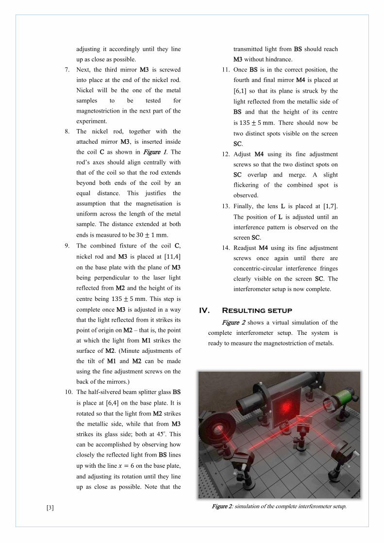
IV. Resulting setup

Figure 2 shows a virtual simulation of the

complete interferometer setup. The system is

ready to measure the magnetostriction of metals.

Figure 2: simulation of the complete interferometer setup.

[4]

Part 2 Measuring the magnetostriction

of different metal samples

I. Objective

To use the interferometer constructed

previously for measuring the magnetostriction of

nickel and iron samples. The results are to be

plotted on a graph and compared with the one

given in literature. A copper sample will also be

tested.

II. Basic Theory

Magnetostriction Magnetostriction is a property specific to

ferromagnetic substances. It causes them to change

shape slightly when under the effect of an applied

magnetic field. This is due to the fact that

ferromagnetic materials consist of separate regions

within their structures that have uniform

magnetisation – i.e. the magnetic dipoles of

molecules in these regions are unidirectional. These

regions are known as domains.

When an external magnetic field is applied,

the magnetisations of the domains also change. The

domains themselves do not change shape since they

are held tightly within the crystal structure of the

metal. It is the realignment of the magnetic dipoles

in the domains, in response to the applied magnetic

field, which gives rise to magnetostriction.

Magnetic field strength of a coil The system setup in previously for

measuring magnetostriction consists of the metal

sample placed inside a cylindrical coil, as shown in

Figure 1 and Figure 2. The magnetic field strength

at the centre of such a coil is given by

The terms in this expression are defined below. The

corresponding quantities specific to the experiment

apparatus of Part 1 are also given in brackets:

𝐻𝑚 = magnetic field strength at the centre of the

coil (measured in ampere per metre, Am−1).

𝑁 = the number of windings in the coil (1200)

𝑟 = radius of winding (0.024 m)

𝑙𝑐 = length of the coil (0.06 m)

𝑁 = the magnitude of DC current supplied to the

coil.

The expression in (1) can simplified

significantly using the assumptions that (a) the field

is uniform (as stated in Part 1), and (b) that the field

strength at the centre of the coil, 𝐻𝑚, acts on the

entire length of the rod, 𝑙 = 0.15 m. We also note

and make use of the constraint that 𝑙 ≫ 𝑟. Thus,

by taking these into consideration and replacing 𝑙𝑐

with 𝑙 in (1), the obtained equation is

which gives the magnetic field strength acting

across the entire length of the metal rod sample.

Interference fringes and alteration lengths Consider the interferometer constructed in

Part 1. If DC voltage and current are supplied to

the coil, holding the voltage constant while varying

the current will cause changes in the interference

pattern observed on the detecting screen – the

circular fringes move outward radially (source)

and/or move inward radially (sink).

Suppose now that a given change in the

supplied current causes a new circular fringe to

source from the centre of the interference pattern

on the screen (𝑛 = 1); and that another change in

supplied current causes a second fringe to source

(𝑛 = 2), and so on. Using this change, labelled

as 𝑛, together with the fact that the separation of

two adjacent circular fringes on the screen is half

the wavelength of the laser light, 𝜆2, the change of

𝐻𝑚 =𝑁𝑁

�4𝑟2 + 𝑙𝑐2.

𝐻 =𝑁𝑁𝑙

; (2)

(1)

[5]

length that the metal sample undergoes as a result

of the applied magnetic field – its alteration length

– may be quantified as

Note that this equation also holds if a change in

current causes the fringe pattern to sink rather than

source; as 𝑛 is measured the same way but will

change sign.

III. Measurement Procedure

The interferometer constructed in Part 1 will

now be used to measure the magnetostriction of

two ferromagnetic samples: nickel and iron.

Copper, although non-ferromagnetic, will also be

tested to observe the functioning of the

interferometer. The setup is used to measure

magnetostriction as follows:

1. If not done so already, carry out steps 7,

8 and 9 outlined on page 2, Part 1 using

the desired metal sample.

2. Connect a power supply to the coil C.

3. The magnetic substances require

premagnetisation before taking

measurements. This is achieved by

increasing and decreasing the current a

few times before performing each

measurement.

4. The current supplied to the coil is

steadily increased until a fringe change

at the centre of the screen is observed.

The fringe change that needs to be seen

corresponds to one complete

wavelength. For example, if the centre

is initially bright, the value of current is

taken after the bright fringe disappears

and another one of approximately the

same size appears. This is one

wavelength change. The choice of

measuring fringe changes from the

centre of the pattern on SC is arbitrary;

but it was found to be easiest this way.

5. Using the convention that sourcing is

positive and sinking is negative, record

and tabulate the fringe change as a

function of applied current for each of

the metal samples.

6. Repeat the measurements twice to

obtain a set of three measurement trials.

7. Calculate, for each measurement, the

alteration length Δ𝑙 using (3), relative

length change Δ𝑙𝑙

, and the magnetic field

𝐻 using (2).

8. Plot a single graph of relative length

change against the magnetic field

strength for nickel and iron.

IV. Results

Following the procedure outlined above, the

measurements that were made are recorded in

Table 1. The corresponding plot is shown below:

-25

-20

-15

-10

-5

0

5

10

0 5 10 15 20 25 30 35

Iron

Nickel

Δ𝑙 =𝑛𝑛2

. (3)

𝐌𝐌𝐌𝐌𝐌𝐌𝐌𝐌 𝐅𝐌𝐌𝐅𝐅 𝐒𝐌𝐒𝐌𝐌𝐌𝐌𝐒 × 103Am−1

Magnetostriction of Iron and Nickel

𝐑𝐌𝐅𝐌𝐌𝐌𝐑𝐌 𝐋𝐌𝐌𝐌𝐌𝐒

𝐂𝐒𝐌𝐌𝐌𝐌

×10

−6

Figure 3: graph of the magnetostriction of iron and nickel. The error bars are scaled by a factor of 20 and the total number of degrees of freedom is 10.

[6]

𝒏 𝑰𝒕𝟏 ± 𝟎.𝟏 𝐀 𝑰𝒕𝟐 ± 𝟎.𝟏 𝐀 𝑰𝒕𝟑 ± 𝟎.𝟏 𝐀 𝑰𝒂𝒗𝒈 ± 𝟎.𝟎𝟑 𝐀 𝚫𝒍 × 𝟏𝟎−𝟕𝒎 𝚫𝒍𝒍 × 𝟏𝟎−𝟔 𝑯 𝐀𝐦−𝟏

IRO

N +1 1.021 1.015 1.010 1.015 +3.12 +2.08 8.12 ± 0.04

+2 2.134 2.146 2.154 2.145 +6.23 +4.15 17.16 ± 0.08 −1 3.418 3.402 3.390 3.403 −3.12 −2.08 27.23 ± 0.12 −2 3.992 4.001 4.010 4.001 −6.23 −4.15 32.01 ± 0.14

NIC

KE

L

−1 0.194 0.190 0.203 0.196 −3.12 −2.08 1.57 ± 0.01 −2 0.289 0.301 0.312 0.301 −6.23 −4.15 2.41 ± 0.01 −3 0.454 0.470 0.491 0.472 −9.35𝐸 −6.23 3.77 ± 0.02 −4 0.612 0.589 0.570 0.590 −12.5 −8.31 4.72 ± 0.02 −5 0.898 0.860 0.856 0.871 −15.6 −10.4 6.97 ± 0.03 −6 1.180 1.301 1.250 1.244 −18.7 −12.5 9.95 ± 0.04 −7 1.672 1.605 1.630 1.636 −21.8 −14.5 13.09 ± 0.06 −8 2.234 2.198 2.240 2.224 −24.9 −16.6 17.79 ± 0.08 −9 3.216 3.230 3.310 3.252 −28.0 −18.7 26.02 ± 0.12

V. Errors and Uncertainties

Quantifying errors

Errors were taken into account while

carrying out step 4 outlined above in III.

Measurement Procedure. The reading of current

given by the apparatus is displayed to 3 decimal

places. However, the errors quoted in Table 1 for

all 3 trials of measurement are to one decimal place

only. This is due to the reading of current

fluctuating significantly on the display; making it

difficult to pinpoint a single value to quote. Thus,

an error was chosen so as to encompass the scale of

fluctuation about the required reading.

Furthermore, if an error of ±0.001 A was quoted,

the propagated error by the end (to the value of 𝐻)

would be negligibly small. The calculated errors

appear in scaled form on the 𝑥-axis of Figure 3

Errors on the quantities that appear on the 𝑦-axis of

Figure 3 are not relevant as they are negligibly

small and would not appear on the graph (as

vertical error bars) without very large scaling.

Uncertainties

The main uncertainty is found to be in the

process of choosing the value of current to quote.

An attempt to minimize the effect of reading

fluctuation was made by taking the value of current

about 5-10 seconds after the fringe change had

been observed. This made no noticeable difference.

While waiting for as little as 10 seconds to make

the measurements, however; it was observed that

the fringe pattern on SC started to change, without

the supplied current being changed. This is likely

due to the coil heating up and altering the

magnetization of the sample undesirably, as it also

heats up and expands. It would indeed destroy the

measurement, and the ones after it, if one was to

wait even longer.

In addition to this, there is also an

uncertainty in determining when exactly one whole

wavelength change occurs in the fringes on SC. To

minimize the effect of this, at the beginning of the

experiment, a small mark is drawn at the edge of

the central fringe on SC. A complete wavelength

change therefore occurs each time this mark is

struck by the edge of a fringe, sourcing or sinking.

VI. References - Queen Mary, Department of Physics. Laboratory

Manual – Experiment 5: Building a Michelson

Interferometer, pages 4-6.

- Joule, James (1842). "On a new class of magnetic

forces". Annals of Electricity, Magnetism, and

Chemistry 8: 219–224

Table 1: the experiment data collected for the magnetostriction of iron and nickel. Copper was also tested the same way. However, as expected, there was no length alteration as it is non-ferromagnetic. Positive 𝑛 values denote the sourcing of fringes whereas negative 𝑛 denotes sinking.

[7]

Part 3 Measuring the Refractive

Index of Air

I. Objective

To adapt the interferometer made in Part 1

and use it for determining the refractive index of

air. This is done by measuring the number of fringe

changes as a function of air pressure within a

cuvette. The value obtained is to be compared with

the value given in literature, at normal temperature

and pressure: 𝑛𝑎𝑖𝑟 = 1.000269.

II. Basic Theory

Refractive index of a gas The refractive index of a medium is a

dimensionless parameter that describes how

electromagnetic radiation travels through it. For a

gas, the refractive index depends on its pressure 𝑝

linearly. Thus, the refractive index of air as a

function of pressure can be written as:

where Δ𝑛Δ𝑝

is the change in refractive index with

pressure 𝑝; and 𝑝0 is the ambient pressure

(1013 mbar given in literature). This equation

holds as long as the refractive index of the gas

being considered is close to unity.

Finding the refractive index by experiment Using the mathematical definition of the

gradient of a non-linear function, the change in

refractive index with pressure can be written as

The goal here is to determine a simpler form of (5)

so that we may find it by experiment.

To do so, suppose one places a cuvette,

who’s containing pressure may be reduced by

means of an air extraction pump, in one of the

beam paths of the interferometer. Let the depth of

the cuvette, in the direction that light traverses it,

be 𝑠. If the pressure inside the cuvette is varied

from 𝑝 to Δ𝑝, the wavelength of light traversing it

will change by an amount given by

Assuming the cuvette has an ambient pressure

initially; one may extract air from within it to vary

the contained pressure. As this will reduce the

pressure from ambient, the pressure changes in

measurements will always be negative in sign.

Light passes through the cuvette twice (first

from the partial reflection of BS and then from the

reflection of M4). The pattern of fringes on the

screen SC changes as the pressure in the cuvette

decreases. Counting the number of complete

wavelength changes visible on the screen (from

minimum to minimum or maximum to maximum)

and labelling this as Δ𝑁, (5) may be re-expressed as

meaning that the gradient of a graph of Δ𝑁 against

the corresponding pressure 𝑝 will give the quantity

Δ𝑁Δ𝑝

. This will allow us to calculate Δ𝑛Δ𝑝

and hence the

refractive index, 𝑛(𝑝).

III. Setup Procedure

The interferometer constructed in Part 1 will

need to be modified slightly to include the air

extraction pump and the cuvette described above.

This is achieved as follows:

1. Place a cuvette (depth 𝑠 = 10 mm),

connected to an air extraction pump,

between BS and M4. This choice of

placement is arbitrary – the cuvette can

be placed in any one of the beam paths.

2. Ensure that the interference pattern seen

on SC is unchanged after placing the

cuvette. Should this not be the case,

𝑛(𝑝) = 1 +Δ𝑛Δ𝑝

𝑝0;

Δ𝑛Δ𝑝

=𝑛(𝑝 + Δ𝑝) − 𝑛(𝑝)

Δ𝑝.

Δ𝑥 = 𝜆[𝑛(𝑝) − 𝑛(𝑝 + Δ𝑝)].

Δ𝑛Δ𝑝

= −Δ𝑁Δ𝑝

𝜆2𝑠

;

(5)

(6)

(7)

(4)

[8]

readjust M4 and L until the pattern

reappears.

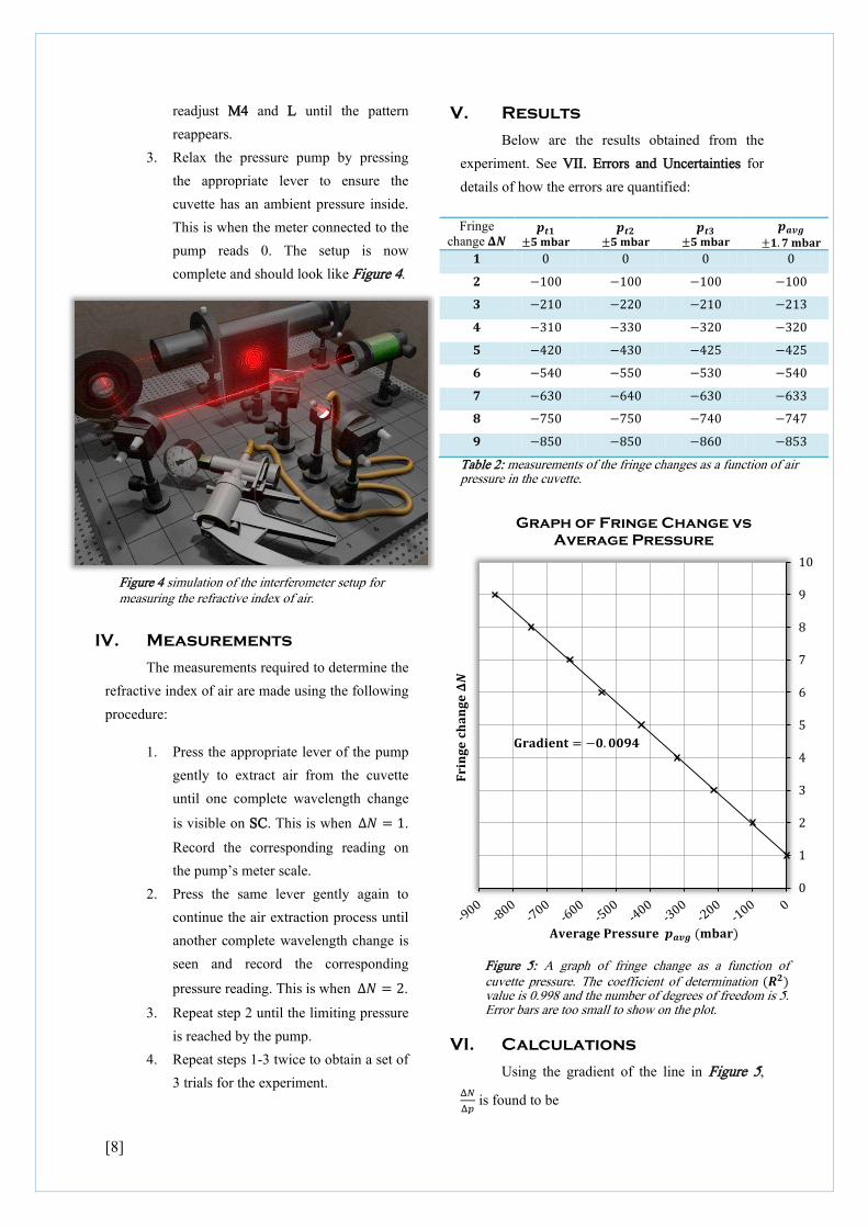
3. Relax the pressure pump by pressing

the appropriate lever to ensure the

cuvette has an ambient pressure inside.

This is when the meter connected to the

pump reads 0. The setup is now

complete and should look like Figure 4.

IV. Measurements

The measurements required to determine the

refractive index of air are made using the following

procedure:

1. Press the appropriate lever of the pump

gently to extract air from the cuvette

until one complete wavelength change

is visible on SC. This is when Δ𝑁 = 1.

Record the corresponding reading on

the pump’s meter scale.

2. Press the same lever gently again to

continue the air extraction process until

another complete wavelength change is

seen and record the corresponding

pressure reading. This is when Δ𝑁 = 2.

3. Repeat step 2 until the limiting pressure

is reached by the pump.

4. Repeat steps 1-3 twice to obtain a set of

3 trials for the experiment.

V. Results

Below are the results obtained from the

experiment. See VII. Errors and Uncertainties for

details of how the errors are quantified:

Fringe change 𝚫𝑵

𝒑𝒕𝟏 ±𝟓 𝐦𝐦𝐆𝐆

𝒑𝒕𝟐 ±𝟓 𝐦𝐦𝐆𝐆

𝒑𝒕𝟑 ±𝟓 𝐦𝐦𝐆𝐆

𝒑𝒂𝒂𝒂 ±𝟏.𝟕 𝐦𝐦𝐆𝐆

𝟏 0 0 0 0

𝟐 −100 −100 −100 −100

𝟑 −210 −220 −210 −213

𝟎 −310 −330 −320 −320

𝟓 −420 −430 −425 −425

𝟔 −540 −550 −530 −540

𝟕 −630 −640 −630 −633

𝟖 −750 −750 −740 −747

𝟎 −850 −850 −860 −853

Table 2: measurements of the fringe changes as a function of air pressure in the cuvette.

VI. Calculations

Using the gradient of the line in Figure 5,

Δ𝑁Δ𝑝

is found to be

0

1

2

3

4

5

6

7

8

9

10

Graph of Fringe Change vs Average Pressure

Figure 4 simulation of the interferometer setup for measuring the refractive index of air.

Figure 5: A graph of fringe change as a function of cuvette pressure. The coefficient of determination (𝑹𝟐) value is 0.998 and the number of degrees of freedom is 5. Error bars are too small to show on the plot.

𝐆𝐆𝐆𝐆𝐆𝐆𝐆𝐆 = −𝟎.𝟎𝟎𝟎𝟎

𝐀𝐀𝐆𝐆𝐆𝐀𝐆 𝐏𝐆𝐆𝐏𝐏𝐏𝐆𝐆 𝒑𝒂𝒂𝒂 (𝐦𝐦𝐆𝐆)

𝐅𝐆𝐆𝐆𝐀𝐆

𝐜𝐜𝐆𝐆𝐀𝐆 𝚫𝑵

[9]

Also, using the depth of the cuvette 𝑠 = 10 mm

and the wavelength of the laser 𝜆 = 632.8 nm, the

change of refractive index with pressure, Δ𝑛Δ𝑝

may be

found by substituting these values, together with

(8), into (7):

Δ𝑛Δ𝑝

= −Δ𝑁Δ𝑝

𝜆2𝑠

= 0.0094632.8 × 10−9

2 × 10 × 10−3

Δ𝑛Δ𝑝

= (2.928 ± 0.125) × 10−7 mbar−1.

Finally, substituting this into (4) yields:

𝑛(𝑝) = 1 +Δ𝑛Δ𝑝

𝑝0 = 1 + (2.928 × 10−7) × 1013

∴ 𝒏𝒂𝒊𝒓 = 𝟏.𝟎𝟎𝟎𝟐𝟎𝟔 ± 𝟎.𝟎𝟎𝟎𝟎𝟏𝟐.

VII. Errors and Uncertainties

Quantifying errors

The measurement errors in this part of the

experiment are on the readings of pressure, as

displayed on the meter attached to the air extraction

pump (see Figure 4). Based on the scale of this

meter, the eye’s maximum resolvable division

corresponds to a pressure difference of ±5 mbar.

This is then the error quoted on each measurement

in all 3 trials.

Uncertainties

A small uncertainty is present when reading

the values of pressure corresponding to the fringe

changes. As the air extraction lever is released

(once one whole wavelength change is observed),

there is still a flux of air pressure traveling in the

reverse direction – that is; back into the cuvette.

Due to this, the needle of the pressure pump’s

meter does not stay in the position at which the

wavelength change occurs; but drops quite steadily

in the direction of the 0 mark. The effect of this

uncertainty is reduced by pressing the air extraction

lever a slight bit more than necessary and allowing

the needle to drop to the position where the

wavelength changes by a whole, as visible on SC.

The pressure is read off at this point.

As in Part 2, an additional uncertainty, in

spotting when exactly the fringe changes by one

whole wavelength, is also present here. The effect

of this is reduced in the same way.

VIII. References - Queen Mary, Department of Physics. Laboratory

Manual – Experiment 5: Building a Michelson

Interferometer, pages 6-7.

- Eugene Hecht (2002). Optics, ed.4, pages 66-70.

Conclusion I. Analysis of Results

Part 2: Measuring magnetostriction

In Part 2, a graph of the magnetostriction of

iron and nickel was plotted using the data collected

experimentally. The graph, together with that given

in literature, is shown in Figure 6.

Δ𝑁Δ𝑝

= −0.0094 ±0.0004 mbar−1. (8)

Graph of Magnetostriction of Iron and Nickel

𝐌𝐆𝐀𝐆𝐆𝐆𝐆𝐜 𝐟𝐆𝐆𝐟𝐆 𝐏𝐆𝐆𝐆𝐆𝐀𝐆𝐜 𝟏𝟎𝟑𝐀𝐦−𝟏

𝐑𝐆𝐟𝐆𝐆𝐆𝐀𝐆 𝐟𝐆𝐆𝐀𝐆𝐜

𝐜𝐜𝐆𝐆𝐀𝐆 𝟏𝟎

−𝟔

Figure 6: a combined graph of the magnetostriction of iron and nickel, plotted in Part 2 of this experiment, with that given in literature.

Iron (experiment)

Iron (literature)

Nickel (experiment)

Nickel (literature)

[10]

According to the convention established in

Part 2 – that the sourcing fringes are positive and

the sinking ones negative – and the fact that the

distance M2 – BS, in the interferometer setup, is

less than the distance BS – M3: a sourcing fringe

pattern on SC corresponds to the lengthening of the

metal sample whereas a sinking pattern indicates its

contraction. Considering this, we can use Figure 6

to understand the behaviour of both samples when

under the effect of an applied magnetic field –

namely that, as the field magnitude increases:

• iron initially extends steadily in length and

then contracts below its equilibrium length

in a damped-exponential fashion, and

• nickel contracts only, in an undamped-

exponential manner.

Additionally, if one compares, using Figure

6, the experimentally plotted graph with the one

given in literature, it is clear that:

• it follows the general trend very closely, and

• the iron sample extends more, slower, and it

also shortens more, but faster, and

• the nickel sample shortens at about the same

rate, but it does not reach that extent of

shortening.

The range of data is also less, but this is due

to the maximum current limit that could be

supplied to the coil. More readings would help

define the shape of the iron sample’s graph better.

Part 3: Measuring refractive index of air

In Part 3, an adapted version of the

interferometer is used to determine the refractive

index of air. This was calculated to be:

𝑛𝑒𝑥𝑝𝑎𝑖𝑟 = 1.000296 ± 0.000012

and the literary value, at normal temperature and

pressure, is

𝑛𝑙𝑖𝑡𝑎𝑖𝑟 = 1.000269

Upon comparison of these two figures, it is

clear that the experimentally determined value is

very close to the literary one as it is accurate to the

fourth decimal place. This accuracy is due to the

quality of the best line fit in Figure 5, which shows

that the experimentally obtained data is strongly in

agreement with the linear relationship between the

changes in refractive index and pressure of a gas.

II. Summary

This experiment begun with the construction

of a Michelson interferometer. Using it, the

behaviour, of two ferromagnetic samples (iron and

nickel) when under the application of an external

magnetic field, was observed. It was found that iron

initially expands and then contracts while nickel

contracts only.

Lastly, the setup of the interferometer was

modified, with the placement of a cuvette

connected to an air extraction pump in one of the

beam paths, in order to allow the measurement of

refractive index changes with pressure inside the

cuvette. Through this, the refractive index of air

was calculated to be

𝑛𝑒𝑥𝑝𝑎𝑖𝑟 = 1.000296 ± 0.000012.