Instructions for use

Title Evolution of the north-polar cap of Mars : a modelling study

Author(s) Greve, Ralf; Mahajan, Rupali A.; Segschneider, Joachim; Grieger, Björn

Citation Planetary and Space Science, 52(9), 775-787https://doi.org/10.1016/j.pss.2004.03.007

Issue Date 2004-08

Doc URL http://hdl.handle.net/2115/32734

Type article (author version)

File Information Greve_etal_2004_PSS.pdf

Hokkaido University Collection of Scholarly and Academic Papers : HUSCAP

Planet. Space Sci. 52 (9), 775–787, 2004http://www.elsevier.com/locate/pss

— Authors’ final version —

Evolution of the north-polar cap of Mars:

a modelling study

Ralf Greve (1,2), Rupali A. Mahajan (3),

Joachim Segschneider (3) and Bjorn Grieger (3)

(1) Institute of Low Temperature Science, Hokkaido University,

Kita-19, Nishi-8, Kita-ku, Sapporo 060-0819, Japan

(2) Department of Mechanics, Darmstadt University of Technology,

Hochschulstraße 1, D-64289 Darmstadt, Germany

(3) Max Planck Institute for Aeronomy,

Max-Planck-Straße 2, D-37191 Katlenburg-Lindau, Germany

March 29, 2004

Correspondence to: R. Greve (greve@lowtem.hokudai.ac.jp)

1

Abstract

Celestial-mechanical computations show that, even stronger than for Earth, Mars is subject

to Milankovic cycles, that is, quasi-periodic variations of the orbital parameters obliquity,

eccentricity and precession. Consequently, solar insolation varies on time-scales of 104–105

years. It has long been supposed that this entails climatic cycles like the terrestrial glacial-

interglacial cycles. This hypothesis is supported by the light-dark layered deposits of the

north- and south-polar caps indicating a strongly varying dust content of the ice due to

varying climate conditions in the past. This study aims at simulating the dynamic and

thermodynamic evolution of the north-polar cap (NPC) of Mars with the ice-sheet model

SICOPOLIS. The boundary conditions of surface accumulation, ablation and temperature

are derived directly from the solar-insolation history by applying the newly developed

Mars Atmosphere-Ice Coupler MAIC. We consider steady-state scenarios under present

climate conditions as well as transient scenarios over climatic cycles. It is found that the

NPC is most likely not in steady state with the present climate. The topography of the

NPC is mainly controlled by the history of the surface mass balance. Ice flow, which is

of the order of 1 mm a−1, plays only a minor role. In order to build up the present cap

during the last five million years of relatively low obliquities, a present accumulation rate

of ≥ 0.25 mm water equiv. a−1 is required. Computed basal temperatures are far below

pressure melting for all simulations and all times.

1 Introduction

The Martian poles are both covered by ice caps. The seasonal caps, which can extend

down to latitudes of approximately 55◦N/S, consist of only some ten centimeters of CO2

snow which sublimes into the atmosphere during the respective spring season. The smaller

residual caps poleward of approximately 80◦N/S are underlain by massive topographic

structures known as the polar layered deposits (Thomas et al. 1992). The complexes

composed of the residual caps and the layered deposits are referred to as the north- and

south-polar cap (NPC/SPC), respectively (e.g., Johnson et al. 2000, Byrne and Murray

2002, Greve et al. 2003). Owing to the Mars Orbiter Laser Altimeter (MOLA) measure-

ments of the Mars Global Surveyor (MGS) spacecraft, the surface topographies of the NPC

and SPC have been mapped very precisely (Zuber et al. 1998, Smith et al. 1999). The

NPC topography, which is our focus, is shown in Fig. 1 (left panel).

This study is a continuation of previous ones by Greve (2000b) and Greve et al. (2003)

in which the NPC was treated in a simplified fashion as a paraboloid cap. The topography

evolution was prescribed because of limited knowledge about climatic forcing. Here, we

2

Figure 1: Left: MOLA surface topography of the north-polar cap, z = h(x, y, t=0)

(in km relative to the reference geoid; Zuber et al. 1998, Smith et al. 1999). Right:

Computed topography of the equilibrated ground for ice-free conditions, z = b0(x, y)

(in km relative to the reference geoid). The heavy-dashed line in each panel indicates

the ice margin.

30

Figure 1: Left: MOLA surface topography of the north-polar cap, z = h(x, y, t=0) (in kmrelative to the reference geoid; Zuber et al. 1998, Smith et al. 1999). Right: Computedtopography of the equilibrated ground for ice-free conditions, z = b0(x, y) (in km relativeto the reference geoid). The heavy-dashed line in each panel indicates the ice margin.

aim at overcoming this simplification by constructing a simple model called MAIC (Mars

Atmosphere-Ice Coupler). MAIC parameterizes the surface temperature, ice accumulation

and ablation mainly as a function of the Milankovic parameter obliquity (e.g., Laskar et al.

2002). Dynamic/thermodynamic simulations are carried out for the NPC with the ice-sheet

model SICOPOLIS (SImulation COde for POLythermal Ice Sheets). Two different types

of simulations are considered: (i) steady-state simulations in which the present climate

forcing is assumed to be constant over time, and (ii) transient simulations which model

explicitly the evolution of the NPC over climatic cycles. Hereby, our central presumption

is that the NPC consists mainly of H2O ice with physical properties comparable to that

of ice in terrestrial ice sheets, so that the NPC is controlled by accumulation, ablation

and glacial flow (which are, of course, orders of magnitude smaller than on Earth). Greve

et al. (2003) discussed the validity of this presumption in some detail, therefore this is not

repeated here.

2 Ice-sheet model SICOPOLIS

The dynamic/thermodynamic behaviour of the NPC of Mars is investigated with the

ice-sheet model SICOPOLIS. It was originally developed for terrestrial ice sheets and

successfully applied to problems of past, present and future glaciation of Greenland, the

entire northern hemisphere and Antarctica (cf. Greve 2000a, and references therein). The

model describes ice rheologically as an incompressible, heat-conducting, power-law fluid

3

with thermo-mechanical coupling due to the strong temperature dependence of the ice

viscosity. The strain-rate tensor D = sym grad v (velocity v) is given as

D = EA(T ′)σn−1 tD, (1)

where tD the Cauchy stress deviator, σ = [tr (tD)2/2]1/2 the effective shear stress, n the

power-law exponent,

A(T ′) = A0 e−Q/RT ′(2)

the flow-rate factor in the form of an Arrhenius law (A0: preexponential constant, Q:

activation energy, R: universal gas constant, T ′: temperature relative to the pressure

melting point; see Paterson 1994), and E the flow-enhancement factor. The latter is equal

to unity for pure ice and can deviate from unity due to the softening or stiffening effect

of impurities in the ice. It is distinguished between cold ice with a temperature below

the pressure melting point and temperate ice with a temperature at the pressure melting

point. The latter is considered as a binary mixture of ice and small amounts of water. The

interface that separates cold and temperate ice is monitored using Stefan-type energy flux

and mass flux matching conditions.

The model computes the temporal evolution of ice extent, thickness, three-dimensional

velocity, temperature, water content and age in response to external forcing. The latter

is specified by (i) the mean annual air temperature at the ice surface, (ii) the surface

mass balance, that is ice accumulation (snowfall, condensation) minus ablation (melting,

sublimation, erosion), (iii) the global sea level (not relevant for Martian applications in

the recent past) and (iv) the geothermal heat flux heating the ice mass from below. All

computations are carried out in a stereographic plane with standard parallel 71◦N, spanned

by the Cartesian coordinates x and y. The vertical coordinate z is taken positive upward,

and the zero level is the reference geoid. The distortions due to the stereographic projection

are corrected by appropriate metric coefficients.

Isostatic depression and rebound of the lithosphere due to changing ice load is described

by a local-lithosphere-relaxing-asthenosphere (LLRA) model with an isostatic time lag τiso

(Le Meur and Huybrechts 1996, Greve 2001). Owing to the non-local response of the elastic

lithosphere plate, local isostatic compensation of the ice load is not likely. We consider this

by introducing a fraction of isostatic compensation, fiso, so that the steady-state downward

displacement of the lithosphere, wss, is

wss = fiso ×Hρ

ρa

, (3)

where H is the ice thickness, ρ the ice density and ρa the asthenosphere (upper-mantle)

4

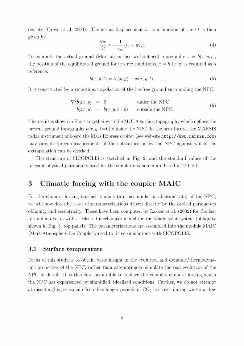
density (Greve et al. 2003). The actual displacement w as a function of time t is then

given by∂w

∂t= − 1

τiso

(w − wss). (4)

To compute the actual ground (Martian surface without ice) topography z = b(x, y, t),

the position of the equilibrated ground for ice-free conditions, z = b0(x, y) is required as a

reference:

b(x, y, t) = b0(x, y)− w(x, y, t). (5)

It is constructed by a smooth extrapolation of the ice-free ground surrounding the NPC,

∇2b0(x, y) = 0 under the NPC,

b0(x, y) = b(x, y, t=0) outside the NPC.(6)

The result is shown in Fig. 1 together with the MOLA surface topography which defines the

present ground topography b(x, y, t=0) outside the NPC. In the near future, the MARSIS

radar instrument onboard the Mars Express orbiter (see website http://www.marsis.com)

may provide direct measurements of the subsurface below the NPC against which this

extrapolation can be checked.

The structure of SICOPOLIS is sketched in Fig. 2, and the standard values of the

relevant physical parameters used for the simulations herein are listed in Table 1.

3 Climatic forcing with the coupler MAIC

For the climatic forcing (surface temperature, accumulation-ablation rate) of the NPC,

we will now describe a set of parameterizations driven directly by the orbital parameters

obliquity and eccentricity. These have been computed by Laskar et al. (2002) for the last

ten million years with a celestial-mechanical model for the whole solar system (obliquity

shown in Fig. 3, top panel). The parameterizations are assembled into the module MAIC

(Mars Atmosphere-Ice Coupler), used to drive simulations with SICOPOLIS.

3.1 Surface temperature

Focus of this study is to obtain basic insight in the evolution and dynamic/thermodyna-

mic properties of the NPC, rather than attempting to simulate the real evolution of the

NPC in detail. It is therefore favourable to replace the complex climatic forcing which

the NPC has experienced by simplified, idealized conditions. Further, we do not attempt

at disentangling seasonal effects like longer periods of CO2 ice cover during winter at low

5

Figure 2: Sketch of the ice-sheet model SICOPOLIS with the coupler MAIC. Rect-

angular boxes correspond to prognostic model components, oval boxes to inputs from

outside the system.

31

Figure 2: Sketch of the ice-sheet model SICOPOLIS with the coupler MAIC. Rectangularboxes correspond to prognostic model components, oval boxes to inputs from outside thesystem.

obliquity, or seasonal insolation variations due to eccentricity, and formulate the entire

parametrization in mean annual quantities only.

We approximate the obliquity θ for the last four million years, during which the average

was close to the present value θ0 = 25.2◦, by a simplified two-cycle obliquity. To this end,

we define the main cycle

θ(t) = θ0 + θ(t) sin2πt

tmainobl

(7)

with the period tmainobl = 125 ka. The modulation of the amplitude (envelope) is given by

θ(t) =θmax + θmin

2−(

θmax − θmin

2

)cos

2πt

tmodobl

, (8)

with the maximum amplitude θmax = 10◦, the minimum amplitude θmin = 2.5◦ and the

period tmodobl = 1.3 Ma (cf. Ward 1992, Touma and Wisdom 1993, Laskar et al. 2002). The

resultant obliquity history is shown in Fig. 3 (bottom panel, left ordinate axis).

The mean annual insolation at the north pole of Mars, I innp(t), follows from the obliquity

6

Quantity Value

Gravity acceleration, g 3.72 m s−2

Density of ice, ρ 910 kg m−3

Power-law exponent, n 3Flow-enhancement factor, E 3Preexponential constant, A0 3.985× 10−13 s−1 Pa−3

Activation energy, Q 60 kJ mol−1

Universal gas constant, R 8.314 J mol−1 K−1

Heat conductivity of ice, κ 9.828 e−0.0057 T [K] W m−1K−1

Specific heat of ice, c (146.3 + 7.253 T [K]) J kg−1K−1

Latent heat of ice, L 335 kJ kg−1

Clausius-Clapeyron gradient, β 3.3× 10−4 K m−1

Geothermal heat flux, qgeo 35 mW m−2

Fraction of isostaticcompensation, fiso 0.65Isostatic time lag, τiso 3000 aAsthenosphere density, ρa 3300 kg m−3

Density × specific heat of thelithosphere, ρrcr 2000 kJ m−3K−1

Heat conductivity of thelithosphere, κr 3 W m−1K−1

Table 1: Standard physical parameters of the ice-sheet model.

θ and the eccentricity e as

I innp =

Is

πsin θ (1− e2)−1/2 (9)

(Kieffer and Zent 1992), where Is = 590 W m−2 is the solar flux at the average Martian

distance from the sun. Since for the last ten million years, the eccentricity has been limited

by 0 < e < 0.12 (Laskar et al. 2002), it is clear that the influence of the obliquity in Eq. (9)

outweighs by far that of the eccentricity, so that we set e = 0 for simplicity.

Assuming near-steady-state conditions, I innp is in balance with the outgoing mean annual

longwave radiation, Ioutnp ,

I innp (1− A) = Iout

np , (10)

where A is the albedo. According to the Stefan-Boltzmann law, the outgoing radiation is

Ioutnp = εσT 4

np, (11)

where σ = 5.67 × 10−8 W m−2 K−4 is the Stefan-Boltzmann constant, ε is the emissivity

and Tnp is the mean annual surface temperature at the north pole. Inserting (11) in (10)

7

Figure 3: Top: Obliquity θ by Laskar et al. (2002) for the last ten million years. Bot-

tom: Simplified two-cycle obliquity (left ordinate) and resulting mean-annual surface

temperature at the north pole Tnp (right ordinate) for the last four million years.

32

Figure 3: Top: Obliquity θ by Laskar et al. (2002) for the last ten million years. Bottom:Simplified two-cycle obliquity (left ordinate) and resulting mean-annual surface tempera-ture at the north pole Tnp (right ordinate) for the last four million years.

and solving for Tnp yields

Tnp(t) =(I in

np(t) (1− A)

εσ

)1/4

. (12)

With albedo A = 0.43 (Thomas et al. 1992), the emissivity ε taken as unity and the present

insolation I innp(0) = 79.96 W m−2, we obtain the present temperature Tnp(0) = 168.4 K. The

temperature history, which varies by ca. 30K within the considered range of obliquities, is

depicted in Fig. 3 (bottom panel, right ordinate axis).

The above albedo and emissivity values are interpreted as long-term averages for the

NPC, therefore temporal changes are not accounted for. If we assume an uncertainty of

∆A = 0.05 for the albedo and of ∆ε = 0.1 for the emissivity, the terms (1 − A) and 1/ε

in Eq. (12) are both afflicted with relative errors of approx. 10%. According to the rules

of error propagation, either of these yield a relative error of 2.5% for Tnp. In absolute

terms, this is approx. ±4 K due to the albedo uncertainty and +4 K due to the emissivity

uncertainty (ε > 1 is of course physically meaningless).

The mean annual surface temperature for an arbitrary position x, y on the polar cap,

8

Ts, is now prescribed similarly to Greve (2000b) and Greve et al. (2003),

Ts(x, y, t) = Tnp(t) + cs φ(x, y), (13)

where φ is the co-latitude and cs the co-latitude coefficient. In contrast to the earlier

studies, we have refrained here from introducing an explicit dependency on elevation by an

atmospheric temperature lapse rate. The reason is that the computation of the north-polar

surface temperature according to Eq. (12) is based on the idea of a radiation-dominated

environment due to the tenuous Martian atmosphere. Because of this, it is consequent

to attribute the surface warming off the north pole to the increasing insolation with in-

creasing distance from the north pole (co-latitude), and not to the decreasing surface

elevation. Therefore, the warming is parameterized by the co-latitude coefficient only, and

as a suitable value cs = 2.25 K (◦co-lat)−1 is chosen. Note that the surface-temperature

parametrization described by Eqs. (12) and (13) is not influenced directly by atmospheric

pressure variations.

3.2 Accumulation-ablation rate

The accumulation rate a+sat (“saturation accumulation”) over the north-polar cap is as-

sumed to be proportional to the water-vapour saturation pressure in the atmosphere psat,

which is given by the Clausius-Clapeyron relation (e.g. Muller 2001),

a+sat(t) ∝ psat(t) ∝ exp

(− λ

RmTref(t)

), (14)

with the latent heat λ = λsol→liq + λliq→vap = (335 + 2525) kJ kg−1 = 2860 kJ kg−1 and the

gas constant Rm = R/MH2O = 8.314 J mol−1 K−1/18.015 kg kmol−1 = 461.5 J kg−1 K−1.

The atmospheric reference temperature for the north-polar region Tref is prescribed as

Tref(t) = T 0ref + ∆Ts(t), (15)

with the present value T 0ref = 173 K and the surface-temperature offset

∆Ts(t) = Tnp(t)− Tnp(0). (16)

With the present accumulation rate a+sat,0, Eqs. (14) and (15) yield

a+sat(t) = a+

sat,0 exp

(λ

RmT 0ref

− λ

RmTref(t)

), (17)

9

which is depicted in Fig. 4. Based on different methods [amount of water vapour in the

atmosphere, shortage of craters, mass-balance modelling; see discussion and references

in Greve (2000b)], a+sat,0 has been estimated to be of the order of 0.1 mm w.e. a−1 – w.e.

denoting water equivalent –, with an uncertainty of a factor ten in either direction. Further,

it is not clear whether H2O-ice accumulation takes place mainly as snowfall, or mainly as

direct condensation at the surface. However, the form of accumulation is of no importance

for our simulations.

Figure 4: Accumulation rate a+sat as a function of surface-temperature offset ∆Ts, for

present value a+sat,0 = 0.1 mm w.e. a−1.

33

Figure 4: Accumulation rate a+sat as a function of surface-temperature offset ∆Ts, for

present value a+sat,0 = 0.1 mm w.e. a−1.

For the net mass balance, that is, the accumulation-ablation rate anet = a+sat − a− (a−:

ablation rate), we propose an equilibrium-line concept dependent on the horizontal distance

from the north pole, d. This is a widely-used approach for terrestrial ice-sheet and glacier

problems, and we employ it in the variant of the ice-sheet-modelling intercomparison study

by Payne et al. (2000). It is given by

anet(x, y, t) = min[a+

sat(t), g(t)× (del(t)− d(x, y))], (18)

where g is the accumulation-ablation-rate gradient and del the distance of the equilibrium

line from the north pole (Fig. 5).

For present conditions, the values of the two parameters d0el and g0 should be chosen

such that the equilibrium line is close to the ice margin. The interior of the north-polar

cap must lie in the accumulation area where anet = a+sat,0. This can be achieved by choosing

d0el = 550 km and g0 = 2.5 × 10−4 mm w.e. a−1 km−1. Thus, for a+

sat,0 = 0.1 mm w.e. a−1

the accumulation area where anet = a+sat,0 lies within d ≤ 150 km, and the distance from

the accumulation area to the equilibrium line is l0g = 400 km (Fig. 5). For other times, we

10

Figure 5: Distance-dependent parametrization of the net mass balance (accumulation-

ablation rate).

34

Figure 5: Distance-dependent parametrization of the net mass balance (accumulation-ablation rate).

assume for simplicity and lack of better knowledge that del is unchanged, so that

del(t) = d0el. (19)

The gradient g is taken proportional to the accumulation rate,

g(t) = g0 ×a+

sat(t)

a+sat,0

, (20)

so that the size of the accumulation area remains constant, and therefore lg(t) = l0g =

400 km.

4 Simulation set-up

The model domain consists of a 1800 km×1800 km square in polar stereographic projection,

centered at the pole (Fig. 1). The horizontal resolution is 20 km, the vertical resolution 21

grid points in the cold-ice column, 11 grid points in the temperate-ice column (if existing)

and 11 grid points in the lithosphere column.

The ice mechanics is described by Eq. (1) with standard values for the terrestrial

Greenland ice sheet, n = 3 and E = 3. This includes the influence of small amounts of fine

dust, ca. 1 mg kg−1 with particle sizes of 0.1 to 2 µm as it was measured in the Wisconsin-

ice-age part of the ice core Dye 3 in south Greenland (Hammer et al. 1985). This makes the

ice more readily deformable than ideally pure ice with E = 1 (Paterson 1991). However,

if major parts of the ice volume were contaminated significantly with dust, the mixture of

11

deformable ice and essentially rigid dust would be even stiffer than pure ice. On the other

hand, the decreased heat conductivity and the increased density of an ice-dust mixture

result in increased basal temperatures and driving stresses, respectively, which both favour

ice flow. The combined effect was discussed by Greve et al. (2003), who concluded that

dust volume fractions of ϕ ≤ 20% alter flow velocities by a factor at maximum of two

and basal temperatures by less than 5◦C. For larger dust contents the deviations would

increase rapidly.

Initial conditions are defined by an ice-free state with isostatically equilibrated ground.

Owing to the large average obliquities between ten and five million years ago, it is likely

that this was the real situation during this period (Laskar et al. 2002; Forget, pers. comm.

2003; see also Fig. 3). A formation of the present NPC during the last millions of years

is also consistent with the results by Herkenhoff and Plaut (2000). Based on the observed

absence of craters larger than 300 m at the surface of the NPC, they estimate a surface

age of approx. 100 ka and a resurfacing rate of approx. 1 km per Ma.

At the ice-bedrock interface, no-slip conditions are applied regardless of the basal tem-

perature. For the geothermal heat flux, the value qgeo = 35 mW m−2 is used as standard

(Budd et al. 1986, Schubert et al. 1992); this is about 2/3 of the average geothermal heat

flux on Earth. The standard value of the fraction of isostatic compensation is chosen

as fiso = 0.65, approximately 2/3 of full local compensation, which was found to be a

likely estimate in the previous study by Greve et al. (2003) where a more sophisticated

viscoelastic multi-layer ground model was applied.

As it was mentioned at the beginning of Sect. 3.1, in this study we aim at investigating

the evolution and dynamic response of the NPC under simplified, idealized conditions,

rather than employing the real, complex climatic forcing with a whole spectrum of fre-

quencies. Therefore, two types of simulations are carried out: (i) steady-state simulations

for present climate conditions, and (ii) transient simulations over idealized climate cy-

cles. In the steady-state runs, the obliquity is kept constant over time at its present value

θ0 = 25.2◦. This implies a north-polar surface temperature of Tnp = 168.4 K ≈ − 105◦C,

and ∆Ts(t) ≡ 0 (Sect. 3.1). For the surface-temperature parametrization (13), we use

the co-latitude coefficient cs = 2.25 K (◦co-lat)−1. Standard settings for the parame-

ters in the accumulation-ablation model are a+sat = 0.1 mm w.e. a−1, del = 550 km and

g = 2.5 × 10−4 mm w.e. a−1 km−1. In order to assess the influence of the several parame-

ters on the dynamics of the NPC, additional simulations are run with varied parameters;

see Table 2. All steady-state simulations are integrated with a time-step of 10 ka for

500 Ma until the dynamic and thermodynamic equilibrium.

For the transient runs, we use the simplified two-cycle obliquity forcing of Sect. 3.1. Like

for the steady-state simulations, the standard run has the surface-temperature parameter

12

Run Parameter variations#1 None (standard set)#2 a+

sat = 1 mm w.e. a−1, g = 2.5× 10−3 mm w.e. a−1 km−1

#3 a+sat = 0.01 mm w.e. a−1, g = 2.5× 10−5 mm w.e. a−1 km−1

#4 qgeo = 20 mW m−2

#5 qgeo = 50 mW m−2

#6 E = 0.3#7 E = 30#8 fiso = 0#9 fiso = 1

Table 2: Set-up for the steady-state simulations.

cs = 2.25 K (◦co-lat)−1, and the accumulation-ablation parameters a+sat,0 = 0.1 mm w.e. a−1,

d0el = 550 km, g0 = 2.5 × 10−4 mm w.e. a−1 km−1. The transient standard run starts from

ice-free conditions as the steady-state simulations. An additional run is conducted that

uses the present MOLA topography as initial condition. Both simulations are integrated

with a time-step of 5 ka over 100 Ma.

5 Results and discussion

5.1 Steady-state runs

The evolution of the total ice volume, Vtot, and the ice-covered area, A, are shown in

Fig. 6 for the standard steady-state run. Over the first 100 Ma, the ice volume increases

essentially linearly. The steady-state value, 5.62× 106 km3, is reached after 250 Ma. The

ice-covered area shows a slightly different behaviour. Over the first 50 Ma, it remains

essentially constant at 1.00 × 106 km2, the size of the area with a positive surface mass

balance (accumulation-ablation rate). Then, the area starts to increase, because due to

increasing ice flow the ice cap spreads into the ablation zone. Finally, at ca. 250 Ma, the

steady-state value of 2.19 × 106 km2 is reached. Both the steady-state volume and area

are much larger than the respective values of the present ice cap, which are estimated

as Vtot = 1.2 . . . 1.7 × 106 km3 and Ai,b = 106 km2 from the MOLA topography. Further,

since the real Martian climate will not have been constant over a period as long as 250 Ma

regarding the much shorter obliquity cycles, it is clear that the NPC cannot be expected

to be in a steady state.

Therefore, we define the build-up time for the present cap, tbuild, as the time the NPC

requires to reach the MOLA value for the present maximum surface elevation, hmax =

−1.95 km (with respect to the reference geoid), when starting from ice-free conditions.

13

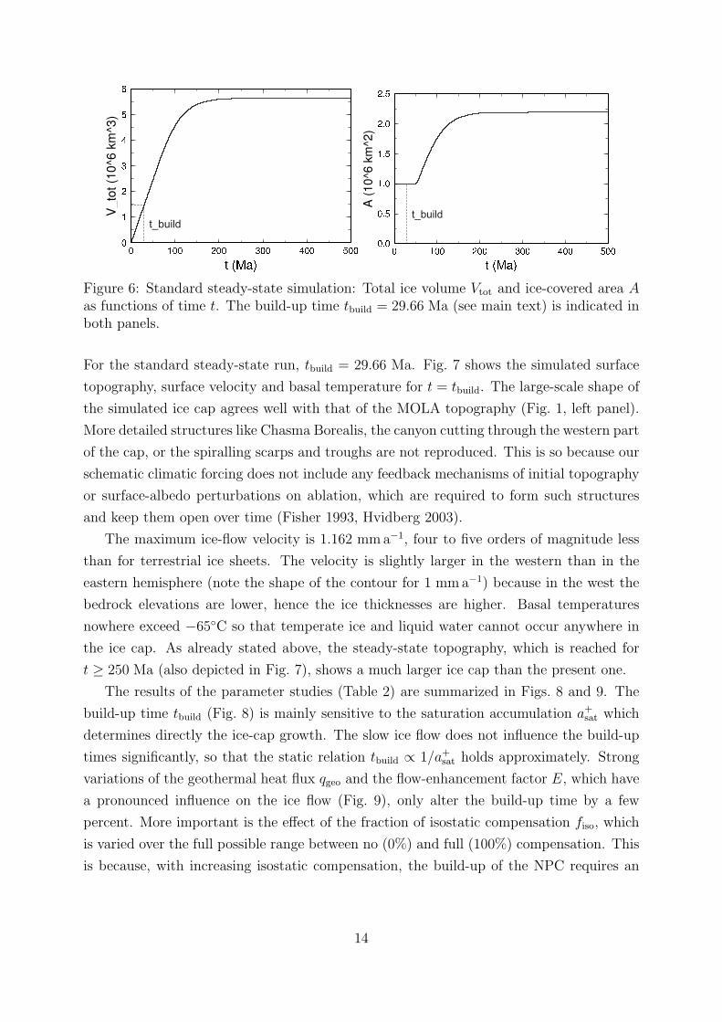
Figure 6: Standard steady-state simulation: Total ice volume Vtot and ice-covered

area A as functions of time t. The build-up time tbuild = 29.66 Ma (see main text) is

indicated in both panels.

35

Figure 6: Standard steady-state simulation: Total ice volume Vtot and ice-covered area Aas functions of time t. The build-up time tbuild = 29.66 Ma (see main text) is indicated inboth panels.

For the standard steady-state run, tbuild = 29.66 Ma. Fig. 7 shows the simulated surface

topography, surface velocity and basal temperature for t = tbuild. The large-scale shape of

the simulated ice cap agrees well with that of the MOLA topography (Fig. 1, left panel).

More detailed structures like Chasma Borealis, the canyon cutting through the western part

of the cap, or the spiralling scarps and troughs are not reproduced. This is so because our

schematic climatic forcing does not include any feedback mechanisms of initial topography

or surface-albedo perturbations on ablation, which are required to form such structures

and keep them open over time (Fisher 1993, Hvidberg 2003).

The maximum ice-flow velocity is 1.162 mm a−1, four to five orders of magnitude less

than for terrestrial ice sheets. The velocity is slightly larger in the western than in the

eastern hemisphere (note the shape of the contour for 1 mm a−1) because in the west the

bedrock elevations are lower, hence the ice thicknesses are higher. Basal temperatures

nowhere exceed −65◦C so that temperate ice and liquid water cannot occur anywhere in

the ice cap. As already stated above, the steady-state topography, which is reached for

t ≥ 250 Ma (also depicted in Fig. 7), shows a much larger ice cap than the present one.

The results of the parameter studies (Table 2) are summarized in Figs. 8 and 9. The

build-up time tbuild (Fig. 8) is mainly sensitive to the saturation accumulation a+sat which

determines directly the ice-cap growth. The slow ice flow does not influence the build-up

times significantly, so that the static relation tbuild ∝ 1/a+sat holds approximately. Strong

variations of the geothermal heat flux qgeo and the flow-enhancement factor E, which have

a pronounced influence on the ice flow (Fig. 9), only alter the build-up time by a few

percent. More important is the effect of the fraction of isostatic compensation fiso, which

is varied over the full possible range between no (0%) and full (100%) compensation. This

is because, with increasing isostatic compensation, the build-up of the NPC requires an

14

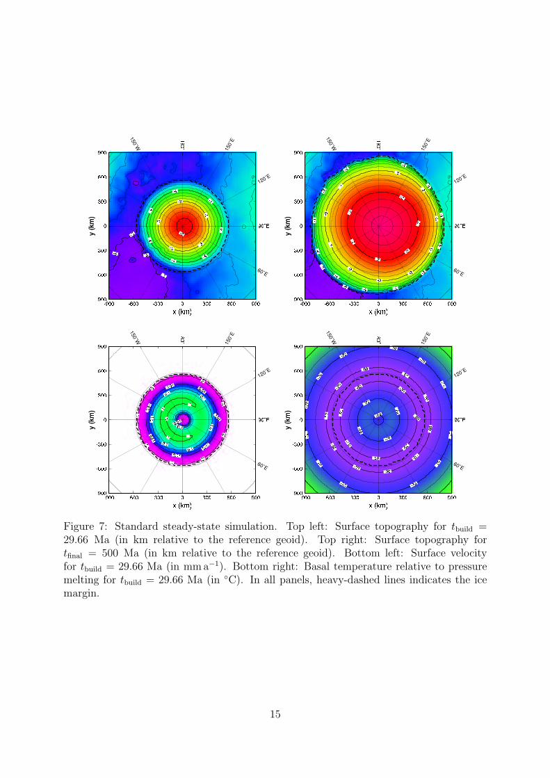
Figure 7: Standard steady-state simulation. Top left: Surface topography for tbuild =

29.66 Ma (in km relative to the reference geoid). Top right: Surface topography

for tfinal = 500 Ma (in km relative to the reference geoid). Bottom left: Surface

velocity for tbuild = 29.66 Ma (in mma−1). Bottom right: Basal temperature relative

to pressure melting for tbuild = 29.66 Ma (in ◦C). In all panels, heavy-dashed lines

indicates the ice margin.

36

Figure 7: Standard steady-state simulation. Top left: Surface topography for tbuild =29.66 Ma (in km relative to the reference geoid). Top right: Surface topography fortfinal = 500 Ma (in km relative to the reference geoid). Bottom left: Surface velocityfor tbuild = 29.66 Ma (in mm a−1). Bottom right: Basal temperature relative to pressuremelting for tbuild = 29.66 Ma (in ◦C). In all panels, heavy-dashed lines indicates the icemargin.

15

2.9529.66

310.9

0.01 0.1 1

t_bu

ild (

Ma)

a_sat^+ (mm w.e./a)

29.529.66

30.11

20 35 50

t_bu

ild (

Ma)

q_geo (mW/m2)

29.529.66

30.96

0.3 3 30

t_bu

ild (

Ma)

E (1)

24.53

29.66

33.45

0 0.65 1

t_bu

ild (

Ma)

f_iso (1)

Figure 8: Steady-state simulations: Build-up time tbuild as a function of the saturation

accumulation a+sat, the geothermal heat flux qgeo, the flow-enhancement factor E and

the fraction of isostatic compensation fiso.

37

Figure 8: Steady-state simulations: Build-up time tbuild as a function of the saturationaccumulation a+

sat, the geothermal heat flux qgeo, the flow-enhancement factor E and thefraction of isostatic compensation fiso.

0.49

1.162

1.939

0.01 0.1 1

vs_m

ax (

mm

/a)

a_sat^+ (mm w.e./a)

0.316

1.162

2.96

20 35 50

vs_m

ax (

mm

/a)

q_geo (mW/m2)

0.269

1.162

4.705

0.3 3 30

vs_m

ax (

mm

/a)

E (1)

0.47

1.162

1.872

0 0.65 1

vs_m

ax (

mm

/a)

f_iso (1)

Figure 9: Steady-state simulations: Maximum surface velocity vs,max as a function of

the saturation accumulation a+sat, the geothermal heat flux qgeo, the flow-enhancement

factor E and the fraction of isostatic compensation fiso.

38

Figure 9: Steady-state simulations: Maximum surface velocity vs,max as a function of thesaturation accumulation a+

sat, the geothermal heat flux qgeo, the flow-enhancement factorE and the fraction of isostatic compensation fiso.

increasing ice thickness. In contrast to the build-up times, the maximum surface velocities

vs,max (Fig. 9) react sensitively to variations of all the investigated parameters. However,

in all cases they fall in the interval between 0.25 mm a−1 and 5 mm a−1, which is still small

16

in absolute terms.

The effect of the uncertainty in surface albedo and emissivity can be estimated as fol-

lows. With the values given in Sect. 3.1, it was found that these uncertainties lead to

surface-temperature uncertainties of approx. 4 K. Since the time-scale for heat conduc-

tion is much shorter than the determined build-up times, this error propagates essentially

undamped down into the ice cap. An ice-temperature uncertainty of 4 K entails an uncer-

tainty of the rate factor (2) of about a factor two, and consequently ice-flow velocities are

affected by a factor two as well. This is comparable to the effect of the varied geothermal

heat flux (Fig. 9), which also changes the ice temperature and therefore speeds up or slows

down the ice flow.

5.2 Transient runs

Similar to Fig. 6 for the standard steady-state run, the evolution of the total ice volume,

Vtot, and the ice-covered area, A, are shown in Fig. 10 for the standard transient run. It

is striking that both curves resemble very much those of the steady-state run, variations

due to the obliquity cycles are barely recognizable. Therefore, the evolution of Vtot and A

is mainly governed by the long-term average climate. This contradicts the approach made

in the previous studies by Greve (2000b) and Greve et al. (2003) where it was assumed

that the climate cycles cause major variations of the ice-cap topography.

Figure 10: Two-cycle-obliquity simulation starting from ice-free conditions: Total

ice volume Vtot and ice-covered area A as functions of time t. The build-up time

tbuild = 13.78 Ma (see main text) is indicated in both panels.

39

Figure 10: Two-cycle-obliquity simulation starting from ice-free conditions: Total ice vol-ume Vtot and ice-covered area A as functions of time t. The build-up time tbuild = 13.78 Ma(see main text) is indicated in both panels.

The build-up time for the present cap is tbuild = 13.78 Ma, as compared to 29.66 Ma

for the standard steady-state run. This is due to the fact that the average saturation

accumulation is larger than its present value, compare Fig. 4 (note the logarithmic scale).

However, this scenario is still unable to build up the present cap within the last five million

17

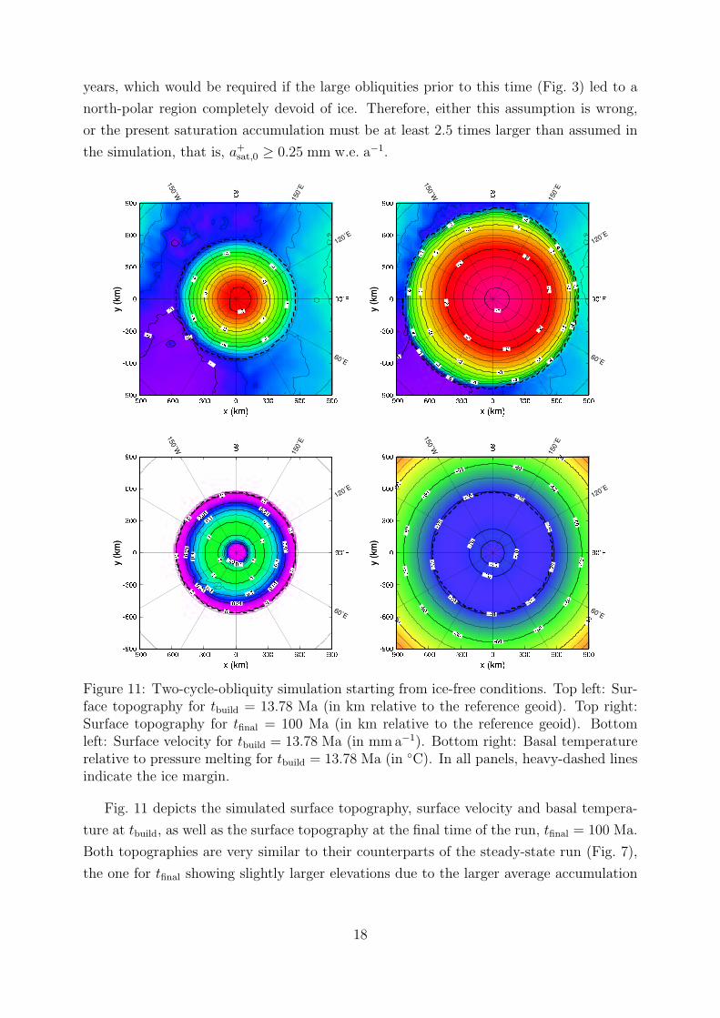
years, which would be required if the large obliquities prior to this time (Fig. 3) led to a

north-polar region completely devoid of ice. Therefore, either this assumption is wrong,

or the present saturation accumulation must be at least 2.5 times larger than assumed in

the simulation, that is, a+sat,0 ≥ 0.25 mm w.e. a−1.

Figure 11: Two-cycle-obliquity simulation starting from ice-free conditions. Top left:

Surface topography for tbuild = 13.78 Ma (in km relative to the reference geoid). Top

right: Surface topography for tfinal = 100 Ma (in km relative to the reference geoid).

Bottom left: Surface velocity for tbuild = 13.78 Ma (in mma−1). Bottom right: Basal

temperature relative to pressure melting for tbuild = 13.78 Ma (in ◦C). In all panels,

heavy-dashed lines indicate the ice margin.

40

Figure 11: Two-cycle-obliquity simulation starting from ice-free conditions. Top left: Sur-face topography for tbuild = 13.78 Ma (in km relative to the reference geoid). Top right:Surface topography for tfinal = 100 Ma (in km relative to the reference geoid). Bottomleft: Surface velocity for tbuild = 13.78 Ma (in mm a−1). Bottom right: Basal temperaturerelative to pressure melting for tbuild = 13.78 Ma (in ◦C). In all panels, heavy-dashed linesindicate the ice margin.

Fig. 11 depicts the simulated surface topography, surface velocity and basal tempera-

ture at tbuild, as well as the surface topography at the final time of the run, tfinal = 100 Ma.

Both topographies are very similar to their counterparts of the steady-state run (Fig. 7),

the one for tfinal showing slightly larger elevations due to the larger average accumulation

18

rate.

The 50% larger flow velocities (vs,max = 1.596 mm a−1) and the up to 10◦C higher basal

temperatures at tbuild (which are still far below pressure melting) are due to the fact that at

this time the surface-temperature deviation is ∆Ts = 12.41◦C, which is by chance close to

the highest temperature throughout the climate cycles. Only 30 ka earlier, at t = 13.75 Ma

when the temperature equals the present one (∆Ts = 0◦C), the maximum surface velocity

is only vs,max = 0.588 mm a−1, thus almost three times smaller.

Figure 12: Two-cycle-obliquity simulation starting from present topography: Surface-

temperature deviation ∆Ts, total ice volume Vtot, ice-covered area A, maximum sur-

face velocity vs,max as functions of time t for the first 1.3 Ma.

41

Figure 12: Two-cycle-obliquity simulation starting from present topography: Surface-temperature deviation ∆Ts, total ice volume Vtot, ice-covered area A, maximum surfacevelocity vs,max as functions of time t for the first 1.3 Ma.

For the transient simulation starting from the MOLA topography, Fig. 12 shows a close-

up of the ice-cap evolution over the first 1.3-Ma cycle only. In these graphs, the influence of

the climatic variations on the ice volume and area can be noted and reveals that the ice cap

is almost stagnant at periods with low surface temperatures, whereas it shows the largest

changes in volume and area at periods with high temperatures. Nevertheless, the absolute

values of these changes are small compared to the longer-term trends. By contrast, the

surface velocity oscillates by a factor of ten, between approximately vs,max = 0.5 mm a−1

and vs,max = 5 mm a−1, maximum velocities following maximum temperatures and vice

19

versa.

Finally, a sequence of surface topographies at intervals of 1 Ma is presented in Fig. 13.

The simulated growth of the ice cap, first in volume, later also in area, is clearly visible.

This is accompanied by a smoothing of small- and medium-scale surface structures under

the influence of the zonally averaged forcing. After 10 Ma, only a small remnant of Chasma

Borealis has survived, and after 20 Ma it has vanished completely. The final state for

100 Ma is essentially the same as that for the standard steady-state run (Fig. 11), implying

that the system has lost the memory of its initial conditions at that time.

Note that the above-determined closure time for Chasma Borealis of ∼ 10 Ma is only a

theoretical value which excludes any feedbacks of the chasm on local meteorological con-

ditions. In reality, it is expected that the chasm creates a major modification of the local

wind circulation pattern by canalizing strong katabatic winds, which affect ice accumu-

lation and ablation processes and lead to enhanced erosion. Further, the lower albedo of

the chasm inevitably leads to higher surface temperatures and increased sublimation rates.

These feedbacks work against the ice flow and may keep the chasm open for an indefinite

period.

Hvidberg (2003) and Hvidberg and Zwally (2003) used a similar ice-flow model and

simulated the topography evolution of the NPC in 2-d (radial distance, elevation) and

high spatial resolution along MOLA tracks, with a focus on the spiralling troughs. They

report that in the absence of any accumulation or ablation, closure times of the troughs

due to ice flow are in the range of 100 ka to 1 Ma. This result fits well to our value for

the much larger Chasma Borealis, which was not considered in their study. They also

report strongly enhanced ice-flow velocities of up to 50 mm a−1 at the steepest scarps,

minimum local sublimation rates of 50 mm a−1 required to keep the troughs open in time

and inward-migration speeds of the troughs of tens of centimeters per year.

Fishbaugh and Head (2002) discussed possible formation mechanisms of Chasma Bore-

alis. Based on an analysis of high-resolution MOLA data and Mars Orbiter Camera (MOC)

and Viking images of the region, they favoured a formation scenario by meltwater outflow

(probably in a jokulhlaup-type event) with subsequent shaping by sublimation and eolian

processes. As possible causes for basal melting, they list the following points: “(1) much

thicker caps, (2) climate change, (3) obliquity change, (4) subcap volcanic eruptions, (5)

the presence of a groundwater mound that reaches the cap base, (6) frictional melting due

to cap movement, (7) higher geothermal heat gradient in the past, (8) inclusion of dust,

salts, clathrates, etc., to modify the melting point, and (9) polar wander.” Point (1) is not

consistent with the results of the standard transient run (our most realistic scenario for

the geologically recent past of the NPC); see Fig. 10. Points (2), (3) and (6) are accounted

for in the simulation and do not raise the basal temperature above −65◦C at any time

20

1 Ma 2 Ma 3 Ma

4 Ma 5 Ma 6 Ma

7 Ma 8 Ma 9 Ma

10 Ma 20 Ma 100 Ma

Figure 13: Two-cycle-obliquity simulation starting from present topography: Surface

topography for t = 1, 2, 3, 4, 5, 6, 7, 8, 9, 10, 20, 100 Ma (in km relative to the

reference geoid). In all panels, heavy-dashed lines indicate the ice margin.

42

Figure 13: Two-cycle-obliquity simulation starting from present topography: Surface to-pography for t = 1, 2, 3, 4, 5, 6, 7, 8, 9, 10, 20, 100 Ma (in km relative to the referencegeoid). In all panels, heavy-dashed lines indicate the ice margin.

21

during the modelled NPC history, so they are inconsistent with our results as well. For

the same reason, point (5) is unlikely. Further, if the NPC was formed in the last millions

of years (geologically the very recent past), significant changes in the average geothermal

heat flow (point 7) and polar wander (point 9) are equally unlikely. Therefore, as possible

causes for meltwater production consistent with our results remain (i) basal warming and

melting-point lowering due to mixed-in dust and salts, and (ii) a temporary heat source

under the ice due to a tectono-thermal event or a volcanic eruption.

6 Summary and outlook

The main findings of this study are:

• The newly developed Mars Atmosphere-Ice Coupler MAIC provides simple parame-

terizations for the climatic input surface temperature and accumulation-ablation rate

required for prognostic simulations of the NPC, driven mainly by the Milankovic pa-

rameter obliquity.

• It is very unlikely that the present NPC is in steady state with the present climate,

because this would require some 100 Ma of essentially unchanged conditions.

• The present large-scale topography of the NPC is mainly controlled by the history

of the surface mass balance. Ice flow, with flow velocities of the order of 1 mm a−1,

plays only a minor role.

• The main obliquity cycles of 125 ka and 1.3 Ma are virtually not reflected in the

evolution of the topography of the NPC, which responds mainly to the long-term

average climate conditions. By contrast, the ice flow shows a strong variation over

the obliquity cycles.

• In order to build up the present cap from ice-free conditions at five million years

before present (which is a possible scenario due to the 25◦ − 45◦ obliquities prior to

this time), a present accumulation rate of ≥ 0.25 mm w.e. a−1 is required.

• In the absence of any counteracting mechanisms like differential ablation or erosion,

the closure time for the canyon Chasma Borealis is of the order of 10 Ma.

• For all simulations and all times, basal temperatures are far below pressure melting.

This result is very robust and was already reported in the previous studies by Greve

(2000b) and Greve et al. (2003).

22

For the future, we plan to run simulations driven directly by the history of Martian

obliquity and eccentricity over the last ten million years by Laskar et al. (2002). The

coupling between the atmosphere and the ice cap will be refined by downscaling simula-

tion results obtained with the atmosphere model PUMA-2 (Portable University Model of

the Atmosphere, Fraedrich et al. 2003; see also http://puma.dkrz.de/puma/) adapted to

Martian conditions (Segschneider et al. 2004, Planet. Space Sci., submitted for publica-

tion). This will further improve the physical basis of the parameterizations for the surface

temperature and the accumulation-ablation rate. Moreover, a study is on the way in order

to investigate in more detail the influence of the ice rheology and the dust content under

the conditions of the NPC (Greve and Mahajan, paper in preparation).

Acknowledgements

The constructive reviews of this paper by J. Eluskiewicz and N. Mangold are gratefully

acknowledged. This work was supported by the Priority Programme 1115 “Mars and the

Terrestrial Planets” of the German Research Foundation (Deutsche Forschungsgemein-

schaft, DFG) under project nos. KE 226/8, GR 1557/4.

References

Budd, W. F., D. Jenssen, J. H. I. Leach, I. N. Smith and U. Radok. 1986. The north polar

ice cap of Mars as a steady-state system. Polarforsch., 56 (1/2), 43–46.

Byrne, S. and B. C. Murray. 2002. North polar stratigraphy and the paleo-erg of Mars. J.

Geophys. Res., 107 (E6), 5044. doi:10.1029/2001JE001615.

Fishbaugh, K. E. and J. W. Head. 2002. Chasma Boreale, Mars: Topographic charac-

terization from Mars Orbiter Laser Altimeter data and implications for mechanisms of

formation. J. Geophys. Res., 107 (E3), 5013. doi:10.1029/2000JE001351.

Fisher, D. A. 1993. If Martian ice caps flow – ablation mechanisms and appearance. Icarus,

105 (2), 501–511.

Fraedrich, K., E. Kirk, U. Luksch and F. Lunkeit. 2003. Ein Zirkulationsmodell fur

Forschung und Lehre. Promet, 29 (1-4), 34–48.

Greve, R. 2000a. Large-scale glaciation on Earth and on Mars. Electronic Publications

Darmstadt No. 816, http://elib.tu-darmstadt.de/diss/000816/. Habilitation thesis, De-

partment of Mechanics, Darmstadt University of Technology, Germany.

23

Greve, R. 2000b. Waxing and waning of the perennial north polar H2O ice cap of Mars

over obliquity cycles. Icarus, 144 (2), 419–431. doi:10.1006/icar.1999.6291.

Greve, R. 2001. Glacial isostasy: Models for the response of the Earth to varying ice loads.

In: B. Straughan, R. Greve, H. Ehrentraut and Y. Wang (Eds.), Continuum Mechanics

and Applications in Geophysics and the Environment, pp. 307–325. Springer, Berlin etc.

Greve, R., V. Klemann and D. Wolf. 2003. Ice flow and isostasy of the north polar cap of

Mars. Planet. Space Sci., 51 (3), 193–204. doi:10.1016/S0032-0633(02)00206-4.

Hammer, C. U., H. B. Clausen, W. Dansgaard, A. Neftel, P. Kristinsdottir and E. Johnson.

1985. Continuous impurity analysis along the Dye 3 deep core. In: C. C. Langway,

H. Oeschger and W. Dansgaard (Eds.), Greenland Ice Core: Geophysics, Geochemistry

and the Environment, Geophysical Monographs No. 33, pp. 90–94. American Geophysical

Union, Washington DC.

Herkenhoff, K. E. and J. J. Plaut. 2000. Surface ages and resurfacing rates of the polar

layered deposits on Mars. Icarus, 144 (2), 243–253.

Hvidberg, C. S. 2003. Relationship between topography and flow in the north polar cap

on Mars. Ann. Glaciol., 37, 363–369.

Hvidberg, C. S. and H. J. Zwally. 2003. Sublimation of water from the north polar cap of

Mars. Abstract, Workshop “Mars Atmosphere Modelling and Observations”, Granada,

Spain, 13–15 Jan. 2003.

Johnson, C. L., S. C. Solomon, J. W. Head, R. J. Phillips, D. E. Smith and M. T. Zuber.

2000. Lithospheric loading by the northern polar cap on Mars. Icarus, 144 (2), 313–328.

Kieffer, H. H. and A. P. Zent. 1992. Quasi-periodic climate change on Mars. In: H. H.

Kieffer, B. M. Jakosky, C. W. Snyder and M. S. Matthews (Eds.), Mars, pp. 1180–1218.

University of Arizona Press, Tucson.

Laskar, J., B. Levrard and J. F. Mustard. 2002. Orbital forcing of the martian polar

layered deposits. Nature, 419 (6905), 375–377.

Le Meur, E. and P. Huybrechts. 1996. A comparison of different ways of dealing with

isostasy: examples from modelling the Antarctic ice sheet during the last glacial cycle.

Ann. Glaciol., 23, 309–317.

Muller, I. 2001. Grundzuge der Thermodynamik mit historischen Anmerkungen. Springer,

Berlin etc., 3rd ed.

24

Paterson, W. S. B. 1991. Why ice-age ice is sometimes “soft”. Cold Reg. Sci. Technol.,

20 (1), 75–98.

Paterson, W. S. B. 1994. The Physics of Glaciers. Pergamon Press, Oxford etc., 3rd ed.

Payne, A. J., P. Huybrechts, A. Abe-Ouchi, R. Calov, J. L. Fastook, R. Greve, S. J.

Marshall, I. Marsiat, C. Ritz, L. Tarasov and M. P. A. Thomassen. 2000. Results from

the EISMINT model intercomparison: the effects of thermomechanical coupling. J.

Glaciol., 46 (153), 227–238.

Schubert, G., S. C. Solomon, D. L. Turcotte, M. J. Drake and N. H. Sleep. 1992. Origin

and thermal evolution of Mars. In: H. H. Kieffer, B. M. Jakosky, C. W. Snyder and

M. S. Matthews (Eds.), Mars, pp. 147–183. University of Arizona Press, Tucson.

Smith, D. E., M. T. Zuber, S. C. Solomon, R. J. Phillips, J. W. Head, J. B. Garvin, W. B.

Banerdt, D. O. Muhleman, G. H. Pettengill, G. A. Neumann, F. G. Lemoine, J. B.

Abshire, O. Aharonson, C. D. Brown, S. A. Hauck, A. B. Ivanov, P. J. McGovern, H. J.

Zwally and T. C. Duxbury. 1999. The global topography of Mars and implications for

surface evolution. Science, 284 (5419), 1495–1503.

Thomas, P., S. Squyres, K. Herkenhoff, A. Howard and B. Murray. 1992. Polar deposits

of Mars. In: H. H. Kieffer, B. M. Jakosky, C. W. Snyder and M. S. Matthews (Eds.),

Mars, pp. 767–795. University of Arizona Press, Tucson.

Touma, J. and J. Wisdom. 1993. The chaotic obliquity of Mars. Science, 259 (5099),

1294–1297.

Ward, W. R. 1992. Long-term orbital and spin dynamics of Mars. In: H. H. Kieffer, B. M.

Jakosky, C. W. Snyder and M. S. Matthews (Eds.), Mars, pp. 298–320. University of

Arizona Press, Tucson.

Zuber, M. T., D. E. Smith, S. C. Solomon, J. B. Abshire, R. S. Afzal, O. Aharonson,

K. Fishbaugh, P. G. Ford, H. V. Frey, J. B. Garvin, J. W. Head, A. B. Ivanov, C. L.

Johnson, D. O. Muhleman, G. A. Neumann, G. H. Pettengill, R. J. Phillips, X. Sun,

H. J. Zwally, W. B. Banerdt and T. C. Duxbury. 1998. Observations of the north polar

region of Mars from the Mars Orbiter Laser Altimeter. Science, 282 (5396), 2053–2060.

25