J . Fluid Mech. (1980), vol. 100, p a ~ t 2, p p . 367-384

Printed in &eat Britain 367

Ice blocks melting into a salinity gradient

By HERBERT E. HUPPERT

Department of Applied Mathematics and Theoretical Physics, University of Cambridge

A N D J. STEWART TURNER Research School of Earth Sciences,

Australian National University, Canberra

(Received 21 June 1979 and in revised form 21 November 1979)

I n our previous qualitative paper, i t was shown that when a vertical ice surface melts into a stable salinity gradient, the melt water spreads out into the interior in a series of nearly horizontal layers. The experiments reported here are aimed a t quantifying this effect, which could be of some importance in the application to melting icebergs. Experiments have also been carried out with heated and cooled vertical walls a t larger Rayleigh numbers R than those of previous experiments.

The main result is that for most of our experiments there is no significant difference between these three cases when properly scaled. The layer thickness over a wide range of R is described to within the experimental accuracy by

where the term in brackets is the horizontal buoyancy difference evaluated a t the mean salinity and dpldz is the vertical density gradient due to salinity. I n the case of ice melting into warm water the effective wall temperature T, is approximately 0 "C, whereas in colder water the freezing point depression must be taken explicitly into account. A detailed examination of the vertically flowing inner melt water layer in both homogeneous and salinity stratified cases has been made. This layer and the melt water which is mixed outwards from it into the turbulent horizontal layers have little effect on the outer flow. At high R and large external salinity, however, mixing can reduce the effective salinity a t the inner edge of the horizontal layers, and thus the layer scale. A puzzling feature is the relatively weak dependence of layer scale on local salinity, though the vigour of convection and the rate of melting are greater where the salinity is high.

The direct application of our results to oceanographic situations predicts layer scales under typical summer conditions of order tens of metres in the Antarctic and of order metres in the Arctic. More measurements will be needed, especially close to icebergs, before the application of these ideas to polar regions can be properly evalua- ted.

0022-1 120/80/4553-2 140 $02.00 0 1980 Cambridge University Press

368 H . Id. Huppert and J . X. Turner

1. Introduction Each year approximately 5000 icebergs are calved from Antarctic glaciers and

float into the adjoining seas. These icebergs initially have horizontal sizes of typically 1 km and a depth of typically 250 m, the mean thickness of the glacier or ice shelf a t the point of calving. Arctic icebergs are much more numerous, though smaller. Approximately 25000 are calved each year, with a typical horizontal scale of 250 m and a typical depth of 50 m. The work described in this paper is motivated by the melting of these icebergs, and the specific question examined is this: what happens when a vertical wall of ice melts into stratified water?

Melting can take place on the top, on the bottom and along the sides of an iceberg. We arque that melting from the sides is likely to exceed that from either the top or the bottom. This is because in polar regions the air around the iceberg is generally a t a temperature below tlie melting point of the ice. Also the top of an iceberg is usually covered by a layer of slush, which acts as an insulator and inhibits further melting. At the bottom, the melt water produced is lighter than its surroundings, but is restrained in its rise because the iceberg is in the way ! Thus new ambient fluid, which is required to supply heat for further melting, is restricted from coming into contact with the iceberg. This is not so for melt water produced a t the side, which is not constrained in its movement, and the melt process is able to continue efficiently in the manner to be described below.

The simplest description of the melting process would be as follows. Melt water is lighter than its surroundings because it,s density deficiency due to the salinity differ- price exceeds the density excess due to its lower temperature. Being lighter, it rises up the sides of the iceberg in a thin boundary layer uncontaminated by the surrounding salty water and is deposited a t the surface. Once a t the surfave the water would spread 1iorizont;Llly as a gravitjr vrirrent if nnimpeded, or could be syphonetl off as desired. ‘Phis latter concept was considered by a number of groups throughout the world who :ire currently investigating the harvesting of icebergs for their fresh water.

A thin nomentraining houndnry layer will only occur if the Reynolds number, Re, is no greater than about 103. ITe can estimate the Reynolds number by using the laminar solutions for flow induced by heating a vertical plate (Chapman 1960, ch. 9) and :bssiiming that the density difference Ap driving the flow is due principally to either the temperature difference or the salinity difference - in the polar case, i t is decidedly the latter. The resnlt is that the velocity a t the top of the boundary layer is approxi- mately ( I .qAp/po)i , where L is the length of the side wall, g is the acceleration due to gravity and po is the mean density. The criterion for a non-entraining boundary layer is thus that Re = (L3gAp/po):v-l, where v is the kinematic viscosity, be no greater than about t03.t With Ap/p, = 10-3, L = 102 m and v = 1 0-6 m2 s-l, reasonable values for icebergs in polar seas, Re - 108, very much greater than lo3. For icebergs in mid- latitude seas, the density difference is up t o an order of magnitude larger.

The suggestion that melt water rises in a turbulent and hence entraining boundary layer was recently put forward by Neshyba (1977) . He modelled the ocean by a 50 m,

t Convection driven by an imposed density difference across a vertical wall 1s often analysed In terms of the Crashof number G = gApL3/p0 v2 = Re2. The laminar convection solution 13

experimentally observed to be a correct descriptlon of the flow pattern only for Grashof numbers smaller than approximately lo6.

Ice blocks melting into a snlinity gradient 369

-2 - 1 T ( T ) 0 1 - 2 - I T ( " C ) 0 1

h

5 200 - 9

( b ) 400

34 4 34 5 34 6 34 1 34 4 34 5 34 6 34 7 S ( % a ) S ( % O )

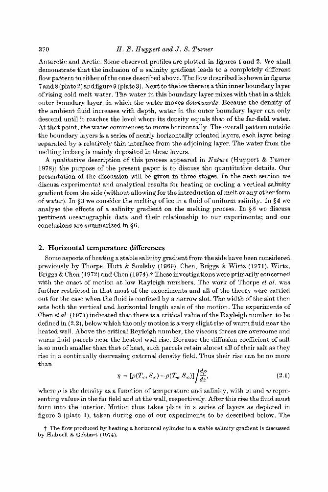
B I L ~ t<h 1 . 'l'wnlwrature (7') and salinity (S) profiles measured in the upper 400 m of the \Vedclcll Scd (at1,tf)ted froin figure 3 o f Foster B Carmack 1976). (a) NeaI the Scotia JAdge a t the northern ctlgr of thc wit. ( 0 ) Near the turnlng point of the curient gyre.

PIGUKE 2. Typical mean salinity profiles in the Arctic (Hellerman, private communication). (1) 772' N, 763" W, summer. (2) 67;' N, 60;" \V, summer. (3) 6'36" N, 6iF W, autumn.

relatively light layer above a deep, heavy layer of greater salinity. Neshyba then assumed that the amount of entrainment is determined by the criterion that the mixed fluid a t the top of the boundary layer has the same density as the surface water. Using this criterion, he calculated that, the entrainment ratio, the ratio of entrained water t o melt water, for Antarctic icebergs is approximately 60. This implies that the total upwelling around Antarctic icebergs is of the order of 1 0l1 m3 per day, which represents a considerable vertical transport.

The aim of this paper is t o show that another, and in our opinion more likely, mechanism pan occur. The essential feature of this mechanism is that it takes explicitly into account a variation of salinity with depth. Non-uniform vertical salinity distri- butions, either smooth or containing steps, are typical in most parts of both the

370 H . E. Huppert and J . S. Turner

Antarctic and Arctic. Some observed profiles are plotted in figures 1 and 2. We shall demonstrate that the inclusion of a salinity gradient leads to a completely different flow pattern to either of the ones described above. The flow described is shown in figures 7 and 8 (plate 2) and figure 9 (plate 3). Next to the ice there is a thin inner boundary layer of rising cold melt water. The water in this boundary layer mixes with that in a thick outer boundary layer, in which the water moves downwards. Because the density of the ambient fluid increases with depth, water in the outer boundary layer can only descend until it reaches the level where its density equals that of the far-field water. At that point, the water commences to move horizontally. The overall pattern outside the boundary layers is a series of nearly horizontally oriented layers, each layer being separated by a relatively thin interface from the adjoining layer. The water from the melting iceberg is mainly deposited in these layers.

A qualitative description of this process appeared in Nature (Huppert & Turner 1978); the purpose of the present paper is to discuss the quantitative details. Our presentation of the discussion will be given in three stages. In the next section we discuss experimental and analytical results for heating or cooling a vertical salinity gradient from the side (without allowing for the introduction of melt or any other form of water). In § 3 we consider the melting of ice in a fluid of uniform salinity. In § 4 we analyse the effects of a salinity gradient on the melting process. In $ 5 we discuss pertinent oceanographic data and their relationship to our experiments; and our conclusions are summarized in 9 6.

2. Horizontal temperature differences Some aspects of heating a stable salinity gradient from the side have been considered

previously by Thorpe, Hutt & Soulsby (1969), Chen, Briggs & Wirtz (1971), Wirtz, Briggs & Chen (1972) and Chen (1 974).t These investigations were primarily concerned with the onset of motion at low Rayleigh numbers. The work of Thorpe et al. was further restricted in that most of the experiments and all of the theory were carried out for the case when the fluid is confined by a narrow slot. The width of the slot then sets both the vertical and horizontal length scale of the motion. The experiments of Chen et al. (1971) indicated that there is a critical value of the Rayleigh number, to be defined in (2.2), below which the only motion is a very slight rise of warm fluid near the heated wall. Above the critical Reyleigh number, the viscous forces are overcome and warm fluid parcels near the heated wall rise. Because the diffusion coefficient of salt is so much smaller than that of heat, such parcels retain almost all of their salt as they rise in a continually decreasing external density field. Thus their rise can be no more than

7 = rP(T-9 8,) --P(T,,&)I Z’ (2.1) IdP where p is the density as a function of temperature and salinity, with 00 and w repre- senting values in the far field and a t the wall, respectively. After this rise the fluid must turn into the interior. Motion thus takes place in a series of layers as depicted in figure 3 (plate l ) , taken during one of our experiments to be described below. The

t The flow produced by heating a horizontal cylinder in a stable salinity gradient is discussed by Hubbell & Gebhart (1974).

Ice blocks melting into a salinity gradient 371

thickness of the layers scales with 7. The flow is towards the heated wall a t the bottom of each layer and away from the wall along the top. The layers slope gently upwards towards the wall because a t each interface inflowing fluid lies above outflowing fluid which is relatively hotter (due to the heat transfer from the wall) and saltier (due to its deeper origin). This is exactly one of the situations for which double-diffusive convec- tion occurs (Turner 1973, cha. 8) and heat is transferred upwards across the interface in preference to salt. The inflowing fluid hence decreases in density as it progresses to- wards the wall and has an upward component of motion. Using 7 as the vertical length to evaluate the Rayleigh number

where KT is the molecular diffusivity of heat, and using the (vertical) mean value of S,, Chen et al. determined from their experiments that the critical value of the Rayleigh number, R,, is 15 000 f 2500. Analysing the results of the nine experiments ranging in Rayleigh number from 14000 to 54000 for which layers occurred, they conclude that the thickness of the layers, h, expressed as a fraction of 4, is 0.81 0.10, with no syste- matic dependence on the Rayleigh number.

I n a number of different numerical calculations with R = lo5, Wirtz et al. (1972) and Chen (1974) obtained results in broad agreement with the experimental results.

Since the Rayleigh number calculated via (2.2) of an iceberg in polar seas is about it is of interest to determine the form of flow and layer scale for Rayleigh numbers

very much larger than critical. We thus conducted the following experiments. For the first of two series of experiments we centred a thin-walled, stainless steel circular cylinder of radius 44 cm and height 33 cm (a photographic developing cylinder, to be explicit) in a rectangular Perspex tank 40 x 20 x 30 cm high. The space between the cylinder and the container was filled with water a t room temperature, linearly strati- fied with salt, such that there was fresh water a t the surface. The filling was accom- plished using the standard double-bucket procedure first suggested by Oster & Yamamoto ( 1 963) and Oster ( 1 965). Hot water was then introduced into the cylinder and its temperature held constant by the use of a temperature controlled heating coil, known as a Thermoboy. Motions in the water were made visible by using a shadowgraph technique. The layer thicknesses were monitored during the experiments and frequent photographs were taken so that details of the experiments could be reconsidered later and analysed a t leisure.

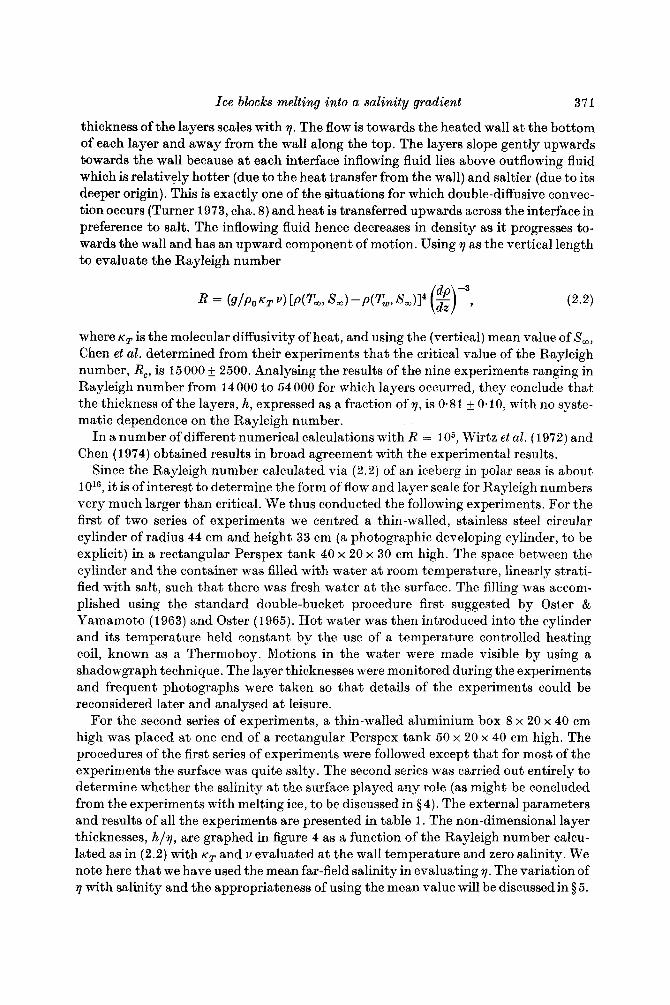
For the second series of experiments, a thin-walled aluminium box 8 x 20 x 40 cm high was placed a t one end of a rectangular Perspex tank 50 x 20 x 40 cm high. The procedures of the first series of experiments were followed except that for most of the experiments the surface was quite salty. The second series was carried out entirely to determine whether the salinity at the surface played any role (as might be concluded from the experiments with melting ice, to be discussed in 5 4). The external parameters and results of all the experiments are presented in table 1. The non-dimensional layer thicknesses, h / y , are graphed in figure 4 as a function of the Rayleigh number calcu- lated as in (2.2) with K~ and v evaluated a t the wall temperature and zero salinity. We note here that we have used the mean far-field salinity in evaluating 7. The variation of 7 with salinity and the appropriateness of using the mean value will be discussed in 3 5.

372 H . E . Huppert and J . S. Turner

TCU

("C) 21.7 21.1 22.5 22.3 22.0 24.7 20.9 21.1 22.7 23.2 25.0 20.2 21.2 21.5 22.6 21.1 21.2 22.4 23.7

17.8 18.8 16.5 17.3 17.6 15.2 16.4 17.2 17.8 18.0

~

Ttu ("C) 25.0 28.8 28.2 39.7 50.0 69.5 24.6 30.4 40.8 47.3 62-5 29.2 37.2 51.9 41.7 23.7 29.7 36.5 42.2

29.6 36.6 25.0 34.8 54.0 24.8 33-8 28.2 35.3 24.3

1 0 3 dp

Po dz --

(cm-I)

3.95 3.95 3.95 3.95 3.95 3-95 1.53 1.53 1.53 1-53 1.53 1.23 1.23 1.02 1.02 0.99 0.99 0.99 0.99

1.44 1.39 1.25 1.26 1-23 0.59 0.57 1.32 1-30 1.08

s, (%!J 63 63 63 63 63 63 33 33 33 33 33 25 25 43 43 25 25 25 25

41 41

106 104 105 156 155 181 181 37

h (cm) - 0.5 0.5 1.2 2.0 3.4 0.6 1.1 2,7 3-6 7.5 1.2 2.5 2.1 4.3 0.6 1.6 2.7 4.0

1.5 2.7 1.5 3.4 8.0 4.2 8.0 2.1 3.7 1.0

103 AP - Po

1.11 2.69 2.01 6.68

11-52 21.01

1.07 2.93 6-44 9.14

16.15 2.65 5,27 3-47 7.04 0.71 2.56 4.66 6.57

3.64 6.00 3.21 7.05

4.23 7.78 5.18 8.38 1.78

16.2

hlrl

- 0-73 0.98 0.71 0.69 0.64 0.86 0.57 0.64 0.60 0.7 1 0.56 0.58 0.62 0.62 0.84 0.62 0.57 0.60

0-59 0.63 0.58 0.6 1 0.61 0.59 0.59 0.53 0.57 0.58

R

1.9 x 103 7.0 x 1 0 4 2.1 x 104

3.2 x 107

2.7 x 104

4.7 x 1 0 7

3.2 x lo6

4.6 x lo8

1.7 x lo6

2.1 x 108 2.5 x lo8 2.2 x 106 3.9 x 107 1.2 x 107

2.0 x 104

4.6 x 1 0 7

2.3 x 10'

3.7 x 106

1.9 x 108

4.9 x 106

4.1 x lo6 1.1 x 108

1.2 x 108 1.8 x 108

2.0 x 108 5.9 x 106

4.5 x 107

4.4 x 1 0 9

2.5 x 107

TABLE 1. The experimental parameters and results of the experiments on heating a salinity gradient from the side. The results in the first group are from experiments conducted in the smaller container described in 92; those in the second group are from experiments in the larger container. There were no layers evident in the first experiment.

As the Rayleigh number increases from its critical value, h / y steadily falls from unity to a value of about 0-62 0-05 around R = 5 x 1 0 5 , whereafter it remains essen- tially constant. This is not in agreement with the stated conclusions of Chen et al. (197 I), but if their data are reconsidered, there is a definite suggestion of a decrease of h / y with increasing R, which is especially strong if the result from their last experi- ment, which was a t the largest Rayleigh number, is (somewhat arbitrarily) discarded. We conclude then that beyond a Rayleigh number of around lo5 the motion takes place in a series of layers of thickness 0.62 7 a t least up to a Rayleigh number of 1O1O and quite probably for much larger Rayleigh numbers.

We conducted another two series of experiments in which fluid with a constant salinity gradient was cooled at a vertical side wall rather than heated. In the first series, using the same tank and inner cylinder as in the first series of heating experi- ments, we attempted to keep the temperature spatially uniform a t 0°C within and a t the walls of the cylinder, by pouring in and gently stirring a brine solution in which

X

Ice blocks melting into a salinity gradient

#

# X I, 4 x x

373

X

+ +

0-2 0'41 01 I I I 1 I . I

104 105 1 O6 10' 108 109 10'0 R

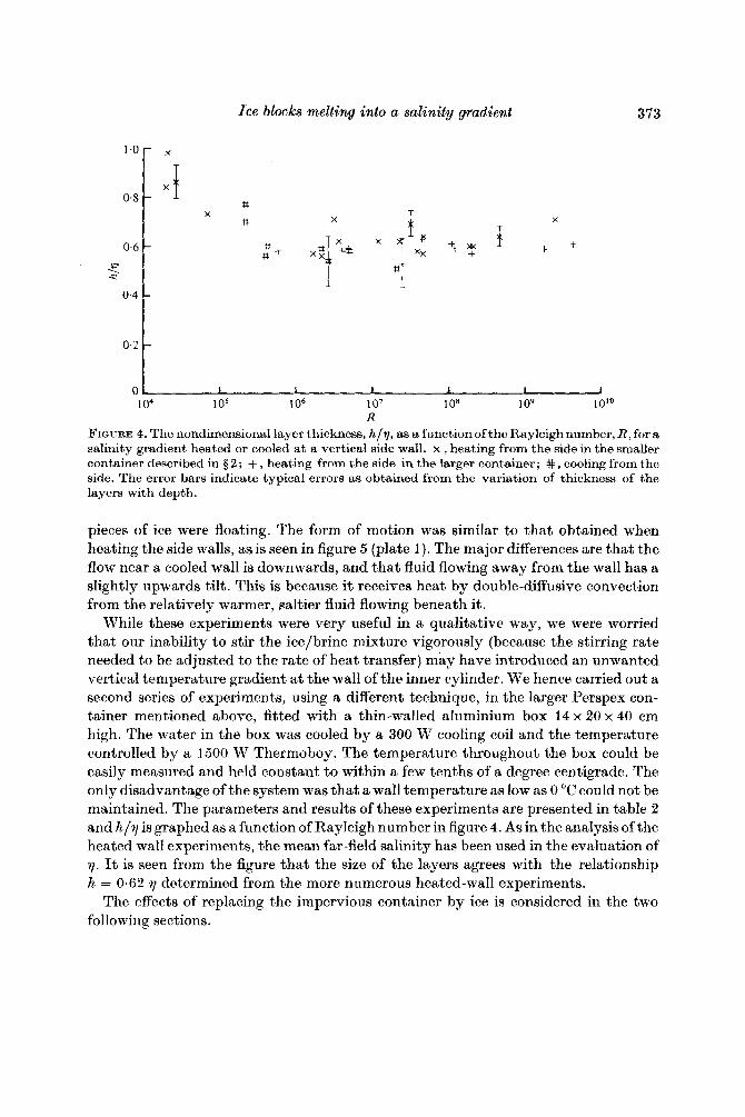
FIGURE 4. The nondimensional layer thickness, h / ~ , as a function of the Rayleigh number, R, for a salinity gradient heated or cooled a t a vertical side wall. x , beating from the side in the smaller container described in 3 2 ; + , heating from the side in the larger container ; # , cooling from the side. The error bars indicate typical errors as obtained from the variation of thickness of the layers with depth.

pieces of ice were floating. The form of motion was similar to that obtained when heating the side walls, as is seen in figure 5 (plate 1) . The major differences are that the flow near a cooled wall is downwards, and that fluid flowing away from the wall has a slightly upwards tilt. This is because it receives heat by double-diffusive convection from the relatively warmer, ealtier fluid flowing beneath it.

While these experiments were very useful in a qualitative way, we were worried that our inability to stir the ice/brine mixture vigorously (because the stirring rate needed to be adjusted to the rate of heat transfer) may have introduced an unwanted vertical temperature gradient a t the wall of the inner cylinder. We hence carried out a second series of experiments, using a different technique, in the larger Perspex con- tainer mentioned above, fitted with a thin-walled aluminium box 14 x 20 x 40 em high. The water in the box was cooled by a 300 W cooling coil and the temperature controlled by a 1500 W Thermoboy. The temperature throughout the box could be easily measured and held constant to within a few tenths of a degree centigrade. The only disadvantage of the system was that a wall temperature as low as 0 "C could not be maintained. The parameters and results of these experiments are presented in table 2 and h/T is graphed as a function of Rayleigh number in figure 4. As in the analysis ofthe heated wall experiments, the mean far-field salinity has been used in the evaluation of T. It is seen from the figure that the size of the layers agrees with the relationship h = 0.62 7 determined from the more numerous heated-wall experiments.

The effects of replacing the impervious container by ice is considered in the two following sections.

374 H . E. Huppert and J . S. Turner

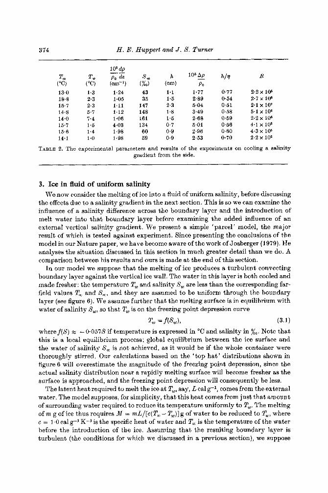
103 dp -- Tea T w Po dz 8, h 1 0 ' 9 h/q R

("C) ("(2) (cm-l) (%J (em) Po 13.0 1.3 1.24 43 1.1 1.77 0.77 2.2 x 106 18.8 2.3 1.05 35 1-5 2-89 0.54 2.7 x 106 15.7 2.3 1.11 147 2.3 5.04 0.51 2.1 x 107 14.8 5.7 1.12 148 1.8 3.49 0.58 5.1 x loE 14.0 7.4 1.06 161 1.5 2-68 0.59 2.2 x 106 15.7 1.5 4.03 134 0.7 5.01 0.56 4.1 x lo6 15.6 1.4 1.98 60 0.9 2.96 0.60 4.3 x 106

2.2 x 106 14.1 1.0 1.98 59 0.9 2.53 0.70

TABLE 2. The experimental parameters and results of the experiments on cooling a salinity gradient from the side.

3. Ice in fluid of uniform salinity We now consider the melting of ice into a fluid of uniform salinity, before discussing

the effects due to a salinity gradient in the next section. This is so we can examine the influence of a salinity difference across the boundary layer and the introduction of melt water into that boundary layer before examining the added influence of an external vertical salinity gradient. We present a simple 'parcel ' model, the major result of which is tested against experiment. Since presenting the conclusions of the model in our Nature paper, we have become aware of the work of Josberger (1979). He analyses the situation discussed in this section in much greater detail than we do. A comparison between his results and ours is made a t the end of this section.

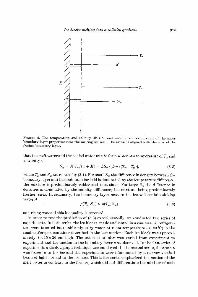
I n our model we suppose that the melting of ice produces a turbulent convecting boundary layer against the vertical ice wall. The water in this layer is both cooled and made fresher: the temperature T, and salinity S, are less than the corresponding far- field values T, and S,, and they are assumed to be uniform through the boundary layer (see figure 6) . We assume further that the melting surface is in equilibrium with water of salinity S,, so that T, is on the freezing point depression curve

Tw = f(SA (3.1)

where f ( S ) x - 0.057s if temperature is expressed in "C and salinity in x0. Note that this is a local equilibrium process; global equilibrium between the ice surface and the water of salinity S, is not achieved, as it would be if the whole container were thoroughly stirred. Our calculations based on the 'top hat ' distributions shown in figure 6 will overestimate the magnitude of the freezing point depression, since the actual salinity distribution near a rapidly melting surface will become fresher as the surface is approached, and the freezing point depression will consequently be less.

The latent heat required to melt the ice a t T,, say, L cal g-l, comes from the external water. The model supposes, for simplicity, that this heat comes from just that amount of surrounding water required to reduce its temperature uniformly to T,. The melting of m g of ice thus requires M = mL/[c(T, - T,)] g of water to be reduced to T,, where c = 1.0 cal g-l K-l is the specific heat of water and T, is the temperature of the water before the introduction of the ice. Assuming that; the resulting boundary layer is turbulent (the conditions for which we discussed in a previous section), we suppose

Ice blocks melting into a salinity gradient 375

t FIGURE 6. The temperature and salinity distributions used in the calculation of the inner boundary-layer properties near the melting ice wall. The arrow is aligned with the edge of the fresher boundary layer.

that the melt water and the cooled water mix to form water a t a temperature of T, and a salinity of

(3.2)

where T, and S, are related by (3.1). For small S , the difference in density between the boundary layer and the undiluted far field is dominated by the temperature difference; the mixture is predominately colder and thus sinks. For large S, the difference in densities is dominated by the salinity difference; the mixture, being predominately fresher, rises. I n summary, the boundary layer next to the ice will contain sinking water if

(3.3)

S, = MS,/(m + M ) = LS,/[L + c(T, - T,)],

P(T,, S,) > P ( G , 8,)

and rising water if this inequality is reversed. In order t o test the prediction of (3.3) experimentally, we conducted two series of

experiments. I n both series, the ice blocks, made and stored in a commercial refrigera- tor, were inserted into uniformly salty water a t room temperature ( N" 20 "C) in the smaller Perspex container described in the last section. Each ice block was approxi- mately 3 x 15 x 20 cm high. The external salinity was varied from experiment to experiment and the motion in the boundary layer was observed. I n the first series of experiments a shadowgraph technique was employed. In the second series, fluorescein was frozen into the ice and the experiments were illuminated by a narrow vertical beam of light normal to the ice face. This latter series emphasized the motion of the melt water in contrast to the former, which did not differentiate the mixture of melt

376 H . E. Huppert and J . X. Turner

water and external water. The conclusion from both series was nevertheless the same. Using the density tables contained in the International Critical Tables, with (3.1)

and ( 3 . 2 ) , we calculate that with T = 20°C the change over between upward and downward moving water in the boundary layer should occur a t a salinity of IS%,, or an external density of 1.010 g 0111-3. Evaluating densities by using a refractometer, we found that in the shadowgraph experiments a downward motion occurred up to an external density of 1-01 1 g em-3 and an upward motion beyond an external density of 1.013 g em-3. In the experiments using fluorescein, downward motion occurred up to an external density of 1.011 g ~ m - ~ , the motion had an extremely emall upward component a t an external density of 1.012 g ~ m - ~ and upward motion was observed beyond an external density of 1.017 g ~ m - ~ . These results are seen to be in good general agreement with the simple theory presented a t the beginning of this section. We conclude by emphasizing that no evidence of layering or strong horizontal motions was seen in any of the experiments.

To turn now to Josberger’s (1979) experiments, he concludes that a t external temperatures less than approximately 25OC the flow near the bottom of the ice is laminar with a rising inner layer and a sinking outer layer. Above a height which is only a few centimetres under laboratory conditions this flow becomes turbulent. For low external salinities the turbulent flow is predominantly downwards; for higher external salinities i t is predominantly upwards. At larger external temperatures Josberger observed that the short laminar layer was a t the top of the ice. Josberger’s criterion for the salinity a t which the changeover between upward and downward motion occurs in the turbulent flow leads to results comparable with those obtained from (3 .3) . The results are not identical, both because of the different approaches employed and because Josberger’s criterion is based on the net buoyancy integrated across the boundary layer, while our criterion is based on the density a t the wall. With the extra understanding gained by studying Josberger’s results, we see that in our experiments we concentrated on the turbulent flow against the face of the ice block and neglected the short laminar region.

4. Melting ice in a salinity gradient To investigate the effects of melt water on the boundary layer, we carried out a

series of experiments of meIting ice bIocks in a salinity gradient. We tried to encompass as wide a range of parameters as possible in our laboratory setting, carrying out experiments with different salinity gradients, surface salinities and a range of far- field temperatures. The parameters for all the experiments are presented in table 3. For most of the experiments, the smaller Perspex container described in § 2 was filled to a depth of nominally 26 cm with water linearly stratified with salt by the mechanism mentioned previously. Measurements of the density were obtained, with a refracto- meter, to within an accuracy of 10-4 g ~ m - ~ , throughout the depth of the water a t an interval of 2-0 cm. By fitting a straight line through these data points, the mean density gradient could be accurately determined. (The correlation coefficient for the linearity of the data was typically larger than 0.998.) An ice block made from water which had been previously deaerated under a vacuum and measuring 15 x 3 x 20 cm high was inserted carefully into the water with its largest two faces vertical and the top of the ice block just beneath the surface of the water. All the experiments were

Ice blocks melting into a salinity gradient 377

T, ("0 21.6 23.0 21.9 22.5 21.0 22.5 20.8 23.1 21.2 22.3 21.0 23.8 21.8 10.5 8.0

13-0 12.0 12.0 14.5 25.0 23.0 22.0 26.0 23.0 20.5 22.0

9.0 21.0 23.0

10s dp

(cm-l)

6.02 5.84 3.85 2.34 2.03 2.03 1.96 1.85 1.12 0.86 0.71 0.62 0.49 1.86 0.66 1.37 1.24 1.32 1-18 0.44 0.59 0.55 0-65 0.37 1.78 1.98 0.67 0.55 1.81

-_ Po dz 8,

i %o)

92 93 61 38 34 32 30 36 17 19 14 14 08 80 95 85 83 81 80 15 18 16 17 13

103 101 100 130 178

h (em)

0.7 0.8 0.9 1.2 1 *2 1.3 1.1 1 *3 1.8 2-3 2.5 3.4 4.1 0.9 1-6 1.5 1.6 1-4 1.7 5.8 3.1 3.2 4.0 6.0 1 *4 1.6 1.5 3.9 1.6

10s Ap

Po 6-37 6-94 5.13 4.20 3.59 3.90 3.32 4.26 2.75 3.15 2.58 3-29 2.45 2,28 1.90 3.13 2.77 2.72 3.45 3.68 3.29 2.92 4-10 2.99 6.39 6.88 2.28 7.50 9.75

- hlT

0.66 0.67 0.68 0.67 0.68 0.68 0.65 0.56 0.73 0.63 0.69 0.64 0.82 0.73 0.56 0-66 0.72 0.68 0.58 0.69 0.56 0.60 0.63 0-74 0.39 0.46 0.44 0.29 0.30

R

3.1 x lo6 4.8 x 10' 6-0 x 10' 1.0 x 108

1.1 x 108

2.1 x 108 1.7 x 10' 6.4 x 10' 5.1 x loe

8.2 x 105

6-7 x 105

2.0 x 1 0 7

1.3 x 107 1.7 x 10' 1.9 x 108 1.5 x 10' 1-3 x 10' 9.8 x 10' 3.6 x 10' 8.9 x 107 2.4 x 107 1.8 x 107 4.2 x 107 6.5 x 1 0 7 1.2 x 107 1.2 x 107

6.3 x 107

3.7 x 10' 7.8 x 10'

TABLE 3. The experimental parameters and results of the experiments on iceblocks melting into a salinity gradient. The last five cases are exceptional, being at large Rayleigh numbers and high salinities.

viewed using the shadowgraph technique, and in some of these up to six layers of dye were introduced into the water a t different levels during the filling process. The pur- pose of the dye was to allow us to ascertain the transport and final position of the ambient water, and in particular to test the prediction of Neshyba (1977) that large amounts of ambient water would be entrained in a rising turbulent boundary layer. For some experiments a minute quantity of fluorescein was frozen uniformly into the ice block. This allowed us to observe the motion of the melt water, as distinct from the ambient water or the melt-water/ambient-water mixture. I n a different group of experiments, we used an ice block into which had been frozen just a thin horizontal line of fluorescein, thus allowing us to ascertain the final position of melt water origi- nating a t a specific depth.

The results of all the experiments were qualitatively the same. Further, the data we obtained can be interpreted in a quantitative fashion with only minor modification of the analysis already presented, except for a few experiments a t extreme parameter values well beyond those appropriate to oceanographic conditions. VC'e will describe

378 H . E . Huppert and J . 8. Turner

the general pattern first, qualitatively and quantitatively, and then explain the exceptional cases.

In the immediate vicinity of the ice block, the cold melt water leads to a flow very much like that produced when an ice block is inserted in water of uniform salinity, as described in the previous section. The flow is upwards a t levels where the external salinity is greater than about 16 x0 and downwards at levels above this. Such a change-over point did not exist in all the experiments and would not exist under typical oceanographic conditions (where the flow in this thin boundary layer would always be upwards). This cold, relatively fresh boundary layer is turbulent, as is the flow in the external fluid, and the interchange between them allows a small fraction of fresh water to be added to the external flow (as described further in the next sec- tion). For the present purpose, however, we can regard the inner boundary layer as providing an effective temperature boundary condition of T, on the fluid of salinity S , just outside it (cf. figure 6, and the argument leading to (3.2)). Temperature measurements taken from thermistors frozen in the ice indicate that a t the warm far-field temperatures employed in these experiments the temperature of the ice is in fact approximately 0 "C. This is because the influx of melt water into the inner bound- ary layer lowers the salinity by a sufficiently large amount that the freezing point depression is negligible. At lower external temperatures the melt rate is lower, the inner layer is more salty and the temperature of the ice is closer to Tfp, the freezing point depression a t the far-field salinity. This will be discussed further in $5.

With an effective boundary condition of 0 "C and S , the ambient water is under the influence of cooling from the side, exactly as described in $2 . The flow pattern is as depicted in figures 7 and 8 (Plate 2) and figure 9 (plate 3). Ambient water flows in- wards towards the ice, is cooled to approximately 0 "C, sinks a distance which scales with 7 (with T, = 0) and then turns back into the interior above relatively warmer, saltier water. During this past part of the motion, double-diffusive heat transfer takes place and the water is warmed slightly and thus rises. The inward flow of the water, as yet uninfluenced by melt water, takes place in the dark sectors interleaving the bright layers in figure 8 and is responsible for the corresponding horizontal V-shaped sectors in the shadowgraph pattern of figure 7. Most of the melt water flows into the exterior within two or three layer depths above where it was formed. Very little reaches the surface, as is seen in figure 9. In those experiments in which the ambient water was dyed, the dye sloped downwards within three or four centimetres of the ice and was transported by double-diffusive convection across the interfaces into only the adja- cent layers. This further confirms the downward motion of the ambient water and also calls into question the large entrainment and upward transport of ambient water predicted by Neshyba.

The layer size h as a function of the imposed density difference and the salinity gradient is presented in figures 10 and 11. Figure 10 plots the values of

against dp/dz for the 29 experiments, using, as before, the vertical mean value of S,. Among the 29 data points are 5 which are the exceptional cases we mentioned earlier in this section and which will be discussed in the next paragraph. Also drawn on figure 10 is the best-fit straight line of slope - 1 through all the data points except the

Ice blocks melting into a salinity gradient 379

5 x 103

2 x 103 h

5

4 K!

, 5 x 102

4 0-

p" 2 x 102

v - 103

v Q

h

v P L . -s

102

5 x 10' I I I I I I

lo4 2 x 10-4 5 x 10-4 10-3 2 x 10-3 5 x 10-9 10-2

PO' - dp (cm-1) dz

FIGURE 10. The layer thickness per unit density difference, h/[p(O, 8,) -p(T, , S,)],asafunction of the density gradient, dp/dz, for ice blocks melting into a salinity gradient. The results of the five exceptional experiments a t large Rayleigh number and high salinities are denoted by A to differentiate them from the results of the twenty-four standard experiments denoted by x . The error bars were obtained as indicated in the caption to figure 4. The straight line is the best fit with slope - 1 to the data of the twenty-four standard experiments.

5 exceptional ones. We conclude that the layer thickness is given by

h = (0.66 5 0.06) [p(O, 8,) -p(T,,8m)]/$.

The change in density due to using 0°C instead of T, is entirely negligible in our experiments carried out with T, near room temperature. Figure 11 presents the values of h/T as a function of the Rayleigh number defined as in (2.2) with T, = 0 and K~ and v evaluated at zero temperature and zero salinity. As in the previous situation of heating or cooling a salinity gradient from the side, we find that there is no systematic Rayleigh number dependence.

The exceptional cases which do not fit the above quantitative analysis are those for which both the Rayleigh number and mean salinity are large. The large Rayleigh number indicates that the convection near the ice is very vigorous and that mixing between the external fluid and the boundary layer near the ice is enhanced. The mix- ing decreases the effective salinity as seen by the external fluid and its influence increases with the far-field salinity. A relatively small decrease in salinity due to the mixing is sufficient to change the results of the five exceptional cases so as to be in line with the others. The small change required is seen by defining for the last two entries

380 H . E . Huppert and J . S. Turner

r

"'tl I

0.4 '

0.2 .

A f T T

01 I I I I I 1 104 10s 1 O6 107 108 109 10'0

R FIGURE 11. The non-dimensional layer thickness, hlq, as a function of the Rayleigh number, R, for ice blocks melting into a salinity gradient. The same symbols have been used as in figure 10.

of table 3, the effective salinity, s", such that

Such calculations indicate that s" is reduced from the mean far-field salinity, S,, by less than 3 yo of its value. Note again that this is a change in the external salinity, caused by the mixing of fresh water outwards, across the edge of the fresher boundary layer shown in figure 6. It is not the same process as the inward entrainment considered in 3 Sand earlier in this section, and it is not important a t lower salinities. In particular, oceanographic salinities are well within the range for which (4.1) is appropriate.

5. Discussion A number of different aspects of our experiments, their interpretation and their

application to oceanographic situations will now be considered, before presenting the major conclusions of the study in the final section. For all the experiments the layer thicknesses reported in tables 1-3 were obtained by evaluating the average thickness of all the observed layers, which varied in number between 6 and about 50. For a large number of the experiments there was no systematic variation of layer scale with depth and the evaluation of the average thickness, rather than a local value, smoothed out the effects of random variations. Such variations were typically small and were the major contributors to the error bars displayed on figures 4, 10 and 11. It is con- sistent with this evaluation of the average thickness to compare the results with a vertically averaged theory, or to be explicit, to use the average far-field salinity in the calculation of 7; and we have done so.

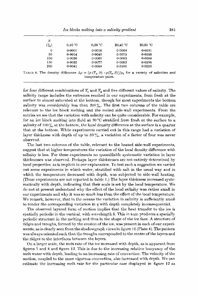
This having been said, it is essential to estimate the variation which would arise if y were evaluated a t the local far-field salinity. Typical variations can be determined from table 4, which presents values of

[P(Tl> 8) -P(T,, S) l lP,

Ice blocks melting into a salinity gradient 381

s (%J 0,lO "C 0,20 "C 20,40 "C 20,60 "C

0.0151 50 0.0014 0.0040 0.0073 0.0168

100 0.0026 0.0061 0.0083 0.0184 150 0.0035 0.0077 0.0092 0.0198 200 0.0041 0.0088 0*0101 0.0210

TABLE 4. The densit,y difference A p = [p (TI, 8)-p(T,, S)] /p , for a variety of salinities and temperature pairs.

0 0~0001 0.0016 0.0060

for four different combinations of TI and T2 and five different values of salinity. The salinity range includes the extremes reached in our experiments, from fresh a t the surface to almost saturated a t the bottom, though for most experiments the bottom salinity was considerably less than 200%,. The first two columns of the table are relevant to the ice block melting and the cooled side-wall experiments. From the entries we see that the variation with salinity can be quite considerable. For example, for an ice block melting into fluid a t 20°C stratified from fresh a t the surface to a salinity of 100 x0 a t the bottom, the local density difference a t the surface is a quarter that a t the bottom. While experiments carried out in this range had a variation of layer thickness with depth of up to 50 yo, a variation of a factor of four was never observed.

The last two columns of the table, relevant to the heated side-wall experiments, suggest that a t higher temperatures the variation of the local density difference with salinity is less. For these experiments no quantifiable systematic variation in layer thicknesses was observed. Perhaps layer thicknesses are not entirely determined by local properties, as is implicit in our explanation. To test such a suggestion we carried out some experiments'in which water, stratified with salt in the usual way and in which the temperature decreased with depth, was subjected to side-wall heating. (These experiments are not reported in table 1 .) The layer thickness increased syste- matically with depth, indicating that their scale is set by the local temperature. We do not a t present understand why the effect of the local salinity was rather small in our experiments and why it was so much less than the effect of the local temperature. We remark, however, that in the oceans the variation in salinity is sufficiently small to render the corresponding variation in 7 with depth completely inconsequential.

The observed layered form of motion implies that the heat transfer t o the ice is spatially periodic in the vertical, with wavelength h. This in turn produces a spatially periodic structure in the melting and thus in the shape of the ice face. A structure of ridges and troughs, formed by the erosion of the ice, was present in each of our experi- ments, as is clearly seen from the shadowgraph views in figure 12 (Plate 4). The pattern was always oriented such that the troughs corresponded to the centre of the layers and the ridges to the interfaces between the layers.

On a larger scale, the melt rate of the ice increased with depth, as is apparent from figures 7 and 8 and figure 12. This is due to the increasing relative buoyancy of the melt water with depth, leading to an increasing rate of convection. The velocity of the motion, coupled to the more vigorous convection, also increased with depth. We can estimate the increasing melt rate for the particular case displayed in figure 12 as

382 H . E. Huppert and J . S . Turner

follows. By subtracting the volume of the ice at the level of the fourth layer from the bottom, as measured by the area between the two top interfaces in figure 12 (b ) , from that determined in the same manner from figure 12 (a ) , we obtain the volume of ice melted a t that level. Repeating this procedure for the level of the bottom layer, we find that the melt rate per unit area a t the depth of the bottom layer is 25 yo larger than that at the depth of the fourth layer.

The mechanism responsible for mixing a small fraction of melt water out into the extending layers requires further discussion. The observed outward transfer implies that the outer flow is turbulent; otherwise, there could only be entrainment inwards into the upward-flowing fresher layer against the ice. The turbulence in the layers is due to double-diffusive convection, produced by the buoyancy flux across the diffu- sive interfaces (which has previously been referred to in explaining the tilt of the layers as they move outwards). The stratification in the 'finger' sense within each layer can also produce strong local convection in recirculating regions just outside the inner boundary layer. This is seen clearly in time-lapse films of the layer formation and is visible in figures 8 and 12.

The extension of our results on the layer scales to the ocean is clearly both tempting and desirable. We do so now, making the assumption that our results can be carried over to the ocean, where the far-field temperature is significantly less than in our experiments. A series of experiments to investigate the validity of this assumption has already been carried out and the details will be reported elsewhere (Huppert & Josberger 1980). A summary of the conclusions is that a t low far-field temperatures the form of motion is exactly as described above for melting into warm water, and that the scale of the layers is well represented by the same relationship as quoted in the abstract with T, = Ttp, the freezing point depression a t the far-field salinity. This may again be regarded as a consequence of the general relation (3.2) with S, + S , because T, and T, are nearly equal. The application of our results to the lower temperatures found in polar seas thus seems justifiable.

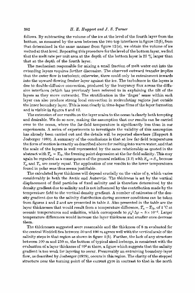
The calculated layer thickness will depend crucially on the value of q, which varies considerably in both the Arctic and Antarctic. The thickness is set by the vertical displacement of fluid particles of fixed salinity and is therefore determined by the density gradient due to salinity and is not influenced by the contribution made by the temperature field to the vertical density gradient. A number of estimates of the den- sity gradient due to the salinity distribution during summer conditions can be taken from figures 1 and 2 and are presented in table 5 . Also presented in the table are the layer thicknesses that would result from a temperature difference, T, - Tpp, of 1 "C at oceanic temperatures and salinities, which corresponds to p i 1 A p - 5 x Larger temperature differences would increase the layer thickness and smaller ones decrease them.

The thicknesses suggested seem reasonable and the thickness of 8 m evaluated for the central Weddell Sea between 50 and 100 m agrees well with the vertical scale of the salinity steps in that region as shown in figure I ( b ) . Further, the lack of any structure between 100 m and 250 m, the bottom of typical sized icebergs, is consistent with the evaluation of a layer thickness of 103 m there, a figure which suggests that the salinity gradient is too weak for layering to occur. Presumably an entraining boundary-layer flow, as described by Josberger (1979), occurs in this region. The clarity of the stepped structure near the turning point of the current gyre in contrast to that in the north

Ice blocks melting into a salinity gradient 383

Location

(i) North Weddell Sea, 100-200 m 1 x 10-6 30 (ii) Central Weddell Sea, 60-100 m 4 x 10-6 8

(iii) Central Weddell Sea, 100-400 m 5 x 10-8 10s (iv) Arctic, 0-30 m 3 x 10-6 1 (v) Arctic, 30-100 m 6 x lo-@ 5

TABLE 5 . Density gradients and predicted layer thickness in various polar areas.

Weddell Sea may be caused by the fact that individual icebergs spend more time in the former, more slowly moving region. Unfortunately, there are as yet too little data in either the Arctic or Antarctic to make more definite statements.

We conclude this section by briefly discussing two as yet unresolved aspects of iceberg melting, starting with the effects of a moving iceberg. It is commonly accepted that icebergs drift with the prevailing currents, little influenced by the wind, and that the relative motion between ice and water is small. A significant vertical shear in the velocity must to some extent alter this conclusion, but this effect too can only be quantified by detailed measurements close to icebergs. About 7 yo by volume of an Antarctic iceberg is compressed air. During the melting process this air is released as bubbles in the inner boundary layers. This increases the upward buoyancy in the inner layer, which does not however alter the dynamics of the downward flowing ambient fluid. The bubble release may alter the intensity of the convection and the melting rate; it may also carry some of the melt water to slightly higher levels, but it is unlikely to influence the overall nature of the outer flow field or the thickness of the layers, which as our experiments have shown are determined mainly by the tempera- ture difference.

6. Conclusions Our experiments and the related theoretical explanation of them indicate that the

water originating from ice melting in fluid stratified with salt undergoes relatively little vertical displacement. The melt water flows out of a thin vertical boundary layer near the ice into a series of almost horizontal layers set up in the ambient field. The thickness of the layers is relatively uniform throughout the depth of the fluid, and is given by

= 0.65 [P(T,, 8,) -P(T,, S,)l 1: - *

In the general case, T, is the depressed freezing point corresponding to the salinity S, in the fresher convecting boundary layer next to the melting ice, which can be estimated from (3.1) and (3.2). I n our experiments a t room temperature, and in the ocean under tropical conditions, T, may be taken as 0 "C without causing a significant change in the estimate of the horizontal density difference. Thus the form of the flow in the layers is the same as that which results when a stratified fluid is bounded by a vertical side wall uniformly maintained a t T, z 0 "C. At temperatures near the freezing point, the appropriate limit is T, z Tip, the depressed freezing point corresponding to

3 84 H . E . Hu,ppert and J . S . Turner

the salinity S,. The addition of melt water has little effect on the dynamics of the outer layers in either case. The extrapolation of our results to smaller salinity grad- ients suggests a typical layer thickness of between 10 and 30 m for Antarctic values of the density gradient. A thickness of only a few metres is euggested for representative Arctic density gradients. Observations in polar seas are not sufficient to test our ideas, and we close with a plea for more measurements to be made.

We are indebted to Gordon Robin and Charles Swithinbank for their encourage- ment during this work, to Joyce Wheeler for analysing some of the data and preparing the figures and to Ross Wylde-Browne for his superb aid in performing the experi- ments, especially with the photography. The work was initiated while one of us (HEH) was a Visiting Fellow at The Australian National University. He gratefully acknowledges the support received from that University and from The Royal Society. Additional support was received from the Ministry of Defence (Procurement Execu- tive), The Natural Environmental Research Council and from the National Science Foundation under grants ENG 75-02985 and ENG 77-27398.

REFERENCES

CHAPMAN, A. J. 1960 Heat Transfer. MacMillan. CHEN, C. F. 1974 Onset of cellular convection in a salinity gradient due to a lateral temperature

gradient. J . Fluid Mech. 63, 563-576. CHEN, C. F., BRIGGS, D. G. & WIRTZ, R. A. 1971 Stability of thermal convection in a salinity

gradient due to lateral heating. Int . J . Heat Mass Transfer 14, 57-65. FOSTER, T. D. & CARMACK, E. C. 1976 Temperature and salinity structure in the Weddell Sea.

J . Phys. Oceanog. 6, 36-44. HUBBELL, R. H. & GEBHART, B. 1974 Transport processes induced by a heated horizont,al

cylinder submerged in quiescent, salt-stratified water, Proc. 1974 Heat Transfer and Fluid Mechanics Institute, pp. 203-2 19.

HUPPERT, H. E. & JOSBERGER, E. G. 1980 The melting of ice in cold stratified water. J . Phys. Ocennog. (to appear).

HUPPERT, H. E. & LINDEN, P. F. 1979 On heating a salinity gradient from below. J . Fluid Mech. 95, 431-464.

HUPPERT, H. E. & TURNER, J. S. 1978 On melting icebergs. Natzrre 271, 46-48. JOSBERGER, E. G. 1979 Laminar and turbulent boundary layers adjacent to melting vertical

ice walls in salt water. Ph.D. thesis, Department of Oceanography, University of Washing- ton.

NESHYBA, S. 1977 Upwelling by icebergs. Nature 267, 507-508. OSTER, G. 1965 Density gradients. Scienti$c American 213, 70-76. OSTER, G. & YAMAMOTO, M. 1963 Density gradient techniques. Chem. Rev. 63, 257-268. THORPE, S. A., HUTT, P. K. & SOULSBY, R . 1969 The effects of horizontal gradients on thermo-

TURNER, J. S . 1973 Buoyancy Effects in Fluids. Cambridge University Press. WIRTZ, R. A., BRIGGS, D. G. & CHEN, C. F. 1972 Physical and numerical experiments on

haline convection. J . Fluid Mech. 38, 375-400.

layered convection in a density stratified fluid. Geophys. Fluid Dyn. 3, 265-288.

Jousnul of Fluid Mechanics, Vol. 100, part 2 Plate 1

FIGURE 3. A salinity gradicnt heated from the side, through a central metal cylinder. Depth of water 26 em; specific gravity a t bottom 1.044 and a t top 1-017; T, = 21.5 "C, T, = 31.9 "C. Photograph taken 74 minutes after heating was begun. Note the downward tilt of thc layers as they extend away from the wall.

FIGURE 5. A salinity gradient cooled from the side, through a central metal cylinder. Depth of water 26.5 cm; specific gravity a t bottom 1.027 and a t top 1.000; T, = 21.4 "C, nominal tem- perature of inner cylinder 0 "C. Photograph taken 8 minutes after brine and ice mixture was added to the central cylinder. Note the upward tilt of the layers as they extend outwards, and the slow downward transport of dye from an originally horizontal layer of dye put into the tank during filling.

HUPPERT AND TURNER (Facing p . 384)

Journal of Fluid nlechanics, Vol. 100, part 2 Plate 2

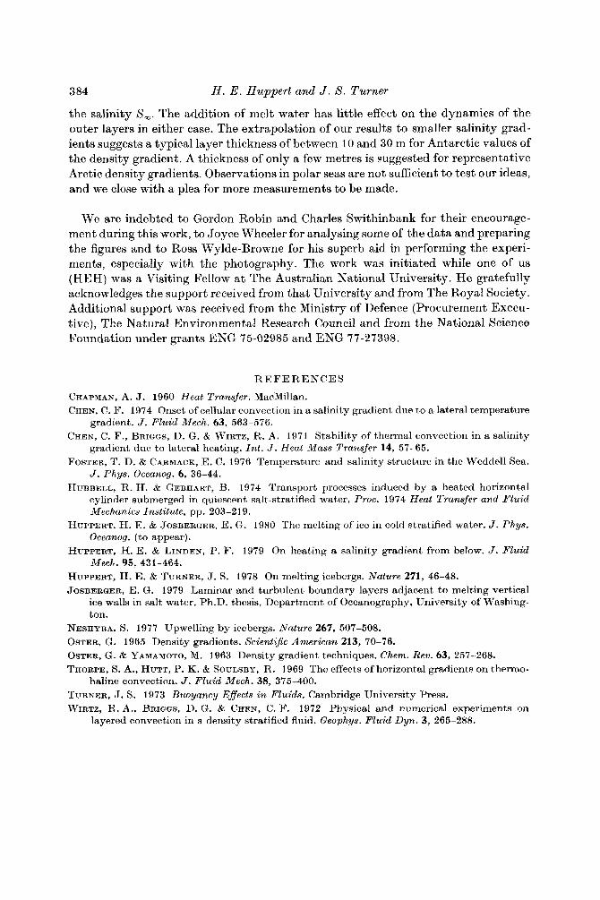
FIGURE 7 . Shadowgraph photograph of ice melting into a salinity gradient, showing thp turbu- lent boundary layer against the block, the tilted extending layers, and the downward distortion of dye layers placed in the tank during filling. Depth of water 25 cm; specific gravity a t bottom 1.052 and a t top 1 000; T, = 22.5 "C, T,, = 0 "C. Photograph at 8 min 42 s aftw mrerting iceblocak.

FIGURE 8. Ice melting into a salinity gradient. A small amount of fluorescein has been frozen into the ice just under the surface, and the extending layers are illuminated from the side. Specific gravity at, bottom 1.025 and a t top 1.000; depth 28 cm; T% h 22 "C. Note t,he more intense dye patches which mark recirculating regions near the block in several of the layers.

HUPPERT AND TURKER

Journal of Fluid Nechanics, Vol. 100, purt 2 Plate 3

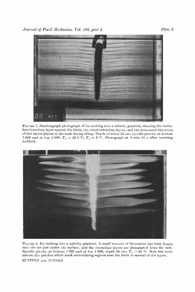
FIGURE 9. Ice molting into a salinity gradient with fluorescein frozen into the block, as in t,he experiment shown in figure 7. Depth of water 26 em; specific gravity a t bot)tom 1.060 and at top 1.000; Tv, = 22.5 "C, T, = 0 "C. ( a ) 15 minutes after inserting the ice block, showing the distri- bution of the meltwater as marked by the dye. (b) 25 minutes aft.er the start of the experiment,, and shortly after the ice block has been carefnlly removed. The volnmc of tlyetl water is much greater than that, of the ice block, indicating that the melt water has mixed with a large volume of salty watcr anti has spread out close to the level at, which is produced; 1it)tle reaches the surface.

HUPPERT AND TURNER

Journal of Fluid Mechanics, Vol. 100, part 2 Plate 4

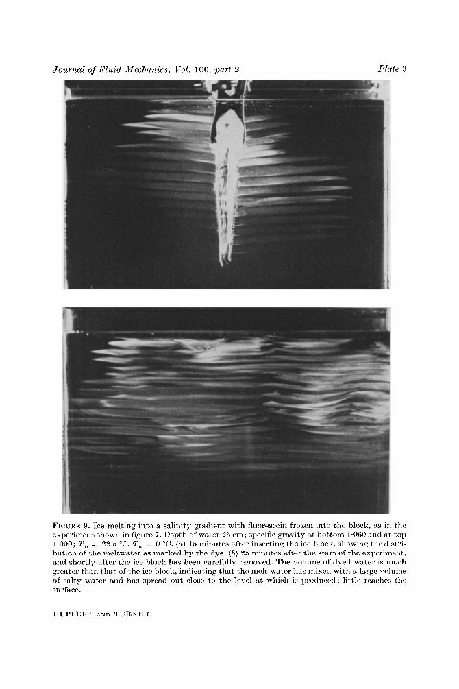
FIGURE 12. The effect of convection in layers on the rate of melting of an ice block in a salinity gradient. Depth of water 25 em; specific gravity at bottom 1.011 and at top 1.000; T, = 21.8 "C, T , = 0 "C. A series of ridges is produced a t the level of the interfaces with troughs corresponding to the centres of the layers. The two photographs were taken at approximately (a ) 10 minutes and ( 6 ) 15 minutes after insertion of the ice. Note the extra layers visible below the block, which have been formed by the process of cooling the salinity gradient from above. The inverse situa- tion, heating a salinity gradient from below, involves exactly the same physics and has been extensively investigated by Huppert & Linden (1979).

HUPPERT AND TURNER