INNOVATION DIFFUSION IN GEOGRAPHIC 

INFORMATION SCIENCE RESEARCH

THESIS

Presented to the Graduate Council ofTexas State University­San Marcos

in Partial Fulfillmentof the Requirements

for the Degree

Master of SCIENCE

by

David A. Parr, B.S.

San Marcos, TexasJune 2008

INNOVATION DIFFUSION IN GEOGRAPHIC 

INFORMATION SCIENCE RESEARCH

      Committee Members Approved:

     ___________________________     Yongmei Lu, Chair

     ___________________________     Sven Fuhrmann

     ___________________________     Osvaldo Muniz

Approved:

___________________________J. Michael WilloughbyDean of Graduate College

COPYRIGHT

by

David A. Parr

2008

ACKNOWLEDGEMENTS

I have many people to thank for their support, assistance, and encouragement in 

the process of creating my thesis. I would like to thank my friends for their 

encouragement and coffee: Larsson Omberg, Vicki Gornall, Scott Knudsen, Gabe and 

Rachael Dagani, Jerry Zhao and Yi Tang, Brian, Patricia, Maya, and Drew Borowicz, 

Vladimir Rozniatovsky, Ana Roberts and Sri Priya Ponnapalli, 

Particularly, I am indebted to my professors and committee who have given me 

counsel, guidance, and expanded my horizons into this wonderful thing called geography: 

Emily Skop­Vogt, Joanna Curran, John Tiefenbacher, Oswaldo Muniz, Sven Fuhrmann.

For my advisor, Yongmei Lu, whose patience and wisdom have guided my 

research and steered it out of harm's way, I am much indebted.

Without my father, I would be without a lifetime of support, love, and care. Dad, I 

could never thank you enough.

This manuscript was submitted on June 30, 2008.

iv

TABLE OF CONTENTS

Page

ACKNOWLEDGEMENTS................................................................................................iv

LIST OF TABLES.............................................................................................................vii

LIST OF FIGURES..........................................................................................................viii

ABSTRACT........................................................................................................................ix

CHAPTER 

1.   INTRODUCTION..............................................................................................1

UCGIS Research Priorities...........................................................................2

2.   LITERATURE REVIEW...................................................................................4

History of Innovation Diffusion Research....................................................4Innovation Diffusion as a Spatial Process....................................................6Social Network Theory.................................................................................7Co­Citation and Co­authorship Networks....................................................8Knowledge Domain Visualization and Latent Semantic Analysis.............10

3.   METHODOLOGY...........................................................................................13

Summary of Major Steps............................................................................13Data Collection, Processing, and Verification............................................14Geocoding..................................................................................................15Latent Semantic Analysis...........................................................................16Choosing UCGIS Thematic Keywords.......................................................17Variations on Latent Semantic Analysis.....................................................19Presentation................................................................................................22

v

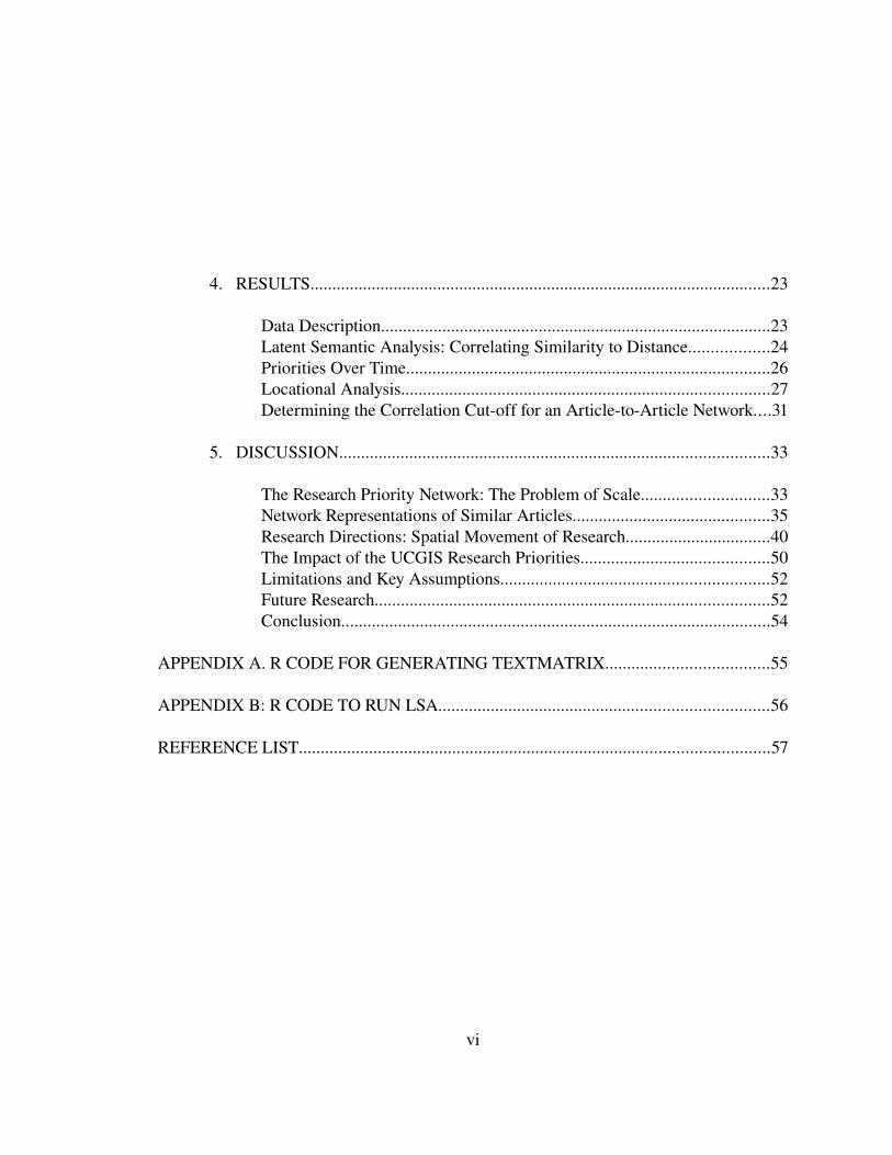
4.   RESULTS.........................................................................................................23

Data Description.........................................................................................23Latent Semantic Analysis: Correlating Similarity to Distance..................24Priorities Over Time...................................................................................26Locational Analysis....................................................................................27Determining the Correlation Cut­off for an Article­to­Article Network....31

5.   DISCUSSION..................................................................................................33

The Research Priority Network: The Problem of Scale.............................33Network Representations of Similar Articles.............................................35Research Directions: Spatial Movement of Research.................................40The Impact of the UCGIS Research Priorities...........................................50Limitations and Key Assumptions.............................................................52Future Research..........................................................................................52Conclusion..................................................................................................54

APPENDIX A. R CODE FOR GENERATING TEXTMATRIX.....................................55

APPENDIX B: R CODE TO RUN LSA...........................................................................56

REFERENCE LIST...........................................................................................................57

vi

LIST OF TABLES

Table      Page

1. UCGIS Research Priorities (first year of publication).....................................................3

2. UCGIS Research Priorities (with primary keywords)....................................................18

3. Secondary keyword­stems Derived with a .5 or greater Pearson Correlation to Primary Keyword "mobil­.".............................................................................................................19

4. Variations of Input Matrices for semantic analysis........................................................20

5. Summary count of data types.........................................................................................23

6. Number of articles published in each journal................................................................23

7. Research quantified: results from LSA of the year­by­year research priorities as a percentage of that year's research.......................................................................................27

8. The Ten Highest Correlated Locations Per Research Theme........................................30

9. Network Statistics for Correlation Cut­off Targets........................................................32

10.  Author key for Figure 10.............................................................................................38

11. Similarity between articles. Numbers in Italics are below the .8 cut­off......................41

12. Description of related networked articles....................................................................44

13. Location key for Figure 13...........................................................................................46

vii

LIST OF FIGURES

Figure      Page

1. An Example Latent Semantic Analysis Calculation.......................................................17

2. Articles Published as Year.............................................................................................23

3. Scatterplot of Article Similarity (correlation) vs. Distance (km)..................................24

4. Article Similarity (Grouped) vs. Distance (1,000 km)...................................................25

5. Papers Published at North American Research Locations, 1997­2007..........................28

6. Papers Published at European Research Locations, 1997­2007.....................................29

7. The knowledge domain network of the UCGIS priorities..............................................33

8. Different meanings of the word "scale."........................................................................35

9. Network representation of similarity index between GIS articles, 1997­2007...............35

10. Network representation of authors with highly­similar publications, 1997­2007. ......37

11. Map of one network of related articles.........................................................................42

12. Network representation of some related articles..........................................................43

13. Network representation of highly­correlated locations, 1997­2007.............................45

14. Information routes of highly­correlated articles...........................................................49

15. Route map of information flows of three or more articles...........................................50

16.  Percent Change in research themes, 1997­2007...........................................................51

viii

ABSTRACT

INNOVATION DIFFUSION IN GEOGRAPHIC INFORMATION RESEARCH

by

David A. Parr, B.S.

Texas State University­San Marcos

June 2008

SUPERVISING PROFESSOR: YONGMEI LU

Geographic Information Science (GIS) researchers analyze digital data to identify 

spatial patterns quantitatively. Following a similar approach, this thesis research reveals 

the diffusion dynamics of GIS research through analyzing the field's publications. A total 

of 985 GIS journal articles published between 1997 and 2007 in six different academic 

journals were examined. By assuming that each article was conducted at the institution 

listed as the primary author's affiliation, each journal article is evaluated using latent 

semantic analysis to reveal a set of correlations between the research themes of the 

articles year­by­year and location­by­location. With knowledge of the location and time of 

each publication, we show the spatial and thematic evolution of research activities in GIS.

ix

CHAPTER 1

INTRODUCTION

Geographic Information Science (GIS) has a brief yet fruitful history. Geographic 

information science emerged in the past four decades as a growing field that affects 

communication, travel, transport, location services, mobile services, and other aspects of 

the economic, commercial, and academic activities. In this paper, we consider the 

thematic changes in GIS research over eleven years from an innovation diffusion point of 

view. Innovation diffusion research studies how ideas  propagate through a society. 

This thesis research uses latent semantic analysis (LSA) to measure the research 

changes in GIS from 1997 to 2007. LSA begins with the full text of research articles and 

quantifies the similarity of these articles. The result is a similarity index, a value from ­1 

to 1, of the similarity for  each pair of articles. By grouping the articles according to 

author, author's affiliation location, year, or journal, LSA will quantify a similarity index 

among authors, locations, years, or journals. We also group articles by subject keywords 

in GIS to quantify the changes in research subjects over this eleven year period.

1

2

UCGIS Research Priorities

The University Consortium of Geographic Information Science (UCGIS) formed 

in 1988 and has grown to include 67 academic institutional members, four representative 

professional organizations and ten government/non­profit/industry organizations (Eames, 

2005). The organization has three purposes:

"To serve as an effective, unified voice for the geographic information 

science research community;

To foster multidisciplinary research and education;

To promote the informed and responsible use of geographic information 

science and geographic analysis for the benefit of society." 

(UCGIS, 2003, page 2)

In 1996, UCGIS published their first set of white papers on research priorities for 

geographic information science (UCGIS, 1996). Since then, updates were published in 

1998, 1999, 2000, 2002, and 2006. The consortium is a collaborative group of academic 

institutions, governmental organizations, and commercial GIS developers. In addition to 

recommending policy and legislation and setting goals for GIS education, the UCGIS 

advocates the advances in GIS research that are most important to its members. Listed in 

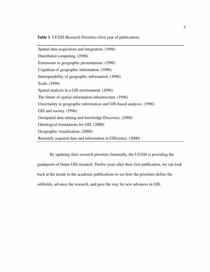
Table 1 are the research priorities (UCGIS, 1996; UCGIS, 2000).

3

Table 1. UCGIS Research Priorities (first year of publication).

Spatial data acquisition and integration. (1996)

Distributed computing. (1996)

Extensions to geographic presentations. (1996)

Cognition of geographic information. (1996)

Interoperability of geographic information. (1996)

Scale. (1996)

Spatial analysis in a GIS environment. (1996)

The future of spatial information infrastructure. (1996)

Uncertainty in geographic information and GIS­based analyses. (1996)

GIS and society. (1996)

Geospatial data mining and knowledge Discovery. (2000)

Ontological foundations for GIS. (2000)

Geographic visualization. (2000)

Remotely acquired data and information in GIScience. (2000)

By updating their research priorities biennially, the UCGIS is providing the 

guideposts of future GIS research. Twelve years after their first publication, we can look 

back at the trends in the academic publications to see how the priorities define the 

subfields, advance the research, and pave the way for new advances in GIS. 

CHAPTER 2

LITERATURE REVIEW

History of Innovation Diffusion Research

Innovation diffusion is a multi­disciplinary research area that traces its roots to 

early twentieth century scientists in sociology and anthropology. Gabriel Tarde, a French 

lawyer and judge writing The Laws of Imitation in 1903, identified the adoption or 

rejection of an innovation as a crucial variable in analysis. At the same time, the 

sociologist Georg Simmel (active years: 1890­1918) in Berlin developed a key idea for 

diffusion research: that groups of individuals could act as a set of coordinates of 

affiliations. By using individuals as the key structural element, Simmel anticipated 

aspects of later social network research sixty years before it became formalized in 

literature (Rogers, 2003).

The paper, “The Diffusion of Hybrid Seed Corn in Two Iowa Communities” 

(Ryan and Gross, 1943), was the first to use sociometric data to determine the rate and 

causes of innovation diffusion (Rogers, 2003). Dr. Bryce Ryan and Neal C. Gross 

interviewed 345 farmers in two communities using surveys to find when and why they 

had chosen to use hybrid corn. During the interviews, they also noted from whom the 

farmer received the hybrid corn. By statistically analyzing when and from whom each 

4

5

farmer began adopting the new corn seed, Ryan and Gross showed the difference between 

when a farmer first heard about hybrid corn and when they adopted it (Ryan and Gross, 

1943).

Ryan and Gross introduced several key principles of innovation diffusion. The 

channels of new information is often more important than the idea itself. Most farmers 

already knew about hybrid corn from salesmen, yet waited until several key early adopters 

tried the corn before adopting themselves. “The spread of knowledge and the spread of 

'conviction' are, analytically at least, two distinct processes” (Ryan and Gross, 1943, page 

21). They found that the rate of adoption over time was similar to the normal curve, where 

a slow acceptance by a few early adopters (also labeled 'opinion leaders') would be 

followed by the early majority of farmers, the late majority, and then the laggards who 

arrive last. This graph later became known as the S­Shaped Adoption Curve (Hägerstrand, 

1953; Rogers, 2003), a theory in Innovation Diffusion that predicts the rate of acceptance 

based on character types of the individual. Quantitatively, they were able to show that 

diffusion itself is a social process that occurs over time. Using this methodology, Ryan 

and Gross developed the framework that led to innovation diffusion as a field of research. 

Rural sociology was quick to adopt the innovation diffusion paradigm presented 

by Ryan and Gross, partly because technological innovation was seen as a key to 

successful development (Rogers, 2003). Since then, diffusion research has been included 

in the fields of economics, sociology, marketing, communications, management science, 

and not least of which, geography.

6

Innovation Diffusion as a Spatial Process

Torsten Hägerstrand, working at the University of Lund in Sweden, broke new 

ground with his 1953 thesis, Innovations förloppet ur korologisk synpunkt, translated as 

Innovation diffusion as a spatial process by Allan Pred in 1967.  Hägerstand was a 

geographer and therefore disposed to view diffusion as a spatial and temporal process. 

For his thesis, he studied the diffusion of the telephone, the automobile, and tuberculosis 

inoculations in the province of Östergotland in the 1920's, 1930's, and 1940's. Gathering 

data on soil conditions, population density, in­ and out­migrations to the region, farming 

conditions, the road network, and money transfers, Hägerstrand was able to model in 

detail the effects that these indicators played on influencing innovation adoption 

(Hägerstrand, 1953). 

Hägerstrand produced mathematical models using a Monte Carlo simulation to 

show which factors influenced diffusion using the laws of probability. A person's decision 

if and when to adopt an innovation is called the innovation decision process (Rogers, 

2003). Hägerstrand's model includes resistance, or the factors that impede adoption. 

Modeling in both time and space, Hägerstrand produced a time­series of maps that 

expected the diffusion field based on the spread from central locations, similar to Walter 

Christaller's Central Place Theory. Central Place Theory in innovation diffusion posits 

that innovations are first adopted in core places (such as large cities, and then move 

outwards to rural areas (Hägerstrand, 1952; Rogers, 2003). In his theory, Hägerstrand 

7

could show geographically how the innovation would diffuse in the region depending on 

the variables present in the population, the location, and the innovation.

Further papers expanded on Hagerstrand's model to arrive at a formulaic 

description of the process of innovation diffusion at a group or regional level (Strang and 

Tuma, 1993). The unit of analysis in diffusion studies had, from the onset, been at the 

group or regional level. Everett M. Rogers suggests in Diffusion of Innovations that the 

unit of analysis should instead be the individual (Rogers, 2003). An individual's decision 

may depend on their social connections or other, external types of communication. As the 

social peers adopt a change, the individual may reach a threshold, or point where they 

will themselves accept the innovation (Valente, 1996). The threshold model of innovation 

diffusion analysis is the precursor to the social network analysis that has followed.

Social Network Theory

A social network is a structure made of vertices of actors and interdependent 

linkages between them representing acquaintance. Actors are most often individuals, 

while the linkages can be various: exchanges of financial, informational, or technological 

means, markers of the spread of disease, and organizational structures, which can be both 

formal and informal groupings. Social networks are of interest because they represent the 

pattern of human interaction present in a social structure (Newman, 2000). The structure 

itself is of particular interest because it has implications for the spread of disease or 

information. 

8

Social network experiments began in the 1960's (Newman, 2000). Stanley 

Milgram examined small world social networks where typical distances are comparable 

with those on a random graph (Watts and Strogatz, 1998). In his experiment, Milgram 

sent an misaddressed letter meant for a stockbroker in Boston to a person in Nebraska 

who was chosen at random (Travers and Milgram, 1969). The average number of steps for 

the letter to arrive from the first person to final recipient was six, leading to the phrase 

“six degrees of separation,” or the network distance between any two ends of the human 

community.

Co-Citation and Co-authorship Networks

Citations were first used in the late 19th century by legal scholars (Kessler, 1963). 

In the early 1960's, Eugene Garfield and the Institute for Scientific Information began 

publishing the Scientific Citation Index (or, SCI), an index of paper­to­paper citations. A 

similar topic, bibliographic coupling, where one measures the amount that different 

papers cite the same sources, originated in 1963 (Kessler, 1963). The initial work drew 

few conclusions, but did present a methodology that would later be expanded (Small, 

1973; Small, 2003). White and Griffith created the first co­citation map (White and 

Griffith, 1981).

The emphasis of co­citation analysis is to determine the subject similarity and 

association of key ideas in a field, also known as the specialty structure of science (Small, 

1973.) A further relationship is established in the social structure of science, which can be 

9

determined by the co­authorship linkages in a science authorship network. An authorship 

network is a social network where vertices are authors and linkages are co­authorship 

status on one or more journal articles.

Co­authorship networks can be interpreted as structural representations of the 

collaborative nature of scientific research. The network structure of scientific 

collaborations has become an interest of great study, in part, because the data are easily 

available and complete. Several online databases, including MEDLINE (for biological 

research), NCSTRL (for computer science), and the Los Alamos e­Print Archive (for 

Physics), present large, easily accessible data sources for network researchers (Newman, 

2000). Most importantly, the nature of the edges (connections) are clearly defined 

(Newman, 2000; Newman, 2001). This ensures a reliability in the structure and validates 

the connection.

The clustering coefficient is a measure of the local connectedness within a small 

part of a network. It is defined as “the average fraction of pairs that of a person's 

collaborators who have also collaborated with each other” (Strogatz and Watts, 1998, p. 

441).  The clustering coefficient, as a measure of local connectedness in a large network, 

is only a measure of local activity and does not define the boundaries of a locality. 

Discovering community groups in networks has become a key research area in recent 

years (Chen, 2005; Newman, 2006).  The detection and definition of community 

structures, which are tightly connected subgroups with loose connections to the main 

network, is key to defining subgroups within the larger network of scientific 

10

collaborations. 

Newman (2006) expands on the community finding problem by choosing 

communities based on probabilities. His method, modularity, is defined as the number of 

edges in a group minus the expected number in an equivalent random group (Newman, 

2006). Using the eigenvalue and eigenvector for a modularity matrix generated from a 

network, each subnetwork can be iteratively checked for a positive modularity value. A 

positive value indicates that the subnetwork contribute to the total modularity; a zero or 

negative value indicates that the search can be stopped, as the subnetwork is not divisible 

further (Newman, 2006).

Newman has produced several studies based on co­authorship network analysis. 

One, entitled “Who is the best connected scientist?” (Newman, 2000), looks at the 

popular Erdös number phenomena. Paul Erdös was a Hungarian mathematician and 

frequent collaborator who produced over a thousand publications within his lifetime. 

Authors may assign an Erdös Number based on the shortest network distance away from 

Erdös in a co­authorship network. Therefore, persons who have coauthored a paper with 

Erdös have an Erdös number of one. Authors who have collaborated with an author who 

has an Erdös number of one would have a number of two, and so on.

Knowledge Domain Visualization and Latent Semantic Analysis

Research in the field of information visualization has also approached the issues 

of innovation and knowledge diffusion, as well as citation analysis. Knowledge domain 

11

visualization (often shortened as “KDViz”)  is the study of the dynamic, self­organized, 

and emergent complex intellectual system that underlies an emergent science (Chen, 

2006). There are three key procedures in producing a visualization: extracting the salient 

structures from a set of data, detecting abrupt changes and emerging trends, and creating 

a visualization to coherently represent a set of complex information.

Latent semantic analysis (LSA, also known as LSI, latent semantic indexing) 

computes the singular value decomposition matrices of a matrix showing the number of 

occurrences of a keyword or phrase in columns by the sources (books, journal articles, 

etc) in the rows. A binary function (0 or 1) can be substituted for the number of 

occurrences if only the appearance of a keyword or phrase in a work is considered. 

Singular value decomposition (or SVD) is a technique in matrix computations that 

decomposes a matrix into three orthogonal matrices, one of which will be a truncated 

singular value matrix containing the factors that explain the variance across the rows 

(Golub and Van Loan, 1996). 

Related pairings of articles or terms can be determined even when exact words or 

phrases do not match (Deerwester, Dumais, Furnas, Landauer, and Harshman, 1990). By 

representing the SVD results geographically in an n­dimensional space, the dot­product 

of two vectors represents their similarity. A network can then be built based on the 

measurement of similarities, which can then be used to visually represent the connections 

among journal articles.

Chen (1999; 2006) has provided examples of how co­citation analysis and 

12

document similarity can be used to create detail­rich models of knowledge domains. His 

work examines the Invisible Colleges, or scientists in a specialty group that may 

collaborate outside of normal geographic bounds. He digested the SCI (Scientific Citation 

Index) to find journal articles related to string theory in particle physics. Finding over 

150,000 articles, he selected only those that had been cited 35 or more times. The 

resulting documents were weighted based on time, since more recent documents may not 

had as long as a time to become cited as older documents. A Pathfinder analysis was 

performed on the data to remove unimportant links. A network diagram was color­coded 

to pinpoint turning points in scientific research and visualized the knowledge 

relationships in the field of particle physics (Chen, 1999).

CHAPTER 3

METHODOLOGY

Summary of Major Steps

● Collected journal articles from GIS journal websites, including full text, author 

names and author affiliations.

● Parsed data using small programs to collect names, dates (by year), place names, 

country, and affiliations from files and place them into a database.

● Verified names, affiliations for completeness and accuracy against the files and in 

the database.

● Ran initial latent semantic analysis to find secondary keywords highly correlated 

to the primary keywords derived from the UCGIS research themes.

● Created thirty­five textmatrices from articles, including matrices by author, 

location, country, article, year, journal, and place, and using full words, stemmed 

words, UCGIS keywords, weighted UCGIS keywords, and binary (1 or 0) word 

counts.

● Ran latent semantic analysis on each of the thirty­five textmatrices to generate 

correlated output matrices.

● Geocoded affiliation locations and calculate Euclidian distances between each 

13

14

location point to every other location.

● Ran correlation analysis between the distances and the semantic relationship 

values for each paired publications.

● Arranged articles in time­order to find important “topic burst” points.

● Produced an aggregate map for each GIS research theme showing the ten highest 

correlated research sites.

Data Collection, Processing, and Verification

The complete text of articles from the journals Transactions in GIS, International  

Journal of Geographic Information Science, Cartography and Geographic Information 

Science, GeoInformatica, and related GIS papers that appear in the Annals of the 

Association of American Geographers and the Professional Geographer constitute the 

sources of data. In total, there are 985 articles from the year 1997 to 2007. Also contained 

are the date of publication, the names of the authors and their affiliations at the time of 

the writing. Files were saved as PDF (portable document format) files and then converted 

to text.

Author affiliations, article titles, and date of publication were entered into a 

database using several small programs to check for completeness and accuracy. Checking 

accuracy begins by alphabetizing the list of author names and affiliations. Common 

discrepancies are capitalization choices in names, missing a middle initial, small 

differences in the naming of university departments, and the choice of complete names 

15

versus abbreviated named or nick­names. This can happen when one author appears under 

multiple names (“A. Smith”, “Alan Smith”, “Alan J. Smith”). Authors may have multiple 

affiliations in multiple locations. Affiliation to a given university does not guarantee that 

the author works only at one place. The common practice in research is to assign the first 

author status to the author that contributes the most substantial material to an article. 

While this is not always the case, there is no method known to divide article authorship 

appropriately. In all cases, the first address of the first author given in a paper was 

considered their affiliation location. 

Articles require unique identifiers for analytical work and reference in this paper. 

We use a standard format accepted in bibliographic research. Articles are identified as 

"XY2000" or "XY2000_JOURNAL", where "X" is the primary author's first name initial, 

"Y" is the primary author's last name initial, "2000" is the year of publication, and 

"JOURNAL" is a shortened form of the journal name that published the article. The 

article "Error Propagation Modeling in Raster GIS: Adding and Ratioing Operations" by 

Giuseppe Ariba, Daniel Griffith, and Robert Haining and published in 1999 in 

Cartography and Geographic Information Systems would therefore be identified as 

"GA1999" or "GA1999_CAGIS."

Geocoding

To  derive geographic distance between author affiliation locations, the addresses 

of these institutions must be geocoded. Geocoding is the process of converting an address 

16

into geographical coordinates, usually done via a dictionary lookup of toponyms, or place 

names, to a set of coordinates. Tatsuhiko Miyagawa contributed a perl module1 that uses 

Google Maps lookups to return geocoding data for a toponym. Addresses that do not 

return a set of coordinates are verified manually. To verify accuracy, all of the results 

were checked manually.

Latent Semantic Analysis

The programming language R has a latent semantic analysis module written by 

Fidolin Wild2, which we used to run analysis3. For an example of LSA code, see 

Appendix B: R code to Run Latent Semantic Analysis. The input for latent semantic 

analysis is a matrix of article names as row headers and word counts as column headers 

(Deerwester et al, 1990).  After creating a matrix of journal articles to words, a singular 

value decomposition (SVD) is performed to create three matrices: X = T0 . S0 . D0', where 

T0 and D0 have orthogonal columns, and S0 is a diagonal matrix of r x r, where r is the 

rank of X. For a graphical example, see Figure 1.

The next step is to compute an approximate matrix   that is generated from theχ  

largest k values of S0, T0, and D0' into T, S, and D'. This matrix    contains theχ  

independent associational structures in the matrix with the  noise removed. The SVD can 

be interpreted geometrically in the same manner as principle component analysis. The 

result of the SVD is a k­dimensional vector representing the location of each keyword and 

1 http://www.cpan.org/modules/by­module/Geo/Geo­Coder­Google­0.03.readme   ; accessed Saturday, February 9, 2008.

2 http://cran.r­project.org/src/contrib/Descriptions/lsa.html   ; accessed Tuesday, January 29, 2008.3 http://www.r­project.org   ; accessed Tuesday, January 29, 2008.

17

journal article. In this space, the cosine or dot product between vectors corresponds to 

their estimated similarity. 

Choosing UCGIS Thematic Keywords

To derive relationships among research themes, we must first choose keywords 

from the University Consortium of Geographic Information Science (UCGIS) research 

priorities. For each priority listed in Table 2, we identify one or two keywords to act as 

the primary search criteria. We do not need to find every exact, semantically­related term 

as each keyword is stemmed to a root word. Using stemming allows LSA to find plurals 

Figure 1. An Example Latent Semantic Analysis Calculation.

18

and alternate word forms of the keyword. The second step, below, ensures that alternate 

semantically­related terms are found and weighted.

Table 2. UCGIS Research Priorities (with primary keywords).

Spatial data acquisition and integration. (acquisition, integration)

Distributed computing. (distributed)

Extensions to geographic presentations. (representations)

Cognition of geographic information. (cognition)

Interoperability of geographic information. (interoperability)

Scale. (scale)

Spatial analysis in a GIS environment. (analysis)

The future of spatial information infrastructure. (infrastructure)

Uncertainty in geographic information and GIS­based analyses. (uncertainty)

GIS and society. (society)

Geospatial data mining and knowledge Discovery. (mining)

Ontological foundations for GIS. (ontological)

Geographic visualization. (visualization)

Remotely acquired data and information in GIScience. (remote)

A second group of highly­correlated keywords related to the primary keywords are 

found and weighted by their Pearson correlation. After generating an initial latent 

semantic index of articles to stemmed words, we run Pearson product­moment 

correlations on each column­by­column, which contain the stemmed words of all articles. 

These provide a similarity index between each stemmed word. In Table 3, we have listed 

the word­stems that are most highly correlated to the word­stem "mobil­," used here to 

connote the word "mobile."

19

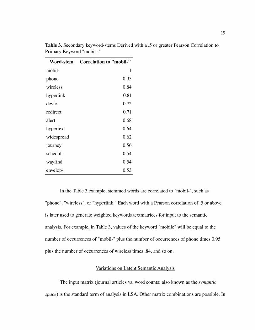
Table 3. Secondary keyword­stems Derived with a .5 or greater Pearson Correlation to Primary Keyword "mobil­."

Word­stem Correlation to "mobil­"

mobil­ 1

phone 0.95

wireless 0.84

hyperlink 0.81

devic­ 0.72

redirect 0.71

alert 0.68

hypertext 0.64

widespread 0.62

journey 0.56

schedul­ 0.54

wayfind 0.54

envelop­ 0.53

In the Table 3 example, stemmed words are correlated to "mobil­", such as 

"phone", "wireless", or "hyperlink." Each word with a Pearson correlation of .5 or above 

is later used to generate weighted keywords textmatrices for input to the semantic 

analysis. For example, in Table 3, values of the keyword "mobile" will be equal to the 

number of occurrences of "mobil­" plus the number of occurrences of phone times 0.95 

plus the number of occurrences of wireless times .84, and so on.

Variations on Latent Semantic Analysis

The input matrix (journal articles vs. word counts; also known as the semantic  

space) is the standard term of analysis in LSA. Other matrix combinations are possible. In 

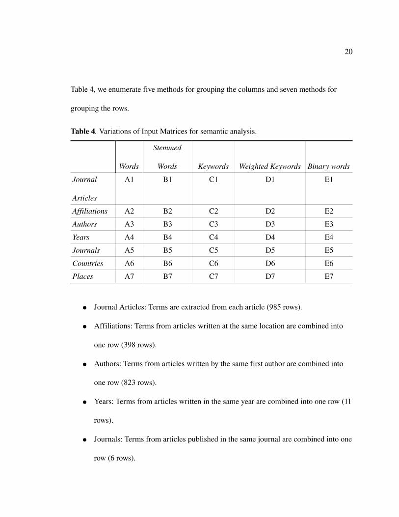
20

Table 4, we enumerate five methods for grouping the columns and seven methods for 

grouping the rows. 

Table 4. Variations of Input Matrices for semantic analysis.

Words

Stemmed 

Words Keywords Weighted Keywords Binary words

Journal 

Articles

A1 B1 C1 D1 E1

Affiliations A2 B2 C2 D2 E2

Authors A3 B3 C3 D3 E3

Years A4 B4 C4 D4 E4

Journals A5 B5 C5 D5 E5

Countries A6 B6 C6 D6 E6

Places A7 B7 C7 D7 E7

● Journal Articles: Terms are extracted from each article (985 rows).

● Affiliations: Terms from articles written at the same location are combined into 

one row (398 rows).

● Authors: Terms from articles written by the same first author are combined into 

one row (823 rows).

● Years: Terms from articles written in the same year are combined into one row (11 

rows).

● Journals: Terms from articles published in the same journal are combined into one 

row (6 rows).

21

● Countries: Term from articles with author locations in the same country are 

combined into one row (53 rows).

● Places: Terms from authors with the same university or professional affiliation are 

combined into one row (142 rows).

● Words: Word counts of words with five letters or more are used in the column­

space (50371 columns).

● Stemmed words: Words with the same root, including plurals and verb forms, are 

combined into one column (34290 columns).

● Keywords: Words with a correlation greater than .5 to the UCGIS subject 

keywords are combined into one column per keywords (16 columns total). See 

"Correlation."

● Weighted Keywords: Words correlated to the UCGIS subject keywords are 

combined using the weighted, correlated value to the keyword. (16 columns total).

● Binary words: Instead of a word count, either a 1 or 0 (found or not found) is 

placed in the column for each word (34290 columns).

In total, thirty­five latent semantic analyses produced 105 output matrices ­ three 

per LSA. But which analytical method is best for producing results? By using five 

different weighting techniques, we can run analysis of variance on the output to see which 

technique explains the most variability. Each set of LSA results is compared using an F­

test of variance.

22

Presentation

Representations can capture the results visually. The first, and simplest, is a scatter 

plot of similarity of journal articles (the results from the latent semantic analysis) to the 

distances. This is a quick way to show the relationship (if any) between distance and 

correlation. To show examples of data flow, a map will be created showing articles with 

high (over .8) similarity indices.

A network diagram is also used to visualize the relationships among articles. 

Nodes in this network represent articles, locations, authors, journals, dates, or subjects, 

and links indicate the inverse similarity index. More similar articles have smaller network 

distances. A network diagram illustrates with simple clarity the density, number, and 

connectivity of highly­similar articles.

CHAPTER 4

RESULTS

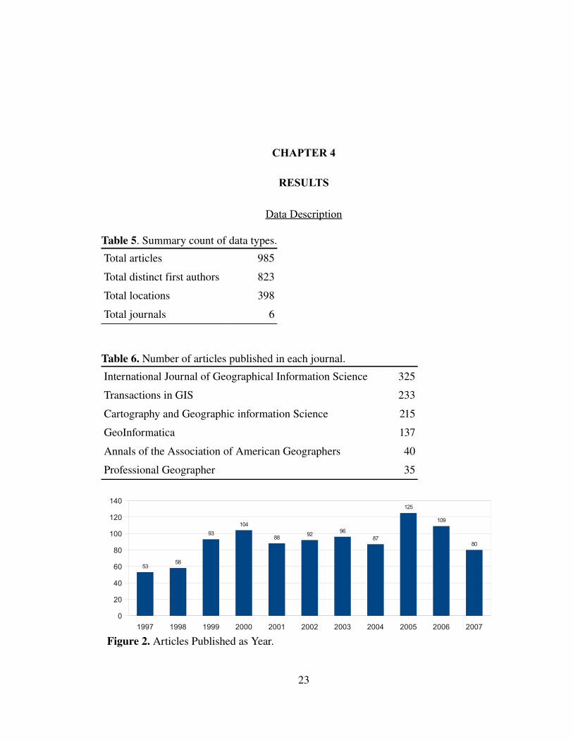
Data Description

Table 5. Summary count of data types.

Total articles 985

Total distinct first authors 823

Total locations 398

Total journals 6

Table 6. Number of articles published in each journal.

International Journal of Geographical Information Science 325

Transactions in GIS 233

Cartography and Geographic information Science 215

GeoInformatica 137

Annals of the Association of American Geographers 40

Professional Geographer 35

23

Figure 2. Articles Published as Year.1997 1998 1999 2000 2001 2002 2003 2004 2005 2006 2007

0

20

40

60

80

100

120

140

5358

93

104

8892

9687

125

109

80

24

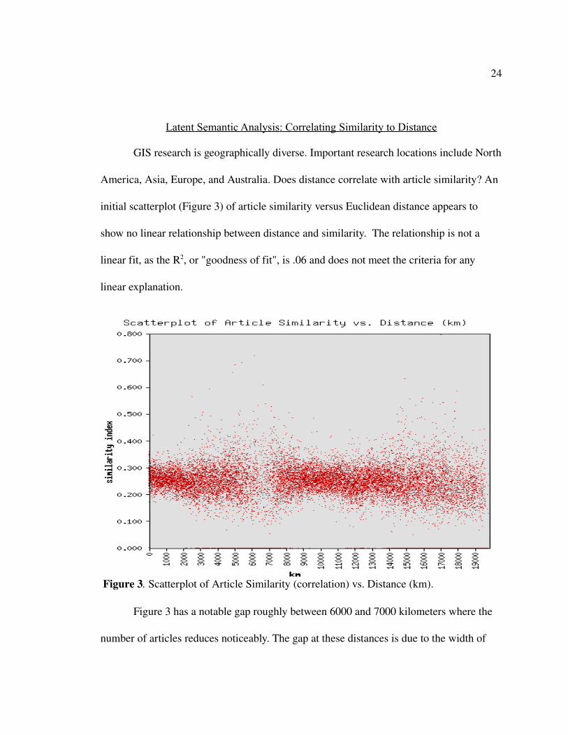
Latent Semantic Analysis: Correlating Similarity to Distance

GIS research is geographically diverse. Important research locations include North 

America, Asia, Europe, and Australia. Does distance correlate with article similarity? An 

initial scatterplot (Figure 3) of article similarity versus Euclidean distance appears to 

show no linear relationship between distance and similarity.  The relationship is not a 

linear fit, as the R2, or "goodness of fit", is .06 and does not meet the criteria for any 

linear explanation.

Figure 3 has a notable gap roughly between 6000 and 7000 kilometers where the 

number of articles reduces noticeably. The gap at these distances is due to the width of 

Figure 3. Scatterplot of Article Similarity (correlation) vs. Distance (km).

25

the Atlantic ocean. Distances larger than 7000 kilometers cross the Atlantic ocean, where 

distances less than 6000 kilometers are mostly intra­continental.  

In Figure 4, we show grouped similarity indices versus Euclidean distance. After 

grouping articles into similar ranges, there is a trend showing an inverse relationship 

between distance and similarity. Two articles are, on average, more similar the closer the 

authors' affiliation locations. Figure 4 includes a polynomial regression formula that 

accounts for 77% of the values (R2 = .77). In Chapter 5, we discuss some possible reasons 

for this relationship.

Figure 4. Article Similarity (Grouped) vs. Distance (1,000 km).

26

Priorities Over Time

With the original textmatrix substituted for a year­by­keyword matrix, we can 

quantify the year­by­year research results against the UCGIS research priorities after 

running latent semantic analysis (Table 7). From this, we can see several trends in GIS 

research. Some areas, such as modeling, representation, and acquisition, remain highly 

active from year­to­year. Research in infrastructure has become less active over time. 

Mobile computing research trends upward in the years 2006 and 2007. The values for 

scale are small compared to its value in geographic research. In Chapter 5, we discuss 

possible reasons why research in scale issues appears small.

27

Table 7. Research quantified: results from LSA of the year­by­year research priorities as a percentage of that year's research.

1997 1998 1999 2000 2001 2002 2003 2004 2005 2006 2007

modeling 23% 23% 23% 23% 23% 23% 23% 23% 24% 23% 23%

data mining .5% .5% .5% .5% .6% .5% .6% .6% .6% .5% .6%

ontology 3.0% 1.8% 5.3% 2.8% 6.6% 5.2% 7.0% 7.2% 8.6% 6.6% 8.1%

acquisition 6.7% 6.6% 7.0% 6.7% 7.2% 7.0% 7.2% 7.2% 7.4% 7.2% 7.4%

visualization 6.4% 5.8% 7.7% 6.3% 8.4% 7.6% 8.6% 8.7% 9.5% 8.4% 9.2%

representation  9.4% 9.4% 9.4% 9.4% 9.3% 9.4% 9.3% 9.3% 9.3% 9.3% 9.3%

society 11% 12% 9% 11% 7.5% 8.8% 7.2% 7.0% 5.7% 7.5% 6.1%

analysis 14% 14% 11% 14% 10% 12% 10% 9.9% 8.6% 10% 9.0%

infrastructure 3.0% 3.4% 2.2% 3.0% 1.8% 2.2% 1.7% 1.6% 1.1% 1.8% 1.3%

interoperability 1.5% 1.2% 1.9% 1.4% 2.2% 1.9% 2.2% 2.3% 2.5% 2.2% 2.5%

cognition 8.3% 8.7% 7.7% 8.4% 7.4% 7.7% 7.3% 7.2% 6.8% 7.4% 7.0%

mobile 1.6% 1.4% 2.0% 1.5% 2.3% 2.0% 2.3% 2.4% 2.7% 2.3% 2.6%

remote 3.6% 3.7% 3.4% 3.6% 3.3% 3.4% 3.3% 3.3% 3.1% 3.3% 3.2%

distributed 5.9% 6.1% 5.5% 6.0% 5.2% 5.5% 5.2% 5.1% 4.9% 5.2% 4.9%

scale .8% .8% .6% .8% .6% .7% .6% .6% .5% .6% .5%

uncertainty 2.3% 1.8% 3.5% 2.0% 4.2% 3.5% 4.3% 4.4% 5.1% 4.1% 4.9%

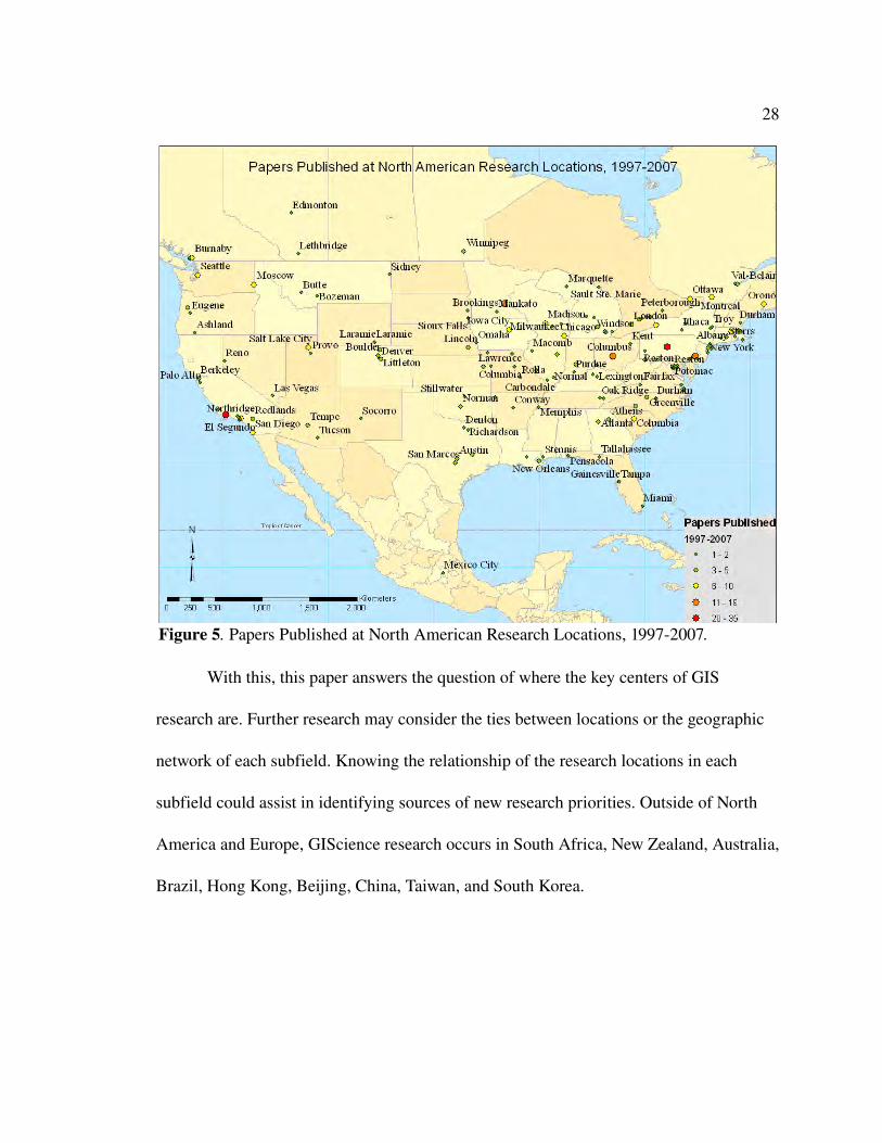
Locational Analysis

By modifying the original article­word textmatrix, we can create a location­word 

textmatrix and preform the latent semantic analysis as well. Doing so, we can find which 

locations have a high correlation with a particular research theme. It is possible that 

locations with a high correlation to a subject area would be key innovative sites for that 

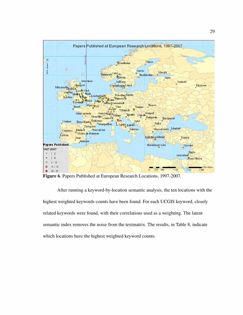
field. Figures 5 and 6 map primary research locations for some of the subject keywords.

28

With this, this paper answers the question of where the key centers of GIS 

research are. Further research may consider the ties between locations or the geographic 

network of each subfield. Knowing the relationship of the research locations in each 

subfield could assist in identifying sources of new research priorities. Outside of North 

America and Europe, GIScience research occurs in South Africa, New Zealand, Australia, 

Brazil, Hong Kong, Beijing, China, Taiwan, and South Korea.

Figure 5. Papers Published at North American Research Locations, 1997­2007.

29

After running a keyword­by­location semantic analysis, the ten locations with the 

highest weighted keywords counts have been found. For each UCGIS keyword, closely 

related keywords were found, with their correlations used as a weighting. The latent 

semantic index removes the noise from the textmatrix. The results, in Table 8, indicate 

which locations have the highest weighted keyword counts.

Figure 6. Papers Published at European Research Locations, 1997­2007.

30

Table 8. The Ten Highest Correlated Locations Per Research Theme.

Table 8 shows the ten highest correlated locations per research area between the 

years 1997­2007. Some locations appear multiple times: Santa Barbara, London, Hong 

Kong, and State College, Pennsylvania, all appear in ten or more of the lists. Some 

locations, such as Zurich (uncertainty) and Stuttgart (visualization), appear only once. 

Sheer quantity of publishing will affect these results. Hong Kong is a frequent publisher 

Cognition Data Mining Distributed Computing Spatial Data InfrastructureBurnaby, BC Beijing, China Canberra, Australia Columbus, OHColumbia, SC Burnaby, BC Edinburgh, UK Enschede, NetherlandsColumbus, OH Hong Kong, China Hong Kong, China Hong Kong, ChinaEnschede, Netherlands Ispra, Italy Leuven, Belgium Leeds, UKHong Kong, China London, UK London, UK London, UKLeeds, UK Madison, WI Madison, WI Melbourne, AustraliaMadison, WI Orono, ME Melbourne, Australia San Diego, CAMelbourne, Australia Santa Barbara, CA Orono, ME Santa Barbara, CAMunster, Germany State College, PA San Diego, CA Seattle, WAState College, PA Vienna, Austria Santa Barbara, CA State College, PA

Remote Computing Representation Scale GIS and SocietyCanberra, Australia Hong Kong, China Canberra, Australia Camden, NJEdinburgh, UK Ispra, Italy Edinburgh, UK Columbus, OHHong Kong, China Leeds, UK Enschede, Netherlands Enschede, NetherlandsLondon, UK London, UK Hong Kong, China London, UKMadison, WI Madison, WI London, UK Melbourne, AustraliaMelbourne, Australia Orono, ME Madison, WI Minneapolis, MNOrono, ME Richmond, BC Melbourne, Australia San Diego, CASanta Barbara, CA Santa Barbara, CA San Diego, CA Santa Barbara, CAState College, PA State College, PA Santa Barbara, CA Seattle, WAVienna, Austria Vienna, Austria State College, PA State College, PA

Interoperability Mobile Computing Uncertainty VisualizationBurnaby, BC Camden, NJ Canberra, Australia Columbia, SCEnschede, Netherlands Colubus, OH Edinburgh, UK Columbus, OHHong Kong, China Enschede, Netherlands Hong Kong, China Enschede, NetherlandsLeeds, UK London,UK Leuven, Belgium Hong Kong, ChinaLondon, UK Melbourne, Australia London, UK London, UKMelbourne, Australia Minneapolis, MN Orono, ME Madison, WIMunster, Germany San Diego, CA Richmond, BC Melbourne, AustraliaOrono, ME Santa Barbara, CA Santa Barbara, CA Santa Barbara, CASanta Barbara, CA Seattle, WA Vienna, Austria State College, PAState College, PA Southampton, UK Zurich, Switzerland Stuttgart, Germany

31

and appears often. Imprecise language will also impact how the relationship between 

location and theme is determined. LSA infers semantic context, but language is never 

exact. Words have multiple meanings and multiple words can share a single meaning. The 

"looseness" of language will add noise to the data and affect the quality of the results.

Determining the Correlation Cut-off for an Article-to-Article Network

Because language is not mathematically precise, the results of the semantic

analysis are all correlated to each other at some level. In order to make sense of the

relationships, some correlation cut-off is necessary. In Table 9, we show several potential

cut-offs for a correlation value. At .5, the network of related articles is dense and rich. On

the other end, .95 has no articles and .9 has a small network of only twenty.

For the purposes of this research, we choose .8 as a correlation to define highly-

correlated links between articles. We do not need every link, only the most salient. At .8,

the correlation links are both abundant and meaningful (see the "Network

Representations of Similar Articles" section in Chapter 5). At lower cut-offs, the network

is unwieldy to manage. A denser network would also require advanced network analysis

techniques to find community structures which denote meaning. For these reasons, .8 is

chosen as the correlation cut-off.

32

Table 9. Network Statistics for Correlation Cut­off Targets.

Correlation Cut­off

Vertices (out of % possible)

Edges (Network Density)

Network Structure

0.5 975 (99%) 34880 (4%)

0.6 886 (90%) 10046 (1%)

0.7 603 (61%) 2284 (.2%)

0.8 217 (22%) 402 (.04%)

0.9 20 (2%) 20 (<1%)

0.95 0 (0%) 0 (0%)

CHAPTER 5

DISCUSSION

The Research Priority Network: The Problem of Scale

33

Figure 7. The knowledge domain network of the UCGIS priorities.

34

In Chapter 4, we found the terms that were highly correlated with the UCGIS 

subject keywords.  To show how the subject keywords are related, we have correlated each 

keyword with each other keyword. In Figure 7, we link subjects that have a .8 Pearson 

correlation or higher. The network is a conceptual framework to demonstrate how the 

research priorities are thus related in the GIS knowledge domain.

Some areas of research are tightly coupled. Logically, "analysis" is linked to 

"visualization", "acquisition", "cognition", "distributed computing", "society", 

"uncertainty", "and "interoperability." "Representation" is linked to "visualization", 

"society", and "modeling." "Remote computing" is lined to "distributed computing."

"Scale", as a semantic subject, is loosely connected to the other terms and only 

directly connected to "data mining." At first, this appears counterintuitive. Many 

geographers would argue that scale is involved in many, if not all, types of geographical 

analysis. Scale has two particular characteristics that may explain its outsider status. If 

scale is, as theorized, involved in most geographic research, then the impact of the term 

"scale" may be deemed noise by the latent semantic algorithm. In a word frequency 

count, "scale" is the 53rd most frequently appearing term, excluding common words such 

as "the", "if", etc. Words that are universally pervasive will be considered noise by LSA.

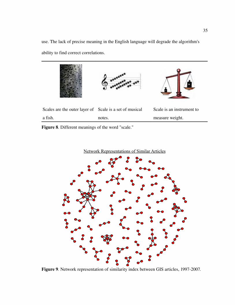
The imprecise meaning of "scale" may also impact these results. The term "scale" 

has many definitions: "scale" can mean a fractional geographic representation, a set of 

musical notes, an instrument to measure weight, or the outer layer of a reptile or fish (See 

Figure 8). Latent semantic analysis depends on the meaning and context of the words in 

35

use. The lack of precise meaning in the English language will degrade the algorithm's 

ability to find correct correlations.

Scales are the outer layer of 

a fish.

Scale is a set of musical 

notes.

Scale is an instrument to 

measure weight.

Figure 8. Different meanings of the word "scale."

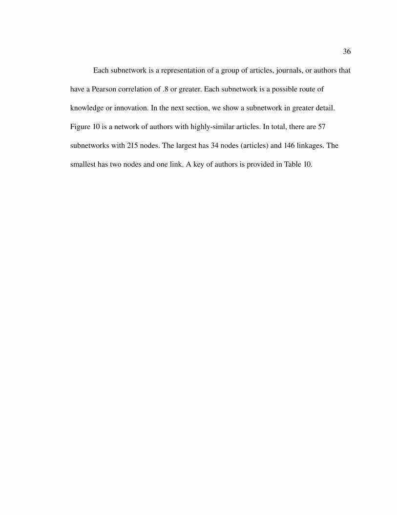
Network Representations of Similar Articles

Figure 9. Network representation of similarity index between GIS articles, 1997­2007.

36

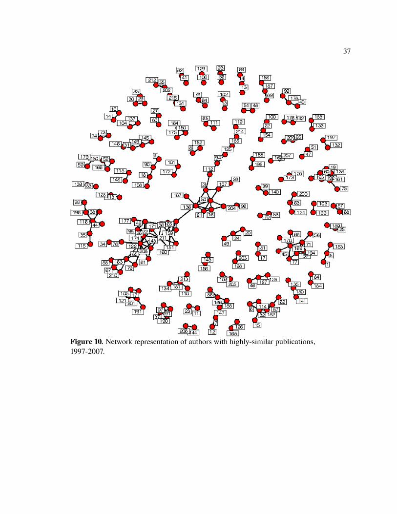
Each subnetwork is a representation of a group of articles, journals, or authors that 

have a Pearson correlation of .8 or greater. Each subnetwork is a possible route of 

knowledge or innovation. In the next section, we show a subnetwork in greater detail. 

Figure 10 is a network of authors with highly­similar articles. In total, there are 57 

subnetworks with 215 nodes. The largest has 34 nodes (articles) and 146 linkages. The 

smallest has two nodes and one link. A key of authors is provided in Table 10.

37

Figure 10. Network representation of authors with highly­similar publications, 1997­2007.

38

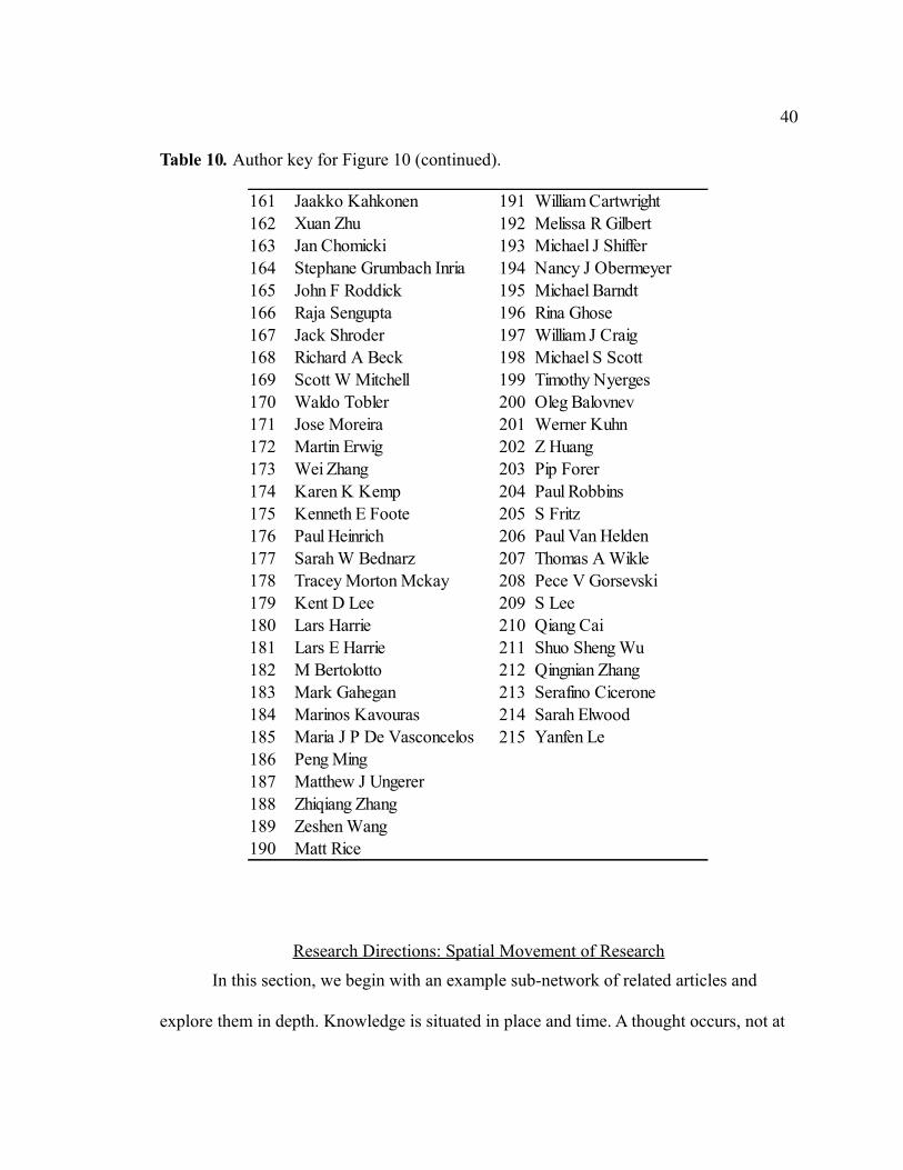
Table 10. Author key for Figure 10.

1 412 Jennifer Miller 42 Keven Roth3 43 Melissa Lamont4 445 Anthony G Cohn 45 Theodore Saunders6 467 478 489 4910 Antonio Corral 5011 51 Peter Fisher12 5213 Maria A Cobb 5314 Aileen Buckley 5415 5516 5617 5718 5819 5920 6021 Jessica Smith 6122 62 Fritz C Kessler23 George Taylor 6324 64 John Cloud25 65 Yang Cheng26 6627 Anthony C Robinson 6728 Terry A Slocum 6829 6930 7031 Barry Smith 7132 72 John Pickles33 7334 Christine E Dunn 74 David J Coleman35 Eric Sheppard 7536 7637 7738 78 Steve R Thorpe39 W H Erik De Man 79 William Duane40 80

Abhik Das Demin Xiong

Anna Oldak Sabine Grunwald Renee E Sieber

Sanjiang Li Boriana Deliiska Anton J J Van Rompaey P Agarwal D Karssenberg Bruce H Carlisle Michele Crosetto Howard Veregin

J Oksanen Jun Zhang Ashok Samal Byong Nam Choe

Olli Jaakkola Chaoqing Yu

Timothy Trainor Walter Collischonn Alan M Maceachren Charles Dietzel Menno Jan Kraak Claire A Jantz Alexey V Postnikov Qingfeng Guan Michael Heffernan Xiaojun Yang Allan Brimicombe Cengizhan Ipbuker

Diederik Van Leeuwen Allison Kealy

Ivan G Nestorov Annu Maaria Nivala Georg Gartner Karen Wealands Charles B Jackel

Matej Gombosi Ching Chien Chen

B Jiang Sagi Filin Bin Jiang Christian Kiehle

Rob Lemmens Margarita Kokla Barbara P Buttenfield Chuanrong Zhang

Z R Peng Ian Masser Claudio Paniconi Michael F Goodchild Puneet Srivastava R E Sieber

Bastiaan Van Loenen Claus Rinner

39

Table 10. Author key for Figure 10 (continued).

81 121 Eric Keys82 122 John Findley83 Kevin Hawley 12384 12485 Geoffrey Anderson 12586 Iain M Brown 12687 12788 Daniel G Brown 12889 12990 13091 13192 David Martin 13293 Nigel Walford 13394 13495 Lars Bernard 13596 13697 Marion Jones 13798 13899 139100 140 Hui Lin101 141102 142103 Dan Lin 143104 144105 145106 Danielle J Marceau 146107 Tamas Abraham 147108 Darla K Munroe 148109 149110 150111 151112 152113 153114 Dawn J Wright 154115 Denis J Dean 155116 156 Steve Jacoby117 157118 E A De Kemp 158119 159 J Lee120 Trevor Harris 160

Robert D Feick Cory L Eicher

Eva Klien Daniel Caldeweyher I Budak Arpinar

Florent Joerin Luis A Bojorquez Tapia

Lysandros Tsoulos Francois Lecordix Mahes Visvalingam

Martin Paegelow S Mustiere Daniel W Mckenney Frederico Fonseca Marcel Yri Fulong Wu

Xia Li Fang Ren

David Puliar Hongbo Yu Feras M Ziadat

Soohong Park J Gao Stefan Kienzle

Diansheng Guo Geoffrey Blewitt Vladimir Estivill Castro Gertraud Peinel Donggyu Park Leila De Floriani Georg Stadler Mahdi Abdelguerfi Steven Van Dijk

Steven Zoraster K Raptopoulou Tycho Strijk Victor Teixeira De Almeida Giuseppe Arbia

Wenzhong Shi Graeme Aggett Piotr Jankowski

J Crompvoets Gregory Vert James Boxall Harold Moellering John A Shuler Max J Egenhofer John Kelmelis Helen Couclelis Y Georgiadou Sara I Fabrikant

Robin G Fegeas Isaac Karikari

E Lynn Usery Jeong Chang Seong Wolfgang Hoeschele

Jason Dykes Kevin B Sprague

Jiyeong Lee

40

Table 10. Author key for Figure 10 (continued).

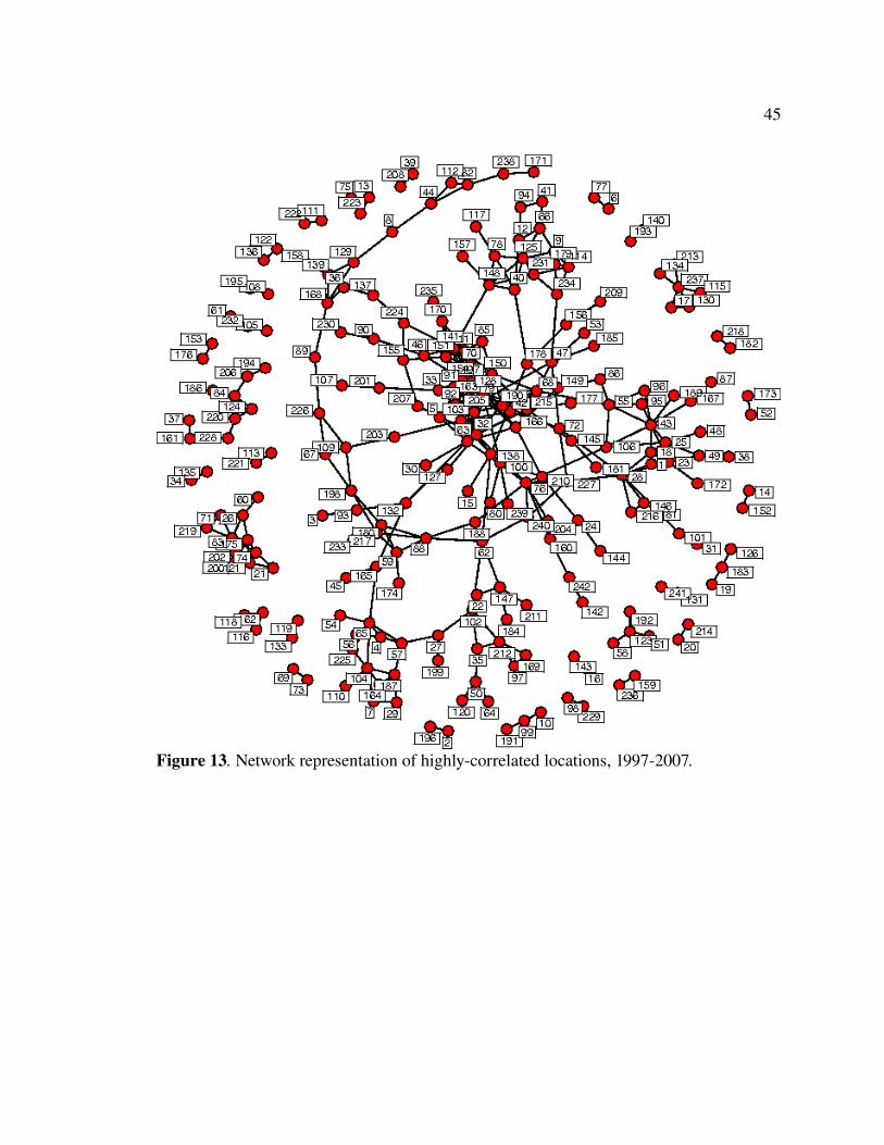
Research Directions: Spatial Movement of Research

In this section, we begin with an example sub-network of related articles and

explore them in depth. Knowledge is situated in place and time. A thought occurs, not at

161 191 William Cartwright162 192 Melissa R Gilbert163 193164 194165 195166 196167 197 William J Craig168 Richard A Beck 198 Michael S Scott169 Scott W Mitchell 199170 200171 201 Werner Kuhn172 202 Z Huang173 203174 Karen K Kemp 204 Paul Robbins175 Kenneth E Foote 205 S Fritz176 Paul Heinrich 206177 207178 208179 Kent D Lee 209 S Lee180 Lars Harrie 210181 Lars E Harrie 211182 212183 213184 214 Sarah Elwood185 215186187188189190 Matt Rice

Jaakko Kahkonen Xuan Zhu Jan Chomicki Michael J Shiffer Stephane Grumbach Inria Nancy J Obermeyer John F Roddick Michael Barndt Raja Sengupta Rina Ghose Jack Shroder

Timothy Nyerges Waldo Tobler Oleg Balovnev Jose Moreira Martin Erwig Wei Zhang Pip Forer

Paul Van Helden Sarah W Bednarz Thomas A Wikle Tracey Morton Mckay Pece V Gorsevski

Qiang Cai Shuo Sheng Wu

M Bertolotto Qingnian Zhang Mark Gahegan Serafino Cicerone Marinos Kavouras Maria J P De Vasconcelos Yanfen Le Peng Ming Matthew J Ungerer Zhiqiang Zhang Zeshen Wang

41

random in the ether, but in a person's mind while he is driving or she is chopping the

onions. Published research is transmitted through the internet, libraries, papers, meetings,

books, and journals.

Table 11. Similarity between articles. Numbers in Italics are below the .8 cut­off.

BC2005 GA1999 JO2006 PF1998 WS2003

BC2005 1.000 .738 .856 .832 .698

GA199 .738 1.000 .821 .840 .826

JO2006 .856 .821 1.000 .906 .780

PF1998 .832 0.84 .906 1.000 .813

WS2003 .698 .826 .780 .813 1.000

42

Figure 11. Map of one network of related articles.

43

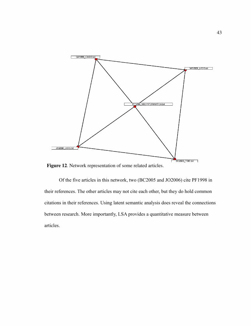
Of the five articles in this network, two (BC2005 and JO2006) cite PF1998 in

their references. The other articles may not cite each other, but they do hold common

citations in their references. Using latent semantic analysis does reveal the connections

between research. More importantly, LSA provides a quantitative measure between

articles.

Figure 12. Network representation of some related articles.

44

Table 12. Description of related networked articles.

BC2005 Title: Modeling the Spatial Distribution of DEM Error

Author: Bruce H. Carlisle (University of Northumbria)

Journal: Transactions in GIS, 2005

Location: Newcastle, UK

JO2006 Title: Uncovering the statistical and spatial characteristics of fine toposcale 

DEM error

Authors: J. Oksanen, T. Sarjakoski (Finnish Geodesic Institute)

Journal: IJGIS, 2006

Location: Masala, Finland

PF1998 Title: Improved Modeling of Elevation Error with Geostatistics

Author: Peter Fisher (University of Leicester)

Journal: GeoInformatica, 1998

Location: Leicester, UK

GA1999 Title: Error Propagation Modeling in Raster GIS: Adding and Ratioing 

Operations

Authors: Giuseppe Arbia, Daniel Griffith, Robert Haining

Journal: Cartography and GIS, 1999

Location: Pescara, Italy

WS2003 Title: Modeling error propagation in vector­based buffer analysis

Authors: Wenzhong Shi (Hong Kong Polytechnic), Chui Cheung, 

Changqing Zhu

Journal: IJGIS, 2003

Location: Hong Kong, China

45

Figure 13. Network representation of highly­correlated locations, 1997­2007.

46

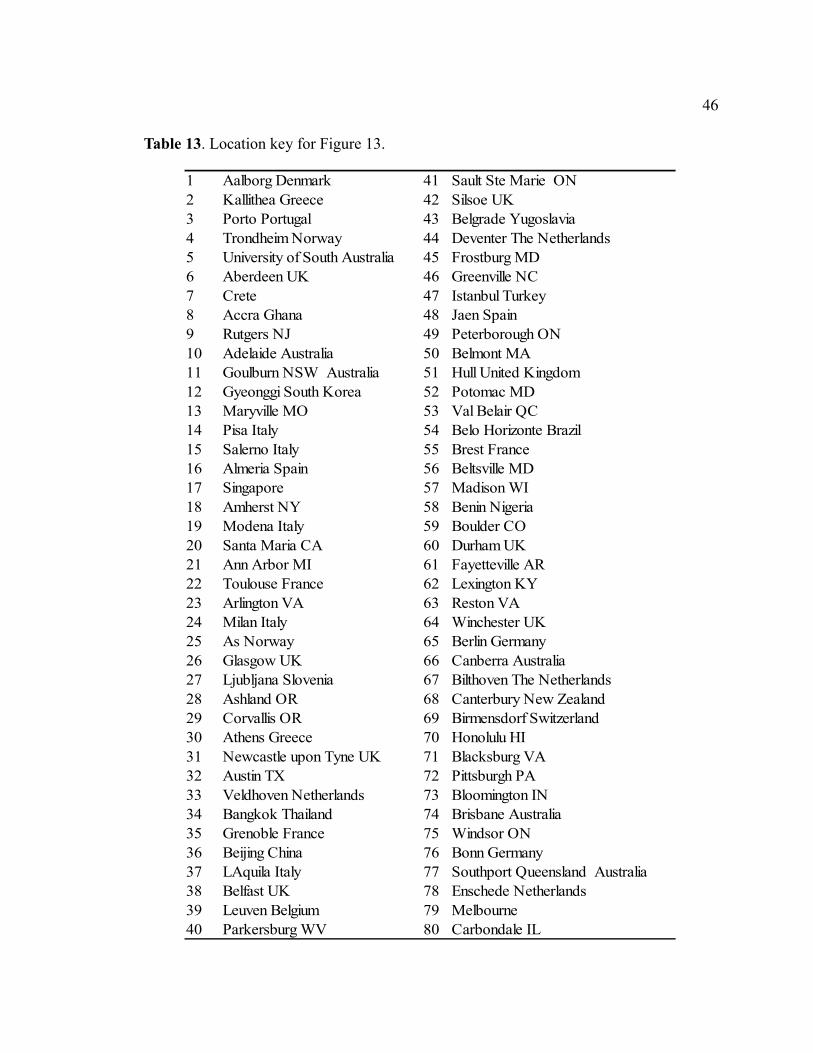
Table 13. Location key for Figure 13.

1 Aalborg Denmark 41 Sault Ste Marie ON2 Kallithea Greece 42 Silsoe UK3 Porto Portugal 43 Belgrade Yugoslavia4 Trondheim Norway 44 Deventer The Netherlands5 University of South Australia 45 Frostburg MD6 Aberdeen UK 46 Greenville NC7 Crete 47 Istanbul Turkey8 Accra Ghana 48 Jaen Spain9 Rutgers NJ 49 Peterborough ON10 Adelaide Australia 50 Belmont MA11 Goulburn NSW Australia 51 Hull United Kingdom12 Gyeonggi South Korea 52 Potomac MD13 Maryville MO 53 Val Belair QC14 Pisa Italy 54 Belo Horizonte Brazil15 Salerno Italy 55 Brest France16 Almeria Spain 56 Beltsville MD17 Singapore 57 Madison WI18 Amherst NY 58 Benin Nigeria19 Modena Italy 59 Boulder CO20 Santa Maria CA 60 Durham UK21 Ann Arbor MI 61 Fayetteville AR22 Toulouse France 62 Lexington KY23 Arlington VA 63 Reston VA24 Milan Italy 64 Winchester UK25 As Norway 65 Berlin Germany26 Glasgow UK 66 Canberra Australia27 Ljubljana Slovenia 67 Bilthoven The Netherlands28 Ashland OR 68 Canterbury New Zealand29 Corvallis OR 69 Birmensdorf Switzerland30 Athens Greece 70 Honolulu HI31 Newcastle upon Tyne UK 71 Blacksburg VA32 Austin TX 72 Pittsburgh PA33 Veldhoven Netherlands 73 Bloomington IN34 Bangkok Thailand 74 Brisbane Australia35 Grenoble France 75 Windsor ON36 Beijing China 76 Bonn Germany37 LAquila Italy 77 Southport Queensland Australia38 Belfast UK 78 Enschede Netherlands39 Leuven Belgium 79 Melbourne40 Parkersburg WV 80 Carbondale IL

47

Table 13. Location key for Figure 13 (continued).

81 Dunedin New Zealand 12182 122 Clayton Victoria Australia83 Lincoln New Zealand 12384 Muenster Germany 124 Cologne Germany85 Vancouver BC 125 Oslo Norway86 Bristol England 126 Conway AR87 Oak Ridge TN 12788 Research Triangle Park NC 128 Norwich UK89 Santa Barbara CA 129 Nottingham UK90 13091 Woods Hole MA 131 Fairfax VA92 132 Sheffield UK93 133 Washington DC94 134 Curitiba Brazil95 135 Richmond BC96 Butte MT 13697 Bucharest Romania 137 London ON98 East Lansing MI 138 Delft The Netherlands99 Wolverhampton UK 139 Fredericton NB100 140101 East Midlands Airport 141 Milwaukee WI102 142 Whitewater WI103 143 Dublin Ireland104 University of Ireland 144 Taipei Taiwan105 145106 Cambridge MA 146107 147 Newcastle UK108 Normal IL 148109 149 Portsmouth UK110 Iowa City IA 150 Sterling VA111 Kingston upon Thames UK 151 Edinburgh UK112 Tampa FL 152 Perth Australia113 153 El Segundo CA114 154 Haifa Israel115 Seattle WA 155 St Louis MO116 Champaign IL 156 Eugene OR117 Kent State University 157 Greensboro NC118 Lisbon Portugal 158 Fort Collins CO119 North Shore New Zealand 159120 Charlotte NC 160

Mankato MNLeicster UK

Zaragoza Spain

Huntingdon UK

Suitland MD Rolla MO

Brookings SDPresov SlovakiaStorrs CTBrookville NY

Darmstadt Germany

Cagliara Italy Karlsruhe Germany

Friedrichshafen GermanySao Paulo Brazil

Wernigerode Germany Ulm GermanyDusseldorf Germany

Nijimegen The NetherlandsKildare Ireland

Terra Haute IN

Casault QuebecCorvalis OR

Porto Alegre BrazilRoorkee India

48

Table 13. Location key for Figure 13 (continued).

161 Frankfort KY 202162 203 Leiden Netherlands163 Gainesville FL 204 Rockville MD164 University of Queensland 205165 Geneva Switzerland 206 University of Jordan166 Mexico City Mexico 207167 Split Croatia 208 Toronto ON168 209 London UK169 210 Tallahassee FL170 211 Ypsilanti MI171 212172 Gloucester Point VA 213173 214174 Mount Pleasant MI 215 Memphis TN175 Marquette MI 216176 Guangzhou China 217177 Southampton UK 218 Montevideo Uruguay178 Hagen Germany 219 Moscow ID179 220 Moscow Russia180 221 Winnipeg Manitoba181 222 New Delhi India182 223183 224 New Orleans LA184 225 Newark DE185 226186 Leeds UK 227187 Sofia Bulgaria 228 Newcastle NSW Australia188 Provo UT 229189 Horten Norway 230 Tucson AZ190 St Martin France 231 Orono ME191 Ithaca NY 232192 State College PA 233 Paris France193 Jerusalem Israel 234 Pensacola FL194 235 Pretoria South Africa195 236196 Kent OH 237197 238 Richardson TX198 University Park PA 239 Syracuse NY199 Knoxville TN 240 Salt Lake City UT200 Montreal QC 241 Yokohama Japan201 West Long Branch NJ 242

Masala FinlandKirksville MO

Lethbridge Canada

Louvain Belgium

Genova ItalyYangsan City South KoreaGlamorgan UKUniversity of Keele Macomb IL

Osijek CroatiaGrahamstown South Africa Maribor Slovenia

Stennis Space Center MSTelemark Norway

Le Chesnay FranceThessaloniki GreeceHannover GermanyKonya Turkey Wallingford UKPontypridd UKZurich SwitzerlandHeraklion Greece Pescara Italy

Otago New Zealand

Townsville Australia

enschede Netherlands

Stillwater OKKeele University Redlands CA

Wageningen NetherlandsSankt Augustin Germany

Trento Italy

49

Figure 14. Information routes of highly­correlated articles.

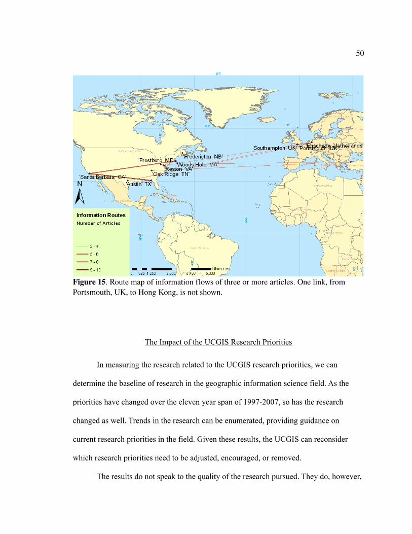
In Figure 14, we present a route map of information flows, as represented by 

similar articles and the connections between them. Some striking patterns emerge. 

Clearly, many connections exist between North American and European locations, both 

within and between these continents. Even more striking is that other locations, such as 

those in Brazil, South Africa, China, and New Zealand, are more closely related to North 

American and European locations then they are to closer locations. Only in one case, in 

Australia, does a link occurs with both nodes locally in that country outside of North 

America or Europe. 

These results may indicate a bias in language. As all of the publications are in 

English, this may limit information flows between countries of other native languages. 

Institutional funding and resources may also present challenges. North American and 

European institutions may be better funded or have more access to GIS literature. 

50

The Impact of the UCGIS Research Priorities

In measuring the research related to the UCGIS research priorities, we can

determine the baseline of research in the geographic information science field. As the

priorities have changed over the eleven year span of 1997-2007, so has the research

changed as well. Trends in the research can be enumerated, providing guidance on

current research priorities in the field. Given these results, the UCGIS can reconsider

which research priorities need to be adjusted, encouraged, or removed.

The results do not speak to the quality of the research pursued. They do, however,

Figure 15. Route map of information flows of three or more articles. One link, from Portsmouth, UK, to Hong Kong, is not shown.

51

provide the UCGIS with information on how research has changed, where different types

of research are being performed, and how the knowledge domain is structured internally.

A graph of percent change in GIS research themes from 1997 is presented in 

Figure 16. One theme, infrastructure, is less prevalent in 2007 than in 1997. Some themes, 

such as society and analysis, are virtually identical in the amount of research in 2007 as 

they were in 1997. Ontology and data mining have risen significantly as the themes were 

lightly considered at the beginning of the study. The "stacking effect," where trends 

appear to move in unison, is an artifact. GIS themes are not completely independent, thus 

related themes will move in concert.

Year

acquisitionanalysiscognitiondata_miningdistributedinfrastructureinteroperabilitymobilemodelingontologyremoterepresentationscalesocietyuncertaintyvisualization

Figure 16.  Percent Change in research themes, 1997­2007.

1997 1998 1999 2000 2001 2002 2003 2004 2005 2006 2007

-100

0

100

200

300

400

500

600

700

800

900

52

Limitations and Key Assumptions

Inherent in most innovation diffusion studies is a process known as the pro­

innovation bias (Rogers, 2003). Pro­innovation bias is the tendency to view only 

successful changes and adaptations in innovation and ignore failing ones. This study does 

not include unpublished or rejected manuscripts as these do not contribute to diffusion.

Because of cost restrictions, digital bibliographic data available to academic 

institutions is limited. Therefore, the data available were restricted to the years 1997 to 

2007. During this period, a more complete snapshot of journal articles were available. 

Prior to 1997, easily available digital copies of research were not available. Therefore, the 

study was limited exclusively from 1997 to 2007. In some cases, the full text of research 

papers within these years were not available. In all cases, book reviews, editorials, and 

other non­research papers were excluded.

Future Research

Semantic analysis provides a method to identify and quantify the relationship

among published research. While it may not speak to the quality of the research, it can

establish linkages between research, keywords, time, and space. This thesis has

demonstrated several methods of analyzing the research changes over time (from 1997 to

2007) and over space. The analysis has identified words closely related to the subject

keywords. Future research may explore how semantic alternatives are used in different

locations.

53

Previous academic research has focused on the citation network as the structure of

scientific connectivity (Small, 1973; White and Griffith, 1981; Newman, 2000; Newman,

2001). Citation networks are limited in that all citation values are binary: 1 for a work

that is cited, 0 for a work that is not cited. Not all citations can be assumed to be of equal

value, however. Latent semantic analysis could be used to find the similarity indices

between journal articles and other published scholarly research. A similarity index may

be a suitable replacement for the binary citation values.

Future research can expand on the networking analysis of latent semantic analysis

(LSA) results. Options include optimizing the correlation cut-off values, finding

community structure, or measuring the differences among multiple models of network

types.

LSA is based on singular value decomposition, which uses two dimensions of

analysis. Higher-order singular value decomposition (HOSVD) analyzes matrices in three

or higher dimensions. A higher-order LSA could explore multiple dimensions of analysis,

incorporating authorship, location, or other measures directly into the LSA. Doing so

would provide a method to remove noise from several dimensions at the same time.

Using thematic keywords in a higher-order LSA might remove some publication

frequency noise.

Each-correlated article pair represents a spatial connection as well as thematic.

The number of links between locations is an indicator of related research directions.

Comparison subjects may include airplane flight networks. We could demonstrate the

direction, and frequency of thematic connections between research locations on a map.

54

Conclusion

Latent semantic analysis has proven to be a valuable tool to indicate similar 

articles. In this report, we have shown that it can be used to establish relationships 

between locations, authors, journals, and years. Using weighted keywords, we can show 

directions in research over time. Each of these methods has implications for 

understanding the specialty structure of a science and how that structure changes over 

time.  

Researchers in GIScience are not isolated individuals, but rather a network of 

collaborators who work within organizations, departments, and professional groups to 

advance knowledge, cultivate relationships, and gain feedback on their work. Feedback on 

research is an integral part of the modern academic system; researchers are evaluated by 

peers, editors, and the public­at­large. Organizations such as the University Consortium 

of Geographic Information Science and the Association of American Geographers are 

catalysts that provide guidance and direction and foment these networks. This study 

suggests a methodology for quantifying and measuring what types of research are being 

produced where are by whom. Organizational networks should use these methods to 

establish directions of scientific research. 

APPENDIX A. R CODE FOR GENERATING TEXTMATRIX

The R code below creates a stemmed textmatrix from the directory

"ALL_ARTICLES." The minimum word length is four letters, and all words are

stemmed. The output is written into a comma separated values file.

#!/usr/bin/Rscript 

library(lsa) 

data(stopwords_en) 

td = c("ALL_ARTICLES") 

data(stopwords_en) 

dtm = textmatrix(td, stopwords=stopwords_en, language="english", 

stemming=TRUE, minWordLength=4,minGlobFreq=2) 

write.table(dtm,file="DATA/wordsB.csv",row.names=TRUE,col.names=TRUE) 

detach() 

55

APPENDIX B: R CODE TO RUN LSA

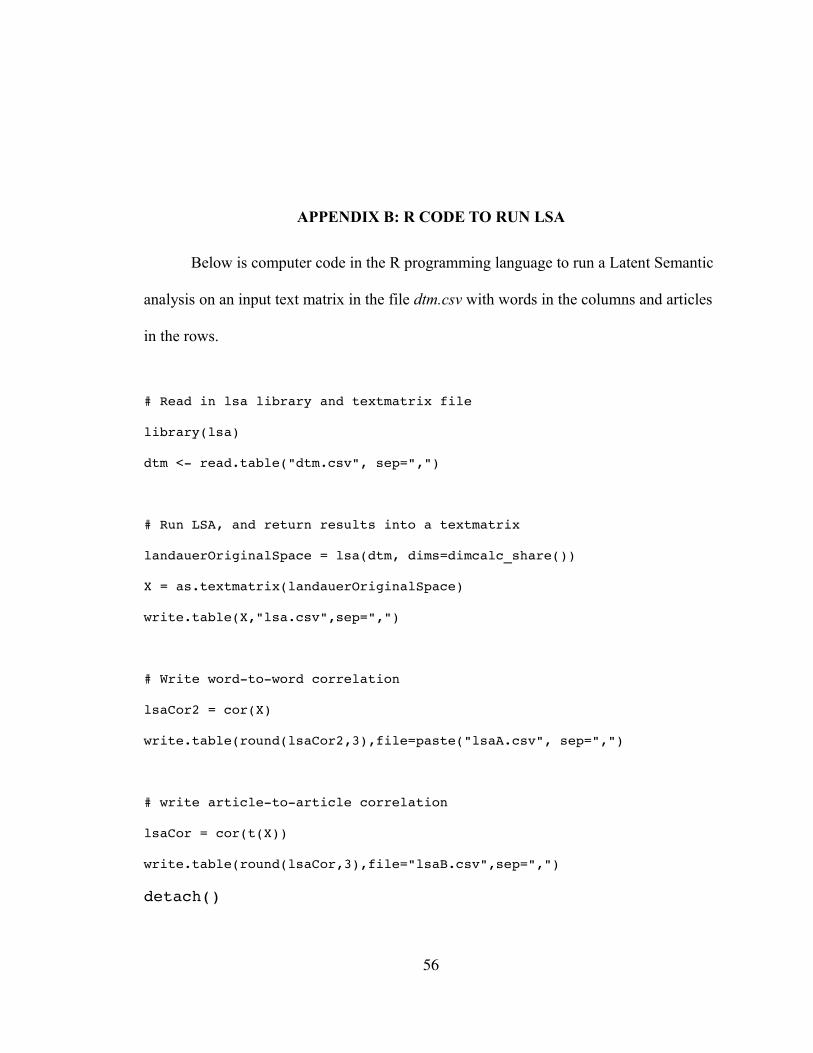
Below is computer code in the R programming language to run a Latent Semantic

analysis on an input text matrix in the file dtm.csv with words in the columns and articles

in the rows.

# Read in lsa library and textmatrix file

library(lsa)

dtm <­ read.table("dtm.csv", sep=",") 

# Run LSA, and return results into a textmatrix

landauerOriginalSpace = lsa(dtm, dims=dimcalc_share()) 

X = as.textmatrix(landauerOriginalSpace) 

write.table(X,"lsa.csv",sep=",") 

# Write word­to­word correlation

lsaCor2 = cor(X) 

write.table(round(lsaCor2,3),file=paste("lsaA.csv", sep=",") 

# write article­to­article correlation

lsaCor = cor(t(X)) 

write.table(round(lsaCor,3),file="lsaB.csv",sep=",") 

detach()

56

REFERENCE LIST

Barabasi, A.L., H. Jeong, Z. Neda, E. Ravasz, A. Schubert, T. Vicsek. 2002. Evolution of the social network of scientific collaborations. Physica A: 590­614.

Borner, Katy, Chaomei Chen, Kevin W. Boyack. 2003. Visualizing knowledge domains. Annual Review of Information Science and Technology 37: 179­255.

Chen, Chaomei. 1998. Generalised similarity analysis and pathfinder network scaling. Interacting with Computers 10: 107­128.

Chen, Chaomai. 1999. Visualizing semantic spaces and author co­citation networks in digital libraries. Information Processing and Management 35: 401­420.

Chen, Chaomai. 2005. Top 10 unsolved information visualization problems. IEEE Computer Graphics and Applications 25(4): 12­16.

Chen, Chaomai. 2006. Information Visualization: Beyond the Horizon, 2nd edition. Springer. London.

Chen, Chaomei, Jansa Kuljis, Ray J. Paul. 2001. Visualizing latent domain knowledge. IEEE Transactions on Systems, Man, and Cybernetics: Part C: Applications and Reviews 31(4): 518­529.

Chen, Chaomei, Timothy Cribbin, Robert Macredie, Sonali Moror. 2002. Visualizing and tracking the growth of competing paradigms: two case studies. Journal of the American Society for information Science and Technology 53 (8) : 678­689.

Chen, Chaomei, Il­Yeol Song, Weizhong Zhu. 2007. Trends in conceptual modeling: citation analysis of the ER conference papers (1979­2005). Proceedings of the 11th 

International Conference on the International Society for Scientometrics and Informatrics. CSIC, Madrid, Spain, June 25­27, 2007. pp. 189­200.

Chen, Chaomai, Jian Zhang, Weizhong Zhu, Michael Vogeley. 2007. Delineating the citation impact of scientific discoveries. JCDL  2007, Vancouver, British Columbia, Canada.

57

58

Chen, Chaoami, Weizhong Zhu, Brian Tomaszewski, Alan MacEachren. 2007. Tracing conceptual and geospatial diffusion of knowledge. Online Communities and Social Computing 265­274.

Deerwester, Scott, Susan T. Dumais, George W. Furnas, Thomas K. Landauer, Richard Harshman. 1990. Indexing by Latent Semantic Analysis. Journal of the American Society of Information Science 41(6): 391­407.

Elmes, Gregory. 2005. Guest Editorial: The University Consortium for Geographic Information Science: Shaping the Future at Ten Years. Transactions in GIS 9(3): 273­276.

Golub, Gene H., Charles F. Van Loan. 1996. Matrix Computation, 3rd edition. The John Hopkins University Press, Baltimore and London.

Hagerstrand, Torsten. 1967. Innovation Diffusion as a Spatial Process. Translated by Allen Pred. The University of Chicago Press, Chicago and London.

Kessler, M. M. 1963. Bibliographic coupling between scientific papers. American Documentation 14(1): 10­25.

Lewison, Grant. Isla Rippon, Steven Wooding. 2005. Downstream influence: tracking knowledge diffusion through citations. Research Evaluation1(1): 5­14.

Morris, Steven A. G., Yen, Zheng Wu, Benyam Asnake. 2003. Time line visualization of research fronts.  Journal of the American Society for Information Science and Technology 54(4): 413­422.

Newman, M. E. J. 2000. Who is the best connected scientist? A study of scientific coauthorship networks. Physics Review E 64: 16131­16132.

Newman, M. E. J. 2001. The structure of scientific collaboration networks. Proceedings of the National Academy of Science 98: 404­416.

Rogers, Everett M. 2003. Diffusion of Innovations, 5th edition. Free Press, New York.

Ryan, Bryce, Neal C. Gross. 1943. The Diffusion of Hybrid Seed Corn in Two Iowa Communities. Rural Sociology 8(1): 15­24.

Singh, Jasjit. 2005. Collaborative networks as determinants of knowledge diffusion patterns. Management Science 51(5): 756­770.

59

Small, Henry. 1973. Co­citation in the scientific literature: a new measure of the relationship between two documents. Journal of the American Society for Information Science 24(4): 265­269.

Small, Henry. 2003. Paradigms, citations, and maps of science: a personal history. Journal of the American Society for Information Science and Technology 54(5): 394­399.

Strang, David. Nancy Brandon Tuma. 1993. Spatial and temporal heterogeneity in diffusion. The American Journal of Sociology 99(3): 614­639.

Travers, Jeffrey, and Stanley Milgram. 1969. An Experimental Study of the Small World Problem. Sociometrics 3(4): 425­443.

University Consortium of Geographic Information Science. 1996. Research priorities for geographic information science. Cartography and Geographic Information Systems 23(3): 115­127.

University Consortium of Geographic Information Science. 1998. Research priorities for geographic information science. http://www.ucgis.org/, Accessed June 18, 2008.

University Consortium of Geographic Information Science. 1999. Research priorities for geographic information science. http://www.ucgis.org/, Accessed June 18, 2008.

University Consortium of Geographic Information Science. 2000. Research priorities for geographic information science. http://www.ucgis.org/, Accessed June 18, 2008.

University Consortium of Geographic Information Science. 2002. Research priorities for geographic information science. http://www.ucgis.org/, Accessed June 18, 2008.

University Consortium of Geographic Information Science. 2003. Informational Brochure. http://www.ucgis.org/, Accessed June 18, 2008.

University Consortium of Geographic Information Science. 2006. Research priorities for geographic information science. http://www.ucgis.org/, Accessed June 18, 2008.

Valente, Thomas W. 1995. Network Models of the diffusion of innovations. Hampton Press, Inc. Cresskill, New Jersey.

60

Valente, Thomas W. 1996. Social network thresholds in the diffusion of innovations. Social Networks 18: 69­89.

Valente, Thomas W., Robert K. Foreman. 1998. Integration and radiality: measuring the extent of an individual's connectedness and reachability in a network. Social  Networks 20: 89­105.

Watts, Duncan, and Steven Strogatz. 1998. Collective dynamics of 'small­world' networks. Nature 393: 440­442.

White, Howard D., Griffith, B. C. 1981. A cocitation map of authors in judgment and decision research. Journal for the American Society of Information Science 32: 163­172.

White, Howard D. 2003. Pathfinder networks and author cocitation analysis: a remapping of paradigmatic information scientists. Journal of the American Society for Information Science and Technology 54(5): 423­434.

Yang, Yiming, Christopher G. Chute. 1992. A Linear least squares fit mapping method for information retrieval from natural language texts. Proceedings of COLNIG­92, Nantes, France, August 23­28, 1992. 447­ 453.

VITA

David Aaron Parr was born on November 27, 1973 in Fort Smith, Arkansas. He 

entered Southern Methodist University, Dallas, Texas, in 1991 and  attained a Bachelor's 

of Science in Computer Science in 1996. He spent several months in the SMU­in­Oxford 

program at University College at Oxford, United Kingdom, in 1995. In Augst, 2004, he 

entered the Graduate College of Texas State University­San Marcos, Texas.

In addition to professional work as a computer programmer, systems analyst, and 

UNIX systems administrator from the years 1992 to 2008 at Texas Instruments, Dallas, 

Dallas Semiconductor, and the University of Texas at Austin, he has held a variety of odd 

jobs. These include a kindergarten teacher, radio disc jockey, goat herder, and celebrant. 

He has ordained two weddings in Texas and one in Missouri. He currently resides in 

Austin, Texas.

Permanent Address:  3517 North Hills Drive

Apt R205

Austin, TX 78731

This thesis was typed by the author.