Inhomogeneity-induced variance of cosmological parameters

Astronomy & Astrophysics manuscript no. curvaturevariance˙arXiv2 © ESO 2018November 1, 2018

Inhomogeneity-induced variance of cosmological parametersAlexander Wiegand and Dominik J. Schwarz

Fakultat fur Physik, Universitat Bielefeld, Universitatsstrasse 25, D–33615 Bielefeld, Germanye-mail: wiegand and dschwarz both at physik dot uni-bielefeld dot de

Preprint online version: November 1, 2018

Abstract

Context. Modern cosmology relies on the assumption of large-scale isotropy and homogeneity of the Universe. However, locally theUniverse is inhomogeneous and anisotropic. This raises the question of how local measurements (at the ∼ 102 Mpc scale) can be usedto determine the global cosmological parameters (defined at the ∼ 104 Mpc scale)?Aims. We connect the questions of cosmological backreaction, cosmic averaging and the estimation of cosmological parameters andshow how they relate to the problem of cosmic variance.Methods. We used Buchert’s averaging formalism and determined a set of locally averaged cosmological parameters in the contextof the flat Λ cold dark matter model. We calculated their ensemble means (i.e. their global value) and variances (i.e. their cosmicvariance). We applied our results to typical survey geometries and focused on the study of the effects of local fluctuations of thecurvature parameter.Results. We show that in the context of standard cosmology at large scales (larger than the homogeneity scale and in the linear regime),the question of cosmological backreaction and averaging can be reformulated as the question of cosmic variance. The cosmic varianceis found to be highest in the curvature parameter. We propose to use the observed variance of cosmological parameters to measure thegrowth factor.Conclusions. Cosmological backreaction and averaging are real effects that have been measured already for a long time, e.g. by thefluctuations of the matter density contrast averaged over spheres of a certain radius. Backreaction and averaging effects from scales inthe linear regime, as considered in this work, are shown to be important for the precise measurement of cosmological parameters.

Key words. Cosmology:theory, cosmological parameters, large-scale structure of Universe

1. Introduction

How do inhomogeneities in the matter distribution of theUniverse affect our conception of its expansion history and ourability to measure cosmological parameters? Typically, thesemeasurements rely on the averaging of a large number of in-dividual observations. In an idealised situation we can think ofthem as volume averages. To give an example, the power spec-trum, which is the Fourier–transformed two–point correlationfunction, may be seen as a volume average with weight eikx.Measurements of the properties of the large–scale structure relyon the observation of large volumes that have been pushed for-ward to ever higher redshifts in the last decade, from the two–degree Field survey (2dF, Colless et al. 2001) over the SloanDigital Sky Survey (SDSS, Abazajian et al. 2009) to the cur-rent WiggleZ (Drinkwater et al., 2010) and Baryon OscillationSpectroscopic Survey (BOSS, Eisenstein et al. 2011).

A theorem by Buchert states that the evolution of anyvolume-averaged comoving domain of an arbitrary irrota-tional dust Universe may be described by the equationsof a Friedmann–Lemaıtre–Robertson–Walker (FLRW) model,but driven by effective sources that encode inhomogeneities(Buchert, 2000, 2001). The consequences of this have beenstudied extensively in perturbation theory (Kolb et al., 2005;Li & Schwarz, 2007, 2008; Brown et al., 2009a,b; Larena,2009; Clarkson et al., 2009; Buchert et al., 2011) and for non-perturbative models (Buchert et al., 2006; Marra et al., 2007;Rasanen, 2008; Kainulainen & Marra, 2009; Roy & Buchert,2010). Apart from the ongoing debate to what extent the globalevolution is modified through backreaction effects from small-

scale inhomogeneities (Rasanen, 2004; Ishibashi & Wald, 2006;Kolb et al., 2006; Buchert, 2008; Buchert et al., 2009; Wiegand& Buchert, 2010), Li & Schwarz (2008) showed that the mea-surement of cosmological parameters is limited by uncertaintiesconcerning the relation between observable locally and unob-servable globally averaged quantities.

In contrast to the well–studied cosmic variance of the cosmicmicrowave background, which is most relevant at the largest an-gular scales, the theoretical limitation on our ability to predictobservations at low redshift arises not only from the fact that weobserve only one Universe, but also from the fact that we samplea finite domain (much smaller than the Hubble volume). Bothlimitations contribute to the cosmic variance. This is differentfrom the sampling variance caused by shot noise, i.e. the limita-tion of the sampling of a particular domain because of the finitenumber of supernovae (SN) or galaxies observed. In the era ofprecision cosmology, the errors caused by cosmic variance maybecome a major component of the error budget.

The purpose of this work is to demonstrate that the questionsof cosmic averaging, cosmological backreaction, and the prob-lems of cosmic variance and parameter estimation are closelylinked. We demonstrate that cosmic variance is actually one ofthe aspects of cosmological backreaction.

There have already been many studies on the effect of thelocal clumpiness on our ability to measure cosmological param-eters. However, they focused mainly on the fluctuations in thematter density and on the variance of the Hubble rate. The for-mer question has gained renewed interest in view of deep red-shift surveys such as GOODS (Giavalisco et al., 2004), GEMS(Rix et al., 2004) or COSMOS (Scoville et al., 2007). Because

1

arX

iv:1

109.

4142

v2 [

astr

o-ph

.CO

] 1

8 Fe

b 20

12

A. Wiegand, D.J. Schwarz: Inhomogeneity-induced variance of cosmological parameters

the considered survey fields are small, the variance of the matterdensity is an important ingredient in the error budget and it hasbeen found to be in the range of 20% and more, demonstratedempirically in SDSS data by Driver & Robotham (2010) andcalculated numerically from linear perturbation theory in Mosteret al. (2010).

The variance of the Hubble rate has been considered in thesetup of this work, i.e. first order linear perturbation theory incomoving synchronous gauge, in Li & Schwarz (2008). A calcu-lation of the same effect in Newtonian gauge has been performedin Clarkson et al. (2009) and Umeh et al. (2010); the two meth-ods agree. Calculations of the fluctuations in the Hubble rate ow-ing to peculiar velocities alone have a longer history (Kaiser,1988; Turner et al., 1992; Shi et al., 1996; Wang et al., 1998).The effects of inhomogeneities on other cosmic parameters havebeen studied in Newtonian cosmology (Buchert & Ehlers, 1997;Buchert et al., 2000).

There has been less activity in studying the effects of thethird important player besides number density and Hubble ex-pansion: cosmic curvature. Even if the Universe is spatially flat,as expected by the scenario of cosmological inflation and con-sistent with the observations of the temperature anisotropies ofthe cosmic microwave background, the local curvature may bequite different. To answer the question how big this differenceactually is for realistic survey volumes, we here extend the anal-ysis of Li & Schwarz (2007, 2008), where these effects havebeen estimated for the first time. For the spatially flat Einstein-de Sitter (EdS) model, the averaged curvature parameter ΩD

Rhas

been shown to deviate from zero by ∼ 0.1 on domains at the100 Mpc scale.

Here we adapt the analysis of Li & Schwarz (2008) to thecase of a ΛCDM universe, introduce a more realistic power spec-trum and use observationally interesting window functions, notrestricted to full–sky measurements.

There has been quite some confusion about the choice ofgauge and the dependence of the averaged quantities on it.Recently it has been shown (Gasperini et al., 2010) that this isnot a problem if one consistently works in one gauge and thenexpresses the quantity that is finally observed in this frame aswell. This is easier in some gauges than in others, but the resultis (as expected) the same, as is also confirmed explicitly by thefact that our results are consistent with those of Clarkson et al.(2009) and Umeh et al. (2010), obtained in Newtonian gauge.The quest for simplicity explains our choice to use comovingsynchronous gauge, because this is the frame that is closest tothe one used by the observers.

Fig. 1 depicts the theorist’s and the observer’s view on theUniverse in a schematical way. It points out that in the end itis the average quantities that we are interested in, but that in anintermediate step, observers like to think of the objects they mea-sure to lie in a comoving space with simple Euclidian distances.The comoving synchronous gauge, which has a clear notion of”today” for a fluid observer sitting in a galaxy as we do, helps todefine the things observers measure in a simple way.

In Section 2 we establish the conceptual framework for thestudy of effects of inhomogeneities on observable quantities.Section 3 and 4 generalize some of the results of Li & Schwarz(2007, 2008) and Li (2008) from an Einstein–de Sitter (EdS)to a ΛCDM background and implement a more realistic mat-ter power spectrum. Section 5 investigates the effects of variouswindow functions, again extending the analysis of Li & Schwarz(2008); Li (2008). Section 6 concentrates on deriving the mag-nitude of curvature fluctuations for realistic window functions.Section 7 applies the formalism to the local distance measure

Figure 1. Comparison of the theorist’s and observer’s view onthe Universe. Our calculation in comoving synchronous gaugefacilitates the description of the boundaries of the experimen-tally investigated regions in our Universe. Note, that recentlythere have been attempts by Bonvin & Durrer (2011) to directlyrelate the two upper circles. This was done by calculating thepredictions for the quantities in redshift space explicitly fromthe perturbed ΛCDM model.

DV , determined in the observation of baryonic acoustic oscil-lations (BAO). Section 8 is a remark on the link between thevariance of averaged expansion rates at different epochs and thebackground evolution, before we conclude in Section 9.

2. Inhomogeneity and expansion

We assume that the overall evolution of the Universe is describedby a flat ΛCDM model, which we adopt as our backgroundmodel throughout this work. Global spatial flatness does not pre-vent the local curvature to deviate from zero.

The distribution of nearby galaxies indicates that the scalesat which the Universe is inhomogeneous reach out to at least100 Mpc. Above these scales it is not yet established if thereis a turnover to homogeneity, as was claimed in Hogg et al.(2005), or if the correlations in the matter distribution merelybecome weaker, but persist up to larger scales, as is discussedin Labini (2010). At least morphologically, homogeneity has notbeen found up to scales of about 200 Mpc (Kerscher et al., 1998,2001; Hikage et al., 2003).

2


Consequently, we need a formalism that is applicable in thepresence of inhomogeneities at least for the description of thelocal expansion. This may be accomplished considering spa-tial domainsD and averaging over their locally inhomogeneousobservables (Buchert, 2000, 2001). Technically one performsa 3+1 split of spacetime. Because we considered pressurelessmatter only, we chose a comoving foliation in which the spa-tial hypersurfaces are orthogonal to the cosmic time. This meansthat the formalism will not be able to take into account light-cone effects. Therefore, it is well adapted for regions of the uni-verse that are not too extended, a notion described more pre-cisely in Sect. 5. The equations then describe the evolution ofthe volume of the domain D, given by |D|g :=

∫D

dµg, wheredµg := [(3)g (t, x)]1/2d3x and (3)g is the fully inhomogeneousthree–metric of a spatial slice.

To obtain an analogy to the standard Friedmann equations,one defines an average scale factor from this volume

aD (t) :=(|D|g

|D0|g

) 13

, (1)

where the subindex 0 denotes ”today”, as throughout the restof this work. The definition implies aD0 = 1. In analogy to thebackground model HD := aD/aD. The foliation may be used todefine an average over a three–scalar observable O on a domainD in the spatial hypersurface

〈O〉D (t) :=

∫D

O (t, x) dµg∫D

dµg. (2)

Examples for these observables include the matter density % orthe redshift z of a group of galaxies in the domainD.

The scalar parts of Einstein’s equations for an inhomoge-neous matter source become evolution equations for the volumescale factor driven by quantities determined by this average:

3aDaD

= −4πG 〈%〉D + QD + Λ, (3)

3H2D = 8πG 〈%〉D −

12〈R〉D −

12QD + Λ, (4)

0 = ∂t 〈%〉D + 3HD 〈%〉D . (5)

The expansion of the domain D is determined by the averagematter density, the cosmological constant, the average intrinsicscalar curvature 〈R〉D and the kinematical backreaction QD. Thelatter encodes the departure of the domain from a homogeneousdistribution and is a linear combination of the variance of theexpansion rate and the variance of the shear scalar.

Equations (3) to (5) mean that the local evolution of any in-homogeneous domain is described by a set of equations that cor-responds to the Friedmann equations.

The cosmic parameters, defined by

ΩDm :=8πG3H2D

〈%〉D , ΩDΛ :=Λ

3H2D

, (6)

ΩDR

:= −〈R〉D

6H2D

, ΩDQ

:= −QD

6H2D

,

are domain–dependent. Owing to the fluctuating matter density,the curvature and the average local expansion rate will also fluc-tuate. When we constrain ourselves to the perturbative regime,the modification due to QD is important on scales of the order of10 Mpc (Li & Schwarz, 2008).

Here we are interested to see to what extent the values of theparameters (6) vary if we look at different domains of size D inthe Universe. We could therefore define an average over manyequivalent domains D at different locations in our current spa-tial slice. For an ergodic process, however, this is the same as thevariance of an ensemble average over many realizations of theUniverse keeping the domain D fixed, but changing the initialconditions of the matter distribution. This is the quantity that wecalculate in theory and therefore we have to rely on the assump-tion of ergodicity when comparing our results with the observa-tion. In our case this ensemble average is taken over quantitiesthat are volume averages. This means that for any observable Othere are two different averages involved. The domain averag-ing, 〈O〉D, and the ensemble average, O. We assume that bothaveraging procedures commute.

The fluctuations are then characterized by the variance withrespect to the ensemble averaging process,

σ(〈O〉D

):=

(〈O〉2D − 〈O〉D

2) 1

2. (7)

An example for a common observable calculated in this man-ner would be σ8 as the ensemble r.m.s. fluctuation of the matterdensity field. To quantify these fluctuations of a general observ-able O, we use the theory of cosmological perturbations. In Li& Schwarz (2007) it has been shown that to linear order, theQD–term in equations (4) and (3) vanishes. 〈%〉D, 〈R〉D and HDhowever, have linear corrections.

Furthermore, Li (2008) argued that there is no second–ordercontribution to the fluctuations for Gaussian density perturba-tions if their linear contributions are finite. This may be seenby decomposing the observable O into successive orders O =

O(0) + O(1) + O(2) + · · ·. It is usually assumed that O(1) = 0. Now,for Gaussian perturbations only terms of even order give rise tonon-trivial contributions. Therefore, (7) may be expressed as

σ (O) =

√(O(1))2

1 +

(O(2))2

−(O(2)

)2+ 2O(1)O(3)

2(O(1))2

, (8)

which shows that the correction to the leading order linear termis already of third order. This is why we content ourselves for theevaluation of the fluctuations in the parameters 〈%〉D, 〈R〉D andHD or ΩDm , ΩD

Rand HD to a first order treatment. This argument

does not apply if(O(1))2

= 0, as is the case for QD. In that caseQD and σ(QD) are of second order in perturbation theory.

3. Cosmological parameters and their mean fromlocal averaging

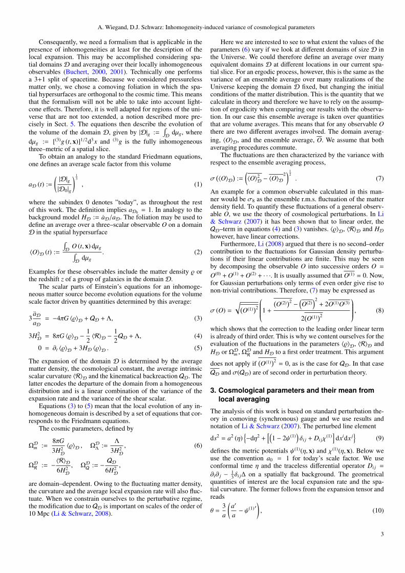
The analysis of this work is based on standard perturbation the-ory in comoving (synchronous) gauge and we use results andnotation of Li & Schwarz (2007). The perturbed line element

ds2 = a2 (η)−dη2 +

[(1 − 2ψ(1)

)δi j + Di jχ

(1)]

dxidx j

(9)

defines the metric potentials ψ(1)(η, x) and χ(1)(η, x). Below weuse the convention a0 = 1 for today’s scale factor. We useconformal time η and the traceless differential operator Di j =

∂i∂ j −13δi j∆ on a spatially flat background. The geometrical

quantities of interest are the local expansion rate and the spa-tial curvature. The former follows from the expansion tensor andreads

θ =3a

(a′

a− ψ(1)′

), (10)

3


where ()′ stands for the derivative with respect to conformaltime. Calculating the spatial Ricci curvature from the above met-ric yields

R =12a2

(2

a′

aψ(1)′ + ψ(1)′′

). (11)

By the covariant conservation of the energy momentum tensor,ψ(1) is related to the matter density contrast

δ (η, x) :=ρ(1)

ρ(0) (12)

by

ψ(1) =13δ − ζ (x) , (13)

with ζ (x) denoting a constant of integration. This constant playsno role in the following, because θ and R involve only timederivatives of ψ(1).

For dust and a cosmological constant, Einstein’s equationsgive the well–known relation

δ′′ +a′

aδ′ =

4πGρ(0)0

aδ, (14)

at first order in perturbation theory. For the ΛCDM model thesolution reads [see, e.g. Green et al. (2005)]

δ (a, x) =D (a)D (1)

δ0(x), (15)

where δ0 (x) is the density perturbation today. D (a) is the growthfactor given by

D (a) = a 2F1

(1,

13

;116

;−ca3), with c ≡

ΩΛ

Ωm(16)

and 2F1 is a hypergeometric function. In the following we denotetoday’s value of the growth factor by D0 ≡ D (1).

Plugging this solution into (10) and using (13), we find thelocal expansion rate

13θ(a, x) = H0

√Ωm

a3

√1 + ca3

(1 −

13

f (a) δ (a, x)), (17)

expressed in terms of the growth rate

f (a) :=d ln D (a)

d ln a=

5 aD(a) − 3

2(1 + ca3) . (18)

From (11) we find the local spatial curvature

R(a, x) = 101a2 H2

0Ωmδ0(x)D0

. (19)

From these quantities we can define local Ω functions,

Ωm (a, x) =1

1 + ca3

[1 +

(1 +

23

f (a))δ (a, x)

], (20)

ΩR (a, x) = −

[1

1 + ca3 +23

f (a)]δ (a, x) , (21)

ΩΛ (a, x) =ca3(

1 + ca3) [1 +

23

f (a) δ (a, x)], (22)

ΩQ (a, x) = 0, (23)

demonstrating that the importance of curvature effects growsproportional to the formation of structures. A remarkable prop-erty is that

∑Ωi(a, x) = 1 holds not only for the FLRW back-

ground, but also at the level of perturbations. For linear pertur-bations the kinematic backreaction term does not play any role,but becomes important as soon as quadratic terms are consid-ered.

Let us now compare these local quantities with the domain-averaged expansion rate and the spatial curvature (Li & Schwarz,2008). From the definition of the average 〈〉D in (2) we find that,in principle, fluctuations in the volume element dµg have to betaken into account. Writing dµg = Jd3x with the functional de-terminant J = a3

(1 − 3ψ(1)

), the average over the perturbed hy-

persurface agrees with an average over an unperturbed Euclideandomain⟨

O(1)⟩D

=

∫D

O(1)Jdx∫D

Jdx'

∫D

O(1)dx∫D

dx=:

⟨O(1)

⟩, (24)

if we restrict our attention to linear perturbations.We express domain-averaged quantities in terms of the vol-

ume scale factor aD, because we assume that the measured red-shift in an inhomogeneous universe is related to the average scalefactor. This has been advocated by Rasanen (2009), where therelation

(1 + z) ≈ a−1D (25)

has been established. Note that in principle one would have tointroduce averaging on some larger scale thanD to connect thisbackground average on some domain B to the redshift. For thesake of simplicity, and because we content ourselves with smallredshifts, we use the same domain D. This limits the validity ofthe result to small redshifts.

In order to relate a and aD, we start from

HD =13〈θ〉D =

aDaD

=1a

a′D

aD=

1a

(a′

a−

⟨ψ(1)′

⟩). (26)

To first order this relation gives

aD = a(1 −

13

(〈δ (a)〉D − 〈δ (1)〉D

)). (27)

We finally obtain the averaged Hubble rate

HD = H0

√Ωm

a3D

√1 + ca3

D

1 − 5 aDD(aD) − 3 D0

D(aD)

6(1 + ca3D

)D(aD)

D0〈δ0〉D

(28)

and the averaged spatial curvature

〈R〉D = 10 ΩmH2

0

a2D

〈δ0〉D

D0. (29)

For later convenience we also define the function

fD (aD) :=5 aD

D0− 3

2(1 + ca3D

), (30)

which is our modified version of the growth rate of Eq. (18),multiplied by D (a) /D0. It basically encodes the deviation of thetime evolution of the Hubble perturbation from the time evolu-tion of the ensemble averaged Hubble rate

HD (aD) = H0

√Ωm

a3D

√1 + ca3

D, (31)

4


as may be seen from the resulting expression

HD = HD (aD)(1 −

13

fD (aD) 〈δ0〉D

). (32)

In the Einstein-de Sitter limit (c→ 0 and Ωm → 1) we arriveat

HD =H0

a3/2D

(1 −

13

aD 〈δ0〉D

), (33)

〈R〉D = 10H2

0

a2D

〈δ0〉D . (34)

In order to compare this with the results of Li & Schwarz (2007,2008), we define the peculiar gravitational potential ϕ (x) via

∆ϕ (x) ≡ 4πGρ(1)a2 =32

H20δ

a=

23

1t20

δ

a(35)

and obtain

HD =2

3t0a−3/2D

[1 −

12

aDt20 〈∆ϕ〉

](36)

and

〈R〉D =203

a−2D 〈∆ϕ〉 . (37)

While our results agree for the spatial curvature, HD is differ-ent from the result in Li & Schwarz (2008), because there theassumption a 1 was made when applying (27).

Let us now turn to the dimensionless ΩD-parameters. To firstorder, they may be expressed as

ΩDm (aD) =1

1 + c a3D

[1 +

(1 +

23

fD (aD))〈δ0〉D

], (38)

ΩDR

(aD) = −

11 + c a3

D

+23

fD (aD) 〈δ0〉D , (39)

ΩDΛ (aD) =c a3D

1 + ca3D

[1 +

23

fD (aD) 〈δ0〉D

], (40)

ΩDQ

(aD) = 0. (41)

When taking the limit D → 0 in Eqs. (38) – (41), we recoverthe point-wise defined Ω-parameters of Eqs. (20) – (23). Thisprovides a self-consistency check of the averaging framework.

From the expressions for the ΩD-parameters one can eas-ily calculate the ensemble averages and the ensemble variance.〈δ0〉D = 0, since the domain-averaged overdensity ofD, in gen-eral non-zero, averages out when we consider a large number ofdomains of given size and local density fluctuations drawn fromthe same (Gaussian) distribution.

Here we adopt the common view that linear theory is agood description of the present universe at the largest observablescales (which has been questioned recently in Rasanen 2010).We then find the ensemble average of the curvature parameterΩDR

to vanish. For the matter density parameter Eq. (38) yields

ΩDm (aD) =(1 + c a3

D

)−1. (42)

This may be used to verify that the relation ΩDm + ΩDΛ

= 1 holds.

In addition, this relation implies that ΩDm(aD0

)corresponds to

today’s background matter density parameter:

ΩDm(aD0

)= Ωm + O

(⟨δ2

0

⟩D

). (43)

However, this is true at first order in the density contrast only,because in this case ensemble averages agree with backgroundquantities. At higher orders, the ensemble averages differ fromthe background quantities.

4. Variances of locally averaged cosmologicalparameters

After having convinced ourself that the expectations of the av-eraged ΩD-parameters are identical to their ΛCDM backgroundvalues up to second–order corrections, we now turn to the studyof their ensemble variances.

All variances of domain averaged cosmological parameterscan be related to the variance of the overdensity of the matterdistribution, σ

(〈δ0〉D

).

In order to specify 〈δ0〉D, we introduce the normalized win-dow function WD (X) and write

〈δ0〉D =

∫R3δ0 (x) WD (x) d3x

=

∫R3δ0 (k) WD (k) d3k, (44)

A tilde denotes a Fourier–transformed quantity. With the defini-tion of the matter power spectrum

δ0 (k) δ0 (k′) = δDirac (k + k′

)P0 (k) , (45)

where δDirac denotes Dirac’s delta function, the ensemble vari-ance of the matter overdensity becomes

(σD0

)2 := σ2 (〈δ0〉D

)=

∫R3

P0 (k) WD (k) WD (−k) d3k. (46)

For a spherical window function, this expression is the well–known matter variation in a sphere, often used to normalize thematter power spectrum by fixing its value for a sphere with aradius of 8h−1Mpc (σ8). To calculate this variance, we assumea standard ΛCDM power spectrum in the parametrization ofEisenstein & Hu (1998). Knowing σD at a particular epoch ofinterest, we can calculate all the fluctuations in the cosmic pa-rameters. They read:

δHD =13

HD (aD) fD (aD)σD0 , (47)

δΩDm = ΩDm (aD)(1 +

23

fD (aD))σD0 , (48)

δΩDR

= ΩDm (aD)

1 +23

fD (aD)

ΩDm (aD)

σD0 , (49)

δΩDΛ = ΩDΛ

(aD)23

fD (aD)σD0 , (50)

δΩDQ

= O((σD0

)2), (51)

where e.g. δΩDΛ

denotes the square root of the variance, δΩDΛ

:=

σ(ΩD

Λ

). ΩDm , HD and fD (aD) were defined in Eq. (42), (31) and

(30) and ΩDΛ

= 1 −ΩDm .These variances are the minimum ones that one can hope to

obtain by measurements of regions of the universe of size D.They do not include any observational uncertainties, nor biasingor sampling issues. They are intrinsic to the inhomogeneous darkmatter distribution that governs the evolution of the Universe.

5


Figure 2. The two survey geometries considered (separately). Asimple cone with one single opening angle α and a slice givenby two angles β and γ.

Equations (47) to (51) are interesting in two respects: Firstly,our expression for δHD is simpler than the one in Umeh et al.(2010), nevertheless, both results agree. Secondly, Eqs. (47) to(51) quantify the connection between fluctuations in cosmologi-cal parameters and inhomogeneities in the distribution of matter.If we choose ”today” as our reference value, Eqs. (47) to (50) al-low us to predict the domain averaged cosmological parameters:

HD = H0 ±13 H0 fD0 σD0

ΩDm = Ωm ± Ωm

(1 + 2

3 fD0

)σD0

ΩDR

= 0 ±(Ωm + 2

3 fD0

)σD0

ΩDΛ

= ΩΛ ±23 ΩΛ fD0 σD0

(52)

with

fD0 ≡ fD(aD0

)=

Ωm

2

(5D−1

0 − 3)≈

0.5 ΛCDM1.0 EdS , (53)

where we assumed Ωm = 0.3 for ΛCDM. More generally, forΩm > 0.1, fD0 may be approximated by (Lahav et al., 1991;Eisenstein & Hu, 1998)

fD0 ≈1

140

(2 + 140 Ω4/7

m −Ωm −Ω2m

). (54)

From the knowledge of σD0 we may therefore easily derivethe variation of cosmological parameters. To relate our calcula-tions to real surveys, we elaborate in the next section on how tocalculate σD0 for several survey geometries.

5. The effect of the survey geometry

Observations of the universe are rarely full–sky measurementsand typically sample domains much smaller than the Hubblevolume. We therefore must address the problem of the surveygeometry. Effects from a limited survey size are in particular im-portant for deep fields, as studied for example in Moster et al.(2010). While in their case, for small angles and deep surveys,approximating the observed volume by a rectangular geometry isappropriate, it probably is not appropriate for the bigger surveyvolumes that we have in mind.

We therefore chose two different geometries that resembleobservationally relevant ones. Firstly, we used a simple conewith a single opening angle α. The second geometry is a slicedescribed by two angles β and γ for the size in right ascension

Volume Hh0.73 Mpc3L

ΣD

in%

Figure 3. Variance of the matter density, σD, as a function ofthe observed domain volume. Data were derived from the SDSSmain sample by Driver & Robotham (2010). The dashed (red)line shows the fit of Driver & Robotham (2010) to the data,the solid (green) line is our result including the sample variance[solid (blue) line at the bottom].

and declination respectively. In the radial direction we assumeda top hat window, whose cut–off value corresponds to the depthof the survey. Both shapes are shown in Fig. 2.

To calculate σD0 for both geometries, we used a decompo-sition into spherical harmonics. This allowed us to derive an ex-pression for the expansion coefficients in terms of a series incos (2nα) for the cone and a similar one for the slice, dependingon trigonometric functions of β and γ. The radial coefficientswere calculated numerically using the ΛCDM power spectrumof Eisenstein & Hu (1998), including the effect of baryons onthe overall shape and amplitude of the matter power spectrum,but without baryon acoustic oscillations.

All plots use best-fit ΛCDM values as given in Komatsu et al.(2011); Ωb = 0.0456, Ωcdm = 0.227 and ns = 0.963. The powerspectrum is normalized to σ8 = 0.809.

To ensure that the result of our calculation for the slice-like geometry and a standard ΛCDM power spectrum is reason-able, we compared it with an analysis of SDSS data by Driver& Robotham (2010). In Fig. 3 we show this comparison oftheir r.m.s. matter overdensity σD obtained from the SDSS maingalaxy sample, in terms of its angular extension (and hence thevolume). The dashed line going through the points shows theirempirical fit to the data. The solid green line shows our result forthe cosmic variance of a slice with respective angular extension(for β = γ), plus their sample variance. Note that our result isnot a fit to SDSS data, but is a prediction based on the WMAP7yr data analysis. Additionally, the real SDSS window functionis slightly more complicated than our simplistic window, thusperfect agreement is not to be expected.

For the full SDSS volume, σD0 is shown in Fig. 4. For com-parison we also added the smaller, southern hemisphere 2dFsurvey and a hypothetical full sky survey. For the two surveys,we assumed an approximate angular extension of 120°×60° for

6


0.05 0.10 0.15 0.20 0.25 0.30 0.35

0.51.0

5.010

50

redshift z

ΣHzL

in%

2dF

SDSS

Full sky

Figure 4. Variance of the matter density, σD, for survey geome-tries resembling the 2dFGRS, the SDSS and a hypothetical fullsky survey as a function of maximum redshift considered. Wefind that the determination of the local σD below redshifts of0.1 (corresponding to ∼ 400 Mpc) is fundamentally limited bycosmic variance to the 1% level.

SDSS and for the two fields of the 2dF survey 80°×15° and75°×10°. The ongoing BOSS survey corresponds to the plot forthe SDSS geometry because it will basically have the same an-gular extension. Because it will target higher redshifts, it is notin the range of our calculation, however. As a rough statement(the precise value depends on the redshift), one may say thatthe 2dF survey is a factor of 5 and the SDSS survey a factor of2.5 above the variance of a full sky survey. This is interestingbecause the SDSS survey covers approximately only 1/6 of thefull sky and the 2dF survey only 1/20. This is due to the angulardependence of σD. We find that fluctuations drop quickly as weincrease small angles and flattens at large angles.

From Fig. (4) we see that the cosmic variance of the matterdensity for the SDSS geometry is 5% at a depth of z ≈ 0.08 andstill 1% out to z ≈ 0.23. Note, however, that the extension ofthe domain of (spatial) averaging to a redshift of 0.35 is clearlynot very realistic because lightcone effects will become relevantwith increasing extension of the domain. The assumption thatthis domain would be representative for a part of the hypersur-face of constant cosmic time becomes questionable. We expect,however, that in this range evolution effects will only be a minorcorrection to the result presented here because of the followingestimation:

The main effect we miss by approximating the lightcone bya fixed spatial hypersurface is evolution in the matter densitydistribution. To specify what ”region that is not too extendedspatially” means, one should therefore estimate the maximumevolution in a given sample. This can be done by determiningthe growth of the density contrast in the outermost (and there-fore oldest) regions of the sample. In the linear regime con-sidered here, the evolution of the density contrast is given byδ (z) = δ0D (0) /D (z). Therefore, lightcone corrections shouldbe smaller than εl = 1−D (z) /D (0) which is εl ≈ 5% for z = 0.1and εl ≈ 14% for z = 0.3. Therefore, the order of magnitudeof our results should be correct on a wider range of scales, buton scales above z = 0.3 the corrections to our calculation areexpected to pass beyond 15%.

Finally, it should be noted that for large volumes the actualshape of the survey geometry is not very important. As longas all dimensions are bigger than the scale of the turnover of

the power spectrum, the deviation of the cosmic variance forour shapes, compared to those of a box of equal volume, is atthe percent level. To reach this result, we compared σD0 forthe slice–like geometry to its value for a rectangular box of thesame volume. We used a slice for which β = γ. The box wasconstructed to have a quadratic basis and the same depth as theslice in radial direction. Therefore the base square of the boxis smaller than the square given by the two angles of the slice.The result of this comparison is that the deviation of σrect

D0from

the value for the slice is at most 6% for angles above β ≈ 10°.For smaller angles the deviation becomes bigger and redshift–dependent. This is caused by the changing shape of the powerspectrum at small scales. The large angle behavior confirms anobservation of Driver & Robotham (2010). They found that thecosmic variance in the SDSS dataset was the same for both ofthe two geometries they considered.

6. Fluctuations of the curvature parameter

After the general study of the effect of the shape of the observa-tional domain D on σD0 , one may ask for which parameter thefluctuations are most important.

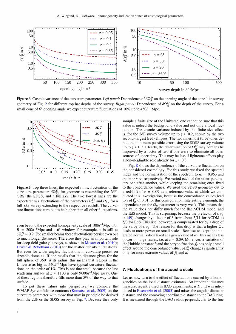
The three lowest lines in the plot of Fig. 5 show that thisis the case for the curvature fluctuations. The two lowest lines,showing the fluctuations δΩm and δHD0/HD0 for the full sphere,lie a factor of 1.6 and 3.8, respectively, below the respective cur-vature fluctuations δΩD

R. Therefore the fluctuations of Ωm play

a smaller role for all universes with Ωm < 1. The uncertainty inHD0 , which has been in the focus of the investigations so far (Shiet al., 1996; Li & Schwarz, 2008; Umeh et al., 2010), contributeseven less to the distortion of the geometry, as we shall discuss inSection 7.

What this means for real surveys, such as the 2dF or theSDSS survey, is shown by the three upper lines in Fig. 5. Theycompare δΩD

Rfor the slices observed by these surveys to that

of a full sky measurement. δΩDR

is bigger than one percent upto a redshift of 0.18 for the SDSS and 0.28 for the 2dF surveyand it does not drop below 0.001 for values of z as high as 0.5.This may seem very low, but it has been shown that getting thecurvature of the universe wrong by 1h already affects our abil-ity to measure the dark energy equation of state w (z) (Clarksonet al., 2007). Of course one has to keep in mind that for highredshifts one has to be careful with the values presented here be-cause they are based on the assumption that the observed regionlies on one single spatial hypersurface. Because this approxima-tion worsenes beyond a redshift of 0.1, there may be additionalcorrections to the size of the fluctuations stemming from light-cone effects.

To investigate the curvature fluctuations for more general ge-ometries, we show in Fig. 6 the angular and radial dependenceof the curvature fluctuation δΩD

R(α) for the cone-like window of

Fig. 2.On the l.h.s. of Fig. 6 we evaluate the angular dependence.

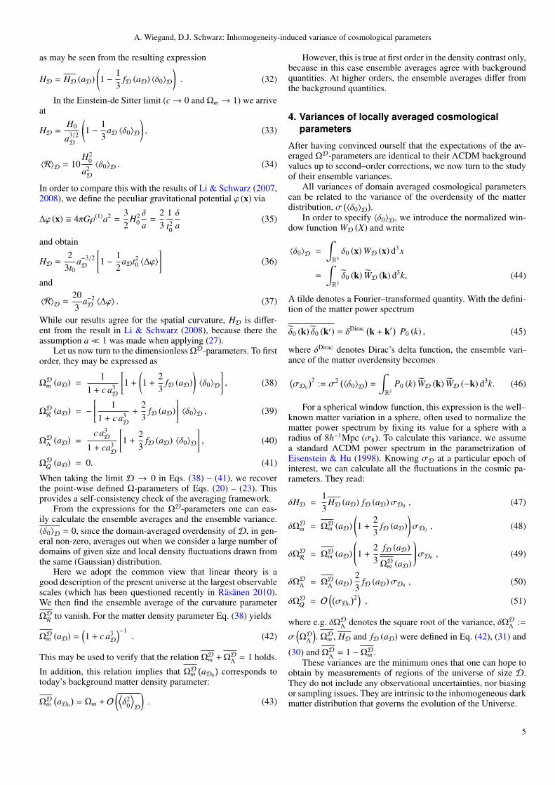
For a survey that only reaches a redshift of 0.1, the fluctuationsare still higher than 0.01 for a half–sky survey. It is interesting tonote that for a deeper survey, δΩD

R(α) grows much faster when

α is reduced than for a shallow survey. This is because σD0 (R)changes from a relatively weak R−1 decay to a R−2 decay onlarger scales. For z = 0.35, this behavior dominates and a de-crease in α increases σD0 (R, α) stronger than in the R−1 regime.

On the r.h.s. of Fig. 6 we show the dependence of δΩDR

on the survey depth for some opening angles of the cone-likewindow. For narrow windows the fluctuation in ΩD

Rstays high,

7


50 100 150 200 250 300 350

0.51.0

5.010

50100

opening angle in °

∆W

RDin

%

z = 0.05

z = 0.1

z = 0.2

z = 0.35

10 50 100 500

0.5

1.0

5.0

10

50

100

survey depth in h-1Mpc

∆W

RDin

%

Α = 6°

Α = 30°

Α = 90°

Α = 360°

Figure 6. Cosmic variance of the curvature parameter. Left panel: Dependence of δΩDR

on the opening angle of the cone-like surveygeometry of Fig. 2 for different top hat depths of the survey. Right panel: Dependence of δΩD

Ron the depth of the survey. For a

small cone of 6° opening angle we expect curvature fluctuations of 10% up to 450h−1Mpc.

Figure 5. Top three lines: the expected r.m.s. fluctuation of thecurvature parameter, δΩD

R, for geometries resembling the 2dF-

GRS, the SDSS, and a full sky. The two lowest lines are theexpected r.m.s. fluctuations of the parameters Ω

D0m and HD0 for a

full–sky survey extending to the respective redshift. The curva-ture fluctuations turn out to be higher than all other fluctuations.

even beyond the expected homogeneity scale of 100h−1Mpc. ForR = 200h−1Mpc and a 6° window, for example, it is still atδΩDR≈ 0.2. For smaller beams these fluctuations persist even out

to much longer distances. Therefore they play an important rolefor deep field galaxy surveys, as shown in Moster et al. (2010);Driver & Robotham (2010) for the matter density fluctuations.But even for wider angles, fluctuations in curvature persist onsizeable domains. If one recalls that the distance given for thefull sphere of 360° is its radius, this means that regions in theUniverse as big as 540h−1Mpc have typical curvature fluctua-tions on the order of 1%. This is not that small because the lastscattering surface at z ≈ 1100 is only 9600h−1Mpc away. Oneof these regions therefore fills more than 5% of the way to thatsurface.

To put these values into perspective, we compare theWMAP 5yr confidence contours (Komatsu et al., 2009) on thecurvature parameter with those that may in principle be derivedfrom the 2dF or the SDSS survey in Fig. 7. Because they only

sample a finite size of the Universe, one cannot be sure that thisvalue is indeed the background value and not only a local fluc-tuation. The cosmic variance induced by this finite size effectis, for the 2dF survey volume up to z ≈ 0.2, shown by the twosecond–largest (red) ellipses. The two innermost (blue) ones de-pict the minimum possible error using the SDSS survey volumeup to z ≈ 0.3. Clearly, the determination of ΩD

Rmay perhaps be

improved by a factor of two if one were to eliminate all othersources of uncertainty. This may be less if lightcone effects playa non–negligible role already for z ≈ 0.3.

Fig. 8 shows the dependence of the curvature fluctuation onthe considered cosmology. For this study we fixed the spectralindex and the normalization of the spectrum to ns = 0.963 andσ8 = 0.809, respectively. We varied each of the other parame-ters one after another, while keeping the remaining ones fixedto the concordance values. We used the SDSS geometry out toa redshift of z = 0.09 as a reference value at which we con-ducted this investigation, because the concordance values leadto a δΩD

Rof 0.01 for this configuration. Interestingly enough, the

dependence on the Ωm parameter is very weak. This means thatthe value does not differ much for the flat ΛCDM model andthe EdS model. This is surprising, because the prefactor of σD0

in (49) changes by a factor of 3 from about 5/11 for ΛCDM to5/3 for EdS. This rise, however, is compensated for by a drop ofthe value of σD0 . The reason for this drop is that a higher Ωmleads to more power on small scales. Because we kept the inte-grated normalization fixed at a given value of σ8, this means lesspower on large scales, i.e. at z = 0.09. Moreover, a variation ofthe Hubble constant h and the baryon fraction fb has only a smalleffect around the concordance value. δΩD

Rchanges significantly

only for more extreme values of fb and h.

7. Fluctuations of the acoustic scale

Let us now turn to the effect of fluctuations caused by inhomo-geneities on the local distance estimates. An important distancemeasure, recently used in BAO experiments, is DV . It was intro-duced in Eisenstein et al. (2005) and mixes the angular diameterdistance and the comoving coordinate distance to the BAO ring.It is measured through the BAO radius perpendicular to the line

8


0.4 0.5 0.6 0.7 0.8 0.9-0.10

-0.08

-0.06

-0.04

-0.02

0.00

0.02

WLD

WRD

Figure 7. Minimum confidence contours in ΩDΛ

and ΩDR

achiev-able in different volumes through fluctuations of matter. Thegreen (outermost) ellipses are the 95% and 68% contours forthe volume from which the HST data are drawn. The next inner(red) ones are for a survey of the size of the 2dF survey up toz = 0.2. In the middle there is a small double ellipse in blue,showing the values for the SDSS volume up to z = 0.3. Thebackground image depicts the results from WMAP 5 (Komatsuet al., 2009). They give the experimental values and uncertaintieson these parameters for a combination of various experimentalprobes.

of sight r⊥ and the comoving radius parallel to the line of sightr‖.

rbao :=(r‖r2⊥

) 13

= DV (z) ∆θ2 ∆zz

(55)

One can, therefore, determine the distance DV to the correspond-ing redshift, if the comoving radius of the baryon ring rbao isknown. This may be achieved by a measurement of the angle ofthe BAO ring on the sky ∆θ and its longitudinal extension ∆z/z.The precise definition of DV is derived from the expressions ofthe comoving distances r‖ and r⊥:

r‖ =

z+∆z∫z

cH(z′)

dz′ ≈c∆zH(z)

=cz

H(z)∆zz, (56)

r⊥ = (1 + z) DA(z)∆θ, (57)

from which we find

DV (z) =

(cz

H(z)D2

M(z)) 1

3

, (58)

where DM is the comoving angular distance

DM(z) = c( √

ΩkH0

)−1sinh

( √ΩkI (z)

), (59)

with

I(z) =

z∫0

H0

H(z′)dz′. (60)

0.0 0.2 0.4 0.6 0.8 1.0

1

2

3

4

5

6

baryon fraction fb, Hubble constant h and Wm

∆W

RDin

%

fb

h

Wm

Figure 8. Dependence of δΩDR

on some cosmological parame-ters for a spherical domain extending to z = 0.09. The basis isthe ΛCDM model with Ωb = 0.0456, Ωcdm = 0.227, h = 0.7,ns = 0.963 and σ8 = 0.809. For this model and for the cho-sen redshift, δΩD

R≈ 0.01. We then varied Ωm = Ωb + Ωcdm,

fb = Ωb/Ωm and h between 0 and 1, holding the other param-eters fixed at their aforementioned values. Because σ8 is fixed,the fluctuation in ΩD

Ris nearly independent on Ωm.

As already mentioned above, the term ΩDQ

vanishes in ourfirst–order treatment and the curvature contribution scales as a−2

D.

Therefore we may express the Hubble rate as

HD(z)HD0

=[(1 + z)3ΩD0

m + (1 + z)2ΩD0R

+ (1 −ΩD0m −Ω

D0R

)] 1

2 , (61)

where we assumed the relation between redshift and averagescale factor of Eq. (25). We may now calculate the fluctuationof DV ,

δr‖r‖

=δHD0

HD0

+

∣∣∣∣∣∣∣1 − (1 + z)2

2

H2D0

HD(z)2

∣∣∣∣∣∣∣ δΩD0R

+

∣∣∣∣∣∣∣1 − (1 + z)3

2

H2D0

HD(z)2

∣∣∣∣∣∣∣ δΩD0m (62)

δr⊥r⊥

=δDM

DM0

=δHD0

HD0

+

∣∣∣∣∣∣ I(z)2

6+

I′(z)I(z)

∣∣∣∣∣∣ δΩD0R

+

∣∣∣∣∣ I′(z)I(z)

∣∣∣∣∣ δΩD0m (63)

δDV

DV=

13δr‖r‖

+23δr⊥r⊥

(64)

where I′(z) denotes a partial derivation with respect to the re-spective parameter, i.e. Ω

D0R

or ΩD0m . Note that I′(z) and I(z) are

evaluated on the background (ΩD0R

= 0 and ΩD0m = Ωm).

We evaluated the magnitude of the fluctuations in DV , basedon the cosmological parameters of the concordance model, aspresented in Fig. 9. Fluctuations as low as one per cent arereached for much smaller domains than for the cosmic varianceof the Ω-parameters. Thus, at first sight it might seem that theBAO measurement of DV could essentially overcome the cosmicvariance limit. Closer inspection of this result reveals that this isnot the case. Indeed, the much smaller variation of the distanceDV means that a precise knowledge of the distance measure DV

9


Figure 9. Errors on the distance DV for various survey geome-tries as a function of maximum redshift. For comparison the er-ror induced by the finite number of BAO modes in the corre-sponding full sphere volume, calculated with the fitting formulaof Seo & Eisenstein (2007), is shown (insufficient volume). Thiserror is about a factor of 10 bigger than the error from the localvolume distortion caused by inhomogeneities that we calculated.Adding a shot noise term, corresponding to a galaxy density ofn = 3 × 10−4h3Mpc−3 typical for SDSS and BOSS, we find thatthe cosmic variance of DV is a subdominant contribution to theerror budget.

does not lead to an equivalently good estimate of the cosmic pa-rameters.

Clearly, the systematic uncertainty that we calculated is onlya minor effect compared with the errors intrinsic to the actualmeasurement of the acoustic scale, as a comparison of the threesolid (green) lines in Fig. 9 shows. The lowest one is the fluctua-tion of the scale DV for full spheres of the corresponding size atdifferent places in the universe. It is therefore the possible localdeformation caused by statistical over- or underdensities. Thepossible precision of a measurement of DV by BAOs, however,also depends on the number of observable modes. This inducesan error if the volume is too small, and in particular when itis smaller than the BAO scale a reasonable measurement is nolonger possible. Accordingly, even for a perfect sampling of theobserved volume, the error will not be smaller than the solid(green) lines in the middle. If one adds shot noise caused by im-perfect sampling by a galaxy density of n = 3 × 10−4h3Mpc−3,typical for SDSS and BOSS, the error increases even more. Thismeans that for the realistic situation where we do not have a suf-ficiently small perfect ruler to allow for large statistics alreadyfor the small volumes considered here, the deformation uncer-tainty that we calculated remains completely subdominant.

8. Fluctuations of the Hubble scale

Local fluctuations of the Hubble expansion rate have alreadybeen considered in the literature (Turner et al., 1992; Shi et al.,1996; Wang et al., 1998; Umeh et al., 2010). Here we wish toadd two new aspects.

The first one is on the measurement of H(z) itself.Experiments that try to measure H as a function of z, like theWiggleZ survey (Blake et al., 2011), do this by measuring a “lo-cal” average H(zm) in a region around the redshift zm. These re-gions should not be too small to keep the effects of local fluc-tuations small. On the other hand they cannot be enlarged in an

0.00 0.05 0.10 0.15 0.20 0.250.0

0.5

1.0

1.5

redshift z

∆H

H0

in%

2dF

SDSS

Full sky

Figure 10. Optimum thickness of shells to minimize the varianceof H (z) (see text for the two competing effects). The respectiveerror corresponds to the height of the bars, the shells necessaryfor this purpose to their width.

arbitrary way because then the redshift zm becomes less and lesscharacteristic for the averaging domain. In other words, for an in-creasingly thicker shell ∆z, the evolution of H(z) begins to playa role. Therefore, one may find the optimal thickness of the av-eraging shells over which the variation in the expansion rate

Var [H(z)] =1

VD

∫H[z(r)]2WD (r) d3r

−

(1

VD

∫H[(z(r)]WD (r) d3r

)2

(65)

equals the variance imposed by the inhomogeneous matter distri-bution. The corresponding shells are shown in Fig. 10. It shouldbe noted that the error for the first bin is certainly underesti-mated in our treatment, which rests on linear perturbation the-ory. Taking into account higher orders, which become dominantat small scales, will certainly increase it. Of course, in these mea-surements the survey geometries will not necessarily be close tothe SDSS or the 2dF geometry, but they are shown to illustratesurvey geometries that do not cover the full sky.

Secondly, we wish to note that the relation between fluctua-tions in the Hubble expansion rate and fluctuations in the matterdensity offers the interesting possibility to determine the evo-lution of the growth function for matter perturbations from thevariances of the Hubble rate measured at different redshifts. Adirect measurement of the growth function by a determinationof σ8 at different epochs is difficult, because one never exam-ines the underlying dark matter distribution. Therefore one hasto assume that the observed objects represent the same cluster-ing pattern as the underlying dark matter (this is the problem ofbias). It is well known that there is bias and its modeling typi-cally has to rely on assumptions.

An interesting bypass is to look at the variation of local ex-pansion rates at different redshifts. The assumption that the lu-minous objects follow the local flow is more likely and the as-sumption that this local flow is generated by the inhomogeneitiesof the underlying dark matter distribution is also reasonable. Asimilar idea leads to the attempt to use redshift-space distortionsto do so (Percival & White, 2009). The fact that one considersfluctuations means that we would not have to know the actualvalue of H (z), but only the local variation at different redshifts.

10


This variation, defined as

δH =HD − HD(aD)

HD(aD), (66)

has the fluctuations of Eq. (47)

σ (δH) =13

HD (aD) fD (aD)σD0 . (67)

If we were to measure this quantity at different redshifts, wecould, without knowledge of the absolute normalization ofHD (z), determine fD (aD) only from the variance and thereforethe constant c = ΩΛ/Ωm.

Note that in the standard case, where the background redshiftis identified with the observed one, fD (aD) is simply replacedby the growth rate f (a) =

d ln D(a)d ln a , and measuring the Hubble

fluctuations would yield a direct measurement of f . In the realworld, where the redshift captures the structure on the way fromthe source to us, it is not directly the background redshift. Onewould rather measure the modified ”growth rate” fD (aD). Thedifference between these two quantities is small in our range ofvalidity for fD (aD), however (corrections of linear order in theperturbations).

9. Conclusion

For the first time, we brought together the well–established per-turbative approach to incorporate inhomogeneities in Friedman-Lemaıtre models (the theory of cosmological perturbations) andthe ideas of cosmological backreaction and cosmic averaging inthe Buchert formalism. Focusing on observations of the large–scale structure of the Universe at late times, we showed that thecosmic variance of cosmological parameters is in fact the lead-ing order contribution of cosmological averaging.

We studied volume averages, their expected means, and vari-ances of the cosmological parameters H0,ΩR,Ωm,ΩΛ (ΩQ is ofhigher order in perturbation theory). Our central result is sum-marized in (47)–(51).

Our extension of the backreaction study of Li & Schwarz(2008) to the ΛCDM case enabled us to study fluctuations fora wider class of cosmological models. We were able to confirmfor the fluctuations in the Hubble rate that our results in comov-ing synchronous gauge agree with those found in Poisson gauge(Umeh et al., 2010).

The use of general window functions allowed us to considerrealistic survey geometries in detail and to calculate the fluctua-tions in the matter density, empirically found in the SDSS databy Driver & Robotham (2010), directly from the underlying DMpower spectrum. Converting this information into curvature fluc-tuations, we found that regions of 540h−1Mpc diameter may stillhave a curvature parameter of ∼ 0.01, even if the backgroundcurvature vanishes exactly. We found that cosmic variance is alimiting factor even for surveys of the size of the SDSS survey.A volume–limited sample up to a redshift of 0.5 was able to con-strain the local curvature to 0.1 per cent.

Finally, we investigated the distortions of the local distanceto a given redshift and found that it is less affected by the fluc-tuations of the local cosmic parameters than one might expect.The distance measure DV , used in BAO studies, is accurate to0.2 percent for samples ranging up to z ≈ 0.35. This means thatBAO studies are not limited by cosmic variance, but by problemssuch as sampling variance and insufficient volume, as discussedin section 7.

In a next step one should incorporate the second–order ef-fects into the expected means of the cosmological parameters.There are no second–order corrections to the variances, as ar-gued in section 2. Therefore a complete second–order treatmentseems feasible.

The limitation of our approach comes from the fact thatBuchert’s formalism relies on spatial averaging. Averaging onthe light cone would be more appropriate (Gasperini et al.,2011), thus the study in this work has been restricted to redshifts 1, where we expect light cone effects to play a subdominantrole.

Acknowledgements. We thank Thomas Buchert, Chris Clarkson, Julien Larena,Nan Li, Giovanni Marozzi, Will Percival, and Marina Seikel for discus-sions and valuable comments. We acknowledge financial support by DeutscheForschungsgemeinschaft (DFG) under grant IRTG 881.

ReferencesAbazajian, K. N., Adelman-McCarthy, J. K., Agueros, M. A., et al. 2009, ApJS,

182, 543Blake, C., Glazebrook, K., Davis, T., et al. 2011, ArXiv e-printsBonvin, C. & Durrer, R. 2011, Phys. Rev. D, 84, 063505Brown, I. A., Behrend, J., & Malik, K. A. 2009a, J. Cosmology Astropart. Phys.,

11, 27Brown, I. A., Robbers, G., & Behrend, J. 2009b, J. Cosmology Astropart. Phys.,

4, 16Buchert, T. 2000, General Relativity and Gravitation, 32, 105Buchert, T. 2001, General Relativity and Gravitation, 33, 1381Buchert, T. 2008, General Relativity and Gravitation, 40, 467Buchert, T. & Ehlers, J. 1997, A&A, 320, 1Buchert, T., Ellis, G. F. R., & van Elst, H. 2009, General Relativity and

Gravitation, 41, 2017Buchert, T., Kerscher, M., & Sicka, C. 2000, Phys. Rev. D, 62, 043525Buchert, T., Larena, J., & Alimi, J.-M. 2006, Classical and Quantum Gravity, 23,

6379Buchert, T., Nayet, C., & Wiegand, A. 2012, To appear in Phys. Rev. DClarkson, C., Ananda, K., & Larena, J. 2009, Phys. Rev. D, 80, 083525Clarkson, C., Cortes, M., & Bassett, B. 2007, J. Cosmology Astropart. Phys., 8,

11Colless, M., Dalton, G., Maddox, S., et al. 2001, MNRAS, 328, 1039Drinkwater, M. J., Jurek, R. J., Blake, C., et al. 2010, MNRAS, 401, 1429Driver, S. P. & Robotham, A. S. G. 2010, MNRAS, 407, 2131Eisenstein, D. J. & Hu, W. 1998, ApJ, 496, 605Eisenstein, D. J., Zehavi, I., Hogg, D. W., et al. 2005, ApJ, 633, 560Eisenstein, D. J., Weinberg, D. H., Agol, E., et al. 2011, AJ, 142, 72Gasperini, M., Marozzi, G., & Veneziano, G. 2010, J. Cosmology Astropart.

Phys., 2, 9Gasperini, M., Marozzi, G., Nugier, F., & Veneziano, G. 2011, J. Cosmology

Astropart. Phys., 7, 8Giavalisco, M., Ferguson, H. C., Koekemoer, A. M., et al. 2004, ApJ, 600, L93Green, A. M., Hofmann, S., & Schwarz, D. J. 2005, J. Cosmology Astropart.

Phys., 8, 3Hikage, C., Schmalzing, J., Buchert, T., et al. 2003, PASJ, 55, 911Hogg, D. W., Eisenstein, D. J., Blanton, M. R., et al. 2005, ApJ, 624, 54Ishibashi, A. & Wald, R. M. 2006, Classical and Quantum Gravity, 23, 235Kainulainen, K. & Marra, V. 2009, Phys. Rev. D, 80, 127301Kaiser, N. 1988, MNRAS, 231, 149Kerscher, M., Mecke, K., Schmalzing, J., et al. 2001, A&A, 373, 1Kerscher, M., Schmalzing, J., Buchert, T., & Wagner, H. 1998, A&A, 333, 1Komatsu, E., Dunkley, J., Nolta, M. R., et al. 2009, ApJS, 180, 330Komatsu, E., Smith, K. M., Dunkley, J., et al. 2011, ApJS, 192, 18Kolb, E. W., Matarrese, S., Notari, A., & Riotto, A. 2005, Phys. Rev. D, 71,

023524Kolb, E. W., Matarrese, S., & Riotto, A. 2006, New Journal of Physics, 8, 322Labini, F. S. 2010, in American Institute of Physics Conference Series, Vol.

1241, American Institute of Physics Conference Series, ed. J.-M. Alimi &A. Fuozfa, 981–990

Lahav, O., Lilje, P. B., Primack, J. R., & Rees, M. J. 1991, MNRAS, 251, 128Larena, J. 2009, Phys. Rev. D, 79, 084006Li, N. 2008, Dissertation, Universitat BielefeldLi, N. & Schwarz, D. J. 2007, Phys. Rev. D, 76, 083011Li, N. & Schwarz, D. J. 2008, Phys. Rev. D, 78, 083531Marra, V., Kolb, E. W., Matarrese, S., & Riotto, A. 2007, Phys. Rev. D, 76,

123004

11


Moster, B. P., Somerville, R. S., Newman, J. A., & Rix, H. 2010, ArXiv e-printsPercival, W. J. & White, M. 2009, MNRAS, 393, 297Rasanen, S. 2004, J. Cosmology Astropart. Phys., 2, 3Rasanen, S. 2008, J. Cosmology Astropart. Phys., 4, 26Rasanen, S. 2009, J. Cosmology Astropart. Phys., 2, 11Rasanen, S. 2010, Phys. Rev. D, 81, 103512Rix, H., Barden, M., Beckwith, S. V. W., et al. 2004, ApJS, 152, 163Roy, X. & Buchert, T. 2010, Classical and Quantum Gravity, 27, 175013Scoville, N., Aussel, H., Brusa, M., et al. 2007, ApJS, 172, 1Seo, H.-J. & Eisenstein, D. J. 2007, ApJ, 665, 14Shi, X., Widrow, L. M., & Dursi, L. J. 1996, MNRAS, 281, 565Sylos Labini, F., Vasilyev, N. L., Baryshev, Y. V., & Lopez-Corredoira, M. 2009,

A&A, 505, 981Turner, E. L., Cen, R., & Ostriker, J. P. 1992, AJ, 103, 1427Umeh, O., Larena, J., & Clarkson, C. 2010, ArXiv e-printsWang, Y., Spergel, D. N., & Turner, E. L. 1998, ApJ, 498, 1Wiegand, A. & Buchert, T. 2010, Phys. Rev. D, 82, 023523

12

Inhomogeneity-induced variance of cosmological parameters

Documents

Transcript of Inhomogeneity-induced variance of cosmological parameters