Inhomogeneity Correction in High FieldMagnetic Resonance Images:

Human Brain Imaging at 7 Tesla

Elda Fischi Gomez

Assistants :Dr. Meritxell Bach Cuadra, Xavier Pena PinaDirector: Prof. Dr. Jean-Philippe Thiran

Signal Processing Institute (ITS),Swiss Federal Institute of Technology (EPFL)

Universitat Politecnica de Catalunya (UPC)

July 2008

Abstract

Magnetic Resonance Imaging, MRI, is one of the most powerful and harmless waysto study human inner tissues. It gives the chance of having an accurate insight intothe physiological condition of the human body, and specially, the brain. Followingthis aim, in the last decade MRI has moved to ever higher magnetic field strengththat allow us to get advantage of a better signal-to-noise ratio. This improvementof the SNR, which increases almost linearly with the field strength, has severaladvantages: higher spatial resolution and/or faster imaging, greater spectral dis-persion, as well as an enhanced sensitivity to magnetic susceptibility. However, athigh magnetic resonance imaging, the interactions between the RF pulse and thehigh permittivity samples, which causes the so called Intensity Inhomogeneity or B1

inhomogeneity, can no longer be negligible. This inhomogeneity causes undesiredeffects that affects quantitatively image analysis and avoid the application classicalintensity-based segmentation and other medical functions. In this Master thesis, anew method for Intensity Inhomogeneity correction at high field is presented. Athigh field is not possible to achieve the estimation and the correction directly fromthe corrupted data. Thus, this method attempt the correction by acquiring extrainformation during the image process, the RF map. The method estimates theinhomogeneity by the comparison of both acquisitions. The results are comparedto other methods, the PABIC and the Low-Pass Filter which try to correct theinhomogeneity directly from the corrupted data.

i

Acknowledgements

This work was carried out between October 2007 and July 2008 at the Signal Pro-cessing Institute of the Swiss Federal Institute of Technology site in Lausanne,Switzerland, in collaboration with the Siemens Research Group at the CIBM/LIFMET.

This nearly a year of work, makes me owe thanks to much people. First, ofcourse, I would like to thank the director of my Master Thesis, Professor Jean-Philippe Thiran for giving me the possibility of working at the LTS, and for makingme feel part of one of the best Groups of Research I would ever met. Thanks for hisadvices, and specially for encouraging me to keep on even the results were not asgood as I expected. Thanks for ”that’s research, don’t worry!”...and for showing methe way it was. I would also want to thanks Dr. Meritxell Bach Quadra and XavierPena Pina, my supervisors, for being always there and for answering every singlequestion without loosing the smile (even if they were overload by their own work).Thanks for always find a piece of time for me. And, obviously, thanks to GunnarKrueger and Jose Marques, and all the Siemens Research Group at the CIBM fortheir collaboration and availability during these months. And to all the people atthe LTS, lab-mates and staff for make thinks easier.

It would be not fair if I don’t thank the almost main responsible of my travel.Thanks Ferran Marques for giving me the last push to come here and for havingbeen there, at the UPC, during my years of degree (not few, actually). Even in thebad moments, when the pressure almost bring me to drop out, it was really goodto have someone who understood your situation. To feel you’re not a number buta person, and that sometimes, is not bad to fail. Thanks to Gregorio Vazquez too,for telling me is not the time you take to do it but how you do it, that makes thedifference.

My warmest thanks to my parents. Mum and Dad, this is because of you.Thanks for everything, for living and for being there always, in every case and with-out conditions. Thanks for show me how to be a good person, how to be honest, totry to act with modesty and to fight for my dreams. There are no words...nothingthat I can say at this point could show exactly how much have you both done forme. I love you so much.

Erika (nina, ya sabes). My sister, my love, my complement. No words. Useless.Thanks, thanks for being you and me at the same time. Thanks for tell me, whenI was in the train coming here, ”just enjoy, no panic...just live”. Thanks, for thelate calls at night, for the smiles...for your ”Elda come on”...And thanks Gabriel,for loving her and making her happy. And for making me always feel at home andfor always having a smile in the face even if I know it is not easy to deal with acouple of twins.

Oscar, thanks for being the big brother, in all senses. For having always a wordof support...and also some regrets . You’re right. You have always been right with

ii

your advices, even if I hadn’t followed all of them (I should have done it more often).Thanks for make me have the feet on the floor and thanks you and Olga for givingme the best and lovely present in this world. Bruno, my nephew.

And Diego, for being you. Because I love you. Because you help me to believein me. For everything (even the bad moments). Thanks for understand my needsand for never trying to stop me when following my dreams.

And the warmest thanks to the rest of my family...big and nice. Always there.The Spanish part: my grandma (Yaya, por ti va esto), my uncles Fede, Pilar, Rafa,Gina, my cousins Fede, Marta (Marta, thanks for our Tuesdays tea nights watchingmovies and talking), Youssef, Dani, Nuria, Jose, Monica, Laura and Rafa and itshusbands and wives... and the Italian one: my uncles Cesarina, Mario, Rosanna,Enrico, Francesca, Emilio, Renato, Antonia and ”zietta” Elda and my cousins anhis sons, Monica, Lele, Lella, Paola, Lele, Andrea and Cristina. Thanks all of usand a special loving memory to the ones that are no longer there. Never forget.

Thanks to my friends, all over the world. Specially Ivan and Gemma, inBarcelona. Half of my degree is your fault. Thanks for being there always, with aglass of wine or with a handkerchief. Thanks for ’kicking my face’ to make me keepgoing and for hug me when my strength was not enough. I’ve had used yours, sothanks for that. And thanks to you, Roser J., for bringing me back to reality.

Roser, (nena), thanks for picking me at the Renens VD station the first day Iget to Lausanne. Thanks for your kindness and never ending happiness. For yoursmiles. For smoothing my way in Lausanne. For your place the first days. Formaking me realize how incredible are you. For everything, thanks.

Thanks my friends in Spain whereas in Madrid, Segovia, Barcelona, Canary Is-land...Carlitos, Luis, Juan, Javigo, Roberto, Manolo, Carlos, Fran, Sofia, Roman,Montse (specially you, Montse for having always time to listen to me in the badmoments without conditions), Jordi (for being an important part of life for someyears, and even now), Vega, Arnau...and many more. Thanks everyone.

And finally, I would like to thank to the ”spanish clan”. The good people I metin Lausanne: Anna (”pels cafetons de mitja tarda i cotilleos varis”), Lluis, Luis,Cesar, Javi, Xavi (again), Rafa, Sara B., Oriol, Virginia, Jose, Luigi (even if you’renot spaniard). Thank you for your support and for the good moments. Lots ofpictures but specially, lot of remembers.

And Sara, you’re coming apart. I owe it to you. Actually, it is strange, butknowing you had been one of the most amazing thinks in my life. Almost the same,but different, you have always been there. Even if the situation was neither easyfor you. Thanks for that. Thanks for being my biggest support here, in Lausanne.For always answering the phone, for always listening to me. For your advices...andfor the moments of joy and laughs. For giving me the best moments in Lausanne.For make me laugh until cry...thanks for everything.

My most sincere thanks to everyone, even the ones I’ve forgotten when writingthis. This work is also yours.

Si el mundo se te ha quedado pequenoabre tus alas y echa a volar

Contents

1 Introduction 11.1 Motivation of this work . . . . . . . . . . . . . . . . . . . . . . . . . 11.2 Goals of this project . . . . . . . . . . . . . . . . . . . . . . . . . . . 2

2 MRI Acquisition Fundamentals 52.1 MR Physics . . . . . . . . . . . . . . . . . . . . . . . . . . . . . . . . 52.2 Excitation . . . . . . . . . . . . . . . . . . . . . . . . . . . . . . . . . 82.3 Signal Reception . . . . . . . . . . . . . . . . . . . . . . . . . . . . . 92.4 Image Reconstruction . . . . . . . . . . . . . . . . . . . . . . . . . . 112.5 Fundamental MRI Acquisition Methods . . . . . . . . . . . . . . . . 11

2.5.1 FLASH acquisition . . . . . . . . . . . . . . . . . . . . . . . . 122.5.2 MPRAGE acquisition . . . . . . . . . . . . . . . . . . . . . . 13

2.6 Field Dependence of MR Imaging Parameters . . . . . . . . . . . . . 152.7 Summary of MR Acquisition Fundamentals . . . . . . . . . . . . . . 16

3 Analysis of the Bias Field 183.1 Mathematical approach for a MR image . . . . . . . . . . . . . . . . 193.2 Tissue Signal Distribution . . . . . . . . . . . . . . . . . . . . . . . . 213.3 The Noise in MRI . . . . . . . . . . . . . . . . . . . . . . . . . . . . 223.4 Bias Field in Low-Field Acquisitions . . . . . . . . . . . . . . . . . . 243.5 Drawbacks when Increasing Field Strength . . . . . . . . . . . . . . 253.6 Bias Field in High-Field Acquisitions . . . . . . . . . . . . . . . . . . 273.7 Summary of Analysis of Bias Field . . . . . . . . . . . . . . . . . . . 30

4 State-of-the-Art Methods for Bias Correction 314.1 Prospective and Retrospective Methods . . . . . . . . . . . . . . . . 31

4.1.1 Prospective Methods . . . . . . . . . . . . . . . . . . . . . . . 324.1.2 Retrospective Methods . . . . . . . . . . . . . . . . . . . . . . 33

4.2 Summary of State-of-the-Art Methods for Bias Correction . . . . . . 35

5 Analysis of Retrospective Methods 375.1 The Parametric Bias Correction (PABIC) . . . . . . . . . . . . . . . 375.2 Results and validation of PABIC Method . . . . . . . . . . . . . . . 39

5.2.1 Correcting a 2D Human Brain Image . . . . . . . . . . . . . . 405.2.2 Correcting a 3D Human Brain Image . . . . . . . . . . . . . . 44

5.3 The Low Pass Filter Correction . . . . . . . . . . . . . . . . . . . . . 455.3.1 Results and Validation of the Method . . . . . . . . . . . . . 495.3.2 Summary of Bias Correction with Retrospective Methods . . 51

iii

6 A New Prospective Solution Using the RF Mapping 536.1 Magnitude B1 Mapping and Flip Angle Mapping . . . . . . . . . . . 556.2 Bias Correction using the RF Mapping . . . . . . . . . . . . . . . . . 576.3 Results and Validation of the Method . . . . . . . . . . . . . . . . . 576.4 Summary of A New Prospective Solution Using the RF Mapping . . 60

7 Conclusions and Future Work 61

A Radio-frequency Power Requirements of Human MRI 63A.1 Power an SAR Calculations . . . . . . . . . . . . . . . . . . . . . . . 63

B 1D Electromagnetic (EM) Theory for Wave Interference 64

C Relative Spatial Phase Patterns for Received and Transmitted B1

Field 66

D Legendre Polynomials 68

E Optimization with (1+1)-ES algorithm 69

Chapter 1

Introduction

1.1 Motivation of this work

Human diseases diagnosis has been one of the principal goals in medicine. Since thebeginning of the modern Medicine, all the research has been focused on finding thecauses of the diseases and its cures by understanding human body behavior. In thecase of the neurological research, this idea has been translated in finding the wayof studying the brain in the harmless way.

Since its first days, MR technology has demonstrated to be the best and morereliable way to study inner tissues of human body, specially the brain. Indeed, it isconsidered the harmless and most potent way for giving and accurately insight intothe physiological condition of the brain.

Much have been done in the field of the MRI acquisition at lower fields but notat higher fields. In fact, clinical systems had improved since the first ones developedin early 80′s increasing field strength from 0.2T over 1.5T and 3.0T with speciallygood results in contrast and image resolution in human brain imaging. But,the final target in the history of clinical MR has always been moving to ever highermagnetic field strength. In point of fact, increasing the main field strength allowus to get advantage of a better signal-to-noise ratio (which increases almost lin-early with the field strength [27]). This improvement of the SNR allows higherspatial resolution and/or faster imaging, a greater spectral dispersion, as well asan enhanced sensitivity to magnetic susceptibility. Its potential has been cleareddemonstrated for high resolution imaging of the brain microvasculature [1], [9], brainspectroscopy [20], and functional MRI (fMRI).

It has been with the demand of reliable measurements of MR parameters in thediagnosis and prognosis of disease, that has been placed increased importance onthe accuracy and precision of MR imaging technique. In fact, in the last decade,MRI studies conducted at 4T have demonstrate the utility of high magnetic fieldsin anatomical imaging of the human brain. If we take also into account the greatand continuous successful results obtained at magnetic field up to 9.4T with an-imals models [40], we can conclude we find ourselves in the best scenario for theexploration of magnetic field of higher than 4T for human brain studies. Followingthat aim, the technology for high field human MR research, which describesexperiences with 7T , 8T and 9.4T , is crossing the boundary to the clinical issues asmost of the drawbacks of this methodology had been solved and it is almost readyto address clinical issues. The simply reason is that having the chance of giving an

1

accurate insight into the physiological condition of the brain can help, not only asit can might be thought, in tumoral diseases diagnose, but also in the diagnose andprognosis of less known diseases as Alzheimer or Senile Dementia.

The main drawback when increasing magnetic field intensity in MR imaging isthat, doing so, it also increases the so-called Intensity Inhomogeneity or biasfield which makes specially difficult most of the medical proceedings for diagnosis,such as the tissue-segmentation or even a visual inspection, affecting the quantita-tive image analysis.

In low field acquisition, that is to say, fields from intensity less or equal 3Tesla, the bias field associated to the MRI acquisition had already been defined. Asit can be considerate smooth and with a slow time variation it can be mathe-matically modeled by smooth functions such as the Legendre polynomials, or justremoved by low-pass filtering. The PABIC, PArametric BIas COrrection, mainlydeveloped by Martin Styner [31], has been largely tested in MRI acquisitions of 1.5T with optimal results in bias field correction.

But if we increase the applied main field, we find unsuitable effects or artifactsthat cannot be treated as we have been doing with low-field acquisitions. In fact,when increasing field strength (specially if we work with high field acquisitions(> 7T )), the bias field starts having a wave behavior that makes impossible itsapproximation by an smooth function as it is strongly dependent in the dielectriceffects, and the conductivity of each tissue in the brain.

During this report we will focus in this wave behavior of the bias field, giving amethod that could (at least partially) erase it from the original image increasing con-trast and image resolution. This work is divided in several chapters. The Chapter2 is focused in MRI acquisition process giving an explanation about physics’ back-ground of this imaging mechanism and the different types of acquisitions we canobtain while changing parameters in the acquisition pipeline. In the next Chap-ter, chapter number 3, we will define the bias field approximation either for lowfield acquisition than high field ones, giving the main drawbacks when increasingthe main field strength. After that, we will start talking about the state-of-the-artmethods in bias correction, making difference between the prospective methods andretrospective ones. This will be in Chapter 4. After having sorted all the methodsdeveloped for achieve bias correction, some test had been performed. With this test,we want to prove that the main methods used until this moment are not enoughvalid for successfully correct MR image acquisition with field higher than 3T . Theresults are shown in Chapter 5. Is in Chapter 6 where we propose a method of biascorrection based on the acquisition (at the same time that the high contrast image)of a RF map, which give us the representation of the bias field in the momentof the acquisition. The conclusion and the future work are presented in the lastChapter of the report, defining a possible line of work for posterior studies of biasfield correction in 7T MR imaging.

1.2 Goals of this project

The aim of this project is to remove the bias distortion, so called bias field or in-tensity inhomogeneity, from MRI images of human brain acquired with 7T MRmachines. The images have been supplied by the CIBM, Centre d’ImaginerieBiomedicale (www.CIBM.ch) which is a collaboration of the Ecole PolytechniqueFederale de Lausanne (EPFL) with L’Universite de Geneve (UNIGE), L’Universite

de Lausanne (UNIL) and its associated research and teaching hospitals (CHUV andHUG) in Switzerland.

This work has been done in collaboration with the Siemens Development andResearch Group at the CIBM (www.cibm.ch). The images had been acquired witha Siemens 7T machine sited at the CIBM, EPFL.

Figure 1.1: Siemens MAGNET for 7 Tesla acquisitions

Its technical characteristics are:

• MAGNET: Magnex Scientific 7 Tesla / 680 mm Bore Active shielded Ultrashort length Zero boiloff magnet

• Cryostat length: 2200 mm

• Cryostat diameter: 2700 mm

• Cryostat weight (excluding cryogens): 28 Tonnes approx.

• Nominal operating current: 192 Amps

• Energy stored: 39.3 MJ

• Console: Siemens

The ultimate goal is, obviously, to supply the medical community with a toolwhich can allow them to diagnose, in a reliable way, possible human brain diseasesas well as help them understand its behavior.

There are several ways of improving MR imaging depending in the segment ofthe acquisition process in which we want to focus. Even if the aim of this work isto tackle the inhomogeneity problem focusing on improving postprocessing andimage reconstruction algorithms some work had been done in the acquisitionsegment. Actually, a technique which uses the combination of both working lines,seems to be more appropriate for the success in brain imaging at 7 Tesla, which,nowadays, is becoming a Gold Standard in Medical Research Institutes all over theworld.

The main contribution of this master thesis is demonstrate that the methods forperforming bias field correction in acquisitions with field less than 3T are no longeruseful for correcting 7T acquisitions. All the conclusions an results we will shown inthis master thesis are based in the fact that at 7T the bias can not be assumed as aslow and smooth variation. This report focus in MRI acquisition of human brainsimages, but actually, the bias appears in all MR imaging techniques, whereas we

are imaging the brain or other parts of the body. So that, the conclusion we willassess for the specific case of the brain, can be extrapolate to other MR images.

This is my little contribution to this work. My one’s bit part of it.

Chapter 2

MRI AcquisitionFundamentals

During this report, we will be dealing with several magnitudes and parameters ofthe MRI acquisition process. Is for that reason that we are starting this lecturewith a little introduction to the MRI experiment just giving a context to facilitatethe comprehension of the text.

Let us start providing general background information about several technicalaspects of MRI which will be used as the basis of further chapters. It wil also helpthe reader understand the MRI acquisition process and its principles.

2.1 MR Physics

The MR imaging is based in an harmless natural process at the atomic level suchas the modification of proton spin by magnetic fields or radio-frequency pulses.The signal then generated can be registered and evaluated by computer-aided imageprocessing systems MR imaging, giving as a result an image with different typesof contrast depending on the acquisition parameters used. But, what is the spin?Why is specially useful in MRI imaging?

Each biological body (that is to say, each living tissue) is rich in water (andtherefore, hydrogen) whose nucleus is composed by one proton. This proton is aparticle that has fundamental properties like charge, mass and spin and is this lastone, the spin, the one used in MRI acquisition process.

Spin is a quantum number and it can be thought as ”magnetic moment”.Each individual unpaired nuclear particle possess a spin of 1/2 and can have pos-itive (+) or negative (-) sign, which means that two or more spins can be pairedtogether in order to erase the net spin. Only nuclei with odd number of particles canhave a non-zero spin so that it can interact with external magnetic field by aligningthemselves along/against the field. When placed in a magnetic field of strength B,a particle with a net spin different to zero can absorb a photon of frequency. Thisthe principle of MRI.

The magnetic dipole moment for a spin µ is given by

µ = −γ · S = γ~ · I, (2.1)

5

where S is the spin angular momentum and I is the spin. The constant γ is thegyromagnetic ratio and its value depends on the element (in the hydrogen caseequals about 42.6MHz/T ). Spins are in lower energy state when aligned in thesame direction of the external field and in a higher energy state when they arealigned in the opposite direction. The specially useful quality of particles with spinis that they can undergo transitions between the energy states by absorbing (orreleasing) photons with energy

E = h · ν, (2.2)

where h is the Planck’s constant and ν is the frequency of the photon. In the caseof MRI experiments this frequency is also seen as the ”resonance frequency” calledthe Lamor frequency, which can be rewrite as

ν =ω

2 · π =γ

2 · π ·B0. (2.3)

The energy and the spin temperature determine the ratio between the number ofparticles in the lower energy state N− and the higher state N+,

N−

N+= exp(−E/kT ), (2.4)

and it is the difference between those two elements that cause the magnetization ofthe object thus, the local magnetic dipole moment per unit of volume:

M =∑

µ. (2.5)

The hydrogen nuclei interact with three types of magnetic fields in the MRI exper-iment:

• B0, the main magnetic field.

• B1, the excitation RF (radiofrequency) field.

• G, the gradient field.

and is depending on the interaction with those fields that we can define differentmagnetization moments. In static magnetic field, if there’s no other magneticfield, the net magnetization vector will have the same direction of B0, that weusually assign at the z direction. This magnetization is called the equilibriummagnetization(M0).

The B1 field or radio-frequency field is generated by the RF coil and ap-plied over the xy axis and its strength depends on the power transmitted per timevalue. When an excitation RF field is added at the Larmor frequency, the equilib-rium of the tissue net spin is broken and the magnetization is tipped away fromthe z direction at an angle of certain degree. It will rotate about the z direc-tion at the Lamor frequency and, eventually, come back to the equilibrium state.This recovery process of the magnetization along the z axis is called longitudinalmagnetization (Mz) and is characterized by an exponential curve with a timeconstant T1. In the same way, the recovery process along the xy axis is called thetransverse magnetization (Mxy) and is characterized by the time constant T2

(as it also follows an exponential curve). In fact, this process is due to the factthat the spins loose phase coherence and start canceling each other out. Is not acomplicate proceeding; when starting the MRI experiment, the spins rotating atLamor frequency have zero phase. After TE/2, considering TE the echo time,some spins will rotate faster than the Lamor frequency and they will accumulate

a positive phase difference equals sin(ω + φ · TE/2). On the other hand, we canfound, also, spins which rotate slower than the Lamor frequency, so its phase dif-ference will be sin(ω − φ · TE/2). Is at the time TE when they will be in phaseagain. The transition back to equilibrium after a perturbation is called relaxation.

The longitudinal magnetization behavior is defined by:

dMz

dt=

Mz −M0

T1, (2.6)

and given the initial condition Mz(0) , the solution of this equation can be writtenas

Mz = M0 · (1− exp(−t

T1)), (2.7)

where T1 is the spin-lattice relaxation time constant of the imaging sample.Its value is typically longer at high field strengths whereas in lower fields is smalleras Mz tkes longer to recover.

The transverse relaxation, also called spin-spin relaxation follows the equa-tion

dMxy

dt=

Mxy

T2, (2.8)

and can be solved giving the result

Mxy = M0 · exp(−t

T2), (2.9)

where T2 is the spin-spin time constant. The T2 in tissue is independent of fieldstrength because its decay is due to the phase coherence’s lost.

The two relaxations occurs simultaneously and the T2 value is always smaller (orequal at least) than T1. The problem is that in MRI experiments is hard to see thepure T2 effects because it is due to both spin interactions and the B0 inhomogeneity.For study this double dependence we use the combined time constant, called T ∗2who can we expressed as

1T ∗2

=1T2

+1T ′2

, (2.10)

where T ′2 is called susceptibility. In fact we can assume that T ∗2 decay is due to localinhomogeneities which can be re-phases and the tissue properties (spin-spin inter-actions, different structures in the brain such as bones, cartilages and cerebrospinalfluid). In figure 2.1 we can see an example of this relaxation times depending onthe protocol used for acquiring the image. .

(a) (b)

Figure 2.1: Longitudinal magnetization and transverse magnetization values for aT1-weighted (a), and T2-weighted (b) images

The gradient field is a compound of linearly variations of the intensity of themain magnetic field depending of the space, which are transitory added. This ad-dition is done in order to localize the signals that belong to each voxel, as thesegradients induce attractions and rejection moments between the coils. Each typeof image obtained by MR experiments (EPI, gradient echo, ...) uses an specificcombination of this gradients. In the section Fundamental Acquisition Methods ofthis Chapter we will focus in this property of the gradient fields.

In resume, we have to deal with several external magnetic field interactions andwith different relaxations times for the precession motion of the hydrogen spins in-side the tissues. But, how can we deal with this all together?

For describe the motion of the magnetization vector due to all the external mag-netic influences,we use the Block equation. This equation can be used in anycondition and it relates the effect of the combined magnetic fields in the sample andthe relaxation times of its tissues. It can be described as follows:

d−→M

dt= γ · −→M ×−→B − −Mx

−→i + My

−→j

T2− (M ′

z −M0)−→k

T1, (2.11)

On right hand, the first term (γ · −→M × −→B ) describes the free precession without

considering T1 and T2 effects whereas the second term (−−Mx−→i +My

−→j

T2) is the T2

effect and the third (− (M ′z−M0)

−→k

T1) is the T1 effects on the magnetization vectors.

2.2 Excitation

The excitation process is the way to establish the phase coherence of individualmagnetic moments , in order to generate a transverse magnetization. In fact, whenthe tissue is in the equilibrium state (that is, only influenced by a external staticmagnetic field B0), there is not any transverse magnetization because all the phasesare canceled with each other. Is for that reason, that an external force must beapplied at the spin system.

This force is the RF field B1, generated at the RF coils, which is an oscillatingfield perpendicular to the main field. The rotation of this B1 field is at the Lamorfrequency so that the energy exchange can be facilitate.

The B1 is normally a RF pulse and can be described by a sinusoidal function:

−→B1(t) = 2

−−→B1e(t) cos(ωrf t), (2.12)

where−−→B1e(t) modulates the amplitude and ωrf is the carrier of the RF pulse. If we

rewrite the expression using complex notation we obtain:

−→B1(t) =

−−→B1e(t) exp(jωrf t) +

−−→B1e(t) exp(−jωrf t). (2.13)

So we can distinguish two rotating components. One is clockwise, and is called B+1

and the other, called B−1 is counterclockwise component. We will see in Chapter

3 (where we will do an analysis of the bias field) that in low field approxima-tion, the counterclockwise rotating component is not used to compute the field asis almost negligible in front of the clockwise rotating component. This assumptioncould not be done in the high field approximation and this fact will direct us

to one (and the most important) drawback on bias field approximation at high fields.

Coming back to our topic, we can found two types of excitation depending onif the RF pulse is tuned or not at the Lamor frequency of the main static field.The on-resonance excitation assumes that there is a constant Lamor frequency(or uniform B0 field) so the RF pulse can be easily tuned at the same frequency.When do that, a phase coherence of spin is established. A transverse magnetizationemerges and the B1 field get aligned along the z axis. The condition to have on-resonance excitation is

ωrf = ω0 = γB0. (2.14)

The effect of the B0 field is offset by the carrier frequency of the RF pulse. Theonly observed magnetic field is the B1e. Is for that reason that a much smaller B1

(if we compare it with the main field) can flip the magnetization away from thedirection of the much stronger B0 field. The angular frequency of that rotation is:

ω1 = γB0. (2.15)

Calculating the time integral over the duration of the pulse T of the angular fre-quency rotation, we can compute the flip angle

α =∫ T

0

ω1(τ)dτ = γ

∫ T

0

B1e(τ)dτ. (2.16)

For a rectangular RF pulse, solving the integral, we get

α = ω1T = γB1eT. (2.17)

The problem when tuning the RF pulse is that in real cases the B0 is not perfectlyuniform in the whole volume, which means the B0 is a kind of variational function,so the RF pulse cannot be perfectly tuned to it. The difference between the localB0 field with the supposed Lamor frequency to which the RF is tuned to is calledoff-resonance excitation. This produces a phase shift. This de-phasing effectcaused by the off-resonance is characterized by the T2 equation (2.10).

2.3 Signal Reception

As we have seen in the previous sections of this Chapter, after the tissue has beenexcited, its spins will precess at the Lamor frequency so we can detect this motionwith a coil. This is the basis of MRI phenomenon. In fact, as Faraday state inhis law, a time-varying field will induce a voltage in a coil placed perpendicular tothe direction of the magnetic field. This statement is known as the Faraday’s Law.Mathematically it is represented as

V = −∂Φ(t)dt

, (2.18)

where Φ is the magnetic flux. So, if we take in account the Reciprocity Principle,we can determine this flux in the coil. If a current flows in the coil, it will producea magnetic field Br(r) at location r. Thus, the magnetic flux throw the coil will be

Φ(t) =∫

Br(r) ·M(r, t)dr. (2.19)

If we replace this value in equation 2.18, we finally obtain the expression of thevoltage induced in the coil

V = −∂Φ∂t

∫Br(r) ·M(r, t)dr. (2.20)

The z component of the magnetization M is parallel to the plane of the coil sowe can ignore the component Mz, keeping only the Mxy component. Is for thatreason that many times the MR signal is often named transverse magnetization.But we don’t record this signal. The signal we record is usually the voltage afterthe demodulation of the high frequency term, and is represented as

S(t) ∝ ω0

∫Bx

ry ∗Mxy(r, 0) exp(

−t

T2(r)) exp(−j∆ω(r)t)dr, (2.21)

where Bxry∗ is the complex conjugate of the transverse received magnetic field Bx

ry∗,

named the receive coil sensitivity.

If we reject the T ∗2 effects, we have that the signal amplitude is proportional to(1) the Lamor frequency, (2) to the coil sensitivity, (3) the transverse magnetiza-tion, and finally,(4) to the sample volume. And, as the Lamor frequency is linearlyrelated to the main magnetic field, we can say that we will supposedly have animprovement on the signal-to-noise ratio (SNR) when increasing the main field.

The signal equation derived can be directly applied in Free Induction Decayexperiments, which are normally used to optimize MRI systems. In this experi-ments, the signal is collected after the RF pulse is applied. No gradient fields areinvolved there.

However, spatial information can be encoded during the free decay period byadding a gradient magnetic field over the main field. It can be done in two differentways, giving us the (1) frequency encoding and the (2) phase encoding.

The frequency encoding was first proposed by Lauterbur et al. in 1973 [19].Adding a gradient field along an arbitrary line r in the space we can establish alinear relationship between spatial information along r and the frequencies of theMR signal. In this case, the Lamor frequency at r is:

ω(r) = ω0 = γGFEr, (2.22)

so after removing the center frequency ω0 and without considering the T2 effectsand the coil sensitivity effects qwe can get to the following expression for the signalintensity

S(t) ∝∫ ∞

−∞M(r) exp(−jγGFErt)dr. (2.23)

To generate a multidimensional image, we also need to use the phase encoding.

The phase encoding method encodes the spatial location with different initialphases. A gradient field along a line r is turned on for a short period of time, adnthen turned off. The signal after a period (TP )E is

S(t) ∝∫ ∞

−∞M(r) exp(−jγGPErTPE)dr. (2.24)

Combining the frequency and phase encoding methods , we can encode a 2Dand 3D space in arbitrary coordinate.

2.4 Image Reconstruction

At this point, we have a raw signal that we need to transform into an image.There is a Fourier relationship between the raw signal and the MR image. In fact,looking at the equation 2.24 we can consider its phase term as

φ = −jγ

∫ t

0

Gr(s)rds, (2.25)

so that allow us to define a k-space as

kr(t) =γ

2π

∫ t

0

Gr(s)ds. (2.26)

Thus the signal is just the Fourier transform of the magnetization.

S(kr) =∫ ∞

−∞M(r) exp(−j2πkrr)dr. (2.27)

These equations mean that the k-space coordinates are determined by the area un-der the gradient waveform.

The k-space is also called the spatial frequency space. It is the conjugate of theimage space. Computing the Fourier transform of this space is how we generatethe MR image. Thus, we can say the k-space is the temporary place where theraw data is stored. When this space is full, a FFT is computed transforming thek-space data into the r-space or Euclidean space where we will proceed at the signalprocessing. In fact, the raw data contains the frequency information and, whenapplying the Fourier transform we obtain the spatial information we will process.

2.5 Fundamental MRI Acquisition Methods

Depending on the way the signal has been generated, we have different types ofMRI images, that is to say, image contrasts. We can consider two main groups inMR acquisition methods, the (1) spin echo imaging(SE) and the (2) gradientecho imaging(GE). In the figure below they are been roughly listed:

Figure 2.2: Types of MRI acquisition

The mechanisms used for generate the signal in each case are different. In thegradient echo imaging, signal is generated by magnetic field refocusing mecha-nism only. This mechanism is specially used to measure de T2 value of the tissueas it reflects the uniformity of the magnetic field.

The signal intensity in gradient echo images is governed by

S = S0 exp(−TE

T2∗ ), (2.28)

where TE is the echo time or time from the excitation to the center of the k-space.

For the spin echo, the signal is generated by a radio-frequency pulse refocusingmechanism (using and 180 degrees pulse). This image contrast doesn’t reflects theuniformity of the magnetic field (instead of gradient echo imaging), as it does nottake into account the T2∗ value but T2. The signal in a spin echo acquisition isgoverned by the equation

S = S0 exp(−TE

T2). (2.29)

In both cases we can achieve a fast imaging. In principle, the fast imaging isa technique that can generate an entire image by sub-second temporal resolution.In this technique, steps are taken to destroy any residual transverse magnetizationprior to each excitatory RF pulse. In this way, only longitudinal magnetization isincorporated into the steady state.

2.5.1 FLASH acquisition

In FLASH, after the signal is collected in the form of a gradient echo, a gradientpulse called a ”spoiler” is used to destroy any remaining transverse magnetization.From there, the magnetization recovers longitudinally at the tissue T1 rate. Thebrevity of the TR (repetition time) in FLASH necessitates the use of a spoiler;without it, some transverse magnetization would remain at the beginning of thenext RF pulse.

It provides a mechanism for gaining extremely high T1 contrast by imaging withTR times as brief as 20 to 30msec while retaining reasonable signal levels, as ex-tremely short TR times are not possible with the conventional SE technique. Infact, the presence of a 180 pulse in SE pulse sequences results in a loss of signal asthe TR becomes small compared to the TE . In FLASH acquisition, T ∗2 contrast issubstituted for T2 contrast as the TE is increased.The signal obtained by a Flashacquisition can be expressed as:

SI =(1− exp(−TR

T1)) · exp(−TE

T∗2)

1− cos(θ) · exp(TR

T1)

· sin(θ). (2.30)

The FLASH image has less contrast than the MPRAGE acquisition, but, on theother hand, it is easily acquired and the time lasted for iÄis smaller than the neededfor a complete MPRAGE acquisition. In figure 2.3 we have an example of a FLASHacquisition.

Let’s clarify the different views we get from a MR image. Transverse view isthe one we get from underneath. The first section (or slice of the volume) is the

Figure 2.3: Transverse, sagittal and coronal view of a FLASH acquisition at 7T ofa human brain

most inferior (bottom). Sagittal view is from right side (and of course,first sectionis the right side), and finally, Coronal view is from front. In this case, the firstsection (or slice) is the most posterior (the back one).

2.5.2 MPRAGE acquisition

Because the acquisition times in these ultra-fast FLASH images are comparable to,or less than, tissue T1’s, one plausible strategy for improving contrast is to pre-cede the acquisition with one or more ”preparation pulses” (leading to the acronymMP-RAGE for Magnetization-Prepared Rapid Acquisition with Gradient Echoes)so that the longitudinal steady state, prior to the FLASH acquisition, is altered.Typical preparatory sequences might be an inversion (180◦) pulse to add T1 con-trast, or a 90◦ − 180◦ − 90◦ series to add T2 contrast. When the acquisition timeis comparable to, or longer than, the tissue T1, this can lead to some contrastanomalies as the signal changes during sampling. To compensate for this effect,some investigators have suggested partitioning the data collection into segments,each having a relatively short duration, separated by a recovery period and an ad-ditional preparation pulse.

MPRAGE acquisition (MP-GRE / MPRAGE / MP-RAGE ) is a fast 3D gra-dient echo pulse sequence that uses a magnetization preparation pulse like TurboFLASH. Only one segment or partition of a 3D data record is obtained per inver-sion preparation pulse. After the acquisition, for all rows a delay time (TD) is usedto prevent saturation effects. MPRAGE is designed for rapid acquisition with T1

weighted dominance. Fast gradient echoes are characterized by their rapid samplingtime, high signal intensity and image contrast while approaching steady state (theecho is collected during the time when tissues are experiencing T1 relaxation). T1

weighted three-dimensional MPRAGE sequences are used to obtain structural brainscans. Following an inversion pulse and delay T1, a single segment of a 3D-GradientEcho (GRE) image is acquired. After further relaxation delay TD, this process isrepeated for next segment. However, there is a major drawback MP-RAGE imagingwhen many partitions are selected. This is the lost of contrast during the segment

acquisition due to relaxation effects.

As Deichmann et al assessed in [10], the image intensity in a MPRAGE acqui-sition is mainly determined by the value of the longitudinal magnetization availablewhen the central k-space lines are acquired, so it depends on the PE (Phase En-coding) used. In centric PE the central k-space lines are acquired first (in thebeginning of the acquisition block) whereas when linear PE is employed, half ofthe segment acquisition time has already passed when these lines are acquired (infact these lines are acquired in the center of the acquisition block, when a partialT1∗ relaxation has already taken place). So, for centric PE, the signal strength is

given by:Sc = M1 · sin α, (2.31)

While the signal strength when Linear PE is used can we written as:

SI = {M∗0 + (M1 −M∗

0 ) exp(−τ

2T ∗1)}sinθ, (2.32)

with M∗0 the saturation value of M that can we developed as:

M∗0 = M(0)

(1− exp(−TR

T1))

(1− exp(−TR

T∗1))

, (2.33)

and T ∗1 the time in which this saturation is reached than is expressed as:

T ∗1 = [1T1− 1

TR· Ln(cos θ)]−1

. (2.34)

One example of a MPRAGE acquisition can be seen in figure 2.4: As we can see

Figure 2.4: Transverse, sagittal and coronal view of a MPRAGE acquisition of ahuman brain

here, the contrast obtained is higher than thee one we get with a FLASH acquisi-tion, but, otherwise, the bias artifacts are also stronger.

The main drawback of a sequence based on centric PE is its vulnerability toRF inhomogeneities as the contribution of the k-space lines to the image dependsonly to sin α since only the transverse component contributes to the signal. For that,

the strategy for bias compensation should be a first order compensation for RF in-homogeneity effects. In case of linear PE, this compensation requires the knowledgeof the spatial dependence of the field amplitude B1 of the RF coil used. This factis specially important. We will see that when increasing the field strength, the RFinhomogeneities became specially strong. This vulnerability will bring us to a basimage contrast, that we will try to enhance.

Otherwise, we have some acquisition methods that can achieve ”such speed”.Is the case of the echo planar imaging. EPI allows highest speed for dynamiccontrast and is highly sensitive to the susceptibility-induced field changes. Besides,using EPI we can obtain an efficient and regular k-space coverage and a goodsignal-to-noise ratio. Even more, it can be applicable to most gradient hardware.In fact, the SE and GE methods take multiple RF shots to readout enough data toreconstruct a single image (each shot gets data with one value of phase encoding).But, if gradient system (that is to say, power supplies and gradient coil) are goodenough, EPI can read out all data required for one image after one RF shot, so thetotal time in which signal is available is about 2 · T ∗2 which is nearby 80ms. Thismeans it can acquire 10− 20 low resolution 2D images per second.

2.6 Field Dependence of MR Imaging Parameters

We have been talking in the previous section about the MR imaging technique atits parameters. MR imaging is used to study inner tissues of the human body, andparticularly of the brain. This work is focused in this last acquisition, MR imagingof human brain, but is useless to say that this study can be extended to whereaswe are imaging the brain or other inner tissues in human body.

Human brain is a living load and the tissues present in it have kind of constantdue to its dielectric and conductive behavior. For that, in this section we are makingsome further considerations in human brain imaging considering its physiologicalproprieties.We will try to explain the dependence of the main part of MRI acquisi-tion parameters with the applied field.

Anatomical images of brain tissue rely on Proton Density, T1 and T2 differencesbetween different regions (such as the cortex and the hypothalamus) and in thetissue types (white matter, gray matter and CSF). Proton density is clearly a mag-netic field independent parameter [35]. In Chapter 2, we defined the proton densityas the concentration of mobile Hydrogen atoms within a sample of tissue, so itsclearly independent on the field applied to the sample (but not to the type of thetissue studied, of course).

Otherwise, relaxation times T1 and T2 are field dependent. T1 value generallyincreases with the increasing of the field whereas T2 decreases when the field in-creases. The conventional wisdom (in the previous stages of investigation with MRand its need to increase field strength), was that T1 value not only increases withhigher magnetic fields but also we wish this value to converge the distribution ofT1 among different tissues types would tend to become narrower, predicting a lowcontrast in the image. However, this hasn’t shown to be true when increasing thefield. In contrary, the distribution of T1 values among different types of tissues inthe brain, including the difference between the cortical gray matter and adjacentsuperficial white matter increase with increasing magnetic field [35].

Following [35], the T1 value varies linearly with the field:

T1 = 1.226 + 0.134B0, (2.35)

whereas T2 value decreases with increasing magnetic fields with a far linear drop.Exchange and/or diffusion on the presence of gradients may be the main responsibleof this shortening.

SNR increases with increasing magnetic field strength, but its dependence withthis field rise becomes complex due to the dielectric looses in biological samples.Some studies had been performed for the different SNR profile variations for 4T upto 7T . In [35], the SNR is shown to scale ∼ 2 fold more than linearly with fieldmagnitude in the center of the image and less linearly in the periphery. However,at high field such as 3T , SNR must be considered as a function of location withinthe head and specific coil geometries. Further considerations in power requirementsand SAR values are done in Appendix A.3

2.7 Summary of MR Acquisition Fundamentals

Medical imaging refers to the techniques and processes used to create images ofthe human body (or parts thereof) for clinical purposes (medical procedures seek-ing to reveal, diagnose or examine disease) or medical science (including the studyof normal anatomy and function). As a discipline and in its widest sense, it ispart of biological imaging and incorporates radiology (in the wider sense), radio-logical sciences, endoscopy, (medical) thermography, medical photography and mi-croscopy (e.g. for human pathological investigations). Measurement and recordingtechniques which are not primarily designed to produce images, such as electroen-cephalography (EEG) and magnetoencephalography (MEG) and others, but whichproduce data susceptible to be represented as maps (i.e. containing positional in-formation), can be seen as forms of medical imaging.

This project will focus in one of these techniques, the MR imaging. A MagneticResonance Imaging instrument (MRI scanner) uses powerful magnets to polarizeand excite hydrogen nuclei (single proton) in water molecules in human tissue, pro-ducing a detectable signal which is spatially encoded resulting in images of thebody. In brief, MRI involves the use of three kinds of electromagnetic field: a verystrong (of the order of units of teslas (T )) static magnetic field to polarize thehydrogen nuclei, called the static field ; a weaker time-varying (of the order of 1kHz) for spatial encoding, called the gradient field(s); and a weak radio-frequency(RF) field for manipulation of the hydrogen nuclei to produce measurable signals,collected through an RF antenna. MRI traditionally creates a 2D image of a thin”slice” of the body and is therefore considered a tomographic imaging technique.Modern MRI instruments are capable of producing images in the form of 3D blocks,which may be considered a generalization of the single-slice, tomographic, concept.MRI does not involve the use of ionizing radiation and is therefore not associatedwith the same health hazards; for example there are no known long term effectsof exposure to strong static fields and therefore there is no limit on the number ofscans to which an individual can be subjected, in contrast with X-ray and CT. Thisfactor, has not to be denied, as we will have a constraint when acquiring an MRimage: the patient cannot be inside the magnet as much time as we need to havea perfect contrast, so the posterior digital processing of the image has to deal withthis drawback. In fact, the higher the field applied is, the less time of acquisitiontime we have...but we get better contrast...We have here a compromise betweentime of acquisition and applied field. However, these risks are strictly controlled as

part of the design of the instrument and the scanning protocols used.

MRI being sensitive to different properties of the tissue, and while any nucleuswith a net nuclear spin can be used, the proton of the hydrogen atom remains themost widely used, especially in the clinical setting, since it is so ubiquitous andreturns much signal. This nucleus, present in water molecules, allows excellent soft-tissue contrast. Specially with the MPRAGE acquisition protocol.

This master thesis will focus on human brain acquisitions at 7T . The images hadbeen acquired following MPRAGE and FLASH protocols and had been supplied bythe Siemens Research Group at the CIBM. Even thought, is useless to say that theconclusions assessed in this report can be extended to all kind of MR acquisitions(that is, acquisitions of any part of human body).

Chapter 3

Analysis of the Bias Field

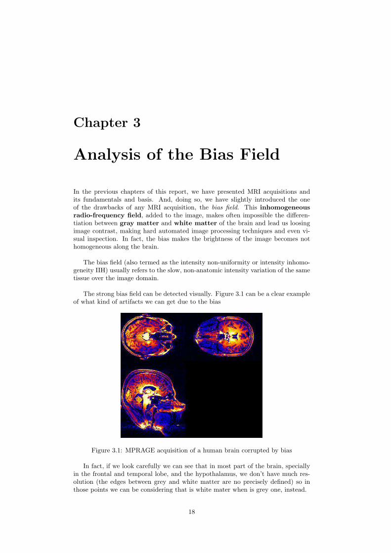
In the previous chapters of this report, we have presented MRI acquisitions andits fundamentals and basis. And, doing so, we have slightly introduced the oneof the drawbacks of any MRI acquisition, the bias field. This inhomogeneousradio-frequency field, added to the image, makes often impossible the differen-tiation between gray matter and white matter of the brain and lead us loosingimage contrast, making hard automated image processing techniques and even vi-sual inspection. In fact, the bias makes the brightness of the image becomes nothomogeneous along the brain.

The bias field (also termed as the intensity non-uniformity or intensity inhomo-geneity IIH) usually refers to the slow, non-anatomic intensity variation of the sametissue over the image domain.

The strong bias field can be detected visually. Figure 3.1 can be a clear exampleof what kind of artifacts we can get due to the bias

Figure 3.1: MPRAGE acquisition of a human brain corrupted by bias

In fact, if we look carefully we can see that in most part of the brain, speciallyin the frontal and temporal lobe, and the hypothalamus, we don’t have much res-olution (the edges between grey and white matter are no precisely defined) so inthose points we can be considering that is white mater when is grey one, instead.

18

Besides, a part from the shifting between gray or white matter, in the imagebe can see bright spots in the center and in the frontal and backwards part of theimage. Is, exactly, in the center of the image where we are supposed to have the bestSignal-to-Noise Ratio but, in 7T acquisitions, this region is the most corruptedby the bias field. Actually, due to this extremely high brightness, we are not ableto discern none of the pixel values on it, and so, we cannot see this regions withenough precision to determine whether some disease or not.

In fact, the presence of IIH can significantly reduce the accuracy of image seg-mentation and registration, hence decreasing the reliability of subsequent quanti-tative measurements. Our main goal is to remove or at least reduce this artifact,giving a nice and clear insight view of all parts of the human brain.

3.1 Mathematical approach for a MR image

The generally accepted assumption on intensity inhomogeneity (for low-field acqui-sitions) is that it manifest itself as a smooth spatially varying function that altersimage intensities that otherwise would be constant for the same tissue type regard-less of its position in the image. In the most simple form, the model assumes thatthe intensity inhomogeneity is multiplicative or additive which means that theintensity inhomogeneity filed multiplies or adds to the image intensities. [36]

Either on what is the source of the inhomogeneity we want to model, we usethe multiplicative form or the additive. Most frequently, the multiplicative modelhas been used as it is more consistent with the inhomogeneities of the receiving coilbut, for modeling the inhomogeneities due to induced currents and non-uniformityexcitation the additive model is more suitable [29].

In addition to intensity inhomogeneities , the MR image formation model shouldinclude the noise, which is supposed to be at high-frequencies. This noise is knownto have a Rician distribution even if, as the Signal-to-Noise ratio (SNR) is not toolow, we can approximate it by a quasi-Gaussian (so, Rayleigh distribution) [28].The next section is entirely devoted to the noise in MR acquisition, so we will focuson it later.

Different models of MR image formation has been proposed in the literature.The most common is the one that assumes an multiplicative bias field and an ad-ditive noise. But, how we get to the signal expression?

The image processing (as we have seen in Chapter 2) begins when all the MRinformation is stored in the k-space. When this space is full, the data is transformedonto the r-space data by simply computing an FFT [30], [23], [13]. Is when applyingthis FFT, when we get the spatial information needed for processing the image. Infact, the two distributions carry exactly the same information (even if the rawdata, the one stored in the k-space, contains the frequency information). Thetransformation from one to the other is, following [30]:

ω(r) =∫

W (k) exp(−2πj(kr))dk. (3.1)

So, after acquiring the signal and translate it into the r-space, this acquired signal

can be expressed as:

s(x) = (o(x) + nbio(x)) ∗ h(x) + b(x) + nRM (x), (3.2)

where:

• s(x) is the measured and digitalized data.1

• x = (x, y, z). (x, y) are the spatial coordinates of each slice and z moves alongthe different slices.

• o(x) is the ideal bias and noise free image.

• nbio(x) is the biological noise due to interior structures of the tissues, physio-logical noise, cardiac rate, respiration motion...

• h(x) is the model of the blurred border region effect due to discrete samplingof the tissue.

• nMRis the noise due to the measuring devices acquisition.

• b(x) is the added bias field (considering its value 0 < b(x) < 1).

Considering how the signal intensity, the noise and the bias field interact, wecan find some easier approximations, which lead us to the same results withoutmaking any assumption about the value of h(x). Even if two sources of noise aredescribed in the signal form (the biological one which corresponds to the withintissue inhomogeneity and the scanner noise that arises from MR devices imperfec-tions), usually only one of this sources is modeled [36].The most common modelassumes that the noise, with a Gaussian distribution, arises exclusively from thescanner and is therefore independent from the bias field. So, following this model,the acquired signal can be approximated as:

s(x) = o(x)b(x) + nRM (x). (3.3)

If we consider that only the biological noise interacts in the image formation, weget another expression for the obtained signal, where the ideal signal o(x) and thenoise nbio(x) are scaled by the intensity inhomogeneity field b(x) so that the SNRis preserved [24].

s(x) = (o(x) + nbio(x))b(x). (3.4)

For images acquired in low-field, we can use, without loss of generality, theequation 3.3 for modeling the received signal. In this case, as we know that in themain part of the image n(x) << o(x) · b(x), we can achieve a good bias removal(as so that, image correction) by dividing the corrupted image s(x) by a correctestimation of the bias field b(x). So that, the corrected image can be expressed as:

o(x) =s(x)

b(x). (3.5)

So, if our approximation for the bias field in good enough to consider b(x) ∼= b(x),then we lead to the result:

o(x) = o(x) +n(x)

b(x). (3.6)

In the parts of the image where n(x) ∼ o(x) · b(x), the signal is not recoverable.

1We must recall at this point the FFT transformation presented in Chapter 2 for image com-putation(see equation 2.27)

The third MR image formation model is based in logarithmic transformed in-tensities, by which the multiplicative inhomogeneity becomes additive. We can seethis last model as the logarithmic version of the multiplicative model. The signalmodeled in this log-transformed intensities model can be written as:

log(s(x)) = log(o(x)) + log(b(x)) + n(x), (3.7)

were the noise is still assumed to be Gaussian, which is methodologically convenientbut inconsistent with the first model 3.27, where the noise is assumed to be Gaussianin the original non-logarithmic domain. Avoiding this fact, the corrected signal willbe:

log(o(x)) = log(s(x))− log(b(x)) ∼= log(o(x) +n(x)

b(x)). (3.8)

If we focus in the noise term of the corrected form, recalling it n′(x) = n(x)b(x) , we

can see that the first factor (n(x)) is a random term with zero mean and constantvariance (in fact we are considering the noise as a Gaussian with zero mean). Thesecond term, b(x) is a deterministic values which varies between 0 and 1 values.This fact lead us to have an strong dependence between the variance of the noise inthe corrected image (n′(x)) and the bias field value at the same point. That is, saythat the noise variance is higher in the points where the bias value tends to zero.This behavior on the variance of the noise is due to the non-uniform Signal-to-Noiseratio along the data set of the acquired image.

3.2 Tissue Signal Distribution

The human brain is mainly composed by three different tissues: grey matter (GM),white matter (WM) and cerebrospinal fluid (CSF). Each of them has different con-centration of water, and so, hydrogen atoms. This uneven number of hydrogenatoms in each element allows different excitations depending on the matter. Thisnucleous, present in water molecules, allow the soft-tissue contrast, specially withthe MPRAGE acquisition protocol, giving different intensity values depending onthe sort of tissue.

In fact, each MR image is modeled in the r-space (see eq.2.27) as a finite com-bination of regions. So for each type of tissue, we get a value of intensity that wemodel it. We assume this intensity distribution as Gaussian function of mean µk

and variance σ2k (see [4]), both are measured in gray levels and k identifies the

different tissues . The probability of an intensity value in a voxel yi, can be written(as long as be are assuming each pixel belong just to one class of matter) as:

P (yi|µk, σ2k) =

1√2πσ2

k

exp(− (yi − µk)2

2σ2k

) (3.9)

that means that for each type of matter in the brain we will have a gaussian in-tensity distribution fitting its brightness, so, in theory, we can to distinguish them.This model is useful for posterior processing techniques, like segmentation of tissues,where we identify the different tissues in the image for its treatment.

Unfortunately, the image not only presents noise, but also Intensity Inhomo-geneity (IIH or bias field). This artifact makes the intensity of a certain voxel shiftfrom its mean value. If this shifting is big enough (and, unfortunately, it uses to be)the intensity value of the voxel can be considered to belong to the another class.In general, IIH artifacts makes the intensity of the pixel of the same tissue vary

significantly, overlapping with pixels of the different tissues.

For study this effects (the one due to the noise and the one due to the bias) wecan compute the image histogram. The histogram of an image shows the relativefrequency of occurrence of levels of gray in an image. That is, h(rk) = number ofpixels with gray level rk.

Let us compare two different histograms:

Figure 3.2: Histogram of brain tissue with IIH. Figure (a) showstwo different histograms obtained from BrainWeb-simulated database page(www.bic.mni.mcgill.ca/brainweb) one with noise and without IIH (solid line) andthe other with noise and IIH (dashed line). Figure (b) is the histogram from a realbrain image.

Figure 3.2(a) clarifies the bias field effects we want to explain. The tissue in-tensities had been modeled as Gaussian functions2(see eq. 3.9). So that, in Figure3.2 we can distinguish the three tissues the brain is composed by. From left toright, the first peak represents the CSF matter, then we find GM and finally WM.When IIH is added to the simulation (dashed line on Figure 3.2), the differentiationbecomes harder, as the IIH makes the amplitudes of the intensities of the tissuessmaller an nearly similar. In fact, noise makes the peaks get wider and IIH dimin-ish its amplitude value. This fact is which lead us to sometimes have wrong tissueclassification.

3.3 The Noise in MRI

The noise, as seen before, is an important factor in our correction, so it will beuseful to give a little insight on it.

The radio-frequency signals observed at the receiver (before they are FFT-transformed to give us a received signal), are corrupted by a noise that we assume

2Notice that we can do that because our intensity signal has noise (recall eq. 2.27) so it givesus some variance that allows us to model it as Gaussian.

to be thermal. This thermal noise is accurately modeled as White and Gaussian-distributed noise. Then, as the received signal, this noise is FFT-transformed ontothe r-space (converting it from the k-space into spatial coordinates), but as theFourier Transform is a linear transform, the noise distribution at the output, stillremains Gaussian.

The problem appears after phase-encoding the signal3. Due to phase encodingerrors, the reconstructed image will be complex, thus, there is white Gaussian noiseon both real and imaginary components of the signal. That is, our noise becomesRician if we take the absolute value of it [26].

The Rician PDF(Probability Density Function) is generated by taking the ab-solute value of two Gaussian random variables with non-zero mean. If we considertwo deterministic measurements corrupted by additive Gaussian noise:

x1 = µ1 + n1, (3.10)

andx2 = µ2 + n2, (3.11)

where n1 ∼ N(0, σ2) and n2 ∼ N(0, σ2). Then x1 and x2 are both Gaussian randomvariables with x1 ∼ N(µ1, σ

2) and x2 ∼ N(µ2, σ2). Therefore, we can define a need

random Rician variable as r =√

x12 + x2

2 with a PDF:

pr(r) =r

σ2exp(−r2 + A2

2σ2)I0(

Ar

σ2), forr > 0. (3.12)

I0 is the zeroth-order modified Bessel function for the first kind:

Io(x) =12π

∫ 2π

0

exp(xcos(θ))dθ, (3.13)

and A = µ1 + µ2

The fact is that, actually, the noise associated with the acquired MR signal isgenerally taken to be additive, uncorrelated and Gaussian with zero (or low valued)mean [40]. So the signal can be modeled as:

sm(k) = s(k) + ε(k), (3.14)

where ε(k) contains the sum over body and electronics contributions.This assumption can be reached by understanding the noise influence in the spatialrepresentation, considering that in the k-space the mean of the noise is zero:

µ(p∆x) =1N

∑

p′ε(p′∆k) exp(j2πp′∆x∆kp) = 0, (3.15)

and its variance:

σ20(p∆x) =

1N2

∑

p′

∑

q′ε(p′∆k)ε(q′∆k) exp(j2πp′∆x(p′∆k − q′∆k)), (3.16)

3Phase-encoding, as we have seen in Chapter 2 (Section 2.3), is the proceeding for encode a 2Dand 3D space in arbitrary coordinate

so it ends as:

σ20(p∆x) =

σ2m

N2

∑

p′

∑

q′δp′q′ exp(j2πp′∆x(p′∆k − q′∆k) =

σ2m

N2. (3.17)

We can extract as a conclusion from here, that we can assume the noise in MRacquisition is an additive single Gaussian distribution. That is to say, the noise isadded to the factor obtained by multiplying the ideal images by the bias.

Regardless of whether the noise is Gaussian or Rician, high noise levels can sig-nificantly decrease the usability of medical imagery. The noise in the complex imagecan be viewed as continuous white Gaussian noise in four dimensions (three spatialand time) [6]. We might maximize the SNR by increasing acquisition time, increas-ing voxel size, increasing coil intensity and applying appropriate edge-preservingfiltering techniques, carefully considering that all this methods have its limitations.

3.4 Bias Field in Low-Field Acquisitions

The MR bias problem occurs in all MR imaging applications. The extent withwhich it occurs and the amount of correction that is needed varies from applicationto application. Intensity Inhomogeneities (IIH) consist in an anatomically irrelevantvariation throughout data generally reflected in a flip angle variation, but triggersin this variation can be multiple. Most tissues have some magnetic susceptibilitywhich can distort the magnetic field; the main magnetic field B0 is not truly homo-geneous in space, and the slope of the gradient-encoding B1is not truly linear (seeChapter 2); the response of the transmitting coil (usually the body coil) is not com-pletely uniform, and for the receiving coil, its response is not homogeneous either;the variations in B0 and B1 can produce location errors rather than intensity errors.

Those are some examples of the artifacts that can affect the image intensity ina MRI but there are some other that can had been grouped has follows:

• Artifacts related to acquisition technique.

– Flip angle variation. One of the parameters set when acquiring the imageis the flip angle4. One image is acquired forcing the hydrogen protonto turn in a certain angle and come back. This angle is the flip angle.The problem is that when increasing the field, this angle value loosehomogeneity all over the brain as not all the spins rotate the same amountof degrees. This flip angle variation is one (let’s us to say the main) causeof B1 inhomogeneities.

– Non-uniform B0 static field. This inhomogeneity can be partially com-pensate by shim tuning. Its main effects is that leads to a partiallydeformation of the imaging plane.

– Gradient fields. The variation in the gradient fields lead to geometricaldistortions.

– RF coil inhomogeneity which depends on its geometry and tuning. Theinhomogeneity is seen in the transmitting coil as well as in the receivingone, but with different dependence with the B1 field.

4When talking about flip angle it refers to the flip angle of the macroscopic magnetizationvector of the RF pulse.(see Chapter 2)

– MR acquisition pulse sequence parameters: repetition time, number ofechoes, interleaved (or not) acquisition.

• Factors linked to the object itself. Tissue-dependent properties as conductiv-ity and dielectric values. Besides, the acquisition protocol takes some minutesto be done, so the normal movements of the patient lead also to inhomo-geneities in the acquired image too.

For a Low-field acquisitions (which means for main fields strengths lower than3 Tesla), the bias field added to the image has been largely studied, so we havesome good approaches for its form or value. In next Chapter we will present theState-of-the-Art of this bias correction methods and its drawbacks when correctingacquisitions at high fields.

3.5 Drawbacks when Increasing Field Strength

Nowadays, the bias field we obtain when acquiring a MRI is nearly assessed whenthe main field applied is not higher than 3T . In fact, as we will see in Chapter 4.1in the low field case, due to its slow and smooth variation, it can be approximate bysome basis smooth functions, as the Legendre Polynomials so the approximation isgood enough to be used to correct the original image from this artifact, even for theinhomogeneities induced by the patient. The complexity of the problem increaseswhen increasing the field applied to the sample, as we start loosing phase coherenceso it appear dielectric effects and those due to the conductivity of the tissues. Thoseeffects make the bias field act not as a smooth function, but as a wave.

As the field increases, the wavelength (λ) of the field decreases, until the pointof make the RF field comparable to, or even less than, the dimension of the humanbody. So, at high frequencies, the RF magnetic field (also called B1 field) inside asample exhibits prominent wave behavior. But, how we can explain this behavior?

As the static strength (B0) increases, the frequency of the RF magnetic field(so B1) increases too and, so that, its wavelength decreases. The wavelength de-creases even further in biological tissues, since many biological samples have highrelative dielectric constants. Due to this decreasing, the wavelength and the sam-ple size become comparable. And so, as the sample dimensions represents a largerpercentage of a wavelength, intermediate and far-fields effects, including wavepropagation, become more important. Actually, the significant interactions of theelectromagnetic waves with the load invalidate the use of quasi-static approxima-tions and require the application of the full wave techniques [32].

In brief, the full-wave solution of Maxwell equations demand is due tothe presence of those intermediate and far field effects as the B1 effect that causesimage inhomogeneity is wave interference [7]. In fact, when the applied main field islower than 3T , the far field approximation is good enough because the intermediateeffects are small enough compared to the far-field ones, so the first ones are denied.But, increasing the main static field applied, those effects are no longer negligible.

Additionally, B1 field and source currents are strongly perturbed by sampleloading. The high dielectric constant of tissue results in generating standing wavesin the object that greatly perturb the effective B1 field. Due to electrical conduc-tivity of the tissue, the induced voltage at high frequencies yield in eddy currents

large enough to attenuate the applied B1 with increasing depth in the body [14].

Besides, the B1 field distribution inside a sample is important for the SpecificAbsorption Rate (SAR). Specific absorption rate (SAR) is a measure of the max-imum rate at which radio frequency (RF) energy is absorbed by the body whenexposed to radio-frequency electromagnetic field. It is used for exposure to fieldsbetween 100kHz and 10GHz [1]. The SAR value will depend heavily on the ge-ometry of the part of the body that is exposed to the RF energy, and on the exactlocation and geometry of the source of the RF energy. Actually, the electrical prop-erties and size of the sample strongly affect the RF field distribution (in magnitudeas well as polarization) at high field strengths.

The polarization of the RF field inside the sample varies drastically such thatthe RF field in certain regions can rotate predominantly in the direction oppositeto the direction intended in driving the coil.

So, in resume, any mathematical approach of RF field inside the sample (and inour case, inside the brain) can be extremely complicated due to:

• The quasi-static approximations of Maxwell’s equations are not valid. A fullversion of Maxwell’s equations must be employed.

• Human body geometry is irregular and it has different conductivity and di-electric rates (specially in air-tissue boundaries).

Talking about brain imaging, non uniformity image intensity at high field isprominent and frequently observed when the human head images are acquired witha volume coil. It is reflected as a hyperintense region in the center of the head (seeFig. 5.1) and can be considered to be due to the partially-constructive superpositionof RF waves transmitted from each of the conductors in the coil and reflected fromthe sample boundaries, plus the still-substantial near-field contributions. Artifactsdue to wave behavior are initially observed at 3T and become more prominent inimages acquired at higher field strength.

In resume, when imaging using MRI techniques, as frequency increases, elec-tromagnetic waves decay faster in the brain (as human brain tissues are neitherpurely dielectric nor purely conductive) and the boundary between brain and airbecomes less reflective. So that, the amplitude distribution of the fields in the headis the result of the interference pattern of decaying traveling magnetic waves ina given sample-coil configuration plus contribution from near fields. Besides, andno less important, electromagnetic properties of grey and white matter for humanbrains are inverse: conductivity increases while dielectric constant decreases withfrequency, which means that the bias field is different in both.

Arguably, the major problem of these 7T images acquisitions is that we cannot make the assumption that the bias has a smooth variation anymore. And this,unfortunately, is almost the only supposition used in almost all kinds of retrospectivemethods for bias correction and/or compensation in human brain imaging.5

5Retrospective methods are postprocessing methods that propose to correct MR images withonly few assumptions on the acquisition process. In Chapter 4.1 we will make an overview of someof those methods.

(a)

Figure 3.3: Hyper-intense region in the center of the head at 7T and its 3D view .

3.6 Bias Field in High-Field Acquisitions

As seen above, RF behavior becomes complex at ultra-high magnetic fields. Abright center and weak periphery are observed in images obtained with volumecoils. Destructive interferences are responsible for this variations of brightness inthe image [37]. But, how we can model the signal intensity in such acquisitions?

In paper [16] a study for the polarization of B1 field over a water phantom isperformed. It would give us an insight of wave behavior we want to model in 7Tacquisitions. Following its wave behavior and after considering full-solution Maxwellequations, the transmitted field can be decompose into two rotating components:

B+t =

(Btx + iBty)2

B−t =

(B∗tx − iB∗

ty)2

. (3.18)

Where the absolute value of the polarization component |B+t | is given by:

|B+t | = ([Re(B+

t )]2 + [Im(B+t )]2)

12 . (3.19)

The calculation for the receiving field is similar. The reception field Br can also bedecomposed in two circularly components:

B+r =

(Brx + iBry)2

(3.20)

B−r =

(B∗rx − iB∗

ry)2

. (3.21)

where|B+

r | = ([Re(B−r )]2 + [Im(B−

r )]2)12 . (3.22)

The transmission and reception fields are two physically different fields, so theymust be calculated separately for producing the image intensity distributions. Actu-ally, the polarization behavior of RF field plays an important part in the formationof the image intensity distribution in a human sample at high field. The transmis-sion field is produced by the input current in the coil and the reception one by thecurrent induced by the transverse magnetization. This leads the transmission field

rotate in the same direction as the magnetization precession whereas the receptionfield rotates in the opposite direction. The later one is used when the principle ofreciprocity is applied for evaluation of the reception distribution.

In figure 3.4(a), the plot for |Bt| shows the field strength distribution, while|Bt

+| and |Bt−| depict the positive and negative circularly polarized components

of the transmission field. The βt contour plot (shown in figure 3.4(b)) describesthe polarization distribution of RF field without the implication of the spatial fieldstrength variation.6 [37].

Figure 3.4: Grayscale plots of the transmission field and its circularly polarizedcomponents (a), and the contour plot of βt (b) of the quadrature surface coil infree space (σ = 0, εr = 1). This plot is a ratio of the transmission field defined asβt ≡ |B+

t ||B+

t |+|B−t |Image obtained from paper [16]

The overall intensity of |B+t | is significantly stronger than |B−

t |, whereas |B−r | is

much stronger than |B+r |. So, from here, we can assess that the direct responsible

for the MR image intensity distribution are on one hand B1 field, and on the otherhand its circularly (actually elliptical) polarized components B+

t and B−r . So, from

this moment, we will consider B+1 = B+

t and B−1 = B−

r .

In resume, the RF field interacts with magnetization through the circularlypolarized components, which can be constructed on an axial plane through thecenter of the sample as:

B+1 =

(Bx + iBy)2

B−1 =

(Bx − iBy)2

, (3.23)

assuming that B+1 is in the direction of nuclear precession, so that, is the component

that determines the excitation.

6The nuclear spin precession is assumed to be in the positive (counterclockwise) direction.

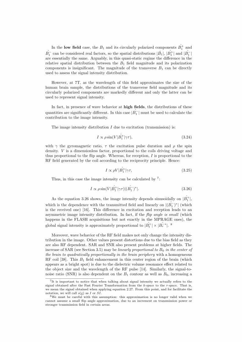
In the low field case, the B1 and its circularly polarized components B+1 and

B−1 can be considered real factors, so the spatial distributions |B1|, |B+

1 | and |B−1 |

are essentially the same. Arguably, in this quasi-static regime the difference in therelative spatial distribution between the B1 field magnitude and its polarizationcomponents is insignificant. The magnitude of the transverse B1 can be directlyused to assess the signal intensity distribution.

However, at 7T, as the wavelength of this field approximates the size of thehuman brain sample, the distributions of the transverse field magnitude and itscircularly polarized components are markedly different and only the latter can beused to represent signal intensity.

In fact, in presence of wave behavior at high fields, the distributions of thesequantities are significantly different. In this case |B−

1 | must be used to calculate thecontribution to the image intensity.

The image intensity distribution I due to excitation (transmission) is:

I ∝ ρ sin(V |B+1 |γτ), (3.24)

with γ the gyromagnetic ratio, τ the excitation pulse duration and ρ the spindensity. V is a dimensionless factor, proportional to the coils driving voltage andthus proportional to the flip angle. Whereas, for reception, I is proportional to theRF field generated by the coil according to the reciprocity principle. Hence:

I ∝ ρV |B+1 |γτ, (3.25)

Thus, in this case the image intensity can be calculated by 7:

I ∝ ρ sin(V |B+1 |γτ)|(B−

1 )∗|. (3.26)

As the equation 3.26 shows, the image intensity depends sinusoidally on |B+1 |,

which is the dependence with the transmitted field and linearly on |(B−1 )∗| (which

is the received one) [16]. This difference in excitation and reception leads to anasymmetric image intensity distribution. In fact, if the flip angle is small (whichhappens in the FLASH acquisitions but not exactly in the MPRAGE ones), theglobal signal intensity is approximately proportional to |B+

t | × | ˆB−∗r |. 8

Moreover, wave behavior of the RF field makes not only change the intensity dis-tribution in the image. Other values present distortions due to the bias field as theyare also RF dependent. SAR and SNR also present problems at higher fields. Theincrease of SAR (see Section 3.5) may be linearly proportional to B0 in the center ofthe brain to quadratically proportionally in the brain periphery with a homogeneousRF coil [38]. This B1 field enhancement in this center region of the brain (whichappears as a bright spot) is due to the dielectric volume resonance effect related tothe object size and the wavelength of the RF pulse [14]. Similarly, the signal-to-noise ratio (SNR) is also dependent on the B1 contour as well as B0, increasing a

7It is important to notice that when talking about signal intensity we actually refers to thesignal obtained after the Fast Fourier Transformation from the k-space to the r-space. That is,we mean the signal obtained when applying equation 2.27. From this point, and for facilitate thenotation, we will call s(x) as I or SI.

8We must be careful with this assumption: this approximation is no longer valid when wecannot assume a small flip angle approximation, due to an increment on transmission power orstronger transmission field in certain areas.

better than linear proportion in the brain center and at less than linear rate in thebrain periphery when a homogeneous coil is used. In brief, SAR and SNR as wellas image inhomogeneity and contrast vary with the B1 contours in the anatomy [38].

3.7 Summary of Analysis of Bias Field

In this chapter we have presented an approximation for the bias field in MR ac-quisitions, and for the noise added in the images. This approximation is neededin order to find methods to compensate it and give a clear image of the tissues wewant to study.

The general model for the signal intensity presuppose, without lost of generality,an multiplicative bias field and an additive white gaussian noise. That is:

s(x) = o(x)b(x) + nRM (x). (3.27)

For low-fields acquisitions (which includes the acquisitions performed withfields lower than 3T ), the IIH manifest itself as a smooth spatially variation and ithas been modeled by fitting its shape with smooth functions. Otherwise, we haveseen that when increasing the main field value, this assumption is no longer feasible.

For high-field acquisition, the bias field acts as a standing wave so the full-wave solution of Maxwell equations is needed. As frequency increases, the wave-length decays faster and the boundaries between tissues become less reflective andthis leads on contrast lost between tissues. The amplitude distribution of the mag-netic field is the result of the interference pattern of decaying traveling waves plusthe contribution of near-field effects.

So that, any mathematical approach of the RF field inside the sample can becomplicate. The methods for bias compensation in this case must take into accountother factors, as we will see in next Chapters.

The main contribution of this master thesis is demonstrate that, due to thiswave behavior, the bias field corrections performed until now are not enough forcorrecting 7T acquisitions. All the conclusions an results we will shown in posteriorChapters are based in the fact that at 7T the bias can not be assumed as a slow andsmooth variation. This report focus in MRI acquisition of human brains images, butactually, the bias appears in all MR imaging techniques, whereas we are imagingthe brain or other parts of the body. So that, the conclusion we will assess for thespecific case of the brain, can be extrapolate to other MR images.

Chapter 4

State-of-the-Art Methods forBias Correction

Since the apparition of the MR techniques for imaging human body, automatedanalysis had become mandatory to efficiently cope with the large amount of datagenerated using them. Besides, several artifacts affect the quality of the data, witha considerable amount of degradation. Huge efforts had been placed on findingmethods to erase (or at least compensate) the bias field from the image. In fact,the goal of all this methods is to facilitate all the quantitative and qualitative anal-ysis of this data, like segmentation or registration protocols.

This Chapter is an overview of the most important methods proposed in therecent literature. We will enumerate some of them and, after that, we will focuson specific ones, validating them for our specific purpose: bias correction in 7Tacquisitions.

4.1 Prospective and Retrospective Methods

Intensity non uniformity (IIH) has different sources. Actually, such artifact that canaffect the image intensity can be related (1) to the acquisition technique, as theycan be induced by the coils used in the acquisition protocol, the sequence selectedor related to (2) the nature and the geometry of the sample, as RF penetration orRF standing wave effects, otherwise [5]. Considering this rough division, we canassume two different parts in the MRI correction process, sorting all the existingmethods according their location in the acquisition/processing pipeline and on theassumptions those methods rely on. We can define:

• Prospective methods, focused on the acquisition part which is, let us tosay, the ”physics’” part.

• Retrospective methods, that rely on the post-processing part, so wecan consider them to belong to the signal processing methods.

For the first ones, their goal is to improve the acquired image quality by a bet-ter acquisition protocol. Image processing community, instead, try to improve thisquality by the use of retrospective algorithms as first steps to improve quantitativeanalysis. This is a rough classification of the correction/compensation methods forbias in MR acquisitions, as most of them rely in different assumptions.

31

4.1.1 Prospective Methods

Prospective methods are based on prior knowledge about acquisitions parameters.If we recall the signal model seen in Chapter 2 (equation 3.3)

s(x) = o(x)b(x) + nRM (x), (4.1)

we notice we have an ill-posed problem: neither the bias, b(x), nor the true intensityspatial distribution, o(x), are known. But, we can get a prior knowledge of themby using specially designed MR acquisition protocol.

These methods suppose the IIH due to the combined effect of (1) the sample,(2) the MR pulse sequence and (3) the coils, so to get knowledge of one (or more)of this parameters can facilitate the way for bias correction. That is, prospectivemethods try to reduce the number of unknown factors involved. We can find twomain different approaches to this purpose:

1. Combine different data sets.

2. Trying to compensate unwanted flip angle variation during the acquisitionprocess.

Different data sets combination

There are several ways to get multiple data set combinations. One first approachis to acquire images from different objects (usually phantoms) with the same imag-ing parameters [5]. In this case we will be considering data sets only affected bysequence-dependent and coil-dependent components of IIH. So, once the parametersare set, the IIH will be directly related to the coil sensitivity. This gives a good rep-resentation of the receiving coil sensitivity variation [3]. The main limitation is thatthis approach does not take into account the influence of the imaged object. Andas we have seen in Section 2.6, this effects can be really important when increasingthe main field strength. So that, those methods are not valid for bias correction at7T MR imaging.

Other methods face the problem from another point of view: they acquire datasets of the same object changing the imaging parameters. In this case, they tryto remove the IIH component due to the object studied. In fact, they get a prioriknowledge of the bias field added by using different acquisition protocols or differentcoils [5].

Liney et al., in 1998 [22], use same coil acquisitions with different imaging pa-rameters, considering that an homogeneous tissue is modeled by an homogeneousintensity distribution (see Chapter 3.1, section 3.2, equation 3.9)

P (yi|µk, σ2k) =

1√2πσ2

k

exp(− (yi − µk)2

2σ2k

). (4.2)

In this case, any variation in signal intensity is attributed to the bias field. So, theyconsider the corrupted data as a representation of the bias field spatial variation.They assessed that a T2-weighted sequence can be corrected using the bias estima-tion obtained from a PD-weighted (proton density) sequence.

In all this cases, the correction is not complete, as they are only focusing inone of the sources of the bias. In low-field case, the bias is not as strong as theone we get when working at high-fields strengths. Is for that reason, that those

methods, even if they just focus in one origin of the IIH, work in a acceptable wayin low-field acquisitions but not as good as we want in high-fields. So, and withoutdenying them, we can assess that those prospective methods are not suitable forour purpose: bias correction in 7T acquisitions.

Instead of acquiring different set using the same coil but changing image param-eters, we can fix this parameters and acquire the data set changing the receptionand transmission coils. Surface coils have good SNR but really poor uniformity,while body/volume coils are assumed to have uniform sensitivity. A pre-scan of lo-calization data can also be performed, to obtain prior knowledge about the bias field.

Flip angle variations compensation

A part of the multiple set combination, prospection methods with pre-acquisitionflip angle compensation had been performed too. Actually, as we will see in Chapter??, in this master thesis we propose a method which combine the acquisition of aflip angle map with some post-processing techniques applied to the acquired imageto perform its correction.

Coming back to our topic, this second group of prospective methods, assume theIIH mainly due to the RF coil, so they first estimate the sensitivity for a particularhead coil along the z axis. Then they compute a Look-up-table (LUT) to correctthe variations based on the estimate sensitivity profile [8].

Deichmann et al., in [11] designed an specific RF excitation pulse, based on twospatially independent terms, compensating unwanted flip angle variations in a headcoil. Actually, this master thesis will give lay in this method, giving a differentapproach from the one assess by Deichmann (that will be in Chapter ??). We willpropose (see Chapter ??) the use of a flip angle map (also called RF map or B1 map)for determine the bias in the acquisition. In that way, and using post-processingmethods (id est, a retrospective method), we will try to correct the bias in the MRacquisition.

In fact, the main goal of this thesis is to give a bridge between the prospectivemethods and the retrospective ones. Instead of focusing in compensate the bias fieldacting only in one of the, let’s say, segments of the acquisition/processing protocol,we will try to combine techniques applied in both of them.

The main idea is that we can combine the knowledge obtained from both seg-ments. That is, if the methods proposed at this moment are not god enough forachieving the correction, why don’t combine two of them, to get better results?

4.1.2 Retrospective Methods

Retrospective methods propose to correct MR images corrected by IIH artifact withonly few assumptions regarding the acquisition process. We will focus on them as,from the point of view of signal processing, they are capable to compensate the biasin a more generic way than the prospective methods do.

They can be classified in grayscale level-based or transform domain based meth-ods.

Graysacle Level Based Algorithms

The grayscale level based algorithms rely on the assumption that the bias hassmooth spatially and slow varying across the image , so the ideal image becomespiecewise constant [5]. Different approaches had been mainly developed, focusingeither on assumption concerning the artefact or the true image:

Surface fitting: Is a type of interpolation. Its aim is to fit a set of data pointsto provide a good approximation of the brightness function of the image. Correctionis performed dividing voxel-by-voxel the original image by the computed surfacesfollowing the principle shown in Chapter 3.1, in equation 3.6. Depending on thetype of the basis function used, we can found different solutions.

Polynomial Basis Functions: Styner et al., in [31], propose a Parametric BiasCorrection for MR images. It is a multiple pass basis function fitting. Consideringthe assumption of smooth and low variation of the bias, they estimate it by Legen-dre Polynomial, computing its coefficients by minimizing and energy function. Insection 5.1 we will talk about it in a broad way.

Spliline Basis Functions: Those methods fit the basis function by single passfitting or multiple pass fitting.

Spatial filtering: The main assumption of this methods is that the bias is alow spatial frequency intensity variation. So, the methods based in spatial filtering,first extract the IIH, and then perform the correction by dividing the original im-age by the extracted IIH. This spatial filtering is has been generally done with twodifferent kind of filters: the Low-Pass filter and the Homomorphic filter.

Low-pass filtering techniques are normally based on Median filter as it is usefulfor removing outliers (estreme pixels/voxels values). It uses sliding-neighborhoods,ordering the pixel/voxel values in a neighborhood prior to choose the median valueas a result.

Homomorphic filtering is a non-linear filtering technique for image enhancementor correction. This filtering methods rely on the fact that The Fourier transformis linear and associative under addition, but is not associative under multiplica-tion. Thus, Fourier methods are suitable for removing noise from images only whenthe noise can be modeled as an additive term to the original image. In generalimage signal processing, when the noise is not additive, we can define an objectin terms of the illuminance and reflectance so, an image of the object might bemodeled as f(x, y) = i(x, y)r(x, y). According to this approach, input signal isassumed to consist of two multiplicative components: background and details. Illu-mination and reflectance are not separable, but their approximate locations in thefrequency domain may be located. Illumination variations can be thought of as amultiplicative noise, and can be reduced by filtering in the log domain. To make theillumination of an image more even, the high-frequency components are increasedand low-frequency components are decreased.

If we consider equation 3.27, we realize that for an MR image, the bias (b(x)),which is the artifact we want to remove, multiplies our ’ideal image’ (o(x)), so is di-rect to identify ”reflectance” and ”illumination” as ”image” and ”bias”. So, ideally,Homomorphic filtering is supposed to diminish the bias contribution in the image.

Statistical methods: Those methods mainly aim at segmentation, but they

take IIH into account as it is a important factor that can distort segmentationresults. It can be achieved by means of Maximum-Likelihood (ML) and Maximum-a-Posteriori Methods (MAP)-based methods or by Fuzzy-C-Means-based methods.The first two, label pixels according to probability values, which are determinedbased on the intensity distribution of the image. It is an estimation problem thatcan be based in different criteria as MAP or ML. Parameters estimation can beachieve by EM (Expectation-Maximization) algorithm. The expectation step isequivalent to compute the posterior tissue class probability (see. Section 3.2) whenthe bias field is known while the maximization step is equivalent to a MAP estima-tor [5].

The Fuzzy-C-Means-based methods clusters data by computing a measure mem-bership, called the fuzzy membership, at each voxel for specified number of classes.However, FCM is not appropriate for data corrupted by IIH [5].

Transformed Domain Based Methods

All the graylevel-based methods work in the spatial domain, but they also work inother domains as the Fourier or wavelet domain (which are dual), or in the comple-mentary domain of probability density functions (PDF). Some methods had madethis change of domain, as they can make different assumption on the bias.

When computing the PDF, the original intensity spatial distribution becomesintensity probability distribution that we can model as an histogram. In this casethe IIH is considered as a parasitic convolution term which increase entropy. Theidea of those methods is to minimize this entropy and deconvolute the parasiticterm to correct the image [39].

Working on Fourier Transform domain has been seldom used in IIH correction.In fact, normally, the filtering is done in spatial domain (as we have seen in theprevious subsection).

Recently, the used of Discrete Wavelet Transform have been proposed. In [21],Lin et al., use the DWT to decompose the image into a cascade of orthogonal ap-proximation and detail subspaces for different spatial resolutions. Each approximatesubspace contains low-frequency information whereas the corresponding detail sub-space contains high-frequency information. the information of those to subspacescan be combined to achieve IIH correction.

4.2 Summary of State-of-the-Art Methods for BiasCorrection

Since the apparition of the MR imaging techniques, the main goal has been toachieve good soft tissue imaging, developing methods to enhance contrast and reso-lution. In this Chapter we have presented a resume of the State-of-the-Art methodsfor this achievement, methods for bias correction

We cannot forget that MR imaging techniques are in constant development. MRhas always been moving to ever higher magnetic field strength. In point of fact,increasing the main field strength allow us to get advantage of a better signal-to-noise ratio (which increases almost linearly with the field strength [27]). Thisimprovement of the SNR allows higher spatial resolution and/or faster imaging,

a greater spectral dispersion, as well as an enhanced sensitivity to magnetic sus-ceptibility. But, if we increase the field, we find unsuitable effects or artifacts thatcannot be treated as we have been doing with low-field acquisitions. And this factbecomes a problem.

Actually, all this methods are plenty proved in low field acquisitions. Theyare based in the assumption of smooth and slow variation of the bias field alongthe image. Unfortunately, as we have seen in Chapter 3.1, for high field strengthsthese assumptions are no longer correct. That means, the methods are no longersuitable for our purpose: bias correction in 7T MRI acquisitions. In next Chapterwe will present some studies about two of the grayscale based methods, showing itsdrawbacks in the correction at high fields. The PABIC (Parametric Bias Correctic)and the LPF (low-pass filtering) approachs are studied, and analyzed. In Chapter??, a new method is presented, a method which try to palliate this deficiencies.

Chapter 5

Analysis of RetrospectiveMethods

In the Chapter 4, we have presented the State-of-the-Art methods used nowadaysfor bias correction, sorting them in two different categories: prospective and ret-rospective methods. The idea is to show that, even thought those methods havebeen largely tested in low-field MR acquisitions, they become weak for correct im-ages acquired at higher fields. That is, the main drawback of this methods appearswhen we increase the main field strength as they have not demonstrate to be ableto correct the image IIH due to RF field inhomogeneities.

In this Chapter we will study the two mainly used methods for correction ofMR images, proving its unsuitability for achieve IIH correction in MR acquisitionof over 7T . The PABIC and the Low-Pass filtering approaches are studied. Ourgoal is to achieve a common brightness level for each tissue in the image. The quan-titative analysis will be performed in terms of the Mean Square Error (MSE)between the corrected image and the image assumed as Ground Truth and the timeelapsed in the simulations. Notice that the power of the computer is responsible ofthe time elapsed when running the correction. The tests had been performed overa Intel(R) Core(TM)Duo CPU 6600 @2.40GHz, 1.98GB of RAM.

We should clarify that, when talking about 7T MR acquisitions, it is difficultto assess the quality of the correction as we only deal with corrupted data, so eventhe ground truth used for the comparison present some bias corruption.

5.1 The Parametric Bias Correction (PABIC)

As seen before, the PABIC is a retrospective method for IIH correction mainlydeveloped by Martin Styner from University of North Carolina. This polynomialapproach combines bias correction with histogram adjustment. It is not only fo-cused in bias correction. In fact, besides the correction of intensity inhomogeneitiesin magnetic resonance imaging (MRI) it significantly improves intensity-based tis-sue segmentation. Actually, at the same time as the bias correction, and to facilitateit, PABIC runs a tissue segmentation of the image, with the estimation of meanand variance values assess for each tissue by the user.

PABIC is based on a simplified model of the imaging process: a parametricmodel of tissue class statistics, and a polynomial model of the inhomogeneity field.The authors [31] assume that the image is composed of pixels assigned to a small

37

number of categories with a priori known statistics. Further they assume that theimage is corrupted by noise and a low-frequency inhomogeneity field. The esti-mation of the parametric bias field is formulated as a nonlinear energy minimizationproblem using an evolution strategy (ES). The resulting bias field is independent ofthe image region configurations and thus overcomes limitations of methods basedon homomorphic filtering. Furthermore, PABIC can correct bias distortions muchlarger than the image contrast.

The main idea of this method is to determine the correct class k which eachpixel/voxel belongs to, in order to obtain an intensity-based segmentation of theimage. As we have presented in Chapter 3.1, human brain have three main classesof tissues: white matter (WM), gray matter (GM) and cerebrospinal fluid (CSF),thus, in this case, k = (1, 2, 3). Here, we must make a consideration. Human brain,a part from this three types of matter, is composed by other classes such as skull,skin, blood vessels... This classes are considered to be too small and morphologi-cally complex to help in the correction so, in a previous step, they are removed bypre-processing protocols as skull-stripping and masking. We will talk about themlater.

The Parametric Bias Field Correction (PABIC) relies, in one hand, on the modelof the image intensity presented in Section 3.2 and, in the other, on the fact thatb(x) can be thought as a combination of m smooth basis functions (which are Leg-endre Polynomials). In this method, b(x) is modeled as b′(x, p), where x are thespatial coordinates and p the coefficients of the Legendre Polynomials.

The p parameters are estimate directly from data by the iteratively search of theglobal minimum of a energy function, stepping-out from non-optimal minimum [31].This energy function is:

e(p) =∑

i

(ui − vi(p))2, (5.1)

where ui is the data and vi(p) is model a used to parameterize single-class modeland is found between Valley functions which is a robust family of M-estimators:

valley(d) =d

d2 + 3σ2, (5.2)

showing inflection points at d± σ. The valley functions of each class are multipliedso the total energy function remains:

etotimage(p) =∑

xεimage

Πkvalley(s(x)− b(x, p)− µk). (5.3)

We must know that finding p(x) by minimizing this energy function is a nonlinearproblem. The method used in PABIC for this minimization is the 1+1ES algorithm,where each p(x) represent an individual. Its operation is shown in Appendix E.

PABIC rely in some assumptions:

• The bias field (b(x)) has slow and smooth variation and its mainly due to theRF field and partially induced by the patient.

• The bias field (b(x)) can be approximate by a parametric model b(x, p) as asuperposition of Legendre Polynomials.

• The intensity of the signal for a given class is modeled as a Gaussian of meanµk and variance σ2

k.

• The hypothetical idealized signal (o(x)) consists on pixels/voxels x each ofwhich can be assigned to a unique tissue class.

• Noise (n(x)) is caused by biological tissues.

This method is fully automatized, and prior to its application to a specific imagesome parameters must be set. This parameters are divided in three groups: (1)parameters for the class model, (2) parameters for the bias field model and (3)parameters modeling the optimization. They are listed below:

1. Class parameters:

• Number of classes

• Mean and variance values for each class

• Class mask

2. Bias estimation parameters:

• Type of bias field

• Order of Legendre Polynomials

3. Optimization parameters:

• Mutation factors cgrow and cshrink

• Maximum number of iterations

• Initial values of coefficients p

5.2 Results and validation of PABIC Method

To test PABIC reliability in bias correction over 7T acquisitions, several test overan MPRAGE acquisition had been performed, treating the PABIC algorithm as a”black box”. We have used the utility MRI Bias Correction, developed by MartinStyner, from the ITK C++ library [15]. ITK is a cross-platform application de-velopment framework, widely used for the development of image segmentation andimage registration programs. ITK was developed with funding from the NationalLibrary of Medicine (U.S.) as an open resource of algorithms for analyzing the im-ages of the Visible Human Project. ITK stands for The Insight Segmentation andRegistration Toolkit. The toolkit provides leading-edge segmentation and registra-tion algorithms in two, three, and more dimensions.

As said in the previous section, some parameters must be set before runningBias Correction utility. The class parameters must be set, as well as bias esti-mation parameters. Optimization parameters are not compulsory, so in this firstattempt we denied them, working with the default ones.

The choice of the mean and the variance values of each class is not trivial. Infact, PABIC set values for those variables are mainly used to distinguish betweenthe different tissues in the segmentation process which is done parallel to the biascorrection. Thus, it is important to assess them in the most accurate way, to avoidwrong results in the process. For this purpose, we compute the histogram of thetest image and try to accurately discern all the classes considering the peaks in thehistogram.

The first tests were performed with a single slice of an high contrast acquisitionof a human brain at 7T (see Fig.5.1)

(a) (b)

Figure 5.1: 2D human brain image used for first test in bias correction with PABIC.Single slice for a 7T MPRAGE acquisition corrupted by noise and bias (a) and plotof the computed histogram of its axial view (b).

In order to improve the results, we mask the image. This lead us to avoid theparts of the image that are not useful for bias estimation, such as the background.In fact, removing the background allow us to get better results even in computa-tion time, as we are dealing with less information. Both, original and mask imagesmust have the same size. The mask will be superposed over the original image,determining the pixels of this image that will be dismissed. PABIC can also use adefault mask (in case the user does not introduce its own costumed mask). Thisdefault mask is automatically computed by setting to zero value the pixels whichgray level is bellow the 10 per cent of the histogram.

Masking is normally the first step performed in almost all the image processingprotocols. Its utility is to separate the useful data from the noisy background, re-moving this last one. It lays on the hypothesis that the background is the darknesspart of the image, and so that, with the lower gray value in our scale1. So that,the simplest way to compute a mask is by simply threshold the graylevel values inthe image, denying the pixel whom value is smaller than this threshold. There, wewill have a binary image2 so we can multiply it with our image and take only thevalues inside the mask. Figure 5.2 shows the mask used for correcting a 2D slice:

5.2.1 Correcting a 2D Human Brain Image

For testing the goodness of PABIC some features are used. We used the p-vectorand the time elapsed in the simulations. Remember that each p-vector can be rep-resented in a m-dimensional Euclidean space, so we use this output to comparedifferent simulation, taking advantage of some Euclidean operators such as the dis-tance between them and the ground-truth.

The first test performed, was to run consecutive simulations of the same datawith the same conditions but changing the variance of the filter before the masking3.

1Actually, images in standard formats are stored so that each pixel/voxel value lies in a range[0..255]. This range is chosen so that each pixel/voxel can be represented by 8 bits (one byte). So,in this scale, 0 stands for black, 128 for gray and 255 will represent white.

2Binary image is an special kind of intensity image. Contains only 2 levels, 0 for black and 1for white.

3In fact, before masking the image, is usual to low-pass filter it to erase part of the noise. Inthis case, the filtering had been done by changing the variance of the filter, with a fixed window

(a) (b)

Figure 5.2: 2D human brain image used for first test in bias correction with PABIC.Single slice for a 7T MPRAGE acquisition corrupted by noise and bias (a) and themask used for avoiding background (b).

We set the parameters of PABIC as follows: grade m = 3 for Legendre polynomialsand maximum number of iterations 200000 with a personal mask. For this case, wetook as class-means the values µ1 = 129 and µ2 = 198. And for the class-sigma,σ1 = 22 and σ2 = 12. In figure 5.3, the evolution of the computing time is repre-sented.

Figure 5.3: Evolution of the elapsed time in simulation while changing pre-filtervariance

As we see in the image, the mean time elapsed is about 14 minutes. This time is notextremely big, otherwise the correction performed by PABIC is not good. In fact, ifwe take a look to the correction and its vertical and horizontal profiles, we realizedthe are not enough homogeneous, that is to say, the intensity is not uniform alongthe brain (see Figure 5.4). As an additional point, notice that the vertical profilehas a greater slope than the horizontal one. This is because the vertical section is

size

parallel to the surface coil direction4

(a) (b) (c)

Figure 5.4: 2D human brain image corrected with PABIC (a) and its grayscaleprofiles. Horizontal profile (b) and vertical profile (c).

Due to the bad results obtained in our first test, a second experiment was per-formed. In this case, we tried to improve the correction of a 2D acquisition bychanging the value of the maximum number of iterations allowed. In this case,we run PABIC with the same mean and variance parameters, and with m = 3 asthe degree of the Legendre polynomials. Here, a computation of the evolution ofthe Mean Square Error between the p-vectors was performed. For this purpose weaveraged all the p-vectors obtained after the simulation get stable. The modulusof our averaged vector (our ground-truth) is represented in by the red line. Thenumber of iterations varies from 200 iterations until to 4000 by steps of 200. Theresults are displayed in figure 5.5:

Figure 5.5: Evolution of the p-vectors while increasing the number of maximumiterations allowed.

In this figure, we see that when increasing the number of iterations permitted,the Minimum Square Error (MSE) also increases. The increasing is nearly linearwith the number of iterations until 1600 but then it reaches a nearly constant value.That means there is an internal criterion in PABIC which stop the simulation when

4The imaginary line in wich the surface coil is transmitting and receiving signal.

it reaches an acceptable result, even if the number maximum of iterations has notbeen reached. Nevertheless, we notice the result is not acceptable neither. In fact,PABIC stop running the simulation, because the result obtained is the best it canachieve (even if it is not good).

However, we can suppose that the bad results obtained in our second trial aredue to the fact that PABIC is working in a transitory regime. ”Transitory regime”because with this low number of iteration, PABIC demonstrate to not be able toreach a global minimum of the energy function, but a local one instead. Keepingthe same parameters, we tried to improve the MSE by increasing the number ofiterations allowed. We start computing the correction up to 40000 iterations. Theresults are displayed in the next Figure.

(a)

(b)

Figure 5.6: 2D human brain image corrected with PABIC (a) and the evolution ofthe p-vectors while increasing the number of iterations up to 40000 (b).

We notice, the MSE had been improved (avoiding the aberrant measures ob-

tained for 150000 and 300000 iterations). Nevertheless, the correction is not goodenough as we can see in the Figure 5.7 (a). The intensity all over the tissues is nothomogeneous, so we cannot say PABIC is correcting it.

At this point, we get really sceptical about if PABIC is capable to correct an7T MRI acquisition. As said in Chapter 3.1, the bias is assumed to be smooth andslow variant when the magnetic field applied in the acquisition is lower than 3T ,but it does not behave in this way in high-field acquisitions. PABIC lays in thisassumption, so it performs pretty good bias corrections in low-field acquisitions butnot in higher fields. However, some other test had been performed. In this case,with a 3D image.

5.2.2 Correcting a 3D Human Brain Image

As seen in Chapter 4.1, PABIC presents other abilities. It is capable to correct thebias field in the 3D space5 for acquisitions under 3T , so we try to test the methodworking full power fot 7T acquisitions.

A 3D MRI acquisition is a group of different 2D correlative slices . In our case,the correction was performed over a 3D volume consistent in 128 slices of 192x192pixels per slice.

We have to notice, that working over a 3D image will increase the computationtime. Actually, we have N slices of 192x192 so the time will be increase by thisfactor, where N is the number of slices.

For achieve this corrections, the same parameters were set in PABIC utility,allowing until 500000 iterations. The class-means and the class-sigma remained thesame as the case of 2D correction. In this case, the time elapsed in simulation was40 minutes, but the correction was not good. As we can see in Figure 5.7, whereone single slide is shown:

(a) (b)

Figure 5.7: Slice of a 3D volume human brain image corrected with PABIC (a) andits intensity histogram (b).

The image is still corrupted by bias and the histogram shows the imperfect correc-tion. The three main classes are not discernible as the maximum values of eachgaussian are nearly the same, even if they represent three different kinds of matter.

5Remember that an MRI acquisition translated into the r-space is corrupted in all directions.

To plot the vertical and the horizontal profile lead us to clarify this aspect. Infigure 5.8, these plots are represented. In fact, here we see the shape of the profilesare specially variant. This let us assess that the bias field in a 7T acquisition has notany smooth variation. Besides, bias affected the image much more than noise (evenif we can see the noise artifact if the take a look at higher frequencies). Besides, wecan realize, looking at the vertical section that the maximum of the image is notexactly situated in the border of the image but a little bit further than that. Thisfact will lead us to have a high frequency discontinuity in the image, and is showing(again) that we do not have smooth variation of signal intensity, but a higher one,otherwise.

(a) (b)

Figure 5.8: Vertical (a) and horizontal (b) profiles of gray values of one slice ofa 3D human brain acquisition at 7T after PABIC correction with third degree ofLegendre polynomials.

In Figure 5.9, we present the correction achieve in a 3D volume of a human brainacquisition over 7T . The central slices had been selected as they present moreinformation than the lateral ones. Besides, the signal-to-noise ratio is higher in thecenter (as we have seen in Chapter 2, and smaller in the periphery of the brain, sothat, in this central slices we are supposed to have better contrast. In this serial ofimages, but can see the bias correction is not achieved.

5.3 The Low Pass Filter Correction

The Low-Pass Filtering method is a bias correction method based on the assumptionthat the bias remains in low-frequencies of our image and therefore can be estimateby low-pass filtering our corrupted image. Then, the correction is performed bydividing the original image by the filtered one.

Actually, is we recall the signal intensity model seen in Chapter 3.1, that repre-sent the image in the k-space as:

s(x) = o(x)b(x) + nRM (x). (5.4)

we can observe the frequency behavior by calculating its Fourier Transform:

F(s(x)) = S(k) = F(o(x)b(x)+n(x)) = F(o(x)b(x))+F(n(x)) = F(o(x))∗F(b(x))+N(k).

The low-frequency distortion is convoluted with the ideal signal, and it seemsthe bias can not be removed by making the convolution with low-pass filter kernel.However, as we still suppose the bias artifact in the low-frequencies it seems that

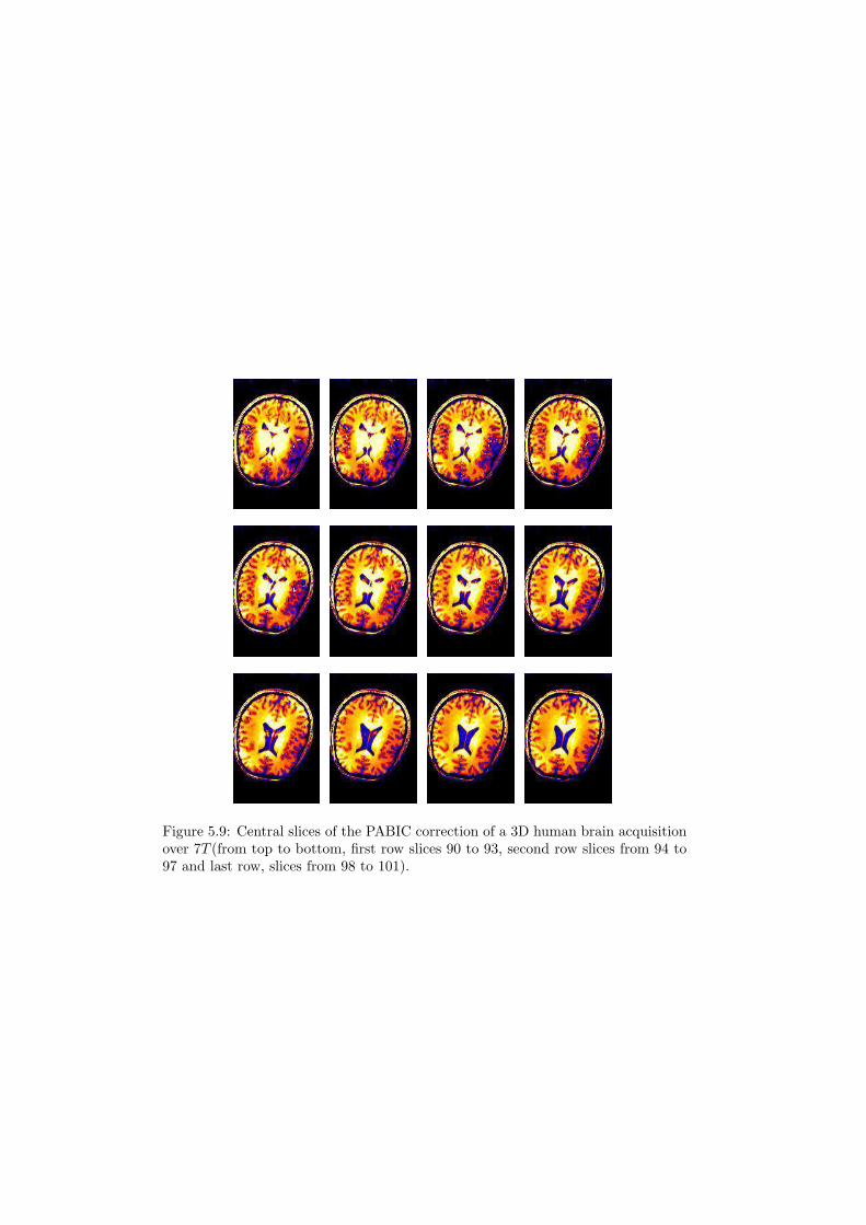
Figure 5.9: Central slices of the PABIC correction of a 3D human brain acquisitionover 7T (from top to bottom, first row slices 90 to 93, second row slices from 94 to97 and last row, slices from 98 to 101).

filtering by a Gaussian filter (specially used in blurring images) or with a Medianfilter, we can achieve good results. In fact, those two filters had been tested andthe results are displayed in this section.

Recall that the Gaussian filter is a wide used filter in signal processing. Gaussiansmoothing is often applied because the noise or the nature of the object observedmight be of a Gaussian probable form. In electronics and signal processing, aGaussian filter is a filter whose filter window is the Gaussian function

x 7→√

a

π· e−a·x2

, (5.5)

or with the standard deviation as parameter

x 7→ 1√2 · π · σ · e

− x2

2·σ2 . (5.6)

Mathematically, a Gaussian filter modifies the input signal by convolution with aGaussian function; this transformation is also known as the Weierstrass transform.Gaussian filters are designed to give no overshoot to a step function input whileminimizing the rise and fall time (which leads to the steepest possible slope). Thisbehavior is closely connected to the fact that the Gaussian filter has the minimumpossible group delay.

Note the Gaussian filter gives more weight to the current pixel position andthen tapers the weights as distance increases according to the Gaussian formula.By weighting a pixels contribution to the final pixel value this filter can better pre-serve edges than the mean filter which specifies equal weights to all pixels withinthe filter window.

Whereas, the median filter is specially useful for removing outliers (that is, ex-treme pixel values). It used ’sliding neighborhoods’ to process an image, that meansit determines the value of each output pixel by examining and m − by − n neigh-borhood around the corresponding input pixel as the median value of them.

The goal of this filtering is to determine quantitatively which was the bestmethod for low-pass filter a 7T acquisition in order to palliate the bias field. Theperformance of the filter solution is simple:

CorrectedImage = AmplitudeFactor × HighContrastAcquisition

F ilteredImage. (5.7)

The test was performed by consecutive filtering the target image changing thevariance and the window size of the filter. The validation is achieved by computingthe Mean Square Error (MSE) between the corrected image and the ground-truth.THis ground-truth had been computed by dividing two different acquisitions ob-tained with different protocols. That is, by dividing one MPRAGE acquisition byone FLASH acquisition. Recalling Chapter 2, Section 2.5, we must clarify that weare actually diving one high-contrast image (MPRAGE) by one obtained with alow-contrast protocol (FLASH)6.

Actually, the main goal of this experiment is to have a 2D map showing theeffects of varying this parameters, and find the best option for bias correction by

6This method had been developed by Xavier Pena Pina at the EPFL, with the collaborationof Siemens Research Group site at the CIBM, Lausanne.

low-pass filtering.

This time, the original image has not only been masked by setting a simplythreshold. Besides, after the threshold that let us avoid the background (as seenbefore), the image was ’skull stripped’ using BET7 algorithm. Skull stripping com-monly refers for Intracranial segmentation, and it segments the brain tissue (cortexand cerebellum) from the skull and non-brain intracranial tissues in magnetic res-onance (MR) images of the brain. So that, it isolate brain from extra-cranial ornon-brain tissues. Skull stripping is an important preprocessing step in neuro-imaging analysis because brain images must typically be skull stripped before otherprocessing algorithms such as registration, tissue classification, or bias field correc-tion can be applied.

Besides, the masked and skull stripped image has also been de-noised. We mustsay that In order to illustrate this part of the process, we take a single slice of the3D volume (see Figure 5.10). So that, the images used for this test are:

(a) (b)

Figure 5.10: 7T MPRAGE acquisition of human brain masked by direct threshold(a) and same acquisition skull stripped and de-noised (b) . (Both in sagittal view).

The skull-stripped and de-noised image, (b), when filtered, is compared to ourground-truth. And this ground truth is, by its axial view (see Figure 5.12).

In resume, the processing chain for this low pass filtering method is shown inFigure 5.11.

Figure 5.11: Block diagram of the LPF method proposed

7BEt algorithm belongs to the FSL Software Library. FSL is a comprehensive library of analysistools for FMRI, MRI and DTI brain imaging data. FSL is written mainly by members of theAnalysis Group, FMRIB, Oxford, UK. It can be found in http://www.fmrib.ox.ac.uk/fsl/fsl

Figure 5.12: Ground truth for correction goodness’ quantitative comparison. Onesingle slice of a 3D volume in its axial view. Ground truth obtained by divingMPRAGE acquisition by parallel FLASH acquisition

Let’s start with the process. In the image we can note even in the inner partof the brain there are some morphological peculiarities than can make impede thecorrect estimation of the bias and, thus, its correction. SO our aim is to removethem before the estimation.

The first step is to mask the image by direct threshold. This masking process, apart for removing the background, can be used to remove high frequency artifactsis the image due to tissue transitions. This tissue transitions are characterized byhaving high gradient value. Thus, one way to localize them is by computing thegradient of the image. With this process we can get some extra information thancan help us in the correction. But, before computing the gradient of the image, alow-pass filter is applied as the artifact we want to erase are at high frequencies.

After that, the BET algorithm is applied (see [12]), so that we remain with theinner part of the brain, without skull. Finally, we apply and de-noising filter. Atthis point, our image is ready for our purpose: the extraction of the bias field bylow-pass filtering.

5.3.1 Results and Validation of the Method

The first filter tried is the Gaussian filter. By changing the variance and the windowsize values, we consecutively filter the corrupted image. For each case, and followingthe hypothesis that the bias field is estimated by the low-pass filtering, we computethe division of the original image by its filtered sample (as shown in 5.3. After that,the Minimum Square Error between the ground truth and the correction calculated.So that, considering the variance values ranging from 1 to 25 and the window sizesmoving from 1 to 80, the following results are obtained:As we can see in the images, the time elapsed in simulation increases while increas-ing the window size of the filter. This is a result we should expect. In fact, thisfilter is applied to an image in a two phase approach. First the horizontal directionis filtered using the above filter in a similar manner to a convolution filter by takingeach pixel in the image, centering the filter on that pixel (the middle value) and thenmultiplying the pixel values by the weight at each filter location followed by a finaldivide to get the resulting new pixel value. This process is then repeated verticallyon the horizontally processed image to create the final image. So, growing windowsize, will grow the length of the convolution and, thus, the time of computation.

(a) (b)

Figure 5.13: Evolution of the MSE between ground truth and image corrected bylow pass filtering method when changing the variance and the window size of thefilter (a) and evolution of the time elapsed in simulations (b). The low pass filterapplied is the Gaussian filter. (variance values from 1 to 25 and window sizes from1 to 80).

However, if we compare this time with the one needed to perform PABIC correctionin the same image, we see the low-pass filtering is a faster method for correction.In fact, the mean time of computation in this case is around 2 minutes, whereaswhen running PABIC correction was around 14 minutes in a 2D image and aroun40 minutes in a 3D one.

One consideration must be done at this point. Window size of the filter is nor-mally related to the variance. Actually, it was not necessary to cover all the sigmavalues from 1 to 25 changing at each time the window size from 1 to 80. It shouldhave been enough to change the variance from value 2 to 20 in steps of 2, and then,for each variance value, change the window size from 3× variance to 5× varinacein steps of the variance value. Nevertheless, the complete coverage has been donein order to plenty test the method.

If we focus now in the MSE graphic, we realize we do not get acceptable valuesfor the Mean Square Error between the corrected image and the image assumed asground-truth. Thus, we can achieve from here, the filtering by Gaussian filter is notenough for estimate the bias at high field acquisitions. However, we can see thatconsidering variance values over 10 gives us a MSE up to 8, whereas if we constraintour filter with variance values around 5 can give us some acceptable results in thequantitative comparison with the ground truth. Thus, when low-pass filtering witha Gaussian filter, we must consider variance σ = 5 and window size between thevalues window = (15, 25).

After this trial, the Median low-pass filtering was tested for bias estimation andcorrection in 7T MR images.

As said in the previous section, the Median filter uses ’sliding neighborhood’ todetermine the output pixel brightness value. Figure 5.14 shows an example of themedian filter application, as in this case, habitually a 3x3 median filter is used. TheFigure 5.14 (a) presents the concept of spatial filtering based on a 3x3 mask, whereI is the input image and O is the output image. In Figure 5.14, the median valueis determined by placing the brightness in ascending order and selecting the centervalue. The obtained median value will be the value for that pixel in the outputimage.

(a)

(b)

Figure 5.14: 3× 3 median filter operation. In (a) some samples of input pixel andits neighboring are displayed. The bright value of the output pixel is computed asshown in (b).

So that, an as the Median filter8 is supposed to be a more robust method thanthe traditional linear filtering, because it preserves the sharp edges, we expect toachieve a better bias estimation than when applying Gaussian filtering.

Nevertheless, the tests with Median filtering did not give better results. Actu-ally, the main problem of the median filter is its high computational cost (for sortingN pixels, the temporal complexity is O(NlogN), even with the most efficient sortingalgorithms). When the median filter must be carried out in real time, the softwareimplementation in general-purpose processors does not usually give good results.

Besides, even having the complexity of the algorithm increased as well as thecomputation time by a factor of O(NlogN), the correction is neither good in termsof intensity homogeneity.

5.3.2 Summary of Bias Correction with Retrospective Meth-ods

Two different retrospective methods for bias correction in 7T MR acquisitions hadbeen tested in this section: the Parametric Bias Correction (PABIC) and the Low

8Median filter is the nonlinear filter more used to remove the impulsive noise. Median filteris a spatial filtering operation, so it uses a 2-D mask that is applied to each pixel in the inputimage. To apply the mask means to center it in a pixel, evaluating the covered pixel brightnessand determining which brightness value is the median value

Pass Filtering approach.

Even if none of the methods plenty achieve the bias correction desired in theimage, one comparison between them can be done.

PABIC method is good to deal with multi-class images, which is one of themain drawbacks when trying to correct the bias directly from a brain MR image.This pretty good behavior is due to its parallel segmentation process (which is notdone with the low pass filtering approach). Besides, PABIC parametrizes the biasfield, giving it in terms of the p− vectors so it can be recursively run, giving themas a initial point for the next step. Otherwise, the computation time became animportant drawback when using this method for bias correction in 3D images. Thetime elapsed in simulations are quite acceptable for 2D acquisition but not for 3Dimages, as it increases nearly exponentially. Nevertheless, it can be reduced byforcing PABIC to start with a certain p-vector value (normally our ground truthvector). However, even in this case, in does not reach good results as it is inca-pable of found a energy global minimum, remaining most of the times in a localminima of the energy function. This is not the case for the Low-Pass filter approach.

The main advantage of the Low Pass Filter for bias correction is that this methodis much faster than PABIC (time elapsed in computation with this approach isnearly then time faster than PABIC). Besides, the simplicity of the algorithm makeshim a good option for image bias correction. However, the correction achieved bythis filtering is worse than the obtained with PABIC. In fact, this method doesnot parallel segment the image so is harder to find the tissue boundaries even if agradient filter is used. Actually, the LPF method is good for correcting single-classimage9. Nevertheless, its strength is weak when a multi-class image are considered.

Despite what we could had imagine before trying the correction by one of thoseretrospective methods, nor PABIC neither the Low Pass Filtering approach, performgood bias correction in 7T acquisitions. It is due to the fact that the assumptionsof smoothness an slow variation are no longer valid. This leads us to say that amethod to correct the bias directly from the acquisition with no other informationis not suitable for acquisitions at high field strength (i.e. over 7T ). Some additionalinformation is needed for achieve an acceptable correction in terms of visual inspec-tion and histogram computing.

Actually, as we can see, there is not only bias in the low-frequency band, buta mixture of undesired bias field and important information. Both are difficult toseparate without no a priori information.

Following this idea, a new method is presented in next Chapter. This methodtake profit from the acquisition of an RF map at the same time of the image. Thisamp gives us information about the distribution of the field and the flip angle insidethe brain, thus, information about the bias field added to the image.

9Recall for further information the master thesis Bias Field Correction in Magnetic Resonancesof a Rat Brain [40]

Chapter 6

A New Prospective SolutionUsing the RF Mapping

The main goal of this Master Thesis is to estimate and eliminate the bias field addedin the MR acquisitions obtained at high fields (over 7T ). In previous sections wehave proved the impossibility of achieve this correction directly from the corruptedimage. The bias field behavior in high field acquisition avoid this fact. Actually, itcannot be seen as an spatially sooth and slow variation. Thus, other information isneeded for this purpose.

Following this aim, we present a new method, based on the acquisition of a RFmap after acquiring the image. Note here we have a compromise. As said in Chapter3.1, the acquisition time is a critical parameter when imaging living tissues. Thepatient must stay longer inside the magnet, at this fact present several drawbacks:

• The patient should avoid moving for acquiring this map in the most accurateway. If he moves, more artifacts will be added to the image. Otherwise, notmoving is not easy, as the magnet is not a comfortable place to lay on.

• Each living tissue presents an maximum absorption rate that cannot be ex-ceed. Actually, when acquiring an MR image, we are applying a magneticfield over the tissues (recall Chapter 2) so we must be careful on not exposethe tissues more time that they can stand.

Actually, with this additional acquisition we are trying to get enough informa-tion to proceed successfully to the bias correction. And, for 7T acquisitions, wherethe bias pattern is not already defined, this is the best possibility for this purpose.

B1 mapping is crucial for the understanding of B1 inhomogeneity patterns andfor quantitative studies such as T1 ad T2 measurements. Because there are differentsources of variation of the field behavior inside the brain, B1 mapping add confi-dence and give important insights into the interpretation of the magnitude images.

It is clear, at this moment, that even susceptibility artifacts appears in the ac-quired images, in there we can also see substantial signal variability due to the B1

inhomogeneity. Actually, as Trong-Kha et al. assess, regions of low signal corre-sponds, directly, to regions with low flip angle and/or low receive sensitivity. Theflip angle variability affects not only the SNR but also the image contrast [34].

Considering different types of acquisition, the effect of the bias field changes.It has been demonstrate that the image contrast will be more severely affected by

53

flip angle variation on T1 weighted images. And, B1 inhomogeneity and the resul-tant spatial variability of the flip angle become progressively more problematic inmulti-pulse sequences (as the MPRAGE). For small flip angle images, the intensitydistributions are approximately symmetric about the centerline of the coil. Withincreasing flip angle, the symmetry in the signal intensity pattern disappears, be-havior caused (as the reader can imagine) by the asymmetry in transmission andreception in the data acquisition process.

So that, to quantify this B1 inhomogeneity, we can compute a map of the flipangle and a map of the receive sensitivity. Different methods had been proposed inliterature for this achievement. In [18] three methods are enumerate:

1. Increment transmitted reference amplitudes and fit as assumed signal behav-ior.

2. Acquire several echoes and calculate the RF distribution by their proper com-bination.

3. Use preparation pulses or additional pulses in various sequences.

All of this methods are implemented in 2D due to time constraints, but in [2] we cansee a method based in two simultaneous acquisitions which is the one used for ourpurpose. Is not extremely difficult to compute those two maps (the flip angle mapand the receive sensitivity one). Following Siemens’ protocol for flip angle mapcomputation, two series of low-resolution images are computed with TR >> T1

and flip angles α0 and 2α0. The acquisitions are one Spin-Echo sequence and oneStimulated-Echo. In this case, the signal intensity at the pixel (x, y) can be writtenas:

Sα(x, y) = ρ(x, y)r(x, y) sin[α(x, y)], (6.1)

andS2α(x, y) = ρ(x, y)r(x, y) sin[2α(x, y)] (6.2)

respectively, where ρ is the proton density, r the received sensitivity and α the localflip angle. A flip angle map can be computed from the signal intensity ratio ofthe two series as follows [34]:

α(x, y) =S2α(x, y)

2 · Sα(x, y). (6.3)

Then, a map of the product of the proton density and the receive sensitivity can becomputed from the flip angle map using 6.1:

ρ(x, y)r(x, y) =Sα(x, y)

sin[α(x, y)]. (6.4)

Finally, a measure of the receive sensitivity can be generated from this map bylow-pass filtering (with a 2D boxcar filter) and normalizing between 0 per cent and100 per cent.

In principle, two measurements with different nominal flip angle are sufficientfor determine the flip angle value α. However, since the resulting flip angle is de-termined from the linear regression of results of all measurements, the acquisitionof the RF maps with more nominal angles reduces the sensibility of the calculate αvalues of the noise [18]. So, we must prevent that this method for calculate the flipangle and sensitivity map from two different sets of images with nominal flip angles

α0 and 2α0 is theoretically accurate for local flip angle α ranging between 0◦ and180◦. If the local flip angle exceeds 180◦, this method can no longer determine thecorrect flip angle. Actually, signal intensity not only decreases in regions with smallflip angles but also in regions with angles larger than 90◦/180◦, where the spins areover-flipped.

At this point, it is almost clear that to correct effects of the RF inhomogeneitiesin 3D data sets it is necessary to have knowledge of the field distribution inside thesample. Thanks to the Siemens’ acquisition protocol we can obtain two differentmaps from this B1 distribution, the (1) magnitude B1 map and (2) the flip anglemap, which is the relative spatial phase pattern for received and transmitted field.

6.1 Magnitude B1 Mapping and Flip Angle Map-ping

In Chapter 3.1, we have presented the way of modeling the signal intensity in eachvoxel of the image. Assuming that for each voxel we can explain signal intensitymodulation as:

I ∝ ρ sin(V |B+1 |γτ)|B−

1 |, (6.5)

where we can see the influence of the transmitted filed ( |B+1 |) and the received one

(|B−1 |).

The way to determine the |B1| and calculate its map is by fitting the modulationof the signal intensity with a sinusoidal function. Once this map is calculated isstraightforward to determine the actual flip angle at each pixel location of an GEacquisition [37]. Actually, in [37] an experimentally examination of the 7T RF coilinterferences between different coil elements is performed, giving special importancein phase spatial distribution. In Appendix C the main formulas are transcribed forinterested readers.

An example of this two maps can be seen in Figure 6.1, where Figure 6.1 (a)in the B1 magnitude map and the Figure 6.1 (b) shown the flip angle map. Inthis approach, only the flip angle map had been used as it the less corrupted byinhomogeneities.

In this images, we can suppose (as Jinghua prove in [17]), that any inhomo-geneity in the flip angle map is due only to the B1 inhomogeneity. In fact, B0

inhomogeneities can impact the signal intensity, but do not directly influence theflip angles obtained. In this assessment lean this new approach to bias correction.We know the flip angle map is only corrupted by the B1 inhomogeneity so, eachinhomogeneity in this map will be due to this artifact. Thus, this flip angle map is,simply, a map of the inhomogeneity we get when imaging a living tissue.

(a)

(b)

Figure 6.1: Single slice representation of the computed B1 magnitude map (a) andcomputed flip angle map (b) from an human brain at 7T .

6.2 Bias Correction using the RF Mapping

As seen before, for correcting an high-field MRI acquisition we need some additionalinformation. Until now, and for low-field acquisition, the correction was performeddirectly from the corrupted data by estimating the bias due its smoothness andslow variation. Nevertheless, this direct correction cannot be achieved in high-fieldacquisition. Some additional data is needed. And, following this aim, we present amethod based on the double acquisition of an image and the RF map (also knowas flip angle map).

The test were performed over one MPRAGE 3D acquisition supplied by theSiemens Research Center in the CIBM. A B1 magnitude map and a flip angle mapwere also supplied. The transverse (axial) MPRAGE acquisition is composed by160 slices of 216×256 pixels each. This image is presented in Analyze 7.5 format asit is an high dynamic range image (HDR). In the Analyze coordinate system, withthis acquisition we get:

1. 160 transverse slices laying on the xy plane, each of 216× 256 pixels.

2. 216 sagittal slices laying on the zy plane, each of 256× 160 pixels.

3. 256 coronal slices on the zx plane, each of 216× 160 pixels.

The test wee performed over a Intel(R) Core(TM)Duo CPU 6600 @2.40GHz, 1.98GBof RAM, but in this case, the time elapsed in simulation was not computed. Thistime is much higher than the one needed for retrospective corrections, but, in con-trary, the correction performed in piecewise better. One consideration must bedone: these tests were performed over a 3D acquisition of high dynamic range sothat, the amount of data is much bigger than the one used for validate other cor-rection methods. Thus, having increased the time of computation is specially dueto this fact.

The algorithm for the correction is based in nearly the same concept used forcorrecting image with low-pass filtering. The corrupted image, after been masked,skull-stripped and de-noised is divided by the flip angle map and finally multipliedby the received field contribution. This last multiplication is performed becausewhen dividing the corrupted image by the flip angle map, we loose some contrast.A block diagram can be seen in Figure 6.2:

6.3 Results and Validation of the Method

Following the algorithm of bias correction, the MPRAGE acquisition was maskedby setting a threshold. After that, the skull stripping was performed using (as inthe case of the Low Pass Filter approach) the BET algorithm from the FSL Library.We must say that this method for skull stripping is not the only one. Actually inthe literature, we can find several methods for brain extraction that seem to workeven better that BET algorithm. The choice of this one was done because BETalgorithm is a method fully-automatized and fast and easy to use. Even thought,we might have test some others. However, due to time constraints, only this onewas tested. It means that some other protocol can be used that might improvethe result or the time of computation. This can be seen as a future work for theimprove of the algorithm.

Figure 6.2: Block diagram of the method proposed. Bias Correction by RF mapping

Once the image is masked and skull-stripped, it is de-noised to facilitate thecorrection. Actually, by de-noising we erase some unwanted effects that might beconfused as bias. We must say that the flip angle map was also masked for remov-ing all the background. Besides, we cannot forget the importance of having theimages well registered. Actually, we are dividing pixel-by-pixel one image by itscorresponding flip angle. If the images are not accurately registered, we might wedividing one pixel by flip angle value of the neighboring pixel and the results willbe distorted.

The correction was performed over a 3D volume. Nevertheless, to illustrate thissection, only several slices of the volume are presented. In figure 6.3, the three views(axial, sagittal and coronal view) of a single slice of the volume used for the testare represented:

The result of the algorithm is seen in Figure 6.4:

The validation of this method had been performed only by visual inspection.As we can see in the image 6.4, even the bias correction is not totally performed,the image had been corrected in intensity inhomogeneities. We are still missingsome good results in the hypothalamus and the temporal lobe. This can be dueto the fact that the acquisition of the flip angle map was not plenty co-registeredwith the MPRAGE acquisition. In fact, for achieve this registration, the flip anglemap was switched by a 10 degree angle. And when we are talking about one ’anglerepresentation’ image, this fact is not negligible.

This fact can also explain the lost of contrast of the image. Even after multi-plying the image by the contrast correction factor which is the contribution of thereceived field to the image (i.e. B−

1 ), the contrast is not well recovered. Never-theless, the improvement of this method in comparison with the retrospective ones

Figure 6.3: Axial (transverse), sagittal and coronal view of a single slice of a 3Dvolume MPRAGE acquisition of 216x256x160 pixels before the correction using theRF mapping.

Figure 6.4: Axial (transverse), sagittal and coronal view of a single slice of a 3Dvolume MPRAGE acquisition of 216x256x160 pixels after the correction using theRF mapping.

analyzed in this report, is that the brightness of the image seems to be more homo-geneous than in the other cases. We have been able to erase the bright spot in themiddle of the image, attenuating its value and, besides, we have achieved a betterhomogeneity in almost all the image (even though we have lost contrast).

This is not a perfect result, but, however, it is a encouraging one. In fact, afterhaving tried several methods for achieve this bias corrections which was the maingoal if this Master Thesis we realized that none of the actual ones work, so, a needmethod is needed. Bias Correction by using the RF mapping can be this neededone. As a future work, one improvement of this method can be tried, in orderto completely parametrize the bias inside the brain, so that will allow the totalcorrection of the bias without contrast lost.

6.4 Summary of A New Prospective Solution Us-ing the RF Mapping

In this Chapter a new prospective solution has been presented. This new approachlean on the needing of having some additional information for properly achieve thebias correction in 7T MRI acquisitions.

Actually, for low-field acquisitions, we are able to correct the bias directly fromthe corrupted data, as this bias has smooth and slow varying behavior so that inlays on the low-frequencies of the image. Due to this fact, Low-Pass filtering canbe a good and fast approach for this purpose.

In high-field acquisition, the assumption made for the bias is no longer valid,so some additional information is needed for perform the correction. The approachpresented in this section, take profit of the acquisition (at the same time of theimage) of a RF map (or flip angle map). This map is a related to the angle ofprecession of the spin in the living tissue and, therefore, any inhomogeneity in thismap will be showing the inhomogeneity due to the bias field.

Some tests had been performed and even the result are not completely per-fect, they give a new line of investigation for future work on bias correction in 7Tacquisitions.

Chapter 7

Conclusions and FutureWork

The aim of this project was to remove the bias distortion, so called bias field orintensity inhomogeneity, from MRI images of human brain acquired with 7T MRmachines. The ultimate goal was, obviously, to supply the medical community witha tool which could allow them to diagnose, in a reliable way, possible human braindiseases as well as help them understand its behavior by having the chance of givingand accurately insight into the physiological condition of the brain.

The first attempt in this way was to test reliable methods in bias correction un-der 3T that were plenty proved in this achievement. The PABIC and the Low-PassFilter were tested. Both rely in the assumption of smoothness and slow variationof the bias field along the images. Even its capacity of extrapolate the bias all overthe image (i.e. the region corrected can be bigger than the region measured toestimate the bias), none of them can completely ensure the success in bias estima-tion and bias correction. Actually, as the bias does not have smoothness behavioranymore it cannot be approximate by Legendre Polynomials or other smooth basisfunctions. So that, PABIC present several problems to reach the global minimumof energy needed when estimating the bias. Besides, the bias field presents a multi-plicative effect over the image intensity that cannot be transformed in additive bylog-transformation. This avoid us getting good results by low pass filtering the im-age by Gaussian or Median filters, which was a point we want to prove following thework done at the EFPL by Xavier Pena Pina over 9.4T acquisitions in rat brains [40].

This fact can be seen as the main contribution of this master thesis. We havedemonstrate that the methods for performing bias field correction in acquisitionswith field less than 3T are no longer useful for correcting 7T acquisitions. All theconclusions and results are based in the fact that at 7T the bias can not be assumedas a slow and smooth variation all over the image.

Actually, the main drawback is that, when increasing field strength (speciallyif we work with high field acquisitions (> 7T )), the bias field starts having awave behavior that makes impossible its approximation by an smooth function asit is strongly dependent in the dielectric effects, and the conductivity of each tissuein the brain. Artifacts due to B0 and B1 inhomogeneity are severe in ultra-highmagnetic field MRI and experimental and/or numerical mapping of the B0 and B1

inhomogeneity is important in identifying their origin. Detailed characterization ofthese effects is an important step in the development and assessment of B0 and B1

61

inhomogeneity correction methods. In this fact lean the new prospective approachpresented in this Master Thesis.

The idea of this method is to acquire extra information during the imaging pro-cess, so that it can help in the bias correction. The main advantage of it (whencomparing with other approaches) is that this correction, if well used, could be moreconsistent than the other ones. Actually, it relies in an analytical approach of theintensity inhomogeneity at high fields strengths. In fact, we have seen during thisreport that correcting the bias field directly from the corrupted data has seriouslimitations (specially at high-fields).

Nevertheless, this feature has some drawbacks. Its is computationally compli-cated (specially if we compare it with the Low-Pass Filter approach) as we aredealing with a big amount of data. And, at this point of the research, we have notbeen able to assure neither in this case a perfect bias correction in 7T acquisitions.However, despite this fact, the results are enough encouraging to keep working inthis line.

In this report we actually present a draft for a method which can combine thetwo lines of investigation in bias correction we found nowadays: the prospective andthe retrospective methods. And, as a future work, some new improvements can bedone as a future work.

• A accurate parametrization of the bias should be deeply studied so the B1

mapping can be fully defined. We cannot forget (as said in Chapter 5.1) thatthe image registration becomes crucial at this point. When comparing theimage with its RF map, we need all the pixel/voxel to have perfect correspon-dence in both images.

• Improve the steps prior to the image division. That is, improve the skullstripping and the de-noising, as well as the masking. In fact, the less artifactwe get in the image (even if they are not due to the bias) the better resultswe can get. Several methods are proposed in the literature in this sense, evenwe had only tried the BET algorithm due to time constraints.

• To combine previous estimation and post-correction force us to get speciallyknowledge of the nature of the images (both MPRAGE acquisition and RFmap). An effort combination between physics and signal processing researchgroups had permitted us to outline this new approach. However, keep thisline of research could lead us to successfully estimate an remove the bias inthis high field acquisitions.

As the last point of this Chapter, note that, even if this report focus in MRIacquisition of human brains images, the bias appears in all MR imaging techniques,whereas we are imaging the brain or other parts of the body. So that, the con-clusion assessed for the specific case of the brain, can be extrapolate to other MRacquisitions. So that, erasing the bias in high field acquisition could give us, notonly a good insight of the brain but the whole human body.

Appendix A

Radio-frequency PowerRequirements of HumanMRI

The values obtained in this Appendix rely on the study carry out by L.Tang inhis paper [32]. The values had been obtained by a simulation model, a 16-elementTEM resonator based on multi-conductor transmission line theory loaded by ananatomically detailed head mesh.

A.1 Power an SAR Calculations

The input power from the RF coil can be written (deriving it from MAxwell equa-tions) as:

Pinput = Pabs + Prad +σ

2

∫ ∫ ∫

v

|−→E |2dv +12

∫ ∫

s

(−→E ×−→H ∗)ds, (A.1)

with Pabs and Prad the absorbed and radiated power, σ is the conductivity and−→E

and−→H are the electric and magnetic fields respectively.

The RF power absorbed is related with the flip angle (as we have seen is linearlyproportional to the circularly polarized component B+

1 we can only consider theabsorbed power. So changing the continuous integration by summation we obtain:

Power =∑

i

∑

j

∑

k

[12σ(i,j,k) × (E2

x(i,j,k) + E2y(i,j,k) + E2

z(i,j,k))], (A.2)

where σ(i,j,k) in [S/m] is the conductivity at the (i, j, k) location. Ex, Ey and Ez

are magnitudes of the electric field components in the x, y and z directions andexpressed in [V/m].

The SAR is modeled as:

SAR(i,j,k) =12

σi,j,k(E2x(i,j,k) + E2

y(i,j,k) + E2z(i,j,k))

ρ(i,j,k), (A.3)

where ρ(i,j,k) is the tissue density at location (i, j, k). SAR has the unit [W/Kg].

63

Appendix B

1D Electromagnetic (EM)Theory for Wave Interference

At this point, it is proved that the highest B1 inhomogeneity that occurs in a samplewhen acquiring an MRI at high field is due to the wave behavior of the field insidethe brain. Actually, as the sample dimensions represent a larger percentage of awavelength (λ), intermediate and far field effects, including wave propagation, be-come more important. At it is this presence which requires the use of the full-wavesolution of Maxwell equations. In this Appendix, 1D theory is explored to explainthe patterns of the interference sources in a phantom. It has been performed in [7].

Whereas the coil used are volume coils, arrays surface coils or single surface coil,the wave interference effect, appears when a sample is added in a MRI machine.And this interference, can be constructive o destructive.

The explanation is simple. When a sample is added, and due to the multipleair/tissue we find in the brain, the applied field will suffer numerous reflections,giving a multiple path pattern propagation. One example can be seen in figure B.1:

Figure B.1: Multiple propagation path in rectangular sample with large reflectioncoefficients at boundaries.

In this figure there are represented some of the possible paths where the wavewould propagate. When getting at the boundary a reflection take place. If at thismoment there is no phase difference between the incident wave and the reflected one,

64

we will get a constructive interference and the values of amplitude will be added.By contrary, if there is a 180 phase difference, the interference will be destructiveand the two wave swill cancel them out. Those 2 cases are the extreme ones butwe can find all the intermediate ones that will cause different level of interference.

So, how we can determine the effects of sample properties and size in this propa-gation? Let us consider a plane wave traveling with normal incidence (that is to sayperpendicular) to the sample considering B0 on the z direction, a linearly polarizedB1 in the y direction and a wave traveling on the x direction. The sample is formedby four layers (and it can be extendable) with different physical and electrical prop-erties (see fig. B.2).

Figure B.2: Sample with four different layers and their physical and electrical prop-erties.

Assuming the incident wave in a single direction B(x0) = B(x)y (for facilitatethe computation)we get a general form of the solution for the magnetic field B =B(x)y = By0h(x)y. h(x) is found for solving the wave equation at each layer:

hi(x) = Ci cos ki + Si sin ki, (B.1)

with i = 1, 2, 3, 4 and k the complex wave number defined by:

ki = αi + jβi. (B.2)

In equation B, αi represents the attenuation constant and β−i is the phase constantin the layer. The skin depth δ is related to α as δ = 1/α.

The coefficients Ci and Si are found using the eight boundary conditions [33] atthe interface between layers:

• Initial value at x0.

• Continuity of E and B fields at x1, x2 and x3.

• Perfect conductor condition at x4.

The layer 1 which is the space between the source of the wave and the sample) isassigned free space properties. The layer 2 represents the sample and its conduc-tivity and thickness are varied. Layer 3 assigned for the properties of the free spaceand layer 4 is an absorbing boundary condition.

The experimental results obtained for different test performed to demonstratethe wave behavior of the field inside the sample can be found at [7].

Appendix C

Relative Spatial PhasePatterns for Received andTransmitted B1 Field

In this experiment [37], the study of the RF penetration in human body is performedwith an eight-channel transceiver coil array that allows the use of an identical coilstructure as a volume transmitted coil, multichannel receive coil or multiple singletransmit surface coils. The tests are performed over a phantom.

Without studying to much in depth, for the receive B1 field, the complex imageobtained after 2D Fourier Transform the phase of the raw data from one channelat image coordinate r can be written as:

Φrawi,j = ϕr,B∗1,jrel + ϕ0,j + ϕr,B1com + ϕr,∆B0 + ϕr,res, (C.1)

For the ϕr,B1com term we get:

ϕr,B1com = ϕr,B+1

+ ϕr,B−∗1 com. (C.2)

where j is the channel (or coil element). We can group the terms depending onwhereas they depend or not with the coil topology and situation.

• Coil-specific terms.

– ϕr,B∗1,jrel Is the coil-specific relative spatial phase. This term varies withcoil and spatial position and is the one we want to estimate.

– ϕ0,j Stands for the coil specific zero-order phase and it corresponds toa global phase shift for each channel. It depends on the relative polarposition of the element in the circle formed by the eight coil elements, aswell as on other hardware components inducing phase shifts. It can beeestimate from the average phase of small ROI1 at the center of the samplebecause coils are expected to have the same phase in that location.

• Coil-independent terms. Those terms accounts for B0 inhomogeneities:

– ϕr,B1com is the coil common B1 phase.– ϕr,∆B0 is the ∆B0 phase derived from the phase of the complex ratio

between two images acquired at 10ms and 6ms echo time (TE).1ROI stands for Region of Interest

66

– ϕr,res accounts here for a slight offset of k-space center.

Some of those terms had been estimated. Thus, the coil specific zero-order termsis:

ϕ0,j=arg[ROI∑ praw

j exp(−jγTE∆B0) exp(−j)ϕr,res

|prawj | ], (C.3)

where |prawj | is the pixel-wise form each channel value and arg(|praw

j |) its phase.Finally, the common phase term is estimate under the hypothesis that given thespherical symmetry of the phantom and the eightfold cylindrical symmetry of thecoil structure

ϕr,com = arg(N∑

j

pj,r

|pj,r|), (C.4)

being N the number of coils. The pixelwise raw complex values are defined as:

pj = prawj exp(−jϕ0,j) exp(−jγTE∆B0) exp(−jϕr,res). (C.5)

In the case of the transmitted B1 field we get a similar equation as for theone determined for the receive field but with some additional terms. The phasein complex data collected with coil element j when transmitting RF through coilelement k is:

Φrawi,j,k = ϕr,B−∗1,j rel + ϕr,B+

1,krel + ϕ0,j,k + ϕr,B1com + ϕr,∆B0 + ϕr,res. (C.6)

andϕr,B1com = ϕ+

r,B1com + ϕ−∗r,B1com. (C.7)

Removing the terms ϕ0,j,k , ϕr,∆B0 and ϕr,res from the raw data, we get and easierexpression, which is the apparent phase expression:

Φappi,j,k = ϕr,B−∗1,j rel + ϕr,B+

1,krel + ϕr,B1com. (C.8)

The estimation of the phase expression ϕr,B+1,krel+ϕr,B1com is obtained following:

ϕr,B+1,krel + ϕr,B1com = ϕr,com = arg(

N∑

j

pj,r,k

|pj,r,k| ). (C.9)

Those eight sums are put together in order to estimate ϕr,B1com as:

ϕr,B1com = arg(N∑

k=1

N∑

j=1

pj,r,k

|pj,r,k| ). (C.10)

Finally,each relative coil transmit phase ϕr,B+1,krel is derived from the previous equa-

tions getting:

ϕr,B+1,krel = arg((

N∑

j

pj,r,k

|pj,r,k| ) · (N∑

k=1

N∑

j=1

pj,r,k

|pj,r,k| )∗). (C.11)

Appendix D

Legendre Polynomials

Legendre functions are solutions to Legendre’s differential equation:

d

dx

[(1− x2)

d

dxPn(x)

]+ n(n + 1)Pn(x) = 0. (D.1)

These solutions for n = 0, 1, 2,... (with the normalization Pn(1)=1) form a poly-nomial sequence of orthogonal polynomials called the Legendre polynomials. EachLegendre polynomial Pn(x) is an nth-degree polynomial. It may be expressed usingRodrigues’ formula:

Pn(x) =1

2nn!dn

dxn

[(x2 − 1)n

]. (D.2)

Legendre Polynomials are used to estimate the bias in PABIC (see. Section 5.1) asthey are smooth. This fact in needed because, as Styner assess in [?], the choiceof an orthogonal basis result a better posed condition for changing the parameterspi. Actually, the Legendre Polynomials are just one choice in between the otherpossibilities.An important property of the Legendre polynomials is that they are orthogonalwith respect to the L2 inner product on the interval −1 < x < 1

∫ 1

−1

Pm(x)Pn(x) dx =2

2n + 1δmn, (D.3)

(where δmn denotes the Kronecker delta, equal to 1 if m = n and to 0 otherwise).In fact, an alternative derivation of the Legendre polynomials is by carrying outthe Gram-Schmidt process on the polynomials 1, x, x2, ... with respect to this innerproduct. The reason for this orthogonality property is that the Legendre differentialequation can be viewed as a SturmLiouville problem

d

dx

[(1− x2)

d

dxP (x)

]= −λP (x), (D.4)

where the eigenvalue λ corresponds to n(n + 1). Polynomial at each coordinate aremultiplied to define basis functions as:

Pl(x) =n−1∏

j=0

Plj (xj). (D.5)

68

Appendix E

Optimization with (1+1)-ESalgorithm

styner at al., in [31] had developed and nonlinear estimation for bias parametriza-tion. This algorithm, randomly iterates select a new position in the parameterspace being controlled by a probability function centered at the current position.The algorithm is summarized in [31] as:

rt ∼ N(0, I). (E.1)

xt+1 = xt + atxt, (E.2)

whereat+1 = at · cgrow, if f(xt+1) < f(xopt) (E.3)

at+1 = at · cshirnk, otherwise (E.4)

andxopt = xt+1, if f(xt+1) < f(xopt) (E.5)

xopt = xopt, otherwise. (E.6)

The paremeters cgrow, cshrink, a0 and x0 are given as a input and rt ∼ N(0, I) is amultidimensional random vector of an isotropic normal distribution with zero meanand variance one.

69

List of Figures

1.1 Siemens MAGNET for 7 Tesla acquisitions . . . . . . . . . . . . . . 3

2.1 Longitudinal magnetization and transverse magnetization values fora T1-weighted (a), and T2-weighted (b) images . . . . . . . . . . . . 7

2.2 Types of MRI acquisition . . . . . . . . . . . . . . . . . . . . . . . . 112.3 Transverse, sagittal and coronal view of a FLASH acquisition at 7T

of a human brain . . . . . . . . . . . . . . . . . . . . . . . . . . . . . 132.4 Transverse, sagittal and coronal view of a MPRAGE acquisition of a

human brain . . . . . . . . . . . . . . . . . . . . . . . . . . . . . . . 14

3.1 MPRAGE acquisition of a human brain corrupted by bias . . . . . . 183.2 Histogram of brain tissue with IIH. Figure (a) shows two differ-

ent histograms obtained from BrainWeb-simulated database page(www.bic.mni.mcgill.ca/brainweb) one with noise and without IIH(solid line) and the other with noise and IIH (dashed line). Figure(b) is the histogram from a real brain image. . . . . . . . . . . . . . 22

3.3 Hyper-intense region in the center of the head at 7T and its 3D view . 273.4 Grayscale plots of the transmission field and its circularly polarized

components (a), and the contour plot of βt (b) of the quadraturesurface coil in free space (σ = 0, εr = 1). This plot is a ratio of thetransmission field defined as βt ≡ |B+

t ||B+

t |+|B−t |Image obtained from

paper [16] . . . . . . . . . . . . . . . . . . . . . . . . . . . . . . . . . 28

5.1 2D human brain image used for first test in bias correction withPABIC. Single slice for a 7T MPRAGE acquisition corrupted bynoise and bias (a) and plot of the computed histogram of its axialview (b). . . . . . . . . . . . . . . . . . . . . . . . . . . . . . . . . . . 40

5.2 2D human brain image used for first test in bias correction withPABIC. Single slice for a 7T MPRAGE acquisition corrupted bynoise and bias (a) and the mask used for avoiding background (b). . 41

5.3 Evolution of the elapsed time in simulation while changing pre-filtervariance . . . . . . . . . . . . . . . . . . . . . . . . . . . . . . . . . . 41

5.4 2D human brain image corrected with PABIC (a) and its grayscaleprofiles. Horizontal profile (b) and vertical profile (c). . . . . . . . . 42

5.5 Evolution of the p-vectors while increasing the number of maximumiterations allowed. . . . . . . . . . . . . . . . . . . . . . . . . . . . . 42

5.6 2D human brain image corrected with PABIC (a) and the evolutionof the p-vectors while increasing the number of iterations up to 40000(b). . . . . . . . . . . . . . . . . . . . . . . . . . . . . . . . . . . . . . 43

5.7 Slice of a 3D volume human brain image corrected with PABIC (a)and its intensity histogram (b). . . . . . . . . . . . . . . . . . . . . . 44

70

5.8 Vertical (a) and horizontal (b) profiles of gray values of one slice of a3D human brain acquisition at 7T after PABIC correction with thirddegree of Legendre polynomials. . . . . . . . . . . . . . . . . . . . . . 45

5.9 Central slices of the PABIC correction of a 3D human brain acqui-sition over 7T (from top to bottom, first row slices 90 to 93, secondrow slices from 94 to 97 and last row, slices from 98 to 101). . . . . . 46

5.10 7T MPRAGE acquisition of human brain masked by direct threshold(a) and same acquisition skull stripped and de-noised (b) . (Both insagittal view). . . . . . . . . . . . . . . . . . . . . . . . . . . . . . . . 48

5.11 Block diagram of the LPF method proposed . . . . . . . . . . . . . . 485.12 Ground truth for correction goodness’ quantitative comparison. One

single slice of a 3D volume in its axial view. Ground truth obtainedby diving MPRAGE acquisition by parallel FLASH acquisition . . . 49

5.13 Evolution of the MSE between ground truth and image correctedby low pass filtering method when changing the variance and thewindow size of the filter (a) and evolution of the time elapsed insimulations (b). The low pass filter applied is the Gaussian filter.(variance values from 1 to 25 and window sizes from 1 to 80). . . . . 50

5.14 3× 3 median filter operation. In (a) some samples of input pixel andits neighboring are displayed. The bright value of the output pixel iscomputed as shown in (b). . . . . . . . . . . . . . . . . . . . . . . . . 51

6.1 Single slice representation of the computed B1 magnitude map (a)and computed flip angle map (b) from an human brain at 7T . . . . 56

6.2 Block diagram of the method proposed. Bias Correction by RF map-ping . . . . . . . . . . . . . . . . . . . . . . . . . . . . . . . . . . . . 58

6.3 Axial (transverse), sagittal and coronal view of a single slice of a3D volume MPRAGE acquisition of 216x256x160 pixels before thecorrection using the RF mapping. . . . . . . . . . . . . . . . . . . . . 59

6.4 Axial (transverse), sagittal and coronal view of a single slice of a3D volume MPRAGE acquisition of 216x256x160 pixels after thecorrection using the RF mapping. . . . . . . . . . . . . . . . . . . . . 59

B.1 Multiple propagation path in rectangular sample with large reflectioncoefficients at boundaries. . . . . . . . . . . . . . . . . . . . . . . . . 64

B.2 Sample with four different layers and their physical and electricalproperties. . . . . . . . . . . . . . . . . . . . . . . . . . . . . . . . . . 65

Bibliography

[1] Abduljalil AM, er al., Enhanced gray and white matter contrast of phasesusceptibility-weighted images in ultra high field magnetic resonance imaging.Journal of Magnetic Resonance Imaging, vol.18, pp:284-290 (2003).

[2] Akoka S. et al., Radiofrequency map of an NMR coil by Imaging. MedicalResonance in Medicine, vol.11, pp:437-441. (1993).

[3] Axel, L., Constantini, et al., Intensity Correction in surface coil MR imaging.Am. J. Roentgenol, vol. 148, pp: 418-420 (1987).

[4] Bach Cuadra, Meritxell Atlas-based segmentation and classification of mag-netic resonance brain images. Thse EPFL, no 2875 (2003). Dir.: Jean-PhilippeThiran.

[5] Belaroussi B, et al,. Intensity non-uniformity correction in MRI: Existing meth-ods and their validation. Medical Image Analysis, vol.10, pp: 234-246 (2006).

[6] Ayres, Fan. A Variational Approach to MRI BIas Correction.

[7] Caserta Jim, et al. Reduction of wave phenomena in hihg field MRI experimentsusing absorbing layers. Journal of Magentic Resonance, vol. 169, pp.187-195(2004).

[8] Clare S., et al., Compensating of B1 inhomogeneity using active transmit powermodulation. Magnetic Resonance Imaging, vol.19, pp:1349-1352 (2001).

[9] Christoforidis GA, et al., High resolution MRI of the deep brain vascularanatomy at 8 Tesla: susceptibility-based enhancement of venous structures. J.Compt. Assist. Tomogr. vol 23, pp:857-66 (1999).

[10] R.Deichmann et al., Optimization o 3D MP-RAGE sequeces for structuralbrain imaging. NeuroImage. Vol.12, pp:112-127(2000).

[11] R.Deichmann et al., RF inhomogeneity compensation in structural brain imag-ing Magnetic Resonance in Medicine, vol.47: pp.398-402 (2002)

[12] FSL Software Library Analysis Group, FMRIB, Oxford, UK.http://www.fmrib.ox.ac.uk/fsl/fsl

[13] Hashemi Ray, et al., The Basics 2ED, 2004.

[14] Hiroaki M, et al., Imaging of the dielectric resonance effects in high field mag-netic resonance imaging. Journal of applied physics, vol.97. 10R305 (2005).

[15] National Library of Medicine Insight Segmentation and Registration Toolkit.http://itk.org

72

[16] Jinghua, Wang et al., Polarization of the RF field in human head at high field:a study with quadrature surface coilat 7.0 T Magnetic Resonance in Medicine,vol.48, pp.362-369 (2002).

[17] Jinghua, Wang et el., Factors Influencing Flip Angle Mapping in MRI: RFPulse Shape, Slice-Select Gradients, Off-Resonance Excittaion and B0 Inho-mogeneities. Magnetic Resonance in Medicine, vol.56, pp.463-468 (2006).

[18] Jiru, F. et al., Fast 3D Radiofrequency Field Mapping Using Echo-PlannarImaging. Magnetic Resonance in Medicine, vol.56, pp.1375-1379 (2006).

[19] Lauterbur, et al., Image formation by induced local interactions: examples ofemploying nuclear magnetic resonance. Nature, vol 242, pp:190191 (1973).

[20] Lei H, et al. in vivo P-31 magnetic resonance spectroscopy of the human brainat 7 Tesla: an initial experience. Magnetic Resonance in Medicine, vol.49, pp.199-205 (2003).

[21] Lin, F-H., et al. A wavelet-based approximation of surface coil sensitivity pro-files for correction of image inhomogeneity and parallel imaging recosntruction.Human Brain Mapping, vol.19, pp: 96-11 (2003).

[22] Liney G., et al., A simple method for the correction of endorectal surface coilinhomogeneity in prostate imaging. Journal of Magnetic Resonance Imaging,vol.8 ,pp:994-997 (1998).

[23] McRobbie D., et al., MRI, From picture to proton, 2003

[24] S.Prima et al., maximum likelihood estimation for the bias field in MR im-ages:Investigating different modelings for the imaging process. Proc.Med.ImageComp.Computer-Assist. Intervention - MICCAI 2001: 4th Conf.,Utrech, TheNetherlands, vol.2208, pp.811-819 (2001).

[25] Qing X.yang et al., Analyis of wave behaviour in lossy dielectric samples athigh field. Magnetic resonance in Medicine, vol 47: pp.982-989 (2002). DOI:10.1002/mrm.10137.

[26] S.Rice. Mathematical Analysis of Random Noise. Bell Sys. Tech. J., vol. 23,pp:282-332, July 1944.

[27] Jan Grimm, et al., MR imaging at 7T. Center for Molecular Imaging Re-search.Department of Radiology, Masachussets General Hospital. Medical So-lution, January 2000.

[28] J.Sijbers et al., Maximum-likelihood estimation of Rician distribution parame-ters. IEEE Transactions in Medical Imaging, vol. 17, No. 3,pp.357-361, June,1998.

[29] J.G. Sled et al., A nonparametric method for automatic correction of intensitynonuniformity in MRI data. IEEE Transactions in Medical Imaging, vol.17,No 1, pp.87-97,February 1998.

[30] Stanislav Skora,, K-space formulation of MRI.http://www.ebyte.it/library/educards/mri/K-SpaceMRI.html March, 2005.

[31] Martin Styner, et al., Parametric Estimate of Intensity Inhomogeneities Ap-plied to MRI. March, 2000.

[32] tang, L. et al., On the Radio-frequency Power Requirements of Human MRI.PIERS on Line, vol.3, No.6, (2007)

[33] Thomas B, et al., Approximate Boundary Conditions in Electromagnetics. BjrnEngquist and Gregory A. Kriegsmann, Eds. (1997)

[34] Trong-Kha et al., Effects of static radiofrequency maggnetic field inhomogeneityin Ultra-High magnetic fiel resonance imaging. Magnetic Resonance Imaging,vol. 24,pp:103-112(2006).

[35] Ugurbil, Kamil. Brain Imaging at 3T and Challenes at 7T University of Min-nesota medical School, Dept. of Radiology, Centre of Magnetic Resonance Re-search. Minneapolis, MN, USA.

[36] Uros Vovk, et al., A Review of Methods for Correction of Intensity Inhomo-geneity in MRI. IEEE Transactions in Medical Imaging, Vol 26, No.3. March2007.

[37] Van de Moortele, Pierre Francois et al., B1 destruvtive Interferences and SpatialPhase Patterns at 7T with a Head Transceiver Array Coil. Magnetic Resonancein medicine. Vol 54, pp.1503-1518 (2005).

[38] Vaughan T, et al., How t do Rf at high fields University of Minnesota Centreof Magnetic Resonance Research. Minneapolis, MN, USA. ISMRM, May 6-12,2006.

[39] Vokurka E., et al. A Fast Model Independent Method for Automatic Correc-tion of Intensity Non-uniformityin MRI data. Journal of Magnetic ResonanceImaging, vol.10, pp: 550-562 (1999).

[40] Pena Pina, Xavier. Bias Field Correction in Magnetic Resonance Images ofa Rat Brain. ITS, Swiss Federal Institute of Technology (EPFL). September2007.

[41] Zujun, Hou. A Review on MR Image Intensity Inhomogeneity Correctio. Hin-dawi Publishing Corporation. Interantional Journal of Biomedical Imaging, vol.2006, pp:1-11. ID 49515, DOI:10.1155/IJBI/2006/49515

[42] http://www.tesisenxarxa.net/TESISUB/AVAILABLE/TDX-0311105-110752//1.INTRODUCCION.pdf,2008