Journal Club: mcDESPOT with B0 & B1 Inhomogeneity

Papers

• Deoni et al. Gleaning multicomponent T1 and T2 information from steady-state imaging data. Magn. Reson. Med. (2008) vol. 60 (6) pp. 1372-1387

• Deoni. Correction of main and transmit magnetic field (B0 and B1) inhomogeneity effects in multicomponent-driven equilibrium single-pulse observation of T1 and T2. Magn. Reson. Med. (2010)

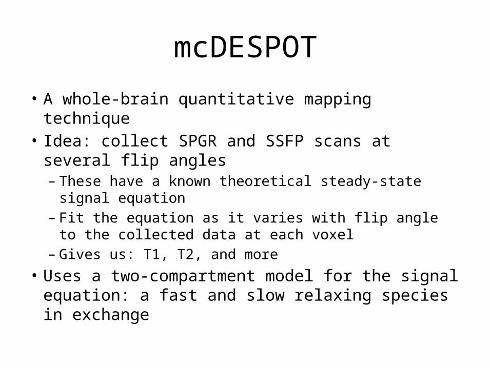
mcDESPOT

• A whole-brain quantitative mapping technique• Idea: collect SPGR and SSFP scans at several flip

angles– These have a known theoretical steady-state signal

equation– Fit the equation as it varies with flip angle to the collected

data at each voxel– Gives us: T1, T2, and more

• Uses a two-compartment model for the signal equation: a fast and slow relaxing species in exchange

scDESPOT Theory

• DESPOT1: SPGR equation– Find M0 and T1, minimize (SSPGR-ŜSPGR)2

• DESPOT2: SSFP equation– Given T1, find M0 and T2, minimize (SSSFP-ŜSSFP)2

€

ˆ S SPGR α( ) =M0 1− E1( )sinα

1− E1 cosα, E1 = e

−TR

T1

€

ˆ S SSFP α( ) =M0 1− E1( )sinα

1− E1E2 − E1 − E2( )cosα, E2 = e

−TR

T2

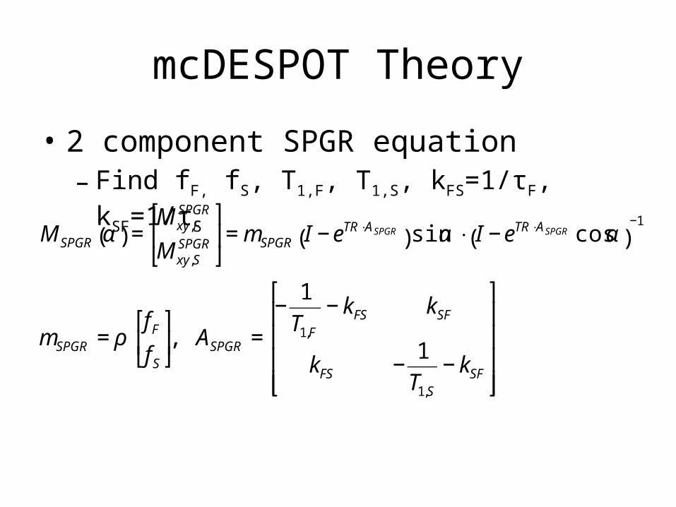
mcDESPOT Theory

• 2 component SPGR equation– Find fF, fS, T1,F, T1,S, kFS=1/τF, kSF=1/τS

€

MSPGR α( ) =Mxy,F

SPGR

Mxy,SSPGR

⎡

⎣ ⎢

⎤

⎦ ⎥= mSPGR I − eTR⋅ASPGR( )sinα ⋅ I − eTR⋅ASPGR cosα( )

−1

mSPGR = ρfF

fS

⎡

⎣ ⎢

⎤

⎦ ⎥, ASPGR =

−1

T1,F

− kFS kSF

kFS −1

T1,S

− kSF

⎡

⎣

⎢ ⎢ ⎢ ⎢

⎤

⎦

⎥ ⎥ ⎥ ⎥

mcDESPOT Theory

• 2 component SSFP equation– Find M0 and T1, minimize (SSPGR-ŜSPGR)2

€

MSSFP α( ) =

Mx,FSSFP

Mx,SSSFP

My,FSSFP

My,SSSFP

Mz,FSSFP

Mz,SSSFP

⎡

⎣

⎢ ⎢ ⎢ ⎢ ⎢ ⎢ ⎢

⎤

⎦

⎥ ⎥ ⎥ ⎥ ⎥ ⎥ ⎥

= eTR⋅ASSFP − I( )ASSFP−1 C ⋅ I − eTR⋅ASSFP R α( )( )

−1

C = ρ 0 0 0 0fF

T1,F

fS

T1,S

⎡

⎣ ⎢

⎤

⎦ ⎥

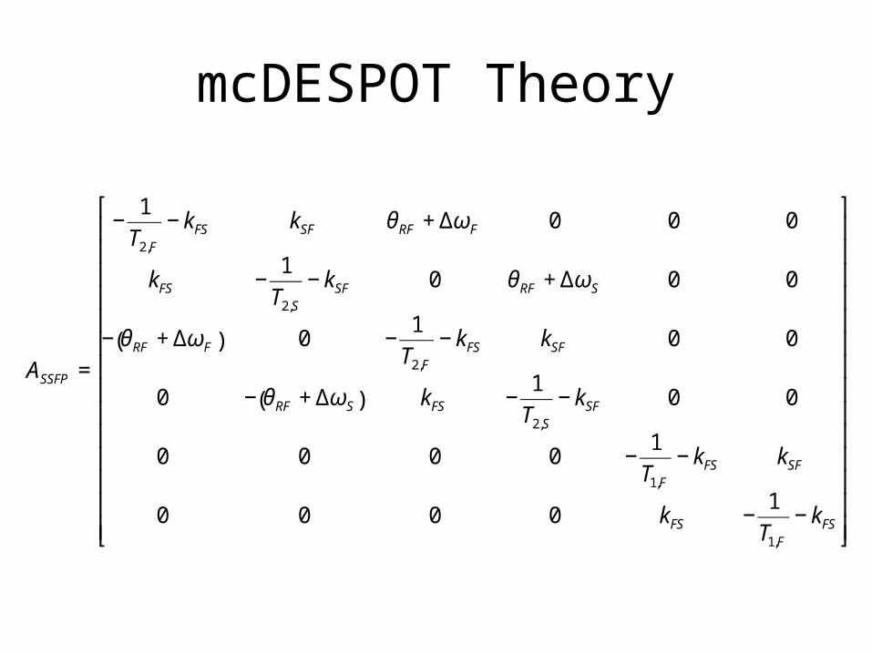
mcDESPOT Theory

€

ASSFP =

−1

T2,F

− kFS kSF θRF + ΔωF 0 0 0

kFS −1

T2,S

− kSF 0 θRF + ΔωS 0 0

− θRF + ΔωF( ) 0 −1

T2,F

− kFS kSF 0 0

0 − θRF + ΔωS( ) kFS −1

T2,S

− kSF 0 0

0 0 0 0 −1

T1,F

− kFS kSF

0 0 0 0 kFS −1

T1,F

− kFS

⎡

⎣

⎢ ⎢ ⎢ ⎢ ⎢ ⎢ ⎢ ⎢ ⎢ ⎢ ⎢ ⎢ ⎢ ⎢

⎤

⎦

⎥ ⎥ ⎥ ⎥ ⎥ ⎥ ⎥ ⎥ ⎥ ⎥ ⎥ ⎥ ⎥ ⎥

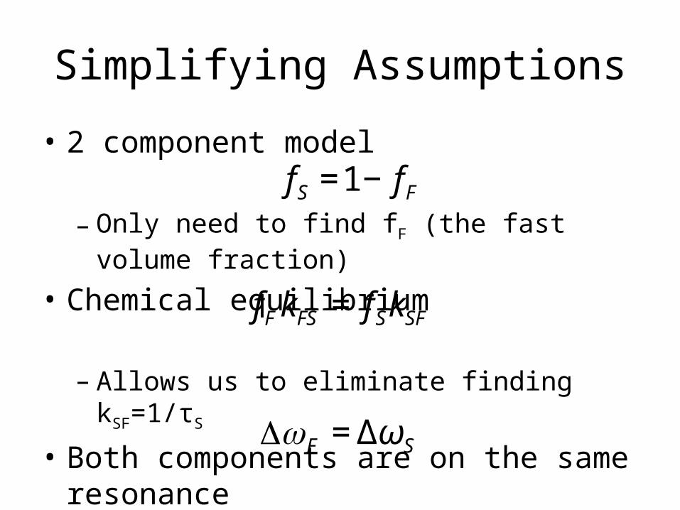
Simplifying Assumptions

• 2 component model

– Only need to find fF (the fast volume fraction)

• Chemical equilibrium

– Allows us to eliminate finding kSF=1/τS

• Both components are on the same resonance

€

fF kFS = fSkSF€

fS =1− fF

€

ΔωF = ΔωS

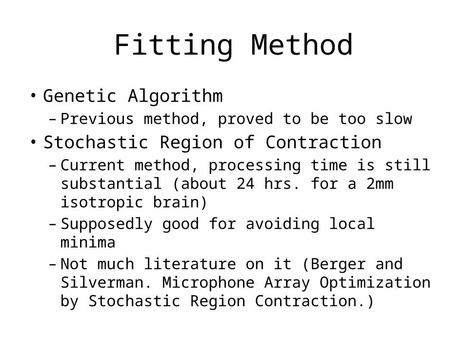
Fitting Method

• Genetic Algorithm– Previous method, proved to be too slow

• Stochastic Region of Contraction– Current method, processing time is still substantial

(about 24 hrs. for a 2mm isotropic brain)– Supposedly good for avoiding local minima– Not much literature on it (Berger and Silverman.

Microphone Array Optimization by Stochastic Region Contraction.)

Stochastic Region of Contraction

• Has been offered as an alternative to simulated annealing, which can be slow but is very general

• SRC is good for objective functions with these characteristics:– Few large valleys, many small local minima is fine– The neighborhood around the global minimum is

still lower than any other local minima– Depends on <100 variables

Stochastic Region of Contraction

• Given an initial N-dimensional, rectangular, search volume containing the global optimum– Explore the objective function with random points

in the space– Systematically contract the volume until it reaches

a satisfactorily small region that traps the global optimum

Stochastic Region of Contraction

• Algorithm– Define initial search space for: T1,F&S, T2,F&S, fF, τF, Δωs

– Treat this rectangular box as a uniform distribution and sample N times

– Compute the objective function for each sample– Keep M of the best samples and define the new

box based on the ranges of the variables in these samples

– Rinse and repeat until convergence

Stochastic Region of Contraction

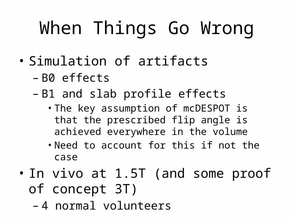
When Things Go Wrong

• Simulation of artifacts– B0 effects– B1 and slab profile effects• The key assumption of mcDESPOT is that the prescribed

flip angle is achieved everywhere in the volume• Need to account for this if not the case

• In vivo at 1.5T (and some proof of concept 3T)– 4 normal volunteers

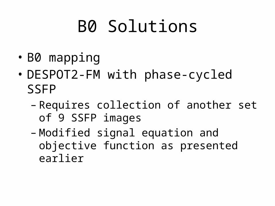
B0 Solutions

• B0 mapping• DESPOT2-FM with phase-cycled SSFP– Requires collection of another set of 9 SSFP

images– Modified signal equation and objective function as

presented earlier

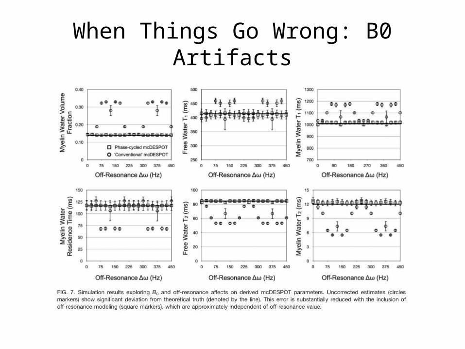
When Things Go Wrong: B0 Artifacts

When Things Go Wrong: B0 Artifacts

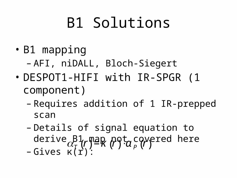
B1 Solutions

• B1 mapping– AFI, niDALL, Bloch-Siegert

• DESPOT1-HIFI with IR-SPGR (1 component)– Requires addition of 1 IR-prepped scan– Details of signal equation to derive B1 map not

covered here– Gives κ(r):

€

αT r( ) = κ r( ) ⋅α P r( )

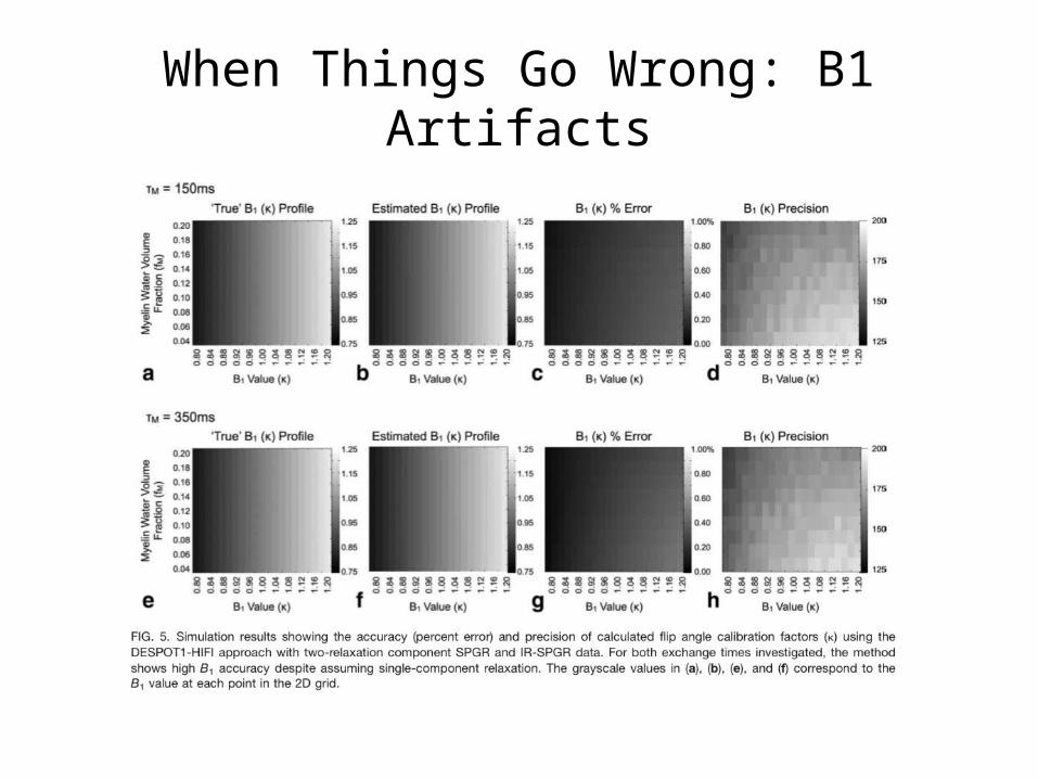
When Things Go Wrong: B1 Artifacts

When Things Go Wrong: B1 Artifacts

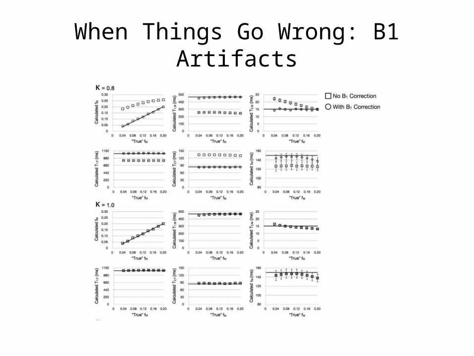
When Things Go Wrong: B1 Artifacts

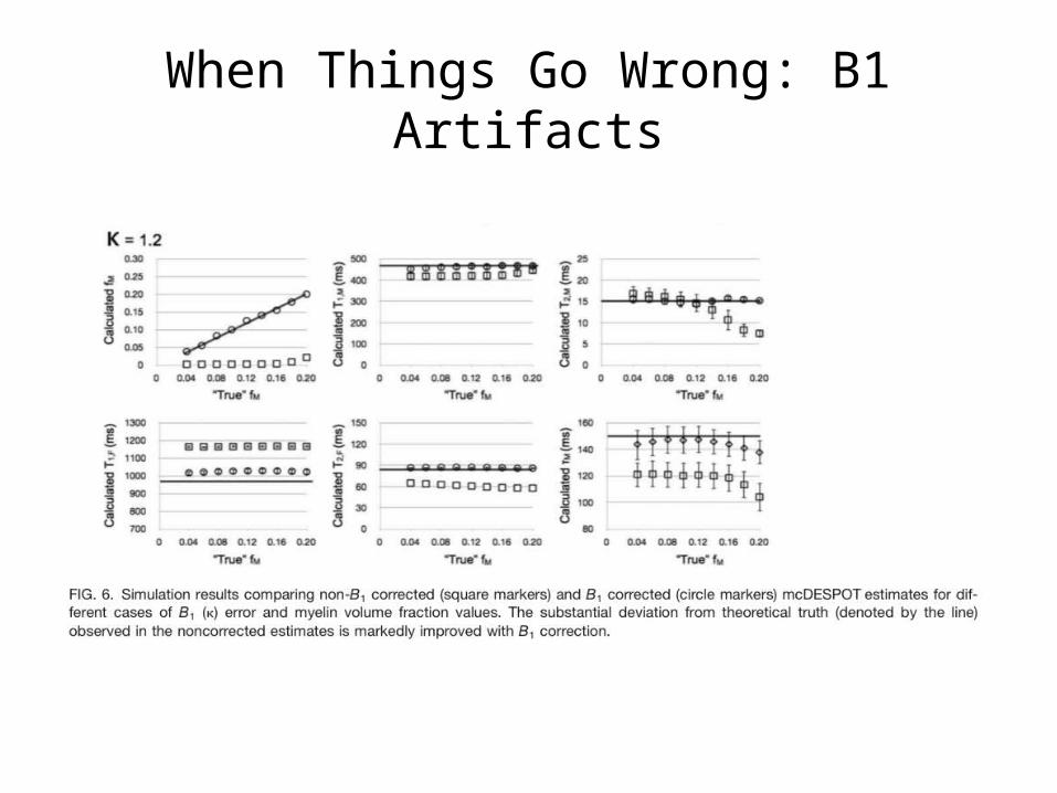
When Things Go Wrong: B1 Artifacts

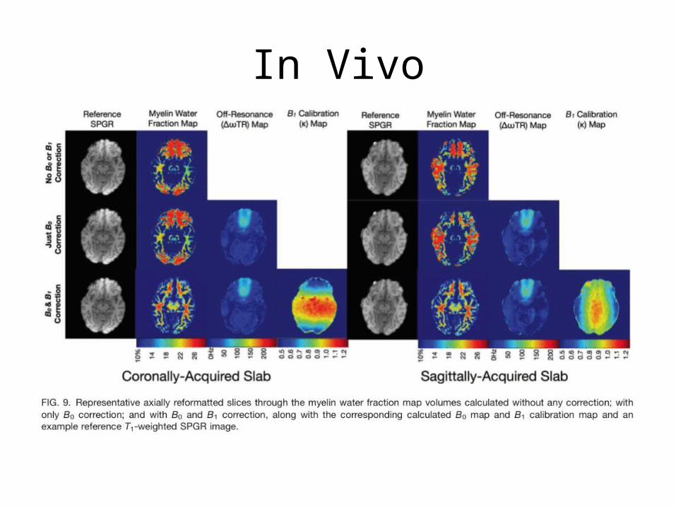
In Vivo

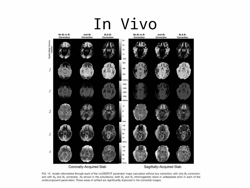
In Vivo

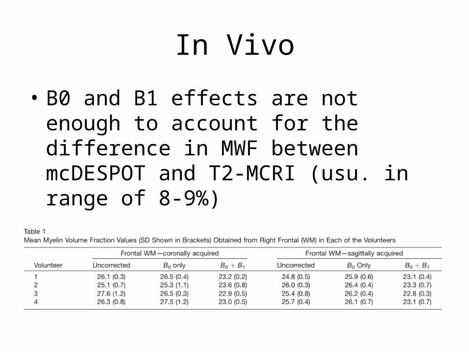
In Vivo

• B0 and B1 effects are not enough to account for the difference in MWF between mcDESPOT and T2-MCRI (usu. in range of 8-9%)

Conclusions

• DESPOT1-HIFI does well even thought slab profile changes with angle and assumes single component– Alternatives should be considered though since anatomical

structures are visible on the maps: not the best B1 map– Bloch-Siegert seems compelling but need a way to

incorporate slab profile as well• DESPOT2-FM and phase-cycled SSFP has been a part of

the protocol at 1.5T and should also stay when we move to 3T+– Alternative B0 mapping methods should be considered if

they offer a significant benefit in acquisition time

Other Avenues to Explore

• 3 component model, is another pool skewing the MWF?

• Are the 2 components actually on the same resonance?