Influence Chart for Vertical Stress Increases Due To Horizontal Shear Loadings RICHARD D. BARKSDALE and MILTON E. HARR

Respectively, University Fellow and Professor of Civil Engineering, Purdue University

An influence chart is presented for computing the vertical stress increase in the interior of a semi-infinite homogeneous isotropic elastic mass due to distributed horizontal shearing stresses applied at the surface. An example for a square surface area loaded with a uniform vertical stress and a wedge-shaped horizontal shearing stress is then worked out to illustrate the use of the influence chart. The mathematical development of the influence chart and a table summarizing the data required to construct the influence chart are also given.

•THE COMPUTATION of vertical stresses in a soil mass due to applied loadings is required for many problems in soil mechanics. Usually, as in the case of the con­solidation settlement of foundations, only the stress due to vertical loadings are com­puted, and the effects of any horizontal shear stress that may be developed between the foundation base and the soil are neglected. This paper presents a simple graphical method for computing the vertical stresses in the interior of a semi-infinite elastic mass due to distributed, horizontal shearing stresses applied at the surface.

As was done by Newmark (1) for vertical loadings, the vertical stresses duetohori­zontal shearing loads are determined by drawing the foundation to a proper scale, and then counting the number of squares that the load covers when superimposed on an in­fluence chart. Here also, the vertical stress is found by multiplying the horizontal shearing stress by the number of squares covered and a constant.

In the following sections the method of solution is presented, and an example is worked out illustrating the use of the influence chart. The detailed mathematical de­velopment of the influence chart and the data needed to construct the chart are given in the Appendix.

COMPUTATION OF VERTICAL STRESSES ON HORIZONTAL PLANES

The coordinate system used for the influence chart is shown in Figure 1. The x, y plane is taken as the horizontal surface of the semi-infinite soil mass, with the z axis extending vertically downward. Although any unidirectional distribution of horizontal shearing stress, qh, is permissible in the x, y plane, the directional orientation of the stress must be considered. This requirement, however, is not restrictive; it is meant only to demonstrate the applicability of this procedure in solving problems.

The influence chart (Fig. 2) is constructed to give the increase in normal stress, 6.uz, on a horizontal plane through point C ', vertically beneath point C (Fig. 1) due to a horizontal shear loading applied on the surface. The usual soil mechanics sign con­vention is to be used for t.az; a positive t.az stress change represents a compressive stress increase. As shown on Figures 1 and 2, horizontal shear loadings in quadrants 1 and 4 induce tensile t.az stresses at C ', and shear loadings in quadrants 2 and 3 cause compressive stresses.

Paper sponsored by Committee on Mechanics of Earth Masses and Layered Systems.

11

12

z.

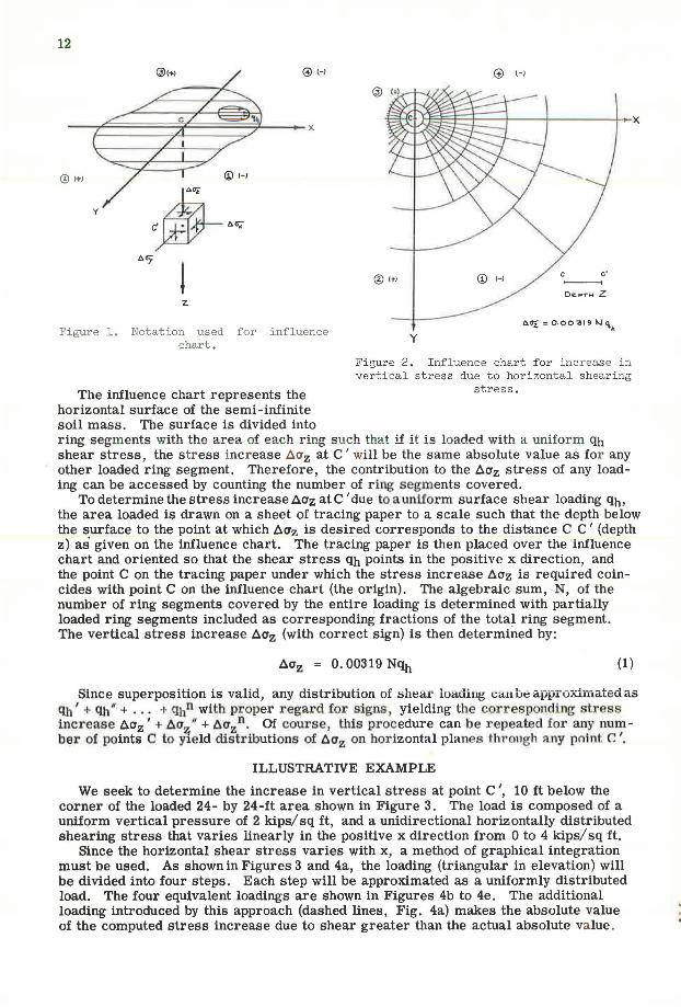
Figure 1. Notation used f or influence chart.

O.l'z: :0.00319 IJ<\~

y

Figure 2. Influence chart for increase in vertical stress du e t o horizontal shearing

The influence chart represents the horizontal surface of the semi-infinite soil mass. The surface is divided into

stress.

ring segments with the area of each ring such that if it is loaded with a uniform Cfu shear stress, the s tress incr ease l::.az at C 1 will be the same absolute value as for any other loaded ring segment. Therefore, the contribution to the l::.az stress of any load­ing can be accessed by counting the number of r ing segments covered.

To determine the stress increase /l.az at C 'due to a uniform surface shear loading %, the area loaded is drawn on a sheet of tracing paper to a scale such that the depth below the surface to the point at which t::.az is desired corresponds to the distance C C 1 (depth z) as given on the influence chart. The tracing paper is then placed over the influence chart and oriented so that the shear stress qh points in the positive x direction, and the point C on the tracing paper under which the stress increase l::.az is required coin­cides with point C on the influence chart (the origin). The algebraic sum, N, of the number of ring segments covered by the entire loading is determined with partially loaded ring segments included as corresponding fractions of the total ring segment. The vertical stress increase l::.az (with correct sign) is then determined by:

l::.az = 0. 00319 N% (1)

Since superposition is valid, any distribution of shear loading can be approximated as % ' + <lli w + ... + qhn with proper regard for s igns, yielding the corre13pondi ng stress increase l::.az' + Aa 11 + Aaz n. Of course, this procedure can be repeated for any num­ber of points C to y1eld distributions of llaz on horizontal planes th1·011gh :i. ny point C '.

ILLUSTRATIVE EXAMPLE

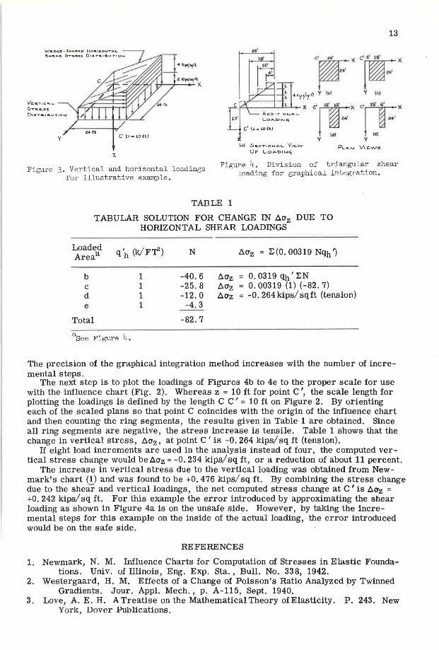
We seek to determine the increase in vertical stress at point C ', 10 ft below the corner of the loaded 24- by 24-ft area shown in Figure 3. The load is composed of a uniform vertical pressure of 2 kips/ sq ft, and a unidirectional horizontally distributed shearing stress that varies linearly in the positive x direction from 0 to 4 kips/ sq ft.

Since the horizontal shear stress varies with x, a method of graphical integration must be used. As shown in Figures 3 and 4a, the loading (triangular in elevation) will be divided into four steps. Each step will be approximated as a uniformly distributed load. The four equivalent loadings are shown in Figures 4b to 4e. The additional loading introduced by this approach (dashed lines, Fig. 4a) makes the absolute value of the computed stress increase due to shear greater than the actual absolute value .

W c.o.c;c- .sw ... ,.11:.0 Ho•1<L o w-r ... 1....

S w-:. .... a. ~T-.llC..llS 01~Ta. t ll. VT 10 ._.

y

4 klfo/~ll

c'lz ... io£t)

z (d) Sic.c.<10....i.o..1... View

Ov Lo ..... ou-1 <.j

13

Figure 3. Vertical and hori zontal l oadings for illustrative example .

Figure 4. Divis ion of triangular shear l oading for graphical integration.

TABLE 1

TABULAR SOLUTION FOR CHANGE IN t:i.az DUE TO HORIZONTAL SHEAR LOADINGS

Loaded q'h (k/FT2) Areaa

b 1 c 1 d 1 e 1

Total

aSee Figure 4.

N 6.az = 2::(0.00319 N%~

-40.6 -25.8

0. 0319 % I r:N 0. 00319 (1) (-82. 7)

-12.0 -0. 264 kips/ sq ft (tension) -4.3

-82.7

The precision of the graphical integration method increases with the number of incre­mental steps.

The next step is to plot the loadings of Figures 4b to 4e to the proper scale for use with the influence chart (Fig. 2). Whereas z = 10 ft for point C ', the scale length for plotting the loadings is defined by the length C C' = 10 ft on Figure 2. By orienting each of the scaled plans so that point C coincides with the origin of the influence chart and then counting the ring segments, the results given in Table 1 are obtained. Since all ring segments are negative, the stress increase is tensile. Table 1 shows that the change in vertical stress, 6.az, at point C' is -0. 264 kips/sq ft (tension).

If eight load increments are used in the analysis instead of four, the computed ver­tical stress change would be 6.az = -0. 234 kips/ sq ft, or a reduction of about 11 percent.

The increase in vertical stress due to the vertical loading was obtained from New­mark's chart (1) and was found to be +0. 476 kips/ sq ft. By combining the stress change due to the shear and vertical loadings, the net computed stress change at C' is 6.az = +0. 242 kips/ sq ft. For this example the error introduced by approximating the shear loading as shown in Figure 4a is on the unsafe side. However, by taking the incre­mental steps for this example on the inside of the actual loading, the error introduced would be on the safe side.

REFERENCES

1. Newmark, N. M. Influence Charts for Computation of Stresses in Elastic Founda­tions. Univ. of Illinois, Eng. Exp. Sta., Bull. No. 338, 1942.

2. Westergaard, H. M. Effects of a Change of Poisson's Ratio Analyzed by Twinned Gradients. Jour. Appl. Mech., p. A-115, Sept. 1940.

3. Love, A. E. H. A Treatise on the Mathematical Theory of Elasticity. P. 243. New York, Dover .Publications.

14

Appendix MATHEMATICAL DEVELOPMENT OF INFLUENCE CHART

The vertical stress increase ~az at any point C' (Fig. 5) in a semi-infinite homo­geneous isotropic elastic mass due to a concentrated horizontal surface loading~ was published in 1940 by Westergaard ~):

az 3~ 21TR2 cos ijJ sin 0 cos2 0 (2)

az 3~ x z" 21TR5 (3)

(According to A. E. H. Love (~), this problem received earlier attention by J. Bous­sinesq, V. Cerruti, and J. H. Mitchell.)

Of greater interest is the determination of the vertical stress increase at some depth z beneath point C (Fig. 6) due to a uniform horizontal shearing stress of

--r..r~~~...,..'"'7'"-r~----- x intensity qh, acting in the x direction over

T z

Figure 5. Notation used for determining vertical stress at point c' due to single

horizontal load QR.

y

IJOTC.:

'\.~ = ll>ITEN.SITY

OF" H02.lZONT.-..L.

L..0,.._0IN"i ( '"" )(,

D'R..ECTIOt..1)

Figure 6. Plan view of horizontal surface loading on small area.

part of a circular segment. The following expressions are apparent from Figure 6:

dAi = (pd¢) . dp (4)

d~ = % . dA1 - % (pd¢ dp) (5)

Substituting Eq. 5 into Eq. 3 gives for the differential of the vertical stress at some arbitrary constant depth z below C:

y

Pt...At-..1 Vcc.w

Figure 7. Notation used for Eq. 'Tb·

15

3 (pd¢ dp) (-p cos ¢) (z2) 27T • % [ JS

p2 cos2 ¢ + p2 sin2 ¢ + z2 r2 (6)

By simplifying and setting appropriate limits, we get:

I p= pf¢= ¢1 3 2 q p2 cos ¢ d¢ dp

az = - 27T z h [ J Bl P2 + z2 12

= Po ¢ = ¢0

(7a)

which after integration becomes:

% . . [( 1 )% ( 1 7'2 ] •z = - 2, [sm ¢, - sm ¢0) [' + (~.)'] - [' + (;;)']) (7b)

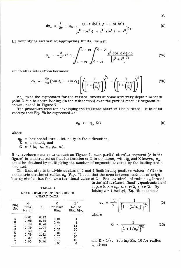
Eq. 7b is the expression for the vertical stress at some arbitrary depth z beneath point C due to shear loading (in the x direction) over the partial circular segment A, shown shaded in Figure 7.

The procedure used for developing the influence chart will be outlined. It is of ad­vantage that Eq. 7b be expressed as:

-% KG (8)

where

qh horizontal stress intensity in the x direction, K constant, and G f (z, ¢0, ¢1, Po, p1).

If everywhere over an area such as Figure 7, each partial circular segment (A in the figure) is constructed so that its fraction of G is the same, with iih and K known, az could be obtained by multiplying the number of segments covered by the loading and a constant.

The first step is to divide quadrants 1 and 4 (both having positive values of G) into concentric circles of radius an (Fig. 7) such that the area between each set of neigh­boring circles has the same fractional value of G. For any circle of radius an located

in the half surface defined by quadrants 1 and

Ring No.

A B c D E F G H

TABLE 2

DEVELOPMENT OF INFLUENCE CHART DATA

G G G' (total an for Each No. of

for an) Ring Ring Div.

0.01 0.22 0.01 1 0.05 0.40 0.19 0.70 0.04 4

0.39 1. 07 0.14 14

0.59 1. 54 0.20 20

0. 79 2.42 0.20 20

0.89 3.52 0. 20 20

0.95 5. 36 0. 10 10 0.06 6

4, po=O, p1=an, ¢o=-1T/2, ¢1=1T/2. By letting z = 1 (unity), Eq. 7b becomes:

(9)

G 1 (10)

and K = 1/ 1T. Solving Eq. 10 for radius an gives:

16

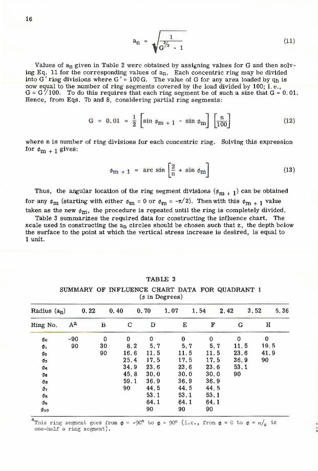
(11)

Values of an given in Table 2 were obtained by assigning values for G and then solv ­ing Eq. 11 for the corresponding values of an. Each concentric ring may be divided into G' ring divisions where G' = 100 G. The value of G for any area loaded by~ is now equal to the number of ring segments covered by the load divided by 100; i.e., G = G './ 100. To do this requires that each ring segment be of such a size that G = 0. 01. Hence, from Eqs. 7b and 8, considering partial ring segments:

G = 0.01 = i [sin ~+ 1 - sin ¢m] [1 ~0] (12)

where n is number of ring divisions for each concentric ring. for ¢m + 1 gives:

Solving this expression

. [2 . ] lllm + 1 = arc sin n + sm <l>m (13)

Thus, the angular location of the ring segment divisions (¢m + 1) can be obtained

for -any ¢m (starting with either ¢m = 0 or ¢m = -TT/2). Then with this ¢m + 1 value taken as the new ¢m, the procedure is repeated until the ring is completely divided.

Table 3 summarizes the required data for constructing the influence chart. The scale used in constructing the an circles should be chosen such that z, the depth below the surface to the point at which the vertical stress increase is desired, is equal to 1 unit.

TABLE 3

SUMMARY OF INFLUENCE CHART DATA FOR QUADRANT 1 (¢ in Degrees)

Radius (an) 0.22 0.40 0.70 1. 07 1. 54 2.42 3. 52

Ring No. Aa B c D E F G

¢0 -90 0 0 0 0 0 0 ¢1 00 30 8.2 5.7 5.7 5.7 11. 5 </i2 90 16.6 11. 5 11. 5 11. 5 23.6 Q\3 25.4 17.5 17.5 17.5 36.9 ¢4 34.9 23.6 23.6 23. 6 53.1 Ills 45. 8 30. 0 30.0 30.0 90 Ille 59.1 36 . 9 36.9 36.9 Q\7 90 44.5 44 . 5 44 . 5 Ille 53.1 53.1 53.1 Ille 64 . 1 64. 1 64 . 1 ¢10 90 90 90

5.36

H

0 19. !l 41. 9 90

aThis ring segment goes f r om ¢ = -90° to ¢ = 900 ( i.e .' f r om ¢ = 0 to Ill = n/2 is

one- hal f a ring segment) .

17

From Eq. 7b it follows that loadings in quadrants 1 and 4 induce negative vertical stresses and loadings in quadrants 2 and 3 correspond to positive vertical stresses. Recognizing that symmetry with respect to both the x and y axes is preserved, the tabulated data in Table 3 are sufficient to construct the entire influence chart wherein the vertical stress increase is given by:

(14)

where N is the algebraic sum of the segments covered by the horizontal loading.

Discussion E. S. BARBER, Consulting Engineer, Soil Mechanics and Foundations-The paper is clearly presented and the chart is useful. However, a similar chart was already available. As been pointed out by the writer (4), the vertical stress from a shear load is the same as the shear stress from a verticai load. Therefore, Newmark's Figure 5 (1) is the same as the authors' chart except that Newmark's figure has finer divisions wifh a more convenient influence value of 0. 001.

There is a similar correspondence between the shear stress from a shear load and the parallel horizontal normal stress (for Poisson's ratio equal to 0. 5) from a normal load. Influence charts for horizontal normal stresses from a shear load are presented in the June 1965 issue of Public Roads.

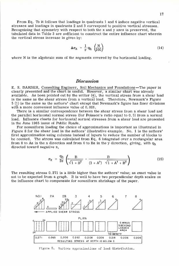
For nonuniform loading the choice of approximations is important as illustrated in Figure 8 for the shear load in the authors' illustrative example. No. 1 is the authors' first approximation using columns instead of layers to reduce the number of blocks to be counted. The stress was calculated from Eq. 6 integrated over a rectangular area from 0 to Az in the x direction and from 0 to Bz in the y direction, giving, with % directed toward negative x,

O'z (15)

The resulting stress 0. 271 is a little higher than the authors' value; an exact value is not to be expected from a graph. It is well to have two perpendicular depth scales on the influence chart to compensate for nonuniform shrinkage of the pape·r.

2A 28

--- APPLIED SHEAR STRESS

PLAN

DWITJ

7 8

LJ

D 6MINUS D 5 BEYOND LOADED

AREA

TOINFINTY

0 .27 I 0.065 0 .206 0.262 0 .2 06 0.209 0.216 0.206 0.206

RESULTING STRESS AT DEPTH 10 BELOW C

Figure 8. Va rious approx lluaLlom; ur loa d distribution.

18

To make the total load of the approximation the same as the load to be approximated, No. 2A of Figure 8 is subtracted from No. 1 to obtain No. 2B. The resulting stress O. 206 is the same as No. 8 obtained by exact integration. For a stress increasing from 0 at x = 0 to % at x = Az:

% (11 B C1z = 211 4A - (l + A2) ~l + A2 + B2

1 . -1 A2

B2

- 1 - A2

- B2) + -sin

2A A2 B2 + 1 + A2 + B2 (16)

No. 3 is an unsatisfactory approximation but Nos. 4 and 5 are good. No. 4 balances over and under approximations and requires only two areas. No. 5· uses a single area with the centroid at the same location as the load to be approximated. No. 6 shows the small effect, in this case, of extending the loaded area to infinity.

Reference

4. Barber, E. S. Application of Triaxial Compression Test Results to the Calcula­tion of Flexible Pavement Thickness. Highway Research Board Proc., Vol. 26, p. 37, 1946.

R. D. BARKSDALE and M. E. HARR, Closure-The authors thank Mr. Barber for pointing out that influence charts for computing the verticat stress at a point from a shear load on the surface are the same as those for computing the horizontal shear stress from a vertical load. This correspondence is implied by the Maxwell-Betti reciprocal theorem (5) since the semi-infinite solid is assumed to be elastic and fol­lows Hooke's law. -

The manner in which the load is approximated is certainly important in obtaining an accurate answer, as pointed out by Mr. Barber. The authors realized that the ap­proximation used in the example would give an answer slightly on the high side and pointed this out in the discussion. The main purpu~e uI the example was to illustrate the use of the chart and a simple numerical method of integration which could be applied to any load distribution.

Reference

5. Norris, C. H., and Wilbur, J. B. Elementary Structural Analysis. P. 390. New York, McGraw-Hill, 1960.