IMPLEMENTATION AND EVALUATION OF A

MULTIBAND OFDM ULTRA WIDE BAND SYSTEM

By SWAMINATHAN DURAISAMY

A thesis submitted to the

Graduate School-New Brunswick

Rutgers, The State University of New Jersey

in partial fulfillment of the requirements

for the degree of

Master of Science

Graduate Program in Electrical and Computer Engineering

written under the direction of

Prof. Predrag Spasojevic

and approved by

New Brunswick, New Jersey

May, 2013

© 2013

Swaminathan Duraisamy

ALL RIGHTS RESERVED

ii

ABRACT OF THE THESIS

Implementation and Evaluation of a Multiband OFDM

Ultra Wide Band System

by Swaminathan Duraisamy

Thesis Director: Prof. Predrag Spasojevic

WPAN systems have been receiving significant attention from both industry and

academia in the last 10 years and Ultra Wide Band (UWB) technology is one among

them. Nowadays, UWB systems can transmit at a data rate as high as 500 Mbps for short

distances consuming very little power. When a UWB system moves from the laboratory

environment to a real world scenario, several design issues are encountered such as

complexity, power consumption, cost and flexibility. In this thesis, a UWB system is

designed using a Multiband OFDM physical layer approach which tackles the problems

mentioned above while still ensuring high data rates with less power consumption. The

reason for choosing this approach over a traditional spread spectrum approach is that the

system sends the signal on several sub-bands one at a time making it spectrally flexible

while using lesser bandwidth and, hence, preventing the need for high speed RF circuits

and ADC’s. This will reduce the design complexity and, thereby, reducing the power

consumption and making this technology a low cost solution. Since the information on

iii

each of these bands uses a multicarrier (OFDM) technique, this system inherits several

nice properties of OFDM such as high spectral efficiency, resilience to RF interference,

robustness to multi-path, and the ability to efficiently capture multi-path energy.

This thesis focuses on optimizing the Bit Error Rate (BER) performance of the

system by making use of symbol diversity and multicarrier diversity techniques. Symbol

diversity is implemented by sending an OFDM symbol on different sub-bands and

improve the BER by combining the outputs using Maximal Ratio Combining. In

multicarrier diversity, the performance is improved further by sending the same data on

different subcarriers in an OFDM signal. In addition, a study of the performance by

sending the data sensibly on different subcarriers in an OFDM symbol using prior

channel information is conducted. The various blocks needed to design the transmitter

chain and the receiver chain of the system were implemented using a LabVIEW software

testbed and a frequency selective fading channel suggested by the UWB standards

committee was simulated to study the performance of the system.

iv

List of Figures

2.1. Frequency spectrum of an OFDM signal ................................................................. 3

2.2. MB-OFDM frequency band of operation ................................................................ 4

2.3. Symbol timing of OFDM symbols on different bands ............................................. 5

3.1. Preamble sequence for an OFDM frame .................................................................. 9

3.2. Constellation points for QPSK modulation ............................................................ 11

3.3. Cyclic Prefix of an OFDM symbol ........................................................................ 13

4.1. Block diagram of an MB-OFDM transmitter ......................................................... 14

4.2. Block diagram of an OFDM receiver .................................................................... 16

4.3. Parallel auto-correlator structure ........................................................................... 17

4.4. An illustration on the Autocorrelation Structure based TFC identification via

Band switching .................................................................................................... 18

4.5. Timing metric obtained by correlating 2 preamble symbols together .................... 19

4.6. Structure of an iterative Carrier Frequency Offset (CFO) estimator ...................... 21

4.7. Pilot subcarriers arrangement in an OFDM symbol .............................................. 22

4.8. Maximal Ratio Combiner ..................................................................................... 23

4.9. Front panel view of Modulation parameters control in LabVIEW ......................... 25

4.10. Front panel view of Channel parameters control in LabVIEW .............................. 25

4.11. Frequency spectrum of UWB channel for different values of n ........................... 28

4.12. Impulse response of UWB channel for different bands ......................................... 30

v

5.1. BER vs SNR curve for the system in an AWGN channel with Noise

Variance N0=0.01 ................................................................................................. 31

5.2. Channel frequency spectrum showing the frequencies on which same data

is sent not knowing/knowing the channel information in advance ......................... 33

5.3. Channel frequency spectrum showing the frequencies on which same data is sent

not knowing the channel information in advance .................................................. 35

5.4. Channel frequency spectrum showing the frequencies on which same data is sent

knowing the channel information in advance ........................................................ 38

5.5. BER curves showing the performance in a UWB channel using an equalizer,

symbol diversity and multicarrier diversity ........................................................... 40

5.6. BER curves showing the performance in a UWB channel for different values

of N ..................................................................................................................... 41

vi

List of Tables

3.1. Bits – Symbol mapping for QPSK........................................................................... 11

3.2. Time Frequency Code for the band allocation of OFDM symbols ........................... 12

4.1. Simulation parameters ............................................................................................ 24

vii

Acknowledgements

I would like to express my sincere gratitude to my advisor Prof. Predrag Spasojevic

whose guidance helped me a lot at every phase of the project. I would like to thank my

family for their constant support throughout the course of the project. I would also like to

thank Prof. David Daut and Prof. Zoran Gajic for supervising my thesis defense.

A major reason for my motivation to do a thesis was the project which we worked on as a

part of the Digital Communication Systems course under Prof. Predrag Spasojevic. The

laboratory sessions on USRP Software Defined Radio conducted by the course TA,

Swapnil Mhaske, and the interactions with my project partner Chun-Ta Kung on the

practical implementation of a communication system helped me to understand many of

the conceptual details and greatly benefitted my research.

Finally, I am indebted to my friends for their invaluable support during the course of

graduate study.

viii

Dedication

To my parents, teachers and friends

ix

Table of Contents

Abstract ......................................................................................................................... ii

List of Figures .............................................................................................................. iv

List of Tables ................................................................................................................ vi

Acknowledgements ......................................................................................................vii

Dedication .................................................................................................................. viii

1. Introduction ............................................................................................................ 1

2. Background .............................................................................................................. 3

2.1. OFDM ................................................................................................................ 3

2.2. MB-OFDM UWB ............................................................................................... 4

2.2.1. Advantages ............................................................................................... 5

3. Physical Layer Specifications and Features ............................................................ 8

3.1. Mathematical Representation of a UWB signal .................................................. 8

3.2. Preamble Sequence ............................................................................................ 9

3.3. Subcarrier Constellation Mapping ..................................................................... 10

3.4. Time domain spreading .................................................................................... 11

3.5. Cyclic Prefix Insertion ..................................................................................... 12

4. System Design ....................................................................................................... 14

4.1. Transmitter ...................................................................................................... 14

4.1.1. Source ................................................................................................... 14

4.1.2. Modulation ............................................................................................ 14

4.1.3. IFFT ...................................................................................................... 15

x

4.1.4. Diversity/Multicarrier Diversity .............................................................. 15

4.1.5. TFC allocation ........................................................................................ 16

4.2. Receiver .......................................................................................................... 16

4.2.1. Synchronization ..................................................................................... 17

4.2.2. FFT ....................................................................................................... 22

4.2.3. Channel Estimation ............................................................................... 22

4.2.4. Equalizer ............................................................................................... 23

4.2.5. Diversity ................................................................................................ 23

4.3. Simulation ........................................................................................................ 24

4.4. Simulation Front Panel ..................................................................................... 25

4.5. Channel .......................................................................................................... 26

4.5.1. AWGN Channel .................................................................................... 26

4.5.2. UWB Channel ....................................................................................... 26

5. Experiments and Results ........................................................................................ 31

5.1. Experimental Setup for BER performance in an AWGN channel .................... 31

5.2. Experimental Setup for a system with/without diversity .................................. 32

5.3. Effect of multipath components ....................................................................... 39

5.4. Effect of n ..................................................................................................... 40

6. Conclusion and Future Direction .......................................................................... 42

6.1. Conclusion ....................................................................................................... 42

6.2. Future Work ..................................................................................................... 43

References .................................................................................................................... 44

1

Chapter 1

Introduction

ULTRAWIDEBAND (UWB) communication technology is emerging as a leading

standard for high-data-rate applications over wireless networks. Due to its use of a high-

frequency bandwidth, UWB can achieve very high data rates over the wireless

connections of multiple devices at a low transmission power level close to the noise floor.

In this order, the FCC allocated the spectrum from 3.1 to 10.6 GHz for unlicensed use by

UWB transmitters operated at a limited transmission power of −41.25 dBm/MHz or less.

Since the power level allowed for UWB transmissions is considerably low, UWB devices

will not cause significantly harmful interference to other communication standards.

A significant difference between conventional radio transmissions and UWB is that

conventional systems transmit information by varying the power level, frequency, and/or

phase of a sinusoidal wave whereas UWB transmissions transmit information by

generating radio energy at specific time intervals and occupying a large bandwidth, thus

enabling pulse-position or time modulation. The wide bandwidth and potential for low-

cost digital design enable a single system to operate in different modes as a

communications device, radar, or locator. These properties give UWB systems a clear

technical advantage over other conventional approaches in high multipath environments

at low to medium data rates.

The IEEE 802.15.3a High Rate Alternative Physical Layer (PHY) Task Group

(TG3a) for Wireless Personal Area Networks (WPAN) has been established to

standardize the development of UWB devices. IEEE 802.15.3a task group which deals

2

with high data rate WPAN applications came up with 2 PHY layer proposals: 1) Multi-

band OFDM UWB (MB-OFDM) and 2) Direct Sequence UWB (DS-UWB). The

orthogonal frequency-division multiplexing (OFDM)-based physical layer is one of the

most promising options for the PHY due to its capability to capture multipath energy and

eliminate inter-symbol interference. Despite the aforementioned merits, the extremely

short range, e.g., 10 m for a data rate of 110 Mb/s, puts UWB at an obvious disadvantage

when compared to other competitive technologies, such as the soon coming IEEE

802.11n standard, which supports a data rate of 200 Mb/s for 40 m in indoor

environments.

3

Chapter 2

Background

2.1 OFDM

Orthogonal frequency-division multiplexing (OFDM) is a method of encoding digital

data on multiple carrier frequencies. The data are sent over parallel sub-channels with

each sub-channel modulated by a modulation scheme such as BPSK, QPSK, 16 QAM

etc. The advantage of OFDM is its ability to cope with severe channel conditions

compared to a single carrier modulation scheme but still maintaining the data rates of a

conventional scheme with the same bandwidth. Furthermore, channel equalization is

simplified because OFDM may be viewed as using many slowly modulated narrow

band signals rather than one rapidly modulated wide band signal. Also, the low symbol

rate naturally makes the use of guard interval between symbols reducing ISI. Orthogonal

Frequency Division Multiplexing has become one of the mainstream physical layer

techniques used in modern communication systems.

Figure 2.1: Frequency spectrum of an OFDM signal.

2.2 MB-OFDM UWB

4

MB-OFDM UWB transmits data simultaneously over multiple carriers spaced apart

at precise frequencies on more than one band. OFDM signal needs precisely overlapping

but non-interfering carriers, and achieving this precision requires the use of a real-time

Fourier transform, which became feasible with improvements in Very Large-Scale

Integration (VLSI). Basically, MB-OFDM system provides time-domain diversity by

time-domain symbol spreading technique and frequency-domain diversity by transmitting

OFDM symbols in different sub-bands. Fast Fourier Transform algorithms provide nearly

100 percent efficiency in capturing energy in a multi-path environment, while only

slightly increasing transmitter complexity. Beneficial attributes of MB-OFDM include

high spectral flexibility and resiliency to RF interference and multi-path effects. Although

a wide band of frequencies could be used from a theoretical viewpoint, certain practical

considerations limit the frequencies that are normally used for MB-OFDM UWB.

Limiting the upper bound simplifies the design of the radio and analogue front end

circuitry as well as reducing interference with other services.

Figure 2.2: MB-OFDM frequency band of operation.

5

Figure 2.3: Symbol timing of OFDM symbols on different bands

An example of how the OFDM symbols are transmitted in a multi-band OFDM

system is shown in figure 2.2. The first OFDM symbol is transmitted on channel number

1 (3168MHz ~ 3696MHz), the second OFDM symbol is transmitted on channel number 3

(4224MHz ~ 4752MHz), the third OFDM symbol is transmitted on channel number

2(3696MHz ~ 4224MHz), the fourth OFDM symbol is transmitted on channel number 1

(3168MHz ~ 3696MHz), and so on.

2.2.1 Advantages

Multipath Robustness

An OFDM system offers inherent robustness to multi-path dispersion with a low-

complexity receiver. Adding a Cyclic Prefix (CP) forces the linear convolution with the

channel impulse response to resemble a circular convolution. A circular convolution in

the time domain is equivalent to a multiplication operation in the frequency domain.

Hence, a one-tap frequency domain equalizer is sufficient to undo the effect of the multi-

6

path channel. Any multi-path energy outside the CP window would result in inter-carrier-

interference (ICI). The length of the CP determines the amount of captured multi-path

energy and its length should be chosen to minimize the performance degradation due to

the loss in collected multi-path energy and the resulting ICI, while still keeping the CP

overhead small.

Tone allocation

Increasing the number of tones in an OFDM system decreases the overhead due to

CP. On the other hand, the complexity of the Fast Fourier transform/inverse Fast Fourier

transform (FFT/IFFT) block increases and the spacing between adjacent tones decreases.

We need to provide the best tradeoff between the CP overhead and FFT complexity. In

this system, we use 128 tones. To be compliant with FCC regulation, the 10-dB

bandwidth of an UWB signal should be at least 500 MHz and this implies the use of at

least 122 tones. Hence, the 128 tones are partitioned into 100 data tones, 22 pilot tones

and 6 null tones.

Complexity/Power Consumption

Multiband OFDM system has been specifically designed to be a low complexity

solution. By limiting the transmitted symbols to a quadrature phase-shift keying (QPSK)

constellation, the resolution of the DAC/ADC and the internal precision in the digital

baseband, especially the FFT, can be lowered. This system's lower complexity is also due

to the relatively large spacing between the carriers when compared to an IEEE 802.11a

system. This large spacing relaxes the phase noise requirements on the carrier synthesis

circuitry and improves robustness to synchronization errors. Multiband OFDM has

7

decided advantages over other possible implementations of UWB in terms of the

simplicity as well as the efficiency of its multi-path energy capture.

Interference Mitigation

Interference mitigation can be achieved by avoiding a certain part of the spectrum.

Since the bandwidth of other technologies such as Bluetooth and 802.11 which act as

interferers is very less, it will interfere with only a couple of tones in an OFDM signal.

The affected tones can be either erased, or the data rate of the affected tones should be

reduced to combat narrow-band interference on the UWB signal. To compensate for the

loss in performance, the data rate of the unaffected tones can be increased to a higher data

rate. The sub-band in which the narrowband interferer is present can still be used with

minimal impact. Frequency hopping also improved the coexistence ability with other

technologies by averaging out the aggregating interference.

8

Chapter 3

Physical Layer Specifications and Features

3.1 Mathematical Representation of a UWB signal

The transmitted signals can be described using a complex baseband signal notation. The

actual RF transmitted signal is related to the complex baseband signal as follows:

Where,

Re() represents the real part of a complex variable

rk(t) is the complex baseband signal of the kth OFDM symbol and is nonzero over

the interval from 0 to TSYM

N is the number of OFDM symbols

TSYM is the symbol interval and TSYM = TFFT + TCP

fk(mod)3 is the center frequency for the k(mod)3 band.

The parameters f and NST are defined as the subcarrier frequency spacing and the

number of total subcarriers used, respectively. Cn is the complex symbol sent on the

subcarrier frequency and the resulting waveform has a duration of TFFT = 1/ f. Shifting

the time by TCP creates the “circular prefix” which is used in OFDM to mitigate the

effects of multipath.

9

3.2 Preamble Sequence

The standard PLCP preamble, which is shown in the Figure 3.1, consists of three

distinct portions: packet synchronization sequence, frame synchronization sequence, and

the channel estimation sequence.

Figure 3.1: Preamble sequence for an OFDM frame.

The packet synchronization sequence shall be constructed by successively

appending 21 periods, denoted as {PS0, PS1, …, PS20 }, of a time-domain sequence. Each

period of the timing synchronization sequence shall be constructed by pre-appending 32

“zero samples” and by appending a guard interval of 5 “zero samples” to the sequences.

This portion of the preamble can be used for packet detection and acquisition, coarse

carrier frequency estimation, and coarse symbol timing.

10

Similarly, the frame synchronization sequence shall be constructed by successively

appending 3 periods, denoted as {FS0, FS1, FS2}, of an 180 degree rotated version of the

time-domain sequence. Again, each period of the frame synchronization sequence shall

be constructed by pre-appending 32 “zero samples”. This portion of the preamble can be

used to synchronize the receiver algorithm within the preamble. Finally, the channel

estimation sequence shall be constructed by successively appending 6 periods of the

OFDM training symbol, denoted as {CE0, CE1, …,CE5}. Packet synchronization

sequences and frame synchronization sequences have been specified in time domain and

channel estimation sequence in frequency domain by the UWB standards committee.

Different types of preambles have been designed to operate in four different

environments and they are:

Preamble 1 for Line Of Sight (LOS) (0–4 m)

Preamble 2 for Non Line Of Sight (NLOS) (0–4 m)

Preamble 3 for Non Line Of Sight (4-10 m)

Preamble 4 for extreme Non Light Of Sight

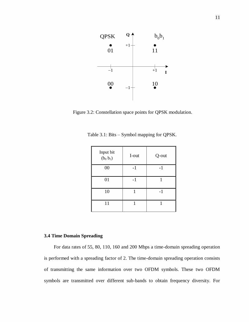
3.3 Subcarrier Constellation Mapping

The OFDM subcarriers shall be modulated using QPSK modulation. The serial input

data shall be divided into groups of 2 bits and converted into complex numbers

representing QPSK constellation points. The conversion shall be performed according to

the constellation mappings that employ a Gray-coded method.

11

+11

+1

1

Q

I

QPSK

01 11

b0b

1

00 10

Figure 3.2: Constellation space points for QPSK modulation.

Table 3.1: Bits – Symbol mapping for QPSK.

3.4 Time Domain Spreading

For data rates of 55, 80, 110, 160 and 200 Mbps a time-domain spreading operation

is performed with a spreading factor of 2. The time-domain spreading operation consists

of transmitting the same information over two OFDM symbols. These two OFDM

symbols are transmitted over different sub-bands to obtain frequency diversity. For

Input bit

(b0 b1) I-out Q-out

00 -1 -1

01 -1 1

10 1 -1

11 1 1

12

example, if the device uses a time-frequency code [1 2 3 1 2 3], as specified in table 3.2,

the information in the first OFDM symbol is repeated on sub-bands 1 and 2, the

information in the second OFDM symbol is repeated on sub-bands 3 and 1, and the

information in the third OFDM symbol is repeated on sub-bands 2 and 3. Time-frequency

code (TFC) determines the band on which every OFDM symbol has to be sent.

Table 3.2: Time Frequency Code for the band allocation of OFDM symbols.

3.5 Cyclic Prefix Insertion

Zero padded cyclic prefix refers to the prefixing of a symbol with zero samples.

Although the receiver is typically configured to discard the cyclic prefix samples, the

cyclic prefix serves two purposes.

It allows the linear convolution of a frequency-selective multipath channel to be

modeled as circular convolution, which in turn may be transformed to the frequency

domain using a discrete Fourier transform. This approach preserves orthogonality

between the subcarriers in an OFDM symbol and allows for simple frequency-domain

processing such as channel estimation and equalization.

Preamble

pattern Time Frequency Code (TFC)

1 1 2 3 1 2 3

2 1 3 2 1 3 2

3 1 1 2 2 3 3

4 1 1 3 3 2 2

13

As a guard interval, it eliminates the intersymbol interference (ISI) from the previous

symbol.

In order for the cyclic prefix to be effective, the length of the cyclic prefix must

be at least equal to the length of the multipath channel.

Figure 3.3: Cyclic Prefix of an OFDM symbol.

14

Chapter 4

System Design

4.1 TRANSMITTER

Figure 4.1: Block Diagram of an MB-OFDM Transmitter.

4.1.1 SOURCE

We used a PN sequence generator to generate a random bit stream. The output is a

1-dimensional array of bits. We then perform a serial-to-parallel conversion sending the

bits on parallel streams each representing a subcarrier.

4.1.2 MODULATION

We used the QPSK modulation scheme on all the subcarriers. We also have the

option of using multicarrier diversity by sending the same bit stream on two different

subcarriers.

4.1.3 IFFT

15

We then perform the IFFT of all the parallel data streams together ensuring

orthogonality between the subcarriers and the conversion of symbols to time domain. By

orthogonality, it is meant that all the subcarriers on which the data has been sent overlap

each other in such a way that they don’t interfere with one another and ensure minimum

bandwidth usage. IFFT for a set of N complex data points from N orthogonal parallel

streams is given by the formula.

; (n=0,1,….N-1) (4.1)

Where,

X(k) is a complex frequency domain data sent on subcarriers of frequency k/N,

k=0,1,….,N

k/N term is orthogonal to every other value of k/N

4.1.4 DIVERSITY/ MULTICARRIER DIVERSITY:

Before sending a signal through the transmitter antenna, we have an option to

increasing the BER performance by sending the same signal on different bands or

sending the data on multiple subcarriers within an OFDM symbol. When we have more

than one copy of the transmitted data i.e. the whole symbol or individual subcarriers of a

symbol, we can use a diversity scheme like Maximal Ratio Combining and obtain a lower

BER for the same SNR.

4.1.5 TFC ALLOCATION:

After inserting the Cyclic Prefix to all the symbols, we send the symbols on one of

the three bands based on time frequency code (TFC). Every TFC corresponds to a

16

specific preamble sequence which in turn corresponds to the type of environment. We

can improve the performance by sending the symbol on 2 different bands and make use

of diversity schemes like Maximal Ratio Combining at the receiver.

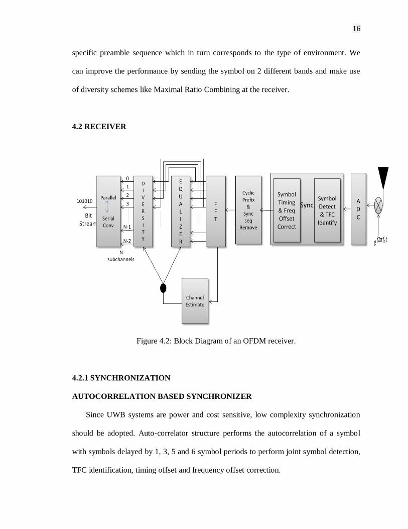
4.2 RECEIVER

Figure 4.2: Block Diagram of an OFDM receiver.

4.2.1 SYNCHRONIZATION

AUTOCORRELATION BASED SYNCHRONIZER

Since UWB systems are power and cost sensitive, low complexity synchronization

should be adopted. Auto-correlator structure performs the autocorrelation of a symbol

with symbols delayed by 1, 3, 5 and 6 symbol periods to perform joint symbol detection,

TFC identification, timing offset and frequency offset correction.

17

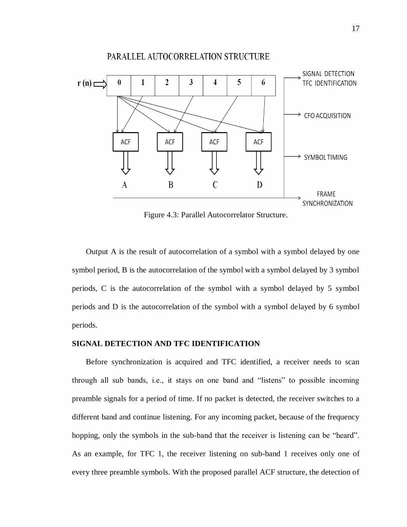
Figure 4.3: Parallel Autocorrelator Structure.

Output A is the result of autocorrelation of a symbol with a symbol delayed by one

symbol period, B is the autocorrelation of the symbol with a symbol delayed by 3 symbol

periods, C is the autocorrelation of the symbol with a symbol delayed by 5 symbol

periods and D is the autocorrelation of the symbol with a symbol delayed by 6 symbol

periods.

SIGNAL DETECTION AND TFC IDENTIFICATION

Before synchronization is acquired and TFC identified, a receiver needs to scan

through all sub bands, i.e., it stays on one band and “listens” to possible incoming

preamble signals for a period of time. If no packet is detected, the receiver switches to a

different band and continue listening. For any incoming packet, because of the frequency

hopping, only the symbols in the sub-band that the receiver is listening can be “heard”.

As an example, for TFC 1, the receiver listening on sub-band 1 receives only one of

every three preamble symbols. With the proposed parallel ACF structure, the detection of

18

signal is declared immediately once the ACF outputs (after comparing to a given

threshold) matches the ones given in the figure 4.4.

Figure 4.4: An illustration on the Autocorrelation Structure based TFC

identification via band switching.

Figure 4.4 shows the correlation peaks when the listener listens to band 1 for a

duration of 7 symbol periods and then listens to band 2 for the same duration. The output

pattern of the signal detector is assumed to be [0 1 0 1] (B=1, D=1) and the possible TFC

is either 1 or 2. The receiver switches to sub-band 2 and continues to do ACF operations

on two signal segments with the separation of 3Ns T. The peak position of the ACF

outputs implies the TFC of the received signal.

19

OFDM SYMBOL TIMING

After the preamble signal is detected and its TFC identified, the SYNC needs to

search for the start of an OFDM symbol. An inaccurate timing not only introduces inter-

carrier-interference (ICI) and (possible) ISI, but also affects the quality of channel

estimation and the total signal energy collected in the FFT window.

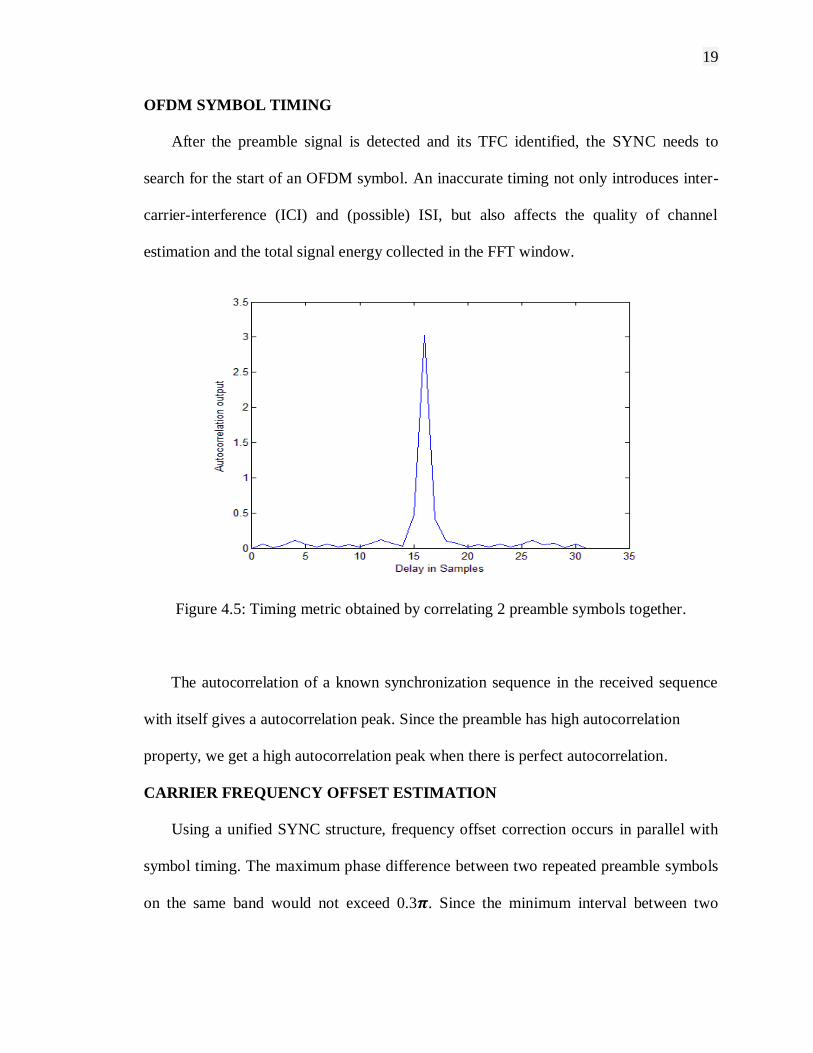
Figure 4.5: Timing metric obtained by correlating 2 preamble symbols together.

The autocorrelation of a known synchronization sequence in the received sequence

with itself gives a autocorrelation peak. Since the preamble has high autocorrelation

property, we get a high autocorrelation peak when there is perfect autocorrelation.

CARRIER FREQUENCY OFFSET ESTIMATION

Using a unified SYNC structure, frequency offset correction occurs in parallel with

symbol timing. The maximum phase difference between two repeated preamble symbols

on the same band would not exceed 0.3 . Since the minimum interval between two

20

repeated preamble symbols on the same band in all TFCs would not exceed 3 symbol

periods, we estimate the phase of the Autocorrelation value for 2 consecutive symbols

1= r k * r k+3 (4.2)

Where,

rk is the kth OFDM symbol

rk+3 is the symbol delayed by 3 symbol periods

1 is the autocorrelation output of the first symbol with another symbol delayed by

3 symbol periods

Since the phase of ȓ1 is given by p12 NSf1T, we could get the frequency offset

estimate f1 by

(4.3)

Where,

pk , 6 … is the delay between 2 consecutive symbols on the same band

p1 is 3

Ns is the number of subcarriers in each symbol

T is the symbol period

f1 is the initial frequency offset estimate

Iterative CFO estimation algorithm takes advantage of different values of pk to

estimate fine carrier frequency offset. The initial phase estimate is then used to

compensate for the phase of a autocorrelation value for 2 symbols separated by 6 symbol

periods.

21

= e – π f1 p2 Ns T (4.4)

Where,

p2 is 6

is the autocorrelation output of the symbol with a symbol delayed by 6 symbols

Though phase offset has already been compensated, we could still get fine carrier

frequency offset estimate f2 by dividing by the term p2 2 NS T

(4.5)

The new phase offset obtained is added with the initial phase estimate to get the

final phase estimate.

f2 = f1 + f2 (4.6)

Figure 4.6: Structure of an iterative Carrier Frequency Offset (CFO) estimator.

4.2.2 FFT:

Once Cyclic Prefix is removed from every symbol, it is sent to a FFT block which

converts the symbols back to frequency domain. The FFT output takes two paths – one to

create a channel estimate and the other as an input to an equalizer.

(k=0,1,….N-1) (4.7)

22

Where,

x(n) is complex time domain data sent on k/Nth

frequency

k/N, k=0,1,…,N-1 frequency term is orthogonal to every other frequency term

4.2.3 CHANNEL ESTIMATION:

Figure 4.7: Pilot subcarriers arrangement in an OFDM symbol.

Since every OFDM subchannel can be viewed as a flat fading channel, we decided to

use Least Squares Channel Estimator with pilot symbols inserted at the head of the packet

(in the frequency domain). The received pilot symbol in kth

subchannel relates to the

transmitted pilot symbol in the same subchannel by the equation:

(4.8)

In the LS estimator, the goal is set to minimize , where

denote the received pilot symbol vector and channel frequency response vector

respectively. Matrix is a matrix whose diagonal elements are composed of the

transmitted pilot symbols. is just matrix form convolution equation. By solving the

minimization problem above, we can estimate

23

4.2.4 EQUALIZER

OFDM Equalizer is significantly simplified due to the property of narrowband

subchannel. For every subchannel, we equalize the symbol by using this expression

.

4.2.5 DIVERSITY

Since every OFDM symbol is sent on 2 bands, we could make use of the both the

signals using diversity to improve the BER performance. We make use of Maximum

Ratio Combining technique where we combine all the signals because of multipath in a

co-phased and weighted manner so as to have the highest achievable SNR at the receiver

at all times.

Figure 4.8: Maximal Ratio Combiner.

Where,

r1, r2 ….rL are multipath copies of the transmitted signal

are complex gains associated with each path

is the complex conjugate of the channel estimate

(4.9)

24

The output of the combiner ѓ is then decoded to see an increase in BER performance

4.3 SIMULATION

Table 4.1: Simulation parameters.

Parameter Value

NSD : Number of data subcarriers 100

NSG : Number of null carriers 28

Number of total subcarriers used 128 (= NSD + NSG)

Subcarrier frequency spacing 3.906 MHz (= 500 MHz/128)

TFFT: IFFT/FFT period 256 ns (1/ F)

TCP: Cyclic prefix duration 64 ns (= 32/500 MHz)

TSYM: Symbol interval 320 ns (TCP + TFFT )

Modulation used in each subcarrier QPSK

Types of channel 1. AWGN channel

2. UWB channel

Diversity

1. Symbol Diversity

2. Multicarrier diversity

(Random subcarriers)

3. Multicarrier diversity

(Prior channel information)

25

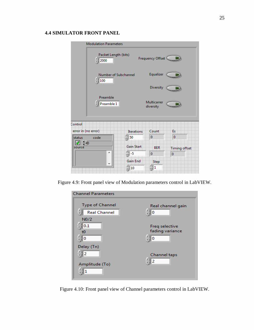
4.4 SIMULATOR FRONT PANEL

Figure 4.9: Front panel view of Modulation parameters control in LabVIEW.

Figure 4.10: Front panel view of Channel parameters control in LabVIEW.

26

4.5 Channel

There are 2 types of channels defined in this experiment and BER performance has

been evaluated for each channel by considering several critical factors.

4.5.1 AWGN Channel

According to the AWGN channel specifications, the received signal y(t) can be expressed

as an addition of the transmitted signal x(t) and white Gaussian noise w(t). If we sample

the received signal y(t) according to the relation t= nT where n=0,1,....N-1, we can

express y(n) as

y(n) = x(n) + w(n) (4.10)

where,

w(n), n=0,1..N-1 is independent and identically distributed random variable and

follows a normal distribution with mean 0 and a deviation of 0.1 [N( 0,(0.1)2 )]

y(n) is also a independent and identically distributed Gaussian random variable

[ N( x,(0.1)2 ) ]

4.5.2 UWB Channel (Frequency Selective Fading)

This channel model incorporates a strong multipath, with several overlapped replicas

of a transmitted signal. The replicas of the propagating signal are equally spaced in time,

with amplitudes that depend on both distance and delay. The model assumes that all

channel parameters are random variables with specific, well defined distributions. The

channel frequency response can be expressed as follows:

(4.11)

27

Where,

is the gain of each multipath component

is the delay in samples between any two consecutive multipath components

N is the number of multipath components

k and are constants

The shape of the channel transfer function depends on 3 critical factors:

Distance ‘D’, since channel gain ‘ n‘is inversely proportional to the distance (e-D

).

Relative Delay ‘ n / 0 ‘, since increase in delay decreases the multipath effect.

We consider some realizations of the channel frequency response based on the delay

between the multipath components ( n) keeping o and D constant.

(a) Modulus of channel transfer function (b) Modulus of channel transfer function

| H(f) |2 with n = 2 ns, 0 = 15 ns. | H(f) |2 with n = 4 ns, 0 = 15 ns.

28

(c) Modulus of channel transfer function (d) Modulus of channel transfer function

| H(f) |2 with n = 8 ns, 0 = 15 ns. | H(f) |2 with n = 16 ns, 0 = 15 ns.

(e) Modulus of channel transfer function (f) Modulus of channel transfer function

| H(f) |2 with n = 32 ns, 0 = 15 ns. | H(f) |2 with n = 64 ns, 0 = 15 ns.

Figure 4.11: Modulus of UWB channel transfer function |H(f)|2 for different scenarios.

29

As n increases, the multipath effect decreases and the channel transfer function

tends to resemble the transfer function of an ideal channel. Note that the value of affects

the position and the number of the peaks in the transfer function.

For high o, there is a high and narrow peak, while the peak widens and lowers when

o decreases. Gain varies with according to an exponential law; when o decreases, ɑn

decreases rapidly, leading to a flatter transfer function.

(a) Band 1 Channel Impulse Response – Real part. (b) Band 1 Channel Impulse Response – Imag part.

(c) Band 1 Channel Impulse Response – Real part. (d) Band 1 Channel Impulse Response – Imag part.

30

(e) Band 1 Channel Impulse Response – Real part. (f) Band 1 Channel Impulse Response – Imag part.

Figure 4.12: Channel impulse response of 3 bands for a channel scenario with n = 2 ns,

0 = 15 ns and N=10.

31

Chapter 5

Experiments and Results

5.1 EXPERIMENTAL SETUP FOR BER PERFORMANCE IN AN AWGN

CHANNEL

The goal of this experiment is to evaluate the BER performance of the system when

UWB signal is passed through an AWGN channel. Each noise component w(n) is a

complex Gaussian RV with a variance of 0.01 / 0.1 and it is added to every symbol

transmitted. A simple equalizer has been designed to cancel the channel impairments by

equalizing the output using the channel estimate. We observe that as signal power

increases, BER decreases.

Figure 5.1: BER curve showing the performance in an AWGN channel

with noise variance N0=0.01.

32

5.2 EXPERIMENTAL SETUP FOR A SYSTEM WITH / WITHOUT

DIVERSITY

The goal of this experiment is to evaluate the BER performance of the system

using symbol diversity and multicarrier diversity and compare the results to see any

improvement. We have evaluated the SNR-BER curve for six different channel

scenarios based on the values of n, 0 and N (Number of multipath components).

To evaluate the performance improvement, experiments were performed by sending

the data on more than one band and on more than one subcarrier in an OFDM

symbol.

1. No diversity scheme where we just perform equalization to remove the channel

effects such as dispersion, ISI etc.

2. Multiband Diversity scheme where we transmit an OFDM symbol on different

frequencies and make use of multiple copies of the same signal to improve the

BER performance.

3. Multicarrier Diversity scheme where we transmit the same data on different

subcarriers orthogonal to each other in an OFDM symbol and improve the BER

performance.

4. Multicarrier Diversity scheme knowing the channel information where we

improve the performance by knowing the periodicity of the channel transfer

function and sending the data on different subcarriers sensibly.

Multicarrier Diversity

When we send an OFDM symbol on a band, data is actually sent on 100 parallel

33

subcarriers with a spacing of 3.9 MHz. In multicarrier diversity, we send the same data

on two different subcarriers i.e. the same data on subcarrier 1 and subcarrier 50 and make

use of diversity to improve the BER performance. For example, we consider a channel

transfer function with n= 1 sample

Figure 5.2: Channel Frequency spectrum showing the frequencies on which same

data is sent not knowing the channel information in advance.

The diagram shows that we send the same data on subcarrier frequencies marked in

red, blue and yellow and combine their outputs at the receiver to improve the

performance. Since we have the channel estimate for each band i.e an estimate for each

subcarrier within a band, we can combine the outputs of the subcarriers with the same

data by

ȓ (5.1)

34

Where,

rk,i is the ith subcarrier of the kth OFDM symbol

is the complex conjugate of the channel estimate of the ith subcarrier

frequency in that band.

rk,i +50 is the i+50th subcarrier of the kth OFDM symbol

ȓ is the combined output of the same data sent on 2 different subcarriers.

Multicarrier diversity with prior channel information

As a special case, we can improve the performance by sending data on specific

subcarriers sensibly if we know the channel information in advance. In this case, we send

the same data on two different subcarriers – subcarrier frequency experiencing a good

fade and a subcarrier frequency experiencing less fade. We consider the same channel

transfer function with n= 1 sample.

Figure 5.3: Channel Frequency spectrum showing the frequencies on which same

data is sent knowing the channel information in advance.

35

The diagram shows that we send the same data on subcarrier frequencies marked in

red and blue and combine their outputs at the receiver to improve the performance.

When an OFDM symbol is sent on this band (2.41GHz ~ 2.46GHz), we see that the first

subcarrier frequency has less fade and the last subcarrier frequency has more fade. By

knowing this channel information, we send the same data on subcarrier 1 and subcarrier

100 sensibly to make full use of multicarrier diversity.

We evaluate the BER performance of the system by performing multiband diversity

and multicarrier diversity and see its influence in the following set of diagrams.

(a) BER curves showing the performance in a UWB channel with n = 6 ns, 0 = 15 ns,

Number of Channel taps = 1

The results show that BER improves by using diversity mechanism. Since we have a

tapped delay line channel model with equally-spaced taps ( n) and an exponential transfer

function, subcarrier frequencies in every OFDM symbol will experience similar fading

for constant o and N.

36

(b) BER curves showing the performance in a UWB channel with n = 6 ns, 0 = 15 ns, Number of Channel taps = 4

(c) BER curves showing the performance in a UWB channel with n = 6 ns, 0 = 15 ns, Number of taps = 7

37

Multicarrier diversity shows a marginal increase in performance over diversity as

the chance of sending the data on two frequencies with different fades is high. BER

performance is the best when we perform multicarrier diversity knowing the channel

information in advance. As the delay between the multipath components is increased

( n = 12 ns), the overall BER performance of the system improves for both multiband

diversity and multicarrier diversity compared to the previous scenario ( n = 6 ns)

considered.

(d) BER curves showing the performance in a UWB channel with n = 6 ns, 0 = 15 ns,

Number of Channel taps = 1

38

(e) BER curves showing the performance in a UWB channel with n = 12 ns, 0 = 15 ns,

Number of Channel taps = 4

(f) BER curves showing the performance in a UWB channel with n = 12 ns, 0 = 15 ns, Number of Channel taps = 7

Figure 5.4: BER curves showing the performance in a UWB channel using

an equalizer, symbol diversity and multicarrier diversity

39

5.3 EFFECT OF MULTIPATH COMPONENTS (N):

Experiments were performed to see the influence of multipath components on the

BER keeping n and o constant. For the same delay between any 2 consecutive multipath

copies ( n=3 samples), BER improves marginally when the number of channel taps

increases for diversity and multicarrier diversity. Increase in the number of channel taps

increases the number of multipath copies of the same signal. The more the number of

copies, better is the BER performance. In this experiment, we compare the BER results of

the system with no diversity, diversity and multicarrier diversity for different number of

multipath components (N).

(a) BER curve showing the performance in a UWB channel with n = 6 ns and 0 = 15 ns

40

(b) BER curve showing the performance in a UWB channel with n = 12 ns and 0 = 15 ns

Figure 5.5: BER curves showing the performance in a UWB channel for

different values of N

5.4 EFFECT OF n:

Experiments were performed to see the influence of delay between multipath

components on the BER keeping N and o constant. As the delay between the multipath

components n increases, the channel transfer function becomes more flat with less fade

and the BER performance improves. Increase in n decreases the multipath effect

decreases and BER also decreases for the same SNR. In this experiment, we compare the

BER performance for a system with no diversity/ diversity / multicarrier diversity for

different values of n .

41

(a) BER curve showing the performance in a UWB channel with 0 = 15 ns and N=4

(b) BER curve showing the performance in a UWB channel with 0 = 15 ns and N=7

Figure 5.6: BER curves showing the performance in a UWB channel for

different values of N

42

Chapter 6

Conclusion and Future Direction

6.1. Conclusion

The thesis explores the design and implementation of a MB-OFDM UWB system on

a LabVIEW platform and evaluates its performance by passing the UWB signal through

different channel scenarios controlled by few variables. Every OFDM symbol is

transmitted on one of those 3 bands depending on the Time Frequency Code (TFC). A

low complexity synchronization method was implemented keeping in mind the low

power requirement and affordability of UWB devices. A parallel autocorrelator structure

performs TFC identification, symbol timing and carrier frequency offset correction

together making the synchronization very simple. There was scope for improving the

performance by sending the same data on multiple bands or multiple subcarriers within

an OFDM symbol to exploit diversity at the receiver. Experiments were conducted to

study the relative increase in performance of the system using symbol diversity,

multicarrier diversity without knowing channel information and multicarrier diversity

knowing channel information in advance. The results show that symbol diversity

performance is better than a system with no diversity scheme and multicarrier diversity is

better than symbol diversity. BER performance is the best when multicarrier diversity is

performed knowing the channel information in advance.

43

6.2. Future Work

PAPR REDUCTION

OFDM signal exhibits a high Peak-to-Average Power Ratio (PAPR) and a high PAPR

necessitates the Power Amplifier to be linear within a wide dynamic range. PAPR

reduction techniques like Tone Reservation and Selective Mapping could be studied.

MULTIPLE-ACCESS SCHEMES FOR SEVERAL USERS

This system can be extended to TDMA OFDM and OFDMA system for multiple users

and its performance could be studied

DYNAMIC MODULATION TECHNIQUES

The idea of adaptive modulation is to employ high-order modulation schemes at

subcarriers with high SNR, and vice versa. With adaptive modulation, the performance of

an OFDM system can be greatly enhanced.

44

References

[1] Batra et al., Multi-band OFDM Physical layer proposal for IEEE.802.15 Task group

3a, High Rate Ultra-Wideband PHY and MAC Standard, Standard ECMA-368, Dec.

2005, ECMA, 1st Ed.

[2] R. Cardinali, L. De Nardis, P. Lombardo and M.-G. Di Benedetto,

“UWB ranging accuracy in high- and low-data-rate applications,” IEEE Transactions

on Microwave Theory and Techniques, Volume: 54, Issue: 4, Part: 2

[3] Z. Ye, C. Duan, P. Orlik, and J. Zhang, “A Low-Complexity Synchronizer

Design for MB-OFDM Ultra-Wideband Systems,” MERL Tech. Report Cambridge,

USA, Aug. 2007.

[4] H. Minn, V. Bhargava and K. Lataief, “A robust timing and frequency

synchronization for OFDM systems,” IEEE Trans. Wireless Commun., vol. 2, no. 4,

pp. 822–838, Jul. 2003.

[5] H. Liu and C. Lee, “A low-complexity synchronizer for OFDM-based UWB

system,” IEEE Trans. Circuits & Syst.-Part II, vol. 53, no. 11, pp. 1269–1273, Nov.

2006.

[6] J. G. Proakis and M. Salehi, Digital Communications, 3rd ed. New York: McGraw-

Hill, Inc., 2008

[7] T. Jacobs, Y. Li and H. Minn, “Synchronization in MB-OFDM-based

UWB systems,” in Proc. IEEE Int’l Communications Conf. (ICC ’07),Glasgow,

Scotland, Jun. 2007.

[8] http://www.eetimes.com/design/communications-design/4008964/Multiband-

OFDM-Why-it-Wins-for-UWB

45

[9] http://cegt201.bradley.edu/projects/proj2007/uwb/white_papers/MB-

OFDM_A_New_Approach_for_UWB.pdf

[10] http://www.ee.oulu.fi/~mattih/1866.pdf

[11] http://www.informi12t. com/articles/article.aspx?p=384461

[12] http://viola.usc.edu/Research/Yu-Jung%20(Ronald)%20Chang_vtc06.pdf

[13] http://www.4gamericas.org/index.cfm?fuseaction=page&pageid=1181