Impacts of U.S. Agricultural and Ethanol Policies on...

Impacts of U.S. Agricultural and Ethanol Policies on Farmland Values and Rental Rates

Jaclyn D. Kropp1 · Janet G. Peckham2 1 (Assistant Professor, Clemson University)

2(PhD Student, Clemson University)

Abstract:

Prices for prime farmland have increased significantly in recent years. But, is the dramatic

increase the result of a speculative bubble or is it consistent with market fundamentals with

increases driven by growing global demand and recent changes to U.S. agricultural and energy

policies? This research investigates the impacts of recent agricultural support policies and

ethanol policies on farmland values and rental rates. Using weighted ordinary least squares and

two stage least squares, we find that government payments, urban pressure and the proximity of

the farm to an ethanol facility have a positive impact on both farmland values and rental rates.

Keywords: capitalization; decoupled payments; ethanol; farmland values; rental rates; subsidies JEL: Q18; Q15; Q16 Selected Paper prepared for presentation at the Agricultural & Applied Economics Association’s 2012 AAEA Annual Meeting, Seattle, Washington, August 12-14, 2012 Copyright 2012 by Jaclyn D. Kropp and Janet G. Peckham. All rights reserved. Readers may make verbatim copies of this document for non-commercial purposes by any means, provided that this copyright notice appears on all such copies.

1

Impacts of U.S. Agricultural and Ethanol Policies on Farmland Values and Rental Rates

In the third quarter of 2011, land prices for prime farmland increased 25 percent relative to the

same quarter of 2010, marking the largest increase since 1977 (Oppedhal 2011). Memories of

the 1980s farm financial crisis and the recent subprime mortgage crisis have some economists

concerned that the dramatic increase in farmland values is the result of a speculative bubble.

Other economists argue that the rise in farmland values is consistent with market fundamentals

and is driven by increased demand and recent changes in U.S. agricultural and energy policies.

While there is considerable research investigating the impacts of agricultural support policies on

farmland values and rental rates (e.g., Lence and Mishra 2003; Kirwan 2009; Goodwin, Mishra,

and Ortalo-Magne 2011), very little research has addressed the specific effects of ethanol

policies. Thus, this research investigates the impacts of both agricultural support policies and

recent ethanol policies on farmland prices and rental rates.

The extent to which U.S. agricultural policies impact farmland values and rental rates is

currently debate in the farm policy literature. Kirwan (2009) investigates the impact of

agricultural subsidies on rental rates and concludes that approximately 25 percent of these

subsidies are captured by landowners in the form of higher rental payments. On the other hand, a

recent study by Goodwin, Mishra, Ortalo-Magné (2011) suggests that agricultural payments are

almost completely capitalized into farmland values and that landowners capture substantial

benefits from agricultural payments even when the policy mandates that the operator is the

payment recipient. However, both studies ignore the impacts of ethanol policies on farmland

values, land use and rental rates.

Recent U.S. ethanol policies promoting the production of corn have the potential to impact

land prices in two ways. The first impact is geographically dispersed but small in magnitude.

Policies that promote corn based ethanol increase the demand for corn, driving up the price of

corn and hence farmers plant more acres of corn. As other commodities compete with corn for

land, farmland prices increase. The second impact is larger in magnitude but more

geographically concentrated. Corn ethanol facilities increase the demand for corn locally and

decrease the cost of transporting corn to a more distance market. Thus, land near an ethanol

facility becomes more valuable and can command a higher price. While there has been some

research looking at the influence of the proximity of corn ethanol facilities on land prices

2

(Henderson and Gloy 2008), the effects of ethanol policies on land use and prices have not yet

been fully explored and quantified on a large scale.

In this paper, we use a capitalization model to examine the effects of agricultural support

policies and ethanol facility location on farmland values while controlling for other factors. The

capitalization model states that the current value of an acre of land should equal the sum of the

discounted future returns (both market returns and government payments) to that acre of land.

Although capitalization models dominate the farm policy literature, capitalization models are

based on the assumption that payments are known with certainty and received in perpetuity;

hence, these models are not well equipped to handle changing expectations or changing policy

regimes. Therefore, we also examine rental rates, which have the ability to adjust more quickly

to the changing policy environment. Specifically, we analyze the impact of market returns,

government payments, ethanol plant location, amenities and urban influences on farmland values

and rental rates. Using farm-level data from the United States Department of Agriculture

(USDA) and regression analyses (weighted ordinary least squares and two stage least squares

similar to those employed by Goodwin, Mishra, Ortalo-Magné (2011)), we find that government

payments, urban pressure and the proximity of the farm to an ethanol location have a positive

impact on both farmland values and rental rates.

The remainder of this paper is organized as follows. The next section provides an

overview of recent government policies that may affect farmland values. Specifically, the 1996,

2002, and 2008 Farm Bills are discussed as they pertain to corn. An overview of U.S. ethanol

policies is also provided. In addition, the relevant literature is discussed. The third section

reviews the capitalization model. The fourth section presents an empirical analysis of factors

affecting farmland values and rental rates. The final section discusses offers some concluding

remarks.

Overview of Agricultural Policies and Relevant Literature

Although the extent to which agriculture policies are capitalized into land values and rental rates

is currently debated in the policy literature, agricultural policies are clearly important factors to

consider when modeling farmland prices. This section provides an overview of recent

government policies that may affect farmland values. Since we are primarily interested in the

impact of recent ethanol policies promoting corn-based ethanol, we focus the discussion on

agricultural policies that support corn and ethanol producers.

3

U.S. Agricultural Support Policies

Prior to the 1996 Farm Bill (P.L. 104-127), agricultural payments were “coupled” or linked to

current production with farmers receiving payments based on their current production levels and

market prices. To comply with World Trade Organization (WTO) obligations requiring a

reduction in trade distorting domestic support, the 1996 Farm Bill was written with the goal of

heavily reducing agricultural support programs by 2002. The bill also attempted to remove the

link between payment programs and market prices for agricultural commodities. Production

flexibility contract (PFC) payments were introduced in the 1996 Farm Bill (Federal Agriculture

Improvement Reform Act) in an effort to “decouple” payments from market prices and current

production. PFC payments were paid to farm operators based on historic (base) acreage and

yields to operators with historic production (acreages and yields) of wheat, feed grains (corn,

barley, sorghum and oats), cotton, and rice (commonly referred to as program crops).

The 1996 Farm Bill stipulated the annual PFC payment rate for each crop. The annual

payment rates declined over time with PFC payments scheduled to be phased out prior to the

2002 Farm Bill. Thus, farm operators received seven years of fixed, but declining, annual PFC

payments. The total payment received by a recipient was equal to the payment rate multiplied by

the farm’s eligible payment acreage and the program yield established for the particular farm

(USDA 1996). Since the payments were supposed to be temporary, they should not be

capitalized into land values and should have only a small impact on farmland values.

Marketing assistance loans (MAL) were another form of agricultural support under the

1996 Farm Bill. MAL were designed to assist farmers by providing short-term financing, which

enabled farmers to pay their bills soon after harvest but spread their sales over the marketing

year. Non-recourse marketing assistance loans allowed recipients to forfeit the commodity

pledged as collateral to the Commodity Credit Corporation (CCC) in satisfaction of loan

repayment at maturity. Alternatively, in lieu of receiving MAL, eligible producers could receive

loan deficiency payments (LDP). LDP paid producers the difference between the market price

and the support price (loan rate). LDP were intended to minimize delivery of loan collateral to

the CCC thus reducing the costs associated with the MAL program. MAL and LDP are typically

classified as coupled payments because they are linked both to current production and current

market prices.

Furthermore, the 1996 Farm Bill contained provisions for land diversion programs that

4

removed environmentally fragile acreage from production. An example is the conservation

reserve program (CRP), which was continued from the 1990 Farm Bill. Under the program,

farmers enter sensitive wetlands or fragile farmland into the program for conservation usage for

10 to 15 years, and in return the producer receives an annual rental payment on the diverted

acreage. The program aims to reduce erosion and enhance water quality on agricultural land. The

programs also support agricultural commodity prices by reducing the supply of various

commodities. In addition, the program provides cost-share assistance for the establishment of

approved conservation practices.

In 1999, the ad hoc market loss assistance (MLA) program was introduced. MLA

payments are triggered by market prices below target prices with recipients receiving the

difference between the target price and the market price. Ad hoc disaster payments have also

been a mainstay of U.S. agricultural policy. Disaster payments are frequently implemented

following natural catastrophes such as droughts and floods. Because these payments provide

benefits that offset adverse market conditions or poor production decisions, they have the

potential to alter production decisions and ultimately impact farmland values and rental rates.

Although the PFC and MLA programs were supposed to be temporary, version of both

programs were continued in the 2002 Farm Bill (P.L. 107-17). The PFC payment program was

replaced with the fixed direct payment program and MLA program was replaced with counter-

cyclical payment (CCP) program. Fixed direct payments (FDP), like production flexibility

contract payments, were available to eligible producers of wheat, corn, barley, grain sorghum,

oats, upland cotton, and rice. Additionally new payments were established for soybeans, other

oilseeds, and peanuts. FDP were based on historic yields and acreage with payment rates

specified in the 2002 Farm Bill for all covered crops. CCP were paid to covered commodities

when the effective price was less than the target price. The effective price was the higher of the

national average market price and the national loan rate for that commodity. The target price for

corn was $2.60 per bushel for the 2002-2003 crop years and $2.63 per bushel for the 2004-2007

crop years (USDA 2002). Counter-cyclical payments were paid to historical production.

Therefore, CCP are frequently classified as partially decoupled since they are tied to current

market prices but not current production levels. Unlike PFC and FDP, CCP were not known in

advance because they were based on current market prices.

In the 2002 Farm Bill, farmers were given the option to update their base acreage and

5

yields to the past four years average acreage planted and harvested, or they could continue to use

the base acreage and yields upon which payments were calculated in the 1996 Farm Bill (1991-

1995 crop years). Therefore, not only did the government continue the decoupled support

payments it claimed to be eliminating, it allowed farmers the opportunity to increase their

payments by increasing their base acreage and yields. This set a precedent that subsequent farm

bills would allow updating of base acreage and base yields. Although both FDP and CCP were

continued in the 2008 Farm Bill, updating was not explicitly allowed. Numerous studies have

shown that updating and expectations of potential updating cause producers to alter production

decisions in the current period thus calling into question the classification of these payments as

decoupled (Goodwin and Mishra 2006; Bhaskar and Beghin 2010; Peckham and Kropp

forthcoming).

MAL and LDP were also continued in the 2002 Farm Bill with minimal changes but

these supports were extended to cover additional commodities (USDA 2002). Furthermore,

producers no longer had to enter into annual contracts for direct payments to be eligible for MAL

as in the 1996 Farm Bill. The CRP program was also continued.

The 2008 Farm Bill (P.L. 110-246) generally continued the 2002 structure of FDP, CCP,

CRP and MAL programs. It, however, changed some program eligibility criteria and payment

limitations. The bill also adjusted the target prices for CCP and the loan rates for some

commodities. However, the target price for corn was not affected. Although updating was

anticipated by some producers, updating was not allowed. However, farmers were allowed to

adjust yields and acreage to account for newly covered commodities. In addition, the bill

introduced the Average Crop Revenue Election (ACRE) program.

The ACRE program, which began in the 2009 crop year, was a new whole farm revenue

based program. Producers who enrolled in ACRE must remain enrolled until 2012. To receive an

ACRE payment, two triggers must be met. First, the actual state revenue for the supported crop

during the crop year must be less than the state-level revenue guarantee amount. Second, an

individual farm’s actual revenue for the supported crop during the crop year must be less than the

farm’s benchmark revenue. Benchmark yields at the state and farm-levels are Olympic averages

of the most recent five years. Price guarantees are averages of the marketing year price (or the

marketing loan rate reduced by 30%, if greater) for the most recent two years. If both triggers are

met, the individual farm receives an ACRE payment that is based on the state-level difference

6

between actual revenue and the ACRE guarantee per acre multiplied by a percentage (83.3% or

85% depending on the crop year) of the farm’s planted acreage, which is pro-rated based on the

individual farm’s yield history compared to the state’s yield history (Renée 2008).

Under the 2008 Farm Bill, farmers choose between the traditional CCP and the new

ACRE programs. If a farmer chooses the ACRE program he continues to receive FDP at eighty

percent of the original rate. The farmer also continues to receive MAL but at a thirty percent

reduction in the loan rate (Renée 2008). A farmer that participates in the ACRE program is no

longer eligible to receive CCP.

Agricultural support programs are designed to benefit producers by 1) increasing

agricultural returns and/or 2) decreasing the volatility of returns. Thus, different programs are

likely to have different impacts on farmland values and rental rents depending on how the

specific program benefits producers and the permanency of the program. This will be discussed

more formally in the next section.

U.S. Ethanol Policies

The US has a long history of promoting domestic ethanol production through producer

incentives, trade barriers, sustainability standards and tax credits. The Energy Tax Act of 1978

introduced ethanol subsidies that launched the U.S. ethanol industry. When first introduced, the

subsidy was in the form of a partial excise-tax exemption for the blended fuel; more recently, the

subsidy functioned as a tax credit for the blender. Although policies promoting ethanol

production are not new, policies enacted following the Energy Policy Act of 2005 (P.L. 109-

58) and the Energy Independence and Security Act of 2007 (P.L. 110-140) have led to a surge in

ethanol production since 2005.

The Energy Policy Act of 2005 and the Energy Independence and Security Act of 2007

established renewable fuel standards. These standards established sustainability thresholds with

targets for reducing carbon dioxide emissions. Biofuel blend and consumption mandates were

also established. Blend mandates require each gallon of gasoline to be blended with a

predetermined amount of ethanol, while consumption mandates set requirements that a certain

number of gallons of renewable fuel be produced and used by a given deadline. Mandates

increase the demand for ethanol. More specifically, the Energy Independence and Security Act

of 2007 required 36 billion gallons of renewable fuel usage per year by 2022, roughly four times

the amount of ethanol produced in 2007 (Tyner 2008). Of the 36 billion gallons, the act

7

mandated that 20 billion gallons must come from “advanced biofuels,” which use non-corn

feedstock sources such as switch grass or municipal waste (Tyner 2008). Since advanced

biofuels are still in their infancy, it is expected that the remaining 16 billion gallons will come

from corn-based ethanol.

The policy changes since 2005 created a surge in demand for corn to be used in ethanol

production. As a result, demand for corn increased and corn prices rose quickly. Other

commodities that compete with corn for acreage or use corn as an input also experienced price

increases. As commodity prices rose and these prices were expected to remain high, the higher

commodity prices became capitalized into agricultural land prices accounting for higher

farmland price across the US.

Furthermore, ethanol production has another affect on farmland values that is larger in

magnitude but smaller in scope geographically. An ethanol plant can have a strengthening effect

on the local basis. The basis is the difference between the cash market price and the futures

market price. The basis normally reflects transportation costs of transporting the commodity to

market. When the cash price is under the futures price and the basis is said to be “weak.”

Strengthening the basis refers to an increase in cash market prices without a corresponding

change in the futures market price. An ethanol facility causes the cash price to increase in the

local market by increasing the demand for corn. In addition, producers experience higher returns

due to lower transportation costs. As increased returns are capitalized in land values, farmland in

close proximity to the ethanol plant becomes more valuable.

McNew and Griffith (2005) examine how the construction of an ethanol plant affects the

local basis. They find, on average, the basis increases 5.9 cents per bushel of corn over a 150

square mile area around the plant. The change in basis varies largely over distance. The basis

increases were largest closest to the plant location, and diminishing basis increases were

observed as the distance from the plant increased. The changes in basis, like government

policies, can be viewed as permanent or transitory, which affects how basis changes are

capitalized into farmland values.

Recent Relevant Land Pricing Studies

Numerous previous studies have investigated the determinants of farmland prices. To date, three

major land pricing models have emerged in the agricultural policy literature. These models

included supply and demand, capitalization, and hedonic pricing models. However, due to

8

simplicity of estimation and calculation, capitalization models dominate the agricultural policy

literature. The capitalization model assumes that the price of an acre of land is the sum of the

discounted future returns associated with the acre of land over a specific time period. The model

generally assumes that land is an infinitely lived asset. Some studies have shown the validity of

capitalization models using cointegration (Campbell and Shiller 1987; Clark, Klein, and

Thompson 1993). Cointegration models are used to define the difference between two time series

that move together such as the prices of agricultural commodities and agricultural land prices. If

the capitalization model, also known as the present value model, is correct, a linear combination

of the variables, which is called the spread, is stationary.

Given the large number of previous studies, we focus our discussion on the research most

relevant to our analyses. These previous studies highlight the importance of market returns,

government payments, urban influences, natural amenities, and ethanol plant locations in

determining land values.

Following earlier work, Goodwin, Mishra, and Ortalo-Magné (2003) combine multiple

product returns into one market return in their analysis of farmland values using farm-level

USDA data from 1998-2001. They also include government payments and urban pressure in

their land price models. Urban pressure is a major factor influencing agricultural land values that

has become more significant recently. As urban pressures close in on agricultural lands, the

opportunity cost of maintaining the farmland in agricultural use increases.

Goodwin, Mishra, and Ortalo-Magné (2003) find a dollar increase in government

support payments leads to a $4.69 per acre increase in farmland values. The authors also analyze

the impacts of the various types of government payments by disaggregating government

payments into loan deficiency, disaster, Agricultural Market Transition Act (MLA and PFC), and

CRP payments. Their results suggest that the source of the payment influences the magnitude of

the effect. Loan deficiency payments have the largest effect on land prices with an additional

dollar of payment raising farmland values $6.55 an acre. An additional dollar of disaster relief

payments increase agricultural land values by $4.69 an acre. One additional dollar of

Agricultural Market Transaction Act money, which was set to end in 2002 with the FAIR act,

raises per acre land values $4.94. This value seems high if farmers truly believed that the benefits

would end in 2002. It appears that the agricultural community correctly predicted that the 2002

Farm Bill would continue these payments. The authors find that conservation reserve payments,

9

which involve land removal from production, are negatively correlated with land values.

However, these values should be taken cautiously because the magnitude of effect changes from

year to year and across regions.

While numerous academic studies have analyzed the effects of agricultural support

policies on farmland values, considerably fewer studies focus on the effects of these policies on

rental rates. Since 45.3 percent of agricultural land is operated by someone other than the owner

(USDA 1999), understanding the impact of agricultural support policies on rental rates is

important. Three notable expectations are recent studies by Kirwan (2009), Patton et al. (2008),

and Goodwin, Mishra, and Ortalo-Magné (2011). Kirwan, using panel farm-level data taken

from the Agricultural Census for the years 1992 and 1997 and an instrumental variables

approach, finds 20 to 25 percent of agricultural support payments are capitalized into land rental

values (Kirwan 2009). Patton et al. (2008) and Goodwin, Mishra, and Ortalo-Magné (2011)

disaggregate agricultural support payments into decoupled and coupled payments and employ an

instrumental variables approach to account for payment uncertainty at the time rental agreement

terms are negotiate. Their results indicate different types of agricultural payments have different

effects on rental rates. Goodwin, Mishra, and Ortalo-Magné (2011) find that landowners extract

a large portion of agricultural support program benefits through higher rental rates. We use an

instrumental variables approach similar to Goodwin, Mishra, and Ortalo-Magné (2011), while

also accounting for the effects of recent ethanol policies.

Henderson and Gloy (2008) examine the impact of ethanol plant location on farmland

prices using farmland values estimated by local agricultural bankers. Their empirical results

show that agricultural amenities, government payments and urbanization characteristics exhibit a

positive relationship with farmland values. The results also indicate that the distance from an

ethanol plant is negatively related to farmland values. Therefore, farmland values are higher

closer to operating ethanol plants. For every mile increase in distance from an ethanol plant, land

prices decrease $1.44 per-acre for the 2006 data. Using the 2007 data, this figure rises to $2.14

per-acre, indicating the affects are increasing as the basis change is viewed as more permanent.

One shortcoming of Henderson and Gloy’s (2008) article is that the farmland value data

are gathered from an opinion survey of bankers financing agricultural land sales. The authors

argue that these bankers should have a good idea of farmland values in their region. We build

upon Henderson and Gloy’s (2008) work by using a larger dataset of individual farm-level data

10

collected annually by the USDA in the Agricultural Resource Management Survey (ARMS). We

examine both farmland values and rental rates.

Policy Effects on Farmland Values and Rental Rates

Following Goodwin, Mishra, and Ortalo-Magné (2011), we allow the value of a parcel of land to

be the present discounted value of expected cash flows from agricultural activities plus the value

of the option to convert the land to non-agricultural use.

�� ∞

�� ! "#� ��$��

where ��is the value of the parcel of land, � is the expectation operator, �� is the sum of

market returns at time t, �� is the sum of government payments at time t, �� is equal to the

opportunity cost of keeping the land in agricultural use, which is a function of urban pressures

and natural amenities on the parcel of land and neighboring parcels, and � is the discount rate.

The discount rate reflects the riskiness of the stream of cash flows.

Like returns, urban pressure positively affects agricultural land prices. Urban pressure

raises the opportunity cost of keeping the parcel of land in agricultural use. While urban pressure

increases the likelihood that the land will be converted to non-agricultural uses, natural amenities

decrease the likelihood that the land will be converted to non-agricultural uses. However, both

factors increase the value of the parcel.

Market returns can further be divided into commodity specific returns, while government

payments can be disaggregated into the various types of payments discussed in the previous

section. The various sources of returns are likely to have different discount rates because each

type of return has a different level of risk and a different degree of permanency.

In an attempt to analyze the impacts of each payment type on farmland values, we

disaggregate government payments into four types of payments in the empirical analysis: 1)

decoupled payments (PFC payments, FDP and CCP), 2) CRP payments, 3) LDP and 4) disaster

payments (MLA). Total government payments are thus defined as �� %�� &'� � �('� � )&'� � &�*�*��

where �� represents government payments, &'� represents decoupled payments, �('� represents CRP payments, )&'� represents LDP, and &�*�*�� represents disaster payments.

In general, government payments increase agricultural returns and reduce agricultural

income volatility. Hence, government payments are likely to have a positive impact on land

11

prices. However, as previously discussed some payments are tied to historical averages such as

decoupled payments, while others are triggered by current market conditions such as LDP and

disaster payment, thus the discount rate for each type of government payment should reflect the

certainty and permanency of the payment. Let �+,- be the discount rate associated with

aggregate payments and �./, �01/, �2./, and �.34 be the discount rates associated with DP, CRP,

LDP and Disaster respectively:

�� 5� �� +,-�� &'�� ./��

�('�� 01/�� )&'�� 2./��

&�*�*�� .34�� Substituting �� 5� into �� yields,

�� 6�� 78 9:;<=�>��?3@ABCD>�> � ./>��?3EF�> � 01/>��?3GHF�> � 2./>��?3IEF�> � .34:4�=;>��?3EJK�>∞�� L � �� ! "#� ��$��. where �9:;<=� is the discount rate associated with market returns. Note, � is not the sum of the

individual discount rates because of the non-zero covariance across the various types of

government payments and market returns (i.e., disaster payments are received when market

returns are low).

Another factor that impacts farmland values, especially in the Midwest, is the location of

ethanol facilities. Corn ethanol facilities increase the market returns �� associated with

corn production on land in close proximity to the facility by increasing the demand for corn and

lowering transportation costs. Thus, parcels of land in close proximity to ethanol plants should be

more valuable.

The capitalization model assumes returns are known with certainty. However, this is

generally not the case, especially when faced with changing policy environments. On the other

hand, rental rates reflect the price of land input used in the agricultural production process and

rental rates do not face many of the same problems as land values since they are adjusted every

few years. Yet, rental rates tend to be effected by the same factors that influence land prices and

perhaps provide a better measure of the opportunity costs of the land moving away from

agriculture. For these reasons, both land value per acre and rental rates per-acre are analyzed in

this paper.

When the price of a commodity increases, this increases the demand for the inputs used

to produce the commodity. More formally, a corn producer solves the profit maximization

problem:

12

�� M� 11

( ,..., )m

m j jj

Max pf x x r xπ=

= −∑

where N�O�! P OQ� is the production function for corn, which is a function of m inputs

(O�! P ! OQ� , p is the unit price of the corn output and ( �! P ! Q� are the prices of inputs.

Without loss of generality, the j first order conditions that solve Eq. 5 are:

�� R� STSUV � W SXYUVZSUV [ \ � ].

Eq. 6 indicates that when policies that increase the price of corn are enacted (e.g. ethanol

policies), the rental rate for a parcel of land used to produce corn must also increase (assuming

the marginal productivity of land, SXYUVZSUV ! has not changed).

Empirical Analysis

In this section, we analyze the determinants of farmland values and rental rates.

Measurement Error and Endogeneity:

The capitalization model presented in the previous section states that the value of a parcel of land

is the discounted value of expected cash flows from agricultural activities plus the value of the

option to convert the land to non-agricultural use. Additionally, rental rate are also determined

based on expected returns. However, data available for the analyses consist of the realized values

of the cash flows rather than the expected values. As a result, researchers face classic errors-in-

variables problems due to measurement error in the variables, which can lead to insignificant and

inconsistent estimators (see Goodwin, Mishra, and Ortalo-Magné (2011) for a thorough

discussion). In addition, there is an endogenous relationship between farmland values and

government payments. To illustrate the endogenous relationship consider the fixed direct

payment program: under the FDP program more productive farmland (i.e. farmland with higher

yields) receives higher FDP payments. Thus, more valuable farmland tends to receive more

government payments. Furthermore, the location of an ethanol facility is also not exogenous.

Ethanol facilities tend to be located in areas where land is most suitable for efficient corn

production.

The standard approach to overcoming both measurement error and endogeneity is to

employ instrumental variables techniques. This requires finding instruments that are correlated

with the variable of interest but uncorrelated with the error term. Thus, in addition to weighted

ordinary least squares, an instrumental variable approach, similar to the approached used by

13

Goodwin, Mishra, and Ortalo-Magné (2011) is employed. We use five-year smoothed county

averages as the instruments. Using smoothed county averages allows us preserve more

observations. We conduct all analyses using aggregate government payments and then repeat the

analyses using disaggregated government payments. When disaggregated government payments

are used, following Goodwin, Mishra, and Ortalo-Magné (2011), LDP county averages are two-

year smooth county average. The results are similar when the five-year smooth county average

for LDP is used.

Data

We use the 1998-2008 USDA Agricultural Resource Managerial Survey (ARMS) dataset, which

consists of cross-sectional farm-level data collected annually by the USDA’s National

Agricultural Statistics Service. The dataset includes information such as the estimated market

value of land and buildings, acreage, commodity mix, value of production, output quantities,

input expenses, governmental payments by program, and farm and farmer characteristics.

Similar to Goodwin, Mishra, and Ortalo-Magné (2011), expectations of government payments

are measured by a proxy variable constructed from historic average county-level government

payments using USDA Farm Service Agency (FSA) data. FSA data is unpublished and was

obtained through a Freedom of Information Act (FOIA) request. The data consist of annual

government payment information by recipient for each program type and annual county-level

acreage reports by commodity. Additionally, using ethanol plant location data obtained from the

Renewable Fuels Association (2010) and the American Coalition for Ethanol (2010), we

constructed a dataset of all corn-based ethanol facilities. The dataset includes information

pertaining to the date of first operation and capacity. The operational date of each ethanol facility

was obtained through the facilities website, news articles about the facility, or by calling the

facility. All monetary values used in our analyses are deflated by the consumer price index (CPI)

to obtain 2008 equivalent real values. Unless otherwise stated, all variables are computed on a

per-acre basis. We limit the analysis to farms with more than 50 acres operated.

Since we are primarily interested in the impacts of corn ethanol policies, the analysis is

limited to the USDA geographic region defined as the heartland, where the majority of the eight

million acres of corn planted in the US annually is grown. Currently, this region also has 128

ethanol facilities using corn as a feedstock. Three states are fully included in the heartland

14

region: Indiana, Illinois, and Iowa. Six other states are partially included in the heartland region:

1) Ohio, 2) Kentucky, 3) Missouri, 4) Nebraska, 5) South Dakota and 6) Minnesota.

Dependent variables

The first dependent variable analyzed is the real per-acre value of land (LAND). ARMS

respondents are asked to estimate the total value of land and buildings. Respondents are also

asked to report the total value of buildings. Using these two responses, land value is constructed

as the difference between the value of land and buildings and the value of buildings. Negative

values resulting from this calculation are most likely due to confusion about the questions or

poor estimation on the part of the respondent. Hence, negative land values are eliminated from

the analysis. To obtain land value on a per acre basis, land value is divided by total acres owned

(ACRESOWN). While our measure of farmland value relies on producers’ estimates, we assume

that farmland owners tend to track local land sales and thus should be able to provide a valid

assessment of the value of their land. Following Goodwin, Mishra, and Ortalo-Magné (2011), we

eliminate outliers by dropping observations with LAND values less than $200 or greater than

$20,000. The truncation removes outliers due to poor estimation or confusion on the part of

respondents, non-typical agricultural properties such as vineyards, and properties with non-

typical parcel characteristics such as river frontage (Goodwin, Mishra, and Ortalo-Magné 2011).

The land value truncation removed only two percent of the observations. As shown in table 1, the

average value for LAND in the restricted sample is $2,228.44 per-acre.

The second dependent variable is real cash rental expense per-acre (RENT). The real

rental rate per-acre (RENT) is obtained by dividing the total dollar amount paid for cash rent by

total the number of acres rented on a cash basis. To remove outliers, observations where RENT is

less than $0 or greater than $2,000 are dropped from the analysis. As shown in table 1, the

average value for RENT in the heartland region after truncation is $81.73 per acre.

Independent Variables

Table 1 contains two sets of summary statistics for the independent variables. The first set of

summary statistics corresponds to the sample for the farmland value (LAND) analyses, while the

second set corresponds to the sample for the rental rate (RENT) analyses.

Table 1 also presents summary statistics for five variables which are not regressors:

ARCES, CORN, ARCESOWN, TENURE and FARM ACRES. ARCES represents the total number

of acres operated by the farm operator. CORN is the number of acres of corn harvested by the

15

farm. On average, farms in the rental rate sample operate more acres and harvest more acres of

corn than farms in the farmland value sample. ACRESOWN is the number of acres owned by the

farm operator. TENURE is the ratio of acres owned to acres operated. TENURE is lower for

farms in the rental rate sample, suggesting these farms rent a higher proportion of operated acres.

FARM ACRES is the total farmland acres in the county calculate from FSA data. This value is

used to compute county-level historic averages on a per-acre basis.

As suggested by the capitalization model, market returns are included as independent

variables in all regression models. Market returns are disaggregated into real livestock sales

(LIVESTOCK) and real crop sales (CROP) per-acre operated. All variables are constructed on a

per-acre operated (ACRES) basis unless otherwise specified.

Farm-level government payments are also reported on ARMS. We conduct the analyses

using real aggregate government payments per-acre (�� and then repeat the analyses by

disaggregating government payments into decoupled payments (DP), conservation payments

(CRP), loan deficiency payments (LDP), disaster payments (DISASTER) and other government

payments (OTHER) to examine the impact that each type of payment has on farmland values and

rental rates. DP include PFC payments, FDP, and CCP in years where they exist. CRP consists

of wetland conservation payments and conservation reserve program payments. LDP and

DISASTER are as previously defined. OTHER represents all other government payments. On

average, farms in the farmland value sample received $23.39 of real government payments per-

acre, while farms in the rental rate sample received $26.27 of real government payments per-

acre.

Urban influence is measured through the 1993 Rural-Urban Continuum Code (URBAN),

commonly referred to as the 1993 Beale Code. The Rural-Urban Continuum Code is a county

level classification (0-9) determined by the county population and if the county is a metropolitan

area, adjacent to a metropolitan area, or not. An URBAN score of 0 indicates the county is a

metropolitan area with an urban population greater than 1 million. An urban population means a

population that lives in cities or suburbs. An URBAN score of 1 indicates the county is a fringe

county close to a metropolitan area with an urban population greater than 1 million. A score of 2

indicate the county is a metropolitan area with an urban population between 250,000 and 1

million. A score of 3 indicates the county is a metropolitan area with an urban population less

than 250,000. Non-metropolitan area scores range from 4-9. A score of 4 indicates the county is

16

adjacent to a metropolitan area with an urban population of 20,000 or more. A score of 5

indicates the county is not adjacent to a metropolitan area with an urban population of 20,000 or

more. A score of 6 indicates the county is adjacent to a metropolitan area with an urban

population of between 2,500 and 19,999. A score of 7 means the county is not adjacent to a

metropolitan area with an urban population of between 2,500 and 19,999. A score of 8 indicates

the county is adjacent to a metropolitan area with an urban population of less than 2,500. A score

of 9 means the county is not adjacent to a metropolitan area with an urban population of less than

2,500. Beale Code classifications are contained in the ARMS dataset.

County-level population growth and population per farmland acre are included as

additional measures of urban pressure. County-level population estimates are intercensal

estimates obtained from the U.S. Census Bureau (2011). County-level population growth rates

(POPGROWTHt) are calculated as the change in county population divided by the county

population at the beginning of the period. Population per farmland acre (POPULATIONt) is

calculated by dividing the county-level population estimate by the total farmland acres (FARM

ACREt) in the county. Farmland acres were obtained from unpublished USDA FSA data.

Like urban pressure, natural amenities should have a positive effect on farmland values.

County-level natural amenities (AMENITY) are measured by a z score constructed by the USDA

(2004). The z score accounts for average temperatures, topography, and surface water.

Another factor influencing agricultural land values is the proximity of the parcel to an

operating local ethanol plant. Following the implementation of policies promoting corn-based

ethanol, numerous additional ethanol plants began operating in the heartland region. As

previously discussed, a local operating ethanol plant can reduce transportation costs and increase

agricultural returns for nearby farms. Ideally, we would include the distance of the parcel to the

closest corn-based ethanol facility as an independent variable. While we have the exact location

of ethanol facilities, we do not know the exact location of each ARMS respondent and hence

cannot construct this variable. To protect the confidentiality of the respondent, researchers are

only allowed to view ARMS respondents’ zip codes. Thus, we create a series of variables used to

proxy for the distance to the closest ethanol facility.

Using the zip code of the ethanol facility, an indicator variable (ETHANOLCOUNTYt)

was created that assumed a value of 1 if there is an operating ethanol facility in the same county

17

as the farm at time t and zero otherwise.1 Unfortunately, zip codes and counties do not form a

one to one matching; a zip code can be partially contained in multiple counties. Thus, when

creating ETHANOLCOUNTYt, the county that contains the largest area of the zip code was the

county deemed to contain the ethanol facility. However, because zip codes can span more than

one county, it is possible that the ethanol facility is actually located in a different county and

ETHANOLCOUNTYt is incorrect. Less than 10 percent of the counties in the sample had an

operating ethanol facility. An additional variable, NUMCOUNTYt, was created that represents

the number of ethanol facilities in the county at time t; some counties have more than one

ethanol facility and multiple ethanol facilities are likely to further increase farmland values. We

recognize that an ethanol plant within the county may not be the best proxy since there could be

a plant closer in an adjacent county.

Also, the impact of an ethanol facility on farmland values is likely to extend beyond the

county in which the facility is located. McNew and Griffith (2005) find, on average, the basis

increases 5.9 cents per bushel over a 150 square mile area around the plant. Hence, an indicator

variable, ETHANOLMULTt, was created that takes a value of 1 if there is an ethanol facility in

the county or neighboring county. NUMMULTt represents the number of ethanol facilities in the

county or neighboring county.

Weighted Ordinary Least Squares Regression Results

Using weighted ordinary least squares (OLS), we conduct separate analyses using farm-level

actual realized aggregate government payments, farm-level actual realized disaggregated

government payments, historic county-level smoothed average aggregate government payments,

and historic county-level smoothed average disaggregated government payments. For each of

these analyses, we conduct separate analyses for ETHANOLCOUNTYt, ETHANOLMULTt,

NUMCOUNTYt and NUMMULTt. The analyses are conducted for both dependent variables. The

results are summarized in tables 2-13.

All monetary values contained in the dataset are in $100/acre. Thus, in all regression

analyses, coefficient estimates associated with non-monetary variables must be adjusted by

1 We also conducted the analyses using an indicator variable that assumed a value of 1 if there is an operating ethanol facility in the same zip code as the as the farm at time t and zero otherwise. The results are similar but larger in magnitude. This confirms that the effect of the ethanol plant is largest closest to the ethanol facility location. These results are available from the authors upon request.

18

multiplying by 100 to determine the impact on farmland values or rental rates per-acre. For

example, if the coefficient on ETHANOLCOUNTYt is 7.4058 (model 1), then, on average, the

value of an acre of farmland in a county with an ethanol facility is $740.58 higher than an acre of

similar farmland in a county without an ethanol facility. No adjustment is needed to interpret the

coefficients on monetary values such as CROP or GOV. Furthermore, if we assume that the

discount rate is constant and the various returns (from market sales and government payments)

are expected to grow at a constant rate, then the inverse of the regression coefficients on returns

in the models of farmland values are capitalization rates. The regression coefficients on returns

in the models of rental rates can simply be interpreted as the proportion of the return passed on to

the landlord in the form of higher rental payments.

URBAN is included in all regression analyses as a categorical variable. In all models, the

coefficients are significant, indicating that urban influence has a positive impact on farmland

values and rental rates. Coefficient estimates for URBAN are not reported in the tables to due to

space constraints.

Table 2 presents the results for the determinants of farmland values when aggregate farm-

level actual realized returns are used as regressors. The results indicate that an additional dollar

of government payments per-acre tends to increase farmland values by approximately $2.80 per-

acre. This suggests a capitalization rate of approximately 34 percent. The regression results also

suggest that ethanol facilities significantly impact farmland values and that multiple ethanol

facilities in close proximity intensify the effect. Holding other parcel characteristics constant, on

average, the value of an acre of farmland in a county with one ethanol facility is $708.32 higher

than an acre of similar farmland in a county without an ethanol facility, while the value of an

acre of farmland in a county with two ethanol facilities is $1,869.52 higher than a similar parcel

in a county without an ethanol facility.

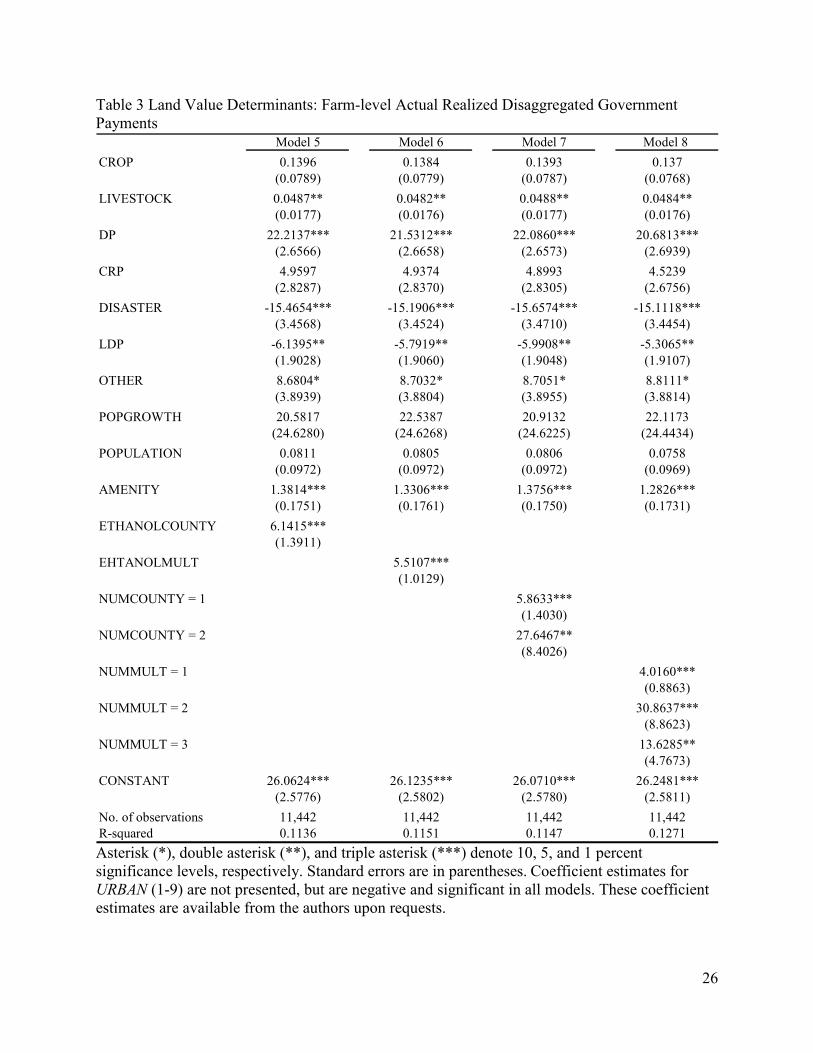
The results for the determinants of farmland values when disaggregated farm-level actual

realized returns are used as regressors are summarized in table 3. The results indicate that the

type of government payments influences the magnitude and size of the effect on farmland values,

confirming previous research (Goodwin, Mishra, and Ortalo-Magné 2003; Goodwin and Mishra

2006; Goodwin, Mishra, and Ortalo-Magné 2011; Patton 2008). Decoupled payments have the

largest impact on farmland values; an additional dollar of decoupled payments per-acre tends to

increase farmland values by approximately $22 per-acre. This suggests a capitalization rate of

19

approximately 4.5 percent. Disaster payments and LDP have a negative impact on farmland

values. Both LDP and disaster payments are received when market returns are low, which may

explain the negative relationships. Again, the results suggest that ethanol facilities have a

positive impact on the value of nearby farmland.

Tables 4 and 5 present the results for the determinants of farmland values when historic

county-level (smoothed) averages are used as independent variables. County-level averages are

used as a proxy for expectations. The capitalization model is based on expected cash flows,

while ARMS data consist of actual values. Actual realize values can differ significantly from

expected values for a variety of reasons, including unexpected adverse market conditions,

drought, disease or discontinuation of a government program. In addition, individual realized

values can vary substantially from year to year. Thus, the county averages may provide a better

measure of true expected values. The results suggest that government payments and ethanol

plants significantly impact farmland values. However, as shown in table 5, when disaggregated

government payments are used, the impacts of ethanol facilities are smaller than in previous

models.

Tables 6-9 present the results for the determinants of rental rates. As shown in table 6, an

additional dollar of government payments per-acre tends to increase rental rates by

approximately $0.32 per-acre. When historic county-level averages are used to proxy for

payment expectations, the results indicate that government payment recipients pass on

approximately 80 percent of the payment to the landlord in the form of higher rental payments,

as shown in table 8. These results are similar to the findings of Goodwin, Mishra, and Ortalo-

Magné (2011). When aggregate government payments are used, ethanol facilities have a positive

impact on rental rates of land in close proximity to the plant; however, when disaggregated

government payments are used, the majority of the coefficients on the ethanol plant variables are

no longer significant. Surprisingly, population growth exhibits a negative effect on rental rates in

most of the models.

Instrumental Variables Regression Results

To further account for measurement error stemming from differences between expected values

and realized values, we employ an instrumental variables approach similar to Goodwin, Mishra,

and Ortalo-Magné (2011). The county-level smoothed averages serve as the instruments. When

government payments are disaggregated, we assume that DP and CRP are exogenous because

20

these payment types are predetermined. Similar results are obtained when these variables are

treated as endogenous. The results are summarized in tables 10-13. As shown in table 10, there is

a positive and significant relationship between government payments and farmland values.

However, the magnitude does not seem plausible. In addition, the majority of the effects of the

ethanol variables are not significant. Similar problems arise when rental rates are analyzed, as

shown in tables 12 and 13. Inspection of the Shea’s partial R-squared values and first-stage F-

statistics (table 14) suggest the instruments may be weak, leading to imprecise and biased

estimates. Given that we use similar instruments to those used by Goodwin, Mishra, and Ortalo-

Magné (2011), we are surprised that the instruments may be problematic. However, the authors

do not discuss the tests conducted to determine the validity of their instruments. In addition, we

recognize that we have only addressed the error-in-variables problems stemming from

measurement error due to differences between expected and actual values and we do not fully

address the endogenous relationship between ethanol plants and farmland. Identifying valid

instruments to address this endogenous relationship presents challenges, which we have not yet

overcome.

Robustness Check Using 2008 Biofuels Supplement Data

As previously stated, the ideal variable to construct to determine the impact of ethanol facilities

on farmland values and rental rates would be the actual distance of the parcel to the closest

ethanol facility. While the ARMS dataset does not contain this information, in 2008 select

respondents were asked to provide additional supplemental data pertaining to biofuels. This

supplemental survey asked respondent to report the distance from the operation’s main storage

facility to the closet ethanol facility. We use the response to this question as a proxy for the

distance from the parcel to the closest ethanol facility. The weighted OLS results are presented in

tables 15 and 16. Models 49 and 52 use farm-level aggregate government payments as

regressors. Unfortunately, there are insufficient observations to conduct the analyses using farm-

level disaggregated government payments because many of the respondents in the sample did not

report disaggregated government payments. The remaining models use historic county-level

averages as the regressors. The results indicate that farmland values are significantly higher

when the parcel is located in close proximity to an operating ethanol production facility.

Farmland values decrease by $26-37 per-acre for every mile between the parcel and the closest

ethanol plant. Rental rates are also significantly impacted by the distance of the parcel from an

21

ethanol facility in models using historic county-level averages as regressors. These models

suggest that for every mile of increased distance rental rates decline by $0.06-0.39.

Conclusions and Implications

While the results are preliminary, they indicate farmland values and rental rates are significantly

higher for parcels located in close proximity to ethanol facilities. Depending on the model, an

ethanol facility in the same county as the parcel increases the value of the parcel by $226-741,

while an ethanol facility in the same county as the parcel may impact rental rates by as much as

$10 per-acre. Furthermore, our findings confirm earlier research that government payments

significantly impact farmland values and rental rates with payment effects dependent on the type

of the payment. The results suggest that U.S. agricultural policies can significantly impact

farmland values.

Ultimately, we would like to be able to answer the question posed in the introduction

regarding whether the recent increase in farmland value is due to changes in government policy

and increased demand or if the increase is due to a speculative bubble. To this end, we use

iterative Chow tests to reveal structural breaks due to the introduction of U.S. ethanol policies

and changes in farm policy regimes. While these results are preliminary, there is evidence that

recent changes in U.S. policies have had a significant impact on farmland uses, prices and rental

rates. We do not report the results of the iterative Chow tests here because we are still refining

the regression analysis. Although our use of historic county-level returns makes some progress

towards correcting the bias associated with the errors-in-variable problems stemming from

differences in actual versus expected values of returns, we have yet to properly instrument for

endogeneity of ethanol facility locations. Identification of a valid instrument is challenging.

Once these identification issues are overcome, a comparison of actual 2011 and predicted

farmland prices generated by the model can be conducted to determine if the current prices are

consistent with fundamentals or if the high prices reflect a speculative bubble. In addition, the

robustness of the model can be examined by comparing changes in farmland values predicted by

the model and basis changes.

In this paper, we ignore differences in ethanol facility capacity levels. Ethanol facilities

vary substantially in terms of their capacity. Future research should also address the impact of

capacity on farmland values and rental rates.

22

References

American Coalition for Ethanol. 2010. http://www.ethanol.org/ Retrieved: June 25, 2010.

Bhaskar, A., and J.C. Beghin. 2010. “Decoupled Farm Payments and the Role of Base Acreage

and Yield Updating Under Uncertainty.” American Journal Agricultural Economics 92:

849-858.

Campbell, J. Y. and R. J. Shiller. 1987. “Cointegration and Tests of Present Value Models.”

Journal of Political Economy 95 (5): 1062-1088.

Clark, J. S., K. K. Klein, and S. J. Thompson. 1993. “Are Subsidies Capitalized into Land

Values? Some Time Series Evidence from Saskatchewan.” Canadian Journal of

Agricultural Economics 75 (1): 147-155.

Goodwin, B.K. and A.K. Mishra. 2006. “Are ‘Decoupled’ Farm Program Payments Really

Decoupled? An Empirical Evaluation.” American Journal Agricultural Economics 88:

73-89.

Goodwin, B. K., A. K. Mishra, and F. N. Ortalo-Magné. 2003. “What's Wrong with Our Models

of Agricultural Land Values?” American Journal of Agricultural Economics, 85(3): 744-

752.

---. 2011. “The Buck Stops Where? The Distribution of Agricultural Subsidies.” NBER Working

Paper. No. 16693.

Henderson, J. and B. Gloy. 2008. “The Impact of Ethanol Plants on Cropland Values In the

Great Plains.” Agricultural Finance Review 69 (1): 36-48.

Kirwan, B.E. 2009 “The Incidence of US Agricultural Subsidies on Farmland Rental Rates.”

Journal of Political Economy 117, 1: 138-164.

Lence, S.H., and A.K. Mishra. 2003. “The Impacts of Different Farm Programs on Cash Rents.”

American Journal Agricultural Economics 85(3):753-61.

McNew, K. and D. Griffith. 2005. “Measuring the Impact of Ethanol Plants on Local Grain

Prices” Review of Agricultural Economics 27 (2): 164-180.

Oppedhal, D. 2011. “The Agricultural Newsletter from the Federal Reserve Bank of Chicago.”

No. 1954, Federal Reserve Bank of Chicago.

Patton M. P., Kostov, S., McErlean, and J. Moss. 2008. “Assessing the Influence of Direct

Payments on the Rental Value of Agricultural Land.” Food Policy 33(5, October):397-

405.

http://www.ethanol.org/

http://www.jstor.org/stable/1245006

http://www.jstor.org/stable/1245006

http://www.jstor.org/action/showPublication?journalCode=amerjagriecon

23

Peckham, J. and J. D. Kropp. Forthcoming. “Decoupled Direct Payments under Base Acreage

and Yield Updating Uncertainty: An Investigation of Agricultural Chemical Use.”

Agricultural and Resource Economics Review.

Renée, Johnson, Coordinator. 2008. The 2008 Farm Bill: A Summary of Major Provisions and

Legislative Action. CRS Report for Congress.

Renewable Fuels Association. 2010. http://www.ethanolrfa.org/bio-refinery-locations/ Retrieved:

June 25 2010.

Tyner, W. E. 2008. “The US Ethanol and Biofuels Boom: Its Origins, Current Status, and Future

Prospects.” BioScience 58 (7):646-653.

U.S. Department of Commerce, Census Bureau, Population Division. 2011. Intercensal

Estimates. Washington, DC, September. http://www.census.gov/popest/data/intercensal

U.S. Department of Agriculture, Economic Research Service (USDA-ERS). 2004. Natural

Amenity Scale. Washington, DC. http://www.ers.usda.gov/Data/NaturalAmenities/

Retrieved: June 25, 2010.

U.S. Department of Agriculture, Economic Research Service (USDA-ERS). 1996. 1996 Farm

Bill. Washington, DC, April.

U.S. Department of Agriculture, Economic Research Service (USDA-ERS). 2002. The 2002

Farm Bill Provisions and Economic Implications. Washington, DC, 22 May.

U.S. Department of Agriculture, National Agricultural Statistics Service (USDA-NASS). 1999. Agricultural Economics and Land Ownership Survey (AELOS). Washington, DC.

http://www.ethanolrfa.org/bio-refinery-locations/

http://www.ers.usda.gov/Data/NaturalAmenities/

Tab

le 1

Var

iabl

e D

efin

ition

s an

d Su

mm

ary

Stat

istic

s

Var

iabl

eD

escr

iptio

nM

ean

Std

Dev

Mea

nSt

d D

evA

CR

ES

Acr

es o

pera

ted

462.

7868

58.1

470

5.32

7457

.48

CO

RN

Acr

es o

f cor

n ha

rves

ted

150.

2329

02.5

126

9.13

3213

.56

AC

RESO

WN

Acr

es o

wne

d24

0.41

4375

.97

232.

9445

77.2

1TEN

UR

EA

CR

ESO

WN

/AC

RES

0.73

5.15

0.38

2.99

LAN

DR

eal f

arm

land

val

ue p

er-a

cre

($/a

cres

own)

2228

.44

184.

9329

88.7

389

4.94

REN

TR

eal r

enta

l rat

e pe

r-ac

re ($

/ren

ted

acre

s)94

.99

96.4

981

.73

5.81

CR

OP

Cro

p sa

les ($

/acr

es)

110.

1865

.96

155.

3817

.49

LIV

EST

OC

KLi

vestoc

k sa

les ($

/acr

es)

100.

3415

2.08

104.

2058

.93

GO

VTot

al g

over

nmen

t pay

men

ts to

ope

rato

r and

land

lord

($/a

cre)

23.3

92.

4326

.27

1.99

DP

Dec

oupl

ed p

aym

ents to

ope

rato

r and

land

lord

($/a

cre)

7.92

0.10

8.20

0.10

CR

PC

RP

paym

ents

to o

pera

tor a

nd la

ndlo

rd ($

/acr

e)4.

621.

510.

990.

43D

ISA

STER

D

isas

ter p

aym

ents to

ope

rato

r and

land

lord

($/a

cre)

2.32

0.70

3.17

0.65

LDP

LDP

to o

pera

tor a

nd la

ndlo

rd ($

/acr

e)5.

641.

268.

221.

23O

TH

ER

O

ther

gov

ernm

ent p

aym

ents to

ope

rato

r and

land

lord

($/a

cre)

1.85

0.98

2.11

0.82

FAR

M A

RC

ES

Tot

al fa

rmla

nd in

cou

nty

2469

78.1

011

3063

.04

2589

42.4

511

1804

.53

AV

G G

OV

Cou

nty

aver

age

gove

rnm

ent p

aym

ents ($

/far

m a

cres

)25

.24

0.25

27.1

80.

25A

VG

DP

Cou

nty

aver

age

deco

uple

d pa

ymen

ts ($

/far

m a

cres

)15

.35

0.06

16.1

60.

06A

VG

CR

PC

ount

y av

erag

e C

RP

paym

ents ($

/far

m a

cres

)4.

150.

043.

730.

04A

VG

DIS

AST

ER

Cou

nty

aver

age

disa

ster

pay

men

ts ($

/far

m a

cres

)4.

740.

044.

820.

04A

VG

LD

PC

ount

y av

erag

e LD

P pa

ymen

ts ($

/far

m a

cres

)9.

390.

059.

780.

05A

VG

OTH

ER

Cou

nty

aver

age

othe

r gov

ernm

ent p

aym

ents ($

/far

m a

cres

)3.

040.

052.

910.

04A

MEN

ITY

Am

enity

z sco

re2.

181.

292.

361.

23ETH

AN

OLC

OU

NTY

Indi

cato

r var

iabl

e (e

than

ol fa

cilit

y in

the

coun

ty)

0.07

2.54

0.09

2.38

ETH

AN

OLM

ULT

Indi

cato

r var

iabl

e (e

than

ol fa

cilit

y in

the

coun

ty o

r nei

ghbo

ring

cou

nty)

0.12

3.20

0.15

3.00

NU

MC

OU

NTY

Num

ber o

f eth

anol

faci

litie

s in

the

coun

ty0.

072.

650.

092.

49N

UM

MU

LTN

umbe

r of e

than

ol fa

cilit

ies in

the

coun

ty0.

133.

710.

173.

57PO

PGR

OW

TH

Ann

ual p

opul

atio

n gr

owth

rate

0.00

0.01

0.00

0.01

POPU

LATIO

NR

atio

of c

ount

y po

pula

tion

in fa

rm a

cres

0.45

5.82

0.46

5.73

DIS

TA

NC

ED

ista

nce

from

sto

rage

faci

lity

to c

lose

st e

than

ol fa

cilit

y25

.74

19.3

325

.01

18.0

4

Land

val

ue sam

ple

Ren

tal r

ate

sam

ple

Mea

ns c

alcu

late

d us

ing

AR

MS

data

are

wei

ghte

d. M

eans

cal

cula

ted

from

oth

er d

ata

sour

ces ar

e un

wei

ghte

d.

Table 2 Land Value Determinants: Farm-level Actual Realized Aggregate Government Payments

Model 1 Model 2 Model 3 Model 4

CROP 0.1921 0.188 0.1916 0.1857(0.1023) (0.0997) (0.1020) (0.0984)

LIVESTOCK 0.0330* 0.0325* 0.0332* 0.0325*(0.0141) (0.0139) (0.0141) (0.0138)

GOV 2.9163*** 2.7882*** 2.9293*** 2.8191***(0.7765) (0.7736) (0.7764) (0.7725)

POPGROWTH 9.284 14.5617 9.5693 15.218(20.1192) (20.0866) (20.1141) (20.0447)

POPULATION -0.0054 -0.0056 -0.0056 -0.0066(0.0325) (0.0325) (0.0325) (0.0324)

AMENITY 1.9198*** 1.7921*** 1.9094*** 1.7406***(0.1403) (0.1400) (0.1402) (0.1392)

ETHANOLCOUNTY 7.4058***(0.7649)

ETHANOLMULT 7.2782***(0.5713)

NUMCOUNTY = 1 7.0832***(0.7776)

NUMCOUNTY = 2 18.6952***(3.2126)

NUMMULT = 1 6.1180***(0.5617)

NUMMULT = 2 18.1549***(2.4291)

NUMMULT = 3 11.5833(6.9849)

CONSTANT 31.7185*** 31.8467*** 31.7296*** 31.9173***(2.4455) (2.4487) (2.4458) (2.4494)

No. of observations 28,204 28,204 28,204 28,204R-squared 0.0902 0.095 0.0909 0.0994

Asterisk (*), double asterisk (**), and triple asterisk (***) denote 10, 5, and 1 percent significance levels, respectively. Standard errors are in parentheses. Coefficient estimates for URBAN (1-9) are not presented, but are negative and significant in all models. These coefficient estimates are available from the authors upon requests.

26

Table 3 Land Value Determinants: Farm-level Actual Realized Disaggregated Government Payments


CROP 0.1396 0.1384 0.1393 0.137(0.0789) (0.0779) (0.0787) (0.0768)

LIVESTOCK 0.0487** 0.0482** 0.0488** 0.0484**(0.0177) (0.0176) (0.0177) (0.0176)

DP 22.2137*** 21.5312*** 22.0860*** 20.6813***(2.6566) (2.6658) (2.6573) (2.6939)

CRP 4.9597 4.9374 4.8993 4.5239(2.8287) (2.8370) (2.8305) (2.6756)

DISASTER -15.4654*** -15.1906*** -15.6574*** -15.1118***(3.4568) (3.4524) (3.4710) (3.4454)

LDP -6.1395** -5.7919** -5.9908** -5.3065**(1.9028) (1.9060) (1.9048) (1.9107)

OTHER 8.6804* 8.7032* 8.7051* 8.8111*(3.8939) (3.8804) (3.8955) (3.8814)

POPGROWTH 20.5817 22.5387 20.9132 22.1173(24.6280) (24.6268) (24.6225) (24.4434)

POPULATION 0.0811 0.0805 0.0806 0.0758(0.0972) (0.0972) (0.0972) (0.0969)

AMENITY 1.3814*** 1.3306*** 1.3756*** 1.2826***(0.1751) (0.1761) (0.1750) (0.1731)


EHTANOLMULT 5.5107***(1.0129)

NUMCOUNTY = 1 5.8633***(1.4030)

NUMCOUNTY = 2 27.6467**(8.4026)

NUMMULT = 1 4.0160***(0.8863)

NUMMULT = 2 30.8637***(8.8623)

NUMMULT = 3 13.6285**(4.7673)

CONSTANT 26.0624*** 26.1235*** 26.0710*** 26.2481***(2.5776) (2.5802) (2.5780) (2.5811)



27

Table 4 Land Value Determinants: Historic County-level Average Aggregate Government Payments


CROP 0.1695 0.1666 0.1691 0.1646(0.0900) (0.0881) (0.0897) (0.0869)

LIVESTOCK 0.0305* 0.0302* 0.0307* 0.0302*(0.0131) (0.0129) (0.0131) (0.0128)

AVG GOV 36.7712*** 36.1882*** 36.7407*** 36.0030***(2.6029) (2.5835) (2.6030) (2.5774)

POPGROWTH 47.1548* 51.0004* 47.3675* 51.3654*(20.6081) (20.5515) (20.6059) (20.5129)

POPULATION -0.0375 -0.0371 -0.0376 -0.0379(0.0343) (0.0342) (0.0343) (0.0343)

AMENITY 1.3337*** 1.2385*** 1.3253*** 1.1957***(0.1619) (0.1601) (0.1619) (0.1594)


ETHANOLMULT 6.1241***(0.5508)

NUMCOUNTY = 1 6.1547***(0.7543)

NUMCOUNTY = 2 16.8639***(3.0164)

NUMMULT = 1 5.0547***(0.5437)

NUMMULT = 2 16.1443***(2.3764)

NUMMULT = 3 12.1709(6.3686)

CONSTANT 22.2506*** 22.4926*** 22.2709*** 22.6128***(2.5031) (2.5044) (2.5035) (2.5044)



28

Table 5 Land Value Determinants: Historic County-level Average Disaggregated Government Payments


CROP 0.1393 0.1383 0.1392 0.1374(0.0716) (0.0710) (0.0716) (0.0704)

LIVESTOCK 0.0287* 0.0286* 0.0288* 0.0286*(0.0126) (0.0124) (0.0126) (0.0124)

AVG DP 95.8399*** 94.4277*** 95.6324*** 93.5300***(5.5314) (5.5413) (5.5297) (5.5200)

AVG CRP 13.6243** 14.6344*** 13.6631** 15.7918***(4.2481) (4.2306) (4.2472) (4.2158)

AVG DISASTER -25.7591*** -24.1288*** -25.4049*** -22.2961**(7.2746) (7.2936) (7.2765) (7.3295)

AVG LDP 12.5433*** 12.3205*** 12.4984*** 12.2241***(2.5373) (2.5307) (2.5353) (2.5267)

AVG OTHER 47.0202*** 45.7096*** 46.8735*** 44.5928***(8.8315) (8.7288) (8.8298) (8.6408)

POPGROWTH 43.2169* 46.1248* 43.3365* 47.0139*(19.5118) (19.5240) (19.5114) (19.5281)

POPULATION -0.0393 -0.0381 -0.0393 -0.0377(0.0310) (0.0309) (0.0310) (0.0308)

AMENITY 0.6232*** 0.5785*** 0.6212*** 0.5513***(0.1552) (0.1539) (0.1551) (0.1528)


EHTANOLMULT 4.0072***(0.5838)

NUMCOUNTY = 1 4.1936***(0.7643)

NUMCOUNTY = 2 9.8482**(3.0037)

NUMMULT = 1 3.2122***(0.5673)

NUMMULT = 2 12.1471***(2.4665)

NUMMULT = 3 7.4945(5.8961)

CONSTANT 19.1626*** 19.3362*** 19.1855*** 19.4276***(2.4987) (2.5004) (2.4987) (2.5003)



29

Table 6 Rental Rate Determinants: Farm-level Actual Realized Aggregate Government Payments


CROP 0.0907*** 0.0898*** 0.0906*** 0.0894***(0.0071) (0.0070) (0.0070) (0.0070)

LIVESTOCK 0.0057** 0.0057** 0.0057** 0.0056**(0.0022) (0.0022) (0.0022) (0.0022)

GOV 0.3171*** 0.3195*** 0.3179*** 0.3202***(0.0382) (0.0382) (0.0382) (0.0382)

POPGROWTH -2.5951*** -2.5287*** -2.5886*** -2.5131***(0.7158) (0.7154) (0.7157) (0.7154)

POPULATION -0.0007 -0.0006 -0.0007 -0.0007(0.0061) (0.0061) (0.0061) (0.0061)

AMENITY 0.0717*** 0.0698*** 0.0716*** 0.0691***(0.0067) (0.0068) (0.0067) (0.0068)


ETHANOLMULT 0.1071***(0.0164)

NUMCOUNTY = 1 0.0987***(0.0197)

NUMCOUNTY = 2 0.2339*(0.0942)

NUMMULT = 1 0.0931***(0.0167)

NUMMULT = 2 0.2166***(0.0424)

NUMMULT = 3 0.2247*(0.0936)

CONSTANT 0.3960*** 0.3996*** 0.3963*** 0.4017***(0.0477) (0.0477) (0.0477) (0.0477)



30

Table 7 Rental Rate Determinants: Farm-level Actual Realized Disaggregated Government Payments


CROP 0.0830*** 0.0827*** 0.0829*** 0.0822***(0.0085) (0.0085) (0.0085) (0.0085)

LIVESTOCK 0.0071 0.0071 0.0071 0.0071(0.0041) (0.0041) (0.0041) (0.0041)

DP 0.6194*** 0.6140*** 0.6193*** 0.6087***(0.1027) (0.1026) (0.1027) (0.1025)

CRP -0.4933* -0.4871* -0.4943* -0.4865*(0.2190) (0.2179) (0.2189) (0.2172)

DISASTER 0.5195** 0.5242** 0.5207** 0.5275**(0.1785) (0.1785) (0.1785) (0.1786)

LDP 0.2096** 0.2129** 0.2107** 0.2160**(0.0788) (0.0788) (0.0788) (0.0788)

OTHER 0.3728 0.3731 0.3729 0.3735(0.2633) (0.2631) (0.2634) (0.2636)

POPGROWTH -2.3808* -2.3654* -2.3763* -2.3631*(0.9826) (0.9829) (0.9827) (0.9835)

POPULATION 0.0029 0.003 0.0029 0.003(0.0096) (0.0096) (0.0096) (0.0095)

AMENITY 0.0623*** 0.0617*** 0.0622*** 0.0612***(0.0093) (0.0094) (0.0093) (0.0094)

ETHANOLCOUNTY 0.0362(0.0280)

EHTANOLMULT 0.0457*(0.0226)

NUMCOUNTY = 1 0.0327(0.0281)

NUMCOUNTY = 2 0.331(0.1875)

NUMMULT = 1 0.0327(0.0222)

NUMMULT = 2 0.2599*(0.1246)

NUMMULT = 3 0.2317(0.1427)

CONSTANT 0.3180*** 0.3194*** 0.3182*** 0.3214***(0.0608) (0.0608) (0.0608) (0.0608)



31

Table 8 Rental Rate Determinants: Historic County-level Average Aggregate Government Payments


CROP 0.0836*** 0.0830*** 0.0835*** 0.0827***(0.0066) (0.0065) (0.0066) (0.0065)

LIVESTOCK 0.0055* 0.0055* 0.0055* 0.0054*(0.0022) (0.0022) (0.0022) (0.0022)

AVG GOV 0.8165*** 0.8094*** 0.8163*** 0.8078***(0.0771) (0.0765) (0.0771) (0.0765)

POPGROWTH -2.1299** -2.0922** -2.1267** -2.0814**(0.6685) (0.6678) (0.6685) (0.6680)

POPULATION -0.0023 -0.0023 -0.0023 -0.0023(0.0061) (0.0060) (0.0061) (0.0060)

AMENITY 0.0721*** 0.0709*** 0.0720*** 0.0703***(0.0068) (0.0068) (0.0068) (0.0068)


ETHANOLMULT 0.0774***(0.0157)

NUMCOUNTY = 1 0.0729***(0.0190)

NUMCOUNTY = 2 0.1603(0.0933)

NUMMULT = 1 0.0653***(0.0160)

NUMMULT = 2 0.1710***(0.0419)

NUMMULT = 3 0.2044**(0.0746)

CONSTANT 0.2548*** 0.2595*** 0.2551*** 0.2618***(0.0460) (0.0460) (0.0460) (0.0460)



32

Table 9 Rental Rate Determinants: Historic County-level Average Disaggregated Government Payments


CROP 0.0681*** 0.0680*** 0.0681*** 0.0679***(0.0057) (0.0057) (0.0057) (0.0057)

LIVESTOCK 0.0052* 0.0052* 0.0052* 0.0052*(0.0022) (0.0021) (0.0022) (0.0021)

AVG DP 3.1195*** 3.1086*** 3.1214*** 3.1001***(0.2102) (0.2107) (0.2106) (0.2109)

AVG CRP 0.0191 0.032 0.0192 0.0436(0.1776) (0.1785) (0.1776) (0.1789)

AVG DISASTER 0.5407* 0.5578* 0.5372* 0.5773*(0.2692) (0.2698) (0.2695) (0.2705)

AVG LDP 0.4343*** 0.4315*** 0.4349*** 0.4314***(0.0937) (0.0936) (0.0936) (0.0937)

AVG OTHER 0.2502 0.2362 0.2514 0.2236(0.1639) (0.1630) (0.1640) (0.1629)

POPGROWTH -1.1381 -1.1234 -1.1393 -1.1118(0.6475) (0.6480) (0.6476) (0.6482)

POPULATION 0.0001 0.0001 0.0001 0.0001(0.0056) (0.0056) (0.0056) (0.0056)

AMENITY 0.0385*** 0.0382*** 0.0385*** 0.0378***(0.0068) (0.0069) (0.0068) (0.0069)


EHTANOLMULT 0.0265(0.0156)

NUMCOUNTY = 1 0.0259(0.0186)

NUMCOUNTY = 2 -0.0128(0.0935)

NUMMULT = 1 0.0194(0.0157)

NUMMULT = 2 0.0856*(0.0418)

NUMMULT = 3 0.0932(0.0671)

CONSTANT 0.0167 0.0184 0.0165 0.0196(0.0499) (0.0499) (0.0499) (0.0499)



33

Table 10 Land Value Determinants: Instrumental Variables and Aggregate Government Payments


CROP 0.1435* 0.1432* 0.1428* 0.1402*(0.0674) (0.0672) (0.0670) (0.0657)

LIVESTOCK 0.0577*** 0.0577*** 0.0579*** 0.0577***(0.0159) (0.0158) (0.0159) (0.0158)

GOV 234.7195*** 234.1720*** 234.3762*** 233.0032***(28.2130) (28.5289) (28.1571) (28.3860)

POPGROWTH 315.2306*** 315.4965*** 315.2132*** 314.7668***(67.6083) (67.4492) (67.5048) (67.1062)

POPULATION 0.2113* 0.2107* 0.2106* 0.2082*(0.1024) (0.1022) (0.1021) (0.1012)

AMENITY -9.5823*** -9.5679*** -9.5811*** -9.5768***(1.5251) (1.5284) (1.5232) (1.5242)


ETHANOLMULT 1.6008(1.8800)

NUMCOUNTY = 1 1.7438(2.3771)

NUMCOUNTY = 2 20.6178(11.1544)

NUMMULT = 1 0.0918(1.9641)

NUMMULT = 2 14.6696**(4.7170)

NUMMULT = 3 44.5506***(8.7736)

CONSTANT -5.2107 -5.1167 -5.1347 -4.8289(7.0571) (7.0853) (7.0455) (7.0499)

No. of observations 28,204 28,204 28,204 28,204


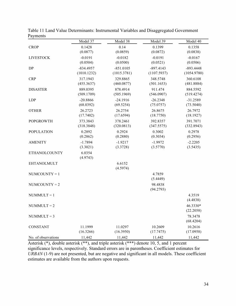
34

Table 11 Land Value Determinants: Instrumental Variables and Disaggregated Government Payments


CROP 0.1428 0.14 0.1399 0.1358(0.0877) (0.0859) (0.0872) (0.0838)

LIVESTOCK -0.0191 -0.0182 -0.0191 -0.0167(0.0504) (0.0500) (0.0521) (0.0506)

DP -834.4957 -851.0105 -897.4143 -893.4448(1010.1232) (1015.3781) (1107.5937) (1054.9780)

CRP 317.1943 329.8865 348.5748 360.6108(455.3637) (460.0877) (501.1653) (481.8884)

DISASTER 889.0395 878.4914 911.474 884.5592(509.1709) (505.1969) (546.0907) (519.4274)

LDP -20.8866 -24.1916 -26.2348 -31.2589(68.0392) (69.5254) (75.0757) (73.5040)

OTHER 26.2723 26.2754 26.8675 26.7972(17.7402) (17.6594) (18.7750) (18.1927)

POPGROWTH 373.3843 378.2461 392.8357 391.7071(318.3848) (320.0813) (347.5575) (332.8943)

POPULATION 0.2892 0.2924 0.3002 0.2978(0.2862) (0.2880) (0.3034) (0.2956)

AMENITY -1.7894 -1.9217 -1.9972 -2.2205(3.3021) (3.3728) (3.5770) (3.5435)



NUMCOUNTY = 1 4.7859(5.4449)

NUMCOUNTY = 2 98.4838(94.2793)

NUMMULT = 1 4.3519(4.4838)

NUMMULT = 2 46.3330*(22.2058)

NUMMULT = 3 78.3478(68.4204)

CONSTANT 11.1999 11.0297 10.2609 10.2616(16.3266) (16.3950) (17.7475) (17.0958)



35

Table 12 Rental Rate Determinants: Instrumental Variables and Aggregate Government Payments


CROP 0.0667*** 0.0650*** 0.0661*** 0.0643***(0.0108) (0.0106) (0.0108) (0.0107)

LIVESTOCK -0.0026 -0.0024 -0.0025 -0.0024(0.0039) (0.0037) (0.0039) (0.0037)

GOV 8.1559*** 7.8371*** 8.1309*** 7.8237***(1.8476) (1.7262) (1.8357) (1.7230)

POPGROWTH 8.6390* 8.2557* 8.6447* 8.2609*(3.5827) (3.4027) (3.5702) (3.3984)

POPULATION 0.0139 0.0135 0.0138 0.0134(0.0116) (0.0112) (0.0115) (0.0112)

AMENITY -0.2587** -0.2498*** -0.2588** -0.2507***(0.0798) (0.0753) (0.0795) (0.0754)


ETHANOLMULT 0.1582**(0.0569)

NUMCOUNTY = 1 0.0267(0.0735)

NUMCOUNTY = 2 1.0835***(0.2962)

NUMMULT = 1 0.1287*(0.0572)

NUMMULT = 2 0.3583*(0.1548)

NUMMULT = 3 1.1856**(0.4115)

CONSTANT -1.3247** -1.2428** -1.3160** -1.2353**(0.4480) (0.4194) (0.4448) (0.4182)



36

Table 13 Rental Rate Determinants: Instrumental Variables and Disaggregated Government Payments


CROP 0.0867*** 0.0853*** 0.0861*** 0.0844***(0.0148) (0.0151) (0.0151) (0.0155)

LIVESTOCK 0.0073 0.0085 0.0077 0.0089(0.0160) (0.0168) (0.0165) (0.0174)

DP -12.4043 -13.5887 -13.0284 -14.3434(18.7893) (19.6018) (19.3333) (20.2344)

CRP 7.0563 7.5825 7.3165 7.9531(7.4176) (7.7334) (7.6364) (7.9875)

DISASTER 1.9715 1.5192 1.8327 1.4006(5.6766) (5.9032) (5.8472) (6.0784)

LDP -0.7444 -0.8628 -0.7963 -0.9436(1.5715) (1.6416) (1.6189) (1.6971)

OTHER 0.0258 0.0395 0.0273 0.0579(0.3526) (0.3720) (0.3625) (0.3850)

POPGROWTH 2.8405 3.1377 2.9967 3.3812(4.4247) (4.6187) (4.5409) (4.7750)

POPULATION 0.0073 0.0077 0.0074 0.0079(0.0115) (0.0116) (0.0116) (0.0117)

AMENITY 0.028 0.0266 0.0276 0.0246(0.0195) (0.0209) (0.0202) (0.0217)



NUMCOUNTY = 1 0.0919 0.0919(0.0908) (0.0908)

NUMCOUNTY = 2 0.6544*(0.2611)

NUMMULT = 1 0.0849(0.0645)

NUMMULT = 2 0.389(0.2450)

NUMMULT = 3 1.1539(0.9395)

CONSTANT 0.0879 0.082 0.0843 0.0757(0.1847) (0.1972) (0.1912) (0.2061)



Tab

le 1

4 Tes

ts fo

r Wea

k In

stru

men

ts

AV

G

GO

VA

VG

D

ISA

STER

AV

GLD

PA

VG

O

TH

ER

AV

G

GO

VA

VG

D

ISA

STER

AV

GLD

PA

VG

O

TH

ER

Mod

el 3

351

.811

70.

0068

Mod

el 3

450

.782

70.

0066

Mod

el 3

551

.870

30.

0068

Mod

el 3

650

.802

90.

0066

Mod

el 3

719

.224

319

.647

44.

4104

20.

0005

0.00

080.

0005

Mod

el 3

819

.242

219

.344

84.

4462

0.00

040.

0008

0.00

05M

odel

39

19.3

381

19.4

176

4.40

874

0.00

040.

0007

0.00

05M

odel

40

19.2

433

18.9

205

4.43

782

0.00

040.

0007

0.00

05M

odel

41

15.2

413

0.00

28M

odel

42

16.0

109

0.00

30M

odel

43

15.3

361

0.00

28M

odel

44

16.0

116

0.00

30M

odel

45

22.5

757

32.6

694

12.7

822

0.00

020.

0003

0.00

16M

odel

46

22.3

208

32.1

141

12.7

300

0.00

020.

0003

0.00

16M

odel

47

22.5

125

32.4

543

12.7

313

0.00

020.

0003

0.00

16M

odel

48

22.1

617

31.6

066

12.4

979

0.00

020.

0003

0.00

17

Firs

t-St

age

F-stat

isic

Shea

's pa

rtia

l R-s

quar

ed

Table 15 Land Value Determinants: Robustness Check Model 49 Model 50 Model 51

CROP 1.3782* 0.8950** 0.8437**(0.5760) (0.3416) (0.3203)

LIVESTOCK -0.2828 -1.0246 -0.9416(0.8304) (0.7045) (0.7279)

GOV 4.0838 156.6502***(12.8794) (32.5887)

DP 211.4380***(55.2506)

CRP 186.1446(94.4096)

DISASTER 35.1403(443.7852)

LDP 291.0618(176.5233)

OTHER 272.7921(334.1481)

POPGROWTH 980.0605* 1297.1270** 1278.7534**(470.6745) (397.3041) (424.2238)

POPULATION 7.8384 6.0199 5.1241(6.5595) (4.6243) (4.1223)

AMENITY 2.7065 -0.951 -0.7856(2.5809) (1.9434) (2.4373)

DISTANCE -0.2638** -0.3366*** -0.3737***(0.0888) (0.0730) (0.0814)

CONSTANT 29.1216 -10.5071 -13.1047(16.0154) (17.3324) (20.7679)

No. of observations 152 152 152R-squared 0.2563 0.3935 0.4148 Asterisk (*), double asterisk (**), and triple asterisk (***) denote 10, 5, and 1 percent significance levels, respectively. Standard errors are in parentheses. Coefficient estimates for URBAN (1-9) are not presented, but are negative and significant in all models. These coefficient estimates are available from the authors upon requests.

39

Table 16 Rental Rate Determinants: Robustness Check Model 52 Model 53 Model 54

CROP 0.0346** 0.0299*** 0.0275**(0.0110) (0.0081) (0.0082)

LIVESTOCK -0.0002 -0.0004*** -0.0004***(0.0001) (0.0001) (0.0001)

GOV 0.6181* 4.4249***(0.2866) (0.5003)

DP 6.0444***(1.1646)

CRP 3.9413*(1.6391)

DISASTER 13.8681(9.8103)

LDP -3.1328(4.2435)

OTHER 8.7986(6.3934)

POPGROWTH -7.6316 6.2444 3.3664(6.2282) (4.8164) (5.5149)

POPULATION -0.0469 0.044 -0.0417(0.0636) (0.0503) (0.0708)

AMENITY 0.0239 -0.0481 -0.0507(0.0668) (0.0488) (0.0487)

DISTANCE -0.0006 -0.0029** -0.0039**(0.0016) (0.0011) (0.0013)

CONSTANT 0.5847* -0.6846* -0.7387(0.2510) (0.2827) (0.3781)

No. of observations 130 130 130R-squared 0.3821 0.5780 0.5945 Asterisk (*), double asterisk (**), and triple asterisk (***) denote 10, 5, and 1 percent significance levels, respectively. Standard errors are in parentheses. Coefficient estimates for URBAN (1-9) are not presented, but are negative and significant in all models. These coefficient estimates are available from the authors upon requests.

Impacts of U.S. Agricultural and Ethanol Policies on...

Documents

Transcript of Impacts of U.S. Agricultural and Ethanol Policies on...