i

United States Department of Agriculture

U.S. Ethanol: An Examination of Policy, Production, Use, Distribution, and Market Interactions

Editors

James A. Duffield U.S. Department of Agriculture Office of the Chief Economist

Office of Energy Policy and New Uses

Robert Johansson U.S. Department of Agriculture Office of the Chief Economist

Seth Meyer U.S. Department of Agriculture Office of the Chief Economist

World Agricultural Outlook Board

Office of Energy Policy and New Uses Office of the Chief Economist

U.S. Department of Agriculture

ii

Access this report online: http://www.usda.gov/oce/energy/index.htm Use of commercial and trade names does not imply approval or constitute endorsement by USDA. The U.S. Department of Agriculture (USDA) prohibits discrimination in all its programs and activities on the basis of race, color, national origin, age, disability, and, where applicable, sex, marital status, familial status, parental status, religion, sexual orientation, genetic information, political beliefs, reprisal, or because all or a part of an individual’s income is derived from any public assistance program. (Not all prohibited bases apply to all programs.) Persons with disabilities who require alternative means for communication of program information (Braille, large print, audiotape, etc.) should contact USDA’s TARGET Center at (202) 720-2600 (voice and TDD). To file a complaint of discrimination write to USDA, Director, Office of Civil Rights, 1400 Independence Avenue, S.W., Washington, D.C. 20250-9410 or call (800) 795-3272 (voice) or (202) 720-6382 (TDD). USDA is an equal opportunity provider and employer. September 2015

iii

Contents

Foreword IV

Acknowledgements V

Chapter 1. Effects of Policy on Ethanol Industry Growth 1 James A. Duffield and Irene Xiarchos, USDA Office of Energy Policy and New Uses Chapter 2. Interaction Between Ethanol, Crop, and Livestock Markets 10 Peter Riley, USDA, Farm Service Agency Chapter 3. Managing the U.S. Corn Transportation and Storage System 41 Marina Denicoff, USDA, Agricultural Marketing Service; and Peter Riley, USDA, Farm Service Agency Chapter 4. Corn Ethanol Processing Technology, Cost of Production, and 45 Profitability Paul Gallagher, Department of Economics, Iowa State University Chapter 5. Ethanol Distribution, Trade Flows, and Shipping Costs 49 Paul Gallagher, Department of Economics, Iowa State University; and Marina Denicoff, USDA, Agricultural Marketing Service Chapter 6. Demand for Ethanol Blending 56 Anthony Radich, U.S. Energy Information Administration (EIA) Chapter 7. Potential for Higher Ethanol Blends in Finished Gasoline 60 Paul Gallagher, Department of Economics, Iowa State University and James A. Duffield, USDA, Office of Energy Policy and New Uses Chapter 8. Policy Challenges and the Future Direction of Biofuels 65 James A. Duffield and Harry Baumes, USDA Office of Energy Policy and New Uses References 72 Appendix 80

iv

Foreword

Inquiries concerning ethanol from a broad spectrum of people, including U.S. policymakers, international leaders, and various interest groups, led to the commissioning of this report. It intends to bring clarity to the complex interaction of ethanol production with agricultural markets and government policies. While there are many other ethanol studies available, this report is unique in that it centers on the pivotal role that ethanol plays in the crop and feed markets. In addition, it provides detailed and current analyses on ethanol production costs, profitability, processing technology, and the infrastructure that supports the industry. Also examined are the economics of blending ethanol into gasoline for octane enhancement and to meet clean air regulations. Federal and State policies are described to illustrate the importance of energy legislation, environmental regulation, and farm policy to the development of the ethanol industry. The authors of this report come from the U.S. Department of Agriculture (USDA), the U.S. Energy Information Administration (EIA), and the Economics Department at Iowa State University (ISU). The USDA agencies contributing to this report include Farm Service Agency (FSA), Agricultural Marketing Service (AMS), and the Office of the Chief Economist (OCE). FSA used USDA's extensive crop and livestock survey data to show changes in the production of corn, other feed grains, forage feeds, and animal inventories over time. These changes relate to a number of factors, including the adjustment of agricultural markets to the increasing demand for corn ethanol. AMS supplied logistical information on the transportation network for U.S. corn and ethanol. OCE provided oversight and coordination and contributed to the policy sections of this report. EIA provided technical and regulatory information on blending ethanol into gasoline. The current conditions that are preventing significant volumes of higher ethanol blends, such as E15 and E85, from being used in the U.S. auto fleet were also reported. Iowa State University broadened the scope of this report in several areas, including ethanol costs of production, profitability, regional trade flows, transportation costs, ethanol pricing, fuel economy, and factors affecting ethanol demand. The U.S. ethanol industry appears to be at a critical juncture, and this report identifies the many factors leading to its current conditions and presents the challenges of moving the biofuels industry forward. I am grateful to the authors, editors, reviewers, and others who made contributions to this report. Robert Johansson Chief Economist U.S. Department of Agriculture

v

Acknowledgements

This report was conceptualized by USDA's Office of the Chief Economist, which directed the Office of Energy Policy and New Uses (OEPNU) to coordinate the selection of authors, editing, and review process. In addition to the authors, many others played key roles in making this publication possible. A special thanks to Ray Bridge, who served as technical editor and content advisor. Much gratitude is extended to Linwood Hoffman and Tom Capehart from USDA's Economic Research Service, who provided insightful reviews, edits, and suggestions. Jerry Norton from the World Agricultural Outlook Board provided timely data and graphics for the report. Brenda Chapin, OCE's Information Officer, guided the manuscript through the Departmental clearance process. Jennifer Lohr, OCE's Web Manager, prepared the report for the OCE website. Finally, this report is dedicated to the remembrance of Roger Conway (1951-2014), who served as Director of the Office of Energy Policy and New Uses (OEPNU) from 1990 to 2009. Through Conway's efforts, OEPNU became a more productive, relevant, and rewarding place to work.

1

Chapter 1: Effects of Policy on Ethanol Industry Growth James A. Duffield Irene Xiarchos The corn ethanol industry is the largest biofuel producer in the United States, with production increasing from about 1.6 billion gallons in 2000 to just over 14 billion gallons in 2014 (Figure 1.1). The growing ethanol market has benefited crop farmers by boosting corn and other agricultural commodity prices, which in turn has stimulated economic activity in rural areas. Besides benefiting portions of the farm sector, ethanol has become an important component of U.S. environmental policy and a significant source of motor fuel. There are other factors behind ethanol’s remarkable growth rate, but the industry owes much of it success to government policies and regulations.

Figure 1.1. Historical ethanol production and policies effecting growth since 2000*

* Year 2015 is RFS2 volume requirement of 15 billion gallons. Sources: Renewable Fuels Association and National Agricultural Law Center. Note: RFS2 is the Renewable Fuel Standard-2; VEETC is the Volumetric Ethanol Excise Tax Credit; EPAct is the Energy Policy Act; MTBE is Methyl Tertiary Butyl Ether. Motivated by gasoline shortages during the energy crises of the 1970s, policymakers began a long history of passing legislation to foster ethanol growth, mainly in the form of tax credits and other economic incentives (Duffield et al, 2008). While ethanol has many desirable characteristics, particularly as an octane additive, the infant industry struggled in the early years to compete in the gasoline market. Thus, to encourage more investment in the fledgling industry, ethanol production received its first tax credit in 1978 (Appendix table 1). Ethanol advocates argued that government support for ethanol was justified because it provided public benefits in

0

2,000

4,000

6,000

8,000

10,000

12,000

14,000

16,000

RFS2 phase-in implemented in 2010

2008 Farm Bill reduced VEETC to $0.45 in 2009, which eventually expired at the end of 2011

EPAct 2005 created the RFS that mandated yearly ethanol production up to 7.5 billion gallons in 2012

In 2004, the $0.51 VEETC was created and set to expire in 2010

In 1999, California passed law to phase out MTBE

Million gallons

2

terms of reduced air pollution, reduced dependence on unreliable sources of oil, and increased economic growth in rural areas. Policymakers from the Corn Belt States particularly had interest in creating new markets for farmers because, at that time, U.S. agriculture suffered from price volatility and frequently experienced low commodity prices caused by crop surpluses. To further assist U.S. farmers, a 2.5-percent ad valorem tariff and an import duty on ethanol of $0.54 per gallon were established in 1980 (Yacobucci). Duty-free treatment for ethanol was granted to 22 Caribbean Basin countries and territories in January1984, under the Caribbean Basin Initiative (Appendix table 1). Another approach used by Congress to increase ethanol demand occurred in 1988 with the passage of the Alternative Motor Fuels Act that provided credits to automakers towards meeting their corporate average fuel efficiency (CAFE) standards for manufacturing alternative-fueled vehicles, including flexible-fueled vehicles (FFV). FFVs can be fueled by gasoline, or any combination of ethanol and gasoline, up to a blend containing 85 percent ethanol and 15 percent gasoline (E85).

Tax credits and other energy-related policies helped ethanol production grow at a slow, but steady, pace throughout the 1970s and 1980s. However, ethanol production received a major boost in the 1990s, when environmental policies began to play a larger role in the industry’s development. The first environmental policy to have a major effect on renewable energy was the Clean Air Act Amendments of 1990 (CAA). Provisions of the CAA established the Oxygenated Fuels Program and the Reformulated Gasoline (RFG) Program to control carbon monoxide and ozone problems in certain urban areas around the country that were judged to be in “non-attainment.” Both program fuels required the addition of oxygen compounds to gasoline, and blending ethanol became a popular method for gasoline producers to meet the new oxygen requirements mandated by the CAA (Unzelman).

The oxygenate requirement increased the demand for ethanol significantly, but the preferred oxygenate at the time was a petroleum product called methyl tertiary butyl ether (MTBE). To help ethanol compete with MTBE, the ethanol excise tax exemption was modified in the Energy Policy Act of 1992 (EPAct). The EPAct extended the fuel tax exemption and the blender’s income tax credit to two additional blend rates containing less than 10 percent ethanol, effective January 1, 1993 (National Agricultural Law Center). These additional blends were added to encourage blending of ethanol to make oxygenated gasoline in the Oxygenated Fuels Program, requiring 7.7 percent ethanol, and in the RFG Program, which requires 5.7 percent ethanol. Thanks to these new tax provisions, the RFG market quickly became the largest market for ethanol production. This act also required Federal agencies to purchase a certain percentage of alternative-fuel vehicles, such as electric vehicles and vehicles fueled by propane, natural gas, and FFVs. FFVs became a popular choice for meeting these requirements because there was a large selection of FFV models available, since automobile manufacturers earn CAFE credits for producing them. However, the requirements for earning these credits were recently modified under the so called CAFE/GHG rule that combined fuel economy standards with greenhouse gas (GHG) emission standards for light-duty vehicles. Starting with 2016 models, CAFE credits for FFVs will be phased out, and after model year 2019, no FFV credits will be available for CAFE compliance (Federal Register, 2010b). After 2019, the only credits available for FFVs will be for GHG compliance, but FFVs must actually use E85 before manufacturers can receive the credit.

3

Another environmental rule provided a major boost for ethanol production in 1999, when the Governor of California announced that the State would ban the use of MTBE, because of water contamination, at the earliest possible date (McCarthy and Tiemann). The California Air Resources Board (CARB) made a formal request to EPA for a waiver from the requirement to use oxygenates in reformulated gasoline so refineries would not be forced to add oxygenates to their gasoline. More than 2 years later, on June 12, 2001, EPA denied California’s request. Without a waiver, gasoline sold in nonattainment areas in the State were required to use the only other oxygenate available, which was ethanol. By 2003, California began to gradually phase out MTBE in favor of ethanol. At least 24 other States followed California’s lead, and MTBE rapidly began to lose market share to ethanol throughout much of the country (McCarthy and Tiemann). More details on State ethanol policies are provided at the end of this section. Ethanol became the dominant fuel additive in the Oxygenated Fuels Program and the Reformulated Gasoline Program. Ethanol capacity began to expand very quickly to meet this new demand, and production more than doubled between 1999 and 2004 (Figure 1.1). Starting in the late 1990s, farm legislation also started to direct attention towards renewable energy expansion. A provision in the U.S. Department of Agriculture’s FY 2000 Appropriations Act authorized the establishment of pilot projects for harvesting biomass on lands set aside from crop production under the Conservation Reserve Program (CRP) (Duffield and Collins, 2006). USDA also initiated the Commodity Credit Corporation (CCC) Bioenergy Program to stimulate demand and alleviate crop surpluses, which were contributing to low crop prices and farm income, and to encourage new production of biofuels. USDA made cash payments to eligible ethanol and biodiesel producers who expanded yearly production. Most of the funds went to ethanol plants, which were expanding at the time to meet new demand from the RFG and octane markets. The link between renewable energy and agriculture was bonded under the 2002 Farm Bill, which contained the first energy title in Farm Bill history. The energy title, Title IX, created a range of programs through 2007 to promote bioenergy and bioproduct production and consumption. It included section 9010, which codified the CCC Bioenergy Program by providing up to $150 million per year in funding for fiscal years 2003 through 2006 (Duffield et al, 2008). The 2008 Farm Bill continued to support renewable energy programs, however most of USDA’s energy programs are now aimed at advanced biofuels made from waste products, woody biomass, and other non-food sources (USDA, 2010). The energy title was reauthorized again under the 2014 Farm Bill, continuing USDA's investment in the production of renewable biomass for biofuels (USDA, Economic Research Service, 2014). It provided mandated funding for advanced biofuels and other biobased products. Loan guarantees, cash payments, and grants were made available for the development, construction, and retrofitting of commercial-scale facilities to encourage the production of advanced biofuels. The Biomass Crop Assistance Program (BCAP) was continued, which provides funding for establishing biomass crops for conversion to bioenergy (USDA, Farm Service Agency). Renewable Fuel Standard

Rising and more volatile oil prices that began at the end of the 1990s and continued into the next decade sparked a renewed interest in developing Federal energy policies (U.S. Energy Information Administration, 2013). From the onset of this dramatic climb in oil prices, U.S.

4

policymakers looked to domestic alternative sources of energy, such as corn ethanol, to help increase the Nation’s energy supply and exert downward pressure on surging oil prices. While there was much debate over proposed legislation, Congress did not pass a comprehensive energy bill until 2005. However, several important energy provisions were included in the American Jobs Creation Act of 2004 (Jobs Act). This Act created the Volumetric Ethanol Excise Tax Credit (VEETC) that changed the tax credit to a volumetric basis and eliminated the restrictive blend levels that were designated by the CAA requirements. This provided oil companies the flexibility to blend any amount of ethanol into gasoline to meet their octane and oxygenate needs, as long as ethanol did not exceed 10 percent (E10). In addition, the Act extended the expiration date of the excise tax credit from 2007 to 2010, which eventually expired at the end of 2011 (Figure 1.1). Policymakers’ support of ethanol and concerns with MTBE continued with the passage of the Energy Policy Act (EPAct) in 2005. For the first time, this Federal law addressed the MTBE issue and effectively eliminated its future use in the United States. The Act removed the Clean Air Act’s mandate to use oxygenates in RFG, allowing refiners the option of making RFG without MTBE or ethanol. However, the enacted bill also encouraged the use of ethanol by passing a renewable fuel standard (RFS) with biofuel production mandates. MTBE is not a biofuel, so there was no real reason for gasoline refiners to use it anymore because they could meet both their RFG and RFS mandates with ethanol. In addition, there were hundreds of suits around the country against petroleum refiners and marketers to pay for the cleanup of contaminated water supplies, expecting to cost billions of dollars. The petroleum industry requested a liability waiver from Congress, arguing that it used MTBE to meet the RFG program’s oxygen requirements and therefore should not be held liable. Although a “Safe Harbor” provision to protect the petroleum industry from product liability claims was proposed in the House version of the 2005 Energy Bill, it failed to be included in the final legislation (McCarthy and Tiemann). With State bans, continued fears of liability, and the passage of the RFS, MTBE use was eliminated in the United States by 2006, and E10 soon became the most common motor fuel in the United States. The renewable fuel standard (RFS) required U.S. fuel production to include a minimum amount of renewable fuel each year, starting at 4 billion gallons in 2006 and reaching 7.5 billion gallons in 2012. Although other biofuels qualified for the RFS, ethanol was expected to be the dominant fuel, since it already was a widely used gasoline additive. The RFS included a credit trading system, giving gasoline suppliers the flexibility to use less renewable fuel than required. They can purchase credits, called Renewable Identification Numbers (RINs), from suppliers who have acquired excess RINs from producing renewable fuel volumes above their requirements (Thompson et al.). The Act also provided a 30-percent tax credit for the cost of installing fueling facilities for alternative fuels, including E85. Only 2 years after the passage of EPAct 2005, continuing volatile energy prices prompted Congress once again to pass an energy bill aimed at reducing U.S. dependence on imported oil. The Energy Independence and Security Act (EISA) of 2007 was signed into law in December 2007, with implementation beginning January 1, 2008. It revised some of the EPAct 2005 programs. Most notable was the replacement of the RFS with a much more aggressive set of renewable fuel mandates referred to as the RFS2 (Federal Register, 2010a). Under the RFS2, the

5

total renewable fuel requirement was increased to 36 billion gallons per year by 2022. The RFS2 separated the total renewable fuel requirement into four biofuel categories, based on life-cycle greenhouse gas emission (GHG) reductions relative to those of petroleum-based fuels (Table 1.1). Corn ethanol was designated to the conventional renewable fuel category that has a 15-billion-gallon requirement by 2015. Qualified fuels must achieve a 20-percent GHG reduction; however, existing ethanol plants and those under construction prior to December 19, 2007, were grandfathered from the 20-percent GHG reduction requirement (Federal Register, 2010a). Although other biofuels qualify for the conventional fuel category, almost most of it has been satisfied with corn ethanol to date. A biomass-based diesel requirement was added to stimulate the biodiesel market that initially required 1 billion gallons per year by 2012, but was increased to 1.28 billion gallons, starting in 2013 (Federal Register, 2013a). Qualifying feedstocks for biomass-based diesel include oil crops, such as soybean oil, canola, and non-food-grade corn oil. Table 1.1. Lifecycle GHG thresholds specified in the Energy Independence and Security Act of 2007 Biofuel mandates Feedstock examples Minimum GHG reduction

- Urban waste (e.g., food and municipal solid waste) - Agricultural residues (e.g., corn stover and Cellulosic biofuel wheat straw) 60 percent - Forestry residues (e.g., logging and mill residues) - Dedicated energy crops (e.g., switchgrass, hybrid poplar, miscanthus, and energy cane) - Oil crops (e.g., soybean, canola, camelina and algae oils) Biomass-based diesel - Animal fats (e.g., poultry, tallow, and lard) 50 percent (including biodiesel and - Recycled cooking oil, including yellow grease renewable diesel) - Non-food grade corn oil (extracted from dry mill ethanol plant) - Biomass-based diesel feedstocks (see above) Advanced biofuel - Sugarcane ethanol 50 percent - Biogas from waste materials Renewable fuel - Corn starch 20 percent - Grain sorghum Sources: Federal Register, 2010; and EPA, New Fuel Pathways. Note: GHG is greenhouse gas.

6

Rendered fats and greases, as well as oil from algae, are also included. The EPA has authority to increase the biomass-based diesel requirement in future years. The GHG reduction threshold for biomass-based diesel is 50 percent. The third category, designated as non-cellulosic advanced biofuel, also has a 50-percent reduction threshold and includes biodiesel and sugarcane ethanol. Biodiesel counts towards meeting both the biomass-based diesel requirement and the non-cellulosic advanced requirement. Thus, the volume requirements are not generally exclusive (i.e., any biofuel that meets the biomass-based diesel requirement can also be counted towards meeting the non-cellulosic advanced requirement). In an effort to broaden ethanol production beyond corn-based ethanol and further reduce GHG emissions, a cellulosic biofuel volume requirement was adopted that started at 100 million gallons in 2010 and will reach 16 billion gallons in 2022. Biofuels must meet a 60-percent GHG reduction threshold to qualify for the cellulosic category. Cellulosic feedstocks include agricultural residues (e.g., corn stover, forestry biomass, urban waste, switchgrass, and fast growing trees). As mentioned above, the volume requirements are not exclusive and generally result in nested requirements (Federal Register, 2010a). Cellulosic biofuel is also considered an advanced biofuel, so adding the non-cellulosic advanced requirement to the cellulosic requirement results in the total amount of advanced biofuel required. For example, in 2022, the total renewable fuel requirement climaxes at 36 billion gallons, and there is a 21-billion-gallon requirement for advanced biofuel, which includes a 16-billion-gallon requirement for cellulosic biofuel. The remaining 15 billion gallons of the total renewable fuel requirement are expected to come mostly from corn-based ethanol. Technically, there is no specific corn-ethanol volume mandate because advanced biofuels also qualify for the conventional biofuel category, since they exceed the 20-percent GHG reduction threshold. On the other hand, corn-ethanol cannot be used to meet the advanced biofuel requirement, effectively restricting corn-ethanol to 15 billion gallons over the life of the program. Capping the renewable fuel standard for corn ethanol in 2015, while increasing the mandates for advanced biofuels, reflects the intention of lawmakers to diversify the feedstocks used to produce renewable fuels. In the early years, the total renewable fuel requirement was designed to be satisfied mostly by corn-ethanol, but in 2015, advanced biofuels begin to play a more important role. By 2022, more than half of the total RFS2 must be satisfied by advanced biofuels, including 16 billion gallons of cellulosic biofuel. In order to encourage investment in advanced biofuels, Government policies and energy programs have shifted away from corn ethanol and more toward supporting the development of biofuels that use cellulosic biomass (U.S. Department of Energy, 2012). The current status of the RFS2 and proposed changes is covered in Chapter 8. State Policies

Biofuels have also benefited greatly from State-level environmental regulations, tax incentives, and production mandates (Figure 1.2). The most influential State regulation affecting the growth rate of ethanol occurred in 1999 when California announced the aforementioned ban on the use of methyl tertiary butyl ether (MTBE) at the earliest possible date, because MTBE was

7

Figure 1.2. Timeline of State biofuel policies

*Mandate is presently in effect. Note: MTBE is methyl tertiary butyl ether. Sources: Alternative Fuels Data Center-c; Ethanol Producer Magazine. discovered to have a propensity to contaminate ground and surface water (Rhodes; EPA, 1999). Ethanol was the only other oxygenate used in the Oxygenated Fuels Program and the RFG Program, which created an additional market for ethanol estimated at 700-800 million gallons, mostly for the RFG market. Following California’s lead, other States soon placed restrictions on MTBE use, and the demand for MTBE began to decline significantly. With the adoption of the Renewable Fuel Standard in 2005, refiners made the wholesale switch from MTBE to ethanol. Today, E10 is found throughout the United States, but over the last 14 years, 11 States adopted their own renewable fuel mandates requiring a certain percentage of the gasoline sold in the State to contain ethanol (Figure 1.2). Minnesota was the first State to aggressively promote renewable fuels (Brechbill and Tyner). In 1997, Minnesota preceded the RFS by being the first State to require that all gasoline sold in the State contain at least 10 percent ethanol. This created a market of at least 270 million gallons of ethanol. In 2005, Minnesota State legislators expanded the system by raising the mandate to 20 percent ethanol (E20) to be effective in 2015, contingent upon EPA certification of the use of E20 or increased sales of higher blends used in FFVs (Jennings, 2007; Bevill, 2012). More States followed suit with their own renewable fuel mandates; Hawaii, Florida, Oregon, and Missouri all passed E10 mandates by 2010. Oregon’s and Missouri’s mandates exempted premium unleaded gasoline (91 octane or higher). Both Florida and Missouri allow for mandate waivers when the price of ethanol is higher than the price of unblended gasoline.1 Montana, in

1 Missouri gas retailers not required to sell ethanol- for now, 11/26/2008. KansasCity.com. http://economy.kansascity.com/?q=node/347 (Accessed December 9, 2010)

1997 1999 2001 2003 2013 2015 2005 2007 2009 2011

CA announces MTBE ban (no later than December 2002)

*Hawaii mandates E10 Minnesota mandates E20 effective in 2015

NY, Connecticut ban MTBE

Montana mandates E10 with

40 million gallons production trigger

State Ethanol Policies

*Minnesota: first to mandate E10

Pennsylvania mandates cellulosic E10 with 350 million gallons production trigger

CA enacts its low- carbon fuel standard

*Oregon mandates E10

*Missouri mandates E10

Kansas, Iowa, and Nebraska: first States to officially announce E15 available to consumers

Minnesota's E20 requirements go into effect

8

2005, took the approach of setting a production trigger for its mandate; when 40 million gallons of ethanol were produced in the State, a 10-percent ethanol blend for all on-road gasoline sold in the State would be required. A similar mechanism triggers the Pennsylvania mandate for 10-percent cellulosic ethanol when 350 million gallons are produced in the State. Lower mandates were adopted by Washington and Louisiana, which require at least 2 percent of the total gasoline sold in their States to be ethanol.2 As opposed to a regulatory requirement, Kansas and Iowa offer tax credit incentives for ethanol sales to reach an incremental goal that goes up to 25 percent of gasoline consumption (in 2024 for Kansas, and 2020 in Iowa)3. Due to price and supply triggers, not all State mandates are currently in effect; still, E10 is already widely available and consumed in States without current mandates. The use of ethanol is further supported in California with Executive Order S-1-07, the 2007 low-carbon fuel standard (LCFS) that gives preference to alternative fuels such as ethanol over petroleum fuels and encourages their consumption over time in a system somewhat similar to the national RFS. The LCFS seeks to replace 20 percent of on-road fuels with lower carbon alternatives. Under the LCFS, California's gasoline will have to achieve a 10-percent reduction in carbon intensity (CI) by 2020. Starting in 2011, and for each year thereafter, a regulated party must meet average carbon intensity requirements set by CARB for its transportation gasoline and diesel fuel. To help facilitate the LCFS, beginning in August 2008, the California Air Resources Board (CARB) approved changes to its reformulated gasoline regulations, allowing fuel providers to increase their ethanol blends from 5.7 percent up to 10 percent into gasoline, while mitigating any emission increases and still ensuring compliance to California's air quality standards. This adjustment provides for increased use of ethanol in California's gasoline to help meet the LCFS. Although fuel providers can use a variety of strategies to produce lower carbon fuel, increasing ethanol blends up to 10 percent is currently a convenient way to meet the LCFS goals, which are not too demanding in the early years of the program (Energy Information Administration, 2009). California motor vehicles use about 1 billion gallons of ethanol per year. Currently, most of California’s gasoline contains about 10.4 percent ethanol (Yea and Witcover). However, life cycle analysis (LCA) conducted by CARB determined that, as of 2012, ethanol plants making ethanol from sugarcane had a lower CI than most U.S. corn ethanol plants (California Air Resources Board). The Renewable Fuels Association has submitted comments to CARB, demonstrating that the CI for corn ethanol is too high and out of line with recently peer-reviewed scientific analysis. The lower CI rating for sugarcane ethanol could make ethanol from Brazilian plants more attractive than ethanol made from U.S. plants. The CARB is currently in the process of adjusting its LCA models, and CI calculations for biofuels are likely to change in the near future (CARB). The LCFS has been hampered with lawsuits from the ethanol industry, the petroleum industry, and others, but thus far the courts have upheld the LCFS (Yea and Witcover). The U.S. Supreme Court received two separate petitions to review the constitutionality of the LCFS. The ethanol industry challenged the LCFS on grounds that it violates interstate trade. The American Fuel & Petrochemical Manufacturers (AFPM), the American Trucking Association, and the Consumer 2 In Louisiana, the requirement is triggered when local production levels are met by domestically grown feedstocks. 3 Although, in Iowa, the legislation first passed in 2006, it was enacted in 2009 both in Iowa and Kansas.

9

Energy Alliance jointly filed a request with the Supreme Court to review the LCFS. They have a similar (but not identical) case as the ethanol industry, arguing that the LCFS discriminates against interstate commerce. Both petitions were denied on June 14, 2014. In spite of these legal issues in California, several other States are interested in adopting a similar low-carbon fuel standard. The EPA recently increased the amount of ethanol allowed to be blended with gasoline from 10 percent to 15 percent (E15) for 2001 and newer vehicles at a national level (further discussed in Chapter 6). However, regulations of each State can bring complexities to Federal laws, and in some States, legislative action may be required to allow E15 sales. For example, States with E10 mandates would require such a change for the sale of E15. Kansas, Iowa, and Nebraska were the first States to officially announce E15 was available to consumers. In June, 2015, Iowa passed legislation expanding the Iowa Renewable Fuels Infrastructure grant program to include E15. Previously, the infrastructure grants were only available for blender pumps and dispensers dispensing E85. South Dakota passed a State law in 2011 to protect fuel retailers from petroleum industry efforts to restrict competition, allowing retailers signing new supply agreements the right to offer higher blends of ethanol and biodiesel (E15, E85, and B20). The fuel is being offered in at least one public station in South Dakota, and the State vehicle fleet is currently using E15 on a trial basis (Gantz). Iowa started the process for a similar law in 2013. However, the experience in South Dakota shows that the law’s impact will be slow, as oil companies are claiming that the law only applies to new contracts (not existing contracts, updated yearly with new volume numbers), and branded stations will hesitate to change products offered (Jessen; Iowa Renewable Fuels Association). In spite of all the challenges to selling E15, it is being offered at more than 100 stations across 16 States (Renewable Fuels Association, 2015). To promote biofuel use, States have also relied on policies such as grants, tax incentives, and other laws to encourage the use and production of biofuels. Over 10 States provide retail tax incentives for ethanol blends, and more than 20 have an ethanol production tax incentive. Finally, numerous States have State motor fleet purchase mandates, where State fleet operators are required to purchase a certain amount of alternative fueled vehicles, including FFVs (Alternative Fuels Data Center-c). For details on States' biofuels statuary citations, visit the National Agricultural Law Center website at: http://nationalaglawcenter.org/state-compilations/biofuels/.

10

Chapter 2: Interaction Between Ethanol, Crop, and Livestock Markets Peter Riley The build-out of the ethanol industry required relatively inexpensive supplies of its main feedstock – corn. U.S. corn output has increased substantially over the last several decades, reflecting steady productivity gains and, more recently, increases in planted area. Prior to 1996, U.S. farm policy was characterized by elements of supply control that idled land (set-asides) in years when supplies were deemed too large relative to market needs. Strong growth in export demand for corn in the mid-1990s and expectations for continued future growth were key factors in elimination of supply controls in the 1996 Farm Bill.4 This Act, sometimes called “Freedom to Farm,” also eliminated most policy supports that had restricted planting flexibility among crops. Planting flexibility helped facilitate a large expansion in U.S. soybean plantings during that period that has continued through the present. This flexibility also allowed an increase in corn planting in response to a sharp rise in corn prices that followed the passage of EPAct and EISA and greater ethanol use after 2005.

Corn Acreage

In 2013, U.S. producers planted 95.4 million acres (38.6 million hectares), down 1.9 million acres from 2012, when acreage set a post-World War II high of 97.3 million acres (Figure 2.1). From 2000 through 2005, acreage planted averaged around 79 million acres per year and then jumped dramatically to 93.5 million in 2007 (Figure 2.1).5 Farmers reacted to record high prices

Figure 2.1. U.S. Corn planted area, million acres, 2000-2013

4 Agricultural policy legislation typically is enacted every 5 years. 5 In this section, area, yield, and production data are labeled by the calendar year in which the crop was planted and harvested. Utilization and stocks data are labeled by the corn marketing year, which runs from September 1 to August 31 (i.e., 2012/13).

0

20

40

60

80

100

120

Million acres

11

and very strong net returns for corn. Since the big expansion in ethanol use, plantings have averaged 91.2 million acres per year (2007 through 2013). While producers will grow corn on the same acres in successive years, corn will most commonly be rotated with soybeans, with acreage adjustments often based on the expected price ratio between those two crops. Soybean area has also increased, although on a more modest scale than corn, with one dramatic exception. This occurred in 2007 when corn surged by more than 15 million acres (19 percent) in response to strong price signals triggered by unprecedented demand. Soybean acres shrank by 10.8 million acres (14 percent), an indication of the willingness of U.S. farmers to respond to changes in relative prices. In addition, some land exiting the Conservation Reserve Program (CRP) returned to crop production. Land in the CRP is put in a conserving use such as grass or trees and is not available for crop production over a 10- or 15-year period. Much expiring CRP land is not well suited for corn, but, as it is located in drier regions, it is more favorable for grass or possibly wheat.6 This may have freed up additional acres for grass, hay, or wheat, allowing other acres previously growing these crops to be planted to corn and soybeans. Much of the recent acreage gains in corn and soybeans since 2005 reflect switching from other crops and hay land. The increase in corn plantings has been widespread, with large gains in the traditional leading corn-producing States such as Iowa, Illinois, Nebraska, and Minnesota (Figure 2.2). The biggest increases among States were in the Dakotas, while Kansas also had substantial increases. Reductions in wheat, barley, hay, and sorghum area account for much of the increase of corn and soybeans in these States. Nationally, the area planted to principal crops began to rebound after 2006, but the 2013 total remains lower than the average for 1999-2001, although corn’s share of plantings has increased (Figure 2.3).

Corn Yields U.S. corn producers have an impressive record of productivity growth that reflects state of the art genetics, heavy investments in equipment, and excellent management. The strong historical pattern of yield growth was an underlying factor in developing aggressive ethanol mandated targets in EPAct and EISA as corn’s productivity growth was projected to meet the expanding demand for conventional biofuel feedstocks. While supported by publicly funded research, much of the rising yield trend reflects a dynamic private input industry. The key driver behind corn yield growth has been higher plant populations and continually improving seeds, as well as equipment innovations that facilitate timely and precise field operations.

6 There are limited data tracking subsequent use of expired CRP acres.

12

Figure 2.2. Change in U.S. corn area planted by major States, 1999-2001 to 2013

Figure 2.3. Corn area as a share of principal crop acres, 1999-2001 and 2013

Corn: 77.6 million (24 percent)

Corn: 95.4 million (29 percent)

Other: 229.5 million (71 percent)

Principle Acres 2013 324.9 million acres

Principle Acres Average 1999-01 328 million acres

Other: 250 million (76 percent)

13

In the United States, commercial corn is grown from hybrid seed, which must be purchased each year. The seed and equipment companies have been very profitable in recent years, given high market returns for corn and producers’ willingness to pay to expand yields. While a very large portion of the crop now incorporates genetically modified organisms (GMOs), the GMOs are not directly yield enhancing as much as yield preserving, as they increase resistance to pests and disease. Other GMO traits incorporate resistance to certain herbicides that can reduce some field work and reduce tillage requirements, reducing costs and improving net returns. A record high yield of 164.4 bushels per acre, or 10.3 metric tons per hectare, was achieved in 2009 (Figure 2.4). Despite continuing investment and improvements in seed technology, poor weather kept yields below trend in 2010-12. However, yields rose in 2013, and then in 2014, a new record of 171.0 bushels per acre was achieved (USDA, NASS). As a relatively small share of U.S. corn area is irrigated, the crop’s heavy dependence on rainfed conditions makes it susceptible to drought.7 Genetically modified drought-resistant corn is just being introduced into the market, and the drought-resistant hybrids on the market (as of 2013) were developed through conventional breeding. Figure 2.4. U.S. corn yields, 1960-2014

7 The 2008 National Agricultural Statistics Service (NASS) Farm and Ranch Irrigation Survey reported 11.99 million irrigated acres of corn were harvested in 2008, 15 percent of total harvested acres. Nebraska accounted for 42 percent of the total, followed by Kansas with 11 percent, Texas with 8 percent, and Colorado with 7 percent.

0

20

40

60

80

100

120

140

160

180

1960

1962

1964

1966

1968

1970

1972

1974

1976

1978

1980

1982

1984

1986

1988

1990

1992

1994

1996

1998

2000

2002

2004

2006

2008

2010

2012

2014

U.S. Corn Yields, 1960-2014 Bushels per acre

14

Corn Production With large acreage and sizable yields, the United States is the world’s largest corn producer, with output trending up over time (Figure 2.5). Production gains have historically outpaced demand gains, pushing real corn prices lower. In the 10-year period ending in 2013, production reached record highs in 4 years: 2004, 2007, 2009, and 2013. Another record high was set in 2014. However, due in part to the mandated expansion in ethanol use after EPAct in 2005 and EISA in 2007, and in part due to increasing global demand, corn prices rose sharply over most of the 2005-2013 period. Prices only declined in 2009 and 2013, both years of record high production. In addition, adverse growing conditions in 2010-2012 led to below-trend yields and reduced production, adding to price pressure, especially in 2012 when severe drought and record high temperatures were widespread.

Figure 2.5. U.S. corn production, 2000-2014

Corn Utilization U.S. corn use can be broken into three major categories: feed and residual; food, seed, and industrial use (FSI); and trade. The FSI category includes corn used to make ethanol. Traditionally, feed and residual was the largest segment. In 2000, exports and FSI were roughly comparable in quantity of corn used, although exports displayed considerable variability from year to year, unlike FSI which tended to be more stable (figure 2.6). Since 2000, FSI has increased dramatically because of the expansion of ethanol, while feed and residual use declined from 2005-2012. Note that ethanol is displayed separately from other food, seed, and industrial use in Figure 2.6.

0

2

4

6

8

10

12

14

16

2000 2001 2002 2003 2004 2005 2006 2007 2008 2009 2010 2011 2012 2013 2014

U.S. Corn Production, 2000-2014 Billion bushels

15

Figure 2.6. Corn utilization by major categories, 2000/01-2013/14

Note: FSI is food, seed, and industrial use. Feed and Residual use Corn feed and residual was the largest use of corn until 2010, when it was surpassed by corn used for ethanol, reflecting rising ethanol demand and declines in feed use. Corn has traditionally been the most important feed grain in the United States, but its dominance began to increase even more after 1996 when production of other feed grains (and wheat) started to decline. In addition to reduced supplies of alternative feed grains, corn’s dominance reflects good feeding attributes, such as its high energy content, as well as widespread availability. Corn is also a good complement to soybean meal, the dominant source of protein feed, both in terms of use and in production, as a corn-soybean rotation is very common. It is important to note that “residual” is included in this term because there are no precise data on feed disappearance; feed and residual is basically the remainder after other uses are deducted from total use. Other categories of corn use are directly measured, with more complete data sources, such as customs data that track export shipments or ethanol production data collected by the U.S. Department of Energy. Total corn use can be measured by the change in corn inventories or ending stocks. Errors in measurement of crop production, other uses, or stocks end up in the residual. Thus, the residual component tends to be larger with a big crop and smaller with a small crop.8

8 Relative to most other countries, where crop production data are collected by weight (metric tons), the U.S. system still relies on a volume measurement (bushels) that does not have a consistent weight from year to year due to the

0

2

4

6

8

10

12

14

16

Corn Utilization by Major Categories

Exports

Other FSI

Feed and residual

Ethanol

Billion bushels

16

Corn feed and residual peaked in 2004/05 at 6.1 billion bushels and then began to trend downward, although there was a rebound in 2013 (Figure 2.7). The decrease coincided with the increase in corn used for ethanol and rising corn prices. Prices for competing feeds also increased sharply. Strong demand for corn was also accompanied by a reduction in other feed grains and a reduction in hay availability that started in 2005. The decrease in other feed grains and hay was partly a result of fewer acres planted to these crops as corn and soybean plantings increased. The corn feed decline also reflects some substitution by other feedstuffs—notably ethanol byproducts, offsetting some but not all of the decline, as well as changes in animal inventories from drought and other factors.

Figure 2.7. Corn feed and residual use, 2000/01-2013/14

Changes in Animal Inventories Livestock and poultry inventory trends are useful in tracking broad changes in grain use for feeding. USDA calculates an index of grain-consuming animal units (GCAUs) that provides an aggregate measure of estimated feed use by different animal species relative to a standard base, in this case, the grain consumption of a dairy cow (Figure 2.8).9 This index reached a peak in 2007/08 and has declined somewhat since then. Much of this decline can be explained by higher

effects of weather and changes in growing conditions. Thus, a corn bushel from two different crops may have more or less feed value due to different test weights per bushel, to take one source of variability. 9 The GCAU index incorporates weights for each animal type relative to the consumption of a dairy cow, based on weights developed several years ago when more empirical data were available. For more information, see “Animal Unit Calculations—First Projections for the 2013/14 Crop Year,” special article in USDA, Economic Research Service, Feed Outlook, May 2013.

0

1

2

3

4

5

6

7

Corn Feed and Residual Use Billion bushels

17

Figure 2.8. U.S. grain consuming animal units (GCAUs) and major components, 2000/01-2013/14

feed costs, reflecting not just higher grain prices but also drought stress in many areas, along with changes in meat and poultry product markets.

84

86

88

90

92

94

96

Grain-Consuming Animal Units Million units

0

5

10

15

20

25

30GCAU Major Components

beef cattle

hogs

broilers

dairy cows

18

Actual estimates of feed and residual use by each animal species are not calculated, so the index only provides a rough indication of feed needs. Inventories are only one aspect of feed needs, and they do not account for all changes in feed disappearance. Dairy cow numbers, for example, have trended downward for several decades while milk production has been increasing due to higher output per cow. The higher productivity reflects higher feed intake per cow, better feed formulation, genetic improvements, changes in the mix of breeds, management, and other factors. Similarly, beef cattle inventories have been trending down but beef production has trended up for similar reasons. The GCAU index for beef cattle, the largest of all the segments, peaked in 2007/08, along with the index for broiler chickens, the third-largest segment (Figure 2.8). The second-largest segment, hogs, peaked in 2011/12. The cattle herd has been marked by a great deal of liquidation since 2010. The reduced availability of grass and forage in the main producing regions increased the sector’s dependence on grain feeding even though corn prices were going up and markets getting tighter. Changes in Other Feeds The main offset to reduced corn feeding after 2005 was an increase in the feeding of distillers’ grains, a co-product of dry milling production of ethanol, while feeding of other grains and hay generally decreased. This discussion focuses on the major feedstuffs that could largely substitute for corn as an energy source and does not explicitly examine trends in protein feeding. Although ethanol producers compete with livestock and poultry feeders for available corn, ethanol production also results in the production of co-products that can be substituted for a portion of energy (and protein) sources in feed rations.10 Nearly all of the increase in ethanol output from 2005 came from the expansion in dry milling, as wet milling capacity was relatively unchanged. With the growth in ethanol production, supplies of distillers’ grains increased in unison. Domestic feeding of the main co-product from wet milling, corn gluten feed, also increased on a much smaller scale over this period. Less corn gluten feed was exported, while production was flat, leading to greater domestic consumption. The efficient marketing of these co-product feeds, such as distillers’ grains, has become essential to operating margins for most ethanol plants. Distillers’ Grains About a third of every bushel dry milled to make ethanol ends up as distillers’ grains, or about 17.5 pounds if dried with solubles.11 The product is sold in different forms such as wet with 30 10 No official production data for distillers grains or for corn gluten feed and meal were collected or regularly estimated by USDA or other government agencies until October 2014. This report uses historical distiller’s grains Estimates from USDA/Economic Research Service (ERS). http://www.ers.usda.gov/data-products/us-bioenergy-statistics.aspx . For corn gluten feed production, the author estimated production as explained in footnote 11. 11 In this discussion, estimated distillers’ grain production from ethanol dry milling excludes distiller’s grains produced in the beverage alcohol process. Each bushel of corn dry milled was assumed to produce 17.5 pounds of distillers’ grains, with no distinction made between the various forms, to arrive at total distillers’ grains production. In recent years, many dry mills have started to extract corn oil, reducing the output of distillers’ grains slightly.

19

to 35 percent dry matter, modified with 45 to 50 percent dry matter, or dried with 88 to 90 percent dry matter. Distillers’ grains have very good feed value, with more protein (about 21 percent) than corn, but their marginal use has been largely as an energy source and mainly by ruminant animals. Distillers’ grains are not as well suited to monogastric animals like chickens because of the high fiber content. The characteristics of distillers’ grains and products are not standardized across plants. In addition to different moisture profiles, an increasing number of ethanol plants have been removing corn oil from the product, altering the nutritional profile and changing its value in different feed applications. Distillers’ grain output increased dramatically with the expansion of ethanol and investment in dry mill plants. By 2010, the peak year at that point, estimated production soared to 35.6 million metric tons (the equivalent of 1.4 billion bushels), nearly triple that in 2005 when corn feed use started its decline.12 In 2013/14, production had rebounded to match the 2010 high (Figure 2.9). Figure 2.9. Estimated distillers’ grains production, 2000/01-2013/14

As distillers’ grain output swelled, exports as well as domestic use increased rapidly (Figure 2.10). Livestock feeders rapidly learned how to use this product at the same time that quality and consistency of the products improved, along with improved logistics and distribution systems. Distillers’ grains have proven to be popular with dairy producers and beef cattle feeders, with less use for hogs and poultry. Proximity to ethanol plants allows use of the product in wet form that reduces costs, while use in more distant locations and export markets requires After production was estimated, net trade in distillers’ grains was calculated using Bureau of Census trade data for exports and imports. Net trade was deducted from production to arrive at domestic availability that was all presumed fed. 12 The bushel equivalent was a simple conversion of distillers’ dried grains (DDG) weight in metric tons to a corn equivalent quantity using 56 pounds, the standard corn bushel measure.

0

5

10

15

20

25

30

35

40

Estimated Distillers' Grains Production Million metric tons

20

Figure 2.10. Estimated distillers’ grains disappearance, 2000/01-2013/14

Table 2.1. Estimated feed and residual use: distillers’ grains versus corn Corn marketing year

Distillers’ grains use*

Annual change

Corn feed and residual use

Annual change

Mil. Bu. Mil. Bu. Mil. Bu. Mil. Bu. 2000/01 123 5,822 2001/02 140 16.4 5,849 26.7 2002/03 208 68.3 5,548 -300.4 2003/04 259 50.6 5,781 232.9 2004/05 311 52.3 6,135 353.8 2005/06 396 85.3 6,115 -20.0 2006/07 463 66.2 5,540 -574.9 2007/08 665 202.2 5,858 317.6 2008/09 874 209.6 5,133 -724.3 2009/10 1000 126.0 5,101 -32.4 2010/11 1127 126.3 4,777 -324.3 2011/12 1146 19.7 4,520 -256.7 2012/13 1012 -134.5 4,315 -205.1 2013/14 988 -23.6 5,034 719.1

* Converted to corn-bushel equivalent.

0

200

400

600

800

1,000

1,200

1,400

1,600

Estimated Distillers' Grains Disappearance (million bushel equivalent)

net exports

domestic use

21

drying. Nevertheless, even with the huge increase in output, the estimated amount of distillers’ grains used only offset about 60 percent of the corn feed and residual reduction between 2005/06 and 2013/14 (Table 2.1). Corn Gluten Feed Corn gluten feed is another co-product that has seen increased feed use in recent years. Corn gluten feed is produced from the wet milling process, but the link to ethanol is less direct than for distillers’ grains since corn wet milling can produce several alternative products such as corn sweeteners and starch.13 Ethanol production accounts for about a third of wet milling demand for corn. Although corn gluten feed has higher protein content than corn, like distillers’ grains, its energy content is also similar to corn and it is often fed as a corn substitute. Other nutritional differences are not addressed in this discussion, as the objective is to examine how corn gluten feed may have offset some of the decline in corn feeding. Historically, corn gluten feed was almost exclusively exported, and most went to the European Union (EU). Very high EU grain prices and prohibitive tariffs on U.S. corn created a niche market for U.S. corn gluten feed. However, exports to the EU began to decline in the 1990s with reforms in EU support policies. The export decline accelerated in the last decade as the EU discouraged imports of products made from genetically modified corn. While there has been more diversification of destinations, overall export shipments have been declining sharply, leaving more supply available to domestic feeders. The supply of corn gluten feed was also expanding in the early 2000s as wet mill production of ethanol increased; combined output of other wet milled products was fairly steady. However, as mentioned earlier, since 2005 to the present, virtually all growth in ethanol production has come from dry mills, leaving wet mill ethanol output relatively flat. Domestic availability of corn gluten feed thus grew rapidly in the 2000-2005 years as exports decreased and output expanded. Then from 2005 onwards, gains in domestic availability were more subdued. For this analysis, corn gluten feed output was estimated, based on multiplying estimated corn bushels wet milled for all products by 13.5 pounds of corn gluten feed produced per bushel of corn (Figure 2.11).14 Estimated production of corn gluten feed has averaged around 9.2 million metric tons over 2005/06-2013/14, while net exports have fallen by an annual average of 220,000 metric tons (Figure 2.12). The reduction in corn gluten exports allowed substantially more consumption in the domestic U.S. market prior to 2006, but smaller increases in domestic feeding since 2006, as corn gluten export declines were not as large as previous

13 Corn gluten meal is another co-product animal feed produced by wet mills. It will not be discussed here as it has a high protein content (around 60 percent) and is similar to soybean meal in use. In addition, a much higher share of its output is exported, and domestic use is comparatively smaller than corn gluten feed. 14 Sources: Author’s estimate of corn wet milled for ethanol. The 13.5 coefficient is from New Technologies in Ethanol Production by C. Matthew Rendleman and Hosien Shapouri, Feb 2007. http://www.usda.gov/oce/reports/energy/aer842_ethanol.pdf. In the absence of any official government production data or consistent time series data from industry, it is recognized that other estimates could vary slightly based on different assumptions. However, the decline in net exports for corn gluten feed is fully documented by Bureau of Census monthly export and import data.

22

Figure 2.11. Estimated corn gluten feed production, million metric tons, 2000/01-2013/14.

Figure 2.12. Estimated disappearance of corn gluten feed, million bushel corn equivalent, 2001/01-2013/14

years. Estimated increases in corn gluten feeding averaged about 30 million bushels per year over 2001-2006 in corn equivalent weights and just about 2 million bushels per year over 2007-2013.

0

2

4

6

8

10

Estimated Corn Gluten Feed Production Million metric tons

050

100150200250300350400

Estimated Disappearance of Corn Gluten Feed

net exports

domestic

Million bushels

23

Other Feed Grains As corn feed and residual use declined from 2005, feeding of other grains in aggregate also declined, although there were fluctuations among the individual components in any given year. The scale of other feed grains is quite small compared with corn, leaving little scope for any more than a small replacement of corn feeding. Over the last 5 years, feeding of other feed grains—grain sorghum, barley, and oats—averaged just 5 percent of corn when compared on a pound-for-pound basis.15 Overall feeding of other feed grains has been declining for over a decade. This long-term decline reflects shrinking supplies, in large part explained by the greater popularity of corn. Corn became the dominant feed in all regions, even where it is not grown in substantial quantities, as excellent logistics meant most feeders could get reliable and affordable supplies. Greater concentration in the livestock and poultry industries made corn’s economies of scale even more important, “crowding out” smaller alternative grains (Figure 2.13). As costs of corn feeding escalated after 2005 with increasing prices, there was no resurgence in the production of other grains because the relative net returns for growing corn outpaced the alternative grains. The feed situation for wheat is somewhat different than the other feed grains. As most wheat production is destined for the food market, wheat animal feeding is more erratic and tends to be more quality and/or price dependent than the other feed grains. There may be little, if any, wheat feeding in a year of adequate corn supplies, high relative wheat prices, and good quality wheat. However, in some years, damaged wheat and/or wheat priced attractively relative to corn can enter feed channels. That was the case in 2012 when the drought that slashed corn production had a lesser impact on wheat. As the corn market tightened, wheat prices were unusually low relative to corn for a few months and provided a strong incentive to feed wheat.

Figure 2.13. Feed and residual use, other feed grains and wheat, 2000/01-2012/14

15 Like corn, USDA estimates of feed use for the other grains includes a residual for reasons similar to corn. Bushel sizes also vary. While a sorghum bushel is 56 pounds, equal to corn, a barley bushel is 48 pounds, oats is 32 pounds, and wheat is 60 pounds.

0

5

10

15

20

25Million metric tons

Feed and Residual Use: Other Feed Grains and Wheat

wheat

other feed grains

24

Hay and Silage Tighter supplies of forage also coincided with tighter grain supplies and the reduction in grain feeding. Hay production fell sharply over the 2005-2012 period, largely reflecting a downtrend in acreage that started in 2003 that was amplified by a dramatic yield reduction due to drought in 2012 (Figure 2.14). Much of the decline in hay acres can be explained by the increase in corn and soybeans. Corn and soybean net returns were much higher than for hay, even with high hay prices. The largest losses in hay area among the States were in the Dakotas, where the largest expansion of corn and soybeans also took place in this period. Figure 2.14. All hay area harvested, 2000-13

Aggregate production of the main forage crops peaked in 2004 (Table 2.2). Another source of forage, corn silage, offset some of the losses in hay despite moderate declines in area because of higher productivity, similar to growth in corn grain yields. Area cut for silage then increased in 2011 and 2012, when weather problems reduced corn grain potential and increased interest in cutting corn for silage. Area of all hay fell to 55.2 million acres in 2011, down nearly 9 million acres from 2002 and the lowest in records dating back to 1909. Production in 2011 fell to 119 million metric tons (131 million short tons), the lowest since 1988, because of the low area and drought problems in the Southern Plains that pulled the national average yield down 3 percent. Acreage of all hay fell again in 2012 in the face of a more widespread drought that reduced production even more, down a further 11 percent to 106 million metric tons, the lowest since 1961.

505254565860626466

2000 2001 2002 2003 2004 2005 2006 2007 2008 2009 2010 2011 2012 2013

All hay area harvested Million acres

25

Table 2.2. Silage and hay production, 2000-2013 Corn silage Sorghum

silage All hay Total

Million metric tons 2000 92.7 2.7 139.3 234.7 2001 92.5 3.5 141.9 237.9 2002 92.8 3.5 135.6 231.9 2003 97.4 3.2 142.8 243.4 2004 97.3 4.3 143.4 245.1 2005 96.6 3.8 136.5 236.9 2006 95.5 4.2 127.7 227.4 2007 96.4 4.8 133.3 234.4 2008 101.3 5.1 132.7 239.1 2009 98.2 3.3 134.0 235.5 2010 97.4 3.1 132.1 232.5 2011 99.0 2.1 119.0 220.1 2012 105.4 3.8 106.2 215.4 2013 107.3 4.9 122.5 234.7

The Role of Hay and Silage in Livestock Feed Availability

For the most part, the main forage crops would not be considered direct substitutes for corn, but more as supplements or complements to corn for ruminant livestock. Forages are essential parts of the ration as they provide fiber that facilitates proper digestion. Some of the forage feeds, like silage crops, are commonly fed as energy sources, while others such as alfalfa are utilized primarily as a protein source. While livestock can survive on forage diet alone, in the United States, commercial production of milk and meat requires additional concentrate feeding. As the cost of the dominant feed grain, corn, rose in recent years, feeder margins tightened. In some instances, the livestock sector was able to fall back more on forage. For example, cattle could be left on grass longer before moving them to a feedlot, or producers could use more silage (typically grown on-farm) and purchase less corn grain from the market. However, forage production also declined, especially in 2011 and 2012 due to drought, at the same time that ruminant animal inventories were falling. Determining the net impact of higher feed grain prices on forage and feed use and livestock management is dependent on a number of regional and farm-level factors. Drawing general conclusions for the entire sector is difficult. USDA collects data on alfalfa hay and other hay production, reported on a dry basis in short tons, and collects data on production of silage from corn and sorghum as well. Those are crops chopped before grain maturity for animal feeding, yielding high-moisture feeds that are mostly produced for on-farm use or are used locally, if sold. While hay is also predominantly used locally, it sometimes moves longer distances, particularly in a drought year.

26

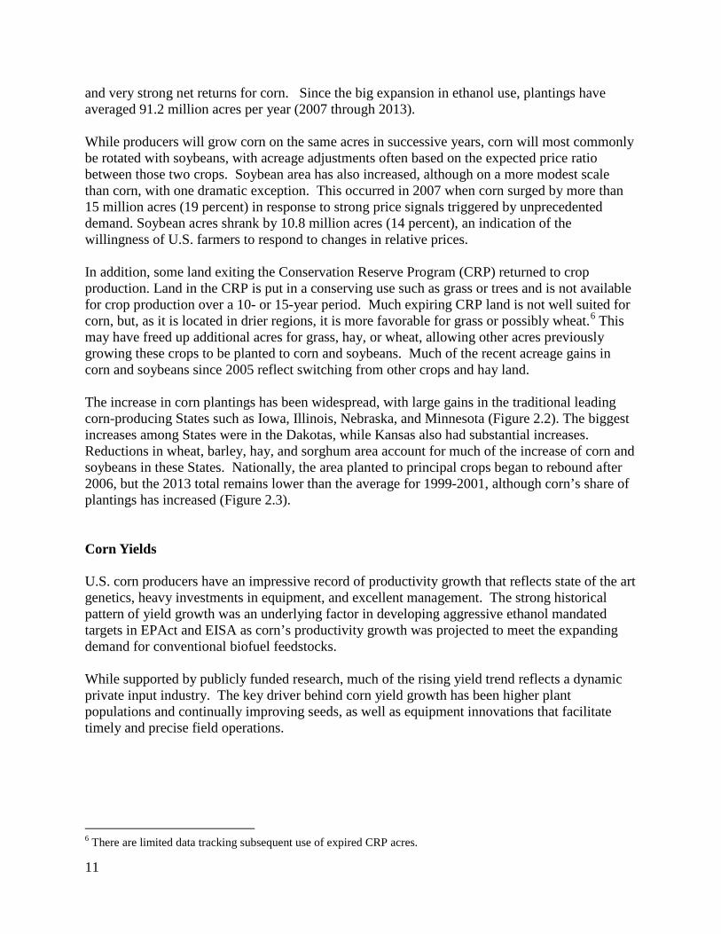
Food, Seed and Industrial Use This category is increasingly dominated by corn used for ethanol (Table 2.3). The other FSI uses have been fairly stable, but shrinking as a share of the total, as the ethanol component has grown. Direct food use of corn is fairly small in the United States and is mostly tracked in the “cereals” sub-category that includes corn used in snacks, breakfast cereals, tortillas, and similar items. However, products included from the other categories of use such as starch and glucose are used in a myriad of beverages and processed foods. Corn bushels that are used to produce various sweeteners have been fairly stable in total. Within this group, however, domestic use of high fructose corn syrup (HFCS) has fallen somewhat, partly in response to consumer changes in tastes and preferences and some switching to sugar or

Table 2.3. Corn, food, seed, and industrial use, 2000/01-2013/14 HFCS Glucose

& dextrose

Starch Ethanol Beverage alcohol

Cereals & other

Seed

Million bushels 2000/01 536 227 250 630 130 185 19 2001/02 542 227 249 707 131 186 20 2002/03 532 231 258 996 131 187 20 2003/04 530 238 273 1,168 132 187 21 2004/05 525 234 282 1,323 133 189 21 2005/06 545 245 275 1,603 135 190 20 2006/07 535 259 277 2,119 136 190 24 2007/08 523 256 265 3,049 135 192 22 2008/09 489 245 234 3,709 134 192 22 2009/10 512 257 250 4,591 134 194 22 2010/11 521 272 258 5,019 135 197 23 2011/12 513 294 254 5,000 137 198 25 2012/13 491 292 249 4,641 140 199 25 2013/14 478 308 219 5,134 140 201 23

Note: HFCS is high fructose corn syrup. other sweeteners. Since 2008, an increase in HFCS exports to Mexico has offset much of the decline in domestic use. Corn used for starch is influenced by food uses and industrial demand in a very wide variety of products such as paper, cardboard, construction, pharmaceuticals, and others, and as such tends to reflect the ups and downs of the general economy. In addition, several research efforts are developing new applications for products derived from corn to replace petroleum-based materials. There have been no major impacts on output in this sector from the rise in ethanol production and higher corn prices. There was a noticeable decrease in exports of corn starch in 2008 and 2009 that likely reflected higher prices.

27

Corn Used for Ethanol Corn used for ethanol has increased steadily, for reasons discussed earlier. In recent years, corn has accounted for about 98 percent of ethanol feedstocks, with grain sorghum a distant second. Corn use for ethanol more than tripled between 2005 and 2010 (Figure 2.15). The share of corn production used to meet ethanol demand has increased from less than 10 percent in 2000 to as high as 43 percent in the 2012 drought year. Figure 2.15. Corn use for ethanol and ethanol share of corn production, 2000/01-2013/14

Corn Trade and Exports The United States has long been the world’s leading corn exporter. However, U.S. corn exports declined since the record high of 2007/08 (Figure 2.16). The recent decline is largely the result of higher prices that made the United States less competitive in world markets and helped to stimulate more corn production in the rest of the world. The export decline also reflected falling corn supplies from 2010/11 on below-trend yields that culminated with the 2012 drought. This led to a major decline in U.S. exports in 2012/13 to the lowest volume since 1971 on both the local marketing year and international trade year. As corn exports declined in recent years, their share of total use and production also shrank to a modern low of under 7 percent by 2012, the lowest since 1959 (Figure 2.17). U.S. exports rebounded sharply in 2013/14 on a big supply increase and lower prices. As with corn feed and residual, it is possible to get a broader picture of total export disappearance by adding distillers’ grains exports to corn exports. Distillers’ grain exports rose sharply in recent years with expansion of ethanol production from dry mills; however, even adding these to corn grain exports, the total declined dramatically until 2013/14 (Figure 2.18.)

0%

5%

10%

15%

20%

25%

30%

35%

40%

45%

50%

0

1

2

3

4

5

6

Ethanol Production and Share of Corn Production

Ethanol

Share corn prod.

Billion bushels

28

Figure 2.16. U.S. corn exports, 2000/01-13/14

Figure 2.17. Export share of U.S. corn production, 2000-13

Along with the decline in U.S. corn exports, the United States also suffered a major loss of world market share in recent years. By 2012/13, the U.S. share of global corn trade had plunged to 18 percent, the worst in modern history (Figure 2.19). Even with the strong gains in 2013/14 export volume, there was only a partial recovery of the U.S. world export market share, which remained below the historical average. Prior to the recent downturn, the U.S. market share, historically averaged over 60 percent. The marked erosion of U.S. exports was not a result of slowing global demand for corn, but instead greater competition from other exporters as corn prices rose to unprecedented highs. World corn trade has been booming, with only a temporary contraction in 2008/09, when a global recession occurred at the same time that commodity prices, including

0.0

0.5

1.0

1.5

2.0

2.5

3.0

U.S. Corn Exports Billion bushels

0%

5%

10%

15%

20%

25%

2000/01 2001/02 2002/03 2003/04 2004/05 2005/06 2006/07 2007/08 2008/09 2009/10 2010/11 2011/12 2012/13 2013/14

Export Share of U.S. Corn Production

29

Figure 2.18. U.S. exports of corn plus distillers’ grains, marketing years 2000-12

* converted to corn bushel equivalent. Figure 2.19. World corn trade and U.S. export share, 2000/01-2013/14

energy, soared. World corn trade set a new record in 2011/12 and then surpassed that record by a large margin in 2013/14. The increase in export competition largely reflects a response to the strong incentives to increase production that were provided by high prices. Over the last decade, corn production outside of the United States has increased by more than U.S. production, despite large U.S. acreage gains (Figure 2.20). The gains in non-U.S. production are a result of both an increase in area and an

0

500

1,000

1,500

2,000

2,500

3,000

U.S. Exports of Corn Plus Distillers' Grains *

Distillers' grains

Corn

Million bushels

0%10%20%30%40%50%60%70%80%

0

20

40

60

80

100

120

140

World Corn Trade and U.S. Export Share

World trade

U.S. share

Million metric tons

30

Figure 2.20. U.S. and foreign corn production, 2000-13

Figure 2.21. Non-U.S. corn area harvested, 2000/01-2013/14

increase in yield. Compared with 2000, foreign corn area harvested rose 35 percent by 2013 (Figure 2.21) and average yields increased 37 percent (Figure 2.22). While the upward trends in foreign area and yield were already evident, the rates of increase accelerated in 2011 as world prices climbed. Very high yields reflected incentives to invest more in inputs, along with generally favorable weather. Many countries could be considered relatively less advanced in production technology. However, simply adopting modern hybrid seed, for example, in place of traditional open-pollinated seed, can lead to sharp yield increases. Similarly, higher fertilizer use, where its use has been limited, typically brings a strong production response.

0

20

40

60

80

100

120

140

160

2000 2001 2002 2003 2004 2005 2006 2007 2008 2009 2010 2011 2012 2013

Non-U.S. Corn Area Harvested Million hectares

0

100

200

300

400

500

600

700

2000 2001 2002 2003 2004 2005 2006 2007 2008 2009 2010 2011 2012 2013

U.S. and Foreign Corn Production

Foreign

U.S.

Million metric tons

31

Figure 2.22. World average, less U.S. corn yields, 2000-2013

The high-price environment contributed to large increases in exports from some countries that traditionally competed with the United States, but it also stimulated exports from some newer players, who were not competitive at lower price levels. Some of the competing exporters, such as Ukraine, were relatively low-cost producers, but they had limited infrastructure for exports, which boosted shipping costs. Some others were relatively high-cost producers who would not normally export large amounts of corn if prices were lower, as was the case for India. In any event, competing exporters have captured most of the recent growth in world trade, accounting for the decline in U.S. exports and market share. The acreage response to high prices by most competing exporters was very pronounced. Aggregate harvested area for seven countries increased by 12 million hectares (nearly 30 million acres) from 2000 to 2013, a 47-percent increase (Figure 2.23).16 The growth in area was accompanied by increases in yields. Over 2000-2013, weighted average yields for this group of countries went up over 50 percent, even with a substantial non-commercial segment in some of the countries (Figure 2.24). The weighted average increase—from 3.2 metric tons per hectare to 5 metric tons—is equivalent to a change from about 50 bushels per acre to 80 bushels. Paraguay and Russia, the smallest corn producers in this group, each doubled yields. Aggregate corn production of the competing exporter group thus increased sharply—up 131 percent between 2000 and 2013, increasing exportable supplies and leading to big gains in export shipments (Tables 2.4 and 2.5). 16 These include Argentina, Brazil, Canada, India, Paraguay, Russia, and Ukraine. Some corn exporting countries did not display a noticeable area change in this period and were not included in the aggregate calculations. These include Serbia and South Africa. Although China and the EU increased corn area, they were excluded since they are currently net importers.

2.0

2.5

3.0

3.5

4.0

4.5

2000 2001 2002 2003 2004 2005 2006 2007 2008 2009 2010 2011 2012 2013

Average Non-U.S. Corn Yields

Metric tons per hectare

32

Figure 2.23. Selected exporters’ corn area for competitors showing strong acreage response, 2000-13

Figure 2.24. Weighted corn yield of selected export competitors, 2000-13

0

5

10

15

20

25

30

35

40

2000 2001 2002 2003 2004 2005 2006 2007 2008 2009 2010 2011 2012 2013

Selected Exporters' Corn Area For Competitors Showing Strong Acreage Response

Ukraine

Russia

Paraguay

India

Canada

Brazil

Argentina

Million hectares

2.0

2.5

3.0

3.5

4.0

4.5

5.0

5.5

2000 2001 2002 2003 2004 2005 2006 2007 2008 2009 2010 2011 2012 2013

Selected Exporters' Weighted Yields For Competitors Showing Strong Acreage Response

Metric tons per hectare

33

Table 2.4. Corn production of other major exporters, 2000-13

Argentina Brazil Canada India Paraguay Russia Ukraine Sum Million metric tons

2000 15.4 41.5 7.0 12.0 0.9 1.5 3.8 82.1 2001 14.7 35.5 8.4 13.2 1.1 0.8 3.6 77.3 2002 15.5 44.5 9.0 11.2 1.1 1.5 4.2 86.9 2003 15.0 42.0 9.6 15.0 0.8 2.0 6.9 91.3 2004 20.5 35.0 8.8 14.2 1.1 3.4 8.9 91.8 2005 15.8 41.7 9.3 14.7 2.0 3.1 7.2 93.8 2006 22.5 51.0 9.0 15.1 2.6 3.5 6.4 110.2 2007 22.0 58.6 11.6 19.0 1.9 3.8 7.4 124.3 2008 15.5 51.0 10.6 19.7 1.8 6.7 11.4 116.8 2009 25.0 56.1 9.8 16.7 3.1 4.0 10.5 125.1 2010 25.2 57.4 12.0 21.7 3.1 3.1 11.9 134.5 2011 21.0 73.0 11.4 21.8 2.0 7.0 22.8 158.9 2012 27.0 81.5 13.1 22.3 3.0 8.2 20.9 176.0 2013 26.0 80.0 14.2 24.3 2.5 11.6 30.9 189.5

Table 2.5. Corn export volumes of other major corn exporters, 2000/01-2013/14

Argentina Brazil Canada India Paraguay Russia Ukraine Sum Other

Non-U.S. Million metric tons 2000/01 12.2 3.7 0.1 0.1 0.5 0.0 0.4 17.1 10.5 2001/02 8.6 3.9 0.2 0.0 0.2 0.0 0.3 13.2 12.2 2002/03 12.3 3.2 0.3 0.1 0.8 0.0 0.8 17.5 18.4 2003/04 10.4 5.8 0.4 1.2 0.6 0.0 1.2 19.7 10.5 2004/05 13.8 1.4 0.2 0.5 0.4 0.0 2.3 18.7 12.0 2005/06 10.7 2.8 0.2 0.5 1.3 0.1 2.5 18.0 8.4 2006/07 15.7 8.1 0.3 0.5 1.9 0.1 1.0 27.5 9.5 2007/08 15.7 7.9 0.9 5.1 1.4 0.0 2.1 33.1 4.4 2008/09 8.5 7.2 0.4 2.6 1.8 1.3 5.5 27.2 8.6 2009/10 17.0 8.6 0.2 1.9 1.4 0.4 5.1 34.6 8.5 2010/11 15.2 11.6 1.7 3.4 1.2 0.0 5.0 38.1 8.5 2011/12 16.5 12.7 0.5 4.7 2.2 2.0 15.2 53.7 11.6 2012/13 22.8 26.0 1.8 4.8 2.9 1.9 12.7 72.9 9.4 2013/14 12.8 22.0 1.9 3.9 2.7 4.2 20.0 67.6 11.9

34

Corn Trade and Imports Corn imports account for a miniscule portion of the U.S. corn supply. Generally, Canada is the main supplier, with small amounts imported from Mexico. However, over 2010/11 to 2013/14, imports increased from an average of 12 million bushels per year to close to 30 million in 2010/11 and 2011/12 (Figure 2.25). Then in 2012/13, in the wake of the drought, imports soared to 160 million bushels. Brazil became the largest supplier, meeting the needs of animal feeders in the U.S Southeast who previously obtained supplies from regions most impacted by the 2012 drought. Corn imports declined to 36 million bushels in the 2013/14 corn marketing year, but were still above the historical average. Corn Prices U.S. corn prices have risen sharply since 2006, in part because of the huge demand spike from ethanol. Average prices received by farmers began to increase in 2006 and hit several record highs since then. Farm prices averaged $2.10 per bushel ($82.80 per metric ton) between 2000 and 2005, and then began to rise in 2006 (Figure 2.26). The average farm price over 2006-2013 was $4.70 per bushel ($185.19 per metric ton). In 2006/07, the first year of rapid expansion in ethanol production, the season-average price of corn jumped 52 percent to $3.04 per bushel. The next year, it rose another 38 percent to $4.20, eclipsing the previous high of $3.24 set in 1995/96. Most of the impetus for this initial price spurt was demand, led mainly by ethanol in the 2006/07 marketing year and, in the following year by strong growth in ethanol, exports, and feed and residual use. Despite continued large Figure 2.25. U.S. corn imports, 2000/01-2013/14

increases in ethanol production from corn, prices moderated in 2008/09 and 2009/10 on supply gains and reductions in other uses. Prices resumed their ascent in 2010/11 as supply problems developed due to poor weather, setting a new record of $5.18 per bushel. Prices peaked in 2012/13 at $6.89 per bushel when severe drought cut yields drastically and slashed corn

020406080

100120140160180

U.S. Corn Imports Million bushels

35

Figure 2.26. Average corn price received by farmers, 2000/01-2013/14

Figure: 2.27. U.S. corn free on board (FOB) Gulf price quotes, 2000/01-2013/14

production by nearly 1.6 billion bushels. Corn used for ethanol and other purposes, including exports and feeding, fell in that year, given very tight corn supplies and record high prices. Historically, the United States has set the world price for corn, as the dominant producer and trader, and changes in the U.S. situation are quickly transmitted to the rest of the world. U.S. export prices for corn shot up with the increase in farm gate prices after 2005 and were further supported due to pressure from strong import demand and record-high fuel costs. Like farm prices, export prices more than doubled in this period (Figure 2.27). Marketing margins, defined here as the difference between the farm price and export price, went up sharply as well, then fell

0.00

1.00

2.00

3.00

4.00

5.00

6.00

7.00

8.00

Average Corn Price Received by Farmers, Sept.-Aug marketing year

Dollars per bushel

0

50

100

150

200

250

300

350

2000/01 2001/02 2002/03 2003/04 2004/05 2005/06 2006/07 2007/08 2008/09 2009/10 2010/112011/12 2012/13 2013/14

U.S. Corn Export Price Quotes FOB Gulf Sept.- Aug. year

Dollars per metric ton

36

back temporarily late in 2008 with the retreat in oil prices and economic recession (Figure 2.28). Export prices also fell in 2009 with the fall in the farm price but then resumed growth and surpassed the 2008 record by 2011. Figure 2.28. FOB Gulf corn price margin over farm price, 2000/01-2013/14

Note: FOB is free on board. Several factors account for the upward price trend for corn that developed from 2006/07, but ethanol was clearly a significant factor in that first year. There was a marked impact on the corn market early in the 2006/07 marketing year as corn use for ethanol production increased. Whereas prices normally fall to a seasonal harvest low in early October, in 2006 the market staged a counter-seasonal rally, also fueled by some slippage in the crop estimates as the harvest progressed. This is illustrated in Figure 2.29, which shows daily cash prices for corn in 2006 contrasted with the previous year. The season-average farm price of corn increased over 50 percent to $3.04 per bushel that year. A decline in supply accounts for part of this price increase, but most of the price gain can be attributed to ethanol. Corn used for ethanol increased by 516 million bushels, feed and residual use fell by 575 million bushels, and other uses of corn were about unchanged. The ratio of ending stocks-to-use, a common price indicator, fell to 11.6 percent (Figure 2.30). This was comparable to that of 2002/03 when the ratio was 11.4 percent, yet the price that year averaged only $2.32 per bushel. Historical price relationships started to become less useful for forecasting and analysis.

0.00

0.20

0.40

0.60

0.80

1.00

1.20

1.40

1.60

1.80

2.00

2000/01 2001/02 2002/03 2003/04 2004/05 2005/06 2006/07 2007/08 2008/09 2009/10 2010/112011/12 2012/13 2013/14

FOB Gulf Price Margin Over Farm Price Sept.-Aug. Year

Dollars per bushel

37

Figure 2.29. Daily cash corn price movements, 2005/06 and 2006/07

Source: Minneapolis Grain Exchange Figure 2.30. Corn ending stocks and stocks-to-use ratio, 2000/01-2013/14

While ethanol remained the major driver of growth in demand for corn in the following years, many other factors began to add to price pressure and complicate the situation. Strong international demand for grains and oilseeds, a widespread commodity boom, and huge inflows of speculative and investor money all helped push corn and other agricultural prices higher. A growing link between energy prices and corn as the ethanol component of the fuel supply increased also exposed corn to more price volatility. Historically, there had been little correlation between corn and oil prices (Figure 2.31).

1.00

1.50

2.00

2.50

3.00

3.50

4.00

4.50

Sept Oct Nov Dec Jan Feb Mar Apr May June July Aug

Daily Cash Corn Prices 2005/06 and 2006/07

2006

2005

Dollars per bushel

0%

5%

10%

15%

20%

25%

0

500

1,000

1,500

2,000

2,500

Corn Ending Stocks and the Stocks-to-Use Ratio

end stocks

s/u ratio

Million bushels

38

Figure 2.31. Corn price versus crude oil price, 1950-2013

The increase in volatility and departure from historical patterns was demonstrated in 2007/08 when the corn price increased another 38 percent to $4.20 per bushel even though supply gains outpaced increased use, leading to an increase in ending stocks (Figures 2.26 and 2.30). The stocks-to-use ratio increased from 11.6 percent to 12.8 percent, which would normally have indicated that prices would decline. In 2008/09, corn prices moderated somewhat, down 3 percent or $0.14 per bushel off the record high of the prior year, and more in line with expectations. Total corn use declined and ending stocks went up slightly, raising the stocks-to- use ratio. End users were battered by the cumulative impact of high prices, volatility, and market uncertainty. The 2008 year was arguably the most turbulent in commodity history, complicating analysis of all influences on the markets. Crude oil peaked at an all-time high of over $140 a barrel in July and then plummeted to under $40 in December. Economic recession, major financial upheavals, and a big drop in global grain trade led to tremendous uncertainty in markets, and there was massive outflow of investor funds from commodities. Corn prices declined in 2009/10 on an increase in supply and further stock building. Corn prices then resumed their upward path in the following 3 years, setting new highs in 2010/11 through 2012/13 on production problems and support from a general recovery in overall commodity markets. Commodities were generally aided by financial stimulus measures, such as low interest rates promoted by the U.S. Federal Reserve and the stimulus provided by heavy Government spending by China, and more investors began to pour money back into these markets (Figure 2.32). Looking back over the period starting in 2000, demand for corn became increasingly dominated by ethanol as most other uses showed some declines in the 2006-2012 period, as shown in Table 2.6. Changes in corn prices also have had large impacts on other grains and oilseeds. Prices for

0.00

1.00

2.00

3.00

4.00

5.00

6.00

7.00

8.00

0

20

40

60

80

100

120

1950

1953

1956

1959

1962

1965

1968

1971

1974

1977

1980

1983

1986

1989

1992

1995

1998

2001

2004

2007

2010

2013

Corn Price versus Crude Oil Price

OIL

CORN

$ per barrel $ per bushel

Oil: Refiner acquisition cost Corn: Farm price

39

other crops tend to move roughly in tandem with corn through cross-price effects, market interactions, and, in many cases, competition for acreage (Figure 2.33). Prices for co-product Figure 2.32. Ethanol expansion and higher corn prices coincided with general commodity boom

Note: IMF is the International Monetary Fund.

Table 2.6. Annual change in the corn balance sheet, 2001/02-2013/14

Marketing year

Supply Ethanol Feed & residual

Exports Other uses

Ending stocks

Farm price

Million bushels $ 2001/02 -228 77 27 -37 8 -303 0.12 2002/03 -834 288 -300 -317 5 -510 0.35 2003/04 610 172 233 312 22 -129 0.10 2004/05 1,586 156 354 -82 3 1,156 -0.36 2005/06 460 280 -20 316 31 -147 -0.06 2006/07 -725 516 -575 -8 6 -664 1.04 2007/08 1,851 930 318 312 -29 321 1.16 2008/09 -681 660 -724 -588 -77 49 -0.14 2009/10 1,068 882 -32 130 54 34 -0.51 2010/11 -588 428 -324 -148 37 -580 1.63 2011/12 -690 -19 -257 -290 14 -139 1.04 2012/13 -1,567 -359 -205 -811 -24 -168 0.67 2013/14 2782 493 719 1187 -28 411 -2.43 Cumulative changes

3,047

4,50

-788

-24

22

-667

0

50

100

150

200

250

2000 2001 2002 2003 2004 2005 2006 2007 2008 2009 2010 2011 2012 2013

Ethanol Expansion and Higher Corn Prices Coincided With General Commodity Boom

IMF Commodity Price Index (includes Fuel and Non-Fuel)

2005=100

40

Figure 2.33. Average farm prices, soybeans, wheat and other feed grains

feeds also rose over this period. While the corn price was a key driver for distillers grain and corn gluten feed prices (Figure 2.34), there was some impact from changes in soybean and soybean meal prices, because of the higher protein content of the co-products. A strong soybean price increase in 2003/04 was mainly due to a short soybean crop. Figure 2.34. Distillers’ dried grains (DDG) and corn gluten feed prices

0.002.004.006.008.00

10.0012.0014.0016.00

Average Farm Prices Soybeans, Wheat, and Other Feed Grains

soybeans

wheat

sorghum

barley

oats

Dollars per bushel

Marketing year basis, varies by crop

0

50

100

150

200

250

300

Distillers' Dried Grains and Corn Gluten Feed Prices

DDG

Corn gluten

Dollars per short ton

Sept.-Aug. average

41

Chapter 3: Managing the U.S. Corn Transportation and Storage System Marina Denicoff Peter Riley

America’s agricultural producers depend on transportation as the critical link between their farms and their customers, both here and abroad. Transportation demand is frequently referred to as a derived demand because the production and consumption of an agricultural commodity create the demand for transportation services. As such, it is an essential part of marketing—any change in supply or demand of the underlying commodity can affect the transport system’s efficiency by bringing about either shortages or surpluses in transportation capacity. Short-term agricultural transportation demand is influenced by variation in annual crop size and location, the timing of planting and harvesting, weather-related transportation disruptions, global trade patterns, crop quality concerns, and commodity price fluctuations. These and other factors can translate into unexpected shifts in transportation patterns and costs, adding to the ever-present commodity price risk to be managed by agricultural producers, processors, and shippers. Corn is shipped by rail, barge, and truck to feedlots, feed mills, other processors, ethanol refineries, and ports for export (Figure 3.1). Corn exporters mostly depend on rail and barge services to move the crop to ports; domestic corn movements are primarily handled by trucks. Consequently, volatility in the corn export market creates an element of uncertainty in anticipating the demand for transportation services. The U.S. corn marketing year begins on September 1 when the fall harvest gets underway, and it ends the following year on August 31. The futures markets developed over time to establish a price discovery mechanism so that producers could make planting decisions and consumers could plan for allocation of the crop. Market carry and basis (discussed below) provide market price signals to help grain producers and shippers make their grain storage and marketing decisions. Those decisions subsequently have transportation demand implications, making market carry an indicator of derived transportation demand. Market carry—or carrying charge—is the price difference between the future delivery month and the near-term month (e.g., December and March corn futures, or January and March soybean futures); it represents how much the market is offering the producers to hold (carry) the grain until the distant month.1 Basis is the amount by which the cash price in a given location differs from the nearby futures contract price, which changes daily. Analysis of basis and market carry can provide an estimate of what the market might be paying for storage, encouraging sellers either to hold on to the grain or to deliver it to the market. To market their grain, some farmers use forward contracting and, in recent years, basis contracting to manage their price risk.2 Along with the development of the agricultural commodity futures markets and grain producing and

1 Carrying charges, cost of carry, and full carry are used interchangeably. The basic definition of carry is the cost of storage

space, insurance, and finance charges incurred when storing a physical commodity. The actual costs may vary by location based on differences in interest, storage and insurance rates.

2 Source: Carry and Basis: Grain Market Signals and Transportation Implications, USDA Agricultural Marketing Service, Grain Transportation Report, December 23, 2010, pp. 2-3

42

Figure 3.1. Corn production, ethanol plants, export ports, and the transportation system

*GCAU is grain-consuming animal units. Sources: USDA, Agricultural Marketing Service analysis of the USDA, National Agricultural Statistics Service county-level statistics 2013, and USDA, Federal Grain Inspection Service port inspection data, 2013: http://www.ams.usda.gov/AMSv1.0/getfile?dDocName=STELPRDC5108805. Also see Denicoff et al, 2014. processing industry, a vast network of storage facilities with access to rail, barge, and truck transportation developed in the producing regions (Figure 3.2). The map in Figure 3.2 includes storage operations that warehouse several commodity groups. Each warehouse may hold different commodities at different times of the year or, in multi-silo elevators, different commodities at the same time. However, the vast majority of elevators primarily handle grains.

43

Figure 3.2. Location of elevator storage capacity, with rail and barge systems

Source: USDA, Farm Services Agency USWA/UGRSA database (as of January 2009). This database is estimated to include more than 80 percent of total storage capacity. Corn Storage The option to store grain is a key component of marketing for producers. Similarly, storage is a critical tool for end users. In each case, the use of storage enables the seller or buyer to take advantage of temporal changes in prices and markets. The corn market typically has a seasonal low at harvest time when there is a high concentration of sales and the largest available supply of the year. This is also the best time for end-users to buy. Storage facilitates consumer buying at a favorable time, with the grain stored for future use. Farmers also have an interest in storing corn and selling later in the year as prices rise. As previously discussed, the “carry” in the market varies and provides signals to both producers and users to help guide storage decisions. In recent years, there has been considerable growth in both on-farm and off-farm storage (Figure 3.3). In 2013, on-farm capacity was estimated at 13 billion bushels, accounting for 56 percent of the total capacity of 23.4 billion bushels. Among grains, corn accounts for the largest use of this capacity. Despite the recent expansion, there was considerably more storage available in the 1980s when Government policy supported large stock holding, including a farmer-owned reserve. Policies have changed dramatically since then, discouraging Government stock procurement. One of the major incentives for the recent expansion in on-farm storage has been the growth of the ethanol industry and its model that generally minimizes storage at individual plants. Instead, the industry mostly follows a “just-in-time” delivery system whereby farmers deliver grain year- around to the plants that are located throughout major corn-producing regions. The plants themselves have only enough storage to maintain a pipeline for fairly immediate operations, minimizing their capital requirements.

44

Figure 3.3. U.S. grain storage capacity, 2000-2013

Source: USDA, Total Grain Storage. Transportation of Corn by Mode Between 2007 and 2011, corn accounted for approximately 65 percent of all grains moved in the United States (USDA, Agricultural Marketing Service, 2012). Between 2007 and 2011, trucks moved, on average, 76 percent of domestically used corn, peaking at 81 percent in 2010 as U.S. exports, as a share of production, declined. Rail transportation averaged 23 percent of domestic corn movement, decreasing from 26 percent in 2007 to 20 percent in 2011. Barge share of the domestic corn movements remained unchanged at 1 percent. The relative increase in the amount of corn transported by truck reflects the increase in ethanol production. Most ethanol plants are located within 50 miles of corn-producing areas, and trucks are highly efficient for short-distance transportation. They are usually more efficient than rail for destinations within about 250 miles (USDA, Agricultural Marketing Service, 2010). Most corn destined for exports is transported to major ports in the Gulf or Pacific Northwest by barge and/or rail. From 2007 to 2011, barges moved an average of 53 percent of export-bound corn and rail moved 38 percent. Trucks accounted for only 9 percent of transport to export points because most growing areas are far from ports or export destinations and barge or rail transportation is more efficient over large distances.

0

5

10

15

20

25

2000 2001 2002 2003 2004 2005 2006 2007 2008 2009 2010 2011 2012 2013

U.S. Grain Storage Capacity

Off-farm

On-farm

Billion bushels

45

Chapter 4: Corn Ethanol Processing Technology, Cost of Production, and Profitability Paul Gallagher The typical corn ethanol processing facility is a dry mill. Dry mills grind dry corn to produce ethanol and a composite coproduct called distillers’ grains, which consists of the residual corn components after starch is removed for ethanol production. The size of dry mills constructed during the last 15 years has increased from about 15 million gallons per year (MGY) to 40-100 MGY. The baseline processing plant in this section uses natural gas for distillation and drying distillers' grains, and purchased electricity powers the plant. A plant that dries distillers' grains can move the product by truck, rail, barge, or ship to international markets. Distillers' grains can also be fed “wet” to livestock, but distribution is limited by transportation costs. The estimated costs of production for a typical plant in May 2015 are shown in Table 4.1. A total of $1.30 per gallon was sufficient to recover total production costs.

Table 4.1. Ethanol production cost with major components, May 2015 basis, dollars/gallon

Net corn cost 0.703 Cash operating costs: 0.375 Natural gas 0.165 Electricity 0.041 Non-energy1 0.169 Annualized capital cost2 0.220 Total cost 1.298

1Includes materials, maintenance, labor, and administrative costs. 2The annual payment required for paying a 15-year mortgage at 11 percent interest and a plant capital cost of $1.58 per gallon of capacity. A time series of ethanol cost components is shown in Figure 4.1. Most of the annual variation in total costs is attributable to net corn costs (corn cost minus coproduct revenue), especially the cost escalation that began in 2006. Other costs have declined slightly, from $0.62 per gallon in 1990 to $0.60 per gallon in 2015, despite nearly three decades of general inflation throughout the U.S. economy. A $0.35/gallon estimate approximates the cost-reducing benefits from increases in automation, labor efficiency, energy savings, enzyme improvements, and economies of scale (Gallagher et al., 2007). From 1994 to about 2006, total production cost ranged between $1.00 and $1.25 per gallon. Since then, production costs drifted upwards, reflecting mainly increasing net corn costs.

46

Data for the ethanol costs series combine surveys and engineering cost estimates. Three surveys give benchmarks for input use, operating cost, and plant construction cost during the 1987-2008 period (Shapouri et al 2000, Shapouri and Gallagher, 2005; Shapouri et al 2010). Survey benchmarks are then adjusted for changing input energy prices and financial market conditions. From 2013, cost estimates for non-energy operating costs and capital costs are taken from an engineering cost estimate (McAloon). The engineering cost estimate, calculated in July, is $0.13 per gallon less than the estimate for July 2013 given in figure 4.1—the differences are reconciled entirely by net corn costs ($0.10/gallon) and plant capital costs ($0.03/gallon) due to a higher investment risk premium. There are several modifications of the basic ethanol plant configuration that can improve energy balance, enhance the global warming profile, or reduce costs if they fit the plants’ situation. First, ethanol processing plants that are 30 miles or less from a cattle population can transport the distillers' grains wet and save substantial corn drying costs. According to a recent survey, drying distillers' grains requires 12,936 British thermal units (Btu) per gallon of natural gas and 0.155 kilowatt hours (kWh)/gallon of electricity (Shapouri and Gallagher). So the cost of a gallon of ethanol could be reduced by $0.066/gal if the distillers' grains are not dried. A comparison of costs and returns for drying distillers' grains, based on recent Iowa prices, suggests that net revenue is higher without drying, but wet distiller grains are sold at a discount, so not drying results in a net saving of $0.041/gallon.

0.00

0.50

1.00

1.50

2.00

2.50

3.00

Dollars per gallon

Year/Month

Figure 4.1. Ethanol cost of production, 1/1990 to 1/2015

Total Cost Net corn cost Other cost

47

Second, most plants today are also offsetting costs by installing equipment to remove the corn oil fraction from the dry distillers' grains, and then using the low-grade corn oil to heat the ethanol plant or sell it as feedstock for biodiesel production. Estimates suggest that a cost reduction of $0.04/gallon can be achieved with the quick-germ process. Third, many firms arrange to buy new high-starch corn varieties that can increase ethanol yield above the industry average. Estimates suggest that processor cost can be reduced by $0.13/gallon as ethanol yields increase and yields of dry distillers' grains decrease, but those advantages could be offset by increased seed costs (Gallagher, 2009, p. 25). Fourth, some firms are using biomass power to improve energy balance and their global warming profile (Gallagher and Shapouri, 2009). Processing Margins and Profitability The ethanol processing margin defines a composite market price for processing one unit of corn. It consists of ethanol and distillers' grains revenues per unit of corn processed, less the corn input price. Margins should, under most conditions, signal an expansion of production when they are high and a contraction of production when low. When compared to non-corn operating costs and plant capital costs, the processing margin provides a good summary measure of ethanol plant operating economics (Gallagher et al., 2007). Plant closure is indicated when the gross margin falls below variable operating costs. Plant capacity expansion is a possibility when the processing margin exceeds the sum of variable operating costs and the annual payment on a mortgage for the capital purchase of one unit of capacity and is expected to remain favorable over a period to repay debt. In fact, regressions between processing capacity and processing margin are statistically significant (Gallagher and Shapouri, 2009). Figure 4.2 shows the margins and cost estimates, marking the main profitability and loss episodes in the ethanol industry since 1990. Margins are ethanol revenues plus dry distillers' grains revenues less corn costs. Margins were mostly positive in the early 1990s, but starting in the mid-1990s, there was a 3-year period when many plants shut down, or operated at a level just covering cash operating costs. This period coincides with petroleum prices of $15 per barrel. Margins remained low during most of 1998 and 1999. The effects from the beleaguered methyl tertiary butyl ether (MTBE) market began to have a positive influence on ethanol margins in 2000. There was a 2-year period of strong margins that were considerably above total costs, signaling capacity expansion. The strong margins occurred as MTBE was losing market share to ethanol, effectively doubling ethanol’s market in meeting the oxygen demand for reformulated gasoline (Gallagher, et al., 2003). Capacity expanded and margins fell back to the point where fixed and variable costs were just covered by 2002—there was no investment signal during the 2002-2004 period. The next major move occurred in the 2004-2006 period when exceptionally strong margins indicated a capital payback period of only 1-3 years, likely due to escalating petroleum fuel and ethanol prices and the renewable fuel standard that initially increased ethanol demand beyond fixed processing capacity. After processing capacity began expanding to meet growing ethanol demand during the 2008-12 period, processing margins fell back to earlier levels, moderately above total costs. The margin decline was likely caused by expanding demand for corn ethanol

48

and increasing corn prices. Throughout most of 2013, corn prices remained high due to the combined effects of drought and a steadily expanding RFS, squeezing the profitability out of continued high ethanol prices. However, with a record harvest for the 2013 corn crop and the leveling off the RFS volume requirements for corn ethanol, corn prices began to drop in the fall of 2013. Another record corn crop in 2014 continued to put downward pressure on corn prices, further reducing corn costs for ethanol producers. Margins improved to the $2/bu to $3/bu range during 2014 and the beginning of 2015.

0

1

2

3

4

5

6

7

8

9

10

$/Bu of corn

Year/Month

Margin Operating+capital costs Cash operating costs

Figure 4.2. Corn processing margin and costs for dry mills, 1/1990 thru 5/2015

49

Chapter 5: Ethanol Distribution, Trade Flows, and Shipping Costs

Paul Gallagher Marina Denicoff Introduction

The distribution system for U.S. transportation fuels evolved over many decades. The infrastructure and equipment were originally developed for liquid petroleum fuels, and ethanol was integrated into the system as it became an important component of gasoline. Petroleum fuels are distributed from the major refining areas in the U.S. Gulf Coast, and to a lesser extent, from western and eastern ports to consumer markets. Since oil refineries are not evenly distributed throughout the United States, the industry has developed a sophisticated transportation network to deliver its products nationwide and also meet the demand of high- consumption areas with dense populations, such as the East Coast, the West Coast, and along the Gulf Coast. Petroleum fuels are generally transported long distances by pipeline, ship, and barge to fuel terminals. When gasoline arrives at a terminal, it usually is blended with up to 10 percent ethanol to make E10. Trucks are then used to move the finished fuel to local retail gas stations or other end-use locations. Ethanol plants are located throughout the country; however, ethanol capacity is concentrated in the Corn Belt—mostly west of the Mississippi River (Figure 5.1). Ethanol transport relies primarily on rail and trucks, and a small amount of Midwest ethanol is moved on barges. The geographical distribution of ethanol consumption is similar to gasoline, since it is usually blended with gasoline to produce E10. The renewable fuel requirement has made E10 the most Figure 5.1. Petroleum Administration for Defense Districts (PADDs)

Source: U.S. Energy Information Administration, 2012.

PADD 4

PADD 5

PADD 3

PADD 2

PADD 1

50

common fuel in the United States. Ethanol is typically delivered by rail to petroleum storage hubs or terminals for blending and/or storage. Trucks are then used to deliver the finished blended fuel to retailers. The rapid growth experienced by the ethanol industry in recent years has caused its transportation network to expand significantly. The remainder of this chapter will describe the transportation infrastructure and technology that has developed to facilitate the increased transportation needs of ethanol. An examination of the ethanol transportation system shows that it is similar to those used to transport large-scale agricultural commodities. Furthermore, it is reasonably efficient and cost competitive. Ethanol Distribution and Trade Flows Economic and policy factors likely determined the location of ethanol production in the corn production area of the United States and consumption in the populated coastal areas. On one hand, production costs are reduced using the cheapest corn in the most remote areas of the Corn Belt. Processing near the raw material saves on shipping costs, since on a gallon basis, ethanol weighs far less than corn (e.g., a 56 pound bushel of corn yields about 20 pounds of ethanol). On the other hand, fuel consumption is concentrated in the more densely populated coastal areas. A few plants located outside of the Corn Belt, so-called destination plants, face more involved logistics, and corn transport increases variable costs. As stated earlier, U.S. ethanol production is concentrated in the Midwestern Corn Belt, while consumption is concentrated in the populated Coastal areas of the East, West, and South. Domestic ethanol trade flows can be examined using data from five "Petroleum Administration for Defense Districts" or PADDs, which provide data on regional fuel movements (Figure 5.1). The Midwest (PADD 2) produced 12.3 billion gallons of ethanol in 2012 and only consumed 28 percent of its production. About one-half (4.3 billion gallons) of PADD 2 out-of-State shipments went to the East Coast (PADD1). Otherwise, Midwestern shipments were evenly split between the West Coast (PADD 5) with 2.0 billion gallons, and the Gulf Coast (PADD 3) with 2.0 billion gallons. About 10 percent of ethanol production is located in the consuming areas. For more details on domestic trade flows see Appendix Figure 1. Foreign trade was not much of a factor in 2012. About 4.7 percent of U.S. production was exported, 0.36 billion gallons from the Gulf Coast and 0.28 billion gallons from the Midwest. Regarding imports, the East Coast acquired 0.38 billion gallons and the West Coast brought in 0.1 billion gallons, together accounting for 3.8 percent of U.S. ethanol consumption. Most imports are Brazilian sugarcane ethanol, which qualifies as an advanced biofuel under the RFS program and California's low carbon fuel standard (see Chapter 1).

51

Figure 5.2. Location of petroleum product terminals capable of blending ethanol

Ethanol is transported by truck, train, or barge from production points to petroleum blending terminals equipped to store and/or blend ethanol (Figure 5.2). Rail and truck are the main modes of ethanol transport, with some locations capable of receiving barges and tanker vessels. Trucks are competitive for relatively short hauls of ethanol, 125 miles or less (Gallagher et al., 2000). Trucks also transport blended fuel to retail gas stations. But rail is the dominant mode for transporting ethanol from the Midwest to Coastal areas-rail accounts for approximately 70–75 percent of ethanol shipments.

History

Shortly after the time the ethanol expansion began in 2005-2006, there were public concerns over the transportation infrastructure regarding shipments from Midwest to Coastal areas (Denicoff, et al.). There was concern that the mandated large volumes of ethanol would strain the rail transportation network. A publicly funded investigation of building a dedicated ethanol

Number of Terminals Per ZIP Code

1 2-4

5+ Main Railroads

Waterways

Source: USDA Agricultural Marketing Service Analysis of Oil Price Information Service/STALSBY Petroleum Terminal, 25th edition.

52

pipeline from the Midwest to the major consumption area on the east coast was mandated by the 2007 Energy Act (U.S. Department of Energy, 2010). A dedicated pipeline was preferable for ethanol because it has different fuel properties than petroleum fuels and, with the exception of a short-distance pipeline in Florida, the two fuels are not shipped in the same pipelines. Nevertheless, a dedicated long-distance pipeline was not recommended because the break-even transport rate estimate of $0.29/gallon at 2.88 billion gallons of annual throughput was considered too high to be competitive. The rapidly expanding ethanol industry went through a period of transportation-related infrastructure adjustments during 2006-2008. These adjustments included a large backlog of new rail tank car orders, expansion of petroleum blending terminals, development of unit train destinations, and construction of hubs for ethanol storage. The railroads generally welcomed the new freight business and, with the exception of a few bottlenecks (at times, railroads had to establish embargoes on ethanol trains due to congestion at destinations), were able to accommodate the expansion in interregional trade. The railroad capacity for shipping ethanol from the Midwest to U.S. Coastal areas was already in place from the grain export expansion of earlier decades; and the grain export market and other freight movements were stagnant during this period. The new large bio-refineries also invested in unit or shuttle-train capacity, another technology widely used in the grain trade. They are long trains with identical cars that carry a single commodity directly from origin to destination. Unit trains are the most efficient way for railroads to transport ethanol. They avoid gathering and switching delays, can be more easily “slotted” onto a railroad’s network, and result in quicker “turns” (i.e., cars loaded, shipped, unloaded, and returned for another load). Unit trains can be used by smaller ethanol producers, but they may need to store product until enough ethanol is ready to fill a train, or multiple producers may share a train. Ethanol became a small but rapidly growing commodity for railroads. Record-setting ethanol production in 2011 coincided with the peak of movements of ethanol by rail. In 2011, railroads terminated over 340,000 carloads (10 billion gallons) of ethanol, up from just 40,000 carloads in 2000 and 43,000 in 2001. By 2012, the most recent year for which data are available, ethanol accounted for 1.0 percent of total rail carloads (up from 0.21 percent in 2003), 1.5 percent of rail tonnage (up from 0.3 percent in 2003), and 2.0 percent of rail ton-miles (up from 0.4 percent in 2003).1 Although ethanol is a small percentage of the overall rail ton-miles, the majority of the shipments travel along several main corridors that at times may experience congestion. Railroad capacity has not been a huge issue for ethanol shippers in the recent years, but competition for rail service has been rapidly rising from the gas production boom in the Bakken formation of Montana and North Dakota.2

1 Association of American Railroads, Policy and Economics Department, “Railroads and Ethanol”, May 2014. 2 Surface Transportation Board, RETAC meeting, EIA Presentation, September 20, 2012

53

Evaluation3

The following analysis examines the impact of transportation costs on ethanol profit margins, since the ethanol producer typically pays for the transportation costs. Consider the freight rates for major rail transportation routes given in Table 5.1. The east-bound routes originate in Chicago and end in three major consumption centers: New York, New Orleans, and Tampa. The eastward rates are calculated from public rates given by CSX, a major railroad corporation. Specifically, a rate-distance function was estimated from 490 rates given for various routes in the Eastern United States. The rail cost estimate is a regression estimate for that distance, which is, in effect, the average of the many rates in the sample near that distance. A rate-distance regression model was defined with the CSX ethanol transport rate as the dependent variable, expressed in $/gallon/mile, and the independent variable was distance, expressed in miles. The exponent of the non-linear freight-distance function was varied in order to obtain the Table 5.1. Rail freight rates by distance and gasoline pipeline margins for various locations, 2013 From: To: Distance Cost Gasoline Margins

Miles

Dollar per

gallon

Dollar per

gallon

27-May 19-Aug Ave.

Chicago, IL New York, NY 790 0.128 0.122 0.225 0.174 Chicago, IL New Orleans, LA 926 0.140 0.157 -0.009 0.074 Chicago, IL Tampa, FL 1,172 0.164 0.235 0.157 0.196

Fairmont, NE

Houston (Deer Park), TX 834 0.143 0.142 0.173 0.158

Fairmont, NE Los Angeles, CA 1,464 0.189 0.245 0.318 0.282 Fairmont, NE Seattle, WA 1,642 0.237 0.163 0.210 0.187

best fit (Figure 5.3). The cost per mile charge implied by these rates flattens to about 1.4 cents per 100 mile at distances of 1,200 miles or greater. The westward rate estimates originate at Fairmont, Nebraska, a major westward and southward shipping point in the ethanol industry. Rates for the main destinations are in the South (Houston) and West (Los Angeles and Seattle). These rates were obtained in a consultation with a representative from a major railroad that operates in the Midwest, South, and West. The rate estimates in Table 5.1 range from $0.128 per gallon of ethanol for Chicago to New York to $0.237 per gallon from Fairmont to Seattle. From discussions with railroad management, it was determined that unit trains of ethanol are uncommon in the Fairmont-to-Seattle route, and Seattle may actually source ethanol more often from Eastern North Dakota. 3 Paul Gallagher is solely responsible for the modeling and rate estimates presented in this section.

54

Figure 5.3. Rail rate ($/gallon/mile) versus distance (miles), actual and regression estimate

* Regression equation: Cd = 0.00009823 +0.08978 d-1.0875 where Cd is the freight rate and d is distance. Adj-R2=0.95 When examining the rail costs for ethanol in Table 5.1, they are generally about the same size as the ethanol price margin snapshot taken in May of 2012. In particular, costs are about equal to the price spread for Houston ($0.142 vs $0.158), Tampa ($0.164 vs $0.196), and Seattle ($0.237 vs $0.187). But costs are somewhat lower than spreads for New York ($0.128 vs $0.174), and Los Angeles ($0.189 vs $0.282). A complete rate-cost analysis would also consider back-hauls, contract rates, fuel surcharges, and destination terminal conditions. But the predictions of the rate-distance regression for actual rates to Houston, Seattle, and LA in table 5.1 are only slightly lower, 6.2 percent on average. Also, a more recent history of price spreads could be helpful. Overall, these rates and costs seem consistent with competitive arbitrage between the source and destination markets on railroads. Comparisons between ethanol shipment costs by rail versus wholesale gasoline margins between the Midwest and the Gulf Coast also provide a rough idea of the competitiveness of a rail transport system for ethanol. First, the ethanol rail rate from Fairmont to Houston is $0.143 per gallon. Compare this to the difference between wholesale prices of regular gasoline in Iowa and on the U.S. Gulf (Figure 5.4). This margin reflects the cost of pipeline shipment in a competitive market. A gasoline pipeline margin of $0.10 per gallon was typical during the 2003-2009 period. However, the gasoline pipeline margin has become more variable and the average has increased to about $0.15 per gallon during the last 2 years. The ethanol freight rate and marketing margin for the Freemont to Houston route compares very favorably with marketing margins for gasoline moving in the opposite direction between similar locations. Second, in comparison to the pipeline study mentioned above, the Chicago-New York ethanol freight rate is less than one-half of the breakeven rate for a pipeline, underscoring the competitiveness of the rail system.

0.000000

0.000100

0.000200

0.000300

0.000400

0.000500

0 200 400 600 800 1000 1200 1400 1600

55

Figure 5.4. Gulf-Iowa wholesale gasoline price margin, 1/1995 -1/2013

Conclusions Transportation is typically the third-highest expense to an ethanol producer—after feedstock and energy. Balancing transportation operating expenses with fixed infrastructure costs can be critical to sustained profitability for each ethanol plant. The rail transport system that has emerged after a decade appears to be performing well. Our evaluation suggests that ethanol rail rates are generally near costs. Furthermore, the rail freight charges for ethanol compare favorably to pipeline rates. So pipeline transportation of ethanol does not seem to be an urgent matter. Still, PADD 2-to-PADD 1 ethanol shipments of 4.3 billion gallons (BGYs) shown in Appendix Figure 1, clearly exceed the 2.9 BGY feasibility threshold mentioned earlier, suggesting another look at the feasibility of an ethanol pipeline.

-0.300

-0.200

-0.100

0.000

0.100

0.200

0.300

0.400

0.500

1995.00 2000.00 2005.00 2010.00

$/ga

l

Year/month

56

Chapter 6: Demand for Ethanol Blending

Anthony Radich1

The United States has been blending ethanol into gasoline since the late 1970s, but only in the last decade or so has ethanol become a significant portion of the gasoline pool. Ethanol was a little over 1 percent of gasoline volume in 2001, but reached nearly 10 percent of domestic gasoline consumption in 2011. The Energy Information Administration measures ethanol utilization by refiners and blenders of gasoline. Figure 6.1 shows a pattern of slow growth in the 1990s, rapid growth in the 2000s, and market saturation and slow growth since 2010. Ethanol began as a regional phenomenon in the Midwest, where most of the corn is grown, but then spread nationwide due to favorable economics, including Federal tax credits worth up to 54 cents per gallon, and the need to replace methyl tertiary butyl ether (MTBE) as a means to add oxygen to gasoline. Gasoline refiners and blenders use ethanol primarily for three different reasons: add to gasoline volume, improve octane, and comply with the RFS mandates. Volume addition was the first application for ethanol when it was reintroduced to the liquid fuels pool in the 1970s. Gasoline refiners and blenders were allowed to add up to 10 percent ethanol to gasoline that was already finished, that is, ready for use by motorists. No change to the gasoline formulation would need Figure 6.1. Refiner and blender net input of ethanol, 1993-2014

Source: U.S. Energy Information Administration Petroleum Navigator. http://www.eia.gov/dnav/pet/hist/LeafHandler.ashx?n=PET&s=MFERIUS1&f=A

1 The analysis and conclusions expressed here are those of the author and not necessarily those of the U.S. Energy Information Administration.

Million gallons

0

2,000

4,000

6,000

8,000

10,000

12,000

14,000

1993 1995 1997 1999 2001 2003 2005 2007 2009 2011 2013

57

to be made at the petroleum refinery. Gasoline would leave the refinery in finished form, and a blender could add ethanol or not depending on whether there was an economic incentive to do so. This practice is known as “splash blending.”

One potential barrier to the addition of ethanol to gasoline was the summer limit on gasoline volatility. Gasoline volatility is measured by a property called Reid Vapor Pressure (RVP), expressed in pounds per square inch (psi). Under the Clean Air Act, all gasoline sold in the summer months must have RVP no higher than 9 psi. The blending of 9-pound gasoline with 10 percent ethanol increases the RVP of the final blend to approximately 10 psi. To facilitate ethanol blending, a waiver allowed ethanol-blended gasoline to exceed the applicable standard by 1 psi. The environmental logic behind the 1-pound waiver was that the increased evaporative emissions from vehicle fuel systems would be offset by decreased tailpipe emissions of carbon monoxide and unburned hydrocarbons. The addition of 10 percent ethanol to gasoline also increases the pump octane rating of the gasoline by over two points. Thus, 87-octane regular gasoline with the addition of 10 percent ethanol would become 89-octane gasoline that could be sold as regular or midgrade gasoline. As ethanol became more widely available, refiners began to plan for its use. They began to produce less finished gasoline and more unfinished gasoline specifically formulated to be blended with ethanol. The unfinished gasoline was both lower in octane and produced in smaller volumes, with the knowledge that ethanol would make up the needed volume and bring the octane up to specification. There are three main varieties of this particular unfinished gasoline: conventional blendstock for oxygenate blending (CBOB), reformulated blendstock for oxygenate blending (RBOB), and California reformulated blendstock for oxygenate blending (CARBOB). A regular-grade blendstock for oxygenate blending has an octane rating of about 84. The use of ethanol in this manner is known as “match blending.” The expansion of ethanol production caused the majority of finished gasoline production to shift from petroleum refiners to gasoline blenders. There are two main reasons for this. Petroleum products, including finished gasoline and blendstocks, are normally transported from the refinery by pipeline. Ethanol can separate out of gasoline or otherwise become contaminated if it comes into contact with the water that is often present in petroleum product pipelines. The result is that the ethanol is moved separately to a petroleum product rack, where tanker trucks are loaded to deliver gasoline and other fuels to service stations or directly to the end customer. Ethanol blending takes place as the gasoline is being loaded onto the truck. The other reason is simple geography. Nearly all of the ethanol production capacity is located in the Midwest, but most petroleum refinery capacity is located along the coasts. The U.S. petroleum product pipeline system is designed to move products from the Gulf Coast, the single largest petroleum-refining region, to consumers in other places. The trend of declining finished gasoline production at the refinery and increasing gasoline production by blenders was well underway when the Energy Information Administration started reporting blender production of gasoline in 2005 (Figure 6.2). In 2005, refiner production of finished gasoline was more than twice the level of blender production. By 2012, that ratio had flipped to where blenders produced 2.6 times the volume of finished gasoline as refiners. The refiners who are still able to produce significant quantities of finished gasoline must have a product rack at or near the refinery to enable the use of ethanol.

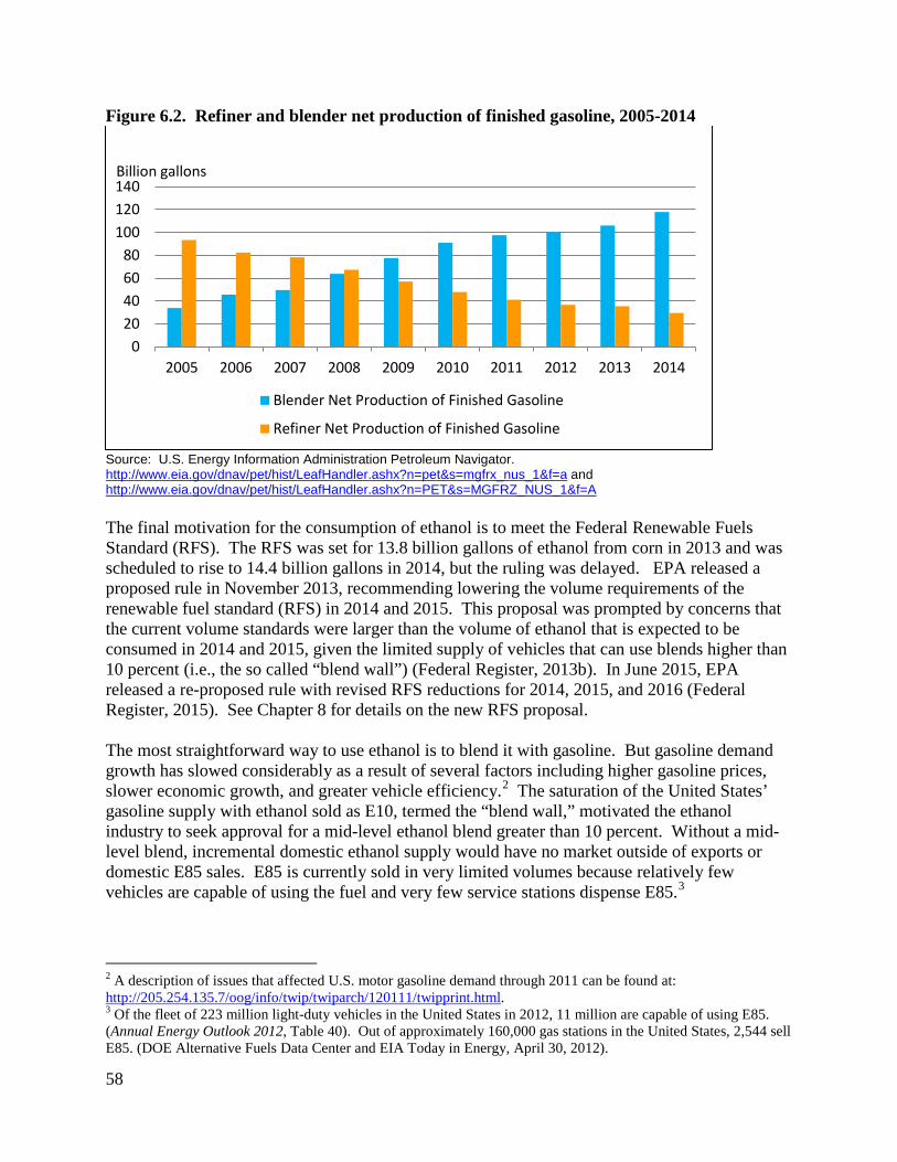
58

Figure 6.2. Refiner and blender net production of finished gasoline, 2005-2014

Source: U.S. Energy Information Administration Petroleum Navigator. http://www.eia.gov/dnav/pet/hist/LeafHandler.ashx?n=pet&s=mgfrx_nus_1&f=a and http://www.eia.gov/dnav/pet/hist/LeafHandler.ashx?n=PET&s=MGFRZ_NUS_1&f=A The final motivation for the consumption of ethanol is to meet the Federal Renewable Fuels Standard (RFS). The RFS was set for 13.8 billion gallons of ethanol from corn in 2013 and was scheduled to rise to 14.4 billion gallons in 2014, but the ruling was delayed. EPA released a proposed rule in November 2013, recommending lowering the volume requirements of the renewable fuel standard (RFS) in 2014 and 2015. This proposal was prompted by concerns that the current volume standards were larger than the volume of ethanol that is expected to be consumed in 2014 and 2015, given the limited supply of vehicles that can use blends higher than 10 percent (i.e., the so called “blend wall”) (Federal Register, 2013b). In June 2015, EPA released a re-proposed rule with revised RFS reductions for 2014, 2015, and 2016 (Federal Register, 2015). See Chapter 8 for details on the new RFS proposal. The most straightforward way to use ethanol is to blend it with gasoline. But gasoline demand growth has slowed considerably as a result of several factors including higher gasoline prices, slower economic growth, and greater vehicle efficiency.2 The saturation of the United States’ gasoline supply with ethanol sold as E10, termed the “blend wall,” motivated the ethanol industry to seek approval for a mid-level ethanol blend greater than 10 percent. Without a mid-level blend, incremental domestic ethanol supply would have no market outside of exports or domestic E85 sales. E85 is currently sold in very limited volumes because relatively few vehicles are capable of using the fuel and very few service stations dispense E85.3

2 A description of issues that affected U.S. motor gasoline demand through 2011 can be found at: http://205.254.135.7/oog/info/twip/twiparch/120111/twipprint.html. 3 Of the fleet of 223 million light-duty vehicles in the United States in 2012, 11 million are capable of using E85. (Annual Energy Outlook 2012, Table 40). Out of approximately 160,000 gas stations in the United States, 2,544 sell E85. (DOE Alternative Fuels Data Center and EIA Today in Energy, April 30, 2012).

020406080

100120140

2005 2006 2007 2008 2009 2010 2011 2012 2013 2014

Blender Net Production of Finished Gasoline

Refiner Net Production of Finished Gasoline

Billion gallons

59

In March 2009, Growth Energy, an ethanol trade organization, and a number of ethanol producers petitioned EPA to approve the use of up to 15 percent ethanol by volume in finished gasoline (E15). In October 2010, EPA approved the use of E15 in vehicles of model year 2007 or newer after conducting vehicle tests in conjunction with the U.S. Department of Energy (DOE). In January 2011, EPA approved the use of E15 in light-duty vehicles beginning with model year 2001.4 E15 approval followed favorable preliminary tests of fuel system functionality with intermediate blends (West, et al). E10 will continue to be the limit for light vehicles built prior to model year 2001, all gasoline-powered heavy-duty vehicles, and all non-road equipment. As of January 2011, the vehicles covered by the two E15 waivers were estimated to be 60 percent of vehicles on U.S. roads. The ethanol industry contends that since newer vehicles are driven further than older vehicles, the vehicles with EPA approval for E15 account for about 85 percent of gasoline demand in 2013.5 A number of other regulatory and legal issues, however, need to be addressed before E15 can achieve significant market share. EPA has approved the use of E15 in a majority of light vehicles, but E15 does not receive the same 1-pound Reid Vapor Pressure (RVP) waiver for E15 that is currently allowed for summer-grade conventional gasoline blended with 10 percent ethanol. This waiver would make the marketing of E15 less costly in the summer months, when gasoline volatility is required to be lower for air quality reasons. Approximately two-thirds of U.S. gasoline volume is subject to the existing 1-pound waiver. EPA believes that legislation is necessary to extend the waiver. Many State and local laws require gasoline to be dispensed from pumps listed by Underwriters’ Laboratories (UL) or a similar entity. With the exception of pumps designed for use with E85, most gasoline pumps are only certified to 10 percent ethanol. Upgrades to pumps or revised certification of existing pumps are needed in many cases. Gas station owners are concerned about legal liability if a customer uses E15 in an unapproved application and suffers equipment damage or injury. Lastly, automakers are moving very cautiously on warranting the use of E15 in non-flexible fuel vehicles. General Motors approves the use of E15 starting with model year 2012 vehicles, and Ford approves it back to model year 2010.6 Volkswagen approves of E15 in all 2014 models, and some models of Honda, Toyota, Mercedes-Benz, Jaguar, and Land Rover vehicles have manufacturer approval for E15.7 But Toyota has also equipped some of its vehicles with gas caps that warn the driver away from E15 and higher blends. 8,9 Also, many retailers are resistant to adding E15 to their product line because it may require an additional expense. For these reasons, a significant market for E15 is not expected to happen in the near future, resulting in EPA's proposals to lower the RFS for conventional ethanol in 2014, 2015, and 2016. The potential to market higher ethanol blends in the future is discussed in the following chapter.

4 EPA, Office of Transportation and Air Quality, Fuels and Fuel Additives - E15, http://www.epa.gov/otaq/regs/fuels/additive/e15/. 5 Monte Shaw, Iowa Renewable Fuels Association. “RFS, E15, and the So-Called Blend Wall,” May 2, 2013. 6 “Ford and General Motors Okay E15 Blends for New Vehicles,” Biofuels Update, Oil Price Information Service, October 2, 2012. 7 “Second Large Retailer to Sell E15 Blend,” Biofuels Update, Oil Price Information Service, January 15, 2014. 8 “E15 gas brings conflict to pumps,” Minneapolis Star Tribune, April 29, 2012. http://www.startribune.com/local/149444025.html?refer=y 9 This paragraph and the preceding two paragraphs are excerpted from EIA “Biofuels Issues and Trends,” November 2012.

60

Chapter 7: Potential for Higher Ethanol Blends in Finished Gasoline

Paul Gallagher James A. Duffield Flexible fuel vehicles (FFVs) are built to use gasoline or E85, a gasoline blend containing 51 percent to 83 percent ethanol, typically about 70 percent ethanol. Durable fuel system materials protect against metal corrosion and plastic deterioration and protect catalytic converter performance when using highly concentrated ethanol. Also, a computer in FFVs adjusts the fuel/air ratio level to accommodate high ethanol concentrations. FFVs are also equipped with special fuel injectors that have higher volume capacity (Reynolds, p.27). There are 17.4 million FFVs on U.S. roads today (Alternative Fuels Data Center-a). These vehicles are probably using about 7 billion gallons of fuel per year, based on the EIA’s average fuel consumption rate of 666 gallons/vehicle. However, these vehicles run mostly on gasoline for two simple reasons. First, availability of E85 at service stations is limited. Nationally, only 1.6 percent of gas stations sell E85—2,603 stations with E85 out of approximately 160,000 stations (Alternative Fuels Data Center-a). However, E85 infrastructure has been developed in the upper Midwest, including Minnesota, Wisconsin, Michigan, Ohio, Indiana, Iowa, Nebraska, Eastern North Dakota, and Eastern South Dakota (Moriarity). Further, 12 percent of Minnesota’s stations and 8 percent of Iowa’s stations offered E85 in 2012 (Liu and Greene). Many gasoline retailers have made a sizeable investment in corrosion-resistant pumps and storage tanks in order to sell E85. Federal subsidies, tax credits up to 30 percent of installation costs, and investment subsidies for small communities have helped and should continue to grow this market (Moriarty). With regard to Federal programs, USDA has been the lead Federal Agency on funding the installation of blender pumps. In 2011, USDA initiated a grant program, under the Renewable Energy for America Program (REAP), to fund ethanol blender pumps nationwide. In June, 2015, USDA announced the creation of new program called the Biofuel Infrastructure Partnership offering up to $100 million in competitive grants, matched by States, to expand the infrastructure for distribution of higher blends of renewable fuel (e.g., E15 and E85). The second reason why most FFV owners do not use E85 is fuel economy loss (FEL) associated with switching from gasoline to E85. Results from EPA’s fuel economy testing indicate that the average FEL for three popular 2014 FFVs (Ford Focus, Chevy Equinox, Ford Taurus) running on E85 is 25 percent, aligning exactly with heat content (Environmental Protection Agency, 2013). So, auto owners may find it too costly to switch from gasoline to E85 at historic E85 pricing. After adjusting for ethanol’s lower heat value, the national average retail price of E85 has consistently been higher than the price of gasoline between 2000 and 2013 (Alternative Fuels Data Center-b). As discussed above, the higher cost of operating an FFV on E85 has hampered its demand.

In the immediate run, regulations, marketing, technology investment, and physical limitations are daunting barriers to higher ethanol concentration in gasoline blends. Consequently, the EPA has

61

determined that the markets for E15 and E85 are not large enough to have a significant effect on the blend wall in the next few years, and it proposed a reduction in the renewable fuel standard (Federal Register, 2015). Nonetheless, there are several reasons to expect improving competitiveness of E15 and E85 in the intermediate run and the long run. First, compare wholesale prices of gasoline with weighted averages of gasoline and ethanol prices that are expressed in gasoline per gallon equivalent (GGE). These comparisons indicate consumer gains due to substituting blended fuels for gasoline, if the wholesale-retail margin is the same for gasoline and blended fuel. In this fashion, the analysis can focus on prices and values in the underlying commodity markets and remove the short-run effects of acquisition of E85 vehicles, fueling station investments, and temporary regulation. The wholesale price comparison of gasoline (E0), E15, and E85 for Iowa is shown in Figure 7.1. The gasoline-equivalent conversion factors are 1.04 gallons for E15 and 1.3 gallons for E85, respectively. The fuel economy loss for E15 reflects the top half of cars tested in a recent DOE study (West, et al). The fuel economy loss for E85 reflects ethanol’s heat content. For E15, the weighted-average price is 15 percent of the wholesale ethanol price. For E85, the weighted average price is 70 percent of the wholesale ethanol price and 30 percent of the wholesale gasoline price. The implied wholesale price for E15 has been consistently competitive with gasoline. Partly, this occurs because the FEL is smaller than heat content for intermediate concentrations. Figure 7.1. Wholesale fuel prices in Iowa, 1/1095 – 2014

0

0.5

1

1.5

2

2.5

3

3.5

4

4.5

Dollar per gasoline gallon equivalent

Wholesale Fuel Prices in Iowa 1/1995-2014

E85 - impliedE0E15 - implied

62

The effective E85 price (based on an ethanol price that excludes subsidies) has generally been $0.50 gasoline per gallon equivalent (GGE) or more above the gasoline price. But the gap has narrowed since 2010. In January 2014, the gasoline advantage has declined to $0.17/GGE. Further, a decline in ethanol price to production cost ($1.54/gallon) would yield a $0.39/GGE advantage for E85. In fact, some fuel retailers in Iowa were selling E85 at advantageous prices in January 2014. At one station, the price of regular unleaded was $3.22/gallon. The E85 price was $2.49/gallon, or $3.24/GGE. The gasoline advantage was only $0.02 per gallon. In the intermediate run, consumers may learn to use higher concentrations of ethanol more effectively, possibly by diluting E85 with more gasoline. In particular, there are a few studies suggesting that ethanol blends may perform best with concentrations in the E30 neighborhood. For instance, one study found a 5-percent FEL when the ethanol concentration was 27 percent (Chandler, et al). Shockey and Aulich actually obtained a 15-percent increase in fuel economy with one FFV on a 20-percent ethanol blend (see Shockey and Aulich, appendix page 4). The average FEL on E30 with other vehicles in the study was only 3.9 percent, instead of the 10 percent associated with the heat content loss. This result suggests that ethanol use in the E30 range may be able to replace straight gasoline with very little effect on FEL and could also be sold at a discount. Presently, the engines in flex-fuel vehicles are only partially modified to use E85. Engines could be designed to utilize ethanol’s properties more effectively. One manufacturer has sold a vehicle designed to run mainly on ethanol using a higher compression engine to exploit ethanol’s high octane level and a turbocharger for more horsepower (Green Car Congress, March, 2007). Other research in this direction offers the possibility of reduced fuel consumption by also reducing engine size and otherwise adjusting fuel to power needs (Green Car Congress, April, 2007). Some engine prototypes use ethanol sparingly, only when high power is required, and switch to gasoline at lower power demands (Ford Motor Company). Future engine designs could improve ethanol’s fuel efficiency at higher concentrations, reducing the cost of fueling combustion engines, and increase the demand for ethanol. Renewable Identification Numbers Renewable Identification Numbers (RINs) can also have an effect on the demand for higher ethanol blends. Under the RFS program, credits called RINs are valid for compliance purposes for both the year in which they are generated and the following year. A RIN is a 38-digit code associated with a gallon of biofuel that identifies and tracks biofuels used in the program for both credit trading and for compliance demonstration (Westcott and McPhail). Ethanol made from corn is designated as a D6-RIN. A RIN is separated from ethanol when it is blended with gasoline and turned into EPA for compliance purposes. The regulation allows an obligated party (e.g., owners of an oil refiner) to meet some of its annual volume requirements using previous-year, or “rollover,” RINs, capped at 20 percent. Obligated parties that acquire ethanol in excess of their volume requirements may sell their leftover RINs or use them for future compliance. Obligated parties may also buy RINs directly, without purchasing ethanol.

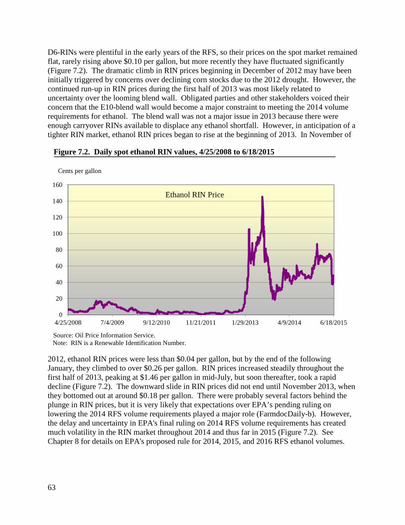
63

D6-RINs were plentiful in the early years of the RFS, so their prices on the spot market remained flat, rarely rising above $0.10 per gallon, but more recently they have fluctuated significantly (Figure 7.2). The dramatic climb in RIN prices beginning in December of 2012 may have been initially triggered by concerns over declining corn stocks due to the 2012 drought. However, the continued run-up in RIN prices during the first half of 2013 was most likely related to uncertainty over the looming blend wall. Obligated parties and other stakeholders voiced their concern that the E10-blend wall would become a major constraint to meeting the 2014 volume requirements for ethanol. The blend wall was not a major issue in 2013 because there were enough carryover RINs available to displace any ethanol shortfall. However, in anticipation of a tighter RIN market, ethanol RIN prices began to rise at the beginning of 2013. In November of

Figure 7.2. Daily spot ethanol RIN values, 4/25/2008 to 6/18/2015

Source: Oil Price Information Service. Note: RIN is a Renewable Identification Number. 2012, ethanol RIN prices were less than $0.04 per gallon, but by the end of the following January, they climbed to over $0.26 per gallon. RIN prices increased steadily throughout the first half of 2013, peaking at $1.46 per gallon in mid-July, but soon thereafter, took a rapid decline (Figure 7.2). The downward slide in RIN prices did not end until November 2013, when they bottomed out at around $0.18 per gallon. There were probably several factors behind the plunge in RIN prices, but it is very likely that expectations over EPA’s pending ruling on lowering the 2014 RFS volume requirements played a major role (FarmdocDaily-b). However, the delay and uncertainty in EPA's final ruling on 2014 RFS volume requirements has created much volatility in the RIN market throughout 2014 and thus far in 2015 (Figure 7.2). See Chapter 8 for details on EPA's proposed rule for 2014, 2015, and 2016 RFS ethanol volumes.

0

20

40

60

80

100

120

140

160

4/25/2008 7/4/2009 9/12/2010 11/21/2011 1/29/2013 4/9/2014 6/18/2015

Cents per gallon

Ethanol RIN Price

64

Most obligated parties, which are primarily oil companies, do not produce ethanol themselves, so they usually obtain RINs by purchasing ethanol. When the ethanol is blended with gasoline, the RINs can be detached and used for compliance purposes, held for future use, or sold. Traders have developed markets for obligated parties and others to buy and sell RINs. As shown in Figure 7.2, RIN prices have become very volatile, for reasons discussed above. When RIN prices skyrocketed in the summer of 2013, many obligated parties, including petroleum companies, argued that the RFS mandates should be eliminated or at least reduced. Others claimed that the 2014 ethanol mandate could be met with 13 billion gallons of E10, along with increased consumption of higher ethanol blends, and carryover RINs from 2013 (Babcock and Pouliot). Although, EPA is in the process of adjusting the 2014 requirement downward, it is likely that the original corn-ethanol mandate of 14.4 billion gallons could have been met. Higher RIN prices can be a signal that more renewable fuel is needed in the system to meet the RFS. If D6-RIN prices are high enough, they can provide an incentive for marketers to sell higher blends of ethanol, if they are able to collect the RIN value. Station owners are not generally obligated parties, so they can sell any RINs they obtain to increase their revenue. Theoretically, the RIN market could stimulate demand and increase investment in the equipment needed to sell large quantities of higher ethanol blends. Maintaining the RFS volume requirements could eventually cause a RIN shortage, along with higher RIN prices, because the blend wall would limit E10 production below the mandates. RIN prices could rise to a point where higher blend markets could become an attractive option for retailers to sell more ethanol and obtain high priced RINs, which can be sold to obligated parties. However, higher blends, such as E15 and E85, have to be priced competitively with E10 (on a gasoline-equivalent basis) to entice consumers to purchase these fuels. Retailers may be willing to discount E15 and E85 prices, since they could be offset by high RIN values.

65

Chapter 8: Policy Challenges and Future Direction of Biofuels James A. Duffield Harry Baumes

Since the implementation of the RFS2 beginning in 2010, the annual requirement for conventional ethanol (mostly corn-ethanol) has been satisfied with little difficulty. There was some concern over corn use for ethanol when a major drought during the 2012 growing season caused a sharp reduction in average corn yields, which fell to 123.4 bushels per acre, the lowest since 1995. U.S. 2012 corn production fell to 10.78 billion bushels, down sharply from early-season projections of 14.8 billion bushels (USDA, Economic Research Service, 2013). Lower corn production led to decreasing stocks and higher prices. The rise in corn prices triggered concerns over higher feed and food prices, prompting Governors of several States to request that the RFS mandates be waived, arguing that the corn required for biofuel production would lead to further supply shortages. However, the U.S. Environmental Protection Agency (EPA) denied the requests after examining the effects a waiver would have on ethanol use, corn prices, and food prices. EPA’s analysis showed that it was highly unlikely that waiving the RFS2 volume requirements would have a significant impact on ethanol production or use in the relevant time frame that a waiver could apply (the 2012/13 corn marketing year, beginning September 1) and therefore little or no impact on corn, food, or fuel prices (EPA, 2012). The drought did cause total U.S. ethanol production to fall in 2012, but the decrease was less than 5 percent. In spite of higher corn prices, the 2012 conventional biofuel requirement of 13.2 billion gallons was satisfied, mostly with ethanol made from U.S. corn. A decrease in ethanol exports was helpful in meeting domestic demand, and a small amount was covered with carryover RINs. The effects of the drought were only temporary, as yields rebounded in 2013 and corn production rose to 13.9 billion bushels. The 2014 corn crop was even larger, setting records for both yields and production at 173.4 bushels per harvested acre and 14.4 billion total bushels (USDA, WASDE, 2015). On the other hand, two major long-term problems are going to make it increasingly difficult to meet future RFS2 total volume requirements. First, the lack of commercially available cellulosic biofuel has made it impossible to meet the cellulosic biofuel requirements originally set by EISA in 2007. The second major issue hampering the implementation of the RFS2 is the E10-blend wall.

Difficulties in Fully Implementing the RFS2

Each year, EPA must determine the projected volume of cellulosic biofuel production for the following year. If the projected volume is less than the applicable volume, EPA must lower the applicable volume accordingly. Consequently, EPA had to lower the cellulosic biofuel requirements for 2010 and 2011, which were originally set at 1 million gallons and 250 million gallons, respectively. Despite EPA’s projections that the industry was positioned to produce about 6 million gallons in each of those years, no RIN-generating biofuels from cellulosic feedstocks were produced. In 2010, the majority of the cellulosic biofuel shortfall was met through the use of RINs generated under the initial RFS regulations, and since there were excess

66

cellulosic RINs, many of these RINs were carried over into the 2011 compliance year. The remaining cellulosic biofuel requirements in 2011 were met by cellulosic biofuel waiver credits that had to be purchased by obligated parties to meet their requirements (Federal Register, 2013b). In 2012, the first cellulosic RINs were generated at two small pilot facilities; however, by this time, it was clear that the biofuel industry was far from capable of producing the 500 million gallons required for that year. The EPA did lower the cellulosic biofuel requirement to the projection of 11.45 million gallons in a final rulemaking on January 2012. However, cellulosic biofuel production once again fell short of the projections in 2012. The 2012 cellulosic standard was challenged in court and, based on the decision in that case, the 2012 cellulosic biofuel volume requirements were vacated (Federal Register, 2013b). The 2013 cellulosic biofuel requirement of 1 billion gallons was reduced to EPA’s projected amount of 6 million gallons (Federal Register, 2013). However, by the end of 2013, it was clear that the 6 million gallons would was not be achieved, and a reassessment by EPA resulted in setting the 2013 cellulosic biofuel requirement to 810,185 gallons (Federal Register, 2014). When EPA reduces the required volume of cellulosic biofuel below the level specified in the statute, it also has the authority to reduce the applicable volumes of advanced biofuels and total renewable fuel by the same or a lesser volume. In years prior to 2014, EPA did not adjust the advanced or total volumes, arguing that shortfall in cellulosic production could reasonably be filled by other advance biofuels, such as biodiesel and imported sugar-based ethanol (Federal Register, 2013b). However, going forward, it will be more and more difficult for other advanced biofuels to make up for the shortfall, as the applicable volumes of cellulosic biofuel become increasingly demanding over time (Figure 8.1). As discussed Chapters 6 and 7, due to the E10-blend wall, the amount of ethanol that can be absorbed into the domestic gasoline pool is currently limited to about 13 billion gallons—well below the 2015 conventional biofuels requirement, which is capped at 15 billion gallons. To exacerbate the problem, the E10-blend wall may become more constraining over time, since gasoline consumption began a declining trend in 2008, due to more efficient motor vehicles, higher prices, weak economic and job growth over the past several years, and fewer miles driven (Figure 8.2). In addition, motor vehicles will continue to become more fuel efficient, as increasingly aggressive corporate average fuel economy (CAFE) standards are implemented. Passenger cars and light trucks are expected to have, on average, a combined fleet-wide fuel economy of about 40 miles per gallon (MPG) in 2021, compared to about 30 MPG in 2013 (National Highway Traffic Safety Administration).

67

Figure 8.1. Renewable fuel standard required volumes, 2008-2022

Figure 8.2. U.S. finished motor gasoline consumption, actual and projected, 1990-2040, billion gallons

Source: U.S. Energy Information Administration, Annual Energy Outlook 2015.

0

5

10

15

20

25

30

35

40

2008 2009 2010 2011 2012 2013 2014 2015 2016 2017 2018 2019 2020 2021 2022

Conventional biofuel Biomass-based diesel

Non-cellulosic advanced biofuel Cellulosic biofuel

60

70

80

90

100

110

120

130

140

150

1990 1995 2000 2005 2010 2015 2020 2025 2030 2035 2040

Billion gallons

Total Advanced

Biofuel

Projections

Billion gallons

68

Proposed Reductions in RFS2 Volume Requirements

In response to concerns from obligated parties and others, EPA announced that it would consider lowering the RFS volume requirements in a future rulemaking. The announcement first came in August 2013, when EPA acknowledged the difficulty of achieving the 2014 RFS, taking into account the available supply of cellulosic biofuel, the availability of advanced biofuel, and the E10-blend wall. The statute set the total renewable fuel volume at 18.15 billion gallons, of which 14.4 billion gallons would be conventional biofuel comprised primarily of corn ethanol and 3.75 billion gal would be advanced biofuel. However, the maximum volume of ethanol that could be consumed, assuming an E10-blend wall, in 2014 was about 13 billion gallons. EPA does not currently foresee a significant amount of ethanol sold in blends greater than E10, and/or see a market that would produce sufficient volumes of non-ethanol biofuels (e.g., biodiesel) to make up for the ethanol shortfall (Federal Register, 2013b). Therefore, a Proposed Rule for the 2014 standards that was released in November 2013 reduced both the total renewable fuel requirement and the advanced biofuel requirement, which were originally set at 18.5 billion gallons and 3.75 billion gallons, respectively. The 2014 adjusted total RFS was set at 15.21 billion gallons, a reduction of 2.94 billion gallons. This amount was based on EPA’s assumptions about the amount of E10 that could be blended into 2014 expected gasoline consumption; the amount of E85 that was expected to be consumed in 2014; and the amount of non-ethanol biofuel (primarily biodiesel) that would be available. The total reduction included 1.55 billion gallons of advanced biofuel, lowering the total advanced RFS from 3.75 billion gallons to 2.2 billion gallons. This resulted in about 13 billion gallons of conventional ethanol to meet the total RFS, a drop of 1.4 billion gallons. Cellulosic biofuel, which is included in the total advanced standard, was set at 17 million gallons. The original statue required 1.75 billion gallons of cellulosic biofuel in 2014. Comments on EPA’s proposed rule were due on January 28, 2014, and a public hearing was held near Washington, DC, on December 5, 2013. Much of the testimony made by ethanol supporters focused on EPA’s assumptions related to the blend wall, arguing that EPA may have underestimated the marketability of higher ethanol blends, so the conventional biofuel standard should be larger. Based on EPA’s analysis, for 2014 they estimated a range of 100-300 million gallons of E85 consumption and zero E15 consumption. EPA used the mean value for E85 consumption, which was about 180 million gallons, or about 133 gallons of pure ethanol. EPA recognizes that E85 consumption could be greater than the mean, especially if E85 prices were discounted relative to E10. While historically, E85 prices have been greater than E10 prices on an energy equivalent basis, there does appear to be a trend emerging in some Midwestern States, where an increasing number of retailers are offering E85 at a discount to E10. If this trend were to continue and become more widespread, E85 consumption could increase. Ethanol supporters argue that a reduction in the RFS would only dampen this trend, because obligated parties will be able to meet their 2014 required volumes without investing in the E85 market. Comments made by opponents of the RFS, including oil refineries and other obligated parties, argued that the EPA’s 2014 proposed volumes were too high. They requested that the 2014 conventional ethanol requirements be set at or below 9.7 percent of 2014 gasoline consumption, which would result in about 12.9 billion gallons of ethanol use. This would help avoid the blend wall and eliminate the necessity of using higher blends to meet the RFS conventional ethanol

69

requirement, set originally at 14.4 billion gallons. In contrast to EPA findings, oil industry groups claim that using ethanol blends greater than E10 is incompatible with conventional engines and current infrastructure (McCormick et al.). In addition, they argue that the RFS biofuel mandates are not necessary, since the Nation’s energy security goals are already being met by the current energy boom in shale development. In their view, the expected increase in domestic oil and natural gas supplies will more than satisfy U.S. future energy needs; and they vow to continue their fight in repealing the RFS. In December 2014, EPA announced that they would not be finalizing the 2014 volume requirements until 2015 (EPA, 2014). This delay prompted a lawsuit against EPA by the American Petroleum Institute and the American Fuel and Petrochemical Manufacturers. In litigation brought against EPA, the Agency announced on April 10, 2015, a proposed consent decree that would establish schedules for issuing the 2014 and 2015 renewable fuel standards (EPA, 2015). On June 1, 2015, EPA proposed Renewable Fuel Standards for 2014 through 2016, and the Biomass-Based Diesel Volume for 2017. The final rule is expected to be finalized by November 30, 2015. EPA determined that the November 2013 proposal required modification and therefore must be withdrawn, since projecting volume growth into the then future had to be adjusted given the significant amount of time that had passed (Federal Register, 2015). With the new timeframe, EPA also determined that the November, 2013 proposal likely overestimated the volumes reductions needed to adjust the RFS, hence the new proposed volumes were adjusted upward. Since the proposal occurred after 2014, EPA proposed to use actual 2014 renewable fuel volumes for the 2014 RFS. Actual renewable fuel use was based on the total number of Renewable Identification Numbers (RINs) collected by EPA, minus the RINs associated with renewable fuel exports and other noncompliance RINs (Federal Register, 2015). Based on this approach, EPA set the 2014 RFS for ethanol at 13.25 billion gallons—about 250 million gallons higher than the original proposed 2014 volume requirement. The 2015 and 2016 proposed volumes were set below the statute levels, but not as much as in the original proposal. A market evaluation by EPA concluded that the E10 blend wall would restrict conventional ethanol consumption below the 15 billion gallon RFS set for 2015. However, EPA assumed there would be some ethanol growth in 2015 and further growth in 2016. Therefore, the 2015 conventional ethanol volume was set at 13.4 billion gallons or 150 million gallons above the 2014 volume. The 2015 conventional ethanol volume is increased another 600 million gallons to14 billion gallons—1 billion gallons below the original 15 billion gallons set by the statute. The 2014 cellulosic biofuel RFS, which includes cellulosic ethanol, was set at 33 million gallons, well short of the 1.75 billion gallons set by the statute, but significantly above the 17 million gallons set by the original 2013 proposal. The 2014 cellulosic biofuel volume requirement was based on actual 2014 volumes using RIN data, as explained above. EPA believes that the cellulosic biofuel industry has made significant progress over the past several years, and expects cellulosic biofuel production to grow to 106 million gallons in 2015 and 206 million gallons in 2016 (Federal Register, 2015).

70

If the proposal is finalized by November 30, 2015, as planned, EPA will be up-to-date with issuing RFS annual rules. However, blend wall constraints on the RFS are expected to persist beyond 2016, so each year EPA will assess the current situation, including the growing markets for E15 and E85, to help determine the amount of ethanol that is expected to be consumed and adjust the RFS accordingly. Future Direction of Biofuels Congress recognized that the 36-billion-gallon RFS2 could not be met with corn ethanol alone, thus it included requirements for cellulosic biofuel, biomass-based diesel, and other advanced biofuels that together reach a total of 21 billion gallons by 2022. Allowing the ethanol tax credit and import duty (see chapter 1 for more details) to expire was a signal from policymakers that the corn ethanol industry had reached some degree of maturity and that the RFS2 would be sufficient for sustaining future production. Since the 1970s, the ethanol industry has grown from a few small firms to about 200 plants operating in 29 States, with an annual operating capacity of 14.6 billion gallons (Renewable Fuels Association, 2015). It provides a major market for U.S. corn production, benefits many farmers, and generates a significant number of jobs in rural areas, where job creation is difficult (Pender et al.). Ethanol has become fully integrated into the U.S. fuel infrastructure to the extent that most gasoline sold today contains about 10 percent ethanol. Although EPA has approved the use of E15 in 2001 and newer vehicles, it is not currently available at most retail outlets. However, a market for E15 is beginning to grow, as it is sold in over 100 stations across 16 States (Renewable Fuels Association, 2015). The E15 market could grow significantly in the near future, since many stations already use equipment that is E15 compatible. Overtime, as other station owners upgrade their equipment, they can purchase E15 compatible equipment at an additional minimal cost (Moriarty and Yanowitz). There are more than 17 million FFVs on the road today that can use higher blend levels, up to 83 percent, but most filling stations do not offer higher blends and FFVs have had little effect on ethanol demand (Alternative Fuels Data Center-a). Future growth in U.S. ethanol consumption will depend on new markets and infrastructure for higher blends. Also, if U.S. ethanol capacity remains above domestic market needs, the industry will look to increase sales to foreign markets. U.S. ethanol exports have increased significantly since 2010, and the United States became the world's largest exporter of ethanol in 2011, and again in 2014, exporting 836 million gallons (USDA, Foreign Agricultural Service). It is unclear at this time how quickly U.S. consumers will be able or willing to increase consumption of E15 and E85. The U.S. Energy Information Administration (EIA) projections show the ethanol used in E85 increasing significantly between 2025 and 2040, with an annual average growth rate of almost 10 percent from 2013 to 2040 (EIA, 2015). The conventional biofuels mandate reaches a limit of 15 billion gallons per year starting in 2015, which is only about 2 billion gallons over the current E10-blend wall. Thus, it is conceivable that potential E15 and E85 growth would eventually satisfy this volume requirement. In the case of cellulosic ethanol, the blend wall does not appear to be an immediate problem, since the commercialization of these biofuels has been advancing slowly, and it is unlikely they will be entering the marketplace in significant volumes soon.

71

Even though EPA plans to adjust the RFS mandates to account for the blend wall and realign the total advanced biofuel mandates with current projected trends, the overall goals of the program to support growth in renewable fuels are still in place. However, in order to meet these long-term goals, Federal and State support designed to incentivize investments in E85 infrastructure and cellulosic biofuels will have to continue. Investment in cellulosic biofuels that use technologies to convert hydrocarbons into “drop-in biofuels” would be particularly helpful, since these fuels can be integrated into the current petroleum fuel infrastructure seamlessly. With investment from Government Agencies and private companies, drop-in biofuels, such as renewable gasoline and butanol, are currently under development (U.S. Department of Energy, 2015). Perhaps in the near future, cellulosic feedstocks will be converted into significant volumes of renewable gasoline and other drop-in biofuels. Renewable gasoline would not be subject to the blend wall and could help meet the total advanced biofuel requirements of the RFS. While continued Government support is needed to help stimulate investment in advanced biofuel production, it has become more difficult to fund biofuel programs due to the current efforts by Congress to cut Government spending and reduce the deficit. It is also being argued by some that programs like the RFS are no longer needed, because new sources of fossil energy in North America negate the necessity of investing public dollars in renewable energy development. With recent advances in drilling technologies, large new reserves of oil and gas have become available in Canada and the United States. Oil prices have already felt the effect of these new sources of energy supplies with prices starting a steady decline in June, 2014—falling from about $100 per barrel to about $50 per barrel by the end of 2014, where they leveled off, as of May, 2015. More optimistic energy forecasts could make public investment in biofuels a lower priority in future energy policies. However, it seems unlikely that policymakers would abandon their efforts to diversify the U.S. fuel supply. For over 20 years, U.S. energy policy has viewed fuel diversification as part of a long-run strategy to increase energy security and reduce harmful air emissions from motor vehicles. While the recent energy boom is helping the Nation become more energy independent, fuel diversification is likely to remain an important component of our long-term clean energy strategy. Although new energy legislation is not expected anytime soon, there have been several proposals to modify the RFS. When Congress does begin to discuss new energy legislation, there will likely be much debate over the future direction of the RFS and how scarce dollars should be spent to support continued growth of the biofuels industry. There undoubtedly will be vigorous debate over finding a solution to the blend wall—should the Government invest in an E85 infrastructure to accommodate more ethanol, or should the focus be more on research to advance the technology of drop-in biofuels? It is difficult to predict future U.S. energy legislation, but as in the past, policy is expected to play a critical role in shaping the biofuels industry.

72

References Alternative Fuels Data Center-a. U.S. Department of Energy, Energy Efficiency and Renewable Energy. Available at: http://www.afdc.energy.gov/vehicles/flexible_fuel.html. Accessed on April 20, 2015. Alternative Fuels Data Center-b. U.S. Department of Energy, Energy Efficiency and Renewable Energy. Clean Cities Alternative Fuels Price Reports. Available at: http://www.afdc.energy.gov/fuels/prices.html. Alternative Fuels Data Center-c. U.S. Department of Energy, Energy Efficiency and Renewable Energy. Available at: http://www.afdc.energy.gov/afdc/laws/search. Babcock, B. and S. Pouloit. Feasibility and Cost of Increasing US Ethanol Consumption Beyond E10. CARD Policy Briefs, Iowa State University, 14-PB 17, January 2014. Bevill, K. Minnesota extends E20 mandate to start in 2015. Ethanol Producer Magazine, May 8, 2012. Available at http://ethanolproducer.com/articles/8767/minnesota-extends-e20-mandate-to-start-in-2015. Accessed on March 28, 2014. Brechbill S.C. and Tyner W. E. State Biofuels Policy, SunGrant BioWeb. Available at: http://bioweb.sungrant.org/General/Policy/State+Biofuels+Policy/Default.htm (last updated February 4, 2008). California Air Resources Board (CARB), California Environmental Protection Agency. Low Carbon Fuel Program, LCFS Lookup Tables as of 2012. Available at: http://www.arb.ca.gov/fuels/lcfs/lcfs.htm. Accessed on May 8, 2014. Chandler, K., Whalen M. and Westhoven J. Final Results from the State of Ohio Ethanol-fueled Light-duty Fleet Deployment Project. National Renewable Energy Laboratory, U.S. Department of Energy, NREL/CP-54-17083, Golden Colorado, August 1998. Denicoff, Marina, J. Hill, N. Marathon, B. McGregor, M. Prater, and A. Taylor. Ethanol Transportation Backgrounder: Expansion of US Corn-based Ethanol from the Agricultural Transportation Perspective, U.S. Department of Agriculture, Agricultural Marketing Service, September 2007. http://dx.doi.org/10.9752/TS029.09-2007. Denicoff, M., M. Prater, and P. Bahizi. Corn Transportation Profile, AMS Transportation and Marketing Programs, U.S. Department of Agriculture, Agricultural Marketing Service. August 2014. Available at: http://www.ams.usda.gov/AMSv1.0/getfile?dDocName=STELPRDC5108805 Duffield, J.A., and K. Collins. 2006. Evolution of Renewable Energy Policy, Choices, 1st Quarter, 21(1).

73

Duffield, J. A., Xiarchos, I., and S. Halbrook. 2008. Ethanol Policy: Past, Present, and Future, University of South Dakota, South Dakota Law Journal, Vol. 53(3), pp. 425-53. Ethanol Producer Magazine. January 4, 2010. Incentives: It's All About Location, Location, Location. Available at: http://www.ethanolproducer.com/articles/6248/incentives-it's-all-about-location-location-location/. FarmdocDaily-a. December 27, 2013. RIN Update: 2014 Carry In and EPA’s Proposed Rule. Department of Agriculture and Consumer Economics, University of Illinois, Urbana-Champaign. Available at: http://farmdocdaily.illinois.edu/2013/12/rin-update-2014-carry-in-epa-rulemaking.html. FarmdocDaily-b. October 10, 2013. What’s Behind the Plunge in RINs Prices? Department of Agriculture and Consumer Economics, University of Illinois, Urbana-Champaign. Available at: http://farmdocdaily.illinois.edu/2013/10/whats-behind-the-plunge-in-rin.html . Federal Highway Administration, Department of Transportation. Highway Statistics 2012. Table VM-1. Office of Highway Policy Information, January 2014. Available at: http://www.fhwa.dot.gov/policyinformation/statistics/2012/vm1.cfm. Federal Register. 2007. Regulation of Fuels and Fuel Additives: Renewable Fuel Standard Program: Final Rule. U.S. Environmental Protection Agency, Vol. 72, No. 83, May 1, 2007, Part II. Available at: http://www.gpo.gov/fdsys/pkg/FR-2007-05-01/html/E7-7140.htm. Federal Register. 2010. Regulation of Fuels and Fuel Additives: Changes to Renewable Fuel Standard Program; Final Rule. U.S. Environmental Protection Agency, Vol. 75, No. 58, March 26, 2010, Part II. Available at: http://www.gpo.gov/fdsys/pkg/FR-2010-03-26/pdf/2010-3851.pdf. Federal Register. 2010a. Light-Duty Vehicle Greenhouse Gas Emission Standards and Corporate Average Fuel Economy Standards; Final, Rule, U.S. Environmental Protection Agency and U.S. Department of Transportation, Vol. 75. No. 88, May 7, 2010. Available at: http://www.gpo.gov/fdsys/pkg/FR-2010-05-07/pdf/2010-8159.pdf. Federal Register. 2013a. Regulation of Fuels and Fuel Additives: 2013 Renewable Fuel Standards, Final Rule. U.S. Environmental Protection Agency, Vol.78, No. 158, August 15, 2013, Part II. Available at: http://www.gpo.gov/fdsys/pkg/FR-2013-08-15/pdf/2013-19557.pdf. Federal Register. 2013b. 2014. Standards for the Renewable Fuel Standard Program: Proposed Rule, U.S. Environmental Protection Agency, Vol.78. No. 230, November 29, 2013. Available at: http://www.gpo.gov/fdsys/pkg/FR-2013-11-29/pdf/2013-28155.pdf. Federal Register. 2014. Regulation of Fuels and Fuel Additives: 2013 Cellulosic Biofuel Standard, Final Rule. U.S. Environmental Protection Agency, Vol. 79, No. 85, May 2, 2014. Available at: http://www.gpo.gov/fdsys/pkg/FR-2014-05-02/pdf/2014-10135.pdf.

74

Federal Register. 2015. Renewable Fuel Standard Program: Standards for 2014, 2015, and 2016 and Biomass-Based Diesel Volume for 2017. U.S. Environmental Protection Agency, Vol. 80, No. 111, June 10, 2015. Available at: http://www.epa.gov/otaq/fuels/renewablefuels/regulations.htm. Ford Motor Company Staff, “Ethanol Optimized Engine,” USDA Biofuel Seminar Series, March 29, 2011. Gallagher, P. “Development of the Corn-Ethanol Industry in the United States: Roles for Evolving Markets, Technology, and Policy,” in Regional Economic Development (Federal Reserve Bank of St. Louis), p. 26, April 2009. Gallagher, P., H. Shapouri, and H. Brubaker. 2007. “Scale, Organization and Profitability of Ethanol Processing,” Canadian Journal of Agricultural Economics, 55(2007):63-81. Gallagher, P. and H. Shapouri. 2009. “Improving Sustainability of the Corn-Ethanol Industry,” in Biofuels, W. Soetaert and E. Vandamme, eds, John Wiley, West Sussex (UK), February 2009. Gallagher, P., H. Shapouri, J. Price, G. Schamel, and H. Brubaker. 2003. “Some Long-Run Effects of Growing Fuel Markets, MTBE Bans and Renewable Averaging Policies on Additives Markets and the Ethanol Industry,” Journal of Policy Modeling, 25 (September 2003):585-608. Gallagher, P, D. Otto, and M. Dikeman. 2000. “Effects of an Oxygen Requirement for Fuel in Midwest Ethanol Markets and Local Economies,” Review of Agricultural Economics, 22 (November 2000):292-311. Gantz, Rachel. “South Dakota to Use E15 Blends in State Fleet for Six-Month Trial,” OPIS, Biofuels Update, March 7, 2014. Copyright, Oil Price Information Service. Green Car Congress. Energy, Technologies, Issues and Policies for Sustainability Mobility. Available at: http://www.greencarcongress.com/. Iowa Renewable Fuels Association. Big Oil Using Distribution Monopoly to Keep Low-Cost, Homegrown E15 Out of Iowa. Iowa Renewable Fuels Association Press Release, June 2, 2013, Available at http://www.iowarfa.org/LinnCoopE15Event.php. Accessed on March 28, 2014. Jennings, M.J. 2007. Note: Bioenergy: Fueling the Future? Drake Journal of Agricultural Law (12), pp 205,-213 Jessen, H. New State Law Protects Retailers' Right to Offer Ethanol Blends, May 24, 2013, Ethanol Producer Magazine. Available at http://www.ethanolproducer.com/articles/9893/new-state-law-protects-retailers-right-to-offer-ethanol-blends. Accessed on March 28, 2014. Liu, Changzheng, and David L. Greene. Light Duty Vehicle Markets & E85: Theory, Econometrics & Modeling,” EIA Biofuels Workshop, Washington, D.C., March 20, 2013.

75

McCarthy, J. E. and M. Tiemann. MTBE in Gasoline: Clean Air and Drinking Water Issues, Congressional Research Service Reports Paper 26. Congressional Research Service. Available at: http://digitalcommons.unl.edu/cgi/viewcontent.cgi?article=1025&context=crsdocs. McCormick, R., J. Yanowitz, J., Ratcliff, M., and B. Zigler. Review and Evaluation of Studies on the Use of E15 in Light-Weight Vehicles. National Renewable Energy Laboratory, Golden CO. Prepared for the Renewable Fuels Association, October 2013. Moriarty, Kristi. “E85 Deployment,” EIA Biofuels Workshop, Washington, D.C., March 20, 2013. Available at: http://www.eia.gov/biofuels/workshop/presentations/2013/ Moriarty, K. and J. Yanowitz. 2015. E15 and Infrastructure. National Renewable Energy Laboratory. June, 2015. Available at: http://www.byoethanol.com/images/stories/PDFs/NRELE15andInfrastructure2.pdf. National Highway Traffic Safety Administration. Corporate Average Fuel Economy (CAFE). DOT and EPA Establish CAFE and GHG Emissions Standards for Model Years 2017 and Beyond. Available at: http://www.nhtsa.gov/fuel-economy. Assessed April 21, 2015. National Agricultural Law Center. An Agricultural Law Research Project: Biofuels Statutory Citations, United States Federal Laws, Assembled by Shannon Mirus, University of Arkansas. Available at: http://nationalaglawcenter.org/wpcontent/uploads/assets/articles/mirus_federalbiofuel.pdf Accessed July 27, 2015. Pender, J. Marre, A. and R. Reader. 2012. Rural Wealth Creation: Concepts, Strategies, and Measures. U.S. Department of Agriculture, Economic Research Service, Economic Research Report No. 131, March 2012. Available at: http://www.ers.usda.gov/media/365520/err131_1_.pdf. Reynolds, R. Changes in Gasoline IV: The Auto Technician’s Guide to Spark Ignition Engine Fuel Quality, Downstream Alternatives, Renewable Fuels Foundation, South Bend, IN, June 2009. Available at: http://www.ethanolrfa.org/page/-/rfa-association-site/ChangesinGasolineManualIV-UpdatedLogo.pdf?nocdn=1. Shapouri, H., Graboski, M. and P. Gallagher. 2000. USDA’s 1998 Ethanol Cost-of-Production Survey, U.S. Department of Agriculture, Office of Energy Policy and New Uses, Agricultural Economic Report No. 808. 2000. Shapouri, H. and P. Gallagher. 2005. USDA’s 2002 Ethanol Cost-of-Production Survey, U.S. Department of Agriculture, Office of Energy Policy and New Uses, Agricultural Economic Report No. 841, July 2005.

76

Shapouri, H., P. Gallagher, W. Nefstead, R. Schwartz, S. Noe, and R. Conway. 2010. 2008 Energy Balance for the Corn-Ethanol Industry, AER No. 846, Office of Energy Policy and New Uses, U.S. Department of Agriculture, March 2010. Shockey, R.E. and T.R. Aulich, “Optimal Ethanol Blend-Level Investigation,” Energy and Environment Research Center (University of North Dakota) and Minnesota Center for Automotive Research (Minnesota State University, Report 2007-EERC-11-02, Grand Forks North Dakota, November 2007. Thompson, W., Meyer, S., and P. Westhoff. 2009. Renewable Identification Numbers are the Tracking Instrument and Bellwether of U.S. Biofuel Mandates. EuroChoices, Vol. 8(3), June 2009. Available at: http://onlinelibrary.wiley.com/doi/10.1111/j.1746-692X.2009.00133.x/pdf. Tyner, W. National and Global Market Implications of the 2012 U.S. Drought. Global Agricultural Development Initiative, Issue Briefs Series, The Chicago Council on Global Affairs. February 2013. U.S. Department of Agriculture (USDA). 2010. Advancing Renewable Energy (pamphlet), October 2010, revised May 2011. Available at: http://www.usda.gov/energy/maps/resources/brochure/$file/renewable_energy_brochure.pdf. U.S. Department of Agriculture, Economic Research Service. 2013. U.S. Drought 2012: Farm and Food Impacts. Available at: http://www.ers.usda.gov/topics/in-the-news/us-drought-2012-farm-and-food-impacts.aspx. Accessed on August 22, 2013. U.S. Department of Agriculture, Economic Research Service. 2014. Agricultural Act of 2014: Highlights and Implications. Available at: http://www.ers.usda.gov/agricultural-act-of-2014-highlights-and-implications/energy.aspx. U.S. Department of Agriculture, Agricultural Marketing Service. Transportation of U.S. Grains: A Modal Share Analysis 1978-2011, May 2013. Available at: http://www.ams.usda.gov/AMSv1.0/AgTransportation. U.S. Department of Agriculture, Agricultural Marketing Service. Transportation of U.S. Grains: A Modal Share Analysis 1978-2010, March 2010. Available at: http://www.ams.usda.gov/AMSv1.0/AgTransportation. U.S. Department of Agriculture, Farm Service Agency. Biomass Crop Assistance Program. Available at http://www.fsa.usda.gov/programs-and-services/energy-programs/BCAP/index. Assessed June 12, 2015. U.S. Department of Agriculture, Foreign Agricultural Service. U.S. Ethanol Exports Rebound in 2014. International Agricultural Trade Reports, May 1, 2015. Available at: http://www.fas.usda.gov/data/us-ethanol-exports-rebound-2014.

77

U.S. Department of Agriculture, National Agricultural Statistics Service. Charts and Maps / Field Crops. Available at: http://www.nass.usda.gov/Charts_and_Maps/Field_Crops/cornyld.asp. Accessed on June 26, 2015. U.S. Department of Energy (DOE). 2010. Report to Congress, Dedicated Ethanol Pipeline Feasibility Study, Energy Independence and Security Act of 2007, Section 243, March 2010. Available at: https://www1.eere.energy.gov/bioenergy/pdfs/report_to_congress_ethanol_pipeline.pdf. U.S. Department of Energy (DOE). 2012. Biomass Multi-Year Program Plan, April 2012. Energy Efficiency & Renewable Energy. Available at: http://www1.eere.energy.gov/bioenergy/pdfs/mypp_april_2012.pdf. U.S. Department of Energy (DOE). 2015. Office of Energy Efficiency and Renewable Energy. Research, Development, Demonstration, and Deployment. Available at: http://www.energy.gov/eere/bioenergy/research-development-demonstration-and-deployment. Assessed June 12, 2015. Unzelman, G. H. 1992. Implementing the Clean Air Act: Fuel Reformulation and Regulation in the 1990’s: An Analysis of Reformulated Gasoline and Oxygenated Fuels, 1992-2000. Information Resources, Inc. U.S. Energy Information Administration (EIA). 2009. Annual Energy Outlook with Projections to 2030. DOE/EIA-0383(2009), March 2009. Available at: http://www.eia.gov/oiaf/aeo/pdf/0383(2009).pdf. U.S. Energy Information Administration (EIA). 2012. Petroleum Administration for Defense Districts. Available at: http://www.eia.gov/todayinenergy/detail.cfm?id=4890&src=email. Accessed on April, 8, 2015. U.S. Energy Information Administration (EIA). 2013. Petroleum Marketing Monthly, July 2013, Office of Petroleum and Biofuels Statistics, U.S. Department of Energy, P. 40. Available at: http://www.eia.gov/petroleum/marketing/monthly/pdf/pmmall.pdf. U.S. Energy Information Administration (EIA). Petroleum and Other Liquids. U.S. Product Supplied of Finished Motor Gasoline. Available at: http://www.eia.gov/dnav/pet/hist/LeafHandler.ashx?n=PET&s=MGFUPUS1&f=A. Assessed on August 10, 2015. U.S. Energy Information Administration (EIA). 2015. Annual Energy Outlook 2015 with Projections to 2040, April, 2015. Available at: http://www.eia.gov/forecasts/aeo/pdf/0383(2015).pdf

78

U.S. Environmental Protection Agency (EPA). 2010a. Regulatory Announcement: EPA Finalizes Regulations for the National Renewable Fuel Standard Program for 2010 and beyond. Office of Transportation and Air Quality, EPA-420-F-10-007. Available at: http://www.epa.gov/otaq/renewablefuels/420f10007.pdf. U.S. Environmental Protection Agency (EPA). New Fuel Pathways website. Available at: U.S. Environmental Protection Agency (EPA). Assessed on May 28, 2015. U.S. Environmental Protection Agency. 1999. Achieving Clean Air and Clean Water: The Report of the Blue Ribbon Panel on Oxygenates in Gasoline. Available at: http://www.epa.gov/oms/consumer/fuels/oxypanel/r99021.pdf. Accessed on March 28, 2014. U.S. Environmental Protection Agency (EPA). 2010b. Renewable Fuels Standard Program (RFS2) Regulatory Impact Analysis. Assessment and Standards Division, Office of Transportation and Air Quality, EPA-420-R-10-006, February 2010. Available at: http://www.epa.gov/otaq/renewablefuels/420r10006.pdf. U.S. Environmental Protection Agency (EPA). 2012. Regulatory Announcement: EPA Decision to Deny Requests for Waiver of the Renewable Fuel Standard. Office of Transportation and Air Quality, EPA-420-F-12-075, November 2012. Available at: http://www.epa.gov/otaq/fuels/renewablefuels/documents/420f12075.pdf. U.S. Environmental Protection Agency. 2013. The Official U.S. Government Source for Fuel Economy Information. Available at: http://www.fueleconomy.gov/feg/pdfs/guides/FEG2014.pdf, Accessed September 13, 2013. U.S. Environmental Protection Agency. 2014. Notice of Delay in Issuing 2014 Standards for the Renewable Fuel Standard Program. Available at: http://epa.gov/otaq/fuels/renewablefuels/regulations.htm. U.S. Environmental Protection Agency. 2015. Renewable Fuels Volume Standards Timeline Announced. Available at: http://epa.gov/otaq/fuels/renewablefuels/regulations.htm. Rhodes, Anne. California Plans to Ban MTBE from Gasoline, 97 OIL & GAS J. 39 (Apr. 5, 1999). Renewable Fuels Association. 2015. The New Fuel: E15. Available at: http://www.ethanolrfa.org/pages/E15. Accessed April 17, 2015. Renewable Fuels Association. 2013. 2013 Ethanol Industry Outlook. Battling for the Barrel. Available at: http://www.ethanolrfa.org/pages/annual-industry-outlook Renewable Fuels Association. 2015. 2015 Ethanol Industry Outlook. Going Global. Available at: http://www.ethanolrfa.org/pages/annual-industry-outlook

79

West, B., K. Knoll, W. Clark, R. Graves, J. Orban, S. Przesmitzki, and T. Theiss. Effects of Intermediate Ethanol Blends on Legacy Vehicles and Small NonRoad Engines, Report 1, National Renewable Energy Lab and Oak Ridge National Lab, NREL/TP-540-43543 and ORNL/TM-2008/117, October 2008. Westcott, P., and L. McPhail. 2013. High RIN Prices Signal Constraints to U.S. Ethanol Expansion. Feed Outlook: Special Article, Economic Research Service, USDA, Situation and Outlook, FDS-13d-SA, April 12, 2013. Available at: http://www.ers.usda.gov/media/1158986/fds-13d-sa.pdf. Yacobucci, B. 2011. Biofuels Incentives: A Summary of Federal Programs, CRS Report for Congress, Congressional Research Service: Available at http://fpc.state.gov/documents/organization/168094.pdf. Yea, S. and J. Whitcover. Status Review of California’s Low Carbon Fuel Standard. U.C. Davis, Institute of Transportation Studies, Research Report—UCD-ITS-RR-14-01, January 2014 Issue.

80

Appendix

Appendix Table 1 – Summary of key legislation related to ethanol, 1978-1999 Title of Legislation

Description National Energy Act of 1978

The first major piece of legislation related to ethanol that gave ethanol blends of at least 10 percent a $0.40-per-gallon exemption from the Federal motor fuels tax. Due to changes in excise taxes on motor fuels in 1983, the tax exemption for ethanol increased to $0.50 per gallon.

Energy Security Act of 1980

Offered insured loans to small ethanol plants producing less than 1 million gallons per year. The U.S. Secretaries of Agriculture and Energy were ordered to prepare a plan that would increase ethanol production to at least 10 percent of total gasoline supply by the end of 1990.

Crude Oil Windfall Profit Tax Act (1980)

Extended the motor fuels tax exemption through 1992, and provided blenders the option of receiving the same tax benefits by using an income tax credit instead of the fuel tax exemption.

Omnibus Reconciliation Act of 1980

Established a 2.5-percent ad valorem tariff and an import duty on ethanol of $0.54 per gallon.

Caribbean Basin Initiative (1983)

Shortly after Congress first adopted the motor fuel tax credit, it also enacted a duty on fuel ethanol imports to offset the value of the Federal tax exemption, so foreign ethanol producers could not benefit from the exemption. Duty-free treatment for ethanol was granted to 22 Caribbean Basin countries and territories in January 1984, under the Caribbean Basin Initiative.

Deficit Reduction Act of 1984

The ethanol tax exemption and blenders income tax credit were raised to $0.60 per gallon.

Alternative Motor Fuels Act (1988)

Provides credits to automakers towards meeting their corporate average fuel efficiency (CAFE) standards for manufacturing alternative-fueled vehicles, including E85s.

81

Appendix Table 1 – Summary of Key Legislation Related to Ethanol, 1978-1999, continued Omnibus Budget Reconciliation Act (1990)

Lowered the ethanol tax exemption and blenders income tax credit to $0.54 per gallon. The expiration date for the new tax rates was extended to 2002. The Act also provided a $0.10 per gallon payment to small ethanol producers with a capacity of 30 million gallons or less. Producers could receive the tax credit up to 15 million gallons of production annually.

Clean Air Act Amendments of 1990 (CAAA)

Provisions of the CAAA established the Oxygenated Fuels Program and the Reformulated Gasoline (RFG) Program to control carbon monoxide and ozone problems in certain urban areas around the country that were judged to be in “non-attainment.” Both program fuels required 2 percent oxygen, and ethanol became a popular oxygenate for producers to blend with gasoline to meet the new oxygen requirements mandated by the CAAA. However, the more marketable oxygenate at that time was MTBE.

Energy Policy Act of 1992 (EPACT)

EPACT extended the fuel tax exemption and the blenders’ income tax credit to two additional blend rates containing less than 10 percent ethanol, effective January 1, 1993 (National Agricultural Law Center). The two additional blend rates were for gasoline with at least 7.7 percent ethanol and for gasoline with 5.7 percent ethanol. These additional blends were added to encourage blending of ethanol to make oxygenated gasoline in the Oxygenated Fuels Program, requiring 7.7 percent ethanol, and in the Reformulated Gasoline (RFG) Program, which requires 5.7 percent ethanol. This act also required Federal agencies to purchase a certain percentage of alternative-fuel vehicles, including E85s.

Transportation Equity Act for the 21st Century (1998)

Reduced the ethanol tax exemption and blenders’ income tax credit to $0.53 starting January 2001, reducing it further to $0.52 in January 2003 and to $0.51 in January 2005. Both tax credits were extended to the end of 2007.

California Banned MTBE (1999)

MTBE was banned in California at the earliest possible date, but no later than December 31, 2002. This date was amended, in March 2002, to December 31, 2003. Following California’s lead, at least 24 other States also banned MTBE, allowing ethanol to become the dominate fuel in the oxygenate market.

82

Appendix Figure 1. Ethanol trade flows by PADDs, billion gallons, 2012

Note: PADDs are Petroleum Administration for Defense Districts Source: Energy Information Agency, U.S. Dept. of Energy: http://www.eia.gov/dnav/pet/pet_move_ptb_dc_R20-R10_mbbl_m.htm

Where: Qi = Output from origin i, Dj = Demand for destination j, Sij = Shipments from origin i to destination j, Mj = Imports to destination j, Xi = Exports from destination j.

Q4=0.2 D4=0.4

PADD 4

PADD 5

PADD 3

Q3=0.3 D3=1.9

PADD 2

Q2=12.3 = D2= 3.4

PADD 1

Q2=0.3 D2=4.8

Q5=0.2 D5=2.2

S21=4.3

S24= 0.2

S25=2.0 S23=2.0

M5=0.1 M1=0.4 X2=0.3 X3=0.4